Seediscussions,stats,andauthorprofilesforthispublicationat:https://www.researchgate.net/publication/303939596

InfiniteResolutionTextures

ConferencePaper·June2016

CITATIONS

0

READS

1,086

2authors,including:

AlexanderReshetov

NVIDIA

19PUBLICATIONS410CITATIONS

SEEPROFILE

AllcontentfollowingthispagewasuploadedbyAlexanderReshetovon14June2016.

Theuserhasrequestedenhancementofthedownloadedfile.Allin-textreferencesunderlinedinblueareaddedtotheoriginaldocument

andarelinkedtopublicationsonResearchGate,lettingyouaccessandreadthemimmediately.

High Performance Graphics (2016)Ulf Assarsson and Warren Hunt (Editors)

Infinite Resolution Textures

Alexander Reshetov and David Luebke

NVIDIA

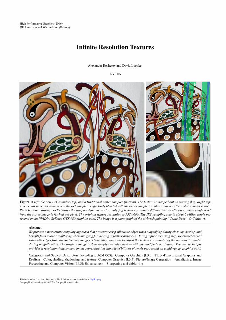
Figure 1: left: the new IRT sampler (top) and a traditional raster sampler (bottom). The texture is mapped onto a waving flag. Right top:

green color indicates areas where the IRT sampler is effectively blended with the raster sampler; in blue areas only the raster sampler is used.

Right bottom: close-up. IRT chooses the sampler dynamically by analyzing texture coordinate differentials. In all cases, only a single texel

from the raster image is fetched per pixel. The original texture resolution is 533×606. The IRT sampling rate is about 6 billion texels per

second on an NVIDIA GeForce GTX 980 graphics card. The image is a photograph of the airbrush painting “Celtic Deer” © CelticArt.

Abstract

We propose a new texture sampling approach that preserves crisp silhouette edges when magnifying during close-up viewing, and

benefits from image pre-filtering when minifying for viewing at farther distances. During a pre-processing step, we extract curved

silhouette edges from the underlying images. These edges are used to adjust the texture coordinates of the requested samples

during magnification. The original image is then sampled — only once! — with the modified coordinates. The new technique

provides a resolution-independent image representation capable of billions of texels per second on a mid-range graphics card.

Categories and Subject Descriptors (according to ACM CCS): Computer Graphics [I.3.3]: Three-Dimensional Graphics andRealism—Color, shading, shadowing, and texture; Computer Graphics [I.3.3]: Picture/Image Generation—Antialiasing; ImageProcessing and Computer Vision [I.4.3]: Enhancement—Sharpening and deblurring

This is the authors’ version of the paper. The definitive version is available at diglib.eg.org.Eurographics Proceedings © 2016 The Eurographics Association.

A. Reshetov & D. Luebke / Infinite Resolution Textures

1. Introduction

Graphics applications such as games combine 3D geometric dataand 2D textures. These assets behave differently under scaling. The3D data represents the shape of the objects in a scene and as suchcan be sampled at any resolution. 2D textures are typically used torepresent material properties and minute geometric details, and havea limited resolution defined by the underlying image. Unlike 3Dmodels, textures can be easily pre-filtered at multiple coarse levelsand stored in a mipmapped format. This is a significant advantage,as it allows integrating over all subsamples in a pixel by issuing asingle texel fetch. Using trilinear mipmapping [Wil83], the level ofdetail can vary smoothly, so when a computer graphics object movesaway from the viewpoint, its texturing will change gradually fromthe fine to the coarse levels. Unfortunately, when we zoom in onsuch an object, the pixels in even the highest-detail texture imagewill eventually become larger than the pixels on the screen. Whenthis happens we will see a familiar blotchy structure of the textureand the image will become over-blurred.

Ironically, this wasn’t always the case. The earliest 2D computergraphics were all based on such geometric primitives as straightand curved line segments, directly rendered on vector displays. Thewide use of discrete raster images came later, supported by the rapiddevelopment of raster displays and hardware texture samplers.

Vector graphics continue to proliferate in areas in which qualityapproximation is not acceptable, such as professional graphics. Thisincludes, in particular, illustration and computer-aided design. Vectorgraphics allow storing data in a resolution-independent format whichcan then be rendered on any device or printed as a hard copy. Mostvector graphics formats (such as PostScript or SVG) can be treatedas programs prescribing the process of rendering an image composedof (potentially overlapping) geometric primitives. For this reason,computing a color at a single position might necessitate executing thewhole program. This is not an issue in professional applications whenthe whole image emerges as a result of executing such a program,but it makes vector graphics a less efficient substitute for textureassets in games, where often only a portion of an image is accessedevery frame and samples are irregularly distributed.

Vector graphics formats, considered as programs, tend to be se-quential in nature. This hindered their hardware optimization, untilthe groundbreaking work of Loop and Blinn [LB05], Kilgard andBolz [KB12], and Ganacim et al. [GLdFN14]. Kilgard and Bolzintroduced a two-step “Stencil, then Cover” approach, allowing ef-ficient GPU rendering of vector textures as a whole. Ganacim et al.went further, employing an acceleration structure whose traversalenabled rendering parts of the image.

Human visual perception relies on the ability to detect edges[Sha73] and most vector formats store and process silhouette edgesnatively. Vector graphics is also well-suited for close-ups, providinga theoretically infinite resolution. Yet rendering such images at a dis-tance is superfluous as multiple primitives overlap the same pixel. Inprinciple, it is possible to pre-render vector graphics into a sequenceof raster images at decreasing resolution and then blend vector andraster samples together, as suggested by Ray et al. [RCL05]. How-ever, this is still rather wasteful and can also exhibit ghosting.

Instead, our approach (named “Infinite Resolution Textures” —

IRT) unifies vector and raster representations by always computingthe resulting color through a single texel fetch as

f l oa t4 c = tex .SampleLeve l (s , uv+duv, lod ) ; (1)

This HLSL example shows how an application would ordinarilyfetch the color c from the texture tex using the sampler s, except forthe texture coordinate adjustment duv. IRT computes duv to producecrisp silhouette edges at close distances. When moving away froman object, this adjustment is scaled back until it completely vanishes,decreasing the duv vector to zero magnitude. At this point, the IRTcolor is simply the conventional mipmapped raster color, takingadvantage of the minification at the level of detail l od.

Our goal is to sample a color at a position that is a) close tothe sample uv but b) farther away from any silhouette edge than agiven distance (of a few pixels). In other words, we want to move thesample outside of the blurred area around the curves, but do it conser-vatively. This will not create any new image details, but, hopefully,sidestep the limitations of a fixed resolution of the original image. Itis similar to the existing image deblurring techniques but executedon demand at run-time with just a small performance overhead.

We compute duv by accessing the curved silhouette data in theneighborhood of the sample point uv. These records are typicallyshared among multiple subsamples in the neighborhood of the curve,allowing a good memory cache utilization (section 6.2).

The stored curved silhouettes are either given, if the underlyingimage is provided in vector format, or have to be computed fromthe underlying raster image. There are many approaches to edgedetection in raster images; we will describe one that is well suitedfor our purposes. Our ultimate goal is an efficient way to increasethe resolution of a broad class of available texture assets, suitable fora drop-in replacement in games and 3D applications.

The texture resampling was first used in the pinchmaps proposedby Tarini and Cignoni [TC05]. A similar approach was latter ex-ploited for antialiasing [Res12] and super-resolution [JP15]. Wecompare our implementation with pinchmaps in section 2.1.

2. Related Work

The research community has long recognized the need for aresolution-independent texture representation that allows real-timesampling. This need can be directly addressed by devising waysto efficiently sample the existing vector formats such as SVGor PostScript. A significant corpus of work exists in this area,for a comprehensive review refer to the specialized publications[KL11, SXD∗12, KB12, GLdFN14, BKKL15].

Approaches aspiring to represent a broader class of genuine rasterimages include bixels [TC04], silmaps [Sen04], pinchmaps [TC05],and Vector Texture Maps (VTM) [RCL05]. A VTM decomposes tex-ture space into different regions delineated by a set of implicit cubicpolynomials. Each region can be sampled by a different fragmentshading function. Antialiased filtering is done for pixels straddlingthe borders of such regions by computing blending coefficients forthe two colors returned by the shaders at the each side of the discon-tinuity. Bixels use the similar strategy by decomposing the textureplane into addressable tiles with straight boundary segments andusing supersampling for antialiasing.

This is the authors’ version of the paper. The definitive version is available at diglib.eg.org.Eurographics Proceedings © 2016 The Eurographics Association.

A. Reshetov & D. Luebke / Infinite Resolution Textures

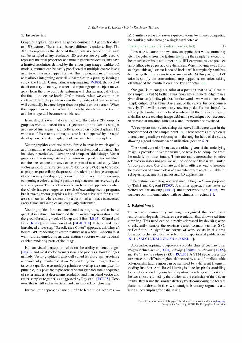
Figure 2: top: two pinchmap images [TC05]; bottom: IRT rendering

of these images retrieved from the pinchmaps paper at 256×256

resolution.

Silmaps were originally proposed to fight undersampling artifactsin shadow maps by constructing a piecewise-linear approximation tothe true shadow [SCH03]. This work was latter extended to generaltextures [Sen04] and volumetric data [KHPS07]. Silmaps eliminateblurring during texture magnification by custom-filtering colors onthe same side of the discontinuity. The algorithm supports six possi-ble configurations of the linear silhouette edges inside a pixel.

Diffusion curve textures [OBW∗08] employ a different way toachieve a resolution-independent texture representation by constru-ing an image as a solution of radiative heat transport equation. Sunet al. [SXD∗12] proposed to use an explicit form of such solutionfor closed diffusion curves as a sum of Green’s functions. Such re-duction allows a random access to the color of each texel (a fewmilliseconds per 1M texels in a typical image).

Observing that infinite resolution of vector textures is rarely re-quired, Song et al. [SWWW15] introduced a variable resolutionscheme in which an image is first partitioned into a kd-tree. Eachleaf node is then compressed with an acyclic feed-forward neuralnetwork. Such representation by vector regression functions (VRF)

allows very fast random access and filtering. VRF approximationcan cause artifacts, in particular sharp features will appear as smoothgradients in close-ups. This behavior might still be more visuallyappealing than traditional pixelization artifacts.

2.1. Comparison of IRT with Prior Art

Pinchmaps [TC05] employ the same approach as IRT by resamplingthe original raster image near the edges. A single quadratic silhouetteedge per pinchmap texel is reconstructed by bilinearly interpolatingthe four corner values that describe the edge orientation and position.

These values are then used to compute the texture coordinate offsetsthat are thence limited by a pinchmap texel size.

This method is attractive in its simplicity, always executing asingle auxiliary fetch (from a 4-channel pinchmap) for each texel.However, it does not allow edge intersections and reconstructs onlya single silhouette per pinchmap texel. Even more limiting, thepixels that are not intersected by edges will have uv offset equal to0 by design — even if there are edges in close proximity passingthrough the neighboring pixels. Accordingly, the texture coordinateoffsets across the pixels with zero and non-zero pinches will bediscontinuous. This creates artifacts that cannot be easily avoided(Figure 2).

We address these problems by storing multiple contributing sil-houette edges per texel and not limiting the magnitude of the texturecoordinate adjustment. This allows better image reconstruction andsmoother silhouettes (third order) at the cost of the more complicateddata structures (section 5.6).

In comparison with pinchmaps, silmaps [Sen04] can representsilhouette intersections. This is achieved by considering piecewise-linear segments with some mild restrictions on the edge topology(one silhouette edge per pixel side). Silmaps produce crisp edges byalways interpolating colors on the same side of the edge. To avoidfetching four corner colors that are called for by a straightforwardimplementation of this custom interpolation scheme, a clever strategyis proposed that uses a single bilinear texel lookup for 1, 2, and 4-corner cases and needs three lookups only for the 3-corner case.This compares favorably with bixels [TC04], in which a sample isevaluated by a one of the proposed ten patch functions that mightnecessitate fetching all colors at a patch boundary.

However, these custom-made interpolations make mipmappingmore complicated, requiring an explicit color blend in a shader. Anedge antialiasing would also require an extra work, making multipletexel lookups unavoidable.

In contrast, pinchmaps allow natural antialiasing and mipmappingby scaling the texture coordinate offset and we also employ a similarstrategy (section 4.2). The difference between pinchmaps and IRT inthis respect is that the expressive power of pinchmaps is somewhatdiluted by limiting the maximum magnitude of this adjustment; thisalso introduces additional frequencies pertinent to the resolution ofthe pinchmap.

All these algorithms require a pre-processing step. Pinchmapsare extracted from either a vector-based representation or a high-resolution raster image. At run-time, the appropriately downsampledraster image is used as well. The same scheme would work forsilmaps, except that for the better results the accompanying raster im-age would require special processing to recover distinct non-blurredcolors on both sides of any stored silhouettes (to facilitate custom-made interpolation at run-time). This makes this algorithm bettersuited for man-made images with pronounced edges.

Due to its less restrictive format (multiple curves per pixel, user-controlled offsets), IRT might also be suitable for some naturalimages as well (see Figures 5, 14, 12, 13). To facilitate this function-ality, we have designed an edge detection and smoothing scheme thatconverts a single raster image to a coordinated vector format (sec-

This is the authors’ version of the paper. The definitive version is available at diglib.eg.org.Eurographics Proceedings © 2016 The Eurographics Association.

A. Reshetov & D. Luebke / Infinite Resolution Textures

INPUT PRE-PROCESSING (SECTION 5)

raster image

vector graphics

RUN-TIME (SECTIONS 4 AND 6)

5.6 Create acceleration structure

5.1-5.4 Extract silhouettes

6.4 Application: sample the texture

// sample texture with the adjusted uv+duv

float4 c = tex.SampleLevel(s, uv+duv, lod);

4.1 IRT run-time: compute duv

// TC offset along the interpolated normal

duv += distance_to_rim * ni;

5.5 Renderraster image

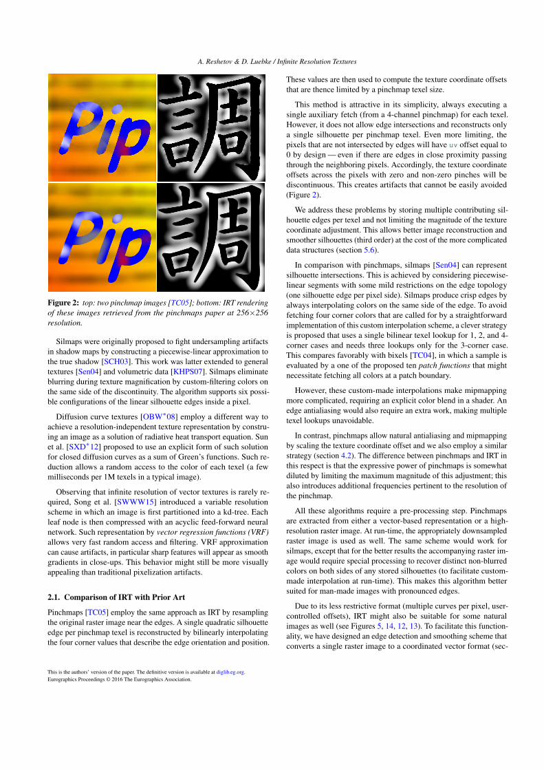
Figure 3: IRT flowchart.

tion 5). We conjecture that other texture magnification approacheswould benefit from this functionality as well.

3. Algorithm Outline

Figure 3 shows the IRT data flow, with corresponding paper sections.

To compute the texture coordinate adjustment duv in (1), we needboth a raster image and its silhouette edges. When starting froma raster image, those silhouettes have to be determined from theimage; our approach to this task is described in sections 5.1 – 5.4.Conversely, vector images do not have paired raster images as such,so one has to be rendered from the vector format at the appropriateresolution (section 5.5).

We use a grid acceleration structure to store the relevant curvedsilhouettes in the neighborhood of a given uv query (section 5.6).Note that a grid might not be an ideal structure, especially whendifferent parts of an image have vastly contrasting scales (a 2Dequivalent of the “teapot in a stadium” problem). We plan to continueexploring possible alternative approaches in this regard.

We begin by explaining our chosen way of computing theuv 7→ duv mapping, since this is at the core of IRT (section 4.1).This mapping is continuous everywhere except on edges. To avoidaliasing near the edges, we must handle such samples differently;two pertinent approaches are described in section 4.2.

Finally, we discuss performance (section 6.1) and limitations ofthe technique (6.3), then conclude with potential application areasand future work (6.4).

4. Run-Time Computations

All algorithms in this paper use the following two parameters:

• σ — the maximum distance in the RGB color spacebetween similar pixels; we use σ = 25 for all images inthis paper (for 8-bit RGB colors).

• h — an assumed size of a convolution kernel that distortsthe colors around the edges; we use 2

√2, which is the

length of the two pixel diagonals.

(2)

A sample IRT implementation is provided in Appendix A. IRTuses three types of values to compute the texture coordinate adjust-ment duv in the statement (1):

p0 = q0

q1 q2

p2 = q3

p1

b

a

θ0 θ2

n 0 n3

n b x

d0 d3

ni

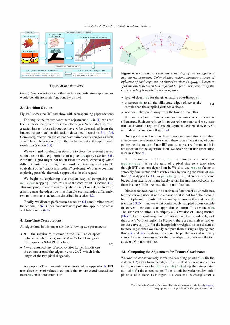
Figure 4: a continuous silhouette consisting of two straight and

two curved segments. Color shaded regions demarcate areas of

influence of each segment. At shared vertices (b,q0,q3), bisectors

split the angle between two adjacent tangent lines, separating the

corresponding truncated Voronoi regions.

• level of detail l od for the given texture coordinates uv.

• distances dc to all the silhouette edges closer to thesample than the supplied distance h above.

• vectors n i that point away from the found silhouettes.

(3)

To handle a broad class of images, we use smooth curves assilhouettes. Each curve is split into curved segments and we createtruncated Voronoi regions for such segments delineated by curve’snormals at its endpoints (Figure 4).

Our algorithm will work with any curve representation (includinga piecewise linear format) for which there is an efficient way of com-puting the distance dc. Since IRT can use any curve format and it isnot essential for the algorithm itself, we describe our implementationlater in section 5.

For mipmapped textures, l od is usually computed asl og2(p ix ra t io ), using the ratio of a pixel size to a texel size,though IRT does not depend on it. We also use reduce factor tosmoothly fuse vector and raster textures by scaling the value of duv

(line 15 in Appendix A). For p ix ra t io ≥ 1, i.e., when pixels becomebigger than texels, we immediately return the mipmapped color, sothere is a very little overhead during minification.

Distance to the curve dc is a continuous function of uv coordinates,but the curve’s normal at the closest point is not (and there couldbe multiple such points). Since we approximate the distance dc

(section 5.3.2) — and we want continuously sampled colors outsidethe curves — we can use an approximate “normal” as a value of n i.The simplest solution is to employ a 2D version of Phong normal[Pho75] by interpolating two normals defined by the side edges ofthe curve’s Voronoi region. In Figure 4, these are normals n0 and n3for the curve q0,1,2,3. For the interpolation weights, we use distancesto these edges since we already compute them during a clipping step(lines 36 and 39). By design, such an interpolated normal will varysmoothly when moving across the side edges (i.e., between the twoadjacent Voronoi regions).

4.1. Computing the Adjustment for Texture Coordinates

We want to conservatively move the sampling position uv (in thestatement 2) away from the edges. In a simplest possible implemen-tation, we just move by duv = (h - dc ) * n i along the interpolatednormal n i for the closest curve. If the sample is overlapped by multi-ple areas of influence (x in Figure 11), we sum all such adjustments,

This is the authors’ version of the paper. The definitive version is available at diglib.eg.org.Eurographics Proceedings © 2016 The Eurographics Association.

A. Reshetov & D. Luebke / Infinite Resolution Textures

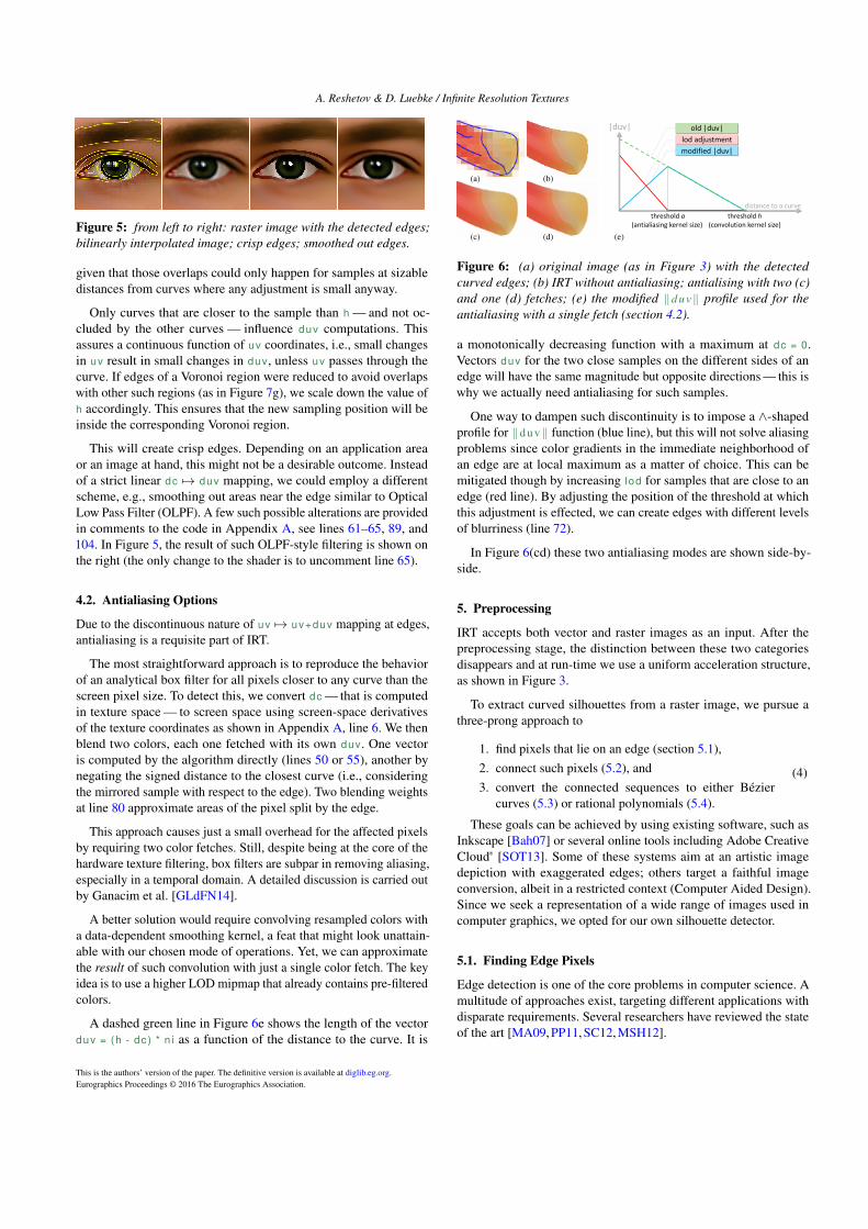
Figure 5: from left to right: raster image with the detected edges;

bilinearly interpolated image; crisp edges; smoothed out edges.

given that those overlaps could only happen for samples at sizabledistances from curves where any adjustment is small anyway.

Only curves that are closer to the sample than h — and not oc-cluded by the other curves — influence duv computations. Thisassures a continuous function of uv coordinates, i.e., small changesin uv result in small changes in duv, unless uv passes through thecurve. If edges of a Voronoi region were reduced to avoid overlapswith other such regions (as in Figure 7g), we scale down the value ofh accordingly. This ensures that the new sampling position will beinside the corresponding Voronoi region.

This will create crisp edges. Depending on an application areaor an image at hand, this might not be a desirable outcome. Insteadof a strict linear dc 7→ duv mapping, we could employ a differentscheme, e.g., smoothing out areas near the edge similar to OpticalLow Pass Filter (OLPF). A few such possible alterations are providedin comments to the code in Appendix A, see lines 61–65, 89, and104. In Figure 5, the result of such OLPF-style filtering is shown onthe right (the only change to the shader is to uncomment line 65).

4.2. Antialiasing Options

Due to the discontinuous nature of uv 7→ uv+duv mapping at edges,antialiasing is a requisite part of IRT.

The most straightforward approach is to reproduce the behaviorof an analytical box filter for all pixels closer to any curve than thescreen pixel size. To detect this, we convert dc — that is computedin texture space — to screen space using screen-space derivativesof the texture coordinates as shown in Appendix A, line 6. We thenblend two colors, each one fetched with its own duv. One vectoris computed by the algorithm directly (lines 50 or 55), another bynegating the signed distance to the closest curve (i.e., consideringthe mirrored sample with respect to the edge). Two blending weightsat line 80 approximate areas of the pixel split by the edge.

This approach causes just a small overhead for the affected pixelsby requiring two color fetches. Still, despite being at the core of thehardware texture filtering, box filters are subpar in removing aliasing,especially in a temporal domain. A detailed discussion is carried outby Ganacim et al. [GLdFN14].

A better solution would require convolving resampled colors witha data-dependent smoothing kernel, a feat that might look unattain-able with our chosen mode of operations. Yet, we can approximatethe result of such convolution with just a single color fetch. The keyidea is to use a higher LOD mipmap that already contains pre-filteredcolors.

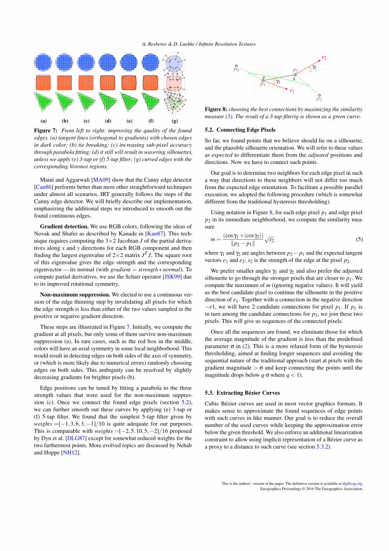
A dashed green line in Figure 6e shows the length of the vectorduv = (h - dc ) * n i as a function of the distance to the curve. It is

distance to a curve

threshold h

(convolution kernel size)

threshold a

(antialiasing kernel size)

|duv| old |duv|

lod adjustment

modified |duv|

(a) (b)

(c) (d) (e)

Figure 6: (a) original image (as in Figure 3) with the detected

curved edges; (b) IRT without antialiasing; antialising with two (c)

and one (d) fetches; (e) the modified ‖d u v‖ profile used for the

antialiasing with a single fetch (section 4.2).

a monotonically decreasing function with a maximum at dc = 0.Vectors duv for the two close samples on the different sides of anedge will have the same magnitude but opposite directions — this iswhy we actually need antialiasing for such samples.

One way to dampen such discontinuity is to impose a ∧-shapedprofile for ‖d u v‖ function (blue line), but this will not solve aliasingproblems since color gradients in the immediate neighborhood ofan edge are at local maximum as a matter of choice. This can bemitigated though by increasing l od for samples that are close to anedge (red line). By adjusting the position of the threshold at whichthis adjustment is effected, we can create edges with different levelsof blurriness (line 72).

In Figure 6(cd) these two antialiasing modes are shown side-by-side.

5. Preprocessing

IRT accepts both vector and raster images as an input. After thepreprocessing stage, the distinction between these two categoriesdisappears and at run-time we use a uniform acceleration structure,as shown in Figure 3.

To extract curved silhouettes from a raster image, we pursue athree-prong approach to

1. find pixels that lie on an edge (section 5.1),

2. connect such pixels (5.2), and

3. convert the connected sequences to either Béziercurves (5.3) or rational polynomials (5.4).

(4)

These goals can be achieved by using existing software, such asInkscape [Bah07] or several online tools including Adobe CreativeCloud® [SOT13]. Some of these systems aim at an artistic imagedepiction with exaggerated edges; others target a faithful imageconversion, albeit in a restricted context (Computer Aided Design).Since we seek a representation of a wide range of images used incomputer graphics, we opted for our own silhouette detector.

5.1. Finding Edge Pixels

Edge detection is one of the core problems in computer science. Amultitude of approaches exist, targeting different applications withdisparate requirements. Several researchers have reviewed the stateof the art [MA09, PP11, SC12, MSH12].

This is the authors’ version of the paper. The definitive version is available at diglib.eg.org.Eurographics Proceedings © 2016 The Eurographics Association.

A. Reshetov & D. Luebke / Infinite Resolution Textures

(a) (b) (c) (d) (e) (f) (g)

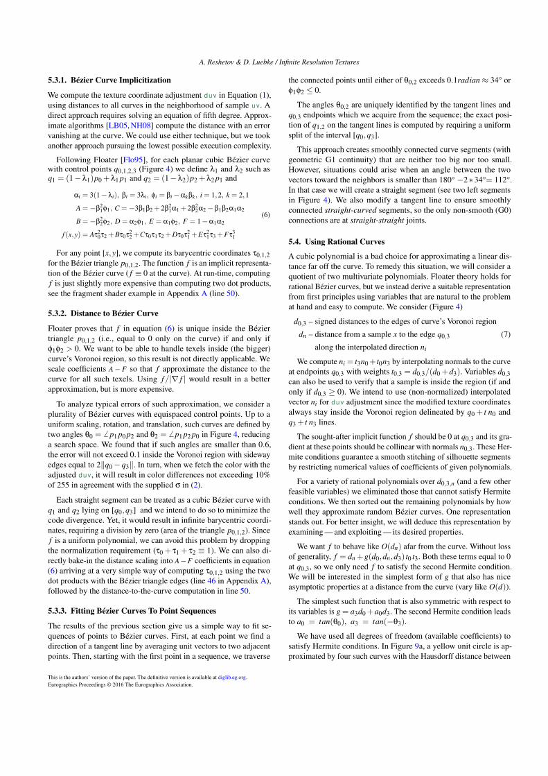
Figure 7: From left to right: improving the quality of the found

edges. (a) tangent lines (orthogonal to gradients) with chosen edges

in dark color; (b) tie breaking; (c) increasing sub-pixel accuracy

through parabola fitting; (d) it still will result in wavering silhouettes,

unless we apply (e) 3-tap or (f) 5-tap filter; (g) curved edges with the

corresponding Voronoi regions.

Maini and Aggarwali [MA09] show that the Canny edge detector[Can86] performs better than most other straightforward techniquesunder almost all scenarios. IRT generally follows the steps of theCanny edge detector. We will briefly describe our implementation,emphasizing the additional steps we introduced to smooth out thefound continuous edges.

Gradient detection. We use RGB colors, following the ideas ofNovak and Shafer as described by Kanade in [Kan87]. This tech-nique requires computing the 3×2 Jacobian J of the partial deriva-tives along x and y directions for each RGB component and thenfinding the largest eigenvalue of 2×2 matrix JT J. The square rootof this eigenvalue gives the edge strength and the correspondingeigenvector — its normal (with gradient = strength ∗ normal). Tocompute partial derivatives, we use the Scharr operator [JSK99] dueto its improved rotational symmetry.

Non-maximum suppression. We elected to use a continuous ver-sion of the edge thinning step by invalidating all pixels for whichthe edge strength is less than either of the two values sampled in thepositive or negative gradient direction.

These steps are illustrated in Figure 7. Initially, we compute thegradient at all pixels, but only some of them survive non-maximumsuppression (a). In rare cases, such as the red box in the middle,colors will have an axial symmetry in some local neighborhood. Thiswould result in detecting edges on both sides of the axis of symmetry,or (which is more likely due to numerical errors) randomly choosingedges on both sides. This ambiguity can be resolved by slightlydecreasing gradients for brighter pixels (b).

Edge positions can be tuned by fitting a parabola to the threestrength values that were used for the non-maximum suppres-sion (c). Once we connect the found edge pixels (section 5.2),we can further smooth out these curves by applying (e) 3-tap or(f) 5-tap filter. We found that the simplest 5-tap filter given byweights =[−1,3,6,3,−1]/10 is quite adequate for our purposes.This is comparable with weights =[−2,5,10,5,−2]/16 proposedby Dyn et al. [DLG87] except for somewhat reduced weights for thetwo farthermost points. More evolved topics are discussed by Nehaband Hoppe [NH12].

p0

p1

p2

p3

e1

e2

γ1

γ2

Figure 8: choosing the best connections by maximizing the similarity

measure (5). The result of a 3-tap filterig is shown as a green curve.

5.2. Connecting Edge Pixels

So far, we found points that we believe should lie on a silhouette,and the plausible silhouette orientation. We will refer to these valuesas expected to differentiate them from the adjusted positions anddirections. Now we have to connect such points.

Our goal is to determine two neighbors for each edge pixel in sucha way that directions to these neighbors will not differ too muchfrom the expected edge orientation. To facilitate a possible parallelexecution, we adopted the following procedure (which is somewhatdifferent from the traditional hysteresis thresholding).

Using notation in Figure 8, for each edge pixel p1 and edge pixelp2 in its immediate neighborhood, we compute the similarity mea-sure

m =(cosγ1 +|cosγ2|)

‖p2 − p1‖√

s2 (5)

where γ1 and γ2 are angles between p2− p1 and the expected tangentvectors e1 and e2; s2 is the strength of the edge at the pixel p2.

We prefer smaller angles γ1 and γ2 and also prefer the adjustedsilhouette to go through the stronger pixels that are closer to p1. Wecompute the maximum of m (ignoring negative values). It will yieldus the best candidate pixel to continue the silhouette in the positivedirection of e1. Together with a connection in the negative direction−e1, we will have 2 candidate connections for pixel p1. If p1 isin turn among the candidate connections for p2, we join these twopixels. This will give us sequences of the connected pixels.

Once all the sequences are found, we eliminate those for whichthe average magnitude of the gradient is less than the predefinedparameter σ in (2). This is a more relaxed form of the hysteresisthresholding, aimed at finding longer sequences and avoiding thesequential nature of the traditional approach (start at pixels with thegradient magnitude > σ and keep connecting the points until themagnitude drops below q σ where q < 1).

5.3. Extracting Bézier Curves

Cubic Bézier curves are used in most vector graphics formats. Itmakes sense to approximate the found sequences of edge pointswith such curves in like manner. Our goal is to reduce the overallnumber of the used curves while keeping the approximation errorbelow the given threshold. We also enforce an additional linearizationconstraint to allow using implicit representation of a Bézier curve asa proxy to a distance to such curve (see section 5.3.2).

This is the authors’ version of the paper. The definitive version is available at diglib.eg.org.Eurographics Proceedings © 2016 The Eurographics Association.

A. Reshetov & D. Luebke / Infinite Resolution Textures

5.3.1. Bézier Curve Implicitization

We compute the texture coordinate adjustment duv in Equation (1),using distances to all curves in the neighborhood of sample uv. Adirect approach requires solving an equation of fifth degree. Approx-imate algorithms [LB05, NH08] compute the distance with an errorvanishing at the curve. We could use either technique, but we tookanother approach pursuing the lowest possible execution complexity.

Following Floater [Flo95], for each planar cubic Bézier curvewith control points q0,1,2,3 (Figure 4) we define λ1 and λ2 such asq1 = (1−λ1)p0 +λ1 p1 and q2 = (1−λ2)p2 +λ2 p1 and

αi = 3(1−λi), βi = 3λi, φi = βi −αkβk, i = 1,2, k = 2,1

A =−β21φ1, C =−3β1β2 +2β2

1α1 +2β22α2 −β1β2α1α2

B =−β22φ2, D = α2φ1, E = α1φ2, F = 1−α1α2

f (x,y) = Aτ20τ2 +Bτ0τ2

2 +Cτ0τ1τ2 +Dτ0τ21 +Eτ2

1τ3 +Fτ31

(6)

For any point [x,y], we compute its barycentric coordinates τ0,1,2for the Bézier triangle p0,1,2. The function f is an implicit representa-tion of the Bézier curve ( f ≡ 0 at the curve). At run-time, computingf is just slightly more expensive than computing two dot products,see the fragment shader example in Appendix A (line 50).

5.3.2. Distance to Bézier Curve

Floater proves that f in equation (6) is unique inside the Béziertriangle p0,1,2 (i.e., equal to 0 only on the curve) if and only ifφ1φ2 > 0. We want to be able to handle texels inside (the bigger)curve’s Voronoi region, so this result is not directly applicable. Wescale coefficients A−F so that f approximate the distance to thecurve for all such texels. Using f/|∇ f | would result in a betterapproximation, but is more expensive.

To analyze typical errors of such approximation, we consider aplurality of Bézier curves with equispaced control points. Up to auniform scaling, rotation, and translation, such curves are defined bytwo angles θ0 = 6 p1 p0 p2 and θ2 = 6 p1 p2 p0 in Figure 4, reducinga search space. We found that if such angles are smaller than 0.6,the error will not exceed 0.1 inside the Voronoi region with sidewayedges equal to 2‖q0 −q3‖. In turn, when we fetch the color with theadjusted duv, it will result in color differences not exceeding 10%of 255 in agreement with the supplied σ in (2).

Each straight segment can be treated as a cubic Bézier curve withq1 and q2 lying on [q0,q3] and we intend to do so to minimize thecode divergence. Yet, it would result in infinite barycentric coordi-nates, requiring a division by zero (area of the triangle p0,1,2). Sincef is a uniform polynomial, we can avoid this problem by droppingthe normalization requirement (τ0 + τ1 + τ2 ≡ 1). We can also di-rectly bake-in the distance scaling into A−F coefficients in equation(6) arriving at a very simple way of computing τ0,1,2 using the twodot products with the Bézier triangle edges (line 46 in Appendix A),followed by the distance-to-the-curve computation in line 50.

5.3.3. Fitting Bézier Curves To Point Sequences

The results of the previous section give us a simple way to fit se-quences of points to Bézier curves. First, at each point we find adirection of a tangent line by averaging unit vectors to two adjacentpoints. Then, starting with the first point in a sequence, we traverse

the connected points until either of θ0,2 exceeds 0.1radian ≈ 34° orφ1φ2 ≤ 0.

The angles θ0,2 are uniquely identified by the tangent lines andq0,3 endpoints which we acquire from the sequence; the exact posi-tion of q1,2 on the tangent lines is computed by requiring a uniformsplit of the interval [q0,q3].

This approach creates smoothly connected curve segments (withgeometric G1 continuity) that are neither too big nor too small.However, situations could arise when an angle between the twovectors toward the neighbors is smaller than 180° −2∗34°= 112°.In that case we will create a straight segment (see two left segmentsin Figure 4). We also modify a tangent line to ensure smoothlyconnected straight-curved segments, so the only non-smooth (G0)connections are at straight-straight joints.

5.4. Using Rational Curves

A cubic polynomial is a bad choice for approximating a linear dis-tance far off the curve. To remedy this situation, we will consider aquotient of two multivariate polynomials. Floater theory holds forrational Bézier curves, but we instead derive a suitable representationfrom first principles using variables that are natural to the problemat hand and easy to compute. We consider (Figure 4)

d0,3 – signed distances to the edges of curve’s Voronoi region

dn – distance from a sample x to the edge q0,3

along the interpolated direction ni

(7)

We compute ni = t3n0+ t0n3 by interpolating normals to the curveat endpoints q0,3 with weights t0,3 = d0,3/(d0 +d3). Variables d0,3can also be used to verify that a sample is inside the region (if andonly if d0,3 ≥ 0). We intend to use (non-normalized) interpolatedvector ni for duv adjustment since the modified texture coordinatesalways stay inside the Voronoi region delineated by q0 + t n0 andq3 + t n3 lines.

The sought-after implicit function f should be 0 at q0,3 and its gra-dient at these points should be collinear with normals n0,3. These Her-mite conditions guarantee a smooth stitching of silhouette segmentsby restricting numerical values of coefficients of given polynomials.

For a variety of rational polynomials over d0,3,n (and a few otherfeasible variables) we eliminated those that cannot satisfy Hermiteconditions. We then sorted out the remaining polynomials by howwell they approximate random Bézier curves. One representationstands out. For better insight, we will deduce this representation byexamining — and exploiting — its desired properties.

We want f to behave like O(dn) afar from the curve. Without lossof generality, f = dn +g(d0,dn,d3) t0 t3. Both these terms equal to 0at q0,3, so we only need f to satisfy the second Hermite condition.We will be interested in the simplest form of g that also has niceasymptotic properties at a distance from the curve (vary like O(d)).

The simplest such function that is also symmetric with respect toits variables is g = a3d0 +a0d3. The second Hermite condition leadsto a0 = tan(θ0), a3 = tan(−θ3).

We have used all degrees of freedom (available coefficients) tosatisfy Hermite conditions. In Figure 9a, a yellow unit circle is ap-proximated by four such curves with the Hausdorff distance between

This is the authors’ version of the paper. The definitive version is available at diglib.eg.org.Eurographics Proceedings © 2016 The Eurographics Association.

A. Reshetov & D. Luebke / Infinite Resolution Textures

2 dof rational

0.06

(a) (b)0 5 10

0

2

4

6

8

10

3 dof rational

0.0020

(c) (d)0 5 10

0

2

4

6

8

10

Figure 9: (a) a circle approximation by four implicit rational curves

( f = x+ y− 1− x y/(x+ y) in the first quadrant); (b) contour lines for

f = (x2 + y2 − 1)/(x+ y+ 1) that approximates a unit arc exactly; (cd)

approximation by expression (8).

the two sets equal to 0.06. We can improve the approximation byadding f2 = c (d0 + d3) (t0 t3)

2 to f . This quadratic term automati-cally satisfies both Hermite conditions and asymptotically behavesas O(d0,3). We can use the constant c to fit the given points betweenq0,3. For a unit arc in the first quadrant, the resulting function

f = x+ y−1− xy (1+0.664 xy/(x+ y)2)/(x+ y) (8)

deviates from the true distance to the arc by no more than 0.2% atany distance from it, as shown in Figure 9(cd). For comparison, theHausdorff distance between a unit quarter arc and its cubic Bézier

approximation is√

71/6−2√

2/3−1 ≈ 0.03% [AKS04].

We could have approximated the arc exactly, e.g., by choos-ing f2 = c d0 d3 d1/(d0 +d3)/(d0 +d3 +1), where d1 is a distancefrom x to a line passing through q0,3. Yet, the resulting function,

f = (x2 + y2 −1)/(x+ y+1), significantly deviates from the truedistance to the arc, as can be seen in Figure 9b.

In situations when we want a sharp edge (like the two green re-gions in Figure 4 or one of the triangle vertices in Figure 7), tangentlines will be different on the two sides (G0 connectivity). Conse-quently, edges of the corresponding Voronoi regions will not beorthogonal to the tangent lines. Values of a0,3 can be then computed

as (using (·) notation for a dot product and v⊥ for an orthogonalvector) :

a0 =(q⊥10 ·q30)

(n⊥0 ·q30) (n⊥0 ·q10)

, a3 =−(q⊥23 ·q30)

(n⊥3 ·q30) (n⊥3 ·q23)

(9)

where q10 and q23 are two tangential vectors and q30 = q3 −q0.

To find the coefficient c that minimizes curve deviation froma given set of points, we solve the system of over-defined linearequations

dn +(a0d3 +a3d0) t0 t3 + c (d0 +d3) (t0 t3)2 = 0

where equation coefficients are computed at each given point (i.e.,perform a linear regression). Run-time evaluation of the distance tothe curve dc from sample uv is given in Appendix A, lines 52 – 55.

5.5. Choosing Rendering Resolution for Vector Images

When a vector image is rasterized and antialiased, a color of eachpixel is obtained by averaging all relevant subsamples. A color ofpixel p3 in Figure 11 is influenced by colors on both sides of theblue curve that intersects it. The intent of the resampling offset duv

15422

(a)

30842

(b)

41122

(c)

raster only

(d)

stored colors

(e)

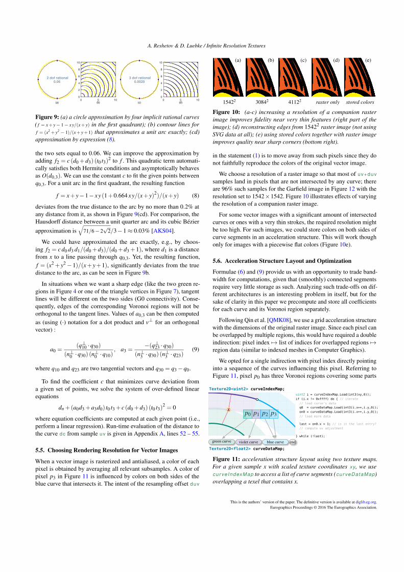
Figure 10: (a-c) increasing a resolution of a companion raster

image improves fidelity near very thin features (right part of the

image); (d) reconstructing edges from 15422 raster image (not using

SVG data at all); (e) using stored colors together with raster image

improves quality near sharp corners (bottom right).

in the statement (1) is to move away from such pixels since they donot faithfully reproduce the colors of the original vector image.

We choose a resolution of a raster image so that most of uv+duv

samples land in pixels that are not intersected by any curve; thereare 96% such samples for the Garfield image in Figure 12 with theresolution set to 1542×1542. Figure 10 illustrates effects of varyingthe resolution of a companion raster image.

For some vector images with a significant amount of intersectedcurves or ones with a very thin strokes, the required resolution mightbe too high. For such images, we could store colors on both sides ofcurve segments in an acceleration structure. This will work thoughonly for images with a piecewise flat colors (Figure 10e).

5.6. Acceleration Structure Layout and Optimization

Formulae (6) and (9) provide us with an opportunity to trade band-width for computations, given that (smoothly) connected segmentsrequire very little storage as such. Analyzing such trade-offs on dif-ferent architectures is an interesting problem in itself, but for thesake of clarity in this paper we precompute and store all coefficientsfor each curve and its Voronoi region separately.

Following Qin et al. [QMK08], we use a grid acceleration structurewith the dimensions of the original raster image. Since each pixel canbe overlapped by multiple regions, this would have required a doubleindirection: pixel index 7→ list of indices for overlapped regions 7→region data (similar to indexed meshes in Computer Graphics).

We opted for a single indirection with pixel index directly pointinginto a sequence of the curves influencing this pixel. Referring toFigure 11, pixel p0 has three Voronoi regions covering some parts

p0 p1 p2 p3x

green curve violet curve blue curve end

Texture2D<uint2> curveIndexMap;

Texture2D<float2> curveDataMap;

uint2 i = curveIndexMap.Load(int3(xy,0));

if (i.x != 0xffff) do { // iterate

// load curve’s data

q0 = curveDataMap.Load(int3(i.x++,i.y,0));

on0 = curveDataMap.Load(int3(i.x++,i.y,0));

// load more data...

last = on0.x > 1; // is it the last entry?

// compute uv adjustment...

} while (!last);

Figure 11: acceleration structure layout using two texture maps.

For a given sample x with scaled texture coordinates xy, we use

cur ve IndexMap to access a list of curve segments (cur veDataMap)

overlapping a texel that contains x.

This is the authors’ version of the paper. The definitive version is available at diglib.eg.org.Eurographics Proceedings © 2016 The Eurographics Association.

A. Reshetov & D. Luebke / Infinite Resolution Textures

of it and its index points into the start of the sequence of three suchcurves. Pixel p1 is overlapped by only violet and blue regions and itpoints into the second entry in the same sequence, while p2,3 sharethe blue region at the end of the sequence. At run time, we iterateover all corresponding curves until the end-of-the-sequence flag isread (see do ...whi le loop at line 21 in Appendix A).

To minimize the overlap of areas of influence for each curve (asfor sample x in Figure 11), we construct a Voronoi diagram for super-sampled edges and then consider intersections of normals at curves’endpoints with such a diagram to produce side edges for truncatedVoronoi regions. We clip such vectors if their length exceeds thesupplied parameter h in (2) and (optionally) reduce them for weakedges as defined by the gradient magnitude during the edge detectionstep (section 5.1). If the intersection of these two vectors for eachregion is closer to q0,3 than their assigned length, we reduce thislength to exclude the intersection from the area of influence andavoid potential division by zero during the run-time computation(line 37 in Appendix A). By linearly interpolating the found edgevectors — considering both positive and negative directions — wewill get an area of influence for a particular curve (line 58). Suchareas will contain points that are closer to the given curve than toany other (as in Figure 7g). Small overlaps are still possible and wehandle them by summing the corresponding duv offsets so not toimpair duv continuity (line 86).

6. Discussion

IRT combines the best traits of vector and raster textures in a unifiedarrangement. It smoothly blends vector and raster representationsto exploit the pre-filtered accommodating properties of the tradi-tional textures at farther distances. This blending does not incur anyadditional penalty, besides computing the mipmap level. Thus, theinfinite resolution textures are only slightly more expensive thantraditional mipmapped textures for distant objects and exhibit rea-sonable performance for close-ups (section 6.1).

IRT textures differ from traditional textures at closer distances,revealing crisp edges that hopefully agree with human intuition.There are clearly limits to such detail hallucination (section 6.3).

6.1. Performance

By creatively using hardware not originally designed for vectorgraphics per se, GPU-accelerated methods for vector textures [KB12,GLdFN14] achieve rendering times of 20+ milliseconds per 1Mtexels. This works well when the whole image has to be rendered,since certain operations are amortized over the whole image.

Our goal is to complement such methods, targeting resource con-sumption by games with random texture sampling, rather than re-source creation. We measured the performance of our algorithm ona discrete GeForceTM GTX 980 using a Direct3D 11 viewer.

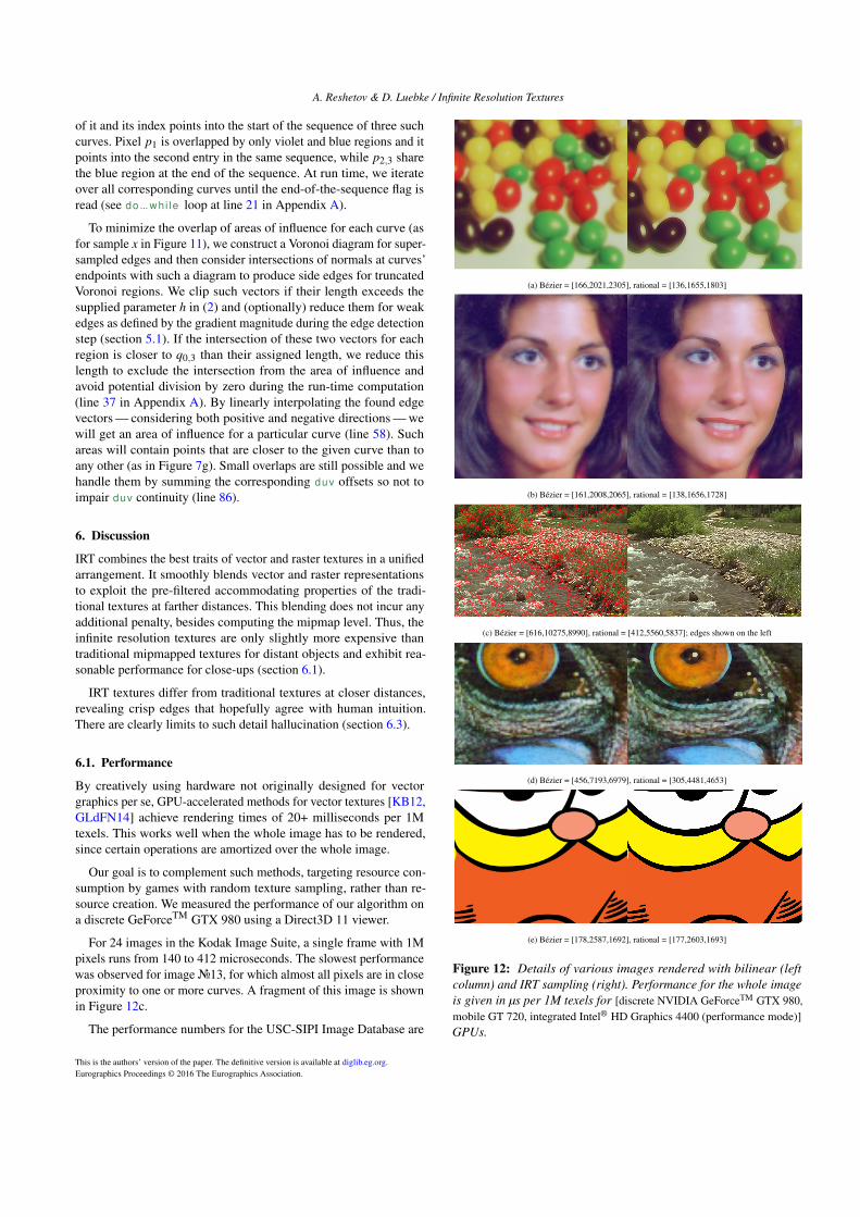
For 24 images in the Kodak Image Suite, a single frame with 1Mpixels runs from 140 to 412 microseconds. The slowest performancewas observed for image№13, for which almost all pixels are in closeproximity to one or more curves. A fragment of this image is shownin Figure 12c.

The performance numbers for the USC-SIPI Image Database are

(a) Bézier = [166,2021,2305], rational = [136,1655,1803]

(b) Bézier = [161,2008,2065], rational = [138,1656,1728]

(c) Bézier = [616,10275,8990], rational = [412,5560,5837]; edges shown on the left

(d) Bézier = [456,7193,6979], rational = [305,4481,4653]

(e) Bézier = [178,2587,1692], rational = [177,2603,1693]

Figure 12: Details of various images rendered with bilinear (left

column) and IRT sampling (right). Performance for the whole image

is given in µs per 1M texels for [discrete NVIDIA GeForceTM GTX 980,mobile GT 720, integrated Intel® HD Graphics 4400 (performance mode)]GPUs.

This is the authors’ version of the paper. The definitive version is available at diglib.eg.org.Eurographics Proceedings © 2016 The Eurographics Association.

A. Reshetov & D. Luebke / Infinite Resolution Textures

13.9

12.011.5

18.9

13.0

11.7

14.9

12.6 12.4

17.2 17.216.9

TX0 IRT single map TX∞

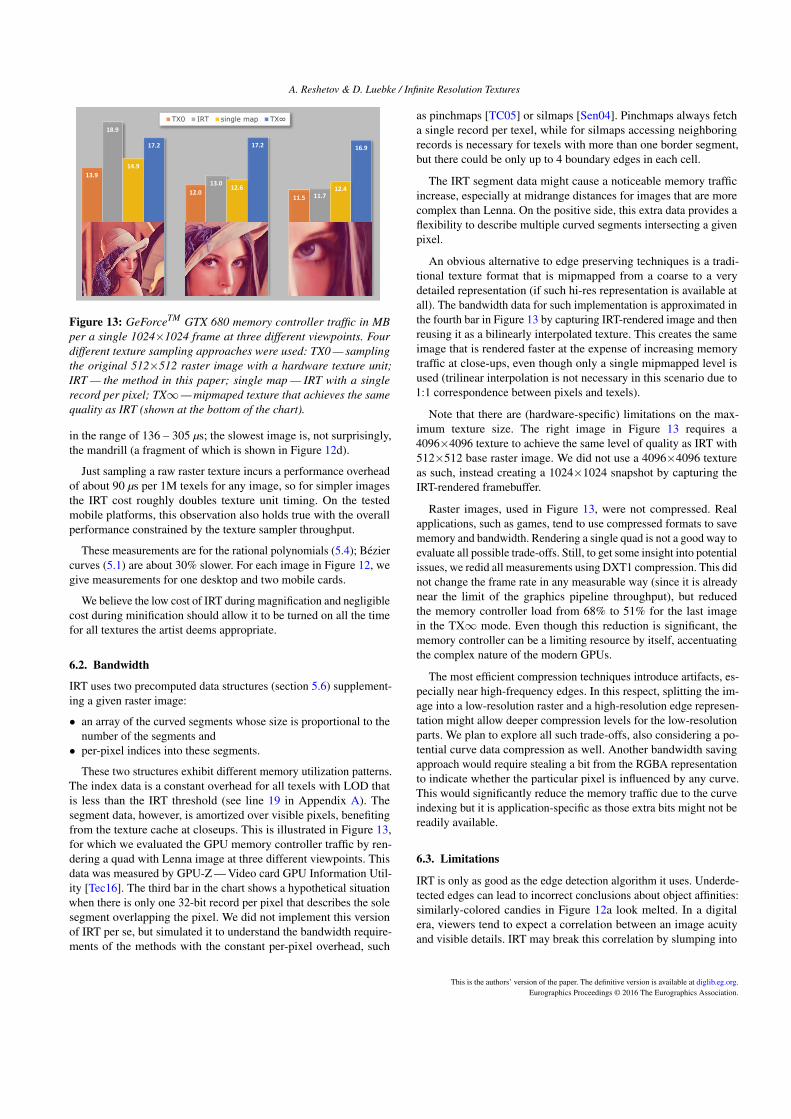
Figure 13: GeForceTM GTX 680 memory controller traffic in MB

per a single 1024×1024 frame at three different viewpoints. Four

different texture sampling approaches were used: TX0 — sampling

the original 512×512 raster image with a hardware texture unit;

IRT — the method in this paper; single map — IRT with a single

record per pixel; TX∞— mipmaped texture that achieves the same

quality as IRT (shown at the bottom of the chart).

in the range of 136 – 305 µs; the slowest image is, not surprisingly,the mandrill (a fragment of which is shown in Figure 12d).

Just sampling a raw raster texture incurs a performance overheadof about 90 µs per 1M texels for any image, so for simpler imagesthe IRT cost roughly doubles texture unit timing. On the testedmobile platforms, this observation also holds true with the overallperformance constrained by the texture sampler throughput.

These measurements are for the rational polynomials (5.4); Béziercurves (5.1) are about 30% slower. For each image in Figure 12, wegive measurements for one desktop and two mobile cards.

We believe the low cost of IRT during magnification and negligiblecost during minification should allow it to be turned on all the timefor all textures the artist deems appropriate.

6.2. Bandwidth

IRT uses two precomputed data structures (section 5.6) supplement-ing a given raster image:

• an array of the curved segments whose size is proportional to thenumber of the segments and

• per-pixel indices into these segments.

These two structures exhibit different memory utilization patterns.The index data is a constant overhead for all texels with LOD thatis less than the IRT threshold (see line 19 in Appendix A). Thesegment data, however, is amortized over visible pixels, benefitingfrom the texture cache at closeups. This is illustrated in Figure 13,for which we evaluated the GPU memory controller traffic by ren-dering a quad with Lenna image at three different viewpoints. Thisdata was measured by GPU-Z — Video card GPU Information Util-ity [Tec16]. The third bar in the chart shows a hypothetical situationwhen there is only one 32-bit record per pixel that describes the solesegment overlapping the pixel. We did not implement this versionof IRT per se, but simulated it to understand the bandwidth require-ments of the methods with the constant per-pixel overhead, such

as pinchmaps [TC05] or silmaps [Sen04]. Pinchmaps always fetcha single record per texel, while for silmaps accessing neighboringrecords is necessary for texels with more than one border segment,but there could be only up to 4 boundary edges in each cell.

The IRT segment data might cause a noticeable memory trafficincrease, especially at midrange distances for images that are morecomplex than Lenna. On the positive side, this extra data provides aflexibility to describe multiple curved segments intersecting a givenpixel.

An obvious alternative to edge preserving techniques is a tradi-tional texture format that is mipmapped from a coarse to a verydetailed representation (if such hi-res representation is available atall). The bandwidth data for such implementation is approximated inthe fourth bar in Figure 13 by capturing IRT-rendered image and thenreusing it as a bilinearly interpolated texture. This creates the sameimage that is rendered faster at the expense of increasing memorytraffic at close-ups, even though only a single mipmapped level isused (trilinear interpolation is not necessary in this scenario due to1:1 correspondence between pixels and texels).

Note that there are (hardware-specific) limitations on the max-imum texture size. The right image in Figure 13 requires a4096×4096 texture to achieve the same level of quality as IRT with512×512 base raster image. We did not use a 4096×4096 textureas such, instead creating a 1024×1024 snapshot by capturing theIRT-rendered framebuffer.

Raster images, used in Figure 13, were not compressed. Realapplications, such as games, tend to use compressed formats to savememory and bandwidth. Rendering a single quad is not a good way toevaluate all possible trade-offs. Still, to get some insight into potentialissues, we redid all measurements using DXT1 compression. This didnot change the frame rate in any measurable way (since it is alreadynear the limit of the graphics pipeline throughput), but reducedthe memory controller load from 68% to 51% for the last imagein the TX∞ mode. Even though this reduction is significant, thememory controller can be a limiting resource by itself, accentuatingthe complex nature of the modern GPUs.

The most efficient compression techniques introduce artifacts, es-pecially near high-frequency edges. In this respect, splitting the im-age into a low-resolution raster and a high-resolution edge represen-tation might allow deeper compression levels for the low-resolutionparts. We plan to explore all such trade-offs, also considering a po-tential curve data compression as well. Another bandwidth savingapproach would require stealing a bit from the RGBA representationto indicate whether the particular pixel is influenced by any curve.This would significantly reduce the memory traffic due to the curveindexing but it is application-specific as those extra bits might not bereadily available.

6.3. Limitations

IRT is only as good as the edge detection algorithm it uses. Underde-tected edges can lead to incorrect conclusions about object affinities:similarly-colored candies in Figure 12a look melted. In a digitalera, viewers tend to expect a correlation between an image acuityand visible details. IRT may break this correlation by slumping into

This is the authors’ version of the paper. The definitive version is available at diglib.eg.org.Eurographics Proceedings © 2016 The Eurographics Association.

A. Reshetov & D. Luebke / Infinite Resolution Textures

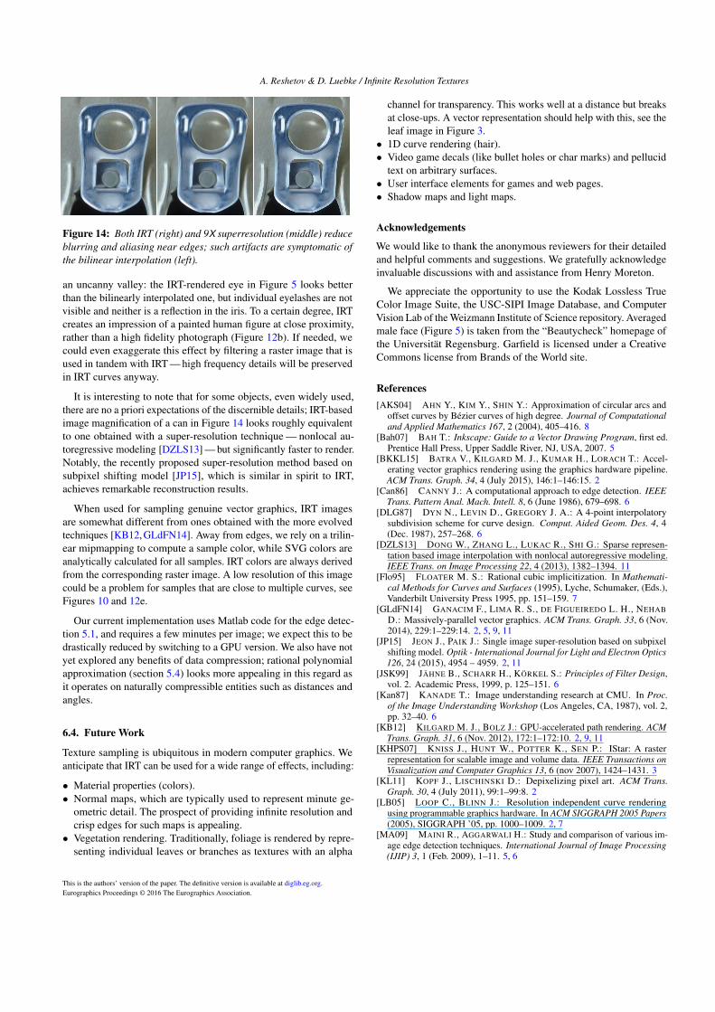
Figure 14: Both IRT (right) and 9X superresolution (middle) reduce

blurring and aliasing near edges; such artifacts are symptomatic of

the bilinear interpolation (left).

an uncanny valley: the IRT-rendered eye in Figure 5 looks betterthan the bilinearly interpolated one, but individual eyelashes are notvisible and neither is a reflection in the iris. To a certain degree, IRTcreates an impression of a painted human figure at close proximity,rather than a high fidelity photograph (Figure 12b). If needed, wecould even exaggerate this effect by filtering a raster image that isused in tandem with IRT — high frequency details will be preservedin IRT curves anyway.

It is interesting to note that for some objects, even widely used,there are no a priori expectations of the discernible details; IRT-basedimage magnification of a can in Figure 14 looks roughly equivalentto one obtained with a super-resolution technique — nonlocal au-toregressive modeling [DZLS13] — but significantly faster to render.Notably, the recently proposed super-resolution method based onsubpixel shifting model [JP15], which is similar in spirit to IRT,achieves remarkable reconstruction results.

When used for sampling genuine vector graphics, IRT imagesare somewhat different from ones obtained with the more evolvedtechniques [KB12, GLdFN14]. Away from edges, we rely on a trilin-ear mipmapping to compute a sample color, while SVG colors areanalytically calculated for all samples. IRT colors are always derivedfrom the corresponding raster image. A low resolution of this imagecould be a problem for samples that are close to multiple curves, seeFigures 10 and 12e.

Our current implementation uses Matlab code for the edge detec-tion 5.1, and requires a few minutes per image; we expect this to bedrastically reduced by switching to a GPU version. We also have notyet explored any benefits of data compression; rational polynomialapproximation (section 5.4) looks more appealing in this regard asit operates on naturally compressible entities such as distances andangles.

6.4. Future Work

Texture sampling is ubiquitous in modern computer graphics. Weanticipate that IRT can be used for a wide range of effects, including:

• Material properties (colors).• Normal maps, which are typically used to represent minute ge-

ometric detail. The prospect of providing infinite resolution andcrisp edges for such maps is appealing.

• Vegetation rendering. Traditionally, foliage is rendered by repre-senting individual leaves or branches as textures with an alpha

channel for transparency. This works well at a distance but breaksat close-ups. A vector representation should help with this, see theleaf image in Figure 3.

• 1D curve rendering (hair).• Video game decals (like bullet holes or char marks) and pellucid

text on arbitrary surfaces.• User interface elements for games and web pages.• Shadow maps and light maps.

Acknowledgements

We would like to thank the anonymous reviewers for their detailedand helpful comments and suggestions. We gratefully acknowledgeinvaluable discussions with and assistance from Henry Moreton.

We appreciate the opportunity to use the Kodak Lossless TrueColor Image Suite, the USC-SIPI Image Database, and ComputerVision Lab of the Weizmann Institute of Science repository. Averagedmale face (Figure 5) is taken from the “Beautycheck” homepage ofthe Universität Regensburg. Garfield is licensed under a CreativeCommons license from Brands of the World site.

References

[AKS04] AHN Y., KIM Y., SHIN Y.: Approximation of circular arcs andoffset curves by Bézier curves of high degree. Journal of Computational

and Applied Mathematics 167, 2 (2004), 405–416. 8[Bah07] BAH T.: Inkscape: Guide to a Vector Drawing Program, first ed.

Prentice Hall Press, Upper Saddle River, NJ, USA, 2007. 5[BKKL15] BATRA V., KILGARD M. J., KUMAR H., LORACH T.: Accel-

erating vector graphics rendering using the graphics hardware pipeline.ACM Trans. Graph. 34, 4 (July 2015), 146:1–146:15. 2

[Can86] CANNY J.: A computational approach to edge detection. IEEE

Trans. Pattern Anal. Mach. Intell. 8, 6 (June 1986), 679–698. 6[DLG87] DYN N., LEVIN D., GREGORY J. A.: A 4-point interpolatory

subdivision scheme for curve design. Comput. Aided Geom. Des. 4, 4(Dec. 1987), 257–268. 6

[DZLS13] DONG W., ZHANG L., LUKAC R., SHI G.: Sparse represen-tation based image interpolation with nonlocal autoregressive modeling.IEEE Trans. on Image Processing 22, 4 (2013), 1382–1394. 11

[Flo95] FLOATER M. S.: Rational cubic implicitization. In Mathemati-

cal Methods for Curves and Surfaces (1995), Lyche, Schumaker, (Eds.),Vanderbilt University Press 1995, pp. 151–159. 7

[GLdFN14] GANACIM F., LIMA R. S., DE FIGUEIREDO L. H., NEHAB

D.: Massively-parallel vector graphics. ACM Trans. Graph. 33, 6 (Nov.2014), 229:1–229:14. 2, 5, 9, 11

[JP15] JEON J., PAIK J.: Single image super-resolution based on subpixelshifting model. Optik - International Journal for Light and Electron Optics

126, 24 (2015), 4954 – 4959. 2, 11[JSK99] JÄHNE B., SCHARR H., KÖRKEL S.: Principles of Filter Design,

vol. 2. Academic Press, 1999, p. 125–151. 6[Kan87] KANADE T.: Image understanding research at CMU. In Proc.

of the Image Understanding Workshop (Los Angeles, CA, 1987), vol. 2,pp. 32–40. 6

[KB12] KILGARD M. J., BOLZ J.: GPU-accelerated path rendering. ACM

Trans. Graph. 31, 6 (Nov. 2012), 172:1–172:10. 2, 9, 11[KHPS07] KNISS J., HUNT W., POTTER K., SEN P.: IStar: A raster

representation for scalable image and volume data. IEEE Transactions on

Visualization and Computer Graphics 13, 6 (nov 2007), 1424–1431. 3[KL11] KOPF J., LISCHINSKI D.: Depixelizing pixel art. ACM Trans.

Graph. 30, 4 (July 2011), 99:1–99:8. 2[LB05] LOOP C., BLINN J.: Resolution independent curve rendering

using programmable graphics hardware. In ACM SIGGRAPH 2005 Papers

(2005), SIGGRAPH ’05, pp. 1000–1009. 2, 7[MA09] MAINI R., AGGARWALI H.: Study and comparison of various im-

age edge detection techniques. International Journal of Image Processing

(IJIP) 3, 1 (Feb. 2009), 1–11. 5, 6

This is the authors’ version of the paper. The definitive version is available at diglib.eg.org.Eurographics Proceedings © 2016 The Eurographics Association.

A. Reshetov & D. Luebke / Infinite Resolution Textures

[MSH12] MITTAL A., SOFAT S., HANCOCK E. R.: Detection of edgesin color images: A review and evaluative comparison of state-of-the-arttechniques. In Proc. Autonomous and Intelligent Systems (AIS) 2012

(2012), pp. 250–259. 5[NH08] NEHAB D., HOPPE H.: Random-access rendering of general

vector graphics. ACM Trans. Graph. 27, 5 (Dec. 2008), 135:1–135:10. 7[NH12] NEHAB D., HOPPE H.: A fresh look at generalized sampling.

Foundations and Trends in Computer Graphics and Vision 8, 1 (2012),1–84. 6

[OBW∗08] ORZAN A., BOUSSEAU A., WINNEMÖLLER H., BARLA P.,THOLLOT J., SALESIN D.: Diffusion curves: A vector representation forsmooth-shaded images. ACM Trans. Graph. 27, 3 (2008), 1–8. SpecialIssue: SIGGRAPH 2008. 3

[Pho75] PHONG B. T.: Illumination for computer generated pictures.Commun. ACM 18, 6 (June 1975), 311–317. 4

[PP11] PAPARI G., PETKOV N.: Review article: Edge and line orientedcontour detection: State of the art. Image Vision Comput. 29, 2-3 (Feb.2011), 79–103. 5

[QMK08] QIN Z., MCCOOL M. D., KAPLAN C.: Precise vector texturesfor real-time 3D rendering. In Proc. of the 2008 Symposium on Interactive

3D Graphics and Games (2008), I3D ’08, pp. 199–206. 8[RCL05] RAY N., CAVIN X., LÉVY B.: Vector texture maps on the

GPU. Tech. rep., Laboratoire Lorrain de Recherche en Informatique etses Applications, 2005. 2

[Res12] RESHETOV A.: Reducing aliasing artifacts through resampling.In Proc. of the Fourth ACM SIGGRAPH/Eurographics Conf. on High-

Performance Graphics (2012), EGGH-HPG ’12, pp. 77–86. 2[SC12] SHRIVAKSHAN G. T., CHANDRASEKAR C.: A comparison of

various edge detection techniques used in image processing. IJCSI Press.5

[SCH03] SEN P., CAMMARANO M., HANRAHAN P.: Shadow silhouettemaps. In ACM SIGGRAPH 2003 Papers (2003), SIGGRAPH ’03, pp. 521–526. 3

[Sen04] SEN P.: Silhouette maps for improved texture magnification. InProc. of the ACM SIGGRAPH/Eurographics Conf. on Graphics Hardware

(2004), HWWS ’04, pp. 65–73. 2, 3, 10[Sha73] SHAPLEY R. M.TOLHURST D. J.: Edge detectors in human

vision. The Journal of Physiology 229, 1 (1973), 165–183. 2[SOT13] SMITH J., OSBORN J., TEAM A. C.: Adobe Creative Cloud

Design Tools Digital Classroom, 1st ed. Wiley Publishing, 2013. 5[SWWW15] SONG Y., WANG J., WEI L.-Y., WANG W.: Vector regres-

sion functions for texture compression. ACM TOG 35, 1 (2015). 3[SXD∗12] SUN X., XIE G., DONG Y., LIN S., XU W., WANG W., TONG

X., GUO B.: Diffusion curve textures for resolution independent texturemapping. ACM Trans. Graph. 31, 4 (July 2012), 74:1–74:9. 2, 3

[TC04] TUMBLIN J., CHOUDHURY P.: Bixels: Picture Samples with SharpEmbedded Boundaries. Eurographics Workshop on Rendering (2004). 2,3

[TC05] TARINI M., CIGNONI P.: Pinchmaps: textures with customizablediscontinuities. Comput. Graph. Forum 24, 3 (2005), 557–568. 2, 3, 10

[Tec16] TECHPOWERUP: GPU-Z Video card GPU Information Utility,2016. URL: https://www.techpowerup.com/gpuz. 10

[Wil83] WILLIAMS L.: Pyramidal parametrics. SIGGRAPH Comput.

Graph. 17, 3 (July 1983), 1–11. 2

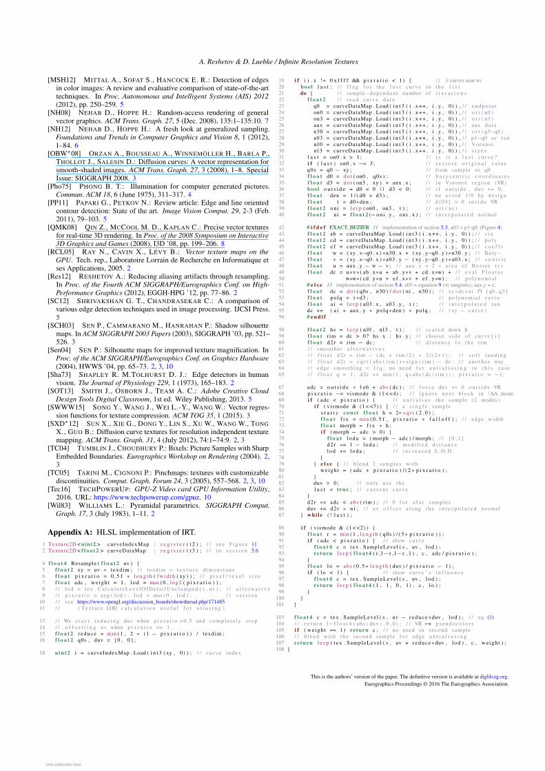
Appendix A: HLSL implementation of IRT.1 Texture2D < uint2 > curveIndexMap : r e g i s t e r ( t 2 ) ; / / s e e F i g u r e 112 Texture2D < f l o a t 2 > curveDataMap : r e g i s t e r ( t 3 ) ; / / i n s e c t i o n 5.6

4 f l o a t 4 Resample ( f l o a t 2 uv ) {5 f l o a t 2 xy = uv * texd im ; / / t exd im = t e x t u r e d i m e n s i o n s6 f l o a t p i x r a t i o = 0 . 5 f * l e n g t h ( f w i d t h ( xy ) ) ; / / p i x e l / t e x e l s i z e7 f l o a t adc , we ig h t = 1 , l o d = max ( 0 , l og2 ( p i x r a t i o ) ) ;8 / / l o d = t e x . C a l c u l a t e L e v e l O f D e t a i l U n c l a m p e d ( s , uv ) ; / / a l t e r n a t i v e9 / / p i x r a t i o = exp ( l o d ) ; l o d = max ( 0 , l o d ) ; / / v e r s i o n

10 / / s e e https://www.opengl.org/discussion_boards/showthread.php/17148511 / / ( T e x t u r e LOD c a l c u l a t i o n u s e f u l f o r a t l a s i n g )

13 / / We s t a r t r e d u c i n g duv when p i x r a t i o >0 .5 and c o m p l e t e l y s t o p14 / / o f f s e t t i n g uv when p i x r a t i o >= 1 .15 f l o a t 2 r e d u c e = min ( 1 , 2 * (1 − p i x r a t i o ) ) / t exd im ;16 f l o a t 2 q0s , duv = {0 , 0 } ;

18 u i n t 2 i = curveIndexMap . Load ( i n t 3 ( xy , 0 ) ) ; / / c u r v e i n d e x

19 i f ( i . x != 0 x f f f f && p i x r a t i o < 1) { / / ∃ curves near uv20 bool l a s t ; / / f l a g f o r t h e l a s t c u r v e i n t h e l i s t21 do { / / sample−d e p e n d e n t number o f i t e r a t i o n s22 f l o a t 2 / / r e a d c u r v e d a t a23 q0 = curveDataMap . Load ( i n t 3 ( i . x ++ , i . y , 0 ) ) , / / e n d p o i n t24 on0 = curveDataMap . Load ( i n t 3 ( i . x ++ , i . y , 0 ) ) , / / o r t ( n0 )25 on3 = curveDataMap . Load ( i n t 3 ( i . x ++ , i . y , 0 ) ) , / / o r t ( n3 )26 aux = curveDataMap . Load ( i n t 3 ( i . x ++ , i . y , 0 ) ) , / / aux d a t a27 n30 = curveDataMap . Load ( i n t 3 ( i . x ++ , i . y , 0 ) ) , / / o r t ( q3−q0 )28 a03 = curveDataMap . Load ( i n t 3 ( i . x ++ , i . y , 0 ) ) , / / p1−q0 or t a n29 n l 0 = curveDataMap . Load ( i n t 3 ( i . x ++ , i . y , 0 ) ) , / / Voronoi30 n l 3 = curveDataMap . Load ( i n t 3 ( i . x ++ , i . y , 0 ) ) ; / / s i z e s31 l a s t = on0 . x > 1 ; / / i s i t a l a s t c u r v e ?32 i f ( l a s t ) on0 . x −= 3 ; / / r e s t o r e o r i g i n a l v a l u e33 q0s = q0 − xy ; / / from sample t o q034 f l o a t d0 = d o t ( on0 , q0s ) ; / / b a r y c e n t r i c c o o r d i n a t e s35 f l o a t d3 = d o t ( on3 , xy ) + aux . x ; / / i n Voronoi r e g i o n (VR)36 bool o u t s i d e = d0 < 0 | | d3 < 0 ; / / i f o u t s i d e , duv += 0 ;37 f l o a t den = 1 / ( d0 + d3 ) ; / / we a v o i d 1 / 0 by d e s i g n38 f l o a t t = d0* den ; / / d {03} > 0 i n s i d e VR39 f l o a t 2 o n i = l e r p ( on0 , on3 , t ) ; / / o r t ( n i )40 f l o a t 2 n i = f l o a t 2 (−o n i . y , o n i . x ) ; / / i n t e r p o l a t e d normal

42 # i f d e f EXACT_BEZIER / / implementation of section 5.3; a03 = p1-q0; (Figure 4)43 f l o a t 2 ab = curveDataMap . Load ( i n t 3 ( i . x ++ , i . y , 0 ) ) ; / / s i x44 f l o a t 2 cd = curveDataMap . Load ( i n t 3 ( i . x ++ , i . y , 0 ) ) ; / / po ly45 f l o a t 2 e f = curveDataMap . Load ( i n t 3 ( i . x ++ , i . y , 0 ) ) ; / / c o e f f s46 f l o a t w = ( xy . x−q0 . x ) * n30 . x + ( xy . y−q0 . y ) *n30 . y ; / / Bary−47 f l o a t v = ( xy . x−q0 . x ) * a03 . y − ( xy . y−q0 . y ) * a03 . x ; / / c e n t r i c48 f l o a t u = aux . y − w − v ; / / aux . y = 2 * a r e a o f B e z i e r t r i49 f l o a t dc = u*v *( ab . x*u + ab . y*v + cd . x*w) + / / e v a l F l o a t e r50 w*w*( cd . y*u + e f . x*v + e f . y*w) ; / / p o l y n o m i a l51 # e l s e / / implementation of section 5.4; a03 = equation 9 (≈ tangents); aux.y = c;52 f l o a t dc = d o t ( q0s , n30 ) / d o t ( n i , n30 ) ; / / xy+dc * n i ∩ [ q0 , q3 ]53 f l o a t po lq = t *d3 ; / / p o l y n o m i a l r a t i o54 f l o a t a i = l e r p ( a03 . x , a03 . y , t ) ; / / i n t e r p o l a t e d t a n55 dc += ( a i + aux . y * po lq * den ) * po lq ; / / | xy − c u r v e |56 # e n d i f

58 f l o a t 2 hs = l e r p ( nl0 , nl3 , t ) ; / / s c a l e d down h59 f l o a t r im = dc > 0? hs . x : hs . y ; / / choose s i d e o f c u r v e [ i ]60 f l o a t d2r = rim − dc ; / / d i s t a n c e t o t h e r im61 / / smoo the r a l t e r n a t i v e s62 / / f l o a t d2r = r im − ( dc + rim / 2 ) * 2 / ( 2 + 1 ) ; / / s o f t l a n d i n g63 / / f l o a t d2r = s q r t ( abs ( r im ) ) * s i g n ( r im ) − dc ; / / a n o t h e r way64 / / edge smooth ing = 1 / q ; no need f o r a n t i a l i a s i n g i n t h i s c a s e65 / / f l o a t q = 1 ; d2r *= min ( 1 , q* abs ( dc / r im ) ) ; p i x r a t i o = −1;

67 adc = o u t s i d e * 1 e6 + abs ( dc ) ; / / f o r c e duv += 0 o u t s i d e VR68 p i x r a t i o −= vismode & (1 < <4) ; / / i g n o r e n e x t b l o c k i n !AA mode69 i f ( adc < p i x r a t i o ) { / / a n t i a l i a s t h e sample (2 modes )70 i f ( vismode & (1 < <7) ) { / / a s i n g l e sample71 s t a t i c c o n s t f l o a t h = 2* s q r t ( 2 . 0 ) ;72 f l o a t f i x = min ( 0 . 5 f , p i x r a t i o * f a l l o f f ) ; / / edge wid th73 f l o a t morph = f i x * h ;74 i f ( morph − adc > 0) {75 f l o a t l o d a = ( morph − adc ) / morph ; / / [ 0 , 1 ]76 d2r *= 1 − l o d a ; / / m o d i f i e d d i s t a n c e77 l o d += l o d a ; / / i n c r e a s e d L .O.D.78 }79 } e l s e { / / b l e n d 2 samples wi th80 w e i gh t = ( adc + p i x r a t i o ) / ( 2 * p i x r a t i o ) ;81 }82 duv = 0 ; / / on ly use t h e83 l a s t = t ru e ; / / c u r r e n t c u r v e84 }85 d2r *= adc < abs ( r im ) ; / / 0 f o r a f a r samples86 duv += d2r * n i ; / / uv o f f s e t a l o n g t h e i n t e r p o l a t e d normal87 } whi le ( ! l a s t ) ;

89 i f ( vismode & (1 < <2) ) {90 f l o a t r = min ( 1 , l e n g t h ( q0s ) / ( 5 * p i x r a t i o ) ) ;91 i f ( adc < p i x r a t i o ) { / / show c u r v e92 f l o a t 4 c = t e x . SampleLevel ( s , uv , l o d ) ;93 re turn l e r p ( f l o a t 4 ( r ,1− r ,1− r , 1 ) , c , adc / p i x r a t i o ) ;94 }95 f l o a t l o = abs ( 0 . 5 * l e n g t h ( duv ) / p i x r a t i o − 1) ;96 i f ( l o < 1) { / / show curve ’ s i n f l u e n c e97 f l o a t 4 c = t e x . SampleLevel ( s , uv , l o d ) ;98 re turn l e r p ( f l o a t 4 ( 1 , 1 , 0 , 1 ) , c , l o ) ;99 }

100 }101 }

103 f l o a t 4 c = t e x . SampleLevel ( s , uv − r e d u c e *duv , l o d ) ; / / eq (1)104 / / r e t u r n 1− f l o a t 4 ( abs ( duv ) , 0 , 0 ) ; / / VR 7→ p s e u d o c o l o r s105 i f ( we ig h t == 1) re turn c ; / / no need i n second sample106 / / b l e n d wi th t h e second sample f o r edge a n t i a l i a s i n g107 re turn l e r p ( t e x . SampleLevel ( s , uv + r e d u c e *duv , l o d ) , c , w e i gh t ) ;108 }

This is the authors’ version of the paper. The definitive version is available at diglib.eg.org.Eurographics Proceedings © 2016 The Eurographics Association.

View publication statsView publication stats