inflation expectations and consumer spending at … expectations and consumer spending at the zero...

Inflation Expectations and Consumer Spending at the Zero Bound: Micro Evidence Hibiki Ichiue* [email protected] Shusaku Nishiguchi** [email protected]

No.13-E-11 July 2013

Bank of Japan 2-1-1 Nihonbashi-Hongokucho, Chuo-ku, Tokyo 103-0021, Japan

* Monetary Affairs Department ** Monetary Affairs Department

Papers in the Bank of Japan Working Paper Series are circulated in order to stimulate discussion and comments. Views expressed are those of authors and do not necessarily reflect those of the Bank. If you have any comment or question on the working paper series, please contact each author.

When making a copy or reproduction of the content for commercial purposes, please contact the Public Relations Department ([email protected]) at the Bank in advance to request permission. When making a copy or reproduction, the source, Bank of Japan Working Paper Series, should explicitly be credited.

Bank of Japan Working Paper Series

Inflation Expectations and Consumer Spending

at the Zero Bound: Micro Evidence*

Hibiki Ichiue†and Shusaku Nishiguchi§

July 2013

Abstract

Standard theoretical models predict that higher inflation expectations generate greater

current consumer spending at the zero lower bound of interest rates. However, a recent

empirical study using US micro data finds negative results for this relationship. We use

micro data for Japan, which has experienced low interest rates for a prolonged period, to

estimate ordered probit models with a variety of controls. We find evidence supporting

the prediction of standard models: survey respondents with higher expected inflation tend

to indicate that their household has increased real spending compared with one year ago

but will decrease it in the future. This relationship appears to be stronger for asset holders

and older people.

JEL classification: E20, E21, E30, E31, E50, E52

Keywords: Inflation expectations; Survey data; Monetary policy; Zero lower bound;

Japan * We are grateful for helpful discussions with and comments from the staff of the Bank of Japan, in particular Yoshihiko Hogen, Koichiro Kamada, Jouchi Nakajima, and Taku Onodera. The views expressed here are ours alone and do not necessarily reflect those of the Bank of Japan. † Bank of Japan ([email protected]) § Bank of Japan ([email protected])

1

1. Introduction

Many theoretical studies suggest that policy makers can generate greater current

spending by making people believe in higher future inflation when nominal interest rates

are stuck at the zero lower bound (ZLB). Krugman (1998), using a simple two-period

model and with Japan’s low interest rate environment in the 1990s in mind, was the first

to show that a central bank’s commitment to high inflation is effective. Eggertsson and

Woodford (2003) show that this proposition is relevant even in a standard dynamic

stochastic general equilibrium (DSGE) model. More recently, with many central banks

such as the Federal Reserve starting to face the ZLB and to cope with weak economic

demand, many policy proposals have been made based on the perception that an increase

in expected inflation is a good thing to stimulate economic activity.1

The logic for these suggestions is based on the Fisher equation and the

intertemporal substitution effect: if nominal interest rates are fixed, higher inflation

expectations lead to lower real interest rates, creating an incentive to spend now rather

than in the future. However, according to basic economic theory, lower real interest rates

may suppress current spending, if adverse forces such as the income effect dominate the

intertemporal substitution effect. Thus, the consequences of low real interest rates are an

empirical matter. Therefore, the question arises why standard DSGE models somewhat

confidently suggest that the substitution effect dominates other effects.

A large number of empirical studies, which typically use vector autoregression

(VAR) models, show that if central banks unexpectedly reduce nominal short-term

interest rates or if a negative monetary shock occurs, current spending is stimulated.

Standard DSGE models are constructed to match such findings. For example, Christiano

et al. (2005) show that their DSGE model can replicate the VAR estimates of impulse

responses following a monetary policy shock. In such models, given that prices and thus

expected inflation are sticky, a lower nominal interest rate leads to a lower real interest

1 Based on this perception, Romer (2011) and Woodford (2012), for instance, propose nominal GDP targeting, where an increase in inflation expectations is considered to be an important transmission channel. Delong and Summers (2012) conclude that when interest rates are constrained by the ZLB, temporary expansionary fiscal policies may well reduce long-run debt-financing burdens under the implicit assumption that expansionary fiscal policy has a positive impact on expected inflation.

2

rate, which generates greater current spending based on the implicit assumption that the

intertemporal substitution effect dominates other adverse effects. Several studies,

including Eggertsson and Woodford (2003), incorporate the ZLB into such DSGE

models and suggest that even the expectation of a modest inflationary boom in the future

has a dramatic effect on current spending by lowering real interest rates.

However, as mentioned above, the justification of standard DSGE models

largely depends on empirical results about the effects of changes in nominal interest rates

rather than changes in expected inflation, and these results are obtained using the data of

major industrialized countries that did not face the ZLB constraint until very recently. In

fact, there are few studies that directly examine the effects of inflation expectations on

consumer spending. Moreover, to the best of our knowledge, only Bachmann et al.

(2013) investigate this issue using data in a ZLB environment.2

Bachmann et al. (2013) use the micro data from the Michigan Survey of

Consumers conducted in the United States. The Michigan Survey collects repeated

cross-sectional data on quantitative measures of expected inflation, as well as qualitative

measures of “readiness to spend,” namely, responses to questions about whether now is a

good or bad time to buy durable goods. The data are available at a monthly frequency

and cover the period 1984:01 to 2010:12. Bachmann et al. (2013) regard the last 25

months of this period from 2008:12 onward as the ZLB period. The estimation result of

their baseline ordered probit model shows that the impact of expected inflation on the

readiness to spend on durables is negative, small in absolute value, and statistically

insignificant, regardless of whether the ZLB binds or not. They then consider several

potential explanations underlying these results, including nominal money illusion; that is,

households understand how nominal interest rates impact the intertemporal relative

prices between spending now and spending in the future, but they may not understand

how inflation expectations do.

We reexamine the relationship between inflation expectations and consumer

2 Another related paper is Wieland (2012). Using aggregate data for a number of countries and focusing on the current ZLB episode, his analysis rejects the prediction of standard DSGE models that temporary, negative supply shocks are expansionary at the ZLB because such shocks raise expected inflation and thus lower real interest rates.

3

spending using the micro data from the Opinion Survey on the General Public’s Views

and Behavior (the Opinion Survey hereafter) conducted by the Bank of Japan. This

survey has several advantages over the Michigan Survey: for instance, the Opinion

Survey is conducted in Japan, which has faced a low interest rate environment for a

longer period than the United States. This may be very important for examining

household behavior at the ZLB, as will be discussed. The Opinion Survey asks about

expected and actual changes in spending, rather than the readiness to spend as in the

Michigan Survey.3 We therefore employ two specifications, whose dependent variables

are the responses to the questions about expected and actual spending growth,

respectively. The first specification is used to examine whether the intertemporal

substitution effect works even at the ZLB. If it does, those who expect higher inflation

are more likely to spend now rather than in the future. Thus, we should observe a

tendency for survey respondents with higher expected inflation to be more likely to

indicate that their household will decrease spending. The second specification is used to

test whether respondents with higher expected inflation are more likely to answer that

their household has increased spending. If this hypothesis is accepted, we can interpret

this as indicating that the intertemporal substitution effect exceeds other adverse effects.

We find that respondents who expect higher inflation are more likely to indicate

that their household will decrease real spending, and to answer that their household has

increased real spending compared with one year ago. This finding suggests that higher

inflation expectations lead to greater current spending, which is the opposite of

Bachmann et al.’s (2013) result. We conduct a variety of robustness checks and confirm

that our results are fairly robust. We also use specifications with interaction terms to find

that the relationship between expected inflation and spending appears to be stronger for

asset holders and older people.

The rest of this paper is organized as follows. Section 2 provides an overview of

the data, while Section 3 describes the empirical design. Section 4 then presents the main

results. Section 5 discusses potential sources of estimation bias and considers their

3 Specifically, the Opinion Survey asks individuals about their household spending plans rather than expected changes in spending. However, we regard these two to be the same.

4

implications for the results. Next, Section 6 presents a series of robustness checks, while

Section 7 explores how the relationship between expected inflation and spending differs

by individuals’ attributes. Finally, Section 8 concludes the paper.

2. Overview of Data

This section presents an overview of the data used in this paper. We use the micro data

from the Opinion Survey conducted by the Bank of Japan. This survey collects repeated

cross-sectional data of responses to various questions. The responses are generally

qualitative, such as “will increase” and “will go down significantly.”

The survey started in 1993 and has been conducted quarterly since 2004. Up to

the June 2006 survey, the responses were obtained via the in-home survey method, with

researchers visiting survey participants, asking them to complete the questionnaire within

a prescribed period, and then collecting the completed questionnaire on a subsequent

visit. Since September 2006, the responses have been obtained via the mail survey

method. Associated with the change in survey methodology, the detailed wording of the

questionnaire also changed. To avoid estimation bias arising from the changes in

methodology and wording, we focus on the data from September 2006. Looking at the

policy interest rate of the Bank of Japan during this period, this was somewhat higher

than the current level of effectively zero from the start of our observation period until the

global financial crisis became severe in 2008. However, even at its peak, the policy rate

in our observation period was only 0.5 percent and we regard this low policy rate as

essentially equivalent to zero for households. As will be shown later, that this low policy

rate can indeed be regarded as equivalent to zero is supported by the fact that when we

focus on subsamples for each survey wave (and hence different points in time), the

results for the early and later parts of our observation period are essentially the same.

For each survey, 4,000 individuals aged 20 and over from different households

are contacted. Among them, on average little more than half respond. We thus have

50,000-60,000 observations in total, although the number of observations differs

somewhat by question. For our analysis, we use responses to questions about inflation

5

and spending, as well as responses to other questions as control variables. The exact

wording of the survey questions used in this paper is presented in the Appendix.

Since the Opinion Survey asks about both expectations of inflation and views on

household spending, one can match up spending data with expected inflation data from

the same source. Although the data in the Michigan Survey have similar properties, the

Opinion Survey has at least two advantages over the Michigan Survey.

First, the Opinion Survey is conducted in Japan, where interest rates have been

kept low for a longer period than in the United States. As discussed by Bachmann et al.

(2013), US households may not yet have understood the regime change from a Taylor

rule (Taylor, 1993) to a fixed nominal rate: households with high inflation expectations

may assume that the monetary policy authority adjusts the nominal policy rate more than

one-for-one to counteract increased inflation expectations, thus resulting in a higher real

interest rate. Therefore, such households may hesitate to spend and hope to earn future

returns on their savings instead. If this is the case, higher expected inflation leads to less

current spending. On the other hand, Japanese households have experienced low and

stable interest rates for a prolonged period. Thus, even if they expect high inflation, they

are unlikely to expect that the nominal interest rate will increase as well. In other words,

households in Japan, which have lived in a low interest rate environment for a prolonged

period, may have grasped the change to a new regime of a fixed nominal interest rate

better than households in other countries that have only recently started to experience a

similar environment. Our data may therefore be more suitable than those for other

countries for examining household spending behavior at the ZLB.

The second advantage of the Opinion Survey is that it covers not only durables

but also nondurables and services. On the other hand, the Michigan Survey asks about

expected changes in the overall price level, but only about the readiness to spend on

durable goods. Since durables are a small part of consumer spending, the wider coverage

of spending in the Opinion Survey may be more appropriate for considering the effects of

inflation expectations on consumer spending overall, which is what policy makers are

most interested in. Although many argue that durables are in principle the most sensitive

to economic conditions, including expected inflation, some expenditure items labeled as

6

nondurables or services may in practice also have characteristics of durables. For

example, as highlighted by Hayashi (1985), dental services are physically durable:

people go to a dentist not because they enjoy the treatment but because they hope that

their teeth will be in good shape for some time to come. Thus, the impact of expected

inflation for expenditure items labeled as durables may not well represent that for

consumer spending overall. However, what may be even more important than the breadth

of coverage is the fact that the questions on inflation and spending cover the same items,

which may be critical for detecting the relationship between inflation expectations and

spending. Since the price behavior of durable goods and other expenditure items appears

to be very different, partly due to differences in technological change, the discrepancy in

the coverage of the Michigan Survey may result in substantial underestimation of the

relationship between inflation expectations and consumers’ spending attitude, which may

be an important reason for the small and insignificant estimates of Bachmann et al.’s

(2013) baseline specification.

3. Empirical Setup of the Baseline Specifications

This section describes the empirical setup. Given the qualitative nature of respondents’

answers, we employ ordered probit models.4 We utilize two baseline specifications,

which use the answers about the expected and actual changes in real consumer spending,

respectively, as the dependent variable. The first specification is used to examine whether

the intertemporal substitution effect is observed even at the ZLB, i.e., whether higher

expected inflation leads to a lower expected change in real spending. The second

specification is used to examine whether higher expected inflation leads to greater real

spending compared with one year ago. The specifications are described in detail in

Subsections 3.1 and 3.2, respectively.

3.1. Specification for the Expected Change in Real Spending

In the first baseline specification, we examine the relationship between expected inflation 4 We also experimented with ordered logit models and obtained very similar results.

7

and the expected change in real spending. According to the Euler equation derived from

the optimization problem of households, a key equation in standard DSGE models, the

real interest rate and the expected real consumption growth rate of the same horizon are

positively correlated. Intuitively, a lower real interest rate creates an incentive for

consumers to reduce their saving, resulting in more spending now rather than in the

future.

Numerous studies have estimated the Euler equation or the relationship between

real interest rates and consumption growth rates, including for Japan.5 Although our data

are qualitative, while previous studies use quantitative data, our study can be viewed as

complimentary to the previous studies for the following reasons. Studies on the

relationship between real interest rates and consumption growth rates in Japan typically

estimate this using aggregate time-series data that include observations for periods when

interest rates were high to ensure a sufficient number of observations for a reliable

empirical analysis. They therefore do not take account of a possible change in the

relationship between real interest rates and consumption growth rates due to the ZLB. On

the other hand, we use micro data, which provide us with a large sample while focusing

on the low interest rate environment. Using micro data from the Opinion Survey has

other advantages. For instance, while previous studies use actual data, the Opinion

Survey asks about expectations of both inflation and spending. Thus, we do not have to

assume rational expectations, according to which ex-post real interest rates and

consumption growth rates are on average equal to the ex-ante expectations. In addition, if

aggregate data are used for estimation, aggregation problems arise, partly due to omitted

demographic factors normally unobservable in aggregate data, as discussed by Attanasio

and Weber (1993). Our analysis is not susceptible to these problems, since we use a rich

set of variables on individuals’ attributes obtained from the Opinion Survey.

The Opinion Survey asks about nominal spending rather than real spending.6

5 See Hamori (1992, 1996), Kitamura and Fujiki (1997), Nakano and Saito (1998), and Baba (2000). 6 The questions about spending and income do not explicitly state that answers should be given in nominal terms. However, we assume that responses are generally given in nominal terms, for the following two reasons. First, individuals appear to respond in nominal terms unless they are clearly requested to respond in real terms. Second, the question on the reasons behind the increase in household spending (Q9-(a)) provides the choice “because the costs of consumer goods and services

8

We therefore construct responses to an artificial question about the expected change in

real spending one year later by synthesizing the responses to the following two survey

questions about expected nominal spending growth and expected inflation:

Q11: How does your household plan to change its spending within the next twelve

months?

(a) Will increase

(b) Will neither increase nor decrease

(c) Will decrease

Q14: What is your outlook for prices one year from now?

(a) Will go up significantly

(b) Will go up slightly

(c) Will remain almost unchanged

(d) Will go down slightly

(e) Will go down significantly

In this paper, the question numbers are those of the survey of March 2013. The

underlined words in the questions above are used to identify the choices in the discussion

below. The responses to the artificial question about expected real spending growth are

defined as shown in the following table.

Q14

Up significantly

Up slightly

Almost unchanged

Down slightly

Down significantly

Q11

Increase Neither Neither Increase Increase Increase

significantly

Neither Decrease Neither Neither Neither Increase

Decrease Decrease

significantly Decrease Decrease Neither Neither

have risen,” which should indicate to respondents that they are expected to answer in nominal terms. In fact, the share of respondents who ticked this choice reached 83 percent in the survey of September 2008, shortly after CPI inflation marked the highest rate since the consumption tax increase in 1997. This suggests that most, if not all, respondents answered in nominal terms.

9

This definition is based on the following considerations. First, we grade each choice of

Q11 and Q14 in terms of the contributions of nominal spending and prices to real

spending, respectively. For Q11, “increase,” “neither,” and “decrease” are graded as +1, 0,

and -1 points, respectively. For Q14, “up significantly” is graded as -1 point, “up slightly”

is graded as -0.5 points, and so on. The responses to the artificial question about real

spending are then defined as “increase significantly” if the total points are 2, “increase” if

the total points are in the range of 1 to 1.5, and so on. We use the constructed survey

responses about real spending as the dependent variable of the ordered probit model.

Note that the grading points are used just for determining the order of the 15

combinations of the responses about nominal spending and the price level, and the

quantitative importance of each constructed response about expected real spending

growth is estimated using the ordered probit model.

The independent variables of interest are dummies regarding the choice for Q14,

the question about expected inflation. Specifically, we use a dummy for each choice,

except for “almost unchanged,” i.e., “up significantly,” “up slightly,” “down slightly,”

and “down significantly.” That is, respondents who answered “almost unchanged” are

used as the reference group. Each dummy takes unity for the corresponding answer and

zero otherwise. If the intertemporal substitution effect is present, the coefficients on the

dummies for “up significantly” and “up slightly” are expected to be negative and those

for “down slightly” and “down significantly” positive.

To be able to interpret the coefficients on the dummies as the causal effects of

expected inflation on the expected change in spending, the regression specification needs

to control for determinants of spending which may be correlated with expected inflation.

We follow Bachmann et al. (2013) and include variables regarding idiosyncratic

expectations, individuals’ attributes, and time dummies, i.e., dummies for each wave of

the survey.

As idiosyncratic expectations, we add two groups of dummies, which

correspond to idiosyncratic expectations of aggregate conditions and idiosyncratic

conditions, respectively. The first group of dummies is created from the responses to Q4,

the question about the outlook for economic conditions one year later. Specifically, we

10

include two dummies, for respondents who answered “will improve” and those who “will

worsen,” so that respondents who answered “will remain the same” are used as the

reference group. The second group consists of dummies related to respondents’ own

household real income. Similar to the responses to the question about the expected

change in real spending, we construct responses about the expected change in real

income from the responses to the questions about the expected change in nominal income

(Q8) and about expected inflation (Q14). The inclusion of the two groups of dummies

deals with the optimist/pessimist problem, that is, the fact that some people, for instance,

are inherently optimistic and might, on average, expect an improvement in economic

conditions, increases in real income and spending, and declines in the prices of

expenditure items they plan to purchase. Thus, unless idiosyncratic expectations are

controlled for, the estimated relationship between expected inflation and expected

spending growth may be biased. Further, the inclusion of the dummies for idiosyncratic

expectations of aggregate conditions also aims to deal with the potential endogeneity

problem; that is, respondents who expect a strong economy may also expect future

increases in both the price level and spending, so that unless this effect is controlled for,

the negative effect of expected inflation on the expected change in real spending may be

underestimated.

Including variables for individuals’ attributes and time dummies also may be

essential, since both expected changes in prices and spending may be correlated with

certain attributes and time. The vector of variables for individuals’ attributes includes

dummies for sex (Q27), age group (Q28), employment status (Q29), income level (Q30),

and household composition (Q31). Our data also include information on where

respondents reside, coded by city size (five sizes) and region (nine regions), and we

include dummies for these as well. For each set of dummies, namely dummies for

individuals’ attributes and residential information, we use the first item in the list as the

reference group.

The ordered probit model assumes that there is an unobserved variable of the

expected change in real spending for each observation i. The variable is represented as

follows:

11

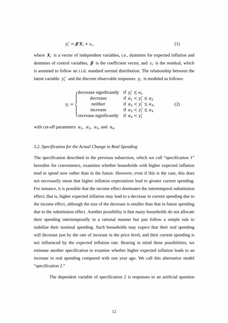
′ , (1)

where is a vector of independent variables, i.e., dummies for expected inflation and

dummies of control variables, is the coefficient vector, and is the residual, which

is assumed to follow an i.i.d. standard normal distribution. The relationship between the

latent variable and the discrete observable responses is modeled as follows:

decrease significantly if decrease if neither if increase if

increase significantly if

, (2)

with cut-off parameters , , , and .

3.2. Specification for the Actual Change in Real Spending

The specification described in the previous subsection, which we call “specification 1”

hereafter for convenience, examines whether households with higher expected inflation

tend to spend now rather than in the future. However, even if this is the case, this does

not necessarily mean that higher inflation expectations lead to greater current spending.

For instance, it is possible that the income effect dominates the intertemporal substitution

effect; that is, higher expected inflation may lead to a decrease in current spending due to

the income effect, although the size of the decrease is smaller than that in future spending

due to the substitution effect. Another possibility is that many households do not allocate

their spending intertemporally in a rational manner but just follow a simple rule to

stabilize their nominal spending. Such households may expect that their real spending

will decrease just by the rate of increase in the price level, and their current spending is

not influenced by the expected inflation rate. Bearing in mind these possibilities, we

estimate another specification to examine whether higher expected inflation leads to an

increase in real spending compared with one year ago. We call this alternative model

“specification 2.”

The dependent variable of specification 2 is responses to an artificial question

12

about the actual change in real spending relative to the previous year. The responses are

constructed employing the same methodology as that used to construct responses about

the expected change in real spending for specification 1, i.e., by synthesizing the

responses to the questions about the actual changes in nominal spending (Q9) and price

levels (Q12) compared with one year ago. The main independent variables are the

dummies for inflation expectations. Although the main independent variables are

identical to those of specification 1, the expected signs on the coefficients in specification

2 are the opposite of those in specification 1. The reason is that if higher expected

inflation leads to a higher level of current spending, this is likely to lower the expected

change in real spending and to raise the actual change compared with one year ago. All

controls used in specification 1 are employed in specification 2 as well. Moreover, since

the dependent variable in specification 2 is the responses about the actual change in

spending, we add dummies corresponding to the actual changes in prices (Q12),

economic conditions (Q1), and real income (constructed using Q7 and Q12) as controls.

These controls for actual changes may be essential. For instance, higher actual inflation

may be associated with lower actual spending growth from one year ago, in part because

households should have increased spending one year ago if they expected such inflation

in advance. At the same time, the actual and expected inflation rates are typically

positively correlated. Thus, unless we control for actual inflation, the coefficient on

expected inflation may be biased, reflecting the effect of actual inflation on actual

spending growth.

4. Baseline Results

This section presents the results from the two baseline specifications described in the

previous section. Table 1 reports the estimated coefficients except those for the dummies

for individuals’ attributes and the time dummies. The table shows that for both

specifications 1 and 2, all four coefficients on expected inflation have the expected signs

and are significant at the 1 percent level. That is, respondents who expect higher inflation

are more likely to indicate that their household will decrease real spending, and to answer

that their household has increased real spending compared with one year ago. These

13

results suggest that higher inflation expectations lead to greater current household

spending.

To gain a quantitative sense of the effects of expected inflation, we define an

aggregate latent variable of the expected change in real spending, which is calculated as

the mean of the latent variables in each wave of the survey:

, (3)

where denotes that the expectation is taken over observations obtained in the survey

at time , rather than over time. Substituting equation (1) into (3) yields

′ , (4)

where is the vector of the means of the independent variables. To derive (4),

we make use of 0, which holds since the residual is independent. We estimate

the aggregate latent variable by using the estimated coefficients for and the

proportion of respondents who chose each choice at time for in equation (4).

Using equation (4), Figure 1 shows a decomposition of the demeaned aggregate

latent variable of specification 1 into the contributions of several groups of dummies.

This decomposition suggests that the contribution of “prices,” which is the sum of the

contributions of four dummies regarding inflation expectations, is quite large. The figure

shows that expected inflation played an important role particularly in 2008 in suppressing

expected real spending growth, which implies that high expected inflation led households

to increase spending. On the other hand, although not reported here, we find that the

contribution of expected inflation in specification 2 is small. This is consistent with Table

1, which shows that the coefficients for specification 2 are much smaller in absolute

value than the corresponding coefficients for specification 1. We will discuss the reasons

behind this large difference between the baseline specifications in the next section.

5. Potential Sources of Estimation Bias and Their Implications

The previous section presented baseline results which suggest that higher inflation

14

expectations lead to greater current household spending. That is, all estimated

coefficients regarding expected inflation have the expected signs and are statistically

significant in both specifications 1 and 2. However, the sizes of the coefficients differ

markedly between these specifications: the coefficients in specification 2 are much

smaller in absolute value than their counterparts in specification 1.

A possible reason for this difference is effects other than the intertemporal

substitution effect: specification 1 is designed to estimate only the substitution effect but

not adverse effects such as the income effect. Thus, by construction, specification 1 is

likely to overestimate the total impact of expected inflation on current spending. In

addition, specification 1 may suffer from the following three possible sources of

estimation bias, although the direction of the bias is not necessarily upward in all cases.

The first potential source of bias is the wording regarding the forecasting

horizon of spending. Note that Q11 asks about the spending plan within the next twelve

months, while Q14 asks about the outlook for prices one year from now. Although most

survey participants may not care about this difference in the wording, it might generate

some bias in our construction of the real spending variables that synthesize these two

questions. In addition, some respondents who anticipate an increase in prices one year

later may expect that their household will rush to increase spending in the near future,

say one month ahead, before prices will go up, although they will decrease spending one

year later. Such respondents may answer that their household will increase spending, and

thus the correlation between expected inflation and the expected change in real spending

may be estimated to be positive. Therefore, to the extent that such respondents play a role,

the difference in the wording may contribute to underestimating the negative relationship

between expected inflation and the expected change in spending growth.

The second potential source of estimation bias is measurement error of expected

inflation. Since we use Q14, the question about expected inflation, to construct the

artificial question about real spending growth, but also use the dummies regarding Q14

as the main independent variables, the estimated coefficients on these dummies may be

biased. To illustrate this possibility, let us use a simple example with quantitative data.

Suppose we have cross-sectional data of the expected inflation rate and the expected

15

nominal spending growth rate . However, these are observed with measurement errors

and , respectively:

, (5)

. (6)

The errors are assumed to be uncorrelated with each other and with the true expectations

and . Suppose also that we compute the observed expected real spending growth

rate as , and regress it on . Then, the least squares estimate of the slope

coefficient is obtained as:

C ,

V

C , V

V V. (7)

Equation (7) suggests that if the variance of the measurement error of expected inflation

Var is large, the estimate of the slope coefficient is biased from its true value of

Cov , / Var . For typical regressions, measurement error works to bias the

estimated coefficients toward zero. However, if the independent variable is used to

construct the dependent variable as here, we cannot tell the direction of the bias. This

type of bias may arise even in our ordered probit models.

The third potential source of bias is our use of grading points to construct the

responses about the expected change in real spending. For instance, we assume that the

absolute value of the grading point is 1 when respondents expect that nominal spending

will increase or decrease, but assign this value only when respondents expect that the

price will go up or down significantly. This assumption may lead to undervaluation of the

effects of expected inflation on expected real spending growth. Another possibility is that

the spending and price level expectations of many respondents may be inconsistent. For

example, survey respondents who expect inflation may not take account of the rise in the

price level when they expect nominal spending growth. If this is the case, our

methodology results in overestimation of the negative correlation between expected real

spending growth and expected inflation.

To assess the possible bias arising from the construction of real variables, we

16

compute the diffusion index of the responses to the artificial question about expected real

spending growth based on the shares of respondents for each choice. We then compare

this diffusion index with the actual year-on-year growth rate of real private consumption,

which is published as a component of the quarterly estimate of GDP, as shown in the

left-hand panel of Figure 2. Similarly, we compute the diffusion index for real income

growth and compare it with the actual year-on-year growth rate of real compensation of

employees, as shown in the right-hand panel of the figure. The panels show that the

diffusion indexes are closely related with and lead the actual growth rates, leading us to

conclude that the constructed data appear to be reasonable proxies for the expected

changes in real spending and real income. This suggests that we can ignore the potential

bias arising from the conversion process from nominal variables into real ones, although

other sources of bias such as measurement error remain.

Specification 2 is much less susceptible to these potential sources of estimation

bias, for the following reasons. First, Q9 asks about the actual change in nominal

spending compared with one year ago, which is the exactly same wording as Q12, the

question about the actual change in prices. Thus, specification 2 is free from any

potential bias due to the difference in wording. Second, the dependent variable is

constructed using the question about the actual change in prices, while the main

independent variables are dummies about the expected change in prices. Because of this

difference in the questions regarding prices, specification 2 suffers less from any

potential measurement error of expected inflation if there is little cross-sectional

correlation between measurement errors regarding expected and actual inflation. Third,

this specification uses the responses about actual inflation both to construct the

dependent variable and as independent variables. Thus, even if the dependent variable is

biased by construction due to over- or underestimation of the effect of the actual change

in prices on that in real spending, the estimation bias of the coefficients on expected

inflation should be limited because it is absorbed into the coefficients on actual inflation.

On the other hand, specification 2 is likely to underestimate the impact of

expected inflation on current spending, since it uses the survey responses about actual

spending growth rather than those about current spending as the dependent variable. If

17

expected inflation from now to one year ahead rises unexpectedly now, both the level of

current spending and the actual spending growth rate should increase. However, if higher

inflation from now to one year ahead was already expected one year ago, current

spending may still be greater but the actual growth rate from one year ago to now is not

necessarily higher, since past spending also may have been greater. Because of this

possibility, the impact of expected inflation on spending growth should be smaller than

that on current spending.

In sum, partly because there are several potential sources of estimation bias, it is

difficult to precisely pin down the magnitude of the impact of expected inflation on

current consumer spending from our results. However, the discussion above suggests that

the positive correlation between expected inflation and actual spending growth is likely

to be underestimated rather than overestimated in specification 2. Therefore, given that in

specification 2 all estimated coefficients regarding expected inflation have the expected

signs and are statistically significant, we can safely conclude that higher expected

inflation leads to greater current consumer spending. Specification 1 does not reflect

adverse effects such as the income effect, and there are several potential sources of bias

in different directions. However, the relatively large estimated coefficients and the

considerable contribution of expected inflation to the aggregate latent variable of the

expected change in real spending shown in Figure 1 suggest that there is a good chance

that the impact of expected inflation is much larger than suggested by the estimated

coefficients in specification 2.

6. Robustness Checks

This section conducts a variety of robustness checks. The first three subsections change

the dependent variable or independent variables. Subsection 6.1 uses nominal spending

instead of real spending as the independent variable to examine whether our method of

constructing the real spending data affects the baseline results. Subsection 6.2 uses

dummies for expected inflation over the next five years (Q16) as independent variables,

while Subsection 6.3 uses quantitative measures of inflation expectations instead of the

18

qualitative ones as main independent variables. Subsections 6.1 and 6.2 check only the

robustness of specification 2, since this specification is more flexible than specification 1,

as will be discussed in detail later. Further, two more subsections, Subsections 6.4 and

6.5, conduct subsample analyses to examine whether the results of specifications 1 and 2

remain unchanged even in subsamples. Specifically, Subsection 6.4 uses subsamples of

each wave of the survey, while Subsection 6.5 uses subsamples by individuals’ attributes.

6.1. Nominal Spending

As argued in Section 5, the results of specification 2 appear to be not susceptible to the

way the artificial variable of real spending is constructed, since this specification uses the

responses about actual inflation both to construct the artificial variable and to control for

various sources of estimation bias. This subsection confirms this argument by using

another specification. We use the survey responses about the actual change in nominal

spending (Q9), instead of that in real spending, as the dependent variable. This

specification does not use the constructed real spending data, and can be utilized to

examine whether our definition of real spending leads to biased estimates. Since the

question about the actual nominal spending growth has three choices (“increased,”

“neither,” and “decreased”), we use an ordered probit model with two thresholds. Table 2

reports the coefficient estimates for expected inflation. The table shows that all the

coefficients on expected inflation have the expected signs and are statistically

significant.7

Note that if we used the responses about expected nominal spending growth as

the dependent variable and found that higher expected inflation leads to a higher

expected change in nominal spending, we could not tell whether higher expected

inflation leads to a higher expected change in real spending or to an increase only in

nominal terms. On the other hand, if the responses about actual nominal spending growth 7 A potential concern is that this specification uses the responses to the artificial questions about the expected and actual changes in real income as controls. We therefore estimated another specification that excludes all dummies for real income. We find that even with this specification, all coefficients on expected inflation have the expected signs and are statistically significant. Although the coefficients are smaller than those for the specification using real income data reported in Table 2, this may reflect potential estimation bias due to the omission of the control variables.

19

are the dependent variable, we can identify the effects of expected inflation, since the

dependent variable and the main independent variables are for different time periods.

6.2. Five-year Inflation Expectations

The main independent variables of the baseline specifications are the dummies for the

expected change in prices one year later. This choice of the forecasting horizon is

essential for specification 1, since this specification is designed to be consistent with the

Euler equation in standard theoretical models, which predict that the expected change in

real spending is positively correlated with the real interest rate of the same horizon. On

the other hand, specification 2 is relatively ad hoc and not strictly linked to structural

relationships. Nevertheless, we used one-year expected inflation even for specification 2,

since survey respondents appear to provide more precise answers with regard to one-year

expected inflation than five-year expected inflation. In addition, shorter-term expected

inflation is more relevant than longer-term expected inflation as a determinant of

spending on less durable goods and services. However, real spending may be associated

not only with shorter-term but also with longer-term expected inflation, in particular with

regard to durables. The reason is that consumers can wait longer for a decrease in prices

if expenditure items are more durable. Thus, this subsection uses data for five-year

expected inflation (Q16) as the main independent variables to check the robustness of

specification 2.

Table 3 presents the estimated coefficients on expected inflation. The column

denoted “5Y only” reports the results for the specification including five-year inflation

expectations only, i.e., excluding one-year expectations, and shows that all four

coefficients on five-year expectations have the expected signs, and three of them are

significant at the 1 percent significance level. The estimated coefficients are generally

smaller than those for one-year expected inflation in specification 2 reported in Table 1

though. Next, the column labeled “1Y and 5Y” reports the results when including both

one- and five-year inflation expectations. All four coefficients on five-year expected

inflation have the expected signs and two of them are still significant at the conventional

5 percent level. However, all four coefficients on one-year expected inflation have the

20

expected signs and are significant. In addition, the coefficients for one-year expectations

are generally larger than those for five-year expectations. These results suggest that our

results for specification 2 are robust to changes in the forecasting horizon of expected

inflation, and that consumer spending is more strongly related with one-year than

five-year expected inflation. The latter result may suggest that respondents with higher

inflation expectations are more likely to assume that the monetary policy authority will

maintain a low policy interest rate within one year but may raise the policy rate within

five years. Another possible reason is that one-year inflation expectations are more

important in determining consumer spending or suffer less from measurement error.

6.3. Quantitative Measures of Expected Inflation

The Opinion Survey asks not only qualitative questions but also quantitative questions

about one- and five-year expected inflation as well as one-year actual inflation (Q15,

Q17, and Q13). We did not use such quantitative data in the baseline specifications, since

Kamada (2008) finds that the quantitative responses about inflation expectations in the

Opinion Survey are biased: there are too many integers, too many zeros, too many

multiples of five, and too few negative numbers. However, we can be more confident

about our baseline results if we obtain similar results even when using such quantitative

measures. Specifically, we use the quantitative measures of expected and actual inflation

as the main independent variables and controls, respectively. As in the previous

subsection, we use five-year expected inflation only for specification 2. Thus, as a

robustness check of specification 1, we use only the quantitative measure of one-year

expected inflation. To check the robustness of specification 2 to changes in the

quantitative measures of inflation expectations, we estimate specifications with one-year

expected inflation only, with five-year expected inflation only, and with both one- and

five-year expectations. For specification 1, we expect the sign on the coefficient to be

negative, while for specification 2, we expect it to be positive. In addition to using the

full sample, in order to avoid potential bias due to outliers, we also use a subsample

excluding respondents who answered that the actual or expected inflation rate is more

than 20 percent or less than minus 20 percent.

21

As can be seen in Table 4, all ten coefficients on expected inflation have the

expected signs. When the responses about expected real spending growth are used as the

dependent variable, as in specification 2, the coefficient is larger when outliers are

excluded. This implies that the outliers make it difficult to detect the relationship

between expected inflation and expected real spending growth. When the responses

about actual spending growth are used, as in specification 2, the coefficient on one-year

expected inflation is significant in all specifications. On the other hand, the estimated

coefficient on five-year expected inflation tends to be small and insignificant, particularly

when both one-year and five-year expectations are included. This is consistent with the

results of the previous subsection, and confirms that consumer spending is more strongly

related with one-year than with five-year inflation expectations.

6.4. Subsample Analysis by Survey Wave

This subsection investigates whether our results for specifications 1 and 2 are robust to

using subsamples for each survey wave.8 Figures 3 and 4 display the coefficient

estimates for four dummies regarding expected inflation for each survey wave, together

with the 95 percent confidence intervals. These figures show that the estimated

coefficients are rather stable over time. That is, the point estimates of specification 1

shown in Figure 3 have the expected signs for all four dummies and all periods, although

they are insignificant for some dummies and periods. Figure 4 shows that the coefficients

from specification 2 have the expected signs when they are significantly different from

zero. These results are consistent with the baseline full-sample results.

The policy interest rate of the Bank of Japan was higher than the current level of

effectively zero and reached 0.5 percent in the earlier part of our observation period.

However, there is no clear difference in the coefficient estimates between earlier and later

observations, as shown in Figures 3 and 4. This supports our view that a policy interest

rate of 0.5 percent is essentially equivalent to zero for households. The stable coefficient

estimates also imply that the estimated relationship between expected inflation and

8 We of course exclude time dummies when estimating the specifications for subsamples of each survey wave.

22

spending can be interpreted as a structural relationship rather than a statistical artifact

that is relevant only for particular situations. That is, the relationship appears to be very

stable despite the numerous events that occurred during the observation period, such as

the global financial crisis, the introduction of various unconventional monetary policies,

and the adoption of government policies such as subsidies for environmentally friendly

vehicles. If the baseline results were an artifact of our reduced-form specifications, we

would expect the estimated coefficients to show greater fluctuations in response to such

events.

6.5. Subsample Analysis by Individuals’ Attributes

As a further check, we explore whether our main findings differ across respondents with

different attributes. We focus on the differences in asset holdings, financial literacy, and

age, which the literature refers to as potential factors influencing the relationship between

real interest rates and saving-consumption decisions. As highlighted by Zeldes (1989),

asset holders are less likely to be liquidity constrained and can therefore more easily

choose the timing of their spending. Thus, the intertemporal substitution effect may be

stronger for them than for others. Age also may influence the relationship between

expected inflation and real spending. For instance, older people are more likely to vividly

remember the high inflation episodes in the 1970s, and thus their spending may be more

sensitive to expected inflation. Financial literacy as well may be important for rational

intertemporal spending decisions.

For our analysis, we define asset holders as those who, for example in the

question about the reasons behind the increased spending (Q9-(a)), responded “because

the value of my household’s financial assets such as stocks and bonds has increased.”9

9 Specifically, asset holders are defined as those who, in the questions about the reasons why household circumstances have become better (worse) (Q6-(a) and Q6-(b)), responded “because my interest income and dividend payments have increased (decreased)” or “because the value of my household’s assets such as real estate and stocks has increased (declined),” or those who, in the question about the reasons behind the increased (decreased) spending (Q9-(a) and Q9-(b)), responded “because the value of my household’s non-financial assets such as real estate has increased (decreased)” or “because the value of my household’s financial assets such as stocks and bonds has increased (decreased).”

23

Individuals with high financial literacy are defined as those who, in the question about

the reasons behind their assessment of economic conditions (Q2), answered “economic

indicators and statistics.” Finally, we roughly split the sample in half by age group: the

young (aged 20-49) and the old (age 50 and over). We estimate both specifications 1 and

2 for each of the following six subsamples: those with assets, those without assets, the

old, the young, those with high financial literacy, and those with low financial literacy.

Table 5 reports the estimated coefficients on expected inflation. The table shows

that our main findings are robust across all six subsamples: all 48 coefficients have the

expected signs, and many of them are significant at the 5 percent level. For asset holders

and older respondents, the coefficients tend to be relatively large in absolute value. This

suggests that within these categories expected inflation is rather important in determining

differences in spending attitudes. However, these results do not necessarily imply that the

importance of expected inflation differs across different categories. The coefficients are

not directly comparable across subsamples, since the subsample analysis examines the

determinants of relative spending attitudes within each category rather than across

categories. Nevertheless, as shown in the next section, we obtain similar results when

analyzing differences in the relative importance of determinants of spending across

categories.

7. The Effects of Individuals’ Attributes

As discussed in Subsection 6.5, subsample analysis is not necessarily useful to compare

the effects of individuals’ attributes across groups. To examine the effects on the

relationship between expected inflation and spending attitudes, this section adds

interaction terms into the ordered probit models as independent variables. The attributes

of individuals that we focus on are the same as those in Subsection 6.5, namely, whether

individuals hold assets, their financial literacy, and age. We check the effects for three

specifications used so far: specifications 1 and 2, and the specification with actual

nominal spending growth employed in Subsection 6.1. The latter specification, which we

call “specification 3,” is used because of the concern that our construction of real

24

spending growth may lead to substantial estimation bias. As for the effects of holding

assets, for instance, we use a dummy for asset holders that takes unity for asset holders

and zero otherwise. We then add this dummy and interaction terms between this dummy

and all independent variables to each of the three specifications. Similarly, dummies for

high financial literacy and older respondents are used. In total, nine specifications, which

are constructed by combining the three base specifications with different dependent

variables (specifications 1, 2, and 3) and three dummies for individuals’ attributes, are

estimated. We focus on the estimated coefficients on the interaction terms regarding

expected inflation. For a given attribute, the more interaction terms have the expected

signs, which are the same as the expected signs on the coefficients regarding expected

inflation, the stronger is the positive relationship between current spending and inflation

expectations for individuals with that attribute. We also conduct the Wald test with the

null hypothesis that all four coefficients on the interaction terms regarding expected

inflation are zero.

Table 6 shows that the interaction terms tend to have the expected signs in the

case of asset holders and older respondents, but there is no clear pattern in the case of

people with high financial literacy. In particular, all four coefficients have the expected

signs for asset holders for specification 3 and for older respondents for specifications 2

and 3. Table 7 reports the p-values of the Wald test and shows that the null hypothesis is

rejected at the 5 percent level for two of the three cases where all four coefficients have

the expected signs, while the Wald test just marginally fails to reject the null at the 10

percent level for the other case. These results imply that the effects of expected inflation

on household spending are relatively stronger for asset holders and older respondents.

These findings may reflect that asset holders are less likely to be liquidity constrained,

while older people are more likely to remember the high inflation episodes in the 1970s,

so that their spending may be more sensitive to expected inflation and the intertemporal

substitution effect is stronger for them. However, these interpretations are rather tentative,

since there is no clear tendency that the coefficients have the expected signs in

specification 1, which, unlike specifications 2 and 3, is designed to focus on the

intertemporal substitution effect. On the other hand, we should also keep the possibility

in mind that the results of specification 1 may suffer from estimation bias, as discussed in

25

Section 5.

As discussed by Ichiue and Shimizu (2012), at least in Japan older people on

average tend to hold more assets. This is a possible reason for our finding that both asset

holding and age have an effect on the relationship between inflation expectations and

spending. To examine this possibility, we add dummies for asset holders and older people

as well as interaction terms between the two dummies and the independent variables

simultaneously to each of the base specifications. Table 8 presents the results and shows

that the signs of most of the coefficients are the same as in Table 6. This suggests that

holding assets and age independently affect the relationship between expected inflation

and household spending.

8. Conclusion

This paper uses micro data for Japan, which has experienced extremely low interest rates

for a prolonged period, to examine the relationship between expected inflation and

household spending. The empirical results suggest that higher inflation expectations tend

to result in greater current household spending at the ZLB. While it is difficult to pin

down the quantitative impact of expected inflation on spending, our results are fairly

robust to a variety of specifications.

The results of our analysis stand in stark contrast with those of Bachmann et al.

(2013), who, using micro data for the United States, find that the relationship between

expected inflation and spending is small and often insignificant. There are several

possible reasons for the difference in the results. For instance, the difference in the

coverage of expenditure items between expected inflation and spending attitudes in the

US data may make it difficult to detect the relationship between them. Another potential

reason is that, at least until 2010, the end of the sample used by Bachmann et al. (2013),

US households may not have understood the new regime where the central bank does not

raise the nominal policy interest rate even if inflation rises.

Although our analysis provides some evidence in support of the notion that

higher expected inflation leads to greater current consumer spending, this result alone

26

does not immediately justify the proposition that central banks should commit to high

inflation at the ZLB. For instance, if it takes time for people to understand a new regime

of a fixed nominal interest rate, committing to higher inflation may not be effective

during the early stages of a ZLB environment.

An important task for the future is to identify the reasons behind the difference

between Bachmann et al.’s (2013) results and ours. For instance, the Preference

Parameters Study conducted by Osaka University since 2003 has collected panel survey

data on household behavior and expectations including quantitative measures of both

inflation and spending for four countries, including both Japan and the United States.

Although these data are collected only on an annual basis, using them for analysis may

be helpful for understanding the reasons behind the different empirical results obtained

so far.

27

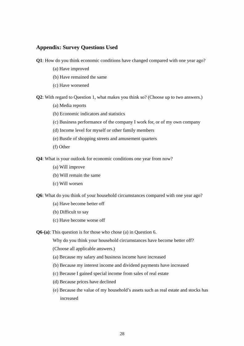
Appendix: Survey Questions Used

Q1: How do you think economic conditions have changed compared with one year ago?

(a) Have improved

(b) Have remained the same

(c) Have worsened

Q2: With regard to Question 1, what makes you think so? (Choose up to two answers.)

(a) Media reports

(b) Economic indicators and statistics

(c) Business performance of the company I work for, or of my own company

(d) Income level for myself or other family members

(e) Bustle of shopping streets and amusement quarters

(f) Other

Q4: What is your outlook for economic conditions one year from now?

(a) Will improve

(b) Will remain the same

(c) Will worsen

Q6: What do you think of your household circumstances compared with one year ago?

(a) Have become better off

(b) Difficult to say

(c) Have become worse off

Q6-(a): This question is for those who chose (a) in Question 6.

Why do you think your household circumstances have become better off?

(Choose all applicable answers.)

(a) Because my salary and business income have increased

(b) Because my interest income and dividend payments have increased

(c) Because I gained special income from sales of real estate

(d) Because prices have declined

(e) Because the value of my household’s assets such as real estate and stocks has

increased

28

(f) Because the number of dependents in my household has decreased

(g) Other

Q6-(b): This question is for those who chose (c) in Question 6.

Why do you think your household circumstances have become worse off?

(Choose all applicable answers.)

(a) Because my salary and business income have decreased

(b) Because my interest income and dividend payments have decreased

(c) Because I purchased real estate

(d) Because prices have risen

(e) Because the value of my household’s assets such as real estate and stocks has

declined

(f) Because the number of dependents in my household has increased

(g) Other

Q7: How has your household income changed compared with one year ago?

(a) Has increased

(b) Has remained the same

(c) Has decreased

Q8: What is your outlook for household income one year from now?

(a) Will increase

(b) Will remain the same

(c) Will decrease

Q9: How has your household changed its spending compared with one year ago?

(a) Has increased

(b) Has neither increased nor decreased

(c) Has decreased

Q9-(a): This question is for those who chose (a) in Question 9.

Why has your household increased its spending? (Choose all applicable answers.)

(a) Because my income has increased

(b) Because my income is likely to increase in the future

29

(c) Because the value of my household’s non-financial assets such as real estate

has increased

(d) Because the value of my household’s financial assets such as stocks and

bonds has increased

(e) Because I purchased real estate such as a house

(f) Because I purchased consumer durable goods such as a car

(g) Because my spending has risen due to an increased number of dependents in

my household

(h) Because the costs of consumer goods and services have risen

(i) Other

Q9-(b): This question is for those who chose (c) in Question 9.

Why has your household decreased its spending? (Choose all applicable answers.)

(a) Because my income has decreased

(b) Because my income is not likely to increase in the future

(c) Because the value of my household’s non-financial assets such as real estate

has decreased

(d) Because the value of my household’s financial assets such as stocks and

bonds has decreased

(e) Because my spending has fallen due to a decreased number of dependents in

my household

(f) Other

Q11: How does your household plan to change its spending within the next twelve

months?

(a) Will increase

(b) Will neither increase nor decrease

(c) Will decrease

Q12: How do you think prices have changed compared with one year ago?

(a) Have gone up significantly

(b) Have gone up slightly

(c) Have remained almost unchanged

30

(d) Have gone down slightly

(e) Have gone down significantly

Q13: By what percent do you think prices have changed compared with one year ago?

Please choose “up” or “down” and fill in the box below with a specific figure. If

you think that they have been unchanged, please put a “0.”

Prices have gone up/down about percent compared with one year ago.

Q14: What is your outlook for prices one year from now?






Q15: By what percent do you think prices will change one year from now?

Please choose “up” or “down” and fill in the box below with a specific figure. If

you think that they will be unchanged, please put a “0.”

Prices will go up/down about percent one year from now.

Q16: What is your outlook for prices over the next five years?






Q17: By what percent do you think prices will change per year on average over the next

five years? Please choose “up” or “down” and fill in the box below with a specific

figure. If you think that they will be unchanged, please put a “0.”

Prices will go up/down about percent per year on average over the next

five years.

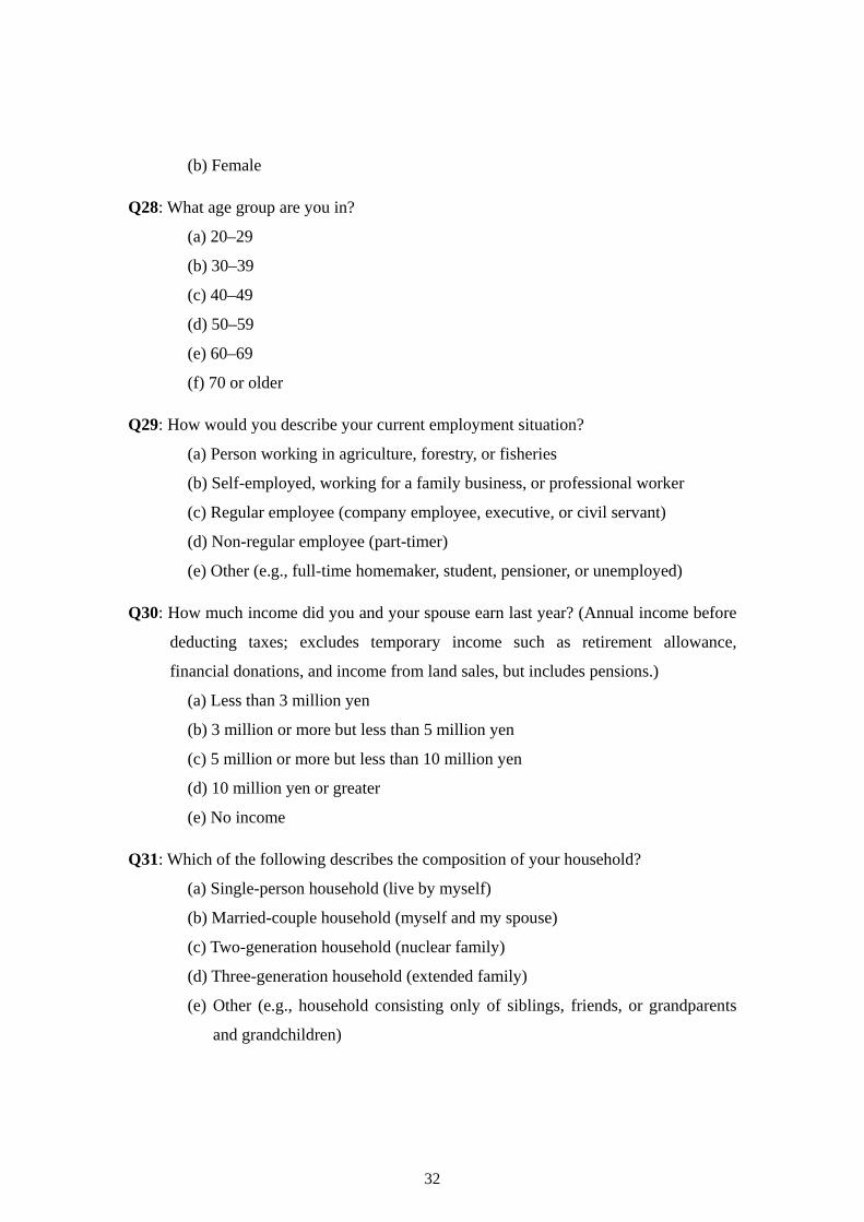
Q27: Are you male or female?

(a) Male

31

(b) Female

Q28: What age group are you in?

(a) 20–29

(b) 30–39

(c) 40–49

(d) 50–59

(e) 60–69

(f) 70 or older

Q29: How would you describe your current employment situation?

(a) Person working in agriculture, forestry, or fisheries

(b) Self-employed, working for a family business, or professional worker

(c) Regular employee (company employee, executive, or civil servant)

(d) Non-regular employee (part-timer)

(e) Other (e.g., full-time homemaker, student, pensioner, or unemployed)

Q30: How much income did you and your spouse earn last year? (Annual income before

deducting taxes; excludes temporary income such as retirement allowance,

financial donations, and income from land sales, but includes pensions.)

(a) Less than 3 million yen

(b) 3 million or more but less than 5 million yen

(c) 5 million or more but less than 10 million yen

(d) 10 million yen or greater

(e) No income

Q31: Which of the following describes the composition of your household?

(a) Single-person household (live by myself)

(b) Married-couple household (myself and my spouse)

(c) Two-generation household (nuclear family)

(d) Three-generation household (extended family)

(e) Other (e.g., household consisting only of siblings, friends, or grandparents

and grandchildren)

32

References

Attanasio, O. P. and G. Weber (1993), “Consumption Growth, the Interest Rate and Aggregation,” Review of Economic Studies 60, 631-649.

Baba, N. (2000), “Exploring the Role of Money in Asset Pricing in Japan: Monetary Considerations and Stochastic Discount Factors,” Monetary and Economic Studies 18(1), 159-198.

Bachmann, R., T. O. Berg and E. R. Sims (2013), “Inflation Expectations and Readiness to Spend: Cross-Sectional Evidence,” http://www.vwlmac.rwth-aachen.de/ team/bachmann/ An earlier version of this paper is circulated as NBER Working Paper 17958.

Christiano, L. J., M. Eichenbaum and C. L. Evans (2005), “Nominal Rigidities and the Dynamic Effects of a Shock to Monetary Policy,” Journal of Political Economy 113, 1-45.

Delong, J. B. and L. H. Summers (2012), “Fiscal Policy in a Depressed Economy,” Brookings Papers on Economic Activity 1:2012, 233-297.

Eggertsson, G. B. and M. Woodford (2003), “The Zero Bound on Interest Rates and Optimal Monetary Policy,” Brookings Papers on Economic Activity 1:2003, 139-211.

Hamori, S. (1992), “Test of C-CAPM for Japan: 1980-1988,” Economics Letters 38, 67-72.

Hamori, S. (1996), “Consumption Growth and the Intertemporal Elasticity of Substitution: Some Evidence from Income Quintile Groups in Japan,” Applied Economics Letters 3, 529-532.

Hayashi, F. (1985), “The Permanent Income Hypothesis and Consumption Durability: Analysis Based on Japanese Panel Data,” Quarterly Journal of Economics 100, 1083-1113.

Ichiue, H. and Y. Shimizu (2012), “Determinants of Long-term Yields: A Panel Data Analysis of Major Countries and Decomposition of Yields of Japan and the US,” Bank of Japan Working Paper Series 12-E-7.

Kamada, K. (2008), “Kakei no Bukka Mitoshi no Kahou Kouchokusei: ‘Seikatsu Ishiki ni Kansuru Anketo Chosa’ wo Mochiita Bunseki (Downward Rigidity of Households’ Expected Inflation: An Analysis Using the Opinion Survey on the General Public’s Views and Behavior),” Bank of Japan Working Paper Series 08-J-8 (in Japanese).

Kitamura, Y. and H. Fujiki (1997), “Sapurai Saido Jouhou wo Riyou Shita Shouhi ni

33

Motozuku Shisan Kakaku Moderu no Suikei (Estimation of the Consumption-Based Capital Asset Pricing Model Using Information on the Supply Side),” Kinyu Kenkyu 16(4), 137-154 (in Japanese).

Krugman, P. R. (1998), “It's Baaack: Japan’s Slump and the Return of the Liquidity Trap,” Brookings Papers on Economic Activity 2:1998, 137-205.

Nakano, K. and M. Saito (1998), “Asset Pricing in Japan,” Journal of the Japanese and International Economies 12, 151-166.

Romer, C. (2011), “Dear Ben: It’s Time for Your Volcker Moment,” The New York Times, October 29, 2011.

Taylor, J. B. (1993), “Discretion versus Policy Rules in Practice,” Carnegie-Rochester Conference Series on Public Policy 39, 195-214.

Wieland, J. (2012), “Are Negative Supply Shocks Expansionary at the Zero Lower Bound? Inflation Expectations and Financial Frictions in Sticky-Price Models,” mimeo.

Woodford, M. (2012), “Methods of Policy Accommodation at the Interest-Rate Lower Bound,” Presented at “The Changing Policy Landscape,” 2012 FRB Kansas City Economic Policy Symposium, Jackson Hole, WY, USA.

Zeldes, S. P. (1989), “Consumption and Liquidity Constraints: An Empirical Investigation,” Journal of Political Economy 97, 305-346.

34

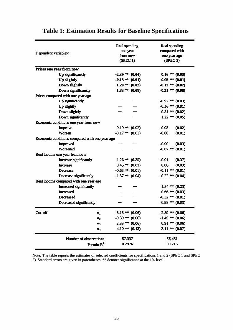
Table 1: Estimation Results for Baseline Specifications

Prices one year from now Up significantly -2.39 ** (0.04) 0.16 ** (0.03)Up slightly -0.13 ** (0.01) 0.05 ** (0.01)Down slightly 1.20 ** (0.02) -0.12 ** (0.02)Down significantly 1.83 ** (0.08) -0.31 ** (0.08)

Prices compared with one year ago Up significantly ― ― -0.92 ** (0.03)Up slightly ― ― -0.56 ** (0.01)Down slightly ― ― 0.31 ** (0.02)Down significantly ― ― 1.22 ** (0.05)

Economic conditions one year from now Improve 0.19 ** (0.02) -0.03 (0.02)Worsen -0.17 ** (0.01) -0.00 (0.01)

Economic conditions compared with one year ago Improved ― ― -0.00 (0.03)Worsened ― ― -0.07 ** (0.01)

Real income one year from now Increase significantly 1.26 ** (0.35) -0.01 (0.37)Increase 0.45 ** (0.03) 0.06 (0.03)Decrease -0.63 ** (0.01) -0.11 ** (0.01)Decrease significantly -1.37 ** (0.04) -0.22 ** (0.04)

Real income compared with one year ago Increased significantly ― ― 1.54 ** (0.23)Increased ― ― 0.66 ** (0.03)Decreased ― ― -0.52 ** (0.01)Decreased significantly ― ― -0.98 ** (0.03)

Cut-off α1 -3.15 ** (0.06) -2.89 ** (0.06)α2 -0.30 ** (0.06) -1.49 ** (0.06)α3 2.33 ** (0.06) 0.91 ** (0.06)α4 4.10 ** (0.13) 3.11 ** (0.07)

Number of observations

Pseudo R2

Real spendingcompared withone year ago

(SPEC 2)

Dependent variables:

57,3370.2976

56,4510.1715

Real spendingone year

from now(SPEC 1)







Cut-off α1 -3.15 ** (0.06) -2.89 ** (0.06)α2 -0.30 ** (0.06) -1.49 ** (0.06)α3 2.33 ** (0.06) 0.91 ** (0.06)α4 4.10 ** (0.13) 3.11 ** (0.07)


Pseudo R2


(SPEC 2)


57,3370.2976

56,4510.1715


from now(SPEC 1)







Cut-off α1 -3.15 ** (0.06) -2.89 ** (0.06)α2 -0.30 ** (0.06) -1.49 ** (0.06)α3 2.33 ** (0.06) 0.91 ** (0.06)α4 4.10 ** (0.13) 3.11 ** (0.07)


Pseudo R2


(SPEC 2)


57,3370.2976

56,4510.1715


from now(SPEC 1)







Cut-off α1 -3.15 ** (0.06) -2.89 ** (0.06)α2 -0.30 ** (0.06) -1.49 ** (0.06)α3 2.33 ** (0.06) 0.91 ** (0.06)α4 4.10 ** (0.13) 3.11 ** (0.07)


Pseudo R2


(SPEC 2)


57,3370.2976

56,4510.1715


from now(SPEC 1)







Cut-off α1 -3.15 ** (0.06) -2.89 ** (0.06)α2 -0.30 ** (0.06) -1.49 ** (0.06)α3 2.33 ** (0.06) 0.91 ** (0.06)α4 4.10 ** (0.13) 3.11 ** (0.07)


Pseudo R2


(SPEC 2)


57,3370.2976

56,4510.1715


from now(SPEC 1)







Cut-off α1 -3.15 ** (0.06) -2.89 ** (0.06)α2 -0.30 ** (0.06) -1.49 ** (0.06)α3 2.33 ** (0.06) 0.91 ** (0.06)α4 4.10 ** (0.13) 3.11 ** (0.07)


Pseudo R2


(SPEC 2)


57,3370.2976

56,4510.1715


from now(SPEC 1)

Note: The table reports the estimates of selected coefficients for specifications 1 and 2 (SPEC 1 and SPEC2). Standard errors are given in parentheses. ** denotes significance at the 1% level.







Cut-off α1 -3.15 ** (0.06) -2.89 ** (0.06)α2 -0.30 ** (0.06) -1.49 ** (0.06)α3 2.33 ** (0.06) 0.91 ** (0.06)α4 4.10 ** (0.13) 3.11 ** (0.07)


Pseudo R2


(SPEC 2)


57,3370.2976

56,4510.1715


from now(SPEC 1)

Note: The table reports the estimates of selected coefficients for specifications 1 and 2 (SPEC 1 and SPEC2). Standard errors are given in parentheses. ** denotes significance at the 1% level.







Cut-off α1 -3.15 ** (0.06) -2.89 ** (0.06)α2 -0.30 ** (0.06) -1.49 ** (0.06)α3 2.33 ** (0.06) 0.91 ** (0.06)α4 4.10 ** (0.13) 3.11 ** (0.07)


Pseudo R2


(SPEC 2)


57,3370.2976

56,4510.1715


from now(SPEC 1)

35

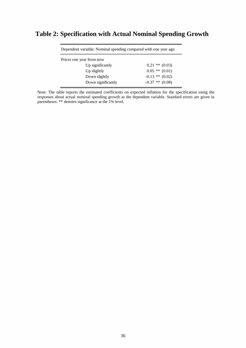
Table 2: Specification with Actual Nominal Spending Growth

Note: The table reports the estimated coefficients on expected inflation for the specification using theresponses about actual nominal spending growth as the dependent variable. Standard errors are given inparentheses. ** denotes significance at the 1% level.

Prices one year from now Up significantly 0.21 ** (0.03)

Up slightly 0.05 ** (0.01)Down slightly -0.13 ** (0.02)

Down significantly -0.37 ** (0.08)

Dependent variable: Nominal spending compared with one year ago

36

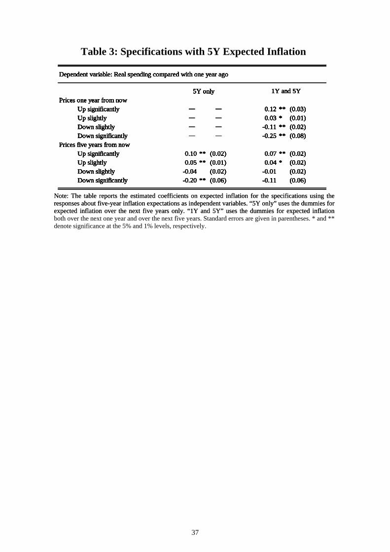
Table 3: Specifications with 5Y Expected Inflation

Dependent variable: Real spending compared with one year ago

5Y onlyPrices one year from now

Up significantly ― ― 0.12 ** (0.03)

Up slightly ― ― 0.03 * (0.01)Down slightly ― ― -0.11 ** (0.02)Down significantly ― ― -0.25 ** (0.08)

Prices five years from now Up significantly 0.10 ** (0.02) 0.07 ** (0.02)Up slightly 0.05 ** (0.01) 0.04 * (0.02)

Down slightly -0.04 (0.02) -0.01 (0.02)Down significantly -0.20 ** (0.06) -0.11 (0.06)

1Y and 5Y







1Y and 5Y

Note: The table reports the estimated coefficients on expected inflation for the specifications using theresponses about five-year inflation expectations as independent variables. “5Y only” uses the dummies forexpected inflation over the next five years only. “1Y and 5Y” uses the dummies for expected inflationb h h d h fi S d d i i h * d **







1Y and 5Y

Note: The table reports the estimated coefficients on expected inflation for the specifications using theresponses about five-year inflation expectations as independent variables. “5Y only” uses the dummies forexpected inflation over the next five years only. “1Y and 5Y” uses the dummies for expected inflationboth over the next one year and over the next five years. Standard errors are given in parentheses. * and **denote significance at the 5% and 1% levels, respectively.







1Y and 5Y







1Y and 5Y







1Y and 5Y







1Y and 5Y







1Y and 5Y

37

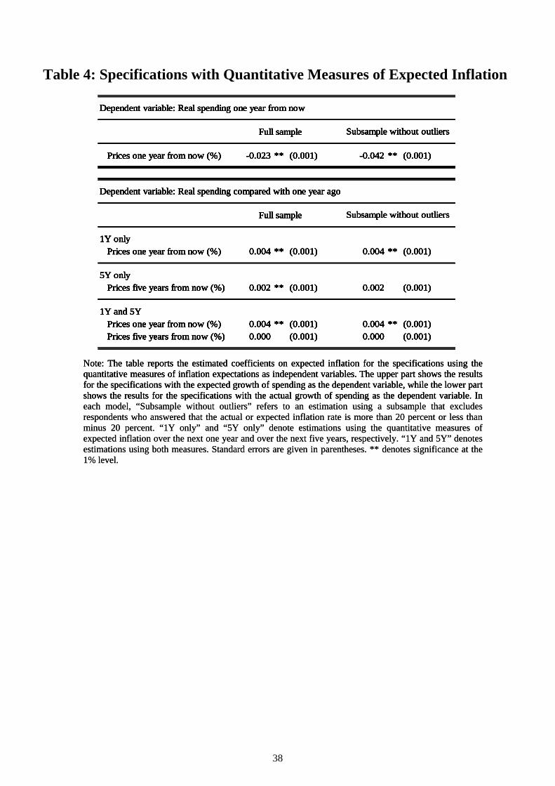
Table 4: Specifications with Quantitative Measures of Expected Inflation

Dependent variable: Real spending one year from now

Full sample

Prices one year from now (%) -0.023 ** (0.001) -0.042 ** (0.001)


Full sample

1Y only Prices one year from now (%) 0.004 ** (0.001) 0.004 ** (0.001)

5Y only Prices five years from now (%) 0.002 ** (0.001) 0.002 (0.001)

1Y and 5Y Prices one year from now (%) 0.004 ** (0.001) 0.004 ** (0.001) Prices five years from now (%) 0.000 (0.001) 0.000 (0.001)

Subsample without outliers



Full sample



Full sample







Full sample



Full sample






Note: The table reports the estimated coefficients on expected inflation for the specifications using thequantitative measures of inflation expectations as independent variables. The upper part shows the resultsfor the specifications with the expected growth of spending as the dependent variable, while the lower partshows the results for the specifications with the actual growth of spending as the dependent variable. In


Full sample



Full sample






Note: The table reports the estimated coefficients on expected inflation for the specifications using thequantitative measures of inflation expectations as independent variables. The upper part shows the resultsfor the specifications with the expected growth of spending as the dependent variable, while the lower partshows the results for the specifications with the actual growth of spending as the dependent variable. Ineach model, “Subsample without outliers” refers to an estimation using a subsample that excludesrespondents who answered that the actual or expected inflation rate is more than 20 percent or less thanminus 20 percent. “1Y only” and “5Y only” denote estimations using the quantitative measures ofexpected inflation over the next one year and over the next five years, respectively. “1Y and 5Y” denotesestimations using both measures. Standard errors are given in parentheses. ** denotes significance at the1% level.


Full sample



Full sample






Note: The table reports the estimated coefficients on expected inflation for the specifications using thequantitative measures of inflation expectations as independent variables. The upper part shows the resultsfor the specifications with the expected growth of spending as the dependent variable, while the lower partshows the results for the specifications with the actual growth of spending as the dependent variable. Ineach model, “Subsample without outliers” refers to an estimation using a subsample that excludesrespondents who answered that the actual or expected inflation rate is more than 20 percent or less thanminus 20 percent. “1Y only” and “5Y only” denote estimations using the quantitative measures ofexpected inflation over the next one year and over the next five years, respectively. “1Y and 5Y” denotesestimations using both measures. Standard errors are given in parentheses. ** denotes significance at the1% level.


Full sample



Full sample






38

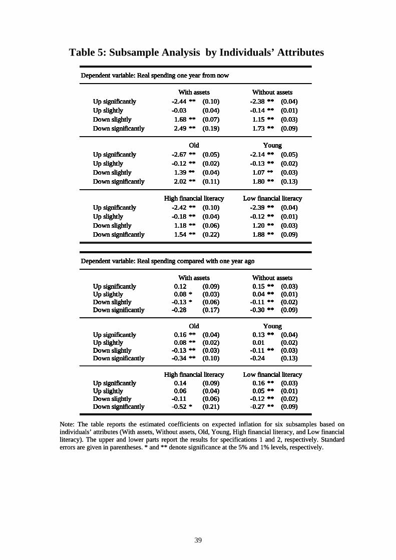
Table 5: Subsample Analysis by Individuals’ Attributes


Up significantly -2.44 ** (0.10) -2.38 ** (0.04)Up slightly -0.03 (0.04) -0.14 ** (0.01)

Down slightly 1.68 ** (0.07) 1.15 ** (0.03)Down significantly 2.49 ** (0.19) 1.73 ** (0.09)

Up significantly -2.67 ** (0.05) -2.14 ** (0.05)Up slightly -0.12 ** (0.02) -0.13 ** (0.02)Down slightly 1.39 ** (0.04) 1.07 ** (0.03)Down significantly 2.02 ** (0.11) 1.80 ** (0.13)



Up significantly 0.12 (0.09) 0.15 ** (0.03)Up slightly 0.08 * (0.03) 0.04 ** (0.01)Down slightly -0.13 * (0.06) -0.11 ** (0.02)Down significantly -0.28 (0.17) -0.30 ** (0.09)

Up significantly 0.16 ** (0.04) 0.13 ** (0.04)Up slightly 0.08 ** (0.02) 0.01 (0.02)Down slightly -0.13 ** (0.03) -0.11 ** (0.03)Down significantly -0.34 ** (0.10) -0.24 (0.13)

Up significantly 0.14 (0.09) 0.16 ** (0.03)Up slightly 0.06 (0.04) 0.05 ** (0.01)Down slightly -0.11 (0.06) -0.12 ** (0.02)Down significantly -0.52 * (0.21) -0.27 ** (0.09)

With assets Without assets

Old Young

High financial literacy Low financial literacy

Old Young













Old Young


Old Young













Old Young


Old Young













Old Young


Old Young













Old Young


Old Young













Old Young


Old Young



Note: The table reports the estimated coefficients on expected inflation for six subsamples based onindividuals’ attributes (With assets, Without assets, Old, Young, High financial literacy, and Low financialliteracy). The upper and lower parts report the results for specifications 1 and 2, respectively. Standarderrors are given in parentheses. * and ** denote significance at the 5% and 1% levels, respectively.











Old Young


Old Young



Note: The table reports the estimated coefficients on expected inflation for six subsamples based onindividuals’ attributes (With assets, Without assets, Old, Young, High financial literacy, and Low financialliteracy). The upper and lower parts report the results for specifications 1 and 2, respectively. Standarderrors are given in parentheses. * and ** denote significance at the 5% and 1% levels, respectively.











Old Young


Old Young



39

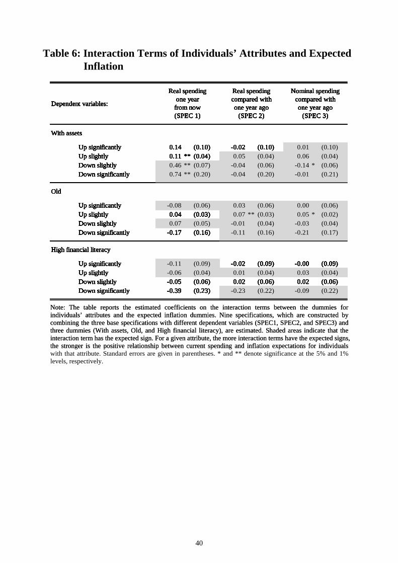
Table 6: Interaction Terms of Individuals’ Attributes and Expected Inflation '


With assets

Up significantly 0.14 (0.10) -0.02 (0.10) 0.01 (0.10)Up slightly 0.11 ** (0.04) 0.05 (0.04) 0.06 (0.04)Down slightly 0.46 ** (0.07) -0.04 (0.06) -0.14 * (0.06)Down significantly 0.74 ** (0.20) -0.04 (0.20) -0.01 (0.21)

Old

Up significantly -0.08 (0.06) 0.03 (0.06) 0.00 (0.06)Up slightly 0.04 (0.03) 0.07 ** (0.03) 0.05 * (0.02)Down slightly 0.07 (0.05) -0.01 (0.04) -0.03 (0.04)Down significantly -0.17 (0.16) -0.11 (0.16) -0.21 (0.17)

High financial literacy

Up significantly -0.11 (0.09) -0.02 (0.09) -0.00 (0.09)Up slightly -0.06 (0.04) 0.01 (0.04) 0.03 (0.04)Down slightly -0.05 (0.06) 0.02 (0.06) 0.02 (0.06)Down significantly -0.39 (0.23) -0.23 (0.22) -0.09 (0.22)


from now(SPEC 1)


(SPEC 2)

Nominal spendingcompared withone year ago

(SPEC 3)


With assets


Old





from now(SPEC 1)


(SPEC 2)


(SPEC 3)


With assets


Old





from now(SPEC 1)


(SPEC 2)


(SPEC 3)


With assets


Old





from now(SPEC 1)


(SPEC 2)


(SPEC 3)

Note: The table reports the estimated coefficients on the interaction terms between the dummies forindividuals’ attributes and the expected inflation dummies. Nine specifications, which are constructed bycombining the three base specifications with different dependent variables (SPEC1, SPEC2, and SPEC3) andthree dummies (With assets, Old, and High financial literacy), are estimated. Shaded areas indicate that theinteraction term has the expected sign. For a given attribute, the more interaction terms have the expected signs,the stronger is the positive relationship between current spending and inflation expectations for individuals


With assets


Old





from now(SPEC 1)


(SPEC 2)


(SPEC 3)

Note: The table reports the estimated coefficients on the interaction terms between the dummies forindividuals’ attributes and the expected inflation dummies. Nine specifications, which are constructed bycombining the three base specifications with different dependent variables (SPEC1, SPEC2, and SPEC3) andthree dummies (With assets, Old, and High financial literacy), are estimated. Shaded areas indicate that theinteraction term has the expected sign. For a given attribute, the more interaction terms have the expected signs,the stronger is the positive relationship between current spending and inflation expectations for individualswith that attribute. Standard errors are given in parentheses. * and ** denote significance at the 5% and 1%levels, respectively.


With assets


Old





from now(SPEC 1)


(SPEC 2)


(SPEC 3)


With assets


Old





from now(SPEC 1)


(SPEC 2)


(SPEC 3)


With assets


Old





from now(SPEC 1)


(SPEC 2)


(SPEC 3)

40

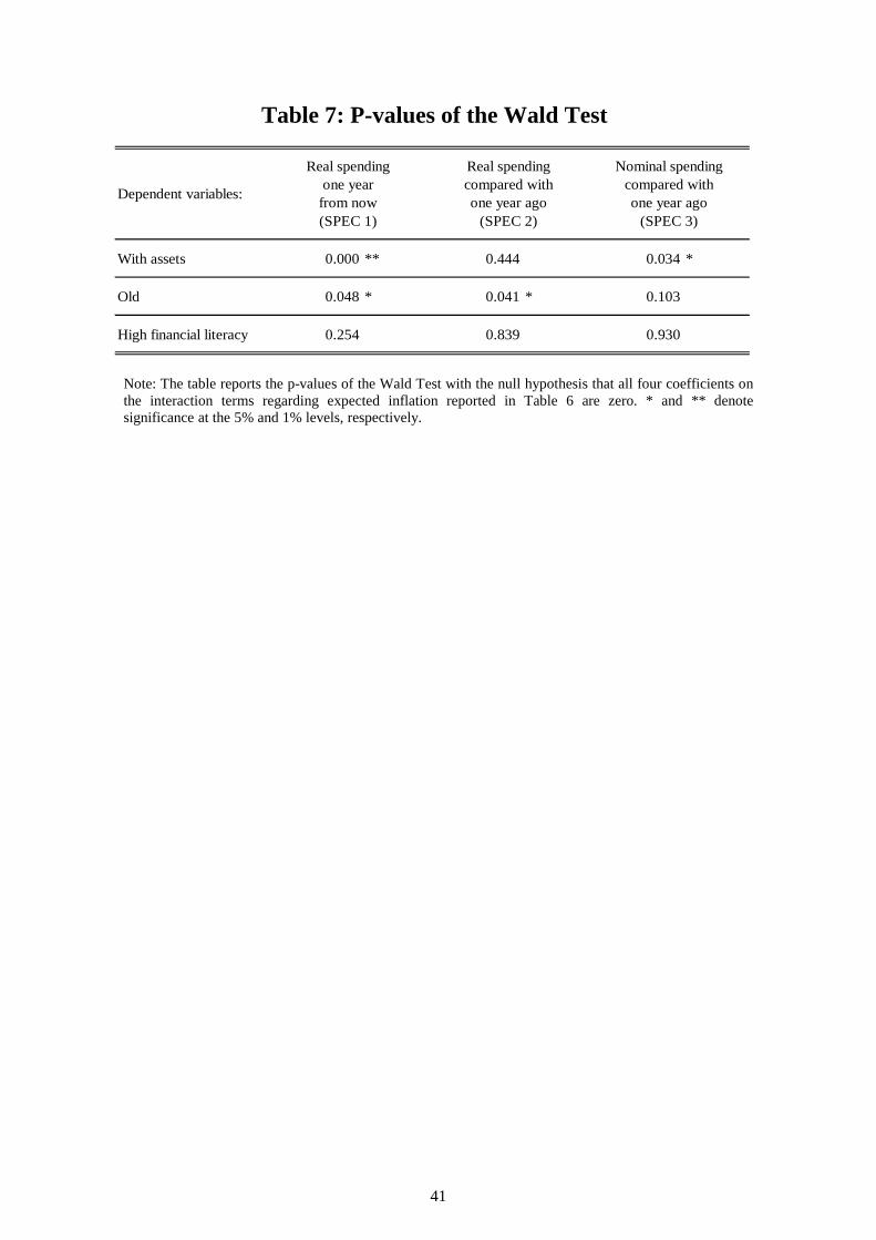
Table 7: P-values of the Wald Test

Note: The table reports the p-values of the Wald Test with the null hypothesis that all four coefficients onthe interaction terms regarding expected inflation reported in Table 6 are zero. * and ** denotesignificance at the 5% and 1% levels, respectively.


With assets 0.000 ** 0.444 0.034 *

Old 0.048 * 0.041 * 0.103

High financial literacy 0.254 0.839 0.930


from now(SPEC 1)


(SPEC 2)


(SPEC 3)

41

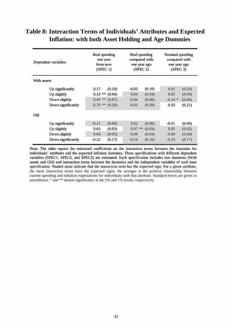
Table 8: Interaction Terms of Individuals’ Attributes and Expected Inflation: with both Asset Holding and Age Dummies

Note: The table reports the estimated coefficients on the interaction terms between the dummies forindividuals’ attributes and the expected inflation dummies. Three specifications with different dependentvariables (SPEC1, SPEC2, and SPEC3) are estimated. Each specification includes two dummies (Withassets and Old) and interaction terms between the dummies and the independent variables of each basespecification Shaded areas indicate that the interaction term has the expected sign For a given attribute


With assets

Up significantly 0.17 (0.10) -0.03 (0.10) 0.01 (0.10)Up slightly 0.10 ** (0.04) 0.04 (0.04) 0.05 (0.04)

Down slightly 0.45 ** (0.07) -0.04 (0.06) -0.14 * (0.06)Down significantly 0.76 ** (0.20) -0.03 (0.20) 0.03 (0.21)

Old

Up significantly -0.11 (0.06) 0.02 (0.06) -0.01 (0.06)

Up slightly 0.03 (0.03) 0.07 ** (0.03) 0.05 (0.02)Down slightly 0.04 (0.05) -0.00 (0.04) -0.00 (0.04)

Down significantly -0.22 (0.17) -0.16 (0.16) -0.23 (0.17)


from now(SPEC 1)


(SPEC 2)


(SPEC 3)

Note: The table reports the estimated coefficients on the interaction terms between the dummies forindividuals’ attributes and the expected inflation dummies. Three specifications with different dependentvariables (SPEC1, SPEC2, and SPEC3) are estimated. Each specification includes two dummies (Withassets and Old) and interaction terms between the dummies and the independent variables of each basespecification. Shaded areas indicate that the interaction term has the expected sign. For a given attribute,the more interaction terms have the expected signs, the stronger is the positive relationship betweencurrent spending and inflation expectations for individuals with that attribute. Standard errors are given inparentheses. * and ** denote significance at the 5% and 1% levels, respectively.


With assets

Up significantly 0.17 (0.10) -0.03 (0.10) 0.01 (0.10)Up slightly 0.10 ** (0.04) 0.04 (0.04) 0.05 (0.04)

Down slightly 0.45 ** (0.07) -0.04 (0.06) -0.14 * (0.06)Down significantly 0.76 ** (0.20) -0.03 (0.20) 0.03 (0.21)

Old

Up significantly -0.11 (0.06) 0.02 (0.06) -0.01 (0.06)

Up slightly 0.03 (0.03) 0.07 ** (0.03) 0.05 (0.02)Down slightly 0.04 (0.05) -0.00 (0.04) -0.00 (0.04)

Down significantly -0.22 (0.17) -0.16 (0.16) -0.23 (0.17)


from now(SPEC 1)


(SPEC 2)


(SPEC 3)

42

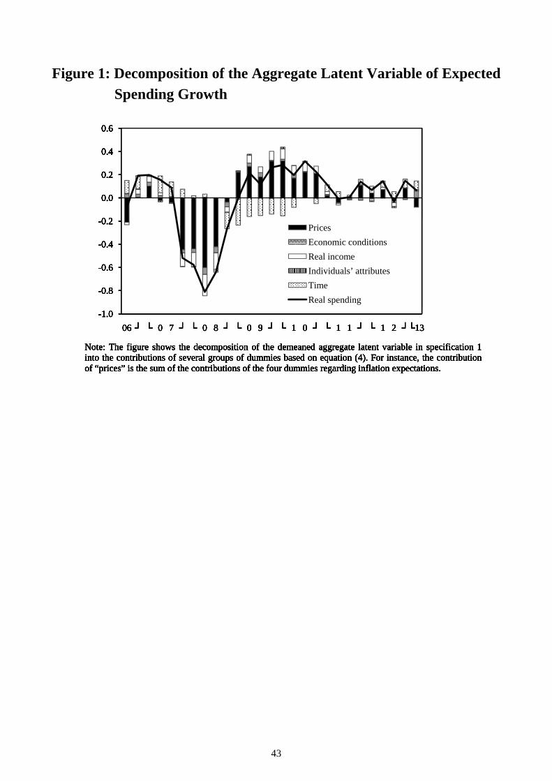
Figure 1: Decomposition of the Aggregate Latent Variable of Expected

Spending Growth

0 6

0 2

0.0

0.2

0.4

0.6

-0.8

-0.6

-0.4

-0.2

0.0

0.2

0.4

0.6

Prices

Economic conditions

Real income

Individuals’ attributes

Time

Real spending

-1.0

-0.8

-0.6

-0.4

-0.2

0.0

0.2

0.4

0.6

06 ┘ └ 0 7 ┘ └ 0 8 ┘ └ 0 9 ┘ └ 1 0 ┘ └ 1 1 ┘ └ 1 2 ┘└13

Prices

Economic conditions

Real income


Time

Real spending

Note: The figure shows the decomposition of the demeaned aggregate latent variable in specification 1into the contributions of several groups of dummies based on equation (4). For instance, the contributionof “prices” is the sum of the contributions of the four dummies regarding inflation expectations.

-1.0

-0.8

-0.6

-0.4

-0.2

0.0

0.2

0.4

0.6

06 ┘ └ 0 7 ┘ └ 0 8 ┘ └ 0 9 ┘ └ 1 0 ┘ └ 1 1 ┘ └ 1 2 ┘└13

Prices

Economic conditions

Real income


Time

Real spending


-1.0

-0.8

-0.6

-0.4

-0.2

0.0

0.2

0.4

0.6

06 ┘ └ 0 7 ┘ └ 0 8 ┘ └ 0 9 ┘ └ 1 0 ┘ └ 1 1 ┘ └ 1 2 ┘└13

Prices

Economic conditions

Real income


Time

Real spending


-1.0

-0.8

-0.6

-0.4

-0.2

0.0

0.2

0.4

0.6

06 ┘ └ 0 7 ┘ └ 0 8 ┘ └ 0 9 ┘ └ 1 0 ┘ └ 1 1 ┘ └ 1 2 ┘└13

Prices

Economic conditions

Real income


Time

Real spending


-1.0

-0.8

-0.6

-0.4

-0.2

0.0

0.2

0.4

0.6

06 ┘ └ 0 7 ┘ └ 0 8 ┘ └ 0 9 ┘ └ 1 0 ┘ └ 1 1 ┘ └ 1 2 ┘└13

Prices

Economic conditions

Real income


Time

Real spending


43

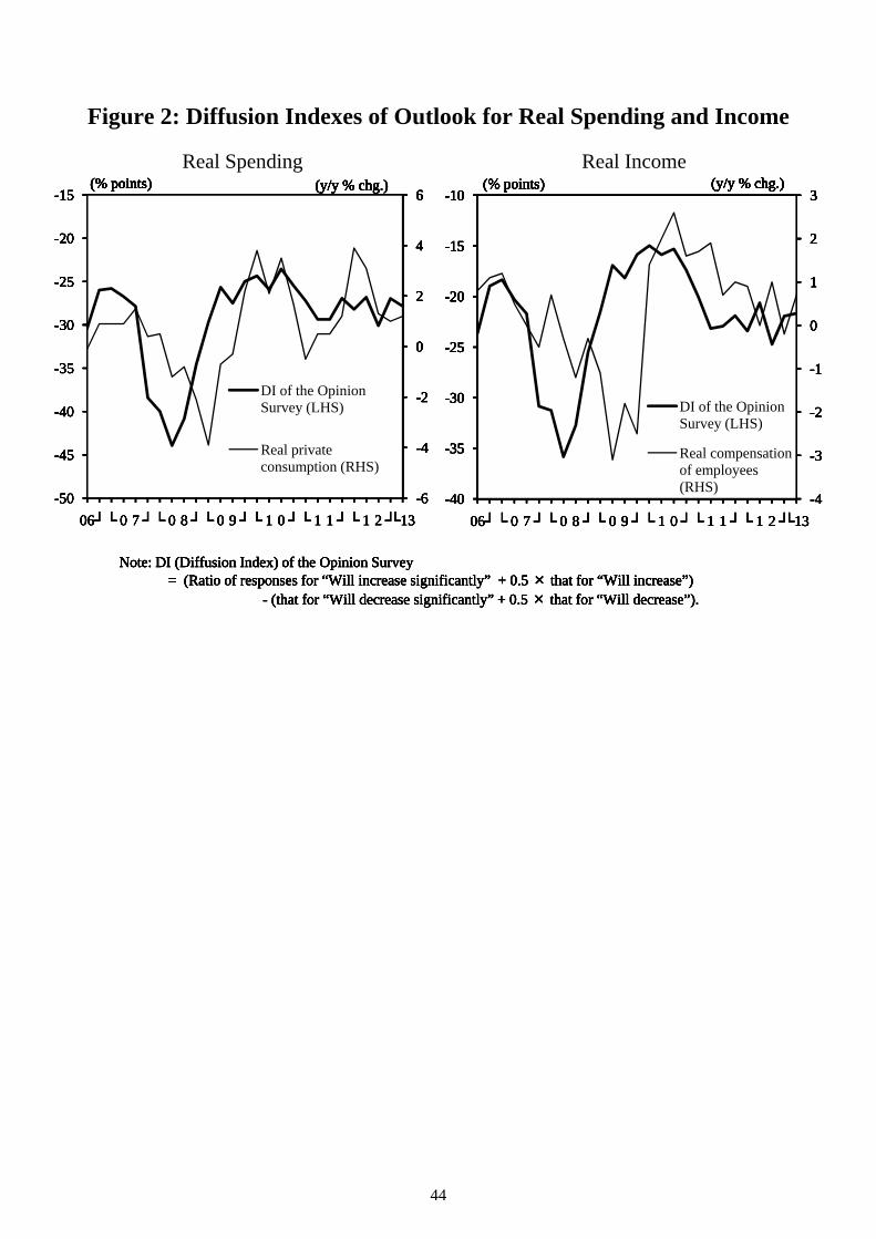
Figure 2: Diffusion Indexes of Outlook for Real Spending and Income

Real Spending Real Income

6-15(y/y % chg.)(% points)

3 -10(y/y % chg.)(% points)

0

2

4

6

-30

-25

-20

-15(y/y % chg.)(% points)

0

1

2

3

-25

-20

-15

-10(y/y % chg.)(% points)

-4

-2

0

2

4

6

-45

-40

-35

-30

-25

-20

-15

DI of the Opinion Survey (LHS)

Real private consumption (RHS)

(y/y % chg.)(% points)

-3

-2

-1

0

1

2

3

-35

-30

-25

-20

-15

-10


Real compensation of employees (RHS)


-6

-4

-2

0

2

4

6

-50

-45

-40

-35

-30

-25

-20

-15

06┘└ 0 7 ┘└ 0 8 ┘└ 0 9 ┘└ 1 0 ┘└ 1 1 ┘└ 1 2 ┘└13




-4

-3

-2

-1

0

1

2

3

-40

-35

-30

-25

-20

-15

-10

06┘└ 0 7 ┘└ 0 8 ┘└ 0 9 ┘└ 1 0 ┘└ 1 1 ┘└ 1 2 ┘└13




Note: DI (Diffusion Index) of the Opinion Survey= (Ratio of responses for “Will increase significantly” + 0.5 × that for “Will increase”)

- (that for “Will decrease significantly” + 0.5 × that for “Will decrease”).

-6

-4

-2

0

2

4

6

-50

-45

-40

-35

-30

-25

-20

-15

06┘└ 0 7 ┘└ 0 8 ┘└ 0 9 ┘└ 1 0 ┘└ 1 1 ┘└ 1 2 ┘└13




-4

-3

-2

-1

0

1

2

3

-40

-35

-30

-25

-20

-15

-10

06┘└ 0 7 ┘└ 0 8 ┘└ 0 9 ┘└ 1 0 ┘└ 1 1 ┘└ 1 2 ┘└13






-6

-4

-2

0

2

4

6

-50

-45

-40

-35

-30

-25

-20

-15

06┘└ 0 7 ┘└ 0 8 ┘└ 0 9 ┘└ 1 0 ┘└ 1 1 ┘└ 1 2 ┘└13




-4

-3

-2

-1

0

1

2

3

-40

-35

-30

-25

-20

-15

-10

06┘└ 0 7 ┘└ 0 8 ┘└ 0 9 ┘└ 1 0 ┘└ 1 1 ┘└ 1 2 ┘└13






-6

-4

-2

0

2

4

6

-50

-45

-40

-35

-30

-25

-20

-15

06┘└ 0 7 ┘└ 0 8 ┘└ 0 9 ┘└ 1 0 ┘└ 1 1 ┘└ 1 2 ┘└13




-4

-3

-2

-1

0

1

2

3

-40

-35

-30

-25

-20

-15

-10

06┘└ 0 7 ┘└ 0 8 ┘└ 0 9 ┘└ 1 0 ┘└ 1 1 ┘└ 1 2 ┘└13






-6

-4

-2

0

2

4

6

-50

-45

-40

-35

-30

-25

-20

-15

06┘└ 0 7 ┘└ 0 8 ┘└ 0 9 ┘└ 1 0 ┘└ 1 1 ┘└ 1 2 ┘└13




-4

-3

-2

-1

0

1

2

3

-40

-35

-30

-25

-20

-15

-10

06┘└ 0 7 ┘└ 0 8 ┘└ 0 9 ┘└ 1 0 ┘└ 1 1 ┘└ 1 2 ┘└13






44

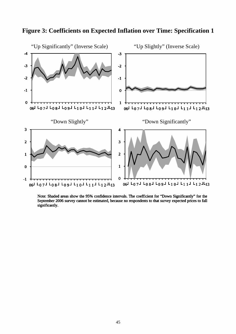
Figure 3: Coefficients on Expected Inflation over Time: Specification 1

“Up Significantly” (Inverse Scale) “Up Slightly” (Inverse Scale)-4 -3 -4

-3

-2

-1

-3

-2

-1

0

“Down Slightly” “Down Significantly”

-4

-3

-2

-1

0

06┘└ 0 7┘└ 0 8┘└ 0 9┘└ 1 0┘└ 1 1┘└ 1 2┘└13

-3

-2

-1

0

1

06┘└ 0 7┘└ 0 8┘└ 0 9┘└ 1 0┘└ 1 1┘└ 1 2┘└13

3 4

-4

-3

-2

-1

0

06┘└ 0 7┘└ 0 8┘└ 0 9┘└ 1 0┘└ 1 1┘└ 1 2┘└13

-3

-2

-1

0

1

06┘└ 0 7┘└ 0 8┘└ 0 9┘└ 1 0┘└ 1 1┘└ 1 2┘└13

0

1

2

3

1

2

3

4

-4

-3

-2

-1

0

06┘└ 0 7┘└ 0 8┘└ 0 9┘└ 1 0┘└ 1 1┘└ 1 2┘└13

-3

-2

-1

0

1

06┘└ 0 7┘└ 0 8┘└ 0 9┘└ 1 0┘└ 1 1┘└ 1 2┘└13

-1

0

1

2

3

06┘└ 0 7┘└ 0 8┘└ 0 9┘└ 1 0┘└ 1 1┘└ 1 2┘└13

0

1

2

3

4

06┘└ 0 7┘└ 0 8┘└ 0 9┘└ 1 0┘└ 1 1┘└ 1 2┘└13

Note: Shaded areas show the 95% confidence intervals. The coefficient for “Down Significantly” for theSeptember 2006 survey cannot be estimated, because no respondents to that survey expected prices to fallsignificantly.

-4

-3

-2

-1

0

06┘└ 0 7┘└ 0 8┘└ 0 9┘└ 1 0┘└ 1 1┘└ 1 2┘└13

-3

-2

-1

0

1

06┘└ 0 7┘└ 0 8┘└ 0 9┘└ 1 0┘└ 1 1┘└ 1 2┘└13

-1

0

1

2

3

06┘└ 0 7┘└ 0 8┘└ 0 9┘└ 1 0┘└ 1 1┘└ 1 2┘└13

0

1

2

3

4

06┘└ 0 7┘└ 0 8┘└ 0 9┘└ 1 0┘└ 1 1┘└ 1 2┘└13


-4

-3

-2

-1

0

06┘└ 0 7┘└ 0 8┘└ 0 9┘└ 1 0┘└ 1 1┘└ 1 2┘└13

-3

-2

-1

0

1

06┘└ 0 7┘└ 0 8┘└ 0 9┘└ 1 0┘└ 1 1┘└ 1 2┘└13

-1

0

1

2

3

06┘└ 0 7┘└ 0 8┘└ 0 9┘└ 1 0┘└ 1 1┘└ 1 2┘└13

0

1

2

3

4

06┘└ 0 7┘└ 0 8┘└ 0 9┘└ 1 0┘└ 1 1┘└ 1 2┘└13


-4

-3

-2

-1

0

06┘└ 0 7┘└ 0 8┘└ 0 9┘└ 1 0┘└ 1 1┘└ 1 2┘└13

-3

-2

-1

0

1

06┘└ 0 7┘└ 0 8┘└ 0 9┘└ 1 0┘└ 1 1┘└ 1 2┘└13

-1

0

1

2

3

06┘└ 0 7┘└ 0 8┘└ 0 9┘└ 1 0┘└ 1 1┘└ 1 2┘└13

0

1

2

3

4

06┘└ 0 7┘└ 0 8┘└ 0 9┘└ 1 0┘└ 1 1┘└ 1 2┘└13


45

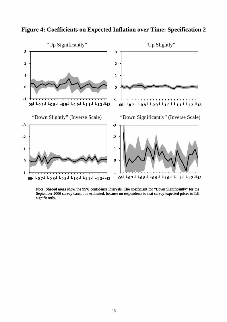
Figure 4: Coefficients on Expected Inflation over Time: Specification 2

“Up Significantly” “Up Slightly”3 3

0

1

2

3

0

1

2

3

“Down Slightly” (Inverse Scale) “Down Significantly” (Inverse Scale)

-1

0

1

2

3

06┘└ 0 7┘└ 0 8┘└ 0 9┘└ 1 0┘└ 1 1┘└ 1 2┘└13

-1

0

1

2

3

06┘└ 0 7┘└ 0 8┘└ 0 9┘└ 1 0┘└ 1 1┘└ 1 2┘└13

-3 -3

-1

0

1

2

3

06┘└ 0 7┘└ 0 8┘└ 0 9┘└ 1 0┘└ 1 1┘└ 1 2┘└13

-1

0

1

2

3

06┘└ 0 7┘└ 0 8┘└ 0 9┘└ 1 0┘└ 1 1┘└ 1 2┘└13

-3

-2

-1

0

-3

-2

-1

0

-1

0

1

2

3

06┘└ 0 7┘└ 0 8┘└ 0 9┘└ 1 0┘└ 1 1┘└ 1 2┘└13

-1

0

1

2

3

06┘└ 0 7┘└ 0 8┘└ 0 9┘└ 1 0┘└ 1 1┘└ 1 2┘└13

-3

-2

-1

0

1

06┘└ 0 7┘└ 0 8┘└ 0 9┘└ 1 0┘└ 1 1┘└ 1 2┘└13

-3

-2

-1

0

1

06┘└ 0 7┘└ 0 8┘└ 0 9┘└ 1 0┘└ 1 1┘└ 1 2┘└13


-1

0

1

2

3

06┘└ 0 7┘└ 0 8┘└ 0 9┘└ 1 0┘└ 1 1┘└ 1 2┘└13

-1

0

1

2

3

06┘└ 0 7┘└ 0 8┘└ 0 9┘└ 1 0┘└ 1 1┘└ 1 2┘└13

-3

-2

-1

0

1

06┘└ 0 7┘└ 0 8┘└ 0 9┘└ 1 0┘└ 1 1┘└ 1 2┘└13

-3

-2

-1

0

1

06┘└ 0 7┘└ 0 8┘└ 0 9┘└ 1 0┘└ 1 1┘└ 1 2┘└13


-1

0

1

2

3

06┘└ 0 7┘└ 0 8┘└ 0 9┘└ 1 0┘└ 1 1┘└ 1 2┘└13

-1

0

1

2

3

06┘└ 0 7┘└ 0 8┘└ 0 9┘└ 1 0┘└ 1 1┘└ 1 2┘└13

-3

-2

-1

0

1

06┘└ 0 7┘└ 0 8┘└ 0 9┘└ 1 0┘└ 1 1┘└ 1 2┘└13

-3

-2

-1

0

1

06┘└ 0 7┘└ 0 8┘└ 0 9┘└ 1 0┘└ 1 1┘└ 1 2┘└13


-1

0

1

2

3

06┘└ 0 7┘└ 0 8┘└ 0 9┘└ 1 0┘└ 1 1┘└ 1 2┘└13

-1

0

1

2

3

06┘└ 0 7┘└ 0 8┘└ 0 9┘└ 1 0┘└ 1 1┘└ 1 2┘└13

-3

-2

-1

0

1

06┘└ 0 7┘└ 0 8┘└ 0 9┘└ 1 0┘└ 1 1┘└ 1 2┘└13

-3

-2

-1

0

1

06┘└ 0 7┘└ 0 8┘└ 0 9┘└ 1 0┘└ 1 1┘└ 1 2┘└13


46

inflation expectations and consumer spending at … expectations and consumer spending at the zero...

Documents