inflation expectations, real rates, and risk premia...

Inflation Expectations, Real Rates, and RiskPremia: Evidence from Inflation Swaps

Joseph HaubrichFederal Reserve Bank of Cleveland

George PennacchiFederal Reserve Bank of Cleveland and University of Illinois

Peter RitchkenCase Western Reserve University, Weatherhead School of Management,Federal Reserve Bank of Cleveland

We develop a model of nominal and real bond yield curves that has four stochasticdrivers but seven factors: three factors primarily determine the cross-section of yields,whereas four volatility factors solely determine risk premia. The model is estimatedusing nominal Treasury yields, survey inflation forecasts, and inflation swap rates and hasattractive empirical properties. Time-varying volatility is particularly apparent in short-term real rates and expected inflation. Also, we detail the different economic forcesthat drive short- and long-term real and inflation risk premia and provide evidence thatTreasury inflation-protected securities were undervalued prior to 2004 and during therecent financial crisis. (JELG01, G12, G13)

Policymakers and finance professionals often use the term structure of Trea-sury yields to infer expectations of inflation and real interest rates. Inflationexpectations can gauge the credibility of a government’s fiscal and mon-etary policies, whereas real rates measure the economic cost of financinginvestments and the tightness of monetary policy. However, Treasury yieldsembed time-varying risk premia that make it difficult to extract measures ofexpected inflation and real rates. This article presents a new methodologyfor decomposing Treasury yields and analyzes the determinants of the termstructures of real rates, expected inflation, and inflation risk premia. The article

Theviews expressed in this article do not necessarily represent those of the Federal Reserve Bank of Clevelandor the Federal Reserve System. For valuable comments, we thank Editor Pietro Veronesi and an anonymousreferee, as well as seminar participants at the Hong Kong University of Science and Technology, NanyangTechnical University, National University of Singapore, Singapore Management University, University ofArizona, University of Hong Kong, and University of Oklahoma. Helpful suggestions were also provided byparticipants of the Federal Reserve Bank of New York’s Conference on Inflation-indexed Securities and InflationRisk Management, especially our discussant Mikhail Chernov. Send correspondence to George Pennacchi,University of Illinois College of Business, 4041 BIF, 515 East Gregory Drive, Champaign, IL 61820; telephone:(217) 244-0952. E-mail: [email protected].

c© The Author 2012. Published by Oxford University Press on behalf of The Society for Financial Studies.All rights reserved. For Permissions, please e-mail: [email protected]:10.1093/rfs/hhs003 Advance Access publication March 5, 2012

at Com

merce L

ibrary on April 15, 2012

http://rfs.oxfordjournals.org/D

ownloaded from

http://rfs.oxfordjournals.org/

InflationExpectations, Real Rates, and Risk Premia: Evidence from Inflation Swaps

hastwo main innovations relative to the existing literature. First, it develops anew model of nominal and real term structures that provides a convenient,yet realistic, framework for identifying the dynamics of real and inflation-related factors. Second, the article introduces a new data source for estimatingsuch models, namely, zero-coupon inflation swaps. We present evidence thatthe difference between nominal yields and inflation swap rates provides morereliable information on real yields than do inflation-indexed bond yields.

Our model of nominal and real term structures has several desirable prop-erties. It generates simple, closed-form solutions for nominal yields, inflation-indexed yields, inflation swap rates, and expected inflation that make empiricalestimation straightforward. Furthermore, it is consistent with two importantempirical properties of nominal yields: yields have stochastic volatilities thatare correlated with their levels (Ait-Sahalia 1996;Brenner, Harjes, and Kroner1996;Gallant and Tauchen 1998); and risk premia (expected excess returns)on longer-maturity bonds are highest when the yield curve is steep (Famaand Bliss 1987;Campbell and Shiller 1991). Since it captures the relevantempirical features of nominal yields, the model is likely to provide a correctstarting point for decomposing these yields into real rates, expected inflation,and risk premia.

It may be surprising that our term structure model is in the completely affineclass.Dai and Singleton(2000) show that many completely affine modelsfail to possess important empirical features of nominal yields.1 However, ourmodel is outside the subclass that they studied and differs because it has fourstochastic drivers (sources of risk) yetsevenstate variables. Three of the statevariables are the short-term real interest rate, expected inflation, and inflation’s“central tendency,” and they have a large influence on the cross-section ofbond yields. However, they play no direct role in determining bonds’ riskpremia. Rather, bond risk premia depend on four volatility-state variables thathave dynamics driven by normal and chi-squared innovations that derive frominflation and the aforementioned three state variables. This decoupling of thestate variables that largely determine the cross-section of yields, versus thosethat solely determine risk premia, allows for time-varying risk premia that caneven change sign.2 As a result, the model’s ability to fit the cross-section andtime-series of yields exceeds that of traditional affine models.

The article’s second main innovation is its use of data on inflation swaprates, in addition to nominal Treasury yields and survey forecasts of inflation,

1 In response to limitations of completely affine models,Duffee (2002) andDai and Singleton(2000) developmore general “essentially affine” models that permit time-varying risk premia capable of producing positivecorrelation between bond excess returns and the slope of the yield curve. This feature occurs when the models’state variables are Gaussian, but such models cannot capture the equally well-established time variation in yields’volatilities that are positively related to their levels.

2 Different from the usual completely affine models, our model has market prices of risk that are neither constant,as inVasicek(1977), nor proportional to the square root of variables that directly affect the levels of yields, asin Cox, Ingersoll, and Ross(1985).

1589

at Com

merce L



ownloaded from


TheReview of Financial Studies / v 25 n 5 2012

to estimate the model’s parameters. Identifying the parameters of a joint modelof nominal and real term structures requires more than just data on nominalyields. Previous work using U.S. data typically employs nominal Treasuryyields along with either Treasury inflation-protected securities (TIPS) yields(D’Amico, Kim, and Wei 2008; Chen, Liu, and Cheng 2010; Christensen,Lopez, and Rudebusch 2010) or survey forecasts of inflation (Pennacchi1991; Chernov and Mueller,forthcoming).3,4 Unlike most studies, we usethree different sources of data. We show that inflation-indexed yields canbe computed as the difference between equivalent maturity nominal Treasuryyields and inflation swap rates, and these derived real yields are less prone toliquidity shocks than are TIPS yields. Consequently, model estimation usinginflation swap rates, rather than TIPS yields, leads to more reliable parameterestimates. Whereas using survey inflation forecasts, in addition to nominalyields and inflation swaps, creates extra demands on our model’s ability tomatch all observations, it permits better identification of physical expectationsof inflation (as reflected in survey forecasts) versus inflation risk premia (asreflected in nominal yields).

Based on the estimated model, we are able to compute term structures ofinflation expectations and inflation-indexed (real) yields over our entire 1982-to-2010 sample period. Comparing our model-implied real yields to TIPSyields beginning in 1999, we confirm the results of prior studies that foundmassive underpricing of TIPS during their early years, followed by fair pricingfrom 2004 to 2008. Enormous underpricing of TIPS reappeared during the2008-to-2009 financial crisis years.

We obtain several other noteworthy results. First, we find that the short-term real interest rate is typically the most volatile component of the yieldcurve, and it is especially important to allow its volatility to be stochastic.Real rates were negative for much of 2002 to 2005, which may have helpedinflate a credit bubble. Second, we find that expected inflation over shorthorizons is also volatile and has high negative correlation with real rates,likely an artifact of the Federal Reserve’s policy of pegging short-termnominal interest rates. Moreover, both real rates and expected inflation displaystrong mean reversion. Third, over our 1982-to-2010 sample period, inflation’scentral tendency, which can be viewed as investors’ expectation of longer-term inflation, declined substantially, consistent with greater credibility of theFederal Reserve’s desire to maintain low inflation.

3 Similarly, Barr and Campbell(1997) andEvans(1998) use British nominal and index-linked gilt yields, andHordahl and Tristani(2007) use euro-denominated nominal and inflation-indexed bond yields.

4 Ang, Bekaert, and Wei(2007) develop a regime-switching model that is estimated using data on nominal yieldsand actual inflation. Identification is acheived by inferring expected inflation from the actual inflation processalong with imposing other parameter restrictions. Similarly,Buraschi and Jiltsov(2005) develop a structuralmonetary model, whose parameters are estimated using data on nominal yields and the processes for actualinflation and the M2 money supply.

1590

at Com

merce L



ownloaded from



Our last results explain the term structures of real and inflation risk premia,which are solely determined by the model’s four volatility-state variables. Realrisk premia averaged 25, 57, and 103 basis points for two-, five-, and ten-year maturities, respectively. We show that shorter-maturity real risk premiaincrease when the volatility of the short-term real rate is high. However,increases in longer-maturity real risk premia occur mainly with a rise in thevolatility of inflation’s central tendency, reflecting possible nonneutrality inlonger-run inflation. We also estimate an inflation risk premium that averaged−5, 17, and 44 basis points for two-, five-, and ten-year maturities. Atshort maturities, inflation risk premia are inversely related to the volatilityof unanticipated inflation or deflation. This volatility factor also reduceslonger-maturity inflation risk premia during financial crises when there is a“flight-to-quality.” During normal times, however, longer-maturity inflationrisk premia are more positively related to the volatility of inflation’s centraltendency. These results accord with economic intuition regarding how differentsources of real and inflation uncertainty affect the term structure of riskpremia.

The article proceeds as follows. Section1 introduces a model of real interestrates and inflation that is used to derive the term structures of nominal bonds,inflation forecasts, inflation-indexed bonds, and inflation swap rates. Section2 describes the data used and explains the estimation technique. Section3describes the results, and Section4 concludes.

1. A Model of Nominal and Real Term Structures

Consider a discrete time environment with multiple periods, each of lengthΔtmeasured in years. LetMt bethe nominal pricing kernel with dynamics

Mt+Δt

Mt= e−i tΔt− 1

2

∑4j =1 φ2

j h2j,tΔt−

∑4j =1 φ j h j,t

√Δtε j,t+Δt . (1)

Here, ε j,t+Δt , j = 1,2, . . . , 4 are independent standard normal randomvariables andφ j h j,t , j = 1,2, . . . , 4 are market prices of risk associated withthese four sources of uncertainty. Theφ j areconstants, whereas theh j,t arevolatility-state variables whose dynamics will be specified shortly.i t is theannualized, one-period nominal interest rate.

Denote the consumer price index (dollar value of the consumption basket)at datet as It . Its dynamics are

It+Δt

It= eπtΔt− 1

2h21,tΔt+h1,t

√Δtε1,t+Δt , (2)

whereπt = 1Δt ln

(Et[It+Δt/It

])is the rate of expected inflation fromt to

t + Δt .

1591

at Com

merce L



ownloaded from



Therefore,the process for the real (inflation-indexed) pricing kernel,mt , is

mt+Δt

mt=

Mt+Δt

Mt

It+Δt

It(3)

= e

(πt−i t− 1

2h21,t

)Δt− 1

2

∑4j =1 φ2

j h2j,tΔt−

∑4j =1 φ j h j,t

√Δtε j,t+Δt +h1,t

√Δtε1,t+Δt .

Taking expectations of the left-hand side of Equation (3) definesrt , the one-period real rate:

Et

[mt+Δt

mt

]= e−rtΔt . (4)

Taking expectations on the right-hand side of Equation (3) and equating it toEquation (4) implies that

i t = πt + rt − φ1h21,t . (5)

To complete the model, the dynamics of the state variables are specified as

πt+Δt − πt = [αt + a1rt + a2πt ] Δt +√ΔtΣ2

j =1β j h j,tε j,t+Δt

r t+Δt − rt = [b0 + b1rt + b2πt ] Δt +√ΔtΣ3

j =1γ j h j,tε j,t+Δt

αt+Δt − αt = [c0 + c1αt ] Δt +√ΔtΣ4

j =1ρ j h j,tε j,t+Δt

h2j,t+Δt − h2

j,t =[dj 0 + dj 1h2

j,t

]Δt

+dj 2Δt (ε j,t+Δt − dj 3h j,t )2, j = 1, . . . , 4, (6)

whereαt is an additional state variable that shifts the future path ofπt . Subjectto stationarity conditions, the unconditional means (steady-state levels) ofπt

andrt are

π= −a1b0c1 + b1c0

(a1b2 − a2b1) c1, (7)

r =a2b0c1 + b2c0

(a1b2 − a2b1) c1. (8)

The unconditional mean ofαt is−c0/c1 = −(a1r +a2π). If a constant is addedto αt suchthatαt ≡ αt + a1r + (1 + a2)π, then the unconditional mean ofαt

equalsπ, andαt is commonly referred to as the “central tendency” of the rateof expected inflation.5 For simplicity, we refer toαt asthe central tendency,but it should be understood that it differs from the true central tendency,αt , bya constant.

5 Prior research supports a time-varying central tendency for inflation in order to adequately fit the term structure(Balduzzi, Das, and Foresi 1998; Jegadeesh and Pennacchi 1996).Kozicki and Tinsley(2009) show that a“shifting endpoint” for the short-term interest rate process captures historical changes in market perceptionsof the policy target for inflation and significantly improves long-horizon forecasts of short-term interest rates.

1592

at Com

merce L



ownloaded from



The h j,t arevolatility-state variables that satisfy the nonlinear asymmetricGARCH model ofEngle and Ng(1993). Subject to stationarity conditions,their steady states are

h2j = −

dj 0 + dj 2

dj 1 + dj 2d2j 3

, j = 1, . . . , 4. (9)

Equations (2) and (6) specify that actual inflation, expected inflation, thereal interest rate, and inflation’s central tendency follow imperfectly correlated,stochastic volatility processes. Their correlations depend on theβ j , γ j , andρ j

coefficients multiplying the four orthogonal shocks,h j,tε j,t+Δt , j = 1, . . . , 4,but without loss of generality, we can restrictβ2 = γ3 = ρ4 = 1. If the fourvolatility-state variables are shut down, the model becomes Gaussian in thethree state variables,πt , rt , andαt .6

Themodel’s state variables can be written as a 7×1 vectorxt ≡ (πt r t αt h21t

h22t h2

3t h24t)

′, whereas the market prices of risk associated with each of the fourshocksh j,tε j,t+Δt , j = 1, . . . , 4 are the 4×1 vectorΛt ≡ (φ1h1t φ2h2t φ3h3t

φ4h4t)′. The compensation for risk depends on the square roots of theh2

j,t statevariables but not the other state variables. Furthermore, because the processesfor the h2

j,t statevariables depend on both the levels of the innovations,ε j,t ,

andtheir squares,ε2j,t , the datet + Δt distribution of the state vectorxt+Δt

conditionalon xt is not multivariate normal but a mixture of normals and chi-squared distributions. Since bond yields are shown to be affine inxt , yieldchanges will display the skewness and kurtosis derived fromxt .

AsΔt → 0, our model can be made to converge to many possible diffusivelimits. The proposition below describes one possible case.

Proposition 1. If we definedj 0 = (κ j θ j −v2

j4 ) , dj 1 = − 1

Δt , dj 2 =v2

j4 , and

dj 3 =2(1−κ jΔt/2)

v j√Δt

, then the limiting dynamics of Equation (6) is

dπt = (αt + a1rt + a2πt )dt + Σ2j =1β j h j,t dWj (t)

drt = (b0 + b1rt + b2πt )dt + Σ3j =1γ j h j,t dWj (t)

dαt = (c0 + c1αt )dt + Σ4j =1ρ j h j,t dWj (t)

dh2j,t = κ j (θ j − h2

j,t )dt − v j

√h2

j,t dWj (t), j = 1, . . . ,4, (10)

wheredWj t , j = 1, . . . , 4 are independent Wiener processes.

Proof. See Appendix.

6 This “no GARCH” case occurs whendj 1 = −1/Δt anddj 2 = dj 3 = 0, so thath2j,t = h

2j ∀t .

1593

at Com

merce L



ownloaded from



Whereasour empirical model assumes a period of one month (Δt= 1/12),it may be interpreted as approximating the above continuous-time, stochasticvolatility model. �

1.1 Nominal and inflation-indexed bondsThe model is estimated using data on nominal Treasury yields, inflation swaprates, and survey forecasts of inflation. This section derives model prices fornominal and inflation-indexed (real) bonds, which also determine inflationswap rates. The following section gives the model formula for inflationforecasts.

Let P(n)N,t and y(n)

N,t be the datet price and continuously compounded yield,respectively, of a nominal bond that pays one dollar at datet + nΔt . Similarly,P(n)

R,t andy(n)R,t arethe datet real price and yield of a bond that pays one unit of

the consumption basket at datet + nΔt . In practice, an inflation-indexed bondtypically pays semi-annual coupons, but since its payments are a portfolio ofzero-coupon payments, it is sufficient to value a zero-coupon inflation-indexedbond. Moreover, inflation-indexed payments are not fully protected againstinflation. For example, the inflation index for a TIPS payment is based on theconsumer price index (CPI) recorded three months prior to the payment date.7

Accountingfor this indexation lag, defineV (n,d)t,ts asthe datet nominal price

of a zero-coupon TIPS that hasn periods until its payment at date oftp =t + nΔt . Let t0 be this bond’s issue date, and letd be the indexation lag inperiods. Following actual practice, the payment made at datetp is based onaccumulated inflation from datests ≡ t0 − dΔt to te ≡ tp − dΔt . Thus, thepayment at datetp equalsaccumulated inflation,Ite/Its, over the life of thebond but laggedd periods. For TIPS,dΔt = 3 × 1/12 = 1

4 year. Note that atdatete, the value of the payment maded periods later is

V (d,d)te,ts =

Ite

ItsP(d)

N,te, (11)

and at datet , with n periods to go to datetp, we have

V (n,d)t,ts = Et

[Mt+Δt

MtV (n−1,d)

t+Δt,ts

]. (12)

SinceV (n,d)t,ts is the datet nominal price of receivingIte/Its dollarsat datetp,

V (n,d)t,ts Its is the nominal price of receivingIte dollarsat datetp. If P(n,d)

R,t isdefinedto be the datet real price of receivingIte dollarsat datetp, then

P(n,d)R,t = V (n,d)

t,ts

Its

It. (13)

7 A reason for this delay is that the CPI is reported with a lag after the date for which it is recorded. Most modelsignore this indexation lag, thoughRisa(2001) is an exception.

1594

at Com

merce L



ownloaded from



With no indexation delay (d = 0), P(n,0)R,t = P(n)

R,t representsthe real price ofa claim that pays one unit of the consumption basket inn periods.

Inflation Swaps“Zero-coupon inflation swaps” are the most liquid of all the over-the-countermarket inflation derivative products. They are quoted with maturities rangingfrom one to 30 years. Together with nominal Treasuries, they provide analternative measure of real yields.

A zero-coupon inflation swap is a forward contract, whereby the inflationbuyer pays a predetermined fixed nominal rate and in return receives from theseller an inflation-linked payment. Denote the swap’s initiation date ast0 andits maturity (payment) date astp. Similar to TIPS, the inflation-linked paymentmade at datetp equalsIte/Its, where, as before,ts = t0 − dΔt , te ≡ tp − dΔt ,anddΔt = 1

4 years.In return for receivingIte/Its, the inflation buyer makes afixed payment ofek(te−ts), wherek is the continuously compounded inflationswap rate.8 Thus,the net fixed for inflation swap payment isek(te−ts)− Ite/Its.

Viewed from datet , the value of the fixed (nominal) leg is simply

Vf ix (t) = P(n)N,t e

k(te−ts). (14)

The value of the inflation leg, sayVinf (t), equals the value of a zero-couponTIPS with payouts at datetp linked to the index values at datests andte:

Vinf (t) = V (n,d)t,ts = P(n,d)

R,tIt

Its. (15)

At the initiation date,t0, the fair swap rate is that which equatesVf ix (t0) toVinf (t0):

k∗(t0; ts, te) = y(n)N,t0

− y(n,d)R,t0

= be(n,d)t0 , (16)

wherey(n,d)R,t0

is defined as

y(n,d)R,t0

= −1

nΔtln V (n,d)

t0,ts = −1

nΔtln(

P(n,d)R,t0

It0/Its

), (17)

andbe(n,d)t is the datet break-even inflation rate for a maturity ofnΔt years.

The above shows that once we have a valuation equation for a TIPS, we alsohave a value for a fair inflation swap rate. Moreover,y(n)

N,t0− k∗(t0; ts, te) =

y(n,d)R,t0

is a measure of ann-period maturity real yield that is an alternative to aTIPS yield.

The following proposition provides the recursive equations for both nominaland real (e.g., TIPS) bond values, which in turn can be used to value inflationswaps.

8 In practice, inflation swap rates are quoted as annually compounded rates, sayka, whereka = ln (k) − 1. Wetranslate these rates to continuously compounded ones.

1595

at Com

merce L



ownloaded from



Proposition 2. Under the above dynamics, nominal and real bond prices aregiven by

P(n)N,t = e−Kn−Anπt−Bnrt−Cnαt−

∑4j =1 D j,nh2

j,t for n ≥ 1, (18)

P(n,d)R,t = e−Kn−Anπt−Bnrt−Cnαt−

∑4j =1 D j,nh2

j,t for n ≥ d, (19)

whereK1 = 0, A1 = Δt , B1 = Δt , C1 = 0, D1,1 = −φ1Δt , D j,1 = 0 for

j = 2,3,4, andKd = Kd, Ad = Ad, Bd = Bd, Cd = Cd, D j,d = D j,d forj = 1,2,3,4, and the recursive equations are contained in the Appendix.

Proof. See the Appendix. �

1.2 Expected inflation ratesOur model’s parameters are estimated with data that include survey forecastsof an inflation rate that begins and ends at two future dates. If the current dateis t , whereast + nΔt andt + (n + m)Δt are the dates when the inflation ratestarts and ends, then the forecast of this continuously compounded inflationrate is9

Et

[1

mΔtln

(It+(n+m)Δt

It+nΔt

)]=

1

mΔt

(Et

[ln

(It+(n+m)Δt

It

)]

−Et

[ln

(It+nΔt

It

)]), (20)

which is the difference between expectations of an inflation rate over twodifferent horizons. Proposition 3 provides the formula for such an expectedrate of inflation.

Proposition 3. The datet expectation of the inflation rate for a horizon ofnperiods is

Et [ln (It+nΔt/It )] = K ∗n + A∗

nπt + B∗nrt + C∗

nαt + Σ4j =1D∗

j,nh2j,t for n ≥ 1,

(21)

whereK ∗1 = 0, A∗

1 = Δt , B∗1 = 0, C∗

1 = 0, D∗1,1 = −1

2Δt , andD∗j,1 = 0, for

j = 2,3,4, and where the recursions are provided in the Appendix.

Proof. See the Appendix. �The Appendix shows that the market price of risk parameters,φ j , j =

1, . . . , 4, appear in the formulas for nominal and inflation-indexed yields(including swap rates), but are absent from the formula for a forecastedinflation rate. A benefit of combining data that reflect risk premia and datathat do not is better identification of parameters that determine expectations ofstate variables versus those that characterize risk premia.

9 For example,m = 3 monthswhen the forecasted inflation rate is for a future quarter of a year.

1596

at Com

merce L



ownloaded from



2. Data and Estimation Method

2.1 Data descriptionOur model is estimated with monthly data on U.S. nominal Treasury yields,survey inflation forecasts, rates of actual inflation, and inflation swap rates.Most data series are from January 1982 to May 2010, though inflation swapdata only start in April 2003. Nominal Treasury yields come from two sources.First, zero-coupon yields of one, two, three, five, seven, ten, and 15 years tomaturity are obtained from daily off-the-run Treasury yield curves constructedby Gurkaynak, Sack, and Wright(2007). Second, daily secondary marketyields for one-, three-, and six-month Treasury bills are taken from the FederalReserve’s H.15 release. All Treasury yields are observed at the first trading dayof each month.

Survey forecasts of CPI inflation come from two sources. First, a monthlyseries beginning in 1982 is obtained from Blue Chip Economic Indicators(BCEI), which surveys approximately 50 economists employed by financialinstitutions, nonfinancial corporations, and research organizations. At the be-ginning of each month, participants forecast future CPI inflation for quarterlytime periods, starting from the current calendar quarter and going out to at mosteight quarters (two years) in the future. For January, February, and March,inflation rate forecasts for eight future quarters are made. For April, May,and June, forecasts for seven future quarters are made. For July, August, andSeptember, forecasts for six future quarters are made, whereas for October,November, and December, forecasts for five future quarters are made. We useBCEI’s reported “consensus” forecast, which is the average of the participants’forecasts.

Second, we use the median forecast of CPI inflation over the next tenyears made by the approximately 40 participants of the Survey of ProfessionalForecasters (SPF). This ten-year forecast is at a quarterly frequency, startingin December 1991.10 Ang, Bekaert, and Wei(2007) find that SPF forecastssignificantly outperform a variety of other methods for predicting inflation.Since the participants in the BCEI survey have qualifications similar to thoseof the SPF participants, BCEI forecasts should also possess these attractivefeatures. Along with both sets of survey forecasts of inflation, we alsoconstructed a monthly time series of actual CPI inflation.11

In addition, we obtained bid and ask quotes of inflation swap rates for thefirst trading day of each month from Bloomberg for annual maturities from twoto ten years, as well as for 12-, 15-, 20-, and 30-year maturities. The two- toten-year swap maturities start in April 2003; the 12-, 15-, and 20-year inflation

10 SPFforecasts are made at about the middle of February, May, August, and November. To align this survey withour other data, these forecasts are assumed to be at the start of the next month.

11 Survey forecasts are of seasonally adjusted CPI inflation, so our actual monthly CPI series is also seasonallyadjusted. However, TIPS and zero-coupon inflation swaps are indexed to the seasonally unadjusted CPI. Thisdifference likely has little impact on TIPS yields and swap rates, except perhaps for those of very short maturities.

1597

at Com

merce L



ownloaded from



swap rates start in November 2003; and the 30-year inflation swap rates startin March 2004.

Though not used to estimate our model, yields on TIPS will be comparedto our model’s implied yields for inflation-indexed bonds. Zero-coupon TIPSyields were obtained from Gurkaynak, Sack, and Wright (2008), who derivethem from TIPS coupon bond yields.

Table1 shows summary statistics of our data. Panel A describes the levelsand standard deviations of changes of nominal Treasury yields from 1982 to2010. The term structure of average nominal yields is upward sloping, andthe standard deviation of yield changes declines with maturity, consistent withmean reversion in short-term yields. Panel B shows similar statistics for surveyinflation forecasts. Blue Chip Economic Indicators inflation forecasts averagedslightly over 3% from 1982 to 2010, whereas the SPF forecasts during the1991-to-2010 period averaged 2.73%. The standard deviation of changes inforecasts mostly declined with maturity. The one-month forecast was volatile,which might reflect participants’ predictions of how commodity price swingswould affect next month’s consumer prices.

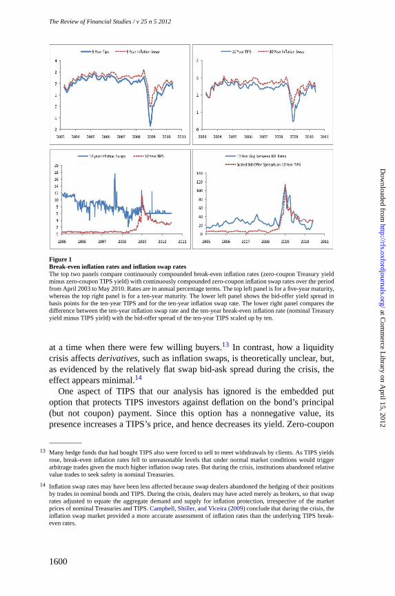
Panel C of Table1 gives statistics on the levels (midpoint of bid-askquotes) and changes of inflation swap rates during the 2003-to-2010 period.The standard deviations of monthly changes generally decline with maturity,and correlations decline as the gap between maturities increase. The averagelevels of rates increased with maturity, consistent with a positive inflation riskpremium. Recall from Equation (16) that in a frictionless market, inflationswap rates should equal the difference between equivalent-maturity, zero-coupon nominal Treasury and TIPS yields, i.e., the TIPS break-even inflationrate. Because we are unaware of any prior studies that have used inflationswap rates in term structure estimation, we detail in Figure1 how swap ratescompare to TIPS break-even rates. The top two panels in Figure1 plot theinflation swap rates and TIPS break-even rates for five- and ten-year maturitiesover the April 2003 to June 2010 period.

As can be seen, the difference between the inflation swap rate and the TIPSbreak-even rate was fairly stable, perhaps reflecting the cost of replication, untilthe financial crisis. But during the crisis, this relation became distorted.12 Thesolid curve in the bottom right panel of Figure1 shows the gap between theinflation swap rate and the TIPS break-even rate. This gap was fairly flat untilthe Lehman Brothers bankruptcy in September 2008, after which it increaseddramatically by about 60 basis points.

What accounted for this break in historical relations? The bottom left panelof Figure1 compares the bid-ask spread of ten-year inflation swap rates withthe bid-ask spread of the ten-year TIPS, both series obtained from Bloomberg.

12 Fleckenstein, Longstaff, and Lustig(2010) find that Treasury supply-related factors affect the difference betweeninflation swap rates and TIPS break-even rates. The difference narrows when the U.S. auctions either nominalTreasuries or TIPS, but it widens when dealers have difficulties obtaining Treasury securities, such as during aperiod of increased repo failures.

1598

at Com

merce L



ownloaded from



Table 1Summary statistics

Panel A: Nominal Treasury yieldsMaturity Average Minimum Maximum Std. Dev.

1 month 0.0475 0.0003 0.1347 0.02433 months 0.0507 0.0006 0.1431 0.01346 months 0.0517 0.0015 0.1457 0.01221 year 0.0546 0.0029 0.1437 0.01202 years 0.0578 0.0065 0.1440 0.01253 years 0.0602 0.0090 0.1424 0.01265 years 0.0639 0.0171 0.1398 0.01237 years 0.0666 0.0236 0.1390 0.011910 years 0.0696 0.0309 0.1393 0.011615 years 0.0723 0.0349 0.1402 0.0110

Panel B: Survey inflationforecasts

Maturity Average Minimum Maximum Std. Dev.

1 month 0.0305 −0.0540 0.0821 0.03312 quarters 0.0314 −0.0030 0.0684 0.00954 quarters 0.0330 0.0150 0.0733 0.00506 quarters 0.0342 0.0170 0.0704 0.00438 quarters 0.0348 0.0190 0.0684 0.005710 years 0.0273 0.0223 0.0392 0.0020

Panel C: Zero-coupon inflation swaprates

Correlationof Monthly Changes

Maturity Std. Dev. Average Min. Max.(years) 2 3 5 7 10 20 30

2 1.00 0.89 0.84 0.78 0.59 0.46 0.44 0.0170 0.0205 −0.0240 0.03373 1.00 0.91 0.88 0.74 0.63 0.64 0.0138 0.0218 −0.0192 0.03325 1.00 0.97 0.88 0.69 0.64 0.0097 0.0238 −0.0006 0.03317 1.00 0.94 0.77 0.71 0.0084 0.0250 0.0049 0.031910 1.00 0.87 0.79 0.0068 0.0264 0.0130 0.031420 1.00 0.92 0.0065 0.0287 0.0147 0.033130 1.00 0.0070 0.0298 0.0149 0.0343

TheTreasury yields and the one month to eight quarters Blue Chip Economic Indicator survey inflation forecastsare for the period January 1982 to May 2010. The ten-year maturity survey inflation forecast is from the Surveyof Professional Forecasters and is for the period December 1991 to March 2010. The zero-coupon inflation swaprates are for the period April 2003 to May 2010. The standard deviation is annualized based on monthly changes.

Since mid-2005, the inflation swap spread ranged mostly from six to tenbasis points, except for a short period in September 2007 when oil pricessurged and for very brief periods in 2009. In contrast, the spread on the ten-year TIPS increased from a small base of 0.5 basis points to over ten basispoints during the crisis, before settling down to around four basis points. Thus,TIPS sustained a relatively larger rise in its bid-ask spread during the crisis,suggesting that it experienced a relatively large, sustained rise in illiquidity.TIPS’s illiquidity appears to explain the huge gap between the swap and TIPSbreak-even inflation rates. The bottom right panel in Figure1 shows that thisgap is highly correlated with TIPS’s (scaled) bid-ask spread. This evidenceis consistent withHu and Worah(2009), who attribute the spike in TIPSyields following Lehman Brothers’ bankruptcy to Lehman’s use of substantialamounts of TIPS to collateralize its repo borrowings and derivative positions.Lehman’s bankruptcy led to creditors releasing a flood of TIPS into the market

1599

at Com

merce L



ownloaded from


The Review of Financial Studies / v 25 n 5 2012

Figure 1Break-even inflation rates and inflation swap ratesThe top two panels compare continuously compounded break-even inflation rates (zero-coupon Treasury yieldminus zero-coupon TIPS yield) with continuously compounded zero-coupon inflation swap rates over the periodfrom April 2003 to May 2010. Rates are in annual percentage terms. The top left panel is for a five-year maturity,whereas the top right panel is for a ten-year maturity. The lower left panel shows the bid-offer yield spread inbasis points for the ten-year TIPS and for the ten-year inflation swap rate. The lower right panel compares thedifference between the ten-year inflation swap rate and the ten-year break-even inflation rate (nominal Treasuryyield minus TIPS yield) with the bid-offer spread of the ten-year TIPS scaled up by ten.

at a time when there were few willing buyers.13 In contrast, how a liquiditycrisis affectsderivatives, such as inflation swaps, is theoretically unclear, but,as evidenced by the relatively flat swap bid-ask spread during the crisis, theeffect appears minimal.14

One aspect of TIPS that our analysis has ignored is the embedded putoption that protects TIPS investors against deflation on the bond’s principal(but not coupon) payment. Since this option has a nonnegative value, itspresence increases a TIPS’s price, and hence decreases its yield. Zero-coupon

13 Many hedge funds that had bought TIPS also were forced to sell to meet withdrawals by clients. As TIPS yieldsrose, break-even inflation rates fell to unreasonable levels that under normal market conditions would triggerarbitrage trades given the much higher inflation swap rates. But during the crisis, institutions abandoned relativevalue trades to seek safety in nominal Treasuries.

14 Inflation swap rates may have been less affected because swap dealers abandoned the hedging of their positionsby trades in nominal bonds and TIPS. During the crisis, dealers may have acted merely as brokers, so that swaprates adjusted to equate the aggregate demand and supply for inflation protection, irrespective of the marketprices of nominal Treasuries and TIPS.Campbell, Shiller, and Viceira(2009) conclude that during the crisis, theinflation swap market provided a more accurate assessment of inflation rates than the underlying TIPS break-even rates.

1600

at Com

merce L



ownloaded from



inflation swap contracts do not contain this option. Therefore, all else equal,break-even inflation based on a TIPS principal strip should be higher than theequivalent-maturity inflation swap rate. Moreover, if the financial crisis raisedfears of deflation, the difference between the inflation swap rate and the TIPSbreak-even rate should have declined (become more negative). Yet, Figure1shows that exactly the opposite occurred, implying that TIPS’s rising illiquiditydominated any increase in the deflation put option that would have loweredTIPS yields.

Use of data on TIPS yields is not only problematic for the recent financialcrisis. Studies bySack and Elsasser(2004),Shen(2006), andD’Amico, Kim,and Wei(2008) reveal that the TIPS break-even inflation rate consistently fellbelow survey measures of inflation expectations and that TIPS yields containa liquidity premium that, in the time period prior to 2004, was unreasonablylarge and difficult to explain based on any rational pricing model.Shen(2006)finds evidence of a drop in the liquidity premium on TIPS around 2004 that heattributes to the U.S. Treasury’s greater issuance of TIPS around that time, aswell as to the beginning of exchange-traded funds that purchased TIPS.

This accumulated evidence on the distortions to TIPS yields led us toemploy inflation swap rates and survey inflation forecasts as a more reliablereflection of real yields and expected inflation.15 In addition, by not usingTIPS yields to estimate our model, we can compare our model-implied yieldson inflation-indexed bonds to actual TIPS yields in order to evaluate earlierstudies’ conclusions regarding the systematic mispricing of TIPS.

2.2 Estimation techniqueSince our data are monthly, the model’s period isΔt = 1/12 of a year. Thus,the nominal short rate,i t , is the one-month Treasury bill rate,πt is the rateof inflation expected over the next month, andrt is the one-month real rate.Our estimation imposes model restrictions on both the cross-section and time-series of bond yields, inflation forecasts, and inflation swap rates, which are ingeneral assumed to be measured with the independent errorsωt,i ∼ N

(0,w2

),

υt,i ∼ N(0,v2

), and μt,i ∼ N

(0,u2

), respectively, where the subscripti

denotes a given bond, inflation forecast, or swap rate maturity.Whereas most bond yields and inflation forecasts are assumed to be

observed with error, we assume perfect observation of the one-month nominalrate,i t = πt + rt − φ1h2

1,t , and the survey inflation forecast at the one-monthhorizon,πt . These assumptions allow us to recover the exact one-period realrate,rt = i t − πt + φ1h2

1,t , given thath1,t is observed. However, to updatethe volatility factorshi,t , i = 1, . . . , 4, we also need to observe the central

15 An alternative is to use TIPS yields only during periods when they appear undistorted by large liquidity premia.Christensen, Lopez, and Rudebusch(2010) estimate a nominal and real term structure model using TIPS yieldsonly from January 2003 to March 2008 because they state that illiquidity was high before and after this period.Another approach byPflueger and Viceira(2011) is to estimate TIPS’s time-varying liquidity premium andremove it to create “liquidity adjusted” TIPS yields.

1601

at Com

merce L



ownloaded from



tendency, αt , which can be done if another particular bond yield is measuredwithout error. We assume this perfectly observed yield is the five-year Treasuryyield.

These assumptions allow us to observeπt , rt , and αt and recover theε j,t+Δt , j = 1, . . . , 4, in Equations (2) and (6). In turn, this permits updatingeach of the volatility factors,h j,t , j = 1, . . . , 4. Given the state variables(πt , rt , αt , h2

j,t , j = 1, . . . , 4) at datet , all of the theoretical bond yields,inflation forecasts, and inflation swap rates can be computed. The differencesbetween these theoretical quantities and their actual counterparts determinethe measurement errors for bond yields, inflation forecasts, and inflation swaprates.

Let nb1, . . ., nb

B bethe maturities of theB different bonds, letn f1 , . . ., n f

F bethehorizons of theF different inflation rate forecasts, and letns

1, . . ., nsS bethe

maturities of theSdifferent swap rates.16 Thenthe montht vector of observedvariables is

Yt =(

ln(It+Δt/It ),πt+Δt , rt+Δt , αt+Δt , y(nb

1)

N,t ...y(nb

B)

N,t , s(n f

1 )t ...s

(n fF )

t , k(ns

1)t ....k

(nsS)

t

)′

(22)

andcan be written as a linear function of the state variables:

Yt = At + Mt xt + Υt , (23)

wherext =(πt r t αt h2

1,t h22,t h2

3,t h24,t

)′is the state variable vector andAt

andMt areappropriately defined vectors and matrices of the model parametersfrom Equations (5), (6), (18), (19), and (21). Also from these equations, thevectorΥt is a function of the four stochastic drivers,ε j,t+Δt , j = 1, . . . , 4,and the measurement errorsωt,i , υt,i , andμt,i . Given the normally distributedε j,t+Δt andmeasurement errors, the parameters are estimated by maximumlikelihood by recursively calculating the likelihood function based on Equation(23) for each date.

In principle, the model’s 36 parameters can be estimated in one step usingEquation (23). However, the first element ofYt is the log inflation processln (It+Δt/It ) = πtΔt − 1

2 Δth21,t +

√Δth1,tε1,t+Δt . Using data only onIt

andπt allows us to estimate the four parameters of theh1,t GARCHequation,namely,d10 (equivalently, h1), d11, d12, andd13. Therefore, to make overallparameter estimation more manageable, a two-step procedure is implementedin which we first estimate the four parameters of theh1,t processseparatelyand the 32 other parameters are estimated in a second step using Equation (23)but with theh1,t processparameters fixed at those estimated in the first step.

16 At each monthly observation date, the bond yield maturities measured with error are the same, equal to three,six, 12, 24, 36, 84, 120, and 180 months, but because of the nature of the inflation survey data, the numberof inflation forecasts,F , and their horizons vary over different observation months. Similarly, the number ofinflation swap rates,S, (but not their horizons) varies over different observation months.

1602

at Com

merce L



ownloaded from



3. Empirical Results

3.1 Parameter estimates and state variable dynamicsTable 2 reports the first-step estimates of the parameters of the inflationvolatility process,h1,t , using data on the CPI (It ) and the one-month forecast ofinflation (πt ) derived from BCEI surveys. The annualized, conditional standarddeviation for inflation over a one-month horizon has a steady-state valueofh1 = 88 basis points.17 The volatility of inflation displays GARCH effectssince the coefficient on a shock to inflation in the GARCH updating,d12, issignificantly positive.18 However, sinced13 is insignificantly different fromzero, there is no evidence that inflation’s volatility responds asymmetrically toinnovations.

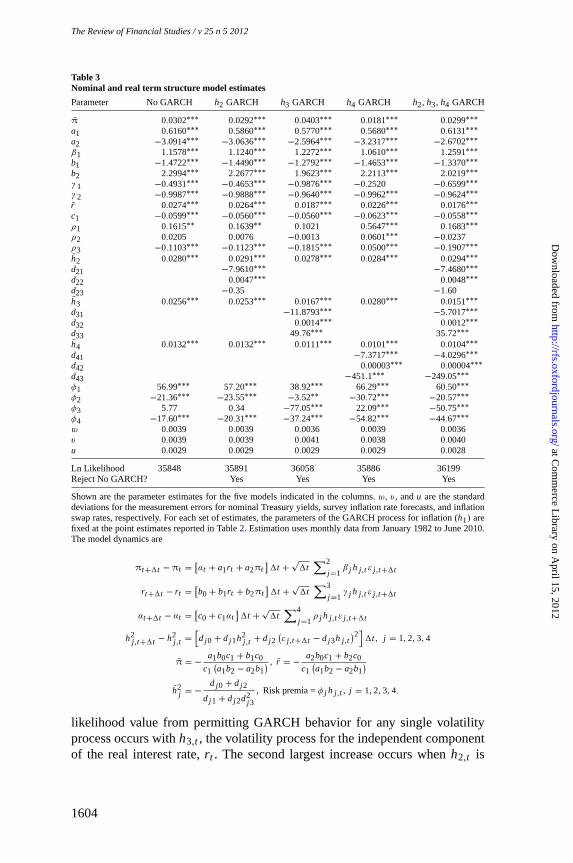
Table 3 reports estimates of the model’s other parameters. To gauge thestatistical significance of permitting GARCH behavior, we estimated theunrestricted model as well as restricted models that assume some of thevolatilities are constant, i.e.,h j,t = h j . The first column of Table3 reportsestimates assuming no GARCH behavior (h j,t = h j , for j = 2, 3, and 4),whereas the second, third, and fourth columns assume GARCH behavior onlyfor h2,t , h3,t , or h4,t , respectively. Finally, the last column of Table3 is theunrestricted model that permits GARCH behavior forh2,t , h3,t , andh4,t .

Inspectionof the log likelihood values for the different models at the bottomof Table 3 indicates that one can reject at the 1% level of significance thehypothesis of no GARCH behavior for each of the less restricted cases.Relative to the model with no GARCH behavior, the largest increase in

Table 2Inflation process estimates

Parameter Estimate t-Statistic p-Value

h1 0.0088 6.12 0.000d11 −2.2034 −2.72 0.007d12 1.88×10−4 3.67 0.000d13 2.54 0.159 0.874

Estimationuses monthly data on inflation and the Blue Chip Economic Indicator one-month survey forecastof inflation from January 1982 to June 2010. The total number of observations is 341. The inflation processdynamics are

It+1tIt

= eπt 1t− 1

2 h21,t 1t + h1,t

√1tε1,t+1t

h21,t+1t − h2

1,t =[d10 + d11h2

1,t + d12(ε1,t+1t − d13h1,t

)2]1t

h21 = −

d10 + d12

d11 + d12d213

.

17 Jarrow and Yildirim (2003) obtain a comparable inflation volatility estimate of 87 basis points.

18 Theprocess displays mean-reversion since the estimate ofd11 is significantly different from the random walkvalue of−1/Δt = −12.

1603

at Com

merce L



ownloaded from



Table 3Nominal and real term structure model estimates

Parameter No GARCH h2 GARCH h3 GARCH h4 GARCH h2, h3, h4 GARCH

π 0.0302∗∗∗ 0.0292∗∗∗ 0.0403∗∗∗ 0.0181∗∗∗ 0.0299∗∗∗

a1 0.6160∗∗∗ 0.5860∗∗∗ 0.5770∗∗∗ 0.5680∗∗∗ 0.6131∗∗∗

a2 −3.0914∗∗∗ −3.0636∗∗∗ −2.5964∗∗∗ −3.2317∗∗∗ −2.6702∗∗∗

β1 1.1578∗∗∗ 1.1240∗∗∗ 1.2272∗∗∗ 1.0610∗∗∗ 1.2591∗∗∗

b1 −1.4722∗∗∗ −1.4490∗∗∗ −1.2792∗∗∗ −1.4653∗∗∗ −1.3370∗∗∗

b2 2.2994∗∗∗ 2.2677∗∗∗ 1.9623∗∗∗ 2.2113∗∗∗ 2.0219∗∗∗

γ 1 −0.4931∗∗∗ −0.4653∗∗∗ −0.9876∗∗∗ −0.2520 −0.6599∗∗∗

γ 2 −0.9987∗∗∗ −0.9888∗∗∗ −0.9640∗∗∗ −0.9962∗∗∗ −0.9624∗∗∗

r 0.0274∗∗∗ 0.0264∗∗∗ 0.0187∗∗∗ 0.0226∗∗∗ 0.0176∗∗∗

c1 −0.0599∗∗∗ −0.0560∗∗∗ −0.0560∗∗∗ −0.0623∗∗∗ −0.0558∗∗∗

ρ1 0.1615∗∗ 0.1639∗∗ 0.1021 0.5647∗∗∗ 0.1683∗∗∗

ρ2 0.0205 0.0076 −0.0013 0.0601∗∗∗ −0.0237ρ3 −0.1103∗∗∗ −0.1123∗∗∗ −0.1815∗∗∗ 0.0500∗∗∗ −0.1907∗∗∗

h2 0.0280∗∗∗ 0.0291∗∗∗ 0.0278∗∗∗ 0.0284∗∗∗ 0.0294∗∗∗

d21 −7.9610∗∗∗ −7.4680∗∗∗

d22 0.0047∗∗∗ 0.0048∗∗∗

d23 −0.35 −1.60h3 0.0256∗∗∗ 0.0253∗∗∗ 0.0167∗∗∗ 0.0280∗∗∗ 0.0151∗∗∗

d31 −11.8793∗∗∗ −5.7017∗∗∗

d32 0.0014∗∗∗ 0.0012∗∗∗

d33 49.76∗∗∗ 35.72∗∗∗

h4 0.0132∗∗∗ 0.0132∗∗∗ 0.0111∗∗∗ 0.0101∗∗∗ 0.0104∗∗∗

d41 −7.3717∗∗∗ −4.0296∗∗∗

d42 0.00003∗∗∗ 0.00004∗∗∗

d43 −451.1∗∗∗ −249.05∗∗∗

φ1 56.99∗∗∗ 57.20∗∗∗ 38.92∗∗∗ 66.29∗∗∗ 60.50∗∗∗

φ2 −21.36∗∗∗ −23.55∗∗∗ −3.52∗∗ −30.72∗∗∗ −20.57∗∗∗

φ3 5.77 0.34 −77.05∗∗∗ 22.09∗∗∗ −50.75∗∗∗

φ4 −17.60∗∗∗ −20.31∗∗∗ −37.24∗∗∗ −54.82∗∗∗ −44.67∗∗∗

w 0.0039 0.0039 0.0036 0.0039 0.0036v 0.0039 0.0039 0.0041 0.0038 0.0040u 0.0029 0.0029 0.0029 0.0029 0.0028

Ln Likelihood 35848 35891 36058 35886 36199Reject No GARCH? Yes Yes Yes Yes

Shown are the parameter estimates for the five models indicated in the columns.w, v, andu arethe standarddeviations for the measurement errors for nominal Treasury yields, survey inflation rate forecasts, and inflationswap rates, respectively. For each set of estimates, the parameters of the GARCH process for inflation (h1) arefixed at the point estimates reported in Table2. Estimation uses monthly data from January 1982 to June 2010.The model dynamics are

πt+1t −πt =[αt + a1rt + a2πt

]1t +

√1t

∑2

j =1β j h j,t ε j,t+1t

rt+1t − rt =[b0 + b1rt + b2πt

]1t +

√1t

∑3

j =1γ j h j,t ε j,t+1t

αt+1t − αt =[c0 + c1αt

]1t +

√1t

∑4

j =1ρ j h j,t ε j,t+1t

h2j,t+1t − h2

j,t =[dj 0 + dj 1h2

j,t + dj 2(ε j,t+1t − dj 3h j,t

)2]1t, j = 1,2,3,4

π = −a1b0c1 + b1c0

c1(a1b2 − a2b1

) , r = −a2b0c1 + b2c0

c1(a1b2 − a2b1

)

h2j = −

dj 0 + dj 2

dj 1 + dj 2d2j 3

, Riskpremia =φ j h j,t , j = 1,2,3,4.

likelihood value from permitting GARCH behavior for any single volatilityprocess occurs withh3,t , the volatility process for the independent componentof the real interest rate,rt . The second largest increase occurs whenh2,t is

1604

at Com

merce L



ownloaded from



able to display GARCH, which is the independent volatility component forexpected inflation,πt . Allowing for GARCH effects is least important forh4,t ,theindependent volatility component of the central tendency. The last columnof Table 3 indicates that for the fully unrestricted case in whichh2,t , h3,t ,andh4,t all follow GARCH processes, all of the GARCH volatility parameters(d22, d32, andd42) are significantly positive. Based on these unrestricted modelestimates and those for the inflation GARCH process in Table2, measures ofpersistence forh2

j,t , j = 1, . . . , 4, can be computed. The half-life for a shockin h2

j,t to revert to its steady stateof h2j is 3.4 months, 0.7 months, 1.6 months,

and 4.6 months forj = 1, 2, 3, and 4, respectively.19

3.2 Levels of state variablesWe obtain reasonable estimates for the unconditional means of inflation and thereal interest rate. The unrestricted model estimateof π is 2.99%, just below thesample average BCEI one-month inflation forecast of 3.05% shown in Table1.This estimate, along with the estimated steady-state one-month real rateof

r = 1.76%,and the estimated steady-state inflation risk premium of−φ1h21 =

−0.47%, imply from Equation (5) that the steady-state one-month nominal

interest rateis i = r +π−φ1h21 = 4.28%,somewhat below the sample average

one-month Treasury bill rate of 4.75% given in Table1. Table3 also shows thatpermitting a central tendency for inflation is important since the mean reversionparameter estimate ofc1 is −0.056and is significantly different from both zeroand the no-central-tendency case ofc1 = −1/Δt = −12.

Figure 2 plots the model-implied state variables over the 1982-to-2010sample period. The top panel indicates that the rate of expected inflation overone month,πt , trended downward since the early 1980s. At the beginning, thecentral tendency for inflation was aboveπt , as investors apparently thoughtlonger-term inflation would remain high. However, the Federal Reserve mayhave gained credibility in lowering inflation since the central tendency laterdeclined to the short-run expected inflation rate. Early in 2008, expectedinflation rose significantly and then plunged at mid-year as the financial crisisworsened.

The bottom panel in Figure2 displays the one-month real interest rate,rt . There was an unusually long period from mid-2002 to 2005 when it wasnegative, consistent with the belief that real rates were kept too low for too longand inflated a credit bubble.20 Thepanel also shows that at the start of 2008, theone-month real rate was negative and then rose dramatically, consistent withthe opposite movement in expected inflation as the nominal rate remained near

19 Thehalf-life in periods of lengthΔt (months)is ln( 1

2)/ ln

(1 +

(dj 1 + dj 2d2

j 3

)Δt).

20 During this period, as well as the brief period in 1994 when the real rate was negative, the Federal Reservepegged the federal funds rate below the rate recommended by the Taylor rule.

1605

at Com

merce L



ownloaded from



Figure 2Levels of state variablesThe top figure shows the time series of one-month expected inflation and inflation’s central tendency, and thebottom figure gives the one-month real interest rate. The time series covers the January 1982 to May 2010 sampleperiod.

zero during this time. At the end of 2009, the real rate became negative again,consistent with the Federal Reserve’s pegging of short-term nominal rates nearzero.

Our model estimates of these state variables’ processes indicate relativelystrong mean-reversion for expected inflation and real rates but high persistencefor inflation’s central tendency. The half-lives for the variables to return totheir steady states following a deviation are 0.26, 0.65, and 12.38 years forπt ,rt , andαt , respectively. That inflation’s central tendency displays very weakmean-reversion suggests that investors’ long-run inflation expectations are notwell anchored.

3.3 State variable volatilities and correlationsBased on the unrestricted model’s parameter estimates, Table4 reports statis-tics for the implied standard deviations and correlations for inflation, expectedinflation, the real rate, and the central tendency. The first column calculatesthe state variables’ annualized standard deviations and correlations over a one-month horizon, assuming that each of the GARCH processes begins at theirsteady-state values:h j,t = h j , j = 1, . . . ,4. The real interest rate,rt , and

1606

at Com

merce L



ownloaded from



Table 4Time variation of standard deviations and correlations

1982 to 2010 Sample PeriodSteady State Average Minimum Maximum

StandardDeviationsln(It+1t /It ) 0.0088 0.0083 0.0039 0.0210πt+1t 0.0314 0.0294 0.0166 0.0919rt+1t 0.0326 0.0344 0.0173 0.0886αt+1t 0.0109 0.0113 0.0077 0.0170

Correlationsln(It+1t /It ), πt+1t 0.354 0.371 0.133 0.729ln(It+1t /It ), rt+1t −0.179 −0.167 −0.406 −0.051ln(It+1t /It ), αt+1t 0.136 0.126 0.050 0.289πt+1t , rt+1t −0.874 −0.773 −0.990 −0.285πt+1t , αt+1t −0.011 −0.005 −0.167 0.142rt+1t , αt+1t −0.092 −0.187 −0.687 0.148

The annualized standard deviations and correlations are for one-month horizons and based on parameterestimates from the unrestricted model. The data are monthly over the period January 1982 to June 2010.

expected inflation,πt , have the highest unconditional standard deviations of3.26% and 3.14%, respectively. Conditional on its mean ofπt , the steady-stateone-month standard deviation of log inflation is 0.88%, whereas the steady-state standard deviation of the central tendency is 1.09%. One also sees that aninnovation in actual inflation (It+Δt ) has a 0.35 correlation with an innovationin expected inflation (πt+Δt ) and a 0.13 correlation with an innovation in thecentral tendency (αt ). This suggests that when investors experience a positiveinflation surprise, their one-month expectation of inflation is partially updatedand, to a lesser degree, so is their longer-horizon expectation of inflation viathe central tendency.

We also see that at the steady state, the one-month expected inflation andreal rate are strongly negatively correlated at−0.87. This is consistent withBenninga and Protopapadakis(1983),Summers(1983), andPennacchi(1991)and is likely a consequence of Federal Reserve policy that keeps short-termnominal rates stable by pegging the federal funds rate. Controlling the short-run nominal rate implies that any change in short-run inflation expectationsmust lead to an offsetting change in the short-run real rate. Evidence byAng,Bekaert, and Wei(2007) confirms that the short-term real rate is quite variable.

Of course, because of GARCH behavior, the state variables’ standarddeviations and correlations are not constant. Columns 2, 3, and 4 of Table4calculate the model-implied average, minimum, and maximum of the standarddeviations and correlations over the sample period. From the minimum andmaximum values, we see that standard deviations and correlations variedsignificantly. The central tendency’s correlation with real rates and expectedinflation even changed signs. The standard deviations of expected inflation andthe real rate were especially high during the early 1980s, when the FederalReserve was battling to lower inflation expectations, and also during the late2000s, when commodity price volatility picked up and the financial crisis hit.

1607

at Com

merce L



ownloaded from



3.4 The model’s fit to the data3.4.1 Nominal yields. Over our 1982-to-2010 sample period, the averagenominal yield measurement errors (difference between the observed datayields and the model-implied yields) across all maturities is less than threebasis points, with the largest errors occurring early in the period during atime of extreme interest rate volatility. Indeed, the mean error from 1990 to2010 is less than one basis point. As reported in the last column of Table3,the estimated standard deviation of measurement errors for nominal yields isw = 36 basis points, close to the average standard deviation of errors across allmaturities over the sample period of 33.5 basis points. The ten-year maturityhas a standard deviation of 27 basis points. The largest standard deviation oferrors is for the three-month rate (42 basis points).

Compared to other studies that fit both nominal and real term structures, ourresults are satisfactory. For example,Chen, Liu, and Cheng(2010) estimatea multifactor Cox, Ingersoll, and Ross(1985) model using both nominalTreasury and TIPS data and for nominal yields obtain an average measurementerror of 24 basis points and an average measurement error standard deviationof 74 basis points.Christensen, Lopez, and Rudebusch(2010) fit a multifactorGaussian model to nominal and TIPS yields, finding measurement errorsfor ten-year nominal yields to average ten basis points and have a standarddeviation of 11 basis points.

3.4.2 Inflation swap rates. For an inflation swap of a given maturity, theaverage measurement error over the sample is close to zero, with the possibleexception of the 15-year inflation swap, which has a bias of 11 basis points.The sample standard deviation of errors for a given maturity is typically closeto theu = 28 basis point estimate reported in the last column of Table3.

Examining the average measurement errors across maturities at eachmonthly date during our sample, the errors stay within a band of 50 basis pointsfrom zero, except during November 2008, when the errors exceed 100 basispoints. Whereas during the financial crisis our model over predicted actualinflation swap rates, recall from Figure1 that TIPS break-even inflation rateswere even smaller than were swap rates at that time. Thus, had we used TIPS inour model estimation, measurement errors would likely have been much larger.Indeed, in fitting their model to TIPS,Christensen, Lopez, and Rudebusch(2010) obtained huge measurement errors during this period.

3.4.3 Survey forecasts of inflation. Examining the difference betweenactual and model-implied survey forecasts of inflation, on average the modelover predicts two- and three-quarter BCEI inflation forecasts by less than sevenbasis points but under predicts seven- and eight-quarter inflation forecastsby around six and nine basis points, respectively. The bias for the ten-yearSPF forecast is less than one basis point. The sample standard deviations

1608

at Com

merce L



ownloaded from


Inflation Expectations, Real Rates, and Risk Premia: Evidence from Inflation Swaps

of measurement errors across maturities range from 48 to 36 basis points,consistent with thev = 40 basis point standard deviation estimate reportedin the last column of Table3.

By calculating the average measurement error across all forecast maturitiesfor each monthly date, we find that the model tended to under predict surveyforecasts during the late 1980s and over predict during the late 1990s. Duringmost of the recent financial crisis, the model under predicted expected inflationrelative to the survey forecasts. Recall that during this same time the model wasover predicting inflation swap rates. Hence, during the crisis the model wasmaking a compromise between the relatively high survey inflation expectationsand the relatively low inflation expectations reflected in swap rates.

3.5 Nominal bond yields, risk premia, and volatilityThis section investigates the model-implied term structure of nominal yields,nominal bonds’ risk premia, and the volatility of nominal yields. Figure3shows the model’s nominal yield curve (solid line) when all variables equaltheir steady states. Yields appear reasonable, even for maturities out to 30years, a horizon in which no Treasury data were used. The slopes of this steady-state nominal yield curve (difference between yields and the steady-stateone-month nominal rate ofi = 4.28%) equal 114, 177, 236, and 257 basispoints at the five-, ten-, 20-, and 30-year maturities, respectively. Moving from

Figure 3Steady-state yield curves and expected excess returnsThe graph shows the nominal and inflation-indexed (real) yield curves when all state variables are at theirsteady-states. Also shown are the expected excess nominal returns on nominal bonds and the expected excessreal returns on real bonds (expected returns relative to one-month maturity return).

1609

at Com

merce L



ownloaded from



this steady-state yield curve, let us now consider the time-series properties ofyields.

Time-series Properties: Campbell-Shiller Tests and Bond Risk PremiaNote that rates of return onn-period bonds are given by

r (n)j,t+ΔtΔt = ln

(P(n−1)

j,t+Δt/P(n)j,t

)= y(n)

j,t (nΔt)

− y(n−1)j,t+Δt (n − 1)Δt, for j = N, R, (24)

where if j = N (j = R), Equation (24) denotes the nominal (real) rate of returnon a nominal (real) bond. Sincey(1)

N,t = i t andy(1)R,t = rt , Equation (24) implies

that the corresponding expected excess returns (risk premia) equal

π(n)j,t = Et

[r (n)

j,t+Δt

]− y(1)

j,t , for j = N, R

=(

y(n)j,t − Et

[y(n−1)

j,t+Δt )])

(n − 1) + s(n)j,t , (25)

wheres(n)j,t = y(n)

j,t − y(1)j,t is the slope of the yield curve. The Appendix shows

that these return risk premia,π(n)j,t , for our model are linear functions only of the

four volatility-state variables,h2j,t , j = 1, . . . , 4. Figure3 shows that if these

state variables equal their steady states (h2j,t = h

2j ), then both nominal and real

risk premia are concave functions of maturity (dotted and short-dashed lines).Many empirical studies, notablyFama and Bliss(1987) andCampbell andShiller (1991), provide overwhelming evidence of significant time variation innominal bond risk premia. We now consider whether our model fits the patternsdocumented by prior empirical research. Equation (25) can be rearranged as

Et (y(n−1)j,t+Δt ) − y(n)

j,t =s(n)

j,t

n − 1−π

(n)j,t

n − 1, j = N, R. (26)

Basedon this equation, consider the following regression:

y(n−1)j,t+Δt − y(n)

j,t = β(n)j,0 + β

(n)j,1

s(n)j,t

n − 1+ β

(n)j,2

π(n)j,t

n − 1+ ε

(n)j,t+Δt , j = N, R. (27)

For nominal yields (j = N), Campbell and Shiller(1991) examined the“Expectations Hypothesis” by settingβ(n)

N,2 = 0 and testing ifβ(n)N,1 = 1.

Theirtests rejected this hypothesis, and estimates forβ(n)N,1 becameincreasingly

negative as maturity,n, increased. Allowingβ(n)N,2 to be unconstrained and

using a three-factor Gaussian model with the “essentially affine” risk premiumstructure ofDuffee(2002), empirical tests byDai and Singleton(2000) couldnot reject the hypothesis thatβ

(n)N,1 = 1 andβ

(n)N,2 = −1.

1610

at Com

merce L



ownloaded from



We repeat the Campbell-Shiller regressions (β(n)N,2 constrainedto zero) using

actual monthly nominal Treasury yields for our 1982-to-2010 sample period,and estimates of the slope coefficientβ

(n)N,1 areshown in the first column of

Table 5. The null hypothesis thatβ(n)N,1 = 1 is rejected for all maturities at

Table 5Campbell-Shiller regressions for nominal yields

Actual Model-Implied

Expectations Including Model Expectations Including ModelHypothesis Risk Premium Hypothesis Risk Premium

Maturity Risk Joint Test Risk Joint Test(Years) Slope p−Value Slope Premium p−Value Slope p−Value Slope Premium p−Value

0.02 0.77 −0.86 0.07 2.53 −1.561 (0.28) 0.00 (0.31) (0.18) 0.67 (0.41) 0.02 (0.55) (0.25) 0.02

−3.54 −0.72 0.81 −2.28 2.77 −2.24

−0.15 0.90 −1.12 0.04 1.71 −1.482 (0.51) 0.03 (0.58) (0.30) 0.84 (0.52) 0.06 (0.60) (0.29) 0.24

−2.24 −0.17 −0.39 −1.86 1.19 −1.65

−0.45 0.70 −1.38 −0.34 0.93 −1.513 (0.71) 0.04 (0.80) (0.47) 0.73 (0.66) 0.05 (0.75) (0.44) 0.39

−2.04 −0.38 −0.81 −2.01 −0.09 −1.16

−1.21 −0.12 −1.69 −1.41 −0.64 −1.355 (1.04) 0.03 (1.11) (0.97) 0.24 (1.06) 0.02 (1.22) (1.05) 0.21

−2.12 −1.01 −0.71 −2.27 −1.35 −0.34

−1.93 −1.32 −0.48 −2.48 −2.34 −0.307 (1.35) 0.03 (1.32) (1.22) 0.20 (1.50) 0.02 (1.64) (1.46) 0.12

−2.17 −1.76 0.42 −2.32 −2.03 0.48

−2.80 −2.03 0.54 −3.82 −3.86 0.0810 (1.80) 0.04 (1.59) (1.03) 0.08 (2.15) 0.03 (2.21) (1.30) 0.09

−2.11 −1.91 1.50 −2.25 −2.19 0.84

−3.71 −2.22 0.75 −5.30 −5.28 −0.0515 (2.52) 0.06 (2.08) 0.86 0.05 (3.12) 0.04 (3.16) (1.13) 0.12

−1.87 −1.55 −2.05 −2.02 −1.99 0.84

Theleft panel shows the results for Campbell-Shiller regressions of the monthly changes in actual nominal yieldsagainst the adjusted slope (slope divided by maturity in months minus 1) over the period January 1982 to May2010:

y(n−1)N,t+1t − y(n)

N,t = β(n)N,0 + β

(n)N,1

s(n)N,t

n − 1+ ε

(n)N,t+1t .

For each maturity (in years), the coefficients of the adjusted slope are shown together with the standard error and

thet-statisticfor the null hypothesis thatβ(n)N,1 = 1. The column next to the slope column reports thep-value for

the testβ(n)N,1 = 1. The next two columns report the results for regressions that include the model-implied time

varying risk premium:

y(n−1)N,t+1t − y(n)

N,t = β(n)N,0 + β

(n)N,1

s(n)N,t

n − 1+ β

(n)N,2

π(n)N,t

n − 1+ ε

(n)N,t+1t .

For each maturity, the coefficients of the adjusted slope are shown together with the standard error and the

t-statisticfor the null hypothesis thatβ(n)N,1 = 1. The coefficients of the adjusted risk premium are shown together

with the standard error and thet-statisticfor the null hypothesis thatβ(n)N,2 = −1.The p-value is now for the joint

test thatβ(n)N,1 = 1 andβ

(n)N,2 = −1. Theright panel repeats the tests using the model-implied nominal yields.

1611

at Com

merce L



ownloaded from



the 10% significance level, and estimates become more negative as maturityincreases. The second column of the table reports results of regression (27)with our model-implied risk premia,π(n)

N,t , computed at each date. There, onesees that the joint hypothesis that the slope is 1 and the excess return coefficientis −1 cannot be rejected at the 10% significance level, except for the ten- and15-year maturities. In these regressions, the dependent variable and slope arefrom actual Treasury yields. Replacing them by model-implied yields for eachdate from 1982 to 2010, similar results are obtained, as shown in the right-mostpanel of Table5.

Thus, our model generates time-varying risk premia that are, for mostmaturities, not inconsistent with the theoretical relation (26). The variation canbe substantial. Excess expected returns on longer-dated bonds became negativeseveral times, almost always during episodes of financial market turmoil:May to December 1982 (Paul Volker’s Federal Reserve sharp tightening ofmonetary policy); November to December 1987 (stock market crash); June toAugust 1997 (Asian financial crisis); October 1998 (Russian financial crisis);June to July 2000 (bursting of dot.com bubble); October and November 2001(September 11 terrorist attack); November 2007 to April 2008 (worseningof the subprime crisis); and October 2008 to April 2009 (period followingLehman Brothers’ bankruptcy). That the model predicts negative risk premiaduring financial crises may be reassuring. There is consensus that investorsview Treasury bonds as a “safe haven” during a crisis and bid up their prices,thereby reducing excess expected returns.

Whereas our model’s risk premia are entirely determined by the volatilityfactors (h2

j,t , j = 1, . . . , 4), Figure4 shows that they play a minor role indetermining the cross-section of yields. The figure illustrates the contributionof each of the seven state variables to the six-month, two-year, five-year,and ten-year yields. Since the four volatility-state variables add minimally tothe yields, their collective contribution is shown. Nominal yields are largelydetermined by expected inflation,πt , the real rate,rt , and the central tendency,αt , with the importance of the last state variable increasing as maturityincreases. Only occasionally do the volatility-state variables play a significantrole, and then only for shorter maturities. Our model’s results align withDuffee (2011), who constructs a multifactor Gaussian model in which a subsetof factors describe bond yields and a mutually exclusive subset of “hiddenfactors” determine bond risk premia.

Volatility EffectsUnlike Gaussian models, our model also captures the empirical property thatyields have stochastic volatilities that are weakly linked to yield levels. TheAppendix shows that the covariance of yields are linear functions solely ofthe four volatility-state variables,h2

j,t , j = 1, . . . , 4. When these volatilityvariables are at their steady states, the volatility of nominal yields (annualized

1612

at Com

merce L



ownloaded from



Figure 4Decomposition of nominal yieldsThe panels show the contributions of the one-month expected inflation (πt ), the one-month real rate (rt ), thecentral tendency of inflation (αt ), and the volatility-state variables (h j,t , j = 1, . . . ,4) to the six-month, two-year, five-year, and ten-year maturity nominal yields.

standard deviation of monthly changes) is at a minimum at the two-yearmaturity of just under 1%, rises to a maximum of 1.2% at the eight-yearmaturity, and then falls again to less than 1% at the 20-year maturity. Thetop left panel of Figure5 displays the term structures of yield volatilities overour sample, indicating significant variation at the short end, during the early1980s and early 1990s. The bottom left panel is a scatterplot of the volatilityof the five-year maturity nominal yield against the yield’s level. It indicates apositive relation, with the slope of the regression line being different from zeroat the 1% significance level.

Also in contrast to Gaussian models, our model’s yield changes displayexcess kurtosis and skewness, with changes in yields of one-year maturityand less tending to display negative skewness, whereas longer-maturity yieldchanges are positively skewed.21 Correlations between yields are also time-varying. For example, over our sample period the model-implied correlationbetween one-month changes in the one- and ten-year yields averages 0.37 butreaches a maximum and minimum of 0.67 and−0.05, respectively.

Collectively, then, whereas completely affine, our model captures thetime-series properties of nominal yields fairly well. Given its reasonable

21 For example, average sample skewness for a one-year change in the three-month and ten-year yields is−0.43and 0.46, respectively.

1613

at Com

merce L



ownloaded from



Figure 5Volatility of nominal and real yieldsPanel A shows the time series of nominal yield curve volatilities and real yield volatilities at monthly intervalsover the 1982-to-2010 sample period. Over this same period, the left figure in Panel B plots the five-year nominalyield versus the five-year nominal yield volatility, whereas the right figure in Panel B plots the five-year realyield versus the five-year real yield volatility. Both figures in Panel B show regression lines, whose slopes arestatistically different from zero at the 1% confidence level.

performance for describing nominal yields, we next consider their decomposi-tion into real and inflation components.

3.6 Real bond yields, risk premia, and volatilityFigure3 shows the model-implied inflation-indexed (real) yield curve whenall variables equal their steady states (long dashed line). The slopes of this realyield curve (difference between yields and the steady-state one-month real rateof r = 1.76%) equal 52, 96, 149, and 177 basis points at the five-, ten-, 20-,and 30-year maturities, respectively. Similar to the steady-state nominal yieldcurve, this real yield curve is concave and upward sloping but less steep. PanelA of Figure 6 shows much time-series variation in the term structure of realyields over the 1982-to-2010 sample period, particularly at short maturities.

Since Equation (26) holds both in real and nominal terms, regression (27)relating yields to term structure slopes and risk premia should also hold forreal yields withβ

(n)R,1 = 1 andβ

(n)R,2 = −1. Being unaware of prior research

examining regression (27) for real rates, we carried out such a test of our modelover two different sample periods. First, during 2003 to 2010 when inflationswap data are available, Equation (16) was used to obtain “actual” zero-coupon

1614

at Com

merce L



ownloaded from



Figure 6Term structures of real yields and inflation expectationsThe top figure shows the model-implied time series of the term structure of real (inflation-indexed) yields overthe 1982-to-2010 sample period. The bottom figure shows the model-implied time series of the term structure ofexpected inflation over the same period.

real yields,y(n)R,t , by subtracting the inflation swap rate from the equivalent

maturity nominal Treasury yield. From these real yields, slope variables,s(n)R,t ,

were calculated. Second, over the entire 1982-to-2010 period, we calculated

1615

at Com

merce L



ownloaded from



model-impliedslopess(n)R,t from the model-implied real yields (as shown in

Panel A of Figure6). For both the first and second samples, the model-impliedreal risk premia,π(n)

R,t , were calculated from the time series of the volatility-state variables.

Table 6 reports results of regression (27) both with the risk premiumcoefficientβ(n)

R,2 restrictedto zero (Expectations Hypothesis) and unrestricted.

Table 6Campbell-Shiller regressions for real yields

Actual Model-Implied

Expectations Including Model Expectations Including ModelHypothesis Risk Premium Hypothesis Risk Premium

Maturity Risk Joint Test Risk Joint Test(Years) Slope p-Value Slope Premium p−Value Slope p−Value Slope Premium p−Value

0.21 0.15 0.31 1.91 2.64 −1.262 (0.77) 0.31 (0.81) (1.19) 0.41 (0.35) 0.01 (0.38) (0.28) 0.00

−1.03 −1.05 1.10 2.59 4.32 −0.92

0.58 0.66 −0.38 1.60 2.28 −1.423 (0.88) 0.64 (0.93) (1.46) 0.89 (0.37) 0.10 (0.39) (0.33) 0.00

−0.47 −0.37 0.42 1.65 3.30 −1.26

1.00 1.55 −2.19 1.14 1.96 −2.045 (1.05) 1.00 (1.17) (2.03) 0.82 (0.48) 0.78 (0.53) (0.59) 0.11

0.00 0.47 −0.59 0.28 1.80 −1.79

1.64 2.99 −4.36 0.78 1.80 −2.767 (1.36) 0.64 (1.58) (2.63) 0.35 (0.65) 0.73 (0.74) (0.97) 0.19

0.47 1.26 −1.28 −0.34 1.08 −1.82

2.09 4.70 −6.95 0.36 1.19 −2.3510 (1.72) 0.53 (1.98) (2.87) 0.09 (0.91) 0.48 (1.01) (1.24) 0.53

0.63 1.86 −2.07 −0.70 0.19 −1.09

2.28 5.58 −7.18 −0.10 0.37 −1.2915 (2.48) 0.61 (2.86) (3.31) 0.14 (1.32) 0.40 (1.38) (1.15) 0.83

0.51 1.60 −1.87 −0.84 −0.46 −0.25

The left panel shows the results for Campbell–Shiller regressions of the monthly changes in actual real yieldsagainst the adjusted slope (slope divided by maturity in months minus 1) over the period January 2003 to May2010:

y(n−1)R,t+1t − y(n)

R,t = β(n)R,0 + β

(n)R,1

s(n)R,t

n − 1+ ε

(n)R,t+1t .

Realyields in this panel were derived as the difference between the equivalent maturity nominal Treasury yieldand the inflation swap rate. For each maturity, the coefficients of the adjusted slope are shown together with the

standard error and thet-statisticfor the null hypothesis thatβ(n)R,1 = 1. The column next to the slope column

reports thep-value for the testβ(n)R,1 = 1.

The next two columns report the results for regressions that include the model-implied time-varying riskpremium:

y(n−1)R,t+1t − y(n)

R,t = β(n)R,0 + β

(n)R,1

s(n)R,t

n − 1+ β

(n)R,2

π(n)R,t

n − 1+ ε

(n)R,t+1t .

For each maturity, the coefficients of the adjusted slope are shown together with the standard error and the

t-statisticfor the null hypothesis thatβ(n)R,1 = 1. The coefficients of the adjusted risk premium are shown together

with the standard error and thet-statisticfor the null hypothesis thatβ(n)R,2 = −1. The p-value is now for the

joint test thatβ(n)R,1 = 1 andβ

(n)R,2 = −1. Theright panel repeats the tests using the model-implied real yields.

1616

at Com

merce L



ownloaded from



Interestingly, there are qualitative differences compared to the nominal resultsof Table 5. Using the “actual” real rates from 2003 to 2010, the left panelreports that the regression, including only the slope term, does not reject thehypothesisβ(n)

R,1 = 1. Unlike the nominal results, the estimatesβ(n)R,1 become

more positive as maturity increases. When the real risk premium,π(n)R,t , is

included in the regression, rejection of the joint hypothesis ofβ(n)R,1 = 1 and

β(n)R,2 = −1 at a 10% level of significance occurs only for the ten-year maturity,

but this happens becauseβ(n)R,1 becomestoo positive, whereasβ(n)

R,2 becomestoonegative, just the opposite of the nominal regressions where rejection occurredbecauseβ(n)

R,1 becamenegative, whereasβ(n)R,2 becamepositive.

These findings could be partly due to the short 2003-to-2010 sample. Whenin the right panel of Table6 we use the model-implied real yields from 1982to 2010, the estimate ofβ(n)

R,1 doesdecline when the slope alone is included inthe regression. However, except for the 15-year maturity, the estimated slopecoefficient is positive, and the hypothesis thatβ

(n)R,1 = 1 cannot be rejected.

Notably, when the real risk premium,π(n)R,t , is included, the model fits well

at the longer maturities but is rejected at the shorter ones. Again, however,rejection at short maturities occurs becauseβ

(n)R,1 exceeds 1, whereasβ(n)

R,2 islower than−1.

Volatility EffectsIt is apparent from the top panel of Figure6 that short-maturity real yieldstend to be more volatile than longer-maturity ones, consistent with the topright panel of Figure5 that shows the term structures of real yield volatilitiesover our sample period.22 Thebottom right panel in Figure5 displays a scatterdiagram of the levels of five-year real yields versus their volatilities over oursample period and indicates, like nominal yields, a positive relation betweenyields’ levels and their volatility. The slope of the regression line is statisticallydifferent from zero at the 1% level of significance.

The high volatility of short-term real yields is consistent with Figure2’sreported high standard deviation of the one-month real rate,rt . Since theFederal Reserve’s policy pegs short-term nominal rates, changes in short-runinflation expectations induce almost opposite changes in short-run real yields.

3.7 Expected inflation and inflation and real risk premiaPanel B of Figure6 shows our model’s implied term structures of expectedinflation for each month from 1982 to 2010. Consistent with the evidence inFigure2 of a falling central tendency, inflation expectations trended downward

22 Whenh j,t = h j , j − 1, . . . , 4, the real yield volatilities (annualized standard deviation of monthly changes) are112 basis points at the one-year maturity, falling to 68 basis points at the four-year maturity, rising to 72 basispoints at the eight-year maturity, and gradually falling to 61 basis points at the 20-year maturity.

1617

at Com

merce L



ownloaded from



atall maturities. However, the term structure was often upward sloping duringthe mid-1980s, suggesting that investors were not yet convinced that inflationwould remain low in the longer run. Expected inflation can be volatile at shortmaturities but is smoother at longer horizons.

Other components of nominal yields that interest policymakers and aca-demics are the term structures of inflation and real risk premia. Saving thecost of an inflation risk premium is used to justify a government’s issuanceof inflation-indexed bonds, and this premium must first be quantified to deriveinflation expectations from an inflation swap or TIPS break-even inflation rate.In addition, the term structure of real risk premia provides information on howthe real cost of financing varies by maturity.

We quantify the term structures of inflation and real risk premia in thefollowing manner.23 Considerour model’s nominal and real yield curves whenall of the market prices of risk are set to zero, i.e.,φ ≡ (φ1 φ2 φ3 φ4) = 0.Sinceyields on nominal and inflation-indexed bonds maturing inn periods aredenoted asy(n)

j,t , j = N, R, respectively, let their zero-risk premium counter-

parts bey(n)j,t (φ = 0), j = N, R. Then denote the datet , n-period real and

inflation risk premia asΦ(n)R,t andΦ

(n)inf,t , respectively, with their sum defined as

the nominal risk premium,Φ(n)N,t . These premia are computed as

Φ(n)j,t ≡ y(n)

j,t − y(n)j,t (φ = 0) , j = N, R , (28)

Φ(n)inf,t ≡

(y(n)

N,t − y(n)R,t

)−[y(n)

N,t (φ = 0) − y(n)R,t (φ = 0)

]. (29)

The logic behind definition (29) is that the break-even inflation rate in paren-theses includes expected inflation, the inflation risk premium, and convexityterms unrelated to risk premia. By subtracting the zero-risk premium break-even inflation rate in square brackets, expected inflation and convexity termsare eliminated, leaving only the inflation risk premium. From inspection of theformulas for nominal and real yields, given in the Appendix, it can be seenthat all of these risk premia are affine functions of only the four volatility-statevariablesh2

j,t , j = 1, . . . , 4.The term structures of nominal, real, and inflation risk premia when the

volatility-state variables are at their steady states are plotted in Figure7. Thereal risk premia equal 54, 102, 170, and 214 basis points at the five-, ten-, 20-,and 30-year maturities, respectively. The inflation risk premia equal 17, 45, 80,

23 Christensen,Lopez, and Rudebusch(2010) define the inflation risk premium asy(n)N,t − y(n)

R,t −1

nΔt ln(E[It+nΔt /It

]), and Chernov and Mueller(forthcoming) andHordahl and Tristani(2007) define it

asy(n)N,t − y(n)

R,t − E[

1nΔt ln

(It+nΔt /It

)]. These definitions neglect convexity effects, and the former one also

introduces a downward bias that increases with maturity since by Jensen’s Inequality,1nΔt ln

(E[It+nΔt /It

])≥

E[

1nΔt ln

(It+nΔt /It

)]. Our approach accounts for convexity effects, is the same asChen, Liu, and Cheng

(2010), and is quantitatively similar to the latter definition for maturities out to ten years.

1618

at Com

merce L



ownloaded from



Figure 7Real and inflation risk premia for steady stateThe figure shows the term structures of the nominal, real, and inflation risk premia when all volatility-statevariables are at their steady states. The nominal risk premium is the sum of the real and inflation risk premia.

and 100 basis points at the five-, ten-, 20-, and 30-year maturities, respectively.These steady-state term structures are very close to the average of the modelestimates for each month over our sample period.

Note that the steady-state inflation risk premia are negative for shortmaturities, reaching a minimum of−20 basis points at a seven-month maturitybefore becoming positive at a 29-month maturity. An explanation is that ourmodel is capturing the relative attractiveness of shorter maturity Treasuries,particularly Treasury bills, because of their high liquidity or “moneyness.”This is plausible since our longer-maturity yield data were constructed byGurkaynak, Sack, and Wright(2007) from off-the-run Treasury notes andbonds, whereas our shorter-maturity data are actual yields of Treasury billsthat trade in more liquid money markets. A negative inflation premium isthe model’s way of adjusting for the greater liquidity at the short end of thenominal yield curve.24

24 Other research recognizes that bill yields are reduced by high liquidity.Campbell, Shiller, and Viceira(2009)add a parameter to their model estimation to “capture the liquidity effects which lower the yields on Treasurybills relative to the longer-term real yield curve.” Also, note that Figure7 indicates a negative real risk premia atvery short maturities, which is due to our real yield curve truly being yields for inflation-indexed bonds having

1619

at Com

merce L



ownloaded from



We next analyze the time variation of inflation and real risk premia andthe volatility factors that drive their movements. Similar to Figure4 thatdisplays the components of nominal yields, Figure8 shows the componentsof real and inflation risk premia for maturities of two, five, and ten years.The left-most panels show the time series of real risk premia which have fivecomponents: a constant and contributions from each of the four volatility-state variables. As might be expected, the main determinant of the two-year real risk premium ish3,t , the volatility factor determined by shocksto the one-month real interest rate,rt . However, for the five- and ten-year maturity real risk premia, the dominating volatility factor becomesh4,t , which is determined by shocks to inflation’s central tendency,αt .This finding—that long-maturity real risk premia increase with longer-runinflation uncertainty—is consistent with research, such asLucas (1973),Fischer(1981),Cuikerman(1982), andFischer(1991), showing that inflationuncertainty can cause resource misallocation that slows real economic growth.Wright (2011) finds that term premia on nominal government bonds declinedmore in countries that reduced inflation uncertainty. Our results suggestthat the decline may be due to a reduction in both real and inflation riskpremia.

The right-most panels of Figure8 show the time series of two-, five-, andten-year inflation risk premia and the contributions of the volatility factors.For none of these inflation risk premia does theh3,t volatility derived from theindependent shock to the short-term real rate,rt , play a significant role. As issensible, the volatility factor determined by shocks to short-term unanticipatedinflation, h1,t , is the primary driver of changes in the two-year inflation riskpremium, with a rise inh1,t reducingthe inflation risk premium.25 Increasesin h2,t andh4,t , which are the volatility factors determined by shocks to one-month expected inflation,πt , and inflation’s central tendency,αt , respectively,play lesser roles in raising the two-year inflation risk premium. It is alsointuitive that, as maturities increase to the five- and ten-year horizons, the roleof h4,t derived from shocks to inflation’s longer-run central tendency becomesdominant. Uncertainty regarding inflation’s central tendency may proxy forthe credibility of monetary policy, suggesting that the longer-run inflation riskpremia are linked to beliefs of central bank behavior. There are, however, a fewstriking instances when theh1,t factor derived from shocks to unanticipatedinflation plays a big role by reducing the inflation risk premium, even for longmaturities. Figure8 shows that these instances often coincide with financial

a three-month indexation lag. Since these bonds lack inflation protection in their last three months, their modelyields reflect a small inflation risk premium.

25 Thisnegative relation betweenh1,t andthe inflation risk premium is consistent with our positive estimate ofφ1

andthe one-month nominal rate relationi t = rt +πt − φ1h21,t .

1620

at Com

merce L



ownloaded from



Figure 8Decomposition of two-, five-, and ten-year real and inflation risk premiaThe left (right) panels show the decomposition of the real (inflation) risk premium into a constant and fourvolatility-state variable components. The first component (proportional toh1) is driven by the unanticipated rateof inflation; the second component (proportional toh2) that adds to the sum is determined by that orthogonalcomponent that affects expected inflation; the third (proportional toh3) is that orthogonal component that affectsthe real rate, while the fourth (proportional toh4) is that orthogonal component affecting inflation’s centraltendency. These four components are labeledh1,h2,h3 and h4, respectively, since they are proportional tothese respective volatility-state variables. All values are in basis points. The total risk premia in all figures areabove the contribution ofh4. The top panels show the decomposition for two-year maturities, the middle panelsshow the five-year maturities, and the bottom panels show the ten-year maturities.

stress so that a “flight-to-quality” attraction for Treasuries is reflected as adecline in the inflation risk premium.26

Our average estimates for inflation risk premia are in the middle rangeof those found by other studies using different data and different sampleperiods.27 However, our estimates’ ranges of variation may be smaller thanmost: Figure8 shows that the two-, five-, and ten-year inflation risk premiadisplay basis point ranges of−80 to 16,−16 to 30, and 25 to 59, respectively.Some studies may find more volatile inflation risk premia because they use

26 Times when the five-year inflation risk premium turned negative include November 2007 to January 2008(subprime crisis) and October 2008 to February 2009 (Lehman bankrutcy). Earlier we noted that the “safehaven” quality of nominal Treasuries reduced their excess return during periods of stress. Thus, this reductionin return typically takes the form of a declining inflation risk premium.

27 Table1 in Chen, Liu, and Cheng(2010) summarizes empirical studies estimating inflation risk premia.

1621

at Com

merce L



ownloaded from



dataon TIPS yields, that arguably incorporate a volatile liquidity premium,or realized macroeconomic quantities that can introduce excess “noise” inmodel-implied yields.Kim (2009) argues that state variables, such as realizedinflation or realized output growth, are unlikely to be spanned by bond returnsand realistically fail to satisfy dynamic term structure models’ no-arbitrageassumptions. As a result, model-implied yields that assume such macro-statevariables may inherit unspanned noise.28

3.8 Comparison to TIPS yieldsIn the spirit of an out-of-sample test, we relate our model’s implied yieldsfor inflation-indexed bonds to the actual yields of TIPS.29 Figure9 comparesfive- and ten-year zero-coupon TIPS yields from Gurkaynak, Sack, and Wright(2008) for the period January 1999 to June 2010 to our model’s impliedfive- and ten-year zero-coupon yields for inflation-indexed bonds. Our model’syields are significantly below TIPS yields from 1999 to 2004 and are veryclose to TIPS yields from 2004 to mid-2008. Starting in mid-2008, the model-implied yields again fall below the yields on TIPS until they converge inlate 2009. Thus, at the beginning of our sample and during the height of thefinancial crisis, our model overprices inflation-indexed bonds relative to TIPS.One interpretation of this comparison is that our model performs poorly invaluing inflation-indexed bonds, except during 2004 to mid-2008 and againstarting at the end of 2009.

However, recall that prior studies, such asSack and Elsasser(2004),Shen(2006), andD’Amico, Kim, and Wei(2008), conclude that TIPS weresignificantly undervalued prior to 2004, and more recently,Campbell, Shiller,and Viceira (2009), Hu and Worah(2009), andChristensen, Lopez, andRudebusch(2010) argue that there was panic selling of TIPS in the latterhalf of 2008 that drove their yields above, and TIPS break-even inflationbelow, reasonable levels. Therefore, a more logical interpretation is that thedifference in the two curves in Figure9 is confirming an erratic liquiditypremium in TIPS. The model’s close fit to TIPS beginning in 2004 might bepartly attributed to the initiation of a U.S. inflation swap market in 2003 thatin normal times allowed dealers to arbitrage significant underpricing of TIPS(Fleckenstein, Longstaff, and Lustig 2010). In summary, the overall evidence

28 For example, two studies that find more volatile inflation risk premia areChernov and Mueller(forthcoming),who use quarterly realized inflation and linearly de-trended per capita GDP growth as macro-state variables, andHordahl and Tristani(2007), who use monthly realized inflation and deviations of industrial production froma quadratic trend as macro-state variables.Hordahl and Tristani(2007) also use euro-denominated inflation-indexed bonds and mention that the negative inflation risk premia that they find during 2001 to 2002 may be dueto the bonds’ higher illiquidity during that period. Similarly,Christensen, Lopez, and Rudebusch(2010) statethat their estimated inflation risk premium may be affected by TIPS’s liquidity premium.

29 Fleckenstein, Longstaff, and Lustig(2010) compare TIPS to a synthetic real bond constructed from nominalTreasuries and inflation swaps. They find, like us, that TIPS were often underpriced. However, their analysis canstart only in July 2004, when inflation swap data became available. Using our model-implied real yields, ouranalysis can begin earlier in January 1999, when TIPS became available.

1622

at Com

merce L



ownloaded from



Figure 9TIPS yields versus model-implied inflation-indexed yieldsThe figures compare the time series of TIPS yields to the model-implied inflation indexed yields from 1999 to2010. The top panel shows the five-year maturity, whereas the bottom panel displays the ten-year maturity.

supports our earlier arguments for using data on inflation swaps and surveyforecasts of inflation, rather than TIPS, to estimate a nominal and real termstructure model.

4. Conclusion

From June 2004 to June 2005, the Federal Reserve raised the target federalfunds rate eight times, from 1.00% to 3.00%. However, during this time longer-term Treasury yields fell, with the ten-year note’s yield declining from 4.69%to 4.00%. Chairman Alan Greenspan testified before the U.S. Congress thatthis pattern presented a “conundrum.” According to our model, this decline inthe ten-year yield can be apportioned almost evenly between reductions in ten-year expected inflation (28 basis points) and the ten-year real yield (27 basispoints), as well as a fall in the 10-year inflation risk premium (12 basis points).The economic intuition from the model is that the Federal Reserve’s tighteningincreased investor confidence in monetary discipline by lowering inflation’s“central tendency.” Moreover, a reduction monetary uncertainty proxied by aless volatile central tendency reduced both real and inflation risk premia.

Our completely affine model of nominal and real term structures differs fromothers by having four sources of uncertainty but seven state variables. The

1623

at Com

merce L



ownloaded from



model’s factors include the short-term real rate, the short-term rate of expectedinflation, and inflation’s central tendency. These factors largely determine thecross-section of bond yields, whereas their innovations, along with innovationin actual inflation, drive four additional volatility-state variables. The volatilityfactors follow the nonlinear asymmetric GARCH model ofEngle and Ng(1993) and exclusively determine bond risk premia that vary over time andcan even change signs. Our study also breaks new ground by estimating themodel using data on nominal yields, and survey forecasts of inflation, and alsoinflation swap rates.

Because of the Federal Reserve’s policy of pegging short-term nominalrates, the short-term real rate is typically highly negatively correlated withchanges in short-run expected inflation. Short-term real rates are quite volatileand were negative from 2002 to 2005, which may have led to an overexpansionof credit. However, inflation’s longer-run central tendency trended downwardover our 1982-to-2010 sample period and continues to be low, despite a re-emergence of negative real rates.

We also find that real risk premia at short maturities increase when thevolatility of the short-term real interest rate is high, but greater longer-maturity real risk premia are generated mainly by greater volatility frominflation’s central tendency, consistent with real costs of longer-run inflationuncertainty. Inflation risk premia at short maturities are inversely related tothe volatility of unanticipated inflation. However, longer-run inflation riskpremia respond positively to greater volatility from inflation’s central tendency.However, during periods of financial crisis, we find that the “flight-to-quality”attraction for longer-run Treasuries can be linked to unexpected deflation thatcan substantially lower nominal bonds’ excess returns via a decline in theirinflation risk premia.

Finally, comparing our model’s implied yields for inflation-indexed bondsto those of TIPS suggests that TIPS bore a large liquidity premium prior to2004. Perhaps because of the 2003 introduction of inflation derivatives, suchas inflation swaps, arbitrage possibilities may have eliminated TIPS mispricinguntil the middle of 2008. However, after the Lehman Brothers’ bankruptcyin September 2008, the link between nominal Treasuries, TIPS, and inflationswaps was broken, and a very large liquidity premium for TIPS reappeared.

Appendix

Proof of Proposition 1The dynamics forπt , rt , andαt arestraightforward. The interesting diffusion limits are for the

h2j,t statevariables. Substitute the expressions fordj,i , i = 0, . . . , 3, given in Proposition 1, into

the last line of Equation (6). Upon simplification, this leads to

Δh j,t = (κ j θ j +1

4υ2

j )Δt +1

4υ2

j (ε2j,t+Δt − 1)Δt + h2

j,tκ jΔt (κ jΔt

4− 1)

−υ j (1 −κ j υ j

2Δt)

√Δth j,t ε j,t+Δt . (A1)

1624

at Com

merce L



ownloaded from



Taking limit of this expression, the second term converges to zero, which leads to the result.

Lemma 1. Let X ∼ N (0,1). Then for Q2 > − 12 , E

[eQ1X−Q2X2

]=

exp

[Q2

12(1+2Q2) − 1

2 ln(1 + 2Q2)

].

Proof:

The expectation can be written asE[eQ1X−Q2X2

]= 1√

2π

∫∞−∞ eQ1x−Q2x2− 1

2 x2dx, and

the result follows after completing the square and using properties of the normal density.

Proof of Proposition 2The proof of the first result follows by substituting the nominal pricing kernel into the bond

pricing equation,P(n)N,t = Et [

Mt+ΔtMt

P(n−1)N,t+Δt ], to obtain

P(n)N,t = Et

[e−(πt +rt −φ1h2

t )Δt− 12∑4

j =1 φ2j h2

j,tΔt−∑4

j =1 φ j h j,t√Δtε j,t+Δt P(n−1)

N,t+Δt

]. (A2)

Now assume the bond price has the form of Equation (18), and substitute it into the left- andright-hand sides of Equation (A2). Substituting in for the state variables at datet + Δt usingEquation (6), collecting all coefficients of the random variables of the same type together, and thentaking expectations using Lemma 1 leads to the resulting recursive equations for the coefficients.The initial boundary conditions come from considering the case in whichn = 1. The recursiveequations are

Kn+1 = Kn + (b0Bn + c0Cn + Σ4j =1dj 0D j,n)Δt

+1

2Σ4

j =1 ln(1 + 2D j,ndj 2Δt)

An+1 = Δt + (1 + a2Δt) An + b2BnΔt

Bn+1 = Δt + a1Δt An + (1 + b1Δt) Bn

Cn+1 = AnΔt + (1 + c1Δt) Cn

D j,n+1 =

−φ1 I{ j =1} +φ2

j

2

Δt + D j,n

(1 +

(dj 1 + dj 2d2

j 3

)Δt)

−Q2

j,n

2(1 + 2D j,ndj 2Δt), (A3)

whereI{ j =1} is the indicator function equal to 1 ifj = 1 and is 0 otherwise, and

Q1,n = (φ1 + Anβ1 + Bnγ1 + Cnρ1 − D1,n2d12d13√Δt)

√Δt

Q2,n = (φ2 + Anβ2 + Bnγ2 + Cnρ2 − D2,n2d22d23√Δt)

√Δt (A4)

Q3,n = (φ3 + Bnγ3 + Cnρ3 − D3,n2d32d33√Δt)

√Δt

Q4,n = (φ4 + Cnρ4 − D4,n2d42d43√Δt)

√Δt .

Next consider the pricing of TIPS. Lett be the current date,te = t + (n − d)Δt and tp =

te + dΔt . We will computeV (n,d)t,ts = P(n,d)

R,t It/Its . Now, assume the structure in Equation (19) ofProposition 2:

V (n,d)t,ts =

ItIts

e−Kn−Anπt −Bnrt −Cnαt −

∑4j =1 D j,nh2

j,t . (A5)

1625

at Com

merce L



ownloaded from



Now,

V (n,d)t,ts = Et

[Mt+Δt

MtV (n−1,d)

t+Δt,ts

]. (A6)

Substituting in the structure forV (n−1,d)t,ts leadsto

V(n,d)t,ts = Et

[It+Δt

Its

Mt+ΔtMt

e−Kn−1−An−1πt+Δt −Bn−1rt+Δt −Cn−1αt+Δt −

∑4j =1 D j,n−1h2

j,t+Δt

]

.

(A7)Thiscan be rewritten as

V(n,d)t,ts =

ItIts

Et

[It+Δt

It

Mt+ΔtMt

e−Kn−1−An−1πt+Δt −Bn−1rt+Δt −Cn−1αt+Δt −

∑4j =1 D j,n−1h2

j,t+Δt

]

.

(A8)

Substituting for the nominal pricing kernel and the inflation process using Equations (1)and (2), as well as for the state variables at datet + Δt using Equation (6), collect-ing all coefficients of the random variables of the same type together, taking expecta-tions using Lemma 1, and using Equation (13) leads to the recursive equations for thecoefficients.

The boundary conditions are obtained by recognizing that at datet + (n − d)Δt , the finalpayment is known but is deferred byd periods. So, the boundary conditions withd periods to goare given by the known payment multiplied by thed-period nominal bond price. The recursiveequations for real bonds are

Kn+1 = Kn + (b0Bn + c0Cn + Σ4j =1dj 0D j,n)Δt

+1

2Σ4

j =1 ln(1 + 2dj 2D j,nΔt)

An+1 = (1 + a2Δt)An + b2Δt Bn (A9)

Bn+1 = (1 + a1 An)Δt + (1 + b1Δt)Bn

Cn+1 = Δt An + (1 + c1Δt)Cn

D j,n+1 = (1

2− φ1)I{ j =1}Δt +

1

2φ2

jΔt + D j,n(1 +(dj 1 + dj 2d2

j 3

)Δt)

−Q2

j,n

2(1 + 2D j,ndj 2Δt),

whereI{ j =1} equals1 only if j = 1 and

Q1,n = (1 − φ1 − Anβ1 − Bnγ1 − Cnρ1 + D1,n2d12d13√Δt)

√Δt

Q2,n = (−φ2 − Anβ2 − Bnγ2 − Cnρ2 + D2,n2d22d23√Δt)

√Δt (A10)

Q3,n = (−φ3 − Bnγ3 − Cnρ3 + D3,n2d32d33√Δt)

√Δt

Q4,n = (−φ4 − Cnρ4 + D4,n2d42d43√Δt)

√Δt .

Proof of Proposition 3Note thatEt [ln( It+nΔt/It )] = Et [ln( It+Δt/It ) + ln(It+nΔt/It+Δt )]. Assumingthe expo-

nential affine structure in Proposition 3 with(n − 1) periods to go, then

1626

at Com

merce L



ownloaded from



Et

[ln

(It+nΔt

It

)]= Et

[ln(It+Δt/It

)+ K ∗

n−1 + A∗n−1πt+Δt + B∗

n−1rt+Δt

+C∗n−1αt+Δt + Σ4

j =1D∗j,nh2

j,t+Δt

]. (A11)

Substitutein the dynamics for inflation from Equation (2) and compute the resulting expectation.The recursive equations in turn are

K ∗n+1 = K ∗

n + (b0B∗n + c0C∗

n + Σ4j =1

(dj 0 + dj 2

)D∗

j,n)Δt

A∗n+1 = Δt + (1 + a2Δt) A∗

n + b2Δt B∗n

B∗n+1 = a1Δt A∗

n + (1 + b1Δt)B∗n (A12)

C∗n+1 = Δt A∗

n + (1 + c1Δt)C∗n

D∗j,n+1 = D∗

j,n

[1 +

(dj 1 + dj 2d2

j 3

)Δt]

− 1{ j =1}1

2Δt .

Formulae for Expected Excess Returns and Yield CovariancesFor zero-coupon bonds of maturityn periods, the expected excess nominal return on a nominalbond and the expected excess real return on a real bond are

π(n)N,t =

1

ΔtΣ4

j =1

(ν(n)j 0 + ν

(n)j 1 h2

j,t

), (A13)

π(n)R,t =

1

ΔtΣ4

j =1

(ν∗(n)j 0 + ν

∗(n)j 1 h2

j,t

), (A14)

where

ν(n)j 0 =

1

2ln(1 + 2D j,n−1dj 2Δt) − dj 2D j,n−1Δt

ν(n)j 1 =

1

2φ2

jΔt −Q2

j,n−1

2(1 + 2D j,n−1dj 2Δt)

ν∗(n)j 0 =

1

2ln(1 + 2D j,n−1dj 2Δt) − dj 2D j,n−1Δt

ν∗(n)j 1 = (

1

2− φ1)I1Δt +

1

2φ2

jΔt −Q2

j,n−1

2(1 + 2D j,n−1dj 2Δt),

whereI1 equals1 if j = 1 and is 0 otherwise. The covariance of the changes in yields form-periodandk-period maturity nominal and real bonds are

Covt

(y(m)

N,t+Δt − y(m)N,t , y(k)

N,t+Δt − y(k)N,t

)=Σ4

j =1

(aj maj kh2

j tΔt + 2D j mD j kd2j 2Δt2

)

mkΔt2, (A15)

Covt

(y(m)

R,t+Δt − y(m)R,t , y(k)

R,t+Δt − y(k)R,t

)=Σ4

j =1

(a∗

j ma∗j kh2

j tΔt + 2D j mD j kd2j 2Δt2

)

mkΔt2, (A16)

where

a1n = β1An + γ1Bn + ρ1Cn − 2d12d13√Δt D1n

a2n = β2An + γ2Bn + ρ2Cn − 2d22d23√Δt D2n

a3n = γ3Bn + ρ3Cn − 2d32d33√Δt D3n

a4n = ρ4Cn − 2d42d43√Δt D4n ,

1627

at Com

merce L



ownloaded from



andthea∗j n values have the same form asaj n values, except that theAn, Bn, Cn, andD j,n values

are replaced byAn, Bn , Cn, andD j,n values, respectively.

ReferencesAit-Sahalia, Y. 1996. Testing Continuous Time Models of the Spot Interest Rate.Review of Financial Studies9:385–426.

Ang, A., G. Bekaert, and M. Wei. 2007. Do Macro Variables, Asset Markets, or Surveys Forecast InflationBetter?Journal of Monetary Economics54:1163–212.

Balduzzi, P., S. R. Das, and S. Foresi. 1998. The Central Tendency: A Second Factor in Bond Yields.Review ofEconomics and Statistics80:62–72.

Barr, D., and J. Campbell. 1997. Inflation, Real Interest Rates, and the Bond Market: A Study of UK Nominaland Index-linked Bond Prices.Journal of Monetary Economics39:361–83.

Benninga, S., and A. Protopapadakis. 1983. Real and Nominal Interest Rates Under Uncertainty: The FisherTheorem and the Term Structure.Journal of Political Economy91:856–57.

Brenner, R., R. Harjes, and K. Kroner. 1996. Another Look at Alternative Models of the Short-term InterestRate.Journal of Financial and Quantitative Analysis31:85–107.

Buraschi, A., and A. Jiltsov. 2005. Inflation Risk Premia and the Expectations Hypothesis.Journal of FinancialEconomics75:429–90.

Campbell, J., and R. Shiller. 1991. Yield Spreads and Interest Rate Movements: A Bird’s-eye View.Review ofEconomic Studies58:495–514.

Campbell, J., R. Shiller, and L. Viceira. 2009. Understanding Inflation-indexed Bond Markets.Brookings Paperson Economic Activity2009(1):79–120

Chen, R.-R., B. Liu, and X. Cheng. 2010. Pricing the Term Structure of Inflation Risk Premia: Theory andEvidence from TIPS.Journal of Empirical Finance17:702–21.

Chernov, M., and P. Mueller. Forthcoming. The Term Structure of Inflation Forecasts.Journal of FinancialEconomics.

Christensen, J., J. Lopez, and G. Rudebusch. 2010. Inflation Expectations and Risk Premiums in an Arbitrage-free Model of Nominal and Real Bond Yields.Journal of Money, Credit, and Banking42:143–78.

Cox, J., J. Ingersoll, and S. A. Ross. 1985. A Theory of the Term Structure of Interest Rates.Econometrica53:385–408.

Cuikerman, A. 1982. Relative Price Variability, Inflation, and the Allocative Efficiency of the Price Mechanism.Journal of Monetary Economics9:131–62.

Dai, Q., and K. J. Singleton. 2000. Specification Analysis of Affine Term Structure Models.Journal of Finance55:1943–78.

D’Amico, S., D. Kim, and M. Wei. 2008. Tips from TIPS: The Information Content of Treasury Inflation-protected Security Prices. Finance and Economics Discussion Series Working Paper 2008–30, Federal ReserveBoard.

Duffee, G. 2002. Term Premia and Interest Rate Forecasts in Affine Models.Journal of Finance57:405–43.

Engle, R. F., and V. K. Ng. 1993. Measuring and Testing the Impact of News on Volatility.Journal of Finance48:1749–78.

Evans, M. 1998. Real Rates, Expected Inflation, and Inflation Risk Premia.Journal of Finance53:187–218.

Fama, E., and R. R. Bliss. 1987. The Information in Long-maturity Forward Rates.American Economic Review77:680–92.

1628

at Com

merce L



ownloaded from



Fischer, S. 1981. Toward an Understanding of the Costs of Inflation. In Karl Brunner and Allan H. Meltzer(eds.),The Costs and Consequences of Inflation. Amsterdam: North-Holland Publishing Co.

———. 1991. Growth, Macroeconomics, and Development.NBER Macroeconomics Annual6:329–63.

Fleckenstein, M., F. Longstaff, and H. Lustig. 2010. Why Does the Treasury Issue TIPS? The TIPS-TreasuryBond Puzzle. Working Paper, University of California–Los Angeles.

Gallant, R., and G. Tauchen. 1998. Reprojecting Partially Observed Systems with Application to Interest RateDiffusions.Journal of the American Statistical Association93:10–24.

Gurkaynak, R., B. Sack, and J. Wright. 2007. The U.S. Treasury Yield Curve: 1961 to the Present.Journal ofMonetary Economics54:2291–304.

Hordahl, P., and O. Tristani. 2007. Inflation Risk Premia in the Term Structure of Interest Rates.European Central Bank Working Paper No. 734.

Hu, G., and M. Worah. 2009. Why TIPS Real Yields Moved Significantly Higher After the Lehman Bankruptcy.Mimeo, PIMCO, Newport Beach, CA.

Jarrow, R., and Y. Yildirim. 2003. Pricing Treasury Inflation Protected Securities and Related Derivatives Usingan HJM Model.Journal of Financial and Quantitative Analysis38:337–58.

Jegadeesh, N., and G. G. Pennacchi. 1996. The Behavior of Interest Rates Implied by the Term Structure ofEurodollar Futures.Journal of Money, Credit, and Banking28:426–46.

Kim, D. H. 2009. Challenges in Macro-finance Modeling.Federal Reserve Bank of St. Louis Review91:519–44.

Kozicki, S., and P. A. Tinsley. 2009. Shifting Endpoints in the Term Structure of Interest Rates.Journal ofMonetary Economics613–52.

Lucas, R. E. 1973. Some International Evidence on Output-inflation Trade-offs.American Economic Review63:326–34.

Pennacchi, G. 1991. Identifying the Dynamics of Real Interest Rates and Inflation: Evidence Using Survey Data.Review of Financial Studies4:53–86.

Pflueger, C., and L. Viceira. 2011. An Empirical Decomposition of Risk and Liquidity in Nominal and Inflation-indexed Government Bonds. Working Paper, Harvard Business School.

Risa, S. 2001. Nominal and Inflation Indexed Yields: Separating Expected Inflation and Inflation Risk Premia.Dissertation, Columbia University.

Sack, B., and R. Elsasser. 2004. Treasury Inflation-indexed Debt: A Review of the U.S. Experience.FederalReserve Bank of New York Economic Policy Review10:47–63.

Shen, P. 2006. Liquidity Risk Premia and Break-even Inflation Rates.Federal Reserve Bank of Kansas CityEconomic Policy Review2:29–54.

Summers, L. 1983. The Non-adjustment of Nominal Interest Rates: A Study of the Fisher Effect. In J. Tobin(ed.),Macroeconomics, Prices, and Quantities. Washington, D.C.: Brookings Institution.

Vasicek, O. 1977. An Equilibrium Characterisation of the Term Structure.Journal of Financial Economics5:177–88.

Wright, J. 2011. Term Premia and Inflation Uncertainty: Empirical Evidence from an International Panel DataSet.American Economic Review101:1514–34.

1629

at Com

merce L



ownloaded from


inflation expectations, real rates, and risk premia...

Documents