influence of atmospheric and sea-surface corrections on retrieval of bottom depth and reflectance...

Influence of atmospheric and sea-surface correctionson retrieval of bottom depth and reflectanceusing a semi-analytical model: a case study

in Kaneohe Bay, Hawaii

James A. Goodman,1,* ZhongPing Lee,2 and Susan L. Ustin3

1Bernard M. Gordon Center for Subsurface Sensing and Imaging Systems, University of Puerto Rico at Mayagüez,P.O. Box 9048, Mayagüez, Puerto Rico 00681, USA

2U.S. Naval Research Laboratory, Code 7333, Stennis Space Center, Mississippi 39529, USA3Department of Land, Air and Water Resources, Center for Spatial Technologies and Remote Sensing,

University of California, Davis, One Shields Avenue, Davis, California 95616, USA

*Corresponding author: [email protected]

Received 18 March 2008; accepted 23 April 2008;posted 29 May 2008 (Doc. ID 93866); published 11 June 2008

Hyperspectral instruments provide the spectral detail necessary for extracting multiple layers of infor-mation from inherently complex coastal environments. We evaluate the performance of a semi-analyticaloptimization model for deriving bathymetry, benthic reflectance, and water optical properties using hy-perspectral AVIRIS imagery of Kaneohe Bay, Hawaii. We examine the relative impacts on model per-formance using two different atmospheric correction algorithms and two different methods forreducing the effects of sunglint. We also examine the impact of varying view and illumination geometry,changing the default bottom reflectance, and using a kernel processing scheme to normalize water prop-erties over small areas. Results indicate robust model performance for most model formulations, with themost significant impact on model output being generated by differences in the atmospheric and deglintalgorithms used for preprocessing. © 2008 Optical Society of America

OCIS codes: 010.0010, 010.0280, 100.3190, 110.2960, 110.4234, 280.0280.

1. Introduction

Remote sensing of shallow aquatic environmentsprovides fundamental information needed for the ef-fective assessment, monitoring, and management ofthese valuable natural ecosystems. The synoptic cap-abilities of remote sensing offer the quantitative abil-ity to obtain spatially explicit data over extensivestudy areas that would otherwise be logistically dif-ficult to obtain. The derived information contributesto analysis of spatially distributed environmental re-lationships, as well as providing base maps for plan-ning and management. However, there are many

challenges and a number of physical limitations re-lated to remote sensing of aquatic environments,mostly as a function of the complex energy interac-tions in the water and at the air–water interface,the strong absorption and scattering properties ofwater and its constituents, and the inherent spatialheterogeneity of water optical properties and benthiccomposition. Nonetheless, advances in instrumentcapabilities and an increasing sophistication in theavailable analysis methods, particularly in the fieldof hyperspectral remote sensing, are addressingthese challenges and facilitating greater complexityin the level of scientific questions that can be ad-dressed using remote sensing.

Hyperspectral data have been utilized forderiving information on coastal water properties

0003-6935/08/2800F1-11$15.00/0© 2008 Optical Society of America

1 October 2008 / Vol. 47, No. 28 / APPLIED OPTICS F1

and constituents [1–5], extracting information onbenthic habitat composition [6–9], and estimatingbathymetry [10,11]. In most cases, these indepen-dent objectives are achieved using various simplify-ing assumptions to significantly reduce systemcomplexity (e.g., assuming spatially uniform waterproperties while deriving information on habitatcomposition). In contrast, there is an emerging classof algorithms that are being used to simultaneouslyderive multiple layers of information from a singleimage [12–20]. These algorithms typically followphysically based approaches. Although empirical re-lationships and simplifications are still utilized, theymaintain spatial variability in the parameters of in-terest and thereby present a more comprehensive so-lution to the inverse problem.One of the algorithms that is being increasingly

applied is the semi-analytical inversion model devel-oped by Lee et al. [18,19]. This model utilizes a non-linear optimization scheme to derive estimates ofwater properties, bathymetry, and bottom reflec-tance given surface remote sensing reflectance as in-put without requiring any a priori knowledge ofenvironmental parameters. Output from the modelincludes estimates of P, the phytoplankton absorp-tion coefficient at 440nm; G, the absorption coeffi-cient for gelbstoff and detritus at 440nm; BP, avariable representing the combined influences fromthe particle-backscattering coefficient, view angle,and sea state; B, the bottom albedo at 550nm; andH, the water depth. Application of this model has fo-cused mostly on its stand-alone implementation [21–23]but has recently also been utilized as the founda-tion for spectral unmixing analysis of benthic compo-sition [17,24]. In addition to the testing completedduring model development, these applications havefurther confirmed effectiveness of the model acrossdifferent geographic locations (Tampa Bay, FloridaKeys, Bahamas, Hawaii, Puerto Rico) and across dif-ferent sensor systems (AVIRIS, HYPERION).As this model increases in use, there is a need to

investigate and explain the influence of differentmodel inputs on its performance. We illustrate theimpacts of using different atmospheric (ACORN,Tafkaa) and sunglint correction options [19,25], ofusingdifferent assumptions for viewand illuminationgeometry, and of using different default spectra to re-present the normalized bottom reflectance. We alsoinvestigate the effectiveness of using amoving kernelin the optimization process to locally average watercolumn properties while retaining independent esti-mations of bathymetry and bottom reflectance.Modelresults are evaluated using AVIRIS data from Ka-neohe Bay, Hawaii, with lidar bathymetry data andin situ benthic reflectance as measured ground truth.

2. Data

A. Study Area

The study area for this project, Kaneohe Bay, is lo-cated on the northeast (windward) shore of Oahu,

Hawaii (Fig. 1). Kaneohe Bay is a partially enclosedembayment, containing a sizeable lagoon area, ex-tensive fringing reefs, more than 60 individual patchreefs, a protecting barrier reef, natural and man-made channels, colonized and uncolonized hardbot-tom areas, and extensive regions of unconsolidatedsediments (e.g., sand and mud). The shallow fringingreefs are present along most of the shoreline, withnatural breaks at stream outlets and artificialbreaks where boat channels have been dredged.The patch reefs are located throughout the bay, somehaving diameters up to 1000m, and typically extendfrom the lagoon bottom nearly to the water surface.The barrier reef, which is more than 5km long and2km in width, bounds the ocean side of the bay. Thelandward side of the barrier reef contains a shallowreef flat transitioning into an extensive sand flat, andthe offshore seaward side consists of a steep reefslope. Water clarity varies significantly in the bay,ranging from relatively clear conditions in the opennorthwest portion of the bay to poor conditions in thepartially enclosed southeast portion of the bay. Habi-tat composition also varies, including typical hetero-geneous reef environments as well as regions thatare coral or algae dominated. Kaneohe Bay is thussuitably varied to test model performance in a rangeof natural environmental conditions.

B. Hyperspectral Imagery

AVIRIS hyperspectral imagery was acquired over ex-tensive areas of the Hawaiian Islands in early 2000.All imagery was collected from onboard a NASA ER-2 (a civilian high-altitude reconnaissance platform)from an altitude of 20km, producing a nominal pixelsize of 17m and a swath width of approximately10km. AVIRIS is a “whisk broom” scanner that usesa combination of three detector types to measure 224contiguous spectral bands (channels) from 370 to2500nm at a nominal spectral resolution of 10nm[26,27]. Raw AVIRIS data are radiometrically

Fig. 1. AVIRIS imagery of Kaneohe Bay, Oahu, Hawaii.

F2 APPLIED OPTICS / Vol. 47, No. 28 / 1 October 2008

corrected by NASA’s Jet Propulsion Laboratoryand delivered to the user in units of radianceðμWcm−2nm−1sr−1Þ. The imagery for Kaneohe Baywas extracted from a longer flightline covering theentire northeast coast of Oahu acquired at 12:12 pmLST (22:12 GMT) on 12 April, 2000. All image anal-ysis products were georectified using 14 groundcontrol points (RMS ¼ 0:80) with a first degree poly-nomial and nearest neighbor resampling to producean output image with 20m pixels (UTM, Zone 4,NAD83). Before processing, the imagery was alsosubset to the 42 bands from 400 to 800nm, and areasof land, clouds, cloud shadow, and deep water(>40m) were masked to improve computational effi-ciency.

C. Lidar Bathymetry

Bathymetry data for Kaneohe Bay was acquired bythe U.S. Army Corps of Engineers Joint AirborneLidar Bathymetry Technical Center of Expertise(JALBTCX) using the Scanning HydrographicOperational Airborne Lidar Survey (SHOALS).SHOALS is an airborne instrument that uses shortpulses of light at two different wavelengths (532 and1064nm) to derive estimates of water depth [28,29].The vertical accuracy of the system is �15 cm, andthe horizontal accuracy is �3m using differentialGPS (�1mwhen using kinematic GPS from local sta-tions) [28]. Under ideal conditions the maximum re-solvable depth of the SHOALS system approaches60m, but actual water conditions are typically morelimiting and dictate a shallower practical limit.The SHOALS measurements for Kaneohe Bay

were performed in early 2000 and thus nearly con-temporaneous with the AVIRIS data collection.The delivered data format was a series of irregularlyspaced xyz points with a positional accuracy of �3mand a sampling density of 0:06pulses=m2, whichequates to one pulse (or one depth measurement)for every 16m2 (i.e., 4m pixel). The bathymetric datathus needed to be spatially interpolated and re-sampled to the same geographic projection and spa-tial resolution as the AVIRIS imagery (UTM, Zone 4,NAD83, 20m pixels). The interpolation process wasperformed using a spline function to first create agrid of 4m pixels, and then using spatial averagingto generate 20m pixels. A correction was also in-cluded in the final SHOALS image to reflect tidalconditions at the time of AVIRIS image acquisition(þ0:1m above mean lower low water; NOAA waterlevel station #1612480 in Kaneohe Bay). The result-ing SHOALS measurements indicated the appropri-ate maximum depths of 15–20m within KaneoheBay and extended offshore to an apparent detectionlimit of ∼30m outside the bay.

D. Field Spectra

Measurements of in situ underwater bidirectional re-flectance were collected for sand, coral and algae inKaneohe Bay during October 2001 and April 2002. Astatistical analysis revealed no significant difference

between average spectra from the different dates,and because there were no major intervening envir-onmental disturbances, the data were assumed re-presentative of reflectance characteristics in 2000.Measurements were performed using a modifiedGER-1500 spectrometer (Spectra Vista Corp., Pough-keepsie, N.Y.) encased within a custom underwaterhousing. The GER-1500 is a field-portable instru-ment that measures 512 spectral bands in the regionfrom 350 to 1050nm at a resolution of 1:5nm. Theinstrument was configured with an 8° full-angle fore-optic, used automatic integration speed, and aver-aged four detector scans for every saved spectrum.Measurements were acquired in situ using a shadow-ing protocol to minimize effects from fluctuating un-derwater light conditions [30,31]. A 99% Spectralonpanel (Labsphere, Inc., North Sutton, N.H.) was usedfor reference measurements, and reflectance was cal-culated as the ratio of each target spectrum to its as-sociated reference spectrum.

The field spectra served two different purposes inthe analysis, as ground truth for evaluating modelestimates of benthic reflectance and as differentmodel inputs for the default normalized bottom re-flectance. For use as ground truth, sand spectra weremeasured from a total of 12 distinct areas (locationsrecorded with GPS), each approximately 10; 000m2

in extent, relatively level, spatially homogeneous,and distributed at different locations and depthsthroughout the study area. Data were collected from40 to 60 random locations in each sand area, and sub-sequently used to generate a set of 12 average spec-tra. For use as the normalized bottom reflectance, allsand measurements were grouped to create a singleaverage sand spectrum, and numerous additionalmeasurements (n ¼ 254 from dominant coral speciesP. compressa and M. capitata; n ¼ 174 from domi-nant algae species D. cavernosa and G salicornia)were used to produce average coral and algae spec-tra. The final sand, coral, and algae spectra were nor-malized to 1 at 550nm and spectrally resampled tomatch AVIRIS for use as input to the model (Fig. 2).

3. Methods

A. Atmospheric Correction and Deglint

Atmospheric correction algorithms calibrate imageryfrom at-sensor radiance to reflectance at the watersurface, and deglint algorithms are utilized to re-move, or minimize, the effects of specular reflectionat the water surface (i.e., sunglint). Because thesetwo preprocessing corrections are interrelated, acomplete solution to the problem is to integratethe two procedures and resolve both the atmosphericand glint corrections simultaneously (as suggestedby [32,33]). In the absence of any readily availableintegrated algorithms, however, it is common to in-stead independently apply the two correction algo-rithms. We follow this independent approach andexamine the resulting impact on performance ofthe inversion model using two different atmospheric


correction algorithms, ACORN (v. 4.0) and Tafkaa(v. 2003), and two different deglint algorithms[19,25]. The deglint algorithms selected for thisstudy are representative of two different correctionschemes: one algorithm uses an independent correc-tion for every pixel [19], and the other algorithm usesa subset of the image to determine correction para-meters for the entire image [25].ACORN (Analytical Imaging and Geophysics,

LLC, Boulder, Colo.) utilizes at-sensor radiance dataas input and employs MODTRAN-based radiativetransfer calculations to produce estimates of appar-ent surface reflectance [34]. The algorithm was runin Mode 1 (hyperspectral atmospheric correction ofcomplete image) with a tropical atmospheric model,using the 940 and 1140nm bands to derive water va-por and allowing the model to estimate atmosphericvisibility. ACORN provides three options to accountfor residual artifacts in the reflectance output: type 1corrects for spectral mismatch between instrumentcalibration and the radiative transfer algorithm oc-curring at strong atmospheric absorption features(760, 940, 1150, and 2000nm), type 2 suppressesminor artifacts throughout the spectrum associatedwith errors in the radiometric calibration and radia-tive transfer equations, and type 3 adjusts theportions of the spectrum around the 1400 and1900nm water vapor bands with low measured radi-ance to zero [34]. To investigate differences in output,ACORN was run using two options, one with all ar-tifact suppression options (types 1, 2, and 3) and onewith no artifact suppression options. Additionally, to

match the input requirements of the semi-analyticaloptimization model, ACORN output, RACORN, wasconverted to remote sensing reflectance, Rrs (definedas the ratio of water leaving radiance to the down-welling irradiance on the surface) according toRrs ¼ RACORN=π.

Tafkaa (U.S. Naval Research Laboratory, Washing-ton, DC) is a hyperspectral atmospheric correctionalgorithm developed specifically to address the con-founding variables associated with shallow water ap-plications [35–37]. The algorithm is an extensivelymodified version of ATREM [38,39] that employs alookup table approach to estimate remote sensing re-flectance based on the spectral characteristics of theat-sensor radiance data. The algorithm was runusing a tropical atmospheric model, including an ar-ray of gaseous absorption calculations (H2O, CO2,O3, N2O, CO, CH4, O2), excluding urban aerosols,and assigning the 1040, 1240, 1640, and 2250nmbands as wavelengths with no apparent water leav-ing radiance. Corrections using these parameterswere performed using two separate analysis options.The first option used a rectangular deep-water sub-set for determining the aerosol type and opticaldepth and used nadir viewing geometry for calculat-ing atmospheric absorption and scattering. The sec-ond option followed similar computations but wasoperated on a pixel-by-pixel basis to explicitly ac-count for varying view and illumination geometrythroughout the scene.

The first deglint option used a 750nm normalizingscheme derived from Lee et al.[19], which assumesthat reflectance at 750nm should approach zerobut that situations exist where this reflectance isgreater than zero (e.g., shallow areas in clear water).The sunglint correction is calculated as a constantoffset across all wavelengths such that reflectanceat 750nm is equal to a spectral constant, Δ. Forraw remote sensing reflectance, Rrs

rawðsr−1Þ), as de-rived through atmospheric correction, an approxima-tion of surface remote sensing reflectance, Rrsðsr−1Þ,is determined by

RrsðλÞ ¼ RrsrawðλÞ − Rrs

rawð750Þ þΔ; ð1Þ

Δ ¼ 0:000019þ 0:1 ½Rrsrawð640Þ − Rrs

rawð750Þ�: ð2Þ

The second deglint option follows Hochberg et al.[25], which also assumes water leaving radiance inthe near-infrared (NIR) should approach zero. The re-lative intensity of sunglint, f g, and the absolute sun-glint intensity, Rrs

glintðλÞ, are both derived usingminimum and maximum data from a spatial subsetof uniform deep water. In this case, the subset was se-lected to extend across a deep-water section encom-passing the full characteristics of the cross-tracksunglint.Glintcorrection forthe imageiscalculatedas

RrsðλÞ ¼ RrsrawðλÞ − f gRrs

glintðλÞ: ð3Þ

Fig. 2. Normalized average field spectra, shown with spectral re-sampling to match AVIRIS spectral characteristics.


B. Semi-Analytical Inversion Model

The semi-analytical model described by Lee et al.[18,19] presents an inversion scheme for retrievingestimates of water optical properties, bathymetry,and albedo at 550nm from measured values of re-mote sensing reflectance at the water surface. Anoverview is presented below. The model first definesa relationship between Rrs and subsurface rrs ðsr−1Þ,the ratio of upwelling radiance to downwelling radi-ance evaluated just below the air–water interface:

Rrs ¼0:5rrs

1 − 1:5rrs; ð4Þ

where the numerator accounts for transmissionthrough the air–water interface and the denominatoraccounts for the effects of internal reflectance (notethat the explicit dependence on wavelength has beendropped for convenience). The governing equation ofthe semi-analytical inversionmodel is thendefinedby

rrs ≈

rrsdp�1 − exp

�−

�1

cosðθwÞþ Du

C

cosðθÞ�κH

��|fflfflfflfflfflfflfflfflfflfflfflfflfflfflfflfflfflfflfflfflfflfflfflfflfflfflfflfflfflfflfflfflfflfflfflfflfflfflfflffl{zfflfflfflfflfflfflfflfflfflfflfflfflfflfflfflfflfflfflfflfflfflfflfflfflfflfflfflfflfflfflfflfflfflfflfflfflfflfflfflffl}

Water column contribution

þ

1π ρbB × exp

�−

�1

cosðθwÞþ DB

u

cosðθÞ�κH

�|fflfflfflfflfflfflfflfflfflfflfflfflfflfflfflfflfflfflfflfflfflfflfflfflfflfflfflfflfflfflfflfflfflfflfflfflffl{zfflfflfflfflfflfflfflfflfflfflfflfflfflfflfflfflfflfflfflfflfflfflfflfflfflfflfflfflfflfflfflfflfflfflfflfflffl}

Bottom contribution; ð5Þ

where rrsdpðsr−1Þ is the subsurface remote sensing re-flectance for optically deep water; θwðradÞ is the sub-surface solar zenith angle; θðradÞ is the subsurfaceview angle; κðm−1Þ is the summation of the total back-scattering and absorption coefficients; HðmÞ is waterdepth; Du

C and DuB are the optical path elongation

factors for scattered photons from the water columnand bottom, respectively; ρb is a representative bot-tom spectrum normalized to 1 at 550nm; and B isthe bottomalbedo (reflectance) at 550nm.The compo-nents rrsdp, κ, Du

C, and DuB are further defined as

functions of the absorption coefficient for gelbstoffand detritus at 440nm, G ðm−1Þ, the phytoplanktonabsorption coefficient at 440nm, P ðm−1Þ, and a com-bined variable representing the influences from theparticle-backscattering coefficient, view angle, andsea state,BP ðm−1Þ. Ultimately, hyperspectralRrs be-comes approximated as a function of just five un-known variables:

Rrs ¼ f fP;G;BP;B;Hg: ð6Þ

The model is solved using constrained nonlinearoptimization to produce estimates of remote sensingreflectance, Rrs

est, by iteratively adjusting values forP, G, BP, B, and H such that the difference betweenRrs and Rrs

est is minimized. The model requires no apriori information on environmental characteristics.We have implemented this model in the InteractiveData Language (Research Systems, Inc., Boulder,Colo.) as part of an aquatic analysis package called

AquaCor. Under this framework, model optimizationis achieved utilizing a generalized reduced-gradientalgorithm to solve the following objective function:

min‖RrsðλÞ −Rrs

estðλ;P;G;BP;B;HÞ‖2

‖RrsðλÞ‖2

for λ ∈�400 → 675720 → 800

�subject to

8>>>><>>>>:

0:005 ≤ P ≤ 0:50:002 ≤ G ≤ 3:50:001 ≤ BP ≤ 0:50:01 ≤ B ≤ 0:60:2 ≤ H ≤ 33:0

;

ð7Þ

where ‖x‖2 is the Euclidean norm definedby

ffiffiffiffiffiffiffiffiffiffiffiffiffiffiffiffiPðxnÞ2p

.

C. Kernel Processing

The overall model operates separately on every pixelin the image, with no information shared betweenany of the adjacent pixels. Although this pixel-independent approach is appropriate for bathymetryand bottom albedo estimations in most situations,particularly in heterogeneous reef environments, itcan be argued that water properties are not likelyto vary significantly at the pixel scale and a differentapproach is required for these parameters. Followingthis logic, we introduce a new processing capabilityfor the inversion model that maintains independenceof the bathymetry and albedo parameters butimposes spatial uniformity in water properties with-in a moving kernel of pixels (i.e., 3 × 3, 5 × 5, etc.).This is achieved by expanding the objective functionused for solving each pixel to incorporate its sur-rounding pixels:

minXni;j¼1

‖Rrs i;jðλÞ − Rrsi;jestðλ;P;G;BP;Bi;j;Hi;jÞ‖2

‖Rrs i;jðλÞ‖2;

for n ¼ odd numbers ≥ 3 and subject to the sameparameter constraints and range of wavelengthsas in Eq. (7). This approach still obtains an indepen-dent solution for every pixel but allows localized uni-formity in water properties.

D. Analysis Procedure

Analysis is performed by implementing the inversionmodel using a series of different preprocessingschemes and model formulations:

– A qualitative analysis is first used to evaluateoutput from the different combinations of atmo-spheric and deglint algorithms.

– The SHOALS data are used as ground truth toevaluate differences in model estimated bathymetryresulting from the different preprocessing algo-rithms.

– The SHOALS data are used as ground truth toexamine differences in two different scenarios forsubsurface view and illumination angles: (1) using


a constant nadir for both view and illumination an-gles (θ ¼ θw ¼ 0°) and (2) using the AVIRIS naviga-tion files to generate pixel-specific view andillumination angles.– Bathymetry estimates are next evaluated for

four different spectra representing the default bot-tom reflectance: sand, coral, algae, and a flat spec-trum with all wavelengths set to 1.0.– Bathymetry estimates are then evaluated for

two different options of the kernel processingscheme, using 3 × 3 and 5 × 5 kernels.– A final evaluation examines model estimated

reflectance at 550nm (parameter B) compared withthe in situ reflectance spectra measured at the 12sand locations.

4. Results and Discussion

A. Preprocessing Algorithms

The AVIRIS imagery used in this study was collectedfor terrestrial applications on Oahu, and because itwas not optimized for aquatic analysis, the resultingview and illumination geometry produced significantcross-track sunglint in the water portions of the im-age. This provides the opportunity to evaluate thecombined effectiveness of the atmospheric and sun-glint removal algorithms in less than ideal conditions,under which the capacity for properly correcting theimage becomes significantly more important.The first step in this evaluation is to examine the

output from the four different atmospheric correctionoptions. Figure 3 illustrates average cross-track re-flectance at 750nm over deep water and a spectralprofile of reflectance over a shallow submerged sandarea as produced by these different options. Surfacereflectance in the NIR over deep water should ap-proach zero, however, as shown in Fig. 3(a) most ofthe atmospheric correction routines do not properlyachieve this result. Both of the ACORN options andthe Tafkaa option using the deep water subset retainsignificant influence from the cross-track sunglint. Incontrast, although the Tafkaa option using full geo-metry produces minor negative reflectance values,its correction does effectively remove the cross-trackeffect. For the shallow sand area (Fig. 3(b)) the fullgeometry Tafkaa option again produces acceptableresults, while the three other options produce a pro-file with similar spectral shape but with an inap-propriate upward shift in the overall magnitude ofreflectance. The ACORN option with artifact sup-pression also exhibits an anomalous overcorrectionin the wavelengths closest to 400nm (depicted as in-creased reflectance in shorter wavelengths), which isattributed to the artifact suppression algorithms. Aswith the cross-track analysis, the upward shift in thespectra is considered a function of uncorrected sun-glint effects. It is concluded that the full geometryTafkaa option produces the best initial results butthat atmospheric correction alone is not sufficientto fully correct for the sunglint effects.

The two deglint algorithms were subsequently ap-plied to the atmospherically corrected data to removethe cross-track and wave-induced sunglint. Resultsare illustrated in Figs. 4 and 5 using the same deepwater region and shallow sand area as used in Fig. 3.It is immediately apparent from this comparisonthat the 750nm normalizing scheme (Fig. 5) consis-tently generates the best results. This scheme re-moves the cross-track sunglint effects, producesreflectance values near zero in deep water at750nm, and results in closely similar spectral pro-files for the shallow sand area. In contrast, theHochberg et al. deglint algorithm (Fig. 4) still retainssome of the cross-track effects, which are evident aspositive (undercorrected) and negative (overcor-rected) offsets in the spectral output. These offsetsresult because a single correction relationship is ap-plied across the entire scene, whereas the cross-trackeffects introduce the need for a variable relationship.Although the Hochberg et al. algorithm, and other si-milar approaches (e.g., [40]), have proved effective at

Fig. 3. Remote sensing reflectance output following atmosphericcorrection: (a) 10-line cross-track average of deep water at 750nm,(b) 9-pixel average spectral profile for submerged sandat3mdepth.


removing wave-induced sunglint, cross-track correc-tions require a more dynamic approach. As illu-strated here, the 750nm normalizing method,where corrections are independently performed oneach pixel, represents a viable solution to this issue.We next implemented the inversion model using

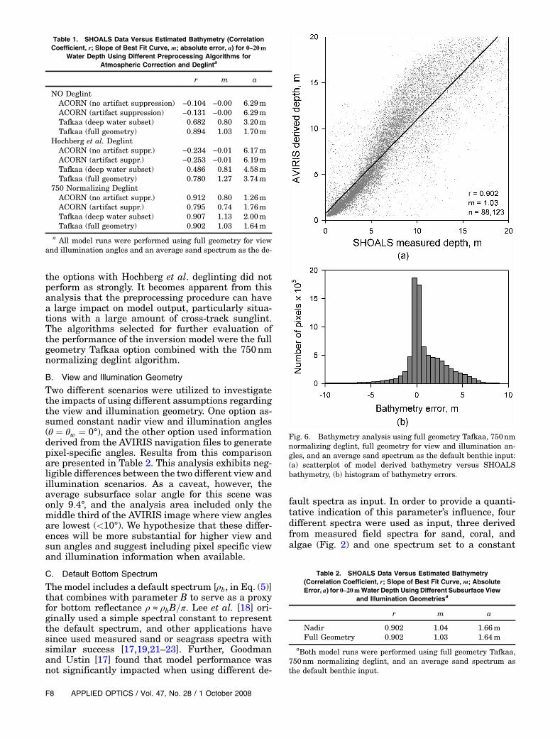
12 different preprocessing scenarios and performeda quantitative analysis of model estimated bathyme-try for each scenario using the SHOALS bathymetrydata as ground truth. Results from this analysis arepresented in Table 1, specifying the regression coef-ficient, r, the slope of linear least-squares fit, m, andthe average absolute difference, a, for each scenariofrom 0 to 20mwater depth. The best overall scenariowas the combination of full geometry Tafkaa with the750nm normalizing algorithm for deglinting. Thisscenario exhibited a strong, nearly one-to-one, corre-lation (r ¼ 0:9, m ¼ 1:03), with an average absolutedifference of 1:6m for depths from 1 to 20m (Fig. 6),which indicates a robust capacity for estimating

bathymetry. The strength of this relationship is alsoparticularly encouraging considering there are someacknowledged residual errors resulting from misre-gistration and spatial resampling. The best perfor-mance is achieved in depths from 0 to 7m, withoverestimation observed in depths greater than7m. Other applications of the inversion model haveshown strong bathymetric agreement for depths of15m or greater [19,23]. Hence, we attribute the over-estimation in this case to be a function of the wateroptical properties in Kaneohe Bay, where waterclarity is relatively limited compared with typicalreef environments.

Other promising results included the Tafkaa op-tion using the deep water subset and the ACORN op-tion with no artifact suppression, both combinedwith the 750nm normalizing algorithm, as well asthe full geometry Tafkaa option with no deglint(but all exhibiting either slightly lower regressioncoefficients or significantly lower slope than the bestoverall option). All other ACORN options and all of

Fig. 4. Remote sensing reflectance output following atmosphericcorrection and Hochberg et al. deglint algorithm: (a) 10-line cross-track average of deep water at 750nm, (b) 9-pixel average spectralprofile for submerged sand at 3m depth.

Fig. 5. Remote sensing reflectance output following atmosphericcorrection and 750 normalizing deglint algorithm: (a) 10-line cross-track average of deep water at 750nm, (b) 9-pixel average spectralprofile for submerged sand at 3m depth.


the options with Hochberg et al. deglinting did notperform as strongly. It becomes apparent from thisanalysis that the preprocessing procedure can havea large impact on model output, particularly situa-tions with a large amount of cross-track sunglint.The algorithms selected for further evaluation ofthe performance of the inversion model were the fullgeometry Tafkaa option combined with the 750nmnormalizing deglint algorithm.

B. View and Illumination Geometry

Two different scenarios were utilized to investigatethe impacts of using different assumptions regardingthe view and illumination geometry. One option as-sumed constant nadir view and illumination angles(θ ¼ θw ¼ 0°), and the other option used informationderived from the AVIRIS navigation files to generatepixel-specific angles. Results from this comparisonare presented in Table 2. This analysis exhibits neg-ligible differences between the two different view andillumination scenarios. As a caveat, however, theaverage subsurface solar angle for this scene wasonly 9:4°, and the analysis area included only themiddle third of the AVIRIS image where view anglesare lowest (<10°). We hypothesize that these differ-ences will be more substantial for higher view andsun angles and suggest including pixel specific viewand illumination information when available.

C. Default Bottom Spectrum

The model includes a default spectrum [ρb, in Eq. (5)]that combines with parameter B to serve as a proxyfor bottom reflectance ρ ≈ ρbB=π. Lee et al. [18] ori-ginally used a simple spectral constant to representthe default spectrum, and other applications havesince used measured sand or seagrass spectra withsimilar success [17,19,21–23]. Further, Goodmanand Ustin [17] found that model performance wasnot significantly impacted when using different de-

fault spectra as input. In order to provide a quanti-tative indication of this parameter’s influence, fourdifferent spectra were used as input, three derivedfrom measured field spectra for sand, coral, andalgae (Fig. 2) and one spectrum set to a constant

Table 1. SHOALS Data Versus Estimated Bathymetry (CorrelationCoefficient, r; Slope of Best Fit Curve, m; absolute error, a) for 0–20m

Water Depth Using Different Preprocessing Algorithms forAtmospheric Correction and Deglinta

r m a

NO DeglintACORN (no artifact suppression) −0:104 −0:00 6:29mACORN (artifact suppression) −0:131 −0:00 6:29mTafkaa (deep water subset) 0.682 0.80 3:20mTafkaa (full geometry) 0.894 1.03 1:70m

Hochberg et al. DeglintACORN (no artifact suppr.) −0:234 −0:01 6:17mACORN (artifact suppr.) −0:253 −0.01 6:19mTafkaa (deep water subset) 0.486 0.81 4:58mTafkaa (full geometry) 0.780 1.27 3:74m

750 Normalizing DeglintACORN (no artifact suppr.) 0.912 0.80 1:26mACORN (artifact suppr.) 0.795 0.74 1:76mTafkaa (deep water subset) 0.907 1.13 2:00mTafkaa (full geometry) 0.902 1.03 1:64m

a All model runs were performed using full geometry for viewand illumination angles and an average sand spectrum as the de-

Table 2. SHOALS Data Versus Estimated Bathymetry(Correlation Coefficient, r; Slope of Best Fit Curve, m; AbsoluteError, a) for 0–20mWater Depth Using Different Subsurface View

and Illumination Geometriesa

r m a

Nadir 0.902 1.04 1:66mFull Geometry 0.902 1.03 1:64m

aBoth model runs were performed using full geometry Tafkaa,750nm normalizing deglint, and an average sand spectrum asthe default benthic input.

Fig. 6. Bathymetry analysis using full geometry Tafkaa, 750nmnormalizing deglint, full geometry for view and illumination an-gles, and an average sand spectrum as the default benthic input:(a) scatterplot of model derived bathymetry versus SHOALSbathymetry, (b) histogram of bathymetry errors.


value of 1.0. Results were again analyzed by compar-ing estimated bathymetry with the measuredSHOALS data (Table 3). This comparison indicatesonly minor variations in the output, despite the dif-ferences in the input spectra. Even the flat spectrumproduced reasonable output. This favorable function-ality is attributed to the fact that optimization isa function of the entire spectrum from 400 to800nm, a region where the most significant influ-ence is attenuation in the water column, particularlyat longer wavelengths. Thus, the more minor differ-ences in spectral shape associated with the differentinput spectra are substantially less influential on theoptimization. This suggests that within reason themodel is not overly sensitive to the input spectrumand that it can be applied over diverse bottom fea-tures with minimal impact on performance.

D. Kernel Processing

A final bathymetry analysis was performed usingthree different kernel processing options: the default1 × 1 scenario, aswell as 3 × 3 and 5 × 5 kernel scenar-ios. Results are presented in Table 4, where it is evi-dent that the kernel processing option leads todecreasing accuracy for estimating bathymetry. Acomparison of other model output parameters con-firms that the processing scheme produces greater lo-cal uniformity in the water properties, as intended,but at the expense of introducing errors primarilyin the bathymetry. Such results are not entirely unex-pected, however, particularly in a model limited toonly five output parameters, where changes impartedon three of the parameters (P, G, BP) are manifest inchanges to the two other parameters (B,H). Further,the computational penalty for including thekernel op-tions increased processing time from 30min (desktopPC with 3:20GHz CPU and 1:0GB RAM) to 24 h forthe 3 × 3 kernel and over 6 days for the 5 × 5 kernel.Together, these results indicate that themodel shouldretain its original processing architecture of proces-sing each pixel independently.

E. Benthic Reflectance

Another measure of accuracy was evaluated by com-paring model-derived estimates of bottom reflec-tance at 550nm with measured data at 12 sandareas in Kaneohe Bay. The 12 areas were locatedat depths varying from 0.5 to 15:5m and spatially

distributed throughout the bay. Average, minimum,and maximum reflectance values at 550nm were ex-tracted from the merged 2001 and 2002 field data,which were assumed to be representative of reflec-tance at these same areas in 2000. Additionally, be-cause each of the selected sand areas was reasonablyhomogeneous, it was also assumed that the averagecharacteristics extracted from the 40–60 point sam-ples at each field location were equivalent to averagemodel estimates at the scale of image pixels. Valuesfor model estimated reflectance at 550nm (B) wereextracted from the image areas corresponding toeach of the field sampling locations. Figure 7 illus-trates results of the reflectance estimate differencesat 550nm from all 12 sand areas. Reflectance esti-mates for each area are within the range of measuredfield data for the majority of the sand areas, and therelative levels of reflectance also generally parallelthe trends of lighter and darker sand areas (but withan average positive offset of 9.6%). This offset is par-tially attributed to scaling errors associated withcomparing field measurements with image databut is also suggestive of the need to incorporate afixed parameter resembling Q for optically shallowwaters [41] (Q ¼ Eu=Lu, the ratio of upwelling irradi-ance to upwelling radiance at nadir) in the equationfor bottom reflectance (e.g., ρ ≈ ρbB=Q, with Q < π),rather than the current formulation using π to con-vert between the radiance and irradiance fields. Inthis example, Q ¼ 2:6 would significantly improvethe comparison of estimated reflectance with mea-sured sand reflectance for the 12 sand areas (redu-cing the average difference to 3%), which is in linewith Q values for shallow sand areas measured byVoss et al.[41]. This avenue of research warrantsfurther investigation. Nonetheless, because of thegeneral consistency in the reflectance offset, whichdid not appear to adversely affect the bathymetry es-timates, results from the current model formulationwere deemed reasonable.

5. Conclusions

Numerous different scenarios were utilized in eval-uating output from the semi-analytical model usingAVIRIS data from Kaneohe Bay. Model accuracy wasprimarily assessed using SHOALS bathymetry databut also using measured field reflectance spectra. Re-sults indicated that the most significant influence on

Table 3. SHOALS Data Versus Estimated Bathymetry(Correlation Coefficient, r; Slope of Best Fit Curve, m;

Absolute Error, a) for 0–20m Water Depth Using DifferentDefault Bottom Spectra as Model Inputa

r m a

Sand 0.902 1.03 1:64mCoral 0.902 0.99 1:48mAlgae 0.902 1.00 1:50mFlat 0.901 0.96 1:40m

aAll model runs were performed using full geometry Tafkaa,750nm normalizing deglint, and full geometry for view and illumi-nation angles.

Table 4. SHOALS Data Versus Estimated Bathymetry(Correlation Coefficient, r; Slope of Best Fit Curve, m;

Absolute Error, a) for 0–20m Water Depth Using DifferentSpatial Kernels for Averaging Water Propertiesa

r m a

1 × 1 0.902 1.03 1:64m3 × 3 0.801 0.85 1:89m5 × 5 0.801 0.81 1:88m

aAll model runs performed using full geometry Tafkaa, 750nmnormalizing deglint, full geometry for view and illumination an-gles, and an average sand spectrum as the default benthic input.


model output was the selection of preprocessingschemes. The best preprocessing option of those con-sidered in this study was the full geometry Tafkaaoption for atmospheric correction combined with astraightforward 750nm normalizing algorithm fordeglinting. Results also indicated that incorporatingexplicit view and illumination geometries within theinversion model has insignificant impact at smallerangles, that the model is not significantly affected bychanges in the default bottom spectrum and that akernel processing scheme for averaging water prop-erties produces decreased accuracy in the bathyme-try estimates. By testing and validating the modelusing AVIRIS imagery from Kaneohe Bay, Hawaii,results from this analysis have demonstrated modeltransferability and also provided further evidence ofits reliability and robust performance capabilities.Furthermore, despite previous limitations on theavailability of hyperspectral instruments, whichwere often limited to research investigations (e.g.,AVIRIS, PHILLS), the accessibility and number ofcommercial airborne instruments continues to in-crease (e.g., HyMap, CASI, AISA), and even space-borne data from HYPERION is now available.Therefore, application of the semi-analytical modelultimately extends an important analysis tool to a di-versity of other shallow aquatic ecosystems.

This work was supported by NASA Headquartersunder Earth System Science Fellowship GrantNGT5-ESS/01-0000-0208. It was also supported byGordon-CenSSIS, the Bernard M. Gordon Centerfor Subsurface Sensing and Imaging Systems, under

the Engineering Research Centers Program ofthe National Science Foundation (Award NumberEEC-9986821). Additional assistance was providedby the Center for Spatial Technologies and RemoteSensing, the University of California Pacific RimResearch Program, the California Space InstituteGraduate Student Fellowship Program, the CanonNational Park Science Scholars Program, andNASA’s Jet Propulsion Laboratory. Appreciation isalso extended to M. Montes and C. Davis at theU.S. Naval Research Laboratory for the Tafkaamodel, the U.S. Army Corps of Engineers for theSHOALS bathymetry data, D. Riano for processingof the SHOALS data, the Hawaii Institute of MarineBiology for their support, and P. Sjordal for his untir-ing assistance in the field.

References1. V. E. Brando and A. G. Dekker, “Satellite hyperspectral

remote sensing for estimating estuarine and coastal waterquality,” IEEE Transactions on Geoscience and Remote Sen-sing 41, 1378–1387 (2003).

2. K. L. Carder, P. Reinersman, R. F. Chen, F. Muller-Karger,C. O. Davis, and M. Hamilton, “AVIRIS calibration and appli-cation in coastal oceanic environments,” Remote Sens. Envir-on. 44, 205–216 (1993).

3. L. L. Richardson, “Remote sensing of algal bloom dynamics,”BioScience 46, 492–501 (1996).

4. S. Thiemann and H. Kaufmann, “Lake water quality monitor-ing using hyperspectral airborne data—a semiempirical mul-tisensor and multitemporal approach for the MecklenburgLake District, Germany,” Remote Sens. Environ. 81, 228–237(2002).

5. M. K. Hamilton, C. O. Davis, W. J. Rhea, S. H. Pilorz, andK. L. Carder, “Estimating chlorophyll content and bathymetryof Lake Tahoe using AVIRIS data,” Remote Sens. Environ. 44,217–230 (1993).

6. E. J. Hochberg and M. J. Atkinson, “Capabilities of remotesensors to classify coral, algae, and sand as pure and mixedspectra,” Remote Sens. Environ. 85, 174–189 (2003).

7. E. J. Hochberg and M. J. Atkinson, “Spectral discrimination ofcoral reef benthic communities,” Coral reefs : Journal of theInternational Society for Reef Studies 19, 164–171(2000).

8. P. J. Mumby, W. Skirving, A. E. Strong, J. T. Hardy,E. F. LeDrew, E. J. Hochberg, R. P. Stumpf, and L. D. David,“Remote sensing of coral reefs and their physical environ-ment,” Mar. Pollution Bull. 48, 219–228 (2004).

9. D. Lubin, W. Li, P. Dustan, C. H. Mazel, and K. Stamnes,“Spectral signatures of coral reefs: features from space,” Re-mote Sens. Environ. 75, 127–137 (2001).

10. S. Bagheri, M. Stein, and R. Dios, “Utility of hyperspectraldata for bathymetric mapping in a turbid estuary,” Int. J. Re-mote Sens. 19, 1179–1188 (1998).

11. J. C. Sandidge and R. J. Holyer, “Coastal bathymetry from hy-perspectral observations of water radiance,” Remote Sens. En-viron. 65, 341–352 (1998).

12. D. Durand, J. Bijaoui, and F. Cauneau, “Optical remote sen-sing of shallow-water environmental parameters: a feasibilitystudy,” Remote Sens. Environ. 73, 152–161 (2000).

13. E. M. Louchard, R. P. Reid, F. C. Stephens, C. O. Davis,R. A. Leathers, and T. V. Downes, “Optical remote sensingof benthic habitats and bathymetry in coastal environmentsat Lee Stocking Island, Bahamas: a comparative spectralclassification approach,” Limnol. Oceanogr. 48, 511–521(2003).

Fig. 7. Comparison of model derived reflectance at 550nm versusmeasured data at 12 sand target areas; model derivation per-formed using full geometry Tafkaa, 750nm normalizing deglint,full geometry for view and illumination angles, and an averagesand spectrum as the default benthic input.


14. H. M. Dierssen, R. C. Zimmerman, R. A. Leathers,T. V. Downes, and C. O. Davis, “Ocean color remote sensingof seagrass and bathymetry in the Bahamas Banks byhigh-resolution airborne imagery,” Limnol. Oceanogr. 48,444–455 (2003).

15. J. D. Hedley and P. J. Mumby, “A remote sensing method forresolving depth and subpixel composition of aquatic benthos,”Limnol. Oceanogr. 48, 480–488 (2003).

16. M. P. Lesser and C. D. Mobley, “Bathymetry, water opticalproperties, and benthic classification of coral reefs using hy-perspectral imagery,”Coral reefs : Journal of the InternationalSociety for Reef Studies 26, 819–829 (2007).

17. J. Goodman and S. L. Ustin, “Classification of benthic compo-sition in a coral reef environment using spectral unmixing,” J.Appl. Remote Sens. 1, 011501 (2007).

18. Z. Lee, K. Carder, C. D. Mobley, R. Steward, and J. Patch,“Hyperspectral remote sensing for shallow waters. 1. a semi-analytical model,” Appl. Opt. 37, 6329–6338 (1998).

19. Z. Lee, K. Carder, C. D. Mobley, R. Steward, and J. Patch,“Hyperspectral remote sensing for shallow waters: 2. derivingbottom depths and water properties by optimization,” Appl.Opt. 38, 3831–3843 (1999).

20. C. D. Mobley, L. K. Sundman, C. O. Davis, J. H. Bowles,T. V. Downes, R. A. Leathers, M. J. Montes, W. P. Bisset,D. D. R. Kohler, R. P. Reid, E. M. Louchard, and A. Gleason,“Interpretation of hyperspectral remote-sensing imagery byspectrum matching and look-up tables,” Appl. Opt. 44,3576–3592 (2005).

21. Z. Lee, K. L. Carder, R. F. Chen, and T. G. Peacock, “Propertiesof the water column and bottom derived from Airborne VisibleInfrared Imaging Spectrometer (AVIRIS) data,” J. Geophys.Res. 106, 11639–11651 (2001).

22. Z. Lee and K. L. Carder, “Effect of spectral band numbers onthe retrieval of water column and bottom properties fromocean color data,” Appl. Opt. 41, 2191–2201 (2002).

23. Z. Lee, B. Casey, R. Arnone, A. Weidemann, R. Parsons,M. J. Montes, B.-C. Gao, W. Goode, C. O. Davis, and J. Dye,“Water and bottom properties of a coastal environment de-rived from Hyperion data measured from the EO-1 spacecraftplatform,” J. Appl. Remote Sens. 1, 011502 (2007).

24. J. A. Goodman, M. Velez-Reyes, S. Hunt, and R. Armstrong,“Development of a field test environment for the validationof coastal remote sensing algorithms: Enrique Reef, PuertoRico,” in Remote Sensing of the Ocean, Sea Ice, and LargeWater Regions, C. R. Bostater, X. Neyt, S. P. Mertikas, andM. Velez-Reyes, eds. (SPIE, 2006), p. 8.

25. E. J. Hochberg, S. Andrefouet, and M. R. Tyler, “Sea surfacecorrection of high spatial resolution Ikonos images to improvebottom mapping in near-shore environments,” IEEE Trans.Geosci. Remote 41, 1724–1729 (2003).

26. G. Vane, R. O. Green, T. G. Chrien, H. T. Enmark,E. G. Hansen, andW. M. Porter, “The airborne visible/infrared

imaging spectrometer (AVIRIS),” Remote Sens. Environ. 44,127–143 (1993).

27. R. O. Green, M. L. Eastwood, C. M. Sarture, T. G. Chrien,M. Aronsson, B. J. Chippendale, J. A. Faust, B. E. Pavri,C. J. Chovit, M. Solis, M. R. Olah, and O. Williams, “Imagingspectroscopy and the Airborne Visible/Infrared Imaging Spec-trometer (AVIRIS),” Remote Sens. Environ. 65, 227–248(1998).

28. J. L. Irish and W. J. Lillycrop, “Scanning laser mapping of thecoastal zone: the SHOALS system,” ISPRS J. Photogramm.Remote Sens. 54, 123–129 (1999).

29. J. L. Irish, J. K. McClung, and W. J. Lillycrop, “Airborne lidarbathymetry: the SHOALS system,” PIANC Bull. 103-2000,43–53 (2000).

30. J. A. Goodman and S. L. Ustin, “Underwater spectroscopy:methods and applications in a coral reef environment,” pre-sented at the 7th International Conference on Remote Sen-sing for Marine and Coastal Environments, Miami, Florida,USA, 20–22 May 2002.

31. J. A. Goodman and S. L. Ustin, “Acquisition of underwater re-flectance measurements as ground truth,” presented at the11th JPL Airborne Earth Science Workshop, Jet PropulsionLaboratory, California, USA, 4–8 March 2002.

32. M. J. Montes, Naval Research Laboratory, Code 7232,Washington, D.C., 20375, (personal communication, 2005).

33. T. Heege and J. Fischer, “Sun glitter correction in remote sen-sing imaging spectrometry,” in SPIE Ocean Optics XV (SPIE,2000), p. 11.

34. L. Analytical Imaging and Geophysics, “ACORN 4.0 User’sGuide,” (ImSpec, LLC, Boulder, CO, 2002).

35. B.-C. Gao, M. J. Montes, Z. Ahmad, and C. O. Davis, “Atmo-spheric correction algorithm for hyperspectral remote sensingof ocean color from space,” Appl. Opt. 39, 887–896 (2000).

36. M. J. Montes, B.-C. Gao, and C. O. Davis, “A new algorithm foratmospheric correction of hyperspectral remote sensing data,”Proc. SPIE 4383, 23–30 (2001).

37. M. Montes, B.-C. Gao, and C. O. Davis, “Tafkaa atmosphericcorrection of hyperspectral data,” Proc. SPIE 5159, 188–197(2003).

38. B.-C.GaoandA.F.H.Goetz, “Columnatmosphericwater vaporand vegetation liquid water retrievals from airborne imagingspectrometer data,” J. Geophys. Res. 95, 3549–3564 (1990).

39. B.-C. Gao, K. B. Heidebrecht, and A. F. H. Goetz, AtmosphericRemoval Program (ATREM) User’s Guide (University of Col-orado at Boulder, 1992).

40. J. D. Hedley, A. R. Harborne, and P. J. Mumby, “Simple androbust removal of sun glint for mapping shallow-waterbenthos,” Int. J. Remote Sens. 26, 2107–2112 (2005).

41. K. J. Voss, C. D. Mobley, L. K. Sundman, J. E. Ivey, andC. H. Mazel, “The spectral upwelling radiance distributionin optically shallow waters,” Limnol. Oceanogr. 48, 364–373 (2003).


influence of atmospheric and sea-surface corrections on retrieval of bottom depth and reflectance...

Documents