influence of environment induced correlated fluctuations

Influence of environment induced correlated fluctuations in electroniccoupling on coherent excitation energy transfer dynamics in modelphotosynthetic systemsPengfei Huo and David F. Coker Citation: J. Chem. Phys. 136, 115102 (2012); doi: 10.1063/1.3693019 View online: http://dx.doi.org/10.1063/1.3693019 View Table of Contents: http://jcp.aip.org/resource/1/JCPSA6/v136/i11 Published by the American Institute of Physics. Additional information on J. Chem. Phys.Journal Homepage: http://jcp.aip.org/ Journal Information: http://jcp.aip.org/about/about_the_journal Top downloads: http://jcp.aip.org/features/most_downloaded Information for Authors: http://jcp.aip.org/authors

Downloaded 27 Apr 2012 to 131.215.220.186. Redistribution subject to AIP license or copyright; see http://jcp.aip.org/about/rights_and_permissions

http://jcp.aip.org/?ver=pdfcov

http://aipadvances.aip.org/resource/1/aaidbi/v2/i1?&section=special-topic-physics-of-cancer&page=1

http://jcp.aip.org/search?sortby=newestdate&q=&searchzone=2&searchtype=searchin&faceted=faceted&key=AIP_ALL&possible1=Pengfei Huo&possible1zone=author&alias=&displayid=AIP&ver=pdfcov

http://jcp.aip.org/search?sortby=newestdate&q=&searchzone=2&searchtype=searchin&faceted=faceted&key=AIP_ALL&possible1=David F. Coker&possible1zone=author&alias=&displayid=AIP&ver=pdfcov


http://link.aip.org/link/doi/10.1063/1.3693019?ver=pdfcov

http://jcp.aip.org/resource/1/JCPSA6/v136/i11?ver=pdfcov

http://www.aip.org/?ver=pdfcov


http://jcp.aip.org/about/about_the_journal?ver=pdfcov

http://jcp.aip.org/features/most_downloaded?ver=pdfcov

http://jcp.aip.org/authors?ver=pdfcov

THE JOURNAL OF CHEMICAL PHYSICS 136, 115102 (2012)

Influence of environment induced correlated fluctuations in electroniccoupling on coherent excitation energy transfer dynamics in modelphotosynthetic systems

Pengfei Huo1,2 and David F. Coker1,3,a)

1Department of Chemistry, Boston University, 590 Commonwealth Avenue, Boston, Massachusetts 02215, USA2Division of Chemistry and Chemical Engineering, California Institute of Technology, Pasadena,California 91125, USA3Department of Physics, and Complex Adaptive Systems Laboratory, University College Dublin,Dublin 4, Ireland

(Received 30 December 2011; accepted 22 February 2012; published online 15 March 2012)

Two-dimensional photon-echo experiments indicate that excitation energy transfer between chro-mophores near the reaction center of the photosynthetic purple bacterium Rhodobacter sphaeroidesoccurs coherently with decoherence times of hundreds of femtoseconds, comparable to the energytransfer time scale in these systems. The original explanation of this observation suggested that cor-related fluctuations in chromophore excitation energies, driven by large scale protein motions couldresult in long lived coherent energy transfer dynamics. However, no significant site energy corre-lation has been found in recent molecular dynamics simulations of several model light harvestingsystems. Instead, there is evidence of correlated fluctuations in site energy-electronic coupling andelectronic coupling-electronic coupling. The roles of these different types of correlations in excitationenergy transfer dynamics are not yet thoroughly understood, though the effects of site energy correla-tions have been well studied. In this paper, we introduce several general models that can realisticallydescribe the effects of various types of correlated fluctuations in chromophore properties and system-atically study the behavior of these models using general methods for treating dissipative quantumdynamics in complex multi-chromophore systems. The effects of correlation between site energy andinter-site electronic couplings are explored in a two state model of excitation energy transfer betweenthe accessory bacteriochlorophyll and bacteriopheophytin in a reaction center system and we findthat these types of correlated fluctuations can enhance or suppress coherence and transfer rate simul-taneously. In contrast, models for correlated fluctuations in chromophore excitation energies showenhanced coherent dynamics but necessarily show decrease in excitation energy transfer rate accom-panying such coherence enhancement. Finally, for a three state model of the Fenna-Matthews-Olsenlight harvesting complex, we explore the influence of including correlations in inter-chromophorecouplings between different chromophore dimers that share a common chromophore. We find thatthe relative sign of the different correlations can have profound influence on decoherence time andenergy transfer rate and can provide sensitive control of relaxation in these complex quantum dy-namical open systems. © 2012 American Institute of Physics. [http://dx.doi.org/10.1063/1.3693019]

I. INTRODUCTION

The results of two-dimensional nonlinear spectroscopyexperimental studies show the signature of long livedquantum coherent dynamics in a wide variety of nano-structured systems involving chromophores embedded inpolymeric scaffoldings such as photosynthetic light har-vesting systems1–5 and conducting polymers.6 One of thefirst experimental papers reporting this phenomenon in thechromophores around a chemically modified reaction cen-ter model suggested that the mechanism for this long livedcoherence1 involved collective motion in the nano-structuredenvironment that led to correlated fluctuations in chro-mophore excitation energies. This mechanism for coherentelectronic excitation energy transfer has also been suggested

a)Electronic mail: [email protected].

in studies on DNA,9, 10 and a similar mechanism has beenshown to be operative for coherent vibrational excitation en-ergy transfer in various model systems.7, 8 Scholes and co-workers2 have suggested that in certain light harvesting com-plexes such as PC645 or PE545 from cryptophyte algae wherethe chromophores are covalently bonded to the protein back-bone, this type of correlation might be larger compared to reg-ular harvesting complexes in which the chromophores simplyintercalate into the protein structure.

Recent molecular dynamics (MD) simulation studies onthe Fenna-Mathews-Olsen (FMO) excitation energy transfernetwork,11, 12 the light harvesting complex 2 (LHII) photo-synthetic light harvesting complex13 and the reaction cen-ter complex,14 however, show no significant correlation insite energy fluctuations after averaging, and similar findingshave been reported from calculations for the PE54515 lightharvesting system. However, Kleinekathöfer and co-workers,

0021-9606/2012/136(11)/115102/17/$30.00 © 2012 American Institute of Physics136, 115102-1


http://dx.doi.org/10.1063/1.3693019

http://dx.doi.org/10.1063/1.3693019

http://dx.doi.org/10.1063/1.3693019

http://dx.doi.org/10.1063/1.3693019

mailto: [email protected]

115102-2 P. Huo and D. F. Coker J. Chem. Phys. 136, 115102 (2012)

for example, have found that in FMO,11 there is evidence ofcorrelations in fluctuations of site energy and inter site elec-tronic couplings and electronic coupling-electronic couplingcorrelations that are more significant compared to the appar-ently uncorrelated site energy fluctuations. There have beenquestions raised in recent work about the magnitudes of theparameters used, and the assumptions underlying some ofthese model calculations.12, 14 There have also been sugges-tions that the mechanism by which correlated fluctuations insite-energies average out is dynamically more subtle, occur-ring through the washing out of correlated and anti-correlatedsite energy fluctuations at different frequencies.12 The goalof this paper, however, is to study the qualitative character-istics of a different class of models that have received littleattention. This paper will thus systematically explore the in-fluence of correlations involving electronic couplings on thequantum dynamics in a model for excitation energy transferprocesses between the accessory chlorophyll (Bchl or B) andpheophytin (Bphy or H) in the bacterial reaction center ofRhodobacter sphaeroides,1 the system that was the subject ofthe early experimental studies where coherent excitation en-ergy transfer was observed by Fleming and co-workers men-tioned above. We also present results exploring the effects ofsuch correlations on the population transfer and coherence ina simplified three state model of the FMO light harvestingcomplex.

There is a rich literature exploring various models forcorrelated environmental fluctuations.16–22 Detailed system-bath interaction models have also been developed includ-ing a cross-coupling model23 and the common bath couplingmodel.8, 9, 24–26 All of these studies so far incorporate the ef-fects of correlation between fluctuations in the excitation en-ergies of different sites. As suggested above, other possi-ble correlations between site energy and inter-site couplingfluctuations may be considered. The possible origin of suchcorrelations could be bath modes that influence the relativedistances, and angles between two transition dipoles of dif-ferent chromophores.27 Some MD simulations suggest thatcorrelated fluctuations in electronic coupling between chro-mophore dimer pairs that share a common chromophore,11 forexample, correlation between 4–5 coupling and 5–7 couplingin the FMO complex (i.e., inter-site coupling-inter-site cou-pling correlations) may be significant and one of the primarygoals of this paper is to explore the effects of such correlationon the quantum dynamics of model chromophore networks.The simplified systems we explore in this paper thus includeboth a two state model where we can single out the effects ofsite energy-inter-site coupling correlations, and a three stateexample that is a minimal model in which inter-site coupling-inter-site coupling correlation can be explored.

Chen and Silbey28 and others29 recently used an ex-tended Haken-Strobl-Reineker (HSR) model that not onlyincludes the site energy correlations but also the siteenergy-inter-site electronic coupling correlations to study theinfluence of different types of correlation for a simple twostate model. Their work28 clearly shows that if we also in-clude the effect of the correlation between inter-site electroniccoupling fluctuation27 and site energy fluctuation, the coher-ent nature of the excitation energy transfer dynamics can be

strongly enhanced or suppressed depending on the sign ofthese correlations. Further, Jang27 also showed that if an in-dependent bath is coupled to the off-diagonal element in atwo state model, this will always enhance the excitation en-ergy transfer rate (assuming that the bath only influences thedistance between the two dipoles). Coalson and co-workers30

recently used the polaron transformation to study the non-Condon effect on a model electron transfer process by in-cluding the possibility that the environmental bath can alsocouple to the off-diagonal element in the spin-boson prob-lem. This study addresses essentially the same type of ques-tion as the influence of the bath on the off-diagonal couplingin the excitation energy transfer model described by Chen andSilbey,28 however, Coalson and co-workers neglected the pos-sibility that the relative sign of the off-diagonal coupling canprofoundly change the dynamics.

In this work, we evolve the quantum dynamics of the fullmulti-chromophore light harvesting system coupled, via var-ious bi-linear interaction models of increasing complexity, todifferent sets of harmonic bath modes. The approach we em-ploy to perform these large scale dissipative open quantumsystem simulations is our recently developed approximatesemi-classical approach that linearizes the density matrix evo-lution in the difference between forward and backward pathsof the environmental degrees of freedom (DOF)31, 32 whilekeeping interference effects between forward and backwardpaths of the system DOF.33 This new approach is known as thepartial linearized density matrix (PLDM) dynamics scheme34

and it is a highly efficient variant of our earlier iterative lin-earized density matrix (ILDM) propagation method.35–37 ThePLDM propagation approach is outlined in Sec. S.1 of thesupplemental materials for this article.39 In this paper thisapproximate quantum dynamics scheme is employed to studythe effects of correlations between fluctuations in site en-ergies and inter-site electronic couplings on coherent ex-citation energy transfer dynamics in a two state reactioncenter model and a three state excitation energy transfer net-work. These quantum propagation methods do not suffer fromthe limitations of the approximations inherent in many tradi-tional approaches such as Foerster Resonant Energy Transfer(FRET) theory38 and the Redfield or Lindblad equations,40 orthe HSR model for dynamics that assumes infinite temper-ature and cannot accurately capture finite temperature equi-libration at longer times. The new partial linearized versionand ILDM propagation approaches have been used36 to con-duct benchmark comparisons with results from various othermethods41, 42 and have been shown to be very reliable fora wide variety of applications. Particularly important fea-tures of these new methods are their general applicability toarbitrary non-Markovian system-bath spectral densities andbeyond bi-linear coupling models. Also these methods arenon-perturbative, enhancing their applicability to a diverserange of problems. The trajectory implementation, particu-larly in the case of the PLDM propagation approach, makesthis method extremely numerically efficient.

In this paper, we employ these approaches to studygeneralized non-Markovian models. Nevertheless, the resultsof our studies suggest that the findings from the approxi-mate theoretical calculations of Chen and Silbey are gen-



eral and robust. In particular we find that the correlationbetween site energy and off-diagonal inter-site coupling, andinter-site-inter-site coupling correlations can either enhanceor suppress the survival of coherence and the excitation en-ergy transfer rate depending on the type of correlation (posi-tive or negative correlation) just as Chen and Silbey find withtheir approximate calculations on simplified models. In an-other calculation on a three state model for FMO we explorevarious possible correlations, and find that the excitation en-ergy transfer rate is strongly influenced by the relative sign ofthe correlations, and the same is true for the magnitude of thelong lived coherent oscillations in off-diagonal density matrixelements. Further, with these types of correlated fluctuationsthe trends in the excitation energy transfer rate are not signifi-cantly effected relative to the magnitude and decay time of thecoherence, which means that for bigger coherence comparedto the independent bath model, the exciton transfer rate couldbe faster or slower, and for smaller coherence, the transfer ratecould also be bigger or smaller, depending on the relative signof the different types of correlations. These studies thus sug-gest that if these types of correlated fluctuations are operative,the observed coherent dynamics in the experiments is unlikelyto play a significant role in the mechanism for excitation en-ergy transfer in these systems, as its presence does not pointespecially to enhancement of energy transport processes.

II. MODEL SYSTEMS

The experimental results1 that motivate our first set ofmodel studies were performed on chromophores embedded inthe transmembrane protein scaffolding near the reaction cen-ter of Rhodobacter sphaeroides. In these experiments the pri-mary electron donor (the special pair) is chemically oxidized,shutting down the electron transfer43 so that only excitedstate energy transfer between the accessory bacteriochloro-phyll (Bchl or B) and bacteriopheophytin (BPhy, or H) is pos-sible. The 2D photon echo experiments by Lee et al.1 showeda long lived beating signal associated with |H〉〈B| coherentdynamics. These authors found that they could fit this spec-tral dynamics reasonably by assuming the fluctuations in theB and H site energies were strongly correlated, and suggestedthat in-phase energy fluctuations could be responsible for pre-serving coherence.1 It was found that strong electronic cou-pling, which could also lead to longer lived coherence, wouldnot, however, give a reasonable fit to experimental data.1 Weexplore their correlated site energy fluctuation model in de-tailed calculations presented in Appendix. Below, however,we present an alternative model Hamiltonian that includescorrelated fluctuations between chromophore excitation en-ergies and electronic couplings that we show can equally wellreproduce the underlying density matrix dynamics probed inthe experimental signals.

A. A model Hamiltonian for correlatedfluctuations in chromophore excitation energiesand inter-chromophore electronic couplings

The model system Hamiltonian that has been determinedby fitting the experimental data for coherent excitation en-

ergy transfer dynamics between the H and B chromophoresin the chemically modified reaction center model is presentedin complete detail below, and in Appendix.1 In addition tovariations on the three components outlined here, this experi-mentally determined Hamiltonian includes a Brownian oscil-lator mode that modulates the excitation energy of the accep-tor state |B〉. This modulation is important to reproduce thedifferent oscillatory features observed in the experimental sig-nals, in particular the low frequency modulation as we showin Appendix. For the purpose of exploring the factors that in-fluence the electronic quantum coherent dynamics, however,the Brownian mode is a complication that we omit in thesestudies of the influence of correlated fluctuations in the siteand coupling terms.

Here we focus only on the electronic subsystem, bath,and system-bath coupling terms and assume the total Hamil-tonian has the following form:

H = Hs + Hs−b + Hb, (1)

where the electronic part of the Hamiltonian is

Hs =(

εH �(0)HB

�(0)BH εB

)=(

680 210

210 0

), (2)

and all the parameter values are given in cm−1. In this section,we explore the situation in which the inter-site off-diagonalcoupling bath and the bath that causes fluctuations in siteenergies are correlated. For simplicity, we assume that allthe modes that couple to |H〉〈H| and |B〉〈B| also couple to|H〉〈B| and |B〉〈H|. However, the modes coupled to |H〉〈H|and the modes coupled to |B〉〈B| are independent. With theabove assumption, the bi-linear system-bath and harmonicbath Hamiltonians can be written as

Hs−b = UHH + UBB + [UHB + UBH ] (3)

=n(H )∑l=1

c(H )l q

(H )l |H 〉〈H | +

n(B)∑l=1

c(B)l q

(B)l |B〉〈B|

+{

k(H )n(H )∑l=1

c(H )l q

(H )l + k(B)

n(B)∑l=1

c(B)l q

(B)l

}

× [|H 〉〈B| + |B〉〈H |]and

Hb = HHb + H B

b =n(H )∑l=1

1

2

[p

(H )2

l + ω(H )2

l q(H )2

l

](4)

+n(B)∑l=1

1

2

[p

(B)2

l + ω(B)2

l q(B)2

l

],

respectively, and [HHb , H B

b ] = 0, due to the independence ofdifferent chromophore baths. With this model, k(B) and k(H)

simply modulate the strength with which the independent{q(B)

l } and {q(H )l } bath degrees of freedom influence the inter-

site off-diagonal electronic coupling. The assumed form ofthe bath coordinate dependent electronic coupling with this



model is thus,

�HB

({q

(H )l

},{q

(B)l

}) = �(0)HB +

{k(H )

n(H )∑l=1

c(H )l q

(H )l

+ k(B)n(B)∑l=1

c(B)l q

(B)l

}. (5)

The physical idea underlying this form is that �(0)HB arises

from the interaction between transition dipoles in the refer-ence geometry, so within this dipole approximation,

�(0)HB = [μH · μB − 3(μH · nHB)(μB · nHB)]/εR3

HB,

(6)where, μH, say, is the transition dipole moment vector of theH chromophore, and nHB = RHB/RHB, with RHB = |RHB|, theinter-chromophore distance in the reference geometry. Thesecond term in Eq. (5) represents, for example, the processby which modes in the bath of chromophore B, i.e., {q(B)

l },modify the transition dipole moment, μB, and effect the elec-tronic coupling with chromophore H as the bath causes fluc-tuations about the reference geometry. This bath coordinatedependent inter chromophore coupling term thus provides amechanism where by the independent baths of different chro-mophores can simultaneously influence a given term in theelectronic Hamiltonian and thus lead to fluctuations in elec-tronic excitation energies that are correlated to motions of thedifferent sets of otherwise independent bath modes.

Making the usual assumptions underlying linear re-sponse theory, the properties of the system-bath interac-tion of interest here are determined by the relevant ther-mal averaged equilibrium correlation functions. For ourconsiderations the site energy and inter-site off-diagonal cou-pling fluctuation correlation function terms, e.g., CHH,HB(t)= 〈〈H |Hs−b|H 〉(t)〈H |Hs−b|B〉(0)〉, have the forms,

CHH,HB(t) = 〈UHH (t)UHB(0)〉 (7)

= kBT k(H )n(H )∑l=1

c(H )2l

ω(H )2l

cos(ω

(H )l t)

= kBT

πk(H )∫ ∞

0dω

j (H )(ω)

ωcos(ωt),

CBB,HB(t) = 〈UBB(t)UHB(0)〉 (8)

= kBT k(B)n(B)∑l=1

c(B)2l

ω(B)2l

cos(ω

(B)l t)

= kBT

πk(B)∫ ∞

0dω

j (B)(ω)

ωcos(ωt),

where the angle brackets indicate thermal equilibrium ensem-ble averages, and here there are no cross terms in CHH, HB(t)or CBB, HB(t) related to 〈qH (t)qB(0)〉 due to the indepen-dent nature of HH

b and H Bb . These expressions define the

relevant spectral densities, j(B)(ω) and j(H)(ω) that, in this

model, determine both the dissipation of excitation energyfrom the sites to their environment and how the bath modeof frequency ω correlates fluctuations in the site energies andinter-chromophore electronic couplings. These spectral densi-ties, for example, have the following form in terms of modelsystem-bath interaction parameters:

j (H )(ω) = π

2

n(H )∑l=1

c(H )2l

ω(H )l

δ(ω − ω

(H )l

). (9)

For simplicity, with all the models considered here weassume that the spectral density that determines how the bathcorrelates different fluctuations has the same frequency de-pendence as the environmental interactions that dissipate siteenergy and the ks simply scale the magnitude of these inter-actions to give their contribution to a given correlated fluctu-ation. In the absence of further information about these typesof frequency dependent correlations this type of model seemsa reasonable first step. Calculations are currently underwayto explore the appropriateness of this model for realisticapplications.

The HSR two state system-bath model that providesthe basis of the simplified theoretical analysis of the in-fluence of correlations in site energy-inter-site coupling isbased on more restrictive approximations. The HSR modelassumes infinite temperature (T → ∞) and that the correla-tion functions governing the system-bath interactions are in-finitely rapidly decaying and makes the Markovian assump-tion, i.e., Ci,j,i ′,j ′ (t − t ′) = Ci,j,i ′,j ′ (0)δ(t − t ′). Despite thesesignificant limitations, the HSR model offers some interest-ing predictions about how correlated fluctuations influencethe coherent energy transfer in such dissipative quantum sys-tems. According to the solution of the HSR model presentedrecently by Chen and Silbey,28 the oscillation amplitude of thepopulation and off-diagonal coherence terms in the densitymatrix and other dynamical properties depend predominatelyon the sign of the difference in the amplitudes of these siteenergy-inter-site electronic coupling fluctuation correlationfunctions, i.e., with in the Markovian approximation the zerotime amplitude difference given by the quantity [CHH, HB(0)− CBB, HB(0)] plays a central role determining many dynam-ical properties. Thus, for example, Chen and Silbey find thatthe excitation energy transfer rate involves terms such as∼cos θsin θ [CHH, HB(0) − CBB, HB(0)] (Ref. 28) for their ap-proximate analytic model. Here the mixing angle, θ , governsthe transformation between the site and exciton (delocalizedeigenstates of Hs) representations and tan θ = −2�HB/(εH −εB) with (εH − εB) > 0. For example, their results suggestthat when tan θ < 0 (i.e., when �HB > 0), negative valuesof [CHH, HB(0) − CBB, HB(0)] will increase the amplitude ofthe oscillatory behavior of population and enhance the energytransfer rate, while positive values of this correlation func-tion difference will decrease these effects.28 To summarizeif the sign of the correlation function difference [CHH, HB(0)− CBB, HB(0)] (HH is higher energy diabat, minus BB lowerenergy diabat) is opposite the sign of the coupling term inthe diabatic Hamiltonian, �HB, the coherent oscillation am-plitude and the energy transfer rate will both be enhanced. Ifthe correlation function difference defined this way, and the



diabatic coupling are of the same sign these effects will bediminished.

For simplicity, here we chose k(H) = −k(B) making[CHH, HB(0) − CBB, HB(0)] (determined from Eq. (7)) have thelargest possible positive or negative values. Physically, thiscorresponds to a configuration of the system in which theenvironmental degrees of freedom fluctuate around a refer-ence geometry such that when the bath variables of one chro-mophore move they linearly increase the transition dipole ofthat chromophore and when the bath variables of the secondchromophore move in a similar way they reduce that chro-mophore’s transition dipole moment. This is a somewhat arti-ficial situation that maximizes the correlation effects but, nev-ertheless as we will show, gives results that are indicative ofgeneral trends.

In Fig. 1, we demonstrate that the relative sign of the k(H)

and k(B) can either enhance or suppress the excitation energytransfer rate, and similarly influence the magnitude and re-laxation time scale of the oscillatory behavior of populations(that result from oscillations in coherence density matrix ele-ments) in full quantum dynamics calculations that do not needto make the approximations underlying the HSR model. In theleft panel of Fig. 1, for example, we see that when [CHH, HB(0)− CBB, HB(0)] < 0 (k(H) = −0.5 and k(B) = 0.5), the populationof the initially excited H chromophore decays rapidly com-pared with the k = 0 case (i.e., the situation of independentbaths coupled only to the different sites). At the same time,the oscillations of the population are also of larger amplitudecompared to the k = 0 situation suggesting stronger long livedcoherent dynamics in this case. These observations are consis-tent with the expectations from the HSR theory summarizedabove since with this model Hamiltonian �HB > 0. On theother hand, when [CHH, HB(0) − CBB, HB(0)] > 0 (k(H) = 0.5,k(B) = −0.5), the excitation energy transfer rate decreases andthe coherent oscillatory features damp out very quickly com-pared to the case of independent site energy baths (i.e., thek = 0 case). If we choose intermediate, asymmetrical valuesfor example, (k(H) = −0.5 and k(B) = 0.25) or (k(H) = 0.5 and

k(B) = 0.25), the same sorts of trends in transfer and deco-herence rates, but with somewhat less pronounced effects, areobserved (not shown).

As another point of comparison, in the left panel of Fig. 1,we also explore the situation involving a separate independentoff-diagonal coupling bath for which the Hamiltonian takesthe form,

Hind(J )s−b =

n(H )∑l=1

c(H )l q

(H )l |H 〉〈H | +

n(B)∑l=1

c(B)l q

(B)l |B〉〈B|

+n(J )∑l=1

kc(J )l q

(J )l [|H 〉〈B| + |B〉〈H |] , (10)

where q(J )l represents another set of independent harmonic

bath modes that are bi-linearly coupled to the off-diagonalelectronic coupling elements. To consistently determine thecoupling strength of these additional independent bath oscil-lators to the off-diagonal inter-site electronic coupling termfor this model we need to specify the off-diagonal inter-siteelectronic coupling-electronic coupling fluctuation correla-tion function, CHB,HB(t) = 〈〈H |Hs−b|B〉(0)〈H |Hs−b|B〉(t)〉,which, in the independent bath case, takes theform,

Cind(J )HB,HB(t) = kBT k2

n(J )∑l=1

c(J )l

2

ω(J )l

2 cos(ω

(J )l t)

(11)

= kBT

π

∫ ∞

0dωk2j (J )(ω)

cos(ωt)

ω.

Further for this independent coupling bath model we find thatC

ind(J )HH,HB(t) = C

ind(J )BB,HB(t) = 0. For the correlated bath Hamil-

tonian in Eq. (4), on the other hand, the above electroniccoupling-electronic coupling correlation function can be

0.3

0.4

0.5

0.6

0.7

0.8

0.9

1

0

(a) (b)

0.05 0.1 0.15 0.2 0.25 0.3

Pop

ulat

ion

of H

t (ps)

k=0CHH.HB-CBB,HB<0CHH,HB-CBB,HB>0

k=0.943

0.3

0.4

0.5

0.6

0.7

0.8

0.9

1

0 0.05 0.1 0.15 0.2 0.25 0.3

Pop

ulat

ion

of H

t (ps)

a=0a=0.9

a=-0.9

FIG. 1. Population of donor site H for model Hamiltonian including the site energy-off-diagonal coupling correlations (left panel), and site energy-site energycorrelations (right panel). Various curves show results of full quantum dynamics calculations with different signs of the relevant correlation functions. Themagnitude of the population oscillations can either be enhanced (for CBB, HB(0) − CHH, HB(0) > 0 (left) or CHH, BB(0) > 0 (right)), or suppressed (if thesequantities are <0). The same trends in oscillatory behavior are observed for the coherence density matrix elements ρHB (not shown). Left panel also includesresults for the independent bath model that incorporates additional independent modes that are bi-linearly coupled to off-diagonal electronic Hamiltonian matrixelements that describe excitation energy transfer between sites (see text).



written as

CHB,HB(t) = kBT

{k(H )2

n(H )∑l=1

c(H )2

l

ω(H )2

l

cos(ω(B)l t)

+ k(B)2n(B)∑l=1

c(B)2

l

ω(B)2

l

cos(ω

(B)l t)}

= kBT

π

∫ ∞

0dω{k(H )2j (H )(ω)

+ k(B)2j (B)(ω)}cos(ωt)

ω. (12)

In order to make these two models have the samecorrelation function, CHB, HB(t), the following result musthold: k2j (J )(ω) = k(H )2

j (H )(ω) + k(B)2j (B)(ω). As mentioned

above, for simplicity we choose the shapes of the spectral den-sities in all our calculations described here to be the same De-bye (lorentzian) truncated form,

j (α)(ω) = 2λαωτ (α)c[(

ωτ(α)c

)2 + 1] , (13)

with (α = H, B, or J) and for simplicity we set τ (H )c

= τ (B)c = τ (J )

c = 60 fs, but allow different solvent reorgani-zation energies, λα , for the different spectral densities, in par-ticular we choose λH = λJ = 50 cm−1 and λB = 80 cm−1,though arbitrary forms for these spectral densities can be usedwith the PLDM propagation approach. These values are con-sistent with those used in the simulations reported above. Withthese values and the above simplification for this independent

coupling bath model we have k =√

(k(H )2λ2

H + k(B)2λ2

B)/λ2J

and for the parameters in the current model we find k= 0.943. Comparing with the results computed for this inde-pendent off-diagonal coupling model (dotted line in left panelof Fig. 1) enables us to directly explore the influence of corre-lated fluctuations in site energy and inter-site electronic cou-pling.

The agreement between the independent coupling modeland the fully correlated model suggests that most of the en-ergy transfer in the optimal case for the fully correlated modelarises due to the effective correlations in off-diagonal cou-pling as reported by CHB, HB(t). The longer lived coherent os-cillations apparent in the full model signal are thus associatedwith terms like CHH, HB(t), i.e., site-energy-inter-site couplingcorrelations do indeed prolong the observed coherent oscilla-tions, which as mentioned above, are zero with the effectiveindependent coupling bath model. The above results suggestthat such correlations, however, are not necessary to repro-duce the overall average relaxation rate but are responsiblefor the long lived coherent oscillations observed in the fullycorrelated system signals.

As one can see, the independent off-diagonal bath modelof Eq. (10) gives excitation energy transfer dynamics that re-sults in site populations that essentially decay at the same rateas observed for the correlated bath case when k(H) = −0.5 andk(B) = 0.5. No coherent population oscillations, however, areobserved in the absence of correlation. This comparison sug-gests that the optimal rate of energy transfer for the fully cor-

related off-diagonal bath model Hamiltonian of Eq. (4) can becontrolled by presence of solvent driven fluctuations in inter-site coupling and that, while correlation in site energy fluctua-tions and off-diagonal coupling are not critical in determiningthe magnitude of the overall relaxation rate, such correlationscan lead to long lived oscillations in population that are thesignature of coherent quantum dynamics.

As a further comparison, the result for the model of corre-lated fluctuations in site excitation energies εH and εB detailedin Appendix are presented in the right panel of Fig. 1. Here,both the common bath, and cross coupling bath models can beused to give the correlation between site energies, controlledby the correlation magnitude “a” (see Appendix) which cansuppress or enhance coherence. From the results for this cor-related site energy fluctuation model displayed in the rightpanel of Fig. 1 we see that increasing the positive correla-tion can enhance the magnitude of the population oscillationssignaling long lived coherent dynamics, while decreasing therate of energy transfer. Increasing the negative correlation, onthe other hand, gives the opposite trend, i.e., an increased rateof incoherent energy transfer.

This raises the argument, if the correlation enhances thecoherence, however decreases the transfer rate with the corre-lated site energy fluctuation model, then the primary functionof the observed coherence (or correlation) cannot be enhancethe efficiency in the light harvesting systems.17 However, aswe can see in the left panel of Fig. 1, as we increase themagnitude of CHH, HB(0) − CBB, HB(0), both the magnitude ofthe population oscillations (i.e., quantum coherence), and themagnitude of population transfer are enhanced with the cor-related inter-site coupling model. This provides a promisingpossible mechanism for the correlation enhancement of theexcitation energy transfer rate consistent with the observationof quantum coherent beating in the experimental results.

B. Correlated fluctuations between different pairsof inter-site electronic couplings: A three stateFMO model

In this section, we consider the effects of correlated fluc-tuations in site energy and inter-site electronic coupling be-tween multiple pairs of coupled chromophores that share,for example, a common “bridging” chromophore. To explorethese effects we require a model system with at least threecoupled chromophores. To develop an understanding of theinfluence of correlated fluctuations in site energy and elec-tronic couplings between states on excitation energy trans-fer dynamics in relevant parameter ranges we use a realis-tic 3 state model of the FMO photosynthetic light harvestingcomplex42 where,

Hs =

⎛⎜⎝

ε1 �1,2 �1,3

�2,1 ε2 �2,3

�3,1 �3,2 ε3

⎞⎟⎠ =

⎛⎜⎝

12410 −87.7 5.5

−87.7 12530 30.8

5.5 30.8 12210

⎞⎟⎠.

(14)Again, the energy units here are cm−1. In this model, �13

is 5–10 times smaller than the other off-diagonal electroniccouplings so the system part of the Hamiltonian is approx-imately block diagonal and the two state theoretical analysis



of Chen and Silbey28 can be applied separately to the differentblocks. For the linearized density matrix propagation schemeswe use in our calculations such simplifications are not re-quired but with this approximation the predictions of Chenand Silbey give a good starting point for comparison. Withthe model Hamiltonian in Eq. (14) the mixing angle for the12 subspace, tan θ12 = −2�1, 2/(ε2 − ε1) is positive and forthe 23 subspace tan θ23 = −2�2, 3/(ε3 − ε2) is negative due tothe different signs of �12 (−87.7 cm−1) and �23 (30.8 cm−1).Generalizing the findings above, this means that when the cor-relation function difference [C22, 12 − C11, 12] (again definedas 22 (high energy) minus 11 (low energy)) has opposite signto �12 the coherent behavior and 12 transfer rate will be en-hanced. By the same application of the Chen-Silbey solutions,since �23 is positive, the 23 subspace coherence and energytransfer rate should be enhanced if [C22, 12 − C33, 12] < 0. Ageneralized multi-state implementation of the HSR theory hasrecently been presented and applied to a seven-state model ofFMO.29 In future work we plan to make detailed comparisonswith this generalized HSR theory to test the effects of the un-derlying approximations and benchmark the analysis.

For the first three-state model we consider here that in-cludes the effects of correlation in site energy and electroniccoupling terms, the harmonic bath and bi-linear system-bathinteraction Hamiltonian terms, Hb and Hs−b, respectively,take the following forms:

Hb =3∑

α=1

n(α)∑l=1

1

2

[p

(α)2l + ω

(α)2l q

(α)2l

], (15)

Hs−b =n(1)∑l=1

c(1)l q

(1)l |1〉〈1| +

n(2)∑l=1

c(2)l q

(2)l |2〉〈2| (16)

+n(3)∑l=1

c(3)l q

(3)l |3〉〈3|

+⎧⎨⎩

n(1)∑l=1

k1,21 c

(1)l q

(1)l +

n(2)∑l=1

k1,22 c

(2)l q

(2)l

⎫⎬⎭

×[|1〉〈2| + |2〉〈1|]

+{

n(2)∑l=1

k2,32 c

(2)l q

(2)l +

n(3)∑l=1

k2,33 c

(3)l q

(3)l

}

×[|2〉〈3| + |3〉〈2|].

Here, ki,j

i is the rescaling coefficient that controls thestrength with which the bath degrees of freedom that causefluctuations in the energy of state |i〉 influence the electroniccoupling that results in excitation transfer between states |i〉and |j〉 through the operators |i〉〈j| and |j〉〈i|. With this modelHamiltonian, bath 2 influences both the |1〉〈2| and |2〉〈3| elec-tronic coupling terms thus introducing a mechanism for cor-relation between fluctuations in the different baths and theireffects on these excitation transfer processes. The differentpossible non-vanishing correlation functions for this particu-

lar model are,

C12,12(t) = kBT

n(1)∑l=1

(k

1,21

)2 c(1)2l

ω(1)2l

cos(ω

(1)l t)

(17)

+n(2)∑l=1

(k

1,22

)2 c(2)2l

ω(2)2l

cos(ω

(2)l t)

C11,12(t) = kBT

n(1)∑l=1

k1,21

c(1)2l

ω(1)2l

cos(ω

(2)l t)

C22,12(t) = kBT

n(2)∑l=1

k1,22

c(2)2l

ω(2)2l

cos(ω

(2)l t)

C12,23(t) = kBT

n(2)∑l=1

k1,22 k

2,32

c(2)2l

ω(2)2l

cos(ω

(2)l t)

C22,23(t) = kBT

n(2)∑l=1

k2,32

c(2)2l

ω(2)2l

cos(ω

(2)l t)

C33,23(t) = kBT

n(3)∑l=1

k2,33

c(H )2l

ω(3)2l

cos(ω

(3)l t)

C23,23(t) = kBT

n(2)∑l=1

(k

2,32

)2 c(2)2l

ω(2)2l

cos(ω

(2)l t)

+ kBT

n(1)∑l=1

(k

2,33

)2 c(3)2l

ω(3)2l

cos(ω

(3)l t).

As before, C12, 12(0) and C23, 23(0) are always positive andthe sign of C12, 23(0) depends on how bath 2 couple to |1〉〈2|and |2〉〈3|. These three correlation functions, however, dependquadratically on the magnitude of the small correlation cou-pling rescaling parameters k

ij

i , while the site energy-inter-sitecoupling correlation functions, Cii, ij depend linearly on thesesmall parameters and thus, for parameterization of the modelconsidered in this section, are expected to play the dominantrole in controlling the relaxation behavior of the system.

In the calculations summarized below the results for allthe different types of correlated baths are compared with theindependent model for which the system-bath Hamiltonianhas the following form:

H inds−b =

n(1)∑l=1

c(1)l q

(1)l |1〉〈1| +

n(2)∑l=1

c(2)l q

(2)l |2〉〈2| (18)

+n(3)∑l=1

c(3)l q

(3)l |3〉〈3|.

The results presented in Fig. 2 use a simplified modelwith the magnitude of all the different scaling coefficients k

i,j

i

set to 0.2 and we assign different signs that will influence thezero time values of the various correlation functions, which,according to the arguments presented in Sec. II A (and de-rived from Chen and Silbey’s approximate HSR theory28) will



0

0.2

0.4

0.6

0.8

1

0 0.2

(a) (b)

(c) (d)

0.4 0.6 0.8 1

Pop

ulat

ion

of B

chls

t (ps)

C22,12(0) - C11,12(0) > 0

C22,23(0) - C33,23(0) < 0

123

0

0.2

0.4

0.6

0.8

1

0 0.2 0.4 0.6 0.8 1

Pop

ulat

ion

of B

chls

t (ps)

C22,12(0) - C11,12(0) < 0

C22,23(0) - C33,23(0) > 0

123

0

0.2

0.4

0.6

0.8

1

0 0.2 0.4 0.6 0.8 1

Pop

ulat

ion

of B

chls

t (ps)

C22,12(0) - C11,12(0) < 0

C22,23(0) - C33,23(0) < 0

123

0

0.2

0.4

0.6

0.8

1

0 0.2 0.4 0.6 0.8 1

Pop

ulat

ion

of B

chls

t (ps)

C22,12(0) - C11,12(0) > 0

C22,23(0) - C33,23(0) > 0

123

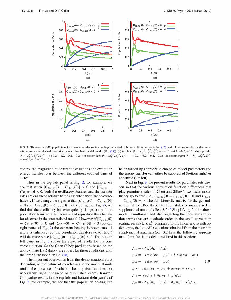
FIG. 2. Three state FMO populations for site energy-electronic coupling correlated bath model Hamiltonian in Eq. (16). Solid lines are results for the modelwith correlations, dashed lines give independent bath model results (Eq. (18)): (a) top left: (k1,2

1 , k1,22 , k

2,32 , k

2,33 ) = (−0.2,+0.2,−0.2,+0.2). (b) top right:

(k1,21 , k

1,22 , k

2,32 , k

2,33 ) = (+0.2,−0.2,+0.2,−0.2). (c) bottom left: (k1,2

1 , k1,22 , k

2,32 , k

2,33 ) = (+0.2,−0.2,−0.2,+0.2). (d) bottom right: (k1,2

1 , k1,22 , k

2,32 , k

2,33 )

= (−0.2,+0.2,+0.2,−0.2).

control the magnitude of coherent oscillations and excitationenergy transfer rates between the different coupled pairs ofstates.

Thus in the top left panel in Fig. 2, for example, wesee that when [C22, 12(0) − C11, 12(0)] > 0 and [C22, 23 −C33, 23(0)] < 0, both the oscillatory features and the transferrates are enhanced relative to the case when there are no corre-lations. If we change the signs so that [C22, 12(0) − C11, 12(0)]< 0 and [C22, 23(0) − C33, 23(0)] > 0 (top right of Fig. 2), wefind that the oscillatory behavior quickly damps out and thepopulation transfer rates decrease and reproduce their behav-ior observed in the uncorrelated model. However, if [C22, 12(0)− C11, 12(0)] > 0 and [C22, 12(0) − C33, 12(0)] > 0 (bottomright panel of Fig. 2) the coherent beating between states 1and 2 is enhanced, but the population transfer rate to state 3will decrease since [C22, 23(0) − C33, 23(0)] > 0. The bottomleft panel in Fig. 2 shows the expected results for the con-verse situation. So the Chen-Silbey predictions based on theapproximate HSR theory are robust for these conditions withthe three state model in Eq. (16).

The important observation from this demonstration is thatdepending on the nature of correlations in the model Hamil-tonian the presence of coherent beating features does notnecessarily signal enhanced or diminished energy transfer.Comparing results in the top left and bottom right panels ofFig. 2, for example, we see that the population beating can

be enhanced by appropriate choice of model parameters andthe energy transfer can either be suppressed (bottom right) orenhanced (top left).

Next in Fig. 3, we present results for parameter sets cho-sen so that the various correlation function differences thatplay prominent roles in Chen and Silbey’s two state modeltheory go to zero, i.e., C22, 12(0) − C11, 12(0) = 0 and C22, 23

− C33, 23(0) = 0. The full Liouville matrix for the general-ization of the HSR theory to three states is summarized insupplemental materials Sec. S.2.39 Simplifying for the abovemodel Hamiltonian and also neglecting the correlation func-tion terms that are quadratic order in the small correlationscaling parameters, k

ij

i compared to the linear and zeroth or-der terms, the Liouville equations obtained from the matrix insupplemental materials Sec. S.2 have the following approxi-mate form for the model considered in this section:

ρ11 = i�12(ρ12 − ρ21)

ρ22 = −i�12(ρ12 − ρ21) + i�23(ρ23 − ρ32)

ρ33 = −i�23(ρ23 − ρ32) (19)

ρ12 = i�12(ρ11 − ρ22) + η12ρ12 + χ23ρ13

ρ13 = χ23ρ12 + η13ρ13 + χ∗12ρ23

ρ23 = i�23(ρ22 − ρ33) − η23ρ23 + χ∗12ρ13,



0

0.2

0.4

0.6

0.8

1

0 0.2 0.4

(a) (b)

0.6 0.8 1

Pop

ulat

ion

of B

chls

t (ps)

C22,12(0) + C11,12(0) > 0

C22,23(0) + C33,23(0) < 0

123

0

0.2

0.4

0.6

0.8

1

0 0.2 0.4 0.6 0.8 1

Pop

ulat

ion

of B

chls

t (ps)

C22,12(0) + C11,12(0) < 0

C22,23(0) + C33,23(0) < 0

123

FIG. 3. Same as Fig. 2 except parameters are chosen so that now C22, 12 − C11, 12 = 0 and C22, 12 − C33, 12 = 0 and the correlation function sums have thenonzero values indicated. Again, solid lines are results for model with correlations, and dashed lines are independent bath model results. Parameters used are:(a) left: (k1,2

1 , k1,22 , k

2,32 , k

2,33 ) = (+0.2,+0.2,−0.2,−0.2). (b) right: (k1,2

1 , k1,22 , k

2,32 , k

2,33 ) = (−0.2,−0.2,−0.2,−0.2).

where χ ij = [i�ij − (γ ii, ij + γ jj, ij)], ηij = [i(εi − εj) −(γ ii, ii + γ jj, jj)] and the other off-diagonal density matrix ele-ment equations of motion are obtained by complex conjuga-tion. The important observation here is that the key quanti-ties controlling the relaxation with this parameterization arecorrelation function sums involving the site energy-inter-sitecoupling fluctuation correlation functions that appear in theparameters χ ij, i.e., Cii, ij(0) + Cjj, ij(0) = γ ii, ij + γ jj, ij.

For the results presented in Fig. 3 we have chosen the|ki,j

i | = 0.2, which means that the zero time magnitudes of thesite-inter-site coupling correlations functions, Cii, ij are about5 times larger than the inter-site coupling-inter-site couplingcorrelation functions, e.g., Cij, jk, so ignoring these terms asin the above equations is appropriate. Under these circum-stances the correlation function sum quantities, e.g., Cii, ij(0)+ Cjj, ij(0), are observed in Fig. 3 to have controlling influenceon the population relaxation dynamics. In the right panel ofFig. 3, for example, we see that having both correlation func-tion sums negative has little influence on the population re-laxation dynamics though it does cause more rapid dampingof the coherent population oscillation compared to the uncor-related situation. Making the sign of [C22, 12(0) + C11, 12(0)]> 0 but keeping [C22, 23(0) + C22, 23(0)] < 0 is seen to enhancethe rate of energy transfer from state 1 to state 3, leaving thestate 2 population dynamics essentially unchanged. Note theHamiltonian for this model is constructed so that the directcoupling between states 1 and 3 is small and so the energymust be transferred through the intermediate state 2. Gener-ally for this type of model we see that initial state 1 and inter-mediate state 2 show short time coherent oscillation of theirpopulations. The terminal state 3, which is fed by coupling tointermediate state 2, on the other hand, shows essentially noremnant of the initial coherence between the 1 and 2 dimersystem and we observe incoherent exponential growth in thepopulation of terminal state 3.

The final class of model Hamiltonians that we considerin this paper has, in addition to the baths describing the inde-pendent relaxation of the three sites, further groups of inde-pendent bath oscillators that interact with the inter-site elec-tronic coupling terms to include correlation in the fluctuations

of these couplings. The first such model we consider includesa set of bath oscillators that interact with the inter-site elec-tronic coupling terms in such a way as to account for corre-lation in the fluctuations of coupling between sites 1–2 andsites 2–3. The various terms included in this model Hamilto-nian are thus detailed in equations below:

Hb =3∑

α=1

n(α)∑l=1

1

2

[p

(α2)l + ω

(α2)l q

(α2)l

](20)

+n(123)∑l=1

1

2

[p

(123)2l + ω

(123)2l q

(123)2l

],

Hs−b =n(1)∑l=1

c(1)l q

(1)l |1〉〈1| +

n(2)∑l=1

c(2)l q

(2)l |2〉〈2|

+n(3)∑l=1

c(3)l q

(3)l |3〉〈3| (21)

+n(123)∑l=1

k1,2123c

(123)l q

(123)l [|1〉〈2| + |2〉〈1|]

+n(123)∑l=1

k2,3123c

(123)l q

(123)l [|2〉〈3| + |3〉〈2|],

and the fluctuations in the inter-site coupling-inter-site cou-pling terms in this model are described by the correlationfunctions,

C12,12(t) = kBT

n(123)∑l=1

(k

1,2123

)2 c(123)2l

ω(123)2l

cos(ω

(123)l t)

C12,23(t) = kBT

n(123)∑l=1

k1,2123k

2,3123

c(123)2l

ω(123)2l

cos(ω

(123)l t)

C23,23(t) = kBT

n(123)∑l=1

(k

2,3123

)2 c(123)2l

ω(123)2l

cos(ω

(123)l t). (22)



0.0

0.2

0.4

0.6

0.8

0 0.2 0.4 0.6 0.8 1

ρ 33(

τ)

t (ps)

(c)

0.0

0.2

0.4

0.6

0.8

ρ 22(

t)

(b)

0.0

0.2

0.4

0.6

0.8

1.0

ρ 11(

t)

(a) C12,12=C23,23>0,C12,23>0C12,12=C23,23>0,C12,23=0C12,12=C23,23>0,C12,23<0C12,12=C23,23=0,C12,23=0

0.00

0.10

0.20

0.30

0.40

0 0.2 0.4 0.6 0.8 1

ρ 23(

τ)

t (ps)

(c)0.00

0.10

0.20

0.30

0.40

ρ 13(

t)

(b)0.00

0.10

0.20

0.30

0.40

ρ 12(

t)

(a) C12,12=C23,23>0,C12,23>0C12,12=C23,23>0,C12,23=0C12,12=C23,23>0,C12,23<0C12,12=C23,23=0,C12,23=0

FIG. 4. Comparison of density matrix dynamics results for various models that include correlated fluctuations in electronic coupling between chromophores.Left panel shows state populations, while right panel displays off-diagonal or coherence density matrix elements computed in the site basis. The magenta curvesgive results computed for the original independent bath model, the green curves are computed using the model Hamiltonian with two independent electroniccoupling baths in Eq. (24). The red and blue curves are computed with the common coupling bath model determined by the Hamiltonian in Eq. (21). In thiscase the magnitudes of the rescaling factors (the ks in these equations) are 0.4, and the signs are chosen to give the indicated signs of the correlation functions,e.g., C12, 23, etc.

For comparison, in the final model we consider here, weremove the terms that correlate fluctuations in coupling be-tween the two dimers, and incorporate independent baths de-scribing uncorrelated fluctuations in the independent dimercouplings. Thus, this final model is described by the follow-ing Hamiltonian terms:

Hb =3∑

α=1

n(α)∑l=1

1

2

[p

(α)2l + ω

(α)2l q

(α)2l

](23)

+n(12)∑l=1

1

2

[p

(12)2l + ω

(12)2l q

(12)2l

]

+n(23)∑l=1

1

2

[p

(23)2l + ω

(23)2l q

(23)2l

],

Hs−b =n(1)∑l=1

c(1)l q

(1)l |1〉〈1| +

n(2)∑l=1

c(2)l q

(2)l |2〉〈2| (24)

+n(3)∑l=1

c(3)l q

(3)l |3〉〈3|

+n(12)∑l=1

k1,2c(12)l q

(12)l [|1〉〈2| + |2〉〈1|]

+n(23)∑l=1

k2,3c(23)l q

(23)l [|2〉〈3| + |3〉〈2|],

and the non-vanishing inter-site coupling correlation func-tions for this model are,

C12,12(t) = kBT

n(12)∑l=1

(k1,2)2 c

(12)2l

ω(12)2l

cos(ω(12)l t) (25)

C23,23(t) = kBT

n(23)∑l=1

(k2,3)2 c

(23)2l

ω(23)2l

cos(ω(23)l t).

For these last two models, because the relevant correla-tion functions depend only quadratically on the bath interac-tion correlation rescaling parameters (the ks) we have set theirmagnitudes to be |k| = 0.4 so k2 ∼ 0.2, which makes theseterms in this model of comparable magnitude to the domi-nant linear terms in the previous model that incorporated site



energy-inter-site coupling correlations (whose magnitude weset by choosing |k| = 0.2 for these earlier models).

The evolution of the populations and coherence densitymatrix elements for the models outlined above are comparedin Fig. 4. The results presented here show that in the ab-sence of correlation in inter-site electronic coupling fluctua-tions (magenta curves) oscillations in the ρ12 coherence per-sist out to about 400 fs (the bare model was fit to reproducethis experimental observation) and in this situation the energytransfer rate as measured by the growth in population, ρ33, isslowest. Adding correlated inter-site coupling fluctuations sothat C12, 12 = C23, 23 > 0 (red, green, and blue curves) gener-ally increases the energy transfer rate, but also damps out theoscillations in coherence more rapidly. The overall magnitudeof the increase in energy transfer rate is observed to dependon the strength and sign of the inter-dimer coupling fluctua-tion correlation function, C12, 23, with the largest increase inenergy transfer rate occurring when C12, 23 < 0, and in thiscase the transfer rate is nearly double that of when there areno correlations in inter-site couplings.

From Fig. 4 we see that in all cases including fluctua-tions in the electronic coupling matrix elements, whether theyinvolve correlation, or not, increase the energy transfer rateand reduce the coherence time. In order to recover the experi-mentally observed long lived coherence relaxation time scalewith a model that includes environment induced fluctuationsin electronic coupling, the magnitude of the electronic cou-pling in the bare model system Hamiltonian (e.g., the �

(0)i,j in

Eq. (5)) would need to be increased. Interestingly, the coher-ence relaxation time observed with the different treatments ofcorrelated fluctuations in Fig. 4 seem to be largely indepen-dent of the nature of the correlation.

III. CONCLUSIONS

In this paper, we have employed accurate semiclassi-cal quantum dynamics methods that can reliably treat gen-eral models for dissipative open quantum system-bath dynam-ics to explore the characteristics of excitation energy transferprocesses in a number of general paradigms for incorporat-ing the effects of various types of correlated fluctuations inmodel system parameters driven by interactions with the en-vironment. While the calculations we report here have beenfocused on models for excitation energy transfer in photo-synthetic light harvesting systems, due to the availability ofhighly detailed recent nonlinear optical spectroscopy stud-ies on these systems that report the timescales for the com-petition between coherent and incoherent dynamics in theseprocesses, our approach should be generally applicable tostudy models for similar quantum processes that may playimportant roles in, for example, electron transport in nano-structured complex systems where donors and acceptors (ofeither excitation energy or electrons) are embedded with suf-ficient density, in an environment capable of fluctuating ona range of length-scales including those characteristic of theinter donor-acceptor interactions that are responsible for thetransport processes of interest.

While the models we have studied here have been ofa fairly standard multi-state system-bi-linearly coupled har-

monic bath form, the semi-classical quantum dynamics meth-ods that we have developed, and employed for these stud-ies are generally applicable to more complex models and donot require the use of Markovian, secular or high tempera-ture approximations, or even the use of perturbation theory.As such the general findings of our studies provide an impor-tant benchmark for testing approximate approaches to under-standing the effects of correlated fluctuations on dissipativequantum dynamics in complex systems.

To summarize the findings of these studies, our main fo-cus here has been on building model Hamiltonians that cancapture how environmental modes might modulate, in a cor-related way, the off-diagonal couplings between electronicstates in which excitation energy is localized at different in-teracting sites. Appendix presents some results obtained formore standard models7–9, 22, 26 that incorporate correlated fluc-tuations in diagonal site excitation energies. For these mod-els we generally find that as the strength of correlation is in-creased, the quantum coherent oscillation in populations canbe enhanced, but with such models, in this strongly corre-lated regime, the energy transfer rate will be slowed downsignificantly. Thus enhanced coherent dynamics with corre-lated site energy fluctuations causes slower energy transferwith these sorts of models. In contrast, in the main body ofthe paper we show that with more general model Hamiltoni-ans that incorporate the effects of correlated fluctuations inthe off-diagonal electronic couplings (as well as in the diago-nal site energies) the range of energy transport behaviors thatcan be addressed are much more varied and interesting. Thus,for example, the relative sign and strength of different typesof correlations can be adjusted to give situations in which wesimultaneously enhance the population beating signatures ofquantum coherence and increase the energy transfer rate be-tween donor and acceptor sites whose off-diagonal electroniccouplings are correlated appropriately by environmental fluc-tuations. In fact, a wide range of possibilities open up withmodel Hamiltonians with this type of flexibility.

Several theoretical groups11–15 have begun exploring de-tailed microscopic simulation models looking for differenttypes of environment driven correlated fluctuations in chro-mophore electronic properties. The ubiquitous finding fromthe various photosynthetic energy transfer systems studiedso far is that fluctuations in site energies seem to be suchthat on average they are uncorrelated. However, there is ev-idence that the fluctuations in electronic couplings betweendifferent pairs of chromophores show correlation. It thusseems unlikely that the situation in real systems is as restric-tive as the simple correlated site energy fluctuation modelwould suggest and more work both from the experimentaland theoretical directions to elucidate the nature of such cor-relations and their influence on dynamics needs to be donewith the aim to begin to design environments that can beself-assembled to take advantage of these correlations as amechanism to control energy and charge transport in fluctuat-ing nano-structured environments. Powerful new approaches,like quantum process tomography,52 are in principle capableof combining advanced multidimensional electronic spectro-scopies with quantum dynamical theoretical methods to en-able extraction of the detailed quantum information necessary



to build more realistic models that can accurately parameter-ize the more general classes of models for correlated fluctua-tions that we have begun exploring in this paper.

ACKNOWLEDGMENTS

We would like to dedicate this publication to the memoryof Bob Silbey. He, and his work in this area, will continue tobe an inspiration to us, and indeed the whole field. We grate-fully acknowledge support for this research from the NationalScience Foundation (NSF) under Grant No. CHE-0911635.D.F.C. acknowledges the support of his Stokes Professorshipin Nanobiophysics and Principle Investigator Grant No. 10/IN.1 / I3033 from Science Foundation Ireland. P.H. appreci-ates discussions with Sara Bonella and Xin Chen. We alsoacknowledge a grant of supercomputer time from the BostonUniversity Office of Information Technology and ScientificComputing and Visualization.

APPENDIX A: QUANTUM DYNAMICS OFCORRELATED SITE ENERGY FLUCTUATION MODELS

In this appendix, we present the results of our quan-tum dynamics calculations on the model that was fit to re-produce the experimental data on excitation energy transferbetween the accessory bacteriochlorophyll (Bchl or B) andbacteriopheophytin (BPhy or H) chromophores embedded inthe transmembrane protein scaffolding near the reaction cen-ter of Rhodobacter sphaeroides as reported by Lee et al.1 Tofit the experimental spectral dynamics reasonably, these au-thors found that they could assume the fluctuations in the Band H site energies were strongly correlated, giving rise to in-phase energy fluctuations that preserved coherence.1 It wasfound that strong electronic coupling, which could also leadto longer lived coherence, would not give a reasonable fit toexperimental data.1 These authors did not consider the gener-alized model that allows for inter-site coupling-inter-site cou-pling correlations explored in the present work.

The total Hamiltonian for this experimentally fittedmodel based on correlated site energy fluctuations is de-scribed by four terms,

H = Hs + Hs−b + Hb + Hbrown (A1)

Here the two state electronic subsystem part of the Hamilto-nian is given in Eq. (2), and Hb and Hs−b are the bath andsystem-bath interaction terms, respectively. The term Hbrown

describes the vibrations of a damped protein mode (a Brown-ian oscillator) that was observed to modulate the experimen-tal signals. The detailed treatment of this Brownian modewill be outlined later. In the calculations outlined here wehave considered two different models for the bath and system-bath interaction terms based on different descriptions for howenvironmental effects might cause correlation in site energyfluctuations.

First, the common bath model9, 24 assumes that chro-mophores H and B have their own harmonic baths, and wealso introduce a set of modes that are “common” to both chro-mophores so the common bath model Hamiltonian has the

form,

H comb =

∑α=H,B

n(α)∑l=1

1

2

[p

(α)2l + ω

(α)2l q

(α)2l

](A2)

+n

(HB)com∑

m=1

1

2

[P (HB)2

m + �(H,B)2m Q(HB)2

m

]

H coms−b =

⎡⎣n(H )∑

l=1

c(H )l q

(H )l +

n(HB)com∑

m=1

C(H )m Q(HB)

m

⎤⎦ |H 〉〈H |

+⎡⎣ n(B)∑

l=1

c(B)l q

(B)l +

n(HB)com∑

m=1

C(B)m Q(HB)

m

⎤⎦ |B〉〈B|.

The second bath model is the so-called cross couplingmodel23 that again includes different bath modes for the H andB chromophores. With the cross coupling model, however,there are coefficients xBH, for example, that scale the strengthof coupling of the H bath modes to the B chromophore andvisa versa, so the bath Hamiltonian terms for this cross cou-pling model have the following form:

H crossb =

∑α=H,B

n(α)∑l=1

1

2

[p

(α)2l + ω

(α)2l q

(α)2l

]

H crosss−b =

{xHH

n(H )∑l=1

c(H )l q

(H )l

+ xHB

n(B)∑l=1

c(B)l q

(B)l

}|H 〉〈H |

+{

xBH

n(H )∑l=1

c(H )l q

(H )l

+ xBB

n(B)∑l=1

c(B)l q

(B)l

}|B〉〈B|, (A3)

In the common bath model q(H )l , q

(B)l represent the lth

independent bath oscillator that couple to the |H〉 or |B〉 states,respectively, with coupling strengths c

(H )l and c

(B)l . The mth

common bath oscillator mode Q(HB)m couples to both the |H〉

and |B〉 states simultaneously. With this model, these commonbath modes give rise to correlated energy level fluctuationswhen the common bath coupling constants C(H )

m and C(B)m are

not zero.In the cross coupling model, the correlation is introduced

by making the energy of a given chromophore depend bothon its own bath coordinates and on the bath coordinates as-sociated with another chromophore’s bath. In this model, forexample, q

(B)l is the lth mode that would normally be inde-

pendently coupled to chromophore B with coupling strengthc

(B)l . With the cross coupling model, however, by introducing

the cross coupling, this mode is also coupled to chromophorestate |H〉 with rescaled cross correlation factor xHB.

The approach employed in fitting the experimental data1

assumes a model for the correlated fluctuations in site



excitation energies of the B and H chromophores based onthe strength of correlation, a, specified by the following rela-tionship between the different spectral densities

j (HB)(ω) = |a|√

j(H )tot j

(B)tot (ω), (A4)

where the spectral densities, for example, j (H )tot (ω) and j(HB)(ω)

determine the site energy correlation function, CHH, HH(t), andcross-correlation function, CHH, BB(t), respectively. The valueof the correlation strength defined in this way obtained fromthe fit to experimental data1 is a = 0.9.

In order to connect this assumed relationship be-tween spectral densities and the model Hamiltoniansoutlined above, our analysis starts by using the modelsto compute these various correlation functions definedas follows: CHH,BB(t) = 〈〈H |Hs−b(t)|H 〉〈B|Hs−b(0)|B〉〉= 〈UHH (t)UBB(0)〉, the cross-correlation function correlatesfluctuations in site energies of the different chromophores,and CHH, HH(t) = 〈UHH(t)UHH(0)〉, is the regular site excitationenergy fluctuation correlation function. The Hamiltoniansfor the different bi-linear system-harmonic bath interactionmodels given above can be used to compute exact expressionsfor these various correlation functions written in terms of thespectral densities. The relationship in Eq. (A4) is thus usedto give a consistent specification of the model Hamiltonianparameters.

For the common bath model, for example, the siteexcitation energy fluctuation correlation function, e.g.,CHH, HH(t), will be determined by the total spectral den-sity, j

(H )tot , arising from all influences of the protein en-

vironment on chromophore H. From Eq. (A2) j(H )tot con-

tains contributions from both the independent bath modesof this chromophore, q

(H )l , and from the common bath

modes, Q(HB)m . The general relationship between the spec-

tral density and the correlation function is: CHH,HH (t)= ¯

π

∫∞0 dωj

(H )tot (ω)[coth(¯βω/2) cos(ωt) − i sin(ωt)].

In Ref. 1 a simple ohmic with Lorentzian truncationform, j

(α)tot (ω) = 2λ(α)(ωτc

α)/[(ωτcα)2 + 1], (with α = H or

B) is assumed for this total spectral density, and the follow-ing values of reorganization energy and relaxation time: λH

= 50 cm−1 and λB = 80 cm−1, τ cH = τ c

B = 60 fs, are used.This model also incorporates static disorder for each of thesite energies with δH = δB = 20 cm−1, however, for simplic-ity we neglect the contribution of static disorder in the cross-correlation function as it has only a minor effect on the dy-namics for this system. Thus, in the limit where ¯→ 0, thisexperimentally determined total spectral density for the com-mon bath model can be related through the following classicalresult to the site energy fluctuation correlation function:53

CcomHH,HH (t) = kBT

π

∫ ∞

0dω

j(H )tot (ω)

ωcos(ωt)

= kBT

n(H )∑l=1

c(H )2l

ω(H )2l

cos(ω

(H )l t)

+ kBT

n(HB)com∑

m=1

C(H )2m

�(HB)2m

cos(�(HB)

m t)

= kBT

π

∫ ∞

0dω

j(H )ind (ω)

ωcos(ωt)

+ kBT

π

∫ ∞

0dω

j (H )com(ω)

ωcos(ωt), (A5)

with similar structure of CcomBB,BB(t), and here

we have defined the component, “independent”and “common” bath spectral densities as, respec-tively: j

(H )ind (ω) = π

2

∑n(H )

l=1 (c(H )2l /ω

(H )l )δ(ω − ω

(H )l ) and

j (H )com(ω) = π

2

∑n(HB)com

m=1 (C(H )2m /�(HB)

m )δ(ω − �(HB)m ). From the

above result, for this common bath model, we find that

j(H )tot (ω) = j

(H )ind (ω) + j (H )

com(ω), (A6)

and with these definitions j(H )ind (ω), j (H )

com(ω), and j(H )tot (ω) are

all positive definite. The single parameter relationship under-lying the fitting form assumed in Eq. (A4) can be relatedto the common bath model parameterization by identifyingthe correlation strength (absolute value of a) as the frac-tion of the total spectral density represented by the commonbath component, i.e., |a| = j (H )

com(ω)/j (H )tot (ω) and, dividing the

above result by j(H )tot (ω), gives 1 − |a| = j

(H )ind (ω)/j (H )

tot (ω). Sowith this simplest of interpretations the spectral densities allhave the same frequency dependence (shape) as j

(H )tot (ω) but

their relative strengths are scaled by |a|, thus for examplej (H )com(ω) = |a|j (H )

tot (ω), etc. The model underlying Eq. (A4)supposes that the same scaling factor, a, also relates the vari-ous spectral densities of the bath of chromophore B to its totalspectral density, so e.g., j (B)

com(ω) = |a|j (B)tot (ω).

Also due to the introduction of the common couplingmodes in the common bath model, the cross-correlation func-tion Ccom

HH,BB(t) is non-zero and has the form,

CcomHH,BB = kBT

π

∫ ∞

0dω

j (HB)com (ω)

ωcos(ωt)

= kBT

n(HB)com∑

m=1

C(H )m C(B)

m

�(HB)2m

cos(�(HB)

m t), (A7)

where we have defined the common bath spectral density as

j (HB)com (ω) = π

2

n(HB)com∑

m=1

(C(H )

m C(B)m /�(HB)

m

)δ(ω − �(HB)

m

),

(A8)which, depending on the relative signs of the system-commonbath coupling constants C(H )

m and C(B)m could either be pos-

itive (correlated common bath for H and B) or negative(anti-correlated).

Finally, from the definitions in Eqs. (A5) and (A7), theheights of each δ-distribution at a given common bath modefrequency require that the common bath spectral densitiessatisfy the following equality (j (HB)

com (ω))2=j (H )com(ω)j (B)

com(ω).Substituting the expressions obtained above, i.e., j (H )

com(ω)= |a|j (H )

tot (ω), and j (B)com(ω) = |a|j (B)

tot (ω) we arrive at theassumed spectral density relationship within the com-mon bath model Hamiltonian formulation: j (HB)

com (ω)

= |a|√

j(H )tot (ω)j (B)

tot (ω), giving a useful physical interpretationfor the strength of correlation |a|.



For cross coupling model, these correlation functions canbe expressed as

CcrossHH,HH (t) = kBT

π

∫ ∞

0dω

cos(ωt)

ω

[x2

HHj(H )tot (ω)

+ x2HBj

(B)tot (ω)

]

= kBT

[n(H )∑l=1

x2HH

c(H )2l

ω(H )2l

cos(ω(H )l t)

+n(B)∑l=1

x2HB

c(B)2l

ω(B)2l

cos(ω

(B)l t)]

CcrossHH,BB(t) = kBT

π

∫ ∞

0dω

cos(ωt)

ω

[xHHxBH j

(H )tot (ω)

+ xHBx2BBj

(B)tot (ω)

]

= kBT

[n(H )∑l=1

xHH xBH

c(H )2l

ω(H )2l

cos(ω(H )l t)

+n(B)∑l=1

xHBxBB

c(B)2l

ω(B)2l

cos(ω(B)l t)

]. (A9)

These expressions can be rewritten using short handdefinitions of CHH and CHB, giving the following sys-tem of equations: CHH = x2

HHCHH + x2HBCBB , CBB

= x2BH CHH + x2

BBCBB , CHB = xHHxBHCHH + xHBxBBCBB,CBH = xBHxHHCHH + xBBxHBCBB. Writing each correlationfunction in terms of the total spectral densities and substitut-ing the Lorentzian truncated ohmic forms with the appropriatecombination of reorganization energies, λK obtained usingEq. (A4), we obtain: λH = x2

HHλH + x2HBλB , λB

= x2BH λH + x2

BBλB , a√

λHλB = xHHxBH λH + xHBxBBλB ,a√

λBλH = xBH xHHλH + xBBxHBλB , and the solution is23

(xHH xHB

xBH xBB

)= 1√

1 + ζ 2

(1 λH

λB

1/2ζ

λB

λH

1/2ζ 1

),(A10)

where a = 2ζ

1+ζ 2 . We can see that although CHB = CBH is re-quired, it is not necessary for xBH = xHB, which means the xmatrix could be non-Hermitian.

The calculation results reported below with these differ-ent models have T = 180 K. We find that the common bathmodel and cross coupling model for this two state systemgive identical descriptions of the exciton dynamics due to theequivalence of the correlation functions with these models.

As mentioned earlier, the model Hamiltonian in Eq. (A1)developed by Lee et al.1 includes an explicit additional modethat modulates the excitation energy of the H state so as tocapture the low frequency oscillation observed in the exper-imental signal. The behavior of the signal suggests that thismode exhibits damped oscillatory motion and so it is modeledas a Brownian mode, Qb, with frequency, �b, that couples tothe population of state |H〉 with bi-linear coupling strengthCb, as well as to its own dissipative bath of harmonic oscilla-tors with coordinates q

(b)i . Thus this Brownian oscillator term,

Hbrown, in Eq. (A1) has the following form:

Hbrown = 1

2

[P 2

b + �2bQ

2b

]+ CbQb|H 〉〈H | (A11)

+nb∑i=1

{1

2

[p

(b)2i + ω

(b)2i q

(b)2i

]

+[c

(b)i q

(b)i Qb + c

(b)2i Q2

b

2ω(b)2i

]|H 〉〈H |

}.

The physical origin of this mode is a low frequency collec-tive protein vibration. Here Cb = √

2�bS�b (with ¯ = 1),�b = 250 cm−1 is the frequency of the Brownian vibrationalmode and S = 0.4 is the Huang-Rhys factor. The couplingstrength, c

(b)i , between the dissipative bath mode qi and the

Brownian mode, is sampled from the spectral density: jb(ω)= γωexp −ω/�, where the γ=50 cm−1 is the damping con-stant of the bath for the Brownian mode and � = 100 cm−1

is the cutoff frequency for this dissipative bath.In the calculations, we explored three different ini-

tial conditions for the Brownian mode: (1) The tra-jectories have an initial phase shift φ = 0.28, whichmeans that the initial condition has either Qb sam-pled from T rPb

ρw ∼ tanh(β�b/2)e−[tanh(β�b/2)�b][(�2bQ

2b/2)],

i.e., the momentum integrated Wigner density, and Pb

= tan φQb or; (2) Qb =√

1�b

cos φ and Pb = √�b sin φ, or

finally; (3) the thermal distribution (Wigner density), ρw

= tanh(β�b/2)e−[tanh(β�b2)/�b][P 2b /2+(�2

bQ2b/2)] was used to

sample both Qb and Pb. With this thermal sampling we av-erage over a uniform relative phase distribution.

According to Garg et al.,44 this Brownian model canbe expressed as an equivalent system-bath model, H trans

brown,through a coordinate transformation giving,

H transbrown =

n∑i=1

{1

2

[p

(b)2i + ω

(b)2i q

(b)2i

]+ c(b)i q

(b)i |H 〉〈H |

},

where qi are the transformed coordinate (containing both Qb

and qi) and they form a bath with a Brownian spectral densityfrom which ci is sampled:

jbrown(ω) = C2bγω

(ω2 − �2b)

2 + γ 2ω2= 2S�3

bγω

(ω2 − �2b)

2 + γ 2ω

= 2λb�2bγω

(ω2 − �2b)

2 + γ 2ω2, (A12)

where jbrown(ω) = π2

∑ni

c(b)2i

ω(b)i

δ(ω − ω(b)i ). Here we define the

solvent reorganization energy as λb = S�b. In the case whereγ 2�b, the Brownian spectral density can be rewritten asj (ω) = 2λb�bω

ω2+�2b

which is the Debye cutoff ohmic spectral den-

sity, with �b = �2b/γ (and τ b = 1/�b is the solvent response

time). This is the so-called over-damped Brownian oscilla-tor model,45 which is a special case of the Brownian model.In the reaction center application, the explicit Brownian os-cillator does not obey this relation due the parameters beingappropriate for the under-damped limit with γ < �b. In the



reaction center model, due to the initial phase shift of theBrownian oscillator coordinate, it is better to use the Brow-nian oscillator model rather than the transformed form sincethe non-thermal initial condition is hard to transform for theH brown

trans representation. Alternatively, we can set up the Brow-nian oscillator model by integrating out the dissipative bathdegrees of freedoms giving an influence functional form forthe Brownian mode, which can be modeled using a quantumLangevin like dynamics.46 Here, however, we simply use theILDM scheme35 to explicitly propagate every degree of free-dom for the bath, including the dissipative bath oscillatorscoupled to Brownian mode.

The top panels of Fig. 5 present the site population ρHH

for the initial condition of the Brownian oscillator with phaseshift φ = 0.28 using initial conditions (1) and (2). These up-per panels also compare results with, or with out the Brow-nian mode, which is seen to provide simply a low frequencymodulation on the high frequency electronic population os-cillation. From the left and right panels we see that for themodel without the additional Brownian mode and its dissi-pative bath, the population simply oscillates with a periodof about 40 fs. This frequency is determined by electronicproperties (site energy difference and electronic coupling,

which determined the behavior of |H〉 as |aH(t)|2 ∼ 1 −4cos 2θsin 2θsin 2(δt/¯) where δ = 1

2

√[εH − εB]2 + 4�2

H,B

and θ = 12 {π

2 − sin−1([εH − εB]/2δ)} (Ref. 36)) and agreeswith the behavior observed as the fine structure in theexperiment.1 If we include the H brown component, it gives themodulating envelop with a slower oscillation frequency witha period of about 125 fs corresponding to the 250 cm−1 Brow-nian oscillator frequency. This is the major beating frequencyobserved in the experimental results1 and originates fromsome protein environmental vibrational degree of freedom be-ing excited during the experiment. Also we observe that theelectronic beating damps out at about 120 fs if no bath corre-lation effects are included (a = 0). This is much shorter thanthe experimentally observed decoherence time scale around300 fs, suggesting the importance of correlated bath motions.Thus, one way to capture the experimentally observed longerdecoherence time, is to include correlated fluctuations in siteenergies driven by the environment. However, such correlatedsite energy fluctuations have not been observed in detailedsimulations. The main text of this paper suggests that corre-lations in off-diagonal couplings, that have been observed inmodel system studies, may lead to long coherence times with

0.3

0.4

0.5

0.6

0.7

0.8

0.9

1

0

(a) (b)

(c) (d)

0.05 0.1 0.15 0.2

Pop

ulat

ion

of H

t (ps)

w/o B mode,a=0.0w/o B mode,a=0.9

w B mode,a=0.0w B mode,a=0.9

0.3

0.4

0.5

0.6

0.7

0.8

0.9

1

0 0.05 0.1 0.15 0.2

Pop

ulat

ion

of H

t (ps)

0

0.2

0.4

0.6

0.8

1

0 0.05 0.1 0.15 0.2

Pop

ulat

ion

t (ps)

H brownian modelH trans-brown model

B brownian modelB trans-brow model

0

0.2

0.4

0.6

0.8

1

0 0.05 0.1 0.15 0.2

Pop

ulat

ion

t (ps)

H brownian modelH trans-brown model

B brownian modelB trans-brow model

FIG. 5. Top panels: Population of H at T = 180 K with initial excitation at H. The site disorders are 20 cm−1 for both B and H. Left panel: Qb sampled

from Wigner density T rPbρw ∼ tanh(β�b/2)e[− tanh(β�b/2)/�b ][(�2

bQ2

b/2)] and Pb = tan φQb. Right panel: Qb =

√1

�bcos φ, Pb = √

�b sin φ. Bottom panels:

Population of H and B for initial condition which has the thermal distribution of the Brownian mode, i.e., ρw = tanh(β�b/2)e−[tanh(β�b/2)�b ][P 2b/2+(�2

bQ2

b/2)].

Left panel is the situation for a = 0 and right for a = 0.9. Also the results for both Brownian oscillator model and system-bath coupling model with a Brownianspectral density are presented. Red and greed curves are H and B populations obtained from the Brownian oscillator model, and blue and magenta curves are Hand B populations obtained from the system-bath model.



-0.4

-0.2

0

0.2

0.4

0.6

0.8

1

0 0.05 0.1 0.15

(a) (b)

(c) (d)

0.2 0.25 0.3-0.4

-0.2

0

0.2

0.4

0.6

0.8

1

0 0.05 0.1 0.15 0.2 0.25 0.3

-0.4

-0.2

0

0.2

0.4

0.6

0.8

1

0 0.05 0.1 0.15 0.2 0.25 0.3-0.4

-0.2

0

0.2

0.4

0.6

0.8

1

0 0.05 0.1 0.15 0.2 0.25 0.3

FIG. 6. Dynamics of the reaction center model that ignores the H brown part of the Hamiltonian. Initially the excitation is localized at state H, T = 180 K. Thetime axis in this figure is given in picoseconds. Top panels: a = 0, bottom panels: a = 0.9. Left panels give results in the site basis set (|H〉 and |B〉): ρHH, ρBB,ReρHB, ImρHB are represent by red, green, blue, and magenta curves, respectively. Right panels give results in exciton basis set (| + 〉 and | − 〉), and ρ++,ρ−−, Reρ+−, Imρ+− are represent by red, green, blue, and magenta curves, respectively.

different, perhaps experimentally distinguishable, dynamicalcharacteristics.

The dynamics for Brownian model with the thermal ini-tial distribution (initial condition 3) is presented in bottompanels of Fig. 5 with a = 0 (left) or a = 0.9 (right) spatial cor-relation. Due to the thermal distribution of all degrees of free-dom, the Brownian oscillator model H brownand the system-bath transformed Brownian model H brown

trans with a Brownianspectral density give exactly same reduced density matrix dy-namics. Populations for H and B obtain from both models arecompared.

Finally, in Fig. 6 we use the reaction center model in theabsence of the Brownian mode to explore the effects of corre-lations in site energy fluctuations on decoherence time andthe representation dependence of decoherence terms in thedensity matrix. In the top left panel (a = 0), we see the realpart of the coherence ρHB maintains a finite amplitude at longtimes A detail explanation of this phenomenon is provided inRef. 36 in terms of the overlaps of the time dependent envi-ronmental wave packets. The right panels show the results inexciton basis set (| + 〉 and | − 〉, which are the eigenstatesof HS). Bottom panels compare site and exciton basis results:ρHH − ρBB, 2|ρHB|, ρ++ − ρ−−, 2|ρ+−| are represent by red,green, blue, and magenta curves. One can see that the real partof coherence in site basis which maintains finite value at long

times, vanishes at exciton basis. This is an example of rep-resentation dependence of the “coherence.” The life time ofthe oscillations in the coherence matrix elements is universal(i.e., will always exist in either representation).

1H. Lee, Y.-C. Cheng, and G. R. Fleming, Science 316, 1462 (2007).2E. Collini, C. Y. Wong, K. E. Wilk, P. M. G. Curmi, P. Brumer, andG. D. Scholes, Nature (London) 463, 644 (2010).

3G. S. Engel, T. R. Calhoun, E. L. Read, T.-K. Ahn, T. Mancal, Y.-C. Cheng,R. E. Blankenship, and G. R. Fleming, Nature (London) 446, 782 (2007);G. Panitchayangkoona, D. Hayes, K. A. Fransted, J. R. Caram, E. Harel,J. Wen, R. E. Blankenship, and G. S. Engel, Proc. Natl. Acad. Sci. U.S.A.107, 12766 (2010).

4T. R. Calhoun, N. S. Ginsberg, G. S. Schlau-Cohen, Y.-C. Cheng, M.Ballottari, R. Bassi, and G. R. Fleming, J. Phys. Chem. B 113, 16291(2009).

5A. Ishizaki, T. R. Calhoun, G. S. Schlau-Cohenab, and G. R. Fleming, Phys.Chem. Chem. Phys. 12, 7319 (2010).

6E. Collini and G. D. Scholes, Science 323, 369 (2009).7N. Demirdöven, M. Khalil, and A. Tokmakoff, Phys. Rev. Lett. 89, 237401(2002); J. Phys. Chem. A. 107, 5258 (2003).

8A. Ishizaki and Y. Tanimura, J. Phys. Chem. A 111, 9296 (2007).9A. G. Dijkstra and Y. Tanimura, New J. Phys. 12, 055005 (2010).

10T. Kubar, U. Kleinekathöfer, and M. Elstner, J. Phys. Chem. B 113, 13107(2009).

11C. Olbrich, J. Strümpfer, K. Schulten, and U. Kleinekathöfer, J. Phys.Chem. B 115, 758 (2011).

12S. Shim, P. Rebentrost, S. Valleau, and A. Aspuru-Guzik, Biophys. J. 102,649 (2012).

13C. Olbrich and U. Kleinekathöfer, J. Phys. Chem. B 114, 12427 (2010).


http://dx.doi.org/10.1126/science.1142188

http://dx.doi.org/10.1038/nature08811

http://dx.doi.org/10.1038/nature05678

http://dx.doi.org/10.1073/pnas.1005484107

http://dx.doi.org/10.1021/jp908300c

http://dx.doi.org/10.1039/c003389h

http://dx.doi.org/10.1039/c003389h

http://dx.doi.org/10.1126/science.1164016

http://dx.doi.org/10.1103/PhysRevLett.89.237401

http://dx.doi.org/10.1021/jp0219247

http://dx.doi.org/10.1021/jp072880a

http://dx.doi.org/10.1088/1367-2630/12/5/055005




http://dx.doi.org/10.1016/j.bpj.2011.12.021

http://dx.doi.org/10.1021/jp106542v


14Y. Jing, R. Zheng, H.-X. Li, and Q. Shi, J. Phys. Chem. B 116, 1164 (2012).15C. Curutchet, J. Kongsted, A. Muñoz-Losa, H. Hossein-Nejad, G. D. Sc-

holes, and B. Mennucci, J. Am. Chem. Soc. 133, 3078 (2011).16J. Adolphs and T. Renger, Biophys. J. 91, 2778 (2006).17M. Sarovar, Y.-C. Cheng, and K. B. Whaley, Phys. Rev. E 83, 011906

(2011).18P. Rebentrost, M. Mohseni, and A. Aspuru-Guzik, J. Phys. Chem. B 113,

9942 (2009).19J. Wu, F. Liu, Y. Shen, J. Cao, and R. J. Silbey, New J. Phys. 12, 105012

(2010).20P. Nalbach, J. Eckel, and M. Thorwart, New J. Phys. 12, 065043 (2010);

P. Nalbach and M. Thorwart, New J. Phys. 11, 085001 (2009); New J. Phys.12, 194111 (2010).

21F. Fassioli, A. Nazir, and A. Olaya-Castro, J. Phys. Chem. Lett. 1, 2139(2010); F. Fassioli and A. Olaya-Castro, New J. Phys. 12, 085006 (2010).

22D. Abramavicius and S. Mukamel, J. Chem. Phys. 134, 174504 (2011).23A. Ishizaki and G. R. Fleming, New J. Phys. 12, 055004 (2010).24S. Jang, J. Chem. Phys. 131, 164101 (2009); S. Jang, Y.-C. Cheng,

D. R. Reichman, and J. D. Eaves, J. Chem. Phys. 129, 101104 (2008).25E. Hennebicq, D. Beljonne, C. Curutchet, G. D. Scholes, and R. J. Silbey,

J. Chem. Phys. 130, 214505 (2009).26J. Strümpfer and K. Schulten, J. Chem. Phys. 134, 095102 (2011).27S. Jang, J. Chem. Phys. 127, 174710 (2007).28X. Chen and R. J. Silbey, J. Chem. Phys. 132, 204503 (2010).29S. M. Vlaming and R. J. Silbey, J. Chem. Phys. 136, 055102 (2012).30W. R. Cook, R. D. Coalson and D. G. Evans, J. Phys. Chem. B 113, 11437

(2009).31R. Hernandez and G. A. Voth, Chem. Phys. 223, 243 (1998); J. A. Poulsen,

G. Nyman, and P. J. Rossky, J. Chem. Phys. 119, 12179 (2003);J. A. Poulsen and G. Nyman, J. Phys. Chem. A 108, 8743 (2004);J. A. Poulsen, G. Nyman, and P. J. Rossky, Proc. Natl. Acad. Sci. 102,6709 (2005); Q. Shi and E. Geva, J. Phys. Chem. A 107, 9059 (2003);Q. Shi and E. Geva, J. Chem. Phys. 118, 8173 (2003); Q. Shi and E. Geva,J. Chem. Phys. 119, 9030 (2003); Q. Shi and E. Geva, J. Chem. Phys. 118,7562 (2003).

32Z. Ma and D. F. Coker, J. Chem. Phys. 128, 244108 (2008).33W. H. Miller and C. W. McCurdy, J. Chem. Phys. 69, 5163 (1978);

H. D. Meyer and W. H. Miller, J. Chem. Phys. 70, 3214 (1979); G. Stockand M. Thoss, Phys. Rev. Lett. 78, 578 (1997); M. Thoss and G. Stock,Phys. Rev. A 59, 64 (1999); S. Bonella, and D. F. Coker, J. Chem. Phys.114, 7778 (2001); S. Bonella and D. F. Coker, J. Chem. Phys. 118, 4370(2003).

34P. Huo and D. F. Coker, J. Chem. Phys. 135, 201101 (2011).35E. R. Dunkel, S. Bonella, and D. F. Coker, J. Chem. Phys. 129, 114106

(2008); S. Bonella and D. F. Coker, J. Chem. Phys. 122, 194102 (2005);S. Bonella, D. Montemayor, and D. F. Coker, Proc. Natl. Acad. Sci. U.S.A.102, 6715 (2005).

36P. Huo and D. F. Coker, J. Chem. Phys. 133, 184108 (2010).37P. Huo and D. F. Coker, J. Phys. Chem. Lett. 2, 825 (2011).38S. Jang, M. D. Newton, and R. J. Silbey, Phys. Rev. Lett. 92, 218301 (2004);

Y.-C. Cheng and R. J. Silbey, Phys. Rev. Lett. 96, 028103 (2006); S. Jang,M. D. Netwton, and R. J. Silbey, J. Phys. Chem. B 111, 6807 (2007).

39See supplementary material at http://dx.doi.org/10.1063/1.3693019 for:(1) outline of PLDM approach, and (2) summary of the Haken-Stroblmodel and the Liouville matrix for the three state model consideredhere.

40C. P. Hsu, G. R. Fleming, M. Head-Gordon, and T. Head-Gordon,J. Chem. Phys. 114, 3065 (2001); R. Metivier, F. Nolde, K. Muellen, andT. Basche, Phys. Rev. Lett. 98, 047802 (2007); D. J. Heijs, V. A. Maly-shev, and J. Knoester, Phys. Rev. Lett. 95, 177402 (2005); M. Schroder,U. Kleinekathofer, and M. Schreiber, J. Chem. Phys. 124, 084903 (2006);B. Palmieri, D. Abramavicius, and S. Mukamel, J. Chem. Phys. 130,204512 (2009); D. Abramavicius, and S. Mukamel, J. Chem. Phys. 133,064510 (2010); A. Olaya-Castro, C. Fan-Lee, F. Fassioli-Olsen, andN. F. Johnson, Phys. Rev. B 78, 085115 (2008); X. J. Yang, T. E. Dykstra,and G. D. Scholes, Phys. Rev. B 71, 045203 (2005); M. N. Yang, J. Chem.Phys. 123, 124705 (2005); Y. C. Cheng and R. J. Silbey, J. Phys. Chem.B. 109, 21399 (2005); A. Ishizaki and G. R. Fleming, J. Chem. Phys. 130,234110 (2009).

41A. Ishizaki and G. R. Fleming, J. Chem. Phys. 130, 234111 (2009);G. Tao and W. H. Miller, J. Phys. Chem. Lett. 1, 891 (2010);R. Chakraborty, P. Rebentrost, and A. Aspuru-Guzik, J. Chem. Phys. 131,184102 (2009); A. Kelly and Y. M. Rhee, J. Phys. Chem. Lett. 2, 808(2011).

42A. Ishizaki and G. R. Fleming, Proc. Natl. Acad. Sci. U.S.A. 106, 17255(2009).

43N. Makri, E. J. Sim, D. E. Makarov, and M. Topaler, Proc. Natl. Acad. Sci.U.S.A. 93, 3926 (1996); E. Sim and N. Makri, J. Phys. Chem. B 101, 5446(1997).

44A. Garg, J. N. Onuchic, and V. Ambegaokar, J. Chem. Phys. 83, 4491(1985); J. Cao and G. A. Voth, J. Chem. Phys 106, 1769 (1997); J. Cao,J. Chem. Phys 107, 3204 (1997); K. H. Hughes, C. D. Christ, andI. Burghardt, J. Chem. Phys. 131, 024109 (2009).

45S. Mukamel, Principles of Nonlinear Optical Spectroscopy (OxfordUniversity Press, New York, 1995).

46P. Huo, S. Bonella, L. Chen, and D. F. Coker, Chem. Phys. 370, 87 (2010).47M. Sarovar, A. Ishizaki, G. R. Fleming, and K. B. Whaley, Nat. Phys. 6,

462 (2010).48D. Hayes, G. Panitchayangkoon, K. A. Fransted, J. R. Caram, J. Wen,

K. F. Freed, and G. S. Engel, New J. Phys. 12, 065042 (2010).49J. Cao and R. J. Silbey, J. Phys. Chem. A 113, 13826 (2009).50F. Caruso, A. W. Chin, A. Datta, S. F. Huelga, and M. B. Plenio, J. Chem.

Phys 131, 105106 (2009); M. B. Plenio and S. F. Huelga, New J. Phys10, 113019 (2008); F. Caruso, A. W. Chin, A. Datta, S. F. Huelga, andM. B. Plenio, Phys. Rev. A. 81, 062346 (2010); A. W. Chin, A. Datta,F. Caruso, S. F. Huelga and M. B. Plenio, New J. Phys 12, 065002 (2010).

51S. Bonella and D. F. Coker, J. Chem. Phys. 118, 4370 (2003).52J. Yuen-Zhou and A. Aspuru-Guzik, J. Chem. Phys. 134, 134505 (2011).53For simplicity, throughout we use this classical relationship between the

correlation functions and the corresponding spectral densities. Switching tothe quantum expression will not influence the results presented here sincewe use the spectral density directly, not the correlation function, and bothquantum and classical expression maintain the linear relationship betweencorrelation function function and spectral density.


http://dx.doi.org/10.1021/jp209575q

http://dx.doi.org/10.1021/ja110053y

http://dx.doi.org/10.1529/biophysj.105.079483

http://dx.doi.org/10.1103/PhysRevE.83.011906

http://dx.doi.org/10.1021/jp901724d

http://dx.doi.org/10.1088/1367-2630/12/10/105012

http://dx.doi.org/10.1088/1367-2630/12/6/065043

http://dx.doi.org/10.1088/1367-2630/11/8/085001

http://dx.doi.org/10.1088/1367-2630/12/6/065043

http://dx.doi.org/10.1021/jz100717d

http://dx.doi.org/10.1088/1367-2630/12/8/085006

http://dx.doi.org/10.1063/1.3579455

http://dx.doi.org/10.1088/1367-2630/12/5/055004

http://dx.doi.org/10.1063/1.3247899

http://dx.doi.org/10.1063/1.2977974

http://dx.doi.org/10.1063/1.3140273

http://dx.doi.org/10.1063/1.3557042

http://dx.doi.org/10.1063/1.2779031

http://dx.doi.org/10.1063/1.3435211

http://dx.doi.org/10.1063/1.3682988


http://dx.doi.org/10.1016/S0301-0104(98)00027-5

http://dx.doi.org/10.1063/1.1626631

http://dx.doi.org/10.1021/jp049281d


http://dx.doi.org/10.1021/jp030497+

http://dx.doi.org/10.1063/1.1564814

http://dx.doi.org/10.1063/1.1613636

http://dx.doi.org/10.1063/1.1562611

http://dx.doi.org/10.1063/1.2944270

http://dx.doi.org/10.1063/1.436463

http://dx.doi.org/10.1063/1.437910


http://dx.doi.org/10.1103/PhysRevA.59.64

http://dx.doi.org/10.1063/1.1366331

http://dx.doi.org/10.1063/1.1542883

http://dx.doi.org/10.1063/1.3664763

http://dx.doi.org/10.1063/1.2976441

http://dx.doi.org/10.1063/1.1896948


http://dx.doi.org/10.1063/1.3498901

http://dx.doi.org/10.1021/jz200301j



http://dx.doi.org/10.1021/jp070111l

http://dx.doi.org/10.1063/1.3693019

http://dx.doi.org/10.1063/1.1338531



http://dx.doi.org/10.1063/1.2171188

http://dx.doi.org/10.1063/1.3142485

http://dx.doi.org/10.1063/1.3458824

http://dx.doi.org/10.1103/PhysRevB.78.085115

http://dx.doi.org/10.1103/PhysRevB.71.045203

http://dx.doi.org/10.1063/1.2046668

http://dx.doi.org/10.1063/1.2046668

http://dx.doi.org/10.1021/jp051303o

http://dx.doi.org/10.1021/jp051303o

http://dx.doi.org/10.1063/1.3155214

http://dx.doi.org/10.1063/1.3155372

http://dx.doi.org/10.1021/jz1000825

http://dx.doi.org/10.1063/1.3236844

http://dx.doi.org/10.1021/jz200059t


http://dx.doi.org/10.1073/pnas.93.9.3926

http://dx.doi.org/10.1073/pnas.93.9.3926

http://dx.doi.org/10.1021/jp970707g

http://dx.doi.org/10.1063/1.449017

http://dx.doi.org/10.1063/1.474123

http://dx.doi.org/10.1063/1.474670

http://dx.doi.org/10.1063/1.3159671

http://dx.doi.org/10.1016/j.chemphys.2010.02.021

http://dx.doi.org/10.1038/nphys1652

http://dx.doi.org/10.1088/1367-2630/12/6/065042


http://dx.doi.org/10.1063/1.3223548

http://dx.doi.org/10.1063/1.3223548

http://dx.doi.org/10.1088/1367-2630/10/11/113019

http://dx.doi.org/10.1103/PhysRevA.81.062346

http://dx.doi.org/10.1088/1367-2630/12/6/065002

http://dx.doi.org/10.1063/1.1542883

http://dx.doi.org/10.1063/1.3569694

influence of environment induced correlated fluctuations

Documents