influence of instrument transformers on · pdf fileali abur (member) krishna r. narayanan...

INFLUENCE OF INSTRUMENT TRANSFORMERS ON

POWER SYSTEM PROTECTION

A Thesis

by

BOGDAN NAODOVIC

Submitted to the Office of Graduate Studies ofTexas A&M University

in partial fulfillment of the requirements for the degree of

MASTER OF SCIENCE

May 2005

Major Subject: Electrical Engineering

INFLUENCE OF INSTRUMENT TRANSFORMERS ON

POWER SYSTEM PROTECTION

A Thesis

by

BOGDAN NAODOVIC

Submitted to Texas A&M Universityin partial fulfillment of the requirements

for the degree of

MASTER OF SCIENCE

Approved as to style and content by:

Mladen Kezunovic(Chair of Committee)

Ali Abur(Member)

Krishna R. Narayanan(Member)

William M. Lively(Member)

Chanan Singh(Head of Department)

May 2005

Major Subject: Electrical Engineering

iii

ABSTRACT

Influence of Instrument Transformers on

Power System Protection. (May 2005)

Bogdan Naodovic, B.S., University of Novi Sad, Serbia and Montenegro

Chair of Advisory Committee: Dr. Mladen Kezunovic

Instrument transformers are a crucial component of power system protection.

They supply the protection system with scaled-down replicas of current and voltage

signals present in a power network to the levels which are safe and practical to op-

erate with. The conventional instrument transformers are based on electromagnetic

coupling between the power network on the primary side and protective devices on

the secondary. Due to such a design, instrument transformers insert distortions in the

mentioned signal replicas. Protective devices may be sensitive to these distortions.

The influence of distortions may lead to disastrous misoperations of protective devices.

To overcome this problem, a new instrument transformer design has been devised:

optical sensing of currents and voltages. In the theory, novel instrument transform-

ers promise a distortion-free replication of the primary signals. Since the mentioned

novel design has not been widely used in practice so far, its superior performance

needs to be evaluated. This poses a question: how can the new technology (design)

be evaluated, and compared to the existing instrument transformer technology? The

importance of this question lies in its consequence: is there a necessity to upgrade

the protection system, i.e. to replace the conventional instrument transformers with

the novel ones, which would be quite expensive and time-consuming?

The posed question can be answered by comparing influences of both the novel

and the conventional instrument transformers on the protection system. At present,

iv

there is no systematic approach to this evaluation. Since the evaluation could lead to

an improvement of the overall protection system, this thesis proposes a comprehensive

and systematic methodology for the evaluation. The thesis also proposes a complete

solution for the evaluation, in the form of a simulation environment. Finally, the

thesis presents results of evaluation, along with their interpretation.

v

ACKNOWLEDGMENTS

I would like to express sincere gratitude to my family and my friends, whose

support helped me immensely during my research. Sincere thanks and gratitude are

also given to my teachers and committee members.

vi

TABLE OF CONTENTS

CHAPTER Page

I INTRODUCTION . . . . . . . . . . . . . . . . . . . . . . . . . . 1

A. Background . . . . . . . . . . . . . . . . . . . . . . . . . . 1

B. Definition of the Problem . . . . . . . . . . . . . . . . . . . 1

C. Existing Approaches to the Problem Study . . . . . . . . . 2

D. Thesis Objectives . . . . . . . . . . . . . . . . . . . . . . . 4

E. Thesis Contribution . . . . . . . . . . . . . . . . . . . . . . 4

F. Conclusion . . . . . . . . . . . . . . . . . . . . . . . . . . . 5

II IMPACT OF INSTRUMENT TRANSFORMERS ON SIG-

NAL DISTORTIONS . . . . . . . . . . . . . . . . . . . . . . . . 7

A. Introduction . . . . . . . . . . . . . . . . . . . . . . . . . . 7

B. Typical Instrument Transformer Designs . . . . . . . . . . 7

1. Current Transformers . . . . . . . . . . . . . . . . . . 7

2. Voltage Transformers . . . . . . . . . . . . . . . . . . 9

C. Accuracy . . . . . . . . . . . . . . . . . . . . . . . . . . . . 10

1. Revenue Metering Accuracy Class . . . . . . . . . . . 11

2. Relaying Accuracy Class . . . . . . . . . . . . . . . . 12

D. Frequency Response . . . . . . . . . . . . . . . . . . . . . . 14



E. Transient Response . . . . . . . . . . . . . . . . . . . . . . 18



F. Conclusion . . . . . . . . . . . . . . . . . . . . . . . . . . . 25

III PROTECTION SYSTEM SENSITIVITY TO SIGNAL DIS-

TORTIONS . . . . . . . . . . . . . . . . . . . . . . . . . . . . . 26

A. Introduction . . . . . . . . . . . . . . . . . . . . . . . . . . 26

B. Elements and Functions of the Power System Protection . 26

C. Types of Signal Distortions . . . . . . . . . . . . . . . . . . 28

D. Protection Function Sensitivity to Signal Distortions . . . 29

E. Negative Impact of Distortions . . . . . . . . . . . . . . . . 31

1. Impact of Current Transformers . . . . . . . . . . . . 31

vii

CHAPTER Page

2. Impact of Voltage Transformers/CCVTs . . . . . . . . 36

F. Cause of Protection Sensitivity to Signal Distortions . . . . 40

G. Conclusion . . . . . . . . . . . . . . . . . . . . . . . . . . . 42

IV EVALUATION OF THE INFLUENCE OF SIGNAL DIS-

TORTIONS . . . . . . . . . . . . . . . . . . . . . . . . . . . . . 43

A. Introduction . . . . . . . . . . . . . . . . . . . . . . . . . . 43

B. Shortcomings of the Existing Performance Criteria . . . . . 43

C. Criteria Based on the Measuring Algorithm . . . . . . . . 45

1. Time Response . . . . . . . . . . . . . . . . . . . . . . 45

2. Frequency Response . . . . . . . . . . . . . . . . . . . 47

D. Criteria Based on the Decision Making Algorithm . . . . . 49

E. Calculation of Performance Indices . . . . . . . . . . . . . 50

F. Referent Instrument Transformer . . . . . . . . . . . . . . 52

G. Definition of the New Methodology . . . . . . . . . . . . . 55

H. Conclusion . . . . . . . . . . . . . . . . . . . . . . . . . . . 57

V EVALUATION THROUGH MODELING AND SIMULATION . 58

A. Introduction . . . . . . . . . . . . . . . . . . . . . . . . . . 58

B. Simulation Approach . . . . . . . . . . . . . . . . . . . . . 58

C. Simulation Models . . . . . . . . . . . . . . . . . . . . . . 60

1. Power Network Model . . . . . . . . . . . . . . . . . . 60

2. Current Transformer Models . . . . . . . . . . . . . . 60

3. CCVT Models . . . . . . . . . . . . . . . . . . . . . . 62

4. IED Models . . . . . . . . . . . . . . . . . . . . . . . . 63

D. Simulation Scenarios . . . . . . . . . . . . . . . . . . . . . 70

E. Benefits and Limitations of the Simulation Approach . . . 72

F. Conclusion . . . . . . . . . . . . . . . . . . . . . . . . . . . 73

VI SOFTWARE IMPLEMENTATION . . . . . . . . . . . . . . . . 74

A. Introduction . . . . . . . . . . . . . . . . . . . . . . . . . . 74

B. Structure of the Simulation Environment . . . . . . . . . . 75

C. Options for Software Implementation . . . . . . . . . . . . 76

D. Simulation Environment Setup . . . . . . . . . . . . . . . . 79

E. Initialization of the Simulation Environment . . . . . . . . 80

F. Exposure Generator . . . . . . . . . . . . . . . . . . . . . . 80

1. I/O Data Structure . . . . . . . . . . . . . . . . . . . 80

2. Flowchart . . . . . . . . . . . . . . . . . . . . . . . . . 85

viii

CHAPTER Page

G. Exposure Replayer . . . . . . . . . . . . . . . . . . . . . . 88


2. Flow Chart . . . . . . . . . . . . . . . . . . . . . . . . 91

H. Statistical Analyzer . . . . . . . . . . . . . . . . . . . . . . 95


2. Data Formatter . . . . . . . . . . . . . . . . . . . . . 96

3. Flowchart . . . . . . . . . . . . . . . . . . . . . . . . . 97

I. User Interface . . . . . . . . . . . . . . . . . . . . . . . . . 97

J. Integration of Different Models . . . . . . . . . . . . . . . . 102

K. Conclusion . . . . . . . . . . . . . . . . . . . . . . . . . . . 103

VII EVALUATION METHODOLOGY APPLICATION AND RE-

SULTS . . . . . . . . . . . . . . . . . . . . . . . . . . . . . . . . 104

A. Introduction . . . . . . . . . . . . . . . . . . . . . . . . . . 104

B. Impact on the IED Model A . . . . . . . . . . . . . . . . . 104

1. Interpretation of Performance Indices for the Mea-

surement Element . . . . . . . . . . . . . . . . . . . . 104

2. Measurement Element Performance Indices . . . . . . 105

3. Decision Making Element Performance Indices . . . . 108

C. Impact on the IED Model B . . . . . . . . . . . . . . . . . 111

D. Conclusion . . . . . . . . . . . . . . . . . . . . . . . . . . . 113

VIII CONCLUSION . . . . . . . . . . . . . . . . . . . . . . . . . . . 116

A. Summary . . . . . . . . . . . . . . . . . . . . . . . . . . . 116

B. Contribution . . . . . . . . . . . . . . . . . . . . . . . . . . 119

REFERENCES . . . . . . . . . . . . . . . . . . . . . . . . . . . . . . . . . . . 121

APPENDIX A . . . . . . . . . . . . . . . . . . . . . . . . . . . . . . . . . . . 126

VITA . . . . . . . . . . . . . . . . . . . . . . . . . . . . . . . . . . . . . . . . 129

ix

LIST OF TABLES

TABLE Page

I Standard burdens, revenue metering accuracy . . . . . . . . . . . . . 12

II Standard accuracy classes for revenue metering (TCF limits) . . . . . 12

III Standard burdens, relaying accuracy . . . . . . . . . . . . . . . . . . 13

IV Secondary terminal voltages and associated standard burdens . . . . 13

V Parameters of CT models . . . . . . . . . . . . . . . . . . . . . . . . 62

VI Parameters of CCVT models . . . . . . . . . . . . . . . . . . . . . . 63

VII Simulation scenario, IED model A . . . . . . . . . . . . . . . . . . . 71

VIII Simulation scenario, IED model B . . . . . . . . . . . . . . . . . . . 71

IX Implementation of the software environment . . . . . . . . . . . . . . 78

X Simulation environment installation files . . . . . . . . . . . . . . . . 79

XI Structure of the exposures database . . . . . . . . . . . . . . . . . . 85

XII Structure of the database of IED responses . . . . . . . . . . . . . . . 92

XIII Correspondence between elements and scripts . . . . . . . . . . . . . 98

XIV Current measuring element, ABCG fault . . . . . . . . . . . . . . . . 105

XV Current measuring element, AG fault . . . . . . . . . . . . . . . . . . 105

XVI Current measuring element, BC fault . . . . . . . . . . . . . . . . . . 106

XVII Voltage measuring element, ABCG fault . . . . . . . . . . . . . . . . 106

XVIII Voltage measuring element, AG fault . . . . . . . . . . . . . . . . . . 106

XIX Voltage measuring element, BC fault . . . . . . . . . . . . . . . . . . 106

x

TABLE Page

XX Overcurrent decision element, ABCG fault . . . . . . . . . . . . . . . 110

XXI Overcurrent decision element, AG fault . . . . . . . . . . . . . . . . . 110

XXII Overcurrent decision element, BC fault . . . . . . . . . . . . . . . . . 110

XXIII Distance decision element, ABCG fault . . . . . . . . . . . . . . . . . 112

XXIV Distance decision element, AG fault . . . . . . . . . . . . . . . . . . 112

XXV Distance decision element, BC fault . . . . . . . . . . . . . . . . . . . 112

xi

LIST OF FIGURES

FIGURE Page

1 Two types of current transformers . . . . . . . . . . . . . . . . . . . 8

2 Equivalent circuit of a CCVT (simplified) . . . . . . . . . . . . . . . 10

3 Stray capacitances in a voltage transformer . . . . . . . . . . . . . . 15

4 Evaluation of the voltage transformer frequency response . . . . . . . 16

5 Frequency response of a voltage transformer in the linear region . . . 16

6 Evaluation of the CCVT frequency response . . . . . . . . . . . . . . 17

7 Frequency response of a CCVT in the linear region . . . . . . . . . . 17

8 V-I characteristic of the electromagnetic core . . . . . . . . . . . . . 18

9 Model of the transformer electromagnetic core (simplified) . . . . . . 19

10 Primary current and electromagnetic flux density in the core . . . . . 20

11 Secondary current and primary scaled to secondary during a fault . . 21

12 Examples of a CCVT subsidence transient . . . . . . . . . . . . . . . 23

13 Functional elements of a typical IED . . . . . . . . . . . . . . . . . . 27

14 Flowchart of the decision making block . . . . . . . . . . . . . . . . . 27

15 Examples of the IED sensitivity to input signal distortions . . . . . . 31

16 Input current and the relay model response for a simulated fault . . . 33

17 Fault impedance trajectories (CT impact evaluation) . . . . . . . . . 34

18 Undistorted input signals (CT impact evaluation) . . . . . . . . . . . 35

19 Distorted input signals (CT impact evaluation) . . . . . . . . . . . . 35

xii

FIGURE Page

20 Difference between undistorted and distorted input current signals . . 36

21 Fault impedance trajectories (VT impact evaluation) . . . . . . . . . 38

22 Enlarged portions of fault impedance trajectories (VT impact evaluation) 38

23 Undistorted input signals (VT impact evaluation) . . . . . . . . . . . 39

24 Distorted input signals (VT impact evaluation) . . . . . . . . . . . . 39

25 Difference between undistorted and distorted input voltage signals . . 40

26 Parameters of the generalized measuring algorithm time response . . 46

27 Frequency response of the actual and the ideal measuring algorithm . 48

28 Different types of overshoot . . . . . . . . . . . . . . . . . . . . . . . 51

29 Steady-state value fluctuation . . . . . . . . . . . . . . . . . . . . . . 52

30 Comparison of the performance index t1max for undistorted and

distorted input signals . . . . . . . . . . . . . . . . . . . . . . . . . . 54

31 Steps of the simulation procedure . . . . . . . . . . . . . . . . . . . . 60

32 Model of the power network section . . . . . . . . . . . . . . . . . . . 61

33 Model of the current transformer . . . . . . . . . . . . . . . . . . . . 61

34 V-I characteristics of the current transformer core . . . . . . . . . . . 63

35 Configurations of CCVT models . . . . . . . . . . . . . . . . . . . . 64

36 Elements and the flowchart of the IED model A . . . . . . . . . . . . 65

37 Inverse time-overcurrent characteristic of the IED model A . . . . . . 67

38 Elements and the flowchart of the IED model B . . . . . . . . . . . . 68

39 Coverage of MHO zones of the IED model B . . . . . . . . . . . . . . 69

40 Connection of IED and instrument transformer models . . . . . . . . 69

xiii

FIGURE Page

41 Structure of the I/O data . . . . . . . . . . . . . . . . . . . . . . . . 74

42 Flowchart of the simulation environment . . . . . . . . . . . . . . . . 76

43 Definition of a scenario . . . . . . . . . . . . . . . . . . . . . . . . . . 81

44 Specifying instrument transformer connections with power network . 81

45 Structure of an exposure . . . . . . . . . . . . . . . . . . . . . . . . . 84

46 Flowchart of the exposure generator . . . . . . . . . . . . . . . . . . 86

47 Division of a transmission line (branch) . . . . . . . . . . . . . . . . 87

48 Insertion of the fault and instrument transformer connections . . . . 88

49 Flowchart of the exposure replayer and the statistical analyzer . . . . 93

50 Matlab code for setting input variables . . . . . . . . . . . . . . . . . 94

51 Communication between the simulation environment and Simulink . 94

52 Illustration of the exposure generator operation . . . . . . . . . . . . 99

53 Illustration of the exposure replayer operation . . . . . . . . . . . . . 100

54 Illustration of the statistical analyzer operation . . . . . . . . . . . . 101

1

CHAPTER I

INTRODUCTION

A. Background

Objective of every power system is maintaining uninterrupted operation [1]. Protec-

tion is a part of power system, which ensures that effects of eventual faulty conditions

are minimized. One of the crucial components of protection system are instrument

transformers [2]. They provide access to high-magnitude currents and voltages on the

power network, by supplying protection with signal replicas scaled-down to levels that

are safe and practical (for use by protective gear). Correct and timely identification of

faults and disturbances (in the network) is dependent on accuracy of mentioned signal

replicas. Consequently, protection system operation is dependant on performance of

instrument transformers.

B. Definition of the Problem

The vast majority of instrument transformers installed today are conventional. Con-

ventional instrument transformers are based on electromagnetic coupling between

power network on the primary side, and protective devices on the secondary side [3].

Inherent to this coupling are signal distortions in various forms. These distortions

are, in a sense, artificial: they do not originate from the power network, but are

inserted by the coupling within the instrument transformers.

Protective devices may be sensitive to signal distortions, regardless of their

source. Field application has shown that this sensitivity may lead to disastrous miss-

This thesis follows the style of IEEE Transactions on Power Delivery.

2

operations. To overcome this problem, two main approaches can be identified:

1. Improvement of protective devices, to make them less sensitive to distortions

2. Improvement of instrument transformers, to make them more accurate in de-

livering signal replicas

The second approach has resulted in so-called novel instrument transformer de-

signs. They are based on major advance in instrument transformer technology: opti-

cal sensing of currents and voltages [4]. Optical instrument transformers are referred

to as transducers. In theory, transducers have promising near-perfect performance,

virtually without signal distortions. In practice, small number of currently installed

transducers does not allow for making definite conclusions, whether the new technol-

ogy is required for improved protection relay operation, and whether it is justifiable

to replace conventional instrument transformers with transducers.

As stated above, the introduction of transducers is giving rise to a new problem:

uncertainty whether the new technology needs to replace the existing one to achieve

better overall relaying system. Following questions summarize this uncertainty:

1. What is the difference in performance between conventional instrument trans-

formers and transducers ?

2. How the impact of this difference can be practically measured or evaluated ?

This thesis will make an attempt at giving answers to these questions. First,

existing approaches to the problem study will be reviewed.

C. Existing Approaches to the Problem Study

Two main approaches toward the problem study can be identified in the available

literature:

3

1. Evaluation of instrument transformer response [5], [6],[7], [8], [9], [10], [11], [12]

2. Evaluation of performance of protective devices [13], [14], [15], [16], [17], [18],

[19], [20]

Neither of the approaches offers a solution that readily gives answers to the two

questions posed in the section B. However, they offer initial assessment of the problem

that can be further explored.

First approach, evaluation of instrument transformer response, is based on exam-

ining instrument transformer designs, as well as performance characteristics. Often

the objective of the approach is to derive models, that can be used in various power

system studies. The reasons for this is that traditionally instrument transformers

were modelled as ideal components in the past. Models, that are available in recently

published literature, accurately capture phenomena that may lead to signal distor-

tions. However, the scope of this approach does not include impact of mentioned

phenomena on performance of protective devices.

Second approach, evaluation of protection performance, is based on testing pro-

tective devices, in order to verify their correct operation for different power system

conditions. Testing procedures usually focus on determining selectivity and opera-

tional time for various different disturbances and faults [21], [10], [13]. This approach

does not address impact of signal distortions.

This thesis will propose a different approach to study the problem. The new ap-

proach can be regarded as synthesis of the mentioned two approaches. It assumes an

evaluation of influence of instrument transformers on protection system performance

by combining results from the mentioned two approaches into a systematic method-

ology. To better appreciate the new approach, thesis objectives will be discussed

next.

4

D. Thesis Objectives

Objectives of the thesis are:

1. Development of a new methodology for evaluation

2. Implementation of the methodology

3. Methodology application

Steps for reaching the objective are:

• Reviewing instrument transformer designs and characteristics and their impact

on signal distortions

• Analyzing protection system sensitivity to signal distortions

• Defining new and improved criteria and methodology for evaluation of influence

of signal distortions on protection system

• Implementing methodology through modelling and simulation

• Applying methodology using simulation environment

E. Thesis Contribution

This thesis makes both theoretical and practical contribution toward the problem

solution. Theoretical contribution is a new methodology for evaluation of influence

of instrument transformers, as discussed in the previous section. The new evaluation

methodology alleviates shortcomings of existing practices. It provides answers to the

following questions:

• Why the evaluation of influence of instrument transformers on protection system

performance is necessary and important ?

5

• How the influence of instrument transformers performance can be identified ?

• What are the means for quantifying (measuring) the influence ?

• What is the best procedure for coming up with quantitative measure of the

influence ?

• What is the meaning of the quantitative measures ?

Practical aspect of the contribution is the development of the simulation envi-

ronment for automated and comprehensive evaluation of the mentioned influence.

The environment improves the existing evaluation practices. It allows one to derive

quantitative measures of the influence indicators. Finally, it will be shown how the

quantitative measures can be interpreted.

F. Conclusion

This thesis explores influence of instrument transformers on the power system protec-

tion, analyzes possible consequences and demonstrates how a new methodology can

enhance existing evaluation practices. The new methodology for evaluation is defined

to have the main objectives of emphasizing why the evaluation is necessary, what

procedures should be applied and how to interpret the outcome of the evaluation.

The conclusion from studying the present status of the existing solutions is that

there is a lot of room for improvement. The improvement need is facilitated by emerg-

ing novel instrument transformer designs (such as optical instrument transformers).

The novel designs should be verified for correct supply of current and voltage signal

replicas before being commissioned.

The following approach to the rest of the study in this thesis was defined: first,

characteristics of instrument transformers will be discussed, as well as mechanism of

6

their influence on the signal distortions. The protection system may be sensitive to

mentioned distortions. This sensitivity will be investigated next. After the necessity

for evaluation of the influence of distortion has been established, the criteria and

methodology will be defined. A practical way of applying the methodology through

software simulation will be demonstrated next. Results of the simulation will be

presented.

7

CHAPTER II

IMPACT OF INSTRUMENT TRANSFORMERS ON SIGNAL DISTORTIONS

A. Introduction

Purpose of instrument transformers is delivery of accurate current and voltage repli-

cas, irrespective of transformer design and characteristics. However, this is not always

achieved with conventional instrument transformers. Deviations of output signals

from the input ones are inherent to conventional instrument transformers, due to

their design and performance characteristics.

This chapter provides theoretical background on various instrument transformer

designs, performance characteristics and their impacts on output signals. Typical

instrument transformer designs will be described first. Next, three most notable

instrument transformer performance characteristics, accuracy, frequency bandwidth

and transient response will be investigated. Their impact on signal distortions will

be discussed. Illustrations of typical signal distortions will be given.

Material presented in this chapter will establish reasons why conventional in-

strument transformers should be improved. The material will also serve as basis for

studying sensitivity of protective devices in Chapter III and for deriving evaluation

criteria in Chapter IV.

B. Typical Instrument Transformer Designs

1. Current Transformers

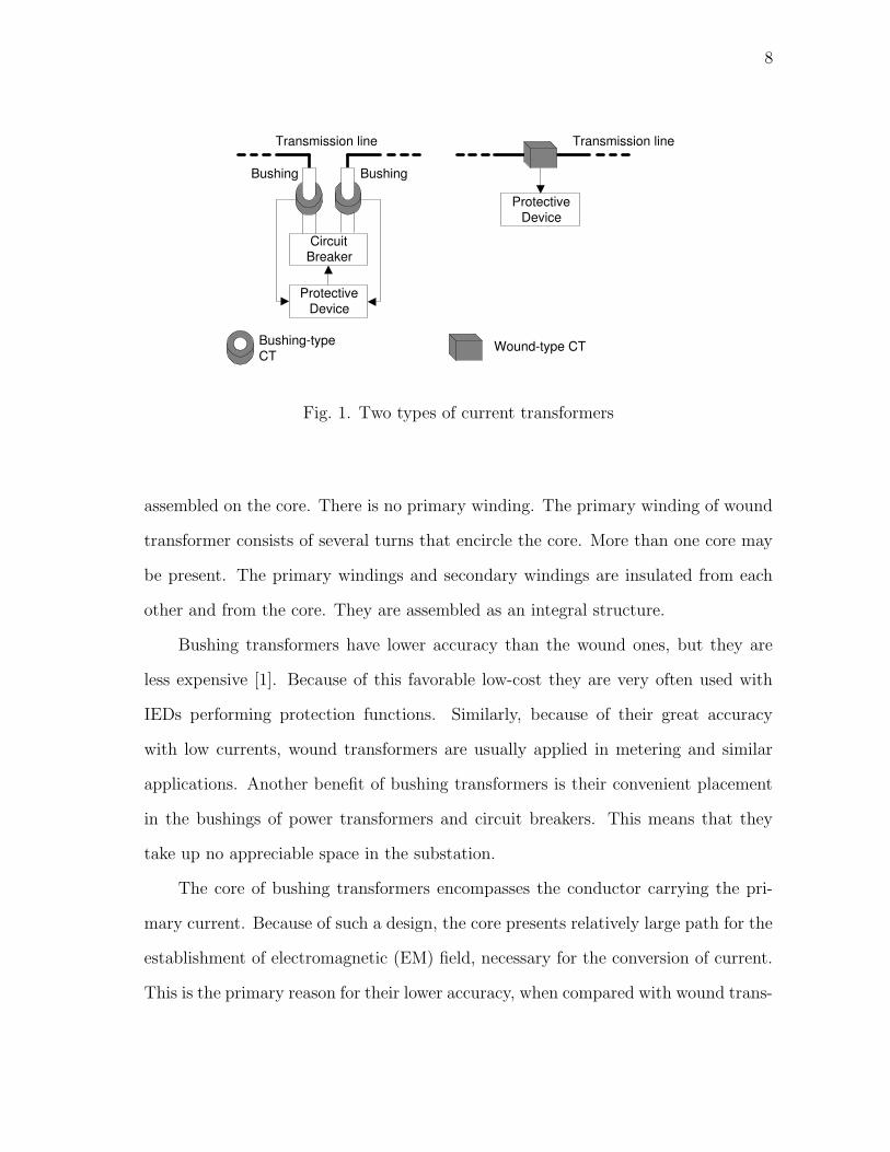
There are two types of current transformers (CT) available: bushing and wound [1],

[22], as shown in Fig. 1. The core of a bushing transformer is annular, while the

secondary winding is insulated from the core. The secondary winding is permanently

8

Protective Device

Circuit Breaker

Transmission line

Bushing Bushing

Protective Device

Transmission line

Wound-type CT Bushing-type CT

Fig. 1. Two types of current transformers

assembled on the core. There is no primary winding. The primary winding of wound

transformer consists of several turns that encircle the core. More than one core may

be present. The primary windings and secondary windings are insulated from each

other and from the core. They are assembled as an integral structure.

Bushing transformers have lower accuracy than the wound ones, but they are

less expensive [1]. Because of this favorable low-cost they are very often used with

IEDs performing protection functions. Similarly, because of their great accuracy

with low currents, wound transformers are usually applied in metering and similar

applications. Another benefit of bushing transformers is their convenient placement

in the bushings of power transformers and circuit breakers. This means that they

take up no appreciable space in the substation.

The core of bushing transformers encompasses the conductor carrying the pri-

mary current. Because of such a design, the core presents relatively large path for the

establishment of electromagnetic (EM) field, necessary for the conversion of current.

This is the primary reason for their lower accuracy, when compared with wound trans-

9

formers. However, bushing transformers are also built with increased cross-sectional

area of iron in the core. The advantage of this is higher accuracy in scaling of fault

currents that are of large multiples of nominal current, when compared to wound

transformers. High accuracy for high fault currents is desirable in protective relaying.

Therefore, the bushing transformers are a good choice for protective applications.

2. Voltage Transformers

Voltage transformers are available in two types [1]:

1. Electromagnetic voltage transformer (VT)

2. Coupling-capacitor voltage transformer (CCVT)

Voltage transformer is very similar to conventional power transformer. Main differ-

ence is that voltage transformer is connected to a small and constant load. CCVT

has two main designs: 1) the coupling-capacitor device, 2) bushing device. The first

design consists of a series of capacitors (arranged in a stack), where the secondary of

the transformer is taken from the last capacitor in series (called auxiliary capacitor).

The second design uses capacitance bushings to produce secondary voltage at the

output.

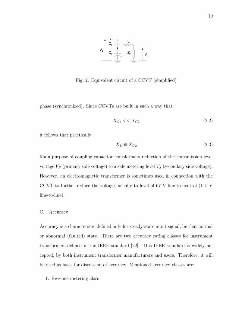
In order to better understand the operating principle of a CCVT, equivalent

circuit of a coupling-capacitor transformer is shown in Fig. 2 (ZB presents the trans-

former burden). The equivalent reactance of this circuit can be expressed as:

XL =XC1 · XC2

XC1 + XC2

(2.1)

By choosing values for XC1 and XC2, reactance XL can be adjusted. The purpose of

adjusting this reactance is to ensure that primary and the secondary voltages are in

10

Z B

L C 1

C 2 V S

V P

Fig. 2. Equivalent circuit of a CCVT (simplified)

phase (synchronized). Since CCVTs are built in such a way that:

XC1 << XC2 (2.2)

it follows that practically

XL∼= XC2 (2.3)

Main purpose of coupling-capacitor transformers reduction of the transmission-level

voltage VP (primary side voltage) to a safe metering level VS (secondary side voltage).

However, an electromagnetic transformer is sometimes used in connection with the

CCVT to further reduce the voltage, usually to level of 67 V line-to-neutral (115 V

line-to-line).

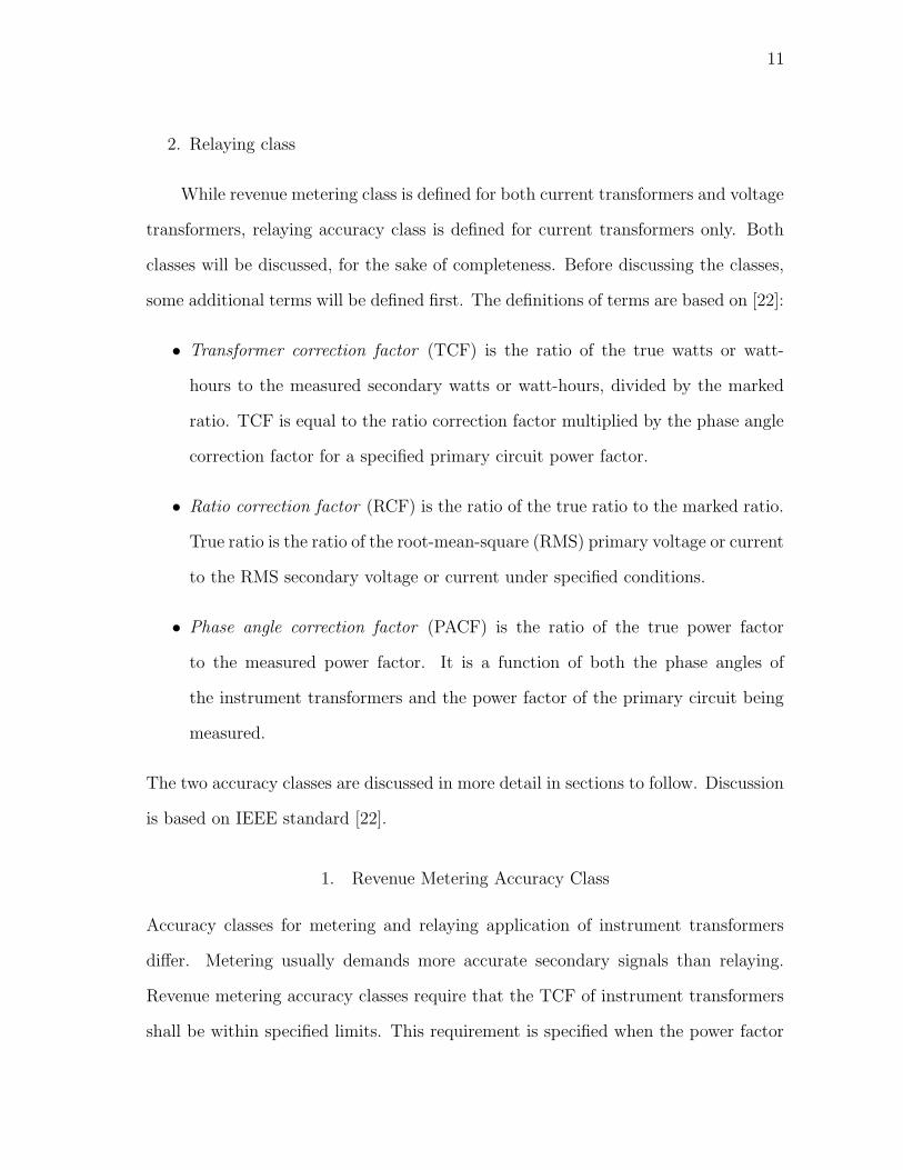
C. Accuracy

Accuracy is a characteristic defined only for steady-state input signal, be that normal

or abnormal (faulted) state. There are two accuracy rating classes for instrument

transformers defined in the IEEE standard [22]. This IEEE standard is widely ac-

cepted, by both instrument transformer manufacturers and users. Therefore, it will

be used as basis for discussion of accuracy. Mentioned accuracy classes are:

1. Revenue metering class

11

2. Relaying class

While revenue metering class is defined for both current transformers and voltage

transformers, relaying accuracy class is defined for current transformers only. Both

classes will be discussed, for the sake of completeness. Before discussing the classes,

some additional terms will be defined first. The definitions of terms are based on [22]:

• Transformer correction factor (TCF) is the ratio of the true watts or watt-

hours to the measured secondary watts or watt-hours, divided by the marked

ratio. TCF is equal to the ratio correction factor multiplied by the phase angle

correction factor for a specified primary circuit power factor.

• Ratio correction factor (RCF) is the ratio of the true ratio to the marked ratio.

True ratio is the ratio of the root-mean-square (RMS) primary voltage or current

to the RMS secondary voltage or current under specified conditions.

• Phase angle correction factor (PACF) is the ratio of the true power factor

to the measured power factor. It is a function of both the phase angles of

the instrument transformers and the power factor of the primary circuit being

measured.

The two accuracy classes are discussed in more detail in sections to follow. Discussion

is based on IEEE standard [22].

1. Revenue Metering Accuracy Class

Accuracy classes for metering and relaying application of instrument transformers

differ. Metering usually demands more accurate secondary signals than relaying.

Revenue metering accuracy classes require that the TCF of instrument transformers

shall be within specified limits. This requirement is specified when the power factor

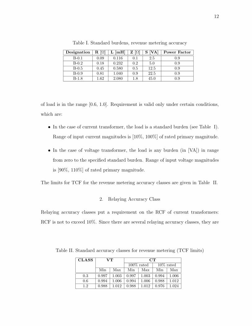
12

Table I. Standard burdens, revenue metering accuracy

Designation R [Ω] L [mH] Z [Ω] S [VA] Power Factor

B-0.1 0.09 0.116 0.1 2.5 0.9B-0.2 0.18 0.232 0.2 5.0 0.9B-0.5 0.45 0.580 0.5 12.5 0.9B-0.9 0.81 1.040 0.9 22.5 0.9B-1.8 1.62 2.080 1.8 45.0 0.9

of load is in the range [0.6, 1.0]. Requirement is valid only under certain conditions,

which are:

• In the case of current transformer, the load is a standard burden (see Table I).

Range of input current magnitudes is [10%, 100%] of rated primary magnitude.

• In the case of voltage transformer, the load is any burden (in [VA]) in range

from zero to the specified standard burden. Range of input voltage magnitudes

is [90%, 110%] of rated primary magnitude.

The limits for TCF for the revenue metering accuracy classes are given in Table II.

2. Relaying Accuracy Class

Relaying accuracy classes put a requirement on the RCF of current transformers:

RCF is not to exceed 10%. Since there are several relaying accuracy classes, they are

Table II. Standard accuracy classes for revenue metering (TCF limits)

CLASS VT CT100% rated 10% rated

Min Max Min Max Min Max

0.3 0.997 1.003 0.997 1.003 0.994 1.0060.6 0.994 1.006 0.994 1.006 0.988 1.0121.2 0.988 1.012 0.988 1.012 0.976 1.024

13

Table III. Standard burdens, relaying accuracy

Designation R [Ω] L [mH] Z [Ω] S [VA] Power Factor

B-1 0.50 2.300 1.0 25.0 0.5B-2 1.00 4.600 2.0 50.0 0.5B-4 2.00 9.200 4.0 100.0 0.5B-8 4.00 18.400 8.0 200.0 0.5

designated by a letter and a secondary terminal voltage rating, as follows:

1. Letter C, K, or T. Flux leakage in the core of current transformers, designated

as C and K, does not influence transformer ratio. Additional feature of current

transformer designated K is having a knee-point voltage at least 70% of the

rated secondary voltage magnitude. Current transformer designated as T have

appreciable flux leakage in the core. This leakage deteriorates transformer ratio

significantly.

2. Secondary terminal voltage rating. This voltage is a maximum voltage, pro-

duced by a standard burden and input current of magnitude 20 times the rated

one, that will still keep the transformer ratio from exceeding 10 % of RCF.

Standard burdens are given in Tables I and III. Rated secondary terminal voltages,

associated with standard burdens, are given in Table IV.

Table IV. Secondary terminal voltages and associated standard burdens

Voltage [V] 10 20 50 100 200 400 800Burden B-0.1 B-0.2 B-0.5 B-1 B-2 B-4 B-8

14

D. Frequency Response

Frequency response can be evaluated only for linear systems. In general, instrument

transformers are not linear devices. However, instrument transformers are usually

properly sized (with parameters of various components) to operate only in linear

region. This means that most of the time, instrument transformers can be regarded

as linear devices. Frequency response in such cases is discussed in following sections.


Magnitude of the frequency response of a typical current transformer is constant over

a very wide frequency range (up to 50 kHz) [7]. The phase angle is also constant

and has zero value. For practical purposes current transformer can be regarded as

having no impact on the spectral content of the input signal, under condition that

electromagnetic flux in the core is in the linear region. In case the flux goes out of

the linear region, transformers are no longer considered linear devices, which means

that frequency response cannot be evaluated. This situation is discussed in section E

of this chapter.


Similarly as in the case of current transformers, frequency response of voltage trans-

formers and CCVTs can be evaluated only when the magnetic flux in the core is in the

linear region. Cases of flux being in the non-linear region are discussed in Section E

of this chapter.

Typical frequency range of signals used by IEDs is up to 10 kHz. In this range,

voltage transformer frequency response acts as a low-pass filter. The cut-off frequency

depends on the parameters of voltage transformer. Most notable parameters (that

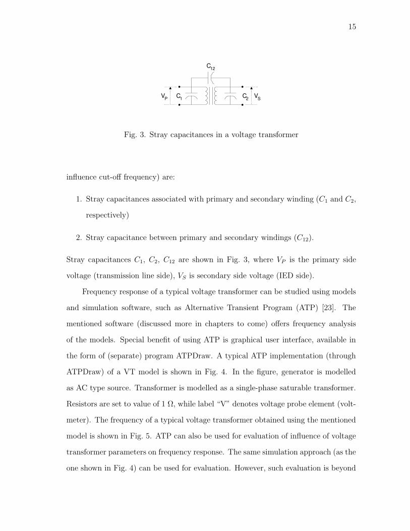
15

C 1

C 12

V S V P C 2

Fig. 3. Stray capacitances in a voltage transformer

influence cut-off frequency) are:

1. Stray capacitances associated with primary and secondary winding (C1 and C2,

respectively)

2. Stray capacitance between primary and secondary windings (C12).

Stray capacitances C1, C2, C12 are shown in Fig. 3, where VP is the primary side

voltage (transmission line side), VS is secondary side voltage (IED side).

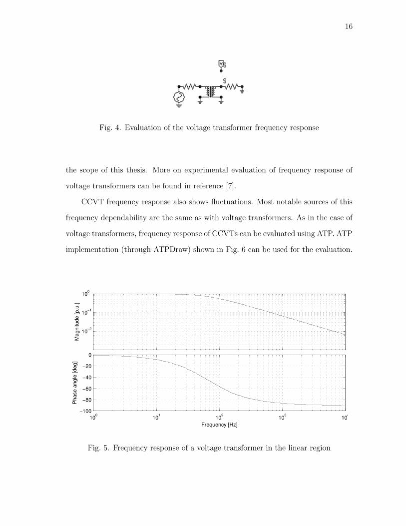
Frequency response of a typical voltage transformer can be studied using models

and simulation software, such as Alternative Transient Program (ATP) [23]. The

mentioned software (discussed more in chapters to come) offers frequency analysis

of the models. Special benefit of using ATP is graphical user interface, available in

the form of (separate) program ATPDraw. A typical ATP implementation (through

ATPDraw) of a VT model is shown in Fig. 4. In the figure, generator is modelled

as AC type source. Transformer is modelled as a single-phase saturable transformer.

Resistors are set to value of 1 Ω, while label “V” denotes voltage probe element (volt-

meter). The frequency of a typical voltage transformer obtained using the mentioned

model is shown in Fig. 5. ATP can also be used for evaluation of influence of voltage

transformer parameters on frequency response. The same simulation approach (as the

one shown in Fig. 4) can be used for evaluation. However, such evaluation is beyond

16

Fig. 4. Evaluation of the voltage transformer frequency response

the scope of this thesis. More on experimental evaluation of frequency response of

voltage transformers can be found in reference [7].

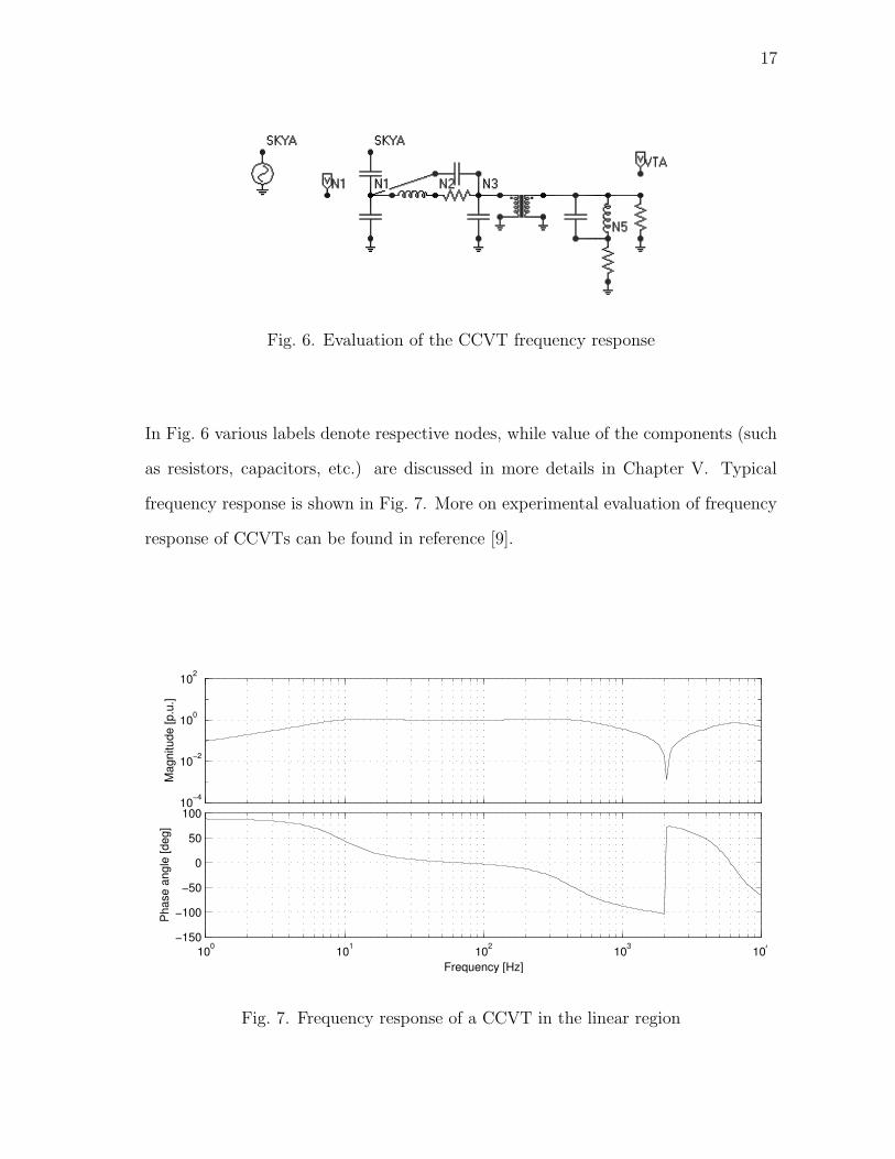
CCVT frequency response also shows fluctuations. Most notable sources of this

frequency dependability are the same as with voltage transformers. As in the case of

voltage transformers, frequency response of CCVTs can be evaluated using ATP. ATP

implementation (through ATPDraw) shown in Fig. 6 can be used for the evaluation.

10−2

10−1

100

Frequency [Hz]

Mag

nitu

de [p

.u.]

100 101 102 103 104−100

−80

−60

−40

−20

0

Frequency [Hz]

Pha

se a

ngle

[deg

]

Fig. 5. Frequency response of a voltage transformer in the linear region

17

Fig. 6. Evaluation of the CCVT frequency response

In Fig. 6 various labels denote respective nodes, while value of the components (such

as resistors, capacitors, etc.) are discussed in more details in Chapter V. Typical

frequency response is shown in Fig. 7. More on experimental evaluation of frequency

response of CCVTs can be found in reference [9].

10−4

10−2

100

102

Mag

nitu

de [p

.u.]

Frequency [Hz]

100 101 102 103 104−150

−100

−50

0

50

100

Frequency [Hz]

Pha

se a

ngle

[deg

]

Fig. 7. Frequency response of a CCVT in the linear region

18

E. Transient Response


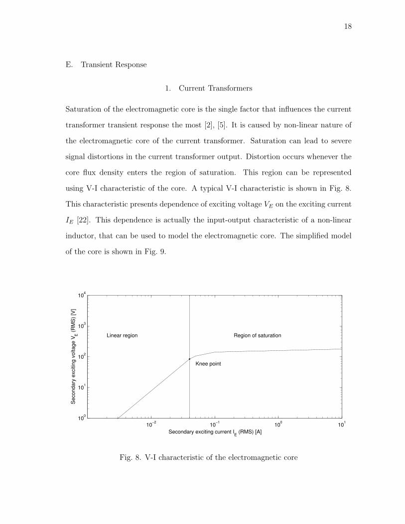
Saturation of the electromagnetic core is the single factor that influences the current

transformer transient response the most [2], [5]. It is caused by non-linear nature of

the electromagnetic core of the current transformer. Saturation can lead to severe

signal distortions in the current transformer output. Distortion occurs whenever the

core flux density enters the region of saturation. This region can be represented

using V-I characteristic of the core. A typical V-I characteristic is shown in Fig. 8.

This characteristic presents dependence of exciting voltage VE on the exciting current

IE [22]. This dependence is actually the input-output characteristic of a non-linear

inductor, that can be used to model the electromagnetic core. The simplified model

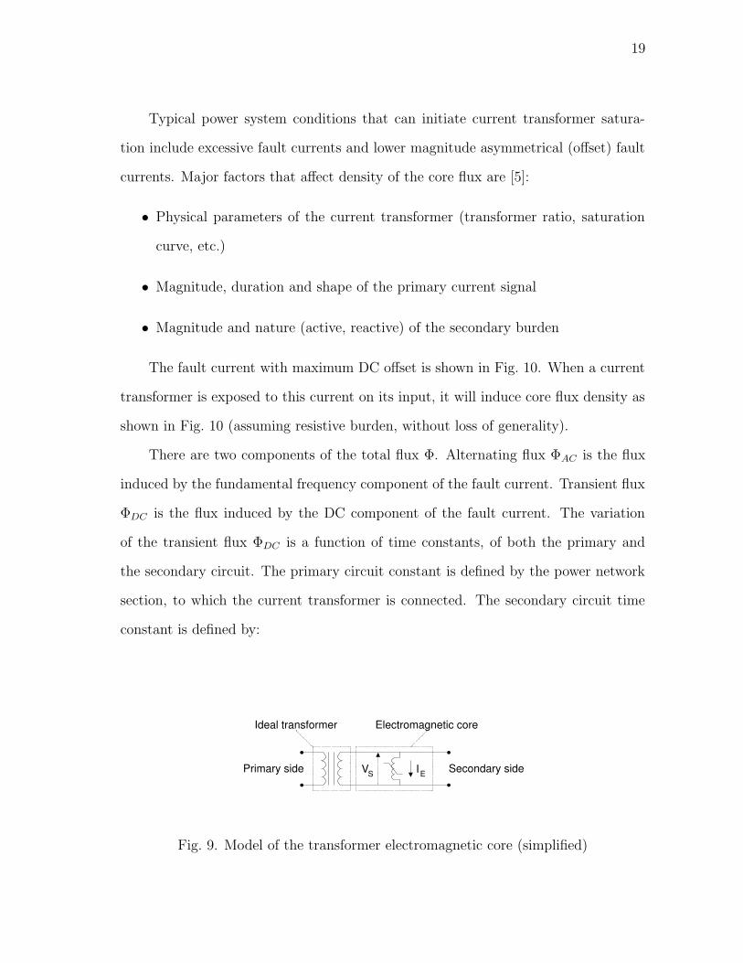
of the core is shown in Fig. 9.

10−2 10−1 100 101100

101

102

103

104

Secondary exciting current IE (RMS) [A]

Sec

onda

ry e

xciti

ng v

olta

ge V

E (R

MS

) [V

]

Linear region Region of saturation

Knee point

Fig. 8. V-I characteristic of the electromagnetic core

19

Typical power system conditions that can initiate current transformer satura-

tion include excessive fault currents and lower magnitude asymmetrical (offset) fault

currents. Major factors that affect density of the core flux are [5]:

• Physical parameters of the current transformer (transformer ratio, saturation

curve, etc.)

• Magnitude, duration and shape of the primary current signal

• Magnitude and nature (active, reactive) of the secondary burden

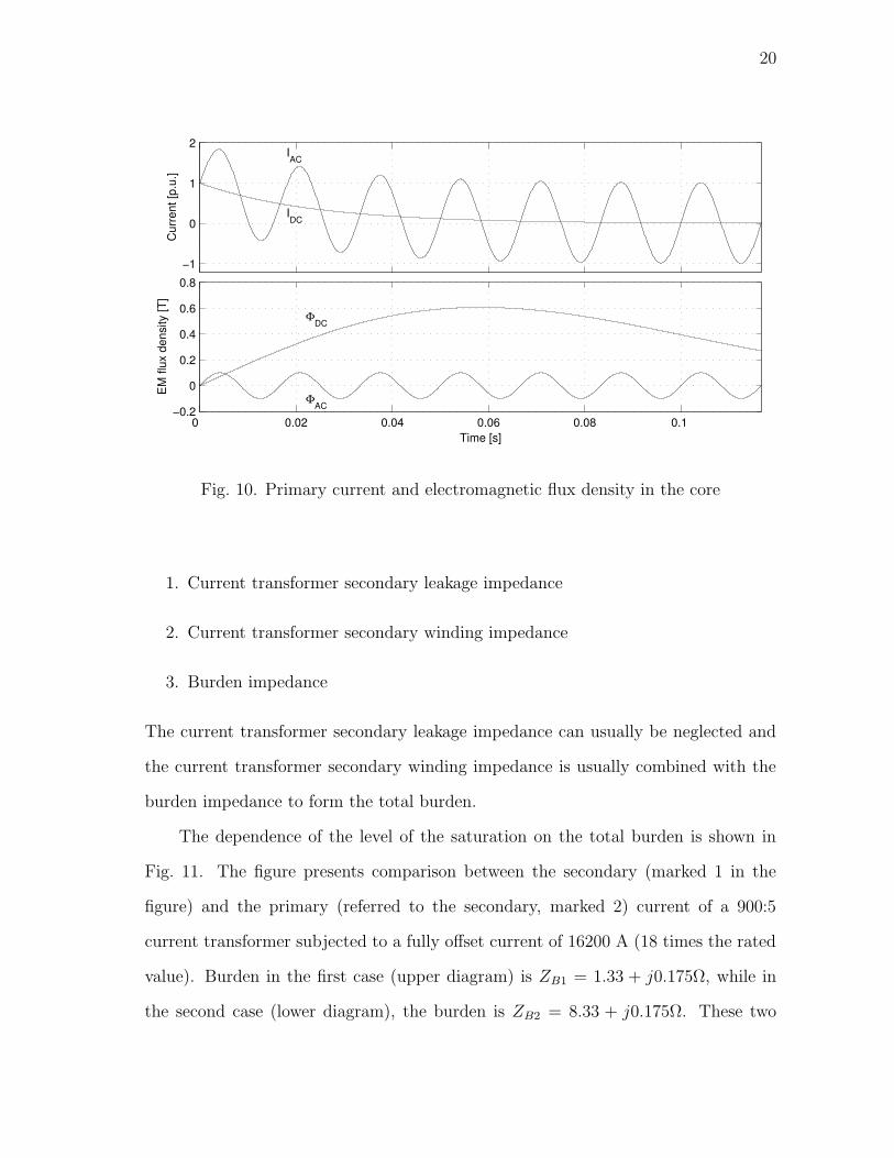
The fault current with maximum DC offset is shown in Fig. 10. When a current

transformer is exposed to this current on its input, it will induce core flux density as

shown in Fig. 10 (assuming resistive burden, without loss of generality).

There are two components of the total flux Φ. Alternating flux ΦAC is the flux

induced by the fundamental frequency component of the fault current. Transient flux

ΦDC is the flux induced by the DC component of the fault current. The variation

of the transient flux ΦDC is a function of time constants, of both the primary and

the secondary circuit. The primary circuit constant is defined by the power network

section, to which the current transformer is connected. The secondary circuit time

constant is defined by:

Ideal transformer Electromagnetic core

Primary side Secondary side V S I E

Fig. 9. Model of the transformer electromagnetic core (simplified)

20

−1

0

1

2

Cur

rent

[p.u

.]

Time [s]

IAC

IDC

0 0.02 0.04 0.06 0.08 0.1 −0.2

0

0.2

0.4

0.6

0.8

EM

flux

den

sity

[T]

Time [s]

ΦAC

ΦDC

Fig. 10. Primary current and electromagnetic flux density in the core

1. Current transformer secondary leakage impedance

2. Current transformer secondary winding impedance

3. Burden impedance

The current transformer secondary leakage impedance can usually be neglected and

the current transformer secondary winding impedance is usually combined with the

burden impedance to form the total burden.

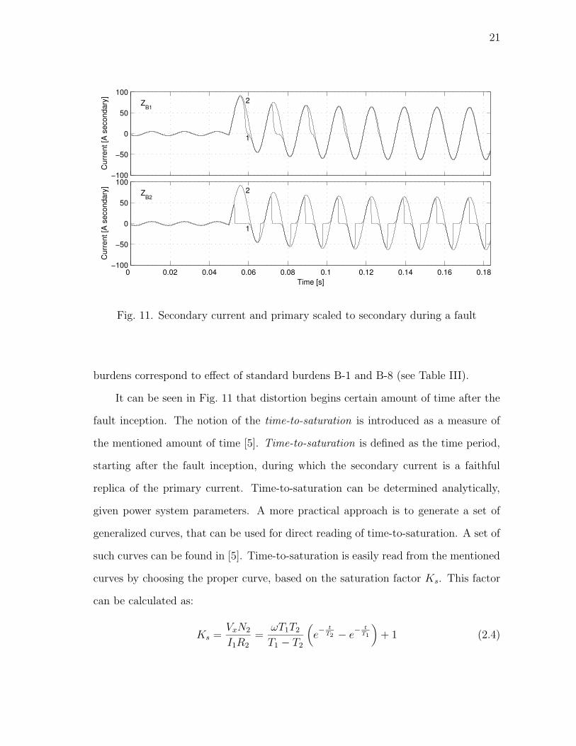
The dependence of the level of the saturation on the total burden is shown in

Fig. 11. The figure presents comparison between the secondary (marked 1 in the

figure) and the primary (referred to the secondary, marked 2) current of a 900:5

current transformer subjected to a fully offset current of 16200 A (18 times the rated

value). Burden in the first case (upper diagram) is ZB1 = 1.33 + j0.175Ω, while in

the second case (lower diagram), the burden is ZB2 = 8.33 + j0.175Ω. These two

21

−100

−50

0

50

100

Time [s]

Cur

rent

[A s

econ

dary

]Z

B12

1

0 0.02 0.04 0.06 0.08 0.1 0.12 0.14 0.16 0.18−100

−50

0

50

100

Time [s]

Cur

rent

[A s

econ

dary

]

ZB2

2

1

Fig. 11. Secondary current and primary scaled to secondary during a fault

burdens correspond to effect of standard burdens B-1 and B-8 (see Table III).

It can be seen in Fig. 11 that distortion begins certain amount of time after the

fault inception. The notion of the time-to-saturation is introduced as a measure of

the mentioned amount of time [5]. Time-to-saturation is defined as the time period,

starting after the fault inception, during which the secondary current is a faithful

replica of the primary current. Time-to-saturation can be determined analytically,

given power system parameters. A more practical approach is to generate a set of

generalized curves, that can be used for direct reading of time-to-saturation. A set of

such curves can be found in [5]. Time-to-saturation is easily read from the mentioned

curves by choosing the proper curve, based on the saturation factor Ks. This factor

can be calculated as:

Ks =VxN2

I1R2

=ωT1T2

T1 − T2

(

e− t

T2 − e− t

T1

)

+ 1 (2.4)

22

where Vx is RMS saturation voltage, N2 is the number of the secondary windings,

I1 is the primary current magnitude, R2 is the resistance of total secondary burden

(winding plus external resistance), ω is 2π · 60 rad.


There are two power system conditions that can cause problematic response of voltage

transformers. The conditions are [9]:

1. Sudden decrease of voltage at the transformer terminals (due to e.g. a fault

close to voltage transformer)

2. Sudden overvoltages (on the sound phases due to e.g. line-to-ground faults

elsewhere in the power network)

First type of condition can produce internal oscillations within the electromag-

netic core of electromagnetic voltage transformers. They appear on the secondary

winding output in the form of high-frequency oscillations (frequency much higher

than the system frequency, sometimes called ringing). The damping time of such

oscillations is usually between 15 and 20 ms. In case of CCVTs, oscillations at the

secondary winding, caused by the energy stored in the capacitive and inductive ele-

ments of the device, can last up to 100 ms. Second type of power system condition

can lead to saturation of the electromagnetic core. The mechanism and effect of the

saturation of the core is the same as with current transformers (which was already

discussed).

The mentioned oscillations are commonly referred to as the subsidence transient.

The subsidence transient generated by CCVTs is studied in reference [6]. In the study,

subsidence transient is defined as an error voltage appearing at the output terminals

of a coupling-capacitor voltage transformer resulting from a sudden and significant

23

−100

−50

0

50

100

Time [s]

Vol

tage

[V s

econ

dary

]Z

B1

1

0 0.02 0.04 0.06 0.08 0.1 0.12 0.14 0.16

−100

−50

0

50

100

Vol

tage

[V s

econ

dary

]

Time [s]

ZB2 22

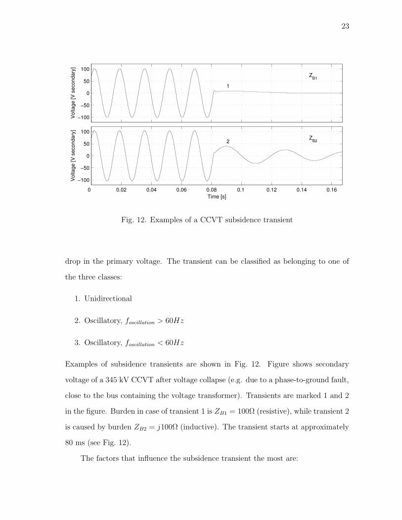
Fig. 12. Examples of a CCVT subsidence transient

drop in the primary voltage. The transient can be classified as belonging to one of

the three classes:

1. Unidirectional

2. Oscillatory, foscillation > 60Hz

3. Oscillatory, foscillation < 60Hz

Examples of subsidence transients are shown in Fig. 12. Figure shows secondary

voltage of a 345 kV CCVT after voltage collapse (e.g. due to a phase-to-ground fault,

close to the bus containing the voltage transformer). Transients are marked 1 and 2

in the figure. Burden in case of transient 1 is ZB1 = 100Ω (resistive), while transient 2

is caused by burden ZB2 = j100Ω (inductive). The transient starts at approximately

80 ms (see Fig. 12).

The factors that influence the subsidence transient the most are:

24

1. Coupling-capacitor voltage transformer burden

2. Coupling-capacitor voltage transformer design

3. Ferroresonance suppression circuit (FSC)

The influence of FSC on transient response of voltage transformers will be explained

in the text to follow. Experimental evaluation shows that elements of the coupling-

capacitor voltage transformer burden, that influence the subsidence transient, are

[6]:

1. Burden magnitude. The influence of the burden is lessened when the magnitude

of the used burden is smaller than the nominal one.

2. Burden power factor. Decrease in the power factor leads to lessening of the

subsidence transient.

3. Composition and connection of the burden. If there are inductive elements

present in the CCVT that have a high Q factor, the subsidence transient be-

comes great. However, the subsidence can be lessened by using series RL burden.

The subsidence transient is affected by surge capacitors in a minor way.

Coupling-capacitor voltage transformers may also contain a ferroresonance sup-

pression circuit (FSC) connected on the secondary side [24]. Due to their design,

FSC may impact CCVT transient response in certain cases. FSC designs, accord-

ing to their status during the transformer operation, can be divided into two main

operational modes:

• Active mode. This mode is achieved by connecting capacitors and iron core

inductors in parallel, at the secondary. The mentioned elements are tuned to

25

the fundamental frequency. Usually, such a construction is permanently placed

on the secondary side.

• Passive mode. This mode of operation is achieved by connecting only a resistor

at the secondary. Optionally, a gap or an electronic circuit can be placed in

series with the resistor. These elements are activated whenever an over voltage

occurs. Such a configuration has no effect on the voltage transformer transient

response in case there is no overvoltage.

F. Conclusion

This chapter reviewed typical instrument transformer designs, their characteristics

and their impacts on signals distortions. Typical current transformer designs - bush-

ing and wound, as well as typical VT/CCVT designs were described from the stand-

point of protection system. Advantages and disadvantages of some designs over other

designs were addressed.

Three most notable instrument transformer characteristics - accuracy, frequency

response and transient response, were investigated. It was shown that all three charac-

teristics can lead to distortions. Main source of distortions with current transformers

is the saturation. Main source of distortions with VTs/CCVTs is the subsidence

transient and ferroresonance. Causes and mechanisms of mentioned distortions were

discussed. Means of lessening their impact were also addressed.

The conclusion is that impact of instrument transformer designs and charac-

teristics on distortions may be significant. When the power system conditions are

adequate, output signal can be significantly different from the scaled-down version

of input signal. This presents motivation to investigate influence of distortions on

protective devices. This issue is addressed in the next chapter.

26

CHAPTER III

PROTECTION SYSTEM SENSITIVITY TO SIGNAL DISTORTIONS

A. Introduction

Algorithms inside protective devices are designed to achieve maximum selectivity and

minimum operational time for fault waveforms as inputs. Algorithm performance in

case of artificial deviations from such input signals is hard to predict. Depending on

type and extent of deviation, protective devices might be “fooled” into making wrong

decisions, such as unnecessarily isolating network sections, or failing to disconnect

faulted component.

This chapter analyzes sensitivity of protection system to artificial distortions in

current and voltage signals on input. Core of protection system are IEDs - Intelligent

Electronic Devices. Their elements and functions are described first. Next, the men-

tioned sensitivity is established using a simple test method. Finally, negative impacts

of distortions are investigated. Material in this chapter demonstrates the necessity

for evaluation of influence of signal distortions.

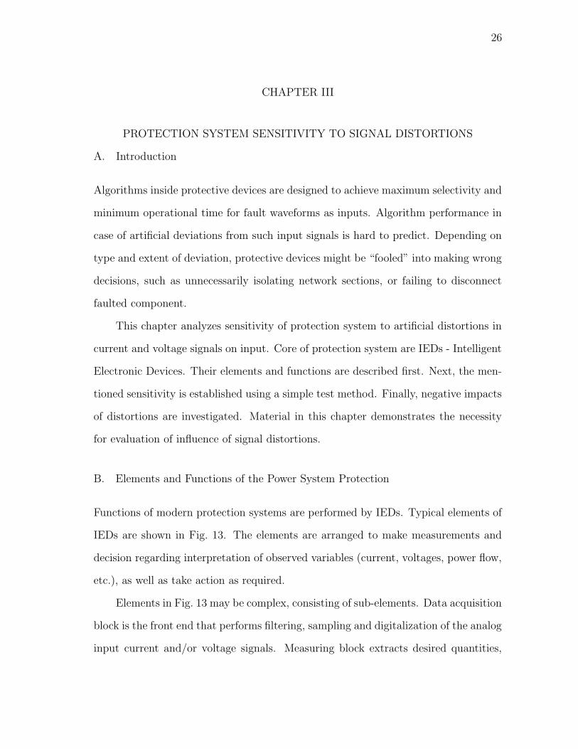
B. Elements and Functions of the Power System Protection

Functions of modern protection systems are performed by IEDs. Typical elements of

IEDs are shown in Fig. 13. The elements are arranged to make measurements and

decision regarding interpretation of observed variables (current, voltages, power flow,

etc.), as well as take action as required.

Elements in Fig. 13 may be complex, consisting of sub-elements. Data acquisition

block is the front end that performs filtering, sampling and digitalization of the analog

input current and/or voltage signals. Measuring block extracts desired quantities,

27

Data Acquisition

Measure- ment

Decision Making

Voltage signals

Current signals

Trip Alarm Control Data

Fig. 13. Functional elements of a typical IED

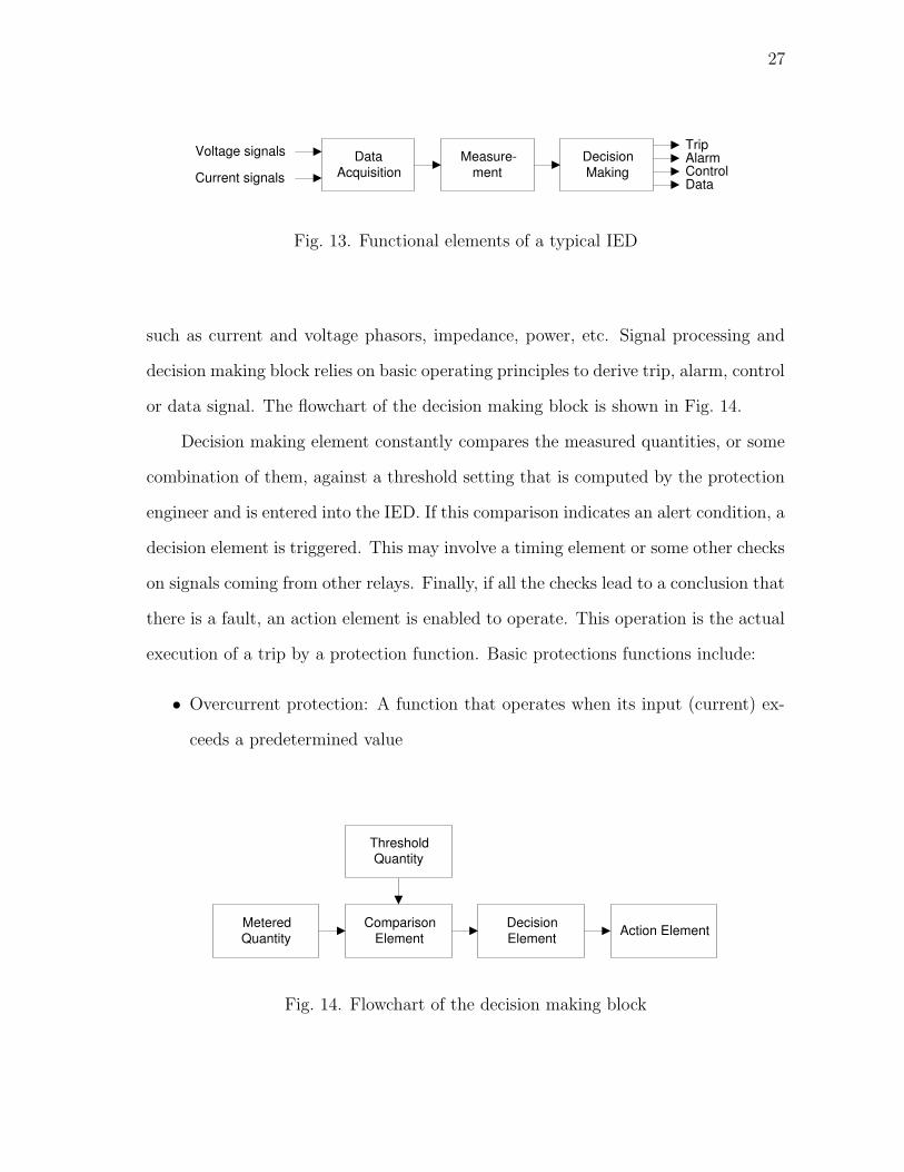
such as current and voltage phasors, impedance, power, etc. Signal processing and

decision making block relies on basic operating principles to derive trip, alarm, control

or data signal. The flowchart of the decision making block is shown in Fig. 14.

Decision making element constantly compares the measured quantities, or some

combination of them, against a threshold setting that is computed by the protection

engineer and is entered into the IED. If this comparison indicates an alert condition, a

decision element is triggered. This may involve a timing element or some other checks

on signals coming from other relays. Finally, if all the checks lead to a conclusion that

there is a fault, an action element is enabled to operate. This operation is the actual

execution of a trip by a protection function. Basic protections functions include:

• Overcurrent protection: A function that operates when its input (current) ex-

ceeds a predetermined value

Metered Quantity

Comparison Element

Decision Element Action Element

Threshold Quantity

Fig. 14. Flowchart of the decision making block

28

• Directional protection: A function that picks up for faults in one direction, and

is restrained for faults in the other direction

• Differential protection: A function that is intended to respond to a difference be-

tween incoming and outgoing electrical quantities associated with the protected

apparatus

• Distance protection: A function used for protection of transmission lines whose

response to the input quantities is primarily a function of the electrical distance

between the relay location and the fault point

• Pilot protection: A function that is a form of the transmission line protection

that uses a communication channel as the means of comparing relay actions at

the line terminals

C. Types of Signal Distortions

Possible conditions of a power system can be divided in two general categories:

1. Normal condition

2. Abnormal (faulted) condition

Power systems often carry signals that are corrupted in one way of another,

irrespective of the condition. Dominant distortions in normal condition are power

quality (PQ) disturbances. There are several different definitions of PQ disturbances

in the literature [25].

Distortions that are dominant in abnormal (faulted) condition are transients.

Transient are phenomena caused by power system’s inability to instantaneously trans-

fer energy, due to presence of energy-storing components, such as inductor and ca-

pacitor banks.

29

This thesis will address protection system sensitivity only to signals belonging

to the second category, abnormal (faulted) condition.

Field application has shown that instrument transformers do not cause signifi-

cant signal distortions during normal power condition, while they may induce severe

distortions during abnormal conditions (see Chapter II). General explanation for such

a performance is as follows:

• Instrument transformers are designed with normal conditions in mind. This

means that components of the design (such as electromagnetic core, various ca-

pacitors, inductors, etc.) are chosen to operate in linear regions, when exposed

to signals up to certain magnitudes (component ratings). Disturbances in nor-

mal operation do not cause these elements to leave linear region of operation

[5], [6], [8], [9]. In order to properly size (select) mentioned transformer com-

ponents, study has to be performed, to calculate maximum operating current

under all expected disturbances, such as harmonic components, power quality

events, and similar.

• During abnormal (faulted) conditions, current and voltage magnitudes can

change rapidly (within fractions of a 60 Hz cycle), in the range of thousands of

volts and amperes. If the change of signal magnitudes is sufficient (in current

power systems it often is), instrument transformers will be moved out of linear

region of operation.

D. Protection Function Sensitivity to Signal Distortions

A simple method can be used to establish IED sensitivity to input signal distortions.

The method proposed here covers typical distortions caused by instrument transform-

ers (see Chapter II). However, any kind of distortion can be evaluated for impact on

30

IEDs.

The method can be summarized as follows: IED sensitivity can be checked by

comparing IED response (output) when exposed to different levels of distortions in

the same input signal. This approach can be found in literature [26], [27].

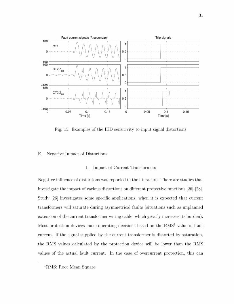
The method can be illustrated by sensitivity of overcurrent protection IED to

current transformer saturation. A simple simulation was carried out on models of

current transformers and IEDs. Results are shown in Fig. 15. In order to gener-

ate signals with different levels of saturation, two current transformer models were

used for scaling-down of primary side signals. Difference between models is the V-I

characteristic of the electromagnetic core. The two characteristics are discussed in

Chapter V. IED input signals produced by the two current transformers (shown in

Fig. 15) show different levels of distortion. Output signals of IED models show the

same response for both input signals. However, when burden of the second current

transformer was increased from ZB1 = 1.33 + j0.175Ω to ZB2 = 8.33 + j0.175Ω, IED

model showed significantly different response, also shown in Fig. 15. Conclusion is

that IED model is sensitive to distortion levels above a certain threshold. Questions

that arise from the conclusion are:

1. Are there negative impacts of distortions on IED performance, or can they be

neglected ? (i.e. is IED sensitivity significant enough to cause undesirably low

performance)

2. If there is negative impact, how can it be measured ?

The first question is discussed in the following section. The second question is dealt

with in the next chapter.

31

−100

0

100Fault current signals [A secondary]

CT1

−100

0

100CT2,Z

B1

0 0.05 0.1 0.15−100

0

100

Time [s]

CT2,ZB2

0

0.5

1

Trip signals

0

0.5

1

0 0.05 0.1 0.15

0

0.5

1

Time [s]

Fig. 15. Examples of the IED sensitivity to input signal distortions

E. Negative Impact of Distortions

1. Impact of Current Transformers

Negative influence of distortions was reported in the literature. There are studies that

investigate the impact of various distortions on different protective functions [26]-[28].

Study [26] investigates some specific applications, when it is expected that current

transformers will saturate during asymmetrical faults (situations such as unplanned

extension of the current transformer wiring cable, which greatly increases its burden).

Most protection devices make operating decisions based on the RMS1 value of fault

current. If the signal supplied by the current transformer is distorted by saturation,

the RMS values calculated by the protection device will be lower than the RMS

values of the actual fault current. In the case of overcurrent protection, this can

1RMS: Root Mean Square

32

cause protection device to trip with undesired delay.

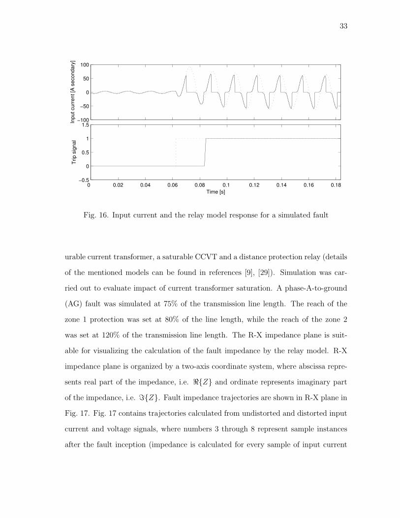
In order to verify these results, simulation was performed using models of a sat-

urable current transformer and an overcurrent protection relay (details of the men-

tioned models can be found in references [9], [29]). Simulation was carried out to

evaluate impact of current transformer saturation. A phase-A-to-ground (AG) fault

was simulated at 10% of the transmission line length at 0.05 s. The phase A fault

current (including a portion of the pre-fault steady state) is shown in Fig. 16. The

dotted line represents the primary current scaled to secondary, while the full line

represents the secondary current, which is supplied to the relay model. Fig. 16 also

shows the trip signal derived by the relay model (dotted line presents trip signal for

the undistorted input signal, while the full line presents trip signal for input distorted

by saturation). Fig. 16 shows delayed tripping (more than one 60 Hz cycle). The

delay is long enough that it may present threat to safe operation of the entire power

system.

Work presented in reference [30] addresses impact of current transformers on the

distance protection. The results show that when the current transformer undergoes

distortion, the measuring algorithm detects the fundamental frequency component of

the fault current with a lower value than the actual. This kind of distortion can make

the calculated impedance trajectory to enter and exit the zone of protection before

the trip signal is asserted, or the calculated trajectory may not enter the zone of

protection during the first cycle in which the fault occurred. Therefore, the effect of

the current transformer saturation can cause a delay in issuing a trip signal. It should

be noted that if the current transformer undergoes saturation by the symmetrical fault

current (i.e. when the exponential decay component is zero) the impedance trajectory

calculated by the measuring algorithm may never enter the zone of protection.

To verify the results from [30] simulation was performed using models of a sat-

33

−100

−50

0

50

100In

put c

urre

nt [A

sec

onda

ry]

0 0.02 0.04 0.06 0.08 0.1 0.12 0.14 0.16 0.18−0.5

0

0.5

1

1.5

Trip

sig

nal

Time [s]

Fig. 16. Input current and the relay model response for a simulated fault

urable current transformer, a saturable CCVT and a distance protection relay (details

of the mentioned models can be found in references [9], [29]). Simulation was car-

ried out to evaluate impact of current transformer saturation. A phase-A-to-ground

(AG) fault was simulated at 75% of the transmission line length. The reach of the

zone 1 protection was set at 80% of the line length, while the reach of the zone 2

was set at 120% of the transmission line length. The R-X impedance plane is suit-

able for visualizing the calculation of the fault impedance by the relay model. R-X

impedance plane is organized by a two-axis coordinate system, where abscissa repre-

sents real part of the impedance, i.e. <Z and ordinate represents imaginary part

of the impedance, i.e. =Z. Fault impedance trajectories are shown in R-X plane in

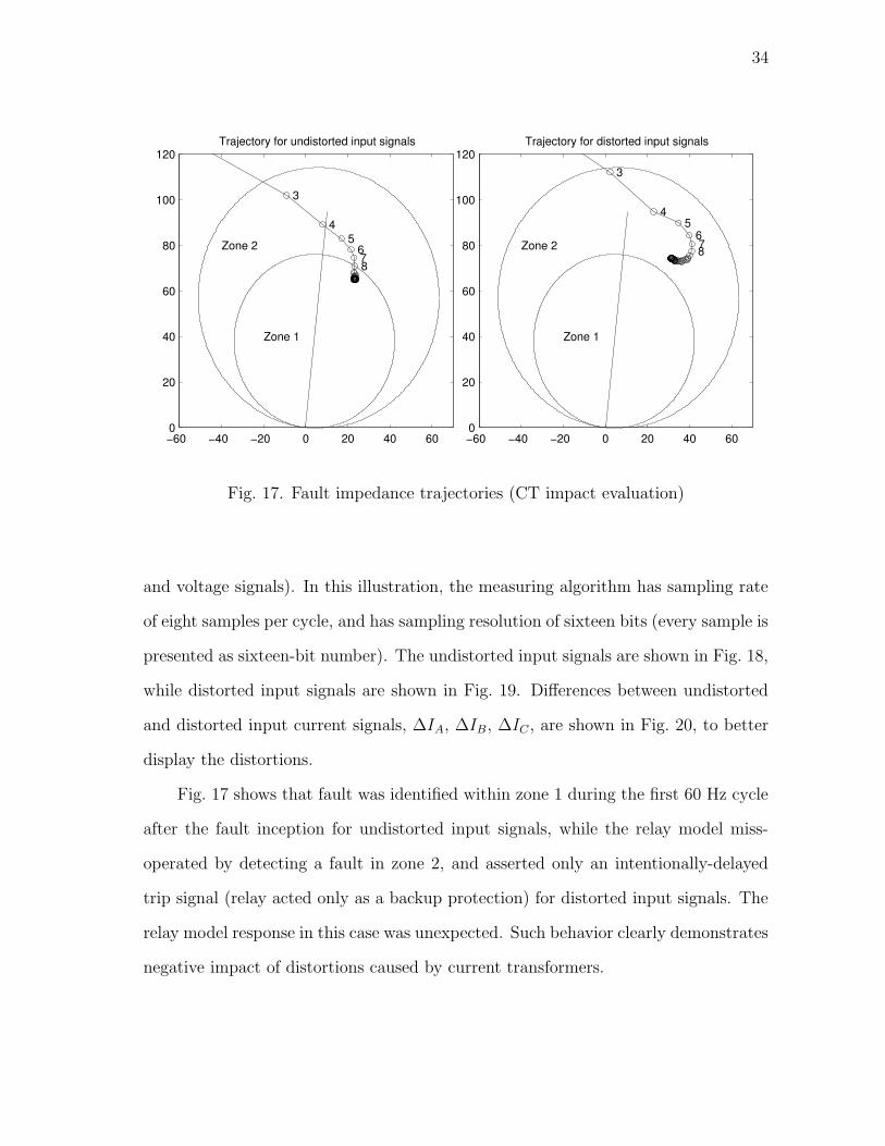
Fig. 17. Fig. 17 contains trajectories calculated from undistorted and distorted input

current and voltage signals, where numbers 3 through 8 represent sample instances

after the fault inception (impedance is calculated for every sample of input current

34

−60 −40 −20 0 20 40 600

20

40

60

80

100

120

3

45

678

Zone 1

Zone 2

Trajectory for undistorted input signals

−60 −40 −20 0 20 40 600

20

40

60

80

100

1203

45

678

Zone 1

Zone 2

Trajectory for distorted input signals

Fig. 17. Fault impedance trajectories (CT impact evaluation)

and voltage signals). In this illustration, the measuring algorithm has sampling rate

of eight samples per cycle, and has sampling resolution of sixteen bits (every sample is

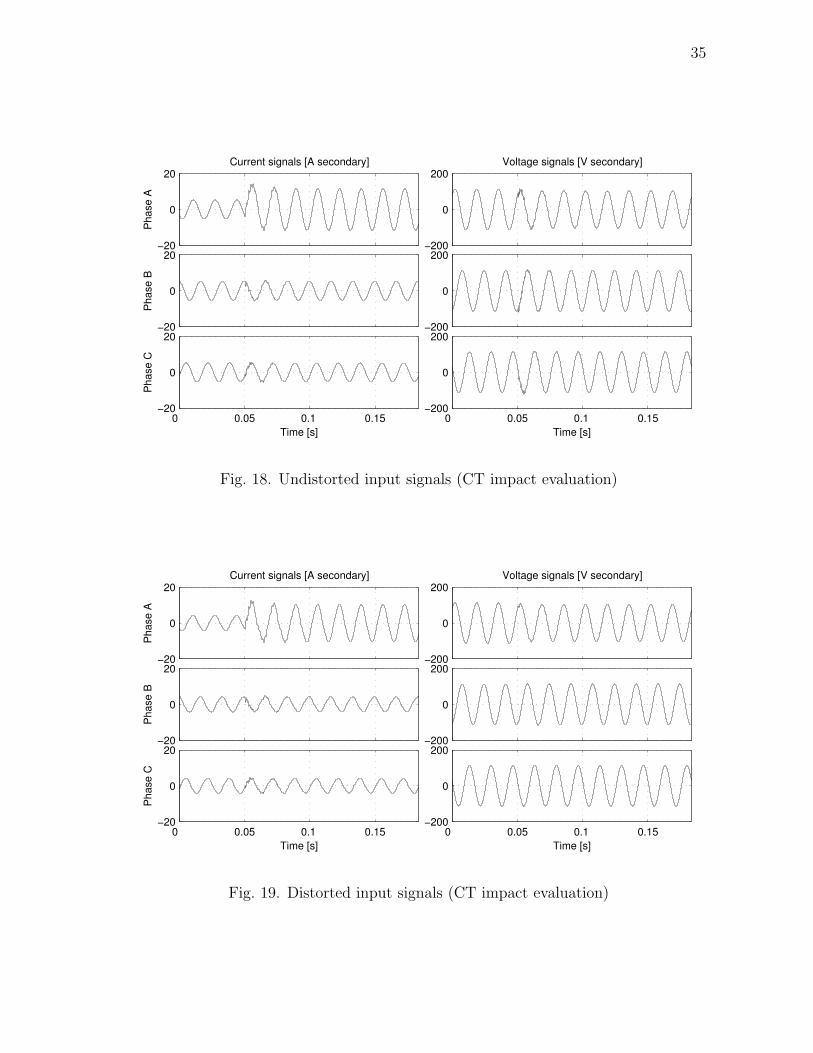
presented as sixteen-bit number). The undistorted input signals are shown in Fig. 18,

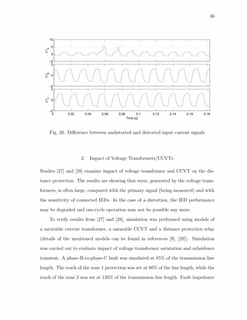
while distorted input signals are shown in Fig. 19. Differences between undistorted

and distorted input current signals, ∆IA, ∆IB, ∆IC , are shown in Fig. 20, to better

display the distortions.

Fig. 17 shows that fault was identified within zone 1 during the first 60 Hz cycle

after the fault inception for undistorted input signals, while the relay model miss-

operated by detecting a fault in zone 2, and asserted only an intentionally-delayed

trip signal (relay acted only as a backup protection) for distorted input signals. The

relay model response in this case was unexpected. Such behavior clearly demonstrates

negative impact of distortions caused by current transformers.

35

−20

0

20

Pha

se A

Current signals [A secondary]

−20

0

20

Pha

se B

0 0.05 0.1 0.15−20

0

20

Pha

se C

Time [s]

−200

0

200Voltage signals [V secondary]

−200

0

200

0 0.05 0.1 0.15−200

0

200

Time [s]

Fig. 18. Undistorted input signals (CT impact evaluation)

−20

0

20

Pha

se A


−20

0

20

Pha

se B

0 0.05 0.1 0.15−20

0

20

Pha

se C

Time [s]

−200

0


−200

0

200

0 0.05 0.1 0.15−200

0

200

Time [s]

Fig. 19. Distorted input signals (CT impact evaluation)

36

−5

0

5

10

∆ I A

−2

0

2

∆ I B

0 0.02 0.04 0.06 0.08 0.1 0.12 0.14 0.16 0.18−2

0

2

∆ I C

Time [s]

Fig. 20. Difference between undistorted and distorted input current signals

2. Impact of Voltage Transformers/CCVTs

Studies [27] and [28] examine impact of voltage transformer and CCVT on the dis-

tance protection. The results are showing that error, generated by the voltage trans-

formers, is often large, compared with the primary signal (being measured) and with

the sensitivity of connected IEDs. In the case of a distortion, the IED performance

may be degraded and one-cycle operation may not be possible any more.

To verify results from [27] and [28], simulation was performed using models of

a saturable current transformer, a saturable CCVT and a distance protection relay

(details of the mentioned models can be found in references [9], [29]). Simulation

was carried out to evaluate impact of voltage transformer saturation and subsidence

transient. A phase-B-to-phase-C fault was simulated at 85% of the transmission line

length. The reach of the zone 1 protection was set at 80% of the line length, while the

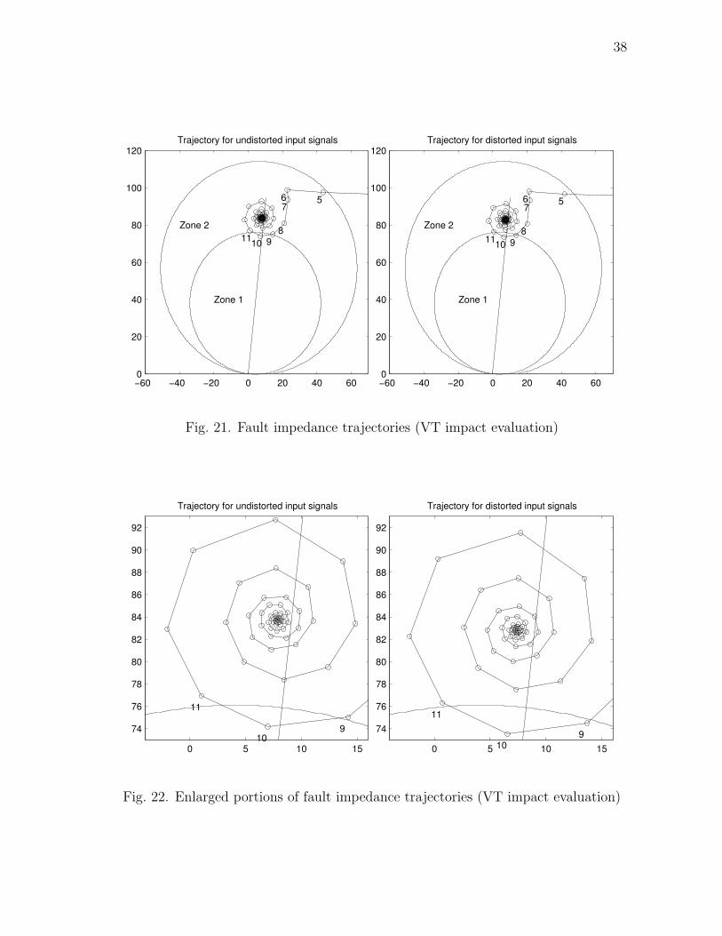
reach of the zone 2 was set at 120% of the transmission line length. Fault impedance

37

trajectories are shown in Fig. 21. Fig. 21 contains trajectories calculated from undis-

torted and distorted input current and voltage signals, where numbers 5 through 11

represent sample instances after the fault inception (impedance is calculated for ev-

ery sample of input current and voltage signals). In this illustration, the measuring

algorithm has sampling rate of eight samples per cycles, and has sampling resolution

of sixteen bits (every sample is presented as sixteen-bit number).

As can be seen, the trajectory indicates fault impedance within zone 2 for in-

stances 5,6,7,8. Fault impedance for instances 9,10,11 is in a critical vicinity of the

border line between zones 1 and 2. This critical vicinity is showed in more detail in

Fig. 22. Fig. 22 shows that fault impedance enters zone 1 only during one instance for

undistorted input signals, while the fault impedance remains in zone 1 during two in-

stances for distorted input signals. This additional instance of fault impedance being

in zone 1 is caused by CCVT-induced distortion. The relay model correctly operated

when supplied with undistorted input signals (relay model intentionally delayed trip

assertion). The relay model miss-operated when supplied with distorted input sig-

nals (relay model immediately asserted trip, as if the fault impedance was in zone

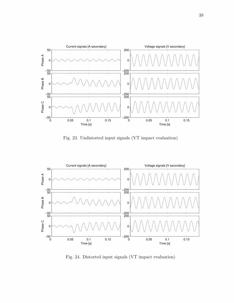
1). Undistorted input signals are shown in Fig. 23, while distorted input signals are

shown in Fig. 24. Since it is virtually impossible to identify the difference between the

Figs. 23 and 24, differences between undistorted and distorted input voltage signals

∆VA, ∆VB, ∆VC are shown in Fig. 25.

The difference between trajectories shown in Fig. 22 shows that IED models can

be very sensitive to input signal distortions. This kind of sensitivity is dependent on

the design of the protective IEDs. The distance relaying algorithm involves counters

which monitor the number of calculation iterations for which the impedance remains

within a certain zone of protection. Depending on the threshold settings of the

counters, protection may or may not be sensitive to certain input signal distortions.

38

−60 −40 −20 0 20 40 600

20

40

60

80

100

120

5 6 7

8 91011

Zone 1

Zone 2


−60 −40 −20 0 20 40 600

20

40

60

80

100

120

5 6 7

8 91011

Zone 1

Zone 2


Fig. 21. Fault impedance trajectories (VT impact evaluation)

0 5 10 15

74

76

78

80

82

84

86

88

90

92

910

11

Zone 1

Zone 2


0 5 10 15

74

76

78

80

82

84

86

88

90

92

910

11

Zone 1

Zone 2


Fig. 22. Enlarged portions of fault impedance trajectories (VT impact evaluation)

39

−50

0

50

Pha

se A


−50

0

50

Pha

se B

0 0.05 0.1 0.15−50

0

50

Pha

se C

Time [s]

−200

0


−200

0

200

0 0.05 0.1 0.15−200

0

200

Time [s]

Fig. 23. Undistorted input signals (VT impact evaluation)

−50

0

50

Pha

se A


−50

0

50

Pha

se B

0 0.05 0.1 0.15−50

0

50

Pha

se C

Time [s]

−200

0


−200

0

200

0 0.05 0.1 0.15−200

0

200

Time [s]

Fig. 24. Distorted input signals (VT impact evaluation)

40

−20

0

20

∆ V A

−20

0

20

∆ V B

0 0.02 0.04 0.06 0.08 0.1 0.12 0.14 0.16 0.18−20

0

20

∆ V C

Time [s]

Fig. 25. Difference between undistorted and distorted input voltage signals

F. Cause of Protection Sensitivity to Signal Distortions

Test cases from the previous section have shown that even the small changes in input

current and voltage signals can lead to misoperation of protective relays. The cause

of this sensitivity of protection relays is the nature of response of protective relays to

input signals.

Studies of performance evaluation of the protection system have shown that the

procedure for derivation of the trip signal for steady-state input signals is determin-

istic, while for transient input signals the the procedure is stochastic [13], [14], [15],

[16]. An illustration of this stochastic nature is the analysis presented in reference

[13]. Trip decision is based on a certain parameter (derived from input current and

voltage signals), which can be denoted as Z(t). The mentioned parameter has the

value Zprefault during the steady-state preceding the fault inception, and it has the

value Zpostfault during steady-state following the fault inception (the two mentioned

41

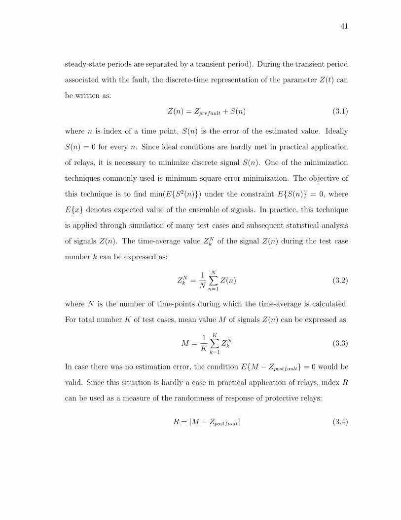
steady-state periods are separated by a transient period). During the transient period

associated with the fault, the discrete-time representation of the parameter Z(t) can

be written as:

Z(n) = Zprefault + S(n) (3.1)

where n is index of a time point, S(n) is the error of the estimated value. Ideally

S(n) = 0 for every n. Since ideal conditions are hardly met in practical application

of relays, it is necessary to minimize discrete signal S(n). One of the minimization

techniques commonly used is minimum square error minimization. The objective of

this technique is to find min(ES2(n)) under the constraint ES(n) = 0, where

Ex denotes expected value of the ensemble of signals. In practice, this technique

is applied through simulation of many test cases and subsequent statistical analysis

of signals Z(n). The time-average value ZNk of the signal Z(n) during the test case

number k can be expressed as:

ZNk =

1

N

N∑

n=1

Z(n) (3.2)

where N is the number of time-points during which the time-average is calculated.

For total number K of test cases, mean value M of signals Z(n) can be expressed as:

M =1

K

K∑

k=1

ZNk (3.3)

In case there was no estimation error, the condition EM − Zpostfault = 0 would be

valid. Since this situation is hardly a case in practical application of relays, index R

can be used as a measure of the randomness of response of protective relays:

R = |M − Zpostfault| (3.4)

42

G. Conclusion

The material covered in this chapter explained the sensitivity of the protection system

to signal distortions. First, basic elements and functions of the protection system

were described. It was shown that protection system is complex, both in elements

and functions. A simple method was used to demonstrate sensitivity of IEDs to

distortions. Since sensitivity varies depending on the amount of distortion, possible

negative impacts were discussed and illustrated. The primary cause of sensitivity of

protection system to input signal distortions was explained (random nature of the

protection system response).

The conclusion of the chapter is that protection system is sensitive to signal dis-

tortions. This sensitivity is not negligible. It was shown that signal distortion may

lead to protection misoperation, such as delayed trips and failures to trip. There-

fore, methodology for evaluation of the mentioned influence is necessary, in order to

correctly identify all situations that could lead to unacceptable protection response.

This conclusion presents incentive for development of a methodology for the

mentioned evaluation. This methodology, as well as associated criteria, is dealt with

in the next chapter.

43

CHAPTER IV

EVALUATION OF THE INFLUENCE OF SIGNAL DISTORTIONS

A. Introduction

Evaluation of relay performance is necessary in order to properly identify all the

situations when protection system may miss-operate, operate with unacceptably low

selectivity or unacceptably long operational time. This identification can help prevent

possible future misoperations. Other benefits of the mentioned evaluation include

overall improvement of protection schemes.

This chapter defines a set of criteria that can be used for numerical evaluation

of the protection system performance. Numerical evaluation means that criteria is

expressed quantitatively. Measuring and decision making algorithm are separate el-

ements of protection IEDs (see Chapter III). Therefore, criteria for the mentioned

algorithms is defined separately.

A new methodology for evaluation is also defined in this chapter. The definition

is summarized by answers to several crucial questions. Main contribution of the new

methodology is the combined approach to the evaluation. Currently, methodologies

for performance evaluation of instrument transformers and the protection system

exist. The new methodology, presented here, combines the mentioned two types

of methodologies, to evaluate the impact of instrument transformers on protection

system performance.

B. Shortcomings of the Existing Performance Criteria

Currently, there are many informal criteria that categorize the response of protection

IEDs. A typical criteria (that can be found in literature) classifies the protection

44

operation in the following classes [2]:

1. Correct

• As planned

• Not as planned or expected

2. Incorrect, either failure to trip or false tripping

• Not as planned or wanted

• Acceptable for the particular situation

3. No conclusion

Even though such a performance characterization can be useful, it suffers from certain

shortcomings:

• The classes are too broad in certain situations. For example, performances

of two protection devices that both properly detected a fault, but operated

with different time delays, can both be classified as correct. The are no means

within the mentioned class to indicated the difference in performance between

the two devices. Field experience has showed that such difference may cause

miss-coordination of the protection scheme [26].

• Classes are defined using intuitive terms, such as “planned” or “wanted”. De-

pending on the circumstances, these terms may vary greatly (e.g. “as planned”

operation may encompass a broad range of correct operations, where some of

these correct operations may be bordering with incorrect operations, as in the

case of overcurrent protection exposed to low-current faults that produce very

long operational time). Also, in certain situations it may prove hard to clearly

45

state limits between the terms. An example of such a situation is when a dis-

tance protection IED clears a fault near the end of zone 1, with unplanned time

delay close to planned time delay for faults in zone 2.

• The classification does not give any information about the reasons why the pro-

tection system operated in a certain manner. This brings out the fact that such

a scale is focused primarily on the link between the cause (fault, disturbance,

etc.) and the effect (protection system response), without taking into account

the processes taking places during the derivation of the protection response.

The above shortcomings make the mentioned performance criteria a poor choice for

evaluation of the influence of signal distortions on protection system performance.

In order to evaluate this influence accurately, a new evaluation criteria needs to be

defined, that will alleviate the mentioned shortcomings.

C. Criteria Based on the Measuring Algorithm

1. Time Response

Measuring algorithm traces a specific feature of the input signal (e.g. amplitude of a

sinusoidal waveform) [16]. That specific feature is called the measured value. Mea-

sured value is usually constant during the steady-state. However, transient periods

of the input signal cause significant fluctuations in the measured value within very

small time-intervals. Fluctuations can be illustrated by time response of a measuring

algorithm. Typical time response of a measuring algorithm is shown in Fig. 26. This

time response represents amplitude of a fault current signal (phase-to-ground fault),

where fault (event) occurs at 0.05 s.

Objective of the measuring algorithm is to capture all measured value fluctuations

with best possible accuracy. Performance indices can evaluate to what extent is this

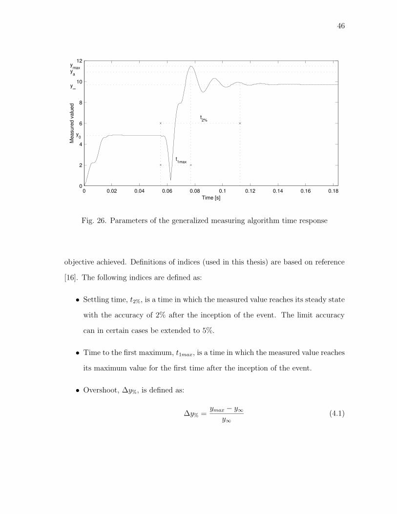
46

0 0.02 0.04 0.06 0.08 0.1 0.12 0.14 0.16 0.180

2

4

6

8

10

12

ya

ymax

y∞

t1max

t2%

Time [s]

Mea

sure

d va

lued

y0

Fig. 26. Parameters of the generalized measuring algorithm time response

objective achieved. Definitions of indices (used in this thesis) are based on reference

[16]. The following indices are defined as:

• Settling time, t2%, is a time in which the measured value reaches its steady state

with the accuracy of 2% after the inception of the event. The limit accuracy

can in certain cases be extended to 5%.

• Time to the first maximum, t1max, is a time in which the measured value reaches

its maximum value for the first time after the inception of the event.

• Overshoot, ∆y%, is defined as:

∆y% =ymax − y∞

y∞(4.1)

47

• Normalized error index, enorm, is defined as:

enorm =1

M · (y∞ − y0)

L+M∑

k=L

(

y(k) − ya

)

(4.2)

Index enorm is computed in the window of M samples starting from the L-th sample.

The reasons for the use of M-sample window is that some decision making algorithms

use transient monitors to postpone derivation of the output signal. This is reflected

in the choice of the value of L. When transient monitor is used, performance of the

measuring algorithm is of interest only after the transient period has passed. In case

the influence of the transient monitor needs to be neglected, L should be set to 1.

2. Frequency Response

Measuring algorithms in protective IEDs are designed to estimate a feature of a

harmonic component at specified frequency. In the United States, the frequency har-

monic is 60 Hz (in Europe, it is 50 Hz). To be able to correctly identify the mentioned

harmonic, other frequencies components should be suppressed during measurement.

However, small variations of specified frequency (60 Hz) are possible in power systems.

Because of this, measuring algorithms usually act as narrow band-pass filters.

Spectral content of a signal, with amplitude shown in Fig. 26, is given in Fig. 27.

Figure contains a portion of the spectrum around 60 Hz (since this is the frequency

of interest). This spectral content Yactual is the frequency response of the actual

measuring algorithm. Performance indices, that measure how much this response is

different from the ideal (band-pass filter) response Yideal can be defined. Definitions

of indices (used in this thesis) are based on reference [16]. The following indices are

defined:

48

0

0.5

1

1.5

Frequency [Hz]

Yac

tual

[p.u

.]

40 45 50 55 60 65 70 75 800

0.5

1

1.5

Frequency [Hz]

Yid

eal [p

.u.]

Fig. 27. Frequency response of the actual and the ideal measuring algorithm

• Gain for DC component, FRDC , is defined as:

FRDC =Yactual(0)

Yactual(60)(4.3)

• Aggregated index F , is defined as:

F =1

f2 − f1

∫ f2

f1

|Yideal(f) − Yactual(f)| df (4.4)

Even thought indices for time and frequency response are based on reference [16],

contribution of this thesis lies in software implementation of those indices and their

subsequent use for evaluation of influence of instrument transformers (while in refer-

ence [16] their use is confined to evaluation of relay performance).

49

D. Criteria Based on the Decision Making Algorithm

Decision making algorithm is supplied with the measured signals by the measuring

algorithm. By processing the measured signals, decision making algorithm derives the

final output. Final output may take one of the several forms. Examples are trip signal

(binary signal), fault location (numerical value) and power measurement (continuous

or discrete real signal). Based on the context of the output signal, evaluation criteria

for the decision making algorithm can be defined. The definitions developed in refer-

ences [14], [15] are the good starting point. Extending those definitions, reference [16]

proposes a more compact form of the decision making algorithm performance index:

J = C · P0 + (1 − C) · P1 + A · ttrip (4.5)

where C is an arbitrary factor defining the relative importance of the missing opera-

tions and false trippings, A is an arbitrary scaling factor defining the importance of

fast reaction time, P0,P1 are percentages of false trippings and missing operations,

respectively [14], [15], ttrip is the average tripping time. The lower the index J , the

better the relay performance. In this thesis, a different relay performance index is

defined and used:

• Selectivity, s, defined as:

s =N1 + N0

N(4.6)

where N1 denotes number of correct trip signals issued, N0 denotes number of

correct trip restraints and N is the total number of exposures. In ideal case

N = N1 + N0.

• Average tripping time, t, defined as time between fault inception and issuing of

trip signal.

50

E. Calculation of Performance Indices

While performance indices, defined in previous sections, may seem simple, their cal-

culation, based on realistic signals, can be quite involved. One major issue that

needs to be investigated further is the overshoot. Definition supplied in section C is

valid for any input signal. However, implementation of that definition needs further

clarification.

Depending on the input signal, measured value may have different shapes. Four

shapes that are often found in signals from power networks are shown in Fig. 28.

These four shapes are useful in illustrating calculation of the overshoot. In the figure,

abscissa presents time (in [s]), while time-points where an event occurs (that leads

to change of measured value) are marked with a vertical dashed line. As can be

seen, measured values in Figs. 28(a) and (b) actually do not show any overshoot. In

Figs. 28(c) and (d) the overshoot is present. The two overshoots differ significantly,

though. In figure (c) the overshoot is result of a drop of measured value from pre-event

value to post-event value. The overshoot is negative. In figure (d) the overshoot re-

sults from a rise of the measured value. This leads to a positive overshoot. Because of

this overshoot behavior, it is necessary to have the means to differ between overshoot

types (when calculating performance indices). Simple way of differentiating between

the overshoots is to compare the pre-event and post-event measured values. In the

case the pre-event is greater than the post-event value, the overshoot is found as the

minimum of the measured value, after the event occurrence. If the pre-event value is

smaller than the post-event, the overshoot is found as the maximum of the measured

value, again, after event occurrence. Another issue is the fluctuation of steady-state

value. After the 2% setting time, measured value (depending on type of measuring

algorithm) often oscillates around certain value. For this reason, parameter yinf (see

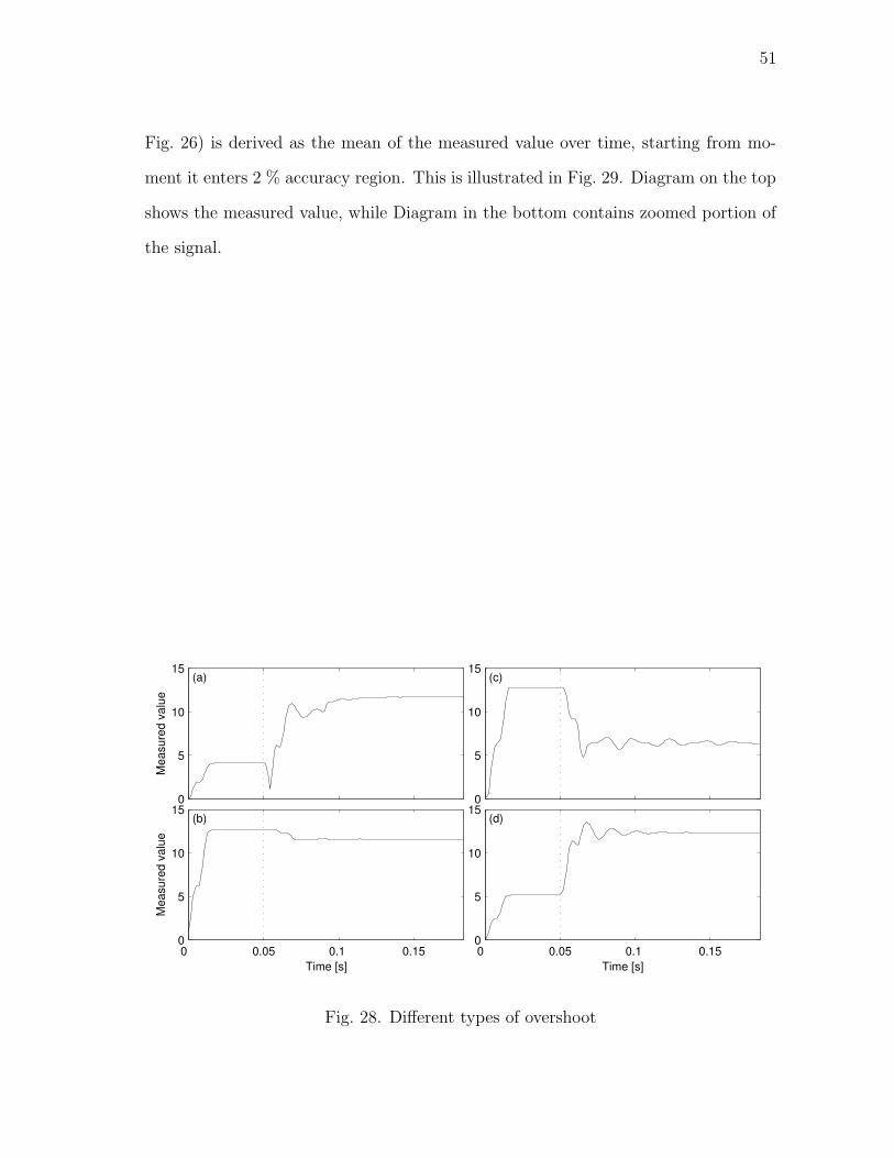
51

Fig. 26) is derived as the mean of the measured value over time, starting from mo-

ment it enters 2 % accuracy region. This is illustrated in Fig. 29. Diagram on the top

shows the measured value, while Diagram in the bottom contains zoomed portion of

the signal.

0

5

10

15

(a)

Mea

sure

d va

lue

(a)

0 0.05 0.1 0.150

5

10

15

Time [s]

Mea

sure

d va

lue

(b)

0

5

10

15

(c)

(c)

0 0.05 0.1 0.150

5

10

15

Time [s]

(d)

Fig. 28. Different types of overshoot

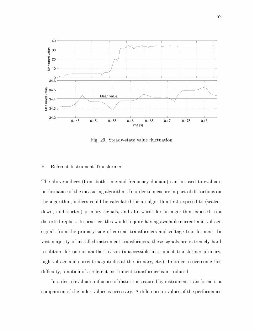
52

0

10

20

30

40

(a) Fluctuations of steady−state value after the settling time

Mea

sure

d va

lue

0.145 0.15 0.155 0.16 0.165 0.17 0.175 0.18 34.2

34.3

34.4

34.5

34.6

Time [s]

Mea

sure

d va

lue

Mean value

Fig. 29. Steady-state value fluctuation

F. Referent Instrument Transformer

The above indices (from both time and frequency domain) can be used to evaluate

performance of the measuring algorithm. In order to measure impact of distortions on

the algorithm, indices could be calculated for an algorithm first exposed to (scaled-

down, undistorted) primary signals, and afterwards for an algorithm exposed to a

distorted replica. In practice, this would require having available current and voltage

signals from the primary side of current transformers and voltage transformers. In

vast majority of installed instrument transformers, these signals are extremely hard

to obtain, for one or another reason (unaccessible instrument transformer primary,

high voltage and current magnitudes at the primary, etc.). In order to overcome this

difficulty, a notion of a referent instrument transformer is introduced.

In order to evaluate influence of distortions caused by instrument transformers, a

comparison of the index values is necessary. A difference in values of the performance

53

indices between:

1. Measuring algorithm exposed to signals supplied by a referent instrument trans-

former

2. Measuring algorithm exposed to signals supplied by instrument transformer

under investigation

is an indicator of the influence of a particular instrument transformer on the measuring

algorithm performance. The main idea behind this concept is that referent instrument

transformer can be regarded as ideal, and therefore, deliver exact signals from the

primary side. This is, of course, impossible to achieve with realistic transformers.

However, it may not be necessary to demand such high performance from referent

instrument transformer. Referent instrument transformer can be any instrument

transformer which performance has two characteristics:

1. Performance is known, meaning that it has been proven in field application or

laboratory testing as accurate

2. Performance is stable, meaning that it has been proven over some period of

time to be not deteriorating

An example of one such instrument transformer would be novel, optical current trans-

ducer. Its laboratory testing and preliminary field application point toward both

characteristics. The meaning and the interpretation of the difference depends on the

choice of the particular indices used as criteria. It is possible to choose a particular

set of indices to target evaluation of influence of a particular instrument transformer

characteristic. For example, if the influence of the transient response (see Chapter II)

needs to be evaluated, a set of criteria indices may consist of:

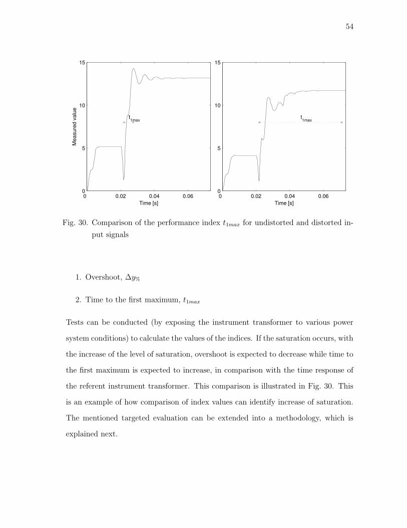
54

0 0.02 0.04 0.060

5

10

15

t1max

Time [s]0 0.02 0.04 0.060

5

10

15

t1max

Time [s]

Mea

sure

d va

lue

Fig. 30. Comparison of the performance index t1max for undistorted and distorted in-

put signals

1. Overshoot, ∆y%

2. Time to the first maximum, t1max

Tests can be conducted (by exposing the instrument transformer to various power

system conditions) to calculate the values of the indices. If the saturation occurs, with

the increase of the level of saturation, overshoot is expected to decrease while time to

the first maximum is expected to increase, in comparison with the time response of

the referent instrument transformer. This comparison is illustrated in Fig. 30. This

is an example of how comparison of index values can identify increase of saturation.

The mentioned targeted evaluation can be extended into a methodology, which is

explained next.

55

G. Definition of the New Methodology

New methodology for evaluation is intended to improve existing practice. Key ele-

ments of the methodology definition are:

1. Establishing reasons why evaluation is necessary

2. Proposing criteria for evaluation

3. Defining procedure and identifying tools for evaluation

4. Interpretation of evaluation results

The key elements are summarized in the form of questions and answers.

Why is evaluation of influence of instrument transformers on IEDs necessary

and important ? There are two main reasons:

1. Instrument transformers are known to distort signals coming from the primary

side. At present, there is no generally successful way to altogether eliminate

distortions. Main reasons for distortions are instrument transformer design

characteristics, which are inherent to instrument transformers. Characteristics

and their impact on distortions are discussed in the Chapter II.

2. Protection IEDs are sensitive to signal distortions. This sensitivity can, in cer-

tain cases, cause misoperation of IEDs. Since distortions originate inside instru-

ment transformers, we can regard distortions as direct influence of instrument

transformers. Negative impacts of distortions are discussed in Chapter III.

How can the influence of instrument transformers be measured ? The influence

can be measured by defining criteria in a context of the protection system functions.

The evaluation can be done by comparing performance of the functions in two cases:

56

1) functions exposed to signals supplied by a referent instrument transformer, 2)

functions exposed to signals supplied by instrument transformers under investigation.

Difference in numerical values of the performance indices are a clear and effective

indicator of the mentioned influence. This concept of comparison is discussed in

section F.

What are the means for quantifying the influence (finding numerical values) ?

There are well-defined performance indices for various protection elements and func-

tions in the literature [13]-[16]. These indices can be adapted to serve as a quantitative

indicator of the influence of the instrument transformers on the protection function

performance. Practical definition of the criteria, taken from [16], is given in sections

C and D. It is important to note again that, index values itself are NOT an indicator

of the mentioned influence; rather, the DIFFERENCE in values is the indicator.

What is the best procedure for finding the quantitative values of the instrument

transformer influence ? The best procedure is a statistical analysis of the performance

of the protection system. Statistical methods can be used as a tool to quickly and

efficiently sort through large number of test cases, and derive values of indices. The

basis of the statistical analysis methodology are available in the literature [16]. One

particular statistical method will be developed later in the thesis.

What is the meaning of the quantitative values ? Quantitative values are sta-

tistical indicators of the function performance (to what extent the protection system

performance was satisfactory ?). The difference in the numerical values for the cases

defined in the first question is a numerical indicator of the influence of instrument

transformers on the function performance.

57

H. Conclusion

This chapter introduced criteria for evaluation of the signal distortions on IEDs. First,

the reasons for doing so were discussed. Separate criteria was defined for different

elements of IEDs. It was shown how particular distortions, caused by certain instru-

ment transformer characteristics, can be targeted for evaluation. One application of

this targeting, methodology for evaluation, was also discussed.

The conclusion of the chapter is that presented criteria can be used as an effective

and meaningful mean for identification of influence of distortions. The criteria is based

on quantitative values, which means that evaluation is exact and comprehensive.

Based on this, a new methodology for evaluation was defined. They key elements of

the methodology are: 1) reasons why evaluation is necessary, 2) criteria for evaluation,

3) tools for evaluation, 4) interpretation of evaluation results. All elements were

explained. It was concluded that the new methodology presents a systematic and

exhaustive approach to the problem posed in the first, introductory chapter. Based

on the definition of the new methodology, a simulation approach will be presented in

the next chapter.

58

CHAPTER V

EVALUATION THROUGH MODELING AND SIMULATION

A. Introduction

The performance indices, defined in previous chapter, may be calculated by analyzing

output signals of IEDs. Outputs of IEDs are triggered by certain input signals.

Options for generating IED inputs to obtain output signals are:

• Field-recorded data

• Signals obtained from simulations

If the field recorded data contains all the signals necessary for calculation of

performance indices, then the indices can be derived directly from the data. What

are the necessary signals depends on the nature of indices. Since large number of

signal cases is desirable (field recordings may not be sufficient), the simulation often

proves to be a more practical approach.

This chapter describes evaluation through modelling and simulation. Simulation

approach will be addressed first. Next, power network, instrument transformer, and

IED models will be listed and described. The reasons for their selection will also

be discussed. Afterwards, scenarios for simulations will be defined. The material

presented in this chapter is a background for software implementation, presented in

the next chapter.

B. Simulation Approach

As mentioned in the introduction, IED model responses are initiated by input signals

derived by simulating signals corresponding to various power system events (faults,

59

disturbances, etc.). The input signals, derived from simulating a given event, con-

stitute a single exposure [14]. In this thesis, exposure is defined as a 3-phase set of

current and voltage waveforms, that represent given power system event. An example

of exposure is shown in Fig. 18 (in Chapter III). The fault for which the exposure

was captured is a phase-A-to-ground (AG) fault, without phase-to-ground resistance.

As can be seen in the figure, exposure contains steady-state waveforms, followed by

a transient after the inception of fault. Signals, that make an exposure, trigger IED

model to perform certain operations, and to issue certain output signals, if necessary.

Correct IED model response may be either issuing a trip signal, or restraining from

tripping.

Objective of the simulation is to subject IED models to a large number of expo-

sures and record IED responses. Afterwards, the recorded data is used for derivation

of performance indices. The simulation procedure can be summarized in the following

steps :

1. Create a database of exposures by simulating events using power network model

2. Feed the exposures into the models of instrument transformers and IEDs

3. Record necessary IED output signals (from both the measuring and decision

making algorithm)

The steps are illustrated in Fig. 31. Shaded elements produce output that is

stored for future use. Two main elements of a simulation are:

1. Models

2. Scenarios

In the following sections, models used in simulation will be described. Importance of

proper selection of models will be emphasized. Afterwards, scenarios will be defined.

60

Power Network Model

Exposures Recorded

Model Responses

IT, IED Models Scenarios

Step 1 Step 2 Step 3

Fig. 31. Steps of the simulation procedure

C. Simulation Models

1. Power Network Model

Model of the power network should accurately capture dynamic characteristic of dis-

turbances, including faults. Network interconnections should be included as Thevenin

equivalents. Power network model selected for simulations is a 9-bus, 11-lines, 345

kV power system section. Fig. 32 shows one-line diagram of the network. The model

was developed according to example given in reference [31]. The example is based on

a realistic power network section.

2. Current Transformer Models

Models of instrument transformers should include features that accurately represent

their characteristics, discussed in Chapter II. Four current transformer models were

chosen for evaluation. All the models have the same general equivalent circuit, shown

in Fig. 33. The circuit is proposed as suitable for simulation in the literature [8], [10],

[26].

Differences between models are in their parameters. Parameters were chosen to

be representative of current transformer characteristics that can cause distortions.

Saturation, the major cause of distortion, is mainly dependent on the current trans-

former burden and V-I characteristic of the electromagnetic core. Therefore, two

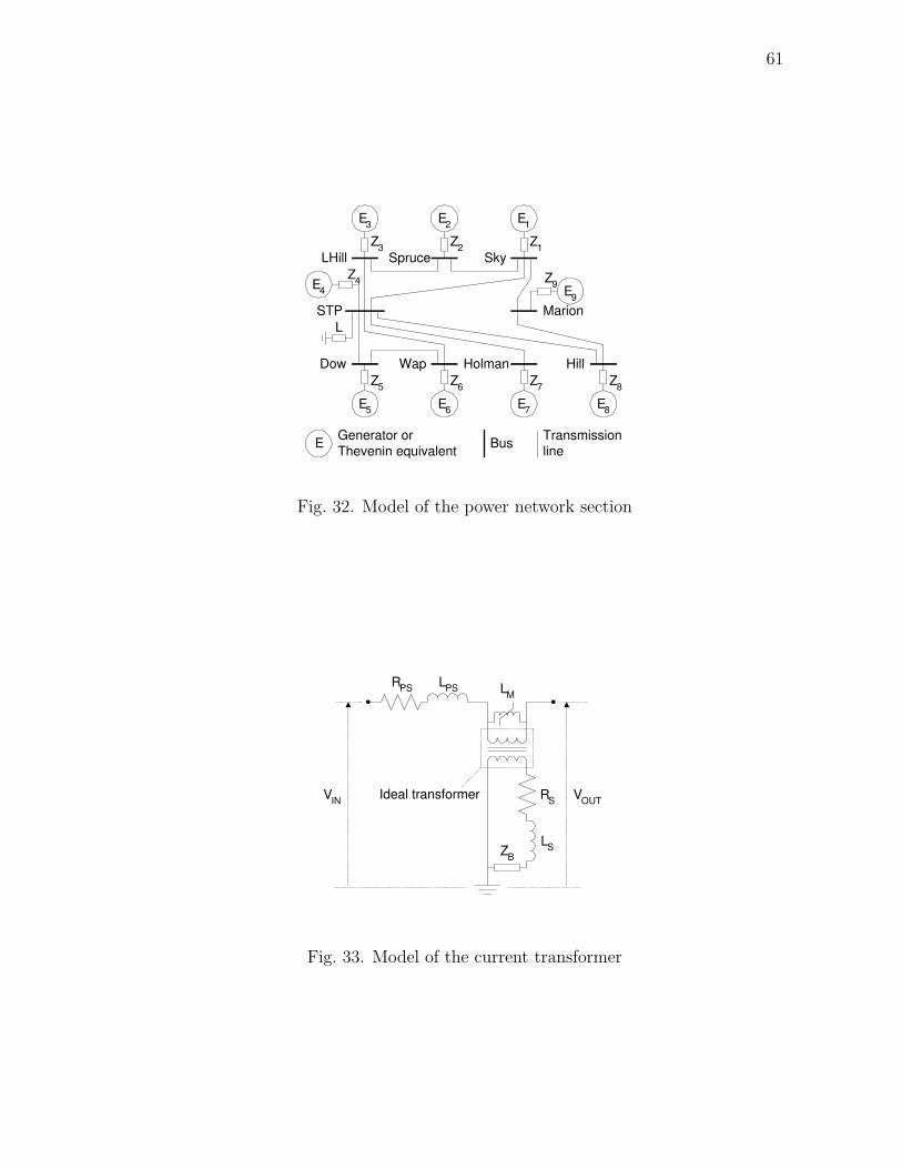
61

LHill Sky

E 3

Z 3

E 2

Z 2

E 1

Z 1

Z 4 E 4 Z 9

E 9

Dow Wap Holman Hill

E 5

Z 5

E 6

Z 6

E 7

Z 7

E 8

Z 8

Spruce

STP Marion L

E Generator or Thevenin equivalent Bus Transmission

line

Fig. 32. Model of the power network section

R S

L S Z B

Ideal transformer

R PS L PS L M

V IN V OUT

Fig. 33. Model of the current transformer

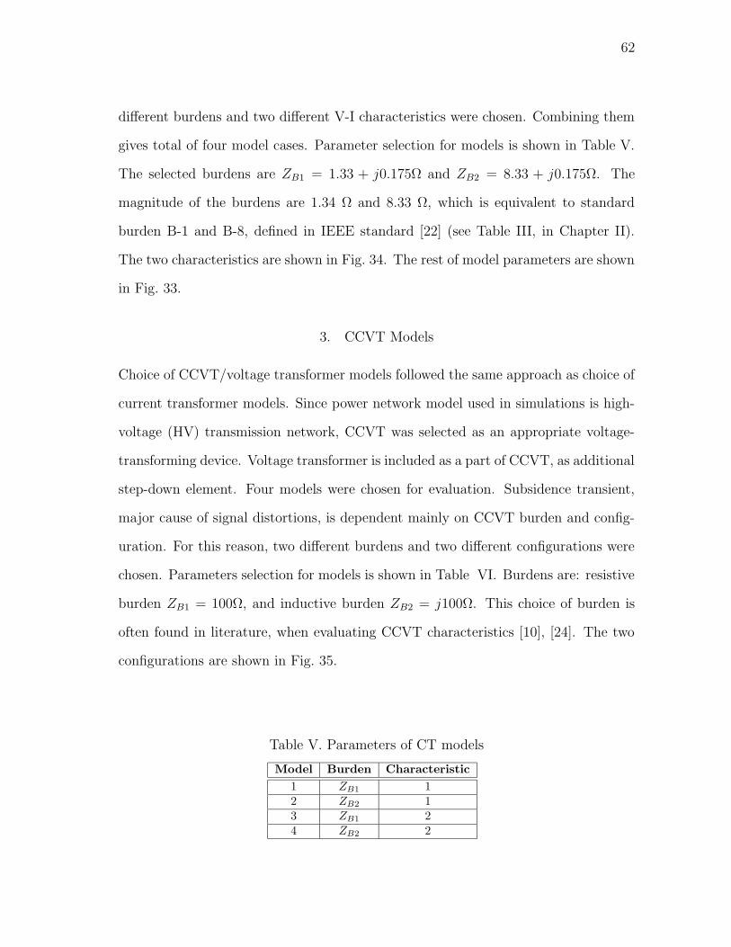
62

different burdens and two different V-I characteristics were chosen. Combining them

gives total of four model cases. Parameter selection for models is shown in Table V.

The selected burdens are ZB1 = 1.33 + j0.175Ω and ZB2 = 8.33 + j0.175Ω. The

magnitude of the burdens are 1.34 Ω and 8.33 Ω, which is equivalent to standard

burden B-1 and B-8, defined in IEEE standard [22] (see Table III, in Chapter II).

The two characteristics are shown in Fig. 34. The rest of model parameters are shown

in Fig. 33.

3. CCVT Models

Choice of CCVT/voltage transformer models followed the same approach as choice of

current transformer models. Since power network model used in simulations is high-

voltage (HV) transmission network, CCVT was selected as an appropriate voltage-

transforming device. Voltage transformer is included as a part of CCVT, as additional

step-down element. Four models were chosen for evaluation. Subsidence transient,

major cause of signal distortions, is dependent mainly on CCVT burden and config-

uration. For this reason, two different burdens and two different configurations were

chosen. Parameters selection for models is shown in Table VI. Burdens are: resistive

burden ZB1 = 100Ω, and inductive burden ZB2 = j100Ω. This choice of burden is

often found in literature, when evaluating CCVT characteristics [10], [24]. The two

configurations are shown in Fig. 35.

Table V. Parameters of CT models

Model Burden Characteristic

1 ZB1 12 ZB2 13 ZB1 24 ZB2 2

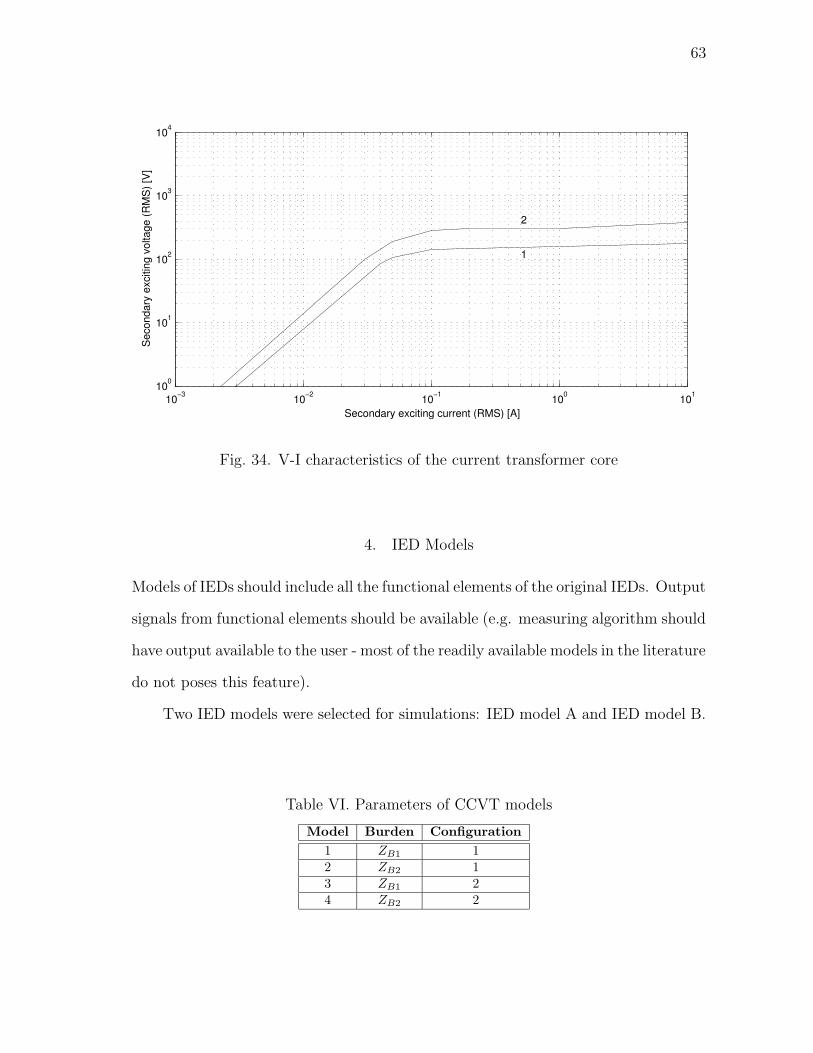
63

10−3 10−2 10−1 100 101100

101

102

103

104

Secondary exciting current (RMS) [A]

Sec

onda

ry e

xciti

ng v

olta

ge (R

MS

) [V

]

1

2

Fig. 34. V-I characteristics of the current transformer core

4. IED Models

Models of IEDs should include all the functional elements of the original IEDs. Output

signals from functional elements should be available (e.g. measuring algorithm should

have output available to the user - most of the readily available models in the literature

do not poses this feature).

Two IED models were selected for simulations: IED model A and IED model B.

Table VI. Parameters of CCVT models

Model Burden Configuration

1 ZB1 12 ZB2 13 ZB1 24 ZB2 2

64

Configuration 1

Configuration 2

R C L C

C C

R P L P R S L S

C F

R F

L F

R B

C 1

C 2 L M R M C P

V IN

V OUT

R C L C

C C

R P L P R S L S

C F

R F

L F

R B

C 1

C 2 L M R M

C P V IN

V OUT

Fig. 35. Configurations of CCVT models

Model A represent a line overcurrent protection relay. The model offers the following

features:

• Three-phase directional instantaneous overcurrent relaying, if used as a primary

protection

• Three-phase time overcurrent relaying, if used as a backup protection

The elements and flowchart of model A are shown in Fig. 36. Elements of the

IED model A are:

• Measuring algorithm performs extraction of current and voltage phasor from

the signals supplied by instrument transformers. Extraction is performed by

65

Measuring Algorithm

Overcurrent Element Logic

Voltage signals

Current signals Trip

Database of IED responses

Fig. 36. Elements and the flowchart of the IED model A

Fourier algorithm. The phasor values are multiplexed together and sent to

overcurrent element.

• Overcurrent element consists of three sub-elements, each providing protection

by a certain operating principle. The sub-elements are:

1. Time overcurrent protection. This protection provides fast operation time

for high fault currents, and slow operation when light currents are detected.

This results in inverse time characteristic.

2. Ground time overcurrent protection. This protection operates when a fault

involving ground is detected. It uses the same type of characteristics as

the time overcurrent protection.

3. Directional protection. This protection is designed to operate for faults in

a certain direction. This protection element uses direction of the flow of

the current or power to determine whether a fault is in the direction of

protected line.

• Logic element applies logic functions (AND,OR) on the assertion signals pro-

duced by the protection element and operates the circuit breakers only when a

fault current is sufficiently high and when the fault is detected in the direction

66

of interest. Otherwise, logic element restraints the relay from asserting the trip

signal.

Output signals of IED model A are available for capturing. They are recorded

to database of IED responses, together with trip signals. Settings for the IED model

A are:

• Nominal current on input of IED model is In=5 A.

• Pickup current is set to twice the nominal value: Ipickup=10 A.

• Extra inverse time-current characteristic was used. This characteristic is defined

as [32]:

toperate =13.5 · k

In − 1(5.1)

Time-parameter k was chosen as: k=0.02. This characteristic allows for efficient

distinction between near-end and far-end faults on the protected line Sky-STP,

because of the parameters of the transmission line (length and impedance).

More on the selected inverse-time characteristic can be found in reference [32].

The plot of characteristic is shown in Fig. 37.

IED model B represents a transmission line distance (impedance) protection

relay. Protection features implemented in the model are [29]:

• Three separate MHO forward sensing zones for multi-phase faults

• Three separate quadrilateral forward sensing zones for phase to ground faults

• One MHO reverse sensing zone for multi-phase faults

• One quadrilateral reverse sensing zone for phase to ground faults

• Six separate MHO starters, one for each fault-measured loop

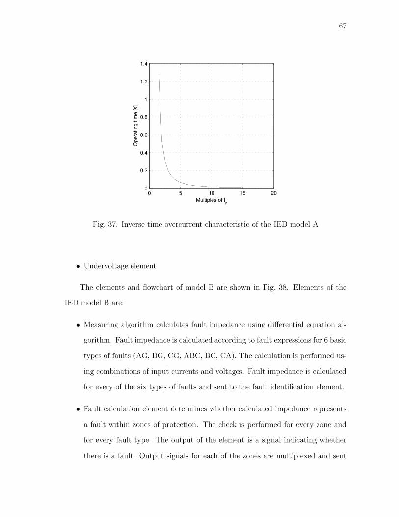
67

0 5 10 15 200

0.2

0.4

0.6

0.8

1

1.2

1.4

Multiples of In

Ope

ratin

g tim

e [s

]

Fig. 37. Inverse time-overcurrent characteristic of the IED model A

• Undervoltage element

The elements and flowchart of model B are shown in Fig. 38. Elements of the

IED model B are:

• Measuring algorithm calculates fault impedance using differential equation al-

gorithm. Fault impedance is calculated according to fault expressions for 6 basic

types of faults (AG, BG, CG, ABC, BC, CA). The calculation is performed us-

ing combinations of input currents and voltages. Fault impedance is calculated

for every of the six types of faults and sent to the fault identification element.

• Fault calculation element determines whether calculated impedance represents

a fault within zones of protection. The check is performed for every zone and

for every fault type. The output of the element is a signal indicating whether

there is a fault. Output signals for each of the zones are multiplexed and sent

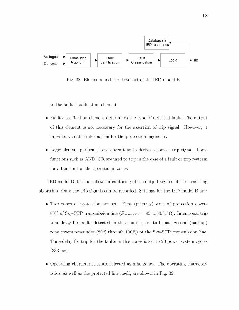
68

Database of IED responses

Measuring Algorithm

Fault Identification Logic

Voltages

Currents Trip Fault

Classification

Fig. 38. Elements and the flowchart of the IED model B

to the fault classification element.

• Fault classification element determines the type of detected fault. The output

of this element is not necessary for the assertion of trip signal. However, it

provides valuable information for the protection engineers.

• Logic element performs logic operations to derive a correct trip signal. Logic

functions such as AND, OR are used to trip in the case of a fault or trip restrain

for a fault out of the operational zones.

IED model B does not allow for capturing of the output signals of the measuring

algorithm. Only the trip signals can be recorded. Settings for the IED model B are:

• Two zones of protection are set. First (primary) zone of protection covers

80% of Sky-STP transmission line (ZSky−STP = 95.4 6 83.81Ω). Intentional trip

time-delay for faults detected in this zones is set to 0 ms. Second (backup)

zone covers remainder (80% through 100%) of the Sky-STP transmission line.

Time-delay for trip for the faults in this zones is set to 20 power system cycles

(333 ms).

• Operating characteristics are selected as mho zones. The operating character-

istics, as well as the protected line itself, are shown in Fig. 39.

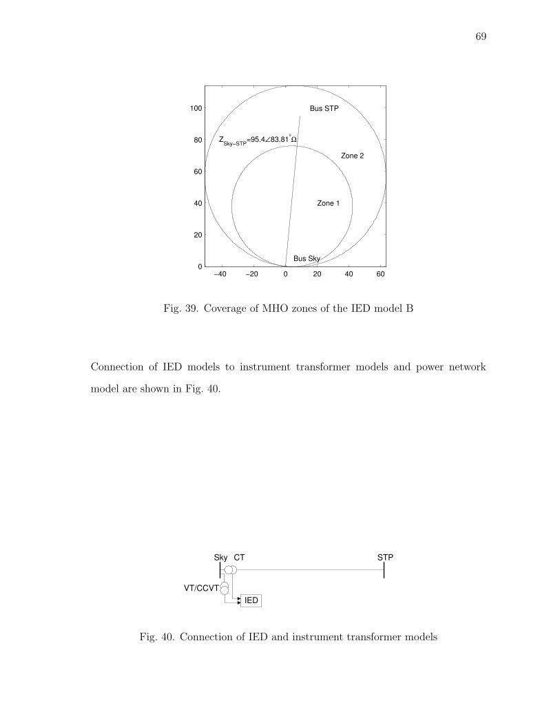
69

−40 −20 0 20 40 600

20

40

60

80

100

ZSky−STP

=95.4∠83.81°Ω

Bus Sky

Bus STP

Zone 1

Zone 2

Fig. 39. Coverage of MHO zones of the IED model B

Connection of IED models to instrument transformer models and power network

model are shown in Fig. 40.

Sky STP

IED

CT

VT/CCVT

Fig. 40. Connection of IED and instrument transformer models

70

D. Simulation Scenarios

Events are organized according to simulation scenarios. The scenarios definition con-

sists of:

1. Timeline of events

2. Features of events

Timeline defines time points when each of the events starts and when it finishes.

Event is usually modelled by a sequence of switching of power network circuit breakers.

Switchings allow for a modification of network topology, thus simulating faults and

disturbances. The events are characterized by their features. Examples of features

are: location of the event along the transmission line, associated resistances (such as

ground or line-to-line resistances), point-on-wave of fault inception and so on.

In this thesis, two scenarios were defined, for two models of IEDs. The events

were selected to emulate situations when the influence of instrument transformers can

be critical.

Different scenarios were defined for IED models A and B, as shown in Tables

VII and VIII. In the case of IED model A, faults were simulated both in forward

and backward zone of protection. IED model is expected to operate for faults in the

forward zone of protection, while it is expected to restrain from operating (issuing a

trip signal) for faults in the backward zone of protection. In the case of IED model

B, faults were simulated in zones 1 and 2. Fault locations were chosen to test IED

response of both primary and backup zone of protection.

Three types of faults are simulated: phase-to-ground (AG) and phase-to-phase

(BC) faults, as well as their combination (ABCG). The model should be transparent

to different types of faults (considering selectivity and operational time). Every fault

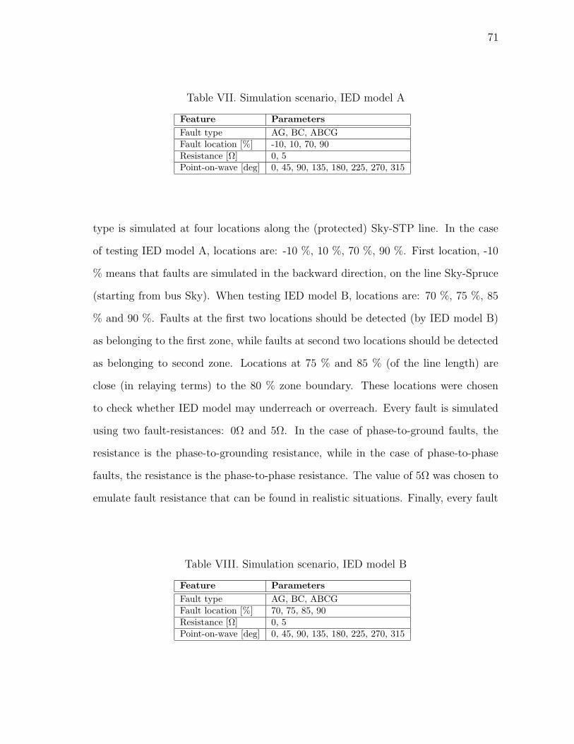
71

Table VII. Simulation scenario, IED model A

Feature Parameters

Fault type AG, BC, ABCGFault location [%] -10, 10, 70, 90Resistance [Ω] 0, 5Point-on-wave [deg] 0, 45, 90, 135, 180, 225, 270, 315

type is simulated at four locations along the (protected) Sky-STP line. In the case

of testing IED model A, locations are: -10 %, 10 %, 70 %, 90 %. First location, -10

% means that faults are simulated in the backward direction, on the line Sky-Spruce

(starting from bus Sky). When testing IED model B, locations are: 70 %, 75 %, 85

% and 90 %. Faults at the first two locations should be detected (by IED model B)

as belonging to the first zone, while faults at second two locations should be detected

as belonging to second zone. Locations at 75 % and 85 % (of the line length) are

close (in relaying terms) to the 80 % zone boundary. These locations were chosen

to check whether IED model may underreach or overreach. Every fault is simulated

using two fault-resistances: 0Ω and 5Ω. In the case of phase-to-ground faults, the

resistance is the phase-to-grounding resistance, while in the case of phase-to-phase

faults, the resistance is the phase-to-phase resistance. The value of 5Ω was chosen to

emulate fault resistance that can be found in realistic situations. Finally, every fault

Table VIII. Simulation scenario, IED model B

Feature Parameters

Fault type AG, BC, ABCGFault location [%] 70, 75, 85, 90Resistance [Ω] 0, 5Point-on-wave [deg] 0, 45, 90, 135, 180, 225, 270, 315

72

is simulated starting at 8 different fault inception moments (point-on-wave), covering

range of one 60 Hz cycle in 8 equal, consecutive time-steps. Total number of cases

generated for each of IED models is: 3 · 4 · 2 · 8 = 192.

E. Benefits and Limitations of the Simulation Approach

Simulation approach has distinctive benefits, as well as limitations, when compared

to different approaches, such as hardware testing. When deciding upon the use of the

simulation approach, both the limitations and benefits should be carefully considered.

Benefits of the simulation approach are:

• In the evaluation stages, problematic components of instrument transformers

can be identified using simulation approach. This is valid under assumption

that models of instrument transformers and protective relays are available for

evaluation.

• Simulation approach is a great tool for educational purposes. It provides a novel

insight into evaluation of influence of instrument transformers on internal com-

ponents of IEDs. This insight creates much better understanding of interaction

between instrument transformers and power system protection system.

Limitations of the simulation approach are:

• Evaluation of existing instrument transformers and IEDs is limited by the avail-

ability of models of devices. At present, there is only a small number of com-

mercial protective relay and instrument transformer models (in the available

literature). In other cases, models may exist but may not be readily available

to the user.

73

• Most of the commercial protective relays do not provide access to output sig-

nals of the measurement unit. Some commercial relays (e.g. SEL-321) provide

recordings of some internal measurements. The mentioned recording can be

used to derive some of the performance indices (allowing for at least partial use

of simulation approach).

F. Conclusion

This chapter described simulation approach to evaluation of influence of instrument

transformers. First, details about the approach, such as types of data and procedures

to be used, were discussed. The role of models was also addressed. Next, models of

power network, instrument transformers and IEDs were described. The reasons for

choice of models was explained. Elements and structure for each IED model were also

presented. Settings for IED models were defined. Afterwards, simulation scenarios

were defined. Event features of scenarios were selected to exacerbate possible critical

influence of instrument transformer models on IED models.

Conclusion of the chapter is that by proper choice of models, effective and mean-

ingful results can be obtained through simulation. An advantage of simulation ap-

proach over field collected data was pointed out: amount of data collected from field

recording can be insufficient for proper evaluation of influence of instrument trans-

formers. Therefore, simulation approach is a suitable mean for implementing the

evaluation methodology.

Material presented in this chapter is a theoretical background for the next chap-

ter. Next chapter describes software implementation of simulation approach: simula-

tion environment.

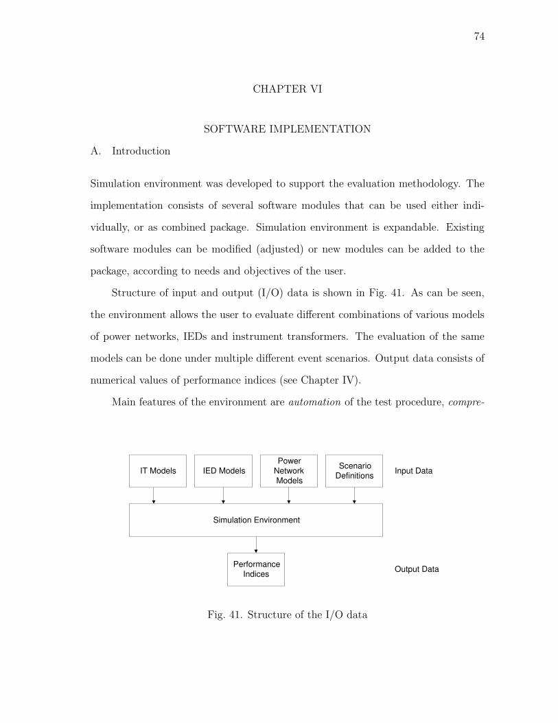
74

CHAPTER VI

SOFTWARE IMPLEMENTATION

A. Introduction

Simulation environment was developed to support the evaluation methodology. The

implementation consists of several software modules that can be used either indi-

vidually, or as combined package. Simulation environment is expandable. Existing

software modules can be modified (adjusted) or new modules can be added to the

package, according to needs and objectives of the user.

Structure of input and output (I/O) data is shown in Fig. 41. As can be seen,

the environment allows the user to evaluate different combinations of various models

of power networks, IEDs and instrument transformers. The evaluation of the same

models can be done under multiple different event scenarios. Output data consists of

numerical values of performance indices (see Chapter IV).

Main features of the environment are automation of the test procedure, compre-

IED Models Power

Network Models

Scenario Definitions IT Models

Simulation Environment

Performance Indices

Input Data

Output Data

Fig. 41. Structure of the I/O data

75

hensiveness of the results and flexibility of the use. Automation means that testing

is performed with a minimal user interaction (without any loss of accessibility or

modifiability of relevant simulation parameters). The comprehensiveness means a

sufficient number of test cases is always covered, while each case presents protection

system conditions with a sufficient number of parameters. Flexibility means: 1) differ-

ent instrument transformer and IED models can be integrated into testing, allowing

the user to test and compare influence of various instrument transformer versions

and designs, 2) results can be generated in the form of graphs and tables that can

be directly imported into various text processors, allowing the user to quickly and

efficiently analyze final results.

This chapter describes elements, structure and software implementation of the

simulation environment. Special attention is given to explaining I/O structures and

flowcharts of various elements. The reason for doing so is to give information to the

user who wishes to modify or expand the environment, or wishes to use data generated

by the environment in additional studies. User interface is also discussed.

B. Structure of the Simulation Environment

Main functional elements and flowchart of the environment are shown in Fig. 42.

There are three main elements:

1. Exposure generator

2. Exposure replayer

3. Statistical analyzer

Output of the environment are tables containing numerical values of performance

indices (see Chapters IV and V). In the process of derivation of mentioned indices,

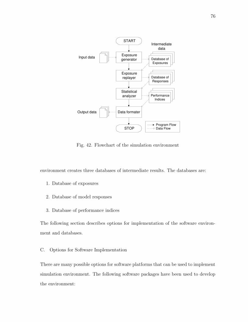
76

Exposure generator

Exposure replayer

Statistical analyzer

Data formater

START

STOP

Performance Indices

Database of Exposures

Database of Responses

Program Flow Data Flow

Input data

Output data

Intermediate data

Fig. 42. Flowchart of the simulation environment

environment creates three databases of intermediate results. The databases are:

1. Database of exposures

2. Database of model responses

3. Database of performance indices

The following section describes options for implementation of the software environ-

ment and databases.

C. Options for Software Implementation

There are many possible options for software platforms that can be used to implement

simulation environment. The following software packages have been used to develop

the environment:

77

• Alternative Transient Program (ATP) [23]. This program is a version of Electro-

magnetic Transient Program (EMTP). Purpose of ATP package is simulation of

transient waveforms associated with electromagnetic phenomena in power net-

works. Program also has the option of frequency analysis. ATP development

was continuous over the last 20 years. Contributors in development are inter-

national, while the coordinator is the Canadian/American ATP Users Group

(available online: www.emtp.org).

Input of ATP are text files, called scripts. Scripts consist of a list of power

network elements and their connections. Together, elements and connections

define a model of a network. Basic operation of ATP is calculation of variables

of interest (current and voltages), as functions of time. Variables of interest

are defined by the user. Calculation is based on solving differential equations

that describe behavior of system components in time domain. Trapezoidal rule

of integration is used for solving. There are two ways of determining initial

conditions: 1) initial steady-state (phasor) solution of the system model, 2)

initial values specified by the user (for some components).

Extensive library of power system component models is available in the cur-

rent version of ATP. Models include: rotating machines, transformers, surge

arresters, transmission lines, cables, etc. By combining mentioned components,

complex networks can be built. Additional feature of the program allows for

analysis of control systems, power electronics equipment and components with

nonlinear characteristics, such as arcs, corona and saturable electromagnetic

core. When simulating events, both symmetric and asymmetric disturbances

are allowed.

• Matlab [33]. The name Matlab stands for Matrix Laboratory. Matlab is a high-

78

Table IX. Implementation of the software environment

Package Usage

ATP Implementation of power network and instrument transformer modelsGeneration of exposure waveforms

Matlab Replaying of exposure waveformsStatistical analysis of IED model responsesCreation of output data tables

Simulink Implementation of IED modelsGeneration of IED response signals

performance language for technical computing. It represents the state-of-the-art

in software for matrix computation. One of the main parts of the program is

Matlab language. This language is a high-level matrix/array language, with

control flow statements, functions, data structures, input/output and object-

oriented programming features. Such a structure allows for creating large and

complex application programs using relatively simple instructions.

• Simulink [34]. Simulink is Matlab’s companion program. Its purpose is simulat-

ing nonlinear dynamic system models. Types of systems that can be modelled

using Simulink include linear, nonlinear, continuous-time, discrete-time, multi-

variable and multi-rate. Main feature of the program is attractive, easy-to-use

graphical user interface (GUI). This interface allows for building of models by

simply placing system components on the work sheet and specifying connections

between them. In order to simulate power network systems, Power Blockset can

be used [35]. This blockset is an additional library of system components that

model power network elements. Power blockset presents a specialized applica-

tion of Simulink.

Table IX gives an overview of implementation options for the software environment.

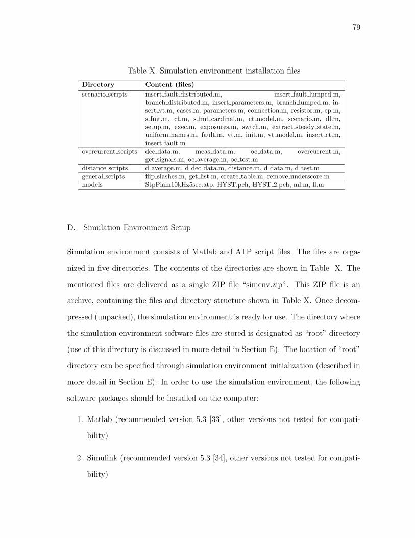
79

Table X. Simulation environment installation files

Directory Content (files)

scenario scripts insert fault distributed.m, insert fault lumped.m,branch distributed.m, insert parameters.m, branch lumped.m, in-sert vt.m, cases.m, parameters.m, connection.m, resistor.m, cp.m,s fmt.m, ct.m, s fmt cardinal.m, ct model.m, scenario.m, dl.m,setup.m, exec.m, exposures.m, swtch.m, extract steady state.m,uniform names.m, fault.m, vt.m, init.m, vt model.m, insert ct.m,insert fault.m

overcurrent scripts dec data.m, meas data.m, oc data.m, overcurrent.m,get signals.m, oc average.m, oc test.m

distance scripts d average.m, d dec data.m, distance.m, d data.m, d test.mgeneral scripts flip slashes.m, get list.m, create table.m, remove underscore.mmodels StpPlain10kHz5sec.atp, HYST.pch, HYST 2.pch, ml.m, fl.m

D. Simulation Environment Setup

Simulation environment consists of Matlab and ATP script files. The files are orga-

nized in five directories. The contents of the directories are shown in Table X. The

mentioned files are delivered as a single ZIP file “simenv.zip”. This ZIP file is an

archive, containing the files and directory structure shown in Table X. Once decom-

pressed (unpacked), the simulation environment is ready for use. The directory where

the simulation environment software files are stored is designated as “root” directory

(use of this directory is discussed in more detail in Section E). The location of “root”

directory can be specified through simulation environment initialization (described in

more detail in Section E). In order to use the simulation environment, the following

software packages should be installed on the computer:

1. Matlab (recommended version 5.3 [33], other versions not tested for compati-

bility)

2. Simulink (recommended version 5.3 [34], other versions not tested for compati-

bility)

80

3. ATP (recommended version compiled by Watcom Fortran [23], other versions

not tested for compatibility)

E. Initialization of the Simulation Environment

Before running the simulation environment, it is necessary to perform initialization.

This is done by invoking script “init.m”. This script defines necessary global vari-

ables (variables that are accessible from every other script). Some important global

variables are:

• root: this variable defines the location (path) to the simulation environment

files. This location can be freely adjusted by the user.

• models: this variable defines the location (path) to models of power network

Another important aspect of initialization is creation of database structure. Once the

script “init.m” is finished with execution, all the necessary directories and subdirec-

tories are created (within the root directory) (databases are discussed in more detail

in text to follow).

F. Exposure Generator

The most complex module of the environment is the exposure generator. As the name

implies, objective of this module is building a database of exposures.

1. I/O Data Structure

Input of the module consists of:

1. Scenario definition

2. Instrument transformer models

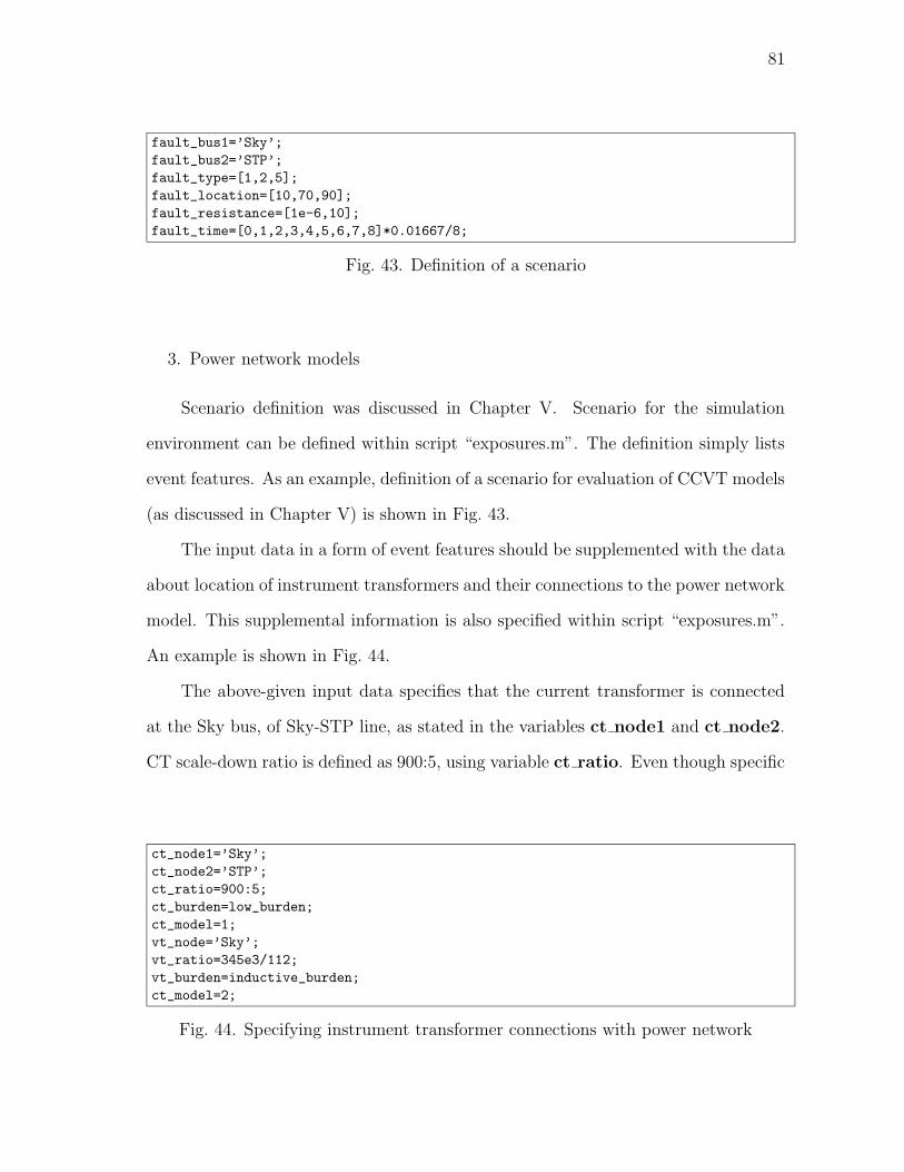
81

fault_bus1=’Sky’;

fault_bus2=’STP’;

fault_type=[1,2,5];

fault_location=[10,70,90];

fault_resistance=[1e-6,10];

fault_time=[0,1,2,3,4,5,6,7,8]*0.01667/8;

Fig. 43. Definition of a scenario

3. Power network models

Scenario definition was discussed in Chapter V. Scenario for the simulation

environment can be defined within script “exposures.m”. The definition simply lists

event features. As an example, definition of a scenario for evaluation of CCVT models

(as discussed in Chapter V) is shown in Fig. 43.

The input data in a form of event features should be supplemented with the data

about location of instrument transformers and their connections to the power network

model. This supplemental information is also specified within script “exposures.m”.

An example is shown in Fig. 44.

The above-given input data specifies that the current transformer is connected

at the Sky bus, of Sky-STP line, as stated in the variables ct node1 and ct node2.

CT scale-down ratio is defined as 900:5, using variable ct ratio. Even though specific

ct_node1=’Sky’;

ct_node2=’STP’;

ct_ratio=900:5;

ct_burden=low_burden;

ct_model=1;

vt_node=’Sky’;

vt_ratio=345e3/112;

vt_burden=inductive_burden;

ct_model=2;

Fig. 44. Specifying instrument transformer connections with power network

82

current transformer models used with the environment may have pre-set scale-down

ratio, user is still left with the freedom to manually set this ratio. The reason for

this is to allow small modifications to the ratio, usually in the limits of ±5% (e.g.

current transformer model with the ratio of 900:5 ca be used in simulations as having

the ration of (1.05 · 900 : 5). The same kind of specification are made for the CCVT,

using variables vt node and vt ratio.

Output data of exposure generators are the files containing exposure waveforms

(3 current and 3 voltage waveforms, corresponding to three phases). Waveforms are

stored in the form of Matlab matrix files. Matrix and vector variables which comprise

exposure file are:

1. Time vector t. Contains time scale produced by ATP.

2. Primary voltage signal vectors vVtnodea, vVtnodeb, vVtnodec. Mentioned

three vectors contain primary voltages, corresponding to three phases. Vtnode

is the name of the node where voltage transformer (or CCVT) is connected.

3. Secondary voltage signal vectors vVta, vVtb, vVtc. These three vectors con-

tain signals from the output of voltage transformer/CCVT models.

4. Primary current signal vectors iTerraCtsa, iTerraCtsb, iTerraCtsc. Men-

tioned three vectors contain primary current signals, from the transmission line

where current transformer is connected.

5. Secondary current signal vectors iCtnodeaCtpa, iCtnodebCtpb, iCtnodec-

Ctpc. These vectors, corresponding to three three phases, are obtained from

secondaries of current transformer model. Ctnode is the name of the node

(bus) where current transformer model is connected.

83

6. Steady-state current phasor matrix i ss. These phasors, one for each phase,

correspond to currents in the transmission line (under investigation) during

steady-state faulted condition (after transient signals die-out). First row of the

matrix contains phasor magnitudes, while second row contains phasor angles.

7. Steady-state voltage phasor matrix v ss. Explanation is the same as for matrix

variable i ss.

8. Moment of the event start t start (scalar). This is scalar value that denotes

(in [s]) when the event starts.

9. Additional information fault data, ct data, vt data. This data is simply

copied content of scenario definition and instrument transformer connection

specifications (see Figs. 43 and 44). The reason for including these fields in the

structure is to enable efficient sorting of exposure files, when storing them into

the database.

The above vectors and matrices are nested within an object structure, denoted

signals. Therefore, each of the vectors or matrices can be accessed by putting the

object structure name (followed by a period) in form of the vector or matrix name,

e.g. signals.iTerraCtsa. An example of an exposure structure is shown in Fig. 45.

Exposure files are stored (organized) in the form of database. The structure of the

exposure database, created for scenarios defined in Chapter V, is shown in Table XI.

According to the table, root directory contains every one of the main directories.

In turn, each main directory contains all the subdirectories. Prefixes “oc ” and “d ”

denote IED model A (“oc” is short for overcurrent) and IED model B (“d” is short for

distance), respectively. All the exposure files, once generated, are stored in directory

called “exposures”, corresponding to IED and instrument transformer model. Utility

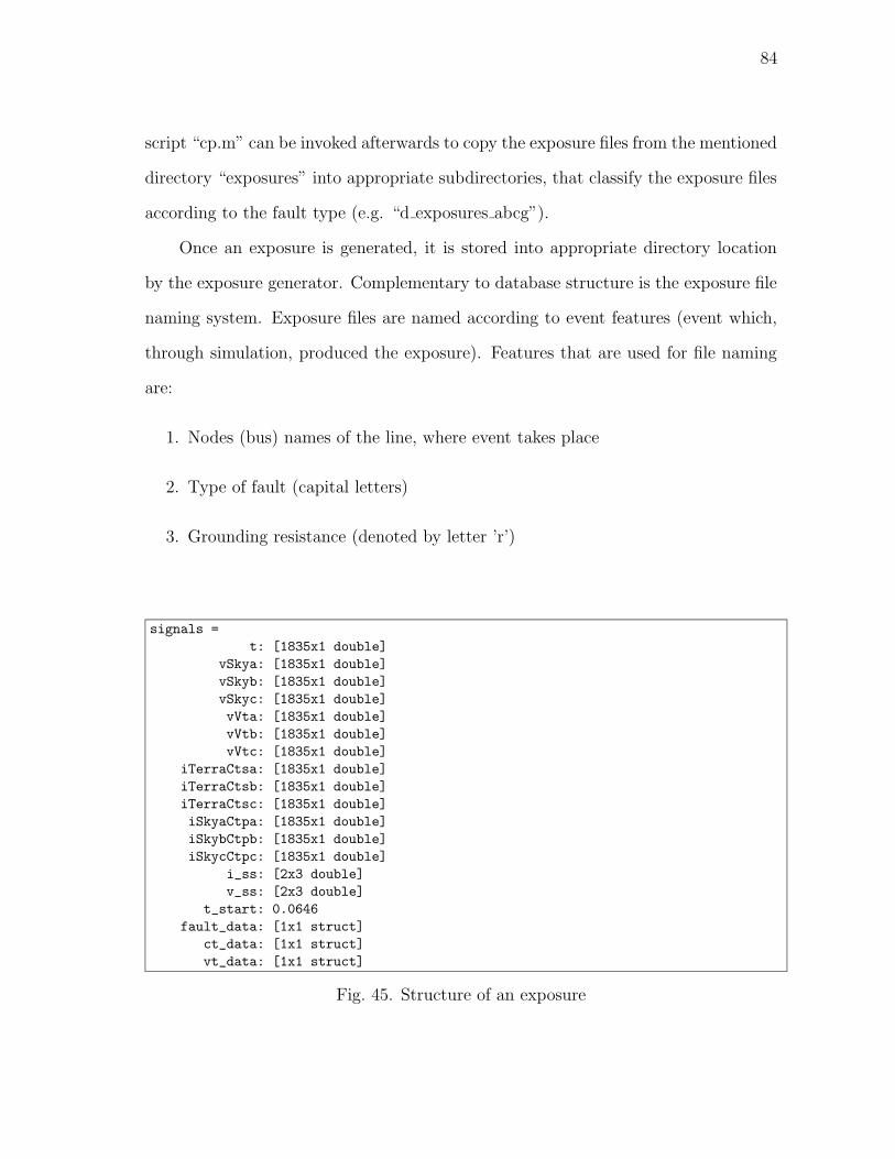
84

script “cp.m” can be invoked afterwards to copy the exposure files from the mentioned

directory “exposures” into appropriate subdirectories, that classify the exposure files

according to the fault type (e.g. “d exposures abcg”).

Once an exposure is generated, it is stored into appropriate directory location

by the exposure generator. Complementary to database structure is the exposure file

naming system. Exposure files are named according to event features (event which,

through simulation, produced the exposure). Features that are used for file naming

are:

1. Nodes (bus) names of the line, where event takes place

2. Type of fault (capital letters)

3. Grounding resistance (denoted by letter ’r’)

signals =

t: [1835x1 double]

vSkya: [1835x1 double]

vSkyb: [1835x1 double]

vSkyc: [1835x1 double]

vVta: [1835x1 double]

vVtb: [1835x1 double]

vVtc: [1835x1 double]

iTerraCtsa: [1835x1 double]

iTerraCtsb: [1835x1 double]

iTerraCtsc: [1835x1 double]

iSkyaCtpa: [1835x1 double]

iSkybCtpb: [1835x1 double]

iSkycCtpc: [1835x1 double]

i_ss: [2x3 double]

v_ss: [2x3 double]

t_start: 0.0646

fault_data: [1x1 struct]

ct_data: [1x1 struct]

vt_data: [1x1 struct]

Fig. 45. Structure of an exposure

85

Table XI. Structure of the exposures database

Root Directory Main Directories Subdirectories

results ct ref exposuresct 1 oc exposures abcgct 2 oc exposures agct 3 oc exposures bcct 4 d exposures abcgccvt 1 d exposures agccvt 2 d exposures bcccvt 3ccvt 4

4. Location of the fault along the line (denoted by letter ’l’)

5. Index number of time-point of the event (denoted by letter ’t’)

The features are included in the file name in the order as given above. All files carry

extension ’mat’, which is standard extension for Matlab matrix files. An example of

the exposure file name is “FAULT Sky Spr AG r5 l10 t4.mat”

2. Flowchart

Flowchart of the exposure generator is shown in Fig. 46. Generation of transient

waveforms (exposures), corresponding to scenario events, is carried out by invoking

ATP software. Exposure generator creates a script file based on models of power net-

work, instrument transformer models and scenario definition (input data). Flowchart

of the algorithm that performs the creation of the script is shown in Fig. 46(b). The

algorithm reads line-by-line the text file containing description of the network model.

Every line is analyzed until the line containing information about protected trans-

mission line is found. Once it is found, it is divided into two lines, by inserting a new

bus in the original line. New bus is a point on the line where events can be simulated

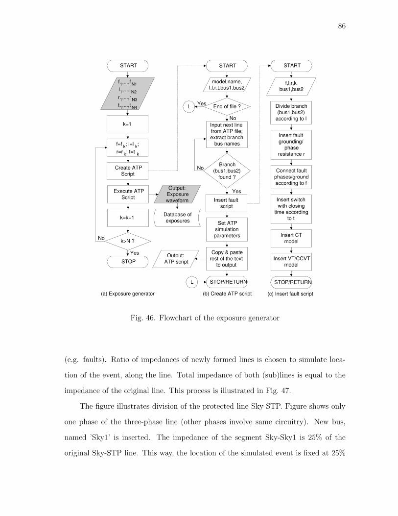
86

START

(a) Exposure generator

f 1 ,...,f N1 l 1 ,...,l N2 r 1 ,...,r N3 t 1 ,...,t N4

START

(b) Create ATP script

model name, f,l,r,t,bus1,bus2

START

Divide branch (bus1,bus2)

according to l

Insert fault grounding/

phase resistance r

f,l,r,k bus1,bus2

Connect fault phases/ground according to f

Insert switch with closing

time according to t

Insert CT model

Insert VT/CCVT model

STOP/RETURN

(c) Insert fault script

Input next line from ATP file; extract branch

bus names

Insert fault script

Yes

Set ATP simulation parameters

No Branch

(bus1,bus2) found ?

End of file ? L

Output: ATP script

Copy & paste rest of the text

to output

STOP/RETURN L

Yes

No k=1

Execute ATP Script

k=k+1

STOP

Yes

f=f k ; l=l k ; r=r k ; t=t k

Create ATP Script

No k>N ?

Output: Exposure waveform

Database of exposures

Fig. 46. Flowchart of the exposure generator

(e.g. faults). Ratio of impedances of newly formed lines is chosen to simulate loca-

tion of the event, along the line. Total impedance of both (sub)lines is equal to the

impedance of the original line. This process is illustrated in Fig. 47.

The figure illustrates division of the protected line Sky-STP. Figure shows only

one phase of the three-phase line (other phases involve same circuitry). New bus,

named ’Sky1’ is inserted. The impedance of the segment Sky-Sky1 is 25% of the

original Sky-STP line. This way, the location of the simulated event is fixed at 25%

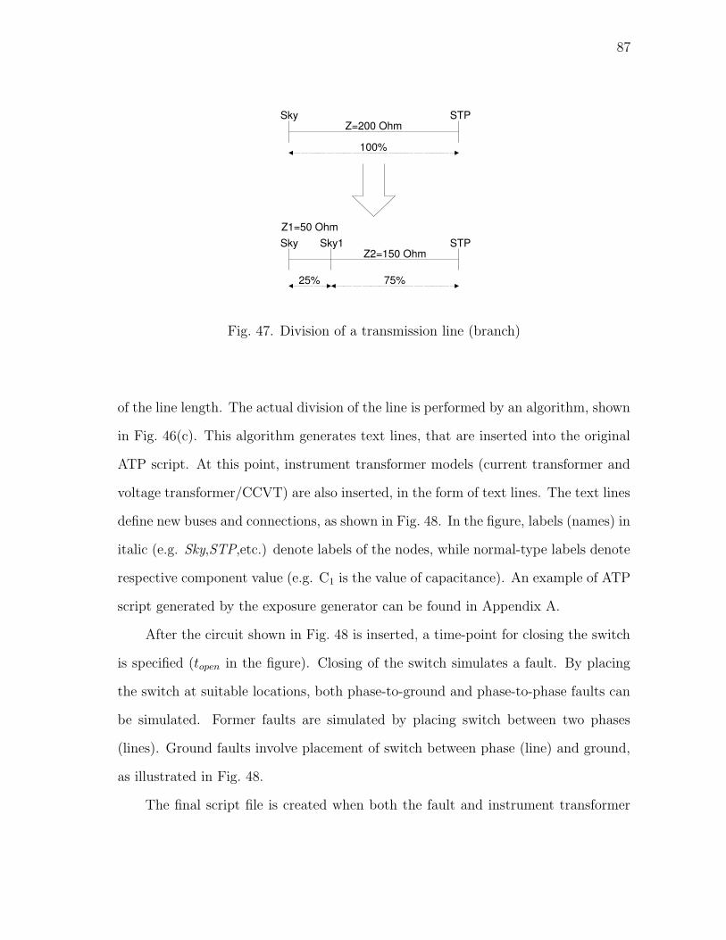
87

Sky STP

Sky STP Sky1 Z1=50 Ohm

Z2=150 Ohm

Z=200 Ohm

100%

25% 75%

Fig. 47. Division of a transmission line (branch)

of the line length. The actual division of the line is performed by an algorithm, shown

in Fig. 46(c). This algorithm generates text lines, that are inserted into the original

ATP script. At this point, instrument transformer models (current transformer and

voltage transformer/CCVT) are also inserted, in the form of text lines. The text lines

define new buses and connections, as shown in Fig. 48. In the figure, labels (names) in

italic (e.g. Sky,STP,etc.) denote labels of the nodes, while normal-type labels denote

respective component value (e.g. C1 is the value of capacitance). An example of ATP

script generated by the exposure generator can be found in Appendix A.

After the circuit shown in Fig. 48 is inserted, a time-point for closing the switch

is specified (topen in the figure). Closing of the switch simulates a fault. By placing

the switch at suitable locations, both phase-to-ground and phase-to-phase faults can

be simulated. Former faults are simulated by placing switch between two phases

(lines). Ground faults involve placement of switch between phase (line) and ground,

as illustrated in Fig. 48.

The final script file is created when both the fault and instrument transformer

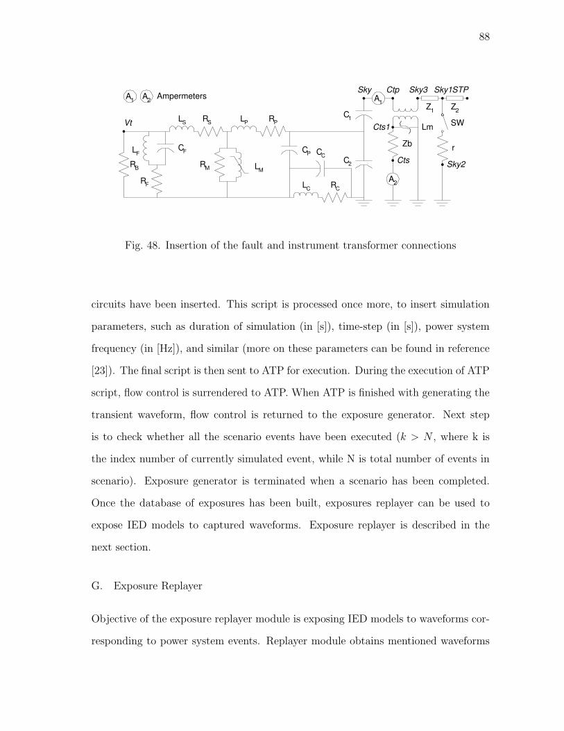
88

Vt

Sky Ctp A 1

R C L C

C C

R P L P R S L S

C F

R F

L F

R B

C 1

C 2 L M R M

C P

Zb

Lm Cts1

A 2

Sky3 STP

Z 1

Sky1

SW

r

Sky2

Z 2

Cts

A 1 A 2 Ampermeters

Fig. 48. Insertion of the fault and instrument transformer connections

circuits have been inserted. This script is processed once more, to insert simulation

parameters, such as duration of simulation (in [s]), time-step (in [s]), power system

frequency (in [Hz]), and similar (more on these parameters can be found in reference

[23]). The final script is then sent to ATP for execution. During the execution of ATP

script, flow control is surrendered to ATP. When ATP is finished with generating the

transient waveform, flow control is returned to the exposure generator. Next step

is to check whether all the scenario events have been executed (k > N , where k is

the index number of currently simulated event, while N is total number of events in

scenario). Exposure generator is terminated when a scenario has been completed.

Once the database of exposures has been built, exposures replayer can be used to

expose IED models to captured waveforms. Exposure replayer is described in the

next section.

G. Exposure Replayer

Objective of the exposure replayer module is exposing IED models to waveforms cor-

responding to power system events. Replayer module obtains mentioned waveforms

89

from the database of exposures, generated by exposure generator. Other sources can

also be used, such as custom-built database of field-recorded data.


Input of the module consists of:

1. Pointer to database of exposures

2. Pointer to IED models

First pointer is variable root (global variable), which value specifies root direc-

tory location of the exposure database (see Table XI). Second pointer is the file name

of the Simulink model of IED (this point will be discussed in more detail in the text

to follow).

Output of exposure replayer are files containing IED model response signals. As

before, files are stored as Matlab matrix files, with standard extension “mat”. In the

case of IED model A, mentioned signals are recorded at two points:

1. Output of measuring element

2. Output of decision making element

In the case of IED model B, signals are recorded only at output of decision making

element.

File naming system used in the exposure replayer is similar as in the exposure

generator. The only difference is in the file name prefix. Measuring element output

is stored in the file named starting with “OC M” (“M” is short for measuring), while

decision making element output is stored in files starting with “OC D” and “D D”

(“D” is short for decision making).

90

Measuring file contains two object structures, called i and v. Both structure

contains the same variables. In the case of structure i mentioned variables contain

signals from current-measurement element, while in the case of v, the signals are from

voltage-measurement element. The variables are:

1. Steady-state phasor matrix ss. The meaning of this variable is the same as in

the case of exposure generator (see previous section).

2. Measured phasor magnitude and phase vectors a amp, a ph, b amp, b ph,

c amp, c ph. These vectors contains signals measured by the Fourier algorithm

measuring element.

3. Original exposure waveform vectors a, b, c. Vectors containing copies of original

waveforms (that are sent to the input of measuring element), corresponding to

three phases, are included for use by statistical analyzer, which will be discussed

in the next section.

4. Time vector t and moment of the event start t start (scalar). Meaning is

similar to the exposure generator (see previous section). There is difference,

however: the time scale, contained in vector t is generated by Simulink, which

may be (and usually is) different than the one generated by ATP. ATP generates

time scale with equally spaced time-points, while Simulink, depending on the

chosen solving method, may produce time scale where time-steps are not equal.

Decision making file contains two vector and one scalar variable. The variables

are:

1. Time vector t and moment of the event start t start (scalar). Meaning is the

same as in the case of the measuring file.

91

2. Trip signal vector trip. This vectors contains trip signal derived by decision

making element.

Mentioned measuring and decision making files are stored (organized) in the form

of database. The structure of the response database, created for scenarios defined

in Chapter V, is shown in Table XII. This database has the same structure as

the database of exposures (see Table XI). The content of the response database

is complementary to content of exposure database. Together, the two databases

form one, general database. This database can also be used outside the simulation

environment.

2. Flow Chart

Flowchart of the exposure generator is shown in Fig. 49(a). Replayer performs a

loop, in which exposures are sequentially read from the database, and replayed. The

loop is performed until the database has been exhausted (k > N , where k is the

index number of currently replayed exposure, while N is total number of exposures

in database). Actions performed to replay an exposure are:

1. Set variables i in and v in to contain exposure. The content of these vari-

ables is sent directly to IED model using Simulink. The Matlab code that

performs this is shown in Fig. 50. In the code, variable s contains exposure (see

Fig. 45), while variable ref flag determines what instrument transformer is be-

ing evaluated (referent instrument transformer, current transformer or voltage

transformer/CCVT). Variables i in and v in are a communication channel be-

tween simulation environment and Simulink. This communication is shown in

Fig. 51. Different IED models can be incorporated into simulation environment

by observing structure of variables i in, v in.

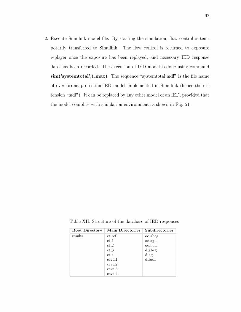
92

2. Execute Simulink model file. By starting the simulation, flow control is tem-

porarily transferred to Simulink. The flow control is returned to exposure

replayer once the exposure has been replayed, and necessary IED response

data has been recorded. The execution of IED model is done using command

sim(’systemtotal’,t max). The sequence “systemtotal.mdl” is the file name

of overcurrent protection IED model implemented in Simulink (hence the ex-

tension “mdl”). It can be replaced by any other model of an IED, provided that

the model complies with simulation environment as shown in Fig. 51.

Table XII. Structure of the database of IED responses

Root Directory Main Directories Subdirectories

results ct ref oc abcgct 1 oc agct 2 oc bcct 3 d abcgct 4 d agccvt 1 d bcccvt 2ccvt 3ccvt 4

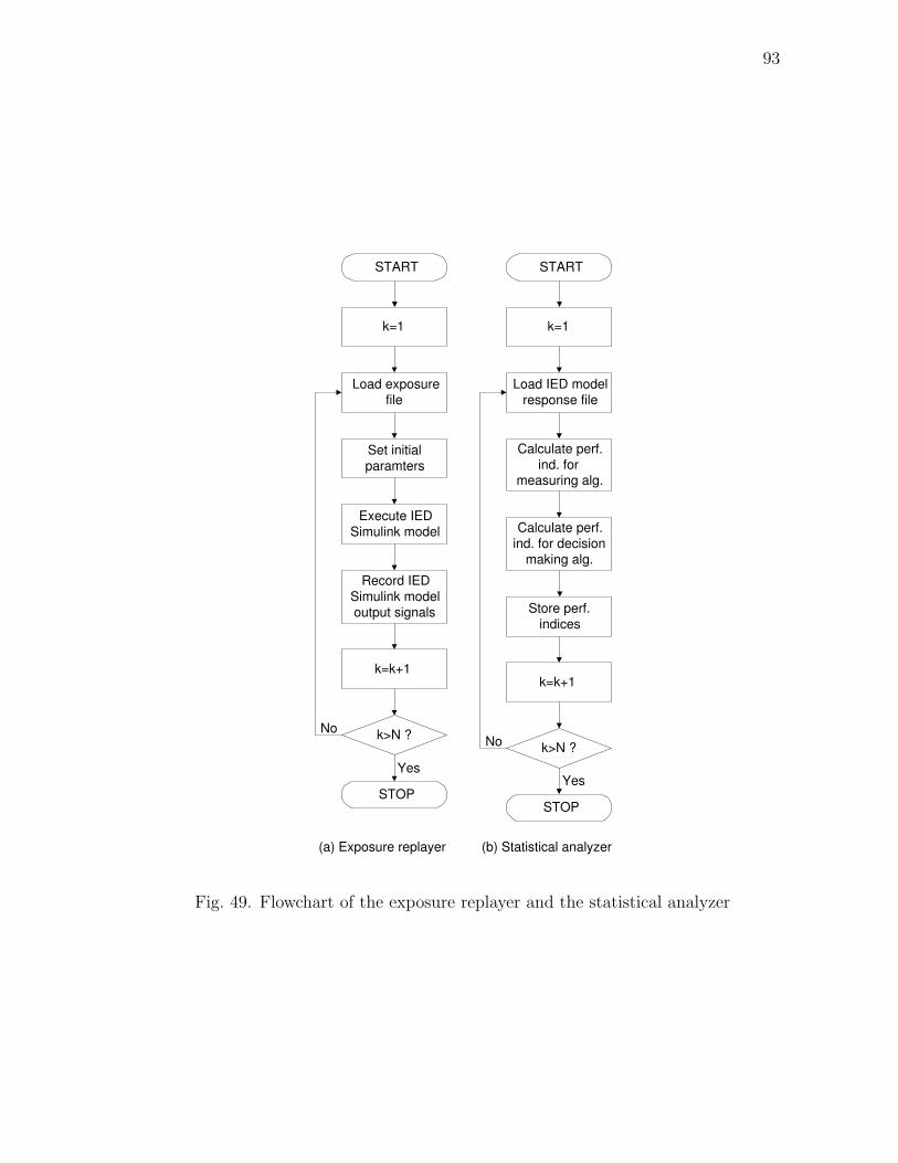
93

START START

Load IED model response file

Calculate perf. ind. for

measuring alg.

k=1

Calculate perf. ind. for decision

making alg.

(a) Exposure replayer (b) Statistical analyzer

No No

STOP

k>N ?

k=k+1

Yes

Store perf. indices

Load exposure file

Set initial paramters

Execute IED Simulink model

k=1

Record IED Simulink model output signals

STOP

k>N ?

k=k+1

Yes

Fig. 49. Flowchart of the exposure replayer and the statistical analyzer

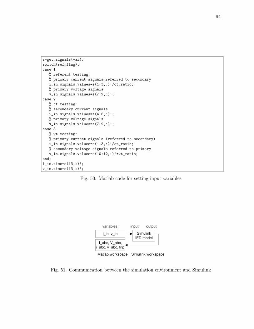
94

s=get_signals(var);

switch(ref_flag);

case 1

% referent testing:

% primary current signals referred to secondary

i_in.signals.values=s(1:3,:)’/ct_ratio;

% primary voltage signals

v_in.signals.values=s(7:9,:)’;

case 2

% ct testing:

% secondary current signals

i_in.signals.values=s(4:6,:)’;

% primary voltage signals

v_in.signals.values=s(7:9,:)’;

case 3

% vt testing:

% primary current signals (referred to secondary)

i_in.signals.values=s(1:3,:)’/ct_ratio;

% secondary voltage signals referred to primary

v_in.signals.values=s(10:12,:)’*vt_ratio;

end;

i_in.time=s(13,:)’;

v_in.time=s(13,:)’;

Fig. 50. Matlab code for setting input variables

i_in, v_in

I_abc, V_abc, i_abc, v_abc, trip

Simulink IED model

input output

Matlab workspace

variables:

Simulink workspace

Fig. 51. Communication between the simulation environment and Simulink

95

H. Statistical Analyzer

Objective of the statistical analyzer is derivation of numerical values of performance

indices, defined in Chapter IV. The calculation is carried out as described in Chap-

ter IV.


Input of the statistical analyzer is a pointer to top of the database of responses (path

to root directory). This pointer is specified using variable root (global variable).

Output of statistical analyzer are files, containing performance indices. Files are

stored as Matlab matrix files, carrying extension “mat”. In case of IED model A,

the indices are calculated for both measuring and decision making elements, while in

case of model B, indices are calculated only for decision making element.

File naming convention used in the statistical analyzer is simple: file name prefix

for IED model A is “OCDATA ”, and for model B the prefix is “DDATA ”. The prefix

is followed by the instrument transformer model, which was used in simulations for

derivation of particular indices (stored in the file). Prefix is followed by the name of

instrument transformer model. An example of a file containing performance indices

is “OCDATA ct 1.mat”. Mentioned files are stored according to the structure of the

response database, shown in Table XII. One file, containing performance indices, is

stored in each of subdirectories.

Performance indices file contains two structures: m and d. The first one con-

tains performance indices for measuring element, while the second structure contains

indices for decision making element. First structure is present only in the case of IED

model A indices.

Structure m has two sub-structures: i and v. First sub-structure contains indices

96

for current measuring element, while second sub-structure contains indices for voltage

measuring element. The variables contained in sub-structures are:

1. Gain for the DC component dc gain a, dc gain b, dc gain c.

2. Aggregated index F F a, F b, F c.

3. Settling time s a, s b, s c.

4. Overshoot o a, o b, o c.

5. Normalized error index, e a, e b, e c.

Structure d has two scalar variables:

1. Time-point of the start of event scalar t start.

2. Time-point of issuing a trip signal t trip. In the case of IED model B this

variable is not scalar, but a two-element vector, where first element denotes trip

time for zone 1, and second element denotes trip time for zone 2.

Performance indices file contains a sequence of sets of indices. Sets from one file

correspond to a subdirectory of a database of IED response. Subdirectories within

the structure of this database is where performance indices files are stored.

2. Data Formatter

Additional utility scripts, data formatters called “oc average” and “d average”, can

be used for finding average values of performance indices. Average values are found

by analyzing every file of performance indices and simply calculating the mean value

of all the indices store in that particular files. Mentioned utility modules also have

the ability of generating output data in form of tables. Tables can exported as:

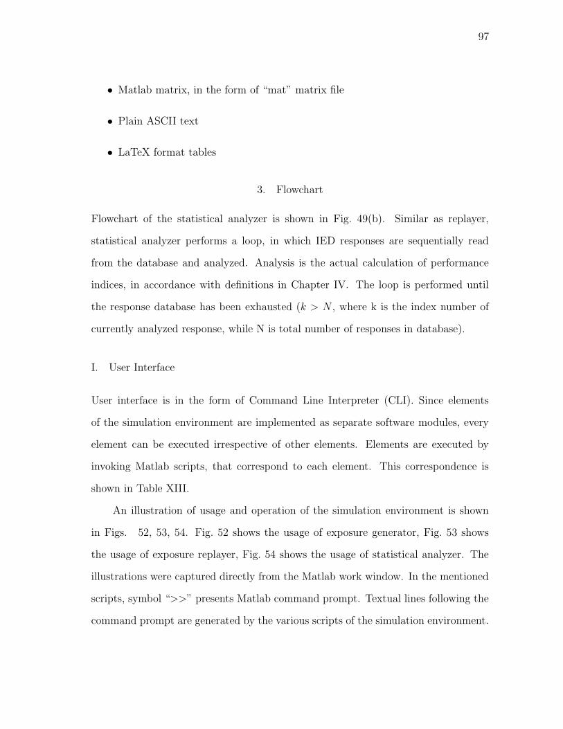
97

• Matlab matrix, in the form of “mat” matrix file

• Plain ASCII text

• LaTeX format tables

3. Flowchart

Flowchart of the statistical analyzer is shown in Fig. 49(b). Similar as replayer,

statistical analyzer performs a loop, in which IED responses are sequentially read

from the database and analyzed. Analysis is the actual calculation of performance

indices, in accordance with definitions in Chapter IV. The loop is performed until

the response database has been exhausted (k > N , where k is the index number of

currently analyzed response, while N is total number of responses in database).

I. User Interface

User interface is in the form of Command Line Interpreter (CLI). Since elements

of the simulation environment are implemented as separate software modules, every

element can be executed irrespective of other elements. Elements are executed by

invoking Matlab scripts, that correspond to each element. This correspondence is

shown in Table XIII.

An illustration of usage and operation of the simulation environment is shown

in Figs. 52, 53, 54. Fig. 52 shows the usage of exposure generator, Fig. 53 shows

the usage of exposure replayer, Fig. 54 shows the usage of statistical analyzer. The

illustrations were captured directly from the Matlab work window. In the mentioned

scripts, symbol “>>” presents Matlab command prompt. Textual lines following the

command prompt are generated by the various scripts of the simulation environment.

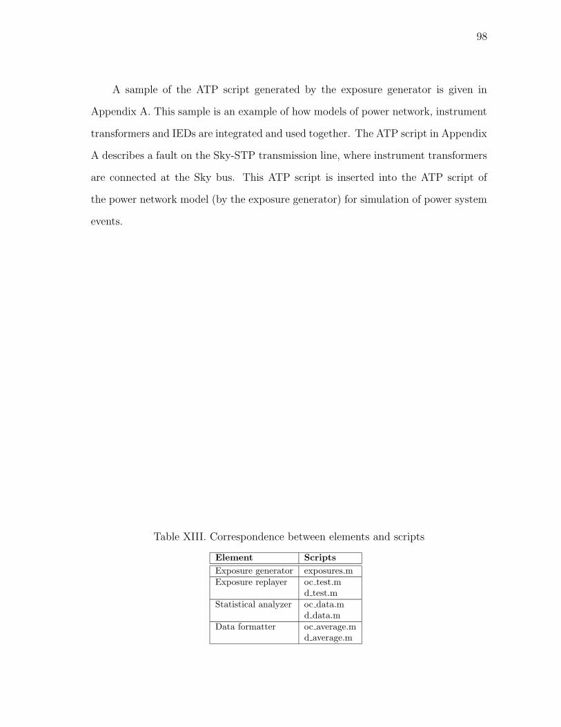
98

A sample of the ATP script generated by the exposure generator is given in

Appendix A. This sample is an example of how models of power network, instrument

transformers and IEDs are integrated and used together. The ATP script in Appendix

A describes a fault on the Sky-STP transmission line, where instrument transformers

are connected at the Sky bus. This ATP script is inserted into the ATP script of

the power network model (by the exposure generator) for simulation of power system

events.

Table XIII. Correspondence between elements and scripts

Element Scripts

Exposure generator exposures.mExposure replayer oc test.m

d test.mStatistical analyzer oc data.m

d data.mData formatter oc average.m

d average.m

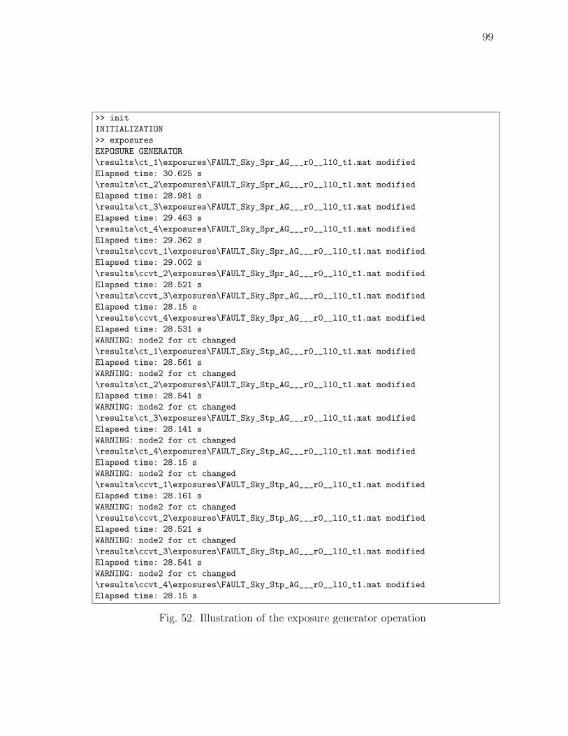
99

>> init

INITIALIZATION

>> exposures

EXPOSURE GENERATOR

\results\ct_1\exposures\FAULT_Sky_Spr_AG___r0__l10_t1.mat modified

Elapsed time: 30.625 s







\results\ccvt_1\exposures\FAULT_Sky_Spr_AG___r0__l10_t1.mat modified








WARNING: node2 for ct changed

\results\ct_1\exposures\FAULT_Sky_Stp_AG___r0__l10_t1.mat modified












\results\ccvt_1\exposures\FAULT_Sky_Stp_AG___r0__l10_t1.mat modified











Fig. 52. Illustration of the exposure generator operation

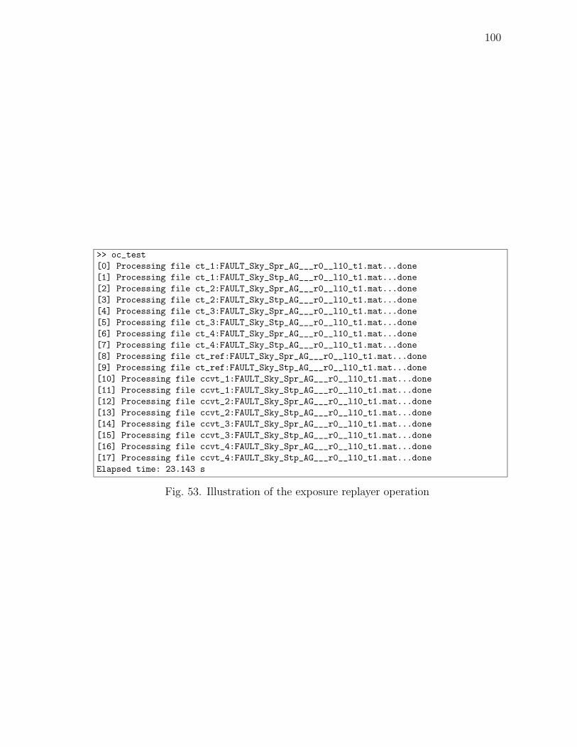
100

>> oc_test

[0] Processing file ct_1:FAULT_Sky_Spr_AG___r0__l10_t1.mat...done

[1] Processing file ct_1:FAULT_Sky_Stp_AG___r0__l10_t1.mat...done







[8] Processing file ct_ref:FAULT_Sky_Spr_AG___r0__l10_t1.mat...done

[9] Processing file ct_ref:FAULT_Sky_Stp_AG___r0__l10_t1.mat...done

[10] Processing file ccvt_1:FAULT_Sky_Spr_AG___r0__l10_t1.mat...done

[11] Processing file ccvt_1:FAULT_Sky_Stp_AG___r0__l10_t1.mat...done








Fig. 53. Illustration of the exposure replayer operation

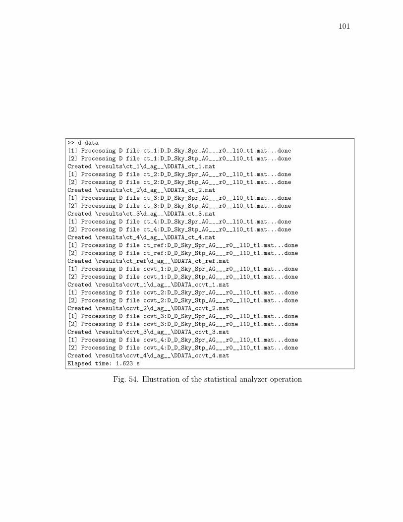
101

>> d_data

[1] Processing D file ct_1:D_D_Sky_Spr_AG___r0__l10_t1.mat...done

[2] Processing D file ct_1:D_D_Sky_Stp_AG___r0__l10_t1.mat...done

Created \results\ct_1\d_ag__\DDATA_ct_1.mat










[1] Processing D file ct_ref:D_D_Sky_Spr_AG___r0__l10_t1.mat...done

[2] Processing D file ct_ref:D_D_Sky_Stp_AG___r0__l10_t1.mat...done

Created \results\ct_ref\d_ag__\DDATA_ct_ref.mat

[1] Processing D file ccvt_1:D_D_Sky_Spr_AG___r0__l10_t1.mat...done

[2] Processing D file ccvt_1:D_D_Sky_Stp_AG___r0__l10_t1.mat...done

Created \results\ccvt_1\d_ag__\DDATA_ccvt_1.mat











Fig. 54. Illustration of the statistical analyzer operation

102

J. Integration of Different Models

Simulation environment can be used with different power network, instrument trans-

former and IED models. The recommendations for use of different models is as

follows:

• Power network model is defined by ATP script, that contains description of

the network. The location of the mentioned ATP script is defined in variable

power network model (global variable) in script “init.m”. Different power

network models can be created as standard ATP scripts. ATP scripts should

be stored within “models” directory of the root directory.

• Instrument transformers are defined by Matlab scripts “ct model.m” and “vt model.m”.

Different instrument transformer models can be created using the template

stored in the mentioned Matlab scripts. Additional files (such as files “HYST.PCH”,

which define hysteresis curves) should be stored in “models” directory of the

root directory.

• IED models are defined by Simulink models. Location of these models can be

specified using Matlab and Simulink search path setting (see reference [33] for

specific instructions). Names of IED Simulink models are specified in scripts

“overcurrent.m” and “distance.m”. Different IED models can be defined by

specifying their names in the two mentioned script files. Different models

must follow the communication channels (between simulation environment and

Simulink) specified in Fig. 51. It is also important to store IED models response

in the following variables:

– i in, v in contain input current and voltage signals (from exposures, see

Fig. 45)

103

– i abc, v abc, I abc, V abc receive output signals from the measuring

element (see Chapter V)

– trip receives output from the decision making element (see Chapter V)

K. Conclusion

Simulation environment and its software implementation were described in this chap-

ter. Simulation environment is a practical contribution of this thesis. It is imple-

mented in form of software modules. One of the goals of the simulation environment

is its expendability. This means that software was developed in such a way, that

user can modify or add software modules, according to his/her research objectives.

Special attention was paid to explanation of I/O data structure and flowchart of the

environment. Three major elements of the environment are: 1) exposure generator,

2) exposure replayer and 3) statistical analyzer. Implementation of the elements was

described and discussed first. Afterwards, user interface was explained. Together,

major elements and user interface form a comprehensive software package.

Conclusion is that simulation environment can be used for extensive research

in the area of instrument transformer evaluation. Simulation environment offers

seamless interaction between several software packages, such as ATP, Matlab and

Simulink. This interaction enables incorporation of wide variety of models of instru-

ment transformers and IEDs. Possible applications of the simulation environment,

beside evaluation of influence of instrument transformers, include evaluation of instru-

ment transformer response, comparison of different instrument transformer designs,

etc.

104

CHAPTER VII

EVALUATION METHODOLOGY APPLICATION AND RESULTS

A. Introduction

This chapter presents application of the evaluation methodology. Results are obtained

by using simulation environment described in the previous chapter. As described in

Chapter VI, final results present average values of performance indices. Average

values were calculated according to the structure of the databases, as explained in

Chapter VI.

B. Impact on the IED Model A

IED model A has outputs available at both measuring element (current and voltage)

and decision making element (see section C of Chapter V). Therefore, influence of

instrument transformers on both elements was evaluated. Evaluation criteria is listed

and explained in Chapter IV. The results are presented in the following sections.

1. Interpretation of Performance Indices for the Measurement Element

In order to interpret the values of performance indices for the measurement element, it

is necessary to define what values of the indices are indication of expected (“good”)

performance, and what values are indication of unexpected (“bad”) performance.

Generally, the lower the value, the better (more expected) the performance. How-

ever, since it is unrealistic to expect zero values, the following values can be used as

indication of acceptable performance:

• Settling time (t2%) should be less than eight signal periods, i.e. 0.133 s

• Overshoot (∆y%) should be less than 10 %

105

• Absolute value of normalized error index (|∆e%|) should be less than 5 %

• Gain for DC component (FRDC) should be less than 30 %

• Aggregated index (F ) should be less than 0.01

The chosen values simply reflect the preferences of the author. Selection of the

above mentioned values follows the practice defined in reference [16]. The values are

also based around typical average of the performance indices of the referent instrument

transformer.

2. Measurement Element Performance Indices

Values of performance indices for current measurement element of IED model A are

shown in Tables XIV through XVI. Values for voltage measurement element are

shown in Tables XVII through XIX.

Table XIV. Current measuring element, ABCG fault

Model t2% ∆y% ∆e% FRDC F

Referent 0.126 0.082 0.019 0.283 0.004CT 1 0.126 0.079 0.070 0.175 0.005CT 2 0.126 0.015 0.551 0.036 0.006CT 3 0.126 0.100 0.054 0.215 0.005CT 4 0.126 0.047 0.164 0.073 0.005

Table XV. Current measuring element, AG fault



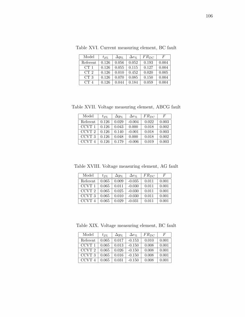
106

Table XVI. Current measuring element, BC fault



Table XVII. Voltage measuring element, ABCG fault


Referent 0.126 0.029 -0.004 0.022 0.003CCVT 1 0.126 0.043 0.000 0.018 0.002CCVT 2 0.126 0.140 -0.001 0.018 0.003CCVT 3 0.126 0.048 0.000 0.018 0.002CCVT 4 0.126 0.179 -0.006 0.019 0.003

Table XVIII. Voltage measuring element, AG fault


Referent 0.065 0.009 -0.035 0.011 0.001CCVT 1 0.065 0.011 -0.030 0.011 0.001CCVT 2 0.065 0.025 -0.030 0.011 0.001CCVT 3 0.065 0.010 -0.030 0.011 0.001CCVT 4 0.065 0.029 -0.031 0.011 0.001

Table XIX. Voltage measuring element, BC fault


Referent 0.065 0.017 -0.153 0.010 0.001CCVT 1 0.065 0.013 -0.150 0.008 0.001CCVT 2 0.065 0.026 -0.150 0.008 0.001CCVT 3 0.065 0.016 -0.150 0.008 0.001CCVT 4 0.065 0.031 -0.150 0.008 0.001

107

The following conclusions can be made, based on performance indices of the

current measuring element:

• Influence of instrument transformer models on the settling time is relatively

negligible (or small).

• Influence of instrument transformer models on overshoot varies significantly.

Smallest overshoot is caused by current transformer model 2. Overshoot caused

by this model is several times lower than the one caused by the referent instru-

ment transformer. Significant decrease in overshoot indicates current trans-

former saturation, as discussed in Chapter IV. Current transformer model 4

shows slightly larger overshoot than model 2, while the rest of models caused

overshoot levels close to what is found in the referent one.

• Influence on normalized error index also varies significantly. As in the case of

overshoot, current transformer model 2 caused largest error, in the range from

30 % to 56 %. This error range is significant, and indicates possible misoperation

by IED. Current transformer model 4 caused an increased error, at the level of

16 %, while the rest of the models did not cause the error to increase above 7

%.

• Influence on DC gain showed that current transformer model 2 suppresses DC

component better than the rest of the models. Since it was already concluded

that current transformer model 2 underwent saturation in significant number of

test cases, it can be concluded that saturation actually enhances suppression of

DC component. Current transformer model 4 also showed good DC suppression,

compared to the rest of the models.

• Influence of instrument transformer models on aggregated frequency index is

108

negligible .

The following conclusions can be made, based on performance indices of voltage

measuring element:

• CCVT models do not influence the settling time.

• CCVT models 2 and 4 caused significantly higher overshoot than for the referent

one (overshoot is at least two times higher). The reason for this is the nature

of the burden connected to model 2 and 4: inductive. Other models did cause

slightly increased overshoot, than the referent model.

• The influence of instrument transformer models is relatively negligible (or small)

on normalized error index. The same holds true for the influence on DC gain

and aggregated frequency index.

3. Decision Making Element Performance Indices

Values of performance indices for decision making element of IED model A are shown

in Tables XX through XXII. Note: mentioned performance indices for decision mak-

ing element need a further clarification. Basis criteria is defined in Chapter IV.

Meaning of indices in Tables XX through XXII is:

• N1 is number of correct trip assertions for faults in forward direction of protec-

tion

• F1 is number of incorrect trip restrains for faults in forward direction

• N2 is number of correct trip restrains for faults in backward direction

• F2 is number of incorrect trip assertions for faults in backward direction

109

• s1 is defined as:

s1 =N1

Nforward

(7.1)


s2 =N2

Nbackward

(7.2)

where Nforward = 48 is number of faults simulated in forward zone of protection, and

Nbackward = 16 is number of faults simulated in backward zone. Ideal IED performance

would produce N1 = 48 and N2 = 16. The rest of performance indices are listed and

defined in Chapter IV.

The following conclusions can be made, based on the results:

• Current transformer model 2 caused the poorest performance of IED model.

Detection of ABCG faults is impacted the most, while AG and BC faults are

detected slightly better. The influence of current transformer model 2 is de-

grading IED model performance to unacceptable levels in the case of all three

faults.

• Current transformer models, other than current transformer model 2, showed

no influence on decision making element of IED model A. Current transformer

model 4 did lower selectivity of IED model in backward zone slightly.

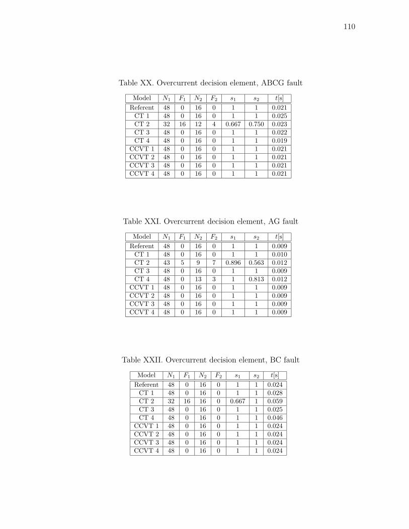
110

Table XX. Overcurrent decision element, ABCG fault

Model N1 F1 N2 F2 s1 s2 t[s]

Referent 48 0 16 0 1 1 0.021CT 1 48 0 16 0 1 1 0.025CT 2 32 16 12 4 0.667 0.750 0.023CT 3 48 0 16 0 1 1 0.022CT 4 48 0 16 0 1 1 0.019

CCVT 1 48 0 16 0 1 1 0.021CCVT 2 48 0 16 0 1 1 0.021CCVT 3 48 0 16 0 1 1 0.021CCVT 4 48 0 16 0 1 1 0.021

Table XXI. Overcurrent decision element, AG fault


Referent 48 0 16 0 1 1 0.009CT 1 48 0 16 0 1 1 0.010CT 2 43 5 9 7 0.896 0.563 0.012CT 3 48 0 16 0 1 1 0.009CT 4 48 0 13 3 1 0.813 0.012


Table XXII. Overcurrent decision element, BC fault


Referent 48 0 16 0 1 1 0.024CT 1 48 0 16 0 1 1 0.028CT 2 32 16 16 0 0.667 1 0.059CT 3 48 0 16 0 1 1 0.025CT 4 48 0 16 0 1 1 0.046


111

C. Impact on the IED Model B

IED model B has output available only for decision making elements. Values of

performance indices for decision making element of IED model B are shown in Tables

XXIII through XXV. Meaning of indices in Tables XX through XXII, based on

criteria defined in Chapter IV, is:

• N1 is number of correct trip assertions for faults in primary zone of protection

• F1 is number of trip assertions with incorrect time-delay, for faults in primary

zone of protection (faults detected as belonging to backup zone)

• N2 is number of correct trip assertions for faults in backup zone of protection

• F2 is number of trip assertions with incorrect time-delay, for faults in backup

zone of protection (faults detected as belonging to primary zone)


s1 =N1

Nprimary

(7.3)


s2 =N2

Nbackup

(7.4)

where Nprimary = 32 is number of faults simulated in primary zone of protection, and

Nbackup = 32 is number of faults simulated in backup zone. Ideal IED performance

would produce N1 = 32 and N2 = 32. Indices t1 and t2 are average tripping times for

faults in primary and backup zones, respectively (average tripping time is calculated

only for correct trip assertions). In cases where t2 could not be calculated because

of IED model misoperation (e.g. none of the faults in zone 2 were recognized), an

asterisk (*) was placed in the Table entries (corresponding to the mentioned cases).

The following conclusions can be made, based on the results:

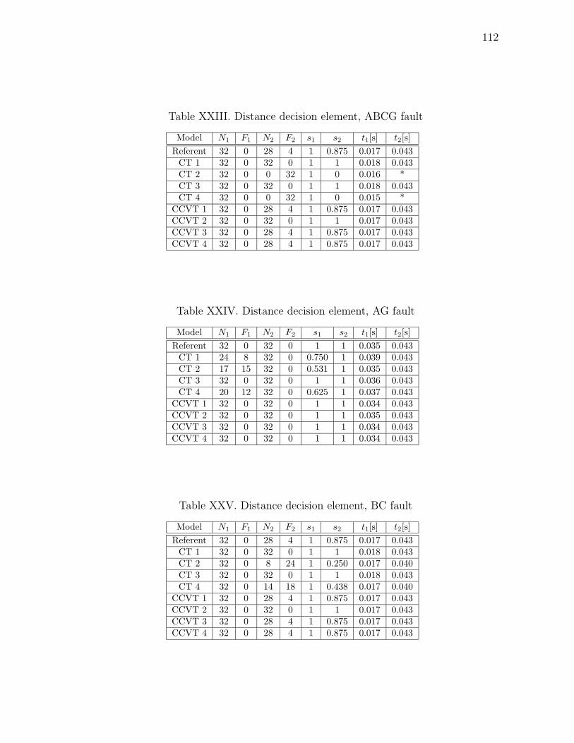
112

Table XXIII. Distance decision element, ABCG fault

Model N1 F1 N2 F2 s1 s2 t1[s] t2[s]

Referent 32 0 28 4 1 0.875 0.017 0.043CT 1 32 0 32 0 1 1 0.018 0.043CT 2 32 0 0 32 1 0 0.016 *CT 3 32 0 32 0 1 1 0.018 0.043CT 4 32 0 0 32 1 0 0.015 *

CCVT 1 32 0 28 4 1 0.875 0.017 0.043CCVT 2 32 0 32 0 1 1 0.017 0.043CCVT 3 32 0 28 4 1 0.875 0.017 0.043CCVT 4 32 0 28 4 1 0.875 0.017 0.043

Table XXIV. Distance decision element, AG fault


Referent 32 0 32 0 1 1 0.035 0.043CT 1 24 8 32 0 0.750 1 0.039 0.043CT 2 17 15 32 0 0.531 1 0.035 0.043CT 3 32 0 32 0 1 1 0.036 0.043CT 4 20 12 32 0 0.625 1 0.037 0.043

CCVT 1 32 0 32 0 1 1 0.034 0.043CCVT 2 32 0 32 0 1 1 0.035 0.043CCVT 3 32 0 32 0 1 1 0.034 0.043CCVT 4 32 0 32 0 1 1 0.034 0.043

Table XXV. Distance decision element, BC fault


Referent 32 0 28 4 1 0.875 0.017 0.043CT 1 32 0 32 0 1 1 0.018 0.043CT 2 32 0 8 24 1 0.250 0.017 0.040CT 3 32 0 32 0 1 1 0.018 0.043CT 4 32 0 14 18 1 0.438 0.017 0.040

CCVT 1 32 0 28 4 1 0.875 0.017 0.043CCVT 2 32 0 32 0 1 1 0.017 0.043CCVT 3 32 0 28 4 1 0.875 0.017 0.043CCVT 4 32 0 28 4 1 0.875 0.017 0.043

113

• From performance of IED model B connected to referent instrument transform-

ers, it can be seen that IED model shows small overreach for ABCG and BC

fault types (selectivity in zone 2 is 87.5 %). However, IED model B showed no

overreach effects when connected to current transformer models 1 and 3, and

CCVT model 2. It can be concluded that mentioned instrument transformer

models have positive influence on IED model B. However, this positive influence

of mentioned instrument transformer models does not remove IED model’s in-

herent internal problem of overreach. If the IED model B had not been tested

using the referent model, the inherent overreach would not be discovered. Men-

tioned instrument transformer models masked (hid) the overreach.

• Current transformer models 2 and 4 caused IED model to overreach complete

zone 2 for ABCG fault type. The reason for this is larger error in measurement,

cause by mentioned current transformer models.

D. Conclusion

This chapter presented results from application of the evaluation methodology. Re-

sults were obtained using the simulation environment. Methodology is described in

Chapter V, while simulation environment is presented in Chapter VI. Results confirm

existing observation about influence of instrument transformers of IED performance.

Results also point-out to some new aspects of this influence, which have not been

presented in literature so far.

Observations that can be made, based on results from the application of method-

ology, are:

• Influence of various instrument transformer models differs significantly. In gen-

eral, CCVT models (which include models of voltage transformers) have sig-

114

nificantly smaller impact on IED model performance. This indicates that in

practice, voltage transforming devices (voltage transformers and CCVTs) are

expected to cause IED misoperations in extremely small number of cases. It can

be hard to even detect these influences using field-recorded data. Simulation

environment is, therefore, a useful tool in analyzing situations when corrupting

influence of CCVTs is suspected.

• Influence of current transformer models varies significantly from one model to

another. Main cause of differences are model parameters. In general, burden

magnitude and VI characteristic of electromagnetic core are two major sources

of corruptive instrument transformer influence. This is confirmed by the results.

• Saturation, phenomena associated with current transformers, actually enhances

certain aspects of current transformer response. Results have shown that, for

example, measuring algorithm suppresses the DC offset better for input signals

supplied from a saturated current transformer. Simulation environment is a

useful tool in further researching of this effect.

• Distortions in IED input signals may lead to a better IED performance, com-

pared to performance of IED supplied with undistorted input signals. Even

though this may seem as a desired influence of instrument transformers, it is

not. Bad performance (such as overreaching, which was demonstrated in the

results) can be masked, i.e. not detected, when connected to current transform-

ers that cause signal distortions. This is an important observation for transient

testing of IEDs. Simulation environment can be used as supplement to existing

testing tools to investigate transient response of the protective relays in more

detail, regarding the mentioned hiding (masking).

115

Conclusion is that results, delivered by simulation environment, are comprehen-

sive and meaningful. It was presented how various instrument transformer aspects

influence elements of IEDs, and how this influence shapes the performance of IEDs.

Therefore, simulation environment was shown, through application, to be a useful

and novel tool for analysis of the influence of instrument transformers on protective

IED performance.

116

CHAPTER VIII

CONCLUSION

A. Summary

Instrument transformers (IT) are crucial components of power protection system.

Their objective is to supply scaled-down replicas of power network current and voltage

signals. Depending on accuracy of these replicas, faulty conditions are recognized

and properly and timely dealt with by protection system. This, in turn, affects the

operation of power system.

Conventional instrument transformer are based on electromagnetic coupling be-

tween power network on the primary side, and protective devices on the secondary

side. Side-effect of this coupling are signal distortions. Protective devices and other

IEDs are sensitive to these distortions. This sensitivity can lead to misoperation,

which consequently, may lead to disruption of power system operation.

A way of overcoming this problem is introducing novel, optical instrument trans-

formers, called transducers. The improvement, made possible by the new current

and voltage sensing technology, is enabling distortion-free replicas of signals from

the primary side of transducers. However, these improvements are still barely tested

through field application experiences.

There is still an uncertainty about whether the new technology is superior to the

conventional one. This uncertainty is summarized by questions:

1. What is the difference in performance between the conventional instrument

transformers and novel, optical transducers ?

2. How can this difference be practically measured or evaluated ?

Existing approaches to solving the problem, available in the literature, do not

117

offer systematic and comprehensive answers to these questions. On the other hand,

the answer is necessary to asses benefits of the new technology. This thesis pro-

poses a new methodology for evaluation of influence of instrument transformers on

IED performance. Existing approaches focus mostly on evaluation of either instru-

ment transformer response, or IED performance. Difference between methodology

presented in this thesis and existing ones, is that the proposed methodology is com-

bining mentioned approaches into unique a procedure. This procedure can lead to

answers to the mentioned questions.

While developing and applying the methodology, several steps were taken. Steps

are described in various chapters of this thesis. First, instrument transformer per-

formance characteristics were analyzed in Chapter II. It was shown that instrument

transformer performance characteristics are the root of distortions. Various instru-

ment transformer designs were discussed. Three performance characteristics were

identified as having the major impact on generation of distortions: accuracy, fre-

quency bandwidth and transient response. Impact of mentioned characteristics on

distortions was described. It was concluded that distortions can be significant.

Sensitivity of protective devices to distortions was addressed in Chapter III. It

was shown that protective devices do not show degradation in performance when ex-

posed to signal distorted up to a certain threshold level. However, distortion levels

above the threshold cause IEDs to miss-operate. Miss-operation includes unaccept-

ably high increase of operationing time and/or unacceptably low selectivity. It was

concluded that distortions caused by conventional instrument transformers can lead

to IED misoperation.

Criteria and new methodology for evaluation of the influence of instrument trans-

formers was presented in Chapter IV. Criteria was defined for measuring and decision

making elements of protective IEDs. Some problems, when calculating numerical val-

118

ues for the criteria, and how to overcome the problems were also addressed. The new

methodology covered important aspects of evaluation: 1) why is evaluation impor-

tant, 2) what are the means for quantifying the influence (finding numerical values), 3)

what is the best procedure for finding the quantitative values of the influence, 4) what

is the meaning of the quantitative values. It was concluded that new methodology

presents systematic and comprehensive approach to the problem solution.

Simulation approach to evaluation was described in Chapter V. Main aspects

of simulation, models and scenarios, were discussed. First, simulation procedure was

discussed. Power network, instrument transformer and IED models were presented,

along with reasoning for the choice. Simulation scenarios were presented next. It was

concluded that, by proper choice of models and proper scenario definitions, meaningful

results can be obtained through simulation.

Simulation environment, which presents software implementation of the method-

ology, was presented in Chapter VI. The environment enables seamless interaction be-

tween several software packages. The environment is implemented in form of software

modules. Three main modules, exposure generator, exposure replayer and statistical

analyzer, were described in detail. Particular importance was placed on description of

I/O data structure and flowchart. These aspects are important for the users who wish

to modify or expand the environment. It was concluded that environment presents a

useful tool for application of the methodology.

Application of evaluation methodology was presented in Chapter VII. Results

obtained through simulation were presented. Results both confirmed existing observa-

tions and offered some new insights, considering influence of instrument transformers

on protective IEDs. New insights include: certain distortions (such as the one caused

by saturation) can be detected by analyzing numerical values of performance indices,

instrument transformers can mask (hide) bad IED performance. It was concluded

119

that simulation environment can be used for obtaining meaningful and comprehen-

sive results.

Thesis contributions are both theoretical and practical. Both contributions are

summarized in the next section.

B. Contribution

At present, there is no comprehensive and systematic methodology for evaluation of

the influence of instrument transformers on protective IEDs. The main contribution

of this thesis is a new methodology for evaluation.

Theoretical contributions of the thesis are:

• Connection between instrument transformer characteristics, signal distortions

and IED sensitivity was established (Chapters II and III). It was shown that

instrument transformer characteristic have direct impact on IED performance,

and therefore may affect power system operation.

• Criteria and methodology for evaluation of the influence of instrument trans-

formers was defined (Chapter IV). Criteria was defined in form of numerical

performance indices. Methodology was defined through steps for the evaluation

procedure.

Practical contributions of the thesis are:

• Modelling and simulation approach to evaluation of influence of instrument

transformers was established (Chapter V). It was shown how to choose models

in order to achieve meaningful results through simulation.

• Simulation environment was developed (Chapter VI). Environment is in the

form of software modules. Environment was shown to be a useful tool in ana-

120

lyzing influence of instrument transformers. Other benefits of the environment

include its modifiability and expendability.

• Methodology was applied through simulations, using developed simulation en-

vironment (Chapter VII). It was shown that this approach can successfully

provide information about influence of instrument transformer characteristics

on IED performance. The results can be used for further research.

121

REFERENCES

[1] P. M. Anderson, Power System Protection, New York, NY: McGraw-Hill, 1999,

p. 23-34.

[2] J. L. Blackburn, Protective Relaying: Principles and Applications, New York,

NY: Marcel Dekker, 1998, p. 26-28, 129-141, 151-157.

[3] C. Christos, A. Wright, Electrical Power System Protection, Boston, MA: Kluwer

Academic Publishers, 1999, p. 39-103.

[4] Power Systems Communication Committee, Working Group Fiber Optics Sen-

sors of the Fiber Optics Subcommittee, “Optical current transducers for power

systems: A review,” IEEE Transactions on Power Delivery, vol. 9, no. 4, pp.

1778-1788, October 1994.

[5] Power Systems Relaying Committee, Working Group of the Relay Input Sources

Subcommittee, “Transient response of current transformers,” IEEE Transactions

on Power Apparatus and Systems, vol. 96, no. 6, pp. 1809-1814, November 1977.

[6] Power Systems Relaying Committee, Working Group of the Relay Input Sources

Subcommittee, “Transient response of coupling capacitor voltage transformers,”

IEEE Transactions on Power Apparatus and Systems, vol. 100, no. 12, pp. 4811-

4814, December 1981.

[7] M.I. Samesima, J.C. de Oliveira, E.M. Dias, “Frequency response analysis and

modeling of measurement transformers under distorted current and voltage sup-

ply,” IEEE Transactions on Power Delivery, vol. 6, no. 4, pp. 1762-1768, October

1991.

122

[8] M. Kezunovic, C. Fromen, F. Phillips, Lj. Kojovic, A. Abur, D. Sevcik, “Ex-

perimental evaluation of EMTP based current transformer models for protective

relay transient study,” IEEE Transactions on Power Delivery, vol. 9, no. 1, pp.

405-413, January 1994.

[9] D. Tziouvaras, P. McLaren, C. Alexander, D. Dawson, J. Esztergalyos,

C. Fromen, M. Glinkowski, I. Hasenwinkle, M. Kezunovic, L. Kojovic, B.

Kotheimer, R. Ruffel, J. Nordstrom, S. Zochol, “Mathematical models for cur-

rent, voltage and coupling capacitor voltage transformers,” IEEE Transactions

on Power Delivery, vol. 15, no. 1, pp. 62-72, January 2000

[10] M. Kezunovic, A. Abur, Lj. Kojovic, V. Skendzic, H. Singh, “DYNA-TEST

simulator for relay testing, Part II: Performance evaluation,” IEEE Transactions

on Power Delivery, vol. 7, no. 3, pp. 1097-1103, July 1992.

[11] J.R. Lucas, P.G. McLaren, W.W.L. Keerthipala, R.P. Jayasinghe, “Improved

simulation models for current and voltage transformers in relay studies,” IEEE

Transactions on Power Delivery, vol. 7, no. 1, pp. 152-159, January 1992.

[12] P.G. McLaren, R.P. Jayasinghe, “Simulation of CTs operating in parallel in a

differential current protection scheme,” in Proceedings of IEEE Communications,

Power and Computing Conference, vol. 1, no. 1, Winnipeg, MB, Canada, May

1997, pp. 126-131.

[13] M. Kezunovic, J.T. Cain, B. Perunicic, S. Kreso, “Digital protective relaying

algorithm sensitivity study and evaluation,” IEEE Transactions on Power De-

livery, vol. 3, no. 3, pp. 912-922, July 1988.

[14] E. A. Udren, J. A. Zipp, “Proposed statistical performance measures for

microprocessor-based transmission-line protective relays, Part I: Explanation of

123

the statistics,” IEEE Transactions on Power Delivery, vol. 12, no. 1, pp. 134-143,

January 1997.

[15] E. A. Udren, J. A. Zipp, “Proposed statistical performance measures for

microprocessor-based transmission-line protective relays, Part II: Collection and

uses of data,” IEEE Transactions on Power Delivery, vol. 12, no. 1, pp. 144-156,

January 1997.

[16] M. Kezunovic, B. Kasztenny, “Design optimization and performance evaluation

of the relay algorithms, relays and protective systems using advanced testing

tools,” IEEE Transactions on Power Delivery, vol. 15, no. 4, pp. 1129-1135,

October 2000.

[17] M.S. Sachdev, T.S. Sidhu, P.G. McLaren, “Issues and opportunities for testing

numerical relays,” in Proceedings of IEEE Power Engineering Society Summer

Meeting, vol. 2, no. 1, New York, NY, May 1997, pp. 1185-1190.

[18] M. Kezunovic, Q. Chen, “A novel approach for interactive protection system

simulation,” IEEE Transactions on Power Delivery, vol. 12, no. 2, pp. 668-674,

April 1997.

[19] M. Kezunovic, Y.Q. Xia, Y. Guo, C.W. Fromen, D.R. Sevcik, “Distance relay

application testing using a digital simulator,” IEEE Transactions on Power De-

livery, vol. 12, no. 1, pp. 72-82, January 1997.

[20] M. Kezunovic, Y.Q. Xia, Y. Guo, C.W. Fromen, D.R. Sevcik, “An advanced

method for testing of distance relay operating characteristic,” IEEE Transactions

on Power Delivery, vol. 11, no. 1, pp. 149-157, January 1996.

[21] M. Kezunovic, A. Abur, Lj. Kojovic, V. Skendzic, H. Singh, “DYNA-TEST

124

simulator for relay testing, Part I: Design characteristics,” IEEE Transactions

on Power Delivery, vol. 6, no. 4, pp. 1423-1429, October 1991.

[22] IEEE Standard C57.13-1993, Requirements for Instrument Transformers, IEEE,

New York, NY, June 1993, pp. 1-73.

[23] CanAm EMTP User Group, Alternative Transient Program (ATP) Rule Book,

Portland, OR, January 1992.

[24] Lj. Kojovic, M. Kezunovic, S.L. Nilsson, “Computer simulation of a ferrores-

onance suppression circuit for digital modeling of coupling capacitor voltage

transformers,” in Proceedings of ISMM Conference on Computer Applications

in Design, Simulation and Analysis, vol. 1, no. 1, Orlando, FL, March 1992, pp.

20-24.

[25] R. C. Dugan, M. F. McGranaghan, H. W. Beaty, Electrical Power Systems Qual-

ity, New York, NY: McGraw-Hill, 1996, p. 1-38.

[26] Lj. A. Kojovic, “Impact of current transformer saturation on overcurrent pro-

tection operation,” in Proceedings of IEEE Power Engineering Society Summer

Meeting, vol. 3, no. 1, New York, NY, July 2002, pp. 1078-1083.

[27] M.A. Hughes, “Distance relay performance as affected by capacitor voltage trans-

formers,” Proceedings of IEE, vol. 121, no. 12, pp. 1557-1566, December 1974.

[28] W.D. Humpage, K.P. Wong, “Influence of capacitor-voltage-transfomers on the

dynamic response of distance protection,” Electrical Engineering Transactions,

vol. 14, no. 2, pp. 59-63, June 1978.

[29] M. Kezunovic, A. Abur, G. Huang, “MERIT 2000 - A new concept in power en-

gineering education,” in Proceedings of Energy Management and Power Delivery

125

Conference, vol. 1, no. 1, Singapore, March 1998, pp. 54-59.

[30] H.O. Pascual, J.A. Rapallini, “Behaviour of Fourier, cosine and sine filtering

algorithms for distance protection, under severe saturation of the current mag-

netic transformer,” in Proceedings of IEEE Power Tech Conference, vol. 4, no.

1, Porto, Portugal, September 2001, pp. 6-12.

[31] D. Ristanovic, S. Vasilic, M. Kezunovic, “Design and implementation of scenarios

for evaluating and testing distance relays,” in Proceedings of 33rd North American

Power Symposium, vol. 1, no. 1, College Station, TX, October 2001, pp. 470-475.

[32] IEEE Standard C37.112-1996, Inverse-Time Characteristic Equations for Over-

current Relays, IEEE, New York, NY, January, 1996, pp. 1-13.

[33] The MathWorks, Inc., Using MATLAB, Natick, MA, January 1999.

[34] The MathWorks, Inc., Using Simulink, Natick, MA, June 1990.

[35] The MathWorks, Inc., Power System Blockset Users Guide, Natick, MA, January

1999.

126

APPENDIX A

C ** FAULT DATA START **

/BRANCH

C ** CT MODEL CONNECTION DATA START **

-1SKY3A SKY1A .435942.00994.3725150.69 0 0 0

-2SKY3B SKY1B .06143 .56647.6245150.69 0 0 0

-3SKY3C SKY1C 0

C ** CT MODEL START **

/BRANCH

CTS1A CTSA 8.33 .175 0

/BRANCH

CTS1B CTSB 8.33 .175 0

/BRANCH

CTS1C CTSC 8.33 .175 0

/BRANCH

96 CTS1A 0.0 0.0 0

$INCLUDE, C:\ATP37\atp2\models\HYST_2.pch

96 CTS1B 0.0 0.0 0


96 CTS1C 0.0 0.0 0


/SOURCE

14CTS1A 1E-10 60. -1. 10.

18 180.SKY3A CTPA

14CTS1B 1E-10 60. -1. 10.

18 180.SKY3B CTPB

14CTS1C 1E-10 60. -1. 10.

18 180.SKY3C CTPC

/SWITCH

CTSA MEASURING 1

CTSB MEASURING 1

CTSC MEASURING 1

SKYA CTPA MEASURING 1

SKYB CTPB MEASURING 1

SKYC CTPC MEASURING 1

C ** CT MODEL END **

C == CCVT MODEL START ==

/BRANCH

N2A N3A 228. 0

N1A SKYA .82938 0

N1A 32.497 0

N1A N2A 21997. 0

N1A N3A .03770 0

N3A 5.7E-8 0

127

TRANSFORMER TA0001 5.E5 0

9999

1N3A 400. 1131. 8.586

2VTA .2 .377 .112

N5A VTA 3600. 0

N5A VTA 263.89 0

N5A 37.5 0

VTA 100. 0

N2B N3B 228. 0

N1B SKYB .82938 0

N1B 32.497 0

N1B N2B 21997. 0

N1B N3B .03770 0

N3B 5.7E-8 0

TRANSFORMER TB0001 5.E5 0

9999

1N3B 400. 1131. 8.586

2VTB .2 .377 .112

N5B VTB 3600. 0

N5B VTB 263.89 0

N5B 37.5 0

VTB 100. 0

N2C N3C 228. 0

N1C SKYC .82938 0

N1C 32.497 0

N1C N2C 21997. 0

N1C N3C .03770 0

N3C 5.7E-8 0

TRANSFORMER TC0001 5.E5 0

9999

1N3C 400. 1131. 8.586

2VTC .2 .377 .112

N5C VTC 3600. 0

N5C VTC 263.89 0

N5C 37.5 0

VTC 100. 0

/OUTPUT

SKYA SKYB SKYC VTA VTB VTC

C == CCVT MODEL END ==

/BRANCH

C ** CT MODEL CONNECTION DATA END **

-1SKY1A STPA .435942.00994.372516.744 0 0 0

-2SKY1B STPB .06143 .56647.624516.744 0 0 0

-3SKY1C STPC 0

/SWITCH

SKY1A SKY1B .064583 10. 0

/BRANCH

/SWITCH

SKY1B SKY1C .064583 10. 0

/BRANCH

/SWITCH

128

SKY1A SKY2A .064583 10. 0

/BRANCH

/BRANCH

SKY2A 5. 0

C ** FAULT DATA END **

129

VITA

Bogdan Naodovic was born in 1977 in Novi Sad, Yugoslavia. He received his

Bachelor of Science degree in electrical engineering (Diploma of Engineering) from

the Faculty of Technical Sciences, University of Novi Sad, Yugoslavia, on December

29, 2001. In undergraduate studies, he majored in telecommunications.

Bogdan Naodovic entered graduate school at Texas A&M University in the Sum-

mer of 2002. His emphasis in graduate school was in the area of power systems and

instrument transformers. During his graduate studies, he worked on various research

assignments as a research assistant. He was also Power System Control and Protection

Lab manager.

Author’s address:

Texas A&M University

Department of Electrical Engineering

College Station, Texas 77843-3128

influence of instrument transformers on · pdf fileali abur (member) krishna r. narayanan...

Documents