HAL Id: hal-00414849https://hal.archives-ouvertes.fr/hal-00414849

Submitted on 26 Jun 2013

HAL is a multi-disciplinary open accessarchive for the deposit and dissemination of sci-entific research documents, whether they are pub-lished or not. The documents may come fromteaching and research institutions in France orabroad, or from public or private research centers.

L’archive ouverte pluridisciplinaire HAL, estdestinée au dépôt et à la diffusion de documentsscientifiques de niveau recherche, publiés ou non,émanant des établissements d’enseignement et derecherche français ou étrangers, des laboratoirespublics ou privés.

Influence of structural variability upon soundperception : Usefulness of fractional factorial designs

Vincent Koehl, Etienne Parizet

To cite this version:Vincent Koehl, Etienne Parizet. Influence of structural variability upon sound perception : Use-fulness of fractional factorial designs. Applied Acoustics, Elsevier, 2006, 67 (3), pp.249-270.�10.1016/j.apacoust.2005.06.002�. �hal-00414849�

Influence of structural variability upon sound

perception: usefulness of fractional factorial

designs

Vincent Koehl ∗, Etienne ParizetLaboratoire Vibrations Acoustique, Institut National des Sciences Appliquees,

F-69621 Villeurbanne Cedex, France

Abstract

The present paper introduces an efficient and time-saving approach for the evalu-ation of the consequences of structural uncertainties on sound perception. Its aimis to validate the use of fractional factorial designs for perceptual assessment ofa model system. A test bench was used, which allowed to accurately control thevariability of several structural design parameters. Sounds emitted by the benchwere recorded with a dummy head and submitted to listeners during two experi-ments, in which they had to evaluate the dissimilarity of each sound to a reference,representing the nominal state of the device. In the first experiment, six factors,assumed to be independent, were used to define a fractional factorial design. As ananalysis of variance showed that two interactions between factors should have beentaken into account, a second experimental design was developed to quantify theseinteractions. These two experiments allowed to define an accurate model of soundperception, describing the effect of each factor on the perceived dissimilarity. Thusit was possible to relate the variability of the structure to the perception of thesound emitted with few experimental effort.

Key words: Structural uncertainties; Sound Perception; Fractional factorialdesigns; Taguchi tables; Listening test; Dissimilarity

1 Introduction

Because of mechanical variability affecting its structure, an object resultingfrom an industrial production can exhibit considerable variability in its vi-bratory and acoustical behavior [1-4]. For instance, Bernhard and Kompella[1] showed that, on a large panel of cars, the frequency response functionsdue to air-borne and structure-borne excitations could exhibit non-negligible

∗ Corresponding author. Tel:+33-4-72-43-70-37; fax:+33-4-72-43-87-12.Email address: vkoehl@lva.insa-lyon.fr (Vincent Koehl).

Preprint submitted to Applied Acoustics 8 July 2005

amplitude fluctuations and resonance frequencies shifts. The general problemis to determine whether structural dispersions may also give rise to percep-tual dispersions. In other words, can the perception of the sound emitted byan object be significantly modified by variability affecting its structure? Eventhough consequences of uncertainties on the radiated sound have been stud-ied [3,4] and can be objectively predicted, it is not yet possible to link theconsequences of these uncertainties to the perceptual aspect. The aim of thispaper is to present a tool to evaluate the acoustical outcomes of structuraluncertainties on sound perception.

It might be assumed that the knowledge of Just Noticeable Differences (JNDs)should allow to predict that influence. JNDs are the perceptual thresholdsabove which a listener can perceive a variation of a sound feature. However,though the loudness’ JNDs are well known (see [5] for a review on the topic),this is not the case for some other psychoacoustic metrics such as roughnessand fluctuation strength. Moreover, it is not possible to predict the soundfeatures that will be used by listeners to evaluate differences between complexsounds. The knowledge of JNDs alone does not provide information aboutthe type of indicators that are used to differentiate stimuli. But they providecomplementary information about the possible relevancy of the psychoacousticmetrics used by listeners for the differentiation task.

Therefore, the only way of measuring a small perceptual difference betweencomplex sounds is an adequate listening test. In order to obtain statisticallysignificant results, studies about structural uncertainties generally involve alarge number of recordings. As an example, in [1], the sample group was com-posed of ninety-nine cars. For a perceptual study, such a large number ofsounds is far too high. To evaluate the influence of relevant variability param-eters with a reasonable number of sounds, efficient fractional factorial designscan be used. In such experimental designs, which are often used in many in-dustrial applications [6,7], several factors are varied simultaneously accordingto a special experimental layout. The goal is to use a systematic approach forexperimentation such that each experiment provides relevant information.

Fractional factorial designs have been used in a lot of studies aiming to im-prove processes and to spare measurement time [8,9]. However, their mainapplication is the field of physical measurement. Up to now, published studiesusing fractional factorial designs for perceptual purposes involved a few num-ber of factors [10] and disregarded any possible interaction. In [11], fractionalfactorial designs have been used to correlate the sound quality of a vacuumcleaner to the spectral content of sounds. If the presence of significant interac-tions is presumed, full factorial designs are preferred [12]. Fractional factorialdesigns have not yet been used so far to evaluate the consequences of struc-tural uncertainties on sound perception, which was the main purpose of thisstudy.

2

If this approach, which has already shown its efficiency for the understand-ing of objective vibro-acoustic data , proves to be reliable for the analysis ofsubjective data, it enables to spare much measurement and testing time.

The goal here was to introduce a model of subjective dissimilarity and to builda reliable predictive tool with fractional factorial designs.

2 Experimental setup for sound recordings

The listening test stimuli were sounds emitted by a device on which severalstructural variability parameters could be controlled.

2.1 Apparatus and experimental design

The test bench in this study was an electric machine on which dispersions,caused by typical variability of rotating machines, were simulated. Six vari-ability parameters, considered as relevant ones, were selected initially:

• ’axial misalignment’ (A) and ’angular misalignment’ (C): misalignmentswere applied to the elastic coupling by acting on the bearings that supportthe drive shaft.

• ’distance between gears’ (B): the distance was measured and adjusted.• ’outer ring inclination’ (D): the ring inclination was forced on the bearing

shown on the diagram.• ’dynamic unbalance’ (E): unbalancing masses were mounted on a flywheel

attached to the drive shaft.• ’magnetic brake torque’ (F ): fluctuations of the magnetic brake torque were

caused by modulating the feed current.

According to the fractional factorial designs terminology, these variability pa-rameters were the design factors. These factors were chosen because of theireasily recognizable spectral signature [13]. Moreover, they could be preciselycontrolled on the test bench. Three levels were assigned to each factor tocharacterize their influence. Table 1 summarizes the factors chosen and theirlevels.

Level 1 of each factor is its nominal state, levels 2 and 3 are typical valuesof misplacement caused by uncertainties. These variability parameters havebeen distributed all along the kinematic chain, as shown in Fig. 1.

3

The number of possible factors combinations is 729 (36). Hence a full factorialdesign for this case would have required too many measurements and toomuch testing time, the listener’s task being by far too difficult. Therefore,a fractional factorial design was chosen. Among fractional designs, the mostcommonly used have been defined by Taguchi and Konishi [14]. According toTaguchi tables, an orthogonal design was chosen to quantify the effects of eachfactor with a low number of measurements. Here orthogonal means that eachfactor level is equally combined with other factor levels. Assuming that therewas no interaction between factors, the experiment table referenced as L18 in[15], needing only 18 measurements, was used.

Table 2 shows the combinations of factor levels for each measurement. Fouradditional measurements were added to the L18 design to check the validity ofthe model resulting from the results of the experimental design. The measure-ment referenced as S1-1 corresponded to the reference condition of the bench,in which each factor was at its nominal level.

2.2 Measurement procedure

First, for each measurement, the test bench was set to the configuration in-dicated by the corresponding line of Table 2. Each of the six factors was setto the level defined by the measurement number. Once the test bench wasadjusted, its radiated noise was digitally recorded (fs=44100 Hz, 16-bits res-olution) using an acoustic dummy head (Bruel & Kjær type 4100) equippedwith two free-field microphones (Bruel & Kjær type 4189). All recording de-vices were located approximately 1.5 m distant from the test bench (see Fig.2). To be used as stimuli for the listening test, these recorded sounds werelimited to 3 s and submitted to a short fade in and fade out to avoid clicks.

3 First listening test: determination of main effects

3.1 Subjects

Subjects were students and members of the laboratory. They were eight womenand twenty-two men, aged from 22 to 61 (average age=31, standard devia-tion=10). Eight of them had already taken part in listening tests. All subjectsreported normal hearing.

4

3.2 Test procedure

Sounds were presented for binaural hearing (using a set of Sennheiser HD600headphones) at their original level, ranging from 75.6 to 85.5 dBA. Listenerswere asked to evaluate the dissimilarity between each test sound (S1-i) andthe reference one (n◦S1-1 in Table 2). Pretests were done in using pairedcomparisons, the reference sound being randomly presented either in first orsecond place. Subjects could listen to a pair of sounds as often as they wantedto. Thereafter they had to assess the dissimilarity of the sound pair on acontinuous scale running from ”identical” (”identique”) to ”very different”(”tres different”). Instructions for listeners were displayed on the screen beforethe test start. A necessary condition for using fractional factorial designs isthat the answer is measured on a continuous scale. This experiment did notgive evaluable results, as sounds were assessed to be either very close or verydifferent from the reference. Such dichotomic answers could not be regardedas continuous.To allow the listeners to refine their ratings, a mixed method (see Fig. 3),i.e. a combination between absolute rating and comparison, was chosen then.This test procedure was adapted from a method used for the evaluation ofpleasantness [18]. All sounds (the reference, eighteen sounds from the designand four validation ones) were presented on the test window at the same time,randomly ordered (the arbitrary number attributed to each sound in the testwindow had no link with its number in Table 2). Sounds were rated by listenerson a continuous scale running from ”identical to the reference” (”identique a lareference”, dissimilarity mark 0) to ”very different from the reference” (”tresdifferent de la reference”, dissimilarity mark 1), the rating resolution (less thanone hundredth of the full scale) being almost continuous. Again instructionsfor listeners were displayed on the screen before the test start. Subjects couldlisten to each sound as often as they wanted to in order to give answers. Tomake their task easier and allow them to give finely graded answers, they weregiven the possibility of reorganizing sounds from the closest to the furthestdistance from the reference. The test duration varied from 12 min to 21 minand was typically 16 min.

3.3 Data analysis

3.3.1 Dissimilarity ratings

Fig. 4 shows the mean dissimilarity marks, averaged over all subjects, in their95% confidence interval, for the 22 sounds. The lower the dissimilarity scoreis, the more the sound had been perceived as close to the reference. Sound S1-1, according to Table 2, was the reference. It was almost unanimously rated

5

0. The narrow 95% confidence interval excluded the hypothesis of differentlyanswering subsets within the listeners panel and confirmed that the analysisof the experimental design could be carried out with the mean scores.

3.3.2 Test reliability

To check the test reliability, two listeners did the test twice, after an interval onone week. The test-retest comparison on a same subject clearly showed similaranswers, as an example is shown on Fig. 5. The difference between the twoseries of answers was small, indicating a very good reliability. The Pearson’scorrelation coefficient r for the test-retest answers of the two listeners wasrespectively 0.906** and and 0.911** (p<.01).

3.3.3 Continuity of the answer

As shown in Fig. 6, small differences in the listeners’ judgment behavior couldbe deduced from their answers.

Some of them answered in a way that was close to a ranking of sounds, themost representative case being shown in Fig. 6(a). The two extreme soundswere rated 0 and 1, the other ones being equally spaced between these twolimits. On the other hand, as shown in Fig. 6(b), several listeners seemed to dothe task in a different way and gave equal marks to the sounds they perceivedas equally dissimilar to the reference.

Most listeners gave answers within these two schematic behaviors. Hence itwas assumed that answers fulfilled the requirement to be given on a continuousscale and they were averaged over the panel. No normalization of individualanswers was done before averaging, for two reasons:

• Most subjects made use of the full available scale, rating sounds from 0 to1.

• Inter-individual differences could be due to different answering strategies,but also to differences in the way sounds were perceived, which should notbe compensated.

3.3.4 Factor effects

To investigate the effect of the factors described in subsection 2.1 on the dis-similarity scores, an analysis of variance was carried out. The relevancy andcontribution of each factor are shown in Table 3. Some factors had obviouslymuch more influence than others. The factor ’distance between gears’ (B) con-tributed to more than 50% of the total variance, while a non-negligible part

6

(about 20%) remained unexplained. On the other hand, ’angular misalign-ment’ (C) and ’dynamic unbalance’ (E) showed a very weak contribution tothe observed variances of the answers.

A more detailed analysis should show the effect of the specific factor levels onthe judgment. Averaging the scores of all configurations having in commonone factor at a given level, the difference with the overall average was theeffect of the considered factor level on the measured response. For instancethe effect of factor ’axial misalignment’ (A) at level 1 EA1 on the measuredresponse is given by:

EA1 =MS1−1 + MS1−2 + MS1−3 + MS1−10 + MS1−11 + MS1−12

6− MS1 (1)

where MS1−i is the mean dissimilarity score (i.e. the distance to the reference)for sound n◦S1-i. All 6 MS1−j on the fraction line of Eq. (1) have in commonthat the corresponding sounds are emitted from configurations where the fac-tor A is at the level 1 (j = 1, 2, 3, 10, 11, 12 according to Table 2). MS1 is the

mean of dissimilarity judgments (MS1 =∑

18

i=1MS1−i

18= 0.52).

The effects of all factors at all levels are summarized in Table 4. The strongesteffect (+0.301) is observed for factor ’distance between gears’ (B) at level 2and the weakest (-0.003) for factor ’angular misalignment’ (C) at level 1.

The calculated effects enabled to compute the score of any possible combina-tion of factors. If the factors were independent, the theoretical score of anyfactorial combination should be predictable using the following additive model,

Dissimilarity score = MS1 + EA... + EB... + EC... + ED... + EE... + EF ... (2)

where EA..., EB..., . . . , EF ... are the factor effects as described in Table 4, seeTable 2 for the corresponding levels. As an example,

MS1−7 = MS1 + EA3 + EB1 + EC2 + ED1 + EE3 + EF2 (3)

3.4 Validation of the model

Four additional sounds (n◦S1-19 to S1-22) were not included in the data eval-uation. They were used at this stage to provide an estimation of the modelaccuracy. The theoretical scores of these configurations were computed us-ing Eq. (2) and were compared to those given by the panel of listeners, theagreement being far from perfect (see Fig. 7).

None of the predicted scores lied within the 95% confidence interval of itscorresponding measured one, and for sound n◦21 the error was very large.

7

The validation appeared thus unsuccessful, which disproved the assumptionof independence of factors. Some effects, not suspected so far, and presum-ably caused by interactions between factors of the design, should have beentaken into account. As shown in Table 3, their influence could have been earlysuspected from the non-negligible residual variance (18.93%) of the design.To account for the interdependancy of the factors, the interactions had to bedetermined and their effects had to be added to the existing linear model.

4 Two-way analysis of variance to determine interactions

All combinations of two factors were at least present once in the experimen-tal design. An analysis of variance considering pairs of factors should help tohighlight possible interactions. For this purpose, a two-way analysis of vari-ance was carried out. Two types of procedures, enabling to leave aside thelisteners’ effects, could be used. The two-way Repeated Measures ANOVA[16] considers listeners as an independent variable, but can only be conductedwith full factorial designs. Therefore, in this study, a two-way Mean ValuesANOVA [17], averaging individual responses, was carried out. According tothis procedure, all possible two-way interactions were checked. As shown inTables 5 and 6 (bold lines), two interactions with significant effects were found,between ’axial misalignment’ (A) and ’dynamic unbalance’ (E) and between’distance between gears’ (B) and ’magnetic brake torque’ (F ). The relevancyof those interactions was indicated by the Fisher-Snedecor test variable F.

This analysis confirmed the conclusion that factor ’dynamic unbalance’ (E)had a very weak contribution to the dissimilarity by itself; but it could not beneglected due to its interaction with factor ’axial misalignment’ (A).

5 Second listening test: Quantification of interactions

Two first-order interactions had significant effects on the measured response, anew experiment had to be designed to measure their effects and to extend theinitial additive model formulated in Eq. (2). Meanwhile, in order to simplifythe experiment, factors ’angular misalignment’ (C) and ’outer ring inclination’(D) were disregarded for the remaining part of the study, because they hadvery small influence and did not interact with the others factors. Furthermore,’axial misalignment-dynamic unbalance’ (AE) and ’distance between gears-magnetic brake torque’ (BF ) interactions could be aliased as factors C and D,which would mean that a part of the interaction effects was included in thesefactor effects. Aliasing typically occurs when a factor having a negligible effect

8

(say M) is examined in place of an influent factor (say N). Effects of N arethen measured and aliased as M . Taking these factors into consideration wouldthen only reduce the accuracy of the results instead of giving complementaryinformation.

5.1 Experimental design

The need was then to design a new test to determine the effects of bothinteractions. As each factor could have 3 levels, each interaction had 9 levels;according to Taguchi’s results, the table L9 [15] was chosen to estimate theireffects. Two L9 designs were combined in one experiment, as shown in Table7. Again, four additional sounds were recorded for later validation, completingthe sample up to 22 sounds.

Lines 1 to 9 belonged to the first L9 factional factorial design and the lines 10to 18 to the second one; lines 19 to 22 described the validation measurements.Factors and levels expressed in this table are described in Table 1.

5.2 Measurement and test procedure

According to the same methodology as the one previously exposed, soundrecordings, perceptual tests and data processing were carried out to obtain ef-fects of those factors and interactions on the listeners’ answers. The procedureof the experiment was exactly the same as for the first one, from recordingsto listening tests. The level of the recorded sounds ranged from 76.7 to 83.7dBA. In the following, the two fractional factorial designs will be analyzedindependently to observe the two interaction effects separately.

5.3 Subjects

During the first experiment, a rather small inter-individual variability wasnoted, which allowed to reduce the listeners panel by one half. Fifteen lis-teners, randomly chosen among the previous thirty ones, participated to thisexperiment. They were four women and eleven men, aged from 24 to 50 (aver-age age=30, standard deviation=8). Again, some listeners performed the testtwice to estimate its reliability.

9

5.4 Results

5.4.1 Data analysis

As shown in Fig. 8, the 95% confidence interval of the mean dissimilarity scoreswas narrower than the one observed during the first test. Since less variabil-ity factors were tested at once in this experiment, a better inter-individualagreement could be observed. This also improved the test reliability, whichwas better than the one observed during the first experiment.

Some sounds were common in both experiments:

• Sounds n◦S1-1 (1st experiment), n◦S2-1 and S2-10 (2nd experiment) repre-sent the reference state of the test bench. As shown in Fig. 4 and Fig. 8,they were evaluated as almost identical to the reference sound (respectively0.001, 0.002 and 0.001).

• Sounds n◦S1-11 (1st experiment), n◦S2-21 (2nd experiment) are generatedby equivalent configuration of the test bench. They were also given simi-lar ratings (0.801 and 0.780) indicating that the rating scales used by thelisteners were almost equivalent in the two experiments.

Table 8 shows the results of the ANOVA on the two L9 designs. The com-puted contributions were consistent with the ones given by the two-way MeanValues Anova (Tables 5 and 6), even though the influence of interaction ’ax-ial misalignment-dynamic unbalance’ (AE) was overestimated by the two-wayMean Values Anova. This analysis constituted a first validation for assump-tions of interactions. In both cases, the residual part was not negligible. But itcould be attributed to the other factors which had not been taken into accountin each experiment.

The two highlighted interactions were of same nature. They both involved afactor having a strong influence (’axial misalignment’ (A) or ’distance betweengears’ (B)) and another one having a minor contribution (’dynamic unbalance’(E) or ’magnetic brake torque’ (F )). The effects of A and B were similar tothe ones determined during the first experiment (see Table 3). The effects ofE and F appeared here even weaker. This confirmed that the effects of theinteractions were at least partially included in the effects of factors E and F

or aliased under another third factor.

For both designs of the second experiment, the examination of mean scoresgave factor and interaction effects on the measured responses at each level(Table ??).

10

5.4.2 Common model

Since factors belonging to both L9 designs were varied simultaneously forthe measurements n◦S2-19 to S2-22, an additive model applicable to bothdesigns had to be established in order to predict the dissimilarity scores ofthese sounds.

A model for the first L9 design (sounds S2-1 to S2-9) can be expressed as

Dissimilarity score = MS2−I + EA... + EE... + EAE... (4)

where MS2−I is the average score of sounds S2-1 to S2-9 (MS2−I =∑

9

i=10MS2−i

9=

0.15); EA..., EE... and EAE... are the effects of factors A, E and their interactionAE.

A model for the second L9 design (sounds S2-10 to S2-18) can be expressedas

Dissimilarity score = MS2−II + EB... + EF ... + EBF ... (5)

where MS2−II is the average score of sounds S2-10 to S2-18 (MS2−II =∑

18

i=10MS2−i

9= 0.49); EB..., EF ... and EBF ... are the effects of factors B, F

and their interaction BF .

Those two models can be combined and extended to the whole experiment:

Score = MS2−I + MS2−II︸ ︷︷ ︸

constant term

+ EA... + EE... + EB... + EF ...︸ ︷︷ ︸

factors

+ EAE... + EBF ...︸ ︷︷ ︸

interactions

(6)

For sounds S2-1 to S2-9, MS2−II + EB... + EF ... + EBF ... = 0 and Eq. (6) isthus equivalent to Eq.(4). In a similar way, for sounds S2-10 to S2-18, Eq. (6)is equivalent to Eq. (5).

That model, taking into account the information provided by both L9 experi-mental designs, could be used to predict scores of the additional sounds (S2-19to S2-22).

5.4.3 Model validation

As for the first set of answers, the dissimilarity of each additional sound waspredicted from Eq. (6) and compared to the measured dissimilarity. Resultswere very close to each other, as can be seen in Fig. 8 (last four sounds at theright side). It was thus established that no other effect or interaction took anysignificant part in the responses. The model for the dissimilarity score provedto be valid for the additionally tested sounds.

11

5.4.4 Discussion for the presumed cause of interactions

The reason why factor ’distance between gears’ (B) interacted with factor’magnetic brake torque’ (F ) could be explained physically. The normal forceon the tooth face was directly dependent from these two factors. The whiningnoise was thus very sensitive to the variability of these two parameters.

The explanation of the interaction between factor ’axial misalignment’ (A)and ’dynamic unbalance’ (E) could be found in the sound spectra [13]. Thedynamic unbalance amplified the first harmonics of the rotational frequency,which can be noted when comparing the spectra in Fig. 9(a) (nominal state)and Fig. 9(c) (unbalanced state). On the other hand, the axial misalignmentamplified even harmonics of the rotational frequency, visible on Fig. 9(b) (mis-aligned state). The interaction between these two parameters was due to thefact that common harmonics were amplified by both factors at the same time(see Fig. 9(d)) (misaligned and unbalanced state). The axial misalignmentwas always clearly perceivable by the listeners, which was not the case for thedynamic unbalance. Effects of E were mainly perceived through their contri-butions to effects of A.

6 Relation between subjective dissimilarities and psychoacoustic

metrics

Using a forward linear regression approach to describe the subjective dissim-ilarities where the inputs were various sound quality metrics (SPL, loudness,sharpness, fluctuation strength, roughness, tonality, intelligibility) computedusing a commercial sound-analysis software (Mechanical Testing and Simu-lation [MTS] Sound Quality 3.7.6), it appeared that listeners’ answers weremainly guided by loudness. The correlation coefficient between the sound loud-ness (computed according to ISO532B standard) and the dissimilarity scorewas 0.94 (F(1, 20) = 64.94***, p < .001). The second metric improving themodel was Aures sharpness [19]. Including sharpness in the regression modelincreased the coefficient correlation to 0.98 (F(2, 19) = 45.25***, p < .001).

The same held for results of the second experiment. Loudness was still cor-related with the dissimilarity, though the correlation coefficient was smaller(R = 0.8, F(1, 20) = 61.19***, p < .001). Adding sharpness to the model im-proved the correlation (R = 0.9, F(2, 19) = 40.93***, p < .001). That smallerinfluence of loudness was due to the fact that loudness differences betweensounds were smaller in the second experiment compared to the first one.

For the first experiment, ratios between maximum and minimum values of

12

loudness (expressed in sone [5]) and sharpness (expressed in acum) were re-spectively 51.9

30.9= 1.68 and 1.75

1.41= 1.24. In the second one, these values were

44.232.6

= 1.35 and 1.691.38

= 1.22. In any case, these ratios were higher than thejust noticeable ones, as obtained from the literature (relative increase of 7%for loudness [5] and 10% for sharpness [20]). This confirmed the perceptualinfluence of these metrics.

7 Conclusion

Fractional factorial designs allowed to quantify all effects contributing to theassessment of dissimilarity between sounds that were different due to conse-quences of structural uncertainties of a mechanical model system . The useof this method efficiently reduced the number of sounds necessary for a per-ceptual study. The first experiment investigated the main factor effects. Itenabled to establish the major trends of a dissimilarity model and the secondexperiment allowed to refine it by taking interactions into account. A reliablepredictive tool could be constructed from these specifically designed listeningtests.

However this approach does not give any continuous representation of factoreffects. Effects are clearly characterized at each level, but the question aboutwhat could happen between two consecutive levels is still open. The predictionof sound perception for intermediate levels of the factors needs additionalassumptions to correctly interpolate between the levels used in the fractionalfactorial design.

An other characteristic of this approach is the small number of controlledfactors and clearly identified interactions. The type of design used in thisstudy is well suited to reveal first-order interactions. On the other hand, asit appeared in that study, the analysis of a first fractional factorial design,considering independent factors, gives information about the interactions thatshould be taken into account. This allowed to design a second experiment inorder to reveal the missing information. And so forth, successive fractionalfactorial designs can provide more and more information to refine the model.

In all, this method can be helpful for the evaluation of the perceptual conse-quences of variability parameters affecting several elements of a structure.

13

References

[1] Bernhard RJ, Kompella MS. Measurement of statistical variation of structural-acoustical characteristics of automotive vehicles. SAE Paper 931272, 1993.

[2] Resh WF. Some results concerning the effect of stochastic parameters on enginemount system behavior. SAE Paper 911054, 1991.

[3] Rebillard E, Guyader JL. Calculation of the radiated sound from coupled plates.Acta Acustica united with Acustica 2000;86(2):303-312.

[4] Ouisse M, Guyader JL. Vibration sensitive behavior of a connecting angle: caseof coupled beams and plates. Journal of Sound and Vibration 2003;267(4):809-850.

[5] Zwicker E, Fastl H. Psychoacoustics: facts and models. Berlin, Springer Verlag,1999.

[6] Shepler P.R., Willem E.F., Brunke E.C. Small bore diesel engine testing usingthe fractional factorial technique to evaluate oil control. SAE Paper 750770,1975.

[7] Pratt J.K., Mutlu H., Heil H., Hofmann B., Schmidt N., Segain J. Photoreceptoroptimization via Taguchi methods. SAE Paper 870276, 1987.

[8] Dyer TJ, Nolan TW, Shapton WR, Thomas RS. The analysis of frequencydomain data from designed experiments. SAE Paper 951274, 1995.

[9] Kwon KS, Lin RM. Robust finite element model updating using Taguchimethod. Journal of Sound and Vibration 2005;280(1-2):77-99.

[10] Barthod M. Contribution a l’etude des bruits dit de ”graillonnement” dans lesboites de vitesses automobiles. PhD Thesis, Ecole nationale superieure des artset metiers, Paris, Jul. 2004.

[11] Ih JG, Lim DH, Shin SH, Park Y. Experimental Design and Assessmentof Product Sound Quality: Application to a Vacuum Cleaner. Noise ControlEngineering Journal 2003;51(4):244-252.

[12] Dempsey TK, Leatherwood JD, Clevenson SA. Development of noise andvibration ride comfort criteria. Journal of the Acoustical Society of America1979;65(1):124-132.

[13] Boulenger C, Pachaud C. Surveillance des machines par analyse des vibrations:du depistage au diagnostic. Paris, AFNOR Editions, 1995.

[14] Taguchi G, Konishi S. Taguchi methods. Orthogonal arrays and linear graphs.Tools for quality engineering. Dearborn MI, American Supplier Institute Press,1987.

[15] Alexis J. Pratique industrielle de la methode Taguchi. Les plans d’experience.Paris, AFNOR Editions, 1995.

14

[16] Howell DC. Statistical methods for psychology. Belmont CA, Duxbury Press,1997.

[17] Spiegel MR. Theory and problems of statistics. New York, McGrow-Hill BookCompany, 1993.

[18] Parizet E, Hamzaoui N, Sabatie G. Comparison of listening test methods: acase study. Acta Acustica united with Acustica 2005;91(2):356-364.

[19] Aures W. Berechnungsverfahren fur den sensorichen Wohlklang beliebigerSchallsignale. Acustica 1985;59(2):130-141.

[20] Von Bismarck G. Sharpness as an attribute of the timbre of steady sounds.Acustica 1974;30(3):159-172.

15

List of Figures

1 Diagram of the test bench. 18

2 Acoustic dummy head placed near the test bench in order torecord the 18 samples according to the experiment table. 18

3 Screen shot of the test window. 19

4 Dissimilarity scores in their 95% confidence interval for the22 tested sounds (S1-1 to S1-18 according to the L18 tableand S1-19 to S1-22 for validation). The small 95% confidenceinterval shows a good agreement among the listeners. 19

5 Comparison of test-retest answers for a same listener; solidline is the first answer and dashed line the second one. 20

6 Two different types of listener’s response; sounds rankedaccording to the increasing dissimilarity in (a) and placedat the same level if assessed as equally dissimilar from thereference (b). 20

7 Comparison between measured scores (solid line) in their 95%confidence intervals and computed ones (dash-dotted line) forfour additional sounds. 21

8 Mean measured dissimilarities (solid line) in their 95 %confidence interval and recomputed scores (dashed line);sounds S2-19 to S2-22 are additional ones. 21

9 Comparison of the spectral signatures of the variabilityparameters. (a) represents the nominal state, a dynamicunbalance has been introduced on (b) and an axialmisalignment on (c), both parameters are present on (d). 22

List of Tables

1 Description of factors and levels 22

2 List of test bench configurations for the first experimentaldesign 23

3 Analysis of variance for the L18 design 24

16

4 Factor effects on the measured response, calculated after Eq.(1), for the first experiment 24

5 Interaction between ’distance between gears’ (B) and’magnetic brake torque’ (F ) 25

6 Interaction between ’axial misalignment’ (A) and ’dynamicunbalance’ (E) 25

7 List of test bench configurations for the second experimentaldesign 26

8 Analysis of variance for the two L9 designs 27

17

Fig. 1. Diagram of the test bench.

Fig. 2. Acoustic dummy head placed near the test bench in order to record the 18

samples according to the experiment table.

18

Fig. 3. Screen shot of the test window.

1 2 3 4 5 6 7 8 9 10 11 12 13 14 15 16 17 18 19 20 21 22

0

0.1

0.2

0.3

0.4

0.5

0.6

0.7

0.8

0.9

1

Sound number (S1) according to the experiment table

Dis

sim

ilarit

y sc

ore

Fig. 4. Dissimilarity scores in their 95% confidence interval for the 22 tested sounds

(S1-1 to S1-18 according to the L18 table and S1-19 to S1-22 for validation). The

small 95% confidence interval shows a good agreement among the listeners.

19

1 2 3 4 5 6 7 8 9 10 11 12 13 14 15 16 17 18 19 20 21 220

0.1

0.2

0.3

0.4

0.5

0.6

0.7

0.8

0.9

1

Sound number (S1)

Dis

sim

ilarti

ty s

core

Fig. 5. Comparison of test-retest answers for a same listener; solid line is the first

answer and dashed line the second one.

(a)1 19 12 3 18 9 22 7 16 15 6 5 13 14 21 11 4 8 17 10 20 2

0

0.1

0.2

0.3

0.4

0.5

0.6

0.7

0.8

0.9

1

Sound number (S1)

Dis

sim

ilarit

y sc

ore

(b)1 9 19 3 18 12 21 6 10 7 22 15 16 14 5 13 4 8 17 11 20 2

0

0.1

0.2

0.3

0.4

0.5

0.6

0.7

0.8

0.9

1

Dis

sim

ilarit

y sc

ore

Sound number (S1)

Fig. 6. Two different types of listener’s response; sounds ranked according to the

increasing dissimilarity in (a) and placed at the same level if assessed as equally

dissimilar from the reference (b).

20

19 20 21 220

0.1

0.2

0.3

0.4

0.5

0.6

0.7

0.8

0.9

1

Sound number (S1)

Dis

sim

ilarit

y sc

ore

Fig. 7. Comparison between measured scores (solid line) in their 95% confidence

intervals and computed ones (dash-dotted line) for four additional sounds.

1 2 3 4 5 6 7 8 9 10 11 12 13 14 15 16 17 18 19 20 21 22

0

0.1

0.2

0.3

0.4

0.5

0.6

0.7

0.8

1

0.6

0.8

0.9

1

Sound number (S2) according to the experiment table

Diss

imila

rity

scor

e

Fig. 8. Mean measured dissimilarities (solid line) in their 95 % confidence interval

and recomputed scores (dashed line); sounds S2-19 to S2-22 are additional ones.

21

(a) (b)

(c) (d)

Fig. 9. Comparison of the spectral signatures of the variability parameters. (a)

represents the nominal state, a dynamic unbalance has been introduced on (b) and

an axial misalignment on (c), both parameters are present on (d).

Table 1

Description of factors and levels

Factor Corresponding variability Level and meaning

1 2 3

A Axial misalignment Aligned +0.2mm +0.4mm

B Distance between gears Aligned -0.2mm +0.2mm

C Angular misalignment Aligned +0.2mm +0.4mm

D Outer ring inclination Aligned -1◦ +1◦

E Dynamic unbalance Without 3.6 · 10−6kg·m2 7.2 · 10−6kg·m2

F Magnetic brake torque 2N·m 1.9N·m 2.1N·m

22

Table 2

List of test bench configurations for the first experimental design

Measurement Controlled factors

number A B C D E F

S1-1 1 1 1 1 1 1

S1-2 1 2 2 2 2 2

S1-3 1 3 3 3 3 3

S1-4 2 1 1 2 2 3

S1-5 2 2 2 3 3 1

S1-6 2 3 3 1 1 2

S1-7 3 1 2 1 3 2

S1-8 3 2 3 2 1 3

S1-9 3 3 1 3 2 1

S1-10 1 1 3 3 2 2

S1-11 1 2 1 1 3 3

S1-12 1 3 2 2 1 1

S1-13 2 1 2 3 1 3

S1-14 2 2 3 1 2 1

S1-15 2 3 1 2 3 2

S1-16 3 1 3 2 3 1

S1-17 3 2 1 3 1 2

S1-18 3 3 2 1 2 3

S1-19 3 3 3 3 3 3

S1-20 1 2 3 1 2 3

S1-21 2 3 1 2 3 1

S1-22 3 1 2 3 1 2

23

Table 3

Analysis of variance for the L18 design

Variation dof Sum of squares Mean squares F Contribution

A 2 6.01 3.00 143.02*** 10.32%

B 2 29.81 14.90 709.36*** 51.47%

C 2 0.29 0.14 6.81** 0.42%

D 2 3.64 1.82 86.60*** 6.22%

E 2 1.40 0.70 33.24*** 2.34%

F 2 5.99 2.99 142.50*** 10.28%

Residual 527 11.07 0.02 18.93%

Total 539 58.20

**p < .01; ***p < .001

Table 4

Factor effects on the measured response, calculated after Eq. (1), for the first ex-

periment

Factor Level 1 Level 2 Level 3

A -0.077 0.149 -0.072

B -0.030 0.301 -0.272

C -0.003 -0.027 0.030

D -0.108 0.091 0.017

E 0.001 0.062 -0.063

F -0.149 0.071 0.078

24

Table 5

Interaction between ’distance between gears’ (B) and ’magnetic brake torque’ (F )

Source of variation dof Sum of squares Mean squares F

Distance between gears (B) 2 0.993 0.496 24.383***

Magnetic brake torque (F ) 2 0.199 0.099 4.898*

Interaction (BF) 4 0.319 0.079 3.925*

Residual variation 9 0.183 0.021

Total 17 1.696

*p < .05; ***p < .001

Table 6

Interaction between ’axial misalignment’ (A) and ’dynamic unbalance’ (E)

Source of variation dof Sum of squares Mean squares F

Axial misalignment (A) 2 0.201 0.101 2.148*

Dynamic unbalance (E) 2 0.046 0.023 0.499

Interaction (AE) 4 1.031 0.257 5.524*

Residual variation 9 0.419 0.046

Total 17 1.696

*p < .05

25

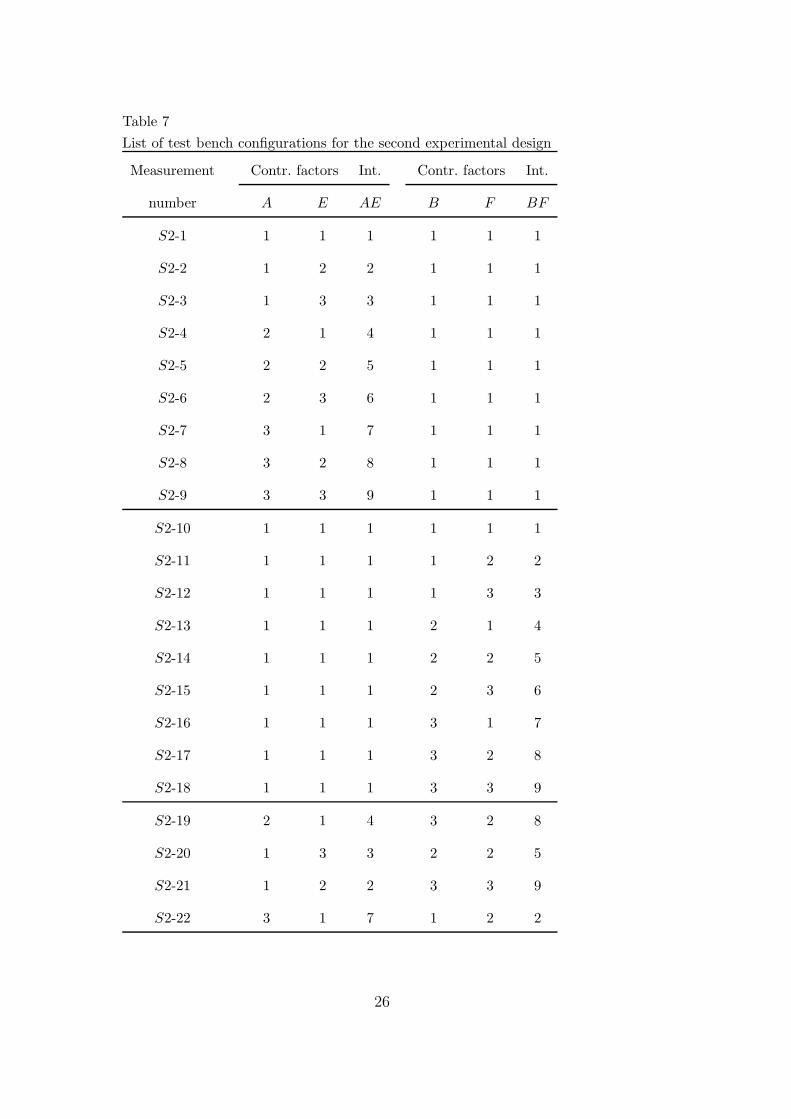
Table 7

List of test bench configurations for the second experimental design

Measurement Contr. factors Int. Contr. factors Int.

number A E AE B F BF

S2-1 1 1 1 1 1 1

S2-2 1 2 2 1 1 1

S2-3 1 3 3 1 1 1

S2-4 2 1 4 1 1 1

S2-5 2 2 5 1 1 1

S2-6 2 3 6 1 1 1

S2-7 3 1 7 1 1 1

S2-8 3 2 8 1 1 1

S2-9 3 3 9 1 1 1

S2-10 1 1 1 1 1 1

S2-11 1 1 1 1 2 2

S2-12 1 1 1 1 3 3

S2-13 1 1 1 2 1 4

S2-14 1 1 1 2 2 5

S2-15 1 1 1 2 3 6

S2-16 1 1 1 3 1 7

S2-17 1 1 1 3 2 8

S2-18 1 1 1 3 3 9

S2-19 2 1 4 3 2 8

S2-20 1 3 3 2 2 5

S2-21 1 2 2 3 3 9

S2-22 3 1 7 1 2 2

26

Table 8

Analysis of variance for the two L9 designs

Variation dof Sum of squares Mean squares F Contribution

A 2 1.95 0.97 147.09*** 62.64%

E 2 0.07 0.04 5.46** 1.91%

AE 4 0.23 0.06 8.84*** 6.72%

Residual 126 0.83 0.01 28.73%

Total 134 3.09

B 2 4.17 2.08 165.22*** 58.06%

F 2 0.67 0.33 26.52*** 9.02%

BF 4 0.71 0.18 14.05*** 9.23%

Residual 126 1.59 0.01 23.69%

Total 134 7.13

**p < .01; ***p < .001

27