influence of vertical earthquake motion stress response

99

Editor’s quick points

n Despite their proven benefits, precast concrete segmental bridges are rarely constructed in seismic regions of the United States.

n This paper investigates the seismic response of precast concrete segmental bridges constructed using the balanced-cantilever method using detailed two-dimensional, nonlinear time-history analyses and focuses on the behavior of segment-to-segment joints.

n This study indicates that vertical earthquake motions and the pre-earthquake stress state can significantly alter the response of segment joints.

Influence of vertical earthquake motion and pre-earthquake stress on joint response of precast concrete segmental bridgesMarc J. Veletzos and José I. Restrepo

Segmental construction methods using precast concrete can ease bridge construction costs by reducing construc-tion time while maintaining quality. In addition, the absence of falsework can minimize environmental impact and traffic congestion, adding to the benefits of this con-struction method. With more than 43,000 urban bridges in the United States (about one in three urban bridges) cur-rently classified as either structurally deficient or function-ally obsolete,1 the need is evident for accelerated bridge construction methods to open new routes and replace exist-ing structures with minimal traffic disruption.

While the popularity of precast concrete segmental bridge construction has increased throughout the world, its use in seismic regions of the United States has been hampered

PCI Journal | Summer 2009

Summer 2009 | PCI Journal100

Does the joint opening alter the serviceability of the • bridge?

Do volumetric changes, such as creep and shrinkage, • affect the joint response?

These questions have hampered owners’ use of precast concrete segmental bridges in seismic regions of the United States, namely California.

Research objectives

The large-scale experiments on the seismic response of precast concrete segmental bridge superstructures by Megally et al.,2 Densley et al.,3 and Burnell et al.4 deter-mined the crack patterns, failure modes, and ultimate be-havior of precast concrete segmental bridge superstructure joints. This paper provides additional information about seismic demands on the development of performance limit states in this type of construction.

Segment joint opening and the contribution of vertical earthquake motions

Burnell et al. showed experimentally that precast concrete segment joints open if vertical accelerations of 0.75g, where g is the acceleration due to gravity, develop in the superstructure and the superstructure post-tensioning is reduced 25%, indicating that vertical motion contributes to joint opening. However, this contribution by vertical motion was not decoupled from the effect of reducing the longitudinal post-tensioning.

The research program presented in this paper quantified the impact of vertical earthquake motion on the segment-joint response, determined whether segment joints are likely to open when full longitudinal post-tensioning is considered, and quantified the magnitude of the crack width when joints did open.

Performance limit states

Burnell et al. suggested that current seismic design procedures, based on capacity-design principles, prevent residual joint opening and protect the longitudinal post-tensioning tendons from yielding when vertical earthquake motion is not considered. However, there was no test to determine if this remains true when vertical earthquake motions are considered.

The research program presented in this paper compares the segment-joint response to concrete and post-tensioning performance limit states, such as cracking, crushing, and yielding; assesses the level of joint damage during a seis-mic event; and quantifies residual crack widths.

by a lack of research on the seismic response. The Cali-fornia Department of Transportation (Caltrans) supported a research program to address this concern. This research investigated the seismic response of precast concrete seg-mental bridges with bonded tendons constructed with the balanced-cantilever construction method.

Detailed, two-dimensional (2-D), nonlinear time-history analyses were used to conduct this research. A number of models were developed, including a segment-joint valida-tion model, for two balanced-cantilever precast concrete segmental bridges: one with a medium span and one with a large span. The bridges had span lengths of 300 ft and 525 ft (91 m and 160 m), respectively. While a number of parameters were studied, this paper focuses on the influ-ence of vertical earthquake motion and pre-earthquake stress on the seismic response of segment joints in the 300-ft-span bridge.

Benefits of segmental construction

The primary benefit of segmental bridges is that they can be constructed without temporary supports or falsework. Thus, segmental bridges are most effective for locations where falsework is expensive or impractical, such as deep ravines, wide water crossings, highly congested urban areas, and environmentally sensitive regions.

Precasting the concrete segments can add to the general benefits of segmental bridge construction by improving quality control, reducing creep and shrinkage deforma-tions, reducing weather’s effect on production rates, and improving construction speed.

Seismic concerns

The primary concerns regarding precast concrete segmen-tal construction subjected to seismic events are focused on the behavior of joints between segments because no mild-steel reinforcement crosses such joints. The lack of reinforcement across segment joints allows for an in-creased rate of construction but creates inherent regions of weakness that act as crack initiators and can result in localized rotations.

In recent years, bridge owners such as Caltrans have questioned the response of segment joints during a seismic event. Owners have asked questions such as:

Do these joints open during an earthquake? •

Do they remain open after the earthquake? •

Does the joint opening affect shear transfer across the • joints, thereby affecting dead-load-carrying capacity?

101PCI Journal | Summer 2009

Pre-earthquake stress state

The state of stress on segment joints changes on a daily basis because of temperature and over the life of the bridge because of volumetric effects such as creep and shrink-age. Typically, volumetric changes have been considered

unimportant and therefore have been ignored for seismic-design considerations. This is because the focus of seismic studies in the past has been on the ductility demand once the flexural strength of a component develops. At this limit state, volumetric changes play a minor role. However, the focus of this work is on the development of multiple per-

Table 1. Summary of earthquake ground-motion records

Earthquake Station Abb. Date Mw

Rupture surface

distance, mi

Scale factor

PGA horizontal,

g

PGA vertical,

g

Duration, sec

Component

Chi Chi, Taiwan TCU065 T65 9/20/1999 7.6 1.0 1.240 0.75 0.34 71.0 North-south

Chi Chi, Taiwan TCU068 T68 9/20/1999 7.6 1.1 1.156 0.54 0.57 71.0 North-south

Duzce, Turkey Bolu BOL 11/12/1999 7.1 7.5 2.592 1.91 0.54 50.0 North-south

Erzincan, Turkey Erzincan ERZ 3/13/1992 6.7 1.8 1.917 0.95 0.48 21.0 East-west

Tabas, Iran Tabas TAB 9/16/1978 7.4 3.0 1.358 1.15 0.95 32.0 North-south

Irpinia, Italy Calitri CAL 11/23/1980 6.5 5.5 5.355 0.95 0.79 40.0 North-south

Kobe, Japan Takarazuka TAK 1/16/1995 6.9 1.2 4.930 1.07 0.67 30.0 North-south

Kobe, Japan Takatori TAT 1/16/1995 6.9 0.3 1.437 0.52 0.23 30.0 East-west

Kobe, Japan Kobe JMA KOB 1/17/1995 6.9 0.5 2.792 1.67 0.97 30.0 East-west

Landers, California Lucerne LUC 6/28/1992 7.3 1.1 2.306 1.68 1.95 45.0 East-west

Loma Prieta, California

Gilroy Historic Building

GIL 10/17/1989 7.0 6.8 3.591 1.02 0.54 30.0 East-west


Lexington Dam Abutment

LEX 10/17/1989 7.0 6.3 2.775 3.93 1.25 30.0 North-south


Los Gatos Presentation Center

LOS 10/17/1989 7.0 3.5 0.954 1.05 1.46 22.0 East-west


Saratoga Aloha Avenue

SAR 10/17/1989 7.0 8.3 5.311 1.72 2.12 30.0 East-west

North Palm Springs, California

Morongo Valley MOR 7/8/1986 6.0 10.1 2.984 0.66 1.35 20.0 North-south

Northridge, Cali-fornia

Rinaldi RIN 1/17/1994 6.7 7.1 1.262 1.06 1.08 15.0 North-south

Northridge, Cali-fornia

Sylmar SYL 1/17/1994 6.7 6.4 1.171 1.00 0.64 30.0 North-south

Northridge-01, California

Arleta ARL 1/17/1994 6.7 9.2 5.557 1.72 3.16 35.0 North-south

San Fernando, California

Pacoima Dam PAC 2/9/1971 6.6 2.8 1.501 1.88 1.07 20.0 North-south

Superstition Hills, California

Wildlife Lique-faction Array

WIL 11/24/1987 6.7 14.9 2.085 0.43 0.89 42.0 North-south

Note: Abb. = abbreviation; g = 9.81 m/s2; Mw = moment magnitude scale value; PGA = peak ground acceleration. 1 mi = 1.609 km.


motions that occur in nature, the scale factor used in the longitudinal ground motions was also used on the verti-cal ground motion. The Pacific Earthquake Engineering Research (PEER) Center also used this record scaling ap-proach in the PEER Testbed projects.6

The duration of each record was extended by 15 sec, allowing the bridge-model response to damp out so that residual joint rotations and pier drift ratios could be obtained. In addition, the two ground-motion components were assumed to act at all foundations simultaneously. That is, incoherent ground motions were not considered despite the fact that they may have a significant effect on these types of bridges. The study of the response of segmental bridges to incoherent vertical ground motions requires a significant effort in appropriately modeling the boundary conditions of the bridge and of radiation damp-ing. This was outside the scope of this project.

Figure 1 shows the results of this scaling method. The median spectrum of the longitudinal motion matches the design spectrum fairly well. The longitudinal PGA and the spectral response below 1.0 sec for one particular earth-quake record was extremely high and will not likely occur naturally. This record was selected based on its response near the natural period of the structure. The displacement response at a period of 2.5 sec was greater than the major-ity of other records. Thus, this record helped to push the median response closer to the design spectrum at periods above 2.0 sec.

Joint-model validation

To ensure that the full-bridge earthquake simulations ac-curately represent the physical world, the joint-modeling approach had to be validated with physical experiments. The computer software Ruaumoko was selected to cre-ate models because of its extensive library of nonlinear hysteretic and damping rules. Two detailed finite-element models of test unit 100-INT from the phase I experiment by Megally et al. were created using Ruaumoko.

These models were developed to emulate numerous physi-cal characteristics of the segment-to-segment joints. These characteristics included crushing of extreme concrete fibers, yielding of tendons at the true limit of proportional-ity, and energy dissipation due to bond slip of the grouted internal tendons. This modeling approach was similar to a fiber model at the segment joints with nonlinear elements for the concrete and the post-tensioning tendons across the segment joints.

Typically, nine concrete elements and three post-tension-ing elements per tendon were used to model the super-structure section across each segmental joint. This model-ing approach matched the experimental results well and is documented in greater detail in Veletzos.7

formance limit states. Thus, the research presented in this paper assesses the impact of the pre-earthquake stress state on the response of segment joints.

Earthquake excitations

The site location for the bridge models was assumed to be 6 mi (10 km) from a strike-slip fault capable of producing a moment magnitude 8 earthquake and a peak ground accel-eration (PGA) of 0.7g. In addition, the site was assumed to be situated on soil type D as defined by Caltrans.5 This type of soil maintains frequency content at higher periods and is thus critical for long-span bridge structures. The design spectrum was selected from the Caltrans Seismic Design Criteria (SDC)5 based on the chosen site characteristics and represented a seismic event with a 5% probability of exceedance in 50 years (about a 1000-year return period).

There are few existing records of moment magnitude 8 seismic events that also exhibit near-field effects (that is, fling and forward directivity) recorded within 15 mi (25 km) of the fault. Thus, it was necessary to select ground motions from records as close as possible to the design scenario and scale them up to the design spectrum. Twenty near-field records were selected as input into the bridge models with the goal of obtaining the median seismic responses. All records were from earthquakes of moment magnitude 6.7 or greater and from stations within 15 mi of the fault rupture surface. Several of the ground motions included significant near-field effects.

These records were representative of a typical govern-ing design scenario seismic event in California and were selected because they were from an earthquake scenario (in terms of magnitudes and distances) similar to the as-sumed design event for the bridge-model site and because they typically exhibited a modest amount of frequency content near the natural period of the bridge structures. Table 1 lists the earthquakes used and summarizes various parameters of each ground motion. These ground motions were amplitude scaled to match the design spectrum at the primary natural period of the structure in the longitudinal direction.

The period of the fundamental longitudinal mode for both the 300-ft-span (91 m) bridge and the 525-ft-span (160 m) bridge was 2.0 sec. The longitudinal response of the bridge models may be greatly affected by the presence of the abutments after closure of the thermal expansion gap and engaging the abutment back wall. The fundamental period of vibration found from the modal analysis did not consid-er the bridge-abutment interaction, but the nonlinear model of the bridge did consider this interaction.

The current bridge design codes provide little guidance on the development of a vertical design spectrum. Thus, to keep the components of the seismic event consistent with


Figure 1. Earthquake response spectra illustrate the accelerations and displacements resulting from the scaling method. Note: g = acceleration due to gravity = 32.2 ft/sec2 = 9.8 m/sec2; PGA = peak ground acceleration. 1 in. = 25.4 mm.

0.0

1.0

2.0

3.0

4.0

5.0

6.0

7.0

8.0

0.0Period T, sec

Median

84th percentile

16th percentile

0.0

1.0

2.0

3.0

4.0

5.0

6.0

7.0

8.0

0.0

Acc

eler

atio

n S

A, g

Acc

eler

atio

n S

A, g

Dis

plac

emen

t SD, i

n.

2.01.51.00.5 2.5 3.0 3.5 4.0

Median

84th percentile

16th percentile

Magnitude 8 - soil type D - PGA = 0.7g

Longitudinal acceleration

0.0

0.5

1.0

1.5

2.0

2.5

3.0

3.5

4.0

4.5

5.0

Period T, sec

0.0

0.5

1.0

1.5

2.0

2.5

3.0

3.5

4.0

4.5

5.0

Median

84th percentile

16th percentile

Vertical acceleration

0

10

20

30

40

50

60

70

80

Period T, sec

Median

84th percentile

16th percentile

0

10

20

30

40

50

60

70

80Median

84th percentile

16th percentileMagnitude 8 - soil type D - PGA = 0.7g

Longitudinal displacement

0.00.0 0.50.40.30.20.1 0.6 0.7 0.8 0.9 1.0

0.00.0 2.01.51.00.5 2.5 3.0 3.5 4.0


integration time step was kept at a small 0.001 sec based on a parametric study.

Model discretization

The model consisted of 1228 nodes, 1637 elements, and 119 member properties. It was based on the Otay River Bridge in San Diego County, Calif., which opened to traf-fic in November 2007.8 The Otay River Bridge is 0.6 mi (1 km) long and consists of 4 longitudinal frames and a total of 11 tapered piers. The superstructure segments are 36 ft (11 m) wide and vary in depth from 10 ft (3 m) at midspan to 16 ft (5 m) at the piers. Thus, the span-to-depth ratio varies from 19 to 30.

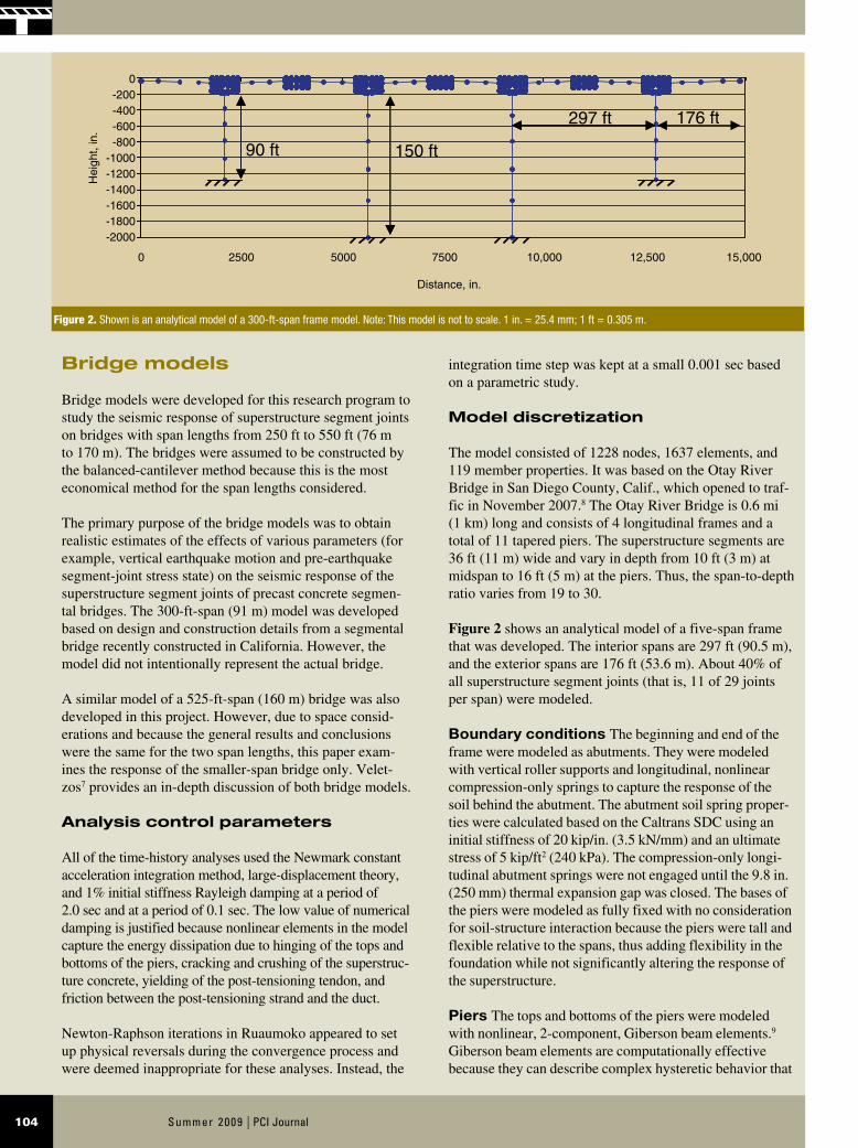
Figure 2 shows an analytical model of a five-span frame that was developed. The interior spans are 297 ft (90.5 m), and the exterior spans are 176 ft (53.6 m). About 40% of all superstructure segment joints (that is, 11 of 29 joints per span) were modeled.

Boundary conditions The beginning and end of the frame were modeled as abutments. They were modeled with vertical roller supports and longitudinal, nonlinear compression-only springs to capture the response of the soil behind the abutment. The abutment soil spring proper-ties were calculated based on the Caltrans SDC using an initial stiffness of 20 kip/in. (3.5 kN/mm) and an ultimate stress of 5 kip/ft2 (240 kPa). The compression-only longi-tudinal abutment springs were not engaged until the 9.8 in. (250 mm) thermal expansion gap was closed. The bases of the piers were modeled as fully fixed with no consideration for soil-structure interaction because the piers were tall and flexible relative to the spans, thus adding flexibility in the foundation while not significantly altering the response of the superstructure.

Piers The tops and bottoms of the piers were modeled with nonlinear, 2-component, Giberson beam elements.9 Giberson beam elements are computationally effective because they can describe complex hysteretic behavior that

Bridge models

Bridge models were developed for this research program to study the seismic response of superstructure segment joints on bridges with span lengths from 250 ft to 550 ft (76 m to 170 m). The bridges were assumed to be constructed by the balanced-cantilever method because this is the most economical method for the span lengths considered.

The primary purpose of the bridge models was to obtain realistic estimates of the effects of various parameters (for example, vertical earthquake motion and pre-earthquake segment-joint stress state) on the seismic response of the superstructure segment joints of precast concrete segmen-tal bridges. The 300-ft-span (91 m) model was developed based on design and construction details from a segmental bridge recently constructed in California. However, the model did not intentionally represent the actual bridge.

A similar model of a 525-ft-span (160 m) bridge was also developed in this project. However, due to space consid-erations and because the general results and conclusions were the same for the two span lengths, this paper exam-ines the response of the smaller-span bridge only. Velet-zos7 provides an in-depth discussion of both bridge models.

Analysis control parameters

All of the time-history analyses used the Newmark constant acceleration integration method, large-displacement theory, and 1% initial stiffness Rayleigh damping at a period of 2.0 sec and at a period of 0.1 sec. The low value of numerical damping is justified because nonlinear elements in the model capture the energy dissipation due to hinging of the tops and bottoms of the piers, cracking and crushing of the superstruc-ture concrete, yielding of the post-tensioning tendon, and friction between the post-tensioning strand and the duct.

Newton-Raphson iterations in Ruaumoko appeared to set up physical reversals during the convergence process and were deemed inappropriate for these analyses. Instead, the

Figure 2. Shown is an analytical model of a 300-ft-span frame model. Note: This model is not to scale. 1 in. = 25.4 mm; 1 ft = 0.305 m.

Distance, in.

0-200-400-600-800

-1000-1200-1400-1600-1800-2000

2500

90 ft 150 ft

297 ft 176 ft

5000 7500 10,000 12,500 15,0000

Hei

ght,

in.


is typical of reinforced concrete members using lumped plasticity. The Clough hysteresis rule was used to model the plastic hinging of the columns. The moment capacity of the piers was determined based on moment-curvature analyses using the program XTRACT. The plastic hinge lengths Lp of the piers were determined by

Lp = 0.08L + 0.3D + 0.15fydbl (1)

where

L = length of column shear span

D = depth of the column

fy = yield strength of mild-steel reinforcement

dbl = diameter of the longitudinal reinforcement bars of the column

This equation was developed by Hines et al.10 based on large-scale experiments of structural walls with confined corner elements, which were part of a larger research proj-ect studying the behavior of hollow columns with confined corner elements.

The Clough hysteretic rule did not capture the axial force-bending moment interaction of the columns. Because the focus of this investigation was the response of seg-ment joints, and the longitudinal moment demand on the superstructure is generated by the moment at the top of the column, it was important to subject the superstructure to the largest reasonable column moment. This moment oc-curs when the axial load on the column is at its maximum. Thus, the moment capacity of the piers was increased 25% above the dead-load moment capacity to account for vertical earthquake motion increasing the axial force on the piers, which increases the moment capacity of the piers. The 25% increase was based on a preliminary run of the model using vertical and lateral components of 100% of

the Rinaldi record from the 1994 Northridge earthquake in California.

Superstructure joints Figure 3 shows a typical pier cantilever for a 300 ft (91 m) span. Twenty-eight super-structure segments form the 300 ft span, so each span has 29 segment joints.

Eleven of these segment joints were modeled, six segment joints at each pier and five segment joints at midspan (Fig. 4). These joints were modeled in a manner similar to the validation models discussed previously and were con-sidered to be epoxied together. This allowed the joints to resist tension until cracking of the section occurred.

Nonlinear shear deformations of the superstructure were neglected because the shear spans were large (that is, M/V > 70 ft [21 m], where M is moment and V is shear) and, thus, shear deformations would be small. Cracking of the segments between joints was also neglected in order to simplify the model. This approach was justified by large-scale experimental results2–4 that indicated that very little, if any, flexural cracking occurred between segment joints.

Superstructure tendons To ensure that the forces in the tendons were realistic, the tendons were preloaded in the model according to the jacking forces required in the design. The model inherently accounted for elastic shorten-ing losses but not for losses due to friction or anchorage seating. To address this issue, the post-tensioning losses due to friction and anchorage seating were estimated for all tendons based on the provisions outlined in sec-tion 9.16 of the American Association of State Highway and Transportation Officials (AASHTO) Standard Specifications for Highway Bridges.11

The losses for all tendons crossing a joint were averaged and the pretension load reduced accordingly. For example, 14 cantilever tendons crossed the joint closest to the pier (that is, joint D1 or U1). The average loss in the post-

Figure 3. This diagram illustrates a common segment-joint-naming scheme for pier cantilevers. Note: The segment joints are numbered sequentially beginning near the pier and increasing both upstation and downstation toward midspan.

D14 D13 D2D3

Midspan

D1 U1 U2

Pier segmentElevation

U3 U13

Midspan

U14


tensioning member in the model was thus the average loss of all 14 tendons and was 17.8 ksi (123 MPa). This approach was used for all joints in the model. The losses ranged from 16 ksi to 21 ksi (110 MPa to 145 MPa), de-pending on the joint. Time-dependent losses such as creep, shrinkage, and relaxation were not inherently considered in the analyses, but they were considered separately, as discussed in following sections.

Pre-earthquake segment-joint stress state One of the parameters of interest in this research project was the impact of the pre-earthquake stress state on the response of segment joints. The pre-earthquake stress state of the structure depends on the construction method, creep, shrinkage, and temperature variations.

Creep and shrinkage depend on a number of variables, such as the compression stress on the section, the age of the concrete when the stress is applied, the duration of the load, and the relative humidity. A detailed analysis would be required to accurately estimate the effect of all of these variables on a structure in which every segment was constructed at different times, and the loading at each segment joint changed during the construction process. Thus, results from a full longitudinal construction staging analysis (LCSA) were used to find appropriate segment-joint pre-earthquake stress states.

Calibration process Figure 5 shows a comparison of the top and bottom superstructure stresses, at the end of construction, between the analytic model developed in this study and the designers’ LCSA calculations. The model

Figure 4. These diagrams show the modeling discretization for pier and midspan superstructure segment joints for the the 300-ft-span (100 m) model. Note: 1 in. = 25.4 mm.

Distance (in)

Bottom PT

Distance (in)Distance (in)

Bottom PT

Distance (in)Distance (in)Distance (in)Distance (in)Distance, in.

Hei

ght,

in.

Hei

ght,

in.

D30

-50

-100

-150

-200

-250

-300

0

-20

-40

-60

-80

-100

-120

-140

D2

1700 1800 1900 2000 2100 2200 2300 2400 2500

3400 3500 3600 3700 3800 3900 4000 4100 4200 4300

D1 U1 U3 U3

U13 U14 Midspan D14 D13

Bottom tendon

Columncenterline

Superstructuregirders

Top tendon

Adjacent to piers

Near midspan

Segment-to-segment joint

(three flange springs,three web springs)

Distance, in.


The bridge was constructed using the balanced-cantilever construction method. In this method, the superstructure behaves as a cantilever until continuity is built at midspan. Thus, this method results in large, negative dead-load bending moments at the pier faces (Fig. 6).

overestimated the top stress and underestimated the bot-tom stresses. This difference was caused by the effects of construction staging and indicates that the stress state in the superstructure is highly dependent on the method of con-struction.

Figure 5. These graphs compare the top and bottom superstructure stresses at the end of construction prior to calibration. Note: 1 in. = 25.4 mm; 1 ksi = 6.895 MPa.

Bottom fiber stresses

Top fiber stresses

0

0.0

-0.5

-1.0

-1.5

-2.0

-2.5

0.0

-0.2

-0.4

-0.6

-0.8

-1.0

-1.2

-1.4

2000 4000 6000 8000 10,000

Distance, in.

Distance, in.

Str

ess,

ksi

Str

ess,

ksi

TargetInitial model

TargetInitial model

12,000 14,000 16,000

0 2000 4000 6000 8000 10,000 12,000 14,000 16,000


To more accurately represent the stress state of the joints after construction, equal and opposite redistribution forces (that is, bending moments and axial forces) were applied across each segment joint in the analytical model (Fig. 7). The magnitude of these forces was iterated until conver-gence with the LCSA stress state was achieved. Figure 8 compares the top and bottom stresses at the end of con-struction and after the iteration process and indicates that the updated model matched the target end of construction stresses.

Considerations for variations in the pre- earthquake stress state Variables resulting in con-crete volumetric changes—namely creep, shrinkage, relax-ation, and temperature—influence the stress state of the segment joints continually over the life of the bridge. To investigate the effect of the pre-earthquake stress state on the seismic response, several pre-earthquake stress states were investigated. These stress states were developed in a systematic fashion based on the effect of creep and shrinkage.

The changes in the stress state due to creep and shrinkage of each segment joint were obtained from the LCSA. On average, the top- and bottom-fiber stresses lost compres-sion at the piers and at the bottoms of the midspan joints, while the compressive stresses increased in the top fibers of the midspan joints. This change in stress was used to generate four different pre-earthquake stress configurations that were intended to represent the range of stresses that might occur during the life of the superstructure. Table 2 shows the four pre-earthquake stress states considered.

Alternatively, the analytical model assumed that all con-crete was placed in a single placement operation and all tendons were stressed simultaneously on a fully continu-ous-frame structure. This generated significantly smaller negative dead-load bending moments at the piers and positive dead-load bending moments at midspan (Fig. 6). Such a model does not reflect the construction method, and staging must be adjusted to ensure accurate representation of the joint stress state.

Figure 7. This sketch shows the applied segment-joint forces required to calibrate the models. Note: M = moment; P = load.

P PM M

Bottom tendon

Top tendonConcretesprings

Superstructuregirders

Figure 6. The dead-load bending-moment diagram for balanced-cantilever construction is compared with that for the continuous-frame analytical model.

Pier PierPier Pier

Balanced-cantilever construction

Pier PierPier Pier

Continuous-frame analytical model


Table 2. Pre-earthquake stress states

Pre-earthquake stress state Description

–CS

This is the stress at the end of construction minus the change in stress due to creep and shrinkage. This stress configuration represented a potential state of stress near the end of construction—that is, beginning of service life—with considerations for possible inaccuracies in the LCSA as well as for considerations for the effect of temperature, particularly temperature gradients, on the bridge superstructure.

EOCThis is the best estimate of the stress state at the end of construction and considers construction staging effects as well as volumetric changes that occur during construction.

+CSThis is the best estimate of the state of stress after the majority of creep and shrinkage have occurred—that is, after about 10 years of service.

+2CS

This is the stress at the end of construction plus twice the change in stress due to creep and shrinkage. This stress configuration represented a potential stress state after 10 years of service life with considerations for possible inac-curacies in the LCSA and creep and shrinkage calculations as well as for considerations for the effect of temperature on the bridge superstructure.

Note: LCSA = longitudinal construction staging analysis.

Figure 8. These graphs compare the top and bottom superstructure stresses after calibration of the model to the end-of-construction stresses. Note: 1 in. = 25.4 mm; 1 ksi = 6.895 MPa.

Top fiber stresses

TargetUpdated model

Bottom fiber stresses

Str

ess,

ksi

S

tres

s, k

si

TargetUpdated model

0.0

-0.2

-0.4

-0.6

-0.8

-1.0

-1.2

0.0

-0.5

-1.0

-1.5

-2.0

-2.5

Distance, in.

Distance, in.

0 2000 4000 6000 8000 10,000 12,000 14,000 16,000

0 2000 4000 6000 8000 10,000 12,000 14,000 16,000


Figure 9. These graphs represent typical dead-load segment-joint stress profiles. Note: –CS = stress at end of construction minus the change in stress due to creep and shrinkage; +CS = stress at end of construction plus the change in stress due to creep and shrinkage; +2CS = stress at end of construction plus twice the change in stress due to creep and shrinkage; EOC = stress at end of construction; NA = neutral axis. 1 in. = 25.4 mm; 1 ksi = 6.895 MPa.

Stress, ksi

-4.0 -3.0 -2.0 -1.0 -0.0

Stress, ksi

-4.0

120

80

40

0

-40

-80

-120

80

40

0

-40

-80

-120-3.0 -2.0 -1.0 -0.0

Span 2 Pier 2

Dis

tanc

e fr

om N

A, i

n.

Dis

tanc

e fr

om N

A, i

n.

Stress, ksi

-4.0 -3.0 -2.0 -1.0 -0.0

Stress, ksi

-4.0

120

80

40

0

-40

-80

-120

80

40

0

-40

-80

-120

-3.0 -2.0 -1.0 -0.0

Span 2 Pier 2

Dis

tanc

e fr

om N

A, i

n.

Stress, ksi-4.0

120

80

40

0

-40

-80

-120-3.0 -2.0 -1.0 -0.0

Pier 2

Dis

tanc

e fr

om N

A, i

n.

Stress, ksi-4.0

120

80

40

0

-40

-80

-120-3.0 -2.0 -1.0 -0.0

Pier 2

Dis

tanc

e fr

om N

A, i

n.

Dis

tanc

e fr

om N

A, i

n.

Stress, ksi-4.0 -3.0 -2.0 -1.0 -0.0

80

40

0

-40

-80

-120

Span 2

Dis

tanc

e fr

om N

A, i

n.

Stress, ksi-4.0 -3.0 -2.0 -1.0 -0.0

80

40

0

-40

-80

-120

Span 2

Dis

tanc

e fr

om N

A, i

n.

-CS pre-earthquake stress state

EOC pre-earthquake stress state

Joint U13Joint U14MidspanJoint D14Joint D130.45f'c



Joint U13Joint U14MidspanJoint D14D130.45f'c

Joint D3Joint D2Joint D1Joint U1Joint U2Joint U30.45f'c




+CS pre-earthquake stress state

+2CS pre-earthquake stress state


Figure 10. These graphs illustrate the primary mode shapes. Note: T = period. 1 in. = 25.4 mm.

1000

500

0

-500

-1000

-1500

-20000 2000 4000 6000 8000

T = 0.32 sec

0% longitudinal mass22% vertical mass

12,00010,000 14,000 16,000

Hei

ght,

in.

1000

500

0

-500

-1000

-1500

-2000

Hei

ght,

in.

200

0

-200

-400

-600

-800

-1000

-1200

-1400

-1600

-1800

Hei

ght,

in.

Distance, in.

Vertical – mode 8

Vertical – mode 4

Longitudinal

0 2000 4000 6000 8000 12,00010,000 14,000 16,000

Distance, in.

0 2000 4000 6000 8000 12,00010,000 14,000 16,000

Distance, in.

T = 0.53 sec


T = 2.04 sec



ranged from 20% to 14% of fc' , while the average compres-

sion stress near midspan ranged from 16% to 8% of fc' .

Mode shapes Figure 10 depicts relevant mode shapes of the idealized bridge. The primary longitudinal mode had a period of 2.0 sec and a modal mass of 86% of the total bridge mass. This mode assumes no active engagement with the abutments.

Because the abutments will likely be engaged during strong shaking once the 9.8-in.-thick (250 mm) thermal expansion gap closes, the period obtained from the modal analysis is practically meaningless because it cannot be used to estimate the seismic response of the bridge. A more meaningful estimate of the actual period can be obtained using an iterative approach based on the secant stiffness and the tributary mass of the superstructure. The periods of the dominant vertical modes were 0.5 sec and

Model characteristics

Dead-load joint stresses The stress state in the segment joints before a seismic event likely affects the response of the joint. Figure 9 shows the stress profiles of the segment joints at pier 2 and span 3 for the four differ-ent pre-earthquake stress configurations. These profiles included dead load; post-tensioning loads; and losses due to elastic shortening, creep, shrinkage, relaxation, friction, anchorage seating, and the effects of construction staging. The stress profiles were typical of all segment joints in the model and were considered reasonable.

The peak stresses were well below the AASHTO limit of 0.45

fc' , where

fc' is the compressive strength of con-

crete.12 Table 3 shows the average compression stresses across the joints as a percentage of

fc' . The average com-

pression stress for segment joints adjacent to the piers

Table 3. Summary of average superstructure compression stress

Pre-earthquake stress configuration Adjacent to piers, % of f 'c Near midspan, % of f 'c

–CS 20 16

EOC 18 13

+CS 16 10

+2CS 14 8

Note: –CS = stress at end of construction minus the change in stress due to creep and shrinkage; +CS = stress at end of construction plus the change in stress due to creep and shrinkage; +2CS = stress at end of construction plus twice the change in stress due to creep and shrinkage; EOC = stress at end of construction; f 'c = compressive strength of concrete.

Figure 11. This graph shows the longitudinal push results. Note: 1 in. = 25.4 mm; 1 kip = 4.448 kN.

Top P2/P5Bottom P2/P5

Top P2/P5

Bottom P2/P5Top P3/P4

Bottom P3/P4

Top P2/P5Bottom P2/P5

Top P2/P5

Bottom P2/P5Top P3/P4

Abutment soil yield

Engage abutment

Bottom P3/P4

20,000

18,000

16,000

14,000

12,000

10,000

8000

6000

4000

2000

0

-2000

For

ce, k

ip

0 10 20 30 40 0 60 70

Displacement, in.

Total force

Column shears

Abutment forces


0.3 sec and captured 18% and 22% of the total bridge mass, respectively.

Longitudinal push results A longitudinal pushover analysis was performed to understand the hinging sequence of the frame (Fig. 11). It is clear that the abutment was engaged at 10 in. (250 mm) and just prior to hinging at the top of the short piers.

The onset of the nonlinear soil response behind the abut-ment occurred at about 13 in. (330 m). Hinging at the base of the short piers occurred shortly thereafter. The tall piers began to yield when the short piers reached an element displacement ductility of about 2. A 10 in. superstructure lateral displacement corresponded to a short pier drift of 1%.

Pier performance limit states Pier performance limit states were identified based on the longitudinal push-over and moment-curvature analyses of the pier sections using the program XTRACT. These limit states represent spalling of the cover concrete, crushing of the core con-

crete, first yielding of the reinforcement, full plastic hinge development, and fracture of the longitudinal bars. Table 4 summarizes the performance limit states, outlines the con-sequences of exceeding each limit state, and identifies the longitudinal drift ratio of piers 2 and 5 for each limit state. For convenience and simplicity, the drift ratios of the short-est pier were used to identify the limit states because the shortest piers were first in reaching these limit states.

Segment-joint behavior The segment-joint modeling approach was studied extensively and was validated with results from large-scale experiments. The predicted joint rotations from the model matched the measured rotations well. Veletzos7 documented the joint model validation in greater detail.

Segment-joint performance limit states Vertical pushover analyses were performed to obtain the backbone curve for the moment-rotation behavior of each segment joint and to identify the rotation where various performance limit states occurred. The limit states of interest were crack-

Table 5. Segment-joint performance limit states

Limit state Description Strain Consequences

C1 Concrete cracking εc = 0.000012 No onset of joint opening

C2 Spalling of extreme concrete fibers εc = -0.003Operational performance level: patching of concrete may be required

MT1Limit of proportionality of main tendons

εpt at fpt = 210 ksiOperational performance level: end of purely elastic region of post-tensioning and beginning of loss of prestressing force

MT2 Yield of main tendon εpt = 0.012Life-safety performance level: full tendon yielding, loss of significant post-tensioning force, residual joint openings likely

Note: fpt = stress in post-tensioning strand; εc = concrete strain; εpt = post-tensioning strand strain. 1 ksi = 6.895 MPa.

Table 4. Piers 2 and 5 performance limit states

Limit statePiers 2 and 5 drift

ratio, %Description Strain Consequences

P-C1 1.5 Spalling of cover concrete εc = -0.003Operational performance level: patching of concrete required

P-C2 5.7 Crushing of core concrete εc = -0.011Life safety performance level: fracture of confinement reinforcement and expensive repairs on short piers

P-R1 0.45First yield of longitudinal reinforcement

εs = 0.002 End of purely elastic region of reinforcement

P-R2 1.1 Idealized yield of section εs = 0.005Operational performance level: development of full plastic hinge, noticeable residual cracking, and pressure grouting possibly required

P-R3 4.3Fracture after buckling of longitudinal reinforcement

εs = 0.04Life safety performance level: expensive repairs on short piers

Note: εc = concrete strain; εs = reinforcing-steel strain.


ing of the section; onset of spalling of the extreme concrete fibers; the limit of proportionality of the main tendons, which was assumed to occur at a stress of 210 ksi (1450 MPa); and a strain of 1.2% in the main tendons. Table 5 outlines the con-sequences of the various performance limit states.

Vertical monotonic pushover analyses Figure 12 shows the backbone curves for the segment joints near midspan and limit states for the segments adjacent to the

piers. Table 6 summarizes the rotations at which the limit states were met for the various segment joints. Due to the regularity of the design and the gradual variations of the sections, the rotation limit states of the joints near the piers show only small variations. The same is true for the joints near the midspan.

Figure 12. The behavior of superstructure segment joints is shown for locations near the midspan and adjacent to the piers. Note: C1 = cracking limit state; C2 = spalling limit state; MT1 = limit of proportionality of the tendons; MT2 = full yielding of the main tendons. 1 kip-ft = 1.356 kN-m.

Rotation (miliradians)Rotation (miliradians)Rotation (miliradians)

0.5

0.0

-0.5

-1.0

-1.5

-2.0

-2.5

-3.0

-3.5

1.2

10.

0.8

0.6

0.4

0.2

0.0

-0.2

-0.4

-0.6

Mom

ent,

kip-

ft ×

105

Mom

ent,

kip-

ft ×

105

Rotation, mrad

Adjacent to piers

-2 -1 0 1 2 3

Rotation, mrad

Near midspan

-3 -2 -1 0 1 2 3

Joint D1/U1Joint D2/U2Joint D3/U3C1C2MT1MT2

Joint D133/U1Joint D14/U14MidspanC1C2MT1MT2


Figure 13. The bar graphs show the influence of vertical ground motion on the segment-joint rotations. Note: EOC = stress at end of construction; L_only = median response due to longitudinal only; L+V = median response due to both longitudinal and vertical ground motions. T = period.

14

12

10

8

6

4

2

0

0

-100

-200

-300

-400

-500

-600

-700

-800

-900

450

400

350

300

250

200

150

100

50

0

Res

idua

l rot

atio

n, µ

rad

Rot

atio

n, µ

rad

Rot

atio

n, µ

rad

Median residual rotations

T = 2 - EOC - L_onlyT = 2 - EOC - L + V



Median peak negative rotations

Median peak positive rotations

D1/U1 D2/U2 D3/U3 D13/U13 D14/U14 Midspan



Joint location

Joint location

Joint location


due to both longitudinal and vertical (that is, L+V) ground motions. The first graph in Fig. 13 plots the median peak-positive bending joint rotations for the six segment-joint families. D1/U1 represents the first joint down-station or up-station from the pier, while D14/D14 is 14 segment joints away from the pier and is adjacent to midspan (Fig. 3).

Adding the vertical ground-motion component signifi-cantly increased the joint rotation demand. By taking the median of the ratio of the L+V and L_only segment-joint median responses, the median positive bending rota-tions increased 1000%. From similar plots in Fig. 13, the median negative bending rotations increased 250% and the residual rotations remained essentially unchanged.

The reason for such large increases in the peak rotations can be explained by comparing the joint-rotation data with the performance limit states (Fig. 14). A different set of ground-motion records will likely have a different stan-dard deviation, which can alter the variation in the joint response presented here. Adding the vertical earthquake

Results of analyses

The impact of various parameters on the seismic response of segmental bridges, particularly the response of the superstructure segment joints, is presented in the follow-ing sections. The results are organized by the parameter of interest (that is, vertical excitation, pre-earthquake stress state, and the like) and by the span length.

Vertical excitation

To quantify the contribution of the vertical ground motion on the segment-joint response, the models were subjected to both longitudinal motions only and simultaneous longitudinal and vertical earthquake motions. The pre-earthquake joint-stress state was based on the best estimate of the stresses at the end of construction.

Figure 13 shows the effect of vertical excitation. The verti-cal bars in this figure represent the median response of the 20 earthquakes due to longitudinal only (that is, L_only) and

Figure 14. This graph illustrates the influence of vertical ground motion on positive midspan rotations. Note: Each small dot represents the peak rotation from one earth-quake. The square mark represents the median rotation. The diamond marks represent the 16th and 84th percentiles, and the vertical lines identify the various performance limit states. These percentile marks are shown to assess relative sensitivities based on the suite of ground-motion records used in this study. C1 = cracking limit state; C2 = spalling limit state; L_only = median response due to longitudinal only; L+V = median response due to both longitudinal and vertical ground motions; MT1 = limit of proportionality of the tendons; MT2 = full yielding of the main tendons.

Rotations, rad0.000001

L+V

C1 C2MT1 MT2L_only

0.00001 0.0001 0.001 0.01

Table 6. Summary of the rotational performance limit states

Segment joint


Performance limit state, mrad

C1Negative -0.024 -0.025 -0.025 -0.033 -0.034 -0.031

Positive 0.017 0.018 0.018 0.020 0.020 0.019

C2Negative -0.61 -0.73 -0.87 -1.66 -1.74 -1.98

Positive 1.38 1.43 1.52 1.84 1.89 2.44

MT1Negative -1.19 -1.15 -0.98 -1.32 -1.35 -1.27

Positive 2.52 2.70 2.69 1.43 1.50 1.47

MT2Negative -1.72 -1.71 -1.59 -2.16 -2.24 -2.16

Positive 4.50 3.64 5.01 2.32 2.37 2.31


a gap of 9 in. to 11 in. (230 mm to 280 mm) was estimated due to significant nonlinear response of the soil behind the abutment back wall. It was anticipated that this gap would be located between the superstructure and the abutment back wall. A gap of this size would significantly affect traf-fic flow and would likely require bridge closure for repair.

Pier response Figure 15 compares the median respons-es of the 20 earthquake records for the peak longitudinal drift ratios for the 4 pre-earthquake stress states. The peak longitudinal drift was unaffected by the pre-earthquake stress state of the superstructure segment joints.

Comparing the peak drifts of piers 2 and 5 (Fig. 15) with the longitudinal push results (Fig. 11) and performance limits (Table 4), the short piers developed full plastic hinges (that is, exceeded performance-limit state P-R1) and incipient spalling of cover concrete (that is, exceeded performance-limit state P-C2). This level of damage might not require closure of the bridge because the damage is below the roadway, but the bridge would require signifi-cant repair.

Superstructure segment-joint response Figure 16 compares the median segment-joint rotations among the various joint families for the four pre-earthquake stress states. The top graph in Fig. 16 presents the median response of the peak-positive-bending joint rotations. The pre-earthquake stress state affects the joint response, particularly near midspan, where the stress state at the end of construction plus twice the stress due to creep and shrinkage (+2CS) exhibited the largest rotations. This is because the bottom of the midspan joint was under the least amount of compression during the pre-earthquake stress

ground motions pushed the superstructure joints beyond the cracking limit state C1 and into the nonlinear range, where a small increase in bending moment produced a large increase in rotation.

The impact of vertical earthquake motion on the longitudi-nal response of the piers was negligible and is not present-ed in this paper.


The stress state of concrete bridges fluctuates on a daily basis because of temperature and over the service life of the bridge because of creep and shrinkage. The pre- earthquake stress state of the superstructure segment joints may affect the seismic response. To investigate this effect, four different pre-earthquake stress states were studied. These stress states represented the possible range of stress-es that might occur during the service life of a segmental bridge and are defined and discussed in Table 2.

The pre-earthquake stress state presented in this section used ground motions with both longitudinal and vertical components that were scaled based on the natural period of the bridge.

Abutment response Based on the Caltrans SDC strength and stiffness estimates of the soil behind the abut-ment back wall and considering the thermal expansion joint, the abutment soil will yield at a displacement of about 13 in. (330 mm). The peak abutment displacements were about 22 in. and 24 in. (560 mm and 610 mm) at abutments 1 and 6, respectively. The unloading response of the abutment soil was assumed to be equivalent to the initial stiffness. Thus,

Figure 15. This graph shows the influence of the pre-earthquake stress state on peak longitudinal drift ratio. Note: –CS = stress at end of construction minus the change in stress due to creep and shrinkage; +CS = stress at end of construction plus the change in stress due to creep and shrinkage; +2CS = stress at end of construction plus twice the change in stress due to creep and shrinkage; EOC = stress at end of construction; εc = concrete strain; εs = reinforcing steel strain.

First Yield εs = 0.002

T=2 - -T=2 - ET=2 - CT=2 - 2

T=2 - -T=2 - ET=2 - CT=2 - 2

-CSEOCCS2CS

T=2 - -T=2 - ET=2 - CT=2 - 2

T=2 - ET=2 - CT=2 - 2

-CSEOCCS2CS

-CS

EOCCS2CS

T=2 - ET=2 - CT=2 - 2

T=2 - ET=2 - CT=2 - 2

EOC+CS+2CS

2.5%

2.0%

1.5%

1.0%

0.5%

0.0%

Incipient spallingεc = 0.003

Full plastic hingeεs = 0.005

First yieldεs = 0.002

Drif

t rat

io, %

Pier 2 Pier 3 Pier 4 Pier 5Pier location


Figure 16. These graphs show the influence of the pre-earthquake stress state on segment-joint rotations. Note: –CS = stress at end of construction minus the change in stress due to creep and shrinkage; +CS = stress at end of construction plus the change in stress due to creep and shrinkage; +2CS = stress at end of construction plus twice the change in stress due to creep and shrinkage; EOC = stress at end of construction; L+V = median response due to both longitudinal and vertical ground motions; T = period.

1400

1200

1000

800

600

400

200

0

0

-200

-400

-600

-800

-1000

-1200

45

40

35

30

25

20

15

10

5

0

Rot

atio

n, µ

rad

Rot

atio

n, µ

rad

Res

idua

l rot

atio

n, µ

rad

D1/U1 D2/U2

Median peak positive rotations

Median peak negative rotations

Median residual rotations

D3/U3 D13/U13 D14/U14 Midspan



T = 2 - -CS - L+V

T = 2 - EOC - L+V

T = 2 - CS - L+V

T = 2 - 2CS - L+V

T = 2 - -CS - L+V

T = 2 - EOC - L+V

T = 2 - CS - L+V

T = 2 - 2CS - L+V

T = 2 - -CS - L+V

T = 2 - EOC - L+V

T = 2 - CS - L+V

T = 2 - 2CS - L+V

Joint location

Joint location

Joint location


Figure 17. These graphs illustrate the influence of pre-earthquake stress on joint D1/U1 rotations. Note: Each gray dot represents the peak rotation from one earthquake. The square marks represent the median rotation. The diamond marks represent the 16th and 84th percentiles, and the vertical lines identify the various limit states as defined in Table 2. C1 = cracking limit state; C2 = spalling limit state; –CS = stress at end of construction minus the change in stress due to creep and shrinkage; +CS = stress at end of construction plus the change in stress due to creep and shrinkage; +2CS = stress at end of construction plus twice the change in stress due to creep and shrinkage; EOC = stress at end of construction; MT1 = limit of proportionality of the main tendons; MT2 = full yielding of the main tendons.

Residual rotations

Residual rotations, rad

Peak negative rotations

Rotations, rad

0.000001

+2CS

+CS

EOC

-CS

+2CS

+CS

EOC

-CS

+2CS

+CS

EOC

-CS

C1

C1

C1

C2 MT2MT1

C2 MT2MT1

0.00001 0.0001 0.001 0.01

0.000001 0.00001 0.0001 0.001 0.01

Peak positive rotations

Rotations, rad

0.000001 0.00001 0.0001 0.001 0.01


median joint response that varied by as much as a factor of 10. The median joint response typically remained below both the concrete spalling limit state C2 and the limit of proportionality of the post-tensioning limit state MT1. Thus, loss of prestressing force did not occur. However, the extreme pre-earthquake stress states –CS and +2CS can develop extreme fiber stresses greater than 85% of

fc'

and, therefore, can develop significant microcracking. This microcracking resulted in small residual gaps that may re-quire repair. These residual gaps occurred most often near midspan, where the effects of creep and shrinkage were more pronounced.

While the results indicated that significant microcracking of the extreme superstructure fibers may occur (that is, concrete compressive stress was greater than 85% of

fc' , which translates to εc < –0.0016, where εc is concrete

strain), the damage in the short piers exceeded the spalling limit state (that is, εc < –0.003) and required more repair than the superstructure.

Superstructure segment-joint response summary Figure 19 summarizes the median positive, negative, and residual joint rotations for the worst-case pre-earthquake stress state on the monotonic push results. These figures also indicate the performance limit states. The approximate level of damage is also shown in these figures. In general, the first joint adjacent to the pier and the joint at midspan exhibited the largest rotation demands.

Design recommendations

Based on the results and conclusions presented previously, the following design recommendations are proposed.

Flange thickness

The top- and bottom-flange thickness must be large enough to ensure that the neutral axis of the superstructure does not migrate into the webs upon joint opening and crushing of the extreme concrete fibers. In other words, the top flange at the piers must be able to take the jacking force of the top and continuity tendons plus the yield force of the bottom tendons. Similarly, the bottom flange at the piers must be able to take the jacking force of the bot-tom tendons plus the yield force of the top and continuity tendons. This is also true for the midspan joints. This may be especially relevant under 3-D loading, where longitu-dinal and transverse seismic demands may generate large compressive demands on the corners of the cross section and confinement of the corners should be considered.

state +2CS, and it was the closest of the four pre-earthquake stress states to opening under positive bending.

The center graph in Fig. 16 presents the median response of the peak-negative-bending joint rotations. Once again, the midspan joints were the most affected by the pre-earthquake stress state, with the stress state at the end of construction minus the change in stress due to creep and shrinkage (–CS) generating the largest midspan rotations. This is because the top of the midspan joint was under the least amount of compression for stress state –CS and was closest to opening under negative bending.

The bottom graph in Fig. 16 presents the median response of the residual joint rotations. Near the piers there was a gradual increase in residual drift as the stress state moved from –CS to +2CS. This increase was relatively small, indicating that the joints closed completely for all stress states. Near midspan, the extreme stress states (–CS and +2CS) increased the median residual rotations significantly.

Figure 17 compares the peak rotations based on the four pre-earthquake stress conditions with the performance limit states for the first joint adjacent to piers D1/U1. The response of the other joints adjacent to the piers was simi-lar. In general, the median response for joint D1/U1 stayed below the spalling limit state C2 and the limit of propor-tionality of the tendons MT1. Thus, the response remained within the essentially elastic region and the segment joints returned to their pre-earthquake condition.

Figure 18 compares the peak rotations based on the four pre-earthquake stress conditions with the performance limit states for the midspan joints. The response of the other joints near midspan was similar. In general, the median response for the midspan joint remained below the spal-ling limit state C2 and the limit of proportionality of the tendons MT1. However, some nonlinear concrete material behavior did occur, resulting in residual rotations greater than the cracking limit state C1 (Fig. 18).

The bottom graph in Fig. 18 illustrates the impact of the pre-earthquake stress state on the residual midspan joint rotations. The median residual joint rotations of the extreme stress states, namely +2CS and –CS, were beyond the cracking limit state C1, indicating that the joint may maintain some amount of crack opening. These residual rotations were caused by extreme concrete-fiber stresses that exceeded 85% of

fc' and generated localized, nonlin-

ear deformations. The largest residual rotation occurred at midspan, where the dead load of the structure created a positive bending moment. Thus, the residual crack was below the bridge, not on the riding surface. This residual crack width remained small at less than 0.01 in. (0.25 mm).

In summary, the pre-earthquake stress state resulted in a


Figure 18. These graphs show the influence of pre-earthquake stress on midspan joint rotations. Note: C1 = cracking limit state; C2 = spalling limit state; –CS = stress at end of construction minus the change in stress due to creep and shrinkage; +CS = stress at end of construction plus the change in stress due to creep and shrinkage; +2CS = stress at end of construction plus twice the change in stress due to creep and shrinkage; EOC = stress at end of construction; MT1 = limit of proportionality of the main tendons; MT2 = full yielding of the main tendons.

C1C1

+2CS

+CS

EOC

-CS

+2CS

+CS

EOC

-CS

+2CS

+CS

EOC

-CS

C1

C1

C1

C2

C2

MT2

MT2

MT1

MT1

Residual rotations

Residual rotations, rad0.000001

0.000001

0.00001 0.0001 0.001 0.01

Peak negative rotations

Rotations, rad

0.00001 0.0001 0.001 0.01

0.000001

Peak positive rotations

Rotations, rad

0.00001 0.0001 0.001 0.01


or deflection of the bridge, it will likely be acceptable for seismic concerns as well.

Capacity design

Designers should continue using capacity-design prin-ciples to design precast concrete segmental superstructures because this approach appears to prevent permanent joint opening and yielding of the tendons adjacent to the piers. Capacity-design principles are essential to control the seismic performance of the column-superstructure con-nection. The current capacity-design approach considers overstrength of the column in the design of the superstruc-ture but does not consider the column axial force increase

Future post-tensioning tendons

While the results indicated that critical tendons were unlikely to exceed the full yield limit state, the possibility of loss of prestressing due to yielding of tendons warrants the recommendation that new segmental bridges allow for the possibility of future tendons in the design. The AASHTO Guide Specifications for Design and Construc-tion of Segmental Concrete Bridges12 require a provision for access and anchorage attachment of future tendons with a post-tensioning force not less than 10% of the posi-tive- and negative-moment primary post-tensioning forces. While this provision was intended to be an allowance for the addition of future dead load or to adjust for cracking

Figure 19. These graphs summarize the median joint response for worst-case, pre-earthquake stress state. Note: C1 = cracking limit state; C2 = spalling limit state; MT1 = limit of proportionality of the main tendons; MT2 = full yielding of the main tendons. 1 kip-ft = 1.356 kN-m.

1.2

1.0

0.8

0.6

0.4

0.2

0.0

-0.2

-0.4

-0.6

0.5

0.0

-0.5

-1.0

-1.5

-2.0

-2.5

-3.0

-3.5

Mom

ent,

kip-

ft ×

105

Mom

ent,

kip-

ft ×

105

Near midspan

Rotation, mrad-2 -1.5 -1 -0.5 0

Adjacent to the pier

Rotation, mrad0-0.5-1 0.5 1 1.5

0.5 1 1.5 2

MidspanJoint D14/U14Joint D13/U13C1C2MT1MT2NegativePositiveResidual

Joint D1/U1Joint D2/U2Joint D3/U3C1C2MT1MT2NegativePositiveResidual


segmental bridge superstructures and should be considered during the design process. At this time, it is recommended that the superstructure dead-load demands at the end of construction and after the majority of creep and shrinkage have occurred, as determined from a full longitudinal con-struction staging analysis, be combined with the vertical earthquake demands. Equations (2) and (3) are the recom-mended seismic-load combinations.

DLEOC + EQKVert (2)

DLCS + EQKVert (3)

where

DLCS = superstructure member dead-load forces based on consideration for creep and shrinkage losses

DLEOC = superstructure member dead-load forces based on end of construction stresses

EQKVert = superstructure member forces due to vertical earthquake loads

The peak vertical and horizontal earthquake demands are not likely to occur simultaneously, so horizontal earth-quake demands are not included in these load combina-tions. The authors recognize that Eq. (2) and (3) are load combinations that may result in design forces that have a return period that is larger than the return period of the design-level earthquake. These recommended seismic load combinations may be revised in the future pending the results of a full probabilistic assessment of Eq. (2) and (3).

Vertical earthquake demands The results showed that vertical earthquake ground motion can significantly increase the demands on segmental superstructures and should be considered in the design process. The recom-mended method to estimate the vertical earthquake demands depends on the design level (FEE or SEE) and the importance classification of the bridge (Table 8).

due to vertical excitation and the corresponding increase in the column moment capacity. This approach is not a truly rigorous capacity-design approach, but it appears to be acceptable and considerations for the effects of vertical earthquake motion on the column-moment capacity are not recommended for the capacity design of the superstructure. Capacity-design principles have no effect near midspan, so additional design requirements are necessary and are outlined in the next section.

Seismic design framework

A two-level design approach is recommended in which dif-ferent performance limits are required for different levels of earthquakes (Table 7). The recommended return period of these earthquake events varies depending on the bridge classification. This approach is compatible with current seismic design practice for important bridges.

For the lower-level functional evaluation earthquakes (FEE), it is recommended that the superstructure be de-signed such that the segment joints remain closed.

For a safety evaluation earthquake (SEE), the recommended design approach varies depending on the classification of the bridge. It is recommended that ordinary bridges be designed with a no-collapse criterion and important bridge structures be designed to remain undamaged. The superstructures of important bridges should be designed to allow joint open-ing while ensuring that the tendons remain elastic (that is, fpt < 0.78fu = 210 ksi, where fpt is the stress in the prestress-ing strand and fu is the ultimate strength of the prestressing strand) and that the concrete does not crush (that is, εc < 0.002).

Recommendations for the appropriate method to determine the vertical earthquake demands, segment-joint capacity, and load combinations that consider the pre-earthquake stress state are discussed in the following section.

Pre-earthquake stress state and load combinations The results indicated that the superstruc-ture pre-earthquake stress state can affect the response of

Table 7. Recommended seismic design framework

Bridge classification Functional evaluation earthquake Safety evaluation earthquake

Ordinary No joint opening: 100-year return period No collapse: 1000-year return period

Important No joint opening: 500-year return period Nonlinear elastic joint response: 2500-year return period

Table 8. Recommended modeling approach for vertical earthquake demands

Bridge classification Functional evaluation earthquake Safety evaluation earthquake

Ordinary Elastic modal analysis Check collapse mechanism

Important Elastic modal analysis Nonlinear time-history analysis


M

Midspan

+ = ultimate positive bending capacity of the midspan segment joint of interior spans

M Mid end-+ = ultimate positive bending capacity of the

middle segment joint of end spans

Li = length from the abutment centerline to the segment joint of interest

Pre-earthquake stress states do not need to be considered in the capacity of the collapse mechanisms because they will not significantly affect the ultimate capacity of the superstructure.

FEE design level of important bridges It is rec-ommended that the vertical earthquake demands for the FEE design level of important bridges be determined from a vertical modal analysis. However, given that a full 3-D, nonlinear time-history analysis is recommended for the SEE design level of important bridges, in practice it may be easier to use 3-D time-history analysis for the FEE runs as well. Time-history analysis is considered to be more real-istic than modal analysis and is considered appropriate for the FEE design level.

SEE design level of important bridges It is rec-ommended that the vertical earthquake demands for the SEE design level of important bridges be determined from 3-D, nonlinear time-history analysis based on appropri-ate horizontal and vertical ground motions. Appropriate vertical ground motions are considered to be ground motions that exhibit vertical-to-horizontal spectral ratios as described by Bozorgnia and Campbell.

It is recommended that the superstructure be modeled with nonlinear, elastic moment-rotation hinging elements at select segment joints. At a minimum, two segment joints adjacent to the piers and three segment joints near midspan should be modeled. The moment-rotation characteristics of each joint should be determined from local finite-element models.

Extreme pre-earthquake stress states of the segment joints must be considered based on the end-of-construction stresses, and the stresses after creep and shrinkage losses per Eq. (2) and (3). Thus, it is recommended that forces be applied across the nonlinear segment-joint members to calibrate the model to these pre-earthquake stress states.

Segment-joint capacity of ordinary bridges Moment-curvature analysis is recommended to determine the vertical capacity of the segment joints of ordinary bridges at cracking for the FEE design level and at ultimate capacity for the SEE design level. Expected concrete and prestressing material properties should be used in these calculations as outlined in the Caltrans SDC. The preload in the tendons should be based on the expected tendon force at

FEE design level of ordinary bridges It is rec-ommended that the vertical earthquake demands for the FEE design level of ordinary bridges be determined from a vertical modal analysis based on a design spectrum per Bozorgnia and Campbell.13 A sufficient number of modes should be considered in the modal analysis to capture at least 90% of the superstructure mass in the vertical direc-tion. It is recommended that these vertical earthquake demands be combined with dead load per Eq. (2) and (3).

SEE design level of ordinary bridges It is recom-mended that designers satisfy the no-collapse criteria for ordinary bridges by checking the capacity of all vertical col-lapse mechanisms relative to the vertical design spectrum. The collapse mechanism capacity Sc for both interior Sc,int and end spans Sc,end must be greater than the vertical PGA in the vertical design spectrum and can be determined based on Eq. (4) and (5).

Sc,int

=w

int

Wint

/ Lint

−1 (4)

Sc,end

=w

end

Wend

/ Lend

−1 (5)

where

Lend = clear end-span length

Lint = clear interior-span length

wend = uniform distributed load of the end-span segment

wint = uniform distributed load of the interior-span segment

Wend = total weight of the end-span segment

Wint = total weight of the interior-span segment

The uniform distributed loads wend and wint that will de-velop these collapse mechanisms can be determined from Eq. (6) and (7) for both end and interior spans.

wL L L

ML

LMend

end i iPier

i

endi=

−+− +8

4 4 2 ( ) (6)

wL

M MPier Midspanintint

= +( )− +82 (7)

where

M

Pier

− = ultimate negative bending capacity of the seg-ment joint adjacent to the pier


The results presented indicated that vertical earthquake motions significantly contributed to the joint response and increased the peak-negative-moment joint rotations more than 1000% and the peak-positive-moment rotations at least 250%, but they did not affect the residual rotations. Segment joints in positive bending near midspan experi-enced the largest rotation increases due to vertical ground motions. These large increases were generated because the vertical ground motion pushed the segment joints beyond the cracking limit state and into the nonlinear region.

Joint opening

The median segment-joint rotation results presented in this paper showed that the segment joints exceeded the cracking limit state and opened gaps at the extreme fibers of the superstructure during a significant seismic event. In general, the first joint adjacent to the pier and the joint at midspan exhibited the largest rotation demands. The 300-ft-span (91 m) model indicated that peak gap widths adjacent to the piers and near midspan may be up to 0.05 in. and 0.15 in. (1.3 mm and 3.8 mm), respectively.

Performance limit states

Vertical pushover analyses were performed to identify the rotations in which various performance limit states occurred. The limits states of interest were cracking of the section C1; spalling of the extreme concrete fibers C2; the limit of proportionality of the main tendons MT1, defined as a stress of 210 ksi (1450 MPa); and full yielding of the main tendons MT2, defined as a strain of 1.2%.

The time-history results showed that the response of the segment joints typically remained below the concrete spal-ling and the tendon limit of proportionality limit states. However, the concrete compressive stress did exceed 85% of

fc' and resulted in significant microcracking at select

segment joints, particularly at the top fibers at midspan due to positive bending. This excessive microcracking generated residual rotations at midspan that were larger than the crack-ing limit state. However, these residual rotations remained small, creating crack widths of less than 0.01 in. (0.25 mm). While the damage observed in the superstructure was relatively light and repairable, the damage at the piers was significantly more severe, exceeding the full plastic hinge limit state (εs > 0.005, where εs is the reinforcing steel strain) and the concrete spalling limit state (εc < –0.003).


The results indicated that the pre-earthquake stress state can influence the seismic response of segment joints and can create order-of-magnitude variations in rotational demands. This finding is contrary to the commonly ac-cepted viewpoint that volumetric changes have negligible effects on the structure’s response to earthquakes. While

the end of construction and after considering losses due to creep, shrinkage, and relaxation.

Segment-joint capacity of important bridges It is recommended that the vertical capacity of segment joints of important bridges be determined using detailed, local, nonlinear finite-element models based on the expected con-crete and prestressing material properties. These models must capture the nonlinear characteristics of the extreme concrete fibers in both tension and compression. In addition, the model must capture the nonlinear characteristics of the tendons with accurate estimates of the pretension forces.

It is recommended that these models be subjected to mono-tonic rotational push analyses to determine the moment-rotation characteristics of the segment joints. Cyclic push analyses are not required, so the hysteretic rules used for the concrete and post-tensioning members are unimportant. At this time, the unbonded length of the tendons Lu should be determined based on Eq. (8).

Lu = 0.625(fps – fpe) db (8)

where

fps = full design strength of post-tensioning strand

fpe = effective stress in post-tensioning strand

db = diameter of post-tensioning strand

Equation (8) is 50% of the flexural-debond-length equa-tion determined by Zia and Mostafa.14 A 50% reduction was used because the unbonded length used for model-ing of tendons is about half of the flexural debond length based on a strain energy comparison. Because Eq. (8) was determined based on tests of single-strand tendons, this approach will likely be a lower bound for designing multi-strand tendons, ensuring lower-bound rotation capacities.

Summary

This research project studied the seismic response of pre-cast concrete segmental bridges and had an emphasis on the behavior of superstructure segment joints constructed using the balanced-cantilever method. The primary research tool used in this investigation was detailed 2-D, nonlinear time-history analyses. The characteristics and results of only the 300-ft-span (91 m) model were presented due to space considerations.

Contribution of vertical earthquake motions

The full bridge models were subjected to both longitudinal ground motion only and simultaneous longitudinal and vertical ground motions to quantify the contribution of the vertical ground motion on the segment-joint response.


6. Pacific Earthquake Engineering Research (PEER) Center. PEER Testbeds Program. www.peertestbeds .net.

7. Veletzos, M. J. 2007. The Seismic Response of Pre-cast Segmental Bridge Superstructures with Bonded Tendons. PhD diss. University of California at San Diego.

8. Gale, Sarah Fister. 2008. Otay River Bridge. PCI Journal. V. 54, No. 6 (November–December): pp. 38–47.

9. Giberson, M. F. 1969. Two Non-linear Beams with Definitions of Ductility. Journal of the Structural Division, V. 95: pp. 137–157.

10. Hines, E. M., F. S. Seible, and M. J. N. Priestley. 1999. Cyclic Tests of Structural Walls with Highly-Confined Boundary Elements. SSRP 1999/15. Uni-versity of California at San Diego, La Jolla, CA.

11. American Association of State Highway and Trans-portation Officials (AASHTO). 2002. Standard Specifications for Highway Bridges. 17th ed. Wash-ington, DC: AASHTO.

12. AASHTO. 1999. Guide Specifications for Design and Construction of Segmental Concrete Bridges. 2nd ed. Washington, DC: AASHTO.

13. Bozorgnia, Y., and K. W. Campbell. 2004. The Vertical-to-Horizontal Response Spectral Ratio and Tentative Procedures for Developing Simplified V/H Vertical Design Spectra. Journal of Earthquake Engi-neering, V. 8, No. 2 (March): pp. 175–207.

14. Zia, P., and T. Mostafa. 1977. Development Length of Prestressing Strands. PCI Journal, V. 22, No. 5 (September–October): pp. 54–65.

Notation

db = diameter of the post-tensioning strand

dbl = diameter of the longitudinal reinforcement bars of the column

D = depth of column

DLCS = superstructure member dead-load forces based on consideration for creep and shrinkage losses

DLEOC = superstructure member dead-load forces based on end-of-construction stresses

the rotational demands typically remained below critical performance limit states, some pre-earthquake stress states, namely extreme stress states –CS and +2CS, caused ex-treme fiber compression stresses to exceed 85% of

fc' and

generated significant microcracking that resulted in small residual cracks.

Acknowledgments

This research project was made possible by funding from the California Department of Transportation under contract no. 59A0337. The input of Charly Sikorsky and others at Caltrans is greatly appreciated.

The authors express their gratitude to Athol Carr at the University of Canterbury in New Zealand for his assistance with developing a suitable finite-element model, Benjamin Soule and Daniel Tassin at International Bridge Technolo-gies for their assistance with design details of the Otay River Bridge, and Sajid Abbas at T. Y. Lin International for his assistance with design details of the San Francisco–Oakland Bay Bridge Skyway.

The authors appreciate the valuable and constructive com-ments of the PCI Journal reviewers.

References

1. U.S. Department of Transportation (USDOT). 2006. Research and Innovative Technology Administration, Bureau of Transportation, Statistics: Transportation Statistics Annual Report. Washington, DC: USDOT.

2. Megally, S. H., M. Garg, F. Seible, and R. K. Dowell. 2002. Seismic Performance of Precast Segmental Bridge Superstructures. Structural Systems Research Project (SSRP) 2001/24. University of California at San Diego, La Jolla, CA.

3. Densley, D., S. H. Megally, and F. Seible. 2003. Seismic Performance of Precast Segmental Bridge Superstructures with Lightly Stressed Continuity Tendons. SSRP-2003/10. University of California at San Diego, La Jolla, CA.

4. Burnell, K. P., S. H. Megally, J. I. Restrepo, and F. Seible. 2005. Seismic Testing of Precast Segmental Systems Bridges: Phase III, Bridge Systems Test. SSRP 2005/01. University of California at San Diego, La Jolla, CA (June).

5. California Department of Transportation (Caltrans). 2004. Seismic Design Criteria. Version 1.3. Sacra-mento, CA: Caltrans.


V = shear

V/H = vertical-to-horizontal spectral ratio

wend = uniform distributed load that develops col-lapse mechanisms on end span

wint = uniform distributed load that develops col-lapse mechanisms on interior spans

Wend = total weights of the end-span segments

Wint = total weights of the interior-span segments

εc = concrete strain

εpt = strain in post-tensioning strand

εs = reinforcing steel strain

EQKVert = superstructure member forces due to vertical earthquake loads

fc' = compressive strength of concrete

fpe = effective stress in post-tensioning strand

fps = full design strength of post-tensioning strand

fpt = stress in post-tensioning strand

fu = ultimate strength of prestressing strand

fy = yield strength of mild-steel reinforcement

g = acceleration due to gravity

L = length of column shear span

Lend = clear end-span length

Li = length from the abutment centerline to the seg-ment joint of interest

Lint = clear interior-span length

Lp = length of plastic hinge

Lu = unbonded length of a multistrand tendon

M = moment

M Mid end-+ = ultimate positive bending capacity of the

middle segment joint of end spans

M

Midspan

+ = ultimate positive bending capacity of the mid-span segment joint of interior spans

M

Pier

− = ultimate negative bending capacity of the seg-ment joint adjacent to the pier

Mw = moment magnitude scale value

P = load

SA = spectral acceleration

Sc = collapse mechanism capacity

Sc,end = exterior span collapse-mechanism capacity

Sc,int = interior span collapse-mechanism capacity

SD = spectral displacement

T = period


About the authors

Marc J. Veletzos, PhD, P.E., is an assistant professor of civil engineering at Merrimack College in North Andover, Mass.

Jose I. Restrepo, PhD, is a professor of structural engineer-ing at the University of California at San Diego.

Synopsis

Segmental construction of precast concrete bridges can accelerate construction and minimize the cost in highly congested urban environments, environmentally sensi-tive regions, difficult-to-access ravines, and wide river crossings where medium-sized to long repetitive spans are needed. Despite their proven benefits, precast concrete segmental bridges experience limited use in seismic regions of the United States. A main obstacle to their use is concern regarding the seismic response of segment joints.

This paper investigates the seismic response of precast concrete segmental bridges using detailed, two- dimensional, nonlinear time-history analyses and focuses on the behavior of segment-to-segment joints constructed using the balanced-cantilever method. Analytical models of full-scale precast concrete

segmental bridges with geometries and characteristics similar to the Otay River Bridge in California were used in this study.

Twenty near-field earthquake records were used to determine the median joint response as well as to quantify the effect of vertical motion on the joint re-sponse. Four different pre-earthquake stress conditions were studied to determine whether the effects of creep, shrinkage, and temperature affect the seismic response of segment joints.

Results indicated that vertical earthquake motions and the pre-earthquake stress state can significantly alter the response of segment joints.

Keywords

Bonded tendon, bridge, earthquake, external tendon, finite-element analysis, large-scale testing, nonlinear analysis, post-tensioning, segmental construction, seismic, superstructure.

Review policy

This paper was reviewed in accordance with the Precast/Prestressed Concrete Institute’s peer-review process.

Reader comments

Please address any reader comments to PCI Journal editor-in-chief Emily Lorenz at [email protected] or Precast/Prestressed Concrete Institute, c/o PCI Journal, 209 W. Jackson Blvd., Suite 500, Chicago, IL 60606. J

influence of vertical earthquake motion stress response

Documents