1

Influential analyst recommendations:

Are they the hidden gem?

José Afonso Faias and Pedro M. N. Mascarenhas

Current version: November 2013

Abstract

Informational signals play an important role in Finance. From an ex post exercise, there are 20%

influential analyst recommendations in terms of impact on the price. We perform a predicting

exercise to forecast influential recommendations changes. We find that ex ante these depend on

the magnitude of the recommendation change, concurrent earnings forecasts issued around the

recommendation change, and firm institutional ownership. From this knowledge, we construct

an out of sample long-short portfolio that buys positive and sells negative influential

recommendation changes’ stocks. This strategy yields a net annualized abnormal return of 26%,

an annualized Sharpe ratio of 1.23, and an annualized certainty-equivalent of 27% between 1999

and 2012, which compares well to an annualized Sharpe Ratio of 0.40 and an annualized

certainty-equivalent of 6% of the CRSP equally-weighted index.

2

1. Introduction

Every so often, market observers point significant share-price reaction to analyst

recommendation changes. On September 1st 2009 Todd Bault, from Bernstein, issued a

recommendation change (downgrade) warning investors to the fact that AIG’s share could be

worthless. Soon the share price fell approximately by 11%1. The shares of Suedzucker AG fell

12%2 and trading volumes exceeded the previous three-month daily average3, on September 3rd

2013, after the downgrade by Exane BNP Paribas, who predicts the end of regulated European

sugar market.

There is evidence that, during the period between 1965 and 1989, trading strategies long

on past winner and short on past loser stocks realize significant abnormal returns (Jegadeesh and

Titman, 1993). This is not due to systematic risk and can also not be attributed to delayed stock

price reactions to common factors. Still, there is evidence that firm-specific information causes

the delay in price reaction. Therefore, analyst recommendations, which are firm-specific, should

be able to provide some return to investors. According to Womack (1996), recommendation

changes to positive (negative) categories generate positive (negative) excess returns in the

direction of the analyst’s forecast predominantly during the period of one month (six months).

Barber et al. (2001) find that an investment strategy based on average analyst recommendations,

long on the buy recommendations and short on the sell recommendations, delivers positive

returns.

Loh and Stulz (2011) find that approximately 11.7% of the recommendation changes

analyzed are influential, which they define as an analyst recommendation change that has a

recognizable impact at the firm level. Our results show that the percentage of influential

1 Tibken, Shara. The Wall Street Journal. November 30, 2009. http://blogs.wsj.com/marketbeat/2009/11/30/aig-

shares-fall-as-bernstein-cuts-price-target/ 2 Morgan, Jonathan. Bloomberg. September 3, 2013. http://www.bloomberg.com/news/2013-09-03/german-stocks-

decline-as-thyssenkrupp-suedzucker-retreat.html 3 Zha, Weixin. Bloomberg Businessweek. September 3, 2013. http://www.businessweek.com/news/2013-09-

03/suedzucker-falls-as-end-to-eu-subsidies-beckons-frankfurt-mover

3

recommendations is actually greater, 19.4% for our sample. In our results we find stronger

evidence, which supports that after the implementation of the Fair Disclosure Regulation analyst

recommendations have a stronger impact. As we find a greater percentage of influential

recommendation changes between 2003 and 2012, compared to the recommendation change

during 1993 and 2002.

Using Loh and Stulz (2011) findings that there is a specific group of recommendation

changes that has a greater impact on the market and can be described by specific characteristics,

we perform a predicting exercise to forecast influential recommendations changes. We find that

ex ante these depend on the magnitude of the recommendation change, concurrent earnings

forecast, and firm institutional ownership. From this knowledge, we construct an out of sample

long-short portfolio that buys positive and sells negative influential recommendation changes’

stocks, similar to the one proposed by Womack (1996). This strategy yields a net annualized

abnormal return of 26%, an annualized Sharpe ratio of 1.23, and an annualized certainty-

equivalent of 27% between 1999 and 2012, which compares well to an annualized Sharpe Ratio

of 0.40 and an annualized certainty-equivalent of 6% of the CRSP equally-weighted index.

The rest of this paper is organized as follows. Section 2 describes the data used. Section 3

discusses the predictions of influential recommendation changes. Section 4 considers the results

of our proposed out of sample investment strategy and Section 5 considers various robustness

checks on our results. Finally Section 6 concludes.

2. Data & Methodology

2.1. Data

The stock recommendations sample is extracted from the Thomson Financial’s Institutional

Brokers Estimate (I/B/E/S) U.S Detail File. The sample is built starting from I/B/E/S ratings

issued by individual analysts from September 1993 to December 2012, with ratings ranging from

4

1 (strong buy) to 5 (sell). We use an inverted ratings scale, as in Loh and Stulz (2011) (e.g., strong

buy now denoted by 5).

The emphasis is on recommendation revisions and not levels, because previous research

has found that recommendation changes contain more information (e.g., Jegadeesh and Kim,

2010). The recommendation change, rec_chg, is computed as the difference between the current

rating and the previous outstanding rating by the same analyst. The rating changes level lies

between -4 and +4, as ratings are coded as 5 (strong buy) to 1 (sell). We use Ljungqvist, Malloy

and Marston (2009) definition that the rating has to have been confirmed by the analyst in the

last twelve months and has not been stopped by the broker, for outstanding rating. Analysts

coded as anonymous by I/B/E/S are removed as it is not possible to track their

recommendation revisions. Also, companies that have less than five recommendations during

the whole sample period and companies that have less than two years of stock price data in the

CRSP are removed. This reduces the number of companies to a total of 2,700 followed by 7,553

analysts. On average, we have recommendation changes for 991 companies/year. In 1993 we

start with 107 firms, as the I/B/E/S recommendation sample only starts during the 4th quarter

of 1993. In 1997, we have the most companies in a year, 1,227. The sample of recommendation

changes contains a total of 116,028 recommendation changes and almost 99% of these

recommendation changes lay within the range of -2 to +2. In Table I the transition probabilities

of the recommendation changes are plotted. We observe that recommendations are mainly in

optimistic levels and one can read that prior hold ratings are more often upgraded, while the

non-hold are revised to hold ratings.

We use the Recommendations Summary Statistics file from I/B/E/S to obtain the

recommendation consensus. To estimate the analyst’s forecast accuracy we get the one year

earnings forecast (FY1) and actual earnings for the forecasted year from the detailed earnings

forecast file from I/B/E/S. We also retrieve the target price data from the I/B/E/S. Each target

price specifies the analyst’s opinion as to the stock price in the near future, which can range from

5

a 6 months to 18 months’ time horizon. We compute the target price expected return (TPER) as

the return of the target price over the stock price at the day of the target price announcement.

We end up with a total of 312,679 target price observations between January 1999 and

December 2012.

From the CRSP, we obtain stock prices and dividends to compute ex dividend returns.

We use the stock price and shares outstanding to compute the market capitalization. The daily

turnover is computed using the volume and shares outstanding. We compute the book-to-

market ratio by using the book value retrieved from COMPUSTAT and the market

capitalization. The institutional ownership percentage is extracted from the Thomson Reuters

stock ownership file. Finally, we extract the daily and monthly Fama-French factors and

momentum factor from the Kenneth R. French database4.

2.2. Influential analyst recommendations

We follow Loh and Stulz (2011) to compute influential analyst recommendation revisions, and

use their method to understand how the recommendation change is reflected on the firm’s stock

return. The first method is based on the return impact of the firm and is computed using the

cumulative buy-and-hold abnormal return (CAR) with a two-day time window

1 1 - 1

1 (1)

where Rit is the raw return of firm i on day t, and t = 0 is the day of recommendation

announcement, unless the announcement occurs between 4:30 pm and 11:59 pm, then t = 0 is

the next trading day. is the return on a benchmark portfolio with the same size, book-to-

market, and momentum characteristics as firm i (Daniel et al., 1997). The price momentum is

computed monthly as the one year stock return. The composition of these portfolios is

estimated on a monthly basis. A recommendation change is influential if simultaneously the CAR

is in the same direction as the recommendation change and if the following inequality holds:

4 Kenneth R. French database: http://mba.tuck.dartmouth.edu/pages/faculty/ken.french/data_library.html

6

(2)

where , the idiosyncratic volatility of firm i, is the standard deviation of the residuals from a

FF model using daily observations from the past three months that starts three months prior (t –

69) and ends six days before the recommendation announcement (t –6). To understand the

predictive power of recommendation characteristics for influential recommendation changes we

use a probability unit link function, also known as Probit.

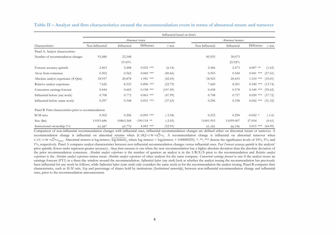
We find that 19.4% of the recommendation changes for the whole sample are influential

in terms of abnormal return and 25.9% in abnormal turnover. While only 10.6% of the

recommendation changes are influential on both. In contrast, Loh and Stulz (2011) find that

11.7% and 12.8% of recommendation revisions are influential in terms of abnormal return and

turnover respectively. Further, we see that our results are higher between 2003 and 2012 (21.9%

and 28.8%) but lower before 2003 (16.5% and 22.5%), which indicates that Reg_FD act had a

positive impact on analyst recommendations.

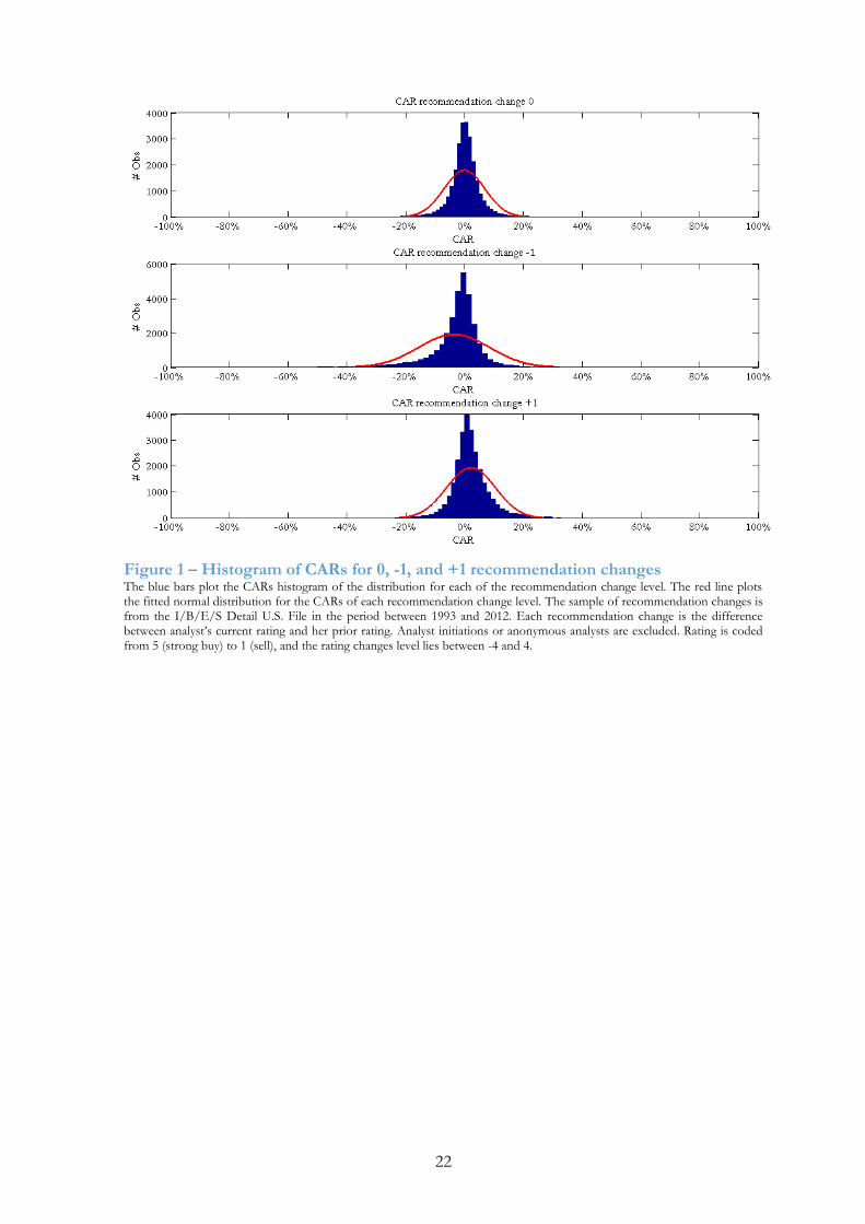
Figure 1 plots the two-day CAR histogram of recommendation changes for zero-point

and one-point magnitude changes, as these categories include about 75% of the total

recommendation changes. The top chart plots the histogram for CARs of the no

recommendation change category, which mostly fall close to zero. The charts below plot the

histograms for the one-point downgrade and upgrade, which are negatively and positively

skewed respectively. This shows that the direction of the recommendation change indicates the

sign of the return obtained during the first two days after issuing the recommendation.

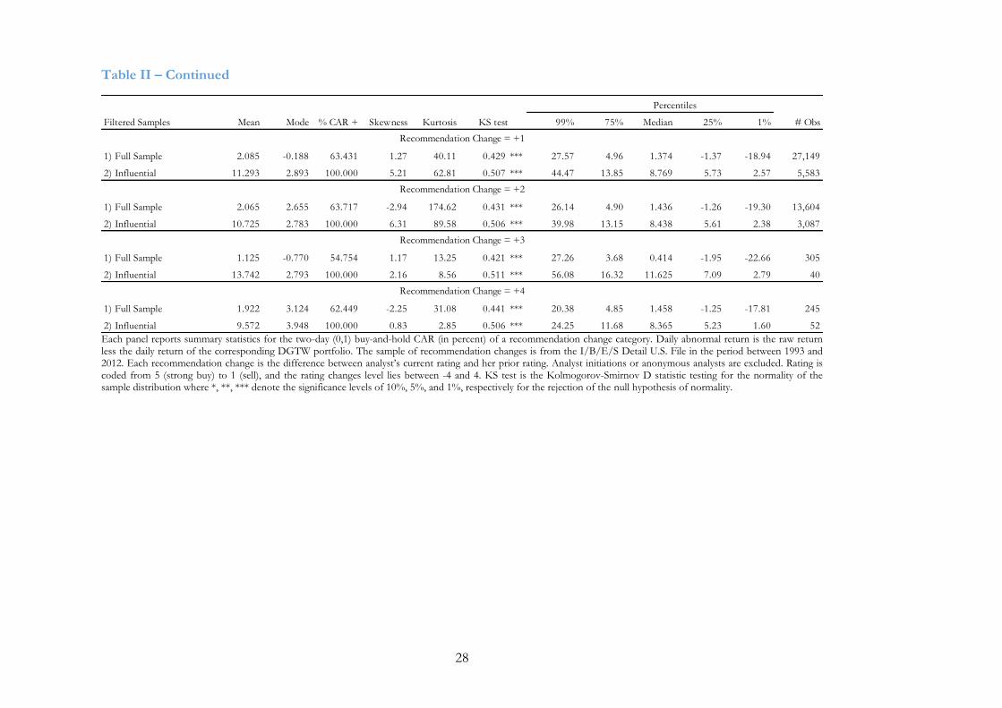
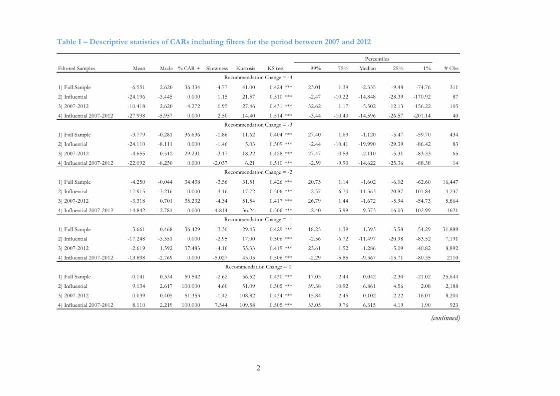
Table II reports the descriptive statistics of CARs for our sample of recommendation

changes, grouped by the recommendation change categories from -4 to +4. All positive

(negative) rating changes categories have positive (negative) CAR means and medians. For

negative revisions the 25th and 1st percentiles have larger negative returns opposed to the positive

ones. This shows that company specific news-recommendations and outliers have a strong

impact on the means. Filtering the CAR means for influential recommendation changes we

7

notice that these have changed and are more distant from zero but still follow the same pattern

compared to the whole sample. Regarding the 1st percentile for the positive (negative)

recommendation change categories the CARs are all above (below) zero. These results describe

how the tails of the results look like and show the statistical and economic significance of

influential recommendations. Investors, who are able to successfully identify these

recommendations changes when they are issued, are able to profit from significant returns.

3. Predicting influential recommendations

In this section we look at the determinants of influential recommendation changes. First we

define the characteristics specific characteristics of analyst, which have been shown to have an

impact on the stock price when a recommendation is issued. Then we look at how

recommendation, analyst, and firm characteristics vary between influential recommendation

changes and all recommendation changes. Also, we study the likelihood that a certain

characteristic will result in an influential recommendation change.

3.1. The determinants

Earnings forecast accuracy: Loh and Mian (2006) show that analysts who more

accurately forecast earnings also issue more profitable stock recommendations and therefore

such analysts can have a larger impact on the stock price. We compute the Earnings forecast

accuracy quintile of an analyst by sorting analysts within a firm-year into quintiles using the last

unrevised FY1 forecast of the analyst, as proposed by Loh and Stulz (2011). The forecast

accuracy rank (1 being the most accurate) is assigned to the analyst for the recommendations that

the analyst issues during the 12-month window that overlaps three months into the next fiscal

year, following Loh and Mian (2006). This allows to apply the accuracy rank during the months

when the fiscal year’s actual earnings are announced.

8

Away from consensus: Jegadeesh and Kim (2010) analyze if analysts have a tendency to

take similar actions around the same time. To understand whether an analyst is not affected by

this bias, implying that he is away from the consensus, we test if the deviation of a new

recommendation is greater than the prior absolute deviation of the recommendation consensus,

as suggested by Loh and Stulz (2011).

Analyst experience: According to Mikhail, Walther, and Willis (1997) earnings forecast

accuracy of analysts improve with experience. Thus, experience can be associated to the impact

of influential recommendation changes. We measure analyst experience measured as the number

of quarters since the analyst issued the stock recommendation on I/B/E/S. Loh and Stulz

(2011) suggest to analyze analyst experience in both absolute and relative terms. Absolute analyst

experience represents the total number of quarters that analyst appeared on I/B/E/S. While

Relative analyst experience is the numbers of quarters the analyst has covered that specific firm

minus the average experience for all analysts covering the firm.

Concurrent Earnings Forecast: Stock recommendations supplemented by earnings

forecast revisions have greater price movements (Kecskes, Michaely, and Womack, 2009).

Hence, we include a Concurrent earnings forecast indicator variable specifying if the same analyst

issued a FY1 forecast in the three-day window around the recommendation revision.

Influential Before: Loh and Stulz (2011) show that a recommendation change by an

analyst, who has previously been influential for any stock increases the likelihood of an

influential recommendation change. The likelihood further increases if the analyst had already

been influential for the same stock. Therefore, we look at both analysts that had previously been

influential for any stock and the same stock.

3.2. Influential versus non-influential recommendation changes

To understand the determinants of influential recommendation we analyze in table III the

differences of the characteristics between regular analyst recommendations revisions and

9

influential. While in table IV, using an in sample Probit estimation, we look at what

characteristics increase the predictability of an analyst recommendation change.

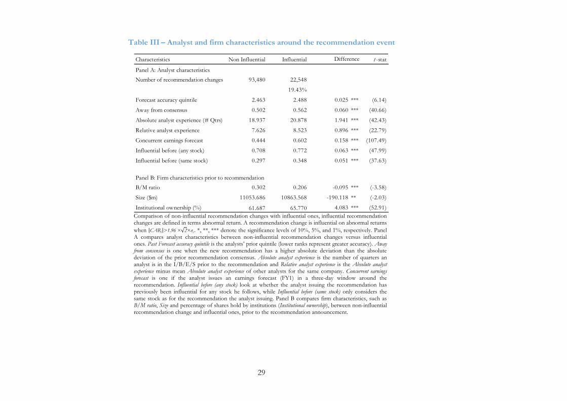
In Table III, we observe that influential recommendations revisions are less accurate, in

terms of earnings forecasts, than non-influential recommendation revisions, as the 1st quintile

represents the most accurate analysts. This finding is inconsistent with Loh and Mian (2006)

result that more accurate earnings forecasts generate greater annual returns. From Table IV,

earnings forecast accuracy does not provide much incremental predictability. We find that, on

average, influential recommendation changes are further Away from consensus (Table III). In line

with Jegadeesh and Kim (2010), we find that recommendation changes that are further Away from

consensus are more likely to be influential (Table IV). In alignment with Mikhail, Walther, and

Willis (1997), we find that analysts, who issue influential recommendation changes, have more

experience but do not necessarily increase the predictive power of an influential

recommendation. Kecskes, Michaely and Womack (2012) find that recommendations

accompanied by earnings forecast revisions have larger price reactions. In line with their findings

we observe in Table III that more than 60% of the influential recommendations were issued by

analysts, who issued an earnings forecast between a three-day window around the

recommendation announcement. Moreover, it also significantly increases the predictability of an

influential recommendation (Table IV). Table IV shows that analysts, who have previously been

influential for any of the stocks they follow, are more likely to produce an influential

recommendation. But analysts, who issue a recommendation for a firm for which they have been

influential before, have less probability of issuing an influential recommendation change

In line with Stickel (1995), who finds that the stock-price reaction for smaller firms is

greater than for larger ones, the difference in size does not change significantly for influential

recommendations (Table III). Nevertheless, Table IV shows that recommendation changes for

large firms have a negative marginal effect, meaning that small firms increase the predictability of

an influential recommendation change. In terms of book-to-market we observe, both in Table

10

III and IV that growth firms have an incremental impact on the predictability of an influential

recommendation change, opposed to value firms. Comparing recommendation changes on firms

related to the financial and insurance sector, we see that these are less likely to be influential

(Table IV). We find that influential recommendations are associated with higher institutional

ownership firms. This is consistent with Kelsey et al. (2007) findings that analysts, who follow

firms with higher institutional ownership, issue more accurate earnings forecast and also react

faster to new information.

In Table IV, we observe that recommendation level does not increase the probability of

issuing an influential recommendation change. An explanation for this is related to the fact that

the recommendation level itself does not contain information about the past performance

relative to the future expectations of the stock. In line with Asquith, Au and Mikhail (2005)

finding that the content of recommendation has an impact, as recommendations with larger

magnitudes should include more new information. The absolute recommendation change value

shows a strong impact on the likelihood of issuing an influential recommendation change.

Meaning that when a recommendation moves from sell (strong buy) to strong buy (sell), equal to

a four-point magnitude upgrade (downgrade), a recommendation change is more likely to be

influential (the bottom chart in Figure 2 plots the transition probabilities of the influential

recommendation changes). Consistent with Loh and Stulz (2011), we find evidence that the

Regulation Fair Disclosure act from 2000, Reg_FD, has a significant marginal effect in the

predictability of an influential recommendation. This shows that through the regulatory change

investors started to give more attention to analyst recommendations.

3.3. Forecast

To forecast influential recommendation changes for an out of sample investment strategy, we

run, on monthly basis, a Probit regression with a five-years rolling window. The first estimation

is between January 1994 and December 1998. This way we are able to account for changes in the

11

marginal effect of the characteristics to predict influential recommendation changes for the

following month.

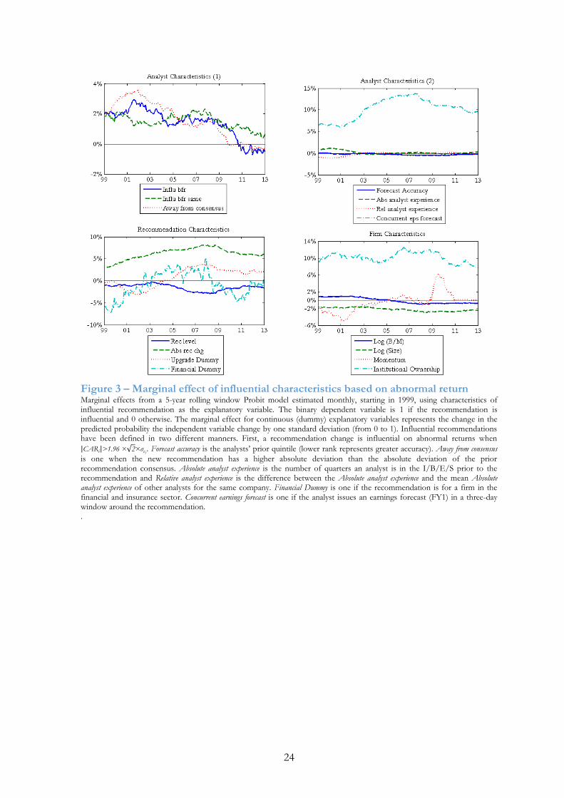
Looking at Figure 3 we observe that Absolute value of recommendation change, Concurrent

earnings forecast, and Institutional ownership are the main characteristics used in this strategy to

predict influential recommendation changes. The greater the value of the absolute

recommendation change the more likely it is that the recommendation change will be influential.

We would expect this as a greater magnitude means that the analyst has come to conclusions

regarding the firm, which have significantly changed his opinion concerning the prospects of the

firm. A concurrent earnings forecast means that the analyst has not only considered how the

firm will perform compared to its peers but also performed a deeper analysis, which led him to

issue a new earnings forecast. To predict influential recommendation for the strategy we only

consider earnings forecasts issued between t-3 and t, opposed to t-3 to t 3 used for the ex post

analysis of influential recommendation changes. Moreover, the fact that institutional ownership is

also a key characteristic shows that institutional investors are more concerned with the opinion

of sell-side analysts. One possible explanation for this is that analysts primarily target their

recommendation to institutional investors and also spend more time giving them a detailed

explanation of their analysis.

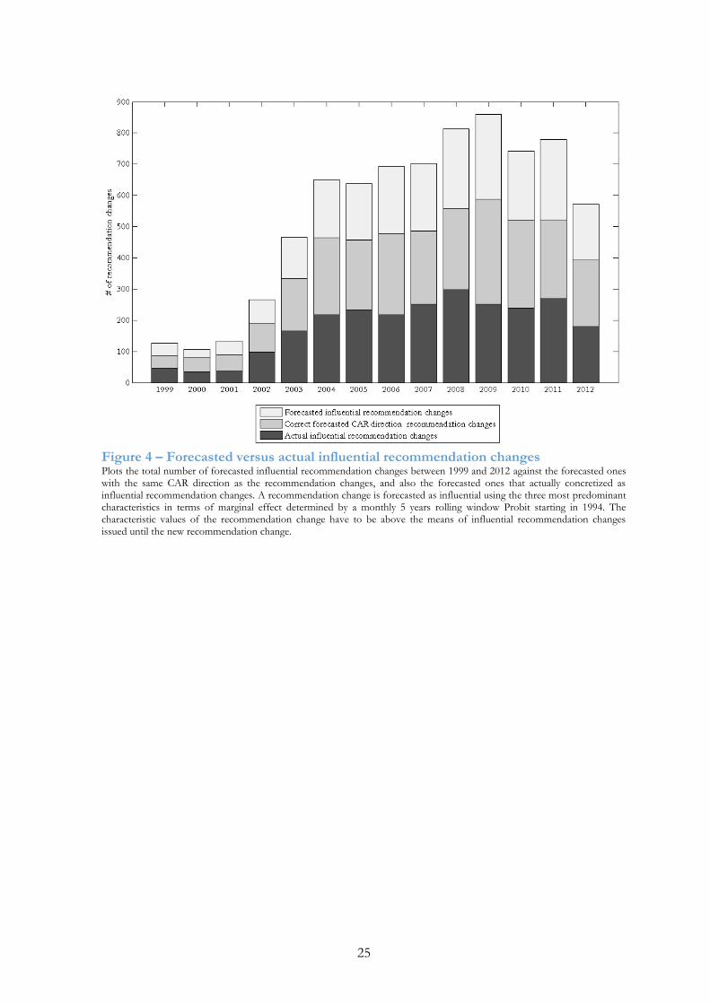
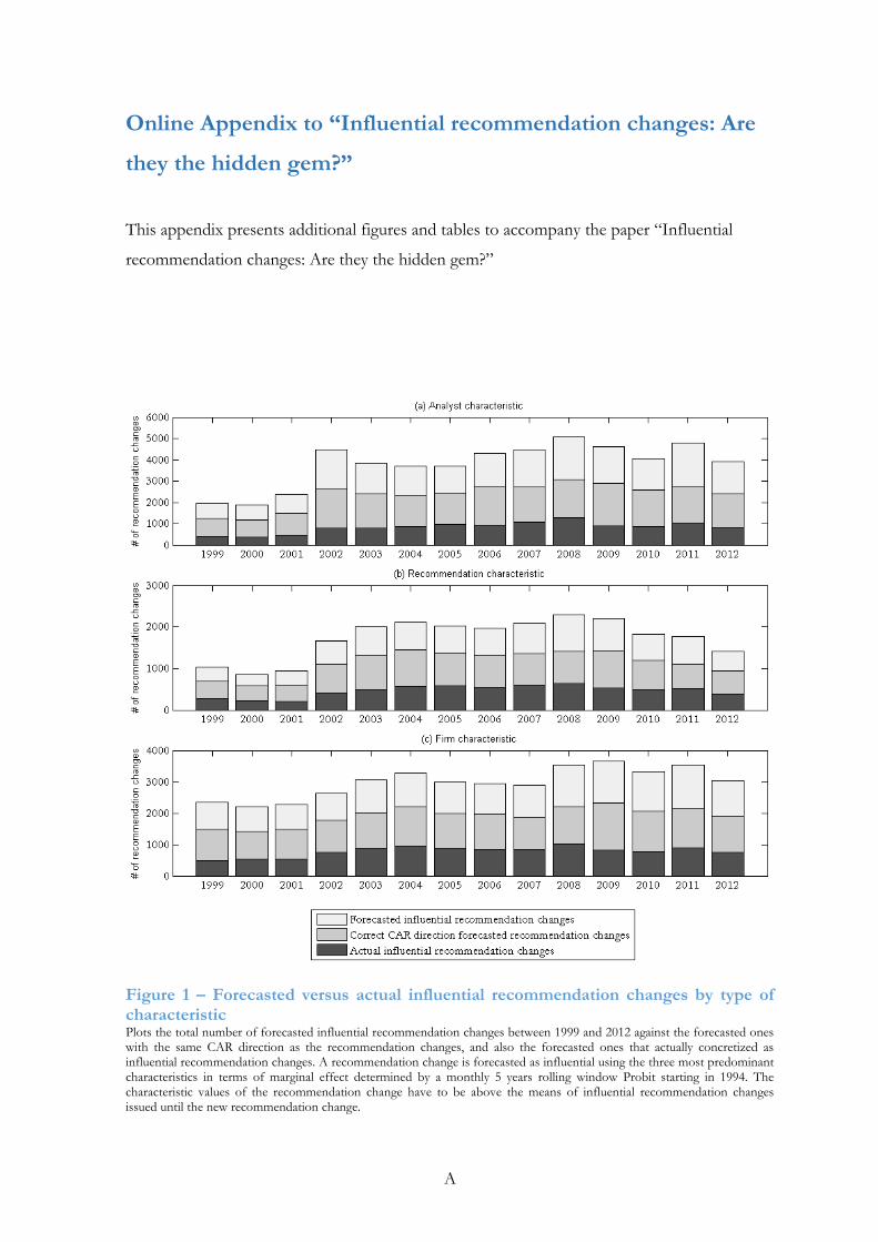
We perform an analysis of how well the three most predominant characteristics, absolute

recommendation change, concurrent earnings forecast, and institutional ownership can predict influential

recommendation changes. To predict an influential recommendation change we define the

critical value, on monthly basis, by looking at the mean value of the characteristic for influential

recommendation changes between the starting period of our sample and the prior month. If the

characteristic is above the critical value when the recommendation change is issued we forecast it

to be an influential recommendation change. Using only the absolute recommendation change

characteristic we are able correctly identify 26.6%, by the means of the concurrent earnings forecast

characteristic 26.3%, and using institutional ownership characteristic a mere 21.7%. However, by

12

combining the three characteristics we are able to accurately predict 33.6% influential

recommendation changes. Figure 4 shows the evolution of the forecasted influential

recommendation changes using the combination of the three recommendation characteristics

against the recommendation changes that actually realized as influential between 1999 and 2012.

4. Investment strategy

Previous literature has shown that by using analyst recommendations for investment strategies,

one is able to create significant alphas. Barber et al. (2001) find that an investment strategy based

on average recommendations of analysts, long (short) on the buy (sell) recommendations, yields

annualized returns of 18.8% (5.8%) between 1986 and 1996 in the US. Other literature has

shown that strategies based on average analyst recommendation revisions have more impact than

merely on average analyst recommendations. Green (2006) finds that a strategy tracking

recommendation revisions results in an average two-day return of 1.0% (1.5%) for upgrades

(downgrades) after transaction costs. Barber, Lehavy and Trueman (2010) find that a strategy

conditioned on recommendation levels (changes) yields an annualized abnormal return of 8.8%

(9.6%). By creating a new strategy that is conditioned on both recommendation levels and

changes they achieve an annualized return improvement of 3.5%.

Our objective is to create an out of sample investment strategy that is based on

forecasting influential recommendation changes. To be able to forecast influential

recommendation changes, we estimate, on a monthly basis, the marginal effects of

recommendation revisions characteristics using a 5 year rolling window Probit regression. Each

month we identify three characteristics, (one recommendation characteristic, one analyst

characteristic and another related to the firm) with the highest marginal effect. To identify

whether the recommendation change will be influential we compare the characteristics to the

mean of previous influential recommendations. On the recommendation announcement date the

characteristics have to be greater than the means to be include in the corresponding long or

13

short portfolio. The position is than held for a period of one month. Additionally, we compare

our results with other investment strategies that consider analyst recommendations.

4.1. Buying/selling influential recommendation changes

We compare our results with the CRSP equally-weighted index (Panel A of Table V).

Additionally, we construct a 1/N portfolio of our entire sample (Panel B), as it has been found

that it performs as well as other portfolio allocation strategies in an out of sample analysis

(DeMiguel, Garlappi and Uppal, 2009). We exclude the stock if the price on the

recommendation announcement date (t ) is below $5. As D’Avolio (2002) shows that it is hard

to borrow stocks with a price below $5, and therefore these stocks are not suitable for strategies

that involve short-selling.

Panel C shows how the first investment approach (i) with all recommendation changes

performs, while the strategy in Panel D consists only of recommendation changes that are

predicted to be influential. Table V shows that the investment approach (i) yields the best result.

The two long-short portfolios in Panel C and D have a Sharpe ratio of 0.59 and 1.22 and an

annualized CEQ return of 27.7% and 10.7%. Both of these strategies over-perform compared to

our benchmarks, the CRSP equally-weighted index has a Sharpe ratio of 0.40 and annualized

CEQ of 6.2%, while the naïve strategy has a Sharpe ratio of 0.26 and an annualized CEQ of

3.7%.

4.2. Comparison with other analyst recommendations strategies

Several strategies that consider analyst recommendations have previously been studied and show

positive results. That is why we want to understand how our proposed strategy, in section 4.1.,

compares to these other strategies. Our first benchmark investment approach is based on Barber

et al. (2001) and uses a recommendation consensus of the last six months. We compare this

approaches into two different kinds of strategies, one that considers all recommendations and

14

one that is only concerned by influential recommendations. The first strategy uses all

recommendations to build the consensus, and the second one only considers recommendations

that were influential. We observe that the long-short portfolio that is conditioned to influential

recommendation changes performs worse, annualized Sharpe ratio of -0.09 and CEQ of -1.1%,

than its counterparty that includes all recommendation, annualized Sharpe ratio of -0.17 and

CEQ of 0.2%. Hence, an investor following a strategy that is based on consensus

recommendation levels will have a worse performance when compared to our proposed strategy

of buying /selling influential recommendation changes and the CRSP equally-weighted index.

The second benchmark investment approach considers a consensus constructed on

recommendation changes and not levels, as proposed by Green (2006). Similarly, we build two

strategies, where the first one includes all recommendations and the second only uses influential

recommendation changes for the consensus. By using a consensus that considers the

recommendation changes and not the level, we note that the long-short portfolio, which

considers all recommendation changes, improves compared to the portfolio in that is based on

recommendation level, the annualized Sharpe ratio increases by 0.20 and the CEQ by 2.0%.

However, the long-short portfolio, which only takes influential recommendation changes into

account, has a poorer performance compared to its counterparty. The annualized Sharpe ratio

decreases by 0.40 and the CEQ by 2.7%. Likewise, to the previous benchmark we find that the

CRSP equally weighted index and our proposed strategy that is conditional to predicted

influential recommendation changes perform significantly better.

4.3. Strategy implementation

To implement our proposed strategy an investor only needs to define the characteristics of

analyst recommendations, as we do in section 3. Then by running a Probit regression of a

monthly basis she can establish the three most relevant recommendation change characteristics.

15

With this information the investor is then able to determine when a recommendation change is

issued whether it is likely that this one will be influential.

Example: Analyst J. Doe issues a recommendation for stock XYZ with a strong buy

rating. The previous outstanding recommendation by J. Doe for stock XYZ was a hold. The

portfolio manager ran the Probit regression at the beginning of the month to define which three

characteristics are important for this month. She identified Absolute value change, Concurrent earnings

forecast, and Institutional Ownership as the ones with the most predictive power. Additionally, she

knows what the average value of these characteristics for influential recommendation is, 1.5 for

Absolute value change, 80% for Concurrent earnings forecast, and 65% for Institutional Ownership. With

this information she can now examine the new recommendation change. She identifies that the

recommendation change moved by two levels, which is greater than the average of 1.5. Also, that

the analyst issued a new earnings forecast the day before, 80% of Concurrent earnings forecast means

that the presence of an earnings forecast is important. Last, the percentage of institutional

ownership for this stock is 67%. The portfolio manager concludes that all characteristics are

above the average value and the recommendation change direction is positive. Consequently, she

concludes that a buy position for this XZY should be added to her portfolio. If any of the

characteristics would not have been in line with the average value of the influential

recommendation change characteristics, the analyst would have disregarded this

recommendation.

5. Robustness checks

As mentioned in section 4 there are several steps involved in forming the different strategies.

Thus, we examine whether the performance of the main strategy, which predicts influential

recommendation changes and buys or sell stock accordingly, still dominates when we modify

some of the steps involved in the process. First, period of time; Second, holding period; Third;

TPER; Finally, we consider how transaction costs affect the different strategies.

16

5.1. Period of time

As the results of our strategy may be driven by the selected time period, we run the same analysis

for different periods. The first period starts in 2003. We observe that the annualized Sharpe ratio

decreases to 1.03. While in the second period, which starts in 2008, annualized Sharpe ratio has a

stronger reduction to 0.50. During these two periods, the CRSP equally-weighted index has a

poorer performance compared to both of these strategies, a Sharpe ratio of 0.48 and 0.26 for the

first sub period and the second sub period respectively.

5.2. Holding period

It is possible that the results in the third investment approach (iii) that buys recommendation

changes are driven by the holding period. We change this assumption to one quarter (63 trading

days). In line with Stickel (1995), we observe a reduction in annualized mean returns, more

importantly both long portfolios have negative Sharpe ratios. However, the long-short portfolio

still has positive Sharpe ratio of 0.58. Compared to the CRSP equally-weighted index, which has

a Sharpe ratio of 0.40, the strategy using all recommendation changes becomes unattractive.

Therefore, we see that increasing the holding period has a negative impact on the strategy’s

result, especially for an investor who is considering all recommendation changes and is

constrained to long-only investments.

5.3. Target price expected return

Additionally, we consider how changes in TPER consensus can be used in conjunction with our

stock recommendation strategies. According to Brav and Lehavy (2 3) analysts’ target price

contain incremental information, as there is a significant market reaction to target price revisions.

Further, Asquith, Au and Mikhail (2005) find that target price revisions hold new information

even in the company of stock recommendation change and earnings revisions. Huang, Mian and

Sankaraguruswamy (2 9) find that by combining analysts’ target price revisions and consensus

17

recommendation, they are able to improve the returns and reduce risk exposure, compared to

implementing analysts’ target price revisions and consensus recommendations portfolios

separately. Thus, we also analyze the performance of the combination of the consensus

approaches with change in consensus target price.

To construct the long portfolio and the short portfolio we rank the changes in TPER

consensus into three. The long portfolio includes all stocks that have the highest changes in

TPER consensus, while the short portfolio contains all the stocks that have the lowest changes

in TPER consensus. Our results show that the long portfolio has an annualized Sharpe ratio of -

0.68 and a CEQ 0.6%, which is similar to the naïve strategy. However, both the short and long-

short portfolios have a poorer performance compared to our proposed approach which predicts

influential recommendation changes. We also look at how changes in TPER recommendation

consensus can be combined with recommendation consensus, investment approach (ii), or

recommendation changes consensus, investment approach (iii), considering all recommendations

and only influential ones. We find that the new long portfolios for these two strategy approaches

improve, while the results for the short portfolios deteriorate. This leads to new long-short

portfolios, which have similar results as the portfolios that did not consider changes in TPER

recommendation consensus and have poorer performance compared to the (i) investment

approach that forecasts influential recommendation changes.

5.4. Transaction costs

To incorporate trading costs (i.e. bid-ask spread, brokerage commissions, trading impact) we

estimate the annualized turnover, as in Barber et al. (2001). For each stock i in portfolio p, we

calculate at the close of the trading date on t-1 the new fraction of weights of the portfolio at the

close of the trading date t, assuming that there was no portfolio rebalancing (G

- - -

(8)

18

Secondly, F , which represents the actual fraction of stock i in portfolio p, on date t

taking into account any portfolio rebalancing, is subtracted from G . The turnover for firm i at

time t is given by

max -

(9)

The annual turnover is calculated by multiplying by the number of months (trading days)

in a year with . Table V shows that most long-short strategies have an annual turnover close

to 100%. This means that over a period of one year the portfolio fully rotates. As expected, the

two long-short portfolios in Panel G and H have significantly higher turnover, 479.8% and

412.7% respectively. Using the annual turnover we proxy transaction costs by means of the

round-trip cost of the bid-ask spread estimated to be 1% [e.g. individual investors (Barber and

Odean, 2000), and mutual funds (Carhart 1997)]. Looking at Table V we observe that the

minimum annual transaction cost would reduce the annualized abnormal return of the long-

short portfolio, which is based on all recommendations, to 15.4% (4.8% reduction), of the long-

short portfolio, which acts on predicted influential recommendations, to 27.4% (4.1%

reduction), and of the naïve strategy to 6.6% (0.6% reduction). This indicates that even after

transaction costs the long-short portfolio conditioned to predicted influential recommendations

is still a valuable strategy.

6. Conclusion

Stock analysts sell themselves to clients as experts since they are able to bring new and valuable

information to them. The press has reported on several cases where stock analysts had a

significant impact with their recommendation change on stock returns (e.g. AIG). Most literature

is concentrated on the average market price reaction of stock recommendation changes.

Following Loh and Stulz (2011), we find that approximately 20% of the recommendation

changes are influential in terms of abnormal return.

19

Using the three most predominant characteristics of influential recommendation

revisions, Absolute recommendation change value, prior Concurrent earnings forecast, and Institutional

ownership percentage, we construct a long-short portfolio that predicts influential recommendation

changes and buys positive and sells negative ones from 1999 to 2012. This portfolio yields a net

annualized abnormal return of 27.4% using the four factor model, a Sharpe ratio of 1.22, and a

CEQ return of 27.7%. Compared to the CRSP equally-weighted index, which has a Sharpe Ratio

of 0.40 and an annualized CEQ return of 6.2%, during the same period we find that our

proposed strategy, which influential recommendation changes based on the three most

predominant characteristics.

To conclude, we show that some recommendation changes have a greater impact on the

market and that by creating a strategy based on these characteristics we achieve to construct a

portfolio that has significantly better performance, compared to other strategies that have been

previously studied.

References

Altinkilic, Oya, and Robert S. Hansen, 2009, On the Information Role of Stock

Recommendation Revisions, Journal of Accounting and Economics 48, 17-36.

Asquith, Paul, Andrea S. Au, and Michael B. Mikhail, 2005, Information Content of Equity

Analyst Reports, Journal of Financial Economics 75, 245-282.

Barber, Brad M., Reuven Lehavy, Maureen McNichols, and Brett Trueman, 2001, Can Investors

profit from the prophets? Security analyst recommendations and stock returns, The

Journal of Finance 56, 531 - 563.

Barber, Brad M., Reuven Lehavy, and Brett Trueman, 2010, Ratings Changes, Ratings Levels,

and the Predictive Value of Analysts’ Recommendations, Financial Management 39, 533-

553.

Barber, Brad M., and Terrance Odean, 2000, Trading Is Hazardous to Your Wealth: The

Common Stock Investment Performance of Individual Investors, The Journal of Finance

55, 773-806.

20

Boni, Leslie, and Kent L. Womack, 2006, Analysts, Industries, and Price Momentum. The Journal

of Financial and Quantitative Analysis 41, 85-109.

Brav, Alon, and Reuven Lehavy, 2003, An Empirical Analysis of Analysts' Target Prices: Short-

term Informativeness and Long-term Dynamics, The Journal of Finance 58, 1933-1986.

Carhart, Mark M., 1997, On Persistence in Mutual Fund Performance, The Journal of Finance 52,

57-82.

Daniel K., M. Grinblatt, S. Titman, R. Wermers, 1997, Measuring Mutual Fund Performance

with Characteristic-based Benchmarks, The Journal of Finance 52, 153-193.

D’Avolio, Gene, 2002, The Market for Borrowing Stock, Journal of Financial Economics 66, 271–

306.

DeMiguel, Victor, Lorenzo Garlappi, and Raman Uppal, 2009, Optimal Versus Naive

Diversification: How efficient is the 1/N Strategy?, The Review of Financial Studies 22,

1915-1953.

Frankel, Richard, S.P. Kothari, and Joseph Weber, 2006, Determinants of the Informativeness of

Analyst Research, Journal of Accounting and Economics 41, 29-54.

Green, T. Clifton, 2006, The Value of Client Access to Analyst Recommendations, Journal of

Financial and Quantitative Analysis 41, 1-24.

Huang, Joshua, G. Mujtaba Mian, and Srinivasan Sankaraguruswamy, 2009, The Value of

Combining the Information Content of Analyst Recommendations and the Target

Prices, Journal of Financial Markets 12, 754-777.

Ivkovic, Zoran, and Narasimhan Jegadeesh, 2004, The Timing and Value of Forecast and

Recommendation Revisions, Journal of Financial Economics 73, 433-463.

Jegadeesh, Narasimhan, and Sheridan Titman, 1993, Returns to Buying Winners and Selling

Loosers: Implications for Stock Market Efficiency, The Journal of Finance 48, 65-91.

Jegadeesh, Narasimhan, and Woojin Kim, 2010, Do Analysts Herd? An Analysis of

Recommendations and Market Reactions, The Review of Financial Studies 23, 901-937.

Kecskes, Ambrus, Roni Michaely, and Kent L. Womack, 2010, What Drives the Value of

Analyst's Recommendations: Earnings Estimates or Discount Rate Estimates?, Working

Paper, Darthmouth College.

21

Kelsey, D. Wei, Alexander Ljungqvist, Felicia Marston, Laura T. Starks, and Hong Yan, 2007,

Conflicts of Interest in Sell-side Research and the Moderating Role of Institutional

Investors, Journal of Financial Economics 85, 420-456.

Ljungqvist, Alexander, Christopher Malloy, and Felicia Marston, 2009, Rewriting History, The

Journal of Finance 64, 1935-1960.

Llorente, Guillermo, Roni Michaely, Gideon Saar, and Jiang Wang, 2002, Dynamic

Volume‐Return Relation of Individual Stocks, The Review of Financial Studies 15, 1005-

1047.

Loh, Roger K., and G. Mujtaba Mian, 2006, Do Accurate Earnings Forecasts Facilitate Superior

Investment Recommendations?, Journal of Financial Economics 80, 455-483.

Loh, Roger K., and René M. Stulz, 2011, When Are Analyst Recommendation Changes

Influential?, The Review of Financial Studies 24, 593-627.

Mikhail, Michael B., Beverly R. Walther, and Richard H. Willis, 1997, Do Security Analysts

Improve Their Performance with Experience?, Journal of Accounting Research 35, 131-157

Stickel, Scott.E, 1995, The Anatomy of Buy and Sell Recommendations, Financial Analyst Journal

51, 25-39.

Womack, Kent L, 1996, Do Brokerage Analysts' Recommendations Have Investment Value?,

The Journal of Finance 51, 137-167.

22

Figure 1 – Histogram of CARs for 0, -1, and +1 recommendation changes The blue bars plot the CARs histogram of the distribution for each of the recommendation change level. The red line plots the fitted normal distribution for the CARs of each recommendation change level. The sample of recommendation changes is from the I/B/E/S Detail U.S. File in the period between 1993 and 2012. Each recommendation change is the difference between analyst’s current rating and her prior rating. Analyst initiations or anonymous analysts are excluded. Rating is coded from 5 (strong buy) to 1 (sell), and the rating changes level lies between -4 and 4.

23

Figure 2 – Transition probabilities of recommendation changes This chart plots the transition probabilities of recommendation changes, meaning the probability that a prior recommendation transits to any of the five rating classifications. The top chart plots the transition probabilities of the whole sample and the bottom chart the transition probabilities of influential recommendation changes. The sample of recommendation changes is from the I/B/E/S Detail U.S. File in the period between 1993 and 2012. Each recommendation change is the difference between analyst’s current rating and her prior rating. Analyst initiations or anonymous analysts are excluded. Rating is coded from 5 (strong buy) to 1 (sell), and the rating changes level lies between -4 and 4.

24

Figure 3 – Marginal effect of influential characteristics based on abnormal return Marginal effects from a 5-year rolling window Probit model estimated monthly, starting in 1999, using characteristics of influential recommendation as the explanatory variable. The binary dependent variable is 1 if the recommendation is influential and 0 otherwise. The marginal effect for continuous (dummy) explanatory variables represents the change in the predicted probability the independent variable change by one standard deviation (from 0 to 1). Influential recommendations have been defined in two different manners. First, a recommendation change is influential on abnormal returns when

. Forecast accuracy is the analysts’ prior quintile (lower rank represents greater accuracy). Away from consensus

is one when the new recommendation has a higher absolute deviation than the absolute deviation of the prior recommendation consensus. Absolute analyst experience is the number of quarters an analyst is in the I/B/E/S prior to the recommendation and Relative analyst experience is the difference between the Absolute analyst experience and the mean Absolute analyst experience of other analysts for the same company. Financial Dummy is one if the recommendation is for a firm in the financial and insurance sector. Concurrent earnings forecast is one if the analyst issues an earnings forecast (FY1) in a three-day window around the recommendation. .

25

Figure 4 – Forecasted versus actual influential recommendation changes Plots the total number of forecasted influential recommendation changes between 1999 and 2012 against the forecasted ones with the same CAR direction as the recommendation changes, and also the forecasted ones that actually concretized as influential recommendation changes. A recommendation change is forecasted as influential using the three most predominant characteristics in terms of marginal effect determined by a monthly 5 years rolling window Probit starting in 1994. The characteristic values of the recommendation change have to be above the means of influential recommendation changes issued until the new recommendation change.

26

Table I – Transition probabilities of recommendation changes

Reports the transition probabilities of recommendations changes (e.g. in column 5 when the prior recommendation is a sell, it has a probability of 8.9% of moving to a strong buy in the next quarter). The sample of recommendation changes is from the I/B/E/S Detail U.S. File in the period between 1993 and 2012. Each recommendation change is the difference between analyst’s current rating and her prior rating. Analyst initiations or anonymous analysts are excluded. Rating is coded from 5 (strong buy) to 1 (sell), and the rating changes level lies between -4 and 4.

Current Recommendation

1 2 3 4 5

(Sell) (Underperform) (Hold) (Buy) (Strong Buy) Total

1 (Sell) 241 194 2,120 166 245 2,966

8.1% 6.5% 71.5% 5.6% 8.3% 100%

2 (Underperform) 239 1,073 3,761 632 139 5,844

4.1% 18.4% 64.4% 10.8% 2.4% 100%

3 (Hold) 2,226 4,193 11,206 14,775 10,852 43,252

5.1% 9.7% 25.9% 34.2% 25.1% 100%

4 (Buy) 226 793 18,397 8,299 8,419 36,134

0.6% 2.2% 50.9% 23.0% 23.3% 100%

5 (Strong Buy) 311 208 13,428 9,060 4,825 27,832

1.1% 0.7% 48.2% 32.6% 17.3% 100%

Total 3,243 6,461 48,912 32,932 24,480 116,028

Prior Recommendation

27

Table II – Descriptive statistics of CARs

(continued)

Percentiles

Filtered Samples Mean Mode % CAR + Skewness Kurtosis KS test 99% 75% Median 25% 1% # Obs

Recommendation Change = -4

1) Full Sample -6.551 2.620 36.334 -4.77 41.00 0.424 *** 23.01 1.39 -2.335 -9.48 -74.76 311

2) Influential -24.196 -3.445 0.000 1.15 21.57 0.510 *** -2.47 -10.22 -14.848 -28.39 -170.92 87

Recommendation Change = -3

1) Full Sample -3.779 -0.281 36.636 -1.86 11.62 0.404 *** 27.40 1.69 -1.120 -5.47 -59.70 434

2) Influential -24.110 -8.111 0.000 -1.46 5.03 0.509 *** -2.44 -10.41 -19.990 -29.39 -86.42 83

Recommendation Change = -2

1) Full Sample -4.250 -0.044 34.438 -3.56 31.51 0.426 *** 20.73 1.14 -1.602 -6.02 -62.60 16,447

2) Influential -17.915 -3.216 0.000 -3.16 17.72 0.506 *** -2.57 -6.70 -11.363 -20.87 -101.84 4,237

Recommendation Change = -1

1) Full Sample -3.661 -0.468 36.429 -3.30 29.45 0.429 *** 18.25 1.39 -1.393 -5.58 -54.29 31,889

2) Influential -17.248 -3.351 0.000 -2.95 17.00 0.506 *** -2.56 -6.72 -11.497 -20.98 -83.52 7,191

Recommendation Change = 0

1) Full Sample -0.141 0.334 50.542 -2.62 56.52 0.430 *** 17.03 2.44 0.042 -2.30 -21.02 25,644

2) Influential 9.134 2.617 100.000 4.60 51.09 0.505 *** 39.38 10.92 6.861 4.56 2.08 2,188

28

Table II – Continued

Each panel reports summary statistics for the two-day (0,1) buy-and-hold CAR (in percent) of a recommendation change category. Daily abnormal return is the raw return less the daily return of the corresponding DGTW portfolio. The sample of recommendation changes is from the I/B/E/S Detail U.S. File in the period between 1993 and 2012. Each recommendation change is the difference between analyst’s current rating and her prior rating. Analyst initiations or anonymous analysts are excluded. Rating is coded from 5 (strong buy) to 1 (sell), and the rating changes level lies between -4 and 4. KS test is the Kolmogorov-Smirnov D statistic testing for the normality of the sample distribution where *, **, *** denote the significance levels of 10%, 5%, and 1%, respectively for the rejection of the null hypothesis of normality.

Percentiles

Filtered Samples Mean Mode % CAR + Skewness Kurtosis KS test 99% 75% Median 25% 1% # Obs

Recommendation Change = +1

1) Full Sample 2.085 -0.188 63.431 1.27 40.11 0.429 *** 27.57 4.96 1.374 -1.37 -18.94 27,149

2) Influential 11.293 2.893 100.000 5.21 62.81 0.507 *** 44.47 13.85 8.769 5.73 2.57 5,583

Recommendation Change = +2

1) Full Sample 2.065 2.655 63.717 -2.94 174.62 0.431 *** 26.14 4.90 1.436 -1.26 -19.30 13,604

2) Influential 10.725 2.783 100.000 6.31 89.58 0.506 *** 39.98 13.15 8.438 5.61 2.38 3,087

Recommendation Change = +3

1) Full Sample 1.125 -0.770 54.754 1.17 13.25 0.421 *** 27.26 3.68 0.414 -1.95 -22.66 305

2) Influential 13.742 2.793 100.000 2.16 8.56 0.511 *** 56.08 16.32 11.625 7.09 2.79 40

Recommendation Change = +4

1) Full Sample 1.922 3.124 62.449 -2.25 31.08 0.441 *** 20.38 4.85 1.458 -1.25 -17.81 245

2) Influential 9.572 3.948 100.000 0.83 2.85 0.506 *** 24.25 11.68 8.365 5.23 1.60 52

29

Table III – Analyst and firm characteristics around the recommendation event

Comparison of non-influential recommendation changes with influential ones, influential recommendation changes are defined in terms abnormal return. A recommendation change is influential on abnormal returns

when . *, **, *** denote the significance levels of 10%, 5%, and 1%, respectively. Panel A compares analyst characteristics between non-influential recommendation changes versus influential ones. Past Forecast accuracy quintile is the analysts’ prior quintile (lower ranks represent greater accuracy). Away from consensus is one when the new recommendation has a higher absolute deviation than the absolute deviation of the prior recommendation consensus. Absolute analyst experience is the number of quarters an analyst is in the I/B/E/S prior to the recommendation and Relative analyst experience is the Absolute analyst experience minus mean Absolute analyst experience of other analysts for the same company. Concurrent earnings forecast is one if the analyst issues an earnings forecast (FY1) in a three-day window around the recommendation. Influential before (any stock) look at whether the analyst issuing the recommendation has previously been influential for any stock he follows, while Influential before (same stock) only considers the same stock as for the recommendation the analyst issuing. Panel B compares firm characteristics, such as B/M ratio, Size and percentage of shares hold by institutions (Institutional ownership), between non-influential recommendation change and influential ones, prior to the recommendation announcement.

Characteristics Non Influential Influential t -stat

Panel A: Analyst characteristics

Number of recommendation changes 93,480 22,548

19.43%

Forecast accuracy quintile 2.463 2.488 0.025 *** (6.14)

Away from consensus 0.502 0.562 0.060 *** (40.66)

Absolute analyst experience (# Qtrs) 18.937 20.878 1.941 *** (42.43)

Relative analyst experience 7.626 8.523 0.896 *** (22.79)

Concurrent earnings forecast 0.444 0.602 0.158 *** (107.49)

Influential before (any stock) 0.708 0.772 0.063 *** (47.99)

Influential before (same stock) 0.297 0.348 0.051 *** (37.63)

Panel B: Firm characteristics prior to recommendation

B/M ratio 0.302 0.206 -0.095 *** (-3.58)

Size ($m) 11053.686 10863.568 -190.118 ** (-2.03)

Institutional ownership (%) 61.687 65.770 4.083 *** (52.91)

Difference

30

Table IV – Characteristics of influential recommendation changes

This table presents Probit models estimates and t-statistics in brackets below the coefficients. The marginal effect for continuous (dummy) explanatory variables represents the change in the predicted probability the independent variable change by one standard deviation (from 0 to 1). The binary dependent variable is one if the recommendation is influential, and zero otherwise. A

recommendation change is influential on abnormal returns when . *, **, ***

denote the significance levels of 10%, 5%, and 1%, respectively. Influential before (any stock) look at whether the analyst issuing the recommendation has previously been influential for any stock he follows, while Influential before (same stock) only considers the same stock as for the recommendation the analyst issuing. Past Forecast accuracy quintile is the analysts’ prior quintile (lower ranks represent greater accuracy). Away from consensus is one when the new recommendation has a higher absolute deviation than the absolute deviation of the prior recommendation consensus. Absolute analyst experience is the number of quarters an analyst is in the I/B/E/S prior to the recommendation and Relative analyst experience is the Absolute analyst experience minus mean Absolute analyst experience of other analysts for the same company. Financial Dummy is one if the recommendation is for a firm in the financial and insurance sector. Concurrent earnings forecast is one if the analyst issues an earnings forecast (FY1) in a three-day window around the recommendation.

Explantory Variable Marginal Effect

Influential before (any stock) 0.102 *** 2.711

(8.72)

Influential before (same stock) 0.042 *** 1.122

(4.12)

Recommendation level -0.042 *** -1.118

(-7.31)

Absolute value of recommendation change 0.224 *** 5.959

(34.61)

Upgrade Dummy 0.054 *** 1.440

(4.53)

Reg FD Dummy 0.073 *** 1.949

(5.37)

Financial Dummy -0.060 -1.592

(-1.09)

Past forecast accuracy quintile 0.000 0.010

(0.12)

Away from consensus 0.082 *** 2.176

(9.28)

Absolute analyst experience 0.005 *** 0.124

(4.53)

Relative analyst experience -0.004 *** -0.109

(-3.75)

Concurrent earnings forecasts 0.331 *** 8.814

(38.11)

Log (B/M) -0.028 *** -0.732

(-10.99)

Log (Size) -0.044 *** -1.159

(-10.69)

Price Momentum -0.004 -0.110

(-1.02)

Log (Institutional ownership) 0.221 *** 5.887

(12.19)

Coefficient

31

Table V – Investment strategies

This table reports the monthly average number of firms in a portfolio, the average market capitalization of the firms in each portfolio, annualized mean return (in percent), annualized standard deviation (in percent), skewness, kurtosis, annualized Sharpe ratio, annualized CEQ return (in percent, and annualized turnover of the Buy and Sell portfolios for the Naïve, Analyst Consensus, and Influential Analyst Consensus Strategies between 1999 and 2012. The certainty equivalent is computed using the power utility function with a risk aversion of 2. We estimate the four factor model using the Fama and French and Momentum factors. Corrlong,short is the correlation between the long and short portfolios for each strategy. *, **, *** denote the significance levels of 10%, 5%, and 1%, respectively.

Mthly avg Avg Ann Ann Ann Ann Ann Adjusted

Portfolio # firms mkt cap mean std dev Skewness Kurtosis Sharpe ratio CEQ Turnover Coefficient estimates for the four factor model R2 Corrlong,short

($m) (%) (%) (%) (%)

Panle A: CRSP equally weighted index

10.73 21.17 -0.08 4.35 0.40 6.24 2.85 * 0.89 *** 0.67 *** 0.08 * -0.22 *** 0.91

Panel B: Portfolio formed on the basis of naïve long-only strategy (1/N)

Long 1,279 5,175.43 7.39 19.27 -0.06 4.49 0.26 3.67 49.60 -0.71 0.88 *** 0.55 *** 0.21 *** -0.12 *** 0.88

Panel C: Portfolios formed on the basis buying all recommendations (holding period 20 days)

Long 349 10,528.55 5.72 23.46 -0.73 4.47 0.15 0.21 236.25 -2.32 1.19 *** 0.43 *** 0.18 *** -0.14 *** 0.91

Short 257 9,623.48 -17.51 24.31 -0.87 5.17 -0.81 -23.42 243.51 -25.01 *** 1.15 *** 0.44 *** 0.13 ** -0.23 *** 0.87

Long-Short 607 10,144.43 17.24 25.55 1.14 5.77 0.59 10.71 479.76 20.20 *** -1.20 *** -0.44 *** -0.13 * 0.24 *** 0.85 0.97

Panle D: Portfolios formed on the basis buying predicted influential recommendations (holding period 20 days)

Long 35 8,128.79 17.20 27.28 -0.29 3.90 0.55 9.76 195.55 8.27 * 1.13 *** 0.32 *** 0.58 *** -0.10 0.56

Short 38 6,716.31 -16.35 32.50 0.21 5.38 -0.57 -26.92 217.17 -24.41 *** 1.37 *** 0.41 *** 0.08 -0.12 0.59

Long-Short 72 7,392.95 34.86 26.79 1.60 10.79 1.22 27.68 412.72 31.15 *** -0.31 ** 0.02 0.52 *** 0.04 0.09 0.67

Ann Intercept (%) Rm-Rf SMB HML UMD

A

Online Appendix to “Influential recommendation changes: Are

they the hidden gem?”

This appendix presents additional figures and tables to accompany the paper “Influential

recommendation changes: Are they the hidden gem?”

Figure 1 – Forecasted versus actual influential recommendation changes by type of characteristic Plots the total number of forecasted influential recommendation changes between 1999 and 2012 against the forecasted ones with the same CAR direction as the recommendation changes, and also the forecasted ones that actually concretized as influential recommendation changes. A recommendation change is forecasted as influential using the three most predominant characteristics in terms of marginal effect determined by a monthly 5 years rolling window Probit starting in 1994. The characteristic values of the recommendation change have to be above the means of influential recommendation changes issued until the new recommendation change.

2

Table I – Descriptive statistics of CARs including filters for the period between 2007 and 2012

(continued)

Percentiles

Filtered Samples Mean Mode % CAR + Skewness Kurtosis KS test 99% 75% Median 25% 1% # Obs

Recommendation Change = -4

1) Full Sample -6.551 2.620 36.334 -4.77 41.00 0.424 *** 23.01 1.39 -2.335 -9.48 -74.76 311

2) Influential -24.196 -3.445 0.000 1.15 21.57 0.510 *** -2.47 -10.22 -14.848 -28.39 -170.92 87

3) 2007-2012 -10.418 2.620 -4.272 0.95 27.46 0.431 *** 32.62 1.17 -5.502 -12.13 -156.22 105

4) Influential 2007-2012 -27.998 -5.957 0.000 2.50 14.40 0.514 *** -3.44 -10.40 -14.596 -26.57 -201.14 40

Recommendation Change = -3

1) Full Sample -3.779 -0.281 36.636 -1.86 11.62 0.404 *** 27.40 1.69 -1.120 -5.47 -59.70 434

2) Influential -24.110 -8.111 0.000 -1.46 5.03 0.509 *** -2.44 -10.41 -19.990 -29.39 -86.42 83

3) 2007-2012 -4.655 0.512 29.231 -3.17 18.22 0.428 *** 27.47 0.59 -2.110 -5.31 -83.33 65

4) Influential 2007-2012 -22.092 -8.250 0.000 -2.037 6.21 0.510 *** -2.59 -9.90 -14.622 -25.36 -88.38 14

Recommendation Change = -2

1) Full Sample -4.250 -0.044 34.438 -3.56 31.51 0.426 *** 20.73 1.14 -1.602 -6.02 -62.60 16,447

2) Influential -17.915 -3.216 0.000 -3.16 17.72 0.506 *** -2.57 -6.70 -11.363 -20.87 -101.84 4,237

3) 2007-2012 -3.318 0.701 35.232 -4.34 51.54 0.417 *** 26.79 1.44 -1.672 -5.94 -54.73 5,864

4) Influential 2007-2012 -14.842 -2.781 0.000 -4.814 36.24 0.506 *** -2.40 -5.99 -9.373 -16.03 -102.99 1621

Recommendation Change = -1

1) Full Sample -3.661 -0.468 36.429 -3.30 29.45 0.429 *** 18.25 1.39 -1.393 -5.58 -54.29 31,889

2) Influential -17.248 -3.351 0.000 -2.95 17.00 0.506 *** -2.56 -6.72 -11.497 -20.98 -83.52 7,191

3) 2007-2012 -2.619 1.592 37.483 -4.16 55.33 0.419 *** 23.61 1.52 -1.286 -5.09 -40.82 8,892

4) Influential 2007-2012 -13.898 -2.769 0.000 -5.027 43.05 0.506 *** -2.29 -5.85 -9.367 -15.71 -80.35 2110

Recommendation Change = 0

1) Full Sample -0.141 0.334 50.542 -2.62 56.52 0.430 *** 17.03 2.44 0.042 -2.30 -21.02 25,644

2) Influential 9.134 2.617 100.000 4.60 51.09 0.505 *** 39.38 10.92 6.861 4.56 2.08 2,188

3) 2007-2012 0.039 0.405 51.353 -1.42 108.82 0.434 *** 15.84 2.45 0.102 -2.22 -16.01 8,204

4) Influential 2007-2012 8.110 2.219 100.000 7.544 109.58 0.505 *** 33.05 9.76 6.315 4.19 1.90 923

3

Table I – Continued

Each panel reports summary statistics for the two-day (0,1) buy-and-hold CAR (in percent) of a recommendation change category. Daily abnormal return is the raw return less the daily return of the corresponding DGTW portfolio. The sample of recommendation changes is from the I/B/E/S Detail U.S. File in the period between 1993 and 2012. Each recommendation change is the difference between analyst’s current rating and her prior rating. Analyst initiations or anonymous analysts are excluded. Rating is coded from 5 (strong buy) to 1 (sell), and the rating changes level lies between -4 and 4. KS test is the Kolmogorov-Smirnov D statistic testing for the normality of the sample distribution where *, **, *** denote the significance levels of 10%, 5%, and 1%, respectively for the rejection of the null hypothesis of normality.

Percentiles

Filtered Samples Mean Mode % CAR + Skewness Kurtosis KS test 99% 75% Median 25% 1% # Obs

Recommendation Change = +1

1) Full Sample 2.085 -0.188 63.431 1.27 40.11 0.429 *** 27.57 4.96 1.374 -1.37 -18.94 27,149

2) Influential 11.293 2.893 100.000 5.21 62.81 0.507 *** 44.47 13.85 8.769 5.73 2.57 5,583

3) 2007-2012 1.823 -0.690 62.029 2.18 47.31 0.427 *** 27.18 4.75 1.265 -1.61 -19.95 8,272

4) Influential 2007-2012 10.661 2.847 100.000 6.309 69.86 0.507 *** 41.80 12.82 8.139 5.36 2.35 1895

Recommendation Change = +2

1) Full Sample 2.065 2.655 63.717 -2.94 174.62 0.431 *** 26.14 4.90 1.436 -1.26 -19.30 13,604

2) Influential 10.725 2.783 100.000 6.31 89.58 0.506 *** 39.98 13.15 8.438 5.61 2.38 3,087

3) 2007-2012 2.335 -0.818 64.253 3.21 69.87 0.428 *** 28.58 5.25 1.666 -1.29 -20.38 5,399

4) Influential 2007-2012 10.839 2.524 100.000 7.844 109.36 0.506 *** 41.53 12.97 8.548 5.60 2.29 1430

Recommendation Change = +3

1) Full Sample 1.125 -0.770 54.754 1.17 13.25 0.421 *** 27.26 3.68 0.414 -1.95 -22.66 305

2) Influential 13.742 2.793 100.000 2.16 8.56 0.511 *** 56.08 16.32 11.625 7.09 2.79 40

3) 2007-2012 0.595 -1.071 49.206 1.68 9.99 0.448 *** 29.38 2.31 -0.089 -2.88 -18.26 63

4) Influential 2007-2012 12.582 2.793 100.000 0.801 2.20 0.511 ** 30.04 19.12 9.976 4.81 2.79 8

Recommendation Change = +4

1) Full Sample 1.922 3.124 62.449 -2.25 31.08 0.441 *** 20.38 4.85 1.458 -1.25 -17.81 245

2) Influential 9.572 3.948 100.000 0.83 2.85 0.506 *** 24.25 11.68 8.365 5.23 1.60 52

3) 2007-2012 3.140 0.711 64.444 1.06 12.28 0.452 *** 36.02 6.37 1.780 -0.77 -24.87 90

4) Influential 2007-2012 9.775 8.749 100.000 0.582 2.44 0.506 *** 20.18 12.21 9.448 5.27 1.57 24

4

Table II – Analyst and firm characteristics around the recommendation event in terms of abnormal return and turnover

Comparison of non-influential recommendation changes with influential ones, influential recommendation changes are defined either on abnormal return or turnover. A

recommendation change is influential on abnormal returns when . A recommendation change is influential on abnormal turnover when

. Abnormal turnoveri is log - log , where log turnoveri = log(turnoveri + 0.00000255). *, **, *** denote the significance levels of 10%, 5%, and

1%, respectively. Panel A compares analyst characteristics between non-influential recommendation changes versus influential ones. Past Forecast accuracy quintile is the analysts’ prior quintile (lower ranks represent greater accuracy). Away from consensus is one when the new recommendation has a higher absolute deviation than the absolute deviation of the prior recommendation consensus. Absolute analyst experience is the number of quarters an analyst is in the I/B/E/S prior to the recommendation and Relative analyst experience is the Absolute analyst experience minus mean Absolute analyst experience of other analysts for the same company. Concurrent earnings forecast is one if the analyst issues an earnings forecast (FY1) in a three-day window around the recommendation. Influential before (any stock) look at whether the analyst issuing the recommendation has previously been influential for any stock he follows, while Influential before (same stock) only considers the same stock as for the recommendation the analyst issuing. Panel B compares firm characteristics, such as B/M ratio, Size and percentage of shares hold by institutions (Institutional ownership), between non-influential recommendation change and influential ones, prior to the recommendation announcement.

Influential based on firm's

Abnormal return Abnormal turnover

Characteristics Non Influential Influential t -stat Non Influential Influential t -stat

Panel A: Analyst characteristics

Number of recommendation changes 93,480 22,548 85,955 30,073

19.43% 25.92%

Forecast accuracy quintile 2.463 2.488 0.025 *** (6.14) 2.466 2.473 0.007 ** (1.65)

Away from consensus 0.502 0.562 0.060 *** (40.66) 0.503 0.544 0.041 *** (27.61)

Absolute analyst experience (# Qtrs) 18.937 20.878 1.941 *** (42.43) 18.923 20.433 1.510 *** (33.01)

Relative analyst experience 7.626 8.523 0.896 *** (22.79) 7.660 8.201 0.540 *** (13.74)

Concurrent earnings forecast 0.444 0.602 0.158 *** (107.49) 0.438 0.578 0.140 *** (95.62)

Influential before (any stock) 0.708 0.772 0.063 *** (47.99) 0.708 0.757 0.050 *** (37.72)

Influential before (same stock) 0.297 0.348 0.051 *** (37.63) 0.296 0.338 0.042 *** (31.32)

Panel B: Firm characteristics prior to recommendation

B/M ratio 0.302 0.206 -0.095 *** (-3.58) 0.252 0.294 -0.042 * (-1.6)

Size ($m) 11053.686 10863.568 -190.118 ** (-2.03) 11001.953 11059.007 57.054 (0.61)

Institutional ownership (%) 61.687 65.770 4.083 *** (52.91) 61.181 66.196 5.015 *** (64.99)

Difference Difference

5

Table VII – Characteristics of influential recommendation changes in terms of abnormal return and turnover

This table presents Probit models estimates and t-statistics in brackets below the coefficients. The marginal effect for continuous (dummy) explanatory variables represents the change in the predicted probability the independent variable change by one standard deviation (from 0 to 1). The binary dependent variable is one if the recommendation is influential, and zero otherwise. Influential recommendations have been defined in two ways. First, a recommendation

change is influential on abnormal returns when . Second, a recommendation change is influential on

abnormal turnover when . Abnormal turnover is log - log where log turnoveri =

log(turnoveri + 0.00000255). *, **, *** denote the significance levels of 10%, 5%, and 1%, respectively. Influential before (any stock) look at whether the analyst issuing the recommendation has previously been influential for any stock he follows, while Influential before (same stock) only considers the same stock as for the recommendation the analyst issuing. Past Forecast accuracy quintile is the analysts’ prior quintile (lower ranks represent greater accuracy). Away from consensus is one when the new recommendation has a higher absolute deviation than the absolute deviation of the prior recommendation consensus. Absolute analyst experience is the number of quarters an analyst is in the I/B/E/S prior to the recommendation and Relative analyst experience is the Absolute analyst experience minus mean Absolute analyst experience of other analysts for the same company. Financial Dummy is one if the recommendation is for a firm in the financial and insurance sector. Concurrent earnings forecast is one if the analyst issues an earnings forecast (FY1) in a three-day window around the recommendation.

Influential based on firm's Influential based on firm's

Abnormal return Abnormal turnover

Explantory Variable Marginal Effect Coefficient Marginal Effect

Influential before (any stock) 0.102 *** 2.711 0.065 *** 2.071

(8.72) (5.99)

Influential before (same stock) 0.042 *** 1.122 0.041 *** 1.307

(4.12) (4.25)

Recommendation level -0.042 *** -1.118 -0.044 *** -1.392

(-7.31) (-8.13)

Absolute value of recommendation change 0.224 *** 5.959 0.185 *** 5.903

(34.61) (30.54)

Upgrade Dummy 0.054 *** 1.440 0.028 ** 0.887

(4.53) (2.49)

Reg FD Dummy 0.073 *** 1.949 0.065 *** 2.068

(5.37) (5.08)

Financial Dummy -0.060 -1.592 -0.024 -0.766

(-1.09) (-0.48)

Past forecast accuracy quintile 0.000 0.010 -0.009 *** -0.286

(0.12) (-3.08)

Away from consensus 0.082 *** 2.176 0.047 *** 1.503

(9.28) (5.72)

Absolute analyst experience 0.005 *** 0.124 0.005 *** 0.150

(4.53) (4.86)

Relative analyst experience -0.004 *** -0.109 -0.005 *** -0.163

(-3.75) (-4.96)

Concurrent earnings forecasts 0.331 *** 8.814 0.310 *** 9.893

(38.11) (38.2)

Log (B/M) -0.028 *** -0.732 -0.004 -0.118

(-10.99) (-1.58)

Log (Size) -0.044 *** -1.159 -0.075 *** -2.398

(-10.69) (-19.71)

Price Momentum -0.004 -0.110 -0.003 -0.091

(-1.02) (-0.73)

Log (Institutional ownership) 0.221 *** 5.887 0.286 *** 9.102

(12.19) (16.61)

Coefficient

6

Table IV – Complete investment strategies results

(continued)

Mthly avg Avg Ann Ann Ann Ann Ann Adjusted

Portfolio # firms mkt cap mean std dev Skewness Kurtosis Sharpe ratio CEQ Turnover Coefficient estimates for the four factor model R2 Corrlong,short

($m) (%) (%) (%) (%)

Panel A: CRSP equally weighted index

10.73 21.17 -0.08 4.35 0.40 6.24 2.85 * 0.89 *** 0.67 *** 0.08 * -0.22 *** 0.91

Panel B: Portfolio formed on the basis of naïve long-only strategy (1/N)

Long 1,279 5,175.43 7.39 19.27 -0.06 4.49 0.26 3.67 49.60 -0.71 0.88 *** 0.55 *** 0.21 *** -0.12 *** 0.88

Panel C: Equally weighted portfolios formed on the basis of changes in consensus recommendation

Long 879 6,584.25 6.53 19.67 0.00 4.50 0.22 2.66 49.05 -1.26 0.90 *** 0.51 *** 0.20 *** -0.14 *** 0.86

Short 69 4,584.85 5.63 21.46 0.49 5.69 0.16 1.03 46.96 -1.85 0.84 *** 0.48 *** 0.37 *** -0.30 *** 0.76

Long-Short 948 6,438.19 0.89 8.25 -1.35 7.59 -0.17 0.21 96.00 -1.69 0.07 * 0.03 -0.17 *** 0.16 *** 0.26 0.92

Panel D: Equally weighted portfolios formed on the basis of influential changes in consensus recommendation

Long 633 8,611.82 6.11 20.15 0.08 4.52 0.19 2.05 48.66 -1.33 0.93 *** 0.46 *** 0.19 *** -0.16 *** 0.85

Short 26 5,886.52 5.13 25.73 0.88 8.91 0.11 -1.49 44.07 -1.98 0.68 *** 0.75 *** 0.16 -0.48 *** 0.64

Long-Short 659 8,503.99 0.97 14.36 -1.67 16.51 -0.09 -1.09 92.73 -1.63 0.25 *** -0.29 *** 0.02 0.32 *** 0.19 0.83

Panel E: Equally weighted portfolios formed on the basis of changes in consensus recommendation change

Long 550 6,615.13 7.23 19.73 -0.04 4.45 0.25 3.34 49.42 -0.80 0.93 *** 0.50 *** 0.20 *** -0.09 *** 0.86

Short 338 6,826.13 4.81 20.37 0.20 4.78 0.12 0.66 48.70 -2.46 0.88 *** 0.50 *** 0.19 *** -0.24 *** 0.85

Long-Short 887 6,695.46 2.41 4.69 -0.61 5.52 0.03 2.19 98.12 -0.62 0.05 ** 0.01 0.01 0.14 *** 0.34 0.97

Panel F: Equally weighted portfolios formed on the basis of influential changes in consensus recommendation change

Long 377 9,275.26 5.72 19.90 0.06 4.35 0.17 1.76 48.43 -1.49 0.96 *** 0.40 *** 0.14 *** -0.11 *** 0.84

Short 151 8,955.40 5.79 22.15 0.32 4.88 0.16 0.88 50.21 -1.44 0.91 *** 0.55 *** 0.15 ** -0.30 *** 0.85

Long-Short 528 9,183.60 -0.07 6.34 -0.04 7.50 -0.37 -0.47 98.64 -2.33 * 0.04 -0.15 *** -0.01 0.19 *** 0.38 0.96

Panel G: Equally weighted portfolios formed on the basis buying all recommendations (holding period 20 days)

Long 349 10,528.55 5.72 23.46 -0.73 4.47 0.15 0.21 236.25 -2.32 1.19 *** 0.43 *** 0.18 *** -0.14 *** 0.91

Short 257 9,623.48 -17.51 24.31 -0.87 5.17 -0.81 -23.42 243.51 -25.01 *** 1.15 *** 0.44 *** 0.13 ** -0.23 *** 0.87

Long-Short 607 10,144.43 17.24 25.55 1.14 5.77 0.59 10.71 479.76 20.20 *** -1.20 *** -0.44 *** -0.13 * 0.24 *** 0.85 0.97

Ann Intercept (%) Rm-Rf SMB HML UMD

7

Table IV – Continued

This table reports the monthly average number of firms in a portfolio, the average market capitalization of the firms in each portfolio, annualized mean return (in percent), annualized standard deviation (in percent), skewness, kurtosis, annualized Sharpe ratio, annualized CEQ return (in percent, and annualized turnover of the Buy and Sell portfolios for the Naïve, Analyst Consensus, and Influential Analyst Consensus Strategies between 1999 and 2012. The certainty equivalent is computed using the power utility function with a risk aversion of 2. We estimate the four factor model using the Fama and French and Momentum factors. Corrlong,short is the correlation between the long and short portfolios for each strategy. *, **, *** denote the significance levels of 10%, 5%, and 1%, respectively.

Mthly avg Avg Ann Ann Ann Ann Ann Adjusted

Portfolio # firms mkt cap mean std dev Skewness Kurtosis Sharpe ratio CEQ Turnover Coefficient estimates for the four factor model R2 Corrlong,short

($m) (%) (%) (%) (%)

Panel H: Equally weighted portfolios formed on the basis buying predicted influential recommendations (holding period 20 days)

Long 35 8,128.79 17.20 27.28 -0.29 3.90 0.55 9.76 195.55 8.27 * 1.13 *** 0.32 *** 0.58 *** -0.10 0.56

Short 38 6,716.31 -16.35 32.50 0.21 5.38 -0.57 -26.92 217.17 -24.41 *** 1.37 *** 0.41 *** 0.08 -0.12 0.59

Long-Short 72 7,392.95 34.86 26.79 1.60 10.79 1.22 27.68 412.72 31.15 *** -0.31 ** 0.02 0.52 *** 0.04 0.09 0.67

Panel I: Equally weighted portfolios formed on the on the basis of TPER consensus change

Long 678 4,738.78 6.40 19.02 -0.01 5.03 0.22 2.78 45.30 5.39 0.18 * -0.22 * -0.16 0.03 0.01

Short 137 8,824.02 4.15 13.88 -0.32 11.05 0.13 2.22 15.87 2.07 0.18 ** -0.17 * -0.05 0.13 ** 0.03

Long-Short 816 5,426.19 0.68 2.36 0.62 10.92 -0.68 0.63 61.17 -1.49 ** -0.01 0.00 0.00 -0.02 * 0.00 0.71

Panel J: Equally weighted portfolios formed on the basis of TPER consensus change and changes in consensus recommendation

Long 201 4,811.06 10.87 22.33 -0.02 4.46 0.22 5.88 52.81 10.03 * 0.24 ** -0.24 -0.18 -0.01 0.02

Short 20 5,169.42 3.00 15.79 0.22 11.13 0.04 0.51 15.08 0.81 0.23 *** -0.21 * -0.03 0.15 ** 0.04

Long-Short 221 4,843.74 4.44 6.56 -1.26 15.75 0.33 4.01 67.88 2.37 -0.06 0.04 -0.05 -0.03 0.00 0.63

Panel K: Equally weighted portfolios formed on the basis of TPER consensus change and changes in consensus recommendation change

Long 244 4,104.85 13.22 21.32 0.00 4.58 0.51 8.67 54.13 11.91 ** 0.28 ** -0.21 -0.15 0.00 0.03

Short 32 6,048.25 4.68 15.80 0.29 11.06 0.15 2.18 14.95 2.58 0.20 ** -0.20 * -0.04 0.16 ** 0.04

Long-Short 276 4,330.18 2.50 5.35 0.50 10.34 0.04 2.21 69.08 0.14 0.00 0.04 -0.01 -0.02 -0.01 0.63

Panel L: Equally weighted portfolios formed on the basis of TPER consensus change and influential changes in consensus recommendation

Long 150 7,919.70 10.33 22.59 0.23 4.40 0.36 5.23 49.32 9.70 0.21 * -0.26 * -0.18 -0.01 0.02

Short 5 8,320.77 2.28 19.12 2.84 24.00 0.00 -1.38 12.22 -0.09 0.21 ** -0.19 0.05 0.11 0.01

Long-Short 154 7,931.54 3.18 11.57 -2.48 25.51 0.08 1.85 61.54 1.01 -0.03 0.04 -0.07 -0.01 -0.02 0.52

Panel M: Equally weighted portfolios formed on the basis of TPER consensus change and influential changes in consensus recommendation change

Long 127 6,564.56 8.61 21.20 0.11 4.44 0.30 4.12 47.61 8.33 0.22 * -0.31 ** -0.22 0.00 0.03

Short 9 7,991.90 7.47 19.82 2.25 22.65 0.26 3.54 15.74 6.49 0.19 * -0.30 ** -0.17 0.15 * 0.03

Long-Short 136 6,658.42 -0.80 9.60 -4.18 41.53 -0.32 -1.72 63.35 -3.96 -0.01 0.10 0.10 -0.02 0.00 0.61

Ann Intercept (%) Rm-Rf SMB HML UMD