Informal Introduction to Signal Processing and theFrequency Domain

Chris Brown

July 2010

Contents

1 Prolog 31.1 Bad Vibrations . . . . . . . . . . . . . . . . . . . . . . . . . . . . . . . . . . . . . . 31.2 A Summer (Re)construction Job . . . . . . . . . . . . . . . . . . . . . . . . . . . . 3

2 A Personal Preview 4

3 Two Functions and an Operator 5

4 Basis Functions 8

5 Linear Systems 115.1 An Introduction . . . . . . . . . . . . . . . . . . . . . . . . . . . . . . . . . . . . . 115.2 Properties . . . . . . . . . . . . . . . . . . . . . . . . . . . . . . . . . . . . . . . . 13

6 The Fourier Transform 166.1 Definition . . . . . . . . . . . . . . . . . . . . . . . . . . . . . . . . . . . . . . . . . 166.2 Properties . . . . . . . . . . . . . . . . . . . . . . . . . . . . . . . . . . . . . . . . 16

7 The Convolution and Sampling Theorems 227.1 Convolution Theorem . . . . . . . . . . . . . . . . . . . . . . . . . . . . . . . . . . 227.2 The Sampling Theorem . . . . . . . . . . . . . . . . . . . . . . . . . . . . . . . . . 23

8 Three Frequency-domain Operations 258.1 Filtering . . . . . . . . . . . . . . . . . . . . . . . . . . . . . . . . . . . . . . . . . 258.2 Matching . . . . . . . . . . . . . . . . . . . . . . . . . . . . . . . . . . . . . . . . . 268.3 Image Reconstruction . . . . . . . . . . . . . . . . . . . . . . . . . . . . . . . . . . 28

1

9 Time and Space-Domain Operations 32

10 Sources and References 32

A Complex Numbers 33

B Power Spectrum Examples 35

2

1 Prolog

1.1 Bad Vibrations

Your dad’s been arrested on trumped-up drug and kiddie-porn charges by the Chicago police.He was about to blow the whistle on Boeing about dangerous vibrations in the Dreamliner’svertical stabilizer. You’ve got this datastick you found on the floor before the place wasraided...maybe it has something you can use to get his message out to the world and savehim by the time Fall tuition’s due.

You seem to have .1 seconds of vibration data. Dad’s told you the danger lies in reso-nances that cause peaks at 150 and 350 cycles per second. The notation says “unshieldedsensor cables give 60 cycle hum. Noise pretty bad, but danger evident.” You plot the dataand get Fig. 1.

Figure 1: A Matlab plot of vibration data.

Yikes. Who will that mess convince? Can you see evidence of 150 or 350 Hz vibrations?Or 60? But wait! Silently blessing that dedicated old Prof. Whoever in CSC160, you call up,in order: some memories, MatLab, and the New York Times. See Fig. 21.

1.2 A Summer (Re)construction Job

The Rochester Crime Lab building opened last week. Your internship interview is here. Theplace smells of new carpet, new latex paint, and old fingerprints. You knock on the pebbledglass door of Dr. Hirsch’s lab; a technician says he’s out, but hands you a 3” square yellowsticky. It’s got a short grocery list on the smooth side and blur.jpg, get lic. #, 30 mins. — H.on the sticky side. Oh boy: a classic “in-basket interview”.

3

The file is data that looks like Fig. 2 when you use Matlab’s imshow command.

Figure 2: A Matlab imshow of blurred image.

Yikes. Is that plate number a 2389, or a 5698, or what?.... But wait! You go to the CSC160webpage from last year, read a bit, invoke Matlab and start typing. Lucky that little streakin the lower right is there... 25 minutes later Dr. Hirsch comes in, looks over your shoulder,and says: “You’re hired. Let me show you something exciting that just came in.... What wasyour name again?...” You resolve to send that kindly old CSC160 prof. a bottle of Laphroaigfor Christmas; you hope his name’s on the website somewhere. See Fig 28.

2 A Personal Preview

This is a non-mathematical introduction to several “Megacepts”: universal ideas that arewidely applicable theoretically, practically, and even metaphorically. They provide insightinto physical phenomena, intellectual control of powerful formalisms and techniques, andhave practical applications.

I haven’t found an introductory treatment of this subject that does not bring in at leastSophomore-level mathematics. I claim we can understand what’s going on at a level thatwill allow significant accomplishments, and that our understanding will make standardtreatments more accessible and less intimidating.

4

This approach will require you to take my word for some things. They are not hard toderive and prove from a few simple mathematical formalizations of the ideas, but we onlyhint at formalism.

The plan is to introduce you to several concepts that are universal, powerful, general,and practically useful. I hope that later you will see the material presented formally: it’s avery elegant body of work.

I hope to demonstrate the power of:

1. A few simple, basic functions.

2. The idea of a basis set of functions.

3. The idea of a linear system.

4. The idea of the Fourier transformation, its properties and use.

5. Generally, The idea of an invertible transform. Representing the same thing in anequivalent but different way (using basis functions) allows useful operations that arenot at all easy given the original representation. We can losslessly transform the resultback to the original representation.

6. Some practical transform-domain signal-processing techniques.

If you’re not put off by a few integrals, please take advantage of the embarrassingplethora of good, readable, illustrated, animated, tight, clear tutorials on this subject onthe web, many from college signal-processing classes. A few sites that caught my eye are inthe reference section.

3 Two Functions and an Operator

Dirac Delta: This simple but historically controversial function, often written δ(t) or δ(x)(Fig. 3), is a powerful tool for modelling ideal versions of things like a very quick sharpinput (voltage spike, clapper striking a bell, etc.) or sampling a function. As a model ofsampling, δ(t) is shifted, say by c, to give the function δ(t− c). Then the product δ(t− c)f(t) iszero everywhere but at c, where its value is f(c) since the integral of δ(t) there is 1. Thus theoutput is a scaled, shifted delta function, whose ’value’ (integral, often pictured as height) isthe sampled value of f(t).

Sampling produces values of the function of interest (a light field projected by a cam-era lens, a sound waveform,...) over some range of space or time. Often these values areregularly spaced. A simplified model of sampling in one dimension is to multiply the inputfunction by a Dirac Comb, or regularly-spaced sequence of Dirac delta functions. The re-sulting function is an array of weighted deltas. Except for the regular spacing, the situationlooks like Fig. 8.

5

Figure 3: Dirac Delta Function δ(t) or δ(x) has infinitesimal width, an infinitelysharp peak, value 0 everywhere but at 0 and its total integral is 1. It is also calledthe unit impulse function.

Sinusoids (Sines and Cosines): If you don’t remember sines and cosines from highschool trigonometry, please go look them up. However, we care more about them as functions(of time or space) than as numbers that tell you things about the sides of triangles. Sinusoidsare characterized by amplitude, phase and frequency (or wavelength) (Fig. 4). Amplitude isbasically “height”, wavelength (in meters, say) is the distance between repeats of the periodicfunction, the frequency (in inverse seconds, cycles per second, or Hertz (Hz.)) is inverselyproportional to the wavelength, with the constant determined by the medium the wave isin (for electromagnetic waves it is c, the velocity of light). A shifted version of the sinusoiddiffers in phase: for sines and cosines, a phase shift of 2π is equivalent to one of 0.

Figure 4: Left: The sine and cosine. A sinusoid has a wavelength, a frequencyinversely proportional to wavelength, amplitude (height), and phase (a shift: thecosine is out of phase with the sine by π/2 radians). Right: a 2-D sine wave grating.

For reasons of mathematical leverage, elegance, and actually clarity, sinusoids are oftenrepresented as complex exponentials ekx for complex k, with e the base of natural logarithms.We like the exponential because its derivative and integral are simply multiples of itself,which often keeps the mathematics under control. A quick refresher on complex numbers isin Appendix A.

6

You can look up Taylor Series, or you can take my word that sin(x), cos(x), ex can each berepresented by an infinite series. It may seem that this idea is worthless, just complicatingthings, but it is a very common technique in the sort of applied mathematics that engineersdo.

sin(x) = x− x3

3!+x5

5!− x7

7!− · · ·

cos(x) = 1− x2

2!+x4

4!− x6

6!+ · · ·

ex = 1 + x+x2

2!+x3

3!+x4

4!+ · · ·

You could notice here that sin(0) is zero, cos(0) is 1, and that the sin(x) ≈ x and cos(x) ≈ 1for small x, as expected. The higher powers of x and the factorials work together to makethe terms shrink and the series converge to a finite value.

You can also derive Euler’s Formula

eiθ = cos(θ) + i sin(θ)

just by multiplying the sine series by i, adding it to the cosine series, and checking that thesum is the exponential. For time-varying signals, we often write eiωt where ω is a frequency(cycles per second).

For 2-D sine waves as (Fig. 4,) some trigonometric math leads to the fact that cos(ux+vy)and sin(ux + vy) are 2-D sinusoids as in the figure. Their ridges and troughs fall along theparallel lines ux + vy = kπ for integer k, and their wavelength is 2π/

√u2 + v2. So we can

write a 2-D wave as ei(ux+vy).The Dot Product (Inner Product): Fig. 5 from Wikipedia should refresh your memory

of the normal 2-D interpretation.The general version of the concept is the inner product operation between N-dimensional

vectors x and y:

x · y =N∑i=1

x(i)y(i). (1)

For unit or equal-magnitude vectors, which only differ in direction, the dot product is areasonable measure of their similarity (another is their vector difference). The dot productcan also be considered as a similarity measure even if the vectors are of different magni-tudes. The dot product has mathematical advantages, and is used in many current com-puter applications such as document classification, image understanding, and other high-dimensional matching tasks.

7

Figure 5: The dot product. A · B =| A || B | cos θ, the scalar projection of A onto B is| A | cos θ.

You may not have thought of also extending the idea to “continuous vectors”, becauseyou’re not Hilbert, but who is? The formalization of inner product in a Hilbert space encom-passes the idea of projecting one function on another. By analogy to Eq.(1) we can use the’continuous sum’, or integral, to define

f · g =∫f(x)g(x)dx (2)

as the inner product of the two functions, and can consider it a measure of how much thefunctions “look alike”. If you consider

∫sin(x)sin(x + c)dx, the sines are the same and the

product is always positive if c = 0, so the integral is at a maximum. The product is alwaysnegative if c = π (Fig. 6). At c = π/2, there are an equal number of positive and negativeterms in the sum and the integral goes to zero. We can sense something of the “matching”semantics of the inner product.

Good News Department: You may see two or three other integrals in this paper, butthey all look just like (are) inner products. So Eq. (2) is as bad as the math is going to get.

4 Basis Functions

When a sound enters your ear it is a possibly complex wave of pressure that varies in am-plitude and frequency: When you’re young you can hear from about 20-20,000 Hz. Yourear senses this broad band of frequencies with vibrations of the eardrum, which are thentransmitted to the inner ear’s cochlea (Fig. 7). You can see the cochlea’s spiral nautilus-shellmorphology, which suggests part of the mechanical process of identifying differing soundwavelengths (inverse frequencies) in the eardrum’s output.

The point is that the information in complex input from the eardrum is transformedby the cochlea as a set of weighted simpler components, each representing some small fre-quency range.

8

Figure 6: Sine waves shifted by π

Figure 7: The Inner Ear. Speaking metaphorically, the canals (upper left) do 3-axis inertial guidance and the cochlea (lower right) does Fourier Transformation,splitting the sound into separate frequencies.

Moving on from amateur biology: a set of basis functions is simply some family of func-tions that are used like this: a weighted sum of them is equal to some other function ofinterest. Orthogonal basis functions have the nice property that they don’t interfere witheach other: their inner product (integral of the product of one with the other) is 0. It’s easyto see that δ(t− c)δ(t− d) is 1 if and only if c = d, otherwise it is 0. Orthogonality makes theinner products easy to visualize and compute.

It may seem silly to represent one function by a sum of a bunch of other ones, but therecan be advantages (remember the ear?) For now, let’s consider our Dirac deltas as a familyof basis functions. If we’re willing to consider infinite sums, it seems reasonable that we canrepresent a function f(x) of one variable by the sum of an infinite number of weighted Diracdeltas, with the weight at x being f(x) (Fig. 8).

So δ(t) can form an orthogonal basis set for a one-dimensional function; maybe not a ter-ribly elegant or even useful set, but it works. Also clearly it works for 2-D or N-D functions.

Not so obvious is that sinusoids are an orthogonal basis set for a big class of useful func-tions of arbitrary dimension (e.g. Fig. 9). The name most closely associated with the sinu-soidal basis set is Fourier (as in Fourier series, Fourier Transform, Fourier analysis,...).

9

Figure 8: A finite number N of samples gives a discontinuous function whose valueis 0 almost everywhere but which agrees with the function at N places. The agree-ment is ’better’ with denser samples. With an infinite number of samples, theconstructed function agrees with the original everywhere.

Figure 9: Two-dimensional sinusoidal gratings are orthogonal basis functions for2-D functions like images. Left, low-amplitude sinusoids at various spatial fre-quencies and one orientation. right, high-amplitude grating at another orienta-tion.

Applying the inner product of Eq. (2), we’re claiming two sine waves of different wave-length are orthogonal: their inner product is zero:

∫sin(αx) sin(βx) = 0, α 6= β

To visualize the situation, think of one sine function above another of a different wave-length, their product, and its integral (you can easily use Matlab to create and plot a vectorversion of this argument). The two sine functions will sometimes be of the same sign andsometimes of opposite sign: (in fact, half the time each.) It’s really easy to believe this ifone of them has a long wavelength and the other a very short one. In fact eventually allthe points of positive product have to have a corresponding point of the same magnitude butnegative sign. So in sum (in the integral) the positive and negative contributions cancel,the integral is 0, they’re orthogonal. Proving they’re a basis set I leave to your Calculusprofessor, but a suggestive little demonstration involves building a very sharp-edged func-

10

tion (a square wave) out of sine waves (Fig. 10). It isn’t a proof but it’s a pretty impressiveaccomplishment for a bunch of smooth functions to add up to a sharp one, no?

Figure 10: Adding sine waves to get a square wave: six, 100, and 256 sines shown.

One of the prime goals of this paper is for us to be able to think about, say a sound signalas 1) a pressure wave through time (what your eardrum or a microphone responds to) and 2)a collection of sine waves of different frequencies (what a graphic equalizer or your cochleaworks with). We’ll see that signals can be represented and processed in either domain andtransformed between domains. The idea of such transforms is a key and ubiquitous concept:just for instance, in pure mathematics or control theory the Laplace and Z transforms cansimplify solving a big class of differential and difference equations.

There are many, many sets of basis functions. Good ones for analyzing vibrations (vibra-tional modes) in a drum head are Bessel functions. Spherical harmonics are good for modesof magnetic fields in planets and stars, electron orbital configurations, etc. Legendre poly-nomials spring from basic differential equations in physics. The Laplace transform basisfunctions are damped exponentials.

Fig. 11 illustrates two these basis functions. There are fun animations and experimentson the web illustrating vibrational modes:http://paws.kettering.edu/ drussell/Demos/MembraneCircle/Circle.htmlwww.youtube.com/watch?v=v4ELxKKT5Rw.

5 Linear Systems

5.1 An Introduction

We’ve used the topic “Linear Systems” already in the context of systems of linear equations.That sense is related, but for this course module or topic we henceforth define the phrase ina new, different way.

Linear systems are the core formal object of much elegant mathematics and many prac-tical modeling techniques. The library has many books with ’Linear Systems’ in their title.For our application here you can find a responsible treatment (unlike this one) in books with’Digital Image Processing’ or ’Signal Processing’ in their title (see References).

11

Figure 11: Two of many orthogonal basis sets: Legendre polynomials and sphericalharmonics.

Linear systems are powerful and beautiful mathematically, and embody the Platonicideal of predictable systems that “do what you’d like or what you’d expect”. Fig. 12 showsthat we’ll consider such a system as a black box with input(s) and output(s), or input andoutput functions. The black box is characterized by a function and an operation it performs,using its own function and the input.

Figure 12: Linear systems, one for time-domain input (like sound), one for 2-Dspatial domain input (like images). f(t) is the input, h(t) the impulse response, andg(t) the output. The box performs convolution.

What’s the black box? We shall consider examples like cameras, stereo amplifiers, andeven mathematical operations. Its function is called the impulse response for input func-tions of time, or the point-spread function for functions of space. Its operation is calledconvolution, and we’re going to sneak up on its definition later.

By ’do what you’d like or expect’, we mean this: let f1(t) and f2(t) be input functions g1(t)and g2(t) their corresponding output functions, and α and β be scalar weights. If we make upa new input function αf1(t) +βf2(t), then the output is αg1(t) +βg2(t). The system effectivelytreats each part in the input separately and independently. For a ’superposition’ (addition)

12

of weighted inputs, we get the superposition of weighted outputs.A linear, shift-invariant (LSI) system also has the pleasantly relaxing property of just

producing a similarly-shifted input for a shifted version of the input: If f(t − h) goes in,g(t− h) comes out.

For example, an exciting, surprising, non-linear cam-corder might be one for which whena dog comes into view the sky turns yellow. Or things work normally for a one-personsubject, but if there are two people, Abe Lincoln also shows up in the scene. An entertainingnonlinear digital recorder might be one that records one tuba accurately, also one flute;but when they play together the result sounds like a saxophone quartet. In these non-boring systems the inputs (light and sound waves) are interacting in serious ways, not beingtreated independently, they do not obey the superposition property. Nonlinear systems arefamous nowadays through ’the butterfly effect’ and chaos theory: small variations in inputor parameters can have big effects on the output (see the ODE topic in this course).

One example of a true LSI system is simply that the black box’s h(t) is the differentialoperator d/dt, that takes the derivative of the input. We remember that d/dt(af(t+c)+bg(t+d)) = af ′(t + c) + bg′(t + d): linearity. Another example: if the input is a vector (or a sumof weighted vectors), then matrix multiplication is a linear system (shift-invariance doesn’tmake sense here).

Fig. 13 shows how linear systems behave, using a camera analogy.Note: Fig. 14 shows that a real pinhole does not produce a point image from a “point

input.”Real systems are not linear: often they do approximate linearity over some range. Cam-

eras do not have infinite fields of view. They distort the image optically in various ways bothat large scales (pincushion and barrel distortion) and small (Fig. 15).

Amplifiers, speakers, our ears... all have volumes and frequencies below and above whichthey distort or do not respond. Light sensors, like our rods and cones, film, and CCD arraysin cameras, act the same way: they have preferred wavelengths and only a range of lightamplitudes to which they respond (Fig. 16).

5.2 Properties

Again, you’re not seeing proofs of any of this or the normal mathematical formalization:we’re after visualizible concepts and intuitions.

We are lucky that we can describe precisely two very general ways to think about anylinear system (LSI).

1. It performs a convolution in the time or space domain of its input and its impulse-response function. In fact, if your system performs a convolution, it’s LSI and vice-versa: there are no other possibilities.

2. It acts like a graphic equalizer in the frequency domain, amplifying and attenuatingthe various wavelengths represented in the signal (Section 6).

13

Figure 13: The ideal pinhole camera as linear system. In terms of Fig. 12, f isthe object in the world on the left, h is how the camera transforms a point (hereto another ideal point or an F shape), and g is the image. In the top example, ifanother point is added in the scene, we expect its image to show up in the rightspot, and not to interfere with the original point’s image: that’s linearity. Thecamera deals with ideal geometrical points and straight lines, not real physicalimaging phenomena.

Wikipedia’s “Convolution” article has some very helpful animations and images; it states:The convolution of f and g is written f ∗ g [or as f ⊗ g.] It is defined as the integral of theproduct of the two functions after one is reversed and shifted.

With apologies, here is the formal definition since it’s a ubiquitous concept and sincewe can understand it now as just another inner product. The one-dimensional convolutionintegral:

(f ⊗ g)(t) =∫ ∞−∞

f(τ)g(t− τ))dτ =∫ ∞−∞

f(t− τ) g(τ) dτ

so it’s commutative.The use of τ here need not represent the time domain. If it does, the convolution formula

describes a weighted average of the function f(τ) at the moment t, with the weighting givenby g(τ) shifted by amount t. As t changes, g slides by, and its weighting function movesacross the input function.

14

Figure 14: Point-spread function of a real pinhole is the Airy disk, resulting fromdiffraction of the incoming light waves.

The convolution is also defined for arrays: due to the shifting and overlap, an N−-vectorconvolved with an M−vector has length M +N − 1.In Matlab: conv([1 2 3 4], [2 4 6]) gives [2 8 20 32 34 24] and in 2-D conv2([11;1 1],[1 1;1 1]) is [1 2 1; 2 4 2; 1 2 1].

The negative sign on one of the τs means that this function is backwards. You’ve seenthis phenomenon in the bottom case of Fig. 13, and for many physical systems it makessense. In Fig. 17, imagine the red function being emitted as a function of time: it startsout big and decays. If this function is f sent into a system with the blue function as h, theflipping makes sense.

A closely-related concept is called correlation, a distant cousin of the more familiar sta-tistical concept. The operation is usually just written as * or ⊗ as before, disambiguated bycontext if need be.

(f ⊗ g)(t) =∫ ∞−∞

f(τ)g(τ − t)dτ =∫ ∞−∞

f(τ + t)g(τ)dτ

We see that the correlation is really more like the familiar dot-product or inner productof two vectors, since now the indices of the product terms are varying in the same direction.The autocorrelation (correlation of a function with itself) is maximized at zero offset, and foraperiodic functions tends to drop off with distance. You can see that for an infinite picketfence (or dirac comb or sine wave), the auto correlation is itself periodic.

A simple consequence of definitions is the nice fact that if the input f(t) = δ(t), for anyLSI the output g(t) = h(t). This is cool because we may not be able to look into the black boxbut if we give it an impulse as input, the output is its defining h(t). This you can see fromimagining a Wikipedia-animation scenario with impulse input sliding across h(t).

Another interesting and basic fact about linear systems is that sinusoids are eigenfunc-tions of linear systems. That means if the input f(t) is a sine wave, the output g(t) is a sinewave of the same frequency for any arbitrary h(t)! Amazing but true. Output g(t) may bescaled (amplified or attenuated) or shifted in phase, but it’s still a sine wave of the samefrequency. This property has a one-line proof based on the definition of convolution and ourfavorite facts that 1) the integral of ekx is (1/k)ekx for any real and complex k, and 2) forcomplex k, ekx is a sinusoid.

15

Figure 15: In coma the ’ideal’ impulse response (a point) is distorted to ellipse orcomet shape, often systematic and increasing with the angle of imaged point offthe optical axis of the system. In chromatic aberration, different wavelengths arefocussed at different distances, hence impulse response varies with color.

6 The Fourier Transform

6.1 Definition

The Fourier transform is a linear mathematical operation that we think of as taking inputin the time or space domain (say a sound, a voltage waveform, or an image) and producingas output an equivalent (lossless and invertible) representation of the input in a frequencyor spatial-frequency domain. In other words, it decomposes the input into a number ofsinusoids of varying magnitude and phase (and in two dimensions, directions). The inversetransform inverts the transformation. I can’t resist showing the mathematical definition:

F (ν) =∫ ∞−∞

f(t) e−2πiνtdt,

where t is time or space and ν is frequency. The inverse is simply related:

f(t) =∫ ∞−∞

F (ν) e2πiνtdν.

Notice that the Fourier transform (FT) is another of our inner-product integrals, whichwe can read as answering the question “how much of this particular sine wave e−2πiνt is inthis input function f(t)?” It is projecting f(t) into the transform basis space of sinusoids.

Note that in general the FT is complex, but read on.

16

Figure 16: The modeled response of photographic film and the actual response ofone type of CCD (digital camera sensor): As is typical of real sensors, they arelinear over a range at best, with nonlinear rolloff or saturation.

6.2 Properties

Let F denote the Fourier transform operator, so F{f} is the Fourier transform of f(t), whichwe also write as F (ν).

From our point of view, the Fourier transform (FT) has a number of pretty properties. Inno particular order:

• F(Gaussian) is a Gaussian.

• FT of a Dirac comb is a Dirac comb.

• Scaling or similarity: F{f(ax)} = 1|a|F

(νa

).

• Thus a time-reversal property: F{f(−x)} = F (−ν).

• Examples: FT of a narrower (wider) Gaussian is a wider (narrower) one, FT of a higher(lower) frequency Dirac comb is a lower (higher) frequency one, FT of a (single) Diracfunction is flat: has waves of all frequencies and the same magnitude.

• FT of any symmetric (even) function is real and even: (the function is a sum of cosines).

17

Figure 17: The convolution operation. The red function is turned backwards (line1) and slid past the blue one (lines 3,4,5): the output is the area under the redfunction weighted by the blue one or vice-versa.

• FT of any antisymmetric (odd) function is imaginary and odd: (function is a sum ofsines).

• FT of a real function is symmetric (but maybe not real).

• FT of a weighted sum of functions is the weighted sum of their FTs (linearity).

• In the FT of a shifted function, the magnitude of all the components (the complexnumbers) stays the same, but they rotate (their phase changes) as a function of theshift and their frequency.

• FT has an equivalent for vector inputs. It has a very clever implementation called theFast FT, or FFT, which we’ll be using.

The FFT is fast because the linear FT transform is just a matrix multiplication thatnormally takes N2 multiplications to transform an N-vector (an N-long dot product for eachoutput component). However, the FT matrix has a very elegant internal structure thatcan be exploited to do less work, so FFT runs in NlogN time: that is, on the order of 200operations instead of 10,000 for N=100. In fact, the FFT works fastest on arrays of length 2n

for integer n. The algorithm can be generalized beyond powers of two, and is most efficientfor lengths with small prime factors: 60 (factors 2,3,5) would be faster than 59 (a primenumber), for instance, but not as fast as 64.

We can think about a complex number z = (a+bi) as a vector in the real-imaginary planewith coordinates (a, b) or in polar form a magnitude

√(a2 + b2) and direction tan−1(b/a) (or

18

atan2(b,a) for us computer types.) For a complex number conj(z) = conj(a + ib) = a − ib,so z · conj(z) gives the squared magnitude of the number.

On the point about the shifted function, the individual elements in the FT are phasors(see Wikipedia for an animation) (Fig. 18); a phasor is a rotating complex number that isrelated to sinusoids: for us, phase change is denoted by rotation.

Figure 18: A phasor. The sinusoid associated with it is shown. Note same ampli-tude and frequency, but wave is shifted (“starts at a later point in its cycle”) as thephase angle increases. When phase difference hits 2 ∗ pi, wave looks exactly thesame (as does the phasor).

If the FT is multiplied pointwise by its own complex conjugate, P = conj(F ) · F , everyelement of the product P is real and positive, and is the squared magnitude of the FT’scomplex phasor. P is a very important concept called the power spectrum of the functionsince it shows the power of all the sine waves in its spectrum (that is, used in its FourierTransform representation). It is normally how we visualize (plot) a FT, and we often hearpower spectrum plots referred to as FT plots.

In the ideal continuous mathematical world, we can use infinite, periodic inputs likesines. In Matlab, we must use finite arrays as input to the FFT, and it’s important to realizethat the FFT treats this array as if it were an infinite periodic array! That is, it repeats,or wraps around (to make a ring in 1-D and a torus in 2-D). For instance, the vector [1 23 4 5 6 7 8 9] seems to describe a nice smooth ramp but if it is understood to be periodic,there is a disguised, sudden drop back to one: ...7 8 9 1 2 3 .... As we shall see we pay theFFT just to notice this sort of phenomenon, so we can’t forget about it. We often do wantthe non-repeating function, as when we match by ’aperiodic correlation’. For this, simplyembed the data array (say it is N ×N ) in a 2N ×2N array of zeroes and use the bigger array.The calculation of course still thinks this bigger function is periodic but the array you areinterested in will not ’interfere with itself ’. In Matlab the padding is easy; if X is an N by Narray, then fft2(X, 2*N, 2*N) works.

19

The logical coordinate system for a FT or power spectrum has the origin in the middle,with positive and negative axes as usual. Then the FT of a single cosine wave consists oftwo real points, one at (u,v) and one at (-u, -v), representing the fact that the wave can bethought of as going in either of two opposite directions. If the cosine is shifted along the axisits phase changes and these two phasors rotate (change phase), and when the wave shiftsenough to become an odd function (the sine, in fact), the two points at (u,v) and (-u, -v) arenow purely imaginary.

However, when we input a vector to an FFT program, the output has its origin in a corner,(lower left or lower right). There’s still symmetry but it’s confusing. Matlab has the functionfftshift, which shifts the origin of the FFT output to the center.

In the literature we almost always see plots of the right half of the one-dimensional powerspectra, for 0 and positive frequencies. For 2-D power spectra, the usual display is the entiresymmetric 2-D spectrum, with origin in the center (as with fftshift()).

The power spectrum (PS) tells a lot about the signal. If we get the power spectrum of thevibrations of a jet engine we can read right off it the frequencies at which it is vibrating moststrongly and may choose to redesign or modify it if we don’t like what we see. The PS of asignal is “de-spaced”, in that information about the power at a given frequency is gatheredfrom the whole signal.

For images, it is often possible to connect image phenomena with PS phenomena: Ifthe image is ’blobby’, slowly-varying, few sharp edges, the energy in the PS will be in thecentral, low-frequency region. If there are lots of sharp edges there will be lots of power atthe high frequencies (note in Fig. 10 how we had to add more high-frequency sines to makethe square wave’s edges sharper). If there is an obviously oriented feature (a long, high-contrast edge or parallel lines) in the image, the PS will have a symmetrical spike in theorthogonal direction emanating from the center. A checkerboard like pattern (say a simplebasket-weave texture or a wall of windows) induces a Dirac comb-like structure in the PS,etc. See Fig. 19 and Appendix B.

Figure 19: An image and its power spectrum. The six-fold symmetry is evident.

20

In a much simpler example (Fig. 20), we have a sine and slightly shifted sine input – weexpect the power spectrum to represent only one amplitude and frequency, that is to consistof only two phasors in symmetric places. We expect it to look the same for either sine sincethe power spectrum throws away the phase information.

Figure 20: Left: sines with same amplitude and frequency, different phase. Right:fftshifted power spectrum of a sine wave.

Let’s dig into the actual vectors produced by the FFTs of the sines. In the (un fftshiftedFFT for the unshifted sine we see zeroes and...:

... -0.0000 - 0.0000iColumns 5 through 80.0000 -32.0000i 0.0000 - 0.0000i...

Aha...there’s one of the FFT phasors, purely imaginary since the sine is odd. Here’s itscomplex conjugate, symmetrically opposite the origin:

Columns 61 through 640.0000 +32.0000i -0.0000 + 0.0000i ...

For the shifted sine, the phasors are at the same indices (5 and 61), but have rotated tocreate complex matrix elements:

29.5641 +12.2459i29.5641 -12.2459i

The energy in this wave (the magnitude of its single-phasor FFT) has not changed.29.56412 + 12.24592 = 322 = 1024.The tail assembly vibration data (see Fig. 1) was claimed to have some particular dom-

inant frequencies and noise. In fact, if you just add two or three sine waves together withno noise, unless their wavelengths are really different it’s hard to tell what the original

21

Figure 21: Power spectrum of vibration data shown in Fig. 1. It is the sumof variously-weighted sinusoids of frequencies 60, 150, and 350 Hz. with a fairamount of 0-mean Gaussian noise. Data was a 128-long vector representing .1 sec-ond.

frequencies were (try it). The made-up jet vibration data was three pure sines and a sur-prising amount of 0-mean Gaussian noise all added up. The power spectrum is gratifyinglyunambiguous and not at all subtle.

The necessary code is simple:

function thePS = PowSpec1D(X,n)Y = fft(X,n);thePS = (Y .* conj(Y)) / n;end... % and in the calling scriptplot(xaxis, fftshift(thePS));

7 The Convolution and Sampling Theorems

7.1 Convolution Theorem

You can guess there are more interesting and useful FT properties than we saw in Sec-tion 5.2. Here’s a big one. Convolution in the time (space) domain is dual to elementwisemultiplication in the frequency domain.

Let F denote the Fourier transform operator, so F{f} and F{g} are the Fourier trans-forms of f and g, respectively. Then

F{f ∗ g} = F{f} · F{g} (3)

where * denotes convolution and · point-wise multiplication. Also vice-versa:

22

F{f · g} = F{f} ∗ F{g}, (4)

And applying the inverse Fourier transform F−1 to Eq. (3), we get:

f ∗ g = F−1{F{f} · F{g}} (5)

Convolution and correlation are important operations and the Convolution Theorem is a keyintellectual idea with wide-ranging practical utility.

Convolution is closely related to a polynomial multiplication and even to integer multi-plication: compare the convolution of vectors 1111 and 111 with the product of integers 1111and 111. The convolution theorem says that one way to compute a convolution of functions(vectors, matrices) A and B is to get their FTs, multiply those FTs elementwise, and takethe inverse FT of the product.

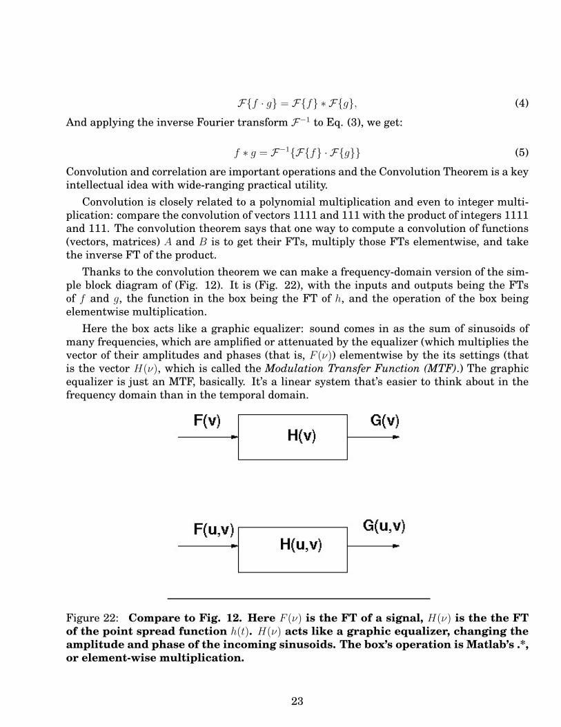
Thanks to the convolution theorem we can make a frequency-domain version of the sim-ple block diagram of (Fig. 12). It is (Fig. 22), with the inputs and outputs being the FTsof f and g, the function in the box being the FT of h, and the operation of the box beingelementwise multiplication.

Here the box acts like a graphic equalizer: sound comes in as the sum of sinusoids ofmany frequencies, which are amplified or attenuated by the equalizer (which multiplies thevector of their amplitudes and phases (that is, F (ν)) elementwise by the its settings (thatis the vector H(ν), which is called the Modulation Transfer Function (MTF).) The graphicequalizer is just an MTF, basically. It’s a linear system that’s easier to think about in thefrequency domain than in the temporal domain.

Figure 22: Compare to Fig. 12. Here F (ν) is the FT of a signal, H(ν) is the the FTof the point spread function h(t). H(ν) acts like a graphic equalizer, changing theamplitude and phase of the incoming sinusoids. The box’s operation is Matlab’s .*,or element-wise multiplication.

23

7.2 The Sampling Theorem

It makes some sort of sense, we feel, to talk about or use a sampled version of a continuousfunction. We use finite-resolution images from “x-megapixel” cameras, and film was finite-resolution too. Likewise a CD is data from a sound waveform sampled at 44KHz. MP3 isa very interesting blend of sampling and psychophysics that not only samples sound buttosses out the frequencies that it thinks you won’t miss. JPEG is similar. They are “lossyencodings”, but based on sampling.

Rising above the smog of consumer electronics trade secrets, empirical engineering hacks,and evanescent esoterica about data-encoding ’standards’, consider the idealized, mathe-matical, formalizable question: can we exactly reproduce a continuous signal from a finitenumber of samples?

We know enough now to answer that question, even if the exact algorithm isn’t clear. Ourapproach is to think in the frequency domain: every signal is a sum of sinusoids. If we couldreconstruct every sinusoid, we could reconstruct the signal. If we can reconstruct a sinusoid(its frequency, amplitude, phase) from a sequence of samples, we can surely reconstruct anylower-frequency, longer-wavelength sinusoid from the same samples (aha!!). Say there issome maximum frequency in the signal. Deconstruct the signal into sinusoids of <= thatfrequency. Find a sampling frequency f that allows recovery of the highest-frequency sinu-soid, sample the signal (thus sampling all the sinusoids) at that frequency, and reconstructthe original input from the recovered input frequencies (and phases and amplitudes).

This is a feasibility-proof, not an algorithm, but that’s all we need to answer our formalquestion: Yes, we can reconstruct a band-limited signal (one with no frequencies higher thansome maximum) exactly if we can reconstruct its highest-frequency sinusoid exactly.

Temporal Domain Argument: Imagine sampling a sine wave at its high and lowpoints, that is twice per wavelength (at twice its frequency). If you know these are thehigh and low points, you know its amplitude, phase, and frequency: you’re done. True, ifyou shift along 1/4 of a wavelength, sampling at the same rate, you’ll see a nothing but ze-roes: bad luck but no information Also notice a higher-frequency sine can sneak in betweenthe samples and not be noticed (Fig. 23).

BUT if you sample just a little faster than twice the frequency, sooner or later you’llget samples at the maximum amplitude and you can figure out all you need to know. TheNyquist frequency is twice the maximum frequency of a band-limited function and we mustsample more frequently than that to guarantee an error-free reconstruction (which can beaccomplished by interpolating between samples with a special function). In practice withfinite wave trains, 5 or 10 times the maximum frequency is a good practical sampling rateto shoot for.

Frequency Domain Argument: We use the property that the FT of the Dirac combis another Dirac comb, and that the closer the time (space) domain peaks are together, thefarther apart the frequency domain peaks are. Well, multiplying a function f(t) by the Diraccomb gives a sampled version of f(t). Using the convolution theorem (Eq. (4)), and goingto the transform domain, the transform of the sampled function is the convolution of F (ν)and the transformed Dirac comb. That is, it’s copies of F (ν), spaced apart just as far as the

24

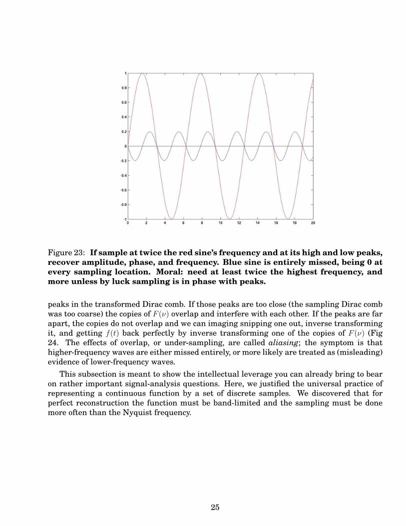
Figure 23: If sample at twice the red sine’s frequency and at its high and low peaks,recover amplitude, phase, and frequency. Blue sine is entirely missed, being 0 atevery sampling location. Moral: need at least twice the highest frequency, andmore unless by luck sampling is in phase with peaks.

peaks in the transformed Dirac comb. If those peaks are too close (the sampling Dirac combwas too coarse) the copies of F (ν) overlap and interfere with each other. If the peaks are farapart, the copies do not overlap and we can imaging snipping one out, inverse transformingit, and getting f(t) back perfectly by inverse transforming one of the copies of F (ν) (Fig24. The effects of overlap, or under-sampling, are called aliasing; the symptom is thathigher-frequency waves are either missed entirely, or more likely are treated as (misleading)evidence of lower-frequency waves.

This subsection is meant to show the intellectual leverage you can already bring to bearon rather important signal-analysis questions. Here, we justified the universal practice ofrepresenting a continuous function by a set of discrete samples. We discovered that forperfect reconstruction the function must be band-limited and the sampling must be donemore often than the Nyquist frequency.

25

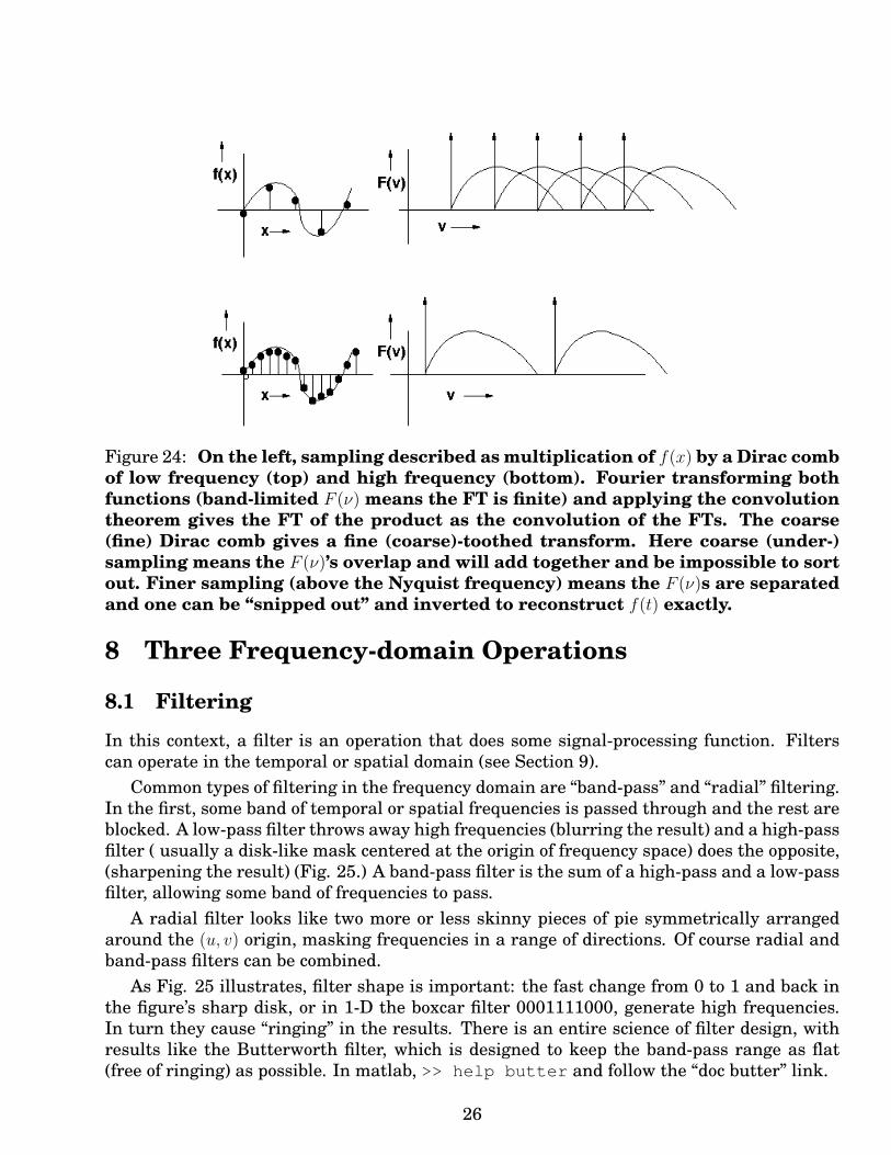
Figure 24: On the left, sampling described as multiplication of f(x) by a Dirac combof low frequency (top) and high frequency (bottom). Fourier transforming bothfunctions (band-limited F (ν) means the FT is finite) and applying the convolutiontheorem gives the FT of the product as the convolution of the FTs. The coarse(fine) Dirac comb gives a fine (coarse)-toothed transform. Here coarse (under-)sampling means the F (ν)’s overlap and will add together and be impossible to sortout. Finer sampling (above the Nyquist frequency) means the F (ν)s are separatedand one can be “snipped out” and inverted to reconstruct f(t) exactly.

8 Three Frequency-domain Operations

8.1 Filtering

In this context, a filter is an operation that does some signal-processing function. Filterscan operate in the temporal or spatial domain (see Section 9).

Common types of filtering in the frequency domain are “band-pass” and “radial” filtering.In the first, some band of temporal or spatial frequencies is passed through and the rest areblocked. A low-pass filter throws away high frequencies (blurring the result) and a high-passfilter ( usually a disk-like mask centered at the origin of frequency space) does the opposite,(sharpening the result) (Fig. 25.) A band-pass filter is the sum of a high-pass and a low-passfilter, allowing some band of frequencies to pass.

A radial filter looks like two more or less skinny pieces of pie symmetrically arrangedaround the (u, v) origin, masking frequencies in a range of directions. Of course radial andband-pass filters can be combined.

As Fig. 25 illustrates, filter shape is important: the fast change from 0 to 1 and back inthe figure’s sharp disk, or in 1-D the boxcar filter 0001111000, generate high frequencies.In turn they cause “ringing” in the results. There is an entire science of filter design, withresults like the Butterworth filter, which is designed to keep the band-pass range as flat(free of ringing) as possible. In matlab, >> help butter and follow the “doc butter” link.

26

Figure 25: Top: original image, sharp-edged high-pass filter, filtered result has ring-ing artifacts. Bottom: smooth-edged high-pass filter, result is better.

Generally, if the FT of some unwanted signal is known, it can be masked out: problemsarise because the signal you want often shares frequencies with the unwanted signal.

8.2 Matching

There is a whole science of recognizing known signals in noise (spawned when radar wasbeing developed). Some signals are better than others for radar: a reflected sine wave orpicket fence signal is ambiguous about range, an impulse signal needs a lot of power ina short time (and will be spread out when it returns). A “chirp” is a better choice, and arandom string of 1’s and -1’s isn’t bad (Fig 26).

The optimal way to detect a known signal is correlation detection, in which the input iscorrelated with the known function (or convolved with its inverse). The correlation shouldshow a peak when (or where) the known function lines up with its appearance in the input.

We met the autocorrelation of a function in Section 5.2. It is the output of correlation de-tection when the input is the known function with no noise. For instance: (remember conv

27

Figure 26: A chirp (left) has good autocorrelation properties (a sharp peak). Atright is the autocorrelation of a random string of 1’s and -1’s. In realizable func-tions, the sharp peak is flanked by “sidelobes”.

is convolution, not correlation)conv([1 2 3 4],[4 3 2 1]) = [4 11 20 30 20 11 4]. Using the time-reversal prop-erty of FTs and the convolution theorem, we get the elegant result that the power spectrumof a function is the Fourier transform of its autocorrelation.

Designing functions with good autocorrelation properties is interesting for imaging, andsignal detection. An example is finding features in images to match in automatic photo-mosaicing: they must be places you can match reliably in another image – they are smallareas with delta-function-like autocorrelations.

If the pattern to matched is small compared to the input, implementing correlation inthe time or space domain (via the 1- or 2-D shifting dot-product method) is cheaper thanFTing everything twice. Matlab has conv(), conv2() for such cases.

8.3 Image ReconstructionWithin weeks of the launch of the [big, expensive, Hubble] telescope, the re-

turned images showed that there was a serious problem with the optical system.Although the first images appeared to be sharper than ground-based images, thetelescope failed to achieve a final sharp focus, and the best image quality obtainedwas drastically lower than expected. Images of point sources spread out over a ra-dius of more than one arc-second, instead of having a point spread function (PSF)concentrated within a circle 0.1 arc-sec in diameter as had been specified in thedesign criteria.[46] The detailed performance is shown in graphs from STScI il-lustrating the mis-figured PSFs compared to post-correction and ground-basedPSFs.[47]

Analysis of the flawed images showed that the cause of the problem was thatthe primary mirror had been ground to the wrong shape. Although it was prob-ably the most precisely figured mirror ever made, with variations from the pre-

28

scribed curve of only 10 nanometers,[21] it was too flat at the edges by about2200 nanometers (2.2 microns).[48] This difference was catastrophic, introduc-ing severe spherical aberration, a flaw in which light reflecting off the edge of amirror focuses on a different point from the light reflecting off its center.[49]

–Wikipedia

How do we repair in-camera optical distortion (blurring, say) of an image? The firstground-based, signal-processing fixes to the Hubble were based on the following idea, whichstarts with the convolution theorem statement:

F{f ∗ h} = F{f} · F{h}

Let’s say the left hand side is the image from a camera with point-spread function h andscene data f . If h is an ideal Dirac delta, the output is the scene. If the camera moves duringexposure, h becomes a 2-D curve (in general), and the image is spread out along this curve.Or, if the camera is not in focus its point spread function becomes a disk. The followingargument is of course general, not just for images. Assume we know or can guess h.

In the equation above, simply divide (elementwise) by F{h}:

F{f ∗ h}F{h}

= F{f},

so

f = F−1

(F{f ∗ h}F{h}

)(6)

Here we have generated the FT of what we want (the input function) using things weknow (the point-spread function and the degraded image). Taking the inverse transformof both sides recovers the original input. It almost works. A representative example isthe box blur function, which formalizes either (in 2-D) defocus blur or (in 1-D) straight-line motion blur. Fig. 27 shows the problem: if F{h} ≈ 0, multiplying by 1

F{h} multipliesfrequencies there by huge amounts (or Inf if there is a divide by zero error). These amplifiedfrequencies often contain a noise component, so the noise can overwhelm the signal. Sosome care (thresholding before multiplying, say) is needed. The Gaussian is a very friendlyblur function since its FT is another Gaussian and so is always positive. Deconvolvingwith it simply amplifies the high frequencies, so thresholding is easy to implement and haspredictable consequences (loss of fine detail).

In crime-lab data (See Fig. 2), the PSF is the result of motion blur, and it be recoveredfrom the streak in the lower right. Here are three versions of it: the true PSF and twoapproximations.

blurmask = [ .1 .5 .9 1 1 1 1 1 1 1 1 1 1 1 1 1 1 1 1 .9 .5 .1 ] % 22 longokmask = [ 1 1 1 1 1 1 1 1 1 1 1 1 1 1 1 1 1 1 1 ] %19 longbadmask = [ 1 1 1 1 1 1 1 1 1 1 1 1 1 1 1 1 1 1 1 1 1 1 ] %22 long

The results of deconvolving and un-transforming via Eq. (6) are shown in Fig 28.

29

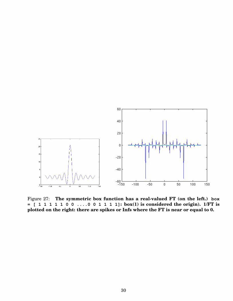
Figure 27: The symmetric box function has a real-valued FT (on the left.) box= [ 1 1 1 1 1 0 0 ....0 0 1 1 1 1]: box(1) is considered the origin). 1/FT isplotted on the right: there are spikes or Infs where the FT is near or equal to 0.

30

Figure 28: Deconvolving the motion-blurred image of Fig 2 with three possiblestreak point-spread functions (see text). Top left: badmask; top right: okmask(results serviceable but a little blurry still); Bottom: blur mask, the exact originalpoint spread function.

31

9 Time and Space-Domain Operations

While this paper is about the idea and use of transform spaces, many useful signal process-ing operations, in fact most, are performed in the time and space domains.

As an example, we might want to take the spatial derivative of the image to enhanceedges. In a digital image, that amounts to subtracting one pixel’s value from its neighbor’s.We can do that with a convolution: we just convolve with the function (or mask, in Matlabterms) [-1, 1]. So the derivative is a linear operator (which we know, given the formula ford/dx[a(f(x) + g(x))].)

Due to one of our favorite properties of eat , (its derivative is aeat), it turns out that theresult of putting the derivative operator into the FT is a cone-shaped function in frequencyspace rising from 0 at the origin and proportional to the frequency. The in frequency space,the derivative is a graphic equalizer that amplifies sinusoids by a factor proportional to theirfrequency. Makes sense: the derivative of slowly-varying waves is small, and of fast-varyingones is big.

Practically speaking, it is quicker and easier (takes fewer computer operations) to dothe this little convolution in the space domain than it does to transform, multiply, and un-transform image-sized matrices. Further, this filter like many can be implemented as a ’realtime’ operation rather than a ’batch’ operation: d/dt can be done ’on the fly’ by streamingthe signal through a little circuit that subtracts neighboring data values and outputs theresults. Likewise more complex filters like guitar effects are real-time circuits with a littlememory.

As an experimentalist, you will be fitting mathematical models to experimental data,smoothing or interpolating data, creating statistics and visualizations. As we have seen,frequency space certainly has its uses, but unless frequencies are the issue you may neverfind yourself in transform space.

In sound processing, basic temporal-domain operations include overdubbing, sampling,splicing, amplitude modulation, “loop delays”, and guitar effects like phasers and flangers.

Is spatial processing useful for images? Well, imagine inserting the Photoshop manualright here. So yes. Matlab has an image processing toolbox, with some very useful proventechniques, like Mathematical morphology, which is like convolution but the operations arenon-linear set operations like AND and OR functions over the data (binary data is the eas-iest to think about). Morphology is excellent for cleaning up noisy images in many usefulways, and also can be used for matching.

Enough. There is much more to be learned and used, but I hope you have an inkling ofwhy transform spaces are useful in many contexts, especially signal processing.

10 Sources and References

Mathematical Morphology: Theory and Hardware (Oxford Series in Optical and ImagingSciences); R. M. Haralick; Oxford U. Press 2010.

32

Digital Image Processing using Matlab; R.C. Gonzalez, R.E. Woods, S. L. Eddins; Pearson2004.

Computer Vision and Image Processing: a practical approach using CVIPtools; S.E. Um-baugh, Prentice-Hall 1998

Digital Image Processing, 2nd Ed.; R.C. Gonzalez, R.E. Woods; Prentice-Hall 2002.Digital Image Processing; K.R. Castleman; Prentice-Hall 1996.Digital Image Processing,3rd Ed.; W.K. Pratt, Wiley 2001.Traitement numerique des images; M. Kunt, G. Granlund, M. Kocher; Presses polytech-

niques et universitaires romandes 1993.Brown, C.M., “Multiplex imaging with multiple pinhole cameras,” J. Appl. Physics 45, 4

April 1974.Brown, C.M., “An iterative improvement algorithm for coherent codes,” Optics Commu-

nications 33, 3, 241-244, June 1980.

http://fourier.eng.hmc.edu/e101/lectures/Fourier_Analysis/Fourier_Analysis.htmlgood tutorialhttp://sharp.bu.edu/˜slehar/fourier/fourier.htmlnice examples, good tutorialhttp://mrl.nyu.edu/˜dzorin/intro-graphics/handouts/filtering/node3.htmlhttp://en.wikipedia.org/wiki/Phasor_%28sine_waves%29http://en.wikipedia.org/wiki/Dirac_delta_function

http://terpconnect.umd.edu/˜toh/spectrum/TOC.htmlillustrated, browseable, 45-page essay on Signal processing inchemical analysis, with code and examples.

http://local.wasp.uwa.edu.au/˜pbourke/miscellaneous/imagefilter/

Wikipedia: Coma, Distortion, Convolution (animation), Phasor (animation), Dirac DeltaFunction, dot product, Euler’s formula, etc.

A Complex Numbers

Complex numbers are just mathematical objects, like integers, reals, and matrices, thathave their own algebraic rules. A complex number is of the form a + bi, where i is

√−1.

Especially in engineering, i is often called j. Complex numbers were controversial whenintroduced by Cardano back in the 1500’s, and they still resist ’understanding’ about whatthey ’really’ are. Maybe there’s a ’Metaphysics of Mathematics’ course that worries aboutthat, but it’s best to think of them as Useful Gadgets That Do The Right Thing.

For instance, there isn’t anything wrong with the equation x2 = 1: the answer’s x = ±1.By analogy, what’s wrong with the equation x2 = −1? Nothing, except you won’t find an

33

integer, fraction, real number, matrix, etc. that solves it. But it is solved by x = ±i if youdefine i such that i2 = −1. So think of it as a formal shorthand solution for a (mind-bendingbut) simple mathematical problem. You may recall that the solution to a simple quadraticequation ax2 + bx+ c = 0 is complex if

√b2 − 4ac < 0: in fact it is ((−b/2a)± (i/2a)

√b2 − 4ac).

Or, if you’re still queasy with√−1, you can just define a complex number as an (a, b) pair

of real numbers, use the rules below to define operations on the pair.A complex number a + bi can be considered to live in a plane with a real-part axis (giv-

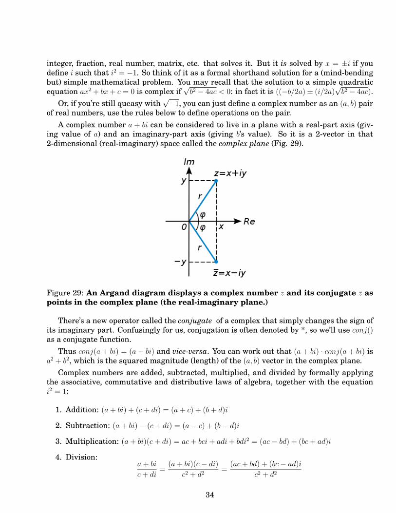
ing value of a) and an imaginary-part axis (giving b’s value). So it is a 2-vector in that2-dimensional (real-imaginary) space called the complex plane (Fig. 29).

Figure 29: An Argand diagram displays a complex number z and its conjugate z̄ aspoints in the complex plane (the real-imaginary plane.)

There’s a new operator called the conjugate of a complex that simply changes the sign ofits imaginary part. Confusingly for us, conjugation is often denoted by *, so we’ll use conj()as a conjugate function.

Thus conj(a + bi) = (a− bi) and vice-versa. You can work out that (a + bi) · conj(a + bi) isa2 + b2, which is the squared magnitude (length) of the (a, b) vector in the complex plane.

Complex numbers are added, subtracted, multiplied, and divided by formally applyingthe associative, commutative and distributive laws of algebra, together with the equationi2 = 1:

1. Addition: (a+ bi) + (c+ di) = (a+ c) + (b+ d)i

2. Subtraction: (a+ bi)− (c+ di) = (a− c) + (b− d)i

3. Multiplication: (a+ bi)(c+ di) = ac+ bci+ adi+ bdi2 = (ac− bd) + (bc+ ad)i

4. Division:a+ bi

c+ di=

(a+ bi)(c− di)c2 + d2

=(ac+ bd) + (bc− ad)i

c2 + d2

34

where c and d are not both zero. Derive this by multiplying both the numerator andthe denominator by the conjugate of the denominator (c+ di), which is (cdi).

If you’re reading this, you know that complex numbers have come up in the signalprocessing context. They’re ubiquitous so you’ve got to get used to them. As always,consult your favorite text or Wikipedia (’Complex Numbers’) for more.

B Power Spectrum Examples

These are meant to highlight frequency-domain features and how they are related to theirimage (spatial domain) counterparts. The power spectrum has a wide range of values andmust be manipulated in order to be shown. Here I zeroed out the central peak (always huge,representing the sum of all image values), added 1 to all the values, took their logarithm,then scaled the values to [0,1].

The vertical line in the Limbaugh power spectrum and the horizontal one in the beachsand are doubtless artifacts having to do with image cropping.

35

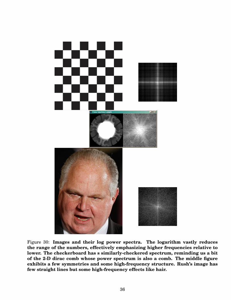
Figure 30: Images and their log power spectra. The logarithm vastly reducesthe range of the numbers, effectively emphasizing higher frequencies relative tolower. The checkerboard has s similarly-checkered spectrum, reminding us a bitof the 2-D dirac comb whose power spectrum is also a comb. The middle figureexhibits a few symmetries and some high-frequency structure. Rush’s image hasfew straight lines but some high-frequency effects like hair.

36

Figure 31: Images and their log power spectra. We expect the sand image to haverelatively much high-frequency power in no specific direction, and that the build-ing and basket exhibit some straight line power spikes and 4-fold periodicity.

37