information and entropy in quantum theory · 2002-07-04 · abstract recent developments in quantum...
TRANSCRIPT

Information and Entropy in Quantum Theory
O J E Maroney
Ph.D. Thesis
Birkbeck College
University of London
Malet Street
London
WC1E 7HX

Abstract
Recent developments in quantum computing have revived interest in the notion of information
as a foundational principle in physics. It has been suggested that information provides a means of
interpreting quantum theory and a means of understanding the role of entropy in thermodynam-
ics. The thesis presents a critical examination of these ideas, and contrasts the use of Shannon
information with the concept of ’active information’ introduced by Bohm and Hiley.
We look at certain thought experiments based upon the ’delayed choice’ and ’quantum eraser’
interference experiments, which present a complementarity between information gathered from a
quantum measurement and interference effects. It has been argued that these experiments show
the Bohm interpretation of quantum theory is untenable. We demonstrate that these experiments
depend critically upon the assumption that a quantum optics device can operate as a measuring
device, and show that, in the context of these experiments, it cannot be consistently understood
in this way. By contrast, we then show how the notion of ’active information’ in the Bohm
interpretation provides a coherent explanation of the phenomena shown in these experiments.
We then examine the relationship between information and entropy. The thought experiment
connecting these two quantities is the Szilard Engine version of Maxwell’s Demon, and it has been
suggested that quantum measurement plays a key role in this. We provide the first complete
description of the operation of the Szilard Engine as a quantum system. This enables us to
demonstrate that the role of quantum measurement suggested is incorrect, and further, that the
use of information theory to resolve Szilard’s paradox is both unnecessary and insufficient. Finally
we show that, if the concept of ’active information’ is extended to cover thermal density matrices,
then many of the conceptual problems raised by this paradox appear to be resolved.
1

Contents
1 Introduction 10
2 Information and Measurement 13
2.1 Shannon Information . . . . . . . . . . . . . . . . . . . . . . . . . . . . . . . . . . . 13
2.1.1 Communication . . . . . . . . . . . . . . . . . . . . . . . . . . . . . . . . . . 15
2.1.2 Measurements . . . . . . . . . . . . . . . . . . . . . . . . . . . . . . . . . . 16
2.2 Quantum Information . . . . . . . . . . . . . . . . . . . . . . . . . . . . . . . . . . 17
2.2.1 Quantum Communication Capacity . . . . . . . . . . . . . . . . . . . . . . 17
2.2.2 Information Gain . . . . . . . . . . . . . . . . . . . . . . . . . . . . . . . . . 18
2.2.3 Quantum Information Quantities . . . . . . . . . . . . . . . . . . . . . . . . 20
2.2.4 Measurement . . . . . . . . . . . . . . . . . . . . . . . . . . . . . . . . . . . 22
2.3 Quantum Measurement . . . . . . . . . . . . . . . . . . . . . . . . . . . . . . . . . 24
2.4 Summary . . . . . . . . . . . . . . . . . . . . . . . . . . . . . . . . . . . . . . . . . 29
3 Active Information and Interference 30
3.1 The Quantum Potential as an Information Potential . . . . . . . . . . . . . . . . . 31
3.1.1 Non-locality . . . . . . . . . . . . . . . . . . . . . . . . . . . . . . . . . . . . 31
3.1.2 Form dependence . . . . . . . . . . . . . . . . . . . . . . . . . . . . . . . . . 32
3.1.3 Active, Passive and Inactive Information . . . . . . . . . . . . . . . . . . . . 33
3.2 Information and interference . . . . . . . . . . . . . . . . . . . . . . . . . . . . . . . 34
3.2.1 The basic interferometer . . . . . . . . . . . . . . . . . . . . . . . . . . . . . 35
3.2.2 Which way information . . . . . . . . . . . . . . . . . . . . . . . . . . . . . 37
3.2.3 Welcher-weg devices . . . . . . . . . . . . . . . . . . . . . . . . . . . . . . . 39
3.2.4 Surrealistic trajectories . . . . . . . . . . . . . . . . . . . . . . . . . . . . . 43
3.2.5 Conclusion . . . . . . . . . . . . . . . . . . . . . . . . . . . . . . . . . . . . 48
3.3 Information and which path measurements . . . . . . . . . . . . . . . . . . . . . . 48
3.3.1 Which path information . . . . . . . . . . . . . . . . . . . . . . . . . . . . . 49
3.3.2 Welcher-weg information . . . . . . . . . . . . . . . . . . . . . . . . . . . . . 52
3.3.3 Locality and teleportation . . . . . . . . . . . . . . . . . . . . . . . . . . . . 55
3.3.4 Conclusion . . . . . . . . . . . . . . . . . . . . . . . . . . . . . . . . . . . . 59
2

3.4 Conclusion . . . . . . . . . . . . . . . . . . . . . . . . . . . . . . . . . . . . . . . . 62
4 Entropy and Szilard’s Engine 64
4.1 Statistical Entropy . . . . . . . . . . . . . . . . . . . . . . . . . . . . . . . . . . . . 65
4.2 Maxwell’s Demon . . . . . . . . . . . . . . . . . . . . . . . . . . . . . . . . . . . . . 67
4.2.1 Information Acquisition . . . . . . . . . . . . . . . . . . . . . . . . . . . . . 68
4.2.2 Information Erasure . . . . . . . . . . . . . . . . . . . . . . . . . . . . . . . 69
4.2.3 ”Demonless” Szilard Engine . . . . . . . . . . . . . . . . . . . . . . . . . . . 72
4.3 Conclusion . . . . . . . . . . . . . . . . . . . . . . . . . . . . . . . . . . . . . . . . 76
5 The Quantum Mechanics of Szilard’s Engine 79
5.1 Particle in a box . . . . . . . . . . . . . . . . . . . . . . . . . . . . . . . . . . . . . 81
5.2 Box with Central Barrier . . . . . . . . . . . . . . . . . . . . . . . . . . . . . . . . 82
5.2.1 Asymptotic solutions for the HBA, V À E . . . . . . . . . . . . . . . . . . 86
5.3 Moveable Partition . . . . . . . . . . . . . . . . . . . . . . . . . . . . . . . . . . . . 87
5.3.1 Free Piston . . . . . . . . . . . . . . . . . . . . . . . . . . . . . . . . . . . . 88
5.3.2 Piston and Gas on one side . . . . . . . . . . . . . . . . . . . . . . . . . . . 90
5.3.3 Piston with Gas on both sides . . . . . . . . . . . . . . . . . . . . . . . . . 93
5.4 Lifting a weight against gravity . . . . . . . . . . . . . . . . . . . . . . . . . . . . . 98
5.5 Resetting the Engine . . . . . . . . . . . . . . . . . . . . . . . . . . . . . . . . . . . 102
5.5.1 Inserting Shelves . . . . . . . . . . . . . . . . . . . . . . . . . . . . . . . . . 103
5.5.2 Removing the Piston . . . . . . . . . . . . . . . . . . . . . . . . . . . . . . . 106
5.5.3 Resetting the Piston . . . . . . . . . . . . . . . . . . . . . . . . . . . . . . . 106
5.6 Conclusions . . . . . . . . . . . . . . . . . . . . . . . . . . . . . . . . . . . . . . . . 111
5.6.1 Raising Cycle . . . . . . . . . . . . . . . . . . . . . . . . . . . . . . . . . . . 112
5.6.2 Lowering Cycle . . . . . . . . . . . . . . . . . . . . . . . . . . . . . . . . . . 113
5.6.3 Summary . . . . . . . . . . . . . . . . . . . . . . . . . . . . . . . . . . . . . 114
6 The Statistical Mechanics of Szilard’s Engine 116
6.1 Statistical Mechanics . . . . . . . . . . . . . . . . . . . . . . . . . . . . . . . . . . . 117
6.2 Thermal state of gas . . . . . . . . . . . . . . . . . . . . . . . . . . . . . . . . . . . 120
6.2.1 No partition . . . . . . . . . . . . . . . . . . . . . . . . . . . . . . . . . . . . 121
6.2.2 Partition raised . . . . . . . . . . . . . . . . . . . . . . . . . . . . . . . . . . 121
6.2.3 Confined Gas . . . . . . . . . . . . . . . . . . . . . . . . . . . . . . . . . . . 122
6.2.4 Moving partition . . . . . . . . . . . . . . . . . . . . . . . . . . . . . . . . . 123
6.3 Thermal State of Weights . . . . . . . . . . . . . . . . . . . . . . . . . . . . . . . . 128
6.3.1 Raising and Lowering Weight . . . . . . . . . . . . . . . . . . . . . . . . . . 128
6.3.2 Inserting Shelf . . . . . . . . . . . . . . . . . . . . . . . . . . . . . . . . . . 131
6.3.3 Mean Energy of Projected Weights . . . . . . . . . . . . . . . . . . . . . . . 132
3

6.4 Gearing Ratio of Piston to Pulley . . . . . . . . . . . . . . . . . . . . . . . . . . . . 134
6.4.1 Location of Unraised Weight . . . . . . . . . . . . . . . . . . . . . . . . . . 135
6.5 The Raising Cycle . . . . . . . . . . . . . . . . . . . . . . . . . . . . . . . . . . . . 135
6.6 The Lowering Cycle . . . . . . . . . . . . . . . . . . . . . . . . . . . . . . . . . . . 141
6.7 Energy Flow in Popper-Szilard Engine . . . . . . . . . . . . . . . . . . . . . . . . . 144
6.8 Conclusion . . . . . . . . . . . . . . . . . . . . . . . . . . . . . . . . . . . . . . . . 150
7 The Thermodynamics of Szilard’s Engine 152
7.1 Free Energy and Entropy . . . . . . . . . . . . . . . . . . . . . . . . . . . . . . . . 153
7.1.1 One Atom Gas . . . . . . . . . . . . . . . . . . . . . . . . . . . . . . . . . . 154
7.1.2 Weight above height h . . . . . . . . . . . . . . . . . . . . . . . . . . . . . . 156
7.1.3 Correlations and Mixing . . . . . . . . . . . . . . . . . . . . . . . . . . . . . 157
7.2 Raising cycle . . . . . . . . . . . . . . . . . . . . . . . . . . . . . . . . . . . . . . . 160
7.3 Lowering Cycle . . . . . . . . . . . . . . . . . . . . . . . . . . . . . . . . . . . . . . 165
7.4 Conclusion . . . . . . . . . . . . . . . . . . . . . . . . . . . . . . . . . . . . . . . . 168
8 Resolution of the Szilard Paradox 169
8.1 The Role of the Demon . . . . . . . . . . . . . . . . . . . . . . . . . . . . . . . . . 170
8.1.1 The Role of the Piston . . . . . . . . . . . . . . . . . . . . . . . . . . . . . . 170
8.1.2 Maxwell’s Demons . . . . . . . . . . . . . . . . . . . . . . . . . . . . . . . . 172
8.1.3 The Significance of Mixing . . . . . . . . . . . . . . . . . . . . . . . . . . . 173
8.1.4 Generalised Demon . . . . . . . . . . . . . . . . . . . . . . . . . . . . . . . . 179
8.1.5 Conclusion . . . . . . . . . . . . . . . . . . . . . . . . . . . . . . . . . . . . 183
8.2 Restoring the Auxiliary . . . . . . . . . . . . . . . . . . . . . . . . . . . . . . . . . 184
8.2.1 Fluctuation Probability Relationship . . . . . . . . . . . . . . . . . . . . . . 184
8.2.2 Imperfect Resetting . . . . . . . . . . . . . . . . . . . . . . . . . . . . . . . 187
8.2.3 The Carnot Cycle and the Entropy Engine . . . . . . . . . . . . . . . . . . 199
8.2.4 Conclusion . . . . . . . . . . . . . . . . . . . . . . . . . . . . . . . . . . . . 201
8.3 Alternative resolutions . . . . . . . . . . . . . . . . . . . . . . . . . . . . . . . . . . 202
8.3.1 Information Acquisition . . . . . . . . . . . . . . . . . . . . . . . . . . . . . 202
8.3.2 Information Erasure . . . . . . . . . . . . . . . . . . . . . . . . . . . . . . . 204
8.3.3 ’Free will’ and Computation . . . . . . . . . . . . . . . . . . . . . . . . . . . 207
8.3.4 Quantum superposition . . . . . . . . . . . . . . . . . . . . . . . . . . . . . 210
8.4 Comments and Conclusions . . . . . . . . . . . . . . . . . . . . . . . . . . . . . . . 215
8.4.1 Criticisms of the Resolution . . . . . . . . . . . . . . . . . . . . . . . . . . . 215
8.4.2 Summary . . . . . . . . . . . . . . . . . . . . . . . . . . . . . . . . . . . . . 217
9 Information and Computation 219
9.1 Reversible and tidy computations . . . . . . . . . . . . . . . . . . . . . . . . . . . . 219
4

9.1.1 Landauer Erasure . . . . . . . . . . . . . . . . . . . . . . . . . . . . . . . . 220
9.1.2 Tidy classical computations . . . . . . . . . . . . . . . . . . . . . . . . . . . 223
9.1.3 Tidy quantum computations . . . . . . . . . . . . . . . . . . . . . . . . . . 224
9.1.4 Conclusion . . . . . . . . . . . . . . . . . . . . . . . . . . . . . . . . . . . . 227
9.2 Thermodynamic and logical reversibility . . . . . . . . . . . . . . . . . . . . . . . . 227
9.2.1 Thermodynamically irreversible computation . . . . . . . . . . . . . . . . . 228
9.2.2 Logically irreversible operations . . . . . . . . . . . . . . . . . . . . . . . . . 228
9.3 Conclusion . . . . . . . . . . . . . . . . . . . . . . . . . . . . . . . . . . . . . . . . 230
10 Active Information and Entropy 232
10.1 The Statistical Ensemble . . . . . . . . . . . . . . . . . . . . . . . . . . . . . . . . . 232
10.2 The Density Matrix . . . . . . . . . . . . . . . . . . . . . . . . . . . . . . . . . . . 235
10.2.1 Szilard Box . . . . . . . . . . . . . . . . . . . . . . . . . . . . . . . . . . . . 236
10.2.2 Correlations and Measurement . . . . . . . . . . . . . . . . . . . . . . . . . 237
10.3 Active Information . . . . . . . . . . . . . . . . . . . . . . . . . . . . . . . . . . . . 238
10.3.1 The Algebraic Approach . . . . . . . . . . . . . . . . . . . . . . . . . . . . . 239
10.3.2 Correlations and Measurement . . . . . . . . . . . . . . . . . . . . . . . . . 242
10.4 Conclusion . . . . . . . . . . . . . . . . . . . . . . . . . . . . . . . . . . . . . . . . 248
A Quantum State Teleportation 250
A.1 Introduction . . . . . . . . . . . . . . . . . . . . . . . . . . . . . . . . . . . . . . . . 250
A.2 Quantum Teleportation . . . . . . . . . . . . . . . . . . . . . . . . . . . . . . . . . 251
A.3 Quantum State Teleportation and Active Information . . . . . . . . . . . . . . . . 252
A.4 Conclusion . . . . . . . . . . . . . . . . . . . . . . . . . . . . . . . . . . . . . . . . 255
B Consistent histories and the Bohm approach 257
B.1 Introduction . . . . . . . . . . . . . . . . . . . . . . . . . . . . . . . . . . . . . . . . 257
B.2 Histories and trajectories . . . . . . . . . . . . . . . . . . . . . . . . . . . . . . . . 258
B.3 The interference experiment . . . . . . . . . . . . . . . . . . . . . . . . . . . . . . . 260
B.4 Conclusion . . . . . . . . . . . . . . . . . . . . . . . . . . . . . . . . . . . . . . . . 264
C Unitary Evolution Operators 265
D Potential Barrier Solutions 268
D.1 Odd symmetry . . . . . . . . . . . . . . . . . . . . . . . . . . . . . . . . . . . . . . 270
D.1.1 E > V . . . . . . . . . . . . . . . . . . . . . . . . . . . . . . . . . . . . . . . 270
D.1.2 E = V . . . . . . . . . . . . . . . . . . . . . . . . . . . . . . . . . . . . . . . 271
D.1.3 E < V . . . . . . . . . . . . . . . . . . . . . . . . . . . . . . . . . . . . . . . 272
D.1.4 Summary . . . . . . . . . . . . . . . . . . . . . . . . . . . . . . . . . . . . . 273
D.2 Even symmetry . . . . . . . . . . . . . . . . . . . . . . . . . . . . . . . . . . . . . . 273
5

D.2.1 E > V . . . . . . . . . . . . . . . . . . . . . . . . . . . . . . . . . . . . . . 273
D.2.2 E = V . . . . . . . . . . . . . . . . . . . . . . . . . . . . . . . . . . . . . . . 274
D.2.3 E < V . . . . . . . . . . . . . . . . . . . . . . . . . . . . . . . . . . . . . . . 275
D.2.4 Summary . . . . . . . . . . . . . . . . . . . . . . . . . . . . . . . . . . . . . 276
D.3 Numerical Solutions to Energy Eigenvalues . . . . . . . . . . . . . . . . . . . . . . 276
E Energy of Perturbed Airy Functions 279
F Energy Fluctuations 282
G Free Energy and Temperature 285
H Free Energy and Non-Equilibrium Systems 290
6

List of Figures
3.1 Basic Interferometer . . . . . . . . . . . . . . . . . . . . . . . . . . . . . . . . . . . 35
3.2 Which-path delayed choice . . . . . . . . . . . . . . . . . . . . . . . . . . . . . . . . 39
3.3 Welcher-weg cavities . . . . . . . . . . . . . . . . . . . . . . . . . . . . . . . . . . . 42
3.4 Surrealistic Trajectories . . . . . . . . . . . . . . . . . . . . . . . . . . . . . . . . . 44
4.1 The Szilard Engine . . . . . . . . . . . . . . . . . . . . . . . . . . . . . . . . . . . . 68
4.2 Landauer Bit and Logical Measurement . . . . . . . . . . . . . . . . . . . . . . . . 70
4.3 Bit Erasure . . . . . . . . . . . . . . . . . . . . . . . . . . . . . . . . . . . . . . . . 72
4.4 The Popper version of Szilard’s Engine . . . . . . . . . . . . . . . . . . . . . . . . . 73
4.5 The Cycle of the Popper-Szilard Engine . . . . . . . . . . . . . . . . . . . . . . . . 77
5.1 Superpositions of odd and even symmetry states . . . . . . . . . . . . . . . . . . . 85
5.2 Asymptotic Values of Energy Levels . . . . . . . . . . . . . . . . . . . . . . . . . . 87
5.3 Motion of Piston . . . . . . . . . . . . . . . . . . . . . . . . . . . . . . . . . . . . . 89
5.4 Airy Functions for a Mass in Gravitational Field . . . . . . . . . . . . . . . . . . . 99
5.5 Splitting Airy Function at Height h . . . . . . . . . . . . . . . . . . . . . . . . . . . 104
5.6 Correlation of Weights and Piston Position . . . . . . . . . . . . . . . . . . . . . . 109
5.7 The Lowering Cycle of the Popper-Szilard Engine . . . . . . . . . . . . . . . . . . 115
6.1 Mean Flow of Energy in Popper-Szilard Engine . . . . . . . . . . . . . . . . . . . . 147
7.1 Change in Entropy on Raising Cycle . . . . . . . . . . . . . . . . . . . . . . . . . . 164
7.2 Change in Entropy on Lowering Cycle . . . . . . . . . . . . . . . . . . . . . . . . . 168
9.1 Distributed quantum computing . . . . . . . . . . . . . . . . . . . . . . . . . . . . 225
B.1 Simple interferometer . . . . . . . . . . . . . . . . . . . . . . . . . . . . . . . . . . 258
B.2 The CH ‘trajectories’. . . . . . . . . . . . . . . . . . . . . . . . . . . . . . . . . . . 259
B.3 The Bohm trajectories. . . . . . . . . . . . . . . . . . . . . . . . . . . . . . . . . . . 260
D.1 First six energy eigenvalues with potential barrier . . . . . . . . . . . . . . . . . . . 277
D.2 Perturbation of Even Symmetry Eigenstates . . . . . . . . . . . . . . . . . . . . . . 278
D.3 Degeneracy of Even and Odd Symmetry Eigenstates . . . . . . . . . . . . . . . . . 278
7

G.1 The Entropy Engine . . . . . . . . . . . . . . . . . . . . . . . . . . . . . . . . . . . 288
8

List of Tables
4.1 The Controlled Not Gate . . . . . . . . . . . . . . . . . . . . . . . . . . . . . . . . 71
6.1 Work extracted from gas . . . . . . . . . . . . . . . . . . . . . . . . . . . . . . . . . 126
7.1 Thermodynamic Properties of the Raising Cycle . . . . . . . . . . . . . . . . . . . 164
7.2 Thermodynamic Properties of Lowering Cycle . . . . . . . . . . . . . . . . . . . . 167
9

Chapter 1
Introduction
In recent years there has been a significant interest in the idea of information as fundamental
principle in physics[Whe83, Whe90, Zur90b, Per93, FS95, Fri98, Deu97, Zei99, Sto90, Sto92, Sto97,
amongst others]. While much of this interest has been driven by the developments in quantum
computation[Gru99, CN01] the issues that are addressed are old ones. In particular, it has been
suggested that:
1. Information theory must be introduced into physical theories at the same fundamental level
as concepts such as energy;
2. Information theory provides a resolution to the measurement problem in quantum mechanics;
3. Thermodynamic entropy is equivalent to information, and that information theory is essential
to exorcising Maxwell’s Demon.
The concept of information used in these suggestions is essentially that introduced by Shannon[Sha48]
and it’s generalisation to quantum theory by Schumacher[Sch95]. This concept was originally con-
cerned with the use of different signals to communicate messages, and the capacity of physical
systems to carry these signals, and is a largely static property of statistical ensembles.
A completely different concept of information was introduced by Bohm and Hiley[BH93] in the
context of Bohm’s interpretation of quantum theory[Boh52a, Boh52b]. This concept was much
more dynamic, as it concerned the manner in which an individual system evolves.
In this thesis we will be examining some of these relationships between information, thermo-
dynamic entropy, and quantum theory. We will use information to refer to Shannon-Schumacher
information, and active information to refer to Bohm and Hiley’s concept. We will not be examining
the ideas of Fisher information[Fis25, Fri88, Fri89, FS95, Fri98, Reg98], although it is interesting to
note that the terms that result from applying this to quantum theory bear a remarkable equivalence
to the quantum potential term in the Bohm approach. Similarly, we will not be considering the
recently introduced idea of total information due to Bruckner and Zeilinger[BZ99, BZ00a, BZ00b].
We will also leave aside the concept of algorithmic information[Ben82, Zur89a, Zur89b, Zur90a,
10


Finally in Chapter 10 we will re-examine the concept of active information to see if it has any rel-
evance to thermodynamics. We will find that recent developments of the Bohm interpretation[BH00]
suggest that the problems surrounding the Szilard Engine may be viewed in a new light using the
concept of active information. The fundamental conflict in interpreting thermodynamics is be-
tween the statistical ensemble description, and the state of the individual system. We will show
that, by extending Bohm’s interpretation to include the quantum mechanical density matrix we
can remove this conflict in a manner that is not available to classical statistical mechanics and
does not appear to be available to other interpretations of quantum theory.
With regard to the three issues raised above, therefore, we will have found that:
1. The introduction of information as a fundamental principle in physics certainly provides a
useful heuristic device. However, to be fruitful a much wider concept of information than
Shannon’s seems to be required, such as that provided by Bohm and Hiley;
2. The use of Shannon-Schumacher information in a physical theory must presume the existence
of a well defined measurement procedure. Until a measurement can be certain to have taken
place, no information can be gained. Information theoretic attempts to resolve the quantum
measurement problem are therefore essentially circular unless they use a notion of information
that goes beyond Shannon and Schumacher;
3. Although Shannon-Schumacher information and Gibbs-Von Neumann entropy are formally
similar they apply to distinctly different concepts. As an information processing system must
be implemented upon a physical system, it is bound by physical laws and in an appropriate
limit they become related by Landauer’s Principle. Even in this limit, though, the different
nature of the concepts persists.
12

Chapter 2
Information and Measurement
In this Chapter we will briefly review the concept of Shannon information[Sha48, SW49] and it’s
application to quantum theory.
Section 1 reviews the classical notion of information introduced by Shannon and it’s key fea-
tures. Section 2 looks at the application of Shannon information to the outcomes of quantum
measurements[Kul59, Per93, Gru99, CN01]. We will be assuming that a quantum measurement
is a well defined process. The Shannon measure may be generalised to Schumacher information,
but the interpretation of some of the quantities that are constructed from such a generalisation
remains unclear. Finally in Section 3 we will consider an attempt by [AC97] to use the quantum
information measures to resolve the measurement problem, and show that this fails.
2.1 Shannon Information
Shannon information was original defined to solve the problem of the most efficient coding of a
set of signals[SW49, Sha48]. We suppose that there is a source of signals (or sender) who will
transmit a given message a with probability Pa. The message will be represented by a bit string
(an ordered series of 1’s and 0’s). The receiver will have a decoder that will convert the bit string
back into it’s corresponding message. Shannon’s theorem shows that the mean length of the bit
strings can be compressed to a size
ISh = −∑
a
pa log2 pa (2.1)
without introducing the possibility of errors in the decoded message1. This quantity ISh is
called the Shannon information of the source. As it refers to the length in bits, per message, into
which the messages can be compressed, then a communication channel that transmits ISh bits per
message has a signal capacity of ISh.1This assumes there is no noise during transmission.
13

This concept of information has no relationship to the meaning or significance that the sender
or the receiver attributes to the message itself. The information content of a particular signal,
− log2 pa, is simply an expression of how likely, or unlikely the message is of being sent. The less
likely the occurrence of a message, the greater information it conveys. In the limit where a message
is certain to occur (Pa = 1), then no information is conveyed by it, as the receiver would have
known in advance that it was going to be received. An extremely rare message conveys a great deal
of information as it tells the receiver that a very unlikely state of affairs exists. In many respects,
the Shannon information of the message can be regarded as measuring the ’surprise’ the receiver
feels on reading the message!
The most important properties of the Shannon information, however, are expressed in terms
of conditional I(α|β) and mutual I(α : β) information, where two variables α and β are being
considered. The probability of the particular values of α = a and β = b simultaneously occurring
is given by P (a, b), and the joint information is therefore
I(α, β) = −∑
a,b
P (a, b) log2 P (a, b)
From the joint probability distribution P (a, b) we construct the separate probability distributions
P (a) =∑
b
P (a, b)
P (b) =∑
a
P (a, b)
the conditional probabilities
P (a|b) =P (a, b)P (b)
P (b|a) =P (a, b)P (a)
and the correlation
P (a : b) =P (a, b)
P (a)P (b)
This leads to the information terms2
I(α) = −∑
a,b
P (a, b) log2 P (a)
I(β) = −∑
a,b
P (a, b) log2 P (b)
I(α|β) = −∑
a,b
P (a, b) log2 P (a|b)
I(β|α) = −∑
a,b
P (a, b) log2 P (b|a)
I(α : β) = −∑
a,b
P (a, b) log2 P (a : b)
2These terms may differ by the minus sign from the definitions given elsewhere. The Shannon information as
given represents the ignorance about the exact state of the system.
14

which are related by
I(α|β) = I(α, β)− I(β)
I(β|α) = I(α, β)− I(α)
I(α : β) = I(α, β)− I(α)− I(β)
and obey the inequalities
I(α, β) ≥ I(α) ≥ 0
I(α, β) ≥ I(α|β) ≥ 0
min [I(α), I(β)] ≥ −I(α : β) ≥ 0
We can interpret these relationships, and the α and β variables, as representing communication
between two people, or as the knowledge a single person has of the state of a physical system.
2.1.1 Communication
If β represents the signal states that the sender transmits, and α represents the outcomes of the
receivers attempt to decode the message, then P (a|b) represents the reliability of the transmission
and decoding3.
The receiver initially estimates the probability of a particular signal being transmitted as P (b),
and so has information I(β). After decoding, the receiver has found the state a. Presumably
knowing the reliability of the communication channel, she may now use Bayes’s rule to re-estimate
the probability of the transmitted signals
P (b|a) =P (a|b)P (b)
P (a)
On receiving the result a, therefore, the receiver has information
I(β|a) =∑
b
P (b|a) log2 P (b|a)
about the signal sent. Her information gain, is
∆Ia(β) = I(β|a)− I(β) (2.2)
Over an ensemble of such signals, the result a will occur with probability P (a). The mean infor-
mation possessed by the receiver is then
〈I(β|a)〉 =∑
a
P (a)I(β|a) = I(β|α)
So the conditional information I(β|α) represents the average information the receiver possesses
about the signal state, given her knowledge of the received state, while the term I(β|a) represents
3There are many ways in which the decoding may be unreliable. The communication channel may be noisy, the
decoding mechanism may not be optimally designed, and the signal states may be overlapping in phase space
15

the information the receiver possesses given a specific outcome a. The mean information gain
〈∆I(β|a)〉 =∑
a
P (a)∆Ia(β) = I(α : β)
The mutual information is the gain in information the receiver has about the signal sent. It can be
shown that, given that the sender is also aware of the reliability of the transmission and decoding
process, that the conditional information I(α|β) represents the knowledge the sender has about
the signal the receiver actually receives. The mutual information can then be regarded as the
symmetric function expressing the information both receiver and sender possess in common, or
equivalently, the correlation between the state of the sender and the state of the receiver.
If the transmission and decoding processes are completely reliable, then the particular receiver
states of α will be in a one-to-one correspondence with the signal states of β, with probabilities
P (a|b) = 1. This leads to
I(α) = I(β)
I(β|α) = I(α|β) = 0
I(α : β) = −I(α)
It should be remembered that the information measure of complete certainty is zero, and it increases
as the uncertainty, or ignorance of the state, increases. In the case of a reliable transmission and
decoding, the receiver will end with perfect knowledge of the signal state, and the sender and
receiver will be maximally correlated.
2.1.2 Measurements
The relationships above have been derived in the context of the information capacity of a com-
munication channel. However, it can also be applied to the process of detecting and estimating a
state of a system. The variable β will represent the a priori probabilities that the system is in a
particular state. The observer performs a measurement upon the system, obtaining the result in
variable α.
The initial states do not have to represent an exact state of the system. If we start by considering
a classical system with a single coordinate x and it’s conjugate momentum px, the different states
of β represent a partitioning of the phase space of the system into separate regions b, and the
probabilities P (b) that the system is located within a particular partition. The measurement
corresponds to dividing the phase space into a partitioning, represented by the different states of
α and locating in which of the measurement partitions the system is located.
We now find that the conditional information represents the improved knowledge the observer
has of the initial state of the system (given the outcome of the measurement) and the mutual
information, as before, represents the average gain in information about the initial state.
Note that if the measurement is not well chosen, it may convey no information about the original
partitioning. Suppose the partitioning of β represents separating the phase space into the regions
16

px > 0 and px < 0, with equal probability of being found in either (P (px > 0) = P (px < 0) = 12
and a uniform distribution within each region. Now we perform a measurement upon the position
of the particle, separating the phase space into the regions x > 0 and x < 0. The probabilities are
P (px > 0|x > 0) = P (x>0jpx>0)P (px>0)P (x>0) =
12
P (px < 0|x > 0) = P (x>0jpx<0)P (px<0)P (x>0) =
12
P (px > 0|x < 0) = P (x<0jpx>0)P (px>0)P (x<0) =
12
P (px < 0|x < 0) = P (x<0jpx<0)P (px<0)P (x<0) =
12
A measurement based upon the partition x > 0 and x < 0 would produce no gain in information.
However, it is always possible to a define a finer grained initial partitioning (such as dividing the
phase space into the four quadrants of the x, px axes) for which the measurement increases the
information available, and in this case would provide complete information about the location of
the original partition.
If the measurement partition of α coincides with the partition of β then the maximum informa-
tion about β will be gained from the measurement. In the limit, the partition becomes the finely
grained partition where each point (px, x) in the phase space is represented with the probability
density function Π(px, x).
In classical mechanics the observer can, in principle, perfectly distinguish all the different states,
and make the maximum information gain from a measurement. However, in practice, some finite
partitioning of the phase space is used, owing to the physical limitations of measuring devices.
2.2 Quantum Information
When attempting to transfer the concept of information to quantum systems, the situation becomes
significantly more complex. We will now review the principal ways in which the measure and
meaning of information is modified in quantum theory.
The first subsection will be concerned with the generalisation of Shannon’s theorem, on com-
munication capacities. This produces the Schumacher quantum information measure. Subsection
2 will consider the Shannon information gain from making measurements upon a quantum sys-
tem. Subsection 3 reviews the quantities that have proposed as the generalisation of the relative
and conditional information measures, in the way that Schumacher information generalises the
Shannon information. These quantities have properties which make it difficult to interpret their
meaning.
2.2.1 Quantum Communication Capacity
The primary definition of information came from Shannon’s Theorem, on the minimum size of the
communication channel, in mean bits per signal, necessary to faithfully transmit a signal in the
17

absence of noise. The theorem was generalised to quantum theory by Schumacher[Sch95, JS94].
Suppose that the sender wishes to use the quantum states ψa to represent messages, and a
given message will occur with probability pa. We will refer to I[ρ] as the Shannon information of
the source. The quantum coding theorem demonstrates that the minimum size of Hilbert space H
that can be used as a communication channel without introducing errors is
Dim(H) = 2S[ρ]
where
ρa = |ψa〉 〈ψa |ρ =
∑a
paρa
S[ρ] = −Tr [ρ log2 ρ] (2.3)
By analogy to the representation of messages in bits, a Hilbert space of dimension 2 is defined as
having a capacity of 1 qbit, and a Hilbert space of dimension n, a capacity of log2 n qbits.
If the signal states are all mutually orthogonal
ρaρa′ = δaa′ρ2a
then
S[ρ] = −∑
a
pa log2 pa
If this is the case, then the receiver can, in principle, perform a quantum measurement to determine
exactly which of the signal states was used. This will provide an information gain of exactly the
Shannon information of the source.
However, what if the signal states are not orthogonal? If this is the case, then[Weh78]
S[ρ] < I[ρ]
It would appear that the signals can be sent, without error, down a smaller dimension of Hilbert
space. Unfortunately, as the signal states are not orthogonal, they cannot be unambiguously
determined. We must now see how much information can be extracted from this.
2.2.2 Information Gain
To gain information, the receiver must perform a measurement upon the system. The most general
form of a measurement used in quantum information is the Positive Operator Valued Measure
(POVM)[BGL95]. This differs from the more familiar von Neumann measurement, which involves
the set of projection operators |a〉 〈a | for which 〈a |a0〉 = δaa′ and
∑a
|a〉 〈a | = I
18

is the identity operator. The probability of obtaining outcome a, from an initial state ρ is given
by
pa = Tr [ρ |a〉 〈a |]
This is not the most general way of obtaining a probability measure from the density matrix. To
produce a set of outcomes a, with probabilities pa according to the formula
pa = Tr [ρAa]
the conditions upon the set of operators Aa are that they be positive, so that
〈w |Aa |w〉 ≥ 0
for all states |w〉, and that the set of operators sums to the identity∑
a
Aa = I
For example, consider a spin-12 system, with spin-up and spin-down states |0〉,|1〉 respectively and
the superpositions |u〉 = 1p2
(|0〉+ |1〉) |v〉 = 1p2
(|0〉 − |1〉) then the following operators
A1 =12|0〉 〈0 |
A2 =12|1〉 〈1 |
A3 =12|u〉 〈u |
A4 =12|v〉 〈v |
form a POVM. A given POVM can be implemented in many different ways4, but will typically
require an auxiliary system whose state will be changed by the measurement.
The signal states ρb occur with probability pb. Using the same expression for information gain
as in Equation 2.2 so we can now apply Bayes’s rule as before, with
p(a|b) = Tr [Aaρb]
to give the probability, on finding outcome a, that the original signal state was b
p(b|a) =p(b)Tr [Aaρb]
p(a)(2.4)
We now define the relative information, information gain and mutual information as before
I(β|a) =∑
b
P (b|a) log2 P (b|a)
∆Ia(β) = I(β|a)− I(β)
〈I(β|a)〉 =∑
a
P (a)I(β|a) = I(β|α)
〈∆I(β|a)〉 =∑
a
P (a)∆Ia(β) = I(α : β)
4The example given here could be implemented by, on each run of the experiment, a random choice of whether
to measure the 0-1 basis or u-v basis. This will require a correlation to a second system which generates the random
choice. In general a POVM will be implemented by a von Neumann measurement on an extended Hilbert space of
the system and an auxiliary[Per90, Per93].
19

It can be shown that the maximum gain in Shannon information, known as the Kholevo bound,
for the receiver is the Schumacher information[Kho73, HJS+96, SW97, Kho98].
I[α : β] ≤ S[ρ]
So, although by using non-orthogonal states the messages can be compressed into a smaller volume,
the information that can be retrieved by the receiver is reduced by exactly the same amount.
2.2.3 Quantum Information Quantities
The information quantity that results from a measurement is still defined in terms of Shannon
information on the measurement outcomes. This depends upon the particular measurement that is
performed. We would like to generalise the joint, conditional, and mutual information to quantum
systems, and to preserve the relationships:
S[A|B] = S[AB]− S[B]
S[B|A] = S[AB]− S[A]
S[A : B] = S[AB]− S[A]− S[B]
This generalisation[AC95, Gru99, SW00, CN01, and references therein] is defined from the joint
density matrix of two quantum systems ρAB .
ρA = TrB [ρAB ]
ρB = TrA [ρAB ]
S[AB] = −Tr [ρAB log2 ρAB ]
S[A] = −Tr [ρAB log2(ρA ⊗ 1B)]
= −Tr [ρAlog2ρA]
S[B] = −Tr [ρAB log2(1A ⊗ ρB)]
= −Tr [ρBlog2ρB ]
S[A|B] = −Tr[ρAB log2 ρAjB
]
S[B|A] = −Tr[ρAB log2 ρBjA
]
S[A : B] = −Tr [ρAB log2 ρA:B ] (2.5)
where the matrices5
ρAjB = limn!1
[ρ1/nAB (1A ⊗ ρB)¡1/n
]n
5Where all the density matrices commute, then
ρA|B = ρAB (ρA ⊗ 1B)−1
ρA:B = ρAB (ρA ⊗ ρB)−1
in close analogy to the classical probability functions
20

ρBjA = limn!1
[ρ1/nAB (ρA ⊗ 1B)¡1/n
]n
ρA:B = limn!1
[ρ1/nAB (ρA ⊗ ρB)¡1/n
]n
However, these quantities display significantly different properties from Shannon information.
The most significant result is that it is possible for S[A] > S[AB] or S[B] > S[AB]. This allows
S[A|B], S[B|A] < 0 and −S[A : B] > S[AB] which cannot happen for classical correlations, and
does not happen for the Shannon information quantities that come from a quantum measurement.
A negative conditional information S[A|B] < 0, for example, would appear to imply that, given
perfect knowledge of the state of B, one has ’greater than perfect’ knowledge of the state of A!
The clearest example of this is for the entangled state of two spin- 12 particles, with up and
down states represented by 0 and 1:
ψ =12
(|00〉+ |11〉)
This is a pure state, which has
S[AB] = 0
The subsystem density matrices are
ρA =12
(|0〉 〈0 |+ |1〉 〈1 |)
ρB =12
(|0〉 〈0 |+ |1〉 〈1 |)
so that
S[A] = S[B] = 1
The conditional quantum information is then
S[A|B] = S[B|A] = −1
The significance that can be attributed to such a negative conditional information is a matter
of some debate[AC95, AC97, SW00]. We have noted above that the Shannon information of a
measurement on a quantum system does not show such a property. However, the Kholevo bound
would appear to tell us that each of the quantities S[A], S[B] and S[AB] can be the Shannon
information gained from a suitable measurement of the system.
The partial resolution of this problem lies in the fact that, for quantum systems, there exist
joint measurements which cannot be decomposed into separate measurements upon individual sys-
tems. These joint measurements may yield more information than can be obtained for separable
measurements even in the absence of entanglement[GP99, Mas00, BDF+99, Mar01]. In terms
of measurements the quantities of S[AB], S[A] and S[B] may refer to information gains from
mutually incompatible experimental arrangements. There is correspondingly no single experimen-
tal arrangement for which the resulting Shannon information will produce a negative conditional
information.
21

2.2.4 Measurement
We have so far reviewed the existence of the various quantities that are associated with information
in a quantum system. However, we have not really considered what we mean by the information
gained from a quantum measurement.
In a classical system, the most general consideration is to assume a space of states (whether dis-
crete digital messages or a continuous distribution over a phase space) and probability distribution
over those states.
There are two questions that may be asked of such a system:
1. What is the probability distribution?
2. What is the state of a given system?
If we wish to determine the probability distribution, the means of doing this is to measure
the state of a large number of equivalently prepared systems, and as the number of experiments
increases the relative frequencies of the states approaches the probability distribution. So the
measurement procedure to determine the state of the given system is the same as that used to
determine the probability distribution.
For a quantum system, we must assume a Hilbert space of states, and a probability distribution
over those states. Ideally we would like to ask the same two questions:
1. What is the probability distribution?
2. What is the state of a given system?
However, we find we a problem. The complete statistical properties of the system are given by the
density matrix
ρ =∑
a
paρa
where the state ρa occurs with probability pa. We can determine the value of this density matrix
by an informationally complete measurement6. However, this measurement does not necessarily
tell us the states ρa or pa. The reason for this is that the quantum density matrix does not have a
unique decomposition. A given density matrix ρ could have been constructed in an infinite number
of ways. For example, the following ensembles defined upon a spin- 12 system
Ensemble 1
ρ1 = |0〉 〈0 |ρ2 = |1〉 〈1 |
6An informationally complete measurement is one whose statistical outcomes uniquely defines the density matrix.
Such a measurement can only be performed using a POVM[BGL95, Chapter V]. A single experiment, naturally,
cannot reveal the state of the density matrix. It is only in the limit of an infinite number of experiments the relative
frequencies of the outcomes uniquely identifies the density matrix.
22

p1 =12
p2 =12
Ensemble 2
ρA = |u〉 〈u |ρB = |v〉 〈v |pA =
12
pB =12
Ensemble 3
ρ1 = |0〉 〈0 |ρ2 = |1〉 〈1 |ρA = |u〉 〈u |ρB = |v〉 〈v |p1 =
14
p2 =14
pA =14
pB =14
with |u〉 = 1p2
(|0〉+ |1〉) |v〉 = 1p2
(|0〉 − |1〉), all produce the density matrix ρ = 12I, where I is
the identity.
The informationally complete measurement will reveal the value of an unknown density matrix,
but will not even reveal the probability distribution of the states that compose the density matrix,
unless the different ρa states happen to be orthogonal, and so form the basis which diagonalises
the density matrix (and even in this case, an observer who is ignorant of the fact that the signal
states have this property will not be able to discover it).
To answer the second question it is necessary to have some a priori knowledge of the ’signal
states’ ρa. In the absence of a priori knowledge, the quantum information gain from a measurement
has no objective significance. Consider a measurement in the basis |0〉 〈0 |, |1〉 〈1 |. With Ensemble
1, the measurement reveals the actual state of the system. With Ensemble 2, the measurement
causes a wavefunction collapse, the outcome of which tells us nothing of original state of the system,
and destroys all record of it. Without the knowledge of which ensemble we were performing the
measurement upon we are unable to know how to interpret the outcome of the measurement.
This differs from the classical measurement situation. In a classical measurement we can refine
our partitioning of phase space, until in the limit we obtain the probability density over the whole
23

of the phase space. If the classical observer starts assuming an incorrect probability distribution for
the states, he can discover the fact. By refining his measurement and repeatedly applying Bayes’s
rule, the initially subjective assessment of the probability density asymptotically approaches the
actual probability density. The initially subjective character of the information eventually becomes
an objective property of the ensemble.
In a quantum system, there is no measurement able to distinguish between different distribu-
tions that combine to form the same density matrix. The observer will never be able to determine
which of the ensembles was the actual one. If he has assumed the correct signal states ρa, then he
may discover if his probabilities are incorrect. However, if his initial assumption about the signal
states going into the density matrix are incorrect, he may never discover this.
It might be argued that the complete absence of a priori knowledge is equivalent to an isotropic
distribution over the Bloch sphere7. An observer using such a distribution could certainly devise a
optimal measurement, in terms of information gain[Dav78]. Although some information might be
gained, the a posteriori probabilities, calculated from Bayes’s rule, would be distributions over the
Bloch sphere, conditional upon the outcome of the experiments. However, the outcomes of such a
measurement would be same for each of the three ensembles above. The a posteriori probabilities
continue to represent an assessment of the observer’s knowledge, rather than a property of the
ensemble of the systems.
On the other hand, we are not at liberty to argue that only the density matrix is of significance.
If we are in possession of a priori knowledge of the states composing the density matrix, we will
construct very different measurements to optimise our information gain, depending upon that
knowledge. The optimal measurement for Ensemble 2 is of the projectors |u〉 〈u | and |v〉 〈v |, while
for Ensemble 3 a POVM must be used involving all four projectors. All of these differ from the
optimal measurement for an isotropic distribution8.
2.3 Quantum Measurement
So far we have made a critical assumption in analysing the information gained from measurements,
namely that measurements have well defined outcomes, and that we have a clear understanding
of when and how a measurement has occurred. This is, of course, a deeply controversial aspect of
the interpretation of quantum theory. Information theory has, occasionally, been applied to the
problem[DG73, Chapter III, for example], but usually this is only in the context of a predefined
theory of measurement (thus, in [DG73] the use of information theory is justified within the context
of the Many-World Interpretation).
7The Bloch sphere represents a pure state in a Hilbert space of dimension 2 by a point on a unit sphere.8Recent work[BZ99, BZ00a, Hal00, BZ00b] by Bruckner and Zeilinger criticises the use of Shannon-Schumacher
information measures in quantum theory, on similar grounds. While their suggested replacement of total information
has some interesting properties, it appears to be concerned exclusively with the density matrix itself, rather than
the states that are combined to construct the density matrix.
24

In [AC97], Cerf and Adami argue that the properties of the quantum information relationships
in Equation 2.5 can, in themselves, be used to resolve the measurement problem. We will now
examine the problems in their argument.
Let us start by considering a measurement of a quantum system in a statistical mixture of
orthogonal states |ψn〉 〈ψn | with statistical weights wn, so that
ρ =∑
n
wn |ψn〉 〈ψn |
In this case, the density matrix is actually constructed from the |ψn〉 states, rather than some
other mixture leading to the same statistical state. We now introduce a measuring device, initially
in the state |φ0〉 and an interaction between system and device
|ψnφ0〉 → |ψnφn〉 (2.6)
This interaction leads the joint density matrix to evolve from
ρn ⊗ |φ0〉 〈φ0 |
to
ρ0 =∑
n
wn |ψnφn〉 〈ψnφn | (2.7)
We can now consistently interpret the density matrix ρ0 as a statistical mixture of the states |ψnφn〉occurring with probability wn. In particular, when the measuring device is in the particular state
|ψn〉 then the observed system is in the state |φn〉. The interaction in 2.6 above is the correct one
to measure the quantity defined by the |ψn〉 states.
Unfortunately, the linearity of quantum evolution now leads us to the measurement problem
when the initial state of the system is not initial in a mixture of eigenstates of the observable.
Supposing the initial state is
|Ψ〉 =∑
n
αn |ψn〉
(where, for later convenience, we choose |αn|2 = wn), then the measurement interaction leads to a
state
|ΨΦ〉 =∑
n
αn |ψnφn〉 (2.8)
This is a pure state, not a statistical mixture. Such an entangled superposition of states cannot
be interpreted as being in a mixture of states, as there are observable consequences of interference
between the states in the superposition.
To complete the measurement it is necessary that some form of non-unitary projection takes
place, where the state |ΨΦ〉 is replaced by a statistical mixture of the |ψnφn〉 states, each occurring
randomly with probability |αn|2 = wn.
25

Information From the point of view of information theory, the density matrix in Equation 2.7
has a information content of
S1[φ] = S1[ψ] = S1[φ, ψ] = −∑
n
wn log2 wn = S0
S1[φ|ψ] = S1[ψ|φ] = 0
S1[φ : ψ] = −S0
The conditional information being zero indicates that, given the knowledge of the state of the
measuring apparatus we have perfect knowledge of the state of the measured system, and the
mutual information indicates a maximum level of correlation between the two systems.
For the superposition in Equation 2.8, the information content is
S2[φ, ψ] = 0
S2[φ] = S2[ψ] = S0
S2[φ|ψ] = S2[ψ|φ] = −S0
S2[φ : ψ] = −2S0
We now have situation where the knowledge of the state of the combined system is perfect, while,
apparently, the knowledge of the individual systems is completely unknown. This leads to a
negative conditional information - which has no classical meaning, and a correlation that is twice
the maximum that can be achieved with classical systems.
[AC95] do not attempt to interpret these terms. Instead they now introduce a third system,
that ’observes’ the measuring device. If we represent this by |ξ〉, this leads to the state
|ΨΦΞ〉 =∑
n
αn |ψnφnξn〉 (2.9)
Now, it would appear we have simply added to the problem as our third system is part of the
superposition. However, by generalising the quantum information terms to three systems, [AC95]
derive the quantities
S3[ξ] = S3[φ] = S3[ξ, φ] = −∑
n
wn log2 wn = S0
S3[ξ|φ] = S3[φ|ξ] = 0
S3[ξ : φ] = −S0
This shows the same relationships between the second ’observer’ and the measuring device as we
saw initially between the measuring device and the observed system when the system was in a
statistical state. This essentially leads [AC95] to believe they can interpret the situation described
after the second interaction as a classical correlation between the observer and the measuring
device.
[AC95] do not claim that they have introduced a non-unitary wavefunction collapse, nor do they
believe they are using a ’Many-Worlds’ interpretation. What has happened is that, by considering
26

only two, out of three, subsystems in the superposition, they have traced over the third system
(the original, ’observed’ system), and produced a density matrix
Trψ [|ΨΦΞ〉 〈ΨΦΞ |] =∑
n
wn |φnξn〉 〈φnξn | (2.10)
which has the same form as the classically correlated density matrix. They argue that the origi-
nal, fundamentally quantum systems |Ψ〉 are always unobservable, and it is only the correlations
between ourselves (systems |Ξ〉) and our measuring devices (systems |Φ〉) that are accessible to us.
They argue that there is no need for a wavefunction collapse to occur to introduce a probabilistic
uncertainty into the unitary evolution of the Schrodinger equation. It is the occurrence of the
negative conditional information
S3[ψ|φ, ξ] = −S0
that introduces the randomness to quantum measurements. This negative conditional information
allows the Φ, Ξ system to have an uncertainty (non-zero information), even while the overall state
has no uncertainty
S3[ψ, φ, ξ] = S3[ψ|φ, ξ] + S3[φ, ξ] = 0
The basic problem with this argument is the assumption that when we have an apparently
classically correlated density matrix, such as in Equation 2.7 above, we can automatically interpret
it as actually being a classical correlation. In fact, we can only do this if we know that it is actually
constructed from a statistical ensemble of correlated states. As we have seen above, the quantum
density matrix does not have a unique decomposition and so could have been constructed out of
many different ensembles. These ensembles may be constructed with superpositions, entangled
states, or even, as with the density matrix in Equation 2.10, without involving ensembles at all.
What [AC95] have shown is the practical difficulty of finding any observable consequences of the
entangled superposition, as the results of a measurement upon the density matrix in Equation 2.10
are identical to those that would occur from measurements upon a statistical mixture of classically
correlated states. However, to even make this statement, we have to have assumed that we know
when a measurement has occurred in a quantum system, and this is precisely the point at issue9.
When applying this to Schrodinger ’s cat, treating Φ as the cat and Ξ as the human observer,
they say
The observer notices that the cat is either dead or alive and thus the observer’s
own state becomes classically correlated with that of the cat, although in reality, the
entire system (including atom . . . the cat and the observer) is in a pure entangled state.
It is practically impossible, although not in principle, to undo this observation i.e. to
resuscitate the cat9Their argument is essentially a minimum version of the decoherence approach to the measurement
problem[Zur91]. For a particularly sharp criticism of why this approach does not even begin to address the problem,
see [Alb92, Chapter 4, footnote 16]
27

Unfortunately this does not work. The statement that the observer notices that the cat is either
alive or dead must presume that it is actually the case that the cat is either alive or dead. That
is, in each experimental realisation of the situation there is a matter of fact about whether the cat
is alive or dead. However, if this was the case, that the cat is, in fact, either alive or dead, then
the system would not described by the superposition at all. It is because a superposition cannot
readily be interpreted as a mixture of states that the measurement problem arises in the first place.
[AC97]’s resolution depends upon their being able make the assumption that a superposition
does, in fact, represent a statistical mixture of the cat being in alive and dead states, with it being
a matter of fact, in each experimental realisation, which state the cat is in. Only then can we
interpret the reduced density matrix (2.10) as a statistical correlation.
There are, in principle, observable consequences of the system actually being in the superpo-
sition, that depend upon the co-existence of all branches of the superposition10. Although these
consequences are, in practice, very difficult to observe, we cannot simply trace over part of the
system, and assume we have a classical correlation in the remainder. Indeed, the ’resuscitation’ of
the cat alluded to requires the use of all branches of the superposition. This includes the branch
in which the observer sees the cat alive as well as the branch in which the observer sees the cat as
dead. If both branches of the superposition contribute to the resuscitation of the cat, then both
must be equally ’real’.
To understand the density matrix (2.10) as a classical correlation, we must interpret it as
meaning that, in each experiment, the observer actually sees a cat as being alive or actually sees
the cat as being dead. How are we then to understand the status of the unobserved outcome,
the other branch of the superposition, that enables us to resuscitate the cat, without using the
Many-Worlds interpretation? To make the situation even more difficult, we need only note that,
not only can we resuscitate the Φ cat, we can also, in principle at least, restore the Ψ system to a
reference state, leaving the system in the state
ψ0φ0
∑n
αnξn
The observer is now effectively in a superposition of having observed the cat alive and observed the
cat dead (while the cat itself is alive and well)! Now the superposition of the states of the observer is
quite different from a statistical mixture. We cannot assume the observer either remembers the cat
being alive or remembers the cat being, nor can we assume that the observer must have ’forgotten’
whether the cat was alive or dead. The future behaviour of the observer will be influenced by
elements of the superposition that depend upon his having remembered both. [AC95] must allow
states like this, in principle, but offer no means of understanding what such a state could possibly
mean.10We will be examining some of these in more detail in Chapter 3.
28

2.4 Summary
The Shannon information plays several different roles in a classical system. It derives it’s primary
operational significance as a measure of the capacity, in bits, a communication channel must have
to faithfully transmit a ensemble of different messages. Having been so defined, it becomes possible
to extend the definition to joint, conditional and mutual information. These terms can be used
to describe the information shared between two different systems - such as a message sender and
message receiver - or can be used to describe the changes in information an observer has on making
measurements upon a classical system. In all cases, however, the concept essentially presupposes
that the system is in a definite state that is revealed upon measurement.
For quantum systems the interpretation of information is more complex. Within the context of
communication, Schumacher generalises Shannon’s theorem to derive the capacity of a quantum
communication channel and the Kholevo bound demonstrates that this is the most information
the receiver can acquire about the message sent.
However, when considering the information of unknown quantum states the situation is less
clear. Unlike the classical case there is no unique decomposition of the statistical state (density
matrix) into a probability distribution over individual states. A measurement is no longer neces-
sarily revealing a pre-existing state. In this context, finally, we note that the very application of
information to a quantum system presupposes that we have a well-defined measuring process.
29

Chapter 3
Active Information and
Interference
In Chapter 2 we reviewed the status of information gain from a quantum measurement. This
assumed that measurements have outcomes, a distinct problem in quantum theory.
We now look at the concept of ’active information’ as a means of addressing the measurement
problem within the Bohm approach to quantum theory. This approach has been recently criticised
as part of a series of though experiments attempting to explore the relationship between information
and interference. These thought experiments rely upon the use of ’one-bit detectors’ or ’Welcher-
weg’ detectors, in the two slit interference experiment. In this Chapter we will show why these
criticisms are invalid, and use the thought experiment to illustrate the nature of active information.
This will also clarify the relationship between information and interference.
Section 3.1 will introduce the Bohm interpretation and highlight it’s key features. This will
introduce the concept of active information. The role of active information in resolving the mea-
surement problem will be briefly treated.
Section 3.2 analyses the which-path interferometer. It has been argued that there is a comple-
mentary relationship between the information obtained from a measurement of the path taken by
an atom travelling through the interferometer, and the interference fringes that may be observed
when the atom emerges from the interferometer. As part of the development of this argument, a
quantum optical cavity has been proposed as a form of which path, or ’welcher-weg’ measuring
device. The use of this device plays a key role in ’quantum eraser’ experiments and in the criticism
of the Bohm trajectories. We will therefore examine carefully how the ’welcher-weg’ devices affect
the interferometer.
Finally, in Section 3.3 we will argue that the manner in which the term ’information’ has been
used in the which path interferometers is ambiguous. It is not information in the sense of Chapter
2. Rather, it appears to be assuming that a quantum measurement reveals deeper properties of a
system than are contained in the quantum description, and this is the information revealed by the
30

measurement.
We will show that this assumption is essential to the interpretation of the ’welcher-weg’ devices
as reliable which path detectors. However, it will be shown that the manner in which this interpre-
tation is applied to the ’welcher-weg’ devices is not tenable, and this is the reason they are supposed
to disagree with the trajectories of the Bohm approach. By contrast, the concept of active infor-
mation, in the Bohm interpretation, does provide a consistent interpretation of the interferometer,
and this can clarify the relationship between which path measurements and interference.
3.1 The Quantum Potential as an Information Potential
The Bohm interpretation of quantum mechanics[Boh52a, Boh52b, BH87, BHK87, BH93, Hol93,
Bel87] can be derived from the polar decomposition of the wave function of the system, Ψ = ReiS ,
which is inserted into the Schrodinger equation1
i∂Ψ∂t
=(−∇
2
2m+ V
)Ψ
yielding two equations, one that corresponds to the conservation of probability, and the other, a
modified Hamilton-Jacobi equation:
−∂S
∂t=
(∇S)2
2m+ V − ∇2R
2mR(3.1)
This equation can be interpreted in the same manner as a classical Hamilton- Jacobi, describing
an ensemble of particle trajectories, with momentum p = ∇S, subject to the classical potential
V and a new quantum potential Q = −r2R2mR . The quantum potential, Q, is responsible for all
the non-classical features of the particle motion. It can be shown that, provided the particle
trajectories are distributed with weight R2 over a set of initial conditions, the weighted distribution
of these trajectories as the system evolves will match the statistical results obtained from the usual
quantum formalism. It should be noted that although the quantum Hamilton-Jacobi equation can
be regarded as a return to a classical deterministic theory, the quantum potential has a number of
the non-classical features that make the theory very different from any classical theory. We should
regard Q as being a new quality of global energy that augments the kinetic and classical potential
energy to ensure the conservation of energy at the quantum level. Of particular importance are
the properties of non-locality and form-dependence.
3.1.1 Non-locality
Perhaps the most surprising feature of the Bohm approach is the appearance of non-locality. This
feature can be clearly seen when the above equations are generalised to describe more than one par-
ticle. In this case the polar decomposition of Ψ(x1, x2, · · · , xN ) = R(x1, x2, · · · , xN )eiS(x1,x2,¢¢¢,xN )
produces a quantum potential, Qi, for each particle given by:1We set h = 1
31

Qi = −∇2i R(x1, x2, · · · , xN )
2mR(x1, x2, · · · , xN )
This means that the quantum potential on a given particle i will, in general, depend on the
instantaneous positions of all the other particle in the system. Thus an external interaction with
one particle may have a non-local effect upon the trajectories of all the other particles in the
system. In other words groups of particles in an entangled state are, in this sense, non-separable.
In separable states, the overall wave function is a product of individual wave functions.
For example, when one of the particles, say particle 1, is separable from the rest, we can write
Ψ(x1, x2, · · · , xN ) = φ(x1)ξ(x2, · · · , xN ). In this case R(x1, x2, · · · , xN ) = R1(x1)R2¢¢¢N (x2, · · · , xN ),
and therefore:
Q1 = −∇21R1(x1)R2¢¢¢N (x2, · · · , xN )
2mR1(x1)R2¢¢¢N (x2, · · · , xN )= −∇
21R1(x1)
2mR1(x1)
In a separable state, the quantum potential does not depend on the position of the other
particles in the system. Thus the quantum potential only has non-local effects for entangled
states.
3.1.2 Form dependence
We now want to focus on one feature that led Bohm & Hiley [BH93] to propose that the quantum
potential can be interpreted as an ‘information potential’. As we have seen above the quantum
potential is derived from the R-field of the solution to the appropriate Schrodinger equation. The
R-field is essentially the amplitude of the quantum field Ψ . However, the quantum potential is
not dependant upon the amplitude of this field (i.e., the intensity of the R-field), but only upon
its form. This means that multiplication of R by a constant has no effect upon the value of Q.
Thus the quantum potential may have a significant effect upon the motion of a particle even where
the value of R is close to zero. One implication of this is that the quantum potential can produce
strong effects even for particles separated by a large distance. It is this feature that accounts for
the long- range EPRB-type correlation upon which teleportation relies.
It is this form-dependence (amongst others things) that led Bohm & Hiley [BH84, BH93] to
suggest that the quantum potential should be interpreted as an information potential. Here the
word ‘information’ signifies the action of forming or bringing order into something. Thus the
proposal is that the quantum potential captures a dynamic, self-organising feature that is at the
heart of a quantum process.
For many-body systems, this organisation involves a non-local correlation of the motion of all
the bodies in the entangled state, which are all being simultaneously organised by the collective
R-field. In this situation they can be said to be drawing upon a common pool of information
encoded in the entangled wave function. The informational, rather than mechanical, nature of
this potential begins to explain why the quantum potential is not definable in the 3-dimensional
32

physical space of classical potentials but needs a 3N-dimensional configuration space. When one
of the particles is in a separable state, that particle will no longer have access to this common pool
of information, and will therefore act independently of all the other particles in the group (and
vice versa). In this case, the configuration space of the independent particle will be isomorphic to
physical space, and its activity will be localised in space-time.
3.1.3 Active, Passive and Inactive Information
In order to discuss how and what information is playing a role in the system, we must distinguish
between the notions of active, passive and inactive information. All three play a central role in our
discussion of teleportation. Where a system is described by a superposition Ψ(x) = Ψa(x)+Ψb(x),
and Ψa(x) and Ψb(x) are non-overlapping wavepackets, then
Ψa(x)Ψb(x) ≈ 0
for all values of x. We will refer to this as superorthogonality. The actual particle position will
be located within either one or the other of the wavepackets. The effect of the quantum potential
upon the particle trajectory will then depend only upon the form of the wavepacket that contains
the particle. We say that the information associated with this wavepacket is active, while it
is passive for the other packet. If we bring these wavepackets together, so that they overlap,
the previously passive information will become active again, and the recombination will induce
complex interference effects on the particle trajectory.
Now let us see how the notion of information accounts for measurement in the Bohm interpreta-
tion. Consider a two-body entangled state, such as Ψ(x1, x2) = φa(x1)ξa(x2)+φb(x1)ξb(x2), where
the active information depends upon the simultaneous position of both particle 1 and particle 2.
If the φa and φb are overlapping wave functions, but the ξa and ξb are non-overlapping, and the
actual position of particle 2 is contained in just one wavepacket, say ξa, the active information will
be contained only in φa(x1)ξa(x2), the information in the other branch will be passive. Therefore
only the φa(x1) wavepacket will have an active effect upon the trajectory of particle 1. In other
words although φa and φb are both non-zero in the vicinity of particle 1, the fact that particle 2
is in ξa(x2) will mean that only φa(x1)ξa(x2) is active, and thus particle 1 will only be affected by
φa(x1).
If φa(x1) and φb(x1) are separated, particle 1 will always be found within the location of φa(x1).
The position of particle 2 may therefore be regarded as providing an accurate measurement of the
position of particle 1. Should the φa and φb now be brought back to overlap each other, the sepa-
ration of the wavepackets of particle 2 will continue to ensure that only the information described
by φa(x1)ξa(x2) will be active. To restore activity to the passive branches of the superposition
requires that both φa(x1) and φb(x1) and ξa(x2) and ξb(x2) be simultaneously brought back into
overlapping positions. If the ξ(x2) represents a thermodynamic, macroscopic device, with many
degrees of freedom, and/or interactions with the environment, this will not be realistically possible.
33

If it is never possible to reverse all the processes then the information in the other branch may
be said to be inactive (or perhaps better still ‘deactivated’), as there is no feasible mechanism by
which it may become active again. This process replaces the collapse of the wave function in the
usual approach. For the application of these ideas to the problem of teleportation in quantum
information, see Appendix A and [HM99].
Rather than see the trajectory as a particle, one may regard it as the ’center of activity’ of the
information in the wavefunction. This avoids the tendency to see the particle as a wholly distinct
object to the wavefunction. As the two feature can never be separated from each other, it is better
to see them as two different aspects of a single process.
In some respects the ’center of activity’ behaves in a similar manner to the ’point of execution’
in a computer program. The ’point of execution’ determines which portion of the computer code
is being read and acted upon. As the information in that code is activated, the ’point of execution’
moves on to the next portion of the program. However, the information read in the program will
determine where in the program the point of execution moves to. In the quantum process, it is the
center of activity that determines which portion of the information in the wavefunction is active.
Conversely, the activity of the information directs the movement of the ’center’.
The activity of information, however, differs from the computer in two ways. Firstly, the
wavefunction itself is evolving, whereas a computer program is unlikely to change it’s own coding
(although this is possible). Secondly, when two quantum systems interact, this is quite unlike
any interaction between two computer programs. The sharing of information in entangled systems
means that the ’center of activity’ is in the joint configuration space of both systems. The movement
of the center of activity through one system depends instantaneously upon the information that is
active in the other system, and vice versa. This is considerably more powerful than classical parallel
processing and may well be related to the increased power of quantum computers[Joz96, Joz97].
3.2 Information and interference
In a series of papers[ESSW92, ESSW93, Scu98], the Bohm interpretation has been criticised as
’metaphysical’,’surrealistic’ and even ’dangerous’, on the basis of a thought experiment exploiting
’one-bit’ welcher-weg, or which-way, detectors in the two slit interference experiment2. Although
these criticisms have been partially discussed elsewhere[DHS93, DFGZ93, AV96, Cun98, CHM00],
there are a number of features to this that have not been discussed. The role of information,
and active information has certainly not been discussed in this context. The thought experiment
itself arises in the context of a number of similar experiments in quantum optics [SZ97, Chapter
20] which attempt to apply complementarity to information and interference fringes[WZ79] and
the ’delayed choice’ effect[Whe82] in the two-slit interference experiment. It is therefore useful to
2Similar criticisms were raised by [Gri99] in the context of the Consistent Histories interpretation of quantum
theory. A full examination of Consistent Histories lies outside the scope of this thesis. However, an analysis of
Griffiths argument, from[HM00] is reproduced in Appendix B.
34

examine how the problems of measurement, information and active information are applied to this
situation.
To properly consider the issues raised by this thought-experiment, it will be necessary to re-
examine the basis of the two-slit experiment. This will be considered in Subsection 3.2.1. The
role of information in destroying the interference effects will be reviewed in Subsection 3.2.2. The
analysis of this is traditionally based upon the exchange of momentum with a detector destroying
the interference. We will find that the quantum optics welcher-weg devices, which we will discuss
in Subsection 3.2.3 do not exhibit such an exchange of momentum, but still destroy the interfer-
ence. Subsection 3.2.4 then examines the Bohm trajectories for this experiment, and shows why
[ESSW92] regard them as ’surreal’.
3.2.1 The basic interferometer
We will now describe the basic interferometer arrangement in Figure 3.1. An atom, of position
Figure 3.1: Basic Interferometer
co-ordinate x, is described by the narrow wavepacket
ψ(x, t)
. At time t = t0, it is in the initial state
ψ(x, t0)
35

and passes through a beam splitter at B, and at t = t1 has divided into the states
ψ(x, t1) =1√2
(ψu(x, t1) + ψd(x, t1))
where ψu(x) is the wavepacket travelling in the upper branch of the interferometer, and ψd(x) is
the wavepacket in the lower branch.
After t = t1, the wavepackets are reflected so that at t = t2 they are moving back towards each
other
ψ(x, t2) =1√2
(ψu(x, t2) + ψd(x, t2))
They recombine at t = t3, in the region R, where the atoms location is recorded on a screen. The
probability distribution across the screen is then
|ψ(x, t3)|2 =12
(|ψu(x, t3)|2 + |ψd(x, t3)|2 + ψu(x, t3)⁄ψd(x, t3) + ψu(x, t3)ψu(x, t3)⁄
)
In Figure 3.1 we have also included phase shifters at locations Pu and Pd, in the two arms of
the interferometer. These may be controlled to create a variable phase shift of φu or φd in the
respective wavepacket. The settings of these phase shifters will play an important role in the later
discussion, but for the moment, they will both be assumed to be set to a phase shift of zero, and
thus have no effect upon the experiment.
If we apply the polar decomposition ψ = ReiS to this, we obtain
|ψ(x, t3)|2 =12
(Ru(x, t3)2 + Rd(x, t3)2 + 2Ru(x, t3)Rd(x, t3) cos(Su(x, t3)− Sd(x, t3))
)
We can simplify this by assuming the beam splitter divides the wavepackets equally, so that in the
center of the interference region
Ru(x, t3) = Rd(x, t3) = R(x, t3)
and
|ψ(x, t3)|2 = R(x, t3)2 (1 + cos(∆S(x, t3)))
where ∆S(x, t3) = Su(x, t3)− Sd(x, t3).
The cosine of the phase produces the characteristic interference fringes. Had we blocked one
of the paths (u, for example) we would have found the probability distribution was R(x, t3)2. The
probability distribution is not simply the sum of the probability distributions from each path. The
superposition of states given by ψ(x, t3) cannot be simply interpreted as half the time the atom
goes down the u path, and half the time going down the d path.
Now let us consider the addition to the interferometer of the phase shifters in each of the paths.
These could be implemented by simply fine tuning the length of each arm. The u path is shifted
by a phase φu and the d path by φd. The effect on the interference pattern is simply to modify
the cosine term to
cos (∆S(x, t3) + (φu − φd))
36

Now we have
|ψ(x, t3)|2 = R(x, t3)2 (1 + cos (∆S(x, t3) + (φu − φd)))
At the points xn, where
∆S(xn, t3) + (φu − φd) =π
2+ nπ
then the value of |ψ(xn, t3)|2 = 0 ie. there is no possibility of the atom being located at that point.
The important point to note is that the values of xn are determined by the values of both φu and
φd, that is by the setting of the phase shifters in both arms of the interferometer.
This emphasises the point that we are unable to regard the superposition of states in ψ(x, t1)
as simply representing a situation where, in half the cases the atom travels the d-path, and in half
the cases the u-path. Not only is the interference pattern not simply the sum of the probability
distribution from each of the two paths, but critically, the location of the nodes in the interference
pattern depends upon the settings of instruments in both paths.
A simplistic way of stating this is in terms of what the atom ’knows’ it should do when reaching
the screen. If the atom proceeds down one path, and the other path is blocked, it can arrive at
locations that are forbidden if the other path is not blocked. How does the atom ’know’ whether
the other path is blocked or not? The phase shifters demonstrate that, not only must the atom
’know’ whether or not the paths are blocked, but even if they are not blocked, the very locations
which are forbidden to it depend upon the atom ’knowing’ the values of the phase shifts in both
arms. If the atom only travels down one path or the other, how is it to ’know’ the phase shift in
the other path?
This is a generic property of superpositions. We cannot interpret these as a statistical mixture
as this implies that in each experiment either one or the other possibility is realized while we can
always exhibit interference effects which depend upon both of the elements of the superposition.
3.2.2 Which way information
We now turn to the attempts to measure which way the atom went. The interference pattern
builds up from the ensemble of individual atoms reaching particular locations of the screen. If
we could know which path the atom takes, we could separate the ensemble of all the atoms that
travelled down the u-branch from the atoms travelling down the d-branch, and this might shed
light upon the questions raised by the introduction of the phase shifters.
As is well known, however, the attempt to measure the path taken by the atom destroys
the interference pattern recorded on the screen. The paradigm explanation[Fey63, Chapter 37],
originally due to Heisenberg, involves scattering a photon from the atom, to show it’s location.
To be able to determine which path the atom takes, the wavelength of the photon must be less
than the separation of the paths. However, this scattering changes the momentum of the atom,
according to the uncertainty relationship ∆x∆p ≥ h. This random addition to the wavefunction
of the atom destroys the phase coherence of the two branches of the superposition and so destroys
37

the interference. The measurement of the atoms location changes the quantum system from the
pure state ψ(x, t1) to the statistical density matrix
ρ =12
(|ψu(x, t1)〉 〈ψu(x, t1) |+ |ψd(x, t1)〉 〈ψd(x, t1) |)
where |ψu(x, t1)〉 〈ψu(x, t1) | is correlated to the measurement outcome locating the atom in the
u-path, and |ψd(x, t1)〉 〈ψd(x, t1) | is correlated to the atom located in the d-path. The values of
the phase shifters is now irrelevant, and no interference occurs in the region R. We will not now
find any inconsistency in treating the system as a statistical mixture.
Quantity of information The information obtained from the position measurement above is
’all or nothing’. We either do not measure the path, and get an interference pattern, or we measure
it, and lose the interference pattern. This often leads to a tendency to adopt the language where
the quantum object is said to behave in a ’particlelike’ manner, when the which path information
is measured, and in a ’wavelike’ manner when the interference is observed.
In [WZ79] the experiment is refined by varying the certainty one has about the path taken by
the atom. There are several different methods proposed for this, but the most efficient suggested
is equivalent to changing the beam splitter in Figure 3.1, such that the atomic beam emerges with
state
ψ0(x, t2) = αψu(x, t2) + βψd(x, t2)
where |α|2 + |β|2 = 1. Wootters and Zurek deem the information ’lacking’ about the path of the
atom to be
IWZ = −pu log2 pu − pd log2 pd (3.2)
where pu = |α|2 and pd = |β|2.The resulting interference pattern on the screen is given by
|ψ0(x, t3)|2 = R(x, t3)2 (1 + 2√
pupd cos(∆S(x, t3) + (φu − φd) + θ))
where θ is the relative phase between the complex numbers α and β. If the value of pu approaches
zero or one, then the atom will always go down one arm or the other. IWZ goes to zero, so
there is no information lacking about the path of the atom, but the interference term disappears.
The largest interference term occurs when pu = pd = 12 , for which IWZ = − log2 2 represents a
maximum lack of information. It is noticeable that this experiment does not actually involve a
measurement at all. However, Wootters and Zurek show that, for a given size of the interference
term, the information that can be obtained from any measurement is no more than IWZ . In this
respect, the complementarity between the interference and IWZ is equivalent to the equality in the
uncertainty relationship ∆x∆p ≥ h. What is significant here is that in Wootters and Zurek’s view
it is not the momentum transfer that destroys the interference effects, rather it is the information
we have about the path of the atom.
38

Finally we can consider Wheeler’s delayed choice experiment[Whe82] where the screen may
be removed from Figure 3.1 and detectors are placed at D1 and D2, as in Figure 3.2. Now the
wavepackets continue through the interference region, and become separate again at t = t4
ψ(x, t4) = (ψu(x, t4) + ψd(x, t4))
A detection at D1 of the wavepacket ψd(x, t4) is interpreted as detecting that the atom went
through the d-path in the interferometer. Now, the choice of whether to insert the screen can
Figure 3.2: Which-path delayed choice
be made after the wavepackets have entered the interferometer arms (and even passed the phase
shifters). The choice as to whether we obtain interference (the atom is a wave in both arms of
the interferometer) or information about which path the atom took (the atom is a particle in one
branch of the interferometer) is delayed until after the quantum system has actually entered the
interferometer.
3.2.3 Welcher-weg devices
In a series of articles[ESW91, ESSW92, SZ97, and references within], it has been suggested that
the which-path information can be measured by using certain quantum optical devices, which we
will follow the authors of these papers in referring to as ’welcher-weg’ (German for ’which way’)
devices. These devices do not make a random momentum transfer to the atom and so it is argued
they represent an advance in the understanding of the which path interferometer. It is the use of
39

these devices that is essential to understanding the ’quantum eraser’ experiments and the criticism
of the Bohm interpretation.
There are three key physical processes that are involved in these experiments, all involving a
two-level circular Rydberg atom. This is an atom whose outer shell contains only a single electron,
the state of which can be treated effectively as in a hydrogen atom. The two levels refers to the
ground (|g〉) and first excited (|e〉) state of the outer shell electron, which differ by the energy
∆ER. The processes to which this atom is subjected are:
• Timed laser pulses producing Rabi oscillations.
• Interaction with a single mode micromaser cavity.
• Selective ionization
Full details of these processes can be found in[AE74, MW95, SZ97]. We will describe only their
essential features here.
Rabi oscillations The atom rapidly passes through an intense electromagnetic field, oscillat-
ing at a single frequency. This can be achieved using a pulsed laser, and the intensity of the
electromagnetic field allows it to be treated as a semiclassical perturbation on the atomic states.
The frequency ωR of the laser is tuned to the energy gap between the ground and first excited
state of the atom ∆ER = hωR. The effect upon the atomic state is to produce a superposition of
ground and excited states
α(t) |g〉+ β(t) |e〉 (3.3)
whose equation of motion is
dα(t)dt
= ıR
2β(t)
dβ(t)dt
= ıR
2α(t)
where R is the Rabi oscillation term. This factor is a constant, whose exact value is a function
of the overlap integral between the |g〉 and |e〉 states under the influence of perturbation field of
the laser.
The solutions to these coupled equations are
α(t) = α(0) cos(
Rt
2
)+ ıβ(0) sin
(Rt
2
)
β(t) = β(0) cos(
Rt
2
)+ ıα(0) sin
(Rt
2
)
If we time the length of the pulse carefully, we can manipulate the excitation of the atom. Of
particular importance is the π pulse, where Rt = π, as this has the effect of flipping the atomic
state so that |e〉 → ı |g〉 and |g〉 → ı |e〉.
40

Single Mode Cavity The Rabi oscillations are produced from an intense, semiclassical elec-
tromagnetic field. The single mode cavity involves the interaction of the atom with a field with
very few photon states excited. The operation is essentially based upon the Jaynes-Cumming
model[CJ63].
Instead of using a laser pulse, the circular Rydberg atom is sent through a high quality mi-
crowave cavity, which is tuned to have the same fundamental resonant frequency ωR as the atom.
We will describe the state of the electromagnetic field in the cavity using the Fock state basis,
giving the number of photons excited in the cavity at the fundamental frequency. Where there are
n photons in the cavity, it’s quantum state is described as |n〉.If the length of time the atom spends in the cavity is carefully controlled, there are only three
interactions we need to consider for the purposes of the experiments involved:
|g0〉 → |g0〉|g1〉 → |e0〉|e0〉 → |g1〉 (3.4)
If an excited atom goes through an unexcited cavity, it decays to the ground state, and the hωR
energy excites the first photon state of the cavity. If the atom in the ground state goes through a
cavity with a single photon excitation, the energy is absorbed, exciting the atom and de-exciting
the cavity. If neither atom nor cavity are excited, then no changes can take place.
The most important property of these devices is that, if an excited atom passes through the
cavity, it deposits its energy into the photon field with certainty. As we shall see, it is this that
leads [ESSW92] to describe them as ’welcher-weg’ devices 3.
Selective Ionization State selective field ionization passes the atom through a electric field that
is sufficiently strong to ionize the atom when the electron in the excited state, but insufficiently
strong to ionize the atom with the electron in the ground state. The ionized atom and electron are
then detected by some amplification process. For completeness, the ionization of the excited state
may be followed by a second selective ionization and detection, capable of ionizing the ground
state. As long as the first ionization is very efficient, a reliable measurement of the ground or first
excited state will have taken place.
[ESSW92] now proposed the experiment where a welcher-weg cavity is placed in each arm of
the delayed choice interferometer, as shown in Figure 3.3. The atomic wavepackets, initially in the
ground state, are given a π pulse just before entering the interferometer. The electron excitation is
passed on to the cavity field mode, leaving the cavity excited. With the screen missing, the atomic
wavepacket is then detected at either D1 or D2. The location of the photon, in the upper or lower
cavity, is detected by sending another (’probe’) atom, initially in the ground state, through the
cavity and performing a state selective ionization upon it.3A second property of interest is that the interaction of the atom and cavity has negligible effect upon the
momentum of the atomic wavepacket.
41

Figure 3.3: Welcher-weg cavities
If we follow the quantum evolution of this system, we have:
1. At t = t0, the atom has not yet encountered the beam splitter, but is π pulsed into the
excited state |e〉, while the u-path and d-path cavities are in the ground state (n = 0).
|Ψ(t0)〉 = |ψ(t0), e, 0u, 0d〉
2. The atom passes into the interferometer and the wavepacket is split into the two arms:
|Ψ(t1)〉 =1√2
(|ψu(t1), e, 0u, 0d〉+ |ψd(t1), e, 0u, 0d〉)
3. The wavepackets encounter the welcher-weg cavities. The excited electron energy is deposited
in the photon field of the relevant cavity
|Ψ(t2)〉 =1√2
(|ψu(t2), g, 1u, 0d〉+ |ψd(t2), g, 0u, 1d〉)
4. The wavepackets pass through the interference region. The triggering of the measuring device
D1 collapses the state to
|ψd(t4), g, 0u, 1d〉
while triggering D2 produces
|ψu(t4), g, 1u, 0d〉
42

5. Probe atoms are sent through the welcher-weg cavities. If D1 was triggered, then the d-path
probe atom will absorb a photon and be detected by the selective ionization, while a D2
detector triggering will be accompanied by the u-path probe atom absorbing a photon and
being ionized.
This certainly appears to confirm Wheeler’s interpretation of the delayed choice path measurement.
If the atom travels down the d-path, it deposits the energy in the d-cavity, passes through the
interference region and is detected by D1. Conversely, if the atom travels down the u-path, it
deposits the energy in the u-cavity, passes through the interference region and is detected by D2.

Figure 3.4: Surrealistic Trajectories
Delayed choice trajectories
Let us first note that trajectories of the kind shown in Figure 3.4 have long been known in the Bohm
interpretation, and discussed in the context of the Wheeler delayed choice experiment[DHP79,
Bel87]. However, these discussions of the delayed choice experiment suggested that the effect
occurs only when the path of the atom is not measured in the arm of the interferometer. If
detectors are placed in the interferometer arms, then the result should be the trajectories shown
in Figure 3.3. It is then argued that the detection of an atom at D1 in the arrangement of Figure
3.2 cannot be taken to imply the atom actually travelled down the d-path, except through the
application of a ’naive classical picture’[Bel87, Chapter 14] and the possibility of observing the
interference fringes in the region R undermine any such picture.
By adding their welcher-weg devices [ESSW92] appear to destroy this position. Two properties
emerge. Firstly, the location of the atom in the detectors coincides with the location of the photon
in the cavity, in the manner shown in Figure 3.3. This is taken to confirm Wheeler’s assumption
that atom did indeed pass down the d-path when detected in the D1 detector, and the u-path
when detected in the D2 detector. Secondly, the Bohm trajectories still are able to behave in
the manner shown in Figure 3.4 despite the measurement of the atom’s path by the welcher-weg
devices. [ESSW92] conclude that ”the Bohm trajectory goes through one [path], but the atom
[goes] through the other”, the Bohm trajectories are ”at variance with the observed track of the
particle” and are therefore ”surrealistic”. In [ESSW93] they say
44

If the trajectories . . . have no relation to the phenomena, in particular to the de-
tected path of the particle, then their reality remains metaphysical, just like the reality
of the ether of Maxwellian electrodynamics
and emphasise
this trajectory can be macroscopically at variance with the detected, actual way
through the interferometer
We will consider the basis of [ESSW92]’s arguments in detail in the next Section. Before we
do this, however, we will need to examine in more detail how the Bohm trajectories behave in the
interferometer, and how the ionization of the probe atoms become correlated to the detectors.
The cavity field
The treatment of the field theory in the Bohm interpretation is developed in [BHK87, BH93,
Hol93, Kal94]. In essence, while the particle theory given in Section 3.1 has a particle position
co-ordinate x, guided by the wavefunction, the field theory supposes that there is an actual field,
whose evolution is guided by a wavefunctional. This wavefunctional is the same as the probability
amplitude for a particular field configuration in the standard approach to quantum field theory.
For a single mode cavity, such as the welcher-weg devices, this takes a particularly simple
form and has been examined in great detail in [DL94a, DL94b]. The Bohm field configuration
can be represented by a single co-ordinate (the field mode co-ordinate for the resonant cavity
mode) and the wavefunctional reduces to a wavepacket representing the probability amplitude for
the field mode co-ordinate. As long as one remembers that the ’beable’ is field mode co-ordinate
representing a distribution of an actual field, rather than a localised position co-ordinate, the single
mode cavity may be treated in much the same manner as the particle theory in Section 3.1.
For the cavity Cu, therefore, we need only introduce a mode co-ordinate qu, the wavefunctional
for the cavity mode ground state |0u〉 and for the first excited state |1u〉. Similarly, for the cavity
Cd we introduce qd, |0d〉 and |1d〉. It is important to note that, although the states |0〉 and |1〉 are
orthogonal, they are not superorthogonal.
Basic interferometer
We now review the evolution of the Bohm trajectories in the experimental arrangements in Figures
3.1 and 3.2
As in Subsection 3.2.1, the atomic wavefunction, in state ψ(x, t1) divides at the beam splitter.
The trajectory of the atom will move into one or the other of the wavepackets ψu(x, t2) or ψd(x, t2).
As the wavepackets move through the interferometer arms, the information in only one wavepacket
is active and the other is passive. However, when the interference region is reached, the two
wavepackets begin to overlap and the previously passive information becomes active once more.
Now the information from both arms of the interferometer is active upon the particle trajectory.
45

This allows the phase shift information φu and φd from both phase shifters to guide the path of the
trajectory, and the interference pattern can show nodes at locations dependant upon the setting
of both devices.
If the screen is not present, the wavepackets separate again. As both wavepackets were active in
the interference region, there is no guarantee that the trajectory emerges in the same wavepacket
in which it entered. In fact, for the simplest situations, the trajectory will never be in the same
wavepacket! The trajectories follow the type of paths in Figure 3.4[DHP79, Bel80].
Which way measurement
We now add conventional measuring devices to the arms of the interferometer. These will be
described by a co-ordinate (yu or yd) and a wavefunction, initially in state ξ0(y). When the
wavepacket of the atom moves through the arm of the interferometer, it interacts with the mea-
suring device to change it’s state to ξ1(y):
|ψu(t2)ξ0(yu)ξ0(yd)〉 → |ψu(t2)ξ1(yu)ξ0(yd)〉|ψd(t2)ξ0(yu)ξ0(yd)〉 → |ψd(t2)ξ0(yu)ξ1(yd)〉
The states ξ0 and ξ1 are superorthogonal and represent macroscopically distinct outcomes of the
measurement (such as pointer readings). We will assume further that the measuring device has
large number of constituents and interacts with the environment, in such a manner as to destroy
any phase coherence between the ξ0 and ξ1 states.
Now, the state of the atom and measuring devices after the interaction is
1√2
(|ψu(t2)ξ1(yu)ξ0(yd)〉+ |ψd(t2)ξ0(yu)ξ1(yd)〉)
As described in Section 3.1, if the atom trajectory is located in the u-path of the interferometer,
then only the information in ψu(x, t2) is active. The yu co-ordinate moves into the ξ1 wavepacket
and the yd co-ordinate remains in the ξ0 wavepacket. We describe the information in the other
half of the superposition as passive. Had the atom trajectory initially entered the d-path, yd would
have entered the ξ1 wavepacket.
When the atomic wavepackets encounter the interference region, the ψu(x, t3) and ψd(x, t3)
begin to overlap. However the measuring device states are still superorthogonal. The information
in the other branch of the superposition does not become active again. Consequently, the atom
trajectory continues to be acted upon only by the wavepacket it entered at the start of the in-
terferometer. No interference effects occur in the R region, and, if the screen is not present, the
u-path trajectory passes through the interference region to encounter the detector at D2 while the
d-path trajectory goes through to the detector at D1. The superorthogonality of the measuring
devices ensures that the trajectories do not reflect in the interference region, and the results of the
measuring devices in the arms of the interferometer agree with the detectors at D1 and D2 that
the atom has followed the paths indicated in Figure 3.3.
46

Although it is the superorthogonality that plays the key role in producing the measurement
outcome, we will now say a few words about the role of the loss of phase coherence. As the
macroscopic ξ states interact with the environment, further entangled correlations build up with
large numbers of environmental particles. This leads to habitual decoherence in the macroscopic
states. From the point of view of active information, however, what is most significant is that
if even a single one of the environmental particles is correlated to the measuring device states
in superorthogonal states, then the passive information in the measuring device states cannot be
made active again. As an example, if the measuring device at ξ1 leads to the scattering of an atom
in the air to a different place than if the device had been at ξ0, then the passive information in
ξ0 cannot be made active unless the atom in the air is also brought back into overlapping states.
As, for all practical purposes, the interaction with the environment makes this impossible, we can
describe the information in the ’empty’ wavepacket as inactive, or deactivated.
Welcher weg devices
We are now in a position to examine the experimentum crucis of [ESSW92]. In place of the
measuring devices above, we have optical cavities in the paths of the interferometer. At t = t2 the
wavefunction is
|Ψ(t2)〉 =1√2
(|ψu(t2), g, 1u, 0d〉+ |ψd(t2), g, 0u, 1d〉)
Now if the atom trajectory is in the u-path, then in cavity Cu the information in |1u〉 is active, and
the field mode co-ordinate qu will behave as a single photon state. In cavity Cd, it is |0d〉 that is
active, so qd behaves as a ground state. Had the atom trajectory been in the d-path, the situation
would be reversed.
Now, unlike the measurement above, the welcher-weg states are not superorthogonal, and
undergo no loss of phase coherence. When the atomic wavepackets enter the overlap region R, all
the wavepackets in the state
|Ψ(t3)〉 =1√2
(|ψu(t3), g, 1u, 0d〉+ |ψd(t3), g, 0u, 1d〉)
are overlapping. The trajectory co-ordinates for x, qu and qd are in non-zero portions of the
wavefunction for both branches of the superposition. The previously passive information becomes
active again. It is this that allows the atomic trajectories to become reflected in R and emerge
from this region in the opposite wavepacket to the one they entered, as in Figure 3.4.
If the atom trajectory emerges from R in the wavepacket ψu(x, t4), then the information in the
d-path wavepacket becomes passive again. This includes the activity of the qu and qd field mode
co-ordinates, so only the |1u〉 information is active for qu and the |0d〉 information is active for qd.
The Cu cavity therefore appears to hold the photon, while the Cd cavity appears empty. This will
be the case even if the atom trajectory originally passed through the Cd cavity.
Finally, the atom trajectory encounters the detector either at D1 or D2 and the probe atoms
are sent through the cavities. The probe atom that is sent through the cavity for which the |1〉
47

information is active will be excited, and ionized, and the correlation between the excited state
ionization and the atom detectors will appear to be that of Figure 3.3. This shows how, despite
having trajectories of the form in Figure 3.4, the Bohm approach produces exactly the same
experimentally verifiable predictions as quantum theory.
3.2.5 Conclusion
The Bohm interpretation clearly provides an internally consistent means for describing the in-
terference experiments, and produces all the same observable predictions as ’standard’ quantum
mechanics. Nevertheless, [ESSW92, ESSW93, Scu98] argue that the trajectories followed by the
atom in the Bohm interpretation are
macroscopically at variance with the detected, actual way through the interferom-
eter
The claim is that the location of the photon in the welcher-weg device, after the atomic wavepackets
have left the region R tell us the way the atom actually went. If this claim is true the Bohm trajec-
tories cannot be an accurate representation of what actually happened. As we have established the
internal consistency of the Bohm interpretation, we must now examine the internal consistency of
[ESSW92]’s interpretation of their welcher-weg devices. This examination should not be from the
point of view of the Bohm interpretation, but rather from the point of view of ’standard’ quantum
mechanics.
It should be clear from the discussion above that the essential difference between the standard
measuring device, for which the Bohm trajectories behave as in Figure 3.3, and the welcher-weg
devices, is that in the cavities there is a coherent overlap between the excited and ground states
throughout the experiment. This is the property of the welcher-weg devices that allows the Bohm
trajectories to reverse in the region R and produce the effect that [ESSW92] call ’surrealistic’. If,
for example, the probe atoms were sent though the cavities and ionized before the interference
region was encountered, then the ionization and detection process would lead to a loss of phase
coherence, or in the Bohm approach a deactivation of information in the passive wavepacket. In
this case the Bohm trajectories could not reverse, and the trajectories would follow the paths
in 3.3. We must therefore investigate the consequences of the persistence of phase coherence in
standard quantum theory, to see how this affects our understanding of the welcher-weg devices.
3.3 Information and which path measurements
First we will examine the nature of the which-path ’information’ obtained in the conventional
measurement. This, it turns out, is not information in the sense we encountered it in Chapter 2,
although it is related to the Shannon information from a measurement. The information can be
interpreted in two ways: as a strictly operational term, referring to the observable consequences
48

of a conventional measurement, or as revealing a pre-existing situation or property of the object
being measured. The second interpretation implicity assumes that there is a deeper level of reality
than that provided by the quantum mechanical description of a system.
We will then consider the quantum cavity ”welcher-weg” devices. These do not fulfil the criteria
of a conventional measuring device and there are observable consequences of this. The interpre-
tation [ESSW92] place upon the information derived from their ”welcher-weg” devices is that of
revealing pre-existing properties of the atom, namely it’s location. To make this interpretation,
they must implicitly make two assumptions - that quantum objects, such as atoms or photons,
possess an actual location, beyond the quantum description, and that the atom can only interact
with the welcher-weg devices if the actual location of the atom is within the device.
However, we will demonstrate that the continued existence of phase coherence between the
welcher-weg states does allow the observation of interference effects, and these make the combi-
nation of these two assumptions untenable. The welcher-weg devices cannot be interpreted as
providing a reliable measurement of the location of the atom. This conclusion will be from the
perspective of ’standard’ quantum mechanics. We will therefore find that [ESSW92]’s argument
that the location of the ionized electron reveals the actual path taken by the atom (and contra-
dicting the Bohm trajectories) is not supported by standard quantum mechanics, and cannot be
consistently sustained. Finally, we will show how the interference effects observed can be naturally
explained within the context of active information.
3.3.1 Which path information
In [WZ79] it is suggested that it is not the momentum transfer of a scattered photon that destroys
interference fringes, but rather the gathering of information about the path taken by the atom.
This would appear to be supported by the welcher-weg devices, as these do not significantly affect
the momentum of the atom. However, we need to consider what we mean by the information
gathered. We will assume the beam splitter can be adjusted, as in Subsection 3.2.2, to produce
the state
ψ0(x, t2) = αψu(x, t2) + βψd(x, t2)
The information term IWZ in Equation 3.2, although expressed as a Shannon information,
does not correspond to the quantum information terms in Chapter 2. The atom is initially in the
pure state ψ(x, t0). It continues to be in a pure state after it has split into two separate beams
in the interferometer. The Schumacher information of the atomic state is zero. This represents
a complete knowledge of the system. If we calculate the information gain from a conventional
measurement of the path taken by the atom, we find that it is always zero. The initial state is
ψ(x, t0) with probability one. The measurement of the location of the particle has outcomes u and
d with probabilities |α|2 and |β|2, so Bayes’s rule (Equation 2.4) produces the trivial result
p(ψ|u) = jαj21jαj2 = 1
49

p(ψ|d) = jβj21jβj2 = 1
We saw this in Subsection 2.2.4. The information gain from a measurement relates to the
selection of particular state from a statistical mixture of states. As this particular situation is not
described by a mixture5 but by a pure state, there is no uncertainty. Information revealed by the
measurement is not a gain of information about the quantum properties of the system.
From the perspective of information gain, only if the wavepacket
ψ0(x, t1) = αψu(x, t1) + βψd(x, t1)
was replaced by the statistical mixture
ρ0 = |α|2 |ψu(x, t1)〉 〈ψu(x, t1) |+ |β|2 |ψd(x, t1)〉 〈ψd(x, t1) |
of |ψu(t1)〉 and |ψd(t1)〉 states, would there be an information gain IWZ from a measurement, but
in this case there would be no interference.
Information about the measurement How can we understand IWZ when the initial state
is a pure state? There are two possible ways of doing this. The first method is to note that
IWZ does represent the Shannon uncertainty about the outcome of the measurement. Let us be
very careful what we mean here. We are proposing that the measuring device is a conventionally
defined, macroscopic object, with an observable degree of freedom, such as the pointer on a meter.
IWZ represents our prior ignorance of the state the pointer will be in when the measurement is
concluded. Naturally, this assumes the measurement problem is solved so that it is meaningful to
talk about the pointer being in a state, and the measurement being concluded.
This remains a controversial topic in the interpretation of quantum theory. However, it is
generally accepted, and is certainly part of the ’standard’ approach to quantum theory, that
such a measurement involves an amplification of the quantum state to macroscopic levels that
is, for all practical purposes, irreversible, and is accompanied by an irretrievable loss of phase
information between the different measurement outcomes. At the end of such a process, the
entangled state between the measuring device and the measured object can be replaced by a
statistical mixturewithout in any way affecting the future evolution of the experiment. It more or
less follows that it can only be applied to the kind of macroscopically large objects for which a
classical description is valid.
At the end of the measurement, we would know what state the quantum object was in, as a
result of the correlation to the measuring device. However, we could not infer from this that the
quantum object was in that state prior to making the measurement. If we had considered making
a complementary measurement before our path measurement, we could have observed the kind of
interference effects that preclude the assumption that the measured object was in one or the other
state, but that the state was unknown to us.5Or, equivalently, is described by the trivial mixture, for which p(ψ) = 1
50

In this respect we would be viewing the experiment in the manner Bohr[Boh58] appears to
recommend:
all unambiguous use of space-time concepts in the description of atomic phenomena
is confined to the recording of observations which refer to marks on a photographic
plate or to similar practically irreversible amplification effects
From this point of view, the quantity IWZ refers to the properties of the macroscopically observable
measuring device outcomes in the particular experimental arrangement. It does not represent a
statement of the ignorance of the properties of the atom itself. Our knowledge of the state of the
atom, as a quantum object, is already complete (it is in a pure state). It is only the future states
of the measuring device of which we are uncertain.
Information about the atom The second way of viewing IWZ is to suppose that the measuring
device does precisely what it was intended to do - that is, measure the actual location of the atom.
This must assume that the atom does indeed have an actual location, and the measurement reveals
that location. This involves the attribution to the atom of a property (well defined location) which
goes beyond the quantum description of the object.
When we have only the either/or options of designing an interference experiment to test the
wave nature of the quantum object, or a which path experiment to test the particle nature of the
quantum object, the tendency is to talk loosely of the quantum object as being a particle or a
wave depending upon the experimental arrangement. However, the intermediate cases introduced
by [WZ79] make this more difficult, as the object is supposedly manifesting both particlelike and
wavelike properties in the one arrangement:
The sharpness of the interference pattern can be regarded as a measure of how
wavelike the [object] is, and the amount of information we have obtained about the
[object]’s trajectories can be regarded as a measure of how particlelike it is
The problem here is the talk of our possessing information about the trajectory taken. The
normal meaning of this sentence would be clear: it would mean that the object had a well-defined
trajectory, and we had some probabilistic estimate of which path was taken in any given experiment.
This meaning applies even when the ignorance of the path is maximal. This would be the case
where IWZ = 1. In this case, the consistent use of the word information must be taken to mean
that the atom follows the u-path half the time and the d-path the other half the time.
Unfortunately, this is exactly the situation considered in the basic interferometer (Subsection
3.2.1). The proponents of an information-interference complementarity would argue the interfer-
ence fringes appear because we lack information about which path was taken. To consistently
understand the meaning of the word information here, we must assume that the atom does, in fact
follow a particular path, it is just that we ourselves are ignorant of which one. However, the set-
tings of the phase shifters demonstrates that the ultimate location of the atom in the interference
51

region depends upon the phase shift in both arms of the interferometer. This leads to the exact
situation Bohr[Boh58] warns against, where
we would, thus, meet with the difficulty: to be obliged to say, on the one hand, that
the [atom] always chooses one of the two ways and, on the other hand, that it behaves
as if it had passed both ways.
3.3.2 Welcher-weg information
We have seen that the interpretation of which-path information in the context of a conventional
quantum measurement is not without it’s problems. We will now consider the welcher-weg devices.
As we have seen, these devices maintain phase coherence between the u- and d-branches of
the superposition, and this phase coherence is essential to produce the ’surrealistic’ behaviour of
the Bohm trajectories. Such phase coherence is a property that a conventional measuring device
must not possess. It is only when the state selective ionization takes place that a conventional
measurement can be said to have taken place. This must be after the atoms have traversed the
interference region R.
When considering the ’which-path’ measurement above, the destruction of phase coherence
in the measurement prevented the occurrence of interference fringes in the region R. With the
welcher-weg devices in place, we similarly lose interference fringes. If we add the phase shifters to
the welcher-weg experiment, this leads to the state at t = t3
|Ψ(t3)00〉 =1√2
(eıφu |ψu(t3), g, 1u, 0d〉+ eıφd |ψd(t3), g, 0u, 1d〉
)
The probability distribution in the interference region turns out to be
|〈x |Ψ(t3)00〉|2 = R(x, t3)2
The values of φu and φd have no effect upon the pattern that emerges if a screen is placed in the
region R.
The reason for this is that the atom is not, in itself, in a pure state. It is in an entangled
superposition with the photon states of the fields in the two micromaser cavities. If one traces over
the entangled degrees of freedom, one obtains the density matrix
12
(|ψu(t3)〉 〈ψu(t3) |+ |ψd(t3)〉 〈ψd(t3) |)
which is the same result one would have obtained if there had been a statistical mixture of atomic
wavepackets travelling down one path or the other. As all the observable properties of a system are
derivable from the density matrix there is no way, from measurements performed upon the atom
alone, to distinguish between the state |Ψ(t3)〉 and the statistical mixture.
It might therefore seem unproblematical to argue, as [ESSW93] do, that, although the welcher-
weg devices are not conventional measurement devices, they are still reliable
52

Perhaps it is true that it is ”generally conceded that . . . [a measurement] . . . requires
a . . . device which is more or less macroscopic” but our paper disproves this notion
because it clearly shows that one degree of freedom per detector is quite sufficient.
That is the progress represented by the quantum optical which-way detectors.
To [ESSW92, SZ97] the absence of the interference terms demonstrates information has been
gathered, and that correspondingly a measurement must have taken place
As long as no information is available about which alternative has been realized,
interference may be observed. On the other hand, if which-path information is stored
in the cavities, then complementarity does not allow for interference [SZ97, pg574]
However, the tracing over the cavity states does not mean we can simply replace the entangled
superposition with the density matrix, nor does it mean that we can interpret the entangled su-
perposition as a statistical mixture. Although interference properties can no longer be observed
from operations performed upon a single subsystem, we can observe interference effects from corre-
lated measurements upon the entire system because, unlike in a conventional measurement, phase
coherence still exists.
Interference We will now demonstrate how to observe interference effects, by operations per-
formed upon the probe atom, after the atomic wavepacket has reached the region R and after
the probe has left the cavity. The location of the photon excitation energy is determined by the
selective ionization of a probe atom sent through the cavity. The probe atom is initially in the
ground state |gP 〉. The evolution is
|gP 0〉 → |gP 0〉|gP 1〉 → |eP 0〉
The state of the system becomes
|Ψ(t4)〉 =1√2
(eıφu |ψu(t3), g, ePu , gPd
〉+ eıφd |ψd(t3), g, gPu , ePd〉) |0u, 0d〉
where |gPu〉 represents the ground state of the u-cavity probe atom etc. The ionization measure-
ment of the probe atoms leads to the states:
|ePu , gPd〉 ⇒ |ψu(x, t4)〉
|gPu , ePd〉 ⇒ |ψd(x, t4)〉
which appears to give us a measurement of the atomic position.
We should remember that this is a measurement of the atomic position after the atomic
wavepackets have left the interference region R, and for which there is no disagreement between
the Bohm trajectories and [ESSW92]’s interpretation of the location of the atom.
Let us consider what happens if the screen had been placed in the interference region R. Each
experiment would lead to a scintillation at some point on the screen. By correlating the detected
53

position of the atom in the interference region with the outcomes of the probe atom ionizations, we
would select two subensembles, which would each have a distribution of R(x, t3)2. No interference
would be visible.
Now we consider the modification necessary to observe interference. Before ionizing the probe
atoms, let us pass them each through a pulsed laser beam, producing Rabi oscillations, as in
Equation 3.3. The size of the pulse should now be Rt = 12π. This produces the rotation
|g〉 → 1√2
(|g〉+ ı |e〉)
|e〉 → 1√2
(ı |g〉+ |e〉)
and the state of the system (ignoring the now irrelevant cavity modes) is
|Ψ(t3)0〉 =12
(eıφu (|ψu(t3), ePu
, gPd〉+ ı |ψu(t3), gPu
, gPd〉
+ı |ψu(t3), ePu , ePd〉 − |ψu(t3), gPu , ePd
〉)+eıφd (|ψd(t3), gPu
, ePd〉+ ı |ψd(t3), ePu
, ePd〉
+ı |ψd(t3), gPu , gPd〉 − |ψd(t3), ePu , gPd
〉))
which can be rewritten as
|Ψ(t3)0〉 =(eıφu |ψu(t3)〉 − eıφd |ψd(t3)〉
) |ePu , gPd〉 − |gPu , ePd
〉2
+ı(eıφu |ψu(t3)〉+ eıφd |ψd(t3)〉
) |gPu , gPd〉+ |ePu , ePd
〉2
Now when the probe atoms are ionized the atomic wavefunction is either
|Ψa(t3)〉 =1√2
(eıφu |ψu(t4)〉 − eıφd |ψd(t4)〉
)
or
|Ψb(t3)〉 =1√2
(eıφu |ψu(t4)〉+ eıφd |ψd(t4)〉
)
The probability distribution in the interference region is now either
|〈x |Ψa(t3)〉|2 =R(x, t3)2
2(1 + cos (∆S(x, t3) + (φu − φd)))
or
|〈x |Ψb(t3)〉|2 =R(x, t3)2
2(1− cos (∆S(x, t3) + (φu − φd)))
Both of these exhibit interference patterns in the region R and, critically for our understanding
of the situation, the location of the nodes of this interference pattern will be dependant upon the
phase shifts φu and φd in both arms of the interferometer. Had the cavities been conventional
measuring devices, no such interference patterns could have been observed. The mixture of the
two distributions loses the interference pattern. It is only when the results of the probe atom
measurements are correlated to the ensemble of atomic locations that the interference effects can
54

be observed. This is characteristic of entangled systems, where the interference can only ever be
seen using correlated or joint measurements6.
It is important to note that the choice of whether or not to pulse the probe atoms with the 12π
pulse can be made after the atomic wavepacket has entered into the region R and had it’s location
recorded on a screen. The information about the phase shift settings must somehow be present in
the atom position measurements before we choose whether to pulse the probe atoms or not.
Quantum erasers The arrangement considered here is similar to the quantum eraser experiments[ESW91,
SZ97]. It may be argued that, by pulsing the probe atom, we are ’erasing’ the which path infor-
mation and so restoring the interference. The problem is that this implicitly assumes that there is
a matter of fact about which path the atom took, and that the interference appears only because
the information as to which path the atom took is not stored anywhere.
Thus we read in [SZ97]
As long as no information is available about which alternative has been realized, inter-
ference may be observed
This ignores the fact that it is not simply the existence of interference that is the problem. It
is also a problem that the location of the nodes in the interference pattern so clearly depend upon
the settings of the phase shifters in both arms of the interferometer. If there is a matter of fact
about which path the atom took (”which alternative has been realized”), that is if we understand
the term ’information’ in it’s normal usage, then we cannot account for the fact that the atom
is able to avoid locations that depend upon the configuration of both phase shifters. There is a
fundamental ambiguity in [SZ97]’s description of the quantum ’eraser’: is it only the information
about which path the atom took that is erased, or is it the very fact that the atom did take one
or the other path? We are forced, as Bohr warned, to say the atom travels down one path, but
behaves as if it has travelled down both.
3.3.3 Locality and teleportation
We have established that the welcher-weg devices are not conventional measuring devices and
that there are observable consequences of this. We will now examine what affect this has upon
[ESSW92, ESSW93, Scu98]’s criticism of the Bohm interpretation.
The essence of the argument is that when the photon is found in the cavity the atom must
have travelled down that arm of the interferometer
we do have a framework to talk about path detection: it is based upon the local
interaction of the atom with the . . . resonator, described by standard quantum theory
with its short range interactions only [ESSW93]
6If interference effects could be seen without such correlations, they could be used to violate the no-signalling
theorem, and send signals faster than light.
55

The local interaction between the atom and photon, in terms of the Hamiltonian interaction in
the Schrodinger equation, is here being taken to mean that the atom can deposit a photon in the
cavity only if it actually passed through the cavity.
We can identify two key assumptions that are necessary for the interpretation of the welcher-weg
devices as reliable indicators of the actual path of the atom:
1. This storage of information is a valid measurement, even though it is not a conventional
quantum measurement. The atom can only interact with the welcher-weg device, and deposit
a photon in it, if the actual path of the atom passes through the device.
2. The reason the interference pattern initially disappears is because the cavity stores informa-
tion about the path of the atom. The storage of information implies that there is a matter
of fact, which may be unknown, about which path the atom took, in all realizations of the
experiment.
Local interactions Let us consider why these two assumptions are necessary. The first as-
sumption is based upon the local interaction Hamiltonian between the atom and the cavity field.
However, when the atom is in a superposition, as in the interferometer, the effect of this Hamilto-
nian is to produce an entangled correlation between the atom and the cavity mode wavefunctions.
Part of the atomic wavefunction interacts with each cavity wavefunction. If we took the wavefunc-
tion to be a physically real entity, we could not say that the atom in the interferometer interacts
with only one cavity, we would have to say that the atom interacts with both cavities, in all exper-
iments. If this were the case, then could draw no conclusions about the path taken by the atom
from the location of the photon. To reach [ESSW92]’s conclusion we must argue, as is standard,
that the wavefunction is not physically real but
a tool used by theoreticians to arrive at probabilistic predictions
If one is consistently to take this view, however, one must also apply it to the Hamiltonian inter-
action, which acts upon the wavefunctions. Consequently, the first assumption is not based upon
the
local interaction of the atom with the . . . resonator, described by standard quantum
theory with its short range interactions only
In [Scu98], it is stated that
the photon emission process is always (physically and calculationally) driven locally by
the action of the cavity field on the atom
While the emission process can be said to be calculationally driven by the local Hamiltonian acting
upon the wavefunction, to say that it is also physically local is to attribute reality to something
deeper than the quantum level of description. The assumption that finding the photon in one
56

cavity implies the atom actually passed through that cavity is an addition to ’standard’ quantum
theory.
In [Scu98], this is made particularly clear. To defend his interpretation of the experiment,
Scully wishes to rule out the transfer of the photon from one cavity to the other, as the atom
traverses the interference region. He argues that the transfer of the photon from one micromaser
cavity to the other, in the Bohm approach, represents a teleportation of energy. This teleportation
of energy is ’qualitatively different’ and a ’stronger type’ of non-locality to that found in EPR
correlations7.
However, the non-locality of entangled photon states in micromaser cavities has been studied
and has even been suggested to be used in quantum teleportation experiments[BDH+93, BDH+94,
CP94]. In Appendix A and [HM99] we can see that the welcher-weg interferometer involves exactly
the same processes as in EPR entanglement and quantum teleportation, whether one uses the Bohm
interpretation or ’standard’ quantum mechanics. Consequently, Scully’s argument that finding the
photon in the cavity after the interference region has been passed implies that the photon must
have been in the cavity before the interference region was encountered is, again, an argument that
is not part of standard quantum mechanics, and rests upon the assumptions above.
Actual paths of atoms The second assumption is necessary to understand the use of the term
’information’. If the welcher-weg device stores information about the actual path of atom, this
implies that there is a matter of fact about which path the atom actually takes. The erasure of
such information would simply affect our, real or potential, knowledge of which path the atom
took, but would not affect the actual reality of which path the atom took.
Can we deny this point without losing the interpretation of the welcher-weg devices as reliable
measuring devices? It would seem not, as if we do deny this we find ourselves contradicting the
first assumption. Suppose we interpret the atom having a path only in the experiments where
the probe atoms are not pulsed, but not having a path when the probe atoms are pulsed (and
interference is observed). The problem lies in the fact that the cavities are themselves simply two
level quantum systems. The location of the photon in the cavity, which is taken to represent the
information about the path the atom travelled, is a quantum state of the optical field. If there is
no matter of fact about whether the atom is taking one path or the other, before the measurement
is performed, there is equally no matter of fact about which cavity contains the photon. The
interaction of the atom with the cavity does not create a matter of fact about whether the atom
took one path or the other, so cannot be said to represent a measurement of the atoms location.
So when would the measurement take place that determines whether there is a matter of fact
about the path of the atom? The answer is only when the probe atom is ionized. In other words,
when a conventional quantum measurement takes place. It is not the welcher-weg devices that are7[SZ97, Scu98] appears to state that EPR correlations can be attributed to ’common cause’ and there is ’nothing
really shockingly non-local here’. It is precisely because EPR correlations violate the Bell inequalities that this point
of view encounters considerable difficulties[Red87, Bel87].
57

measuring the path of the atom at all. There is no matter of fact about whether the atom travelled
down one path or the other, or any matter of fact about which cavity contains the photon, until
the probe atom is ionized, which cannot take place until after the interference region has been
traversed.
It is in the interference region that the atom changes wavepackets and the excitation of the
cavity modes switches from one cavity to the other in the Bohm interpretation. In other words,
if we deny the second assumption, the ’surrealistic’ behaviour of the Bohm trajectories will take
place only if there is no matter of fact about which path the atom took and which cavity contains
the photon. In which case we cannot conclude that the Bohm trajectories are at variance with the
actual path taken by the atom, as it is not meaningful to talk about the actual path of the atom.
Without the second assumption the addition of the welcher-weg devices to Wheeler’s delayed choice
experiment has had no effect on it’s interpretation.
This demonstrates that these two assumptions are essential to the interpretation [ESSW92] wish
to place upon the welcher-weg devices, and further that neither assumption can be considered part
of ’standard’ quantum theory.
Phase coherence As we have seen, to contradict the Bohm trajectories it is essential that
the welcher-weg devices maintain phase coherence in the entangled superposition. However, this
allows us to display interference effects in the location of the atom that depend upon the settings
of phase shifters in both arms of the interferometer. Such a result seems to undermine both of
these assumptions necessary for [ESSW92]’s interpretation of the welcher-weg devices.
We can emphasise this by removing the phase shifter from one arm and the cavity from the
other. Firstly, let us consider the results of ionizing an unpulsed probe atom. If the unpulsed
probe atom is measured to be in the excited state, we would assume that the atom passed down
the arm of the interferometer containing the cavity, while if the probe atom is measured in the
unexcited state, we would assume that the atom passed down the other arm. These would each
occur with a 50% probability. In other words, half of the atoms could not have interacted with
the phase shifter, and the other half could not have interacted with the cavity.
Now let us consider what happens if we pulse the probe atom. We separate the pattern the atom
makes upon the screen in the interference region R into subensembles based upon the outcome
of the ionized probe atom measurement. These subensembles each display the full interference
pattern, the location of whose maxima and minima are determined by the phase shifter. Now, if
we are to assume that the atom did, in fact, travel down only one path or the other, and could
only interact with the device in the path it travelled through we cannot consistently interpret these
results.
Consider the atom that hypothetically travelled down the arm with the cavity. This deposited
a photon in the cavity, and encountered the screen. Neither cavity nor atom interact locally with
the phase shifter. However if we pulse the probe atom, before ionization, the location of the atom
58

in the interference region shows fringes which depend upon the setting of the phase shifter, which
neither atom nor cavity interacted with.
If we consider the atom that hypothetically travels down the arm with the phase shifter, we
find the situation even worse. Now the cavity does not interact with the atom and is left empty.
If we send the probe atom through this empty cavity, then pulse and ionize it, the result of this
ionization is to produce interference patterns, with minima at different locations. If the cavity
never interacted with the atom, how can the result of measuring the probe atom possibly be
correlated to the location of the forbidden zones in the interference patterns?
3.3.4 Conclusion
It seems to consistently interpret these results we must either abandon the notion that there is a
matter of fact about which path the atom takes or abandon the idea that the atom can only interact
with the cavity (or phase shifter) if it actually passes down the same arm of the interferometer.
If either of these concepts are abandoned, however, the interpretation [ESSW92] place upon the
welcher-weg devices is untenable. We are therefore forced to conclude that the welcher-weg devices
do not have the properties necessary to be interpreted as detectors.
If we abandon the second assumption, and we apply the information term (3.2) strictly to the
outcomes of experiments, we can make no inference at all about the actual path taken by the atom.
This takes us to the interpretation urged by Bohr[Boh58] and to ’standard’ quantum theory. Here
only the outcomes of macroscopic measurements can be meaningfully discussed. The macroscopic
phenomena emerges, but cannot be interpreted in terms of microscopic processes. In the case of
the experiments above, the interference effects are predicted by the quantum algorithm, but no
explanation is offered, nor can be expected, as to how they arise. In particular, the single mode
cavities are normal quantum devices, and so cannot be interpreted as reliable measuring devices.
If we abandon the first assumption, how do we understand an atom travelling down one path,
but acting as if it travels down both? We can interpret this in terms of the active information in the
Bohm approach. A trajectory travels down one path, but a wavepacket travels down both paths.
The wavepackets interact with the cavity or phase shifter, according to the local Hamiltonian,
regardless of which path the atomic trajectory actually takes.
Now the entangled state means that the information on the setting of the phase shifter is part
of the common pool of information that guides both the atomic trajectory and the cavity field
mode. When the atom enters the interference region, all the branches of the superposition become
active. The behaviour of the atom is now being guided by the information from both wavepackets
and so can be influenced by the phase information from both arms of the interferometer. However,
the field modes are also being guided by this common pool of information.
If the atom encounters the screen at some location x in the interference region, this is amplified
in some, practically irreversible process, that renders all the other information in the entangled
quantum state inactive. The non-local quantum potential connects the motion of the atomic
59

trajectory to the motion of the cavity field mode, so now the excitation of the cavity field is
correlated to the position at which the atom was detected. If the atom is detected at the specific
location X, the active wavefunction for the cavity field modes is now proportional to
ψu(X) |1u, 0d〉+ ψd(X) |0u, 1d〉
where ψu(X) and ψd(X) are just the complex numbers corresponding to the probability amplitudes
for the actually detected location of the atom at X. This demonstrates how the information active
upon the cavity field modes is correlated to the measured location of the atom through the non-
locality of the quantum potential.
When the probe atom is sent through the cavity, and pulsed, this can be rewritten as
(eıφuψu(X, t3)− eıφdψd(X, t3)
) |ePu, gPd
〉 − |gPu, ePd
〉2
+ı(eıφuψu(X, t3) + eıφdψd(X, t3)
) |gPu , gPd〉+ |ePu , ePd
〉2
The probabilities of detection of the states of the probe atoms are therefore
|ePu , gPd〉 , |gPu , ePd
〉 ⇒∣∣eıφuψu(X, t3)− eıφdψd(X, t3)
∣∣2R(X, t3)2
|gPu , gPd〉 , |ePu , ePd
〉 ⇒∣∣eıφuψu(X, t3) + eıφdψd(X, t3)
∣∣2R(X, t3)2
We can express this as the conditional probabilities
P (ee, gg|X) =12
(1 + cos (∆S(X, t3) + (φu − φd)))
P (eg, ge|X) =12
(1− cos (∆S(X, t3) + (φu − φd)))
Correlating the ionisation state back to the location of the atom, using Bayes’s rule, reveals the
interference fringes
P (X|ee, gg) = R(X, t3)2 (1 + cos (∆S(X, t3) + (φu − φd)))
P (X|eg, ge) = R(X, t3)2 (1− cos (∆S(X, t3) + (φu − φd)))
The interference exists as a correlation between the entangled systems. It is usual to regard this
as the probe atom ionization leading to the selection of subensembles of the atomic position which
display interference. As we can see here, we may equally well have regarded the location of the
atom on the screen as selecting interference subensembles in the ionization of the probe atom. The
phase shifts, φu and φd, do not act upon a single subsystem, rather they form part of the common
pool of information which guides the joint behaviour of both systems.
Information We can modify this to produce a POVM measure of the which-path information
suggested by Wootters and Zurek. Suppose that the resonance between the atomic beam and the
cavities are adjusted, by speeding up the atoms. The transition is no longer
|e0〉 → |g1〉
60

but becomes
|e0〉 → α |g1〉+ β |e0〉
We then send the probe atoms through the cavities, and ionise them while the atomic wavepacket
is still in the interferometer. The ionisation of the probe atom can now represent a measurement
of the atom’s location. The POVM is
Au =12|α|2 |φu〉 〈φu |
Ad =12|α|2 |φd〉 〈φd |
A0 = |β|2 I
If we represent the location of the Bohm trajectory in the u-branch by Xu and in the d-branch
by Xd, then the initial probabilities are
P (Xu) =12
P (Xd) =12
giving an initial information of I(X) = 1. The probability of the measurement outcomes are
P (u) =12|α|2
P (d) =12|α|2
P (0) = |β|2
where P (u) is the probability of the u-probe atom ionising, P (d) the d-probe atom ionising, and
P (0) neither ionising.
If either probe atom ionises, the wavepacket in the other branch is deactivated and the correlated
ensemble of atoms in the region R displays no interference. If neither ionises, both wavepackets
become active again and a full interference pattern occurs. The total pattern is
R(X, t3)2(1 + |β|2 cos (∆S(X, t3) + (φu − φd))
)
The conditional probabilities after the measurement are
P (Xu|u) = 1
P (Xd|d) = 1
P (Xu|0) =12
P (Xd|0) =12
so the conditional information on the path (X) taken by the atom after the measurement (M) is
I(X|M) = |β|2
which represents the remaining ignorance of the path taken. The gain in information is
I(X : M) = |α|2
61

The size of the interference fringes are given by |β|2 = 1−|α|2. As we gain more information about
the path, we reduce the size of the interference pattern.
The concept of active information, in the Bohm interpretation, thus provides a natural way to
understand the interference effects in the experiments considered.
3.4 Conclusion
.
We have considered in detail the relationship between information and interference proposed
in a series of thought experiments. We have found that the concept of ’information’ being used,
although quantified by a Shannon information term (3.2) is not the same as information used
in the sense of Chapter 2. Shannon information represents a state of ignorance about an actual
state of affairs. The measurement in a quantum system cannot, in standard quantum theory, be
interpreted as revealing a pre-existing state of affairs. If we can interpret the term IWZ at all, in
standard quantum theory, it is as our ignorance of the outcome of a particular measurement. It
cannot be used to make inference about the existence of actual properties of quantum objects.
The measurements that must be used, in standard quantum theory, involve macroscopic devices,
for which the phase coherence between the different measurement outcomes is, for all practical
purposes, destroyed. This allows us to replace the entangled pure state with a statistical density
matrix, without in any way affecting the future behaviour of the system. The welcher-weg devices
suggested by [ESSW92, SZ97] do not have this essential feature. It is entirely because they do not
have this feature that they produce the effects in the quantum eraser experiments[ESW91] and that
appear to contradict the Bohm trajectories. However, the interpretation [ESW91, ESSW92, SZ97]
placed upon the welcher-weg devices is not consistent with standard quantum theory, precisely
because they lack this feature, and it seems difficult how this interpretation can be sustained.
The concept of active information, by contrast, provides a natural way of interpreting these
results. If we measure the path taken by the trajectory, we render the information in the other
wavepacket inactive, because of the superorthogonality of the measuring device states. When
the atom encounters the interference region it is guided only by the information in the one
wavepacket, and so cannot display interference effects that depend upon phase differences between
both branches of the superposition. If we do not measure the path taken, then both wavepackets
are active when the interference region is encountered, and the atomic trajectory is guided by
information from both arms of the interferometer.
Active information is clearly different from that given by IWZ . Here we are not talking about
our ignorance of a particular state of affairs (’information-for-us’), but rather a dynamic principle
of how the experimental configuration acts upon the constituent parts of the quantum system
(’informing the behaviour of the object’). Nevertheless, it connects to our measurements as,
when we gather information-for-us from a measurement, the dynamic information in the other
62

wavepackets becomes inactive. This explains why, in the interference experiments, as we increase
our ’information-for-us’ about the path measurements, we increase the deactivation of the infor-
mation about the phase shifts in the arms of the interferometer, and this leads to the attenuation
of the interference fringes. The Bohm interpretation provides a coherent means of understanding
the information-interference complementarity in experiments such as[WZ79], while welcher-weg
devices do not.
63

Chapter 4
Entropy and Szilard’s Engine
In this part of the thesis we will examine the role of information in thermodynamics. We will be
particularly interested in the quantitative connections suggested between the Shannon/Schumacher
measure of information and the thermodynamic entropy. This will require us to analyse in detail
the quantum mechanical version of Szilard’s thought experiment [Szi29] relating entropy to the
information gained by a measurement. This thought experiment has been made the paradigm
argument to demonstrate the information theoretic explanation of entropy[LR90, for example] but
it continues to be strongly criticised[BS95, EN98, EN99, She99].
The structure of this is as follows:
• Chapter 4 will review the attempts that have been made to make a quantitative link between
information and entropy, based upon Maxwell’s Demon and the Szilard Engine. This will be
in some detail, in order to clarify the points that are at issue, and to motivate the analysis in
subsequent Chapters. This will allow us to construct a modified, and quantum mechanical,
form of the ”demonless” Szilard Engine, which will be used to examine the validity of the
various ’resolutions’.
• In Chapter 5 we will make a careful and detailed description of the quantum mechanical
operation of all stages of the Szilard Engine. The only physical restriction we place upon
this Engine is that it must be consistent with a unitary time evolution.
• Chapter 6 adds statistical mechanics to the microscopic motion, by introducing canonical heat
baths and ensembles. No other thermodynamic concepts (such as entropy or free energy) will
be used at this stage. The behaviour of the Engine will then be shown to quite consistent
with the statistical mechanical second law of thermodynamics.
• Thermodynamic concepts are introduced and justified in Chapter 7. It will be shown that
the entropy of the Szilard Engine never decreases. In Chapter 8 the behaviour of the Engine
is generalised to give a complete explanation of why Maxwell’s Demon cannot produce anti-
entropic behaviour. We then show how the other resolutions suggested, where they are
64

correct, are contained within our analysis.
Our analysis will show that both the information theoretic resolution, and it’s criticisms, are
incomplete, each concentrating on only part of the problem. When we complete this analysis,
we will show that, despite the formal similarity between Shannon/Schumacher information and
Gibbs/Von Neumann entropy, information theory is both unnecessary and insufficient to give a
complete resolution of the issues raised by the Szilard Engine.
We will now consider the general arguments for a relationship between entropy and information.
Section 4.1 will review one of the issues raised by statistical mechanics, and why this may be
taken to identify entropy with information. Section 4.2 then considers the Szilard Engine version
of Maxwell’s demon. This has been used as the paradigm thought experiment to demonstrate
the relationship between the entropy of a system and the information gained from performing
measurements on the system. The final Subsection will consider a ’demonless’ version of the
thought experiment, used to deny the role of information in understanding the problem. Finally,
in Section 4.3 we review what we believe are the key points of contention in Section 4.2, and how
we propose to address them in Chapters 5 to 8.
4.1 Statistical Entropy
The attempts to derive the phenomenological laws of thermodynamics from classical mechanics
lead to the identification of entropy with a statistical property of a system, rather than an intrinsic
property. Unlike other intensive thermodynamic variables (such as mass or energy) the statistical
entropy is not expressed as the average over some property of the microstates, but is a property of
the averaging process itself. The unfortunate consequence of this is that there may not appear to
be a well-defined entropy of an individual system. So, the Boltzmann entropy of a microstate SB =
klnW depends upon a particular (and possibly arbitrary) partitioning of phase space, while the
Gibbs entropy SG = −k∫
p ln p depends upon the inclusion of the microstate in a ’representative’
(and possibly arbitrary) ensemble. If we were to choose to describe the partition of phase space
differently, or include the same microstate in a different ensemble, we would ascribe a different
entropy to it.
Attempting to understand how something as fundamental as entropy could be so apparently
arbitrary has lead many to suggest that entropy, and it’s increase, represents a measure of our
ignorance about the exact microstate of the individual system:
the idea of dissipation of energy depends on the extent of our knowledge . . . [it] is not
a property of things in themselves, but only in relation to the mind which perceives
them[DD85, pg 3, quoting Maxwell]
irreversibility is a consequence of the explicit introduction of ignorance into the funda-
mental laws [Bor49]
65

The entropy of a thermodynamic system is a measure of the degree of ignorance of a
person whose sole knowledge about its microstate consists of the values of the macro-
scopic quantities . . . which define its thermodynamic state [Jay79]
What has happened, and this is very subtle, is that my knowledge of the possible
locations of the molecule has changed . . . the less information we have about a state,
the higher the entropy [Fey99]
How this ignorance arises, whether it is a subjective or objective property, and why or how
it increases with time have been argued in many ways. For example, it is often suggested that
the ignorance arises because of the large number of microstates available to macroscopic bodies,
and the difficulty of physically determining exactly which microstate the body is in. Similarly, the
growth of entropy with time is then identified with the difficulty of following the exact trajectories
of a large number of interacting bodies.
A frequent criticism that is raised against this interpretation is that it seems to be implying
that the large number of irreversible processes that surround us (gas diffuses, ice melts, the Sun
shines) are illusory and occur only because of our lack of detailed knowledge of the exact microstate
of the gas, ice cube, or star:
it is clearly absurd to believe that pennies fall or molecules collide in a random fashion
because we do not know the initial conditions, and that they would do otherwise if some
demon were to give their secrets away to us [Pop56]
The discussions and criticisms of this point of view is too large to fully review here [Pop57,
Pop74, LT79, DD85, LR90, Red95, Bri96]. Nor will we be dealing with the problem of the origin of
irreversibility [HPMZ94, Alb94, Uff01]. Instead we will concentrate on a quantitative link between
knowledge (information) and entropy. In particular we will be considering the issues raised by the
following problem:
If entropy is a measure of ignorance, and information is a measure of lack of ignorance,
how is it that entropy increases with time, while our information, or knowledge, also
increases with time?
If we cannot follow the exact microstates of a system, it may appear that our information about
the system is decreasing. The knowledge we have about a system, at some given point in time,
when defined in terms of coarse-grained ’observational states’[Pen70], will provide less and less
information about the system as time progresses, due to coarse-grained ’mixing’. This decrease in
information will be identical (with a sign change) to the increase in the coarse-grained entropy of
the system.
On the other hand, the problem arises as we are constantly increasing our knowledge, or
information, by observing the world around us. Each observation we make provides us with
new information that we did not possess at the earlier time. Does this process of acquiring new
66

information reduce the entropy of the world, and should this be regarded as an apparent violation
of the second law of thermodynamics? This is the key paradox which needs to be investigated.
We will quantify our knowledge by using the Shannon-Schumacher measure of information ob-
tained from measurements we perform. The Gibbs-von Neumann entropy is identical in form to this
measure, and so will be used for the thermodynamic entropy (we will avoid using ’coarse-grained’
entropy as we will be dealing with microscopic systems for which ’observational states’ cannot be
sensibly defined). We now need to consider how the gain in information from a measurement can
be related to the change in entropy of the system that is measured.
4.2 Maxwell’s Demon
When we measure a system, we only gain information about it if it was possible for the measurement
to have had several different outcomes. In the case of a thermodynamic ensemble, the measurement
amounts to the selection of subensembles. The potentially anti-entropic nature of such a selection
was first suggested by Maxwell[LR90, and references therein] when he proposed a sorting demon
that would, by opening and closing a shutter at appropriate times, allow a temperature difference
to develop between two boxes containing gases initially at the same temperature. Once such a
temperature difference develops heat can be allowed to flow back from the hotter to the colder,
via a Carnot cycle, turning some of it into work in the process. As energy is extracted from the
system, in the form of work, the two gases will cool down. The result would be in violation of the
Kelvin statement of the second law of thermodynamics:
No process is possible whose sole result is the complete conversion of heat into work.
There have been many variations upon this theme, and attempts to resolve the apparent ’para-
dox’. ’Demonless’ versions like Smoluchowski’s trapdoor, or Feynman’s ratchet [Fey63] emphasise
the manner in which thermal fluctuations develop in the physical mechanism designed to effect
the sorting, and prevent the mechanism from operating. A quite different approach was started
by Szilard[Szi29] which will concern us here.
The Szilard Engine (Figure 4.1) consists of a single atom (G) confined within a tube of volume
V . The tube is in constant contact with a heat bath at temperature TG, providing a source of
energy for the random, thermal kinetic motion of the atom. At some point a piston (P) is inserted
in the center of the tube, trapping the atom upon one side or the other, or confining it to a volume
V/2. If we now attach a pulley and weight (W) to the piston, we may use the collision of the atom
against the piston to assist us in moving the piston and lifting the weight. If we consider this as
the expansion of a gas from a volume V/2 to V then the isothermal work which may be extracted
in this manner is kTG ln 2. At the end of the procedure the atom again occupies the full volume of
the tube V and the piston may be reinserted into the center. It appears we have extracted work
from heat, in violation of the second law of thermodynamics. This is the essence of the Szilard
Paradox.
67

Figure 4.1: The Szilard Engine
Szilard argued that the problem lay in determining upon which side of the piston the atom
was located. Without this information, the pulley and weight cannot be connected up to the
piston in the correct manner. Having eliminated all other sources of a compensating entropy
increase, he concluded that the act of making a measurement must be responsible for an increase
in entropy. Thus a ’demon’ cannot decrease the entropy of a system by acquiring information
about it, without creating at least as much entropy when performing the measurement necessary
to acquire the information.
We will now examine the developments of Szilard’s idea, and their criticisms.
4.2.1 Information Acquisition
The next major development of Szilard’s argument[Bri51, Gab64, Bri56](referred to as [GB]) tried
to quantify the link between the information gained from a measurement and the entropy decrease
implied by that measurement. The essence of their development was to demonstrate situations in
which the process of acquiring information required a dissipation of energy. The amount of this
dissipation more than offset any gain in energy that could be achieved by decreasing the entropy
of the system.
Although [GB]’s arguments are no longer supported by the main proponents of an information-
entropy link, their physical models are (rather ironically) often still supported by opponents of
that link [DD85, EN99, for example] so we will need to give consideration to them here.
[GB] were able to make a quantitative statement of the information gained from a measurement
based upon Shannon’s work. They then went on to produce models to show that at least as much
entropy was created by the physical process by which the information was acquired. Their analysis
68


analysing the physical basis of computation, argued that most logical operations can be performed
reversibly and have no minimal thermodynamic cost. The only operation which requires the
dissipation of energy is the erasure of a bit of information, which loses kT ln 2 energy. This has
become known as Landauer’s Principle. Given the importance attached to this principle, we
shall now present a simplified version of Landauer’s argument (see also [Lan92]) We shall assume
Figure 4.2: Landauer Bit and Logical Measurement
that each logical state of a system has one relevant (information bearing) degree of freedom, and
possibly many irrelevant (internal or environmental) degrees of freedom. We will represent this by
a diagram such as Figure 4.2(a) where the marked areas represent the area of phase space occupied
by the physical representation of the logical state.
A measurement can be represented, in logical terms, by a Controlled-Not (CNOT) gate (Table
4.1), where some System B is required to measure the state of some System A. System A is in
one of two possible states, 0 or 1, while System B is initially in the definite state 0 (represented
by the areas bounded by dotted lines in Figure 4.2(b) - the ’irrelevant’ degrees of freedom now
occupying a third axis). After System B interacts with System A, through a CNOT interaction, it
moves into the same state as A (the states of the two systems are now represented by the shaded
areas). System B has ’measured’ System A. The operation is completely reversible. If we allow
the systems to interact by the CNOT operation again, they return to their initial states.
The essential point argued by Landauer is that both before and after there are only two possible
logical states of the combined system, and the area of phase space occupied by the combined system
has not changed. As the entropy is a function of the accessible area of phase space, then the entropy
has not increased. The operation is both logically and thermodynamically reversible.
The development of [GB]’s work, to argue that each logical operation required a minimal
dissipation of energy, is shown to be invalid. A measurement may be performed, and reversed,
without any dissipation. Landauer did identify a logical procedure which is inherently dissipative.
This was called RESTORE TO ZERO. This operation requires the logical bit, initially in one of
the two states as in Figure 4.2(a), to be set to the state zero, regardless of it’s initial state, leading
70

Input Output
A B A B
0 0 0 0
0 1 0 1
1 0 1 1
1 1 1 0
Table 4.1: The Controlled Not Gate
to Figure 4.3. The triangles represent the location of the original microstate in Figure 4.2. The
”width” of phase space occupied by the information bearing degree of freedom has been reduced
from the width of the 0 and 1 states to the width of the 0 state. To satisfy Liouville’s theorem,
the ”width” occupied by the non-information bearing degrees of freedom must be doubled. This
amounts to the increase of entropy of the environment by a factor of k ln 2. If the environment is
a heat bath at temperature T , then we must dissipate at least kT ln 2 energy into the heat bath.
Landauer was not principally concerned with issues such as the Szilard Engine, and it was left
to Bennett[Ben82] to re-examine the exorcism of Maxwell’s demon. Bennett’s analysis accepted
that the Demon did not have to dissipate energy to measure the location of the atom. Instead,
he argues the demon has acquired one bit of information, and that bit of information must be
stored somewhere in the demon’s memory. After the demon has extracted kTG ln 2 energy from
the expansion of the one atom gas, the demon is left with a memory register containing a record of
the operation. In order to complete the cycle, the demon’s memory must be restored to it’s initial,
clear, state. This requires a RESTORE TO ZERO operation, which, by the Landauer Principle,
will dissipate kTG ln 2 energy. This exactly compensates for the energy gained from the expansion
of the gas. A similar conclusion was reached by [Pen70, Chapter VI].
This then forms the basis of the argument forging a quantitative link between entropy and
information theory. We will summarise it as follows:
• Entropy represents a state of ignorance about the actual state system;
• When an observer makes a measurement upon a system, she gains information about that
system, and so reduces her ignorance;
• This does indeed reduce the entropy of the observed system, by an amount equal to the gain
in Shannon information from the measurement;
• However, she must store this information in her memory;
• To perform this operation cyclically the memory must be erased;
• By Landauer’s Principle, the erasure must dissipate energy equal to the temperature times
the Shannon information erased, compensating for the entropy gain due to the measurement.
71

Figure 4.3: Bit Erasure
Perhaps the clearest problem in this ’resolution’ of Maxwell’s Demon is the circularity of the
argument. Landauer’s Principle, that the ’erasure’ of a bit of information costs kT ln 2 energy,
was derived by Landauer on the assumption that the second law is true. It’s use by Bennett to
prove that the second law is not violated is appealing to the truth of the very point which is in
doubt. This is what Earman and Norton[EN98] refer to as the ”sound vs. profound” dilemma of
the information theoretic resolution, and undermines confidence in its universality.
We will now review the main counter-example to the information-entropy link using Szilard’s
Engine.
4.2.3 ”Demonless” Szilard Engine
In this Subsection we will examine the question, first raised by Popper, of whether it is possible to
construct a ”demonless” version of Szilard’s Engine. The issues raised by this will form the basis
of the analysis of Szilard’s Engine in the subsequent Chapters.
The ”demonless” Engine has been suggested many times by critics of the information-entropy
link[Pop57, Fey66, JB72, Cha73, Pop74], to demonstrate that a measurement is unnecessary to
understand the operation of the Engine. Unfortunately, both the consequence of these modifica-
tions, and their criticism, have been poorly thought out, and leave the question of a violation of
72

the second law of thermodynamics unanswered.
We will present a simple modification of the ”demonless” Engine to answer criticisms that
have been made of this approach, and which appears to lead to a systematic entropy reduction.
The detailed analysis of this version of the Engine, and showing where and how it fails, will
occupy the following three Chapters, and will be used to critically examine the resolution of the
Maxwell’s Demon problem. The simplest version of the ”demonless” engine is described by
Figure 4.4: The Popper version of Szilard’s Engine
Feyerabend[Fey66] (Figure 4.4). The essence of this is that weights are attached on each side of
the partition, and rest upon a floor. If the atom, G, is located on the left when the piston, P, is
inserted, then the piston will move to the right, raising the left weight, W1, and leaving the right
weight, W2, on the floor. If G is located to the right, then W2 will be raised and W1 will remain
upon the floor. The height that a weight of mass M can be raised through is kTG
Mg ln 2. The result is
that heat has apparently been used to lift a weight against gravity, without the need for a demon
to perform a measurement, dissipative or not.
It is very unclear whether this version should be taken as a violation of the second law. Fey-
erabend certainly takes the situation at face value and claims this is a perpetual motion machine.
Popper [Pop74] argues that the machine works only because it contains only a single atom, and
that the atom only occupies a small fraction of the volume of the cylinder at any one time, so it’s
entropy is not increasing. Only if the gas were composed of many atoms would it make sense to
describe it as expanding. Similarly, Chambadal[Cha73] argues that thermodynamic concepts are
only applicable to many-body systems, so that the Szilard Engine has nothing to do with entropy,
and Jauch and Baron[JB72] claim the example is invalid because inserting the partition violates
the ideal gas laws 1.1Jauch and Baron earlier state that a demon is unable to operate a Szilard Engine because of thermal fluctuations,
73

The logic of these arguments is hard to follow. They seem to accept that heat can be used to
lift a weight, and may continue to do so, without any compensating dissipation. If this is the case,
the fact that a single atom gas has been used is irrelevant: the Kelvin statement of the second law
of thermodynamics has been violated. The fact that the amount of energy obtained in this way is
small is also irrelevant. Advances in nanotechnology and quantum computing develop technologies
that allow the manipulation of the states of individual atoms. It is conceivable that, in the not-
too-distant future, it would be possible to construct an engine consisting of a macroscopically large
number of microscopic Popper-Szilard Engines. As long as each engine could reliably transfer a
small amount of heat to work per cycle, we would be able to extract significant amounts of work
directly from the temperature of the environment.
Unfortunately many objections to the Popper-Szilard Engine are equally obscure. [dBT74,
Rot79] appear to argue that it is the design of the engine that now embodies the ’information’
that balances the entropy reduction. However, this can hardly be supported, as such ’structural
negentropy’ is a one-off cost, while the engine, once built, could extract unlimited energy. Others
[Bri96][SB98, page74] appear to confuse the Engine with Feyerabend and Popper’s opinions on
Brownian motion[Pop57, Pop74, Fey93].
However, there are two objections to the Popper-Szilard Engine which do require consideration.
These are due to Leff and Rex[LR90, pages 25-28] and to Zurek[Zur84] and Biedenharn and
Solem[BS95].
Leff and Rex offer an argument based upon Landauer’s Principle. They argue that, at the end
of the cycle, when one of the weights has been raised, the location of the piston and pulleys serves
as a memory of the location of the atom. In order to commence the new cycle, the piston must
be removed from either end of the container, and reinserted in the center. This constitutes an
’erasure’ of the memory and must be accompanied by a kTG ln 2 dissipation.
It is certainly the case that the analysis of the Popper-Szilard Engine leaves out how this
restoration is to take place without having to perform a measurement of the position of the piston.
In order to see if Leff and Rex’s criticism is justified, we will now suggest a method by which the
restoration may take place.
In Figure 4.4 there are two shelves, S1 and S2, on the left and right of the Engine, at a heightkTG
Mg ln 2 above the floor. When the gas has expanded, these shelves emerge on both sides of the
Engine. This will support whichever weight has been raised. There is now a correlation between
the location of the weights and the position of the piston. By means of the reversible CNOT
interaction (Table 4.1 and Figure 4.2(b)) we can use the location of the raised weights as System A
and the piston as System B. The correlation of the logical states ”0” and ”1” is equivalent to that
between the states of the piston and weights. If W1 is raised the piston is to the right while if W2
is raised, the piston is to the left. This should allow us to conditionally remove the piston from
whichever end of cylinder it is in and move it to the central position outside the cylinder. This
but give no explanation of how these thermal fluctuations enter into their actual analysis of the Engine later
74

would appear to be in complete agreement with Landauer’s Principle, without having to perform
an external measurement, or dissipate energy.
Of course, it may be argued that now we have the weight to restore to it’s unraised position
before we have truly ’completed’ a cycle2. An obvious way of doing this is to pull the shelves back
and allow the raised weight to fall inelastically to the floor, dissipating the kTG ln 2 energy required
to raise it. This appears to confirm the resolution based upon Landauer’s Principle. However, this
is deceptive.
To dissipate the raised energy, the weights must be in contact with an environment at some
temperature (we will assume a heat bath located below the floor). Nothing so far has required
that the heat bath of the weight need be the same as the heat bath of the one atom gas (we will
also assume that the partition and pulleys are perfect insulators). Consider what happens if the
heat bath into which the weight dissipates it’s energy is at a higher temperature than TG. Now we
appear to have completed the cycle, to the satisfaction of everyone, and have apparently satisfied
the Landauer Principle. Unfortunately, we have also reliably transferred energy from a colder heat
bath to a hotter one, and can continue to do so. Such a state of affairs would still constitute a
violation of the second law of thermodynamics, according to the Clausius version:
No process is possible whose sole result is the transfer of heat from a colder to a hotter
body
We could now attach a small Carnot engine between the two heat baths and allow the same small
amount of energy to flow back by conventional means, extracting some of it as work in the process.
It is far from clear that information theory is of any use in identifying where the argument above
must fail.
The second objection, due to Zurek3, is more subtle. Zurek argues that quantum measurement
plays a role in preventing the demonless Engine from operating. A classical atom is trapped on
one side or other of the piston, when it is inserted. The demonless Engine seeks to exploit this
without making a measurement, to prove that the ”’potential to do work’ [is] present even before
. . . a measurement is performed”[Zur84].
For a quantum object, the situation is more complex:
The classical gas molecule, considered by Szilard, as well as by Jauch and Baron,
may be on the unknown side of the piston, but cannot be on ’both’ sides of the piston.
Therefore intuitive arguments concerning the potential to do useful work could not
be unambiguously settled in the context of classical dynamics and thermodynamics.
Quantum molecule, on the other hand, can be on ’both’ sides of the potential barrier,2It could be objected that raising the weight is precisely the ’work’ that we were trying to achieve. To demand
that all weights be restored to their initial conditions appears a vacuous way of ensuring that ’work’ cannot be
extracted. This shows that even the concept of ’work’ needs to be clarified.3This objection was endorsed by [BS95] although they disagree with the information interpretation of entropy
75

even if its energy is far below the energy of the barrier top, and it will ’collapse’ to one
of the two potential wells only if [it] is ’measured’ [Zur84]
This is non-intuitive . . . but quantum mechanics is unequivocal on this point . . . the
objections of Popper and Jauch and Baron - that the Szilard engine could extract
energy without requiring any observation - is clearly wrong. Even with the shutter
closed, the single-molecule gas has both sides available for its thermal wave function.
Observation is require to isolate it on one side or the other. [BS95]
If true, this would certainly invalidate the arguments of Jauch and Baron, Popper and Fey-
erabend, and would make the act of quantum measurement a fundamental part of reducing the
entropy of an ensemble by gaining information about it’s microstate. The attempt to connect
’wavefunction collapse’ with entropy changes is widespread[Neu55, WZ83, Lub87, Par89a, Par89b,
Alb94], although it is usually associated with an entropy increase. If Zurek’s argument here holds
good, this calls into question how ’no-collapse’ versions of quantum theory, such as Bohm’s or the
Many-Worlds Interpretation could explain the Szilard Engine. Unfortunately, neither Zurek nor
Biedenharn and Solem actually demonstrate that the piston does not move.
Zurek calculates the Free Energies, based upon the quantum partition function, to justify the
argument that the gas can only lift a weight if it is completely confined to one side or the other.
This requires us to assume that the statistical Free Energy is a valid measure of the ’potential
to do work’. A little thought should show that this will only be the case if the second law of
thermodynamics is known to be valid, and this is precisely the point which is under contention.
Biedenharn and Solem simply state that ”the pressure on both sides of the shutter is the same,
the piston remains stationary” without showing their calculations. They proceed to argue that the
act of observation must perform work upon the gas, and it is this work which is extracted in the
subsequent expansion. Again, however, they do not provide a convincing demonstration of how
this work is performed.
This leaves the quantum superposition argument an intriguing possibility to block the opera-
tion of the modified Popper-Szilard Engine, but essentially incomplete. We will address this by
constructing an explicitly quantum mechanical version of the Popper-Szilard Engine in the next
Chapter.
4.3 Conclusion
The thorough analysis of the points of contention regarding the Szilard Engine has lead us to
construct a modified version of it which, aside from the question of quantum superposition, appears
to be capable of producing anti-entropic behaviour. The operation of this Engine is summarised in
Figure 4.5 In Stage (a), the piston is inserted into the box, which contains a single atom in contact
with a heat bath. Stage (b) shows how the pressure of the atom on the piston, from the left, causes
the lefthand weight to be lifted. The righthand weight remains at rest upon the floor. In Stage (c),
76

Figure 4.5: The Cycle of the Popper-Szilard Engine
moveable shelves come out on both sides, and support whichever weight has been raised. Stage
(d) removes the piston from the box. In this case it is on the righthand side. It’s position outside
the box is correlated to the position of the raised weight. Stage (e) uses this correlation to reset
the piston, by means of a Controlled-NOT type interaction. The ’information’ as to which side
of the box originally contained the atom is now recorded in the location of the raised weight. If
we now remove both shelves, whichever weight is raised will fall to the floor. This dissipates the
energy used to raise it, and restores the machine to it’s initial state. However, if the weight is in
contact with a higher temperature heat bath than the atom, then heat has been transferred from
a colder to a hotter heat bath, in apparent violation of the second law of thermodynamics.
A detailed analysis of the physics of this cycle will pursued in Chapters 5 and 6. We will not
assume any thermodynamic relationships which depend upon the second law for their validity.
We will start by examining the interactions between the microscopic states of the Engine. When
77

we have thoroughly analysed the time evolution of the system at the level of individual quantum
states, we will introduce a statistical ensemble of these states, by means of density matrices. This
will enable us to calculate the mean, and long term, behaviour of the Engine, and show that, in
the long term, it is not capable of producing heat flows which violate the Clausius statement.
The central issues that must be addressed, when constructing the quantum mechanical Popper-
Szilard Engine, are:
1. What is involved in the process of ’confining’ the particle to one side of the box? Does this
require only the inserting of a potential barrier in the center of the box or must there also
be a ’measurement’ upon the position of the particle?
2. Does this ’confining’ require an input of energy to the system? This input of energy may
come through perturbing existing eigenvalues, or by a transition between eigenstates. The
effect on energy expectation values of both of these processes must be calculated.
3. Can a piston in the center of the box move, when the gas is still in a superposition of being
on both sides of the box?
4. Can this movement be coupled to a pulley, to lift a weight? Two weights may be involved.
5. Can the partition be restored to the center of the box without making an external measure-
ment?
Only after we have done this will we introduce the concepts of entropy and free energy, in
Chapter 7. Our introduction of these concepts will be justified on the basis of the analysis of the
previous chapters, rather than the reverse. We will show that these concepts are valid, even for
single atom systems, and that the entropy of the Engine is always increasing.
Finally, in Chapter 8 we will use the thermodynamic concepts to generalise the resolution
beyond the specific case of the Popper-Szilard Engine. We will show that this generalisation
resolves the problems found in our discussion of the Szilard Engine and Maxwell’s Demon above,
and provides a complete answer to the Szilard Paradox. This will show that the information
theoretic resolutions are both unnecessary and insufficient. The Szilard Engine is unsuccessful as
a paradigm of the information-entropy link.
78

Chapter 5
The Quantum Mechanics of
Szilard’s Engine
In Chapter 4 we reviewed the historical analysis of the Maxwell’s Demon, and Szilard Engine
thought experiments. In particular the question was raised of whether information processing or
quantum measurement was an essential part of understanding these problems.
In this Chapter we will analyse the quantum mechanics of the operation of the Szilard Engine.
We are particularly interested in whether the arguments of [Zur84] or [BS95] regarding the role of
quantum measurements are valid. To complete the analysis of the Szilard Engine, the machine must
be connected up to statistical mechanical heat reservoirs. The effects of the resulting statistical
considerations will be examined in Chapter 6.
We can summarise the two issues that need to be assessed in each stage of the operation of the
quantum Szilard Engine as:
1. Can the operation proceed without an external agent (’demon’) needing to acquire and make
conditional use of knowledge of the systems microstate?
2. Can the transformation be achieved without making a significant alteration in the internal
energy of the Engine? In other words, does it require work upon the system in order to drive
its operation?
This Chapter will be primarily concerned with the first question, although it will also calculate
changes in internal energy of specific microstates. The complete answer to the second question
will need consideration of the statistics of thermal ensembles in Chapter 6.
In order to analyse the questions above, it will, of course, be necessary to make a number
of abstractions and idealisations. All motion is, as usual, considered to be frictionless. In the
absence of thermal heat baths, the systems are not decoherent so pure states will evolve into pure
states, not density matrices. In Appendix C we argue that the requirement that no measurements
are performed upon the system by external agents (’Demons’ and the like), is equivalent to the
79

requirement that a single unitary operator is capable of describing the evolution of the system.
Rather than attempt to construct explicit Hamiltonians for the interaction between parts of the
Szilard Engine, we will focus upon the question of how to describe the evolution of the engine in
terms of unitary operators. If the required evolution is unitary, then there is some Hamiltonian
that, in principle, could be used to construct a suitable Engine. This approach will enable us to
make more general conclusions than if we were to attempt to solve a particular Hamiltonian. We
nevertheless will show that the essential properties of our idealised unitary evolution operators are
the same as those that would result from a more realistically constructed Hamiltonian.
The evolution of the quantum states of the Szilard Engine will be studied in six sections. We
will avoid introducing any external measuring devices, and will concentrate upon the constraints
that unitarity imposes upon the evolution of the system. The sections are:
1. The unperturbed eigenstates of the particle in a box of width 2L . This is a standard quantum
mechanical problem. Hereafter, the particle in the box will be referred to as a ’gas’;
2. The perturbation of these eigenstates as a potential barrier of width 2d (d ¿ L) is raised
in the center of the box, up to an infinite height. This must be considered in detail as
[JB72] have pointed out the gas laws cannot be relied upon for a single atom. The adiabatic
transition was analysed essentially correctly by [Zur84, BS95], but more detail is presented
here. Further, an error in the asymptotic form of the energy eigenvalues given by Zurek is
examined and corrected;
3. The barrier is replaced by a moveable piston, also treated as a quantum system. The effect
of the interaction pressure from the gas is analysed on both sides of the piston, and then
combined into a single time evolution operator;
4. The quantum state of the weight to be lifted against gravity is analysed. Again, this is a stan-
dard problem, with solutions given by Airy functions. An evolution operator is constructed
to connect the weight, partition and gas;
5. The problem of restoring the piston to the center of the box is analysed in terms of unitary
operators, which will be shown to require correlating the movement of the piston to the final
state of the raised weights. However, it is found that the quantum state of the weight leads
to an uncertainty in the operation of the resetting mechanism. This uncertainty leads to the
possibility of the Engine going into reverse. The effects of this reversal will be evaluated in
Chapter 6;
6. The conclusion of Sections 5.3 and 5.4 is that, if the gas is capable of raising a weight
when the gas is confined to one side of the piston (which is generally accepted), then it
can still raise a weight when the single-atom gas is in a superposition on both sides of the
piston. This is contrary to the analysis of [Zur84, BS95] and calls into question the role
that the demon is alleged to play in either of their analysis. Some of the objections of
80

[Pop74, Pop56, Fey66, JB72, Cha73] are therefore shown to be valid in the quantum domain.
This constitutes the main result of this Chapter. However, the problem of restoring the
system, including piston, to it’s initial state has only been partially resolved and can only be
fully evaluated in the next Chapter.
5.1 Particle in a box
We start by analysing the eigenstates of the one atom gas in the engine, before any potential
barrier or piston is inserted. The one atom gas occupies the entire length of the Szilard Box, as in
Figure 4.1. The Hamiltonian for the atom in the box is then
HG0Ψn =(− h2
2m
∂2
∂x2+ V (x)
)Ψn (5.1)
with
V (x) =
∞ (x < −L)
0 (−L < x < L)
∞ (x > L)
This is the standard particle in an infinite square well potential, with integer n solutions of energy
En =h2π2
8mL2n2
It will be easier to divide these into odd (n = 2l) and even (n = (2l − 1)) symmetry 1 solutions
and make the substitutions
Kn = L
√2mEn
h
X =x
L
ε =h2π2
8mL2
Odd symmetry solutions
ψl =1√L
sin (KlX) (5.2)
El = 4εl2
Even symmetry solutions
ψl =1√L
cos (KlX) (5.3)
El = 4ε
(2l − 1
2
)2
1Unfortunately odd symmetry solutions have even values of n and vice-versa. Odd and even will exclusively be
used to refer to the symmetry properties.
81

5.2 Box with Central Barrier
We now need to consider the effect of inserting the partition into the Szilard Engine (Figure 4.5(a)).
It will be simplest to follow Zurek, and treat this as a potential barrier of width 2d (d ¿ L), and
variable height V , in the center of the box:
V (x) =
∞ (x < −L)
0 (−L < x < −d)
V (−d < x < d)
0 (d < x < L)
∞ (L < x)
Initially the barrier is absent, V = 0. As the partition is inserted, the barrier rises, until, when the
partition is fully inserted, dividing the box in two, the barrier has become infinitely large, V = ∞.
This is a time dependant perturbation problem as the barrier height V is a function of time. The
instantaneous Hamiltonian, for a barrier height V , can be written in terms of the instantaneous
eigenstates and eigenvalues as:
HG1(V ) =∑
l
{Eodd
l (V )∣∣Ψodd
l (V )⟩ ⟨
Ψoddl (V )
∣∣ + Eevenl (V ) |Ψeven
l (V )〉 〈Ψevenl (V ) |}
The adiabatic theorem (see [Mes62, chapter 17] and Appendix C) shows that if the barrier is raised
sufficiently slowly, the n’th eigenstate will be continuously deformed without undergoing transitions
between non-degenerate eigenstates. The unitary evolution operator for the rising barrier is then
approximated by
UG(t) ≈∑
l
eih
∫ tEodd
l (τ)dτ∣∣Ψodd
l (V )⟩ ⟨
Ψoddl (0)
∣∣+e
ih
∫ tEeven
l (τ)dτ |Ψevenl (V )〉 〈Ψeven
l (0) |
(5.4)
As this is from a time dependant Hamiltonian, it is not energy conserving. In agreement with
Zurek, and Biedenharn and Solem, we will not regard this as a problem, as long as the change in
energy caused by inserting the potential barrier can be shown to be negligible when compared to
the energy extracted by the engine (this will be shown in Chapter 6).
The problem of raising the potential barrier is now that of solving the stationary Schrodinger
equation for an arbitrary barrier height V . This is analysed in detail in Appendix D. It is shown
(see Figure D.1) that the energy eigenvalues and eigenstates change continuously from the zero
potential barrier to the infinitely high barrier.
The main results of Appendix D are now summarised, for the limit of a high potential barrier,
V À E and p = d/L ¿ 1.
Odd Symmetry
Ψ ≈
1√L(1¡p)
sin(Kal(1 + X)) (−1 < X < −p)
(¡)l
pL
(Kal
Kcl
)e−Kcl(p−X)¡e−Kcl(p+X)√
(1¡p)(−p < X < p)
− 1√L(1¡p)
sin(Kal(1−X)) (p < X < 1)
(5.5)
82

Kal ≈ lπ
(1− p)
(1− (1− 2e¡2Kclp)
Kcl(1− p)
)
El ≈ ε
(2l
(1− p)
)2 (1− 2
(1− 2e¡2Kclp)Kcl(1− p)
)
Kclp ≈ d√
2mV
hÀ 1
Even Symmetry
Ψ ≈
1√L(1¡p)
sin(Kal(1 + X)) (−1 < X < −p)
(¡)l
pL
(Kal
Kcl
)e−Kcl(p−X)+e−Kcl(p+X)√
(1¡p)(−p < X < p)
1√L(1¡p)
sin(Kal(1−X)) (p < X < 1)
(5.6)
Kal ≈ lπ
(1− p)
(1− (1 + 2e¡2Kclp)
Kcl(1− p)
)
El ≈ ε
(2l
(1− p)
)2 (1− 2
(1 + 2e¡2Kclp)Kcl(1− p)
)
Kclp ≈ d√
2mV
hÀ 1
The lth odd and even eigenstates become degenerate2 in the limit, with energy levels El = ε(
2l1¡p
)2
.
As the adiabatic theorem shows we can insert the barrier without inducing transitions be-
tween states, the only energy entering into the system when inserting the partition is the shift in
eigenvalues. From the above results the energy level changes are
V = 0 V = E V = ∞Odd ε (2l)2 ε (2l)2 ε
(2l
1¡p
)2
Even ε (2l − 1)2 ε(
2l¡11¡p
)2
ε(
2l1¡p
)2
The fractional changes in odd and even symmetry energies, respectively, are
E(∞)− E(0)E(0)
=
p(2¡p)(1¡p)2 ≈ 2p
p(2¡p)(1¡p)2 + 4l¡1
(1¡p)2(2l¡1)2 ≈ 2p + 1+2pl
where the approximations assume p ¿ 1 and l À 1 . In both cases it can be seen that the energy
added is a small fraction of the initial energy. However, for low energy even states, where l À 1 is
not valid, relatively large amounts of energy must be added even when p ¿ 1. For example l = 1
leads to ∆E ≈ 3E(0). Some work must be done upon the gas to insert the partition. The size
of this work required will be evaluated in Section 6.2 as part of the statistical mechanics of the
system.
These results can be best understood in terms of the wavelength of the eigenstate in the region
where the potential barrier is zero
λl = 2πKalL
2The question of whether the asymptotic degeneracy of the odd and even solutions represents a problem for the
application of the adiabatic theorem can be answered by noting that, as the perturbing potential is symmetric, then
the probability of transition between odd and even solutions is always zero.
83

The number of nodes within the box is 2L/λl, as the box is of width 2L. The energy of the
eigenstate is directly related to the density of nodes within the box.
The odd symmetry wavefunctions are simply expelled from the region of the barrier, without
changing the number of nodes. The same number of nodes are therefore now confined in a volume
reduced by a factor 1− p. The wavelength must decrease by this factor, leading to an increase in
energy levels.
Even symmetry wavefunctions must, in addition, become zero in the center of the box, as the
barrier becomes high. This requires an additional node, increasing their number to the same as the
next odd symmetry wavefunction. The wavelength must decrease sufficiently so that the original
number of nodes, plus one, is now confined to the reduced volume. This is a higher increase
in density of nodes than the corresponding odd symmetry, but as the original number of nodes
increases, the effect of the additional node becomes negligible.
In the limit of very high barriers, the wavefunctions become
Ψevenl ≈ Ψodd
l ≈ 1√L(1¡p)
sin(lπ 1+X
1¡p
)(−1 < X < −p)
Ψevenl ≈ Ψodd
l ≈ 0 (−p < X < p)
Ψevenl ≈ −Ψodd
l ≈ 1√L(1¡p)
sin(lπ 1¡X
1¡p
)(p < X < 1)
As these are degenerate, we may form energy eigenstates from any superposition of these states
Ψl(r, α) = reiαΨevenl +
√1− r2e¡iαΨodd
l
Figure 5.1 shows the probability density∣∣∣Ψ1( 1p
2, α)
∣∣∣2
as α varies between −π/4 and 3π/4. Of
particular interest are the pair of orthogonal states that occur when α = 0 and α = π/2
Ψλl =
1√2
(Ψeven
l −Ψoddl
)
=
√2
L(1¡p) sin(lπ 1+X
1¡p
)(−1 < X < −p)
0 (−p < X < 1)
Ψρl =
1√2
(Ψeven
l + Ψoddl
)
=
0 (−1 < X < p)√2
L(1¡p) sin(lπ 1¡X
1¡p
)(p < X < 1)
These represent situations where the one atom gas is located entirely on the left or the right of the
partition, respectively. When we consider the system with the partition fully inserted, the natural
inclination is to describe the Hilbert space by a basis in which the one-atom gas is confined to one
side or the other. The Ψλl and Ψρ
l provide this basis and allow us to write the final Hamiltonian
in the form:
HG1 =4ε
(1− p)2∑
l
l2(∣∣Ψλ
l
⟩ ⟨Ψλ
l
∣∣ + |Ψρl 〉 〈Ψρ
l |)
(5.7)
We can now start to consider Zurek’s argument that the one-atom gas must be measured to be
confined to one side or the other of the Szilard Engine. Suppose the gas is initially in an even
84

Figure 5.1: Superpositions of odd and even symmetry states
symmetry eigenstate Ψevenl (0), with no barrier. As the barrier is gradually inserted this eigenstate
is deformed continuously through Ψevenl (V ) until in the limit it reaches 1p
2
(Ψλ
l + Ψρl
). The single
atom is not confined, or in a mixture of states, but is in a superposition of being on both sides of
the barrier. The same will be true if we had started with an odd symmetry eigenstate.
It is worth noting, though, that if we had started with a superposition of energy eigenstates3
Ψ =1√2
(Ψeven
l (0)−Ψoddl (0)
)
the adiabatic insertion of the potential barrier leads to the state Ψλl . This is confined entirely
to the left of the barrier. A similarly constructed initial state leads to the one-atom gas being
confined entirely to the right of the barrier. In order to draw a conclusion about the effect of
the quantum superposition upon the Szilard Engine we will need to explicitly construct the full3Ignoring a trivial, time dependant phase factor that arises between the odd and even symmetry states as their
energy levels change by different quantities
85

interaction between the one-atom gas and the piston itself. This will be performed in Section 5.3,
below.
5.2.1 Asymptotic solutions for the HBA, V À E
In this subsection we will briefly investigate a discrepancy between Zurek’s results, and those given
above. The expressions derived for energy eigenvalues in Appendix D differ from those presented
in [Zur84]. We will compare these two expressions with the numerical solutions to the eigenvalue
equations, and show that the HBA solutions are a closer match to the numerical results.
In the High Barrier Approximation (HBA), the eigenvalues differ only by an energy splitting:
Eevenl ≈ 4ε
(l
1− p
)2 (1− 2
1 + 2e¡2Kclp
Kcl(1− p
)= El −∆l
Eoddl ≈ 4ε
(l
1− p
)2 (1− 2
1− 2e¡2Kclp
Kcl(1− p)
)= El + ∆l
where
El = ε
(2l
1− p
)2 (1− 2
Kcl(1− p)
)
∆l = ε
(4l
1− p
)2e¡2Kclp
Kcl(1− p)
For comparison, in [Zur84] Zurek appears to be suggesting the following results (after adjusting
for different length scales):
EZl = ε
(2l
1− p
)2
∆Zl =ε
π
(4
1− p
)2
e¡2Kclp
Notice, that this would imply that the odd symmetry energy levels are falling slightly for very
high barrier heights, despite initially being lower than the limiting value. Numerical analysis of
the eigenvalue equations (Appendix D.3) leads to Figure 5.2. This shows the results for the first
and third pairs of eigenstates. The dotted lines are Zurek’s solution, while the dashed lines are
the HBA approximations. Finally the unbroken lines give the numerical solution, for which the
energy splitting becomes less than the difference between the limiting energy and the mean energy.
The odd and even numerical solutions approach degeneracy faster than they approach the limiting
value and the odd symmetry eigenvalues are always less than the limit.
The HBA results closely match the numerical solution while Zurek’s results are too high, and
his splitting is too large. The reason for this is unclear, as Zurek gives no explanation for his
approximation. However, it is very similar to the central potential barrier problem considered by
Landau and Lifshitz [LL77, chapter 5]. Landau and Lifshitz give a formula for the energy splitting,
which matches Zurek’s ∆Zl, but no formula for the mean energy - which Zurek appears to assume
to be equal to the limiting value. This assumption, that the mean energy approaches the limiting
value much faster than the energy levels become degenerate, is clearly incorrect in this instance.
86

103
104
3.4
3.6
3.8
4
4.2
4.4
4.6
4.8First and Second Eigenstates
Barrier Height
Ene
rgy
Eig
enva
lues
103
104
31
32
33
34
35
36
37
38Fifth and Sixth Eigenstates
Barrier Height
Ene
rgy
eige
nval
ues
Figure 5.2: Asymptotic Values of Energy Levels
As the energy splitting formula of Landau and Lifshitz does not agree with either the asymptotic
approximation calculated here, or the numerical solutions to the equations, it is also unclear that
the semi-classical approximation they use is applicable to this situation.
5.3 Moveable Partition
In Section 4.2 one of the key arguments against the operation of the Popper-Szilard Engine was
that of Zurek[Zur84], and Biedenharn and Solem[BS95], that in the quantum case the partition
does not move when the particle is in a superposition of being on both sides of the partition.
However, neither actually provide a description of the interaction between the one atom gas
and the piston. Instead, both refer to thermodynamic concepts to justify their arguments. Zurek,
somewhat confusingly, goes on to concede that
..one can almost equally well maintain that this ... describes a molecule which is on an
’unknown but definite’ side of the partition
There is as much reliance upon ’intuitive’ arguments as the classical analysis they criticise. To
improve on this situation it is necessary to analyse the actual interaction between the piston and
the one-atom gas, in terms of unitary evolution operators. Only when this has been completed
can the effect on a statistical ensemble be calculated, and the validity of thermodynamic concepts
evaluated.
There are two main issues that need to be considered:
• The description of the moveable partition (piston). We will need to treat the piston as a
quantum object. To do this rigorously would require dealing with some very subtle difficulties
regarding Hilbert spaces with continuous parameters and localised states (e.g. see [Per93,
Chapter 4]). However, these difficulties are not relevant to the problem considered here.
87

Instead we will construct a fairly simple Hilbert space, with a basis that corresponds to the
minimum properties a piston is required to possess.
• The interaction between the piston and the one atom gas. Before dealing with the problem
of the gas in a superposition, we shall analyse the situation where the gas is already confined
to one side of the piston. In this situation it is generally agreed that the gas is capable of
expanding, and pushing the piston in doing so. If it were not the case, then it would be
impossible to extract any energy from an expanding one atom gas even when a demon had
knowledge of its location, and the entire debate over Szilard’s Engine would be redundant.
We will therefore assume only those properties of the piston state that are necessary to be
able to describe the expansion of the gas when it is known to be confined to one side or another.
We will then use these properties, and the description of the expansion of the gas, to examine the
situation when the gas is in a superposition of both sides of the piston. We will not attach a weight
to the piston until Section 5.4.
5.3.1 Free Piston
The first problem we need to solve is to find a suitable description of a piston as a quantum
system. We will start by defining a simple Hilbert space, without taking the gas into account, with
an appropriate unitary evolution operator for a frictionless piston.
We will consider the piston to be an object, centered at some point −(1 − p) > Y > (1 − p) ,
with a width 2p ¿ 1. The quantum state for a piston located at Y will be |Φ(Y )〉. The width p
represents the width of the ’hard sphere repulsion’ potential that the piston will have for the gas.
This corresponds to an effective potential for the gas of
V (X, Y ) =
∞ (X < −1)
0 (−1 < X < Y − p)
∞ (Y − p < X < Y + p)
0 (Y + p < X < 1)
∞ (X > 1)
It is important to note that p is not the spread (or quantum uncertainty) in the position co-ordinate
Y . If the piston is a composite object, Y would be a collective co-ordinate describing the center of
the object. For a reasonably well localised object, the spread in the co-ordinate Y , denoted by δ,
is expected to be much smaller than the extent of the object, represented by p. Now consider the
behaviour required of the frictionless piston in the absence of the gas. If the piston is initially in
state |Φ(Y )〉, and is moving to the right, then after some short period

Figure 5.3: Motion of Piston
The motion to the right must be described by a unitary operation
U(τ) |Φ(Y )〉 = |Φ(Y + δ)〉
When the piston reaches the end of the Szilard Box (|Φ(1)〉 it cannot come to a complete halt
as this would require an evolution operator of
U(τ) |Φ(1− δ)〉 = |Φ(1)〉U(τ) |Φ(1)〉 = |Φ(1)〉
and a mapping of orthogonal onto non-orthogonal states is not unitary. Instead the piston must
collide elastically with the edge of the box and start moving uniformly to the left (Figure 5.3(b) ).
We now have to distinguish left from right moving piston states, so that
U(τ) |ΦL(Y )〉 = |ΦL(Y − δ)〉U(τ) |ΦR(Y )〉 = |ΦR(Y + δ)〉
Without this distinction we would need a left moving evolution
U(τ) |Φ(Y )〉 = |Φ(Y − δ)〉
and a right moving evolution
U(τ) |Φ(Y )〉 = |Φ(Y + δ)〉
and again, this would not be unitary, as the same state |Φ(Y )〉 is mapped to different states.
Left and right moving states are automatically required to be orthogonal, even if they are
spatially overlapping, owing to the fact that inner products are invariant under unitary evolution,
so that
〈ΦL(Y ) |Uy(τ)U(τ) |ΦR(Y )〉 = 〈ΦL(Y − δ) |ΦR(Y + δ)〉〈ΦL(Y ) |ΦR(Y )〉 = 0
89

From this, we can now construct a Hilbert space spanned by a set of N = 2(2j +1) states, each
centered on Yn = nδ, n = −j, ...j where j = 1¡pδ . The required evolution operator is:
UP1(τ) =j¡1∑
n=¡j
|ΦR(Yn+1)〉 〈ΦR(Yn) |+ |ΦL(Yj)〉 〈ΦR(Yj) |
+j∑
n=¡j+1
|ΦL(Yn¡1)〉 〈ΦL(Yn) |+ |ΦR(Y¡j)〉 〈ΦL(Y¡j) | (5.8)
The first line represents a piston moving to the right, and reversing direction at n = j, while the
second line is the piston moving to the left, and reversing at n = −j. Movement is with a fixed
speed ω = δτ , so that over the characteristic period of time τ it has moved exactly one ’step’ to
the left or right.
This operator will be unitary, providing
〈ΦA(Yn) |ΦB(Ym)〉 = δABδnm (5.9)
It is possible to construct a Hilbert space and unitary evolution satisfying these conditions, by
adapting the quantum clock system [Per80]. It is important to note that the moving piston states
above are not eigenstates of the Hamiltonian associated with UP1(τ), and so do not have well
defined energies. This is necessary to ensure that they are moving states. States with well defined
energies would necessarily be stationary.
5.3.2 Piston and Gas on one side
Having defined our piston states, we can now start to consider the interaction between the piston
and the single atom gas. This requires us to define a unitary evolution operator that acts upon

and −1 < X < Yn − p. We will use the superscript λ to represent a gas state on the left of the
piston, and ρ for states of the gas on the right of the piston.
The left gas states and the piston states are combined to define a joint basis:
∣∣Ψλl (Yn)ΦB(Yn)
⟩
First we will define the internal energy of the gas subsystem, then we will construct an evolution
operator for the joint system, including the interaction between the gas and piston.
The internal energy of the gas state∣∣Ψλ
l (Yn)⟩
is 4ε(
lYn+1¡p
)2
so the Hamiltonian for the
one-atom gas subsystem’s internal energy is given by
HλG2 =
j∑n=0
ρ(Yn)HλG2(Yn) (5.11)
HλG2(Yn) =
∑
l
4ε
(l
Yn + 1− p
)2 ∣∣Ψλl (Yn)
⟩ ⟨Ψλ
l (Yn)∣∣
It is important to be clear about the role played by the operators ρ(Yn) = |ΦL(Yn)〉 〈ΦL(Yn) | +|ΦR(Yn)〉 〈ΦR(Yn) |. This does not imply that the piston is part of the gas subsystem, or that this
particular Hamiltonian includes an interaction energy between the gas and piston. The HλG2(Yn)
represent the internal energy states of the gas, given a particular position of the piston. The
combined Hamiltonian HλG2 includes ρ(Yn) to project out the position of the piston. The parameter
Y is an external parameter of the gas, describing an external configuration, or boundary condition,
upon the gas, as opposed to X which is an internal parameter. It is the motion associated with X
that generates the internal energy in HG2, not Y .
Details of the internal energy of the piston would depend upon it’s construction as a composite
system, so we will simply include a term HP to represent this, and assume that there is no
interaction between the internal piston states and it’s external position, or the gas states.
Neither HG2 nor HP represent the interaction between the gas and piston properly, as they
give only internal energies for each subsystem. A Hamiltonian consisting of H = HG2 +HP would
not lead to a moving piston at all. Instead we must construct an idealised evolution operator to
describe the expansion of the gas, pushing the piston. When the piston reaches the end of the
box, it will collide elastically, as before, and as it’s direction reverses it will compress the gas.
For simplicity we assume that when the piston reaches the center of the box, it is not capable of
compressing the gas any further, and will reverse back to it’s original direction4. This motion can
be described by the unitary operator:
UλP2(τ) =
∑
l
{j¡2∑n=1
∣∣Ψλl (Yn+1)ΦR(Yn+1)
⟩ ⟨Ψλ
l (Yn)ΦR(Yn)∣∣
+j¡1∑n=2
∣∣Ψλl (Yn¡1)ΦL(Yn¡1)
⟩ ⟨Ψλ
l (Yn)ΦL(Yn)∣∣
+∣∣Ψλ
l (1− p)Φ(1− p)⟩ ⟨
Ψλl (Yj¡1)ΦR(Yj¡1)
∣∣4This assumption will be more realistic when the attached weight is included in the system, in the next Section.
91

+∣∣Ψλ
l (Yj¡1)ΦL(Yj¡1)⟩ ⟨
Ψλl (1− p)Φ(1− p)
∣∣
+∣∣Ψλ
l (0)Φ(0)⟩ ⟨
Ψλl (Y1)ΦL(Y1)
∣∣
+∣∣Ψλ
l (Y1)ΦR(Y1)⟩ ⟨
Ψλl (0)Φ(0)
∣∣} (5.12)
The first and second lines represent the piston moving to the right (gas expanding) and the left (gas
compressing) respectively. The third and fourth lines represent the right moving piston reaching
the end of the box, coming to an instantaneous halt in the state |Φ(1− p)〉, and reflecting to the
left, starting to recompress the gas. The fifth and sixth lines, similarly, represents the piston,
reaching the maximum compression of the gas in the center of the box, coming to a halt in |Φ(0)〉,before starting to move back to the right under pressure from the gas5.
The eigenstates of UλP2(τ) are superposition of all the Yn states:
|Λal〉 =j¡1∑n=1
{eina
∣∣Ψλl (Yn)ΦR(Yn)
⟩+ e¡ina
∣∣Ψλl (Yn)ΦL(Yn)
⟩}
+∣∣Ψλ
l (0)Φ(0)⟩
+ eija∣∣Ψλ
l (1− p)Φ(1− p)⟩
UλP2(τ) |Λal〉 = eia |Λal〉
Continuity at∣∣Ψλ
l (1− p)Φ(1− p)⟩
requires that e¡ija = eija . This imposes a periodic boundary
condition upon the system, and gives a discrete set of eigenstates |Λal〉 that satisfy ja = πm,
m = −j + 1, . . . , j
The Hamiltonian that drives the unitary evolution UλP2(τ) is
Hλτ2 =
1τ
∑
a,l
a |Λal〉 〈Λal |
This does not offer any simple interpretation in terms of an internal energy HG2 of the gas plus an
interaction term representing the pressure of the gas upon the piston. The simplest way to take
into account the internal energy of the gas, and also any internal states of the piston system, is
with a total Hamiltonian:
HλT2 = (1− h(t))Hλ
G2 + h(t)Hλτ2 + HP
The time dependant function h(t) allows the ’switching on’ and ’switching off’ of the pressure
interaction between the piston and the gas. It is equal to one when the piston is present in the
box, and zero when the piston is absent6. While h(t) is one, the interaction of gas and piston
drives the system through the evolution UλP2(t) = eiHλ
τ2t, causing the gas to expand, with the
piston moving to the right, or to compress, with the piston moving to the left, in a cyclic motion.5This operator assumes the expansion does not cause transitions between internal states of the gas. As long as
the expansion period τ is sufficiently long, this will be consistent with the adiabatic theorem (Appendix C).6It may be objected that HT2 is unrealistic as it appears to requires the internal energy of the gas to be ’switched
off’ during the expansion phase. An obvious, if woefully contrived, way to correct this is to have HG2 at all times,
but to ’switch on’ an interaction Hamiltonian HI2 = (HT2−HG2). That more realistic Hamiltonians will ultimately
produce the same result is argued later.
92

If the interaction is ’switched on’ for just long enough to expand the gas to it’s full extent, and
then ’switched off’, the final states will be at a lower energy than they were before the expansion7.
The excess energy will have been stored in the interaction between the gas and piston, and the
combination of ’switching on’ and ’switching off’ of the interaction requires energy to be deposited
in, or drawn from, a work reservoir.
We have now constructed a suitable Hamiltonian, and a unitary evolution operator, that en-
capsulates the expected behaviour of the gas and piston system, when the gas is confined to one
side of the piston. We now turn to the case where the gas can be in a superposition.
5.3.3 Piston with Gas on both sides
This subsection will demonstrate one of the main results of this Chapter, that the superposition
of gas states does not lead to a stationary piston.
We will extend the results of the previous subsection to include the situation where the gas is
confined entirely to the right. The combination of the left and right unitary evolution operators
will then be shown to produce a unitary evolution operator that acts upon the entire space of the
gas and piston system, including situations where the gas is in a superposition of being on the left
and right side of the piston. Applying this unitary operator to the superposition of gas states and
shows that, rather than staying in the center, the piston moves into an entangled superposition of
states, contrary to the arguments of Zurek and of Biedenharn and Solem. We will then show how
this result generalises beyond the specific unitary evolution operator constructed here. Finally we
will examine how this evolution affects the internal energy of the one atom gas.
It is evident that had we considered the situation where the gas was confined entirely to the
right of the piston, we would have obtained the Hamiltonians:
Hρτ2 =
∑
l
1τ
∑
a,l
a |Ral〉 〈Ral |
HρG2 =
0∑
n=¡j
ρ(Yn)HρG2(Yn)
with
HρG2(Yn) =
∑
l
4ε
(l
1− p− Yn
)2
|Ψρl (Yn)〉 〈Ψρ
l (Yn) |
|Ral〉 =¡1∑
n=¡j+1
{eina |Ψρ
l (Yn)ΦR(Yn)〉+ e¡ina |Ψρl (Yn)ΦL(Yn)〉}
+ |Ψρl (0)Φ(0)〉+ eija |Ψρ
l (−1 + p)Φ(−1 + p)〉
and the gas state |Ψρl (Yn)〉 represents the gas confined entirely to the right of the piston (Yn + p <
X < 1), with wavefunction
Ψρl (Yn, X) = 〈X |Ψρ
l (Yn)〉 =
√2
L(1− p− Yn)sin
(lπ
1−X
1− p− Yn
)
7The Hamiltonian HT2 is time dependant
93

During an interaction period, in which Hρτ2 is ’switched on’, the unitary evolution operator is
UρP2(τ) =
∑
l
{¡2∑
n=¡j+1
|Ψρl (Yn+1)ΦR(Yn+1)〉 〈Ψρ
l (Yn)ΦR(Yn) |
+¡1∑
n=¡j+2
|Ψρl (Yn¡1)ΦL(Yn¡1)〉 〈Ψρ
l (Yn)ΦL(Yn) |
+ |Ψρl (0)Φ(0)〉 〈Ψρ
l (Y¡1)ΦR(Y¡1) |+ |Ψρ
l (Y¡1)ΦL(Y¡1)〉 〈Ψρl (0)Φ(0) |
+ |Ψρl (−1 + p)Φ(−1 + p)〉 〈Ψρ
l (Y¡j+1)ΦL(Y¡j+1) |+ |Ψρ
l (Y¡j+1)ΦR(Y¡j+1)〉 〈Ψρl (−1 + p)Φ(−1 + p) |} (5.13)
We now need to construct a Hamiltonian and corresponding unitary time evolution operator
that acts upon the Hilbert space for the gas particle on either (or both) sides of the piston. The
natural assumption would be to use:
HT2 = h(t)[Hλ
τ2 + Hρτ2
]+ (1− h(t))
[Hλ
G2 + HρG2
]+ HP
where h(t) is again a time dependant function, zero when the pressure interaction between the
piston and gas is ’switched off’ and one otherwise. The question is whether the left and right
Hamiltonians can be added without changing the resultant unitary evolution. We will be able
to answer this affirmatively from the fact that left and right Hamiltonians, and their respective
unitary evolution operators, act upon disjoint subspaces of the joint gas-piston Hilbert space.
Firstly, we must prove that the addition of the Hamiltonians leads to an operator that acts upon
the whole of the joint system Hilbert space. This will be the case if the states |Ψαl (Yn)ΦB(Yn)〉
form an orthonormal basis for the joint Hilbert space.
Consider the inner product:
〈Ψαk (Ym)ΦA(Ym)
∣∣∣Ψβl (Yn)ΦB(Yn)
⟩= δnmδαβδklδAB (5.14)
• δnm and δAB come from the orthonormality of the different piston states (Equation 5.9).
• δαβ clearly holds if the wavefunctions of the α and β gas states have no overlap. A right
gas wavefunction is non-zero only to the right of the piston position. Similarly a left gas
wavefunction is non-zero only to the left of the piston position. The right and left gas
wavefunctions can therefore only be overlapping if their respective piston states are to the
left and right of the other. If this is the case, then Yn 6= Ym and then δnm guarantees
orthogonality, so the joint states are orthogonal.
• δkl is certainly true for wavefunctions where α and β are the same. The δαβ term then
automatically prevents interference between these states in the combined Hilbert space.
For any given piston position, the combination of left and right gas states will span the subspace
of the gas states, and the piston states span the piston subspace, so the above states form an
94

orthonormal basis for the joint space. This basis splits into two disjoint subspaces, corresponding
to the gas on the left or right of the piston.
Now let us consider a general property of unitary operators acting upon subspaces. If Ua acts
entirely upon the subspace Sa and Ub acts upon Sb, each unitary operator can be extended to act
upon the entire space ST = Sa ⊕ Sb by means of:
UTa = Ua ⊕ Ib
UTb = Ia ⊕ Ub
where Ia and Ib are the identity operators upon Sa and Sb respectively. It is therefore possible to
form the joint operator
UT = Ua ⊕ Ub = UTa UT
b = UTb UT
a
The commutativity implies that, with a unitary operator written in the form U = eiK , where K
is a Hermitian operator
UT = eiKT
= eiKaeiKb = ei(Ka'Kb)
Applying this back to the equation of motion,
ih∂U
∂t= HU
it is deducible that if Ha and Hb are Hamiltonians defined upon disjoint subspaces, and Ua and
Ub are their associated evolution operators, then the joint Hamiltonian HT = Ha + Hb has an
associated evolution operator given by UT . This proves that the solutions for the separate cases
of the gas confined to the left and right side of the piston can be combined into a single unitary
evolution operator for the combined Hilbert space.
Combined Evolution Operator
We have now shown that the complete unitary evolution operator for the combined gas piston
system, with the interaction ’switched on’, is
UT2(τ) = UρP2(τ)⊕ Uλ
P2(τ)
To study the properties of this evolution we will simplify the operator in two ways. Firstly,
we will allow the interaction to run for exactly the time necessary for the gas wavefunction to
completely expand or compress. This will take j = 1¡pδ steps, and will result in a unitary evolution
UT2(jτ) = (UT2(τ))j .
Secondly, we will start with only those states for which the piston is in the central position and
only look at those states that occur from UT2(jτ) acting upon this initial subspace.
With these two simplifications, the evolution operator becomes
UT2 =∑
l
|Ψρl (−1 + p)Φ(−1 + p)〉 〈Ψρ
l (0)Φ(0) |
95

+ |Ψρl (0)Φ(0)〉 〈Ψρ
l (−1 + p)Φ(−1 + p) |+
∣∣Ψλl (1− p)Φ(1− p)
⟩ ⟨Ψλ
l (0)Φ(0)∣∣
+∣∣Ψλ
l (0)Φ(0)⟩ ⟨
Ψλl (1− p)Φ(1− p)
∣∣
If we apply this evolution operator to an initial state, where the gas is in a superposition of
being on both sides of the piston:
|χinitial〉 =(α |Ψρ
l (0)〉+ β∣∣Ψλ
m(0)⟩) |Φ(0)〉
this state will evolve into
|χfinal〉 = α |Ψρl (−1 + p)Φ(−1 + p)〉+ β
∣∣Ψλm(1− p)Φ(1− p)
⟩
This demonstrates the central result of this Section. Guided only by the argument that the confined
one-atom gas is capable of pushing the piston, we have shown that the condition of unitarity leads
to an evolution operator which does not leave the piston stationary when the gas is initially in a
superposition. This is contrary to the arguments of Zurek and of Biedenharn and Solem. However,
it is also the case that the piston is now in an entangled quantum superposition, so the situation
is still quite different from the classical case.
We have examined the piston gas interaction in considerable detail, in order to carefully demon-
strate that the evolution operator UT2 can be derived from a continuous expansion of the gas states
and is consistent with the agreed behaviour of the one atom gas when it is confined. The unitary
operator, however, was not derived from a particularly realistic interaction Hamiltonian. We will
now present a simple argument that a less idealised Hamiltonian would produce the same result.
The key property is that the confined one atom gas can expand adiabatically against the piston.
If the gas is initially on the right of the piston, this expansion is given by some unitary operation
U
U |Ψρl (0)〉 |Φ(0)〉 = |Ψρ
l (−1 + p)〉 |Φ(−1 + p)〉
while if the gas is initially to the left, the expansion is
U∣∣Ψλ
l (0)⟩ |Φ(0)〉 =
∣∣Ψλl (1− p)
⟩ |Φ(1− p)〉
These equations8 must be derivable from any interaction Hamiltonian H that, over a sufficiently
long period, allows the adiabatic expansion of a one atom gas. Provided the two expansions can
be combined into a single unitary operator, and we have shown that they can, it follows from the
linearity of U that a superposition of gas states leads to the same entangled superposition of piston
and gas states as we reached with UT2 above. The piston state will not be stationary, even with a
more realistically derived Hamiltonian.8up to a phase factor
96

Expansion of the Gas States
We will now examine the effect of the expansion upon the internal energy states of the one atom
gas. It is assumed that, as long as τ is sufficiently large, or equivalently, that the expansion takes
place sufficiently slowly, the adiabatic theorem will apply, and there will be no transitions between
eigenstates. However, the internal energy eigenstates and eigenvalues continuously change as the
piston position Yn changes. This forms the basis of the ’work’ that will be extracted from the
expansion of the gas.
For an initial, odd symmetry state,∣∣Ψodd
l
⟩the insertion of the piston makes negligible change
upon the energy, but splits the wavefunction into a superposition of left and right wavefunctions
Ψλl (0) and Ψρ
l (0). The energy of this state is approximately 4εl2. As the piston moves into a
superposition, the energies of the left and right states go down, until at the end of the expansion,
the internal energy of the gas state is approximately εl2.
The reason for this can be seen from the wavelength, and node density of the gas wavefunction.
The wavefunction for a left gas state is
Ψλl (Yn, X) =
√2
L(Yn + 1− p)sin
(lπ
1 + X
Yn + 1− p
)
The number of nodes in this wavefunction is constant, and equal to half the number of nodes in
the initial odd symmetry wavefunction. When the expansion has finished, these nodes are spread
over twice the volume, so the density of nodes has decreased by a factor of two, and the energy
decreased by a factor of four.
The same is true for the right gas wavefunctions. In fact, at the end of the expansion stages,
the wavefunctions are
Ψλl (1− p,X) =
1√L(1− p)
sin(
πl
2
(1 + X
1− p
)); (−1 < X < 1− 2p)
Ψρl (−1 + p,X) =
1√L(1− p)
sin(
πl
2
(1−X
1− p
)); (−1 + 2p < X < 1)
These differ by, at most, a sign change and a shift in position of order 2p ¿ 1:
Ψλl (1− p,X) ≈ Ψρ
l (−1 + p,X) ≈
ψl/2 l even
ψ(l+1)/2 l odd
(5.15)
where ψl are the unperturbed wavefunctions given in Section 5.1. The value of l is approximately
halved during the expansion.
For an initial even symmetry wavefunction, the same analysis applies, only now a single node
is inserted in the center of the wavefunction, as the piston is inserted, requiring some work. This
corresponds, neglecting terms of order p, to an energy input and output of:
Symmetry Input Output Net
Odd 0 3εl2 3εl2
Even ε(4l − 1) 3εl2 ε(l − 1)(3l − 1)
97

The net energy extracted is always positive, with the single exception of the ground state, which
is the even symmetry l = 1 state. In this case one node is added, when the barrier is inserted, and
one node is removed, when the wavefunction expands, so the energy input exactly matches the
energy output. So on each cycle of the Szilard Engine, some energy is extracted, as the number of
the eigenstate is approximately halved, and the gas is left in a lower energy state than it started.
This continues until the ground state is reached, at which point no more energy can be extracted,
and the work output during the expansion phase is the work done upon the system when the
barrier is inserted.
There are two points that can be drawn from this. Firstly, this shows that energy could be
extracted from the operation of the Szilard Engine, if all the other stages of the Engine operate as
required. This energy is not energy that is inserted into the system by performing a measurement.
Secondly, the state of the one atom gas will fall to the ground state, at which point no further
energy can be extracted. In Chapter 6 the gas will be brought into contact with a heat bath. This
will allow energy to flow back into the gas, restoring the energy extracted by the expansion.
5.4 Lifting a weight against gravity
In the previous Section it was shown that the single atom gas can be made to expand against a
piston, and that this expansion is associated with a reduction in the internal energy of the gas.
We now need to incorporate the manner in which that internal energy is converted into work. The
paradigm of work being performed is taken to be the raising of a weight.
In the Popper version of the Szilard engine, it is the connection of a weight on either side of
the engine that is supposed to allow work to be extracted without a measurement of the position
of the gas particle (Figure 4.5(b)). However, when the one atom gas is initially in a superposition
of left and right gas states, the quantum Popper-Szilard Engine becomes a superposition of left
moving and right moving piston states. To include the piston raising a weight, we must include
the weights themselves in the quantum mechanical description of the system.
A quantum weight, of mass Mw, resting upon a floor at height h, in a gravitational field g is
described by the Schrodinger equation
HW (h)An(z, h) =(− h
2Mw
∂2
∂z2+ V (z, h)
)An(z, h) (5.16)
with
V (z, h) =
∞ (z ≤ h)
Mwg(z − h) (z > h)
The solution to this equation is derived from the Airy function A(z) (see [AS70, NIS]) by apply-
ing the requirements that the wavefunction An(z, h) be normalised, and the boundary condition
An(h, h) = 0. This leads to wavefunction solutions
98

An(z, h) =
A( z−hL +an)p
HA′(an)(z > h)
0 (z ≤ h)
(5.17)
with a characteristic height, depending upon the strength of the gravitational field and the
mass of the weight
H =(
h2
2M2wg
) 13
and an energy eigenvalue
En = (h− anH)Mwg
The values an correspond to the values of z for which the Airy function A(z) = 0. These values
are always negative, and become increasingly negative as n increases. For large n they have the
asymptotic form an = − (3πn2
) 23 . A0(z) is the first derivative of the Airy function. Note that
An (z, h) = An(z − h, 0). The first, fifth and tenth eigenstates are shown in Figure 5.4(a). We will
Figure 5.4: Airy Functions for a Mass in Gravitational Field
proceed as before, by considering the gas on one side of the piston (the left), and lifting a weight
attached to that side, by raising the floor below it. From now on, when referring to the piston, or
it’s position, we will be referring to the entire system of piston, pulleys, and ’pan’ supporting the
weight.
If the floor is raised through a distance δh the change in energy will be δE = Mwgδh (which
is independant of the eigenstate9). By contrast, when the piston expands through a distance δY,
9The old set of eigenstates An(x) will transform into new eigenstates An(x−δh). If the floor is raised sufficiently
slowly, then by the adiabatic theorem, there will be no transitions between states.
99

the change in internal energy of the n’th eigenstate of the gas will be δEn = − 8εn2
(1¡p+Y )3 δY . If the
expansion of the gas is to exactly supply the energy to lift the weight, a gearing mechanism that
raises the weight through a different distance than that moved by the piston is required, so that
h = h(Y ) and
∂h
∂Y=
8εn2
Mwg(1− p + Y )3
However, the height raised should not be dependant upon the specific eigenstate of the gas
as there will be a statistical ensemble of gas states. We cannot arrange for pulley connecting the
piston to the weight to have a different gearing ratio for different states of the gas. Instead a mean
gearing ratio must be used, such as
∂h
∂Y=
α
(1− p + Y )3
The exact form of the function h(Y ) can only be determined when we know the statistical
ensemble, in Section 6.410. For now we will simply represent the gearing by the function h(Y ). The
final height of the floor of the raised weight is hT = h(1− p) and we will assume h(0) = 0. We will
simplify the Dirac notation by dropping the h, so that the wavefunction An(z, h(Y )) = 〈z |An(Y )〉.Figure 5.4(b) shows the effect upon the fifth eigenstate A5(z, h) as the floor height is raised.
Following the same procedure as in Section 5.3 above, the subsystem internal energy for the
lefthand weight is given by the Hamiltonian
HλW2 =
∑n
ρ(Yn)HW (h(Yn)) (5.18)
where ρ(Yn) = |ΦR(Yn)〉 〈ΦR(Yn) |+ |ΦL(Yn)〉 〈ΦL(Yn) | and we can write
HW (h(Yn)) =∑m
(h(Yn)− amH)Mwg∣∣Aλ
m(Yn)⟩ ⟨
Aλm(Yn)
∣∣
We now need to construct a ’raising weight’ unitary operator UW3(t) to describe the joint motion
of the combined gas, piston and weights. If we look at the situation where the gas is located on
the left, and only include the description of the lefthand weight, the appropriate unitary operator
is
UλW3(τ) =
∑
l,m
{j¡2∑n=1
∣∣Aλm(Yn+1)Ψλ
l (Yn+1)ΦR(Yn+1)⟩ ⟨
Aλm(Yn)Ψλ
l (Yn)ΦR(Yn)∣∣
+j¡1∑n=2
∣∣Aλm(Yn¡1)Ψλ
l (Yn¡1)ΦL(Yn¡1)⟩ ⟨
Aλm(Yn)Ψλ
l (Yn)ΦL(Yn)∣∣
+∣∣Aλ
m(1− p)Ψλl (1− p)Φ(1− p)
⟩ ⟨Aλ
m(Yj¡1)Ψλl (Yj¡1)ΦR(Yj¡1)
∣∣10The insensitivity of h(Y ) to n means that there will be a difference between the energy extracted from the
expanding gas and the energy put into raising the weight. This will have to be drawn from a work reservoir.
Fortunately it will be shown, in Section 6.4, that the energy drawn from the work reservoir can be made negligible.
100

+∣∣Aλ
m(Yj¡1)Ψλl (Yj¡1)ΦL(Yj¡1)
⟩ ⟨Aλ
m(1− p)Ψλl (1− p)Φ(1− p)
∣∣
+∣∣Aλ
m(0)Ψλl (0)Φ(0)
⟩ ⟨Aλ
m(Y1)Ψλl (Y1)ΦL(Y1)
∣∣
+∣∣Aλ
m(Y1)Ψλl (Y1)ΦR(Y1)
⟩ ⟨Aλ
m(0)Ψλl (0)Φ(0)
∣∣}
This operator expresses the same behaviour as the operator UλP2(τ), in Equation 5.12, but now
includes the lifting of the weight. The first line represents the piston moving to the right, the gas
state on the left of the piston expanding slightly, and the lefthand weight rising from h(Yn) to
h(Yn+1). The second line gives the corresponding motion of the piston moving to the left, the gas
on the left compressing, and the lefthand weight being lowered slightly. Third and fourth lines
show the piston reaching the right end of the Szilard box, and the weight reaching it’s maximum
height, before the piston is reflected and starts to compress the gas while lowering the weight.
Finally the fifth and sixth lines represent the left moving piston reaching maximum compression
of the gas, on the left of the piston, in the center of the box, with the weight coming to a rest on
the floor, before the piston reverses direction under pressure from the gas, and starts to move to
the right again, with the expanding gas lifting the weight.
As Figure 5.4(b) shows, raising the weight can leave substantial overlap between states, so
that⟨Aλ
m(Yi)∣∣Aλ
m(Yj)⟩ 6= δij in general. However, as in Equation 5.14, the orthogonality of the
piston states ensures that the operator is a permutation of orthonormal states. Furthermore, for
any given position Y of piston, and so by h(Y ) a given position of the pan under the weight, the∣∣Aλ
m(Y )⟩
form a complete basis for the subspace of the weight. The set of joint (l, m, n,A) states∣∣Aλ
m(Yn)Ψλl (Yn)ΦA(Yn)
⟩therefore spans the accessible space of the joint system, and the operator
is unitary.
We now, by symmetry, construct a similar operator for the one atom gas located entirely to the
right of the piston. Now we temporarily ignore the lefthand weights, and obtain from Equation
5.13
UρW3(τ) =
∑
l,m
{¡2∑
n=¡j+1
|Aρm(Yn+1)Ψ
ρl (Yn+1)ΦR(Yn+1)〉 〈Aρ
m(Yn)Ψρl (Yn)ΦR(Yn) |
+¡1∑
n=¡j+2
|Aρm(Yn¡1)Ψ
ρl (Yn¡1)ΦL(Yn¡1)〉 〈Aρ
m(Yn)Ψρl (Yn)ΦL(Yn) |
+ |Aρm(0)Ψρ
l (0)Φ(0)〉 〈Aρm(Y¡1)Ψ
ρl (Y¡1)ΦR(Y¡1) |
+ |Aρm(Y¡1)Ψ
ρl (Y¡1)ΦL(Y¡1)〉 〈Aρ
m(0)Ψρl (0)Φ(0) |
+ |Aρm(−1 + p)Ψρ
l (−1 + p)Φ(−1 + p)〉 〈Aρm(Y¡j+1)Ψ
ρl (Y¡j+1)ΦL(Y¡j+1) |
+ |Aρm(Y¡j+1)Ψ
ρl (Y¡j+1)ΦR(Y¡j+1)〉 〈Aρ
m(−1 + p)Ψρl (−1 + p)Φ(−1 + p) |}
We now need to combine this into a single unitary operator. Denoting the identity operator
upon the unraised lefthand weight space by
IλW =
∑m
∣∣Aλm(0)
⟩ ⟨Aλ
m(0)∣∣
101

and that on the unraised righthand weight by
IρW =
∑m
|Aρm(0)〉 〈Aρ
m(0) |
we have a combined operator
UW4(τ) =[Uλ
W3(τ)⊗ IρW
]⊕ [IλW ⊗ Uρ
W3(τ)]
(5.19)
This unitary operator may be associated with a Hamiltonian HW4, constructed from the sub-
system interaction Hamiltonians, in the same manner as discussed above in Section 5.3, and the
complete expansion of the system of gas, piston and weights has the Hamiltonian
HT4 = (1− h(t))[Hλ
G2 + HλW2 + Hρ
G2 + HρW2
]+ h(t)HW4 + HP
We now simplify Equation 5.19, by allowing the interaction to run for exactly the time necessary
for a complete expansion, or compression, of the one atom gas, and include only those states which
can be obtained from an initial subspace in which the piston is located in the center of the box
(Y = 0). This gives us the unitary operation
UW4 =∑
l,m,n
∣∣Aλm(0)Aρ
n(h(−1 + p))Ψρl (−1 + p)Φ(−1 + p)
⟩ ⟨Aλ
m(0)Aρn(0)Ψρ
l (0)Φ(0)∣∣
+∣∣Aλ
m(0)Aρn(0)Ψρ
l (0)Φ(0)⟩ ⟨
Aλm(0)Aρ
n(h(−1 + p))Ψρl (−1 + p)Φ(−1 + p)
∣∣
+∣∣Aλ
m(h(1− p))Aρn(0)Ψλ
l (1− p)Φ(1− p)⟩ ⟨
Aλm(0)Aρ
n(0)Ψλl (0)Φ(0)
∣∣
+∣∣Aλ
m(0)Aρn(0)Ψλ
l (0)Φ(0)⟩ ⟨
Aλm(h(1− p))Aρ
n(0)Ψλl (1− p)Φ(1− p)
∣∣ (5.20)
This operator simply generalises the conclusions of Section 5.3, to include the two weights in
the quantum description of the Popper-Szilard Engine. With the initial state
|χinitial〉 =(α
∣∣Aλl (0)Aρ
m(0)Ψρn(0)
⟩+ β
∣∣Aλl (0)Aρ
m(0)Ψλn(0)
⟩) |Φ(0)〉
the system will evolve into
|χfinal〉 = α∣∣Aλ
l (0)Aρm(−1 + p)Ψρ
n(−1 + p)Φ(−1 + p)⟩
+β∣∣Aλ
l (1− p)Aρm(0)Ψλ
n(1− p)Φ(1− p)⟩
The internal energy of the one atom gas can apparently be converted into the energy required
to lift a quantum weight, although it may leave the system of piston and weights in an entangled
superposition. This completes the analysis of the stage of the Popper-Szilard Engine shown in
Figure 4.5(b).
5.5 Resetting the Engine
The previous two Sections have analysed the interaction of the one atom gas, moveable piston and
weights, using quantum mechanics. We have seen that, contrary to the assertions of [Zur84, BS95],
102

the piston is not stationary when the one atom gas is in a superposition. Instead, the joint system
evolves into an entangled superposition. This has significance for the final problem that must be
addressed in this Chapter: the issue of restoring the Popper-Szilard Engine to it’s initial state
before commencing a second cycle. As we recall, it is this, according to [LR90, pages 25-28]
that requires work to be performed upon the system. The three stages identified in Section 4.3
associated with resetting the piston position are shown in Figure 4.5(c-e) and are dealt with in
this Section.
First, for Stage (c), we must see what the effect of inserting a shelf at height hT = h(1− p) has
upon the weights. This stage is significant as the weights are quantum systems and this leads to
a wavefunction where there is a probability of finding an unraised weight above the shelf.
For Stage (d) we construct states to describe the piston when it is outside the box, and a
unitary operator that incorporates the effect upon the gas of inserting and removing the piston.
In Stage (e) we will attempt to construct a unitary operator that restores the piston to the
center, ready for re-insertion. We will find that correlating the position of the piston to the position
of the weights is necessary to attempt to return the piston to the center, but even so, cannot be
achieved without some error, due to the quantum nature of the weights shown in Stage (c).
The effects of this error will be shown to lead to a possibility of the Popper-Szilard Engine
going into reverse. The consequences of this will be evaluated in later Chapters.
5.5.1 Inserting Shelves
The insertion of the shelves on each side can be considered as the raising of an infinitely high
potential barrier at height hT = h(1−p) in the Hamiltonians of both weights. For the raised weight,
this will have no effect upon the wavefunction, as the quantum weight wavefunction An(z, h(1−p))
is non-zero only above the height hT .
For the unraised weight, however, the wavefunction An(z, 0) has a ’tail’ that, for large values of
z, has the form e−23 z2/3
z1/4 . While this is small, it is non-zero and so there is always some possibility of
finding a quantum weight above the height hT . While we could attempt to treat this by an adiabatic
raising of the potential barrier, as we did for the one atom gas, the form of the wavefunction below
the shelf does not have a simple solution. Instead we will proceed by a rapid insertion of the
potential barrier, and project out the portions of the wavefunctions above and below the shelf
height.
For a given state, |An(0)〉, the projected state on finding the weight above the shelf height is
given by:
|RAn(hT )〉 =1
αn(hT )
∫ 1
hT
|z〉 〈z |An(0)〉 dz
|αn(hT )|2 =∫ 1
hT
|An(z, 0)|2 dz
103

while the ’unraised’ state (below the shelf height) is
|UNn(hT )〉 =1
βn(hT )
∫ hT
0
|z〉 〈z |An(0)〉 dz
|βn(hT )|2 =∫ hT
0
|An(z, 0)|2 dz
so that
|An(0)〉 = αn(hT ) |RAn(hT )〉+ βn(hT ) |UNn(hT )〉
|αn(h)|2 is the probability of finding an unraised weight above the height h. Unfortunately,
the values of αn(hT ) and βn(hT ) do not generally have simple expressions11. However, using the
properties of Airy functions we are able to calculate approximate values of these for large values
of n. The wavefunction An(z, 0) has n nodes above the floor at z = 0, which occur at heights
Figure 5.5: Splitting Airy Function at Height h
hm = (am − an)H, where m < n (remembering that the values an, am < 0). This is shown in
Figure 5.5. When the shelf is inserted at the height of a node am, we can calculate the value of
αn(hm) from Equation 5.17, and the properties of integrals of Airy functions A(z)
∫ 1
hm
|An(z, 0)|2 dz =1
A0(an)2H
∫ 1
(an¡am)H
A( z
H− an
)2
dz
11Although as An(z, 0) is a real function, αn(hT ) and βn(hT ) will always be real numbers.
104

=1
A0(an)2
∫ 1
am
A(z)2dz
=1
A0(an)2[−A0(z)2 + zA(z)2
]1am
=(
A0(am)A0(an)
)2
If m À 1 the asymptotic value A0(am) ≈ (¡)m−1p
π
(3πm
2
) 16 leads to the result
αn(hm) =(m
n
) 16
If the shelf is not inserted at the position of a node, we must interpolate between the nearest
two nodes. As αn(hm) varies slowly for large m, this will be a reasonable approximation. Using the
asymptotic value al = − (3πl2
) 23 and hm = (an − am)H to estimate an interpolated (non-integer)
value of m, we can approximate αn(h) for any shelf height from:
h =
((3πn
2
) 23
−(
3πm
2
) 23)
H
m = n
(1−
(2
3πn
) 23 h
H
) 32
αn(h) ≈(
1−(
23πn
) 23 h
H
) 14
(5.21)
This is valid whenever the height is lower than the final node (h < −anH). If h > −anH the
shelf is inserted into the ’tail’ of the wavefunction. To estimate the value of αn(h) in this case, we
will evaluate the probability that the weight is located anywhere above the height −anH, which
must be larger than the probability of the weight located above h
αn(−anH)2 =1
A0(an)2
∫ 1
an
A(z)2dz
=(
A0(0)A0(an)
)2
Using A0(0) ≈ −0.25 and n À 1 as before, this gives
αn(h)2 <π
16
(2
3πn
) 13
which may be treated as negligible. In effect, we have shown that if h >(
3πn2
) 23 H, or, equivalently,
n <23π
(h
H
) 32
then we can approximate
αn(h) = 0
βn(h) = 1 (5.22)
105

When
n ≥ 23π
(h
H
) 32
we calculate αn(h) from Equation 5.21 above, and βn(h) from
βn(h) =√
1− αn(h)2 (5.23)
This completes the calculation of the effect of inserting the shelves at height h in Stage (c) of
the Popper-Szilard cycle.
5.5.2 Removing the Piston
We will now consider Stage (d) of the cycle. The piston state is removed from the ends of the box,
effectively ’switching off’ the interaction between the gas and the piston.
Firstly, we need to introduce quantum states to describe the piston outside the box. These
will be the orthonormal states, with |φL〉,|φR〉 and |φ0〉 describing the piston outside the box, but
in the lefthand, righthand and central positions, respectively. These states also include the pulley
and pan, and so the state |φL〉 implies that the righthand weight is raised, and so on.
We now need a general unitary operator to account for the insertion and removal of the piston
from the box. This will have an effect upon the internal states of the gas. As noted in Equation
5.15, when the piston is at one or the other end of the box, the gas will be approximately in an
unperturbed energy eigenstate12 and so will be unaffected by the piston’s removal. If the piston
was in the center of the box when it was removed, however, it’s removal can have a significant
effect upon the state of the gas. This effect is the adjoint operation to inserting the piston into
the center of the box, in Section 5.2. The complete insertion and removal operator is therefore
UIR = IG ⊗ {|φL〉 〈Φ(−1 + p) |+ |Φ(−1 + p)〉 〈φL |+ |φR〉 〈Φ(1− p) |+ |Φ(1− p)〉 〈φR |}+UG ⊗ |Φ(0)〉 〈φ0 |+ Uy
G ⊗ |φ0〉 〈Φ(0) | (5.24)
where IG is the identity operator upon the gas states, and UG is from Equation 5.4 in the limit of
the infinitely high barrier.
5.5.3 Resetting the Piston
We now need to consider Stage (e). This is the critical stage to the argument of Leff and Rex. They
argue that Landauer’s Principle implies an expenditure of kTG ln 2 energy to reset the piston states.
However, we have suggested that the piston may be returned to |φ0〉 without such an expenditure,
by correlating it to the weights. We will now show that the piston may indeed by returned in this
way, but, due to the quantum nature of the weights, there is always some possibility of error in
the resetting mechanism.12There will be a slight expansion of the gas states, of order 2p as the piston is removed. Technically this could
be used to perform work upon the piston during it’s removal. However, we shall ignore this effect as negligible.
106

First, it will be useful to consider if we can reset the piston without correlating to the weights.
The ideal operation would include
UR1 |φL〉 = |φ0〉UR1 |φR〉 = |φ0〉
but this is clearly non-unitary as orthogonal states are being mapped to non-orthogonal states.
The most general operation acting only upon the piston states is
UR2 |φ0〉 = a1 |φ0〉+ b1 |φL〉+ c1 |φR〉UR2 |φL〉 = a2 |φ0〉+ b2 |φL〉+ c3 |φR〉UR2 |φR〉 = a3 |φ0〉+ b3 |φL〉+ c3 |φR〉
Unitarity requires that the vectors ai,bi and ci (with i = 1, 2, 3) are orthonormal (or, equivalently,
the vectors α1, α2 and α3 with α = a, b, c).
To maximise the probability of the piston being returned to the center, we need to maximise
|a2|2 + |a3|2. This would imply setting a1 = 0. However, if we are not going to change the state of
the weights, the piston initially in the state |φ0〉 cannot be moved to either |φL〉 or |φR〉 as these
states both imply one of the pans is raised. We are therefore constrained to have a1 = 1 and so
there is no possibility of resetting the piston. We must, therefore, include the states of the weights.
After the piston is removed from the box, we will have combined piston and weight states of:
∣∣Aλm(0)Aρ
n(1− p)φL
⟩∣∣Aλ
m(1− p)Aρn(0)φR
⟩
If we simply attempt to correlate the action on the piston with the raised and unraised states,
|Am(1− p)〉 , |Am(0)〉 we would construct a resetting operator along the lines of
UR3
∣∣Aλm(0)Aρ
n(1− p)φL
⟩=
∣∣Aλm(0)Aρ
n(1− p)φ0
⟩
UR3
∣∣Aλm(1− p)Aρ
n(0)φR
⟩=
∣∣Aλm(1− p)Aρ
n(0)φ0
⟩
However, the inner product of these input states is given by
⟨Aλ
m(0)Aρn(1− p)φL
∣∣Aλm(1− p)Aρ
n(0)φR
⟩=
⟨Aλ
m(0)∣∣Aλ
m(1− p)⟩ 〈Aρ
n(1− p) |Aρn(0)〉 〈φL |φR〉
= 0
while the inner product of the output states is
⟨Aλ
m(0)Aρn(1− p)φ0
∣∣Aλm(1− p)Aρ
n(0)φ0
⟩=
⟨Aλ
m(0)∣∣Aλ
m(1− p)⟩ 〈Aρ
n(1− p) |Aρn(0)〉 〈φ0 |φ0〉
=⟨Aλ
m(0)∣∣Aλ
m(1− p)⟩ 〈Aρ
n(1− p) |Aρn(0)〉
6= 0
107

The output states are not orthogonal as the Airy functions of the raised and unraised weight states
overlap, as shown in Figure 5.4. UR3 is still not a unitary operator.
To construct a proper unitary operator we need to correlate the movement of the piston to the
projection of the weights above or below the shelf. The relevant projection operators are
P (RA) =∫ 1
hT
|z〉 〈z | dz
P (UN) =∫ hT
0
|z〉 〈z | dz
However it is more useful to construct them from the raised eigenstates:
P (RA) =∑
n
|An(1− p)〉 〈An(1− p) |
or from the projections of the unraised eigenstates:
P (RA) =∑
n
αn(hT )2 |RAn〉 〈RAn |
=∫ ∫ 1
hT
|z〉 〈z |∑
n
|An〉 〈An |z0〉 〈z0 | dzdz0
=∫ 1
hT
|z〉 〈z | dz
P (UN) =∑
n
βn(hT )2 |UNn〉 〈UNn |
=∫ ∫ hT
0
|z〉 〈z |∑
n
|An〉 〈An |z0〉 〈z0 | dzdz0
=∫ hT
0
|z〉 〈z | dz
From these it follows that:
P (RA) |An(0)〉 = αn |RAn〉P (UN) |An(0)〉 = βn |UNn〉
P (RA) |An(1− p)〉 = |An(1− p)〉P (UN) |An(1− p)〉 = 0
We will now examine the correlation between the state of the weights and the piston position.
There are eight orthonormal sets of states that are accessible for the combined system. These are
shown in Figure 5.6.
• (a) Both weights are resting upon the floor, below the shelf. The piston must be located in
the center of the Engine. The allowed state is:∣∣UNλ(hT )UNρ(hT )φ0
⟩
• (b) The left weight on the shelf and the right weight on the floor. The piston can be in the
center, or at the right of the engine. Allowed states are:∣∣RAλ(hT )UNρ(hT )φ0
⟩∣∣Aλ(1− p)UNρ(hT )φR
⟩
108

Figure 5.6: Correlation of Weights and Piston Position
• (c) The left weight on the floor and the right weight on the shelf. The piston may now be
found either in the center, or at the left of the engine. Allowed states are:
∣∣UNλ(hT )RAρ(hT )φ0
⟩∣∣UNλ(hT )Aρ(1− p)φL
⟩
• (d) Both weights are upon the shelves. The piston may be located at any of the three
locations:
∣∣RAλ(hT )RAρ(hT )φ0
⟩∣∣RAλ(hT )Aρ(1− p)φL
⟩∣∣Aλ(1− p)RAρ(hT )φR
⟩
If the resetting interaction is not to change the location of the weights, these must form four
separate subspace under the operation.
We can now state the most general form of the resetting operation, consistent with the require-
ments of unitarity.
URES = |φ0〉 〈φ0 |Pλ(UN)P ρ(UN)
+ [|φR〉 〈φ0 |+ |φ0〉 〈φR |] Pλ(RA)P ρ(UN)
+ [|φL〉 〈φ0 |+ |φ0〉 〈φL |] Pλ(UN)P ρ(RA)
109

+ [|φ1〉 〈φ0 |+ |φ2〉 〈φL |+ |φ3〉 〈φR |] Pλ(RA)P ρ(RA) (5.25)
The first line represents the subspace where both weights are located beneath the shelf height.
The only possible location of the piston is in the center.
The second and third lines represent one weight above and one weight below the shelf. When
the piston is located in the corresponding left or right position, we want to reset the piston by
moving it to the center. To preserve unitarity with this, the reset operator must also include a
term moving the piston initially located in the center to the appropriate left or right position.
Finally, when both weights are located above the shelf height, in line four, the weights do not
correlate to the location of the piston. The most general transformation possible is given, where
the |φj〉 states are superpositions of the |φ0〉, |φL〉 and |φR〉 states:
|φ1〉 = a1 |φ0〉+ b1 |φL〉+ c1 |φR〉|φ2〉 = a2 |φ0〉+ b2 |φL〉+ c2 |φR〉|φ3〉 = a3 |φ0〉+ b3 |φL〉+ c3 |φR〉
For the operation to be unitary, orthonormal states must transform into orthonormal states,
so 〈φi |φj〉 = δij . This leads to the conditions
a⁄1a2 + b⁄
1b2 + c⁄1c2 = 0
a⁄1a3 + b⁄
1b3 + c⁄1c3 = 0
a⁄2a3 + b⁄
2b3 + c⁄2c3 = 0
a⁄1a1 + b⁄
1b1 + c⁄1c1 = 1
a⁄2a2 + b⁄
2b2 + c⁄2c2 = 1
a⁄3a3 + b⁄
3b3 + c⁄3c3 = 1 (5.26)
Rearranging the expression
[|φ1〉 〈φ0 |+ |φ2〉 〈φL |+ |φ3〉 〈φR |]= |φ0〉 {a1 〈φ0 |+ a2 〈φL |+ a3 〈φR |}
+ |φL〉 {b1 〈φ0 |+ b2 〈φL |+ b3 〈φR |}+ |φR〉 Á0hφL〉+ a
2〈φL|+ a3 〈
δ

a⁄1b1 + a⁄
2b2 + a⁄3b3 = 0
a⁄1c1 + a⁄
2c2 + a⁄3c3 = 0
b⁄1c1 + b⁄
2c2 + b⁄3c3 = 0
We can examine the effect of this operator by considering the effect upon the state where the
piston is to the left, before the shelves are inserted
∣∣Aλm(0)Aρ
n(1− p)φL
⟩
When the shelves are inserted this becomes separated into raised and unraised portions of the
lefthand weight
αm(hT )∣∣RAλ
m(hT )Aρn(1− p)φL
⟩+ βm(hT )
∣∣UNλm(hT )Aρ
n(1− p)φL
⟩
. The operation of URES on the unraised portion of the wavefunction moves the piston to the
center. The effect of URES on the raised portion is to set the piston state to |φ2〉. This makes the
state
αm(hT )∣∣RAλ
m(hT )Aρn(1− p)φ2
⟩+ βm(hT )
∣∣UNλm(hT )Aρ
n(1− p)φ0
⟩
= αm(hT )b2
∣∣RAλm(hT )Aρ
n(1− p)φL
⟩
+αm(hT )c2
∣∣RAλm(hT )Aρ
n(1− p)φR
⟩
+(αm(hT )a2
∣∣RAλm(hT )
⟩+ βm(hT )
∣∣UNλm(hT )
⟩) |Aρn(1− p)φ0〉
Although the resetting operation has partially succeeded, there is still some probability of finding
the piston to the left or right of the Engine, whatever choice we make for the values of ai etc.
Selection of the optimum values of the ai’s can only be made once we include the full statistical
mechanics in Chapter 6.
This completes the analysis of Stage (e) of the Popper-Szilard Engine in this chapter. We have
found that the quantum state of the weight leads to the possibility of an unraised weight being
spontaneously located above the height hT through which the raised weight has been lifted. This
possibility, combined with the requirement that the resetting operation be unitary, leads to an
imperfect resetting. This is clearly not sufficient to show that the Popper-Szilard Engine does not
work. The error in the resetting is only partial, and it is not yet certain that an optimal choice of
resetting operation could not violate the second law of thermodynamics.
5.6 Conclusions
We have examined the operation of the quantum Popper-Szilard Engine given in Figure 4.5 in
detail, explicitly constructing unitary operations for all relevant stages of the cycle. We will now
summarise this cycle, and consider the effects of the errors in the resetting operation.
There is a final unitary operation we need to add to the ones constructed. This is the act of
inserting and removing the shelves at height hT , at Stages (c) and (f). This can be treated by
111

assuming a narrow potential barrier is inserted in the Hamiltonian in Equation 5.16. The result
is a time dependant perturbation of the Hamiltonian, exactly equivalent to the raising or lowering
of the potential barrier in the one atom gas, in Section 5.2. The unitary operator for this can be
constructed in the same manner as the operator UG in Equation 5.4. We will not explicitly do
this, but will simply describe the unitary operator corresponding to the insertion of the shelves by
US and their removal by UyS . The complete cycle of the Popper-Szilard Engine is now given by the
unitary operation:
UT = UySURESURIUSUW4URI (5.27)
Moving from right to left through UT , the successive stages are:
• URI Stage (a) Equation 5.24
• UW4 Stage (b) Equation 5.20
• US Stage (c) above
• URI Stage (d) Equation 5.24
• URES Stage (e) Equation 5.25
• UyS Stage (f) above
We will now review the effect of UT on the system.
5.6.1 Raising Cycle
If we start from the state where the piston is in the center, outside the box, and both weights are
at rest upon the floor, the state is∣∣Aλ
m(0)Aρn(0)φ0
⟩
We can now see how the operation of UT attempts to reproduce the cycle in Figure 4.5.
• URI The insertion of the piston in the center of the box (Section 5.2)
• UW4 The expansion of the one atom gas against the piston, lifting one of the weights. This
may leave the system in an entangled superposition (Sections 5.3, 5.4).
• US Inserting shelves on both sides at height hT .
• URI Removing the piston from the box (Section 5.5)
• URES Resetting the piston by correlating it’s state to the location of the raised or unraised
weights (Section 5.5)
• UyS Removing the shelves and allowing any raised weights to fall to the floor
112

This will be described as a ’raising cycle’.
We saw in Section 5.5 above, that this leaves the Engine in a superposition of states. To
complete the cycle, we want the Engine to be in state
∣∣Aλm(0)Aρ
n(0)φ0
⟩
at the end of Stage (f). However, due to the imperfect nature of the resetting, the Engine is in a
superposition with states such as
∣∣Aλm(0)Aρ
n(1− p)φL
⟩∣∣Aλ
m(1− p)Aρn(0)φR
⟩
We must now consider the effect of starting a new cycle with these states.
5.6.2 Lowering Cycle
If the Engine starts with a raised weight on the righthand side, and the piston to the left side of
the Engine, the state will be∣∣Aλ
m(0)Aρn(1− p)φL
⟩
We must now consider the effect of UT on this state.
• URI The piston is inserted into the box on the lefthand side. Negligible compression of the
gas takes place. The state is now
∣∣Aλm(0)Aρ
n(1− p)Ψρl (−1 + p)Φ(−1 + p)
⟩
• UW4 The combined gas, piston and weight system now runs through a compression phase.
The righthand weight is lowered, and the piston moves from the left to the center of the
box, compressing the gas to the right. The energy of the weight is reduced and the internal
energy of the gas is raised. The system is left in state
∣∣Aλm(0)Aρ
n(0)Ψρl (0)Φ(0)
⟩
• US At the end of Stage (b) both weights are in the unraised state. When the shelves emerge
there is a possibility that either, or both, could be trapped above the shelf height hT . This
involves rewriting
|Amλ(0)Aρn(0)Ψρ
l (0)Φ(0)〉 =(αm(hT )αn(hT )
∣∣RAλm(hT )RAρ
n(hT )⟩
+αm(hT )βn(hT )∣∣RAλ
m(hT )UNρn(hT )
⟩
+βm(hT )αn(hT )∣∣UNλ
m(hT )RAρn(hT )
⟩
+βm(hT )βn(hT )∣∣UNλ
m(hT )UNρn(hT )
⟩) |Ψρl (0)Φ(0)〉
113

• URI The piston is removed from the center of the box. As the one atom gas was confined to
the right of the piston, this will have a significant effect upon the gas state, as it is allowed to
expand to occupy the entire box. This involves replacing |Ψρl (0)〉 with 1p
2
(|Ψevenl 〉 −
∣∣Ψoddl
⟩)
and |Φ(0)〉 with |φ0〉.
• URES The resetting operation moves the piston according to the location of the weights. As
noted in Stage (c), all four combinations of weight states occur with some probability. After
this operation the piston may therefore be found in the left, right or central position
(αm(hT )αn(hT )
∣∣RAλm(hT )RAρ
n(hT )φ1
⟩
+αm(hT )βn(hT )∣∣RAλ
m(hT )UNρn(hT )φR
⟩
+βm(hT )αn(hT )∣∣UNλ
m(hT )RAρn(hT )φL
⟩
+βm(hT )βn(hT )∣∣UNλ
m(hT )UNρn(hT )φ0
⟩) 1√2
(|Ψevenl 〉 − ∣∣Ψodd
l
⟩)
• US The shelves are removed, allowing unsupported weights to fall to the floor. If the piston
state is in the |φL〉 or |φR〉, then the corresponding right or lefthand weight will be supported
at height hT . However, if the piston state is |φ0〉 then both weights will fall to the floor.
We will describe this as the ’lowering cycle’ and it is shown in Figure 5.7. The key point to this
cycle is that energy is transferred from the weight to the gas during Stage (b) . This is in the
opposite direction to the ’raising cycle’. At the end of the ’lowering cycle’ the piston may again
be found, outside the box, in the lefthand, righthand or central positions. If the piston is in the
center, then the next cycle of UT will result in a ’raising cycle’. If the piston is instead in the
left or right states, then a weight is trapped at the height hT and the system will continue with
another ’lowering cycle’.
5.6.3 Summary
This completes the analysis of the quantum mechanics of the Popper-Szilard Engine. We have
demonstrated how the Engine proceeds without the need for external measurements or interven-
tions from ’demons’. The arguments of [Zur84, BS95] do not appear to be sustained with respect
to the quantum state of the one atom gas.
With respect to the arguments of [LR90] we have shown that an imperfect resetting does appear
to be possible, without the need to perform work upon the system. However, the imperfect resetting
leads to the possibility of the cycle of the Popper-Szilard Engine reversing from a ’raising cycle’ to
a ’lowering cycle’. However, at the end of a lowering cycle, there is a possibility of reversing back
onto a raising cycle. The Engine therefore switches between the two cycles.
On raising cycles, energy is transferred from the one atom gas to the weight. On lowering
cycles, the energy in pumped in the opposite direction. To avoid violating the second law of
thermodynamics, the energy flow must go from the hotter to the colder system. This requires
114

Figure 5.7: The Lowering Cycle of the Popper-Szilard Engine
a delicate balance of probabilities. If the temperature of the gas heat bath is lower than the
temperature of the weight heat bath, then the Engine must spend more time transferring heat
from the weights to the gas, and so must spend most of it’s time on the lowering cycle. Conversely,
if the one atom gas is hotter than the weights, the Engine must spend most of it’s time on the
raising cycle. This must continue to hold true for all possible choices of the parameters for URES
given in Equation 5.26. To verify that this is the case, we must introduce the statistical mechanical
properties of the Engine. We will do this in the next Chapter.
115

Chapter 6
The Statistical Mechanics of
Szilard’s Engine
In Chapter 5 we examined the physical limitations imposed by quantum theory upon the inter-
actions of the microstates of the Popper-Szilard Engine. This would be sufficient if we wished to
analyse the Engine as a closed system, initially in a definite quantum state. However, this is not
the problem for which the thought experiment was designed. The purpose of the analysis is to
decide whether the Engine is capable of transferring energy between heat baths in an anti-entropic
manner. For this we need to introduce statistical mechanical concepts. These concepts will be
introduced and applied in this Chapter, and will demonstrate that such anti-entropic behaviour is
not possible.
Section 1 summarises the statistical mechanical concepts which will be used. This includes
ensembles, heat baths and generalised pressure. With the exception of the temperature of the heat
baths, we will avoid making use of any explicitly thermodynamic quantities, such as entropy or
free energy.
Sections 2 and 3 will apply these concepts to the gas and the weight subsystems, respectively,
paying particularly close attention to the changes in pressure and internal energies of these systems,
for different piston positions. In Section 4 we will use the results of the previous two sections to
calculate the optimum gearing ratio h(Y ) for the piston and pulley system (see Section 5.4).
In Sections 5 and 6 we will put together these results to describe the behaviour of the Popper-
Szilard Engine for the raising and lowering cycles, respectively. Section 7 will finally analyse the
mean flow of energy between the gas and weight heat baths. It will now be possible to show that,
for any choice of temperatures of the two heat baths, and for any choice of resetting operation
URES , the long term behaviour of the Engine is to produce a flow of energy from the hotter to
the colder heat bath. The Popper-Szilard Engine is therefore unable to produce anti-entropic heat
flows.
116

6.1 Statistical Mechanics
Statistical Ensemble
Many textbooks ([Pen70, Wal85], for example) introduce statistical mechanics as the study of
systems which have a large number of constituents. It has been argued [Pop74, Cha73] that this is
part of the explanation of the Szilard Paradox. However, is not necessary that a system be large
for statistical mechanics to be used. Statistical mechanical concepts can be applied whenever the
preparation of a system, however large or small, does not uniquely specify the initial state of the
system. Instead we must specify the probabilities pi of the different possible initial states |Γi〉.We will describe such a system using the Gibbs ensemble, where we conceive of an infinite num-
ber of equivalently prepared systems, with the initial states |Γi〉 occurring with relative frequencies
pi. The ensemble is represented by the density matrix ρ =∑
i pi |Γi〉 〈Γi | ([Tol79, BH96a], for
example). Obviously such an ensemble does not actually exist. However, if we use the preparation
method to prepare a finite number of systems, with no special ordering, then the statistics of the
outcomes of the real systems will approach the statistics of the ensemble1 as the number of systems
becomes large. The ensemble is a representation of the mean behaviour when the same experiment
is repeated a large number of times, and applies even when each experiment is performed upon a
system which consists of only a few constituents.
In our case we are therefore supposing an infinite number of Popper-Szilard Engines, each
connected to their own heat baths and each containing only a single atom. We will describe the
behaviour of this ’representative ensemble’ of Engines as the mean behaviour of the Popper-Szilard
Engine.
Generalised Pressure
The mean energy of a system is given by E = Tr [ρH], where H is the Hamiltonian. If the |Γi〉are energy eigenstates, with eigenvalues Ei, then this leads to E =
∑i piEi, as we would expect.
Typically, these Ei depend upon both internal co-ordinates (such as the location of the atoms in a
gas) and external co-ordinates (such as the location of the walls surrounding the gas). The energy
is a property of the internal co-ordinate (such as the kinetic energy of the motion of the atoms in
the gas), while the external parameters define the boundary conditions upon the eigenstates.
If the system is in state |Γi〉 and an external parameter (X for example) is changed, this affects
the eigenstate, and through it the energy of the state. The force that is required to change the
parameter is given by ∂Ei
∂X . For the ensemble the mean force, or generalised pressure, on co-ordinate
X is
P (X) =∑
i
pi(X)∂Ei
∂X
1In [Per93] the large finite number of systems is referred to as an ’assembly’. If instead the systems can be
considered as occurring in a particular order, it may be more accurate to describe them as a ’string’[Zur89a].
117

The work done, or mean energy required, to change the co-ordinate from X1 to X2 is therefore
W =∫ X2
X1
∑
i
pi(X)∂Ei
∂XdX
Heat Baths
An infinitesimal change in the Energy of a system is given by dE =∑
i pidEi +∑
i Eidpi. As
dEi = ∂Ei
∂X dX we can see the first term corresponds to the work, dW , done upon the system. The
second term corresponds to the change in heat, dQ =∑
i Eidpi, and requires the system to be in
contact with an environment (in an isolated system, occupation probabilities do not change). The
’environment’ system we will use will be the canonical heat bath.
The canonical heat bath consists of a large assembly of weakly interacting systems, parame-
terised by the temperature T . Each system has an internal Hamiltonian HB . The density matrix
of individual system n, removed from the assembly, is given by the canonical ensemble:
ρn =e¡HB(n)/kT
Tr[e¡HB(n)/kT
]
The ensemble of the heat bath is
ρB =∏n
e¡HB(n)/kT
Tr[e¡HB(n)/kT
]
This is the most likely distribution consistent with a given mean energy.
The most significant property of the canonical heat bath is the effect of bringing another system
into temporary contact2 with one of the heat bath subsystems. It can be shown that if a system
which is not initially described by canonical distribution, is brought into successive contact with
many systems, which are each in a canonical distribution with temperature T , the first system will
approach a canonical distribution, also with temperature T [Tol79, Par89a, Par89b, Per93].
When a system is brought into contact with a heat bath, we assume that it is in effect brought
sequentially into contact with randomly selected subsystems of the heat bath. This will gradually
bring the system into a canonical distribution with the same temperature as the heat bath, so the
density matrix of the system itself becomes
ρ =e¡H/kT
Tr[e¡H/kT
]
where H is the systems internal Hamiltonian. As the heat bath subsystems are weakly interacting,
and there is a large number of them, we will assume that any energy transferred to or from the
heat bath does not significantly affect the state of the heat bath, and that any correlations that
develop between heat bath and system states are rapidly lost. This process of thermalisation, by
which the system is brought into equilibrium with the heat bath at temperature T , occurs with a
characteristic time τ , the thermal relaxation time.2By ’temporary contact’ we mean that for a short period there is a non-zero interaction Hamiltonian affecting
the two systems
118

This property needs qualifying with regard to accessible states. It may be the case that the
Hamiltonian H can be subdivided into separate Hamiltonians H = H1 + H2 + ... where H1, H2
correspond to disjoint subspaces, between which there are no transitions, or transitions can only
take place at a very slow rate.
An example of this would be locating a particle in one of several large boxes, with the separate
Hamiltonians corresponding to the states within each box. In this case, placing the boxes in contact
with the heat bath over a time period of order τ will cause a particle to be thermalised with a given
box but would not cause transitions between boxes. The resulting thermalised density matrix ρ0
will be
ρ0 = Tr [P1ρ]e¡H1/kT
Tr[e¡H1/kT
] + Tr [P2ρ]e¡H2/kT
Tr[e¡H2/kT
] + . . . (6.1)
where ρ is the initial, unthermalised, density matrix and P1 is the projection operator onto
the subspace of H1 and so forth. If the contact is maintained for a much longer period of time
τ 00, so that significant numbers of transitions between the Hi states can take place, the complete
thermalisation will occur and
ρ00 =e¡H/kT
Tr[e¡H/kT
]
It should be noted that this implies there can be more than one thermal relaxation time associated
with a given system.
Developing this further, we must consider conditional Hamiltonians
H = Π1H1 + Π2H2 + . . .
where the Π1’s are orthogonal projection operators on states of a second quantum system, or Hilbert
space. An example of this might be a situation where a system has spin, but the interaction between
the system and the heat bath does not allow transitions between spin states (or these transitions
are suppressed) and the Hi do not explicitly include the spin states. In this case the thermalisation
will take place separately within the separate spin subspaces.
In this case the effect of contact with the heat bath will be to thermalise the density matrix to
ρ000 = Tr1 [Π1ρ]e¡H1/kT
Tr[e¡H1/kT
] + Tr1 [Π2ρ]e¡H2/kT
Tr[e¡H2/kT
] + . . . (6.2)
where the trace is taken only over the Hilbert space of the first system. This produces a density
matrix for the joint system, which has the property of no interference terms between the subspaces
of the second system. However, we should be clear that there has been no interaction between
the heat bath and the second Hilbert space. Again, if there is a process by which transitions take
place between the states of the second Hilbert space, then the complete thermalisation of the joint
system may take place, with a second, longer thermal relaxation time.
Within the context of the Popper-Szilard Engine, Equation 6.1 will apply to situations where
a single Hilbert space is divided into a tensor sum of subspaces. This includes the one atom gas,
when the partition is raised in the center of the box, or the unraised weight when the shelf is
inserted. The Hamiltonian in Equation 5.7 shows how the gas Hilbert space divides into the two
119

disjoint subspaces. Equation 6.2 applies when there is a joint Hilbert space composed of a tensor
product of two (or more) Hilbert spaces, only one of which is in thermal contact with a heat
bath. This will apply to the joint systems of the gas and piston located in the box, and to the
joint system of a raised weight and the pan located beneath it. Equations 5.11 and 5.18 give the
relevant conditional Hamiltonians for these cases.
In general there may be many relaxation times associated with the thermalisation of a system,
depending upon the different subspaces and interactions with the heat bath. We will assume all
relaxation times are either very short (or effectively instantaneous), or very long (or effectively
infinite), with respect to the time period over which the Popper-Szilard Engine operates.
The following transitions will be assumed to have short thermal relaxation times:
• Transitions between one atom gas states when the partition is not inserted in the box.
• Transitions between one atom gas states on the same side of the piston or partition.
• Transitions between quantum weight states when the shelves are not present.
• Transitions between quantum weight states on the same side of the shelf.
Transitions with long thermal relaxation times are assumed to be:
• Transitions of the one atom gas states across the partition or piston.
• Transitions of the quantum weight states across the shelf.
• All transitions of the piston states.
We will also always assume that temperatures T are high enough for us to approximate sum-
mations over energy eigenstates by integrations of the form
∑n=1,1
e¡ EnkT f(En) ≈
∫ 1
0
e¡ E(n)kT f(E(n))dn
where the eigenvalue relations for integer n are replaced by the corresponding functions of a
continuous parameter n, so that En = E(n). This approximation is valid if kT is much greater
than the spacing of the energy levels.
6.2 Thermal state of gas
In this Section we will analyse the effect on the one atom gas of bringing it into contact with a
heat bath at temperature TG. It is assumed that the thermal relaxation time is very short.
We will start by analysing the energy levels, and mean internal energy of the one-atom gas, in
equilibrium, before and after the partition is inserted. Proceeding in a similar manner to Chapter
5 we will then consider the situation where the one atom gas is confined entirely to the left of
the partition, at some variable position Y . Finally we will consider the situation where there is a
moving piston in the box.
120

6.2.1 No partition
The initial Hamiltonian in Equation 5.1, can be written as
HG0 =∑
n
εn2 |ψn〉 〈ψn |
In contact with a heat bath at TG, the gas will be in an initial equilibrium ensemble of3
ρG0 =1
ZG0
∑n
e¡ εn2
kTG |ψn〉 〈ψn | (6.3)
ZG0 =∑
n
e¡ εn2
kTG
≈∫
e¡ εn2
kTG dn =12
√πkTG
ε
The mean internal energy of the gas states is given by
〈EG0〉 ≈ 1ZG0
∫εn2e
¡ εn2kTG dn =
12kTG
which confirms the usual formula for the internal energy of a gas with a single degree of freedom.
6.2.2 Partition raised
Raising of the partition in the center of the box is equivalent to applying the operator UG, in
Equation 5.4. The final Hamiltonian in Equation 5.7 from Section 5.2 is
HG1 =4ε
(1− p)2∑
l
l2{∣∣Ψλ
l
⟩ ⟨Ψλ
l
∣∣ + |Ψρl 〉 〈Ψρ
l |}
which, taking account a degeneracy factor of 2, leads to
ρG1 =1
ZG1
∑
l
e¡ ε
kTG( 2l
1−p )2 {∣∣Ψλl
⟩ ⟨Ψλ
l
∣∣ + |Ψρl 〉 〈Ψρ
l |}
(6.4)
ZG1 =∑
n
2e¡ ε
kTG( 2l
1−p )2
≈ 1− p
2
√πkTG
ε
〈EG1〉 ≈ 1ZG1
∫2ε
(2l
1− p
)2
e¡ ε
kTG( 2l
1−p )2
dl =12kTG
The fact that the internal energy has not changed does not mean that no work has been
performed upon the system, only that any energy that enters the gas while inserting the partition
has been transferred to the heat bath. We will now prove that the insertion of the partition requires
negligible work.
As the partition is inserted, the odd and even wavefunctions are perturbed, leading to shifts in
energy. There will also be a shift in occupation probabilities, if the gas is kept in contact with a
heat bath. As the size of the energy change is small compared with the initial energy, for all but
the lowest eigenstates, we can assume that the change in occupation probabilities is negligible.3In some situations the normalisation constant Z will coincide with the thermodynamic partition function.
However, this will not necessarily be the case, so we will not make use of this fact in this Chapter.
121

For odd symmetry states, the change in energies is given by
W(odd)l = ε
(2l
1− p
)2
f(p)
f(p) = p(2− p)
so the work done is
W (odd) =ε
Z(odd)
∑
l
(2l
1− p
)2
f(p)e¡ εkTG
(2l)2
Z(odd) =∑
l
e¡ ε
kTG(2l)2 ≈ 1
4
√πkTG
ε
W (odd) ≈ ε
Z(odd)
(2
1− p
)2
f(p)2Z3
odd
π=
12kTG
(1− p)2f(p)
For even symmetry states, the energy shift is more complicated
W(even)l = ε
(1
1− p
)2 [f(p)4l2 − (4l − 1)(1− p)2
]
W (even) =ε
Z(even)
∑
l
(1
1− p
)2 [f(p)4l2 − (4l − 1)(1− p)2
]e
¡ εkTG
(2l¡1)2
Z(even) =∑
l
e¡ ε
kTG(2l¡1)2
This requires a substitution 2y = 2l − 1 to give
W (even) =ε
Z(even)
∑y
(1
1− p
)2 [f(p)4y2 + 4y + 1
]e
¡ εkTG
(2y)2
Z(even) ≈ 14
√πkTG
ε
W (even) ≈ ε
Z(even)
(2
1− p
)2[f(p)
2(Z(even)
)3
π+
2(Z(even)
)2
π+
Z(even)
4
]
≈12kTG
(1− p)2
[f(p) + 4
√ε
kTG+ 2
(ε
kTG
)]
The mean work done is approximately W = 12W (odd)+ 1
2W (even) . As can be seen, when p ¿ 1 and
ground state energy ε ¿ kTG, then W ¿ 12kTG. This confirms that the insertion of the barrier
does not require a significant amount of work, when the barrier is narrow and the internal energy
is high with respect to the ground state.
6.2.3 Confined Gas
If we restrict the gas to be located on the lefthand side of the partition, the density matrix only
includes half the states
ρλG2 =
1ZG2
∑
l
e¡ ε
kTG( 2l
1−p )2 ∣∣Ψλl
⟩ ⟨Ψλ
l
∣∣ (6.5)
ZG2 =∑
n
e¡ ε
kTG( 2l
1−p )2
≈ 1− p
4
√πkTG
ε
⟨Eλ
G2
⟩ ≈ 1ZG2
∫ε
(2l
1− p
)2
e¡ ε
kTG( 2l
1−p )2
dl =12kTG
122

Similar expressions can be calculated from ρρG2, Zρ
G2 and 〈EρG2〉, where the gas is confined entirely
to the right of the partition.
6.2.4 Moving partition
We will now proceed with the gas located entirely on the left of the piston, and consider the mean
internal energy of the gas states, and the pressure upon the piston, as the piston moves.
For the piston located at a position Y we use the Hamiltonian HλG2 given in Equation 5.11 for
the internal energy of the gas states. The energy and pressure of the individual gas states are
Eλl (Y ) =
4εl2
(Y + 1− p)2
∂El(Y )∂Y
=−8εl2
(Y + 1− p)3
The evaluation of the effect of the moving partition depends upon how the probabilities of each
state changes as the piston moves. We will consider three cases: perfectly isolated, essentially
isolated and isothermal. The definition of these follows that given in [Tol79, Chapter 12 B]4.
Perfect Isolation
For this condition, we assume the gas is completely isolated, and the expansion takes place suf-
ficiently slowly, that the probabilities are unchanged from their initial values, proportional to
e¡ ε
kTG( 2l
1−p )2
ρλG3(Y ) =
1ZG3
∑
l
e¡ ε
kTG( 2l
1−p )2 ∣∣Ψλl (Y )
⟩ ⟨Ψλ
l (Y )∣∣
ZG3 =∑
l
e¡ ε
kTG( 2l
1−p )2
≈ 1− p
4
√πkTG
ε
⟨Eλ
G3(Y )⟩
=1
ZG3
∫ε
(2l
Y + 1− p
)2
e¡ ε
kTG( 2l
1−p )2
dl =12kTG
(1− p
Y + 1− p
)2
PλG3(Y ) =
1ZG3
∫ −8εl2
(Y + 1− p)3e
¡ εkTG
( 2l1−p )2
dl = −kTG(1− p)2
(Y + 1− p)3
The pressure term is derived from the change in internal energies of the gas, when the piston
position Y changes. Note, the piston position is an external co-ordinate for the gas. The work
performed upon the piston by the gas, when the piston is initially in the center of the box (Y = 0)
is
WλG3(Y ) =
∫ Y
0
kTG(1− p)2
(Y 0 + 1− p)3dY 0 =
12kTG
Y (Y + 2(1− p))(Y + 1− p)2
As the system is completely isolated, the change in internal energy must exactly equals work
performed so that 〈EG3(Y )〉+ WG3(Y ) = 12kTG.
4It will be seen that essential isolation broadly corresponds to those processes that are traditionally referred to
as ’adiabatic’ in thermodynamics. We have not used this term to avoid confusion with the ’adiabatic theorem’ in
quantum mechanics, which will be applicable to all three of the above processes
123

After the expansion has ended at Y = (1− p), the gas has internal energy 18kTG, and the work
extracted is 38kTG. If the system is allowed to continue in perfect isolation, the piston will now
reverse direction and start to compress the gas. This requires work to be performed by the piston
upon the gas
WλG3(Y ) =
∫ Y
1¡p
kTG(1− p)2
(Y 0 + 1− p)3dY 0
Again the total energy is constant, and when the piston has reached the center, the gas has internal
energy 12kTG and the work performed upon the gas is 3
8kTG. As the work extracted during the
expansion is the same as that performed during the compression, the cycle is reversible.
If, when the piston was at Y = 1− p, instead of allowing the piston to immediately return to
the center, we brought the gas into contact with the heat bath, it would return to the state ρG0
above, absorbing 38kTG heat from the bath in the process. When the piston starts to compress
the gas from this state, different results occur, as the initial probabilities are now proportional to
e¡ ε
kTG( l
1−p )2
ρλG4(Y ) =
1ZG4
∑
l
e¡ ε
kTG( l
1−p )2 ∣∣Ψλl (Y )
⟩ ⟨Ψλ
l (Y )∣∣
ZG4 =∑
l
e¡ ε
kTG( l
1−p )2
≈ 1− p
2
√πkTG
ε
⟨Eλ
G4(Y )⟩
=1
ZG4
∫ε
(2l
Y + 1− p
)2
e¡ ε
kTG( l
1−p )2
dl = 2kTG
(1− p
Y + 1− p
)2
PλG4(Y ) =
1ZG4
∫ −8εl2
(Y + 1− p)3e
¡ εkTG
( l1−p )2
dl = −4kTG(1− p)2
(Y + 1− p)3
WλG4(Y ) =
∫ Y
1¡p
−PG4(Y 0)dY 0 = −2kTG
((1− p
Y + 1− p
)2
− 14
)
Again,⟨Eλ
G4(Y )⟩
+ WλG4(Y ) = 1
2kTG, but after compression to Y = 0, the gas has internal energy
2kTG. The work performed upon the gas during the compression was 32kTG. If we now bring
the gas back into contact with heat bath, it will be restored to the original state ρλG2 with energy
12kTG, transferring the 3
2kTG to the heat bath. During the course of the complete cycle, a total
amount of work equal to 32kTG − 3
8kTG = 98kTG has been dissipated.
Essential Isolation
The perfect isolation assumed above is not achievable in practice. The interactions with the
surrounding environment will cause transitions between eigenstates. As the energy levels change,
the system moves out of Boltzmann equilibrium, but the interactions with the environment will
cause the system to return to Boltzmann equilibrium over a characteristic time τG5. An essentially
isolated system is one for which this contact with the environment takes place, but involves no net
transfer of energy.
This can be considered as dividing the changes into a series of infinitesimal changes in energy
dE =∑
n pndEn +∑
n Endpn. First, the system is in perfect isolation, so that dpn = 0, and
124

eigenstates are allowed to change. The work performed upon the system is dE =∑
n pndEn. The
next stage holds the eigenstates constant, but brings the system into contact with a heat bath,
for a time τG5. This will bring the system into a new Boltzmann equilibrium. The key element to
essential isolation is that, at each point that the system is brought into contact with a heat bath,
the temperature of the heat bath is chosen so that there is no net change in internal energy of the
system (∑
n Endpn = 0) even though there is a change in occupation probabilities (dpn 6= 0).
A system which is essentially isolated is, therefore, always in equilibrium with some notional
heat bath at temperature T , but this temperature is variable, and depends upon the external
parameters. Changes in internal energy of the system can only come about through work extracted
from, or performed upon the system.
For the Popper-Szilard Engine, the temperature of the gas is now a function of the piston
position T = T (Y )
ρλG5(Y ) =
1Zλ
G5(Y )
∑
l
e¡ εkT ( 2l
Y +1−p )2 ∣∣Ψλl (Y )
⟩ ⟨Ψλ
l (Y )∣∣
ZλG5(Y ) =
∑
l
e¡ εkT ( 2l
Y +1−p )2
≈ Y + 1− p
4
√πkT
ε
⟨Eλ
G5(Y )⟩
=1
ZλG5(Y )
∫ε
(2l
Y + 1− p
)2
e¡ εkT ( 2l
Y +1−p )2
dl =12kT
PλG5(Y ) =
1Zλ
G5(Y )
∫ −8εl2
(Y + 1− p)3e¡ ε
kT ( lY +1−p )2
dl =−kT
Y + 1− p
We cannot immediately evaluate W =∫
PλG5(Y )dY as we do not know the variation of T with
Y . We can solve this by noting the essential isolation requires
P (Y )dY = dW = dE =12kdT
sok
2dT
dY= P (Y ) =
−kT
Y + 1− p
which has the solution (given the initial temperature is TG)
T = TG
(Y0 + 1− p
Y + 1− p
)2
For an expansion phase, Y0 = 0, while for a compression phase Y0 = 1−p. It can be readily verified
that this gives the same results as for perfect isolation above5.
Isothermal
The third method we use is to keep the system in constant contact with a heat bath at the initial
temperature TG. As the values of the energy eigenvalues En(Y ) changes depending upon the5This equivalence between essential and perfect isolation occurs whenever the energy eigenstates have the form
En = α(V )nβ , where α(V ) depends upon the varying external parameters, but β is a constant. This applies only
to mean pressure. The effect of fluctuations will still be different.
125

Expansion Compression
Isolated 38kTG − 3
2kTG
Isothermal kTG ln 2 −kTG ln 2
Table 6.1: Work extracted from gas
external parameters, the occupation probabilities continuously adjust to be proportional to e¡ En
kTG .
As this means the infinitesimal change∑
n Endpn 6= 0 heat will be drawn form or deposited in the
heat bath.
ρλG6(Y ) =
1ZG6λ(Y )
∑
l
e¡ ε
kTG( 2l
Y +1−p )2 ∣∣Ψλl (Y )
⟩ ⟨Ψλ
l (Y )∣∣ (6.6)
ZλG6(Y ) =
∑n
e¡ ε
kTG( 2l
Y +1−p )2
≈ Y + 1− p
4
√πkTG
ε
⟨Eλ
G6(Y )⟩
=1
ZλG6(Y )
∫ε
(2l
Y + 1− p
)2
e¡ ε
kTG( 2l
Y +1−p )2
dl =12kTG
PλG6(Y ) =
1Zλ
G6(Y )
∫ −8εl2
(Y + 1− p)3e
¡ εkTG
( 2lY +1−p )2
dl = − kTG
(Y + 1− p)
Unlike in the isolated cases, the internal energy remains constant, and the sum of internal energy
and work is not constant, as heat is drawn from, or deposited in the heat bath, to compensate for
work extracted or added by the moving piston. For expansion we have
W =∫ Y
0
− kTG
Y 0 + 1− pdY 0 = kTG ln
(1− p
Y + 1− p
)
and compression gives
W =∫ Y
1¡p
− kTG
Y 0 + 1− pdY = kTG ln
(2(1− p)
Y + 1− p
)
The work extracted from expansion is kTG ln 2 which equals the work required for compression.
The complete cycle therefore requires no net work to be dissipated into the heat bath.
If we summarise the results of the three types of expansion in Table 6.2.4, we can see that the
maximum energy extracted from the expansion phase is under isothermal expansion, while the
minimum energy required during compression is also for isothermal expansion. We will therefore
assume that the gas is in isothermal contact with a heat bath at temperature TG from now on.
Fluctuations
The mean values derived above are valid as an average over an ensemble. However, that is no
guarantee that the value for any individual case will be close to the average. The usual formula
for ’fluctuations’ about the mean is given by⟨A2
⟩− 〈A〉2〈A〉2 ≈ 1
m
126

where m is a large number of degrees of freedom in the system. However, in this situation there
is only one degree of freedom, and this suggests that fluctuations in the pressure, and hence work
done, may be very large.
Evaluation of the size of⟨E2
⟩and
⟨P 2
⟩for perfect isolation gives
⟨E2
G3
⟩=
1ZG3
∫16ε2
(Y + 1− p)4l4e
¡ εkTG
( 2l1−p )2
dl =34(kTG)2
(1− p
Y + 1− p
)4
= 3 〈EG3〉2⟨P 2
G3
⟩=
1ZG3
∫64ε2
(Y + 1− p)6l4e
¡ εkTG
( 2l1−p )2
dl = 3(kTG)2(
(1− p)2
(Y + 1− p)3
)2
= 3 〈PG3〉2
This gives substantial fractional deviations from the mean energy and pressure. In the case of
perfect isolation, the actual gas state will not change during the course of the expansion, and the
net energy transferred is ∆Wn =∫
∂En
∂X dX = ∆En, which will imply that over the ensemble we
will have ⟨W 2
⟩− 〈W 〉2〈W 〉2 = 2
which corresponds to large fluctuations in the amount of energy drawn from, or deposited in the
work reservoir over each cycle.
Clearly the size of the fluctuation at any given time will be the same for the essentially isolated
expansion. For the isothermal expansion, we have
⟨E2
G6
⟩=
1ZG6
∫16ε2
(Y + 1− p)4l4e
¡ εkTG
( 2lY +1−p )2
dl =34(kTG)2
= 3 〈EG6〉2⟨P 2
G6
⟩=
1ZG6
∫64ε2
(Y + 1− p)6l4e
¡ εkTG
( 2lY +1−p )2
dl = 3(kTG)21
(Y + 1− p)2
= 3 〈PG6〉2
so the fractional variation is still 2.
For the cases of essential isolation, or isothermal expansion, however, we are assuming that,
after each small expansion step, the system is allowed to interact with an environment, so that it is
restored to a Boltzmann equilibrium. This contact, over a characteristic thermal relaxation period
τθ effectively randomises the state of the system, in accord with the probabilities of the Boltzmann
distribution, from one expansion step to the next. If we suppose the expansion takes place over
a time t = nτθ there will be n such randomisations. From this it can be shown (see Appendix
F), that, although the fractional fluctuation in the energy transferred is of order 2 on each small
step, the fractional fluctuation in energy transferred over the course of an entire expansion or
compression phase is of order 1/n = τθ/t . For essentially isolated and isothermal expansions,
as the expansion takes place over a large time with respect to the thermal relaxation time, the
deviation from the mean work extracted from, or deposited within, the work reservoir is negligible.
127

Conclusion
We have now examined the thermal state of the one atom gas, when it is confined to the left side
of the piston. The isothermal expansion of this gas, as the piston moves from the center, to the
right end of the box, extracts kTG ln 2 energy from the gas. Evidently, had we started with the
gas confined to the right side of the piston, we would have equally well extracted kTG ln 2 work.
Now, if we start with the gas occupying the entire box, and insert the partition in the center,
we would have the state
ρG1 =12
(ρλ
G2 + ρρG2
)
Inserting the piston into the center, |Φ0〉 〈Φ0 |, and applying the expansion operators UW4 leads
to the state
12
(ρλ
G6(1− p) |Φ(1− p)〉 〈Φ(1− p) |+ ρρG6(−1 + p) |Φ(−1 + p)〉 〈Φ(−1 + p) |)
In both cases the energy kTG ln 2 is extracted from the gas. This confirms that the Szilard Paradox
is still valid for quantum systems, and the question of superposition of the wavefunction, raised by
Zurek, is irrelevant.
6.3 Thermal State of Weights
We now wish to describe the thermal states of the weights as they are raised and lowered by
the pulleys, and when a shelf is inserted into an unraised weight at height h. The probability
of finding an unraised weight above the shelf height h is also the probability of an imperfect
correlation between the location of the weights and the piston states. This governs the tendency
of the Popper-Szilard Engine to switch between raising and lowering cycles, and plays a critical
role in the long term behaviour of the Engine.
We will bring the weights into contact with a heat bath at temperature TW . It will be shown
that, due to properties of the quantum states, described by Airy functions, that there is no differ-
ence between perfect isolation, essential isolation or isothermal expansion, when raising or lowering
a weight. We will assume, for simplicity, that the weight is always in contact with the heat bath.
The initial density matrix, with the weights resting upon the floor, is given by
ρW0 =1
ZW0
∑n
eanMwgH
kTW |An(0)〉 〈An(0) | (6.7)
ZW0 =∑
n
eanMwgH
kTW
(recall an < 0)
6.3.1 Raising and Lowering Weight
We will consider the case of raising a weight, and then show that the resulting density matrix
describes a lowered weight as well. If we start with the system in perfect isolation and the floor
128

beneath the weight is raised slowly from 0 to a height h(Y ) then, by the adiabatic theorem, the
new density matrix will be6
ρ0W1(h) =
1ZW0
∑n
eanMwgH
kTW |An(Y )〉 〈An(Y ) |
while the equilibrium density matrix, that results from bringing ρ0W1(h) into contact with the heat
bath, will be
ρW1(h) =1
ZW1
∑n
e(Han−h)Mwg
kTW |An(Y )〉 〈An(Y ) | (6.8)
ZW1(h) =∑
n
e(Han−h)Mwg
kTW
Comparing these, it can be seen that the probability of a given state |An(Y )〉 is the same in both
cases
pn(h) =e
(Han−h)MwgkTW
∑n e
(Han−h)MwgkTW
=e−hMwg
kTW eanMwgH
kTW
e−hMwg
kTW
∑n e
anMwgHkTW
= p0n(h)
In other words, as
ρ0W1(h) = ρW1(h)
the density matrix resulting from perfect isolation is already in equilibrium at TW . By definition
this will also apply to essential isolation. As this holds for any height h, the three processes are
identical. It also follows that the density matrix that arises from starting with a raising floor, and
then lowering it to a height h will be the same.
One implication of this equivalence is that net exchange of heat between the weight and the
heat bath while it is being raised or lowered isothermally will be zero. Any change in the internal
energy of the weight comes about through the work done upon the weight. To examine this, we
will now look at the generalised pressure exerted upon the co-ordinate h(Y ).
The energy and pressure of the state |An(Y )〉 is given by
En = (h− anH)MW g
∂En
∂h= MW g
The pressure Pn(h) = ∂En
∂h is independant of both n and h. This means we can evaluate the
average pressure for any ensemble as it is clearly simply 〈P (h)〉 = MW g. It should also be clear
that⟨P (h)2
⟩= 〈P (h)〉2 so there is zero fluctuation in the pressure! From this it will also follow
there is zero fluctuation in the work required to raise the weight. This constancy of the pressure
gives the very pleasing result that if the weight is raised slowly through a height of h the work
performed upon the weight is always exactly MW gh. This makes a raised weight a particularly
useful system to use as a work reservoir.6We have continued to use the notation developed in Chapter 5 where the quantum wavefunction An(z, h(Y ))
is represented by the Dirac ket |An(Y )〉.
129

As we know that no net flow of heat has entered or left the system we can immediately state
that the internal energy of the weight must be of the form
〈E(h, TW )〉 = MW gh + f(TW )
We now use the asymptotic approximation
an ≈ −(
3πn
2
) 23
valid for large n, to complete this equation.
ZW1(h) =∑
n
eMwg(Han−h)
kTW ≈ e¡ MW gh
kTW
∫ 1
0
e¡( 3πn
2 )23 MW gH
kTW dn
≈ e¡ hMW g
kTW
2√
π
(kTW
MW gH
) 32
〈E(h, TW )〉 =1
ZW1(h)
∑n
Mwg(h−Han)e(Han−h)Mwg
kTW
= MW gh− MW gH
ZW1e
¡ MW gH
kTW
∑n
aneMwgHan
kTW
≈ MW gh + 2√
πMW gH
(MwgH
kTW
) 32
∫ 1
0
(3πn
2
) 23
e¡( 3πn
2 )23 MW gH
kTW dn
≈ MW gh +32kTW
Further analysis of the energy fluctuations gives
⟨E2
⟩= (MW gh)2 +
154
(kTW )2 + 3MW ghkTW
⟨E2
⟩− 〈E〉2 =32(kTW )2
although, as noted above, there is no fluctuation in the pressure.
With regard to the internal energy term 32kTW , we can break the Hamiltonian HW into two
terms
HKE = − h
2MW
∂2
∂z2
HPE = MW gz
representing kinetic and potential energies, and find they have expectation values
〈HKE〉 =12kTW
〈HPE〉 = kTW
The internal energy dividing in this ratio between kinetic and potential energy is an example of
the virial theorem.
130

6.3.2 Inserting Shelf
We now consider the effect of inserting a shelf at height h into an unraised thermal state ρW0. This
projects out raised and unraised portions of the wavefunction. The statistical weight of these two
portions gives the probability of locating the unraised weight above or below the shelf height, and
so determines the reliability of the resetting mechanism at the end of a cycle of the Popper-Szilard
Engine.
For simplicity we will deal only with the projection of ρW0 into raised and unraised density
matrices. Although there will, in general, be interference terms between the two subspaces when
the shelf is inserted using US , in the situations we will be considering the contact with the TW
heat bath will destroy these coherence terms.
The projections of the unraised density matrix to below and above the height h, respectively,
are given by:
ρW0(0)0 = P (UN)ρW0P (UN)
=1
ZW0
∑m
eam
MW gH
kTW β2m(h) |UNm(h)〉 〈UNm(h) |
ρW0(h)0 = P (RA)ρW0P (RA)
=1
ZW0
∑m
eam
MW gH
kTW α2m(h) |RAm(h)〉 〈RAm(h) |
These have not been normalised. We must be careful when doing this, as the |RAm(h)〉 and
|UNm(h)〉 do not form an orthonormal basis.
Tr [ρW0(0)0] =∑
n
〈An(Y ) |{
1ZW0
∑m
eam
MW gH
kTW β2m(h) |UNm(h)〉 〈UNm(h) |
}|An(Y )〉
=1
ZW0
∑m
eam
MW gH
kTW β2m(h)
∑n
β2n(h) 〈UNn(h) |UNm(h)〉 〈UNm(h) |UNn(h)〉
=1
ZW0
∑m
eam
MW gH
kTW β2m(h)
In the last step we have used the fact that∑
n β2n(h) |UNn(h)〉 〈UNn(h) | is the identity operator
for the unraised subspace to substitute7
〈UNm(h) |{∑
n
β2n(h) |UNn(h)〉 〈UNn(h) |
}|UNm(h)〉 = 〈UNm(h) |UNm(h)〉 = 1
We may similarly obtain the result
Tr [ρW0(h)0] =1
ZW0
∑m
eam
MW gH
kTW α2m(h)
Using the asymptotic approximations for am we get the high temperature values
ZW0 =∑m
eam
MW gH
kTW ≈∫ 1
0
e¡( 3πn
2 )23 MwgH
kTW
7This can be generalised to the produce useful result Tr[∑
ncn |UNn(h)〉 〈UNn(h) |
]=
∑n
cn despite the
non-orthogonality of the |UNn(h)〉
131


=∑
m eMW gH
kTWamEmα2
m(h) 〈RAm(h) |RAm(h)〉∑
m eMW gH
kTWamα2
m(h) 〈RAm(h) |RAm(h)〉
≈ 1P1(h, TW )ZW0
∫ 1
23π ( h
H )3/2e
MW gH
kTWam(−amMW gH)
(1−
(2
3πm
) 23 h
H
) 12
dm
≈ 32kTW + MW gh
using the asymptotic value of am. This is the same energy as for the equilibrium density matrix
ρW1(h).
We can likewise calculate for the weight trapped below the shelf:
EW (z < h) =1
(1− P1(h, TW ))ZW0
∑m
eMW gH
kTWamEnβ2
m(h)
≈ 32kTW −MW gh
e
¡ MW gh
kTW
1− e¡ MW gh
kTW
If we now calculate the mean height of the weight, conditional upon it being above the shelf
〈z > h〉 =
∫ 1h〈z | z ρW0 |z〉 dz∫ 1
h〈z | ρW0 |z〉 dz
≈ kTW
MW g+ h
giving a mean potential energy
PEW (z > h) ≈ kTW + MW gh
= EW (z > h)− 12kTW
and for below the shelf
〈z < h〉 =
∫ h
0〈z | z ρW0 |z〉 dz
∫ h
0〈z | ρW0 |z〉 dz
≈ kTW
MW g− h
e
¡ MW gh
kTW
1− e¡ MW gh
kTW
PEW (z < h) ≈ kTW −MW gh
e
¡ MW gh
kTW
1− e¡ MW gh
kTW
= EW (z < h)− 12kTW
so the mean kinetic energy is still 12kTW . This is an important result, as it demonstrates that the
mean kinetic energy of a particle, in thermal equilibrium in a gravitational field, is the same at
any height.
It will be useful to note that
〈E(TW )〉 = P1(h, TW )EW (z > h) + P2(h, TW )EW (z < h)
〈PE(TW )〉 = P1(h, TW )PEW (z > h) + P2(h, TW )PEW (z < h)
133

If the height of the shelf is large(h À kTW
MW g
)then the mean energy of the weight below the
shelf approaches 32kTW - the same energy as without the shelf. This corresponds to the case where
there is little probability of the weight being above the shelf, so inserting it has no effect. If the
shelf is low(h ¿ kTW
MW g
)then the mean height below the shelf is simply 1
2h . In this case the
mean kinetic energy of the particle is much higher than the gravitational potential below the shelf
and the probability distribution of the height is almost flat. The mean energy becomes negligibly
different from the mean kinetic energy 12kTW . These are consistent with the approximations for
the perturbed Airy function eigenvalues derived in Appendix E.
When the potential barrier is raised in the center of the one-atom gas, it was possible to show
how the wavefunction deforms continuously, and so we could demonstrate in Section 6.2 that, for
kTG much higher than the ground state energy, negligible work is done by raising the potential. We
would like to show a similar result for the Airy functions, as the shelf is inserted. Unfortunately,
there is no simple solution for the intermediate stages, or even for the weight confined between the
floor and the shelf. However, in Appendix E it is argued that, for high quantum numbers (m À 1)
it is reasonable to assume that there is negligible perturbation of the energy eigenvalues as the
shelf is inserted. For situations where the weight’s internal energy kTW is large in comparison to
the ground state energy of the weight, −a1MW gH, then the work done inserting the shelves can
be disregarded.
6.4 Gearing Ratio of Piston to Pulley
We now need to calculate the height hT at which the shelves are inserted, to complete the cal-
culation of the probability that an unraised weight is trapped above the shelf. In Section 5.4 it
was noted that the height h through which the weight is raised is not necessarily proportional to
the position of the piston Y . Some frictionless gearing system is required to provide a gearing
ratio h(Y ). In this Section we calculate the optimal gearing ratio, and use this to calculate the
maximum height hT through which the weight can be raised by the expansion of the gas. This
will be the height at which the shelves must be inserted into the Popper-Szilard Engine.
We wish the mean energy given up by the expansion of the gas to exactly match the energy
gained by the raising of the weight, or
∫ h(1¡p)
0
PW (h)dh = −∫ 1¡p
0
PG(Y )dY
∫ 1¡p
0
PW (h(Y ))∂h
∂YdY = −
∫ 1¡p
0
PG(Y )dY
∂h
∂Y= − PG(Y )
PW (h(Y ))
For essential isolation of the gas, this would give
∂h0(Y )∂Y
=kTG(1− p)2
MW g(Y + 1− p)3
134

h0(Y ) =kTG
2MW g
(1−
(1− p
Y + 1− p
)2)
giving a maximum h0(1− p) = 3kTG
8MW g
However, we can extract more energy from the gas per cycle if we use an isothermal expansion,
which requires a different gearing ratio
∂h(Y )∂Y
=kTG
MW g(Y + 1− p)
h(Y ) =kTG
MW gln
(1 +
Y
1− p
)
giving hT = h(1− p) = kTG
MW g ln 2.
This is the optimum gearing, based upon the mean energy transfer. On average, the work
extracted from the gas is equal to the work done upon the weight, and vice versa. As noted in
Sections 6.2 and 6.3 above, there are fluctuations in the pressure exerted upon the piston by the
gas, but none in the pressure exerted by the weight upon the floor. However, as demonstrated in
Appendix F, the fluctuation about the mean energy extracted from the gas becomes negligible,
so we have now justified our statement in Section 5.4 that the amount of energy drawn from or
deposited in the external work reservoir is negligible.
6.4.1 Location of Unraised Weight
We now know the height at which the shelves are inserted, so we can calculate the probability of
locating the weight above or below the shelf, as a function only of the temperatures of the gas and
the weight.
Substituting hT = kTG
MW g ln 2 into Equations 6.9 and 6.10 we obtain:
Above Shelf at hT
P1 =(
12
) TGTW
(6.12)
Below Shelf at hT
P2 = 1−(
12
) TGTW
(6.13)
The form of these results will be shown to play a critical role in the failure of the Popper-Szilard
Engine to produce anti-entropic behaviour. We will be examining the origin of this relationship in
detail in Chapter 8.
6.5 The Raising Cycle
We can now use the unitary operators in Equation 5.27 to describe the complete operation of the
engine. In this section we will move through each step of the ’raising cycle’ given in Section 5.6.
135

We will confirm that the fully quantum mechanical description of the Popper-Szilard Engine does
not lead to the conclusions of [Zur84, BS95], that the piston does not move as the one atom gas
is in a superposition. With regard to the arguments of [LR90], we will show that the operation
URES is capable of achieving a partial resetting of the engine, without the requirement for external
work. However, as noted in Section 5.5, there are inevitable errors in the resetting operation. We
will now be able to evaluate the effect of these errors upon the state of the Engine at the end of
the cycle.
Extracting Energy from the TG Heath Bath
For the ’raising cycle’ (Figure 4.5) the initial density matrix is given by
ρT0 = ρG0 ⊗ ρλW0 ⊗ ρρ
W0 ⊗ |φ0〉 〈φ0 |
The internal energy of this state is
ET0 =12kTG + 3kTW
During Stage (a), the operator URI is applied. As the piston is initially in state |φ0〉 this
corresponds to the raising of a potential barrier in the center of the gas and the insertion of the
piston. The state of the system is now
ρT1(0) = ρG1 ⊗ ρλW0 ⊗ ρρ
W0 ⊗ |Φ(0)〉 〈Φ(0) |=
12
(ρλ
G6(0) + ρρG6(0)
)⊗ ρλW0 ⊗ ρρ
W0 ⊗ |Φ(0)〉 〈Φ(0) |
and the internal energy is unchanged. As the expansion and lifting (operator UW4) takes place in
Stage (b) this evolves through the Y states
ρT1(Y ) =12
(ρλ
G6(Y )⊗ ρλW1(h(Y ))⊗ ρρ
W0 ⊗ |Φ(Y )〉 〈Φ(Y ) |+ρρ
G6(−Y )⊗ ρλW0 ⊗ ρρ
W1(h(Y ))⊗ |Φ(−Y )〉 〈Φ(−Y ) |) (6.14)
until the piston wavepackets reach the sides of the box at Y = 1− p. It is important to note how
the parameter Y has been applied in this equation. For those states where the gas is to the left of
the piston, the value Y represents the distance the piston has moved to the right, from the center
of the box. This varies from 0 to 1− p as the piston moves to the righthand side of the box.
However, for the states where the gas is to the right of the piston, the piston moves to the left.
This would be represented by a negative value of Y . To simplify the expression of this, we have
substituted −Y . The value of Y goes from 0 to 1− p again, but now represents the piston moving
from position 0 to the lefthand side of the box, at position −1 + p.
When Y = 1− p, the state of the system is
ρT1(1− p) =12
(ρλ
G6(1− p)⊗ ρλW1(hT )⊗ ρρ
W0 ⊗ |Φ(1− p)〉 〈Φ(1− p) |+ρρ
G6(−1 + p)⊗ ρλW0 ⊗ ρρ
W1(hT )⊗ |Φ(−1 + p)〉 〈Φ(−1 + p) |)
136

The internal energy is now
ET1(1− p) =12kTG + 3kTW + MW ghT
This refutes the arguments of [Zur84, BS95], that the piston cannot move because the quantum
gas exerts an even pressure upon it until an external measurement is performed. Clearly the piston
is not left in the center of the box. The gas expands, exerting pressure upon the piston, and lifts
one of the weights. This extracts energy from the gas, but the isothermal contact with the TG heat
bath replaces this. At the end of the expansion, one of the weights has been raised through the
distance hT . The energy has increased by MW ghT = kTG ln 2, which has been drawn from the TG
heat bath during the isothermal expansion. At this point we appear to have proved the contention
of Popper et al. that an ’information gathering measurement’ is not necessary to extract energy
from the Szilard Engine.
The MW ghT energy is stored in the internal energy of the raised weight. If we remove the
support for the weight it will start to fall to the floor. Contact with the TW heat bath will then
return it to the thermal equilibrium state ρW0. This will have reduced it’s energy by MW ghT .
The extra energy is dissipated into the TW heat bath. As we argued in Section 4.2.3, we have
encountered no reason, so far, that prevents us from setting TW > TG. If we can reliably transfer
MW ghT energy per cycle from the TG to the TW heat baths, we will then have violated the second
law of thermodynamics. However, we still have to address the problem of resetting the Engine for
the next cycle. Before we can allow the weight to fall to the floor and dissipate the MW ghT energy
into the TW heat bath we must correlate it’s position to the location of the piston. As we found in
Section 5.5, without this correlation in the resetting stage we will be unable to start a new cycle,
or if we attempted to start a new cycle, the Engine would automatically reverse into a lowering
cycle.
Resetting the Piston Position
At this point, Stage (c), the shelves are inserted at a height hT , by the operator US and then,
Stage (d), the piston is removed from the box by UIR.
The effect of US is to divide each of the unraised weight wavefunctions |An(0)〉 into raised
(|RAn(hT )〉) and unraised (|UNn(hT )〉) portions. We will assume that contact with the TW heat
bath destroys interference terms between the raised and unraised wavefunctions8. In terms of the
projected density matrices in Equation 6.11, the system is now:
ρT2 =12
(ρλ
G6(1− p)⊗ ρλW1(hT )⊗ {P1ρ
ρW0(hT )00 + P2ρ
ρW0(0)00} ⊗ |Φ(1− p)〉 〈Φ(1− p) |
+ρρG6(−1 + p)⊗ {
P1ρλW0(hT )00 + P2ρ
λW0(0)00}⊗ ρρ
W1(hT )⊗ |Φ(−1 + p)〉 〈Φ(−1 + p) |)
8Strictly, we can only be certain this will have happened when the system is allowed to thermalise, after the
operation URES . However, it makes no difference to the calculation, while simplifying the description, if we also
assume this happens after the shelves are inserted.
137

The operation of URI upon ρT2, during Stage (d), removes the piston states, and allows the gas
state to return to ρG0:
ρT3 =12ρG0 ⊗
(ρλ
W1(hT )⊗ {P1ρρW0(hT )00 + P2ρ
ρW0(0)00} ⊗ |φR〉 〈φR |
+{P1ρ
λW0(hT )00 + P2ρ
λW0(0)00}⊗ ρρ
W1(hT )⊗ |φL〉 〈φL |)
The density matrices ρW0(hT )00 show the possibility that the unraised weights have been trapped
above the shelf height hT . This is a ’thermal fluctuation’ in the internal energy of the weights. It
was shown in Section 6.3 that the internal energy of the ρW0(hT )00 states is MW ghT higher than
the equilibrium state ρW0. The source of this energy is the TW heat bath. Trapping the unraised
weight does not constitute energy drawn from the TG heat bath, in contrast to the increase in
internal energy of the raised weight ρW1(hT ).
If we calculate the mean internal energy of ρT3, we find it is unchanged:
ET3 =12kTG +
12P2
3kTW + MW ghT
1− e
¡ MW ghTkTW
1− e¡ MW ghT
kTW
+12P2
3kTW + MW ghT
1− e
¡ MW ghTkTW
1− e¡ MW ghT
kTW
+12P1(3kTW + 2MW ghT ) +
12P1(3kTW + 2MW ghT )
=12kTG + 3kTW + MW ghT
(P2
(1− P1
P2
)+ 2P1
)
= ET1(1− p)
Re-writing ρT3 in a form more suitable for applying URES in Stage (e) we get
ρT3 = ρG0⊗(
12P2ρ
λW1(hT )⊗ ρρ
W0(0)00 ⊗ |φR〉 〈φR |+ 12P2ρ
λW1(0)00 ⊗ ρρ
W0(hT )⊗ |φL〉 〈φL |
+12P1ρ
λW1(hT )⊗ ρρ
W0(hT )00 ⊗ |φR〉 〈φR |+ 12P1ρ
λW1(hT )00 ⊗ ρρ
W0(hT )⊗ |φL〉 〈φL |)
The first line of this represents the unraised weight trapped below the shelf height. When this
happens, the location of the weight is correlated to the location of the piston, and can be used to
reset the piston. The second line corresponds to situations where the unraised weight has been
trapped above the shelf height. It not possible to identify the location of the piston from the
location of the weights in this portion of the density matrix.
Now applying URES to ρT3 we are left with the state
ρT4 = ρG0⊗(
12P2ρ
λW1(hT )⊗ ρρ
W0(0)00 ⊗ |φ0〉 〈φ0 |+ 12P2ρ
λW1(0)00 ⊗ ρρ
W0(hT )⊗ |φ0〉 〈φ0 |
+12P1ρ
λW1(hT )⊗ ρρ
W0(hT )00 ⊗ |φ3〉 〈φ3 |+ 12P1ρ
λW1(hT )00 ⊗ ρρ
W0(hT )⊗ |φ2〉 〈φ2 |)
Where the unraised weight is found below the shelf, in the first line, the piston has been restored
to the center. However, it is left in states |φ2〉 and |φ3〉 on the second line. These are in general
superpositions of the piston states |φL〉, |φR〉 and |φ0〉. As both weights are above the shelf, the
piston may be located anywhere. However, as the probabilities of the locations of the weights have
not changed, the internal energy of the system is the same as ET3.
138

Return to Equilibrium
We now remove the shelves, in Stage (f), by the operation of UyS , and allow the weights to come
to a thermal equilibrium at temperature TW . The equilibrium states of the weights depends upon
the location of the piston and pulley system. The piston states |φL〉 and |φR〉 will each support
one of the weights at a height hT , while state |φ0〉 allows both weights to fall to the floor. This
corresponds to an conditional internal Hamiltonian for the weights of
HW3 = HλW (0)Hρ
W (0) |φ0〉 〈φ0 |+Hλ
W (hT )HρW (0) |φR〉 〈φR |+ Hλ
W (0)HρW (hT ) |φL〉 〈φL |
As shown in Section 6.1, thermalisation of a system with conditional Hamiltonian leads to a
canonical distribution within each of the projected subspaces |φL〉, |φR〉 and |φ0〉. The probability
of each subspace is given by the trace of the projection onto the subspaces in the original density
matrix:
|φL〉 〈φL | ρT3 |φL〉 〈φL | = ρG0 ⊗(
12P1 |b3|2 ρλ
W1(hT )⊗ ρρW0(hT )00
+12P1 |b2|2 ρλ
W1(hT )00 ⊗ ρρW0(hT )
)⊗ |φL〉 〈φL |
Tr [|φL〉 〈φL | ρT3 |φL〉 〈φL |] =12P1(|b2|2 + |b3|2)
|φR〉 〈φR | ρT3 |φR〉 〈φR | = ρG0 ⊗(
12P1 |c3|2 ρλ
W1(hT )⊗ ρρW0(hT )00
+12P1 |c2|2 ρλ
W1(hT )00 ⊗ ρρW0(hT )
)⊗ |φR〉 〈φR |
Tr [|φR〉 〈φR | ρT3 |φR〉 〈φR |] =12P1(|c2|2 + |c3|2)
|φ0〉 〈φ0 | ρT3 |φ0〉 〈φ0 | = ρG0 ⊗(
12P2ρ
λW1(hT )⊗ ρρ
W0(0)00 +12P2ρ
λW1(0)00 ⊗ ρρ
W0(hT )
+12P1 |a3|2 ρλ
W1(hT )⊗ ρρW0(hT )00
+12P1 |a2|2 ρλ
W1(hT )00 ⊗ ρρW0(hT )
)⊗ |φ0〉 〈φ0 |
Tr [|φ0〉 〈φ0 | ρT3 |φ0〉 〈φ0 |] = P2 +12P1(|a2|2 + |a3|2)
The weights now come into equilibrium on with the heat bath at temperature TW , with the final
state of the weights conditional upon the projected state of the piston. The canonical distributions
of the weights are:
|φ0〉 〈φ0 | → ρλW1(0)⊗ ρρ
W1(0)
|φR〉 〈φR | → ρλW1(hT )⊗ ρρ
W1(0)
|φL〉 〈φL | → ρλW1(0)⊗ ρρ
W1(hT )
When the piston is in the center, the equilibrium consists of the two weights in a thermal state
on the floor. If the piston is in the righthand position, the equilibrium thermal state has a raised
lefthand weight, with the righthand weight on the floor, and vice versa.
139

Conclusion
We have now completed the ’Raising Cycle’ of the Popper-Szilard Engine. The final state of the
density matrix of the system is:
ρT5 = ρG0 ⊗(w1ρ
λW1(0)⊗ ρρ
W1(0)⊗ |φ0〉 〈φ0 |+ w2ρλW1(hT )⊗ ρρ
W1(0)⊗ |φR〉 〈φR |+w3ρ
λW1(0)⊗ ρρ
W1(hT )⊗ |φL〉 〈φL |)
(6.15)
where the statistical weights w1, w2 and w3 are calculated from the projection onto the sub-
spaces of |φ0〉 〈φ0 |, |φR〉 〈φR | and |φL〉 〈φL | above.
w1 = P2 +12P1
(|a2|2 + |a3|2
)
= 1− 12P1
(1 + |a1|2
)
w2 =12P1
(|b2|2 + |b3|2
)
=12P1
(1− |b1|2
)
w3 =12P1
(|c2|2 + |c3|2
)
=12P1
(1− |c1|2
)(6.16)
and we have made use of the identities, from the unitarity of URES , in Equation 5.26.
The internal energy of ρT5 is
ET5 =12kTG + 3kTW + (w2 + w3)MW ghT
= ET1(1− p)− w1MW ghT
In w1 proportion of cycles, the piston is restored to the center of the Engine. In these cases, the
raised weight has been allowed to fall back to the floor. This dissipates MW ghT energy into the
TW heat bath. The system is then ready to perform another raising cycle of the Popper-Szilard
Engine.
However, with probability (w2 + w3), the piston will not be restored to the center. On these
cycles, the energy extracted from the TG heat bath has been transferred to the weights, but it has
not been dissipated into the TW heat bath9. Instead, one of the weights has been trapped by the
imperfect resetting of the piston leaving it on the left or right of the Engine. The system will not
be able to continue with a raising cycle, but will instead ’reverse direction’ and use the trapped
energy to start upon a lowering cycle.9Strictly speaking, it is possible that the cycle has ended with the unraised weight trapped in a thermal fluctu-
ation, while the raised weight is allowed to fall dissipatively. The result of this, however, is still no net transfer of
energy to the TW heat bath.
140

6.6 The Lowering Cycle
We will now repeat the analysis of Section 6.5, but this time we will consider the ’lowering cycle’
described in Section 5.6. In this cycle, we start with the piston to one or the other side of the
Engine, and with the corresponding weight trapped at the height hT . We will then apply the
stages of the operator UT , exactly as we did for the raising cycle. This will be shown to take us
through the steps in Figure 5.7.
Pumping Energy into the TG Heath Bath
We start with the initial density matrix corresponding to the piston located on the right of the
Engine:
ρT6 = ρG0 ⊗ ρλW1(hT )⊗ ρρ
W0 ⊗ |φR〉 〈φR |
This has internal energy
ET6 =12kTG + 3kTW + MW ghT
Stage (a) consists of the operation URI , which in this case simply corresponds to inserting the
piston in the right end of the box, at Y = (1−p). The gas will be entirely to the left of the piston,
and will be subject to a negligible compression. The state is now
ρT7(1− p) = ρλG6(1− p)⊗ ρλ
W1(hT )⊗ ρρW0 ⊗ |Φ(1− p)〉 〈Φ(1− p) |
We now go through Stage (b), which involves the operation UW4. This causes the gas to compress,
while the lefthand weight is lowered. As the position of the piston moves from Y = 1−p to Y = 0,
the system moves through
ρT7(Y ) = ρλG6(Y )⊗ ρλ
W1(h(Y ))⊗ ρρW0 ⊗ |Φ(Y )〉 〈Φ(Y ) |
until it reaches
ρT7(0) = ρλG6(0)⊗ ρλ
W0 ⊗ ρρW0 ⊗ |Φ(0)〉 〈Φ(0) |
at the end of Stage (b). This state has internal energy
ET7(0) =12kTG + 3kTW
The compression of the gas is isothermal, so the internal energy of the gas remains constant
throughout this stage at 12kTG. The work performed upon the gas is passed into the TG heat bath.
The system has transferred MW ghT = kTG ln 2 energy from the raised weight to the heat bath.
Resetting the Piston Position
Operation US , during Stage (c), inserts shelves at height hT into the space of the weights. As both
of these weights are in the unraised position, both of the weights will be projected out:
ρT8 = ρλG6(0)⊗ {
P1ρλW0(hT )00 + P2ρ
λW0(0)00}
⊗{P1ρρW0(hT )00 + P2ρ
ρW0(0)00} ⊗ |Φ(0)〉 〈Φ(0) |
141

(again, for convenience we have assumed that thermal contact with the TW heat bath destroys
coherence between the raised and unraised density matrices). The mean energy is unaffected by
this.
Stage (d) now removes the piston from the center of the box. Unlike the raising cycle, this
has a significant effect upon the internal state of the one atom gas. In ρT8 the gas is confined
entirely to the left half of the box. When the piston is removed, the internal Hamiltonian for the
gas becomes HG0. With the full extent of the box accessible, the contact with the TG heat bath
allows the gas to expand to the equilibrium state ρG0, leaving the system in the state
ρT9 = ρG0 ⊗((P1)2ρλ
W0(hT )00 ⊗ ρρW0(hT )00 + P1P2ρ
λW0(0)00 ⊗ ρρ
W0(hT )00
+P1P2ρλW0(hT )00 ⊗ ρρ
W0(0)00 + (P2)2ρλW0(0)00 ⊗ ρρ
W0(0)00)⊗ |φ0〉 〈φ0 |
However, the internal energy of the gas is still 12kTG so the energy of the system has not been
affected by the free expansion of the one atom gas.
We can see all four of the possible configurations of the weights are present. The resetting of
the piston, URES , in Stage(e) leads to the piston being in any of the possible locations, including
the superposition |φ1〉
ρT10 = ρG0 ⊗((P1)2ρλ
W0(hT )00 ⊗ ρρW0(hT )00 ⊗ |φ1〉 〈φ1 |
+P1P2ρλW0(0)00 ⊗ ρρ
W0(hT )00 ⊗ |φL〉 〈φL |+P1P2ρ
λW0(hT )00 ⊗ ρρ
W0(0)00 ⊗ |φR〉 〈φR |+(P2)2ρλ
W0(0)00 ⊗ ρρW0(0)00 ⊗ |φ0〉 〈φ0 |
)
The second and third lines represent the situation where one weight was trapped above the shelf,
and one below. In this situation, the piston is moved to the corresponding side of the engine, to
hold up the trapped weight. This allows the machine to continue with a lowering cycle.
The fourth line gives the situation where both weights are trapped below the shelf height. As
neither weight is in a raised position, the piston cannot be moved without changing the location
of a weight. URES therefore leaves the piston in the central position. This means that at the start
of the next cycle, the piston will be in the central position, and a raising cycle will begin.
When both weights are trapped above the shelf height hT , the effect of URES is to put the
piston into the superposition of states given by |φ1〉. This superposition is constrained by the
unitarity requirements on URES given in Equation 5.26.
Return to Equilibrium
As with the raising cycle, the shelves are removed by UyS operation in Stage (f), and the weights
come to a thermal equilibrium with the TW heat bath.
The internal Hamiltonian for the weights is HW3 as in the raising cycle above. The process
of thermalisation is therefore exactly the same as for the raising cycle, requiring us to project out
each of the subspaces of the piston:
142

|φL〉 〈φL | ρT10 |φL〉 〈φL | = ρG0 ⊗((P1)2 |b1|2 ρλ
W0(hT )00 ⊗ ρρW0(hT )00
+P1P2ρλW0(0)00 ⊗ ρρ
W0(hT )00)⊗ |φL〉 〈φL |Tr [|φL〉 〈φL | ρT10 |φL〉 〈φL |] = (P1)2 |b1|2 + P1P2
|φR〉 〈φR | ρT10 |φR〉 〈φR | = ρG0 ⊗((P1)2 |c1|2 ρλ
W0(hT )00 ⊗ ρρW0(hT )00
+P1P2ρλW0(hT )00 ⊗ ρρ
W0(0)00)⊗ |φR〉 〈φR |Tr [|φR〉 〈φR | ρT10 |φR〉 〈φR |] = (P1)2 |c1|2 + P1P2
|φ0〉 〈φ0 | ρT10 |φ0〉 〈φ0 | = ρG0 ⊗((P1)2 |a1|2 ρλ
W0(hT )00 ⊗ ρρW0(hT )00
+(P2)2ρλW0(0)00 ⊗ ρρ
W0(0)00)⊗ |φ0〉 〈φ0 |Tr [|φ0〉 〈φ0 | ρT10 |φ0〉 〈φ0 |] = (P1)2 |a1|2 + (P2)2
Contact with the TW heat bath will then bring the weights into canonical equilibrium distri-
butions, conditional upon the location of the piston:
|φ0〉 〈φ0 | → ρλW1(0)⊗ ρρ
W1(0)
|φR〉 〈φR | → ρλW1(hT )⊗ ρρ
W1(0)
|φL〉 〈φL | → ρλW1(0)⊗ ρρ
W1(hT )
Conclusion
The density matrix that results from the thermalisation in Stage (f) is
ρT11 = ρG0 ⊗(w4ρ
λW1(0)⊗ ρρ
W1(0)⊗ |φ0〉 〈φ0 |+ w5ρλW1(hT )⊗ ρρ
W1(0)⊗ |φR〉 〈φR |+w6ρ
λW1(0)⊗ ρρ
W1(hT )⊗ |φL〉 〈φL |)
(6.17)
where the statistical weights w4, w5 and w6 are calculated from the projections onto the |φ0〉 〈φ0 |,|φR〉 〈φR | and |φL〉 〈φL | subspaces, respectively. Making use of the identities in Equation 5.26
that come from the unitarity of URES , we have:
w4 = (P2)2 + (P1)2 |a1|2
= (1− 2P1) + (P1)2(1 + |a1|2
)
w5 = P1
(P2 + P1 |b1|2
)
= P1 − (P1)2(1− |b1|2
)
w6 = P1
(P2 + P1 |c1|2
)
= P1 − (P1)2(1− |c1|2
)
After thermal equilibrium has been established, the mean energy is
ET11 =12kTG + 3kTW + (w5 + w6)MW ghT
143

In (w5 + w6) proportion of the cases, the cycle will complete with one of the weights trapped at
height hT , gaining an energy MW ghT . This energy comes from thermal fluctuations of the weight,
and therefore is drawn from the TW heat bath. In these cases, the piston is located to one side,
or the other, of the Engine, and when the next cycle starts it will be another lowering cycle. This
shows that the lowering cycle proceeds by capturing thermal fluctuations from the TW heat bath,
and using them to compress the single atom gas. This transfers heat from the TW to the TG heat
bath. We have confirmed that the flow of energy in the lowering cycle is in the opposite direction
to the flow of energy in the raising cycle.
In w4 proportion of the cases, however, both weights will be on the floor at the end of a
lowering cycle, and the piston will be in the center. The next cycle of the Popper-Szilard Engine
will therefore be a raising cycle.
6.7 Energy Flow in Popper-Szilard Engine
We have now reached the conclusion of our analysis of the behaviour of the quantum mechanical
Popper-Szilard Engine. We shall briefly review the situation, before calculating the long term
behaviour of the Engine. This will enable us to prove that, for any choice of URES , the energy flow
will be from the hotter to the colder of TW and TG. Thus we will show that the Popper-Szilard
Engine is incapable of producing anti-entropic heat flows.
In Chapter 5 we analysed the detailed interactions between the microstates of the Engine,
restricting ourselves only by the requirement that the evolution of the system be expressed as a
unitary operator. We found that it was possible to extract energy from the quantum mechanical
one atom gas, and use it to lift a weight, without making a measurement upon the system. We
also found that we could try to reset the piston position, without having to perform work upon
it, albeit with some error. This error leads to some probability of the Engine going into a reverse
lowering cycle. However, we found that there was also a corresponding tendency for the Engine
on the lowering cycle to change back to a raising cycle.
An Engine which spends most of it’s time on raising cycles will transfer energy from the TG
to the TW heat baths, while an Engine which spends more time on lowering cycles will transfer
energy in the opposite direction. For the second law of thermodynamics to hold, these tendencies
must be balanced so that the long term flow of energy is always in the direction of the hotter to
the colder heat bath.
In this Chapter we have added statistical mechanics to the analysis. This allows us to optimise
the energy transferred between the one atom gas and the weights per cycle, and calculate the
probabilities that the Engine changes between the raising and lowering cycles. We can now use
these results to calculate the long term energy flow between the two heat baths.
144

Energy Transfer per Cycle
On the raising cycle, the energy transfer is kTG ln 2 per cycle, from the TG heat bath to the TW
heat bath. We will regard the energy of any raised weights at the end of the cycle as part of the
energy of the TW system, even though it has not been dissipatively transferred to the TW heat
bath itself.
∆Er = kTG ln 2
On the lowering cycle, the energy transfer is from the raised weight to the TG heat bath. Again,
regarding the weights as part of the TW system, this constitutes a transfer of kTG ln 2 energy, but
now in the opposite direction
∆El = −kTG ln 2
Length of Cycles
If the probability of a cycle reversing is p, and of continuing is (1−p), then mean number of cycles
before a reversal takes place is 1/p.
For raising cycle, the probability of the cycle continuing is given by
1− Pr = w1
= 1− 12P1
(1 + |a1|2
)
and of reversing
Pr = w2 + w3
=12P1
(1− |b1|2
)+
12P1
(1− |b1|2
)
=12P1
(1 + |a1|2
)
The mean number of raising cycles that takes place is therefore
Nr = 1/Pr =2
P1
(1 + |a1|2
)
The lowering cycle has continuation and reversal probabilities of
1− Pl = w5 + w6
= P1
(2P2 + P1
(|b1|2 + |c1|2
))
= 2P1 − (P1)2(1 + |a1|2
)
= 2P1(1− Pr)
Pl = w4
= (P2)2 + (P1)2 |a1|2
= (1− 2P1) + (P1)2(1 + |a1|2
)
= 1− 2P1(1− Pr)
145

respectively. The mean number of lowering cycles is
Nl = 1/Pl =1
(1− 2P1) + (P1)2(1 + |a1|2
)
Mean Energy Flow
As the Popper-Szilard Engine will alternate between series of raising and lowering cycles, in the
long term the net flow of energy from the TG to the TW heat baths, per cycle, is given by:
∆E =Nr∆Er + Nl∆El
Nr + Nl
Substituting in the values and re-arranging leads to the final equation for the flow of energy in
the Popper-Szilard Engine
∆E = kTG ln 2
(1− 2P1)
(1− P1
2
(1 + |a1|2
))
(1− 2P1) + (1 + 2P1)P12
(1 + |a1|2
) (6.18)
It is interesting to note that, of all the possible values that could be chosen for the operation
URES , in the long run it is only the value |a1|2 that has any effect. The value of |a1|2 is related
to the probability of the lowering cycle reversing direction when both weights are trapped above
the shelf height. The symmetry of the Popper-Szilard Engine between the righthand and lefthand
states, and the existence of the unitarity constraints on URES , such as∑
i |ai|2 = 1, lead to all
relevant properties expressible in terms of |a1|2.The function
f(P1, |a1|2) =(1− 2P1)
(1− P1
2
(1 + |a1|2
))
(1− 2P1) + (1 + 2P1)P12
(1 + |a1|2
)
is plotted in Figure 6.1 as P1 and |a1|2 vary between the values of 0 and 1. This shows that
P1 <12
⇒ f(P1, |a1|2) > 0
P1 =12
⇒ f(P1, |a1|2) = 0
P1 >12
⇒ f(P1, |a1|2) < 0
regardless of the value of a1

Figure 6.1: Mean Flow of Energy in Popper-Szilard Engine
Solution to Popper-Szilard Engine
TG > TW ⇒ P1 < 12 ⇒ ∆E > 0
TG = TW ⇒ P1 = 12 ⇒ ∆E = 0
TG < TW ⇒ P1 > 12 ⇒ ∆E < 0
(6.19)
This proves that despite the arguments in Chapter 4, the Popper-Szilard Engine is not, in the
long run, capable of violating the second law of thermodynamics, as defined by Clausius
No process is possible whose sole result is the transfer of heat from a colder to a
hotter body
Although we have now achieved our primary goal, of providing a complete analysis of the quantum
mechanical Popper-Szilard Engine, and demonstrating that it does not violate the second law of
thermodynamics, it will be useful to examine how the function f(P1, |a1|2) varies with the choice
of |ai|2, TG and TW .
147

TG À TW When TG À TW , then P1 ≈ 0. In this situation, the gas is able to lift the weight
through a very large distance, compared with the mean thermal height of the weight. There is
correspondingly a vanishingly small probability that the unraised weights will be found above the
shelf height.
On the raising cycle, this leads to an unambiguous correlation between the piston states and
the location of the raised and unraised weights, and the piston will be reset with negligible error.
The raising cycle will therefore continue almost indefinitely.
Should the Engine find itself in a lowering cycle, however, at the end of the cycle both weights
will be found below the shelf height. The operation of URES will leave the piston in the center.
Lowering cycles will therefore immediately reverse into raising cycles.
The result is that the Engine will switch to and reliably stay on a raising cycle, and will transfer
kTG ln 2 energy from the hotter TG to the colder TW per cycle.
TG = TW If P1 = 12 , there is exactly 50% probability of finding an unraised weight above the
shelf height. The probabilities of continuing and reversing become
Pr = Pl =14
(1 + |a1|2
)
This varies between 1/4 and 1/2. The mean number of cycles before a reversal takes place is
between 2 and 4. As it is equal for raising and lowering cycles, in the long term there is no mean
flow of energy between the two heat baths. However, the energy transfer will fluctuate about this
mean.
TG ¿ TW When the gas temperature is much lower than the weight temperature the situation
is more complex, and the value of |ai|2 becomes more significant. P1 ≈ 1 implies that unraised
weights will always be located above the shelf height. The only part of URES that will be relevant
will be the projection onto the Pλ(RA)P ρ(RA) subspace. This part of the operation puts the
piston state into a superposition, which is dependant upon the values of the ai etc. parameters in
URES .
Let us first consider an operator for which a1 = 0. On the lowering cycle, the piston is in the
center of the Engine, and URES will always move it to one of the lefthand or righthand states.
Lowering cycles will therefore continue indefinitely. For the raising cycle, the piston comes out of
the box in the lefthand or righthand position, with equal probability, 12 . The unitarity requirements
then lead to |a2|2 + |a3|2 = 1. These are the probabilities of the raising cycle continuing, from the
lefthand and righthand piston positions, respectively. The overall probability of the raising cycle
continuing is therefore 12
(|a2|2 + |a3|2
). This gives only a 50% chance that a raising cycle will
continue. On average, a raising cycle will only perform two cycles before reversing into a lowering
cycle. The long term behaviour of this is to stay on the lowering cycle, and transfer kTG ln 2 from
the hotter TW to the colder TG heat baths.
148

If we increase a1, we start to introduce a possibility of the lowering cycle reversing into a raising
cycle. However, as we do this, we simultaneously reduce |a2|2 + |a3|2, reducing the ability of the
raising cycle to continue. If we reach a1 = 1, we guarantee that the lowering cycle will reverse
into a raising cycle. However, we have simultaneously removed all possibility of the raising cycle
continuing. The machine simply switches between the two cycles, producing a net zero energy
flow, despite the high temperature of TW .
If the value of P1 < 1, though, there is some possibility of an unraised weight being trapped
below the shelf. This increases the possibility of the machine staying on a lowering cycle, and
allows some flow of heat.
Density Matrix
We have derived these results in terms of the long term behaviour of the Popper-Szilard Engine,
implicity assuming that on each cycle of the Engine it is in either a raising or lowering cycle. We
now wish to re-examine this in terms of the density matrix of the system. For simplicity, we will
make use of the symmetry of the Engine, and set |b1|2 = |c1|2, and use the lowering cycle density
matrix
ρT12 =12ρG0 ⊗
(ρλ
W1(hT )⊗ ρρW1(0)⊗ |φR〉 〈φR |+ ρλ
W1(0)⊗ ρρW1(hT )⊗ |φL〉 〈φL |
)
If the Engine starts the cycle in a general state, with some probability wr of being on a raising
cycle, the density matrix is:
ρT13 = wrρT0 + (1− wr)ρT12
After one cycle, it will be left in the state
ρT14 = (w4 + wr(w1 − w4))ρT0 + 2(w5 + wr(w2 − w5))ρT12
The Engine rapidly converges10 to a value of w0r for which ρT14 = ρT13. This value is given by
w0r =
w4
2w2 + w4
for which the density matrix can be shown to be
ρT15 =Nr
Nr + NlρT0 +
Nl
Nr + NlρT12
This demonstrates that, even if we do not wish to interpret the system as being in a determinate
state, whose long run energy flow is given by Equation 6.18, the system will still rapidly settle into
a density matrix for which the mean flow on each cycle is given by ∆E. Thus, for this system the
statistical state at a particular time rapidly produces the same results as the average behaviour
over a large number of cycles.10Excluding the case where P1 = 1, a1 = 0, which oscillates between ρT13 and (1− wr)ρT0 + wrρT12
149

6.8 Conclusion
Let us step back from the detail by which the simple and expected result was achieved, and try
to understand why the attempt to produce anti-entropic behaviour fails. As we saw, the essential
property of the Engine’s long term behaviour is that it must spend more time on the raising cycle
when TG > TW , and more time on the lowering cycle when TG < TW . This turns on the value of
P1, and it’s dependancy on the temperatures of the gas and weights, and critically takes the value
of 12 when TG = TW . It is the relationship
P1 =(
12
) TGTW
which determines the direction of the mean flow of energy.
We must now examine how the various features that go into the derivation of P1 produce this
balance. The key relationship is between the thermal states of the weights and the gas. The thermal
state of the weight gives it a height above the floor of the Engine. This leads to a probability of
the weight being located above a given height. The thermal state of the gas, on the other hand,
allows energy to be extracted and used to raise the floor beneath the weight, to some height (or
the lowering of the floor beneath the weight, from some height, can be use to compress the gas).
The probability11 of finding the weight above a height h is e¡ MW gh
kTW . The median height of the
weight is hm = kTW
MW g ln 2, which gives the height above which it is 50% likely that the weight will
spontaneously be found (the mean height 〈h〉 = kTW
MW g , which confirms the expectation value of the
potential energy kTW in Section 6.3) This height may be reduced by increasing the mass of the
weight, or by reducing it’s temperature.
However, the height through which the weight can be lifted, is set by it’s weight, and by
the temperature of the gas TG. The maximum height that can be achieved is using isothermal
expansion, which raises it by hT = kTG
MW g ln 2. This may be increased by reducing the mass, or
increasing the temperature of the gas.
We want hm < hT to be reliably transferring energy from TG to TW . If we decrease the
likelihood that an unraised weight is found above the height hT , we improve the probability that
the machine is properly reset to start the next cycle. Changing the mass does not help, as any
reduction in the median height of the weight is offset by a reduction in the height through which
it is lifted. Instead, we are forced to reduce TW or increase TG.
However, clearly, for hm < hT , then TW < TG. If we wish to transfer energy from a cold to a
hot heat bath we need TW > TG. In more than 50% of the cases, a shelf inserted at hT will find
the weight already lifted, without any action required by the gas. We only start to reliably (more
that 50% of the time) find the weight below the shelf height if the temperature of the weight is
below that of the gas - in which case we are simply arranging for heat to flow from a hotter to a
colder body, in agreement with the second law.11This is the same as the Boltzmann distribution for a classical gas in a gravitational field.
150

If we try to run the machine in reverse, we need to be able to reliably capture fluctuations in the
height of the weights and use them to compress the gas. To compress the gas, the weight must be
caught above the height hT . To be reliably (ie. with probability greater than 50%) caught above
this height, then hm > hT . Again, we find the balance between hm and hT implies TW > TG, so
that the heat flows from the hotter to the colder heat bath.
There are two key elements we have found. Firstly, unitarity constrains the operation of the
Engine. We are not able to ensure the machine stays on one cycle (raising or lowering) because the
resetting operation URES must be unitary and cannot map orthogonal to non-orthogonal states.
Furthermore, unitarity requires we define the operation over the entire Hilbert space of the Engine.
Once we define the operation of the Engine for one cycle, we find we have completely defined the
operation of the Engine on the reversed cycle. The way we attempt to extract Engine in one
direction automatically implies a flow of energy in the opposite direction.
The second element is the subtle balance between the thermal states of the two systems. When
we try to capture a fluctuation in the gas, and use it to lift the weight through some height, we
found that, unless the gas was hotter than the weight, then we were at least as likely to find the
weight already above that height, due to it’s own thermal state. Similarly, when we capture a
fluctuation in the height of the weight, and use the lowering of it to compress the gas, we find that,
unless the weight is hotter than the gas, probability of capturing the weight above the height is
less than the probability of finding the gas spontaneously in the compressed state.
In Chapter 8 we will show the general physical principles which underly these two elements.
This will enable us to generalise the conclusion of our analysis of the Popper-Szilard Engine.
151

Chapter 7
The Thermodynamics of Szilard’s
Engine
Chapters 5 and 6 present a detailed analysis of the operation of the quantum Popper-Szilard
Engine. The conclusion showed that no operation of the Engine compatible with unitary dynamics
was capable of transferring energy from a colder to a hotter heat bath. It was not found necessary
to make any reference to information theory to reach this conclusion.
However, little reference has been made to thermodynamics either, so one might wonder if one
could equally abandon the concepts of entropy or free energy. In fact, the reason why we were
able to avoid referring to these is because the system studied is sufficiently idealised that it was
possible to explicitly construct operators upon the microstates and analyse statistical behaviour
of an ensemble of microstates. The only thermodynamic concept introduced was temperature, to
describe the statistical ensembles and the heat baths. This will not be possible for more complex
systems, involving many degrees of freedom. For such systems it will only be possible to usefully
describe them by aggregate properties, associated with an ensemble. However, this does not mean,
as it is sometimes asserted, that these ensemble properties are only valid for complex, many body
systems. The thermodynamic, ensemble properties can still be defined for simple, single body
systems.
In this Chapter we will analyse the thermodynamic properties of the Szilard Engine, and show
the extent to which they can be considered valid. We will be principally concerned with the
properties of entropy and free energy. This will give us a deeper understanding of the reason why
the Popper-Szilard does not operate in an anti-entropic manner, and will form the basis of the
general resolution of the problem in the next Chapter.
In Section 7.1 the concepts of free energy and entropy will be derived from the statistical
ensemble mean energy and pressure, for a system in thermal equilibrium at some temperature T .
This demonstrates that these concepts are quite valid for single atom systems. We will then give
some consideration to the meaning of these terms for systems exhibiting non-equilibrium mixing
152


The mean energy of the system is, of course,
E =1Z
∑n
e¡ EnkT En
so the difference between the mean and free energy is given by the ’heat’
Q =1Z
∑n
e¡ EnkT En + kT ln Z
= −kT∑
n
e¡ EnkT
Zln
(e¡ En
kT
Z
)
= −kTTr [ρ ln ρ]
with ρ = 1Z e¡H/kT , as the density matrix of the system in equilibrium, thus confirming that
the Gibbs-von Neumann entropy SV N = −kTr [ρ ln ρ] exactly satisfies the statistical equation
E = F + TSV N , for systems in equilibrium. We will therefore always use this to define the
quantum mechanical entropy of a system. This gives us a physical basis for understanding the
thermodynamic quantities F and S. These properties must be understood as properties of the
statistical ensemble itself, introduced at the start of Chapter 6. Unlike the mean energy and
pressure, they do not correspond to the average of any property of the individual systems.
It should be carefully noted that the free energy and entropy have been given significance only
for ensembles of systems at a specific temperature T . The entropy SV N , however, is not depen-
dant upon the given temperature, and does not even require the system to be in thermodynamic
equilibrium to be calculated. We will therefore assume that SV N is always valid.
Free energy, however, has been defined with respect to thermal equilibrium at a particular
temperature. In Appendix G it is argued that the free energy can still be defined where there
is more than one temperature, but that it is not conserved. When a quantity of entropy S is
transferred reversibly, within a system, through a temperature difference ∆T , then the free energy
changes by a quantity −S∆T . This characteristic equation will occur at several points in our
understanding of the Popper-Szilard Engine.
7.1.1 One Atom Gas
We will now apply these concepts to the one atom gas, confined within a box. We will consider here
only the situation where the one atom gas is confined entirely to the left of a piston at location Y .
The changes in thermodynamics properties of the single atom gas will be shown to be consistent
with an ideal gas, even though there is a single particle involved.
Free Energy
The density matrix of the gas is given in Equation 6.7 by ρλG6(Y ). This has function
ZλG6(Y ) =
∑n
e¡ ε
kTG( 2l
Y +1−p )2
≈ Y + 1− p
4
√πkTG
ε
154

giving a free energy
FλG6(Y ) =
kTG
2
(4 ln 2− ln
(πkTG
ε
)− 2 ln(Y + 1− p)
)
It will be convenient to also calculate the free energy for the gas when there is no partition
present at all. This has density matrix ρG0, in Equation 6.4 with
ZG0 =∑
n
e¡ εn2
kTG
≈∫
e¡ εn2
kTG dn =12
√πkTG
ε
so has free energy
FG0 =kTG
2
(2 ln 2− ln
(πkTG
ε
))(7.1)
This gives
FλG6(Y ) = FG0 + kTG ln
(2
Y + 1− p
)(7.2)
If we neglect terms of order k ln(1− p), this gives us the results
FλG6(0) ≈ FG0 + kTG ln 2
FλG6(1− p) ≈ FG0
As we saw in Section 6.2, the work performed upon the piston by the expansion of the one atom
gas is simply
∆W = kTG ln(
Y + 1− p
2
)
so this confirms
FλG6(Y ) + ∆W = constant
or equivalently, the change in free energy of the system is equal to the work performed upon the
system.
Entropy
We calculate the entropies directly from the density matrix
SG0 =k
2
(1 + ln
(πkTG
ε
)− 2 ln 2
)
SλG6(Y ) =
k
2
(1 + ln
(πkTG
ε
)− 4 ln 2 + 2 ln(Y + 1− p)
)
= SG0 − k ln(
2Y + 1− p
)(7.3)
which gives the approximate results for the piston in the center and end of the box
SλG6(0) ≈ SG0 − k ln 2
SλG6(1− p) ≈ SG0
The entropy of the gas increases by k ln 2 as it expands to fill approximately twice it’s initial
volume.
155

Heat Bath
The internal energy of the gas, given in Equation 6.7, is constant at 12kTG. The free energy
extracted from the expansion must be drawn from the contact the gas has with the heat bath.
This means an energy of kTG ln(
Y +1¡p2
)comes out of the TG heat bath.
It can be readily be shown that when the energy change in the heat bath is small compared to
it’s total energy, then the entropy change in the heat bath is given by
dS =dE
T
We include this entropy change in the heat bath
STG(Y ) = −k ln
(Y + 1− p
2
)
to our analysis. This gives a combined entropy of
STG(Y ) + Sλ
G6(Y ) =k
2
(1 + ln
(πkTG
ε
)− 4 ln 2
)
which is a constant. This confirms our expectations for a reversible process.
We may also note that, in Section 6.2 the pressure obeys the relationship
P (Y )V (Y ) = kTG
where we define the ’volume’ of the gas as the length of the box
V (Y ) = Y + 1− p
that gas occupies. This relationship hold for isothermal expansion and compression, where the
temperature is constant. For isolated expansion and compression, where the temperature is variable
P (Y )V (Y ) = kT
still holds, but in addition, the one atom adiabatic relationship
P (Y )V (Y )3 = constant
hold true (see also [BBM00]). The single atom gas therefore acts in exactly the manner we would
expect from the thermodynamic analysis of an ideal gas.
7.1.2 Weight above height h
We now calculate the thermodynamics properties of a single atom weight, supported at a height
h. Again, we will analyse how the free energy and entropy changes as the height is changed, and
we will connect this to the thermodynamic state of the one atom gas, being used to lift a weight
through the pressure it exerts upon a piston.
156

Free Energy
In Section 6.3 the thermal state of the weight is given in Equation 6.9. The free energy may be
calculated directly from ZW1(h) as
FW1(h) = MW gh− kTW
(32
ln(
kTW
MW gH
)− ln
(2√
π))
= FW1(0) + MW gh
As was noted before, the work done in raising a weight through a height h is always MW gh,
regardless of the ensemble, so again we confirm the status of the free energy.
Substituting the isothermal gearing ratio h(Y ) = kTG
MW g ln(1 + Y
1¡p
)gives
FW1 (h(Y )) = FW1(0) + kTG ln(
1 +Y
1− p
)(7.4)
which produces
FW1(hT ) = FW1(0) + kTG ln 2
If we use the expansion of the one atom gas to lift the weight, (or the compression of the weight
lifting the gas) then
FW1 (h(Y )) + FλG6(Y ) = constant
Entropy
Taking the density matrix ρW1(h), we calculate the entropy to be
SW1 =3k
2
(1 + ln
(kTW
MW gH
)− 2
3ln
(2√
π))
(7.5)
This is independant of the height h of the weight. As the entropy of the weight does not change,
it is easy to see from E = F + TS that the change in internal energy of a raised weight is exactly
equal to it’s change in free energy, and therefore equal to the work done upon the weight. This
agrees with the conclusion in Section 6.3 that no heat need be drawn from or deposited within a
heat bath, for a weight to be raised or lowered in thermal equilibrium.
The combination of the one atom gas and the quantum weight behaves exactly as we would
expect for a reversible thermodynamic system. The application of the thermodynamic concepts of
free energy and entropy to these systems have presented no special problems.
7.1.3 Correlations and Mixing
The systems considered in the previous Subsection are always described by a product of density
matrices
ρ = ρW1(h(Y ))⊗ ρλG6(Y )
For the Popper-Szilard Engine, we will have to consider more complex density matrices, were
the subsystem density matrices are not product density matrices, but instead have correlations
157

between their states. We must now address the behaviour of thermodynamic properties where
systems become correlated. To do this we must consider two different features: the mixing of an
ensemble from two or more subensembles1, and the correlation of two or more subsystems.
Entropy
The entropy of composite systems can be defined directly from the properties of SV N [Weh78]. If
there are two independent systems, with a total density matrix ρ = ρ1⊗ ρ2 then the total entropy
is additive, S = S1 + S2, where S1 = kTr [ρ1 ln ρ1] etc. When the total density matrix is given as
the sum of two orthogonal subensembles, so that ρ = paρa + pbρb where pa + pb = 1 and ρaρb = 0,
then the total entropy is given by the formula S = paSa + pbSb − kpa ln pa − kpb ln pb. This can be
generalised to
S =∑
piSi − k∑
pi ln pi (7.6)
These two results may be combined to calculate the entropy of correlated systems, such as
ρ = paρa1 ⊗ ρa2 + pbρb1 ⊗ ρb2 , which has an entropy of S =∑
pi (Si1 + Si2)− k∑
pi ln pi.
Free Energy
For free energy, the problem is more subtle. We can consistently assume that the free energy of
two independant systems are additive, so that F = F1 + F2. However, we must be careful when
considering a mixture, if it is not an equilibrium mixture. If we suppose we have a system in
equilibrium at temperature T , then the free energy is given by
F = −kT ln(∑
e¡ EikT
)
Now let us consider the effect of splitting the system into two orthogonal subspaces, with equilib-
rium density matrices ρa and ρb. These density matrices have partition functions
Za =∑
i‰a
e¡ EikT
Zb =∑
i‰b
e¡ EikT
Z = Za + Zb
It can be readily shown that for the combined density matrix ρ = paρa + pbρb to be in thermal
equilibrium, then Za = paZ and Zb = pbZ. This allows us to calculate the free energy of the
subensembles using the formula1Throughout we will refer to the combination of subensembles as a ’mixture’ or ’mixing’. Unfortunately this
term is used in several different ways when associated with entropy. Here we will use it exclusively to refer to
the relationship between an ensemble and it’s subensembles, that the density matrix of an ensemble is a ’mixed
state’ of the density matrices of it’s subensembles. This should not be confused with the ’entropy of mixing’ that
occurs when ’mixtures’ of more than one substance is considered [Tol79][Chapter XIV] or the ’mixing’ or ’mixing
enhancement’ associated with coarse graining [Weh78].
158

Fa = −kT ln Za = F − kT ln pa (7.7)
and similarly for ρb. This will turn out to be a key relationship in understanding the thermody-
namic explanation for the failure of the Popper-Szilard Engine.
Using Equation 7.7 we can re-write F as
F =∑
piFi + kT∑
pi ln pi (7.8)
or equivalently
F = −kT ln(∑
e¡ FikT
)
and we also find that
pa = e−Fa
kT∑e− Fi
kT
= eF−Fa
kT (7.9)
It is important to note that these relationships are no longer a sum over the individual eigen-
states. They are summations over the orthogonal subspaces, or the subensembles. Rather than
relating the total free energy to the logarithmic averaging over the individual energies, they relate
the free energy to the logarithmic averaging over the free energies of the subensembles. Similarly,
the probabilities are not those of the individual eigenstates, depending upon the individual ener-
gies, they are the probabilities of the subensemble, and they depend upon the free energy of that
subensemble.
Equation 7.7 will turn out to be very important in the next Chapter. The value of −kT ln p is
always positive, so the free energy of a subensemble is always greater than the free energy of the
ensemble from which it is taken. Despite the similarity of the equations S =∑
piSi − k∑
pi ln pi
and F =∑
piFi +kT∑
pi ln pi, it should be noted that there is no equivalent relationship to (7.7)
between the entropy of an ensemble and the entropy of it’s subensembles. While the entropy of an
ensemble must be greater than the mean entropy of it’s subensembles (S ≤ ∑piSi) , there is no
such restriction upon it’s relationship to the entropies of the individual subensembles.
While we have
F ≤ Fa
for all a for free energies, we only have
min (Sa) ≤ S ≤ max (Sa) + lnN
where N is the dimension of the Hilbert space of the system, for entropy. It may be higher than
all the subensemble entropies, but may also be lower than any but the minimum entropy.
159

We now must understand how the free energy is affected when we form the non-equilibrium
density matrix ρ0 = p0aρa + p0
bρb where p0a 6= pa (we will assume that the subensembles ρa and ρb
are themselves in thermal equilibrium at temperature T , and that it is only their mixing that is
not in proportion).
This is a subtle problem and is addressed in Appendix H. There it is shown that free energy
can be meaningful for such mixtures, and that the relation
F =∑
piFi + kT∑
pi ln pi
is still valid, but that the equations Fa = F − kT ln pa and F = −kT ln(∑
e¡ FikT
)cannot be
used directly2. We can therefore calculate the free energy of a non-equilibrium mixture, at a given
temperature, but we cannot use the free energy of the subensemble to calculate it’s probability, in
the manner Equation 7.9 allows.
While we have defined free energy for non-equilibrium mixtures at a specific temperature,
we should notice that the temperature plays a key role in the change of the free energy with
mixing. For this equation to be valid, the relevant subensembles must themselves be in thermal
equilibrium at some temperature T . In particular, when we have a correlated density matrix
ρ = paρa1 ⊗ ρa2 + pbρb1 ⊗ ρb2 and systems 1 and 2 are at different temperatures to each other,
there is clearly no well defined temperature T for the mixture between pa and pb. In this situation
it appears that the concept of free energy has been stretched to it’s limit and can no longer be
regarded as a well defined, or meaningful, quantity. This is significant, as at several points in
the cycle of the Popper-Szilard Engine, the system will be described by precisely such a correlated
density matrix. We will not be able to assume that the free energy remains well defined throughout
the operation of the Engine.
7.2 Raising cycle
We will now apply these results to the raising cycle of the Szilard Engine, to parallel the statistical
mechanical analysis in Section 6.5. The density matrices ρT0 to ρT5 are given in that Section. The
raising cycle is shown in Figure 4.5.
Stage a In the initial state of the raising cycle, the density matrix is
ρT0 = ρG0 ⊗ ρλW0 ⊗ ρρ
W0 ⊗ |φ0〉 〈φ0 |
To maintain a certain level of generality we will assume that the piston states all have a notional
internal free energy FP and entropy SP .
The initial entropy and free energy is given by
ST0 = SP + SG0 + 2SW1
2Combining the results for this non-equilibrium mixing of F and S, it can be shown that the statistical equation
E = F + TS is still valid
160

FT0 = FP + FG0 + 2FW1
On raising the partition and inserting the piston in the center of the box, we have a new density
matrix
ρT1(0) =12
(ρλ
G6(0) + ρρG6(0)
)⊗ ρλW0 ⊗ ρρ
W0 ⊗ |Φ(0)〉 〈Φ(0) |
Mixing the entropy and the free energies of the gas subensembles ρλG6(0) and ρρ
G6(0) at tem-
perature TG gives
SG1 =(
12Sλ
G6(0) +12Sρ
G6(0))− k
(12
ln12
+12
ln12
)
=k
2
(1 + ln
(πkTG
ε
)− 2 ln 2 + 2 ln(1− p)
)
FG1 =(
12Fλ
G6(0) +12F ρ
G6(0))
+ kTG
(12
ln12
+12
ln12
)
=kTG
2
(2 ln 2− ln
(πkTG
ε
)− 2 ln(1− p)
)
Neglecting terms of order ln(1−p) we have SG1 ≈ SG0, FG1 ≈ FG0 so the total entropy ST1 and
free energy FT1 are unchanged from ST0 and FT0. The insertion of the piston requires negligible
work and is reversible.
Stage b During the expansion phase of the raising cycle, the density matrix of the system ρT1(Y )
is a correlated mixture of subensembles at different temperatures TG and TW . It follows that the
free energy is not well defined during this expansion phase. At the end of the expansion the density
matrix becomes
ρT1(1− p) =12
(ρλ
G6(1− p)⊗ ρλW1(hT )⊗ ρρ
W0 ⊗ |Φ(1− p)〉 〈Φ(1− p) |+ρρ
G6(−1 + p)⊗ ρλW0 ⊗ ρρ
W1(hT )⊗ |Φ(−1 + p)〉 〈Φ(−1 + p) |)
Examining these terms we note that ρλG6(1− p) ≈ ρρ
G6(1− p) ≈ ρG0, so the gas can be factored
out of the correlation, and only the weight temperature TW is involved in the mixing.
The raised weight subensemble ρλW1(hT ) is not orthogonal to the unraised ρλ
W1(0), but the
piston states |Φ(1− p)〉 〈Φ(1− p) | and |Φ(−1 + p)〉 〈Φ(−1 + p) | are orthogonal, so we can use the
mixing formula for the entropy and free energy, to get
ST1 = SG0 + SP + 2SW1 + k ln 2
FT1 = FG0 + FP + 2FW1 + kTG ln 2− kTW ln 2
= FG0 + FP + 2FW1 − kTW ln(2P1)
where we have used the relationship P1 =(
12
) TGTW to substitute kTG ln 2 = −kTW ln(P1).
During the course of the expansion, kTG ln 2 heat is drawn from the TG heat bath, causing an
decrease in entropy of k ln 2. This compensates for the increase in the entropy of the engine, and
confirms that the process so far has been thermodynamically reversible.
161

During the expansion phase the free energy becomes undefined. At the end of this phase, it has
changed by an amount FT1−FT0 = −kTW ln(2P1) = −(TW −TG)k ln 2. This is just a free energy
change of ∆F = −S∆T , where the entropy k ln 2 has been transferred from the TG heat bath to
the weights and piston at TW . This is the occurrence of the characteristic equation discussed in
Appendix G.
Stage c Shelves now come out on both sides of the machine, at a height hT to support a raised
weight. This divides an unraised density matrix into the subensembles for above and below the
shelf. In Sections 6.5 and 6.6 it was assumed that the unraised density matrix divides into two
orthogonal subensembles
ρW1(0) = P1ρW0(hT )00 + P2ρW0(0)00
without interference terms.
This implies the entropies and free energies combine according to
SW1 = (P1SW0(hT )00 + P2SW0(0)00)− k (P1 ln P1 + P2 ln P2)
FW1(0) = (P1FW0(hT )00 + P2FW0(0)00) + kTW (P1 ln P1 + P2 ln P2) (7.10)
(7.11)
and so inserting the shelves would be both reversible, and involve negligible work.
Unfortunately, it is not possible to directly confirm these relations. We can estimate the free
energy and entropy of ρW0(hT )00 as the same as the free energy and entropy of the raised weight
ρW1(hT ). However, as we do not have suitable approximations for the wavefunctions trapped
below the shelf, we cannot calculate the entropy or free energy for ρW0(0)00.
For the reasons given in Appendix E, if kTW À MW ghT or kTW ¿ MW ghT the insertion
of the shelf should be reversible and involve negligible work, and it is reasonable to assume that
this will also be true at intermediate heights for high temperature systems (kTW À MwgH, the
characteristic energy of the ground state). If this is the case, Equations 7.11 will then be true.
This assumption simply allows us to continue to calculate entropy and free energies during
Stages (c-e) of the cycle. It does not affect the behaviour of the Engine itself, as the interference
terms will disappear in Stage (f) of the cycle. The only part of the assumption that is significant
is that the insertion of the shelf requires negligible work. This is similar to inserting the narrow
barrier into the one atom gas, which was proved to require negligible work in Section 6.23.
We will therefore assume that Equations 7.11 are true, from which it can immediately be seen
that the free energy and entropy of ρT2 is the same as for ρT1.
Stage d The piston is now removed from the box. The only affect of this is to change ρρG6(1−p)
and ρλG6(−1 + p) into ρG0. This has negligible effect upon the free energy or entropy of the gas
states, so the thermodynamic properties of ρT3 are also unchanged from ρT1.3It should also be noted that if this assumption is false, it would imply a difference between the quantum and
classical thermodynamics of a particle in a gravitational field, even in the high temperature limit.
162

Stage e The operation of Ureset then takes the density matrix on the raising cycle to ρT4. Only
the piston states are changed by this, and so again, there is no change in entropy or free energy.
Stage f The shelves are removed and the system is allowed to thermalise, leading to a final
density matrix of
ρT5 = ρG0 ⊗(w1ρ
λW1(0)⊗ ρρ
W1(0)⊗ |φ0〉 〈φ0 |+ w2ρλW1(hT )⊗ ρρ
W1(0)⊗ |φR〉 〈φR |+w3ρ
λW1(0)⊗ ρρ
W1(hT )⊗ |φL〉 〈φL |)
(7.12)
from Equation 6.15.
In the w1 portion of the density matrix, MwghT energy is dissipated into the TW heat bath,
increasing it’s entropy. The total entropy is therefore
ST5 = SG0 + w1
(2SW0 + SP +
MwghT
Tw
)+ w2 (SW0 + SW1(hT ) + SP )
+w3 (SW0 + SW1(hT ) + SP )− k∑
n=1,3
wn ln wn − k ln 2
= ST0 − k∑
n=1,3
wn ln wn − k ln 2− k ln P1
where we have included the / /

TG Gas Piston Weight 1 Weight 2 TW
Stage a
Energy / 12kTG / 3
2kTW32kTW /
Entropy / SG0 Sp SW1 SW1 /
Free Energy / FG0 FP FW1 FW1 /
Stage b
Energy −kTG ln 2 12kTG / 3kTW + MW ghT /
Entropy −k ln 2 SG0 Sp + 2SW1 + k ln 2 /
Free Energy / FG0 FP + 2FW1 − kTW ln(2P1) /
Stage f
Energy −kTG ln 2 12kTG / 3kTW − (w2 + w3)kTW ln P1 −kw1TW ln P1
Entropy −k ln 2 SG0 Sp + 2SW1 − k∑
w ln w −kw1 ln P1
Free Energy / FG0 FP + 2FW1 + kTW (∑
w ln w − (w2 + w3) ln P1) /
Table 7.1: Thermodynamic Properties of the Raising Cycle
Figure 7.1: Change in Entropy on Raising Cycle for (a) |c1|2 = 0 and (b) |b1|2 = |c1|2
there is negligible increase in entropy due to mixing. However, the entropy decrease when energy
is extracted from the TG heat bath is much less than the entropy increase when that same energy
is deposited in the TW heat bath.
In addition, it can be seen that when either |a1|2 = 1 or |b1|2 = 1, and P1 = 1 the net entropy
increase is zero. In this case TG ¿ TW and the unraised weights are always located above the shelf
height. The entropy increase here arises only from the decoherence of the superposition of the piston
states, |φ2〉 〈φ2 | and |φ3〉 〈φ3 |, after the operation of URES . When any of |a1|2 , |b1|2 , |c1|2 = 1,
the piston is not left in a superposition, so there is no increase in entropy.
The free energy changes by
kTW ln(2P1) = k(TW − TG) ln 2
during Stage (b), as k ln 2 entropy is transferred from the gas and TG heat bath to the weights and
TW heat bath. In the final stage it changes again, alongside the entropy increase, to give a net
164

change of∆FR
kTW=
∑n=1,2,3
wn ln wn − (w2 + w3) ln P1
over the entire cycle. This can be shown to always be negative. We should not be surprised by
this, as our objective was to drop the weight we had lifted, and so dissipate the energy used to
raise it.
7.3 Lowering Cycle
The lowering cycle is shown in Figure 5.7. Following the stages of this cycle given in Section 6.6,
where the density matrices ρT6 to ρT11 are defined, we will now calculate it’s thermodynamic
properties.
Stage a Assuming the piston starts initially on the right, the initial density matrix is ρT6 and
the entropy and free energies are given by
ST6 = SP + SG0 + 2SW1
FT6 = FP + FG0 + 2FW1 + kTG ln 2
and will be negligibly affected by the piston being inserted into one end of the box.
Stage b Under the operation of UW4, the raised weight is lowered, compressing the gas. During
this stage, the density matrix is
ρT7(Y ) = ρλG6(Y )⊗ ρλ
W1(h(Y ))⊗ ρρW1(0)⊗ |Φ(Y )〉 〈Φ(Y ) |
giving entropies and free energies
ST7(Y ) = SλG6(Y ) + SP + 2SW1
= ST6 − k ln(
2Y + 1− p
)
FT7(Y ) = FλG6(Y ) + Fp + FW1(0) + FW1(h(Y ))
= FT6
During the compression, kTG ln(
2Y +1¡p
)heat is transferred from the gas to the TG heat bath,
giving a compensating rise in entropy. At the end of this stage, the entropy of the gas has reduced
by approximately k ln 2, having halved in volume, and the entropy of the TG heat bath has increased
by the same amount. The total free energy remains constant, as the work done by the weight in
work done reversibly upon the gas.
Stage c Shelves are inserted into the thermal state of the two weights at height hT . As explained
in Stage c of the raising cycle above, we must assume that this takes place reversibly and with
negligible work. The density matrix ρT8 will then have the same entropy and free energy as ρT7(0)
at the end of Stage b.
165

Stage d The operation of URI now removes the piston from the center of the box. The gas is
now able to freely expand to occupy the entire box, so that ρλG6(0) → ρG0. This leaves the system
in state ρT9.
The internal energy of these two density matrices are both 12kTG, and no work is done upon
the gas, so no energy is drawn from the TG heat bath by this free expansion. However, the entropy
of the gas increases by k ln 2 and the free energy decreases by a corresponding amount kTG ln 2.
There is no compensating entropy decrease anywhere else in the system.
Stage e The application of URES takes ρT9 to ρT10. This changes only the state of the piston,
and does not affect the entropy or free energy.
Stage f Finally, the removal of the shelves and contact with the TW heat bath leaves the system
in the state
ρT11 = ρG0 ⊗(w4ρ
λW1(0)⊗ ρρ
W1(0)⊗ |φ0〉 〈φ0 |+ w5ρλW1(hT )⊗ ρρ
W1(0)⊗ |φR〉 〈φR |+w6ρ
λW1(0)⊗ ρρ
W1(hT )⊗ |φL〉 〈φL |)
(7.13)
from Equation 6.17.
In the (w5 + w6) part of the density matrix, a thermal fluctuation has caught a weight above
one of the shelves. This draws MW ghT energy from the TW heat bath, decreasing it’s entropy.
The total entropy and free energy at the end of the lowering cycle is therefore
ST11 = SG0 + SP + 2SW − k∑
n=4,6
wn ln wn + k(w5 + w6) ln P1 + k ln 2
FT11 = FG0 + FP + 2FW + kTW
((w5 + w6) ln P1 −
∑n=4,6
wn ln wn
)
where we have explicitly included the entropy changes in the two heat baths.
Summary Table 7.2 summarises the changes in energy, entropy and free energy for the lowering
cycle. The values are shown at the end of Stages a, b, d and f, and again, where subsystems are
correlated, the entropy and free energy are shown as a total across the relevant columns.
Again, we see that the total energy is constant throughout the operation. The entropy changes
at two points. During Stage d, when a free expansion of the one atom gas takes place, the entropy
of the gas increases by k ln 2. At Stage f, there is a further entropy change when the weights are
allowed to thermalise through contact with the TW heat bath. There is an entropy decrease of
(w5 +w6) ln P1, where thermal energy from the heat bath is trapped in a fluctuation of the weight,
but an increase of −∑n=4,5,6 wn ln wn. The change in entropy at this stage is therefore
∆SL
k= (w5 + w6) ln P1 −
∑n=4,5,6
wn ln wn
which is always positive. This is shown in Figure 7.2, for the two extremes, where |c1|2 = 0 and
166

TG Gas Piston Weight 1 Weight 2 TW
Stage a
Energy / 12kTG / 3
2kTW + MW ghT32kTW /
Entropy / SG0 Sp SW1 SW1 /
Free Energy / FG0 FP FW1 + MW ghT FW1 /
Stage b
Energy kTG ln 2 12kTG / 3
2kTW32kTW /
Entropy k ln 2 SG0 − k ln 2 Sp SW1 SW1 /
Free Energy / FG0 + kTG ln 2 FP FW1 FW1 /
Stage d
Energy kTG ln 2 12kTG / 3
2kTW32kTW /
Entropy k ln 2 SG0 Sp SW1 SW1 /
Free Energy / FG0 FP FW1 FW1 /
Stage f
Energy kTG ln 2 12kTG / 3kTW − (w5 + w6)kTW ln P1 (w5 + w6)kTW ln P1
Entropy k ln 2 SG0 Sp + 2SW1 − k∑
w ln w (w5 + w6)k ln P1
Free Energy / FG0 FP + 2FW1 + kTW (∑
w ln w − (w5 + w6) ln P1) /
Table 7.2: Thermodynamic Properties of Lowering Cycle
|b1|2 = |c1|2. Notice that the net change in entropy over the entire cycle includes an additional
increase of k ln 2 from Stage d. The minimum entropy increase on the lowering cycle is therefore
k ln 2.
The minimal increase in entropy occurs in two special cases. The first case is the same as on the
raising cycle, when P1 = 1 the weights are always located above the shelf height. The decoherence
of |φ1〉 〈φ1 | when the weights are brought into contact with the TW creates an entropy increase,
unless the operation of URES is such that |φ1〉 〈φ1 | is not a superposition.
The second case is when P1 = 0, regardless of choice of URES . In this case, at the end of Stage
e, both weights will be found unambiguously below the shelf height. The effect of URES must
leave this unchanged, and only |φ0〉 〈φ0 |, the piston in the center, is compatible with this state.
No entropy increase takes place at this stage, and the Engine cycle reverses. However, there is still
the k ln 2 entropy increase that occurred during Stage d.
The free energy similarly changes twice, both times as a direct result of the change in entropy.
At Stage d, the increase in the gas entropy leads to a reduction in free energy of kTG ln 2, while
during Stage f, the it changes by −kTW ((w5 + w6) ln P1 −∑
n=4,5,6 wn ln wn), giving a net change
∆FL
kTW= w4 ln P1 +
∑n=4,5,6
wn ln wn
over the complete cycle. All terms in this are negative. The free energy must be reduced over the
course of a lowering cycle.
167

Figure 7.2: Change in Entropy on Lowering Cycle for (a) |c1|2 = 0 and (b) |b1|2 = |c1|2
7.4 Conclusion
We have now completed a detailed analysis of the thermodynamic quantities associated with the
operation of the quantum Szilard Engine.
The free energy becomes undefined at certain stages, and can sometimes increase. However,
when such an increase occurs it is compatible with the characteristic equation (G.1), and over the
course of an entire cycle, the change in free energy will be negative.
The entropy of the correlated systems also behaves as would be expected. It is constant for
all reversible processes, and increases for irreversible processes. Regardless of the choice of the
resetting operation, or of the temperatures of the two heat baths, it always increases over the
course of a raising or lowering cycle. There is an important subtlety to this result. In Chapter
6 we accepted that an anti-entropic cycle (such as a raising cycle when TW > TG) may continue,
with some probability, despite the fact that the energy flow would be from colder to hotter. All
we concluded was that the probability of the anti-entropic flow reversing would ensure the mean
energy flow, over the long run, would be from hotter to colder. Now we appear to be saying that,
even so, the entropy must always increase.
The answer to this apparent contradiction lies in the interpretation of the entropy of the density
matrix. In Chapter 6 we assumed that the Engine was always either on a raising or a lowering
cycle, and we concerned ourselves with the corresponding transfer of energy between the two heat
baths.
To apply the concept of entropy, we must consider the density matrices ρT5 and ρT11. In
these, the Engine is described by a mixture of states, and so is not determinately upon a raising
or lowering cycle. This implies an additional entropy of mixing. The results of this Chapter
demonstrate that, even when the Engine starts on an anti-entropic cycle, at the completion of that
cycle the entropy due to mixing in the final state of the Engine will always be larger than the
reduction in entropy we may have achieved from transferring heat between the two baths.
168

Chapter 8
Resolution of the Szilard Paradox
In Chapters 5, 6 and 7 we have presented a detailed analysis of the operation of the Popper-Szilard
Engine. This has shown that, within certain limitations, thermodynamic concepts are applicable
to the single atom systems, and that no operation of the Popper-Szilard Engine was capable of
violating the second law of thermodynamics. However, we have not as yet gained any real insight
into why the Engine cannot work, nor why some further modification of the Engine would not be
successful. In this Chapter we will attempt to address these issues by uncovering the essential
properties of the Engine, demonstrate that these properties are central to the general problem of
Maxwell’s Demon, and explaining the thermodynamics underlying them.
In Section 8.1, we will consider first part of the role played by the demon. The demon makes a
measurement upon the system of interest, and changes the state of the system, conditionally upon
the result of that measurement. This attempts to eliminate the mixing entropy of the ensemble.
However, the requirement of unitary evolution leads to a change in the state of the demon itself.
We will show that the piston plays exactly the role of the demon within the Popper-Szilard Engine.
The first stage of the resolution therefore rests in the consideration of the effect the measurement
has upon the demon itself.
The second stage of the resolution considers the consequences of the change in the demons state,
and the attempts to complete the thermodynamic cycle. This problem is raised, but only partly
addressed, by advocates of Landauer’s Principle as the resolution to the problem. In Section 8.2,
it is shown that the key thermodynamic relationship is one relating the probabilities of thermal
fluctuations at different temperatures. This relationship shows why the probabilistic attempt to
reset must fail, and why attempts to improve upon this, by performing work upon the system,
leads at best to the Carnot cycle efficiency. This cycle differs from the phenomenological Carnot
cycle, however, as it operates through correlations in the statistical states of the subsystems, to
transfer entropy, rather than energy, between subsystems at different temperatures. It is further
shown, from this relationship, that the attempt to capture statistical fluctuations will always be
an ineffective method of extracting work from a thermal system.
169

This provides a comprehensive resolution to the general Maxwell’s demon problem. In Section
8.3 we will re-examine the arguments offered in Chapter 4 and demonstrate they are, at best,
partial resolutions, each focussing upon one aspect of the overall solution.
8.1 The Role of the Demon
We need to understand what are the essential features in the system, that constrains the evolution
of the Popper-Szilard Engine in such a way that it fails to operate as intended. The essential
restriction placed upon it was that it must be described by a unitary operator. The construction of
an appropriate unitary operator in Chapter 5 depended upon the moveable piston in two particular
ways. We will now examine this dependancy and show that this captures the essential role played
by the Demon.
In Section 5.3 the unitarity of the expansion of the gas states, in Equations 5.12 and 5.13, is
guaranteed only through the orthonormality relationship, on the gas and piston states, in Equation
5.14:
〈Ψαk (Ym)ΦA(Ym)
∣∣∣Ψβl (Yn)ΦB(Yn)
⟩= δnmδαβδklδAB (8.1)
However, this orthonormality does not come from the gas states themselves, as the initially left
and right gas states may become overlapping under the action of the unitary operator UT2. It is
the orthonormality of the different piston states, in Equation 5.9, that allows us to construct a
suitable unitary operator. However, it is also the orthonormality of the final piston states that
means we cannot construct a unitary operator to reset the piston states and reliably start another
cycle of the Engine.
First we will examine precisely the role of the piston states. This will show that the piston
fulfils exactly the same role that is required of a Maxwell’s Demon. We will be able to characterise
the general role of Maxwell’s Demon as an attempt to reverse the mixing between subensembles
in Equations 7.6 and 7.8. It is then shown that the Demon can only achieve such a reversal by
increasing it’s own entropy by at least as much again.
8.1.1 The Role of the Piston
Let us examine the role of the piston, in the Popper-Szilard Engine, in some detail. If we con-
sider the raising cycle, the insertion of the partition into the gas divides it into two orthogonal
subensembles
ρG1 =12ρλ
G6(0) +12ρρ
G6(0)
During the expansion Stage b, the correlated density matrix is
ρT1(Y ) =12ρλ
G6(Y )⊗ ρλW1(h(Y ))⊗ ρρ
W1(0)⊗ |Φ(Y )〉 〈Φ(Y ) |
+12ρρ
G6(Y )⊗ ρλW1(0)⊗ ρρ
W1(h(Y ))⊗ |Φ(−Y )〉 〈Φ(−Y ) |
170

None of the gas or weight subensembles are orthogonal in this expansion. The left and right
gas wavefunctions overlap, as do the raised and unraised weight states. However, the piston states
|Φ(Y )〉 〈Φ(Y ) | and |Φ(−Y )〉 〈Φ(−Y ) | are orthogonal. It is this that maintains the orthogonality
of the left and right subensembles, and ensures the evolution is unitary.
As the expansion progresses, the overlap between the left and right gas subensembles increases,
until the piston reaches the end of the box and is removed, at which point the overlap is complete.
The two, initially orthogonal, gas subensembles have been isothermally expanded into the same
density matrix. For the weights, the overlap between ρλW1(h(Y )) and ρλ
W1(0) decreases, but never
reaches zero (except in the limit where TG À TW ). Although the free energy from the expansion
of the gas is picked up by the weights, it is still the piston states that ensures that the final density
matrix has orthogonal subensembles:
12ρλ
W1(hT )⊗ ρρW1(0)⊗ |φR〉 〈φR |+ 1
2ρλ
W1(0)⊗ ρρW1(hT )⊗ |φL〉 〈φL | (8.2)
When calculating the free energy and entropies in Chapter 7, it was the orthogonality of the
piston states that allowed us to apply the mixing formulas. The entropy of mixing between the two
gas subensembles has been transferred to the piston states. The significance of the piston states
can be made clear by considering the density matrix:
12ρλ
W1(hT )⊗ ρρW1(0) +
12ρλ
W1(0)⊗ ρρW1(hT ) (8.3)
The correlated weight states in this matrix are not orthogonal, so this density matrix has
a lower entropy than the density matrix that includes the piston states. If it were not for the
orthogonality of the piston states, the entropy of the Szilard Engine would have been reduced at
this stage. Only in the limit of TG À TW do the weights states become orthogonal, and the entropy
of (8.3) becomes equal to (8.2). In this situation the different piston states can both be restored
to the center (by correlating them to the position of the weights), but this does not reduce the
entropy of the Engine as it only takes place where the transfer of heat is from the hotter to the
colder system.
For the lowering cycle, the stages described in Section 6.6 do not show correlations. The reason
for this is that we started the lowering cycle by assuming the piston is located on one particular
side. In general, a lowering cycle can start with the piston at either side of the Engine, and so will
have a density matrix of the form
pR |φR〉 〈φR | ⊗ ρλW1(hT )⊗ ρρ
W1(0) + pL |φL〉 〈φL | ⊗ ρλW1(0)⊗ ρρ
W1(hT )
with pR + pL = 1. This has an additional mixing entropy of −k (pL ln pL + pR ln pR), which has
a maximum value of k ln 2, when pL = 12 . Now we have a correlated states with mixing entropy
associated initially with the pistons.
The evolution following from this will be the reverse of the raising cycle, and will transfer the
entropy of mixing from the piston states, to the gas subensembles. The gas will be left in the state
171

pLρλG6(0) + pRρρ
G6(0) just before the removal of the piston from the center of the box.
After the removal of the piston, the gas returns to the uniform distribution ρG0. This is an
irreversible change, and the entropy of the system increases by the difference between the original
entropy of mixing of the piston states, and k ln 2. In Section 7.3 then we have pL = 0 or 1 and
the maximum entropy increase of k ln 2 occurs. If pL = 12 , then no entropy increase occurs and we
have the exact reverse of the raising cycle1.
The essential point is that the correlation between the orthogonal piston and weight subensem-
bles is transferred to the orthogonal gas subensembles. This demonstrates the same features as
the raising cycle, which highlights the manner in which the Szilard engine is intended to work.
The gas ensemble initially ’occupies’ the entire box. When the partition is inserted, it is
divided into two orthogonal subensembles. The intention of the engine is to extract useful work
from allowing each of these subensembles to expand back to ’occupy’ the entire box again.
We have shown that this can be done, by inserting a freely moving piston in the center of the
box. The inclusion of the state of this piston is an essential part of the evolution of the system,
as the required evolution is not unitary unless the orthogonality of the piston states is taken into
account. This transfers the entropy of mixing from the gas subensembles to the piston and weight
subensembles. Now the same requirement of unitarity prevents the piston from being restored to
it’s original position, which, if successful would imply a reduction in the entropy of the system.
8.1.2 Maxwell’s Demons
It is the orthogonality of the pistons states that are essential to the operation of the Szilard Engine.
We will now show how this relates to the Maxwell’s Demon.
The original Maxwell’s Demon thought experiments did not involve an analysis of work or free
energy. Maxwell described two systems, a pressure demon and a temperature demon, using a trap
door which separates a gas into two portions. When an atom approaches, the demon opens or
closes the trapdoor, allowing the atom to pass or not. We will present a very simplified analysis
of the pressure demon, to illustrate it’s essential similarity to our analysis of the Szilard Engine.
In the case of the pressure demon, if an atom approaches from the left, it is allowed to pass,
while if it approaches from the right, it is reflected elastically. No work is performed upon the
system. We represent an atom on left by |L〉 and on the right by |R〉.If U1 represents the unitary operator for the demon holding the trapdoor open and U2 the
unitary operator for the demon holding the trapdoor closed, we have
U1 |L〉 = |R〉U2 |R〉 = |R〉
These cannot be combined into a single unitary operator. To operate the trapdoor the demon
must involve it’s own internal states, or some auxiliary system.1The net change in entropy over the cycle will still be positive
172

The complete specification of the unitary operators is
U1 = |L〉 〈R |+ |R〉 〈L |U2 = |L〉 〈L |+ |R〉 〈R |
We now assume the demon has auxiliary states |π0〉 and |π1〉, and uses these auxiliary states to
produce a combined unitary operation. There is some flexibility in choosing this operator but this
is not important, so we choose the fairly simple form, assuming the demon initially in the state
|π0〉 of
Ua = |π1L〉 〈π0L |+ |π0R〉 〈π0R |+ |π0L〉 〈π1L |+ |π1R〉 〈π1R |
Ub = |π1R〉 〈π1L |+ |π0R〉 〈π0R |+ |π0L〉 〈π0L |+ |π1L〉 〈π1R |
= |π1〉 〈π1 |U1 + |π0〉 〈π0 |U2
The action of Ua represents the Demon measuring the location of the atom, and then Ub represents
the Demon holding the trapdoor open or shut.
The atom may initially be on either side, so is described by
12|L〉 〈L |+ 1
2|R〉 〈R |
After the operation of Ua, the demon and atom are in a correlated state
12|Lπ1〉 〈Lπ1 |+ 1
2|Rπ0〉 〈Rπ0 |
Under Ub, the atom then evolves into |R〉 〈R |, but leaves the demon in the state 12 |π0〉 〈π0 | +
12 |π1〉 〈π1 |. Clearly the entropy of the atom has decreased, but the entropy of the demon has
correspondingly increased2. The demon states play exactly the same role as the piston states in
the Popper-Szilard Engine. We will now consider the thermodynamics of this.
8.1.3 The Significance of Mixing
What we have seen above is that the problem involves separating an ensemble into subensembles.
By correlating these subensembles to an auxiliary system, such as a Demon or a piston, operations
can be performed upon the subensembles that cannot be performed upon the overall ensemble. In
other words, we are trying to reverse the mixing of the subensembles. We will now have to consider
the physical origin of the mixing entropy, and the role it plays. We will restrict the discussion to
the case where there are only two subensembles ρ1 and ρ2, and focus upon the problem of reversibly
extracting work from the system.2If we now bring in a second atom in the state 1
2|L〉 〈L | + 1
2|R〉 〈R |, the demon fails to sort the atom at all.
Having picked up the mixing entropy of the atom, it is no longer able to function as intended.
173

To understand the significance of this requires us to explain the physical origin of the mixing
relationships
Fi = F − kT ln pi
S =∑
i
pi (Si − k ln pi)
where an equilibrium density matrix may be decomposed into orthogonal subensembles
ρ =∑
i
piρi
ρiρj = (ρi)2δij
If we start with a system in the equilibrium state ρ = p1ρ1 + p2ρ2, we will be able to extract
work from the mean pressure exerted on some boundary parameter. This is represented by the free
energy F which is the work that can be isothermally extracted, when taking the density matrix ρ
to some reference state ρ0.
Let the free energy F1 represents the isothermal work extracted taking a density matrix ρ1
to the reference state ρ0. This is given by F1 = F − kT ln p1 > F . Similarly for ρ2 we have
F2 = F −kT ln p2 > F . In both these cases, the free energy is higher than is obtained by operating
directly upon the ensemble, by an amount −kT ln pi so the mean gain in free energy from operating
upon the subensembles rather than the ensemble is simply −kT∑
pi ln pi. This is the free energy
that is lost due to the mixing.
In other words, by separating the ensemble into it’s orthogonal subensembles, we are attempting
to avoid the loss of free energy caused by the mixing. Although other versions of Maxwell’s demon
do not address free energy directly (eg. creating pressure or temperature gradients), they are
all illustrated by being connected to heat engines or turbines which extract work, so in one way
or another they are all implicitly concerned with increasing the free energy of an ensemble by
manipulating it’s subensembles.
We will now try to explain how mixing causes the free energy to be lost. This will be shown
to be a consequence of the unitarity of the evolution operators.
Perfect Isolation First we will consider the situation of perfect isolation. In this case there are
no transitions between eigenstates, and the evolution of a density matrix, initially ρ0(0), will be
described by
ρ0(t) = U(t)ρ0(0)Uy(t)
where U(t) is the solution to the operator Schrodinger equation.
Our first result to establish is that there is no operator that is capable of separately operating
upon ρ1 and ρ2 to take them into the reference state ρ0. This can be seen easily from the fact that
if we were to find an operator U1 such that
ρ0 = U1ρ1Uy1
174

it cannot be also true that
ρ0 = U1ρ2Uy1
as this would mean
(ρ0)2 = U1ρ1U
y1U1ρ2U
y1 = U1ρ1ρ2U
y1 = 0
and a density matrix such as ρ0 cannot be nilpotent.
From this it follows that if we wish to perform an operation where each of the two subensembles
are taken to the same reference state, we must involve a second system.
If we take a second operation, U2, such that
ρ0 = U2ρ2Uy2
and introduce an auxiliary system, with orthogonal states3 π1 and π0, initially in the state π0,
then we can form two unitary operators, containing the operations
Ua = |π1〉 〈π0 |P1 + |π0〉 〈π0 |P2
Ub = |π1〉 〈π1 |U1 + |π0〉 〈π0 |U2
where P1 and P2 are projectors onto the subspaces of ρ1 and ρ2 respectively.
The effect of Ua is to correlate the auxiliary system with the subensembles. Ub then acts as a
conditional unitary operator. If the auxiliary system is in π1, then it switches on the Hamiltonian
necessary to take ρ1 to ρ0, while if the auxiliary system is in state π2, the Hamiltonian for taking
ρ2 to ρ0 is switched on. This successfully takes each of the subensembles to the reference state,
extracting maximum work in the process, but leaves the auxiliary system in the state p1 |π1〉 〈π1 |+p2 |π2〉 〈π2 |. The entropy of mixing has been transferred from the ensemble to the auxiliary. The
π1 and π2 are orthogonal, and so again there is no unitary operation that is capable of restoring
the auxiliary system to it’s initial state.
Contact with the environment The situation of perfect isolation, however, is too idealised.
In general, while the unitary operation is taking place, contact with an environment will cause
transitions between eigenstates. The evolution of the density matrix will not, in general, be
described by a unitary operation. We cannot assume that the final and initial density matrices
are unitarily equivalent, so the proof given above, based upon the preservation of inner products,
is no longer valid.
As an example, let us consider the discussion of the Szilard box with the partition raised, and
the atom confined to the left. The state is initially
|ψρl 〉 =
12
(|ψevenl 〉+
∣∣ψoddl
⟩)
.3We will always assume that eigenstates of the auxiliary systems are at the same energy.
175

If the partition is removed, in perfect isolation, the free evolution of the gas leads to the state
12
(e¡i
Eevenl
t
h |ψevenl 〉+ e¡i
Eoddl
t
h
∣∣ψoddl
⟩)
where the energies are now the non-degenerate energies of the unperturbed eigenstates. This
leads to a time dependant factor in the phase of the superposition. The state appears reasonably
uniformly spread most of the time, but when(Eeven
l − Eoddl
)t
h= nπ
for integer n, the atom will be located on a well defined side of the box. If the piston is re-inserted
at this time, the atom will always be found on a specific side of the box.
If the atom had initially started confined to the right, it would evolve to
12
(e¡i
Eevenl
t
h |ψevenl 〉 − e¡i
Eoddl
t
h
∣∣ψoddl
⟩)
This will be found on the opposite side of the box at these same well defined times. In fact, at all
intervening times, the two states are orthogonal. Although they are spatially overlapping most of
the time, in principle the interference terms maintain the distinguishability of the two states.
If we construct the density matrices ρλG2 and ρρ
G2 from the right and left wavefunctions, lowering
the partition causes these to evolve into states that are still orthogonal to each other. The initially
orthogonal subensembles (of gas on the left or gas on the right) remain orthogonal at all times.
If the box is in contact with an environment, however, decoherence effects destroy the super-
position between the even and odd wavefunctions. Both |ψρl 〉 and
∣∣ψλl
⟩will now evolve into the
density matrix12
(|ψevenl 〉 〈ψeven
l |+∣∣ψodd
l
⟩ ⟨ψodd
l
∣∣)
As the orthogonality between the ρλG2 and ρρ
G2 states depends upon the coherent phase of the
superpositions, when there is decoherence the left and right subensembles evolve to the same
equilibrium ensemble ρG0. In this situation, the same unitary operation (lowering the partition)
leads to initially orthogonal subensembles evolving into the same density matrix.
Although we must describe the evolution of the system with unitary operators, contact with
the environment can allow non-unitary evolution of the system’s density matrix. We must now
analyse the effect of this upon the mixing relationship.
Isothermal We must take into account the non-unitarity of the evolution, due to interactions
with the environment, when considering how to extract the free energy. Our task is to see if the
initially orthogonal subensemble states can be taken into non-orthogonal states, using contact with
the heat bath, while extracting the free energy that is lost due to mixing.
We will consider the situation where the environment is a heat bath at temperature T . To
extract the optimum free energy F1, from subensemble ρ1, we need to apply a suitable time
dependant Hamiltonian (such as the one that leads to U1) that takes the subensemble to the
176

reference state (at temperature T ). One of the properties of such a optimum path is that it is
thermodynamically reversible. The means that if we apply Uy1 to the reference state, while in
contact with a heat bath at temperature T , we will obtain the original subensemble ρ1 (and will
have to perform F1 work upon the system).
If we now try to extract the free energy F2 from the subensemble ρ2, we clearly require a
different time dependant Hamiltonian as we need it to correspond to the adjoint of that unitary
operator Uy2 which, when isothermally applied to the reference state, produces the subensemble
ρ2. This leaves us in the same situation as with perfect isolation - if we wish to combine the two
unitary operations so that the appropriate one is applied to the appropriate subensemble, we need
to include an auxiliary system. This auxiliary system correlates itself to the subensemble, and is
itself left in a higher entropy state.
It appears that if we wish to extract the −kT ln p free energy from the subensembles, we cannot
combine the operations into a single operator, but must employ an auxiliary. We know that there
is an operator that can take both the subensembles to the same state, when in contact with a heat
bath, but this operator loses the free energy of mixing. We shall refer to this as a ’dissipation’ of
the mixing free energy −kT∑
p ln p.
Let us try and understand more clearly the underlying reason why the orthogonal subensembles
can be decoherently transformed into the same state using a single unitary operator, but if we wish
to extract the free energy rather than dissipate it, two different unitary operators are required. We
will consider the example of the Szilard box, with a partition raised, where ρ1 is the atom confined
to the left of the partition, ρ2 the atom confined to the right, and the reference state is the atom
unconfined with no partition.
When applying operator URI to remove the partition, the eigenstates deform continuously
between the states Ψevenl and Ψodd
l , and the corresponding unperturbed Ψn states. If the atom
is initially confined to the left, the initial states are ΨLj which are superpositions of Ψeven
j and
Ψoddj . As the barrier is lowered, the initial states evolve into a superposition of the unperturbed
Ψ2j and Ψ2j¡1 states. The ΨRj states, corresponding to an atom initially confined to the right of
the partition, will evolve into an orthogonal superposition of the same states.
The most important feature of this is that the states into which the ΨLl evolve span only half
the Hilbert space - the ΨRl evolve into states which span the other half. However, once the barrier
has been lowered, all the states are thermally accessible to the atom, through interactions with
the heat bath. The evolution given by URI does not cause the initially confined atom to occupy
the full space and become in the state ρG0. It is the ’free energy dissipating’ or decoherent contact
with the heat bath which allows the atom to expand to occupy the entire state space.
Now let us consider the situation where the atom is confined to the left, and we wish to extract
the free energy of the expansion to fill the entire box. Again, the atom starts in the ΨLl states.
Now the evolution U1, however it is implemented, to extract the optimum work, must take the
atom into ρG0, occupying the complete set of the unperturbed Ψl states - which span the entire
177

Hilbert space4.
Suppose the effect of U1 left some of the final Hilbert space unoccupied, but thermally accessible.
Then, decoherence from contact with the heat bath would lead to that portion of Hilbert space
becoming occupied, dissipating some free energy in the process. To extract maximum work, or
equivalently, to eliminate the dissipation of free energy, the operation of U1 must be a one-to-one
mapping of the ΨLl Hilbert space onto the Ψl Hilbert space.
Now, the same must also be true for the optimum extraction, using U2, of free energy from
an atom initially confined on the right. However, this means that U1 and U2 are attempting to
map initially orthogonal sets of eigenstates ΨLl and ΨR
l onto the same set of states Ψl. This is the
reason that U1 and U2 cannot be combined into a single operator, as such a mapping cannot be
unitary.
This significantly improves the result derived in the case of perfect isolation above. For perfect
isolation, we can rely upon the unitary equivalence of the transformed density matrices, and the
invariance of their inner product. This cannot be relied upon when there are interactions with an
environment. Instead, we have used the properties of the unitary operation, as a mapping upon
the space of states that the density matrix occupies.
If we were to use a U1 operator that mapped the ΨLl only onto some subset of the Ψl , then
that would leave the complementary subset available for some of the ΨRl under U2. This would
allow some portion of U1 and U2 to be combined. However, the atom initially confined to the left,
would come to occupy the entire Hilbert space, including that portion of the Hilbert space left
unoccupied by U1 through decoherent contact with the heat bath. The same would take place
for the atom initially confined to the right. In other words, the extent to which the U1 and U2
operators may be combined is directly linked to the amount of free energy that is dissipated rather
than extracted. The operator URI maps the ΨLl and ΨR
l onto entirely orthogonal sets of states,
but which are accessible to the same set of states by a decoherent process. This allows a single
operator to take the left and right density matrices into occupying the whole space, but at the cost
of dissipating the entire free energy of mixing.
The conclusion of this is that it is the requirement of unitarity that prevents us from extract-
ing the optimum free energy from the subensembles. A unitary operator that acts upon both
subensembles will fall short of optimum by at least that amount of free energy given by the mixing
formula. We can use a different unitary operator upon each subensemble only if we correlate an
auxiliary system to the subensembles. However, the consequence is that the auxiliary system picks
up precisely that entropy of mixing that compensates for the increase in work we are now able to
extract from the subensembles.4This difference between U1 and URI , mapping the same initial states to all, and one-half of the final Hilbert
space, respectively, is possible because there is a countable infinity of states available.
178

8.1.4 Generalised Demon
We have argued that it is the relationship between the mixing and correlations that both gives rise
to, and resolves, the Maxwell’s Demon problem. Let us examine this in more detail, and greater
generality. Our intention here is to highlight the role of the unitary operations upon the subspaces
and the effect of introducing an auxiliary system. Our argument is that the mixing entropy is
a consequence of unitarity. Reversing this mixing, separating the ensemble into subensembles,
can only be achieved by introducing an auxiliary system. However, any gain in the free energy
or entropy due to this separation is offset by at least as large an increase in the entropy of the
auxiliary system.
We assume the initial Hilbert space is formed from two orthogonal subspaces Γ = Γ1 ⊕ Γ2.
The initial, equilibrium ensemble may be written in terms of the orthogonal subensembles ρ =
p1ρ1 + p2ρ2. The subensemble ρ1 initially occupies5 the subspace Γ1 of the Hilbert space and
ρ2 occupies the orthogonal subspace Γ2. They occur with probability p1 and p2 in the initial
equilibrium ensemble, and p1 + p2 = 1. The unitary operator U1 maps Γ1 to some subspace Γ01
of Γ and U2 maps Γ2 to Γ02. We will assume that contact with a thermal heat bath will cause an
ensemble initially localised in Γ01 to decoherently spread throughout Γ, returning the system to the
initial equilibrium ensemble ρ, and similarly for Γ02.
The probability of an equilibrium system ρ being spontaneously found in the Γ01 subspace is p0
1
and the probability of the system being similarly in Γ02 is p0
2. As we do not assume that Γ01 and Γ0
2
are orthogonal subspaces, there is no restriction on p01 + p0
2.
The free energy of the subensembles can be calculated from their probabilities, and the free
energy of the initial ensemble F
F1 = F − kT ln p1
F 01 = F − kT ln p0
1
F2 = F − kT ln p2
F 02 = F − kT ln p0
2
We now wish to see how we can extract the extra free energy from the subensembles.
In p1 proportion of the cases, the system is in subensemble ρ1. Under the operation of U1,
it isothermally expands to occupy Γ01, becoming ρ0
1. This extracts kT ln (p01/p1) free energy. The
density matrix ρ01 then expands freely into ρ, and −kT ln (p0
1) notional free energy is dissipated.
In p2 cases, the initial subensemble is ρ2. Isothermally expanding this with the operation of
U2 extracts kT ln (p02/p2) and then dissipates the notional free energy −kT ln (p0
2).
The mean free energy gained is
∆FG
kT= p1 ln
(p01
p1
)+ p2 ln
(p02
p2
)
5When we say a density matrix ’occupies’ a subspace, we mean that those eigenvectors of the density matrix
which have non-zero eigenvalues, form a basis for the subspace.
179

and the subensemble free energy which may be regarded as dissipated is
∆FD
kT= −p1 ln p0
1 − p2 ln p02 ≥ 0
giving∆FG + ∆FD
kT= −p1 ln p1 − p2 ln p2 ≥ 0
which is equal to the entropy of mixing of the two subensembles. As the free energy dissipated is
never negative, it is immediately apparent that the free energy gained cannot exceed the entropy
of mixing.
When we wish to distinguish between the actual free energy of an ensemble, F , and the mean
free energy of it’s subensembles∑
piFi we shall refer to the additional free energy −kT∑
pi ln pi
of the subensembles as a ’notional’ free energy. This is the free energy we would like to be able to
extract by splitting the ensemble into subensembles. The sense in which this ’notional’ free energy
is ’dissipated’ is simply that we have failed to extract it. This is not the same as the situation
where the initial matrix is actually ρ1 say, and it is allowed to expand freely to ρ in which case an
actual, rather than notional, free energy −kT ln p1 would have been lost.
No overlap in final subspaces In the case where Γ01 and Γ0
2 are complementary6 orthogonal
subspaces, then U1 and U2 may be combined into a single unitary operator U3 and p01 + p0
2 = 1.
This yields a value of
∆FG
kT= p1 ln
(p01
p1
)+ (1− p1) ln
(1− p0
1
1− p1
)≤ 0
with equality occurring only for p1 = p01.
To understand this we must consider what is happening to the two respective subensembles.
As p1 + p2 = p01 + p0
2 any ’expansion’ of one subensemble is paid for by a ’compression’ of the
other. What the relationship above shows, is that when we divide an equilibrium ensemble into
subensembles, the work required to perform the compression on one will always outweigh the work
gained from the expansion on the other.
It is important to remember the values of p01 and p0
2 are the equilibrium probabilities that
initial density matrix would have spontaneously been found in Γ01 or Γ0
2, while p1 and p2 are the
probabilities of spontaneously finding the system in a subensemble that is isothermally moved into
those subspaces. Unless these probabilities are the same, the final density matrix will not be in
equilibrium. This result tells us that any attempt to rearrange an equilibrium distribution into a
non-equilibrium distribution requires work.
For the case of the Szilard Box, we divide the gas ensemble ρG0 into the two subensembles ρλG2
and ρρG2 by inserting a partition. This gives us p1 = p2 = 1
2 . If we simply remove the piston,
we ’dissipate’ the notional kT ln 2 energy we could have extracted from expanding either of the6If we were to use subensembles which were orthogonal, but not complementary, then p′1 + p′2 < 1. The only
effect of this would be to reduce the amount of free energy that could be extracted.
180

subensembles, as we do not have an operator that, acting upon the gas alone, can extract this as
work.
Complete overlap in final subspaces Now let us consider the case where Γ01 and Γ0
2 have an
overlapping subspace Γ012. We are not restricted to p0
1 + p02 = 1 anymore, but we can no longer
combine U1 and U2 into a single operator, so must employ an auxiliary system. The increase in
entropy of the auxiliary system is
∆Saux
k= −p1 ln p1 − p2 ln p2
which is the same as the entropy of mixing of the subensembles, and equal to the total free energy
that is available to extraction and dissipation.
As we have no restrictions upon p01 and p0
2, we obtain minimum ’dissipation’, and extract
maximum free energy, by setting Γ01 = Γ0
2 = Γ012 = Γ1 ⊕ Γ2 so that p0
1 = p02 = 1. This allows us
to extract the free energy −kT ln p1 with probability p1 and −kT ln p2 with probability p2. Each
subensemble has been allowed to expand to fill the entire space, extracting maximum free energy.
However, the auxiliary system has had an equivalent increase in entropy.
This corresponds to the isothermal expansion of the Szilard box, where the piston plays the
role of the auxiliary system. The free energy is extracted from each of the gas subensembles, but
the piston is left in a mixture of states.
Partial overlap in final subspaces We might now ask that if Γ01 and Γ0
2 are not completely
overlapping but not completely orthogonal, is there some way we can avoid the auxiliary system
picking up the entire entropy of mixing. If we assume that p2 ≤ p1, without loss of generality, we
start by separating Γ02 into orthogonal subspaces Γ0
12 and Γ02a, where Γ0
2a does not overlap with Γ01.
We now need to separate the initial density matrix ρ2 into the orthogonal subensembles ρ2a
and ρ2b, where the subspace containing ρ2a is mapped onto Γ02a and ρ2b onto Γ0
12 by U2. The
probabilities of these subensembles will be p2a and p2b and the probabilities associated with Γ012
and Γ02a are p0
12 and p02a = p0
2 − p012. Finally, we split U2 into an operator U2a acting upon ρ2a and
an operator U2b acting on ρ2b.
We are now able to combine U1 with U2a, as Γ02a and Γ0
1 do not overlap, into a single operator
UA = U1 ⊗ U2a. This allows us to reformulate the problem as involving the two complementary
orthogonal subspaces ΓA and ΓB with
ρA =p1ρ1 + p2aρ2a
p1 + p2a
ρB = ρ2b
ΓA = Γ1 ⊕ Γ2a
pA = p1 + p2a
ΓB = Γ2b
pB = p2b
181

Γ0A = Γ0
1 ⊕ Γ02a
p0A = p0
1 + p02 − p0
12
Γ0B = Γ0
12
p0B = p0
12
Now the final entropy of the auxiliary system
∆Saux
k= −pA ln pA − pB ln pB
is lower than the increase that would have occurred based upon p1 and p2, so we have reduced it’s
increase in entropy. However, now we still have a dissipation of
∆FD
kT= −pA ln p0
A − pB ln p0B ≥ 0
notional free energy and an extraction of only
∆FG
kT= pA ln
(p0
A
pA
)+ pB ln
(p0
B
pB
)
so the gain in free energy is still less than the equivalent increase in entropy of the auxiliary.
In the special case where p2b = p012 = 0, there is no overlap between Γ0
1 and Γ02

It is important to note that the correlation between the auxiliary and the subensembles must
be carefully controlled. If we have complete overlap in the final subspaces, then the operator U1,
which maps Γ1 onto Γ, will map Γ2 onto a space which occurs with p = 0. If the auxiliary becomes
correlated to the wrong subensemble, the conditional operation may attempt to apply U1 to ρ2.
Instead of extracting free energy, this will attempt to compress the system into a zero volume. This
would require an infinite amount of work. Obviously this is not physically possible, and so would
lead to the engine breaking down in some way. If there is any possibility of the auxiliary being in
the wrong state, therefore, this imposes an additional constraint upon the unitary operations that
may be conditionalised upon it. In the Szilard Engine, for example, this leads to the restriction
on the four subspaces of the piston and weights, for URES in Equation 5.25.
8.1.5 Conclusion
We believe this has brought out one of the essential features of the general Maxwell’s demon
problem, and shown why it does not constitute a problem for the second law of thermodynamics.
In essence, the problem arises from the increase in entropy that comes about when subensembles
are mixed. The demon Maxwell proposed was able to examine each atom, and sort the ensemble
into it’s subensembles. This reverses the entropy increase due to the mixing, in apparent violation
of the second law of thermodynamics.
However, we have seen that this sorting cannot be implemented by any unitary operation acting
only upon the space of the gas7. Instead, it must include an auxiliary system. This auxiliary system
increases in entropy to match the decrease in entropy of the gas.
When we consider the change in free energy from mixing, we find the same problem. To
extract the free energy from each subensemble, we must employ an auxiliary system, whose entropy
increases in direct relation to the gain in free energy. For the Szilard Engine, this auxiliary system
is clearly the piston system.
This completes the first stage of the resolution to the Maxwell’s Demon problem. The ’mea-
surement’ of the system by the ’Demon’ (or equivalently, the correlation of the auxiliary to the
system) does not decrease entropy, as there is a compensating increase in entropy of the auxiliary
system.
However, this does not constitute the whole resolution. In the Popper version of Szilard’s
Engine, there are also weights whose state is imperfectly correlated to the auxiliary state. This
suggests that it is possible to imperfectly reset the auxiliary. Although we have shown that, in
the case of the Popper-Szilard Engine, this resetting cannot succeed, we need to understand why
such a resetting mechanism cannot succeed in general, and how this resetting relates to the kT ln 2
energy that Landauer’s Principle suggests is necessary to reset the state of the auxiliary.7Maxwell argued that his demon proves the second law of thermodynamics cannot be derived from Hamiltonian
mechanics. Clearly this is mistaken. The demon Maxwell envisages is able to violate the second law only because
it is a non-Hamiltonian system.
183

8.2 Restoring the Auxiliary
We now must consider means by which the auxiliary system may be restored to it’s initial state.
This would allow the system to continue extracting energy in cyclic process. For the Popper-Szilard
Engine this involves attempting to reset the piston state by correlating it to the location of the
two weights.
The essential point to note here is that it was necessary to include the quantum description of
the weights as a thermodynamic system at some temperature TW , rather than simply as a ’work
reservoir’. Although we noted certain properties of the thermodynamic weight8, in Sections 6.3
and 7.1 that make the weight in a gravitational field a very convenient system to use as a ’work
reservoir’, our treatment of it was as an isothermal compression.
In the previous Section we showed how the correlation of an auxiliary could be used to extract
work from the mixing free energy of the system. To complete the analysis we must also take into
account the effect of this work on a second system, and the possible correlations this second system
can have with the auxiliary.
First we will derive a general relation, which we will refer to as the ’fluctuation probability
relation’, which characterises the effect upon one system that can be achieved from a thermal
fluctuation in a second. We will then apply this relation to the generalisation of the Popper-
Szilard Engine. The fluctuation probability relation will be shown to govern the long term energy
flows in such a way as to ensure that any attempt to reset the Engine must fail in exactly such a
way as to ensure that the mean flow of energy is always in an entropy increasing direction. We will
also show how, by performing work upon the system, the Engine can be made to operate without
error, but only at the efficiency of the Carnot Cycle.
8.2.1 Fluctuation Probability Relationship
We will now calculate the key relationship governing the work that may be extracted from a
thermal fluctuation. We must first discuss what we mean by a fluctuation within the context of
the Gibbs ensemble. Generally, the equilibrium density matrix
ρ =e¡ H
kT
Tr[e¡ H
kT
]
may be interpreted as the system being in one of the eigenstates of the Hamiltonian with probability
pi =e¡ Ei
kT
Tr[e¡ H
kT
]
and that contact with a heat bath at temperature T completely randomises the state of the system,
on a timescale of order τ , the thermal relaxation time. The system jumps randomly between the
available states. These are the thermal ’fluctuations’.8The equivalence of perfect isolation, essential isolation and isothermal lifting, and also the constancy of entropy
as it is raised
184

If we had a macroscopic system, we could partition the Hilbert space into macroscopically
distinct subspaces. From the perspective of the Gibbs ensemble, this is the separation of the
density matrix into subensembles
ρ =∑α
pαρα
where ρα is the equilibrium density matrix occupying the subspace and pα is the probability that
the system state is in the subspace.
For macroscopic systems, the majority of states will be in one large subspace, which will have
approximately the same entropy as the ensemble. However, there will be some states in small
subspaces that correspond to situations with lower entropy, such as the atoms of a macroscopic
gas all located in one half of a room. At any point there will be a small probability that the
thermal fluctuations will lead to such a subspace being occupied. As we have seen in Equation 7.7,
these fluctuations will have a free energy given by
Fi = F − kT ln pi
If the fluctuation is very rare (pi ¿ 1) the increase in free energy will be large in comparison to
macroscopic quantities.
For microscopic systems, such as the single atom Szilard Engine, the ensemble free energy may
well be of the order of kT . If this is the case, reasonably common fluctuations may show an increase
in free energy comparable to the free energy of the ensemble itself. We are now going to consider
trying to harness this gain in free energy, and put it to use on some other system, such as by lifting
a weight.
If we find a system at temperature T1 in a subensemble which spontaneously occurs with
probability p1, we can extract −kT1 ln p1 work from allowing the subensemble to expand back to
the equilibrium. We wish to use this work to perform some action upon a second system. If treat
this as storing the energy in a work reservoir, such as a weight, we have noted this is exactly
equivalent to isothermally compressing the second system (lifting the weight).
The free energy F 02 of the compressed state of the second system will differ from the free energy
F2 of it’s original state by
F 02 = F2 − kT1 ln p1
Now, we know that the second system will spontaneously occur in a fluctuation state with free
energy F 02 with a probability p2, where
F 02 = F2 − kT2 ln p2
and T2 is the temperature of the second system.
185

The Fluctuation Probability Relation
Equating these we reach the essential result9 of this section, the fluctuation probability relation:
(p1)T1 = (p2)T2 (8.4)
We are now going to examine a key consequence of this result:
p1 > p2
only if
T1 > T2
The probability of the second system to be spontaneously found in the desired state is less
than the probability of the original fluctuation occurring, only if the second system is at a lower
temperature.
Let us consider what this means. We have some system, at temperature T2, and we wish to
perform some action upon it, that requires work. We wish to obtain this work from a thermal
fluctuation in another system, at temperature T1.
Now, if T1 > T2, we could simply connect a heat engine between the two and reliably compress
the second system without having to bother with identifying what fluctuations were occurring in
system one (remember - although we are not considering it here, we will have to introduce an
auxiliary system to determine which fluctuation has taken place in system one, and this auxiliary
suffers an increase in entropy). Unfortunately, if system one is not at a higher temperature than
system two, then the probability of system two spontaneously being found in the desired state is
at least as high as the probability that the fluctuation occurs in system one.
The most effective way of obtaining a desired result from thermal fluctuations is to wait for
the fluctuation to occur in the system of interest, rather than in any other system. Other systems
will only give a higher probability of being able to achieve the desired result if they are at a higher
temperature than the system of interest, and so can achieve the result more reliably by more
conventional methods, and without involving auxiliaries. So the most effective means of boiling
a kettle by thermal fluctuations is to unplug it and wait for it to spontaneously boil. This is an
important result, which is perhaps not well appreciated. In [Cav90], for example, it is suggested
that it may be possible to build a demon capable of
”violating” the second law by waiting for rare thermal fluctuations
while from the opposite point of view in [EN99] it is argued
9For the Popper-Szilard Engine, this gives us P1 =(
12
)(TG/TW ), which we saw in Chapter 6 was the key
relationship in the failure of the Engine.
186

the result assures us that over the longer term, no . . . demon can exploit this fluctuation.
But it can make no such assurance for the shorter term. Short term and correspondingly
improbable violations of the Second Law remain.
The result we have obtained here suggests that there is nothing to be gained even from waiting
for such improbable fluctuations to occur - as any objective we could achieve by exploiting such a
rare fluctuation would be more likely to occur spontaneously than the fluctuation itself!
8.2.2 Imperfect Resetting
We will now combine the results just obtained, with those of Section 8.1. This will demonstrate
the significance of the fluctuation probability relationship, completing our understanding of why
the Popper-Szilard Engine must fail.
Let us recall some of the key features of the resetting of the piston in Chapter 5 and 6. There
are two weights, but only one is raised, depending upon which side of the piston that the gas is
initially located. This leaves a correlation between the position of the raised and unraised weights
and the position of the piston. We attempted to make use of this correlation to reset the piston,
but found that the thermal state of the weights themselves defeated this attempt. The result was
that a mean flow of heat would occur only in the direction of hot to cold.
When work was extracted from the expansion of the subensemble it was assumed that this
was simply absorbed by a suitable work reservoir, such as a raised weight. Note, however, that
this raising of a weight can equally well be regarded as the isothermal compression of the weight
system, once we take into account the fact that the weight must itself be at some temperature.
Having noted that the raising of the weight may be regarded as an isothermal compression, we see
that the fluctuation relation above applies and
(PW )TW = (PG)TG
For the Popper-Szilard Engine, PW = P1 and PG = 12 . This leads directly to the relationship in
Equation 6.12
P1 =(
12
) TGTW
We saw in Section 6.7 that this equation plays the key role in ensuring that the mean flow of
energy in the Popper-Szilard Engine is in an entropy increasing direction, regardless of the choice
of TW and TG.
We must now try to understand how this relationship enters into the attempt to reset a general
Maxwell Demon. The key is the additional feature that the arrangement of the weights makes
to the standard Szilard Engine. This feature is that the work extracted from the gas is used
to compress the weights in a different manner, depending upon which subensemble of the gas is
selected. A different weight is lifted, depending upon which side of the piston the one-atom gas is
located. This produces the correlation between weights and piston states at the end of the raising
187

cycle, and it is this correlation that enables an imperfect resetting to be attempted. We need to
understand how the relationship between the fluctuation probabilities ensures that this correlation
is just sufficiently imperfect to prevent a mean flow of energy from the colder to the hotter heat
bath.
To do this we must add a second system, at a second temperature, to the analysis of Section
8.1. When the auxiliary draws energy from the expansion of the subensembles of the first system,
it uses it to compress the second system in such a way that there is a correlation between the final
state of the second system and the final state of the auxiliary. This correlation will be used to
reset the state of the auxiliary, in an attempt to complete the engine cycle.
If the first system is at a higher temperature, we will see the auxiliary can be reset by a
correlation to the compression of the second system, allowing the engine cycle to continue. However,
this is a flow of energy from a hotter to colder heat bath, so is in an entropy increasing direction.
When the transfer of energy is in an anti-entropic direction, the correlation between the second
system and the auxiliary will be shown to be imperfect. This leaves a mixture, whose entropy offsets
the transfer of energy between the heat baths. If we attempt to reset the auxiliary imperfectly, the
consequences of the resetting failing are determined by the unitarity of the evolution operators. It
is shown that this leads inevitably to a reversal of the direction of operation of the engine.
We will calculate general expressions for the mean number of cycles the engine spends in each
direction, and the mean energy transferred between the heat baths per cycle. This will allow us
to show, quite generally, that the mean flow of energy will always be in an entropy increasing
direction.
Expansion and Compression
We start with the system from which we wish to extract free energy. Assuming this system to be
in thermal equilibrium at some temperature TG, it’s density matrix is separated into orthogonal
subensembles
ρG = pAρGA + pBρGB
which have free energies which differ from the ensemble free energy by kTG ln pA and kTG ln pB .
We will not be assuming that the two subensembles occur with equal probability. This differs from
the Szilard Engine, but is necessary to ensure the generality of the results.
To extract the maximum amount of free energy, we need to expand each subensemble to occupy
the entire space, isothermally, leaving it in the state ρG. We use the energy extracted from this
to compress a second system, at a temperature TW (if pA 6= pB then this second system will be
compressed by different amounts). If the equilibrium density matrix of the second system is ρW ,
then ρWA and ρWB will represent the density matrices it is isothermally compressed into by ρGA
and ρGB , respectively. From the fluctuation probability relationship, the ρWA and ρWB density
matrices would occurspontaneously in ρW with probabilities pα = (pA)τ and pβ = (pB)τ where
188

τ = TG/TW . We may write the initial density matrix of the second system in two different ways:
ρW = pαρWA + (1− pα)ρWA
ρW = pβρWB + (1− pβ)ρWB
As shown in Section 8.1 above, we must also employ an auxiliary system, which is initially in
a state |π0〉 〈π0 |. This system is required as the initially orthogonal states ρGA and ρGB cannot
be mapped to the same space ρG, while extracting free energy. We cannot use the second system
as the auxiliary, as we do not yet know if the states ρWA and ρWB can be made orthogonal. It
is also helpful to regard the auxiliary as representing the state of the pistons, pulleys, and other
mechanisms (such as demons and memory registers, if they are considered necessary) by which the
subensembles of the first system are selected, and used to compress the second system.
The initial evolution of the system is from
ρ1 = {pAρGA + pBρGB} ⊗ ρW ⊗ |π0〉 〈π0 |
to
ρ2 = ρG ⊗ {pAρWA ⊗ |πA〉 〈πA |+ pBρWB ⊗ |πB〉 〈πB |}
through intermediate stages
ρ01 = pAρGA(Y )ρWA(Y ) |πA(Y )〉 〈πA(Y ) |+ pBρGB(Y )ρWB(Y )⊗ |πB(Y )〉 〈πB(Y ) |
where Y is a parameter varying from 0 to 1, and
|πA(0)〉 〈πA(0) | = |πB(0)〉 〈πB(0) | = |π0〉 〈π0 ||πA(1)〉 〈πA(1) | = |πA〉 〈πA ||πB(1)〉 〈πB(1) | = |πB〉 〈πB |
ρGA(1) = ρGB(1) = ρG
ρGA(0) = ρGA
ρGB(0) = ρGB
ρWA(0) = ρWB(0) = ρW
ρWA(1) = ρWA
ρWB(1) = ρWB
In the process of this evolution, either −kTG ln pA or −kTG ln pB energy is drawn from a heat bath
at TG.
The Hilbert space ΓG of the first system can be partitioned into complementary subspaces as
ΓG = ΓGA(Y )⊕ ΓGA(Y )
= ΓGB(Y )⊕ ΓGB(Y )
where ΓGA(Y ) is the space occupied by the density matrix ρGA(Y ) etc.
189

The Hilbert space ΓW of the second system has a more complicated partition. Let ΓWA(Y ) be
the subspace occupied by the density matrix ρWA(Y ), ΓWB(Y ) the subspace occupied by ρWB(Y )
and ΓWAB(Y ) is the subspace of the overlap between these two, then
ΓW = Γ0WA(Y )⊕ Γ0
WB(Y )⊕ ΓWAB(Y )⊕ ΓWAB(Y )
where
ΓWA(Y ) = Γ0WA(Y )⊕ ΓWAB(Y )
ΓWB(Y ) = Γ0WB(Y )⊕ ΓWAB(Y )
while ΓWAB (Y ) is the space occupied by neither density matrix. The complementary subspaces
are
ΓWA(Y ) = Γ0WB(Y )⊕ ΓWAB(Y )
ΓWB(Y ) = Γ0WA(Y )⊕ ΓWAB(Y )
When Y = 1 we will simply refer to ΓWA, Γ0WA etc. Projectors onto the subspaces are denoted by
PWA, PGA and so forth.
To ensure the isothermal expansion is optimal, the systems have internal Hamiltonians condi-
tional upon discrete Yn states of the auxiliary system
HG =∑
n
|πA(Yn)〉 〈πA(Yn) |{HGA(Yn) + HGA(Yn)}
+ |πB(Yn)〉 〈πB(Yn) |{HGB(Yn) + HGB(Yn)}
HW =∑
n
|πA(Yn)〉 〈πA(Yn) |{HWA(Yn) + HWA(Yn)}
+ |πB(Yn)〉 〈πB(Yn) |{HWB(Yn) + HWB(Yn)}
where HWA(Yn) represents the Hamiltonian for the subspace ΓWA (complementary to the subspace
occupied by ρWA (Y ) ) and so on. When the auxiliary is in the state |πA(Yn)〉 〈πA(Yn) |, then
transitions between states in HGA (Yn) and states in HGA (Yn) are forbidden, and similarly for
HWA (Y ), HGB (Y ) and HWB (Y ). As compression and expansion takes place isothermally, the
subensembles are equilibrium density matrices for their respective subspaces.
Perfect Correlation
If TG ≥ TW then
pα + pβ ≤ 1
This means that ΓWA and ΓWB can be non-overlapping, so that ΓWAB = 0, and the density
matrices ρWA and ρWB can be orthogonal.
If we use a reset operation which includes
Ur1 = |π0〉 〈πA |PWA + |π0〉 〈πB |PWB + . . .
190

where PWA is the projector onto ΓWA, and PWB onto ΓWB , then we can reset the auxiliary state
to |π0〉 〈π0 | and begin a new cycle, with perfect accuracy.
Restoring the auxiliary will make the second system internal Hamiltonian HW (0), which has
the equilibrium density matrix ρW . This leads to a dissipation of the notional free energy,
−kTW ln pα = −kTG ln pA from ρWA, with probability pA, and dissipation of −kTW ln pβ =
−kTG ln pB from ρWB with probability pB . The mean dissipation of notional free energy is then
Q = −kTG(pA ln pA + pB ln pB)
which equals the heat drawn from the TG heat bath. In other words, a quantity of heat Q can be
reliably and continuously drawn from one heat bath at TG and deposited at a colder heat bath at
TW . This simply represents a flow of heat from the hotter to the colder heat bath, and so presents
no particular problem for thermodynamics.
Imperfect Correlation
We now turn to the more interesting case, where the second system, which is initially receiving
energy, is at a higher temperature than the first system, TW > TG, and so
pα + pβ > 1
In this case the subspace occupied by ρWA and that occupied by ρWB will be overlapping. The
projectors PWA and PWB in Ur1 will not be orthogonal so the operation Ur1 is no longer unitary.
To reduce the overlap, ρWA and ρWB should leave no portion of the Hilbert space unoccupied,
so that ΓWAB = 0 and
ΓW = Γ0WA ⊕ Γ0
WB ⊕ ΓWAB
The probabilities of an equilibrium density matrix ρW being found in these subspaces are p0α, p0
β
and pαβ , with p0α + p0
β + pαβ = 1, so that
ρW = p0αρ0
WA + p0βρ0
WB + pαβρWAB
ρWA =(
1− pαβ
pα
)ρ0
WA +(
pαβ
pα
)ρWAB
ρWB =(
1− pαβ
pβ
)ρ0
WB +(
pαβ
pβ
)ρWAB
Using τ = TG/TW , the probabilities are related by
pα = (pA)τ
pβ = (pB)τ
pαβ = pα + pβ − 1
p0α = pα − pαβ = 1− pβ
p0β = pβ − pαβ = 1− pα
191

Now, if the second system is located in either Γ0WA or Γ0
WB , then there is a correlation between
that system and the auxiliary system. The auxiliary system may be restored to it’s initial state
|π0〉 〈π0 |, by a correlated unitary operation.
However, if the second system is located in ΓWAB , the auxiliary may be in either position, and
there is no correlation. The resetting is now not possible. This is equivalent to the situation in the
Popper-Szilard Engine when both weights are located above the shelf height.
As we can only unambiguously identify the state of the auxiliary from the state of the second
system when the second system is located in a non-overlapping portion of the Hilbert space, we
choose to reset the auxiliary when the second system is in Γ0WA or Γ0
WB , but perform no resetting
when the second system is in ΓWAB . The conditional unitary operation for this is
Ur2 = P 0WAURA + P 0
WBURB + PWABUAB
where P 0WA etc. are projection operators onto the relevant subspace of the second system, and the
URA are unitary operators 10 on the auxiliary space of the form
URA = |π0〉 〈πA |+ |πA〉 〈π0 |+ |πB〉 〈πB |URB = |π0〉 〈πB |+ |πB〉 〈π0 |+ |πA〉 〈πA |UAB = |π0〉 〈π0 |+ |πA〉 〈πA |+ |πB〉 〈πB |
When the second system can be reliably correlated to the state of the auxiliary, these opera-
tors will restore the auxiliary to its initial state. Following this, the notional free energy of the
subensemble is dissipated, and a net transfer of heat from the TG to the TW heat bath has taken
place. However, in those cases where the second system is found in ΓWAB , the system has not
been restored to it’s initial condition.
Raising Cycle
We can summarise the evolution so far, which we shall call the ’raising cycle’ as it corresponds to
the raising cycle of the Szilard Engine:
ρ1 = ρGΠ0ρW = {pAρGA + pBρGB}Π0ρW
ρ2 = pAρGΠAρWA + pBρGΠBρWB
= pAρGΠA
{(1− pαβ
pα
)ρ0
WA +(
pαβ
pα
)ρWAB
}
+pBρGΠB
{(1− pαβ
pβ
)ρ0
WB +(
pαβ
pβ
)ρWAB
}
ρ3 = ρGΠ0
{pA
(1− pαβ
pα
)ρ0
WA + pB
(1− pαβ
pβ
)ρ0
WB
}
+ρG
{pA
pαβ
pαΠA + pB
pαβ
pβΠB
}ρWAB
10Similar to the URES in Section 5.5 there is some flexibility in the choice of URA, URB , and UAB , so the ones
chosen here are not the only ones possible. However, they are the simplest choice, and a more complicated expression
would not essentially affect the outcome.
192

ρ4 ={
pA
(1− pαβ
pα
)+ pB
(1− pαβ
pβ
)}ρGΠ0ρW
+ρG
{pA
pαβ
pαΠAρWA + pB
pαβ
pβΠBρWB
}
The initial density matrix is ρ1, in equilibrium. The first stage correlates the auxiliary to the
subensembles of system one, extracts free energy from their conditional expansion, and uses the
same free energy to compress the second system. However, the compression of the second system
is also conditional upon the auxiliary, so that at the end of the expansion-compression stage the
auxiliary and the second system are correlated, in density matrix ρ2. An amount of heat equal to
Q = −kTG (pA ln pA + pB ln pB) has been drawn from the TG heat bath, and used to compress the
second system.
The next stage uses the operator Ur2. This utilises the correlation between the auxiliary and
the second system to restore the auxiliary to it’s initial state. When the second system is located
in the ΓWAB subspace, however, the imperfect correlation does not allow the auxiliary to be reset.
The final state of the system is ρ3.
Finally, the contact with the TW heat bath causes the second system subensembles to thermally
expand throughout their accessible Hilbert space, leading to ρ4.
With a probability given by
pC ={
pA
(1− pαβ
pα
)+ pB
(1− pαβ
pβ
)}
the system will be ready to start another raising cycle. However, in the final line of ρ4 we find
that the system has a probability of not being restored, with probability
pR = pαβ
(pA
pα+
pB
pβ
)
Lowering Cycle
We now need to consider what must happen to the unrestored system at the start of a new cycle.
We must be very careful when doing this. As noted towards the end of Section 8.1, if the auxiliary
is in the wrong state, the expansion/compression unitary operation may attempt to compress a
density matrix into a zero volume. In such situations the operation of the engine would break
down. Avoiding such situations occurring constrains the form of the operation upon the reversed
cycle. We must always be sure that the energy extracted from one system is equal to the energy
added to the other.
The conditional internal Hamiltonians HG and HW shows that the states consistent with the
different positions of the auxiliary are
ρGAΠ0ρW ρGBΠ0ρW
ρGΠAρWA ρGΠBρWB
ρGΠAρWA ρGΠBρWB
193

The expansion/compression operation must map the space of ρGAΠ0ρW to ρGΠAρWA and ρGBΠ0ρW
to ρGΠBρWB . The states ρGΠAρWA and ρGΠAρWB are inaccessible, and would lead to a break-
down of the engine, should they occur.
The unitary operation for the expansion and compression phase must therefore map the space
ρGΠAρWA onto ρGAΠ0ρW and ρGΠBρWB onto ρGBΠ0ρW , and then allow ρGA and ρGB to dis-
sipate into ρG (which corresponds to the piston being removed from the Szilard box) when the
auxiliary system is reset. This is a ’lowering cycle’ where the expansion of ρWA or ρWB is used to
compress ρG, in a reverse direction to the ’raising cycle’.
The energy QA = −kTG ln pA is transferred to the first system, on a lowering A-cycle’ and
QB = −kTB ln pB on a ’lowering B-cycle’. If we follow the stages of the ’lowering A-cycle’ for a
system initially in state ρGΠAρWA we have
ρ01 = ρGΠAρWA
ρ02 = ρGAΠ0ρW
= ρGAΠ0
{p0
αρ0WA + p0
βρ0WB + pαβρWAB
}
ρ03 = ρG
{p0
αΠAρ0WA + p0
βΠBρ0WB
}+ pαβρGAΠ0ρWAB
ρ04 = ρG
{p0
αΠAρWA + p0βΠBρWB
}+ pαβρGAΠ0ρW
These follow the same stages as the ’raising cycle’ above. Initially, the density matrix ρ01
compresses the first system, through the expansion of the second, leaving the system in state ρ02.
Now we must apply the reset operation Ur2, which leaves the system in state ρ03. Finally, contact
with the TW heat bath leads to state ρ04.
Now the probability of a ’reversal’ back onto the ’raising cycle’ is pαβ . For a system initially
in ρGΠBρWB , the dissipation of ρGB to ρG between ρ02 and ρ0
3 leads to the same probability of
reversing, only now starting the raising cycle on ρGBΠ0ρW .
This completes the optimal design for attempting to imperfectly reset the auxiliary system,
using correlations with the second system, and the effect of the imperfect resetting. We have
found that, quite generally, the same considerations that constrained the design of the Popper-
Szilard Engine have arisen.
The compression of the second system, by expansion of subensembles in the first system, is
governed by the fluctuation probability relation
(pG)TG = (pW )TW
When the flow of energy is in an anti-entropic direction, then τ = TG
TW< 1. The compression of
the second system is into subensembles ρWα which would spontaneously occur with probabilities
pWα. This gives∑α
pWα =∑α
(pGα)τ> 1 (8.5)
as (pGα)τ> pGα and
∑α pGα = 1. There must be overlaps between the compressed subensembles
of the second system. Should the second system be in one of the non-overlapping regions of the
194

Hilbert space, then there will be a correlation between the auxiliary and the second system that
allows the auxiliary to be reset. If, instead, the second system is located in one of the overlapping
regions, then there is more than one auxiliary state possible, and a unitary resetting operation
does not exist.
The imperfect correlations lead to a failure to reset the auxiliary, so we must consider the effect
of starting a new cycle with the auxiliary in the other states. The constraints upon this is that
the evolution of the system be described by a unitary operation and no work is performed upon
the system. When the auxiliary has not been reset this forces the engine to reverse direction.
Average length of cycles
We have shown that the engine must switch between ’raising’ and ’lowering’ cycles. We now need to
demonstrate that this switching will lead to a mean flow of heat in the entropy increasing direction.
There are two factors which need to be evaluated to calculate this: the mean number of raising
or lowering cycles before a reversal takes place, and the average amount of energy transferred per
cycle.
The average length of a complete run of raising or lowering cycles is simply given by the
reciprocal of the probability of it reversing. The total probability of reversal from a raising cycle
is
PR = pApαβ
pα+ pB
pαβ
pβ
= pαβ
(pA
pα+
pB
pβ
)
= ((pA)τ + (pB)τ − 1)((pA)1¡τ + (pB)1¡τ
)
while the probability of reversal from a lowering cycle is
PL = pαβ
= ((pA)τ + (pB)τ − 1)
The mean number of cycles for the raising and lowering cycles, NR and NL are then related by
NL =((pA)1¡τ + (pB)1¡τ
)NR
This is the essential relationship between the relative temperatures of the systems, and the
mean length of time spent on the raising and lowering cycles.
As 0 ≤ 1− τ ≤ 1 then we have
1 ≤((pA)1¡τ + (pB)1¡τ
)≤ 2
This produces the result that
NL ≥ NR
195

so that the engine will, on average, spend more cycles transferring energy from the hotter to
the colder heat bath, on the lowering cycle, than it will transferring energy in the from the colder
to the hotter, on the raising cycle. The engine spends a proportion
NL
NL + NR=
(pA)1¡τ + (pB)1¡τ
(pA)1¡τ + (pB)1¡τ + 1
of the time on the lowering cycle, and the remaining
NR
NL + NR=
1(pA)1¡τ + (pB)1¡τ + 1
of the time on the raising cycle. The limit that TG ≈ TW leads to NL = 2NR. This spends
one-third of the time on a raising cycle, and two-thirds of the time on a lowering cycle In the limit
TG ¿ TW , the engine approaches half the time on each cycle. Surprisingly, as the temperature
difference increases, the proportion of the time on the anti-entropic cycle goes up. This is because
with large temperature differences, both cycles are highly likely to go into reverse, until at the
limit the auxiliary is never reliably reset and the engine switches with certainty between the two
cycles.
It is interesting to note that if TG is only slightly lower than TW , the initial run of raising cycle
can last for a very long time (both NL and NR become very large). However, the apparent entropy
increase implied by this transfer of energy from the colder to the hotter is very small, precisely
because the temperature difference is so small, and will be more than offset by the increase in
entropy that comes about from the small probability of the cycle reversing, and the effect this
has on the mixing entropy of the auxiliary system. Once a reversal has occurred, of course, the
probability is that the Engine will stay on the lowering cycle, for an even longer period of time.
Mean energy per cycle
To complete the analysis, we must calculate the mean energy per cycle. It is not generally the case
that the same mean amount of energy is transferred on a lowering cycle as on a raising cycle.
On a raising cycle, the mean energy transfer is
QR = −kTG (pA ln pA + pB ln pB)
On a lowering A-cycle, the energy transfer is QA = −kTG ln pA and on a lowering B-cycle it is
QB = −kTG ln pB , but the probabilities of a lowering cycle being an A or B cycle are not pA and
pB . The mean energy transfer will therefore be different to a raising cycle.
For the initial lowering cycle, which follows from a reversal from the raising cycle, the proba-
bilities of the A or B cycles are
pA1 =pA
pαβ
pα
pApαβ
pα+ pB
pαβ
pβ
=pApβ
pApβ + pBpα
196

=(pA)1¡τ
(pA)1¡τ + (pB)1¡τ
pB1 =pB
pαβ
pβ
pApαβ
pα+ pB
pαβ
pβ
=pBpα
pApβ + pBpα
=(pB)1¡τ
(pA)1¡τ + (pB)1¡τ
while a continuation of the lowering cycle will give probabilities
pA2 =p0
α
p0α + p0
β
pB2 =p0
β
p0α + p0
β
The mean energy transfer on the first lowering cycle is then
Q1 = −kTG (pA1 ln pA + pB1 ln pB)
and on subsequent lowering cycles
Q2 = −kTG (pA2 ln pA + pB2 ln pB)
To calculate the mean energy transfer, per cycle, over the course for a complete run of lowering
cycles, we need to include both these results. Any run of lowering cycles starts with one Q1 cycle.
If it continues, with probability(p0
α + p0β
), then the mean energy per cycle after that is Q2. The
probability of reversal is the same on all cycles, so, if we are given that it does continue beyond
the Q1 cycle, then the mean number of Q2 cycles will be NL. The mean energy transferred over
the course of an entire run of lowering cycles will be
Q1 +(p0
α + p0β
)(NLQ2)
As the mean number of cycles is still NL, the mean energy transfer, per cycle is
QL =Q1 +
(p0
α + p0β
)(NLQ2)
NL
= pαβQ1 +(p0
a + p0β
)Q2
QL
−kTG=
(pαβ
(pA)1¡τ
(pA)1¡τ + (pB)1¡τ + p0α
)ln pA +
(pαβ
(pB)1¡τ
(pA)1¡τ + (pB)1¡τ + p0β
)ln pB
which can be rearranged to give
QL = −kTG
((pA − pB + (pB)1¡τ
)ln pA +
(pB − pA + (pA)1¡τ
)ln pB
)
(pA)1¡τ + (pB)1¡τ
Long Term Mean We are now in a position to complete the analysis of the mean heat flow for
the imperfect resetting of the generalised Szilard Engine. The mean flow of energy, per cycle, from
the TG heat bath to the TW heat bath is
197

Q =NRQR −NLQL
NR + NL
= kTG
((pB)1¡τ − pB
)ln pA +
((pA)1¡τ − pA
)ln pB
(pA)1¡τ + (pB)1¡τ + 1
We know that (1− τ) ≤ 1 so
(pA)1¡τ> pA
(pB)1¡τ> pB
The value of Q is always negative11. The mean flow of energy must go from the hotter heat
bath to the colder heat bath.
This generalises the conclusion to Chapters 5, 6 and 7 and is independant of any particular
physical model. We have demonstrated than, even when we attempt to correlate an auxiliary to
a second system, the correlation must always fail sufficiently often to prevent a long term anti-
entropic energy flow.
Summary
We have seen that, when TG < TW it is impossible to create a perfect correlation between the
auxiliary and the subensembles of the TW system. The requirement that the resetting operation
be unitary then leads to the engine switching from a ’raising’ to a ’lowering’ cycle. However, this
also leads to a ’lowering’ cycle switching back to a ’raising’ cycle.
The key result we have shown here, is that the engine must, in the long run, transfer more
energy on the ’lowering’ cycles, than on the ’raising’ cycles. The reason for this lies in the average
length of the cycles. On the entropic lowering cycle, the probability of reversal is
pαβ
which comes from the subspace ΓWAB , representing the overlap between the compressed subensem-
bles. This is the probability of finding an equilibrium system in the overlap region, out of the entire
Hilbert space ΓW .
On the anti-entropic raising cycle, the probability of reversal depends upon which subensemble
was selected. With probability pA the subensemble was ρGA. In this case the reversal occurs if the
second system is located within ΓWAB , but now it is out of the compressed subspace ΓWA. The
probabilitypαβ
pα
must be higher than the probability of reversal from the raising cycle.
The same will be true had the subensemble selected been ρGB , which has probability pαβ
pβ.
Clearly, therefore, the mean reversal probability
pA
(pαβ
pα
)+ pB
(pαβ
pβ
)= pαβ
(pA
pα+
pB
pβ
)
11In the limit of TG ¿ TW the value approaches zero as the engine reverses between cycles with certainty
198

will always be at least as large as the reversal probability for the lowering cycle. It is therefore
unavoidable that the engine will spend more time, in the long run, on the lowering cycles, and so
will lead to a long term energy flow from the hotter to the colder heat bath.
8.2.3 The Carnot Cycle and the Entropy Engine
We saw that when TG ≥ TW there was a perfect correlation between the auxiliary and the second
system, that could be used to perfectly reset the auxiliary. However, this only leads to a transfer
of heat from the hotter to the colder heat bath.
In this Subsection we will see how we can extract work from the second system, before the
auxiliary is reset, without losing the correlation. After the auxiliary is reset, we will discover that
this leads to heat engine operating at Carnot Cycle efficiency. We will then apply the same method
to the case where TG < TW . By performing work upon the second system, we will show that the
imperfect correlation can be made perfect, allowing the auxiliary to be reset without error. Again,
when we take the complete cycle of this, we will have a heat pump, operating at the Carnot Cycle
efficiency, so we still will not have succeeded in violating the second law of thermodynamics. The
resulting cycle is a form of the Entropy Engine considered in Appendix G.
TG ≥ TW
As pα + pβ ≤ 1 there is no overlap between the subspaces ΓWA and ΓWB , so we can write
ΓW = ΓWA ⊕ ΓWB ⊕ ΓWAB
The space ΓWAB represents an unoccupied portion of the Hilbert space. By allowing the second
system to isothermally expand into this space, we can extract some energy as work, without creating
an overlap and so without losing the correlation with the auxiliary.
To do this, the two subensembles ρWA and ρWB must isothermally expand to ρ00WA and ρ00
WB
respectively. These density matrices spontaneously occur with probabilities p00α and p00
β in the
equilibrium density matrix ρW .
Provided the expansion leaves p00α + p00
β ≤ 1, we do not need to have any overlap between ρ00WA
and ρ00WB , and we will still have perfect correlation with the auxiliary, and we will be able to reset
the system. The expansion of the system has allowed us to extract some of the heat flow from the
hotter to the colder bath, and turn it into useful work.
The most energy can be extracted, without allowing the density matrices to overlap, will be
when p00α + p00
β = 1, so that
ρW = p00αρ00
WA + p00βρ00
WB
After the second system expands and the auxiliary is reset, the second system density matrix
is
ρ00W = pAρ00
WA + pBρ00WB
199

The second system will then return to the equilibrium distribution ρW .
Using the results in Section 8.1, there is a dissipation of notional free energy into the TW heat
bath of∆FD
kTW= − (
pA ln p00α + pB ln p00
β
)
and mean work extracted of
∆FG = kTW
(pA ln
(p00
α
pα
)+ pB ln
(p00
β
pβ
))
= −kTG (pA ln pA + pB ln pB) + kTW
(pA ln (p00
α) + pB ln(p00
β
))
The first term in this is simply the heat extracted from the TG heat bath. The second term is
the notional dissipation, and has a minimum value (subject to p00α + p00
β ≤ 1) when p00α = pA, and
p00β = pB . This gives
∆FG ≤ k (TW − TG) (pA ln pA + pB ln pB)
≤ −S∆T
where S is the mixing entropy transferred from the system at temperature TG to the system at
temperature TW .
This gives a heat engine efficiency of
∆FG
Q≤ 1− TW
TG
which is in complete agreement with the efficiency of a Carnot cycle.
TG < TW
We will now use the same approach for the case where the first heat bath is colder than the second
heat bath, and we have extracted energy from the colder system to compress the hotter system.
As we saw above, the compression of the second system will lead to an imperfect correlation with
the auxiliary, as there will be an overlap between the ρWA and ρWB density matrices.
To remove the overlap, we must compress ρWA and ρWB further, performing work upon the
system, until they are no longer overlapping. This will allow us to reset the auxiliary system
without error using Ur1 above. This will lead to the density matrices ρ00WA and ρ00
WB as before,
only now, as pα + pβ > p00α + p00
β = 1, the mean work ’extracted’
∆FG = kTW
(pA ln
(p00
α
pα
)+ pB ln
(p00
β
pβ
))
= −kTG (pA ln pA + pB ln pB) + kTW
(pA ln (p00
α) + pB ln(p00
β
))
is negative, and is least negative when p00α = pA and p00
β = pB .
Re-expressing this as work, W = −∆FG, required to pump heat Q = −kTG (pA ln pA + pB ln pB)
from a heat bath at TG to a hotter heat bath at TW , we have
W
Q≥ TW
TG− 1
once again agreeing with the Carnot efficiency.
200

8.2.4 Conclusion
In Section 8.1 we examined how the mixing of subensembles lead to an increase in entropy, and
corresponding reduction in free energy of the ensemble. We demonstrated that this loss of free
energy is because of the restriction of unitarity upon the evolution operators. The optimal op-
erations cannot be applied to their respective subensembles, as this would require mappings of
orthogonal to non-orthogonal states. If an auxiliary system is introduced, the optimal operators
can by applied, by a conditional interaction with the auxiliary system. However, this leads to a
compensating increase of the entropy of the auxiliary system.
The two-weight Szilard Engine suggested that the work extracted from the subensembles could
be used to correlate a second system to the auxiliary, and that this correlation could be used to
reset the auxiliary, if imperfectly. However, it was found that the relationship P1 =(
12
)TG/TW
played a critical role, preventing the correlation from being sufficient to allow heat to flow in an
anti-entropic direction. In this section we have examined the origin of this, in terms of the free
energy subensemble formula (7.7)
Fi = F − kT ln pi
which leads to the probability fluctuation relationship (8.4)
(p1)T1 = (p2)
T2
This relationship plays a key role in preventing the violation of the statistical second law of
thermodynamics. It is this relationship that ensures that correlations are imperfect when the heat
flow would otherwise be anti-entropic. When we try to use an imperfect resetting, this relationship
then also guarantees that the switching between raising and lowering cycles will always prefer the
lowering cycle.
The fluctuation probability relationship also ensures that thermal fluctuations are ineffective
as a means of performing work upon other systems. Any objective, such as boiling a kettle,
that could be achieved through capturing a rare thermal fluctuation, will be more likely to occur
spontaneously, by unplugging it and leaving it, or else could be achieved reliably without resort to
fluctuations.
Finally, when we attempt to improve the correlation with the auxiliary, by performing work
upon the second system, we find that we recover a heat pump or heat engine operating at the
Carnot Cycle efficiency. It should be noted, however, that the cycle we have here is not the same
as the phenomenological Carnot Cycle, using adiabatic and isothermal expansion and compression.
At several stages in this cycle we find key thermodynamic concepts, such as the free energy, become
undefined, as we have a correlated mixture of systems at different temperatures. In fact, we have
here an example of the Entropy Engine, considered in Appendix G. The origin of the work
extracted is the transfer of mixing entropy between systems at different temperatures.
201

8.3 Alternative resolutions
Having thoroughly investigated the physics of the quantum Szilard Engine, we now wish to re-
examine the arguments and resolutions put forward by other authors, and explored in Chapter 4.
We will use the simplest models possible to demonstrate how these relate to our own conclusions.
We will find that, where these resolutions are not flawed, they are physically equivalent to some
aspect of our resolution, and so represent only partial resolutions.
8.3.1 Information Acquisition
The first argument we will review will be that of Gabor and Brillouin. We will examine this
because, although, in it’s information theoretic form, it is no longer supported, it’s physical basis
has been defended by opponents of the resolution based upon Landauer’s Principle. We will find
that Gabor and Brillouin did make unnecessary assumptions in their analysis, and without these
assumptions, their explanation of the resolution does not hold. It will be instructive to examine
the basis of this when considering later arguments.
The key suggestion they made was that the demon was required ”to make some physical means
of distinguishing between the gas molecules” [DD85] and that this physical means of acquiring
information inevitably lead to a dissipation of kT ln 2 energy. In the context of Szilard’s Engine,
it was the demon using a light source to illuminate the location of the atom that would dissipate
the energy. Brillouin went on to argue that each elementary act of information acquisition was
associated with such a dissipation of energy.
If we start by considering the physical connection between the demon and the gas, we must
consider three systems
• A gas, initially in a mixture of two subensembles ρG = 12 (ρG(A) + ρG(B))
• A physical connection (such as a photon), initially in the unscattered state ρPh(Un), but
which will be scattered into a different state, ρPh(Sc), if the gas is in the particular subensem-
ble ρG(B).
• the demon, initially in state ρD(A), but which will move into state ρD(B) if it sees the photon
in the scattered state.
The system is initially in the state
ρ1 =12
(ρG(A) + ρG(B)) ρPh(Un)ρD(A)
If the photon encounters the state ρG(B), it is scattered into a new state, creating a correlation
ρ2 =12
(ρG(A)ρPh(Un) + ρG(B)ρPh(Sc)) ρD(A)
and then the demon sees the photon, creating a correlation to it’s own state
ρ3 =12
(ρG(A)ρPh(Un)ρD(A) + ρG(B)ρPh(Sc)ρD(B))
202

Gabor and Brillouin now argue that the mean entropy of the gas has been reduced by a mean
factor of k ln 2 on the basis that the demon, by inspecting it’s own state, knows which of the
subensembles the gas lies in. As a compensation, however, the energy of the scattered photon
is dissipated. They then argue that the energy of the photon must be at least kT ln 2, and this
completes the entropy balance.
There are two assumptions that they must make for this argument to hold. Firstly, the demon
must be able to identify the entropy reduction only when the photon is scattered, otherwise the
entropy reduction would take place each time, while the dissipation of the photon energy takes
place only on the 50% of occasions in which it is scattered. Secondly, the energy of the scattered
photon must be dissipated.
There seems little real basis for either assumption. The demon’s actions are determined by it’s
state, so it can perform a conditional unitary operation upon the gas, to produce
ρ4 =12ρG(A) (ρPh(Un)ρD(A) + ρPh(Sc)ρD(B))
reducing the entropy of the gas for either outcome. Secondly, there appears no reason why the
detection of the scattered photon must be dissipative. A suitably quick and idealised demon could
detect the photon through the recoil from it’s deflection from a mirror, rather than absorbtion by
a photodetector, and by a rapid adjustment of the apparatus effect a conditional operation upon
the photon to restore it to the unscattered state, giving
ρ5 =12ρG(A)ρPh(Un) (ρD(A) + ρD(B))
These operations are quite consistent with unitary evolution. The entropy of the gas has been
reduced, and the photon energy has not been dissipated.
Finally, as the example of the piston in the Popper-Szilard Engine above shows, there is no
necessary reason why a physical intermediary is even needed between the gas and the demon. The
essential issue, as we have seen, is not the energy of the photon, but the fact that the demon itself,
in ρ5, is described by a mixture, whose increase in entropy matches the reduction in entropy of
the gas.
We will now examine the conceptual difficulties this brings, and where the error in thinking
comes about. The problem lies in the interpretation of the density matrix of the demon. The
demon, of course, does not regard itself as being in a mixture, as it should be quite aware that it
is in either the state ρD(A) or the state ρD(B). This cuts to the heart of the statistical nature
of the problem. The density matrix ρ5 is interpreted as meaning that the state of the system, in
reality, is either
ρ05 = ρG(A)ρPh(Un)ρD(A)
or
ρ005 = ρG(A)ρPh(Un)ρD(B)
In each of these cases the entropy is reduced by k ln 2 from it’s initial value.
203

The compensation is in the mixing entropy of the demon. However, if we interpret this mixing
entropy as a measure of ignorance, we are left with the awkward fact that the demon is quite
aware of it’s own state. From the perspective of the demon, the entropy would have appeared to
have decreased. Unfortunately the demon is simply a particularly efficient observer, and there is
nothing in principle to stop us substituting a human being in it’s place. This brings us right back to
Szilard’s original problem - that the intervention of an intelligent being, by making a measurement
upon a system, appears to be able to reduce it’s entropy.
The error lies in the fact that we have abandoned the ensemble, and with it the entropy of
mixing, as soon as we correlate an intelligent being to the system. We are led into this error by the
belief that the entropy of mixing represents ignorance about the exact state of a system, and an
intelligent being is certainly not ignorant about it’s own state. Thus we substitute for the ensemble
density matrix ρ5 the particular subensemble ρ05 or ρ00
5 that the intelligent being knows to be the
case.
The flaw in this reasoning only comes about when we consider the future behaviour of the
demon, and the requirement of unitarity, For example, we wish the demon to extract the energy
from expanding the one atom gas, and then start a new cycle. If we think of the demon in state ρ05,
then it is a simple matter to construct a unitary operation that achieves this. The same holds true
for ρ005 . The problem lies in the fact that these operations cannot be combined into a single unitary
operation. The unitary operator to complete the cycle must be defined for the entire ensemble
ρ5. By implicitly abandoning the description of the system in terms of ensembles, we are led to
construct unitary operations that do not, in fact, exist. We will find ourselves returning to this
point.
8.3.2 Information Erasure
We have found that, contrary to [DD85, EN99], Gabor and Brillouin do not provide a resolution
to the problem. Information acquisition need not be dissipative. In this we are in agreement
with Landauer [Lan61]. We must now examine how Bennett’s resolution [Ben82] using Landauer’s
Principle of information erasure relates to our analysis. It will be shown that Bennett’s analysis
is a special case of the Entropy Engine discussed above in Section 8.2.3 and in Appendix G. It is
therefore only a partial resolution.
Dispensing with the need for a physical intermediary between demon and system, we have the
simple process
ρ1 =12
(ρG(A) + ρG(B)) ρD(A)
ρ2 =12
(ρG(A)ρD(A) + ρG(B)ρD(B))
ρ3 = ρG(A)12
(ρD(A) + ρD(B))
Bennett, in essence, accepts the argument that entropy represents ignorance and the demon
has reduced the entropy of the system, as it is not ignorant of it’s own state, but realises that the
204

future behaviour of the system depends upon the state the demon is left in. The cycle must be
completed.
The two different states ρD(A) and ρD(B) are taken to represent the demon’s own knowledge,
or memory, of the measurement outcome. To complete the cycle, and allow the Engine to extract
further energy, the demon must ’forget’ this information. This will return the demon to it’s initial
state and allow the cycle to continue. It is the erasure of the information, Bennett argues, that
dissipates kT ln 2 energy, and saves the second law of thermodynamics.
This dissipation is based upon Landauer’s Principle, that the erasure of 1 bit of information
requires the dissipation of kT ln 2 energy. The basis of Landauer’s Principle may be summarised
as:
1. Information is physical. It must be stored and processed in physical systems, and be subject
to physical laws.
2. Distinct logical states must be represented within the physical system by distinct (orthogonal)
states.
from which it is derived that the erasure of one bit of logical information requires the dissipation
of kT ln 2 free energy, or work.
There is an additional assumption, which is physically unnecessary and usually unstated, which
is also necessary to Landauer’s Principle
3. The physical states that are used represent the logical states all have the same internal
entropy, and mean energy.
and the denial of this forms the basis of Fahn’s critique[Fah96]12. Removing this assumption
generalises the principle, and requires taking note of the thermodynamic expansion and com-
pression between different states as part of the physical operations by which the logical states
are manipulated. As the effect of this is only to make the relationship between information and
thermodynamics more complex, we will adopt Assumption 3 as a simplification.
It is an immediate consequence of these assumptions that the physical storage of 1 bit of
Shannon information requires a system to have k ln 2 entropy. The reason for this is simple.
1 bit of Shannon information implies two logical states (such as true or false), occurring with
equal probability, so that the Shannon information ISh = 12 log2
12 + 1
2 log212 = 1. To store this in a
physical system takes two orthogonal physical states, which will be occupied with equal probability,
giving an ensemble mixing entropy of S = k(
12 ln 1
2 + 12 ln 1
2
)= k ln 2. Now, to eliminate this bit,
the logical state must be restored to a single state. The Shannon information of this is zero, and
the mixing entropy is zero. As Assumption 3 requires the mean energy to be unaffected by this,
a simple manipulation of the formula E = F + TS demonstrates that the reduction of entropy by12Fahn considers states with different entropies, but neglects the possibility of different energies. In other respects
his resolution is equivalent to Bennett’s.
205

k ln 2 required to ’erase’ the bit of information isothermally requires kT ln 2 work to be done upon
the system.
In this there is nothing controversial about Landauer’s Principle. However, it clearly rests upon
the assumption that the second law of thermodynamics is valid, which was precisely the point at
issue. To examine the Principles’s relevance to the Szilard engine we must consider how the erasure
is to be achieved. Our demon will be identified with the piston state, extracted from the box in a
mixed state.
As shown in Appendix G, there is a procedure by which the piston may be restored to it’s
original state. This is equivalent to inserting the piston into a second Szilard box at some ’erasure’
temperature TE . This corresponds to the piston alternating between a raising cycle, at temperature
TG and a lowering cycle at temperature TE . The work extracted from the TG heat bath on the
raising cycle is kTG ln 2, and the work dissipated into the TE heat bath is kTE ln 2. There is an
entropy increase of k ln 2 in the TE heat bath, and decrease of k ln 2 in the TG heat bath. It should
be immediately apparent that this reversible cycle is equivalent to a Carnot cycle, with efficiency
W
Q= 1− TE
TG
Whether this cycle is acting as a heat pump or a heat engine naturally depends upon which of TE
or TG is the hotter.
Bennett assumes that the second heat bath is at TE = TG, so the system acts as neither pump
nor engine - the work extracted from the raising cycle is used up on the lowering cycle. This
cycle is clearly the same as the Entropy Engine considered in Section 8.2.3 and Appendix G, when
restricted to the case TW = TG. Removing this restriction, the Engine operates at a Carnot cycle
efficiency.
It is nevertheless operating on a quite different principle to the more standard Carnot engine,
which is based upon the isothermal and adiabatic compression and expansion of a gas. No heat
energy actually flows directly between the two heat baths. Rather, it is the piston (or ’demon’)
that transfers S = k ln 2 entropy through a temperature difference of ∆T = TG−TE , and produces
the characteristic gain in free energy, ∆F = −S∆T .
To obtain this gain, the temperature of erasure must be different to the temperature at which
the free energy is extracted from the Szilard Box. This raises an issue that is not often addressed by
the information theoretic analysis of Maxwell’s demon and thermodynamics - there is no relation-
ship between the entropy involved in information storage and manipulation, and thermodynamic
temperature. Although Landauer’s Principle is framed in terms of an isothermal erasure pro-
cess, such as that used for the Szilard box above, the discussion of the ’fuel value’ of blank tapes
[Ben82, Fey99] rarely makes clear how this temperature is to be identified, as a purely information
theoretical blank tape has no temperature associated with it. For example, if we represent the
states by the spin up and spin down states of an array of electrons, and there is no magnetic
field, then all possible logical states have the same energy, and the temperature is undefined. By
206

emphasising the role of information, the additional role of temperature has been missed. An ex-
ception is Schumacher[Sch94] whose information theoretic heat engine may be compared to the
more physically explicit arrangement considered here.
The information erasure argument can now be seen to be insufficient to produce a complete
resolution, and unnecessary even where it is valid. It’s physical basis is sound, but it is not general
enough, and information theory is not necessary to understand it once the physical principles are
correctly understood.
Let us examine how it works as a resolution. First, we create the problem by abandoning the
ensemble of the states of the auxiliary system. Then we characterise the different auxiliary states
as information. To quantify the information, however, we must use the Shannon formula, and this
just reintroduces the ensemble we abandoned. We then try to connect the Shannon information
back to thermodynamics by appealing to the Landauer Principle, which is itself derived from an
assumption that the second law of thermodynamics is universally valid. Had we not abandoned
the ensemble of auxiliary states in the first place, no reference to information would have been
necessary.
Finally, we note that information erasure has nothing to say about the imperfect resetting
considered in Section 8.2.2, and so, as it does not apply to the Popper-Szilard Engine, it is also
insufficient to completely resolve the paradox.
8.3.3 ’Free will’ and Computation
There have recently been criticisms of the information erasure resolution by Earman and Norton
[EN98, EN99], and by Shenker[She99]. Although we agree with the general tenor of both papers,
we believe that, unfortunately, both of them misunderstand the nature of the Bennett-Landauer
resolution. This leads them to suspect that there are faults to be uncovered in the Landauer
principle, and to suggest that the true resolution should be found in thermal fluctuations, with
a similar physical basis to Gabor and Brillouin’s work, but that these fluctuations need not be
interpreted in any information theoretic manner. Thus, in Earman and Norton we read
[Bennett’s] devices can only succeed in so far as we presume that they are not canon-
ical thermal systems. Thus Bennett’s logic is difficult to follow. Landauer’s Principle is
supported by arguments that require memory devices to be canonical thermal systems,
but Szilard’s Principle is defeated by the expedient of ignoring the canonical thermal
properties of the sensing device.
and in Shenker
[The resolution] sacrifices basic ideas of statistical mechanics in order to save the
Second Law of Thermodynamics. Szilard and his school claim that if we add the
dissipation . . . then the Demon never reduces the entropy of the universe . . . This way
the Second Law is invariably obeyed. The principles of statistical mechanics, however,
207

are violated. According to these principles, entropy can decrease as well as increase,
with some non-zero probability.
Thermal Fluctuations
It is unclear what Earman and Norton mean when they suggest Bennett ignores ’canonical thermal
properties of the sensing device’. It is clearly the case that the auxiliary starts in only one of the
states that is possible, so is not in a full thermal equilibrium. However, this depends upon the
thermal relaxation times. There is no reason why selecting systems with large thermal relaxation
times, for transitions between some subspaces, and preparing them initially in one of the subspaces,
does not constitute a ’canonical thermal system’, or that use of such a system is illegitimate.
In [EN99][Appendix 1] they claim to present a resolution, equivalent to information theoretic
arguments, in terms of thermal fluctuations. However, their analysis rests upon the two equations
S[O, D] = S[O] + S[D]
∆S = 0
where S[O] is the entropy of the object subsystem and S[D] is the entropy of the demon. From
this they deduce ∆S[D] = −∆S[O] and conclude that, as the entropy of the system is reduced by
the measurement, the entropy of the demon must have increased.
The problem with this analysis is that these equations are simply wrong when applied to
correlated systems. The correct equation is given in Equation 2.5 as
S0[O,D] = S[O] + S[D] + S[O : D]
where S[O : D] is the correlation between the subsystems. The value of S0 will be constant, while
Earman and Norton’s S will increase by k ln 2 when the demon measures the state of the gas, then
decrease by the same amount when the demon uses this correlation to change the state of the gas.
Thus Earman and Norton’s argument that
A demon closing the door at this moment has effected a reduction in entropy.
[∆S[O] = −∆S[D]] assures us that this reduction must be compensated by a corre-
sponding dissipation of entropy in the demonic system
is incorrect, and it is unsurprising the they are unable to offer an account of how this dissipation
occurs. While it is true that an increase in entropy of the demon system takes place, it does not
do so for the reason, or in the manner that Earman and Norton appear to think.
Earman and Norton proceed to suggest that, if the demon can non-dissipatively measure the
location of the atom in the box, then an erasure can take place non-dissipatively, allowing the
second law to be violated. As this criticism would seem to be applicable to our analysis of the
Szilard Engine above, we must consider it carefully below. It will be useful to examine Shenker’s
arguments first, though.
208

Free Will
Shenker presents a different resolution, based upon the issue of whether the demon may be consid-
ered to have ’free will’. If we strip this of it’s philosophical connotations, we find that the specific
property Shenker makes use of is more or less equivalent to the absence of ’self-conditional’ opera-
tions in unitary dynamics, and that this is the same reason why Earman and Norton’s suggestion
fails. Specifically, she refers to
a system has free will if it is capable of choosing and controlling its own trajectory
in the state space
Now, to represent this in terms of unitary dynamics this would correspond to an operation
where
U |0〉 = |0〉U |1〉 = |0〉
and we have seen before, this is not a unitary operation. It will be useful now to elaborate this
with the help of the conditional dynamics on an auxiliary system
Ua = |π1〉 〈π0 |P0 + |π0〉 〈π0 |P1
+ |π0〉 〈π1 |P0 + |π1〉 〈π1 |P1
Ub = Π0U1 + Π1U2
with P0 and P1 are projectors on the system of interest, Π0 and Π1 are projectors onto the states
of the auxiliary system, and U1 = |1〉 〈0 |+ |0〉 〈1 |, U2 = |1〉 〈1 |+ |0〉 〈0 |.The system is initially in the state ρ = 1
2 (P0 + P1) and the auxiliary is in the state Π0. The
auxiliary examines the object, and goes into a correlated state. It then refers to it’s own state
and sets the object system to P0. As noted before, this conditional operation leaves the auxiliary
system in a higher entropy state, which compensates for the manner in which the entropy of the
system of interest has been reduced.
Shenker’s characterisation of the absence of ’free will’ amounts to the statement that a system
cannot refer to it’s own state to reset itself. A unitary operation cannot be conditionalised upon
the state of the system it acts upon. There are no ’self-conditional’ unitary interactions. If we
attempt to construct such an operator, we must identify the auxiliary with the system of interest.
Terms such as |π1〉 〈π0 |P0 would ’collapse’ as the operators act upon each other. Even assuming
such a ’collapse’ is well defined, the two conditional operators would become operators such as
U 0a = |1〉 〈0 |+ |1〉 〈1 |
U 0b = |1〉 〈0 |+ |0〉 〈0 |
neither of which are unitary. A system which could exercise ’free will’, in this sense, would be able
to violate the second law of thermodynamics by resetting it’s own state.
209

However, this is not the whole story. In [ZZ92], it is demonstrated that there are classical,
deterministic systems which can be rigorously entropy decreasing. None of the elements in the
system can be regarded as exercising ’free will’ in Shenker’s terminology. Nevertheless, the second
law of thermodynamics is broken. The reason for this is that the forces considered in [ZZ92] are
Non-Hamiltonian. This is equivalent to a form of non-unitary dynamics in quantum theory. In
[Per93, Chapter 9] Peres shows how such a non-unitary modification to quantum theory will also
lead to situations where entropy can decrease. Clearly, the absence of free will is not enough to
completely resolve the problem.
Computation
Earman and Norton argue that a computer resetting non-dissipatively should be possible. Their
argument turns upon the fact that there exists a non-dissipative program by means of which a bit
may be switched from one state to the other. This is simply the operation U1. There is a second
program, represented by operation U2 which leaves the bit unchanged. Neither of these operations
are dissipative. They now propose a program in which the bit is used to store the location of the
atom in the Szilard Engine. The computer then goes into one of two subprograms, depending upon
the state of the bit, which extracts the energy from expanding the state of the atom.
Programme-L leaves the memory register unaltered [U2 is applied] as it directs the
expansion that yields a net reduction of entropy. Programme-R proceeds similarly.
However, at its end Programme-R resets the memory register to L [U1 is applied]. This
last resetting is again not an erasure.
The flaw is that the choice of whether to execute Programme-R or Programme-L (which are,
of course, just unitary operations), is made by a unitary operation that must be conditionalised
upon the state of the memory register itself. As we have seen, such an operation cannot include
the U1 or U2 operations, as this would be a ’self-conditionalisation’ and would result in a non-
unitary operation. A similar confusion affects their later argument, where they combine several
Szilard Engines, and attempt to extract energy only when ’highly favourable’ (and correspondingly
rare) combinations of atom positions occur. In this argument, they propose to only perform the
’erasure’ when those favourable combinations occur, thereby incurring a very small mean erasure
cost. Again, however, the choice of whether to perform the ’erasure’ operation or not cannot be
made conditional upon the state of the very bit it is required to erase, and their argument fails.
This is not some ”details of computerese”, but due to the requirement that the evolution of any
system be described by a unitary operation.
8.3.4 Quantum superposition
We now return to the quantum mechanical arguments put forward by Zurek[Zur84] and Biedenharn
and Solem[BS95]. They argue that the gas, being in a quantum superposition of both sides of the
210

partition, exerts no net pressure upon the piston, and so the piston cannot move until the gas is
localised by a quantum measurement by the demon. Clearly, the piston arrangement considered in
Chapters 5 and 6 provides a decisive counterexample to this argument. In fact, as we have argued
in Section 5.3.3, the opposite conclusion, that the piston must move, can be reached purely from
consideration of the linearity of quantum evolution.
However, it is now possible, and informative, to consider how such a mistake could have been
made. We believe that the reason for this can be understood from the discussion of Section 8.1.
This mistake, we will find, has been at the heart of much of the confusion surrounding the operation
of the Szilard Engine, applies to the classical as well as the quantum description and is responsible
for making the information theoretic analysis seem more plausible. By removing this mistake, we
can even apply this analysis of the Szilard Engine to the expansion of a macroscopic N-atom gas,
and we will find the same issues are raised, and resolved, as for the one atom gas.
We start with the Hamiltonian in Section 5.1, with an infinitely high potential barrier. We now
consider a modification of this Hamiltonian, with the potential barrier displaced by a distance Y
H 0(Y )Ψn =(− h
2m
∂2
∂x2+ V 0 (x, Y )
)Ψn
with
V 0 (x, Y ) =
∞ (x < −L)
0 (−L < x < Y − d)
∞ (Y − d < x < Y + d)
0 (Y + d < x < L)
∞ (x > L)
The eigenstates of this gas are the same as the internal eigenstates of the gas, with a piston
located at position Y , denoted by∣∣Ψλ
l (Y )⟩
and |Ψρl (Y )〉, for states located entirely to the left or
right of the partition, respectively. The density matrix of the gas with Y = 0 is
ρP0 =12
(ρλ + ρρ
)
ρλ =1
ZP0
∑
l
e¡ ε
kTG( 2l
1−p )2 ∣∣Ψλl (0)
⟩ ⟨Ψλ
l (0)∣∣
ρρ =1
ZP0
∑
l
e¡ ε
kTG( 2l
1−p )2
|Ψρl (0)〉 〈Ψρ
l (0) |
ZP0 =∑
l
e¡ ε
kTG( 2l
1−p )2
If we now consider H 0(Y ) as a time dependant Hamiltonian, with a changing parameter Y ,
we can apply the analysis of Section 6.2 to the movement of the potential barrier, rather than
the movement of the piston (this will involve ignoring or suppressing the piston states where they
occur). As Y moves, the density matrix ρP0 will evolve into
ρ0P1(Y ) =
1Z 0
P1
{∑
l
e¡ ε
kTG( 2l
Y +1−p )2 ∣∣Ψλl (Y )
⟩ ⟨Ψλ
l (Y )∣∣
+e¡ ε
kTG
(2l
Y−1+p)
)2
|Ψρl (Y )〉 〈Ψρ
l (Y ) |}
211

Z 0P1 =
∑
l
{e
¡ εkTG
( 2lY +1−p )2
+ e¡ ε
kTG( 2l
Y−1+p )2}
This is a significantly different density matrix to the density matrix the gas evolves into when
the moveable piston is present. If we trace out the weight and piston states from ρT1(Y ) in
Equation 6.14, we find
ρP1(Y ) =1
ZP1{∑
l
e¡ ε
kTG( 2l
Y +1−p )2 ∣∣Ψλl (Y )
⟩ ⟨Ψλ
l (Y )∣∣
+e¡ ε
kTG
(2l
Y +1−p)
)2
|Ψρl (Y )〉 〈Ψρ
l (Y ) |}ZP1 =
∑
l
{e
¡ εkTG
( 2lY +1−p )2
+ e¡ ε
kTG( 2l
Y +1−p )2}
Let us consider the behaviour of ρ0P1, supposing Y has moved to the right. The
∣∣Ψλl (Y )
⟩states
will have expanded, giving up energy as before, through pressure exerted upon the potential barrier
(this energy must be absorbed by a work reservoir, as before). However, the |Ψρl (Y )〉 states have
been compressed, which requires energy to be extracted from the work reservoir. The pressure from
the left is − kTG
Y +1¡p and that from the right − kTG
Y ¡1+p , giving a mean pressure on the co-ordinate Y
of
P 0P1 = −kTG
(Y
Y 2 − (1− p)2
)
Now, this pressure is zero when Y = 0, is positive (pushing in the positive Y direction) when Y is
negative and vice versa. This appears to be a restoring force, which if applied to a piston, would
keep it located in the center! Yet we saw from ρT1(Y ) that the piston moves.
The reason for this apparent paradox is that Y is used quite differently in ρ0P1(Y ) compared
to ρP1(Y ). In ρP1(Y ), for the wavefunctions on the right of the piston Y represents the piston
at a position −Y . The result of this change of sign is that, when the pressure exerted upon the
moving piston is calculated from ρP1(Y ), it is always in the direction of increasing Y (which for
the gas on the right represents −Y becoming more negative). The freely moving piston represents
a physically very different situation to the constrained potential barrier.
Let us consider the difference between the two situations. The density matrices are represented
by
ρP1(Y ) =12ρλ(Y ) +
12ρρ(−Y )
ρ0P1(Y ) =
12ρλ(Y ) +
12ρρ(Y )
ρλ(Y ) =1
Zλ(Y )
∑
l
e¡ ε
kTG( 2l
Y +1−p )2 ∣∣Ψλl (Y )
⟩ ⟨Ψλ
l (Y )∣∣
Zλ(Y ) =∑
l
e¡ ε
kTG( 2l
Y +1−p )2
ρρ(Y ) =1
Zρ(Y )
∑
l
e¡ ε
kTG( 2l
Y−1+p )2
|Ψρl (Y )〉 〈Ψρ
l (Y ) |
Zρ(Y ) =∑
l
e¡ ε
kTG( 2l
Y−1+p )2
212

Note that ρP1(0) = ρ0P1(0) = ρG1, so the system starts in equilibrium
We represent the unitary evolution operator associated with H 0(Y ) where Y is moving slowly
to the right by UR and where Y is moving slowly to the left by UL. Now UR is the optimum
operator for extracting energy from ρλ(Y ), while UL is the optimum operator for extracting energy
from ρρ(Y ). As discussed in Section 8.1, these cannot be combined into a single operator. The
application of either UR or UL to ρG1 will lead to ρ0P1(Y ). This is not the equilibrium distribution
that would be reached had we started by inserting the potential barrier at Y .
The equilibrium distribution of ρλ(Y ) and ρρ(Y ) is
ρ(Y ) = p01ρ
λ (Y ) + p02ρ
ρ (Y )
where p01 + p
′2 = 1, but p0
1 6= 12 unless Y = 0. This evolution moves the density matrix away from
equilibrium. As was shown in Section 8.1, this requires a mean work expenditure. Note, however,
that this work expenditure is only expressed as an average. We are still able to regard this as
gaining energy on some attempts, but losing more energy on others.
In order to gain energy reliably, we must employ an auxiliary system, and correlate this to
the application of UR or UL, depending upon the location of the one atom gas. This leads to the
density matrix of the gas to become ρP1(Y ), instead of ρ0P1(Y ). The mistake is to assume that
this auxiliary requires the act of observation by an external ’demon’. As we have noted, the piston
itself constitutes an auxiliary system, so no external observer is required to ’gather information’.
The conditionalisation of the evolution operator upon the piston is related to the condition-
alisation of the internal Hamiltonian of the gas. The constrained potential barrier Hamiltonian
breaks down into right and left subspaces H 0 (Y ) = Hλ (Y ) ⊕ Hρ (Y ) , between which there are
no transitions, with Y as the externally constrained parameter. The internal Hamiltonian for the
gas, when the piston is taken into account, however, is always a conditional Hamiltonian
H =∑
n
Π(Yn)(Hλ (Yn)⊕Hρ (Yn)
)
where Π (Yn) are projectors on the position of the piston.
If we demand that the position of the piston is an externally constrained parameter, then
we find that [Zur84, BS95] would be correct. Nonetheless, this is not a quantum effect, as the
same result would also hold for a classical one-atom gas. Thus, even to the extent to which their
contention is true, it is nothing to do with quantum superpositions. However, the most important
conclusion is that this demand is simply unreasonable. It does not correspond to any standard
practice in thermodynamics. This point Chambadal[Cha73] argues is the key error in the ’paradox’
of the Szilard Engine
In all piston engines work is supplied by the movement of a piston under the action
of an expanding fluid. Here, though, it is the operator who displaces the piston. . . It
is clear that this strange mode of operation was imagined only to make it necessary to
have information about the position of the molecule.
213

It is hard to disagree with this sentiment13. In fact, we can now go further and consider how
this ’mode of operation’ would affect an N-atom gas. Let us examine the situation where ρλN (Y )
corresponds to N atoms confined to the left of a piston at Y , and ρρN (Y ) with them confined to
the right. Obviously such a situation would not be likely to arise from the insertion of a piston
into an N-atom gas, but we can still consider a situation where there are two boxes, one of which
encloses a vacuum, and one contains an N-atom gas, and some randomising process in the stacking
of the boxes makes it equally likely which box contains the gas.
In an ensemble of such situations, the mixing entropy is still k ln 2. If N is large, this will
be negligible compared to the entropy of the gas. It is unsurprising that this negligible mixing
entropy will pass unnoticed by macroscopic experiments. However, if we wish to place the two
boxes side by side, and replace their shared wall with a moveable piston, we can extract energy
of expansion by connecting the piston to some arrangement of weights, similar to that considered
for the Popper-Szilard Engine. No-one, under such circumstances, could seriously believe that the
piston would not move, without an external observation to determine on which side of the piston
the N-atom gas is located, or that an operator is required to know in which direction the piston
should be moved14. The ’strange mode of operation’ is seen to be quite unnatural and unnecessary.
Nevertheless, if we consider the work we gain from the expansion, NkT ln 2, and the change in
entropy of the gas ∆S = (N − 1) k ln 2, we find we have gained the tiny amount kT ln 2 more than
we should have done. No information gathering of any kind has taken place, and no observation
was necessary. The reason for this gain is that the mixing entropy of k ln 2 has been eliminated
from the gas. However, the piston is now in a mixture of states, having increased it’s own entropy
by k ln 2. As this is a negligible quantity, compared to the dissipation of macroscopic processes, it
would naturally seem a simple matter to restore the piston to it’s original condition (though, of
course, with an N-atom gas, one could not start a new cycle by re-inserting the piston). In fact such
a restoration requires some compression of the state of the piston as it’s entropy must decrease by
k ln 2, and so requires some tiny compensating increase in entropy elsewhere. No paradox would
ever be noticed for such macroscopic objects, as both the free energy gain, and entropy increase
are negligible.
Nevertheless, the situation is otherwise identical, in principle, to the Szilard Engine. No-one, we
hope, would suggest that the most sensible resolution is that k ln 2 information must be gathered
about the location of the N-atom gas, by some dissipative process, before the expansion can take
place, or that thermal fluctuations in the piston prevent it’s operation! If such interpretations
seem absurdly contrived in the N-atom case, they should be regarded as equally contrived in the
single atom case.13Although we must then disagree with Chambadal’s conclusion that work can be continuously extracted from
the Engine.14Or even worse, Biedenharn and Solem’s suggestion that an observation may be required to ’localise’ the N-atom
gas to one side or the other, and that this ’observation’ involves the thermal compression of the gas!
214

8.4 Comments and Conclusions
The analysis and resolution of the Szilard Paradox presented in this Chapter addresses all the
problems raised in Chapter 4, and shows how the previous resolutions stand in respect to one
another. Rather than ’unseating’ previous attempts to resolve the problem, we have attempted
to show how the resulting partial resolutions fit into a more general structure. Nevertheless, the
analysis of this Chapter is not definitively comprehensive. We will now briefly discuss the principal
areas where further analysis may be considered to be desirable. We will then conclude by reviewing
the reason for the occurrence of the Szilard Paradox, and how our analysis shows this reason to
be mistaken.
8.4.1 Criticisms of the Resolution
There are four places in the analysis where we have made assumptions about the physical processes
involved, or where we have not analysed the most general situation conceivable. These represent
situations where further work could be done to provide a more comprehensive resolution.
These four areas may be summarised as:
• Non-orthogonality of subensembles;
• More than two subensembles;
• Pressure fluctuations;
• Statistical Carnot Cycle.
We will now review each of these areas
Non-orthogonality of subensembles
Throughout Chapter 8 we have assumed that the density matrix of a system is decomposed into
orthogonal subensembles:
ρ = p1ρ1 + p2ρ2
or if it is not, it can be decomposed into three orthogonal subensembles, where the third is the
overlap between the initial two subspaces. This will always be the case for classical ensembles.
However, for quantum systems, the problem is more subtle. Let us consider the projection P
of a density matrix ρ, onto some subspace of the total Hilbert space, and onto it’s complement
1− P .
ρ1 = P ρP
ρ2 = ( 1− P )ρ( 1− P )
The decomposition
ρ = ρ1 + ρ2
215

will only be true if ρ was diagonalised in a basis for the projected spaces. This can be seen in both
the Szilard Box, and the quantum weight. The insertion of the potential barrier, or shelf, must
deform the wavefunctions until previously non-degenerate solutions become degenerate (which
allows the density matrix to diagonalise in a different basis). Until this degeneracy occurs, there
will be phase coherence between the wavefunctions, that means we cannot simply divide the density
matrix into two.
For the situations considered here, we have argued that the work required to create this degen-
eracy is negligible. Naturally there will be situations where this will not be true. As long as this
work is applied slowly and isothermally, however, it should always be recoverable at some other
point in the cycle. This simply represents an additional, if difficult, energy calculation and so we
do not believe it significantly affects our argument.
More than two subensembles
We have only considered situations where the ensemble is separated into two. The most general
solution is where the ensemble is separated into a large number of subensembles, and the notional
free energy is extracted from each. It can be readily shown that the increase in the entropy of the
auxiliary must be at least as large as T times the gain in free energy. However, complications arise
when we attempt to consider an imperfect correlation between the auxiliary and a compressed
second system, as we must consider all possible overlaps between the compressed states of the
second system. For n initial subensembles, there will be (2n−1) different correlations between the
auxiliary and the second system. Demonstrating that the Engine must, in the long run, go into
reverse for all possible unitary operations, for all possible values of n, remains a considerable task.
Pressure fluctuations
We have assumed that the piston moves with a constant speed, under pressure from the gas and
that, although the fluctuation in pressure exerted by the gas upon the piston, at any one time, is
large, over the course of an entire cycle it is small. A more rigorous approach would be to attribute
a kinetic energy to the piston, and allow the pressure fluctuations from the gas to cause this to
vary. The result would be a form of Brownian motion in the piston. It might be argued that this is
the ’fluctuations in the detector’ that should be seen as the real reason the Engine cannot operate,
similar to the fluctuating trapdoor. However we believe this is false.
Although such motion would mean the piston would not reach the end of the box at a specific
time, we can be certain that it would never reach the ’wrong’ end of the box (as this would require
compressing the one atom gas to a zero volume). It is a simple matter to create a new set of
evolution operators, which, rather than extract the piston at a given time, will extract the piston
at any time when it is in one of the three states: at the left end; at the right end, and in the center
of the box. This means that sometimes the piston will be inserted and removed without having
any net effect, reducing the time it takes for the Engine to operate. However, other than this, it
216

would not affect the conclusions above.
Statistical Carnot Cycle
Finally, in Section 8.2 we have only considered two extremes: the Entropy Engine, where we
perform work upon the system to ensure a perfect correlation between the auxiliary and the
second system; and the imperfect correlation, where we perform no work at all. In between there
would be the situations where some work is performed to improve the correlation, but not enough
to make the correlation perfect. It may be possible to use this to produce a ’Statistical Carnot
Cycle’, in which the efficiency of the Carnot Engine is exceeded, as long as the cycle continues,
but a probability of the Engine going into reverse is allowed. Any initial gains in such an Engine
are always more than offset in the short run by the increase in entropy of the auxiliary, and in the
long run by the tendency of the machine to go into reverse.
8.4.2 Summary
In Chapter 4 we considered the arguments surrounding the identification of information with en-
tropy. Essentially, these came from a dissatisfaction with the description of physical systems using
statistical mechanics, and in particular, the status of entropy. At least part of the problem arises
because of confusion between the Boltzmann description of entropy, and the Gibbs description,
and how these two descriptions deal with fluctuations.
The system is assumed to be in a particular state, at any one time, but over a period of
time comparable to the thermal relaxation time, the state becomes randomly changed to any of
the other accessible states, with a probability proportional to e¡E/kT . The Boltzmann entropy
involves partitioning the phase space into macroscopically distinct ’observational states’, with
entropy SB = k ln W , where W is the phase space volume of the partition. The system will
almost always be found in the high entropy ’observational states’, but has some small probability
of ’fluctuating’ into a low entropy state. Further, if the ’observational states’ can be refined, then
the entropy of the system will decrease, until, with a completely fine grained description, it appears
to become zero!
For the Gibbs entropy, an ensemble of equivalently prepared states must be considered, and
the entropy is the average of −k ln p over this ensemble. A fluctuation is simply the division of
the ensemble into subensembles, only one of which will be actually realized in any given system.
However, by refining this to the individual states, the entropy of the subensembles go to zero. This
is not a problem, so long as one does not abandon the ensemble description, as the entropy is still
present in the mixing entropy.
The conceptual difficulty arises because the ensemble clearly does not actually exist. Instead
there is actually only a single system, in a single state. It should seem that if we could determine
the actual state, we could reduce the entropy of the system to zero. This is the origin of Maxwell’s
Demon and the Szilard Paradox.
217

The resolution rests upon the fact that the Demon, as an active participant within the system,
must be described by the same laws as the rest of the system. We find that, to be subject to a
unitary evolution, the Demon can only reduce the observed system’s entropy by increasing it’s own.
The fluctuation probability relationship ensures that correlating a second system cannot improve
the situation.
Information theory would see the idea that the demon is an intelligent being as central, and
that this is different from the ’demonless’ auxiliary, such as the fluctuating trapdoor. To resolve
this, it is necessary to supply principles to connect the operation of intelligence to the physical
system. What are the principles required? No less than the Church-Turing thesis, that
What is human computable is Universal Turing Machine computable [Zur90a]
to be sure that all intelligent creatures can be simulated as a computer, and then Landauer’s
Principle, to connect the storage of information to thermodynamics. However, if we consider what
the net effect of this is, we find it is simply to establish that we must treat the ’intelligent being’
as a physical system, subject to unitary evolution and described by an ensemble. As we have
shown, the role played by an information processing demon is nothing more or less than that of
the auxiliary in the demonless engine, for which no reference to information theory was considered
necessary.
218

Chapter 9
Information and Computation
In Chapters 4 and 8 we made reference to Landauer’s Principle, as a means of providing a link
between thermodynamics and information. Although we concluded that the Principle was insuffi-
cient to provide a complete resolution to the Szilard Paradox, we did not find a problem with the
Principle itself.
In this Chapter we will re-examine Landauer’s Principle to see if, on it’s own, it provides a
connection between information and thermodynamics. In Section 9.1 we will briefly review the
theory of reversible computation. We will show that classical reversible computation can be made
very efficient, or ’tidy’, by a procedure due to Bennett. However, we will also demonstrate that
Bennett’s procedure does not work in general for quantum computations. While these must be
reversible, there exist quantum computations that cannot be made ’tidy’ and this has consequences
for the thermodynamics of distributed quantum computations.
Section 9.2 will then consider the different meanings of the information measure and the entropy
measure. It will be demonstrated that there are physical process that are logically reversible but
not thermodynamically reversible, and there are physical processes that are thermodynamically
reversible, but not logically reversible. It is therefore demonstrated that, although Shannon-
Schumacher information and Gibbs-Von Neumann entropy share the same mathematical form,
they refer to different physical concepts and are not equivalent.
9.1 Reversible and tidy computations
The theory of reversible computation was developed following the discovery of Landauer’s Principle[Lan61],
that only logically irreversible operations implied an irretrievable loss of energy (prior to that, it
was thought that each logical operation involved a dissipation of kT ln 2 per bit). The amount of
lost energy is directly proportional to the Shannon measure of the information that is lost in the
irreversible operation.
We will now give a concrete physical example of how this Landauer erasure operates, using
the Szilard Box. It will be demonstrated that the dissipation of kT ln 2 work only occurs over a
219

complete cycle, and not during the actual process of erasing the ’information’. For understanding
the thermodynamics of computation we find that this distinction is unimportant, although in the
remainder of the Chapter we will see that the distinction can be significant.
In Subsection 9.1.2 we will then show how Landauer’s Principle is applied by Bennett to produce
thermodynamically efficient classical computations, but in Subsection 9.1.3 we will show that this
approach cannot, in general, be applied quantum computations[Mar01].
9.1.1 Landauer Erasure
Landauer’s Principle is typically formulated as:
to erase a bit of information in an environment at temperature T requires dissipation
of energy ≥ kT ln 2 [Cav90]
We will represent the storage of a bit of information by a Szilard Box, with a potential barrier
in the center. The atom on the lefthand side of the barrier represents the logical state zero, while
the atom on the righthand side represents the logical one. Landauer argues that RESTORE TO
ZERO is the only logical operation that must be thermodynamically irreversible1.
Firstly let us consider how much information is stored in the bit. If the bit is always located
in the logical one state, there is an obvious procedure to RESTORE this to the logical zero state:
1. Isothermally move the barrier and the righthand wall to the left at the same rate. The work
performed upon the barrier by the atom is equal to the work the wall performs upon the
atom so no net work is done.
2. When the wall has reached the original location of the barrier, the barrier is by the lefthand
wall. Now lower the barrier from the lefthand wall, and raise it by the righthand wall,
confining the atom to the left of the barrier,
3. Return the righthand wall to it’s original state.
Naturally, if we have the bit in the logical zero state, an operation required to RESTORE it to
zero is simply: do nothing. At first, this implies that Landauer’s Principle is wrong - a bit may
always be RESTORED TO ZERO without any work being done. Of course, we saw the fallacy
in this argument in Section 8.3.3, as the two procedures here cannot be combined into a single
operation.
What this tells us, however, is that if it is certain that the bit is on one side or the other, it
may be RESTORED TO ZERO without any energy cost. It is only when the location of the bit
is uncertain that there is an energy cost. The information represented by this is
ISh = −∑
a
pa log pa
1For a single bit, the only other logical operation is NOT.
220

If the location of the bit is certain, it conveys no useful information. It is only if there is a
possibility of the bit being in one state or the other that it represents information. In other words,
after the performing of some series of logical operations the atom in the Szilard Box will be to
the left of the barrier with probability p0 and to the right with probability p1, over an ensemble
of such operations. ISh represents the information the person running the computation gains by
measuring which side of the box contains the atom.
We will now show how the RESTORE TO ZERO operation implies an energy cost of IShkT ln 2.
We are going to assume that the probabilities pa are known. The information that is unknown is
the precise location of the atom in each individual case from the ensemble.
First, let us note that we have already shown above that for p0 = 1 and p0 = 0 we can perform
the operation with zero energy cost. These are situations where ISh = 0.
Next, we follow this procedure if p0 = p1 = 12 , for which ISh = 1:
1. Remove the barrier from the center of the box, and allow the atom the thermalise.
2. Isothermally move the righthand wall to the center of the box. This compresses the atom to
the lefthand side, and requires work kT ln 2.
3. Re-insert the potential barrier by the righthand wall, confining the atom to the left of the
barrier
4. Return the righthand wall to it’s initial location.
This has required kT ln 2 work to be performed upon the gas. This energy is transferred into the
heat bath, compensating for the reduction in entropy of the atomic state.
If the probabilities are not evenly distributed the Shannon information, ISh < 1 and we must
follow a slightly different procedure:
1. While keeping the central barrier raised, isothermally move it’s location to Y = 1− 2p1. As
shown in Section 8.1 and Appendix H, this extracts a mean energy (1− ISh) kT ln 2.
2. Remove the barrier from the box and allow the atom to thermalise.
3. Isothermally move the righthand wall to the center of the box. This compresses the atom to
the lefthand side, and requires work kT ln 2.
4. Re-insert the potential barrier by the righthand wall, confining the atom to the left of the
barrier
5. Return the righthand wall to it’s initial location.
The net work performed upon the gas is now IShkT ln 2.
This shows how the RESTORE TO ZERO operation comes with the work requirement of
kT ln 2 per bit of Shannon information. This work is transferred into an environmental heat bath,
so represents the heat emitted by a computer. Other logical operations do not give off heat.
221

However, it is not clear that the work here has been lost, as the key stage (compressions
of the atom by the righthand wall) is thermodynamically reversible. Although the energy may
described as dissipated into the heat bath, the entropy of the one atom gas has decreased by k ln 2
in compensation. The free energy of the atom increases by kT ln 2. The work performed upon
the system may, it appears, be recovered. The actual erasure of the information occurs when the
potential barrier lowered, and this does not require any work to be performed.
The key to understanding the role of Landauer’s Principle in the thermodynamics of compu-
tation is to consider the entire computational cycle. At the start of the computation, there will,
in general, be large numbers of memory registers. To perform operations upon these, they must
all be initially in a known state, which we may by convention choose to be logical zero. So the
computation must start by initialising all the memory registers that will be used. If we start with
our Szilard Box representing a Landauer Bit, then the atom will be equally likely to be on either
side of the box. To initialise it, we must compress the atom to the left. This takes kT ln 2 work.
This work has not been lost, as it has been stored as free energy of the atom.
In other words, computation requires an investment of kT ln 2 free energy, per bit of information
that must be stored in the system. At any time in the computation, any bit that is in a known
state can have this free energy recovered, by allowing it’s state to expand to fill the entire Szilard
Box once more. A known state is one that is in a particular value, regardless of the choice of input
state, (we may extend this to include the same state as an initial input state).
When we examine a computational network, given the program and the input state, we can
recover all the free energy from the bits that are known. Other bits may be in determinate states,
well defined functions of the input. It may be argued that these are, therefore, ’known’ but, as
these states are non-trivially dependant upon the input state (eg. (A OR NOT B) AND (C XOR
D)), to extract the energy requires one to find the value of the bit from the input state ie. to
recapitulate the calculation on a second system. This requires an investment of an equivalent
amount of free energy into the second computation, so no gain is made in terms of recoverable
energy.
When a computation is reversible, we can recover all the free energy initially invested in the
system by completely reversing the operation of the computation. However, if we have performed
the RESTORE TO ZERO operation, we cannot recover the original free energy invested in the
system, we only recover the kT ln 2 we invested during the RESTORE TO ZERO operation. So
we see that it is only over the course of an entire cycle of computation that the RESTORE TO
ZERO operation has a thermodynamic cost. The objective of reversible computing is to reduce
the heat emitted during the operation of a computer, and reduce the amount of the free energy
invested into the calculation that cannot be recovered at the end, without losing the results of the
computation. We will now look at how this is achieved.
222

9.1.2 Tidy classical computations
A reversible calculation may be defined as one which operates, upon an input state i and an
auxiliary system, prepared in an initial state Aux0 , to produce an output from the calculation
O(i), and some additional ’junk’ information Aux(i):
F : (i, Aux0) → (O(i), Aux(i))
in such a manner that there exists a complementary calculation:
F 0 : (O(i), Aux(i)) → (i, Aux0)
The existence of the ’junk’ information corresponds to a history of the intervening steps in the
computation, so allowing the original input to be reconstructed. A computation that did not keep
such a history, would be irreversible, and would have lost information on the way. The information
lost would correspond to an amount of free energy invested into the system that could not be
recovered.
However, Aux(i) is not generally known, being non-trivially dependant upon the input, i,
and so represents free energy that cannot be recovered. A general procedure for discovering the
complementary calculation F 0 can be given like this:
• Take all the logical operations performed in F , and reverse their operation and order.
As long as all the logical operations in F are reversible logic gates, this is possible. It is known that
the reversible Fredkin-Toffoli gates are capable of performing all classical logical operations, so it is
always possible to make a computation logically reversible. However, this is not immediately very
useful: although we could recover the energy by reversing the computation, we lose the output
O(i) in doing so.
Bennett[Ben73, Ben82] showed that a better solution was to find a different reverse calculation
F 00
F 00 : (O(i), Aux(i), AuxO) → (i, Aux0, O(i))
Now the only additional unknown information is O(i), which is simply the output we desired
(or extra information we needed to know). A general procedure for F 00, is:
• Copy O(i) into a further auxiliary system AuxO by means of a Controlled-NOT gate;
• Run F 0 on the original system.
This has also been shown to be the optimal procedure[LTV98, LV96] for F 00. We call such a
calculation TIDY. All classical reversible computations can be made TIDY.
223

9.1.3 Tidy quantum computations
We will now show that when we try to apply this procedure to quantum computations, it fails.
This fact does not appear to be widely appreciated[BTV01, for example]. The problem is that the
Controlled-NOT gate does not act as a universal copying gate for quantum computers. In fact,
the universal copying gate does not exist, as a result of the ’no-cloning theorem’[WZ82, BH96b,
GM97, BBBH97, Mar01].
Clearly, in the case where the output states from a quantum computer are in a known orthogonal
set, then the quantum computation can be made tidy. In fact, for other reasons, having orthogonal
output states was initially taken as a requirement on a quantum computer, as it was deemed
necessary for reading out the output. This was suggestive not of a general quantum computation,
but of limited quantum algorithmic boxes: each connected by classical communication. However,
developments in quantum information theory have suggested that distributed quantum information
may be desirable - in particular, a more general conception of quantum computation may be
required which takes inputs from different sources, and/or at different times. In Figure 9.1 we see
an example of this - Alice performs some quantum computation, and stores the result of it in a
’quantum data warehouse’. At some later time, Bob takes part of these results as an input into
his own computation.
We are going to take our definition of a quantum computation2 as the operation:
UC : |i〉 |Aux0〉) → |O(i)〉 |Aux(i)〉
so that the output is always in a separable state (in other words, we regard the ’output’ of
the computation as the subsection of the Hilbert space that is interesting, and the ’auxiliary’ as
everything that is uninteresting. If the ’output’ were entangled with the ’auxiliary’ space, then
there would be additional information relevant to the ’output’, contained in the super-correlations
between ’output’ and ’auxiliary’ spaces). As any quantum computation must be performed by a
unitary operation, all quantum computers must be reversible. But are they TIDY?
If this model of computation is classical, then each time data is sent to the central database, the
local user can copy the data before sending it, and tidy up their computer as they go along. The
only energy commitment is: total input, plus stored data. At end of all processing - if it happens -
reconstruction of computation from stored input would allow tidying of any stored data no longer
needed. The difference between computation using distributed classical algorithmic boxes and a
single classical computation is a trivial distinction, as the computation may be tidied up along the
way. However, this distinction depends upon the classical nature of the information transferred
between the algorithmic boxes.2There is further complication when entanglement enters the problem. When the output part of an entangled
state is non-recoverably transmitted, the loss of free energy in the remainder is always at least equal to the entropy
of the reduced density matrix of the output. However, this minimum loss of free energy requires knowledge of an
accurate representation of the resulting density matrix - which may not be possible without explicitly calculating
the output states.
224

Figure 9.1: Distributed quantum computing
In our generalised quantum computation network, we can no longer guarantee that the oper-
ations performed at separate locations are connected by classical signals only. We now need to
generalise the definition of reversibility and tidiness to quantum computers.
Considering a general operation, unitarity requires that the inner products between different
input states and between the corresponding output states is unchanged by the computation. Re-
versibility must always hold. This leads to the conditions:
Reversible
〈i |j〉 〈Aux0 |Aux0〉 = 〈O(i) |O(j)〉 〈Aux(i) |Aux(j)〉
Tidy
〈i |j〉 〈Aux0 |Aux0〉 〈AuxO |AuxO〉 = 〈i |j〉 〈O(i) |O(j)〉 〈Aux0 |Aux0〉
225

We can eliminate 〈Aux0 |Aux0〉 = 1 and 〈AuxO |AuxO〉 = 1, leaving only three cases.
Orthogonal Outputs
The output states are orthogonal set:
〈O(i) |O(j)〉 = δij
Reversibility requires the input states to be an orthogonal set |i〉 〈j | = 0, and the TIDY
condition will hold. This is not too surprising, as an orthogonal set of outputs can be cloned, and
so can be tidied using Bennett’s procedure.
Orthogonal Inputs
The input states are orthogonal set 〈i |j〉 = δij , but the output states are not.
To satisfy unitarity, this requires the auxiliary output states to be orthogonal.
〈Aux(i) |Aux(j)〉 = δij
There does exist a unitary operator (and therefore a computable procedure) for tidying the
computation, without losing the output. However, this tidying computation is not derivable from
the initial computation by Bennett’s procedure. If we were to clone the auxiliary output, and run
the reverse operation, we would lose the output, and be left with the ’junk’ ! Whether there is an
equivalent general procedure for obtaining F 00 is not known.
One obvious method is to examine the resulting auxiliary output states, construct a unitary
operator from
UG |Aux (i) , O (i)〉 = |Aux0, O (i)〉
and decompose UG into a quantum logic circuit. However, it is not clear whether the operator
can be constructed without explicitly computing each of the auxiliary output states - which may
entail running the computation itself, for each input, and measuring the auxiliary output basis.
Alternatively, examine the form of the auxiliary output (eg. (A OR NOT B) AND (C XOR D))
) and devise a logic circuit that reconstructs the input state from this. However, these simply
restates the problem: although some such circuit (or UG) must exist, is there a general procedure
for efficiently constructing it from only a knowledge of UC?
Non-orthogonal Inputs
The input states are a non-orthogonal set. This corresponds to Bob’s position in the quantum
distribution network of Figure 9.1.
If we look at the requirements for a tidy computation, this leads to:
〈O(i) |O(j)〉 = 1
226

The output is always the same, regardless of the input! Obviously for a computation to be
meaningful, or non-trivial, at least some of the output states must depend in some way upon the
particular input state. So in this case we can say there are NO procedures F 00 that allow us to
tidy our output from F . To state this exactly:
There does not exist any non-trivial (|O(i)〉 6= |O(j)〉) computations of the form
G : |i〉 |Aux0〉 |AuxO〉 → |i〉 |Aux0〉 |O(i)〉
for which |i〉 |j〉 6= δij3.
It should be made clear: this does NOT mean useful quantum computations of the form
F : |i〉 |Aux0〉 → |Aux(i)〉 |O(i)〉
do not exist if |i〉 j 6= δij - simply that such computations cannot be ’tidy’. For such compu-
tations, not only is the free energy used to store the auxiliary output unrecoverable, but also the
input state cannot be recovered, except through losing the output. For our distributed network,
this means that not only can Bob not ’tidy’ his computation, but he cannot restore Alice’s data
to the database.
9.1.4 Conclusion
We have now seen how Landauer’s Principle arises within computation. However we have seen
that, strictly speaking, the interpretation of Landauer’s Principle as:
To erase information requires one to do kT ln 2 work per bit upon the system
is not strictly justified. A better use of language would be
To erase information requires the loss of kT ln 2 free energy per bit
This applies both in the classical computation (where the information is measured in Shannon bits)
and the quantum computation (where information is measured in Schumacher bits). However, the
efficient tidying procedure due to Bennett is not applicable to all quantum computations. Some
quantum computations may be tidied, but only by using some other procedure, and some cannot
be tidied at all.
9.2 Thermodynamic and logical reversibility
We have clarified the significance of Landauer’s Principle for the thermodynamics of computation.
However, we found that the logical erasure step of the process is at a different stage to the stage
that involves the thermodynamic work of kT ln 2 per bit of information. Over the course of a
computational cycle, this is of little significance.3It is interesting to note that the ’no-cloning’ theorem is a special case of this theorem.
227

Nevertheless, when the interpreting the relationship between information and entropy, this is
very significant. We are now going to briefly examine the relationship between thermodynamic
entropy and logical information. We will find that the two concepts are quite distinct. There are
processes that are thermodynamically reversible but logically irreversible and processes that are
logically reversible but thermodynamically irreversible.
9.2.1 Thermodynamically irreversible computation
Modern computers gives off heat well in excess of that suggested by Landauer’s Principle. They
also use irreversible logic gates, such as AND/OR gates. However, these two facts are not related
in the manner that Landauer’s Principle would suggest.
While it is true that the development of quantum computing requires the heat dissipation of
computers to be minimised, the desktop PC does not use anything approximating this kind of
technology. The computer gives off heat simply because it is very inefficient.
Now, as Bennett has shown, any logically irreversible computation could be implemented on
a reversible computer. It would be perfectly possible, using existing technology, to construct a
computer which was based upon reversible logic gates. Such a computer would have to store more
bits in it’s memory while it was making it’s calculations, and would take approximately twice as
long to perform a calculation. The storing and reading of all these extra bits would mean that more
heat was given off than in a corresponding irreversible computer. With current technology, logically
reversible computers are thermodynamically less efficient than logically irreversible computers.
To put this another way: current computers are implemented using irreversible logic gates
because they are thermodynamically inefficient, rather than the reverse. In the limit, where the
dissipation per bit stored, analysed or transmitted, is significantly less than kT ln 2, a reversible
computer would be more thermodynamically efficient than an irreversible one. However, if the
technology is such that there is a dissipation per bit stored, transmitted or analysed of more than
kT ln 2 per bit, then a logically irreversible computer will be thermodynamically more efficient
than a reversible one, as it has to store less bits. With current technology, the desktop PC is far
more efficient if it is built from irreversible gates.
If we were to construct a desktop PC using reversible gates, they would still give off heat. In
short, they would be thermodynamically irreversible, while logically reversible. This demonstrates
the first main point of this Section: logical reversibility does not imply thermodynamic reversibility.
9.2.2 Logically irreversible operations
When we examined the Landauer Erasure, from the point of view of the Szilard Box, we found that
the logically irreversible stage was distinct from the stage at which work is performed upon the
system. From the point of view of efficient computation these distinctions are, perhaps, not very
important. However, when we are considering the relationship between information and entropy,
we will find this distinction becomes critical.
228

We are now going to consider very carefully what we mean by logical reversibility, and demon-
strate that there are operations which are not logically reversible, but are thermodynamically
reversible. The computations will be taking place at the limiting efficiency, where no dissipation
takes place.
The information of the represented by the output states of the computation is
−∑
a
pa ln pa
Now we must ask, where do the pa come from? If the computation is deterministic then, given a
specific input there must be a specific output, and the probabilities are all either zero or one. This
would imply that the information contained in the output is zero.
Naturally this is not the case. The computation will typically have a number of possible inputs,
and a corresponding number of possible outputs. For a reversible, deterministic computation there
will be a one-to-one correspondence between inputs and outputs, and so the pa in the output bits
are simply the probabilities of the corresponding inputs being fed into the computation.
This reminds us that the Shannon information is only defined over an ensemble of possible
states. To attempt to compare the Shannon information of a computation to the thermodynamic
entropy we must consider an ensemble of computations run with different input states.
Now let us consider how the logical reversibility comes into the computation. The computation
is fed an input state Ia. After successive computation it produces the output state Oa. The
Shannon information of the ensemble is the same at the end of the computation as at the start of the
ensemble. This is only natural, as we could equally well have considered the reverse computation.
This takes as it’s input the states Oa and produces the output states Ia.
The definition of the logically reversible computation is effectively one where, given the output
state Oa we can determine exactly which input state (Ia) was fed into the start of the computation.
Now, this is actually a much stronger condition that thermodynamic reversibility. For a process
to be thermodynamically reversible, all that is required is that the entropy of the system, including
auxiliaries, is the same before and after the process.
We can now show the simple procedure that is thermodynamically reversible but is not logically
reversible. Let us return to our Szilard Box, holding the output of some computation 4. We suppose
that the atom representing the outcome of the computation is located on the left with probability
pa and on the right with probability 1− pa.
1. Move the partition, isothermally, from the center to the location Y = 1− 2p, as described in
Section 9.1 above.
2. The partition is removed completely from the Szilard Box and the Box is left in contact with
a heat bath for a period of time long with respect to the thermal relaxation time.4As there are only two possible outputs in this case we know there can have only been only two possible inputs. It
is a very simple computation we are considering! However, this argument can easily be generalised to computations
with any size of output.
229

3. The partition is reinserted in the box at the location Y . The atom is again located upon the
left with probability pa and on the right with probability 1− pa.
4. The piston can now be isothermally returned to the center of the box, again in connection
to a work reservoir.
This process we have described fulfils all the criteria of thermodynamic reversibility.
In fact the thermodynamic description of the Szilard Box and the heat bath is exactly the same
at the end of this cycle as at the start. However, there is also clearly no correspondence between
the location of the atom at the end of the cycle and the location of the atom at the start of the
cycle. If we were to now reverse the cycle completely, and run the original computation in reverse,
there is no guarantee that the state we will end up with was the original input state. The process
is not logically reversible.
This demonstrates the second main point to this Section: that thermodynamic reversibility
does not imply logical reversibility.
9.3 Conclusion
We have looked at the relationship between information and entropy given by Landauer in some
more detail in this Chapter. This has lead to a better understanding of the thermodynamics of
computation but also has lead to a perhaps surprising conclusion:
• Logically reversible operations do not imply thermodynamic reversibility.
• Thermodynamically reversible operations do not imply logical reversibility.
This pair of conclusions undermines any attempt to connect Shannon information to Gibbs
entropy5 using Landauer’s Principle and computation. We will now see why this is so by considering
the conceptual basis of the two terms.
Shannon Information
Shannon information represents a situation where a system is in one of a number of states ρa, and
over an ensemble of such situations occurs with probability pa. Logically reversible computations
may be performed upon the system, where the state of the system undergoes one-to-one transfor-
mations, and it is always possible to reverse the computation and recover exactly the initial state.
For this to be possible, there must be no possibility of spontaneous transitions between the different
ρa states. The whole point of Shannon information is that it quantifies the knowledge gained, on
discovering that the state is the particular ρa, out of the ensemble of possible states.
When sending a signal, or performing a computation, any tendency of the signal states to
undergo transitions during transmission is ’noise’. This reduces the information that the receiver5The arguments can be easily generalised to Schumacher information and Von Neumann entropy in quantum
systems.
230

gains about the signal sent, even if the effect of the noise is to leave the density matrix over the
ensemble unchanged. If the system is allowed to completely randomise during transmission, so
that any input state ρa leads to the density matrix∑
a paρa by the time it reaches the receiver,
then no information is conveyed.
Entropy
Thermodynamic entropy, on the other hand, is completely insensitive to such transitions, so long
as the ensemble density matrix is unchanged. In a thermodynamic system the states ρa occur with
probability pa. Assuming the system is in equilibrium at some temperature T , the system can be
left in contact with a heat bath at that temperature, and allowed to undergo random transitions
between all of the possible states. The final density matrix will be the same as at the start and
none of the thermodynamic properties of the system will have changed.
In complete contrast to Shannon information, the exact individual state ρa that the system
may be occupying has no significance at all.
Summary The fact that signal information and entropy share the same functional form, in both
quantum and classical cases, is remarkable. This means that many results derived in information
science will be applicable in thermodynamics, and vice versa. It also means that, as information
processing must take place on physical systems, there are limiting cases where the two terms
will appear to coincide. However, despite their functional similarity they refer to quite different
concepts. They are not the same thing.
231

Chapter 10
Active Information and Entropy
In Chapters 4 and 8 we examined the arguments surrounding the Szilard Engine thought experi-
ment and the role of information in it’s resolution. We found that the intrusion of information into
the problem came about only because of the failure to follow through with the ensemble description
of a thermodynamic system when that ensemble includes intelligent beings. However, the reason
for that failure can be traced, not to a specific property of the intelligent beings, as such, but
rather a dissatisfaction with the ensemble description.
In this final Chapter we are going to briefly discuss this dissatisfaction with the ensemble
description. This has lead some to suggest that the quantum density matrix should be treated
as a description applying to an individual system, rather than a statistical ensemble of systems.
We will argue that the attempt to do this, rather than resolving the problem, simply imports the
quantum measurement problem into statistical mechanics.
However, we will then show that the Bohm approach to quantum theory may be used to resolve
this problem, by extending the concept of active information to apply to the density matrix. This
resolves the tension in thermodynamics between the statistical description and the individual
system. We will construct a very simple model suggesting how this approach could work, and how
it would be applied in the case of the interferometer and the Szilard Engine.
10.1 The Statistical Ensemble
The statistical ensemble,
ρ =∑
a
pa |a〉 〈a |
as introduced in Chapters 2 and 6, is a description of the limiting case where an experiment is run
an infinitely large number of times, on a system that is prepared in such a manner that state |a〉occurs with the relative frequency pa. As noted before, if the |a〉 do not form an orthogonal basis
then they do not diagonalise ρ, and the Schumacher information of the ensemble is less than the
232

Shannon information
S[ρ] < −∑
a
pa log2 pa
In reality, of course, there is no such limiting case. We never have an infinite number of
systems to act upon. The actual physical situation should then be represented by a finite ensemble
or assembly1. This is a sequence of systems, i, each in a particular state |ai〉. The correct way to
represent this would be in a product of the Hilbert spaces of the individual systems
|Ψ〉 〈Ψ | = |a1〉 〈a1 | ⊗ |a2〉 〈a2 | ⊗ |a3〉 〈a3 | ⊗ . . .
= Πi |ai〉 〈ai |
If there are N such systems, and the state |a〉 occurs na times, the relative frequency of |a〉 is
fa =na
N
In the limit N →∞, then fa → pa2.
The properties of an assembly differ from the statistical ensemble in a number of ways.
Ordered systems The individual systems occur in a particular order, and this order may display
a pattern in the occurrence of the particular states. It is generally assumed that the particular
state |a〉 is randomly selected with probability pa, and this will be unlikely to produce a pattern
in the appearance of the states. Such patterned assemblies are less likely to occur the larger the
value of N , and become a set of measure zero as N → ∞, assuming that the states are indeed,
probabilistically generated. However, for a finite system, there is still a non-zero probability of
such order occurring. Of course, if the states are not randomly generated (and it remains an open
problem of how to generate truly random states) then there may be an order in the assembly even
when N becomes infinitely large.
An example of such a pattern is the assembly of spin- 12 particles, where the even numbered
states are in the spin-up state, while the odd numbered states are in the spin-down state. This
represents information, or a pattern, within the assembly, that could be revealed by the appropriate
measurements. Such information is not represented in the statistical ensemble.
Joint measurements Measurements performed upon the system represented by the statistical
ensemble must be designed as a single POVM experiment. This experiment is repeated for each
system in turn, and the relative frequencies of the POVM outcomes, Bb, occur. As the value of N
gets large, these relative frequencies will approach the values
pb = Tr [Bbρ]
However, this is not the most efficient method for gathering information, given an assembly.1The terminology assembly is due to Peres[Per93].2Although the probability that the relative frequencies match the probabilities exactly, fa = pa, approaches zero
as N becomes large!
233

Firstly, one has the classically available option to correlate the measurements performed upon
a given system to the outcomes of previous measurements. A given measurement is performed
upon system 1, then the outcome of this measurement is used to modify the experiment performed
upon system 2. The outcome of both measurements can be used to perform an experiment upon
system 3, and so forth. It is even possible, if one performs measurements that do not completely
collapse the state of the system measured (’weak’ measurements), to go back and perform further
measurements upon system 1, correlated to the outcomes of the measurements on system 2 and
3. Such a scheme is referred to as ’Local operations and classical communications’ or LOCC
measurements, as it can be implemented by a separate experimentalist acting with locally defined
operations upon their own system, and communicating with each other using classical information
obtained from their measurements.
Secondly, for quantum systems it is possible to improve upon LOCC measurements by perform-
ing a joint measurement upon the combined Hilbert space of the entire assembly[MP95, LPT98,
BDE98, LPTV99, TV99]. Although joint measurements have long been known to be required for
entangled systems, it has recently been discovered that such joint measurements can have surpris-
ing consequences[BDF+99, GP99, Mas00, for examples] even for systems constructed entirely out
of separable states, such as the assemblies considered here.
Entropy of the universe The issues considered above arise because the assembly |Ψ〉 〈Ψ | de-
scribes, not a statistical ensemble, but a single state albeit one with a very large number of
constituent subsystems. This remains the case even if N is allowed to become infinitely large3.
When we consider the entropy of the assembly, we find
S[|Ψ〉 〈Ψ |] = 0
as it is a pure state! Apparently, no matter how large we make the assembly, it will have an entropy
of zero. How do we reconcile the entropy of the assembly with the entropy of the ensemble?
We have seen before that, for any given state |a〉, there exists a unitary operator that will take
it to a reference state |0〉. A simple example of this is
Ua = |0〉 〈a |+ |a〉 〈0 |+∑
α 6=0,a
|α〉 〈α |
If we use U1 to represent an operator acting on the Hilbert space of the first subsystem in the
assembly, then the combined unitary operation
UA = U1a1⊗ U2
a2⊗ U3
a3⊗ . . .
= ΠiUiai
will convert the entire assembly to the state |0〉. The equivalent ensemble is now |0〉 〈0 |, which has
an entropy of zero. Thus, although there is no unitary operation which can act upon the ensemble3Although if the universe is finite, then this will not be possible.
234

to reduce it’s entropy, there do exist unitary operations that can act upon assemblies, that reduce
the entropy of their equivalent ensembles.
What we have seen here is the ’global entropy problem’. The universe does not occur as
a statistical ensemble, it occurs once only, and so has an entropy of zero. Naively, this might
suggest that we could exploit this to extract work from heat, somehow. This is not the case. To
implement an operation such as UA, we must apply the correct Ua to each i subsystem. This
requires a conditionally correlated system B to the original assembly A, and when we find the
equivalent ensemble to the joint system, the entropy we gain from the ensemble of the first system
is just the correlation entropy −S[A : B], in
S[A,B] = S[A] + S[B] + S[A : B]
The overall entropy S[A, B] of the joint ensemble remains constant4.
10.2 The Density Matrix
Although we have seen that the finite assembly does not imply we can violate the second law of
thermodynamics, we are still left with an uncomfortable situation. To express thermodynamic
properties, such as entropy and temperature, we must move from the physically real assembly to a
fictitious ensemble. This calls into question whether the thermodynamic properties are physically
real.
In addition to this, in Chapter 2 we saw that the statistics of measurement outcomes were
defined in terms of the ensemble. The density matrix of the ensemble represents all the information
that can be gained from a measurement5. There is no measurement that we can perform that
reveals the actual structure of the randomly generated assembly, as opposed to the ’fictitious’
ensemble, as the statistics of measurements performed upon such an assembly can only be expressed
in terms of the ensemble density matrix.
As we cannot discover which states actually went into composing a given density matrix, it
is surely a matter of choice as to whether we consider it to be constructed from individual pure
states, or not. Could we not abandon the idea that the density matrix is composed of actual pure
states? Can we treat the density matrix as the fundamental description of a state, and the pure
states as simply representing the special cases of zero entropy?
If we could consistently make this assumption, then the density matrix would no longer rep-
resent a ’fictitious’ ensemble and instead represents the actual state of a physically real system.
The thermodynamic quantities would then be undoubtedly physically real properties rather than4The operation UA may also come about through some fundamentally random process, that fortuitously happens
to apply the correct operator to each system. Such a situation is a form of fluctuation, and the probability becomes
negligible as N becomes large.5This may appear to contradict the joint measurements on the assembly considered above. This is not the case.
The statistics on the outcomes of these measurements turns out to be defined in terms of an ensemble of assemblies!
235

statistical properties. This would significantly affect our discussion of Maxwell’s Demon and the
Szilard Engine.
This question has been raised recently by [AA98]. We will find that their suggestion is only valid
if the measurement problem is assumed solved, and their suggestion does not provide a solution
to this. On the contrary, we find instead that the general agreement that a measurement can be
said to have taken place when there has been a, for all practical purposes, irreversible loss of phase
coherence, can no longer be relied upon.
10.2.1 Szilard Box
Let us be very clear what is being suggested here. Aharanov and Anandan suggest taking the
density matrix as the fundamental expression of a single system with
the same ontological status as the wavefunction describing a pure state[AA98]
This is a very different situation to the statistical density matrices in Chapter 2. The density
matrices there do indeed represent an absence of knowledge of the exact state of the system, while
the system is actually in a definite state. To distinguish between the two cases, we will continue
to use ρ to represent statistical ensembles, but will now use % to represent the kind of ontological
density matrices suggested by [AA98].
The obvious situation to apply the ontological density matrix is to thermodynamic systems. If
we can do this, then the entropy
S[%] = Tr [% ln %]
can be associated with an individual system, rather then with a representative, or fictitious, en-
semble of equivalently prepared systems. If the system is in a thermal equilibrium then it also has
a temperature T , and a free energy F , expressed as physically real properties of the individual
system, in much the same manner as mass, or energy.
We will now consider the consequences of this by applying it to the Szilard Box. We start with
the one atom gas occupying the entire box, with a density matrix
%G0 =1
ZG0
∑n
e¡ εn2
kTG |ψn〉 〈ψn |
as in Equation 6.4. However, this no longer represents a statistical mixture of |ψn〉 states, with the
atom in a particular, but unknown state. Rather, it represents the actual state of the individual
atom. Clearly the probability distribution of the particle throughout the box is given by
PG0(x) = 〈x | %G0 |x〉=
1ZG0
∑n
e¡ εn2
kTG |ψn(x)|2
=1
ZG0
∑n
e¡ εn2
kTG Rn(x)2
236

where we have used the polar decomposition ψn(x) = 〈x |ψn〉 = Rn(x)eıSn(x), to emphasise this is
now just a real probability distribution. If we follow standard quantum theory, this represents the
probability of finding the atom at a particular location x, if it is measured. It is important to be
clear that no possible measurement could distinguish between this point of view and the statistical
point of view, where the probability density PG0 represents the probability of finding an atom at a
location x only over an ensemble of measurements, as in each case the system would be in a pure
state.
If the partition is inserted into the center of the box, the density matrix splits into two
%G1 =1
ZG1
∑
l
e¡ ε
kTG( 2l
1−p )2 (∣∣Ψλl
⟩ ⟨Ψλ
l
∣∣ + |Ψρl 〉 〈Ψρ
l |)
=12
(%λ
G2 + %ρG2
)
Now we cannot interpret this as the atom being on one side or the other of the partition, any more
than we could interpret the wavefunction
1√2
(Ψρl (x) + Ψρ
l (x))
as a statistical mixture. However, the reason for this is now entirely interpretational: we are no
longer assuming %G1 represents a statistical mixture as a matter of principle. Unlike interference
in the wavefunction, there are no observable consequences that tell us that the statistical mixture
is an untenable point of view.
10.2.2 Correlations and Measurement
Now let us suppose an auxiliary system (or Demon) attempts to observe the box to determine on
which side of the partition the atom lies. The auxiliary is originally in the state %0(Aux). We wish
an interaction so that, if the atom is actually on the left, the auxiliary state changes to %L(Aux),
and similarly %R(Aux) if the atom is actually on the right.
When we apply this interaction to the density matrix %G1, the joint system evolves into:
%2 =12
(%λ
G2 ⊗ %L(Aux) + %ρG2 ⊗ %R(Aux)
)
How are we to understand this correlated matrix? For a statistical ensemble ρ2, the situation
would be very clear. The ensemble represents the situation where the system is either
ρλG2 ⊗ ρL(Aux)
or
ρρG2 ⊗ ρR(Aux)
The demon is in a particular state, and observes the atom to be in the correlated state.
However, [AA98] cannot make use of this interpretation of the correlated density matrix. To
be consistent in the interpretation of a density matrix %2, the correlated state simply represents
237

a joint probability density for finding the atom on one side and the demon observing it, when
a measurement is performed. For the measurement to be brought to a closure, and a particular
outcome be observed, we must change from the ontological density matrix %2 to the statistical
ensemble ρ2
%2 → ρ2
and no process has been suggested through which this change will occur.
Even if we include ourselves within the description, as Demon states, we do not produce a well
defined measurement procedure. Instead we simply include ourselves in the quantum uncertainty,
exactly as if we were Schrodinger cats. Nevertheless, we know, from our own experience, that
specific outcomes of measurements do occur. Even if we are able to interpret the density matrix as
a single system, at some point it must cease to be physically real and become a statistical ensemble.
We notice that this new problem of measurement is even more intractable than the old mea-
surement problem of quantum theory! It includes the old measurement problem, as a special case
involving pure states. The old problem consists of the fact that no unitary transformation exists
to convert the entangled pure state into the physically real density matrix. On top of this, we then
have the fact that, even where we do not start with pure states, there is no clear process by which
the physically real density matrix becomes a statistical ensemble.
In the case of the old measurement problem, there is at least general agreement on when a
measurement can, for all practical purposes, be said to have taken place. When there has been
a practically irreversible loss of phase coherence between two elements of a superposition, the
wavefunction may be replaced by
12
(|Ψρl 〉 〈Ψρ
l |+ |Ψρl 〉 〈Ψρ
l |)
which is then interpreted as a statistical mixture ρ.
Now, even when the phase coherence has gone, we may still be left with an ontological density
matrix %. A further process appears necessary to complete the measurement, but this further
process, unlike the loss of phase coherence, has no observable consequences6!
10.3 Active Information
We saw in Chapter 3 how the Bohm approach to quantum theory resolves the measurement
problem. In addition to the wavefunction, there is an actual trajectory (whether ’particle’ or
’center of activity’), and it is the location of the trajectory within the wavepacket that determines
which of the measurement outcomes is realized.
We now find a similar interpretational problem in thermodynamics. We would like to be able
to apply thermodynamic concepts to individual systems. However, the only way we know how to6This is not strictly correct. Without such a process, measurements cannot be said to actually have outcomes.
The fact that measurements actually do have outcomes is in itself, therefore, an observable consequence of the
existence of this process.
238

do this would be to interpret the density matrix as applying to individual systems, and this leads
us into a similar dilemma as with the quantum measurement problem 7.
We can now consider an obvious resolution to both problems: if the density matrix can be a
description of an individual system, rather than an ensemble, can we construct a Bohm trajectory
model for it, and will this resolve the problem in [AA98]’s approach? By explicitly developing
a simple and tentative model of Bohm trajectories for a density matrix, we will find the answer
appears to be, yes.
Firstly we must understand how we can construct a Bohm trajectory model for a density
matrix. This will not be the statistical mechanics suggested by [BH96a], which constructs statistical
ensembles in the manner of ρ above. Instead we will apply the formalism recently developed by
Brown and Hiley[BH00], who develop the use of the Bohm approach within a purely algebraic
framework.
10.3.1 The Algebraic Approach
In [BH00], it is suggested that Bohm approach can be generalised to the coupled algebraic equations8:
∂%
∂t= ı [%,H]¡ (10.1)
%∂S
∂t= −1
2[%, H]+ (10.2)
Equation 10.1 is simply the quantum Liouville equation, which represents the conservation of
probability, and reduces to the familiar form of
∂R(x)2
∂t+∇ · j = 0
where j is the probability current
j = R(x)2∇S(x)
m
in the case where the system is in a pure state % = |ψ〉 〈ψ | and 〈x |ψ〉 = R(x)eıS(x)
The second equation is the algebraic generalisation of the quantum Hamilton-Jacobi, which
reduces to Equation 3.1 for pure states. The operator S is a phase operator, and this equation
can be taken to represent the energy of the quantum system. The application of this to the
Aharanov-Bohm, Aharanov-Casher and Berry phase effects is demonstrated in [BH00].
[BH00] are concerned with the problem of symplectic symmetry, so their paper deals mainly
with constructing momentum representations of the Bohm trajectories, for pure states, and does7Although there is no equivalent to interference effects or Bell Inequality violations.8
[A, B]− = AB −BA
[A, B]+ = AB + BA
239

not address the issue of when the density matrix is a mixed state. Here we will be concentrating
entirely upon the mixed state properties of the density matrix, and so we will leave aside the
questions of symplectic symmetry and the interpretation of Equation 10.2. Instead we will assume
the Bohm trajectories are defined using a position ’hidden variable’ or ’beable’, and will concentrate
on Equation 10.1.
The Brown-Hiley method, for our purposes, can be summarised by the use of algebraic proba-
bility currents
JX = ∇P (%H)
JP = ∇X (%H)
for which
ı∂%
∂t+ [JX , P ]¡ − [JP , X]¡ = 0
To calculate trajectories in the position representation (which Brown and Hiley refer to as con-
structing a ’shadow phase space’) from this we must project out the specific location x, in the
same manner as we project out the wavefunction from the Dirac ket ψ(x) = 〈x |ψ〉
ı∂ 〈x | % |x〉
∂t+ 〈x | [JX , P ]¡ |x〉 − 〈x | [JP , X]¡ |x〉 = 0
The second commutator vanishes and the first commutator is equivalent to the divergence of a
probability current
∇x · J(x) = 〈x | [JX , P ]¡ |x〉
leading to the conservation of probability equation
∂P (x)∂t
+∇x · J(x) = 0
To see the general solution to this, we will note that the density matrix of a system will always
have a diagonal basis |φa〉(even if this basis is not the energy eigenstates), for which
% =∑
a
wa |φa〉 〈φa |
Note, the wa are not interpreted here as statistical weights in an ensemble. There are physical
properties of the state %, with a similar status to the probability amplitudes in a superposition of
states.
We can put each of the basis states into the polar form
Ra(x)eıSa(x) = 〈x |φa〉
so the probability density is just
P (x) =∑
a
waRa(x)2
The probability current now takes the more complex form
J(x) =∑
a
waRa(x)2∇Sa(x)
240

So far we have not left standard quantum theory9. We may do this by now constructing
trajectory solutions X(t), in the manner of the Bohm approach, by integrating along the flow lines
of this probability current[BH93, Hol93, BH00]. This leads to
m∂X(t)
∂t=
J(X(t))P (X(t))
=∑
a waRa(X(t))2∇Sa(X(t))∑a waRa(X(t))2
(10.3)
Notice the important fact that, when the density matrix represents a pure state, this reduces to
exactly the Bohm interpretation in Chapter 3.
The most notable feature of Equation 10.3 is that the constructed particle velocity is not the
statistical average of the velocities 〈V (t)〉, that would have been calculated from the interpretation
of ρ =∑
a wa |φa〉 〈φa | as an ensemble:
〈V(t)〉 =∑
a
wa∇Sa(X(t))
This should not be too surprising however. We are interpreting the density matrix as providing
the activity of information necessary to guide the particle motion. All the elements of the density
matrix are physically present, for a particle at X(t), and each state |φa〉 contributes a ’degree of
activity’, given by Ra(x)2 to the motion of the trajectory, in addition to the weighting wa. If
a particular state has a probability amplitude that is very low, in a given location, then even if
its weight wa is large, it may make very little contribution to the active information when the
trajectory passes through that location.
Let us consider this with the simple example of a system which has two states |φa〉 and |φb〉.The probability equations are
P (x) = waRa(x)2 + wbRb(x)2
J(x) = waRa(x)2∇Sa(x) + wbRb(x)2∇Sa(x)
Let us suppose that the two states |φa〉 and |φb〉 are superorthogonal. This implies φa(X)φb(X) ≈ 0
for all X. This must also hold for the probability amplitudes Ra(X)Rb(X) ≈ 0. If the particle
trajectory X(t) is located in an area where Ra(X) is non-zero, then now the value of Rb(X) ≈ 0.
The probability equations become
P (X) ≈ waRa(X)2
J(X) ≈ waRa(X)2∇Sa(X)
and so the particle trajectory
m∂X(t)
∂t≈ ∇Sa(X(t))
follows the path it would have taken if system was in the pure state |φa〉. In this situation, where
there is no overlap between the states, then the Bohm trajectories behave in exactly the same
manner as if the system had, in fact, been in a statistical ensemble.9The probability current is a standard part of quantum theory, as it’s very existence is necessary to ensure the
conservation of probability.
241


We see, exactly as in the pure state situation, that the evolution of one particle trajectory is
dependant upon the instantaneous location of the second particle, and vice versa.
The first special case to consider is when the density matrices are uncorrelated
%1,2 = %1 ⊗ %2
The probability equations reduce to the form
P (x1, x2) = P (x1)P (x2) =∑
a
waRa(x1)2∑
b
wbRb(x2)2
J(x1, x2) = P (x2)J1(x1) + P (x1)J2(x2)
where
J1(x1) =∑
a
waRa(x1)2∇x1Sa(x1)
J2(x2) =∑
b
wbRb(x2)2∇x2Sb(x2)
The resulting trajectories
m∂X1(t)
∂t=
J1(X1(t))P (X1(t))
m∂X2(t)
∂t=
J2(X2(t))P (X2(t))
show the behaviour of the two systems are completely independant.
Now let us consider a correlated density matrix
%1,2 =12
(|φaχa〉 〈φaχa |+ |φbχb〉 〈φbχb |)
where the |φ〉 states are for system 1 and the |χ〉 states are for system 2. The polar decompositions
Ra(x1)Ra(x2)eıSa(x1)+Sa(x2) = 〈x1, x2 |φaχa〉Rb(x1)Rb(x2)eıSb(x1)+Sb(x2) = 〈x1, x2 |φbχb〉
lead to probability equations
P (x1, x2) =12
(Ra(x1)2Ra(x2)2 + Rb(x1)2Rb(x2)2
)
J(x1, x2) =12
(Ra(x1)2Ra(x2)2(∇x1Sa(x1) +∇x2Sb(x2))
+ Rb(x1)2Rb(x2)2(∇x1Sb(x1) +∇x2Sb(x2)))
The trajectories, X(t), are then given by
m∂X1(t)
∂t=
Ra(X1(t))2Ra(X2(t))2∇X1Sa(X1(t)) + Rb(X1(t))2Rb(X2(t))2∇X1Sb(X1(t))Ra(X1(t))2Ra(X2(t))2 + Rb(X1(t))2Rb(X2(t))2
m∂X2(t)
∂t=
Ra(X1(t))2Ra(X2(t))2∇X2Sa(X2(t)) + Rb(X1(t))2Rb(X2(t))2∇X2Sb(X2(t))Ra(X1(t))2Ra(X2(t))2 + Rb(X1(t))2Rb(X2(t))2
243

Now in general this will lead to a complex coupled behaviour. However, if either of the states |φ〉or |χ〉 are superorthogonal, then relevant co-ordinate, X1 or X2 respectively, will be active for only
one of the Ra or Rb states. For example, suppose the |χ〉 states are superorthogonal
Ra(X2)Rb(X2) ≈ 0
For a given location of X2, only one of these probability densities will be non-zero. If we suppose
this is the |χa〉 wavepacket, then Rb(X2)2 ≈ 0. The trajectory equations become
m∂X1(t)
∂t=
Ra(X1(t))2Ra(X2(t))2∇X1Sa(X1(t))Ra(X1(t))2Ra(X2(t))2
= ∇X1Sa(X1(t))
m∂X2(t)
∂t=
Ra(X1(t))2Ra(X2(t))2∇X2Sa(X2(t))Ra(X1(t))2Ra(X2(t))2
= ∇X2Sa(X2(t))
Both trajectories behave as if the system was in the pure state |φaχa〉. If the location of X2 had
been within the |χb〉 wavepacket, then the trajectories would behave exactly as if the system were
in the pure state |φbχb〉. The trajectories, as a whole, behave as if the system was in a statistical
mixture of states, as long as at least one of the subsystems has superorthogonal states.
The Bohm approach, by adding the trajectories to the quantum description, is able to avoid
the new measurement problem of the density matrix above, by exactly the same method as it
avoids the old measurement problem of quantum theory. The loss of phase coherence does not
play a fundamental role in the Bohm theory of measurement. It is the superorthogonality that is
important, and the principles of active and passive information implied by this. These principles
carry directly over into the density matrix description. It is a simple matter to generalise the
above arguments to a general N-body system, or to consider states where the diagonalised density
matrix involves entangled states.
We will now briefly apply the analysis above to the Interferometer considered in Chapter 3 and
the Szilard Engine in Chapters 4 to 8.
Interferometer
The experimental arrangement we will now be considering is not, strictly speaking, the interfer-
ometer in Figure 3.1. In that arrangement we send a pure states into a beam splitter, creating
a superposition in the arms of the interferometer, and an interference pattern emerges in the re-
gion R. Instead we will be considering situations where the atomic state entering the arms of the
interferometer is the mixed state
12
(|φu(x, t1)〉 〈φu(x, t1) |+ |φu(x, t1)〉 〈φu(x, t1) |)
No interference effects are expected in the region R.
We will describe the Bohm trajectories for this in the cases where:
1. The mixed state is a physically real density matrix %;
244

2. The mixed state is a statistical mixture ρ;
3. The mixed state is a physically real density matrix, and a measurement of the atomic location
is performed while the atom is in the interferometer.
Physically real density matrix While the atom is in the arms of the interferometer, the
wavepacket corresponding to |φu〉 〈φu | and that corresponding to |φd〉 〈φd | are superorthogonal.
The trajectories in the arms of the interferometer are much as we would expect. However, when
the atomic trajectory enters the region R the previously passive information from the other arm
of the interferometer becomes active again.
No interference fringes occur in the region R, and if phase shifters are placed in the arms of
the interferometer, their settings have no effect upon the trajectories10. However, the trajectories
do change in R. The symmetry of the arrangement, and the ’no-crossing principle’ for the flow
lines in a probability current, ensures that no actual trajectories can cross the center of the region
R. The Bohm trajectories follow the ’surrealistic’ paths similar to those in Figure 3.4, even in the
absence of phase coherence between the two arms of the interferometer.
Statistical Ensemble We have seen that, even in the absence of phase coherence, the Bohm
trajectories for the density matrix show the surrealistic behaviour. Does this represent an un-
acceptable flaw in the model? To answer this, we now consider the situation where the density
matrix is a statistical ensemble of pure states. This situation should more properly be described,
for the point of view of the Bohm approach, as an assembly.
First consider the assembly
ρ1 = Πi |φai〉 〈φai |
where ai = u or d with a probability of one-half. As the assembly consists entirely of product
states, the behaviour in each case is independant of the other cases.
If the state is |φu〉 〈φu |, then the trajectories pass down the u-branch, and go through the
interference region without deflection. Similarly, systems in the |φd〉 〈φd | state pass down the d-
branch and are undeflected at R. These trajectories are what we would expect from an incoherent
mixture.
However, now let us consider the assembly
ρ2 = Πi |φbi〉 〈φbi |
where bi = + or − occur with equal probability and
|φ+〉 =1√2
(|φu〉+ |φd〉)
|φ¡〉 =1√2
(|φu〉 − |φd〉)
10To observe interference fringes we would need a density matrix that diagonalises in a basis that includes non-
isotropic superpositions of |φu〉 and |φd〉.
245

This forms exactly the same statistical ensemble. Now, however, in each individual case there
will be interference effects within the region R, it is just that the combination of these effects will
cancel out over the ensemble. If we were to measure the state in the (+,−) basis, then we would
be able to correlate the measurements of this to the location of the atom on the screen and exhibit
the interference fringes. The Bohm trajectories for the assembly ρ2 all reflect in the region R and
display the supposed ’surrealistic’ behaviour.
There are no observable consequences of the choice of the different assemblies to construct
the statistical ensemble11. Consequently, if we are only given the density matrix of a statistical
ensemble, we are unable to say which assembly it is constructed from and cannot simply assume
that the underlying Bohm trajectories will follow the pattern in Figure 3.2. It is only legitimate to
assume the trajectories will pass through the interference region undeflected if we know we have
an assembly of |φu〉 and |φd〉 states, in which case the Bohm trajectories agree. Thus we conclude
the behaviour of the trajectories for the physically real density matrix cannot be ruled out as
unacceptable on these grounds.
Measuring the path Finally, we consider what happens when we have the physically real
density matrix
% =12
(|φu(x, t1)〉 〈φu(x, t1) |+ |φu(x, t1)〉 〈φu(x, t1) |)
and we include a conventional measuring device in the u-path. The measuring device starts in the
state |ξ0〉. If the atom is in the state |φu〉, the measuring device moves into the state |ξ1〉. The
states |ξ0〉 and |ξ1〉 are superorthogonal.
If we now apply the interaction to the initial state
%⊗ |ξ0〉 〈ξ0 |
the system becomes the correlated density matrix
12
(|φuξ1〉 〈φuξ1 |+ |φuξ0〉 〈φuξ0 |)
As we saw above, as the measuring device states are superorthogonal, the system behaves exactly
as if it were the statistical ensemble. This is true even when the atomic states enter the region R.
The Bohm trajectories of the atom pass undeflected through in the manner of Figure 3.2.
We conclude that the Bohm trajectories for the density matrix cannot be considered any more
or less acceptable than the trajectories for the pure states.
The Szilard Box
We saw in Section 10.2 that the atom in the Szilard Box can be represented by the physically real
density matrix
%G0 =1
ZG0
∑n
e¡ εn2
kTG |ψn〉 〈ψn |
11It is interesting to note that if we were to measure the assembly ρ1 in the (+,−) basis we would still obtain
interference fringes!
246

The probability density calculated from this is
PG0(x) =1
ZG0
∑n
e¡ εn2
kTG Rn(x)2
However, the probability current is zero, (JG0(x) = 0). As a result, the Bohm trajectories for
the atom in the box represent it as stationary. This should not be considered too surprising. A
similar result occurs for pure states, when the system is in an energy eigenstate. The state %G0 is
an equilibrium state. While we have a classical picture of such a state as a fluctuating system, in
the quantum case we see the equilibrium state is simply stationary!
In reality, of course, the box will be weakly interacting with the environment. This weak inter-
action will perturb the states of the joint system, and joint density matrix will not be diagonalised
exactly in the basis of the joint Hamiltonian. The result will be a complicated correlation of move-
ments of the atom and the environmental degrees of freedom that, in the long run, may produce
an equivalent effect to the classical picture of dynamic fluctuations.
However, we will ignore this potential for environmentally induced fluctuation. The potential
barrier is inserted into the box and the density matrix divides into
%G2 =12
(%λ
G2 + %ρG2
)
Now the atomic trajectory is actually located on one side or the other of the potential barrier. The
information in the other half of the thermal state is rendered passive.
When we insert the moveable piston into the box, the joint density matrix moves into the
correlated state
%3(Y ) =12
(%λ
G6(Y )⊗ |Φ(Y )〉 〈Φ(Y ) |+ %ρG6(−Y )⊗ |Φ(−Y )〉 〈Φ(−Y ) |)
The changing boundary conditions and the interaction between the piston and gas ensures that the
%G6⊗|Φ〉 〈Φ | states are not diagonalised in eigenstates of the joint Hamiltonian (we considered this
in Section 5.3), so now the Bohm trajectories can move. If the atomic trajectory was located on
the left of the partition, then only the lefthand branch of the state is active. The piston trajectory
moves to the right, and the atomic trajectory also moves to the right, as the Bohm trajectories of
the atom spread out to fill the expanding space.
As the piston states move, the %λG6 and %ρ
G6 states start to overlap. However, this can only
happen once the piston states have become superorthogonal. The information in the passive atomic
state does not become active again.
So the Bohm trajectories for the thermal states, in this case, confirm the naive classical picture
of the Szilard Box. The atom is indeed located on one side of the partition, and the piston can
move in the opposite direction, extracting heat from the expansion of the gas. However, as we have
seen, the Engine cannot violate the second law of thermodynamics. We explained this in Chapter 8
from the unitarity of the evolution. The unitary operator must be defined upon the entire Hilbert
space. This so constrains the evolution that the Engine cannot operate without either error or an
input of work from outside (as a heat pump).
247

From the point of view of the Bohm theory, the need to define the unitary operation upon the
entire Hilbert space is not an abstract issue. The portion of the Hilbert space that is not active is
not empty anymore. It is filled with the physically real, but passive, alternate state. The passive
information in this state cannot be abandoned, anymore than the passive information from the
second arm of the interferometer can be abandoned. Attempting to reset the piston at the end of
the cycle fails because the previously passive information, representing the piston state that moved
to the left in our example above, is still physically present, and will combine with the active state
containing the actual piston trajectory.
What of the Szilard paradox? If the atom and piston have physically real trajectories, does
the correlation reduce the entropy? The answer is that the entropy, as defined for the complete
density matrix, does not decrease. On the other hand, the entropy of the active part of the density
matrix can go down, and does when a correlated measurement takes place. This does not represent
a conceptual problem, however, as the passive part of the density matrix no longer represents a
fictitious possibility that did not occur. Instead it represents the physically real thermal state,
which just happens to be passive at this point in time.
10.4 Conclusion
The classical conception of information, given by the Shannon measure, represents the ignorance
about an actually existing property of a system. As measurements are performed, the state of
the observer becomes correlated to the state of the observed system. The correlation, or mutual
information, represents the increase in knowledge the observer has about the actual state of the
system. With sufficiently refined measurements the observer can gain a perfect knowledge of the
exact state of the system and over an ensemble of systems, can discover the ensemble probability
distribution.
In classical statistical mechanics, the Gibbs entropy shares the same functional form as the
Shannon information measure. This can lead to the argument that entropy is simply the lack of
information about the system. Such an argument, however, directly implies that, by performing
a measurement upon the system, it’s entropy can be reduced. The flaw in this argument is
that it fails to include the observer as an active participant in the system. This inclusion is
necessary to understand why the second law of thermodynamics cannot be broken by Maxwell’s
Demon. However, this inclusion now makes it hard to interpret entropy as a lack of information.
Originally, we described the entropy of the system as the lack of information possessed by the
observer. However, as we now have to include the entropy of the observer in the system, it is
unclear whose lack of information we are supposed to attribute this to. It can no longer be the
observer, who is fully aware of which state he is in.
With quantum theory, the situation becomes more complex. The Schumacher information
measure shares the same form as the von Neumann entropy. However, except in the case of
248

communication, where a receiver is in possession of a priori knowledge of which signal states
are being sent, it is no longer clear what the ’information’ is referring to. It cannot be simply
assumed that the measurement reveals a pre-existing property of the measured system. A given
density matrix may be formed from many different combinations of signal states, and there is no
measurement procedure that is able to uncover which is the correct one. When the system is in
a superposition of states, such as in the interferometer, the information gathering measurement
plays an active role in the creation of the phenomena it is intended to measure.
It has been suggested that the ’wavefunction collapse’ involved in the measurement process
is a necessary part of understanding the problem of Maxwell’s Demon. However, we have shown
that the linearity of quantum mechanics proves the opposite: wavefunction collapse plays no role
in Szilard’s Engine. The demon, in fact, need perform no information processing at all and still
fulfil it’s function as an auxiliary system. Nevertheless, the conceptual problem remains, that the
thermodynamic properties are possessed only by the fictitious ensemble and not by the actual
physical system.
We now turn to the concept of active information in quantum theory. This suggests that, in
addition to the wavefunction, there is a particle trajectory, or center of activity. The Hamilto-
nian encodes the information about the system into the evolution of the wavefunction, and this
information guides the particle trajectory. When a measurement occurs, the information in the
unobserved outcomes is no longer active, through the non-local correlation between the system and
the measuring device. The information considered here is not simply a static correlation between
two systems, but is a dynamic principle, actively organising the behaviour of the system.
By extending the Bohm interpretation to cover density matrices, we showed it was possible
to consistently treat the density matrix as a property, not of an ensemble, but of an individual
system. The temperature and entropy of thermal systems can then be regarded as physically real
attributes. Again, when a measurement occurs, the information in unobserved outcome is passive,
but still physically real. Although the entropy of the active branch of the system may be reduced,
the total entropy is constant.
It is interesting to note that it is only because the Bohm interpretation is a no-collapse in-
terpretation that this is possible. Suppose we assumed the density matrix was physically real,
rather than an ensemble, and applied a wavefunction collapse interpretation. As we performed
our measurements, the density matrix would rapidly become converted into a statistical ensemble
again. We would be forced to say that the physical entropy of the system was decreasing. The
total entropy would again become a property only of the statistical ensemble.
In both statistical mechanics and quantum measurement it is necessary to include the ob-
server as an active participant in the system if we are to avoid apparent paradoxes. The Bohm
interpretation and activity of information provides a unified framework for understanding both.
249

Appendix A
Quantum State Teleportation
Quantum state teleportation1 has focused attention on the role of quantum information. Here we
examine quantum teleportation through the Bohm interpretation. This interpretation introduced
the notion of active information and we show that it is this information that is exchanged during
teleportation. We discuss the relation between our notion of active information and the notion of
quantum information introduced by Schumacher.
A.1 Introduction
The recent discovery of quantum state teleportation [BBC+93] has re-focused attention on the
nature of quantum information and the role of quantum non-locality in the transfer of information.
Developments in this area have involved state interchange teleportation [Mou97], as well as multi-
particle entanglement swapping [BKV97], and position/momentum state teleportation [Vai94].
Although these effects arise from a straight forward application of the formalism, the nature of the
quantum information and its transfer still presents difficulties. Attempts to address the issue from
the perspective of information theory [HH96, AC95] and without invoking wave function collapse
[Bra96] have clarified certain aspects of this process but problems still remain.
In order to obtain a different perspective on these phenomena we first review the salient fea-
tures of the Bohm interpretation that are of direct relevance to these situations [Boh52a, Boh52b,
BH93, Hol93, Bel87], before applying its techniques to the specific example of spin teleportation.
One of the advantages of using this approach in the present context is that to account for quan-
tum processes it is necessary to introduce of the notion of ‘active’ information. This notion was
introduced by Bohm & Hiley [BH93] to account for the properties of the quantum potential which
cannot be consistently regarded as a mechanical potential for reasons explained in Bohm & Hiley
[BH93]. There is also the added advantage that the approach gives a clear physical picture of the
process at all times, and, therefore provides an unambiguous description of where and how the1The material in this Appendix originally appeared in [HM99] as a joint paper with B J Hiley.
250

‘quantum information’ is manifested. In this paper we will discuss how the three notions of active,
passive and inactive information are of relevance to the teleportation problem.
A.2 Quantum Teleportation
The basic structure of quantum teleportation can be expressed using three spin- 12 particles, with
particles 2 and 3 initially in a maximally entangled EPRB state, and particle 1, in an unknown
superposition:
Ψ1 = (a| ↑〉1 + b| ↓〉1)(| ↑〉2| ↓〉3 − | ↓〉2| ↑〉3)/√
2
By introducing the ‘Bell states’
β(ij)1 = (| ↑〉i| ↑〉j + | ↓〉i| ↓〉j)/
√2 β
(ij)2 = (| ↑〉i| ↑〉j − | ↓〉i| ↓〉j)/
√2
β(ij)3 = (| ↑〉i| ↓〉j + | ↓〉i| ↑〉j)/
√2 β
(ij)4 = (| ↑〉i| ↓〉j − | ↓〉i| ↑〉j)/
√2
we can re-write Ψ1 as
Ψ2 = (β(12)1 [−b| ↑〉3 + a| ↓〉3]+ β
(12)2 [+b| ↑〉3 + a| ↓〉3]+
β(12)3 [−a| ↑〉3 + b| ↓〉3]+ β
(12)4 [−a| ↑〉3 − b| ↓〉3])/2
If we now measure the Bell state of particles 1 and 2, and communicate the result to the recipient
of particle 3 who will,using that information, then perform one of the local unitary operations on
particle 3 given below
U1 =
0 1
−1 0
, U2 =
0 1
1 0
U3 =
−1 0
0 1
, U4 =
−1 0
0 −1
.
In this way we have disentangled particle 3 from particle 2 and produced the state (a| ↑〉3 + b| ↓〉3)on particle 3. Thus the information represented by [a,b] has been perfectly ‘teleported’ from
particle 1 to particle 3, without our having measured a or b directly. Furthermore, during the
transfer process we have only passed 2 classical bits of information (corresponding only to the
choice of U) between the remote particles. Note that as ’a’ and ’b’ are continuous parameters, it
would require an infinite number of classical bits to perfectly specify the [a,b] state. This ability
to teleport accurately has been shown to be critically dependant upon the degree of entanglement
of particles 2 and 3 [HH96, Pop94].
We may note that in the Bell state expansion, the information signified by the coefficients [a,b]
appears on the particle 3 spin states before any actual measurement has taken place (although this
information is encoded in a different way for each Bell state). What are we to make of this?
It would seem absurd to assume that the information described by a and b was already attached
to particle 3 as, at this stage, particle 1 could be any other particle in the universe. Indeed all
251

that has happened is that Ψ1 has been the re-written in a different basis to give Ψ2. Clearly this
cannot be regarded as an actual physical effect.
Following Heisenberg [Hei58] and Bohm [Boh51], we can regard the wave function as describing
potentialities. At this stage Ψ2 describes the potentiality that particle 3 could carry the [a,b]
information that would be actualised during the measurement. However, here we have a problem
as Braunstein[Bra96] has shown that a collapse of the wavefunction (the usual mechanism by which
such potentialities become actualised) is unnecessary to the description of quantum teleportation,
by including the Bell state measuring device within the quantum formalism. Using this description,
we find that the attachment of the [a,b] information to particle 3, after the Bell state interaction, is
the same as in the Ψ2 expansion prior to the interaction. While this is clearly necessary to maintain
the no-signalling theorem, it leaves ambiguous the question of whether the [a,b] information has
been transferred to particle 3, at this stage, or not.
To resolve these issues, we need to give a clearer meaning to the nature of the information
contained in [a,b] and to understand how and when this information becomes manifested at particle
3. We now turn to the Bohm interpretation (Chapter 3) to provide some new insights into these
questions.
A.3 Quantum State Teleportation and Active Information
In order to examine how the idea of active and passive information can be used in quantum
teleportation, we must explain how spin is discussed in the Bohm interpretation. There have been
several different approaches to spin [BH93, Hol88, Alb92], but this ambiguity need not concern us
here as we are trying to clarify the principles involved. Thus for the purpose of this article we will
adopt the simplest model that was introduced by Bohm, Schiller and Tiomno [BST55, DHK87].
We start by rewriting the polar decomposition of the wave function as Ψ = ReiSΦ where Φ is a
spinor with unit magnitude and zero average phase. If we write:
Φ =
r1eis1
r2eis2
...
rneisn
where n is the dimension of the spinor space, then∑
i si = 0 and∑
i(ri)2 = 1. The many-body
Pauli equation then leads to a modified quantum Hamilton-Jacobi equation given by:
∂S
∂t− iΦy ∂Φ
∂t= −
∑
i
(p2
i
2m+ Qi + 2µiB.si
)
with a momentum pi = ∇iS + Φy∇iΦ, a quantum potential Qi = 12m (−∇2
i R + ∇iΦy∇iΦ +
(Φy∇iΦ)2). B is the magnetic field and µi is the magnetic dipole moment associated with particle
i. We can, in addition, attribute a real physical angular momentum to each particle i given by
si = 12ΨyσiΨ, where σi are the Pauli matrices operating solely in the spinor subspace of particle i.
252


subsequent measurement of the spin of particle 3, would divide ξ(x3) into two, but particle 3 would
always enter the wavepacket on the same branch of the superposition as particle 2 had entered
earlier, as only the information in that branch is active. This has been beautifully illustrated by
Dewdney et al. [DHK87]
As the particle 1 is in a separable state for both spin and position, no local interactions on
particle 2 or 3 will have any effect on the trajectory and spin of particle 1. Neither will any
measurement on particle 1 produce any effect on particles 2 and 3. The behaviour of the spins of
particles 2 and 3 will be determined by the pool of information common to them both, while only
the behaviour of particle 1 is determined by the [a,b] information, regardless of the basis in which
the spin states are expanded.
Now let us return to the main theme of this paper and consider the measurement that produces
teleportation. Here we need to introduce a Bell state measurement. Let the instrument needed for
this measurement be described by the wavepacket η(x0) where x0 is a variable (or a set of vari-
ables) characterising the state of this apparatus. The measurement is achieved via an interaction
Hamiltonian that can be written in the form H = O(12)∇0.
The interaction operator O(12) = λO(12)λ couples the x0 co-ordinate to the Bell state of particles
1 and 2 through the Bell state projection operators Oλ = βλβyλ. This creates the state
Ψf = {η1(x0)β(12)1 [−b| ↑〉3 + a| ↓〉3] + η2(x0)β
(12)2 [+b| ↑〉3 + a| ↓〉3]+
η3(x0)β(12)3 [−a| ↑〉3 + b| ↓〉3] + η4(x0)β
(12)4 [−a| ↑〉3 − b| ↓〉3]}
ρ(x1)φ(x2)ξ(x3)/2
where η1(x0), η2(x0), η3(x0) and η4(x0) are the wavepackets of the four non-overlapping position
states corresponding to the four outcomes of the Bell state measuring instrument. Initially all four
systems become entangled and their behaviour will be determined by the new common pool of
information. This includes the [a,b] information that was initially associated only with particle 1.
As the position variable x0 of the measuring device enters one of the non- overlapping wavepack-
ets ηi(x0), only one of the branches of the superposition remains active, and the information in the
other branches will become passive. As this happens, particle 3 will develop a non-zero particle
spin s3, through the action of the quantum torque. The explicit non-locality of this allows the
affects of the Bell state measurement to instantaneously have an effect upon the behaviour of par-
ticle 3. The significance of the Ψ2 Bell state expansion is now revealed as simply the appropriate
basis for which the [a,b] information will be transferred entirely onto the behaviour of particle 3,
if only a single branch of the superposition were to remain active. The interaction with the Bell
state measuring device is required to bring about this change from active to passive information
in the other branches (and thereby actualising the potentiality of the remaining branch).
However, no meaningful information on [a,b] may yet be uncovered at particle 3 until it is
known which branch is active, as the average over all branches, occurring in an ensemble, will
be statistically indistinguishable from no Bell state measurement having taken place. Simply
by noting the actual position (x0) of the measuring device, the observer, near particles 1 and
254

2, immediately knows which wavepacket x0 has entered, and therefore which state is active for
particle 3. The observer then sends this classical information to the observer at 3 who will then
apply the appropriate unitary transformation U1 · · ·U4 so that the initial spin state of particle 1
can be recovered at particle 3.
A.4 Conclusion
In the approach we have adopted here, the notion of active information introduced by Bohm and
Hiley [BH93] has been applied to the phenomenon of state teleportation. This gives rise to a
different perspective on this phenomenon and provides further insight into the notion of quantum
information. To see more clearly how teleportation arises in this approach let us re-examine the
above spin example in more general terms. The essential features can be seen by examining the
general structure of the quantum potential. Using the initial wave function, Ψi given above, the
quantum potential takes the form
Q(x1, x2, x3) = Q1(x1, a, b)Q23(x2, x3)
Here the coefficients a and b characterise the quantum potential acting only on particle 1. This
means that initially the information carried by the pair [a, b] actively operates on particle 1 alone.
At this stage the behaviour of particle 3 is independent of a and b, as we would expect.
To perform a Bell State measurement we must couple particle 1 to particle 2 by introducing the
interaction Hamiltonian given above. During this process, a quantum potential will be generated
that will couple all three particles with the measuring apparatus. When the interaction is over,
the final wave function becomes Ψf . This will produce a quantum potential that can be written
in the form
Q(x1, x2, x3, x0) = Q12(x1, x2, x0)Q3(x3, x0, a, b)
Thus after the measurement has been completed, the information contained in a and b has now
been encoded in Q3 which provides the active information for particle 3. Thus we see that the
information that was active on particle 1 has been transferred to particle 3. In turn this particle
has been decoupled from particle 2. Thus the subsequent spin behaviour of particle 3 will be
different after the measurement.
What we see clearly emerging here is that it is active information that has been transferred
from particle 1 to particle 3 and that this transfer has been mediated by the non-local quantum
potential. Let us stress once again that this information is in-formation for the particle and, at
this stage has nothing to do with ‘information for us’.
Previous discussions involving quantum information have been in terms of its relation to
Shannon information theory [Sch95]. In classical information theory, the expression H(A) =
−∑palog2pa is regarded as the entropy of the source. Here pa is the probability that the mes-
sage source produces the message a. This can be understood to provide a measure of the mean
255


Appendix B
Consistent histories and the Bohm
approach
In a recent paper Griffiths1 claims that the consistent histories interpretation of quantum mechanics
gives rise to results that contradict those obtained from the Bohm interpretation. This is in spite of
the fact that both claim to provide a realist interpretation of the formalism without the need to add
any new mathematical content and both always produce exactly the same probability predictions
of the outcome of experiments. In contrasting the differences Griffiths argues that the consistent
histories interpretation provides a more physically reasonable account of quantum phenomena. We
examine this claim and show that the consistent histories approach is not without its difficulties.
B.1 Introduction
It is well known that realist interpretations of the quantum formalism are known to be notoriously
difficult to sustain and it is only natural that the two competing approaches, the consistent history
interpretation (CH) [Gri84] [Gri96] and the Bohm interpretation (BI)[BH87, BH93], should be
carefully compared and contrasted. Griffiths [Gri99] is right to explore how the two approaches
apply to interferometers of the type shown in Figure B.1.
Although the predictions of experimental outcomes expressed in terms of probabilities are iden-
tical, Griffiths argues that, nevertheless, the two approaches actually give very different accounts
of how a particle is supposed to pass through such an interferometer. After a detailed analysis
of experiments based on Figure B.1, he concludes that the CH approach gives a behaviour that
is ‘physically acceptable’, whereas the Bohm trajectories behave in a way that appears counter-
intuitive and therefore ‘unacceptable’. This behaviour has even been called ‘surrealistic’ by some
authors2. Griffiths concludes that a particle is unlikely to actually behave in such a way so that one1The material in this Appendix originally appeared on the Los Alamos e-print archive[HM00] as a joint paper
with B J Hiley.2This original criticism was made by Englert et al. [ESSW92]. An extensive discussion of this position has been
257

Figure B.1: Simple interferometer
can conclude that the CH interpretation gives a ‘more acceptable’ account of quantum phenom-
ena. Notice that these claims are being made in spite of the fact no new mathematical structure
whatsoever is added to the quantum formalism in either CH or BI, and in consequence all the ex-
perimental predictions of both CH and BI are identical to those obtained from standard quantum
mechanics. Clearly there is a problem here and the purpose of our paper is to explore how this
difference arises. We will show that CH is not without its difficulties.
We should remark here in passing that these difficulties have already been brought out be Bassi
and Ghirardi [BG99a, BG99b, BG99c] and an answer has been given by Griffiths [Gri00]. At this
stage we will not take sides in this general debate. Instead will examine carefully how the analysis
of the particle behaviour in CH when applied to the interferometer shown in Figure B.1 leads to
difficulties similar to those highlighted by Bassi and Ghirardi [BG99b].
B.2 Histories and trajectories
The first problem we face in comparing the two approaches is that BI uses a mathematically well
defined concept of a trajectory, whereas CH does not use such a notion, defining a more general
notion of a history.
Let us first deal with the Bohm trajectory, which arises in the following way. If the particle
satisfies the Schrodinger equation then the trajectories are identified with the one-parameter so-
lutions of the real part of the Schrodinger equation obtained under polar decomposition of the
wave function [BH93]. Clearly these one-parameter curves are mathematically well defined and
unambiguous.
CH does not use the notion of a trajectory. It uses instead the concept of a history, which,
again, is mathematically well defined to be a series of projection operators linked by Schrodinger
presented by Hiley, Callaghan and Maroney [CHM00].
258

Figure B.2: The CH ‘trajectories’.
evolution and satisfying a certainty consistency condition [Gri84]. Although in general a history
is not a trajectory, in the particular example considered by Griffiths, certain histories can be
considered to provide approximate trajectories. For example, when particles are described by
narrow wave packets, the history can be regarded as defining a kind of broad ‘trajectory’ or
‘channel’. It is assumed that in the experiment shown in figure 1, this channel is narrow enough
to allow comparison with the Bohm trajectories.
To bring out the apparent difference in the predictions of the two approaches, consider the
interferometer shown in Figure B.1. According to CH if we choose the correct framework, we can
say that if C fires, the particle must have travelled along the path c to the detector and any other
path is regarded as “dynamically impossible” because it violates the consistency conditions. The
type of trajectories that would be acceptable from this point of view are sketched in Figure B.2. In
contrast a pair of typical Bohm trajectories 3 are shown in Figure B.3 . Such trajectories are clearly
not what we would expect from our experience in the classical world. Furthermore there appears,
at least at first sight, to be no visible structure present that would ‘cause’ the trajectories to be
‘reflected’ in the region I, although in this region interference between the two beams is taking
place. In the Bohm approach, an additional potential, the quantum potential, appears in the
region of interference and it is this potential that has a structure which ‘reflects’ the trajectories as
shown in Figure B.3. (See Hiley et al. [CHM00] for more details). In this short note we will show
that the conclusions reached by Griffiths [Gri99] cannot be sustained and that it is not possible
to conclude that the Bohm ‘trajectories’ must be ‘unreliable’ or ‘wrong’. We will show that CH
cannot be used in this way and the conclusions drawn by Griffiths are not sound.3Detailed examples of these trajectories will be found in Hiley, Callaghan and Maroney [CHM00].
259

Figure B.3: The Bohm trajectories.
B.3 The interference experiment
Let us analyse the experimental situation shown in figure 1 from the point of view of CH. A
unitary transformation U(tj+1, tj) is used to connect set of projection operators at various times.
The times of interest in this example will be t0, t1, and t2. t0 is a time before the particle enters
the beam splitter, t2 is the time at which a response occurs in one of the detectors C or D and t1
is some intermediary time when the particle is in the interferometer before the region I is reached
by the wave packets.
The transformation for t0 → t1 is
|ψ0〉 = |sCD〉0 → 1√2[|cC⁄D〉1 + |dCD⁄〉1] (B.1)
The transformation for t1 → t2 is, according to Griffiths [Gri93, Gri99]
|cCD〉1 → |C⁄D〉2, and |dCD〉1 → |CD⁄〉2 (B.2)
These lead to the histories
ψ0 ⊗ c1 ⊗ C⁄2 , and ψ0 ⊗ d1 ⊗D
⁄]2 (B.3)
Here ψ0 is short hand for the projection operator |ψ〉 〈ψ | at time t0 etc.
These are not the only possible consistent histories but only these two histories are used by
Griffiths to make judgements about the Bohm trajectories. The two other possible histories
ψ0 ⊗ d1 ⊗ C⁄2 , and ψ0 ⊗ c1 ⊗D⁄
2 (B.4)
have zero weight and are therefore deemed to be dynamically impossible.
The significance of the histories described by equation B.3 is that they give rise to new condi-
tional probabilities that cannot be obtained from the Born probability rule [Gri98]. These condi-
tional probabilities are
Pr(c1|ψ0 ∧ C⁄2 ) = 1, P r(d1|ψ0 ∧D⁄
2) = 1. (B.5)
260


To emphasise this difficulty we will spell out the contradiction again. The interferometer in
Figure B.1 requires the amplitude of the incident beam to be split into two before the beams are
brought back together again to overlap in the region I. This is exactly the same process occurring
in the two-slit experiment. Yet in the two-slit experiment we are not allowed to infer through
which slit the particle passed while retaining interference, whereas according to Griffiths we are
allowed to talk about which mirror the particle is reflected off, presumably without also destroying
the interference in the region I. We will return to this specific point again later.
One way of avoiding this contradiction is to assume the following: -
1. If we place our detectors in the arms c and d before the interference region I is reached then
we have the consistent histories described in equation B.3. Particles travelling down c will fire C,
while those travelling down d will fire D. In this case we have an exact agreement with the Bohm
trajectories.
2. If we place our detectors in the region of interference I then, according to Griffiths [Gri94],
the histories described by equation B.3 are no longer consistent. In this case CH can say nothing
about trajectories.
3. If we place our detectors in the positions shown in Figure B.1, then, according to Grif-
fiths [Gri99], the consistent histories are described by equation B.3 again. Here the conditional
probabilities imply that all the particles travelling down c will always fire C. Bohm trajectories
contradict this result and show that some of these particles will cause D to fire . These trajectories
are shown in Figure B.3.
It could be argued that this patchwork would violate the one-framework rule. Namely that
one must either use the consistent histories described by equation B.3 or use a set of consistent
histories that do not allow us to infer off which mirror the particle was reflected. This latter would
allow us to account for the interference effects that must appear in the region I.
A typical set of consistent histories that do not allow us to infer through which slit the particle
passed can be constructed in the following way.
Introduce a new set of projection operators |(c + d)〉〈(c + d)| at t3 where t1 < t3 < t2. Then we
have the following possible histories
ψ0 ⊗ (c + d)3 ⊗ C⁄2 , and ψ0 ⊗ (c + d)3 ⊗D⁄
2 (B.6)
Clearly from this set of histories we cannot infer any generalised notion of a trajectory so that we
cannot say from which mirror the particle is reflected. What this means then is that if we want
to talk about trajectories we must, according to CH, use the histories described by equation (3)
to cover the whole region as, in fact, Griffiths [Gri99] actually does. But then surely the nodes in
the interference pattern at I will cause a problem.
To bring out this problem let us first forget about theory and consider what actually happens
experimentally as we move the detector C along a straight line towards the mirror M1. The
detection rate will be constant as we move it towards the region I. Once it enters this region, we
262

will find that its counting rate varies and will go through several zeros corresponding to the nodes
in the interference pattern. Here we will assume that the detector is small enough to register these
nodes.
Let us examine what happens to the conditional probabilities as the detector crosses the in-
terference region. Initially according to B.5, the first history gives the conditional probability
Pr(c1|ψ0 ∧ C⁄3 ) = 1. However, at the nodes this conditional probability cannot even be defined
as Pr(C⁄3 ) = 0. Let us start again with the closely related conditional probability, derived from
the same history Pr(C⁄3 |ψ0 ∧ c1) = 1. Now this probability clearly cannot be continued across
the interference region because Pr(C⁄3 ) = 0 at the nodes, while Pr(ψ0 ∧ c1) = 0.5 regardless of
where the detector is placed. In fact, there is no consistent history that includes both c1 and C⁄3 ,
when the detector is in the interference region. We are thus forced to consider different consistent
histories in different regions as we discussed above.
If we follow this prescription then when the detector C is placed on the mirror side of path c,
before the beams cross at I, we can talk about trajectories and as stated above these trajectories
agree with the corresponding Bohm trajectories. When C is moved right through and beyond the
region I, we can again talk about trajectories. However in the intermediate region CH does not
allow us to talk about trajectories. This means that we have no continuity across the region of
interference and this lack of continuity means that it is not possible to conclude that any ‘trajectory’
defined by ψ0⊗ c1⊗C⁄ before C reaches the interference region is the same ‘trajectory’ defined by
the same expression after C has passed through the interference region. In other words we cannot
conclude that any particle travelling down c will continue to travel in the same direction through
the region of interference and emerge still travelling in the same direction to trigger detector C.
What this means is that CH cannot be used to draw any conclusions on the validity or otherwise
of the Bohm trajectories. These latter trajectories are continuous throughout all regions. They
are straight lines from the mirror until they reach the region I. They continue into the region
of interference, but no longer travel in straight lines parallel to the initial their paths. They
show ‘kinks’ that are characteristic of interference-type bunching that is needed to account for the
interference [DHP79]. This bunching has the effect of changing the direction of the paths in such
a way that some of them eventually end up travelling in straight lines towards detector D and not
C as Griffiths would like them to do.
Indeed it is clear that the existence of the interference pattern means that any theory giving
relevance to particle trajectories must give trajectories that do not move in straight lines directly
through the region I. The particles must avoid the nodes in the interference pattern. CH offers
us no reason why the trajectories on the mirror side of I should continue in the same general
direction towards C on the other side of I. In order to match up trajectories we have to make some
assumption of how the particles cross the region of interference. One cannot simply use classical
intuition to help us through this region because classical intuition will not give interference fringes.
Therefore we cannot conclude that the particles following the trajectories before they enter the
263

region I are the same particles that follow the trajectories after they have emerged from that
region. This requires a knowledge of how the particles cross the region I, a knowledge that is not
supplied by CH.
Where the consistent histories B.3 could provide a complete description is when the coherence
between the two paths is destroyed. This could happen if a measurement involving some irreversible
process was made in one of the beams. This would ensure that there was no interference occurring
in the region I. In this case the trajectories would go straight through. This would mean that the
conditional probabilities given in equation B.5 would always be satisfied.
But in such a situation the Bohm trajectories would also go straight through. The particles
coming from Mirror M1 would trigger the detector C no matter where it was placed. The reason
for this behaviour in this case is because the wave function is no longer ψc + ψd, but we have two
incoherent beams, one described by ψc and the other by ψd. This gives rise to a different quantum
potential which does not cause the particles to be ‘reflected’ in the region I. So here there is no
disagreements with CH.
B.4 Conclusion
When coherence between the two beams is destroyed it is possible to make meaningful inferences
about trajectories in CH. These trajectories imply that any particle reflected from the mirror M1
must end up in detector C. In the Bohm approach exactly the same conclusion is reached so that
where the two approaches can be compared they predict exactly the same results.
When the coherence between the two beams is preserved then CH must use the consistent
histories described by equation B.6. These histories do not allow any inferences about trajectories
to be drawn. Although the consistent histories described by equation B.3 enable us to make
inferences about particle trajectories because, as we have shown they lead to disagreement with
experiment. Unlike the situation in CH the Bohm approach can define the notion of a trajectory
which is calculated from the real part of the Schrodinger equation under polar decomposition.
These trajectories are well defined and continuous throughout the experiment including the region
of interference. Since CH cannot make any meaningful statements about trajectories in this case
it cannot be used to draw any significant conclusions concerning the validity or otherwise of the
Bohm trajectories. Thus the claim by Griffiths [Gri99], namely, that the CH gives a more reasonable
account of the behaviour of particle trajectories interference experiment shown in Figure B.1 than
that provided by the Bohm approach cannot be sustained.
264

Appendix C
Unitary Evolution Operators
The time evolution of a quantum system is usually calculated by starting with a Hamiltonian
energy operator H and the Schrodinger equation. When the Hamiltonian is time independant this
leads to the evolution, in the Schrodinger picture, of a quantum state |φ〉
|φ(t)〉 = eiHt |φ(0)〉
The operator U = eiHt is referred to as the unitary evolution operator. When the Hamiltonian
is not time independant, the evolution of the system is still described by a unitary evolution
operator, but now U is the solution to the more complex operator Schrodinger equation
ih∂U
∂t= HU (C.1)
U is unitary if H is hermitian and the integration constant is such that at some given t = t0,
then U(t0) = I, the unit matrix. (We will assume t0 = 0).
It would be normal practice to proceed by analysing the classical interaction of a one-atom gas
in a box, with a moveable partition, replace the terms in the classical Hamiltonian with canonically
quantized operators, and then solve the operator Schrodinger equation. However, this would tie
our analysis to examining the properties of a particular Hamiltonian. This is precisely the criticism
that was made of Brillouin and Gabor, that they generalised to a conclusion from a specific form
of interaction.
In order to avoid this, we will not attempt to start from a specific Hamiltonian operator. Instead
we will proceed by constructing unitary time evolution operators, and assume that an appropriate
Hamiltonian can be defined by:
H(t) = ih∂U(t)
∂tUy(t)
This Hamiltonian will be hermitian, if U(t) is unitary1.
1We shall, nevertheless, present arguments as to the plausibility of the existence of the necessary Hamiltonians,
265

The problem is therefore simplified to that of determining how the evolution of the Szilard
Engine is constrained by the requirement of ensuring the evolution operator remains unitary. If
the appropriate transformations of the state of the Szilard Engine can be expressed with a unitary
time evolution operator, then there is nothing, in principle, to prevent some physical system of being
constructed with an appropriate Hamiltonian. Such a system would then perform all the necessary
operations of the Szilard Engine without needing an external ’demon’ to make measurements or
process information about the system.
A unitary operator is defined by the conditions
UyU = UUy = I
U (α |a〉+ β |b〉) = αU (|a〉) + βU (|b〉)
It can easily be shown that this is equivalent to the statement that the unitary operator can be
written in the form:
U =∑
n
|φn〉 〈ψn |
where the |φn〉 and |ψn〉 are two (usually different) sets of orthonormal basis for the Hilbert space.
If the instantaneous eigenstates of the unitary operator at time t are given by the basis |ϕn(t)〉 ,
then the unitary operator will have eigenvalues e¡iθn(t) and the form
U(t) =∑
n
e¡iθn(t) |ϕn(t)〉 〈ϕn(t) |
The associated Hamiltonian is given by
H(t) =∑
n
hdθn(t)
dt|ϕn(t)〉 〈ϕn(t) |
+∑m,n
ei(θm(t)¡θn(t)) |ϕm(t)〉 〈ϕm(t) | d (|ϕn(t)〉 〈ϕn(t) |)dt
For the Hamiltonian to be time independant, the eigenstates must to be constant in time, and
the eigenvalues must be of the form:
θn(t) =En
ht
An alternative formulation of this requirement is that the unitary operator has the form
U(t)U (t0) = U (t + t0)
Instantaneous eigenstates of the time evolution operator are only eigenstates of the Hamiltonian
if they are also constant in time. There are two special cases of the general time dependant
where it seems appropriate to do so. According to the theory of quantum computation [Deu85, Deu89] any unitary
operation can, in principle, be efficiently simulated on a universal quantum computer. This strongly suggests
that any condition more restrictive than unitarity would be too restrictive not to risk coming under threat from
developments in quantum computing.
266

Hamiltonian: rapid transition and adiabatic transition [Mes62, Chapter 17]. These correspond
to very fast and very slow changes in the Hamiltonian, or alternatively, to the change in the
Hamiltonian taking place over a very short or very long period τ . In the first case (rapid transition)
the asymptotic evolution is given by:
limτ!0
U(τ) = 1
while in the second case (adiabatic transition)
limτ!1
U(τ) =∑
n
eih
∫ τEn(t)dt |n(τ)〉 〈n(0) |
where the |n(t)〉 > are the instantaneous eigenstates of the Hamiltonian, and En(t) are their
instantaneous energy levels.
Time dependant Hamiltonians correspond to evolutions that do not conserve the internal energy
of a system. These will require energy to be drawn from, and deposited in, a work reservoir
- corresponding to work done upon or extracted from the system - through varying boundary
conditions (or ’switching on’ potentials). Unitarity requires only that the variation in the boundary
condition (or potential) does not have any dependance upon the specific internal state of the
system2. Instead, to analyse the energy drawn from, or deposited in, the work reservoir it is the
necessary to calculate the change in the energy of the system once the boundary conditions become
fixed again (or the potential is ’switched off’) compared to the energy of the system beforehand.
A more detailed approach separates the Hamiltonian into a time-indepedant parts Hi, that
refers to specific subsystems i, and into a time-dependant part Vij(t), that refers to the interaction
between subsystems ij or with the changing external conditions.
H(t) =∑
ij
(Hi + Vij(t))
If Vij does not commute with all the Hi, then the eigenstates of H(t) will involve superpositions
of the eigenstates of the Hi. Strictly speaking, this means there will not be well-defined energies
to the individual subsystems. Nevertheless, it is usual practice to regard the change of internal
energy of subsystem i as the expectation value of the internal, time-independant Hamiltonian 〈Hi〉,while the complete system evolves under the influence of the full Hamiltonian H(t). When the
time-dependant part is ”small” this can be treated by perturbation theory, but it is still meaningful
when the time-dependant part is ”large”, as 〈Hi〉t is still the expectation value of measuring the
internal energy of subsystem i at time t.
The Hamiltonian Hi is also relevant as an internal energy where a particular subsystem i is in
contact with a heat bath. The interaction with a heat bath generally causes a subsystem density
matrix to diagonalise along the eigenstates of the subsystems Hamiltonian Hi (see Section 6.1).
2The use of work reservoirs and their connection to time dependant Hamiltonians is essential to the standard
definition of a number of thermodynamic entities, such as free energy.
267

Appendix D
Potential Barrier Solutions
This Appendix contains a detailed analysis of the eigenstates of the particle in a box, with a
potential barrier of height V and width 2d raised in the centre of the box. We start with the
Hamiltonian given in Equation 5.7
HΨ =(− h2
2m
∂2
∂x2+ V (x)
)Ψ
with
V (x) =
∞ (x < −L)
0 (−L < x < −d)
V (−d < x < d)
0 (d < x < L)
∞ (L < x)
and substitute
X =x
L
Kal =L√
2mEl
h
Kbl =L
√2m(El − V )
h
Kcl =L
√2m(V − El)
h
p =d
L
ε =h2π2
8mL2
The solution is divided into three regions:
Ψ1(X) −1 < X < −p
Ψ2(X) −p < X < p
Ψ3(X) p < X < 1
268

As the Hamiltonian is symmetric in X, then the solutions must be of odd or even symmetry,
imposing the additional conditions
ODDΨ1(X) = −Ψ3(−X)
Ψ2(X) = −Ψ2(−X)
EV ENΨ1(X) = Ψ3(−X)
Ψ2(X) = Ψ2(−X)
Boundary conditions and continuity requires:
Ψ1(−1) = Ψ3(1) = 0
Ψ1(−p) = Ψ2(−p)
Ψ3(p) = Ψ2(p)∂Ψ1(X)
∂X|X=¡p =
∂Ψ2(X)∂X
|X=¡p
∂Ψ2(X)∂X
|X=p =∂Ψ3(X)
∂X|X=p
The energy of the eigenstates are given by
El =4ε
π2(Kal)2
Outside Barrier
The lth odd or even eigenstates have Ψ1l(X) and Ψ3l(X) as sine functions of the form
Ψ1l(X) = Al sin(Kal(1 + X))
Ψ3l(X) = ±Al sin(Kal(1−X))
with ± depending upon the odd or even symmetry.
Within Barrier
The form of Ψ2l(x) depends upon the height of the barrier, V relative to the energy of the eigenstate
El. For El > V , Ψ2l(x) is a sine (odd symmetry) or cosine (even symmetry) function, with
wavenumber Kbl. When the barrier height is higher than the energy, El > V , the wavefunction
becomes a hyperbolic function (sinh for odd symmetry, cosh for even symmetry) of wavenumber
Kcl. When the barrier height V = E , the Hamiltonian in the barrier region leads to:
∂2
∂X2Ψ = 0
which has solutions
Ψl = BlX + Cl
For odd functions, Cl = 0 , while for even functions, Bl = 0.
269

Two approximations will be made consistently: p ¿ 1, and when, for any a, b
tan(a) = b ¿ 1
a + lπ ≈ b
with l = 1, 2, 3 . . . In addition, two further approximations will be made, in the limit of a narrow,
and a high potential barrier.
Narrow Barrier Approximation (NBA)
The NBA is used whenever
Kblp < Kalp ¿ 1
The first inequality always holds when El ≥ V , and the second effectively states that the wavelength
of the eigenstate is much larger than the width of the potential barrier. Obviously for very high
quantum numbers this cannot be true. It will be justified by the fact that we will later be using
a thermal wavefunction, and there will be exponentially little contribution from high quantum
number wavefunctions.
The NBA will also be used for E < V if the energy eigenvalue is only slightly lower than the
barrier so that
Kclp < Kalp ¿ 1
High Barrier Approximation (HBA)
HBA can only be used where V À E, which approaches the limit of an infinitely high potential.
In this case we assume:
Kclp À 1 À Kalp
where the second inequality is again assuming that very high quantum numbers are thermody-
namically suppressed. The main approximations are:
tanh(Kclp) ≈ 1− 2e¡2Kclp
sinh(Kclp) ≈ 12eKclp
cosh(Kclp) ≈ 12eKclp
D.1 Odd symmetry
D.1.1 E > V
Ψl =
Al sin(Kal(X + 1)) −1 < X < −p
Bl sin(KblX) −p < X < p
Al sin(Kal(X − 1)) p < X < 1
270

Continuity conditions lead to:
Al = Blsin(Kblp)
sin(Kal(p− 1))tan(Kblp)
Kbl=
tan(Kal(p− 1))Kal
and normalisation gives:
|Al|2 =2KalKbl sin2(Kblp)
L
Kal sin2(Kal(1− p))(2Kblp− sin(2Kblp))
+Kbl sin2(Kblp)(2Kal(1− p)− sin(2Kal(1− p)))
NBA
Applying the NBA to Kbl in the second continuity equation leads to
tan(Kal(p− 1)) ≈ Kalp
(Kal(p− 1)) + lπ ≈ Kalp
Kal ≈ lπ
El ≈ ε(2l)2
This corresponds to the energy of the n = 2l (symmetry odd) solutions of the unperturbed wave-
function. For normalisation we use
sin(Kal(p− 1)) ≈ sin(Kalp− lπ) = (−1)l sin(Kalp)
≈ (−1)lKalp
sin(2Kal(p− 1)) ≈ sin(2Kalp− l2π) = sin(2Kalp)
≈ 2Kalp
to give
Al ≈ 1√L
Bl ≈ (−1)l Kal
Kbl
1√L
The wavefunction in the region of the barrier approximates
Ψl = Bl sin(KblX) ≈ BlKblX
≈ (−1)l Kal√L
D.1.2 E = V
Ψl =
Al sin(Kal(X + 1)) −1 < X < −p
BlX −p < X < p
Al sin(Kal(X − 1)) p < X < 1
271

Continuity:
Al = Blp
sin(Kal(p− 1))tan(Kal(p− 1)) = Kalp
Normalisation:
|Al|2 =6Kal
L(4Kalp sin2(Kal(1− p)) + 6Kal(1− p)− 3 sin(2Kal(1− p)))
NBA
(Kal(p− 1)) + lπ ≈ Kalp
Kal ≈ lπ
El ≈ ε(2l)2
Al ≈ 1√L
(1
1 + 83Kalp2
)≈ 1√
L
Bl ≈ (−1)lKal1√L
D.1.3 E < V
Ψl =
Al sin(Kal(X + 1)) −1 < X < −p
Bl sinh(KclX) −p < X < p
Al sin(Kal(X − 1)) p < X < 1
Continuity:
Al = Blsinh(Kclp)
sin(Kal(p− 1))tanh(Kclp)
Kcl=
tan(Kal(p− 1))Kal
Normalisation:
|Al|2 =2KalKcl sinh2(Kclp)
L
Kcl sinh2(Kclp)(2Kal(1− p)− sin(2Kal(1− p)))
+Kal sin2(Kal(1− p))(sinh(2Kalp) + 2Kalp)
NBA
When E is only slightly larger than V (ie. Kclp ¿ 1 ), then the approximations for sinh and tanh
match those made for the NBA with E < V and lead to the same approximate solutions.
HBA
tan(Kal(p− 1)) ≈ Kal
Kcl
(1− 2e¡2Kclp
) ¿ 1
272
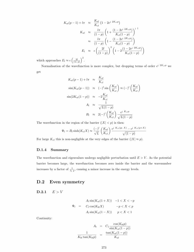
Kal(p− 1) + lπ ≈ Kal
Kcl
(1− 2e¡2Kclp
)
Kal ≈ lπ
(1− p)
(1 +
(1− 2e¡2Kclp)Kcl(1− p)
)¡1
≈ lπ
(1− p)
(1− (1− 2e¡2Kclp)
Kcl(1− p)
)
El ≈ ε
(2l
(1− p)
)2 (1− 2
(1− 2e¡2Kclp)Kcl(1− p)
)
which approaches El ≈ ε(
2l(1¡p)
)2
.
Normalisation of the wavefunction is more complex, but dropping terms of order e¡2Kclp we
get
Kal(p− 1) + lπ ≈ Kal
Kcl
sin(Kal(p− 1)) ≈ (−)l sin(
Kal
Kcl
)≈ (−)l
(Kal
Kcl
)
sin(2Kal(1− p)) ≈ −2Kal
Kcl
Al ≈ 1√L(1− p)
Bl ≈ 2(−)l
(Kal
Kcl
)e¡Kclp
√L(1− p)
The wavefunction in the region of the barrier (|X| < p) is then:
Ψl = Bl sinh(KclX) ≈ (−)l
√L
(Kal
Kcl
)e¡Kcl(p¡X) − e¡Kcl(p+X)
√(1− p)
For large Kcl this is non-negligible at the very edges of the barrier (|X| ≈ p).
D.1.4 Summary
The wavefunction and eigenvalues undergo negligible perturbation until E > V . As the potential
barrier becomes large, the wavefunction becomes zero inside the barrier and the wavenumber
increases by a factor of 11¡p , causing a minor increase in the energy levels.
D.2 Even symmetry
D.2.1 E > V
Ψl =
Al sin(Kal(1 + X)) −1 < X < −p
Cl cos(KblX) −p < X < p
Al sin(Kal(1−X)) p < X < 1
Continuity:
Al = C1cos(Kblp)
sin(Kal(1− p))1
Kbl tan(Kblp)=
tan(Kal(1− p))Kal
273

Normalisation:
|A|2 =2KalKbl cos2(Kblp)
L
Kal sin2(Kal(1− p))(2Kblp + sin(2Kblp))
+Kbl cos2(Kblp)(2Kal(1− p)− sin(2Kal(1− p)))
NBA
cot(Kal(1− p)) ≈ KblpKbl
Kal¿ 1
−(Kal(1− p)) +(2l − 1)
2π ≈ Kblp
Kbl
Kal
If we assume the barrier is low (Kal ≈ Kbl)
Kal ≈ (2l − 1)2
π
El ≈ ε(2l − 1)2
which gives the n = (2l − 1) unperturbed energies.
When the barrier rises to V = E, then Kbl becomes small enough to be negligible, and
Kal ≈ (2l − 1)2(1− p)
π
El = ε
(2l − 11− p
)2
corresponding to a slightly perturbed (p ¿ 1) energy of the n = (2l−1) solutions. For normalisation
sin(Kal(1− p)) ≈ −(−1)l
sin(2Kal(1− p)) ≈ 2KblpKbl
Kal
|Al|2 ≈ 1L
1
1 + p
(1−
(Kbl
Kal
)2)
Cl ≈ −(−1)lAl
which gives the unperturbed values when Kbl ≈ Kal. When Kbl ¿ Kal it leads to
|Al|2 ≈ 1L
(1
1 + p
)
The wavefunction in the region of the barrier approximates:
Ψ = Cl cos(KblX) ≈ Cl
D.2.2 E = V
Ψl =
Al sin(Kal(1 + X)) −1 < X < −p
Cl −p < X < p
Al sin(Kal(1−X)) p < X < 1
274

Continuity :
Al =Cl
sin(Kal(1− p))AlKal cos(Kal(1− p)) = 0
This has exact solutions
(Kal(1− p)) =(2l − 1)π
2
Kal =(2l − 1)2(1− p)
π
El = ε
(2l − 11− p
)2
Normalisation uses sin(Kal(1− p)) = −(−1)l and sin(2Kal(1− p)) = 0
Al =1√
L(1 + p)
Cl =−(−1)l
√(1 + p)
D.2.3 E < V
Ψ =
Al sin(Kal(1 + X)) −1 < X < −p
Cl cosh(KclX) −p < X < p
A1 sin(Kal(1−X)) p < X < 1
Continuity:
Al = Clcosh(Kclp)
sin(Kal(1− p))1
Kcl tanh(Kclp)= − tan(Kal(1− p))
Kal
Normalisation:
|Al|2 =2KalKcl cosh2(Kclp)
L
Kcl cosh2(Kclp)(2Kal(1− p)− sin(2Kal(1− p)))
+Kal sin2(Kal(1− p))(2Kalp− sinh(2Kalp))
NBA
When E is only slightly higher than V , these results approximate to the same results as the
approximation for NBA with E > V . These approximations match the exact solutions for E = V .
HBA
tan(Kal(1− p)) ≈ −Kal
Kcl
(1 + 2e¡2Kclp
) ¿ 1
Kal(1− p)− lπ ≈ −Kal
Kcl
(1 + 2e¡2Kclp
)
275

Kal ≈ lπ
(1− p)
(1 +
(1 + 2e¡2Kclp)Kcl(1− p)
)¡1
≈ lπ
(1− p)
(1− (1 + 2e¡2Kclp)
Kcl(1− p)
)
El ≈ ε
(2l
(1− p)
)2 (1− 2
(1 + 2e¡2Kclp)Kcl(1− p)
)
which approaches El ≈ ε(
2l(1¡p)
)2
. For normalisation, we drop terms involving e¡2Kclp and get
Kal(p− 1) + lπ ≈ Kal
Kcl
sin(Kal(p− 1)) ≈ (−)l sin(
Kal
Kcl
)
≈ (−)l
(Kal
Kcl
)
sin(2Kal(1− p)) ≈ 2Kal
Kcl
Al ≈ 1√L
1√1− p
Cl ≈ 2(−)l
√L
(Kal
Kcl
)e¡Kclp
√1− p
The wavefunction in the region of the barrier (|X| < p) is then:
Ψl = Cl cosh(KclX)
≈ (−)l
√L
(Kal
Kcl
)e¡Kcl(p¡X) + e¡Kcl(p+X)
√1− p
For large Kcl this is non-negligible at the very edges of the barrier (|X| ≈ p)
D.2.4 Summary
The even symmetry wavefunctions undergo a minor perturbation, of order p, as the barrier rises
to V = E. As the barrier rises above the energy eigenvalue, the initial peak at X = 0 becomes
a node, as the wavefunction is expelled from the potential barrier region. The energy of the lth
even eigenstate increases from the unperturbed value El = ε(2l − 1)2 to El = ε(
2l1¡p
)2
. The
final energy level, in the limit of an infinitely high barrier, becomes degenerate with the lth odd
symmetry eigenstate.
D.3 Numerical Solutions to Energy Eigenvalues
Given the dependancies of Kal, Kbl and Kcl on El and V , each of the second of the continuity
equations can be rewritten in the form f(En, V ) = 0, which defines a discrete set of eigenstates
for a given V . These eigenstates can be evaluated by numerically solving the differential equation
dEl
dV= −
(∂f
∂V
)/(∂f
∂El
)
276

with initial values given by solutions to El for the unperturbed eigenstates of V = 0 given in
Section 5.1. The solutions for El can then be used to calculate Kal and so plot the wavefunction
itself. Numerical solutions to these equations were evaluated using the MATLAB[MAT] analysis
100
101
102
103
0
5
10
15
20
25
30
35
40
Potential Barrier Height
Ene
rgy
Eig
enva
lues
Figure D.1: First six energy eigenvalues with potential barrier
package, and setting ε = L = 1, p = 0.01 The results are shown in Figures D.1,D.2 and D.3.
Figure D.1 shows the changes in the eigenvalues of the first three (odd and even symmetry)
pairs of eigenstates as the barrier height increases. The eigenvalues pass continuously from the
V = 0 values, through V = E, to the V À E values, becoming degenerate only in the limit
of the infinitely high barrier. Figure D.2 shows the changes in the wavefunction of the first and
third even symmetry eigenstates, with barrier heights starting at twice the energy eigenvalue. The
eigenstates clearly develop a node in the center, shortening their wavelengths, until they reach the
same wavelength as the corresponding odd symmetry state. Finally, in the limit of the infinite
potential barrier the odd and even symmetry states differ only by a change of sign at they pass
through the origin, shown in Figure D.3
277

−1 −0.8 −0.6 −0.4 −0.2 0 0.2 0.4 0.6 0.8 10
0.1
0.2
0.3
0.4
0.5
0.6
0.7
0.8
0.9
1
Position
Wav
efun
ctio
n
−1 −0.8 −0.6 −0.4 −0.2 0 0.2 0.4 0.6 0.8 1−1
−0.8
−0.6
−0.4
−0.2
0
0.2
0.4
0.6
0.8
1
Figure D.2: Perturbation of Even Symmetry Eigenstates
−1 −0.8 −0.6 −0.4 −0.2 0 0.2 0.4 0.6 0.8 1−1
−0.8
−0.6
−0.4
−0.2
0
0.2
0.4
0.6
0.8
1
Wav
efun
ctio
n
Position−1 −0.8 −0.6 −0.4 −0.2 0 0.2 0.4 0.6 0.8 1
−1
−0.8
−0.6
−0.4
−0.2
0
0.2
0.4
0.6
0.8
1
Wav
efun
ctio
n
Position
Figure D.3: Degeneracy of Even and Odd Symmetry Eigenstates
278

Appendix E
Energy of Perturbed Airy
Functions
The insertion of shelves at height h into the wavefunction of a quantum weight will cause a
perturbation of the energy eigenvalues. Due to the nature of the Airy functions, it is not possible
to calculate the effect of this perturbation exactly. However, it can be estimated for two extremes,
and be shown to involve negligible energy changes for high quantum numbers. It is argued that it
is reasonable to assume that there is also negligible energy changes between the two extremes.
This is based upon calculations in [NIS] for the quantum state of a particle in a linear potential
between two barriers. We will calculate the effect of inserting a potential barrier for high quantum
numbers n, where the shelf height is large and small in comparison with the characteristic height of
the wavefunction −anH. The unperturbed energy of the state is En = −anMgH. We will always
use the asymptotic approximation an = − (3πn2
)2/3.
Large Shelf Height
If the shelf is inserted at a height h À −anH then there is negligible perturbation of the wave-
function, as the potential changes only in a region where the wavefunction is negligibly small. The
final energy is therefore approximately the same as the unperturbed energy:
E(1)n =
(3πn
2
)2/3
MgH
Small Shelf Height
If the shelf is inserted at a height h ¿ −anH, the wavefunction is split into two, above and below
the shelf. We will start by assuming that the shelf is inserted at a node, and that m nodes are
above the shelf height (see Figure 5.5). The number of nodes below the shelf height is given by
k = n−m, and the shelf height is h = (am − an)H.
279

The low shelf height is equivalent to the assumption that k ¿ n. There are two subcases,
depending upon whether k itself is large or small.
If k is small, then m ≈ n and there is negligible probability of the weight being located below
the shelf, and we only need to consider the wavefunction above. This is the same as an unperturbed
wavefunction with m nodes, raised by a height h, and so will have an energy
E(2)m = −amMgH + Mgh
= −anMgH
= En
If 1 ¿ k ¿ n we need to estimate the energy of the wavefunction above and below the barrier.
Above the barrier, we again have a wavefunction with energy E(2)m =
itJ -75.cane (b)84253(as)-254(he)-2537.16 TDh

of the potential barrier will then have negligible effect upon the energy levels of the high quantum
number states.
281

Appendix F
Energy Fluctuations
We suppose that the expansion of the gas, described in Section 6.2 takes places in n steps, and
after each step the gas is allowed to thermalise through interactions with an environment. This
thermalisation randomises the individual state of the gas from step to step.
The energy transferred by the i0th state, on the m0th step is denoted by δEim and the probability
of the gas being in the i0th state, on the m0th step is pim. Clearly∑
i pim = 1. The randomisation of
the state between steps means that the probabilities at different steps can be treated as statistically
independant.
We describe the ordered set of states that the system passes through on a given expansion by
the array α = (ijk . . .), which means the system is in the i0th state on the first step, j0th state on
the second step, etc. We also write this as α1 = i, α2 = j or α = (α1α2 . . .). The probability of α
occurring is given by
Pα =∏
m=1,n
pαmm
∑α
Pα =∑
α1,α2,...
( ∏m=1,n
pαmm
)= 1
and the energy transferred on such an expansion is
Eα =∑m
δEαmm
We also need to note the following identities
∑α1,α2,...
( ∏m=1,n
pαmmf(αk)
)=
∑αk
pαkkf(αk)
∑α1,α2,...
( ∏m=1,n
pαmmf(αk, αl)
)=
∑αk,αl
pαkkpαllf(αk, αl)
etc.
We can now write the following results
282

Mean energy transfer and fluctuation on m0th step:
〈δEm〉 =∑
i
pimδEim
⟨δE2
m
⟩=
∑
i
pim (δEim)2
Mean energy transfer and fluctuation of the overall expansion is:
〈E〉 =∑α
∏
l=1,n
pαll
(∑m
δEαmm
)=
∑m
(∑αm
pαmmδEαmm
)
=∑
m=1,n
〈δEm〉
〈E〉2 =∑m
〈δEm〉2 + 2∑
l<m
〈δEl〉 〈δEm〉
⟨E2
⟩=
∑α
∏
l=1,n
pαll
(∑m
δEαmm
)2
=∑α
∏
k=1,n
pαkk
∑
l,m
δEαllδEαmm
=∑m
(∑αm
pαmm (δEαmm)2)
+ 2∑
l<m
∑αm,αl
pαmmpαllδEαmmδEαll
=∑m
⟨δE2
m
⟩+ 2
∑
l<m
〈δEl〉 〈δEm〉⟨E2
⟩− 〈E〉2 =∑
m=1,n
(⟨δE2
m
⟩− 〈δEm〉2)
For the expansions in Section 6.2, we have⟨δE2
m
⟩ − 〈δEm〉2 = 2 〈δEm〉2. We may therefore
introduce the following inequalities:
⟨E2
⟩− 〈E〉2 ≤ 2n 〈δEmax〉2
〈E〉2 ≥ (n 〈δEmin〉)2
and prove our required result that⟨E2
⟩− 〈E〉2〈E〉2 ≤ 2
n
( 〈δEmax〉〈δEmin〉
)2
The ratio hδEmaxihδEmini approaches Pmax
Pmin, where Pm = ∂Em
∂X is the generalised pressure, as the size
of the step reduces, and so becomes independant of n. As n = t/τθ, where τθ is a characteristic
thermal relaxation time, and t is the length of time of the expansion, the size of fluctuations in the
total energy transfer can be made negligible if the expansion takes place sufficiently slowly with
respect to τθ.
It should be clear that the result obtained here is not the same as, although it is similar to, the
usual fluctuation formula. The usual formula refers to the deviation from the mean value of the
thermodynamic variable at a given time, and is reciprocally related to the number of constituents
of the system. The formula here refers to potentially large fluctuations at any particular moment,
283

for systems which may have only a few constituents, but which, when integrated over a significant
period of time, still leads to negligible long term fluctuations.
284

Appendix G
Free Energy and Temperature
The free energy, F is only one of a number of thermodynamics potentials that may be associated
with a system. For example, we can also use the energy E, Gibbs function G or enthalpy H,
defined by
E
F = E − TS
G = E − TS + PV
H = E + PV
to describe the behaviour of a system. These terms can them be generalised even further, when
the number of particles is allowed to vary. The choice of which thermodynamic potential to use
entirely is a question of which constraints are acting upon the system, or which pair of the variables
S, T , P and V are controlled.
In Section 7.1, the significance of F and from that S was derived from the work that can
be extracted from an isothermal expansion of a system. In terms of classical thermodynamics
potentials, this is derived from the infinitesimal relationships
dF = dE − TdS − SdT
and the general relationship for heat and work acting upon a system
dE = TdS − PdV
which is equivalent to the statistical mechanical relationship
dE =∑
i
Eidpi +∑
i
pidEi
This gives
dF = −SdT − PdV
285

and clearly, if the temperature is held fixed
dF = −PdV
so the change in free energy is equal to the negative of the work extracted from the system,
dW = PdV .
Now, if the temperature is not held fixed, then we clearly have
dF + dW = −SdT
If we can interpret the work as being the gain in free energy of a second system (which has no
change in entropy), such as a raised weight, we can express this equation as being a net gain in
free energy ∆F = dF + dW, of a closed system, when a quantity of entropy S is taken through a
temperature difference ∆T = dT . We will express this as
∆F = −S∆T (G.1)
and refer to this as the characteristic equation for free energy in the presence of a temperature
differences.
Adiabatic expansion The derivation above is essentially based upon the adiabatic (essentially
isolated) expansion of a gas. If we take a gas in essential isolation, and extract work from it’s
expansion, the free energy before and after is given by
F1 = E1 − T1S1
F2 = E2 − T2S2
As the expansion is reversible but thermally isolated we have ∆W = E1−E2 and S2 = S1 = S.
This gives
∆F = F2 − F1
= −∆W − (T2 − T1)S
∆F + ∆W = −S∆T
Carnot Cycle The Carnot heat engine operates by drawing energy in the form of heat Q1
from a heat bath at temperature T1, extracting W as work, and depositing Q2 in a heat bath
at temperature T2. The usual means of achieving this would be to have gas initially in contact
with the heat bath T1. This is isothermally expanded, drawing the Q1 out as work. The gas is
then removed from contact with the heat bath, and adiabatically expanded, again extracting work,
until it’s temperature falls to T2. It is then placed in contact with the T2 heat bath, isothermally
286

compressed, depositing the Q2 heat, and is then isolated again, and adiabatically compressed
further until it returns to it’s initial volume, at which point, on a reversible cycle, it will have risen
back to temperature T2.
For a reversible process the entropy loss from the T1 heat bath must match the gain from the
T2 heat bath, so
S =Q1
T1=
Q2
T2
and conservation of energy is
Q1 = Q2 + W
This is usually rearranged to give the Carnot efficiency
W
Q1= 1− T2
T1
However, there is an alternative way of expressing this
W = −S (T2 − T1)
which is again the characteristic equation G.1 for free energy in the presence of two different
temperatures.
Entropy Engine The two previous examples can be regarded as equations about the movement
of energy between, or within, systems, rather than an equation about the gain in free energy from
moving entropy between different temperatures. We will now demonstrate a system, based upon
the Szilard Engine, and with some similarities to the heat engines described in Chapter 8, but
which produces this characteristic equation without any energy changes taking place anywhere.
This makes it very clear that the gain in free energy is actually a consequence of the transferral of
entropy between temperatures.
First we start with two Szilard boxes, each containing a single atom, and initially of length L.
The boxes are initially at temperatures T1 and T2, but are thermally isolated. A partition is raised
in the centre of the first box, dividing the one atom gas into left and right subensembles, and a
piston is inserted between them.
Now, however, we modify the behaviour of the box, as shown in Figure G.1. The piston is
constrained so that it cannot move to the right, even when the gas is located to the left. If the gas
is on the right, the piston moves to the left, as before. However, regardless of the location of the
gas, the right most wall of the box starts to move to the left, at the same rate as a left-moving
piston would. When the wall of the box reaches the initial center, it stops. If the gas was initially
located to the left of the partition, the right wall simply moves in through empty space on the right,
until it comes against the piston, still in the center. If, on the other hand, the gas was initially
located to the right, the piston and wall move leftwards together. As long as this movement is
sufficiently slow, any work done upon the piston would be matched by work done by the wall.
In effect, no work is done upon the gas at all, as the right subensemble keeps the same volume
287

Figure G.1: The Entropy Engine
throughout. At the end of this process, the wall is in the initial center, and the piston is against
the left wall. The initially left and right gas subensembles are now entirely overlapping.
The remarkable consequence of this is that we have compressed the gas to exactly half it’s
volume, but without performing any work upon it, or changing it’s energy in any other way.
We have succeeded in this by increasing the entropy of the piston, which is now in a mixture of
being on the left or the right. This effect is possible only from statistical mechanics: there is
no equivalent process in phenomenological thermodynamics by which such a compression can be
achieved without any flow of energy.
We now remove the piston states from the ends of the first box and insert them in the corre-
sponding ends of the second. We can now perform the same operation on the second Szilard box,
in the reverse direction. The second gas expands to twice it’s volume, while the piston is restored
to it’s initial state. Again, there is no contact with a heat bath, no work is extracted from the gas,
and it’s internal energy is constant throughout.
It is clear that we can continue this process indefinitely, compressing the first gas to as small
a fraction of it’s initial volume as we like, without ever performing any work upon it. However,
the cost is that we must proportionately increase the volume occupied by the second. The only
quantity that is transferred between the two systems is the mixing entropy of the piston, S = k ln 2.
However, by compressing the first gas we increase it’s free energy by kT1 ln 2, and by expanding
288

the second gas, reduce it’s free energy by kT2 ln 2. The net change in free energy is
∆F = k ln 2(T1 − T2)
= −S∆T
which corresponds to the entropy being transferred through the temperature difference ∆T =
T2−T1 This provides an ’engine’ by which the free energy of a system can be increased indefinitely,
by reversibly moving entropy between parts of the system at different temperatures, yet without
any energy flow taking place.
Of course, when we attempt to extract this free energy by, for example, isothermally restoring
the system to it’s initial configuration, we simply recover the Carnot cycle efficiency. Although
this process produces the characteristic equation G.1 for the free energy change in the presence
of different temperatures, it should be clear that it’s physical basis is a purely statistical mechan-
ical effect, and quite different to the more commonly encountered manifestation in the adiabatic
expansion and Carnot Cycle.
289

Appendix H
Free Energy and Non-Equilibrium
Systems
In Section 7.1 the free energy of a system in a canonical thermodynamical state ρ = 1Z e¡ H
kT was
derived in terms of it’s partition function Z = Tr[e¡ H
kT
]=
∑i e¡ Ei
kT as F = −kT ln Z.
When the Hilbert space is split into subspaces with partition functions Za =∑
i‰a e¡ EikT , the
equilibrium probability of the density matrix being in the subspace is
pa =∑
i‰a
pi =∑
i‰a e¡ EikT
∑i e¡ Ei
kT
=Za
Z
From this we can express the free energy of a density matrix in equilibrium in the subspace by
Fa = F − kT ln pa
When the Hilbert space is divided into several orthogonal subspaces, so that Z =∑
α Zα, we
have
F =∑α
pαFα + kT∑α
pα ln pα
= −kT ln
(∑α
e¡ FαkT
)
and also
pa =e¡ Fa
kT
∑α e¡ Fα
kT
The equilibrium density matrix may be expressed as
ρ =∑α
pαρα
=1Z
∑α
e¡ FakT ρα
290

Note that this is expressed in terms of the free energies of the subensembles, rather than the
energies of the microstates.
We now wish to consider what happens when an density matrix is composed of the same equi-
librium subensembles ρα but for which the mixing probabilities p0α are not in thermal equilibrium1
ρ0 =∑α
p0αρα
We know the entropy of this matrix from the mixing equation
S0 =∑α
p0αSα − k
∑α
p0α ln p0
α
However, it may seem unclear whether the free energy is at all meaningful in this situation. We
cannot simply use F as the equations would not agree. At the same time, there is a well defined
temperature associated with the system. We need to develop a well defined generalisation of the
equilibrium equations above.
We are going to proceed by proposing a non-equilibrium version of the partition function
Z 0 =∑α
Dαe¡ FakT
where the Dα are a set of factors which determine the extent to which the system is out of
equilibrium. If all Dα = 1 then the system is in equilibrium. We define the Da from the constraint∑
α p0α ln Dα = 0 to give
kT ln Da = (Fa + kT ln p0a)−
∑α
p0α (Fα + kT ln p0
α)
which allows us to write
p0a =
1Z 0 Dae¡ Fa
kT
ρ0 =1Z 0
∑α
Dαe¡ FakT ρα
in analogy to our equilibrium equations.
We would now like to express the non-equilibrium free energy as just F 0 = −kT ln Z 0. Our
primary justification for believing this is because the mean energy E, the non-equilibrium entropy
S0 and the subensemble temperature T can be shown to be related by
E − TS0 = −kT ln Z 0
which is precisely the relationship we would like a free energy to fulfil. However, the operational
definition free energy, that makes it a useful to use, is that it corresponds to the work required to1We may imagine that each of the subspaces corresponds to a separate ’box’, between which transitions are
inhibited. We can then easily prepare a system in which the ’boxes’ are each in equilibrium with some heat bath,
but the probabilities of the ’boxes’ being occupied are not in an equilibrium. As long as the thermal relaxation time
for transitions between boxes is very large, this will be stable.
291

put the system into some reference state, by an isothermal procedure. We must show the work
required to change the state matches the change in F 0. To be sure that this is valid, the final
reference state should be one in which the subensembles occur with equilibrium probability.
Let us start with a particularly simple example, consisting of Szilard box and a piston system.
It is the piston system that we are going to focus upon. The piston system is initially in one of two
states, which have the same internal entropies SP , energies Ep and are in equilibrium temperature
T, which for simplicity will be the same temperature as the Szilard box. The ’internal’ free energy
of the piston states are therefore Fp = Ep − TSp. In a ’thermal equilibrium’ each of the piston
states would be equally likely and in an equilibrium mixture of piston states, the free energy would
be F = Fp − kT ln 2.
If we placed two piston states in opposite ends of the Szilard box, and compress the gas until
each piston state was found in the center of the box, the isothermal work required is just kT ln 2.
The piston is now no longer in the mixture, and has free energy FP . When the piston is removed,
the gas expands to refill the entire box. This allows us to isothermally put the equilibrium state
into a reference state, with a work requirement of kT ln 2. We could also reverse the procedure, and
allow the piston reference state to expand into an equilibrium mixture, extracting kT ln 2 work.
We now consider what happens if the initial piston states occur with the more general proba-
bilities of p and 1− p. We will again place the two piston states at each end of the box, but now
we compress the two sides by different amounts, so the piston ends up in some position Y , not
necessarily the center. If the piston is on the left, with probability p, we allow it to compress the
gas to the right of Y . This requires a work of kT ln(
21¡Y
). If the piston is on the right, with
probability (1− p), the gas is compressed to the left of Y, and the work required is kT ln(
21+Y
).
The mean work requirement is therefore
W
kT= p ln
(2
1− Y
)+ (1− p) ln
(2
1 + Y
)
This has its smallest value when p =(
1¡Y2
)and therefore
W = −kT (p ln p + (1− p) ln(1− p))
This leaves the piston at position Y = (1 − 2p), with the one atom gas located to the left of
the piston, with probability(
1+Y2
)and to the right with probability
(1¡Y
2
). Had we inserted a
partition into the box at position Y , we would have precisely these probabilities for the location
of the one atom gas. The piston can therefore be reversibly removed from the box. Had the
compression of the gas left the piston at some other value of Y 0, removing and reinserting the
piston at Y 0 would lead to a rearrangement of the probabilities of the one atom gas. This would
not be a reversible procedure. This demonstrates that the work requirement to reversibly put the
non-equilibrium mixture of piston states into the reference state is exactly −T∆S, where ∆S is
just the mixing entropy of the non-equilibrium state.
We consider this to be the required generalisation of isothermal compression. For the change
in free energy to be equal to the work done, the initial free energy must be
292

F 0 = Fp + kT (p ln p + (1− p) ln(1− p))
This can be readily generalised to a situation with many different subensembles and with
different free energies in each subensemble, but with all subensembles at the same temperature2
to yield
F 0 =∑α
p0α (Fα + kT ln p0
α)
= E − TS0
= −kT ln Z 0
which is the desired result, and justifies the form of the non-equilibrium partition function.
With regard to the other relationships involving the free energy, we find these generalise to
F 0 = −kT ln
(∑α
Dαe¡ FαkT
)
p0a =
DaZa
Z 0
Fa = F 0 − kT ln(
p0a
Da
)
These relations are less useful than they might appear. We have justified the existence of a
free energy for situations where a system is in a stable, non-equilibrium state, but has a well
defined temperature. However the dependance upon the values of Dα makes the non-equilibrium
partition function of limited value when these are changeable (unless they can be constrained to
be changeable in a well defined way eg. when the system is not isolated, the Dα will approach
1, typically with an exponential decay, and over a time period of the same order as the thermal
relaxation time). It should be noted, however, that the non-equilibrium state will have a higher
free energy than the equivalent equilibrium state. As the system approaches equilibrium this extra
free energy will be lost in the process of thermalisation.
2If the internal states of the piston are assumed to be thermally isolated from the Szilard box, then the com-
pression may take place at a different temperature. While this complicates the process, it will still be consistent
with the free energy defined here, taking into account the results of Appendix G, where there is more than one
temperature present.
293
Bibliography
[AA98] Y Aharanov and J Anandan. Meaning of the density matrix. 1998. quant-ph/9803018.
[AC95] C Adami and N J Cerf. Negative entropy and information in quantum mechanics. 1995.
quant-ph/9512022.
[AC97] C Adami and N J Cerf. Quantum mechanics of measurement. Phys Rev A, 1997.
quant-ph/9605002.
[AE74] L Allen and J H Eberly. Optical Resonance and Two-Level Atoms. 1974.
[Alb92] D Z Albert. Quantum Mechanics and Experience. Harvard University Press, 1992.
[Alb94] D Z Albert. The foundations of quantum mechanics and the approach to thermody-
namic equilibrium. Brit J Phil Sci, 45:669–677, 1994.
[AS70] M Abramowitz and I A Stegun. Handbook of Mathematical Functions. Dover, 1970.
[AV96] Y Aharanov and L Vaidman. About position measurements which do not show the
bohmian particle position. In [CFG96], pages 141–154, 1996.
[BBBH97] S L Braunstein, D Bruss, V Buzek, and M Hillery. Phys Rev A, 56(5):3446–3452, 1997.
[BBC+93] C H Bennett, G Brassard, C Crepeau, R Jozsa, A Peres, and W K Wootters. Physical
Review Letters, 70:1895–1899, 1993.
[BBM00] C M Bender, D C Brody, and B K Meister. Quantum-mechanical Carnot engine. 2000.
quant-ph/0007002.
[BDE98] V Buzek, R Derka, and A K Ekert. Universal algorithm for optimal estimation of
quantum states from finite ensembles via realizable generalised measurement. Phys
Rev Lett, 80(8):1571–1575, 1998.
[BDF+99] C H Bennett, D P DiVincenzo, C A Fuchs, T Mor, E Rains, P W Shor, J A Smolin,
and W K Wootters. Quantum non-locality without entanglement. Physical Review A,
59:1070, 1999. quant-ph/9804053.
[BDH+93] M Brune, L Davidovich, S Haroche, A Maali, and J M Raimond. Quantum switches
and nonlocal microwave fields. Physical Review Letters, 71(15):2360–2363, 1993.
294

[BDH+94] M Brune, L Davidovich, S Haroche, J M Raimond, and N Zagury. Teleportation of an
atom state between two cavities using nonlocal microwave fields. Physical Review A,
50(2):R895–R898, 1994.
[Bel80] J S Bell. de Broglie-Bohm, delayed-choice double-slit experiment, and density matrix.
International Journal of Quantum Chemistry, pages 155–159, 1980. in [Bel87].
[Bel87] J S Bell. Speakable and unspeakable in quantum mechanics. Cambridge University
Press, 1987.
[Ben73] C H Bennett. The logical reversibility of computation. IBM J Res Develop, 17:525–532,
1973.
[Ben82] C H Bennett. The thermodynamics of computation - a review. Int J Theor Phys,
21:905–940, 1982. Reprinted in [LR90].
[BG99a] A Bassi and G Ghirardi. About the notion of truth in the decoherent histories approach:
a reply to Griffiths. 1999. quant-ph/9912065.
[BG99b] A Bassi and G Ghirardi. Can the decoherent histories description of reality be consid-
ered satisfactory? Phys Lett A, 257:247–263, 1999.
[BG99c] A Bassi and G Ghirardi. Decoherent histories and realism. 1999. quant-ph/9912031.
[BGL95] P Busch, M Grabowski, and P J Lahti. Operational Quantum Physics. Springer, 1995.
[BH84] D Bohm and B J Hiley. Foundations of Physics, 14:255–274, 1984.
[BH87] D Bohm and B J Hiley. An ontological basis for quantum theory: I non-relativistic
particle systems. Physics Reports, 144:323–348, 1987.
[BH93] D Bohm and B J Hiley. The Undivided Universe. Routledge, 1993.
[BH96a] D Bohm and B J Hiley. Statistical mechanics and the ontological interpretation. Foun-
dations of Physics, 26(6):823–846, 1996.
[BH96b] V Buzek and M Hillery. Quantum copying: beyond the no-cloning theorem. Phys Rev
A, 54(3):1844–1852, 1996.
[BH00] M Brown and B J Hiley. Schrodinger revisited: an algebraic approach. 2000. quant-
ph/0005026.
[BHK87] D Bohm, B J Hiley, and P N Kaloyerou. An ontological basis for quantum theory II:
A causal interpretation of quantum fields. Phys Rep, 144(6):349–375, 1987.
[BKV97] S Bose, P L Knight, and V Vedral. Physical Review A, 56:4175–4186, 1997.
[Boh51] D Bohm. Quantum Theory. Prentice-Hall, 1951.
295


[CHM00] R E Callaghan, B J Hiley, and O J E Maroney. Quantum trajectories, real, surreal or
an approximation to a deeper process? 2000. quant-ph/0010020.
[CJ63] F W Cummings and E T Jaynes. Proc IEEE, 51:89, 1963.
[CN01] I L Chuang and M A Nielsen. Quantum Computation and Quantum Information.
Cambridge, 2001.
[CP94] J I Cirac and A S Parkins. Schemes for atomic state teleportation. Physical Review A,
50(6):R4441–R4444, 1994.
[Cun98] M O T Cunha. What is surrealistic about Bohm trajectories? 1998. quant-ph/9809006.
[Dav78] E B Davies. Information and quantum measurement. IEEE Transactions on Informa-
tion Theory, IT-24(5):596–599, 1978.
[dBT74] O Costa de Beauregard and M Tribus. Information theory and thermodynamics. Phys
Acta, 47:238–247, 1974. Reprinted in [LR90].
[DD85] K G Denbigh and J S Denbigh. Entropy in Relation to Incomplete Knowledge. Cam-
bridge University Press, 1985.
[Deu85] D Deutsch. Quantum theory, the Church-Turing principle and the universal quantum
computer. Proc R Soc Lond A, 400:97–117, 1985.
[Deu89] D Deutsch. Quantum computational networks. Proc R Soc Lond A, 425:73–90, 1989.
[Deu97] D Deutsch. The Fabric of Reality. Penguin, 1997.
[DFGZ93] D Durr, W Fusseder, S Goldstein, and N Zanghi. Comment on surrealistic Bohm
trajectories. Z Naturforsch, 48a:1261–1262, 1993.
[DG73] B DeWitt and N Graham, editors. The Many-Worlds Interpretation of Quantum Me-
chanics. Pirnceton University Press, 1973.
[DHK87] C Dewdney, P Holland, and Kyprianidis. Journal of Physics A, 20:4717–4732, 1987.
[DHP79] C Dewdney, B J Hiley, and C Philippidis. Quantum interference and the quantum
potential. Il Nuovo Cimento, 52B:15–28, 1979.
[DHS93] C Dewdney, L Hardy, and E J Squires. How late measurements of quantum trajectories
can fool a detector. Phys Lett A, 184(1):6–11, 1993.
[DL94a] C Dewdney and M M Lam. The Bohm approach to cavity quantum scalar field dy-
namics. Part I the free field. Found Phys, 24(1):3–27, 1994.
[DL94b] C Dewdney and M M Lam. The Bohm approach to cavity quantum scalar field dy-
namics. Part II the interaction of the field with matter. Found Phys, 24(1):29–60,
1994.
297

[EN98] J Earman and J D Norton. Exorcist XIV: The Wrath of Maxwell’s Demon. Part I:
From Maxwell to Szilard. Hist Phil Mod Phys, pages 435–471, 1998.
[EN99] J Earman and J D Norton. Exorcist XIV: The Wrath of Maxwell’s Demon. Part II:
From Szilard to Landauer and beyond. Stud Hist Phil Mod Phys, 30:1–40, 1999.
[ESSW92] B G Englert, M O Scully, G Sussmann, and H Walther. Surrealistic Bohm trajectories.
Z Naturforsch, 47A:1175–1186, 1992.
[ESSW93] B G Englert, M O Scully, G Sussmann, and H Walther. Reply to comment on surreal-
istic Bohm trajectories. Z Naturforsch, 48a:1263–1264, 1993.
[ESW91] B G Englert, M O Scully, and H Walther. Nature, 351:111, 1991.
[Fah96] P N Fahn. Maxwell’s demon and the entropy cost of information. Foundations of
Physics, 26(1):71–93, 1996.
[Fey63] R P Feynman. The Feynman Lectures on Physics, volume 1. 1963.
[Fey66] P K Feyerabend. On the possibility of perpetual motion of the second kind. In P K Fey-
erabend and G Maxwell, editors, Mind, Matter and Method, pages 409–412. University
of Minnesota, 1966.
[Fey93] P K Feyerabend. Against Method. Verso, third edition, 1993.
[Fey99] R P Feynman. Lectures on Computation. Penguin, 1999.
[Fis25] R A Fisher. Proc Cambridge Philos Soc, 22:700, 1925.
[Fri88] B R Frieden. Applications to optics and wave mechanics of the criterion of maximum
cramer-rao bound. Journal of Modern Optics, 35(8):1297–1316, 1988.
[Fri89] B R Frieden. Fisher information as the basis for the Schrodinger wave equation. Amer-
ican Journal of Physics, 57(11):1004–1008, 1989.
[Fri98] B R Frieden. Physics from Fisher information. Cambridge University Press, 1998.
[FS95] B R Frieden and B H Soffer. Langrangians of physics and the game of Fisher-information
transfer. Physical Review E, 52(3):2274–2286, 1995.
[Gab64] D Gabor. Light and information. Progress in Optics, 1:111–153, 1964. Based on lectures
delivered in 1951. Reprinted in [LR90].
[GM97] N Gisin and S Massar. Optimal quantum cloning machines. Phys Rev Lett, 79(11):2153–
2156, 1997.
[GP99] N Gisin and S Popescu. Spin flips and quantum information for anti-parallel spins.
Phys Rev Lett, 83(2):432–435, 1999. quant-ph/9901072.
298

[Gri84] R B Griffiths. Consistent histories and the interpretation of quantum mechanics. J
Stat Phys, 36:219–271, 1984.
[Gri93] R B Griffiths. The consistency of consistent histories: a reply to d’Espagnat. Found
Phys, 23(12):1601–1610, 1993.
[Gri94] R B Griffiths. A consistent history approach to the logic of quantum mechanics. In K V
Lasurikainen, C Montonen, and K Sunnarborg, editors, Symposium on the Foundations
of Modern Physics, 1994.
[Gri96] R B Griffiths. Consistent histories and quantum reasoning. Phys Rev A, 54(4):2759–
2774, 1996.
[Gri98] R B Griffiths. Choice of consistent family and quantum incompatibility. Phys Rev A,
57(3):1604–1618, 1998.
[Gri99] R B Griffiths. Bohmian mechanics and consistent histories. 1999. quant-ph/9902059.
[Gri00] R B Griffiths. Consistent quantum realism: a reply to Bassi and Ghirardi. 2000.
quant-ph/0001093.
[Gru99] J Gruska. Quantum Computing. McGraw-Hill, 1999.
[Hal00] M J W Hall. Comment on ”Conceptual inadequacy of the Shannon information ...” by
C Brukner and A Zeilinger. 2000. quant-ph/0007116.
[Hei58] W Heisenberg. Physics and Philosophy. Harper and Row, 1958.
[HH96] R Horodecki and M Horodecki. Physical Review A, 54:1838–1843, 1996.
[HJS+96] P Hausladen, R Josza, B Schumacher, M Westmoreland, and W K Wootters. Phys Rev
A, 54:1869, 1996.
[HM99] B J Hiley and O J E Maroney. Quantum state teleportation understood through the
Bohm interpretation. Found Phys, 29(9), 1999.
[HM00] B J Hiley and O J E Maroney. Consistent histories and the Bohm approach. 2000.
quant-ph/0009056.
[Hol88] P R Holland. Physical Reports, 169:293, 1988.
[Hol93] P R Holland. The Quantum Theory of Motion. Cambridge, 1993.
[HPMZ94] J J Halliwell, J Perez-Mercader, and W H Zurek, editors. Physical Origins of Time
Asymmetry. Cambridge, 1994.
[Jay79] E T Jaynes. Where do we stand on maximum entropy? In [LT79], 1979.
299

[JB72] J M Jauch and J G Baron. Entropy, information and Szilard’s paradox. Helv Phys
Acta, 47:238–247, 1972. Reprinted in [LR90].
[Joz96] R Jozsa. Quantum algorithms and the Fourier transform. In E Knill, R LaFlamme,
and W Zurek, editors, Quantum Coherence and Decoherence, 1996.
[Joz97] R Jozsa. Entanglement and quantum computation. In S Huggett, L Mason, K P Todd,
S T Tsou, and N M J Woodhouse, editors, Geometric Issues in the Foundations of
Science. Oxford University Press, 1997. quant-ph/9707034.
[JS94] R Jozsa and B Schumacher. A new proof of the quantum noiseless coding theorem. J
Mod Optics, 41(12):2343–2349, 1994.
[Kal94] P N Kaloyerou. The causal interpretation of the electromagnetic field. Phys Rep,
244:287–358, 1994.
[Kho73] A S Kholevo. Bounds for the quantity of information transmitted by a quantum com-
munication channel. Problems in Information Transmission, 9:177–183, 1973.
[Kho98] A S Kholevo. IEEE Trans Info Theory, 44:269, 1998.
[Kul59] S Kullback. Information Theory and Statistics. Wiley, 1959.
[Lan61] R Landauer. Irreversibility and heat generation in the computing process. IBM J Res
Dev, 5:183–191, 1961. Reprinted in [LR90].
[Lan92] R Landauer. Information is physical. In Workshop on Physics and Computation,
PhysComp’92. IEEE Computer Society, 1992.
[Lef95] H S Leff. Thermodynamic insights from a one-atom gas. Am J Phys, 63(10):895–905,
1995.
[LL77] L D Landau and E M Lifschitz. Quantum Mechanics. Pergamon, third edition, 1977.
[LPT98] J I Latorre, P Pascual, and R Tarrach. Minimal optimal generalized quantum mea-
surements. Phys Rev Lett, 81(7):1351–1354, 1998.
[LPTV99] J I Latorre, P Pascual, R Tarrach, and G Vidal. Optimal minimal measurements of
mixed states. Phys Rev A, 60(1):126–135, 1999.
[LR90] H S Leff and A F Rex, editors. Maxwell’s Demon. Entropy, Information, Computing.
Adam Hilger, 1990.
[LR94] H S Leff and A F Rex. Entropy of measurement and erasure: Szilard’s membrance
model revisited. Am J Phys, 62(11):994–1000, 1994.
[LT79] R D Levine and M Tribus, editors. The Maximum Entropy Formalism. MIT, 1979.
300

[LTV98] M Li, J Tromp, and P Vitanyi. Reversible simulation of irreversible computation by
pebble games. Physica D, 120(1-2):168–176, 1998. quant-ph/9703009.
[Lub87] E Lubkin. Keeping the entropy of measurement: Szilard revisited. Int J Theor Phys,
26:523–535, 1987. Reprinted in [LR90].
[LV96] M Li and P Vitanyi. Reversibility and adiabatic computation: Trading time and space
for energy. Proc R Soc Lond A, 452:769–789, 1996.
[Mar01] O J E Maroney. Sameness and oppositeness in quantum information. In Proc ANPA22,
2001.
[Mas00] S Massar. Collective versus local measurements on two parallel or antiparallel spins.
2000. quant-ph/0004035.
[MAT] Matlab. www.mathworks.com.
[Mes62] A Messiah. Quantum Mechanics, volume II. Wiley, 1962.
[Mou97] M H Y Moussa. Physical Review A, 55:3287–3290, 1997.
[MP95] S Massar and S Popescu. Optimal extraction of information from finite quantum en-
sembles. Phys Rev Lett, 74(8):1259–1263, 1995.
[MW95] L Mandel and E Wolf. Optical Coherence and Quantum Optics. Cambridge University
Press, 1995.
[Neu55] J von Neumann. Mathematical Foundations of Quantum Mechanics. Princeton Uni-
versity Press, 1955.
[NIS] NIST. Digital library of mathematical functions. http://dlmf.nist.gov.
[Par89a] M H Partovi. Irreversibility, reduction and entropy increase in quantum measurements.
Phys Lett A, 137(9):445–450, 1989.
[Par89b] M H Partovi. Quantum thermodynamics. Phys Lett A, 137(9):440–444, 1989.
[Pen70] O Penrose. Foundations of Statistical Mechanics. Pergamon, 1970.
[Per80] A Peres. Measurement of time by quantum clocks. Am J Phys, 48(7):552–557, 1980.
[Per90] A Peres. Neumark’s theorem and quantum inseparability. Found Phys, 20(12):1441–
1453, 1990.
[Per93] A Peres. Quantum Theory: Concepts and Methods. Kluwer, 1993.
[Pop56] K R Popper. Quantum Theory and the Schism in Physics, chapter 1, pages 104–118.
Rowman and Littlefield, 1956.
301

[Pop57] K R Popper. Irreversibility, or entropy since 1905. Brit J Phil Sci, 8:151–155, 1957.
[Pop74] K R Popper. Autobiography. In P A Schilpp, editor, The Philosophy of Karl Popper,
pages 124–133. Open Court, 1974.
[Pop94] S Popescu. Physical Review Letters, 72:797–799, 1994.
[Red87] M L G Redhead. Incompleteness, Nonlocality and Realism. Oxford University Press,
1987.
[Red95] M L G Redhead. From Physics to Metaphysics. Cambridge University Press, 1995.
[Reg98] M Reginatto. Derivation of the equations of non-relativistic quantum mechanics using
the principle of minimum Fisher information. Physical Review A, 58(3):1775–1778,
1998.
[Rot79] J Rothstein. Generalized entropy, boundary conditions and biology. In [LT79], pages
423–469, 1979.
[SB98] A Sokal and J Bricmont. Intellectual Impostures. Profile Books, 1998.
[Sch94] B W Schumacher. Demonic heat engines. In [HPMZ94], pages 90–98, 1994.
[Sch95] B W Schumacher. Quantum coding. Phys Rev A, 51(4):2738–2747, 1995.
[Scu98] M O Scully. Do Bohm trajectories always provide a trustworthy physical picture of
particle motion? Physica Scripta, T76:41–46, 1998.
[Sha48] C E Shannon. Bell Syst Tech J, 27:379,623, 1948.
[She99] O R Shenker. Maxwell’s demon and Baron Munchausen: Free will as a perpetuum
mobile. Stud Hist Phil Mod Phys, pages 347–372, 1999.
[Sto90] T Stonier. Information and the Internal Structure of the Universe. Springer Verlag,
1990.
[Sto92] T Stonier. Beyond Information. Springer Verlag, 1992.
[Sto97] T Stonier. Information and Meaning. Springer Verlag, 1997.
[SW49] C E Shannon and W Weaver. The Mathematical Theory of Communication. Illinois,
1949.
[SW97] B W Schumacher and M D Westmoreland. Phys Rev A, 51:2738, 1997.
[SW00] B W Schumacher and M D Westmoreland. Relative entropy in quantum information
theory. 2000. quant-ph/0004045.
[SZ97] M O Scully and S Zubairy. Quantum Optics. Cambridge University Press, 1997.
302

[Szi29] L Szilard. On the decrease of entropy in a thermodynamic system by the intervention
of intelligent beings. Z Physik, 53:840, 1929. Reprinted in [LR90].
[Tol79] R C Tolman. The Principles of Statistical Mechanics. Dover, 1979.
[TV99] R Tarrach and G Vidal. Universality of optimal measurements. Phys Rev A,
60(5):R3339–3342, 1999.
[Uff01] J Uffink. Bluff your way in the second law of thermodynamics. Studies in History and
Philosophy of Modern Physics, 32(3):305–394, 2001.
[Vai94] L Vaidman. Physical Review A, 49:1473–1476, 1994.
[Wal85] J R Waldram. The Theory of Thermodynamics. Cambridge, 1985.
[Weh78] A Wehrl. General properties of entropy. Rev Mod Phys, 50(2):221–260, 1978.
[Whe82] J A Wheeler. International Journal of Theoretical Physics, 21:557, 1982.
[Whe83] J A Wheeler. Law without law. In [WZ83], pages 182–216. 1983.
[Whe90] J A Wheeler. Information, physics, quantum: the search for links. In [Zur90b], pages
3–28, 1990.
[WZ79] W K Wootters and W H Zurek. Complementarity in the double-slit experiment: quan-
tum non-separability and a quantitative statement of Bohr’s principle. Phys Rev D,
19(2):473–484, 1979.
[WZ82] W K Wootters and W H Zurek. A single quantum cannot be cloned. Nature, 299:802–
803, 1982.
[WZ83] J A Wheeler and W H Zurek, editors. Quantum Theory and Measurement. Princeton,
1983.
[Zei99] A Zeilinger. A foundational principle for quantum mechanics. Foundations of Physics,
29(4):631–643, 1999.
[Zur84] W H Zurek. Maxwell’s demon, Szilard’s engine and quantum measurements. In G T
Moore and M O Scully, editors, Frontiers of Non-Equilibrium Statistical Physics, pages
151–161. Plenum Press, 1984. Reprinted in [LR90].
[Zur89a] W H Zurek. Algorithmic randomness and physical entropy. Phys Rev A, 40(8):4731–
4751, 1989.
[Zur89b] W H Zurek. Thermodynamic cost of computation, algorithmic complexity and the
information metric. Nature, 341:119–124, 1989.
303

[Zur90a] W H Zurek. Algorithmic information content, Church-Turing thesis, physical entropy
and Maxwell’s demon. In [Zur90b], pages 73–91, 1990.
[Zur90b] W H Zurek, editor. Complexity and the Physics of Information. Addison Wesley, 1990.
[Zur91] W H Zurek. Decoherence and the transition from quantum to classical. Physics Today,
44(10):36, 1991.
[ZZ92] K Zhang and K Zhang. mechanical models of Maxwell’s Demon with non-invariant
phase volume. Phys Rev A, 46:4598–4605, 1992.
304