information content of pension status and long-term...

Information Content of Pension Plan Status and Long-term Debt

Author: Karen C. Castro González

University of Puerto Rico, Río Piedras Campus

Collage of Business Administration

Department of Accounting

Email: [email protected], [email protected]

Telephone: (787) 764-0000 x. 3330, 3326

Abstract

This study verifies if accounting disclosures about defined benefit (DB) pension

plans and long-term debt accounts are efficiently incorporated into stock prices. Fama

and French three factor (1993) and four factor models results reveal that the market

inefficiently incorporates DB pension plan and long-term debt account information. In

order to verify if the market is inefficient incorporating pension plan and long-term debt

information, this study integrates hedge portfolio tests. Tests’ results corroborate that

the market overprices firms that have severely negative funding status.

Keywords: pension plans, long-term debt, information content

I. Introduction

It is generally accepted that securities markets were efficient in reflecting

information about individual stocks and about the stock market as a whole. As formally

stated by the efficient market hypothesis (EMH), asset prices in financial markets should

reflect all available information (Fama et al.1969). As a consequence, neither technical

analysis nor fundamental analysis would make possible for an investor to outperform a

selected portfolio of individual stocks with comparable risk (Malkiel 2003).

In the last decades the EMH have been challenged. Psychological and behavioral

elements of stock-price determination began to be discussed. Also, the believe that

future stock prices are somewhat predictable on the basis of past stock price patterns

as well as some fundamental valuation metrics (Becheey, Gruen and Vickery, 2000, Lo

and MacKinlay, 1999 and Lo, Mamaysky and Wang 2000). Thus, concerns about

information content of financial information have arisen during the past years.

Pension plan obligations have become a major concern for many. Through the

years the Financial Accounting Standards Board (FASB) has demonstrated concern

with respect to pension plan disclosures as demonstrated by the changes in disclosure

requirements in past years. Efforts to enhance the relevance and understandability of

reported pension information also include the enactment of ERISA (Employee

Retirement Income System Act of 1974) and the “Pension Protection Act of 2006”.

A severely underfunded pension plan has future implications in cash flows and

earnings. It is important for investors to assess the pension plan status before making

investment decisions. Some studies suggest that the information content of some items

included in the financial statements has impact on stock prices (Franzoni and Marín

2006, Godwin and Key 1998). Previous researchers consider managers’ choice to

overfund or underfund their plans (Phillips 2003), the association of pension plan status

and capital expenditures (Rauh 2006) and the association between systematic equity

risk and the risk of pension plans (Jin, Merton, Bodie 2006).

Franzoni and Marín (2006) examine whether the market value of the firms

sponsoring DB plans reflects their pension liabilities and find significant evidence of

overvaluation for firms with severely underfunded pension plans over the last two

decades. Some weaknesses can be identified from their investigation. First, they form

portfolios and measure returns six months after the end of the fiscal year. Measuring

the average returns for one year after portfolio formation, using this six month criteria,

may cause an overlapping in reactions to financial information since they include returns

from July of year t through June of year t + 1. This way of measuring results does not

take into account that the annual report information for year t + 1 may be already

incorporated in the returns from March through June. So a measuring problem may

occur. Second, they assume the end of the fiscal year for all firms in their sample to be

December. This causes a measurement problem because many firms have different

fiscal year ends. Third, no statistical tests were performed in order to compare the

portfolios with the most overfunded and underfunded statuses. Studies like, Xie (2001)

and Sloan (1996) perform hedge-portfolio tests to verify if there is an opportunity to

outperform the market by identifying weaknesses in the incorporation of information.

Studies that address these weaknesses were not found.

In order to fill this gap in the literature, and by addressing the weaknesses identified

earlier, this study examines if pension plan elements convey information that investors

use to value firms. Comparisons are made as to the market’s evaluation of pension

plan and long-term debt information. Also, hedge portfolio tests were performed.

The paper proceeds as follows. Section II discusses the relevant prior literature.

Then section III presents the hypotheses development and research methodology.

Section IV presents the sample selection procedure and data analysis. Section V

summarizes the empirical findings. Finally, the conclusion is presented in Section V.

II: Related Literature

This section discusses literature related to: information content of financial

statements accounts and information included in the notes to the financial statements,

the relationship between pension plan information and stock prices, and the information

content of different measures of debt.

Foster, Jenkins and Vickers (1986) study the aggregate market reaction to the

public release of the annual report to shareholders to find out if it has incremental

information content. The results imply no aggregate level of incremental information

content for the annual report of the firms considered. Stober (1993) finds evidence on

the incremental information content of receivables in predicting future sales, earnings,

and profit margins. The author shows that, for manufacturers, receivables provide

information useful for predicting future sales, earnings, and margins that are incremental

to that contained in total inventory balances. Sloan (1996) investigate whether stock

prices reflect information about future earnings contained in the accrual and cash flow

components of current earnings. He points out that stock prices are found to act as if

investors “fixate” on earnings, failing to reflect fully information contained in the accrual

and cash flow components of current earnings until it impacts future earnings.

Stober (1986) studies the share price response to the earnings attributable to LIFO

inventory liquidations, information presented in the notes. In opposition, to what he

hypothesized, tests on the average share price response to these disclosures did not

reveal evidence of any abnormal share price performance at either the earnings

announcement date or the financial statement release date. Other studies, like Livnat

(1984), examine whether unfunded vested benefits and unfunded past service costs

have any information content using a sample of firms that have to disclose information

about their pension liabilities. The author argues that evidence suggests that neither of

the disclosures tested was sufficiently informative but they improved the information

content of the earnings disclosure.

The studies mentioned above find conflicting results in relation to EMH. The

information included in the financial statements, the notes to the financial statements

and other complementary information should be relevant and reliable. As seen from

these studies, concerns about the incorporation of accounting information have arisen

through the years. Some elements of accounting information have evolved in terms of

importance to the company and investors, and, as a result, the need for better

disclosure of information. A clear example for the increasing importance of accounting

information disclosures is pension plan accounting.

A review of the literature suggests that the market overvalues firms with severely

underfunded pension plans (Franzoni and Marín 2006, Godwin and Key 1998).

Furthermore, investors do not anticipate the impact of the pension liability on future

earnings, and they are surprised when the negative implications of underfunding

ultimately materialize (Franzoni and Marín 2006). Previous studies consider managers’

choice to overfund or underfund their plans (Phillips 2003), the association of pension

plan status and capital expenditures (Rauh 2006) and the association between

systematic equity risk and the risk of pension plans (Jin, Merton, Bodie 2006).

One of the most recent studies is Franzoni and Marín (2006). They examine

whether the market value of the firms sponsoring DB plans reflects their pension

liabilities and find significant evidence of overvaluation for firms with severely

underfunded pension plans. They show that the portfolio with the most underfunded

firms earns low raw returns relative to portfolios of firms with healthier pension plans.

They interpret this evidence as being due to investors not paying enough attention to

the implications of the current underfunding for future earnings and cash flows and

being surprised by the negative impact of the underfunding on earnings and cash flows.

Carroll and Niehaus (1998) empirically examine the relationship between corporate debt

ratings and pension funding. They find evidence that indicates that unfunded pension

obligations reduce debt ratings more than an equivalent amount of excess pension

assets increase in debt ratings. According to the authors, this relationship is consistent

with the view that an unfunded pension obligation is a corporate liability that compares

to other debt claims. In accordance with this, Stefanescu (2005) reexamines firms’

structure of liabilities and integrate pension plans as fully owned subsidiaries to

corporate balance sheets and finds that firms with pension plans are 35 percent more

levered on consolidated accounts.

There are many studies about the information content of long-term debt as well.

Two major categories of finance theories on the relationship between the value of a

corporation and its financial leverage are the irrelevance and the relevance theorems.

The former implies that financial leverage per se has no intrinsic value to the

corporation and, therefore, does not affect its market value. Miller and Modigliani

(1958) main argument is that, in the absence of corporate taxes, arbitrage processes in

the market eliminate differences in valuations due to differences in financial leverage.

Miller (1977) introduced taxes to the argument and demonstrates that, even in the

presence of corporate taxes, the irrelevance theorem holds if tax rates differ among

investors. In contrast, the relevance theorem argues that the value of the corporation

changes with changes in financial leverage. The basic arguments of this theorem are

the maximum debt theorem, the optimal leverage theorem, and the bad news theorem.

The main argument of the maximum debt theorem is that sock prices increase with

increases in debt. The changes in stock prices are attributed to a decrease in the cost

of funds due to the tax benefit of bond interest and the signal that changes in financial

leverage convey. Ross (1977) shows that the motivation of managers to increase

financial leverage is a positive signal as it expresses management’s confidence in the

corporation’s prospects. The optimal leverage theorem states that increases in the

value of the corporation due to the tax deductibility of interest will not be infinite because

as the corporation increases its financial leverage, the risk of bankruptcy increases.

The direction of the change in stock prices, when financial leverage changes, is

dependent on the position of the corporation’s financial leverage relative to the

optimum. The bad news theorem is supported by Miller and Rock (1985) and Myers

and Majluf (1984). They present information asymmetry models that suggest

unanticipated external financings as negative market signals. Welch (2004) studies

whether actual debt ratios behave as though firms readjust to their previous debt ratios

or whether they permit their debt ratios to fluctuate with stock prices. The author shows

that stock returns are a first-order determinant of debt ratios and that they may be the

only well-understood influence of debt ratio dynamics. Also, that many previously used

proxies seem to have helped explain capital structure dynamics primarily because they

are correlated with omitted dynamics caused by stock price changes.

Overall, the evidence on the effects of pension plan information reflects some

market inefficiencies in pricing firms with severe underfunded plans. However, the

revised literature lacks studies that compare the market’s reaction to the pension plan

status information to the information of other obligations. This study provides additional

information regarding DB pension plan information and firm valuation by examining the

stock market pricing of firms with different levels of funding ratios. And also compares

these results to the stock market reactions to the different levels of debt.

III. Methodology

Hypotheses Development

Based on the findings of studies mentioned above and the weaknesses found in

Franzoni and Marín (2006) the following hypotheses were developed. If information

portrayed in the financial statements is reflected in stock prices (Stober 1986, 1993,

Sloan 1996) then H1(i) can be developed. H1(i) formally states, stock prices reflect

pension and retirement expenses information because they appear in the financial

statements.

Some studies examine the information content of accounting disclosures in the

notes to the financial statements (Livnat 1984, Stober 1986). For example, Stober

(1986) no reaction in stock prices is observed do to the effect on earnings of the

recognition of information in the notes. Then, if information in the notes to the financial

statements is not reflected in stock prices, pension elements that do not appear in the

financial statements may convey little or no information. As, H1(ii) formally states, stock

prices fail to reflect the information related to the funding status of pension plans that

appears in the notes to the financial statements.

As part of the study, a comparison between the reaction to pension plan and long-

term debt information is made. Pension plans status may represent either an asset or

liability. If underfunded the company may have a non-current obligation. Stefanescu

(2005) integrates pension plans as fully owned subsidiaries to corporate balance

sheets. Pensions are integrated as a long-term binding obligation of the firm, similar to

long-term debt. If both elements have similar characteristics, differences or similarities,

in the way these two types of information affect stock prices should be assess. Existent

studies fail to examine if market reactions to pension plan funding information are

similar to reactions of information related to different long-term debt levels. Studies

mentioned earlier (Franzoni and Marín 2006, Godwin and Key 1998) find that stock

prices fail to reflect pension information. Studies about long-term debt information

argue that stock prices do reflect long-term debt information (Myers 2001, Leland and

Pyle 1977, Diamond 1984, Fama 1985, Boyd and Prescott 1986). Based on these

findings H1(iii), that stock prices reflect long-term debt because it appears in the

financial statements, is developed.

If the market does not incorporate the information related to pension plan status

as soon as it is available, strategies to outperform the market can be implemented. H2

(i) examines this prediction. Formally stated, H2 (i) proposes that a trading strategy

taking a long position in the stock of firms reporting relatively high levels of funding ratio

and a short position in the stock of firms reporting relatively low levels of funding ratio

generates positive abnormal stock returns.

Then, according to the EMH and previous studies about long-term debt, if long-term

debt information is incorporated efficiently, then, there should be no opportunities to

outperform the market. H2 (ii) examines this prediction. This hypothesis presupposes

that a trading strategy taking a long position in the stock of firms reporting lower levels

of long-term debt and short position in the stock of firms reporting relatively higher levels

of long-term debt will not generate abnormal stock returns.

Variable Measurement

As in Franzoni and Marín (2006), this study uses accounting data to construct the

equivalent of two pension plan elements; that is the fair value of plan assets (FVPA) and

the projected benefit obligation (PBO). According to SFAS No. 87, the FVPA stands for

the fair market value of the assets (stocks, bonds, and other investments) that are set

aside and restricted (usually in a trust) to pay benefits when due. Plan assets include

amounts contributed by the employer plus amounts earned from investing the

contributions, less benefits paid. The PBO, according to SFAS No. 87, represents the

actuarial present value of vested and non-vested benefits earned by an employee for

service rendered to date plus projected benefits attributable to salary increases. The

measurement of the accumulated benefit obligation is based on current and past

compensation levels.

The variables of interest correspond to different accounting items. Thus, this

accounting data is constructed differently for different periods in the sample. There are

two breaks in the way Compustat informs the data related to pension plans that emerge

from changes in accounting standards. The first break is caused by the accounting

standard SFAS No. 87. It affects the way pension data is presented starting fiscal years

beginning after December 15, 1986. The second break, effective for fiscal years

beginning after December 15, 1997, is caused by SFAS No. 132.

Another element related to pension plans is the pension and retirement expenses

(PRE). The PRE represents the amount recognized in an employer’s financial

statements as the cost of a pension plan for a period. It is composed of the service

cost, interest cost, actual return on plan assets, gain or loss, amortization of

unrecognized prior service cost, and amortization of the unrecognized net obligation or

assets existing at the date of initial application of SFAS No. 87. Once the data is

organized, the variables of interest are constructed.

In order to measure PRE, FVPA and PBO, the procedure used by Franzoni and

Marín (2006) is used. The same dollar amount of these elements has different impacts

for these variables depending on the size of the firm. To solve this problem, the

variables are appropriately normalized by dividing them by market capitalization at the

end of fiscal year when the elements are measured.

For accounting purposes, and in the rest of this study, a pension plan is defined

to be overfunded (underfunded) if the FVPA is larger (smaller) than the PBO. It is clear

that the same dollar amount of underfunding has different effects for these variables

depending on the size of the firm. In order to solve this problem, the funding status

needs to be appropriately normalized. In order to measure the funding status of the

pension plans, the procedure used by Franzoni and Marín (2006) is used. They choose

to divide the difference between the FVPA and the PBO by market capitalization at the

end of fiscal year when the pension items are measured. As them, we label this

variable funding ratio (FR).1 This variable is computed as follows:

FRt-1 = FVPAt-1 - PBOt-1 / Mkt Capt-1 (1)

The available data for long-term debt (LTD) from Compustat is used to construct the

long-term debt ratio (LTDR). It is measured at the end of fiscal year t – 1. In formulas,

the LTDR for year t - 1 is:

LTDRt-1 = LTDt-1 / Mkt Capt-1 (2)

Portfolios created based on FR and LTDR are constructed in order to analyze the

characteristics of firms sponsoring DB pension plans. The portfolio analysis and

formation procedure is presented in the following section.

IV. Data Analysis

Firms are sorted into portfolios according to the level of PRER, FVPAR, PBOR, FR

and LTDR. Firms sponsoring DB pension plans are classified as underfunded and

overfunded. Eleven portfolios were formed. The first ten portfolios include only

underfunded firms (FR<0) in a given year. The eleventh portfolio includes overfunded

firms (FR≥0). A second set of eleven portfolios is formed according to the LTDR. For

this purpose no restrictions related to sponsoring pension plans is used; so this sample

includes a broader number of firms.

Raw returns are calculated for each set of portfolios in order to examine their

performance at different horizons after portfolio formation. This study tests portfolios for

risk adjusted returns by running time-series regressions of portfolio returns on the

1 Franzoni and Marín (2006) present some of the limitations of normalizing by market value. One of the

drawbacks is that this ratio could capture effects that are related to the company book-to-market (B/M) ratio. This

can occur, in particular, for firms with positive FR, a higher level of FR ratio could correspond to a higher B/M

ratio, without necessarily implying a better funding status. Therefore, firms with high (low) and positive (negative)

FR could earn high (low) returns just because they are value firms.

returns on different factors, including the market. Discrepancies in returns among

portfolios could be explained by different factor loadings. In formula, the time-series

regression (Fama-French three factor model) for the portfolios is expressed:

Rit = αi + bi EXMt + hi HMLt + si SMBt + εit (3)

where Rit is the portfolio excess return. The EXM, HML and SMB factors are

constructed as in Fama and French (1993). EXM is the factor that represents the

market portfolio minus the risk free rate. The HML factor represents a portfolio long in

high book to market (B/M) and short in low B/M firms. The last factor, SMB represents

a portfolio long in small and short in large companies. The estimation sample starts in

the fourth month after the end of fiscal year 1980 for any firm, and ends in the third

month after the end of fiscal year 2005.

This study tests for momentum patterns in returns. Jegadeesh and Titman (1993)

find evidence that past winners tend to outperform past losers in the following year.

This relationship is tested in order to uncover evidence that may suggest that the most

underfunded and levered firms tend to be past losers. Chan, Jegadeesh, and

Lakonishok (1996), argue that momentum is a short-lived phenomenon. In order to test

for the momentum factor, the regressions is estimated as follows

Rit = αi + bi EXMt + hi HMLt + si SMBt + mi UMDt + εit (4)

where UMDt is the momentum factor. It is constructed as a long investment in past

twelve month winners and short investment in past twelve month losers. Its inclusion is

justified by the evidence in Jegadeesh and Titman (1993). They found that past

winners continue to gain extra returns over past losers within a one year horizon.

Statistical tests are performed to verify if there are statistically significant differences

between the risk-adjusted returns of the different portfolios. In order to verify if it is

possible to create an investment strategy to outperform the market using this

information, hedge-portfolio tests are performed.

Samples

Two sets of portfolios are formed. The set of portfolios formed based on FR is

comprised by firms that sponsor DB pension plans and the set based on LTDR is

comprised of all firms with available data for LTD. The FR sample is composed of all

the firm years with available data on the Compustat Annual Industrial and Research

files for NYSE, AMEX, and NASDAQ firms. The sample period is the end of fiscal year

1980 to the end of fiscal year 2005. 1980 is the starting point because the pension plan

data of interest is initially available starting that year. Firms are included if they have at

least two years of accounting data in order to correct for the survival bias induced by the

way Compustat adds firms to its tapes (Banz and Breen 1986 and Franzoni and Marín

2006). For the formation of pension plan portfolios, only firms that sponsor DB pension

plans are included. There were 52,018 observations (firm-years) before eliminating

firms that do not have available information for at least two years. To correct for the

effect of outliers, observations for each year in which the FR variable is more than five

standard deviations away from the annual mean, were dropped from the sample. As a

result, there are 51,515 observations that satisfy the criteria mentioned above. Then

firms that do not have at least two years of accounting data were eliminated. As a

result, 51,441 observations were included in this investigation.

The LTDR sample is comprised of all the firm years with available data on the

Compustat Annual Industrial and Research files for NYSE, AMEX, and NASDAQ firms.

The sample period is the end of fiscal year 1980 to the end of fiscal year 2005. Firms

are included if they have at least two years of accounting data in order to correct for the

survival bias. There were 187,588 observations before eliminating firms that do not

have available information for at least two years. To correct for the effect of outliers,

observations for each year in which the LTDR variable is more than five standard

deviations away from the annual mean, were dropped from the sample. As a result,

there are 186,091 observations that satisfy the criteria mentioned above. Then firms

that do not have at least two years of accounting data were eliminated. As a result,

185,962 observations were included in this investigation.

Firm returns were obtained from the Center for Research and Security Prices

(CRSP), Monthly Stock database.

Trends in Pension Plan Status and Long-term Debt

It is important to look at the historical evolution of the DB pension plan elements and

LTD accounts to understand the way they are evaluated by the markets. Figure 1

reports the time series of the aggregate funding level for all the companies in

Compustat with available pension items and for all firms with available LTD information.

-500

0

500

1000

1500

2000

1980

1982

1984

1986

1988

1990

1992

1994

1996

1998

2000

2002

2004

Years

Mill

ion

s ($

)

Aggregate Funding Status

Aggregate Long-Term Debt

Figure 1. Aggregate Pension Plan Status and Long-Term Debt Levels. The graph reports the difference between aggregate assets (FVPA) and aggregate benefits (PBO) for the companies in the sample. Also, the aggregate level of long-term debt (LTD) for the companies in the sample is presented.

As can be observed from Figure 1, an aggregate underfunding appears, for the first

time in our sample, in 1994. In 1996 the funding status of DB pension plans started to

improve and in 1997, concurring with the bull market of the second half of the 1990s,

pension plan assets grew more than benefits, and peaked in 1999 at about $163 billion.

On March of 2000 the Internet bubble exploded causing stock prices to decrease and,

as a result, the FVPA dropped. In 2001 the gap between the PBO and the FVPA is of

almost $85 million. Major economic events effects arose from September 11, 2001

attacks, with initial impact causing global markets to drop sharply. Then, on 2002, a

surplus appears, reaching about $754 million in aggregate overfunding. In 2003,

another aggregate underfunding appears. This is in contrast to an aggregate

overfunding of $1.3 billion in 2004, the highest aggregate overfunding for the whole

sample period. For 2005, another aggregate underfunding appears; the biggest change

in funding status. It reaches almost $1.5 billion in deficit on a year to year basis.

As for LTD, a tendency to increase over the years is observed. From 1996 to 1997,

the increase in the aggregate level of LTD is almost 323%. This is the biggest increase

in the level of aggregate debt for the whole sample. It concurred with the bull market

associated to the Internet bubble. In 1997 it peaked, reaching an aggregate level of

almost $7.5 trillion. Then, in 1998 it started to decrease averaging $6.3 trillion between

1998 and 2005.

Descriptive Statistics

Table 1 provides summary statistics on the main pension and LTD items and ratios.

The average FVPA for the whole sample is about $645 million and the average PBO is

about $664 million (about 103% of the FVPA). The average funding level is -17%, in

contrast to the median which is almost 0%. The minimum FR is -5940%, while the

maximum is 154%. The average PRE is about $22.3 million, while the median is about

$2.18 million. The minimum PRE is -$3.489 billion and the maximum is $3.435 billion.

Table 2 reports descriptive statistics of the FR portfolios. The characteristics in

Panel A are measured at the end of fiscal year t – 1 relative to portfolio formation. For

the most underfunded firms the average FR is about -515%. In contrast, for the least

underfunded firms it is about -0.1% and 8.8% for the portfolio that contains overfunded

firms. The most underfunded firms have higher levels of LTDR. A consistent decrease

in LTDR is observed through portfolio ten. The average size of the firms increases

almost consistently. Smaller firms are concentrated in the most underfunded portfolio.

Firms in portfolio eleven have the second smallest average size of all the portfolios. As

for B/M, value firms are concentrated in the most underfunded portfolio. Panel B

reports means and standard deviations for the excess returns of underfunded firms’

portfolios. Average returns increase as you move from portfolio one through ten. As

expected, firms with higher levels of FR have the lowest average returns.

Table 3 presents the characteristics for portfolios formed based on LTDR. Firms in

the first portfolio have highest levels of LTDR and firms in the tenth portfolio have lower

levels of LTDR. The eleventh portfolio contains firms that have no LTD. The firms in

the first portfolio have on average LTDR of 1276%. In contrast, firms in the tenth

portfolio have on average a LTDR of 0.4%. The portfolio one contains firms that, on

average, are the smallest in size and portfolio eleven contains the smallest firms. As for

B/M, portfolios with lower levels of LTDR are populated in average with value firms.

Panel B reports means and standard deviations for the returns of these portfolios.

Average returns increase as you move from portfolio one through ten.

Table 1 Pension Plan Funding and Long-Term Debt over Time

The table reports the mean, median, standard deviation, minimum and maximum for the pension and retirement expenses (PRE), and pension and retirement expenses ratio (PRER), the fair value of plan assets (FVPA), the projected benefit obligation (PBO), and the funding ratio (FR), long-term debt (LTD) and long-term debt ratio (LTDR) for all the companies that satisfy the selection criteria. The results are presented for the complete sample period, for the period between 1980 and 1986 (before SFAS No. 87), for the period between 1987 and 1997 (the period after SFAS No. 87) and for the period between 1998 and 2006 (after SFAS No. 132). These amounts are expressed in millions and percentages for the ratios.

Panel A: 1980-2006 FVPA PBO FR PRE

Mean 645.69 664.03 -0.172 22.292 Median 38.71 38.55 0 2.181

SD 3332 3412 29.100 129.74 Min. 0 0 -5940 -3,489 Max. 112,898 109,774 154.05 5,290

Panel B: 1980-1986 FVPA PBO FR PRE

Mean 155.97 117.748 0.044 13.046 Median 9.012 6.372 0.02 1.135

SD 993.046 700.465 1.464 78.352 Min. 0 0 -32.827 -258 Max. 46380.313 26161.305 133.543 3,516.400

Panel C: 1987-1997 FVPA PBO FR PRE

Mean 505.855 482.722 -0.018 13.379 Median 43.914 42.555 0.0002 1.682

SD 2521 2454 2.414 81.843 Min. 0 0 -245.273 -709 Max. 78,360 83,390 90.4 4,300

Panel D: 1998-2006 FVPA PBO FR PRE

Mean 1164.616 1274.331 -0.516 39.851 Median 85.761 102.314 -0.008 4.814

SD 4866 5086.500 49.867 190.955 Min. 0 0 -5940.34 -3,490 Max. 112,898 109,770 154.055 5,290

Table 2 Descriptive Statistics

Pension Plan Portfolios

In the fourth month after the end of fiscal year t, firms with available data at the end of fiscal year t-1 are assigned to a set of ten portfolios according to the deciles of the distribution of FR. The stocks in portfolios one through ten have underfunded DB pension plans. Firms in portfolio eleven contain firms with overfunded pension plans. FR is the difference between the fair value of plan assets (FVPA) and the projected benefit obligation (PBO) in fiscal year ending in year t – 1, divided by the market capitalization at the end of fiscal year t – 1. Panel A reports the average of the annual averages of the FR of the companies in each portfolio; the average of the annual averages of the LTDR of the companies in each portfolio; the average of the annual averages of the market capitalization (in millions of dollars) of the companies in each portfolio at the end of fiscal year t; the average of the annual averages of the book-to-market ratio (B/M) of the companies in each portfolio at the end of fiscal year t – 1; and the average of the annual number of firms in each portfolio. The sample covers formation periods from April 1981 to April 2006. Panel B reports means and standard deviations of the excess returns (return minus 1 month T-bill rate) of the portfolios.

Most under Least under Over 1 2 3 4 5 6 7 8 9 10 11

Portfolio Characteristics FR -5.150 -0.119 -0.062 -0.039 -0.025 -0.017 -0.011 -0.007 -0.004 -0.001 0.088

LTDR 63.698 1.128 0.889 0.698 0.595 0.503 0.434 0.437 0.430 0.394 1.908 Size 2,506 3,319 3,417 3,418 5,195 4,376 4,791 5,396 5,226 7,865 3,137 B/M 21.091 0.830 0.786 0.806 0.721 0.679 0.620 0.605 0.562 0.500 2.003

Firms 1,668 2,007 2,057 2,072 2,106 2,141 2,133 2,159 2,151 2,149 22,197 Panel B: Returns

Mean -0.003 0.008 0.010 0.010 0.013 0.013 0.015 0.016 0.017 0.020 0.013 SD 0.197 0.140 0.122 0.119 0.118 0.111 0.108 0.117 0.114 0.123 0.111

Table 3 Descriptive Statistics

Long-Term Debt Portfolios

In the fourth month after the end of fiscal year t, firms with available data at the end of fiscal year t-1 are assigned to a set of ten portfolios according to the deciles of the distribution of LTDR. The stocks in the first portfolio have higher levels of debt and the stocks in the tenth portfolio lower levels of debt. LTDR is total long-term debt in fiscal year ending in year t – 1, divided by the market capitalization at the end of fiscal year t – 1. Panel A reports the average of the annual averages of the LTDR of the companies in each portfolio; the average of the annual averages of the LTD of the companies in each portfolio; the average of the annual averages of the market capitalization (in millions of dollars) of the companies in each portfolio at the end of fiscal year t – 1; the average of the annual averages of the book-to-market ratio (B/M) of the companies in each portfolio at the end of fiscal year t – 1; and the average of the annual number of firms in each portfolio. The sample covers formation periods from April 1980 to April 2005. Panel B reports means and standard deviations of the excess returns (return minus 1 month T-bill rate) of the portfolios.

Highest Lowest None 1 2 3 4 5 6 7 8 9 10 11

Panel A: Portfolio Characteristics LTDR 12.76 1.362 0.794 0.513 0.337 0.216 0.130 0.067 0.025 0.004 0.000 LTD 2619 1325 1118.00 806.130 640.810 484.454 339.643 176.160 51.760 4.136 0.143 Size 717 1123 1563 1649 1976 2421 2892 2997 2521 1361 624 B/M 0.105 0.976 0.818 0.763 0.712 0.672 0.586 0.545 0.508 0.413 -0.404

Firms 8,766 10,057 10,224 10,457 10,476 10,579 10,598 10,364 10,126 10,100 21,350 Panel B: Returns

Mean -0.007 0.004 0.008 0.011 0.013 0.014 0.017 0.018 0.020 0.025 0.015 SD 0.187 0.152 0.144 0.147 0.148 0.152 0.166 0.184 0.211 0.233 0.217

V. Tests Results

Risk-Adjusted Returns

Time series regressions tests are used to examine the information content of the

elements presented above. To explain average returns on these stocks, the Fama and

French (1993) three-factor model is used. Table 4 presents the results of the set of

portfolios distributed according to PRER levels. The results reveal that firms with the

lowest levels of PRER (portfolio one) are the most undervalued and firms with the

highest level of PRER (portfolio ten) are the most overvalued. The pension plan

elements that appear in the notes to the financial statements are also tested.

Table 5 presents the results for the PBOR portfolio. Results suggest that the market

is also inefficient in incorporating this information. The firms in the portfolio with the

lowest level of PBOR (portfolio one) are the most undervalued and the firms in the

portfolio with the highest level (portfolio ten) are the most overvalued. As presented in

Table 6, firms in the portfolio with the lowest levels of FVPAR (portfolio one) appear to

be the most undervalued and the firms in the portfolio with the highest levels (portfolio

ten) seem to be the most overvalued.

Table 7 FR portfolio results reveal that firms with the highest levels of underfunding

(portfolio one) are overpriced and firms with the lowest levels of underfunding (portfolio

ten) seem to be underpriced. Firms that have overfunded plans (portfolio eleven)

appear to be undervalued.

Finally, for comparison purposes the balance in LTD that appears in the balance

sheet of firms is used. As for the LTDR, Table 8 shows portfolio tests results.

Apparently, the market overvalues firms with the highest levels of LTD (portfolio one)

and undervalues firms with the lowest levels (portfolio ten). Unlevered firms (portfolio

11) appear to be undervalued. The results suggest that investors inefficiently

incorporate pension plan and LTD information in to stock prices. The tests performed

for momentum reveal similar results.

Table 4 Time-Series Regressions Results

Pension and Retirement Expense Ratio

Rit = αi + bi EXMt + hi HMLt + si SMBt + εit

In the fourth month after the end of fiscal year t, firms with available data at the end of fiscal year t-1 are divided in decile according to the PRER. The stocks in the first decile are the firms with the lowest level of PRER and the firms in the fifth decile have the highest level of PRER. Panel A reports the constant (alpha) from a time-series regression of portfolio excess return on the three Fama-French factors, which are the market excess return (EXM), the return on the HML portfolio, and the return on SMB portfolio. Panel B reports the slopes and adjusted R2 from the regressions. The sample period is from the fourth month after the end of fiscal year 1980 to 2006. t-statistics are presented in parentheses.

Lowest Highest 1 2 3 4 5 6 7 8 9 10

Alphas 0.015* 0.018* 0.014* 0.010* 0.08* 0.005* 0.003* 0.003 -0.003* -0.014* (13.26) (15.35) (15.35) (11.14) (10.75) (6.45) (4.83) (0.42) (-3.10) (-8.98)

Panel B: Factor Loadings and R2 EXM 0.009 0.009 0.009 0.009 0.009 0.009 0.009 0.009 0.009 0.010

(23.97) (29.85) (42.40) (39.71) (48.58) (33.80) (40.53) (37.30) (31.13) (25.33) HML 0.002 -0.001 0.007 0.002 0.003 0.003 0.004 0.004 0.005 0.007

(2.42) (-3.10) (1.77) (6.40) (8.09) (7.95) (11.61) (8.05) (6.93) (8.83) SMB 0.006 0.009 0.008 0.008 0.007 0.007 0.008 0.008 0.009 0.011

(10.14) (20.51) (19.87) (18.31) (22.31) (19.91) (23.56) (18.19) (15.06) (11.61) R2 0.85 0.91 0.92 0.91 0.93 0.91 0.92 0.90 0.86 0.77

Firm-years 3,795 3,790 3,818 3,836 3,829 3,820 3,758 3,739 3,684 3,203 * Alphas significant at the 5 percent level.

Table 5 Time-Series Regressions Results Pension Benefit Obligation Ratio


In the fourth month after the end of fiscal year t, firms with available data at the end of fiscal year t-1 are divided in deciles according to the PBOR. The stocks in the first decile are the firms with the lowest level of PBOR and the firms in the tenth decile have the highest level of PBOR. Panel A reports the constant (alpha) from a time-series regression of portfolio excess return on the three Fama-French factors, which are the market excess return (EXM), the return on the HML portfolio, and the return on SMB portfolio. Panel B reports the slopes and adjusted R2 from the regressions. The sample period is from the fourth month after the end of fiscal year 1980 to 2006. t-statistics are presented in parentheses.

Lowest Highest 1 2 3 4 5 6 7 8 9 10

Alphas 0.014* 0.010* 0.009* 0.007* 0.006* 0.006* 0.003* 0.003* -0.001 -0.012* (12.86) (9.48) (7.83) (7.71) (7.36) (7.16) (3.36) (3.06) (-0.81) (-8.26)


(26.24) (20.42) (19.00) (22.64) (19.74) (20.98) (25.21) (22.80) (26.81) (32.73) HML 0.012 0.003 0.003 0.003 0.004 0.004 0.005 0.005 0.006 0.008

(1.61) (3.96) (4.85) (6.06) (6.98) (7.02) (9.30) (7.62) (11.96) (14.44) SMB 0.005 0.005 0.004 0.004 0.004 0.004 0.004 0.005 0.007 0.009

(9.76) (7.74) (6.62) (9.01) (9.21) (8.05) (9.98) (9.44) (18.78) (13.35) R2 0.85 0.81 0.82 0.86 0.84 0.84 0.85 0.84 0.87 0.80


Table 6 Time-Series Regressions Results

Fair Value of Pension Assets


In the fourth month after the end of fiscal year t, firms with available data at the end of fiscal year t-1 are divided in deciles according to the FVPAR. The stocks in the first decile are the firms with the lowest level of FVPAR and the firms in the tenth decile have the highest level of FVPAR. Panel A reports the constant (alpha) from a time-series regression of portfolio excess return on the three Fama-French factors, which are the market excess return (EXM), the return on the HML portfolio, and the return on SMB portfolio. Panel B reports the slopes and adjusted R2 from the regressions. The sample period is from the fourth month after the end of fiscal year 1980 to 2006. t-statistics are presented in parentheses.

Lowest Highest 1 2 3 4 5 6 7 8 9 10

Alphas 0.014* 0.010* 0.009* 0.007* 0.007* 0.006* 0.004* 0.003* 0.004 -0.012* (12.41) (8.57) (7.81) (8.19) (7.19) (6.40) (4.82) (2.83) (0.37) (-8.88)


(25.63) (20.24) (17.36) (23.24) (22.41) (19.58) (26.13) (23.33) (25.64) (34.84) HML 0.014 0.003 0.002 0.003 0.004 0.004 0.004 0.005 0.005 0.008

(1.93) (3.80) (3.79) (6.22) (7.38) (7.59) (7.58) (8.24) (11.11) (14.95) SMB 0.006 0.005 0.004 0.004 0.004 0.004 0.004 0.005 0.006 0.009

(9.48) (7.51) (6.59) (9.75) (7.98) (9.44) (8.46) (9.75) (16.76) (13.71) R2 0.85 0.80 0.81 0.86 0.85 0.83 0.85 0.85 0.84 0.82


Table 7 Three Factor Model

Pension Plan Funding Ratio


In the fourth month after the end of fiscal year t, firms with available data at the end of fiscal year t-1 are divided in deciles according to FR. The stocks in the first portfolio are the most underfunded and the stocks in the tenth portfolio are the least underfunded. Also, in the fourth month after the end of fiscal year t, stocks with positive FR at the end of fiscal year t – 1 are assigned to portfolio eleven. FR is the difference between the fair value of plan assets (FVPA) and the projected benefit obligation (PBO) in fiscal year ending in year t – 1, divided by the market capitalization at the end of fiscal year t – 1. Panel A reports the constant (alpha) from a time-series regression of portfolio excess returns on the three Fama and French factors for both sets of portfolios. The factors are the market excess return (EXM), the return on HML portfolio, and the return on the SMB portfolio. Panel B reports the slopes and the R2 from these regressions. The sample period is from the fourth month after the end of fiscal year 1980 to 2006. T-statistics are presented in parentheses.

Most under Least under

Over

1 2 3 4 5 6 7 8 9 10 11 Panel A: Alphas

Alphas -0.016* -0.003* 0.000 0.002 0.004* 0.006* 0.007* 0.009* 0.011* 0.013* 0.006* (-7.43) (-2.28) (-0.11) (1.69) (3.10) (4.06) (6.75) (7.12) (8.76) (10.73) (6.48)

Panel B: Factor Loadings and R2

EXM 0.010 0.009 0.009 0.009 0.009 0.008 0.009 0.008 0.009 0.009 0.008 (21.26) (18.85) (17.41) (18.90) (19.34) (17.13) (19.60) (16.83) (13.85) (27.28) (22.15)

HML 0.008 0.006 0.005 0.004 0.003 0.004 0.002 0.003 0.002 0.002 0.004 (11.22) (10.04) (6.33) (5.17) (5.98) (5.52) (3.64) (3.81) (2.06) (3.74) (7.32)

SMB 0.012 0.008 0.007 0.007 0.006 0.005 0.005 0.005 0.004 0.005 0.004 (12.50) (13.93) (10.42) (12.50) (12.32) (8.35) (8.37) (6.67) (4.70) (8.51) (10.30)

R2 0.68 0.76 0.77 0.79 0.79 .072 0.78 0.75 0.73 0.79 0.87 Firm-years

736 902 932 941 953 973 968 977 967 962 9,969

* Alphas significant at the 5 percent level.

Table 8 Three Factor Model

Long-Term Debt Ratio


In the fourth month after the end of fiscal year t, firms with available data at the end of fiscal year t-1 are divided in deciles according to LTDR. The stocks in the first portfolio have higher levels of debt and the stocks in the tenth portfolio have lower levels of debt. Firms with no LTD are assigned to portfolio eleven. LTDR is long-term debt in fiscal year ending in year t – 1, divided by the market capitalization at the end of fiscal year t – 1. Panel A reports the constant (alpha) from a time-series regression of portfolio excess returns on the three Fama and French factors. The factors are the market excess return (EXM), the return on HML portfolio, and the return on the SMB portfolio. Panel B reports the slopes and the R2 from these regressions. The sample period is from the fourth month after the end of fiscal year 1980 to 2006. T-statistics are presented in parentheses.

Highest Lowest None 1 2 3 4 5 6 7 8 9 10 11

Panel A: Alphas Alphas -0.018* -0.005* -0.001 0.002* 0.004* 0.006* 0.009* 0.011* 0.014* 0.020* 0.007*

(9.83) (-4.49) (-0.64) (2.03) (4.35) (6.67) (10.75) (11.31) (22.60) (9.42) (5.13)

Panel B: Factor Loadings and R2

EXM 1.056 0.951 0.904 0.937 0.972 0.971 0.955 0.978 1.002 1.090 0.975 (20.96) (35.45) (32.04) (32.97) (31.41) (36.92) (38.74) (36.19) (22.60) (20.73) (21.17)

HML 0.741 0.619 0.539 0.535 0.441 0.373 0.225 0.076 -0.017 -0.395 -0.063 (6.09) (9.18) (8.86) (8.39) (6.99) (5.75) (4.28) (1.24) (-2.04) (-3.87) (-0.77)

SMB 0.858 0.663 0.623 0.622 0.603 0.612 0.703 0.815 1.027 1.181 1.015 (9.98) (12.69) (13.14) (11.82) (9.35) (9.88) (15.28) (13.31) (16.88) (16.48) (13.99)

R2 0.67 0.81 0.85 0.86 0.87 0.87 0.89 0.87 0.86 0.85 0.82

Firm-years 4,619 5,273 5,379 5,481 5,516 5,506 5,480 5,342 5,167 5,090 11,219

* Alphas significant at the 5 percent level.

Hedge Portfolio Tests Results

To examine if the mispricing can be exploited, a hedge test is performed where

monthly portfolio return series are created in each deciles and allocated into groups

according to FR and LTDR. The hedge portfolios are formed by taking: a long position

in the tenth portfolio and a short position in the first portfolio; a long position in the

eleventh portfolio and a short position in the first portfolio; and, a long position in the

eleventh portfolio and a short position in the tenth portfolio. The hedge portfolio returns

are examined the year after (t + 1) the formation of the portfolios, two years after (t + 2)

and three years after (t + 3).

The results, as presented in Table 9, for the hedge portfolio based on FR, taking a

long position in the least underfunded firms (portfolio ten) and short in the most

underfunded decile (portfolio one), yields positive returns in all three years. The

significantly positive returns to the hedge portfolio in years t + 1, t + 2 and t + 3 are

consistent with the market overpricing the most underfunded firms in portfolio formation

year. When the hedge portfolio is formed based on FR, taking a long position in the

overfunded firms (portfolio eleven) and short in the most underfunded decile (portfolio

one), it yields positive returns in all three years. The significantly positive returns to the

hedge portfolio in years t + 1, t + 2 and t + 3 are consistent with the market overpricing

the most underfunded firms in portfolio formation year. In contrast, when the hedge

portfolio is formed based on FR, taking a long position in the overfunded firms (portfolio

eleven) and short in the least underfunded decile (portfolio ten), it yields negative

returns for all three years. This type of strategy may not be efficient.

In order to compare, hedge portfolios are formed for LTDR. The results for the

hedge portfolio based on LTDR, taking a long position in the least levered firms

(portfolio ten) and short in the most levered firms (portfolio one), yields positive returns

in all three years. The significantly positive returns to the hedge portfolio in years t + 1,

t + 2 and t + 3 are consistent with the market overpricing the most levered firms in

portfolio formation year. When the hedge portfolio is formed taking a long position in

the unlevered firms (portfolio eleven) and short in the most levered firms (portfolio one),

it yields positive returns in all three years. The significantly positive returns to the hedge

portfolio in years t + 1, t + 2 and t + 3 are consistent with the market overpricing the

most levered firms in portfolio formation year. In contrast, when the hedge portfolio is

formed based on LTDR, taking a long position in the unlevered firms (portfolio eleven)

and short in the least levered firms (portfolio ten), it yields significantly negative returns

for all three years. This type of strategy may not be efficient.

Table 9

Hedge Portfolio Tests t-statistics of the average monthly returns for each FR and LTDR portfolio in three years after portfolio formation are calculated. Panel A shows the returns for portfolios formed based on FR. The stocks in portfolio one (ten) have higher (lower) levels of underfunding. Firms with overfunded plans are assigned to portfolio eleven. Panel B shows the returns for portfolios formed based on LTDR. The stocks in portfolio one (ten) have higher (lower) levels of debt. Firms with no LTD are assigned to portfolio eleven. Panel C presents the hedge between portfolios one and ten, one and eleven, and ten and eleven.

Average Returns Per Portfolio

Portfolio Ranking

Panel A: FR Portfolios Panel B: LTDR Portfolios Year t+1 Year t+2 Year t+3 Year t+1 Year t+2 Year t+3

1 -0.002 -0.002 0.001 -0.005 -0.004 -0.001 (0.05) (0.15) (0.46) (0.74) (0.76) (1.22) 2 0.007 0.007 0.008 0.005 0.004 0.006 (-0.18) (-0.01) (0.17) (0.46) (-0.38) (0.77) 3 0.009 0.008 0.009 0.008 0.007 0.008 (-0.16) (-0.37) (0.37) (-0.05) (-0.46) (0.40) 4 0.010 0.009 0.009 0.010 0.010 0.010 (-0.16) (-0.32) (0.20) (-0.45) (-0.18) (0.42) 5 0.012 0.011 0.011 0.012 0.011 0.012 (-0.18) (-0.22) (0.06) (-0.56) (-0.24) (0.05) 6 0.012 0.011 0.012 0.013 0.012 0.012 (-0.39) (-0.29) (0.15) (-0.65) (-0.84) (0.24) 7 0.014 0.013 0.013 0.015 0.014 0.014 (-0.42) (-0.42) (0.03) (-0.78) (-0.74) (-0.06) 8 0.015 0.013 0.013 0.017 0.016 0.015 (-0.31) (-0.54) (0.02) (-0.77) (-0.66) (-0.22) 9 0.016 0.015 0.014 0.019 0.017 0.016 (-0.39) (-0.25) (-0.22) (-0.60) (-0.91) (-0.49)

10 0.018 0.015 0.015 0.023 0.021 0.019 (-0.69) (-0.68) (-0.03) (-1.01) (-1.26) (-0.73)

11 0.012 0.012 0.012 0.014 0.014 0.014 (-0.81) (-0.66) (0.28) (-0.43) (-0.42) (0.34) Panel C: Portfolio Hedge

Comparison FR portfolios LTDR portfolios 1 and 10 0.020* 0.017* 0.014* 0.028* 0.025* 0.020*

(4.81) (3.81) (3.02) (14.98) (12.31) (9.57) 1 and 11 0.015* 0.013* 0.011* 0.019* 0.018* 0.015*

(4.19) (3.56) (2.75) (12.12) (10.21) (8.38) 10 and 11 -0.005* -0.004 -0.003 -0.008* -0.007* -0.005*

(-2.19) (1.41) (-1.20) (-5.60) (-4.20) (-2.88) * denotes significance at the 0.05 level, based on a two-tailed t-test for the time-series (26 years) of

annual average returns.

Table 10 FR Portfolios Characteristics

In the fourth month after the end of fiscal year t, firms with available data at the end of fiscal year t-1 are divided in deciles according to FR. The stocks in the first portfolio are the most underfunded and the stocks in the tenth portfolio are the least underfunded. Firms with positive FR are assigned to portfolio eleven. FR is the difference between the fair value of plan assets (FVPA) and the projected benefit obligation (PBO) in fiscal year ending in year t – 1, divided by the market capitalization at the end of fiscal year t – 1. Different ratios are presented to describe each FR portfolio. First, average change in cash flows, the average net income and the average net sales to total assets ratios are presented. Then, as another measure of profitability, the average net sales to net income ratio results are reported. The average advertising expense to sales, capital expenditures to total assets and research and development ratios are reported. Lastly, the average Altman Z-score, the interest coverage ratio and the average number of employees is reported.

Most under Least under Over Measure 1 2 3 4 5 6 7 8 9 10 11 CF/TA -0.004 0.005 0.006 0.005 0.014 0.010 0.006 0.009 0.010 0.026 0.003 NI/TA -0.073 0.005 0.029 0.031 0.025 0.057 0.071 0.069 0.082 0.062 0.044

Sales/TA 1.490 1.439 1.398 1.416 1.396 1.259 1.296 1.337 1.241 1.140 1.332 Profitability (Sales/NI) 0.063 0.110 0.128 0.133 0.137 0.152 0.172 0.176 0.181 0.163 0.146

AE/Sales 0.032 0.021 0.023 0.025 0.029 0.037 0.038 0.034 0.034 0.037 0.037 CE/TA 0.048 0.045 0.046 0.049 0.048 0.048 0.053 0.052 0.056 0.063 0.071

R&D/Sales 0.018 0.019 0.022 0.024 0.028 0.040 0.033 0.035 0.058 0.066 0.030 Altman Z-Score 1.520 2.436 3.146 3.419 3.612 4.070 4.387 4.770 5.520 5.663 3.656

Interest Coverage 5.609 6.082 10.24 17.309 42.069 40.317 58.261 109.314 361.562 60.794 24.311 Employees 16,808 37,000 17,039 24,166 23,523 27,374 27,810 23,269 18,272 37,893 17,262

Annual tax rate 0.348 0.221 0.217 0.294 0.359 0.300 0.342 0.207 0.396 0.479 0.369

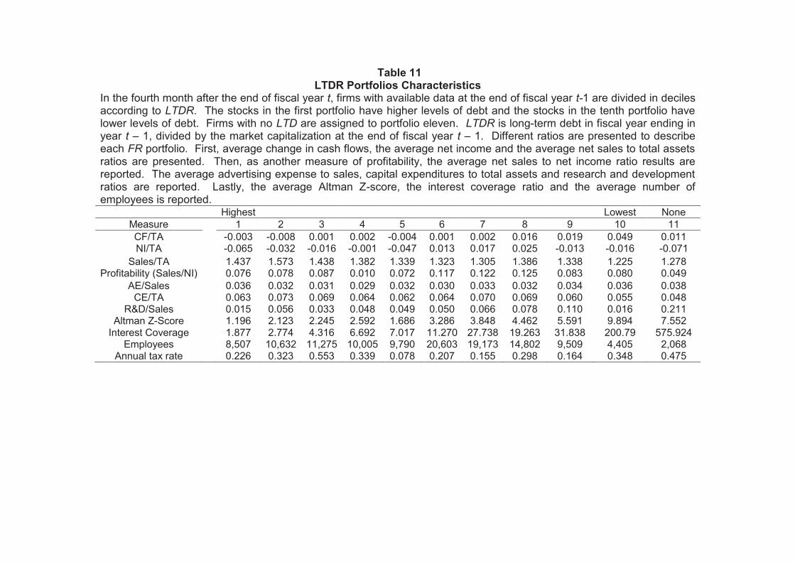
Table 11 LTDR Portfolios Characteristics

In the fourth month after the end of fiscal year t, firms with available data at the end of fiscal year t-1 are divided in deciles according to LTDR. The stocks in the first portfolio have higher levels of debt and the stocks in the tenth portfolio have lower levels of debt. Firms with no LTD are assigned to portfolio eleven. LTDR is long-term debt in fiscal year ending in year t – 1, divided by the market capitalization at the end of fiscal year t – 1. Different ratios are presented to describe each FR portfolio. First, average change in cash flows, the average net income and the average net sales to total assets ratios are presented. Then, as another measure of profitability, the average net sales to net income ratio results are reported. The average advertising expense to sales, capital expenditures to total assets and research and development ratios are reported. Lastly, the average Altman Z-score, the interest coverage ratio and the average number of employees is reported.

Highest Lowest None Measure 1 2 3 4 5 6 7 8 9 10 11 CF/TA -0.003 -0.008 0.001 0.002 -0.004 0.001 0.002 0.016 0.019 0.049 0.011 NI/TA -0.065 -0.032 -0.016 -0.001 -0.047 0.013 0.017 0.025 -0.013 -0.016 -0.071

Sales/TA 1.437 1.573 1.438 1.382 1.339 1.323 1.305 1.386 1.338 1.225 1.278 Profitability (Sales/NI) 0.076 0.078 0.087 0.010 0.072 0.117 0.122 0.125 0.083 0.080 0.049

AE/Sales 0.036 0.032 0.031 0.029 0.032 0.030 0.033 0.032 0.034 0.036 0.038 CE/TA 0.063 0.073 0.069 0.064 0.062 0.064 0.070 0.069 0.060 0.055 0.048

R&D/Sales 0.015 0.056 0.033 0.048 0.049 0.050 0.066 0.078 0.110 0.016 0.211 Altman Z-Score 1.196 2.123 2.245 2.592 1.686 3.286 3.848 4.462 5.591 9.894 7.552

Interest Coverage 1.877 2.774 4.316 6.692 7.017 11.270 27.738 19.263 31.838 200.79 575.924 Employees 8,507 10,632 11,275 10,005 9,790 20,603 19,173 14,802 9,509 4,405 2,068

Annual tax rate 0.226 0.323 0.553 0.339 0.078 0.207 0.155 0.298 0.164 0.348 0.475

Portfolio Characteristics

To describe the firms in each portfolio different characteristics are presented. Table

10 reveals that the most underfunded and the overfunded firms are smaller and tend to

be value firms. The most underfunded firms portray poor financial and operating

performance; spend a smaller amount on advertising, research and development and

operating assets; and have a higher probability of bankruptcy. The most underfunded

firms appear to be overpriced and the overfunded firms appear to be underpriced.

Apparently size may have a role on the way market value firms. Smaller firms tend to

be less exposed and scrutinized by analysts. Quality and quantity of information

available from these firms may have an impact in the way the market evaluates them.

Similarities are observed between FR and LTDR portfolios. Table 11 presents

LTDR portfolio characteristics. As the most underfunded and the overfunded portfolios,

the most levered and the unlevered portfolios have on average the smallest firms of the

set of LTDR portfolios. These are also the most overpriced (levered) and underpriced

(unlevered) firms for these set of portfolios. In contrast to the FR portfolios, the LTDR

portfolios one and ten portray similarities as to a poor financial and operating

performance and spending behavior. In sum, smaller firms may have less access to

different sources of financing (for example bond markets). Analysts do not follow

smaller firms as closer as they do with bigger firms. This may happen because of less

availability of information and less news exposure. Because of their lessen ability to

raise funds, smaller firms may be more inclined to underfund their pension plans.

Higher underfunding levels may be accompanied by high levels of LTD in order to

finance the operations and the pension plans.

VI. Conclusions

This study investigates if investors efficiently incorporate DB pension plan

information in stock prices. Fama and French three factor (1993) and four factor

models results reveal that the market inefficiently incorporates DB pension plan

information. The results are consistent with other studies (Franzoni and Marín 2006,

Godwin and Key 1998).

The results suggest that investors are not paying enough attention to the

implications of the current underfunding for future earnings and cash flows.

Furthermore, portfolio characteristics suggest that the most underfunded and the

overfunded firms are smaller and tend to be value firms. The most underfunded firms

face poor financial and operating performance; tend to spend less on advertising,

research and development and operating assets; and have a higher probability of

bankruptcy. These characteristics make them comparable to value firms. The most

underfunded firms appear to be overpriced and the overfunded firms appear to be

underpriced. Apparently, size has an important role in the way firms are evaluated by

investors. These findings may suggest that smaller firms face limitations to access

different sources of external funds or have exhausted the available sources.

Asymmetries of information may have an indirect relation to size. Because of these

limitations smaller firms may possibly use underfunding as another source of funds.

In contrast with previous research, investors’ reactions to DB pension plan

information were compared to reactions to long-term debt ratios. The results reveal that

the market is also inefficient incorporating long-term debt information. Similar to the

findings of FR portfolios, the most levered and the unlevered portfolios have on average

the smallest firms of the set of LTDR portfolios. Firms in these portfolios are the most

overpriced (levered) and underpriced (unlevered) firms. They also portray a poor

financial and operating performance and higher bankruptcy risk. Smaller firms may

have less access to different sources of financing. As a consequence of information

asymmetries, these firms may face more difficulties to raise funds. And, as the sources

of funds diminish, firms may be more inclined to underfund their pension plans.

In order to verify if the market is inefficient incorporating pension plan and long-term

debt information, this study integrates hedge portfolio tests. Tests’ results corroborate

that the market overprices firms that have severely negative funding status. Investment

strategies short in the most underfunded firms and long in the least underfunded or

overfunded firms yield positive returns for at least three years after portfolio formation.

These tests also reveal similarities between market valuations of underfundings in DB

pension plans and long-term debt information. Investment strategies short in highly

levered firms and long in the least or over levered firms yield positive returns. The

identified inefficiencies may result from market’s inability to integrate information and to

identify future consequences related to long-term commitments. Other studies may

offer some explanations to these results. Investors may be focusing in the optimal

leverage range for firms (Brigham and Gapenski 1985), debt ratings (Carroll and

Niehaus 1998), or they are just “fixating” on earnings figures (Sloan 1996).

References

Banz, R.W., and Breen, W. J., (1986). Sample-Dependent Results Using Accounting and Market Data:

Some Evidence. The Journal of Finance, 41, 4, 779-793. Becheey, M., Gruen, D. and Vickery, J. (2000). The Efficient Market Hypothesis: A Survey. Research

Discussion Paper Reserve Bank of Australia 2000-01. Boyd, J., and Prescott, E., (1986). Financial Intermediary Coalitions. Journal of Financial Theory 38,

211-232. Brigham, E.F. and Gapenski, L.C. (1985). Financial Management: Practice and Theory, 4

th Edition, 1977.

Carroll, T. J., and Niehaus, G., (1998). Pension Plan Funding and Corporate Debt Ratings. The Journal

of Risk and Insurance, 65, 3, 427-441. Chan, L. K. C., Jegadeesh, N., and Lakonishok, J., (1996). Momentum Strategies. The Journal of

Finance, 51, 5, 1681-1713. Diamond, D. W., (1984). Financial Intermediation and Delegated Monitoring. Review of Financial

Studies 51, 393-414. Fama, E., (1985). What's Different About Banks? Journal of Monetary Economics 15, 29-39. Fama, E., L. Fisher, M.C. Jensen, and R.W. Roll (1969). The Adjustment of Stock Prices to New

Information. International Economic Review, 10, 1-27. Fama, E. F., and French, K. R., (1993). Common Risk Factors in the Returns on Stocks and Bonds. The

Journal of Financial Economics, 33, 1, 3-56. Foster III, T. W., Randall, J. D., Vickery, D. W., (1986). The Incremental Information Content of the Annual

Report. Accounting and Business Research, 16, 62, 91-98. Franzoni, F. A., and Marín, J. M., (2006). Pension Plan Funding and Stock Market Efficiency. The

Journal of Finance, 61, 2, 921-956. Godwin, N. H., and Key, K. G., (1998). Market Reaction to Firm Inclusion on the Pension Benefit Guaranty Corporation Underfunding List (March). Retrieved October 24, 2007, from SSRN Web Site: http://ssrn.com/sol3/papers.cfm?abstract_id=115500 Jegadeesh, N., Titman, S., (1993). Returns to Buying Winners and Selling Losers: Implications for Stock

Market Efficiency. The Journal of Finance, 48, 1, 65-91. Jin, L., Merton, R. C., and Bodie, Z., (2006). Do a Firm's Equity Returns Reflect the Risk of its Pension

Plan? The Journal of Financial Economics 81.1, 1-26.

Leland , H. E., and Pyle, D. H., (1977). Informational Asymmetries, Financial Structure, and Financial

Intermediation. The Journal of Finance 32, 371-387. Livnat, J., (1984). Disclosure of Pension Liabilities: The Information Content of Unfunded Vested Benefits

and Unfunded Past Service Cost. Journal of Business, Finance Accounting, 11, 1, 73-88. Lo, A.W. and MacKinlay, A.C. (1999). A Non-Random Wlak Down Wall Street, Princeton University

Press, Princeton N.J. Lo, A.W., Mamaysky, H and Wang, J. (2000). Computational Algorithms, Statistical Inference, and

Empirical Implementation. The Journal of Finance, 55, 4, 1705-1765. Malkiel, B., (2003). The Efficient Market Hypothesis and Its Critics. Journal of Economic Perspectives,

17, 1, 59-82. Miller, E.M., (1977). Debt and Taxes. The Journal of Finance, 32, 2, 261-275. Miller, M. H., and Rock, K., (1985). Dividend Policy under Asymmetric Information. The Journal of

Finance, 40, 4, 1031-1051. Modigliani, F., Miller, M. H., (1958). The Cost of Capital, Corporation Finance and Theory of Investment.

The American Economic Review, 48, 3, 261-297. Myers, S., (2001). Capital Structure. Journal of Economic Perspectives 15, 2, 81-102. Myers, S., and Majluf, N., (1984). Corporate Financing and Investment Decisions When Firms Have

Information That Investors Do Not Have. Journal of Financial Economics 13, 187-221. Phillips, A. L., and Moody, S. M., (2003). The Relationship Between Pension Plan Funding Levels and

Capital Structure: Further Evidence of a Pecking Order. Journal of the Academy of Business and Economics, January 2003.

Rauh, J., (2006). Investment and Financing Constraints: Evidence From the Funding of Corporate

Pension Plans. The Journal of Finance 61, 33-61.

Ross, S. A., (1977). The Determination of Financial Structure: The Incentive-Signalling Approach. The Bell Journal of Economics, 8, 1, 23-40.

Sloan, R. G., (1996). Do Stock Prices Fully Reflect Information in Accruals and Cash Flows About Future

Earnings? The Accounting Review, 71, 3, 289-315. Stefanescu, Irina, (2005). Capital Structure Decisions and Corporate Pension Plans. Working Paper.

University of South Carolina. Stober, T. L., (1986). The Incremental Information Content of Financial Statement Disclosures: The Case

of LIFO Inventory Liquidations. Journal of Accounting Research, 24, 138-160. Stober, T. L., (1993). The Incremental Information Content of Receivables in Predicting Sales, Earnings,

and Profit Margins. Journal of Accounting, Auditing and Finance, 8, 4, 447-473.

Welch, I., (2004). Capital Structure and Stock Returns. The Journal of Political Economy, 112, 1, 106-131.

Xie, H., (2001). The Mispricing of Abnormal Accruals. The Accounting Review, 76, 3, 357-37.

information content of pension status and long-term...

Documents