Information, Preference Kinks, and the Endowment E¤ect

Robert G. Chambers and Tigran Melkonyan1,2

April 19, 2005

1Department of Agricultural and Resource Economics, University of Maryland, College Park.2First Draft. Please don�t cite.

An artefact of experimental economics is the presence of perceptible, and sometimes quite large, diver-

gences between an individual�s willingness to pay (WTP) for a commodity and his or her willingness to

accept (WTA). Because this phenomenon has been observed for common objects (cups, pens, pencils) that

seemingly convey small, if not imperceptible, income e¤ects, it seems to contradict standard microeconomic

intuition that there exists a single price at which an individual is indi¤erent between being a buyer and

seller of a commodity. It has also been widely noted, and veri�ed experimentally (Shapira and Venezia

(2004)), that behavior in insurance markets contradicts expected-utility theory�s prediction that risk-averse

individuals should prefer insurance with deductibles to either no-deductible full insurance or insurance with

very small deductibles (Mossin (1969)).

These apparent anomalies have received theoretical explanations that hinge, in a fundamental sense, on

nonsmooth preference structures. For example, prospect theory explains no-trade results by the presence

of an �endowment e¤ect�that can be identi�ed with a kink in the individual�s preference map (Kahneman

and Tversky (1979) and Tversky and Kahneman (1992)). Similarly, Dow and Werlang (1992) have shown

for Choquet Expected Utility (CEU) preferences that price intervals can exist over which an individual will

refuse either to buy or sell small amounts of a stochastic asset. This observation also rationalizes risk-averse

individuals fully insuring at actuarially unfair odds. Segal and Spivak (1990) o¤er an intuitively similar

explanation of such behavior in terms of ��rst-order�and �second-order�risk aversion.

Mainly in reaction to the experimental evidence, some have conjectured that such �kinky� behavior

might arise from individuals (e.g., student subjects) who are inexperienced in making market transactions

(e.g., Coursey, Hovis, and Schulze (1987); Brookshire and Coursey (1987)). If true, then one might expect

that �endowment�or �no-trade�e¤ects might be eliminated or smoothed as individuals gain experience in

making these transactions. List (2003) has presented �eld experimental evidence that suggests that increased

experience within a given market is associated with smaller endowment e¤ects. Working with data drawn

from active sports memorabilia markets, he �nds that the endowment e¤ect is smaller for experienced

market traders (de�ned as dealers) than for nonexperienced market traders (de�ned as nondealers). Shapira

and Venezia (2004) note a similar phenomenon in their experimental investigations of deductible and no-

deductible insurance. List (2004) details �eld experimental evidence that indicates that market experience

accumulated in one market results in sharply narrowed endowment e¤ects in other markets. This suggests

that the smoothing e¤ects of acquiring market experience can be transferred from one setting to another.

This evidence seems both compelling and intuitive. The goal of this paper is to formalize a decision

model to examine it. The key analytic problems, of course, are to characterize conceptually what it means

to be �more experienced�and what it means for an endowment e¤ect to be smoothed or eliminated by such

experience. The de�nition that we o¤er is that �more experienced�means better informed, and that a better

informed individual has information (formally described as a signal) not available to the less informed. We

de�ne smoothing or elimination of the endowment e¤ect as a narrowing of the WTA/WTP di¤erence.

To model the information process, we work in a framework where individual tastes (attitudes towards

1

risk) remain unchanged, but where beliefs about the state of the world can be in�uenced by the receipt of

information. �More experienced�consumers or market participants are better-informed individuals who have

received information about the state of the world that we assume (but do not explicitly model) is obtained

via market participation. This information is then used to re�ne their belief structure.

Intuitively, the empirical results reported by List (2003) would be rationalized if updating beliefs always

leads to a smaller endowment e¤ect. Not surprisingly, this does not always happen. Acquiring information

does not always cause an individual to converge to a single price at which he or she is willing to exchange a

good. In fact, as we show below, for some belief structures, acquiring information always enhances and never

attenuates endowment e¤ects. A particular case in point occurs when the prior beliefs about the state of

the market are unambiguous (characterized by an unique prior), but where beliefs about the market signals

are characterized by multiple priors. Therefore, it seems important (to us at least) to understand better the

conditions under which the type of behavior reported by List (2003) can be rationalized.

The speci�c model that we choose is the maximin expected utility (MEU) model of Gilboa and Schmeidler

(1989) for risk-averse individuals. Individual preferences over income are modeled by a stable concave utility

structure. Because we work in a framework of uncertainty, we study the no-trade (full insurance) result in

the same context as Dow and Werlang, that is, the decision to buy or sell a single risky asset in a simple

portfolio allocation problem. Hence, the endowment e¤ect, if it occurs, will be found in the neighborhood

of the degenerate random variable. Prior beliefs about the possible states of the world are summarized by a

convex subset of the probability simplex de�ned over the state space.

In what follows, we �rst specify the model. Then we brie�y show how marginal willingness to pay

(MWP) and marginal willingness to sell (MWS) can be represented in terms of appropriately normalized

directional derivatives of the preference structure. These results are then brie�y related to the notion of a

width function, which is de�ned as the upper support function for the di¤erence body (de�ned below) of a

closed convex set. It is shown that the width function corresponds exactly to the di¤erence between MWS

and MWP.

Then we consider information updating, which we treat as revision of the belief structure. We suppose

that the MEU decision-maker uses a prior-by-prior Bayes rule to update her beliefs. This rule involves

updating all priors via Bayes law. Our choice of the preference structure and the update rule is in large part

motivated by a number of recent studies that have provided axiomatic foundations for the intertemporal

versions of the multiple-priors model with prior-by-prior Bayesian updating (Epstein and Schneider (2003),

Hanany and Klibano¤ (2004), Pires (2002), Sarin and Wakker (1998), Siniscalchi (2001), Wakai (2003) and

Wang (2003)). We discuss necessary and su¢ cient conditions for the width function (of the updated priors) to

be larger or smaller than the width function for the original priors. We illustrate these results by considering

three particularly tractable belief structures; a belief structure characterized by a singleton prior over the

payo¤ states, but multiple likelihoods over the signals; priors that constitute the core of a simple capacity;

and a belief structure characterized by a singleton prior over the signals but multiple posteriors over the

2

payo¤ states. Among other results, we show that information updating on average (in a sense to be made

precise below) always leads to an increase in the divergence between WTP and WTA. We also show, in our

framework, a result originally due to Levi (1981) and Giron and Rios (1981) that prior-by-prior updating is

equivalent to updating the extreme points of the original set of priors. This observation de�nes an algorithm

that can be used to check for the presence of price smoothing for an arbitrary belief structure. The paper

then concludes.

1 The Model

The state space is �nite and denoted by = ���, where � = f�1; :::; �Ng and � = f�1; :::; �Sg: � denotes

the �-algebra of all events of ; i.e. � = 2: Let f�sg �NSi=1

(�i; �s) ; f�s1 ; :::; �stg �tS

j=1

NSi=1

��i; �sj

�and

f�ig �SSs=1

(�i; �s) : For the reasons that will become apparent shortly, f�ig0s are called signals and f�sg0s

are called payo¤ events. � denotes the set of all additive probability measures over � and p denotes a

generic element of �. �S denotes the S-dimensional probability simplex.

We study a decision-maker who allocates a �xed amount of income I between a riskless asset that pays

1 in all states of nature and a stochastic asset that pays ys for payo¤ event f�sg: The decision-maker can

take either a short (sell) or a long position (buy) in the risky asset. The prices of the safe and stochastic

assets are 1 and q; respectively. Let t 2 < denote the proportion of income I invested in the risky asset. The

decision-maker�s income contingent on the realization of event f�sg is given by

zs = (1� t)I +tI

qys for s = 1; :::; S: (1)

Thus, z is a random variable that assumes the same value zs in the states (�1; �s) ; :::; (�N ; �s) : We denote

by 1 2 <S the degenerate random variable that pays 1 in each payo¤ event.

The decision-maker�s beliefs over � are represented by a convex set P � � of probability distributions

over �: The decision-maker has maximin expected utility (MEU) preferences3 that are represented by

W (u (f(�))) = inf(X�2

p (f�g)u(f(�)) : p 2 P); (2)

where f : ! < is an act (random variable) mapping the state space to the outcome space (which we

take to be the bounded reals); and u is a monotone, concave utility function giving the decision-maker�s

attitudes towards wealth and risk. With no true loss of generality, we assume that u is di¤erentiable in the

neighborhood of 1:

Let P� denote the restriction of P to payo¤ events f�1g; :::; f�Sg: That is, to each p 2 P � � there

corresponds a unique � = (� (f�1g) ; :::; � (f�Sg)) 2 P� � �S with � (f�sg) = p (f�sg) for all s = 1; :::; S:

3The MEU model is axiomatized in an Anscombe-Aumann framework by Gilboa and Schmeidler (1989) and in a Savage

framework by Casadesus-Masanell et al. (2000).

3

Thus; P� is the orthogonal projection of P and, hence, it inherits convexity from P.

For z � [z1; :::; zS ] given by (1), the decision-maker�s objective function is

W (u (z)) = inf

(SXs=1

� (f�sg)u(zs) : � 2 P�); (3)

where u (z) � [u (z1) ; :::; u (zS)].

We close this section with a brief discussion of some subclasses of MEU preferences.

Example 1 To introduce the �rst subclass, some new notation is needed. A capacity is a set function v : �!

[0; 1] such that (i) v(;) = 0; (ii) v() = 1; and (iii) v(A) � v(B) for all A;B � and A � B: An additive ca-

pacity is a probability measure. The capacity, v; is k-monotone if v�

kSi=1

Ai

��

PI�f1;:::;kg

I 6=?

(�1)jIj+1v�Ti2IAi

�for all Ai 2 �; 1 � i � k; where jIj denotes cardinality of the set I: An 1�monotone capacity (k = 1)

is alternatively called a belief function. A 2-monotone capacity is also called supermodular or convex.3 The

core of the capacity v is the closed, convex, and bounded set:

C(v) = fp 2 � : p(A) � v(A);8A 2 �g: (4)

C(v) is by construction a polytope. When v is supermodular, C (v) is non-empty, v is balanced, and v(A) =

min fp(A) : p(�) 2 C(v)g for all A 2 �. When P is the core of some supermodular capacity v; the decision-

maker�s preference functional (3) has Schmeidler�s (1989) Choquet expected utility (CEU) form

W (u (f(�))) =Z

u(f(�))dv =Z 1

0

v (f� : u (f(�)) � tg) dt+Z 0

�1[v (f� : u (f(�)) � tg)� 1] dt; (5)

where the �rst integration is in the sense of Choquet (1953-4). When P = C(v) for some supermodular

capacity v and z1 � z2 � ::: � zS

W (u (z)) =

S�1Xs=1

[u (zs)� u (zs+1)] v (f�1; :::; �sg) + u (zS) : (6)

Example 2 Because the class of CEU preferences with a supermodular capacity coincides with the intersec-

tion of the classes of CEU and MEU preferences and a k�monotone capacity (k 2 [2;1]) is also l�monotone

for all l = 1; :::; k; MEU preferences considered in this paper include as special cases all CEU preferences

with a k�monotone capacity for all k 2 [2;1].

Example 3 Subjective expected utility is the special case where P = fpg ; a singleton set.3Early literature on ambiguity suggests that supermodularity of a capacity represents uncertainty (or ambiguity) aversion.

This interpretation has been recently challenged (see, for example, Epstein (1999) and Ghirardato and Marinacci (2002)).

4

2 Marginal Willingness to Pay and to Sell

The central analytic observation of the paper is based upon simple geometric point. An individual�s marginal

willingness to pay (MWP) for (or marginal willingness to sell (MWS)) an asset equals an appropriately

normalized directional derivative of his or her preference function. Such directional derivatives for convex

preferences are superlinear (positively linearly homogeneous and superadditive). Therefore, they can be

recognized as (minimal) support functions for a closed convex set, which corresponds to the superdi¤erential

of the individual�s preferences. Di¤erences between marginal willingness to pay and marginal willingness

to sell, which de�ne the no-trade zone of prices, simply measure the width (in a sense to be made precise

below) or diameter of this superdi¤erential in the direction of the asset involved. If the superdi¤erential has

zero width (it corresponds to a single point of measure zero) in that direction, the no-trade zone of prices

disappears, and individuals behave in accordance with expected utility theory. Receiving information in

the form of a signal can either increase the superdi¤erential�s width or narrow it. If it narrows the width

of the superdi¤erential, the no-trade zone (the endowment e¤ect) narrows and individuals converge to the

predictions from expected utility theory. On the other hand if the superdi¤erential�s width increases, the

endowment e¤ect is enhanced.

W; given by (3), is the (minimal) support function for P�: Thus, it is superlinear (positively linearly

homogeneous and superadditive) in u. By construction, it is also translatable in the direction of the sure

thing, that is

W (u+�1) =W (u) + �; � 2 <:

Hence, by basic results on convex sets and their support functions (Rockafellar, 1970)

P� =�� 2 <S : �0u �W (u) for all u 2 <S

:

For any u 2<S ; the superdi¤erential of W (�) is the closed convex set:

@W (u) =�v 2<S :W (u) + v (u0 � u) �W (u0) for all u0 2 <S

: (7)

The one-sided directional derivative of W (u) in the direction of u� is de�ned:

W 0 (u;u�) = lim�!0+

W (u+�u�)�W (u)

�:

W 0 is superlinear in u; and by basic results on proper concave functions (Rockafellar, 1970), it is the support

functional for @W (u) :

W 0 (u;u�) = inf f�0u�: � 2 @W (u)g ; (8)

whence

@W (u) = f� : �0u� �W 0 (u;u�) for all u�g : (9)

5

From (7) and translatability for z = �1; � 2 <

@W (u (�)1) = f� : �0 (u� u (�)1) �W (u)�W (u (�)1) for all ug

= f� : �0 (u� u (�)1) �W (u)� u (�) for all ug

= f� : �0 (u� u (�)1) �W (u� u (�)1) for all u� u (�)1g

= P�: (10)

Carlier and Dana (2003), Ghirardato et al. (2004) and Chambers and Melkonyan (2005) obtain a similar

result.

From an initial position of ze; the gain associated with acquiring asset y 2 <S is

W (u (ze+y))�W (u (ze)) :

For marginal movements in the direction of y and u di¤erentiable, this gain is measured by the directional

derivative

W 0 (u (ze) ;u0 (ze) � y) ;

where u0 (ze) = (u0 (ze1) ; ::; u0 (zeS)) and, form;n 2 <S ;m � n denotes the component-wise product of the two

vectors, (m1n1; :::;mSnS) : Therefore, starting from an initial position of z = 1; which in the asset allocation

problem corresponds to an initial position of t = 0 where no funds are invested in the risky asset, the MWP

for y measured in units of the riskless asset, 1; is

W 0 (u (1)1;u0 (1)y)

W 0 (u (1)1;u0 (1)1)=

W 0 (u (1)1;y)u0 (1)

W 0 (u (1)1;1)u0 (1)=W 0 (u (1)1;y)

W 0 (u (1)1;1)=W 0 (u (1)1;y) (11)

= inf

(SXs=1

� (f�sg) ys : � 2 P�)� eP� (y) :

In the absence of income e¤ects and for small enough changes, WTP corresponds to MWP. The superlinearity

of W 0 in y manifests the fact that the MWP is determined by multiplying the asset by a nonlinear decision

weight, which is chosen conservatively. Accordingly, MWP has the natural interpretation as the most

conservative (over the set P�) evaluation of the asset�s expected value. By similar reasoning, the MWS is

the most optimistic evaluation of the asset�s expected value,

�W 0 (u (1)1;�y) = sup(

SXs=1

� (f�sg) ys : � 2 P�)� eP� (y) :

The literature on imprecise probabilities (Walley, 1991) refers to MWP and the MWS as the the lower and

upper previsions, respectively, of the random variable y: We, therefore, conclude:

Lemma 4 An individual with preferences given by (3) will not trade the risky asset y in the neighborhood

of the sure thing if and only if

q 2 (eP� (y) ; eP� (y)) : (12)

6

Because our interest is in determining circumstances under which endowment e¤ects either decrease or

increase, Lemma 4 is of particular importance. It shows that attention can be restricted to the upper and

lower support functions for P�. It is of particular interest to consider the MWP and the MWS for lotteries

de�ned over the payo¤ events f�sg ; s = 1; 2; :::; S: Denoting each such lottery by rs; we have from the above

W 0 (u (1)1; rs) = inf�� (f�sg) : � 2 P�

� � (f�sg) ;

and

�W 0 (u (1)1;�rs) = sup�� (f�sg) : � 2 P�

� �� (f�sg) :

� (f�sg) and �� (f�sg) are frequently referred to as the lower and upper probabilities, respectively, for the

payo¤ event f�sg over the credal set P� (Smith (1961), Good (1962), Dempster (1966, 1967, 1968), Levi

(1980), Wolfenson and Fine (1982), Walley (1991)). It follows trivially that an individual will refuse to either

buy or sell a lottery ticket for rs if the price falls in between the upper and lower probabilities.

Dow and Werlang (1992) derive an analog to Lemma 4 for a subclass of supermodular CEU preferences.

Lemma 4 extends their result to the entire class of MEU preferences with a convex set of priors. The interval,

(eP� (y) ; eP� (y)) ; which is often called the no-trade price zone, and the interval, (� (f�sg) ; �� (f�sg)) ; which

is often called the probability interval, have a geometrically appealing interpretation to which we now turn.

2.1 Width

For an arbitrary convex set K � <S ; its Minkowski width (alternatively called width or breadth function) in

the direction y 2 <S is the di¤erence between its upper and lower supporting hyperplanes in the direction

y (Bonnessen and Fenchel (1948); Schneider (1993); Averkov (2004)).1 Mathematically, the width function

for K, !K : <S ! <; is de�ned:

!K (y) = sup f�0y : � 2 Kg � inf f�0y : � 2 Kg :

Because it is the di¤erence between an upper and lower support function, !K (y) is sublinear in y. By

construction, it is also translation invariant:

!K+k (y) = !K (y) ; k 2 <S : (13)

By translation invariance and sublinearity, !K is the (upper) support function for the closed, convex set

(Schneider, 1995)

DK =�� 2 <S : !K (y) � �0y for all y 2 <S

(14)

= K �K = fx : x = k� k0;k 2 K;k0 2 Kg1By usual convention, y is taken to be of unit length in the de�nition of the width function. In what follows, we ignore the

obvious normalization.

7

which is referred to as the di¤erence body of K: DK is convex and centered at the origin. Hence, f0g 2 DK

for all K and when K is a singleton set, DK = f0g ; and !K (y) = 0 in all directions.

In the neighborhood of the sure thing, the length of the MWS/MWP interval (the no-trade price zone)

is exactly measured by the support function for DP�

!P� (y) = eP� (y)� eP� (y) = sup��y : � 2 DP�

:

Hence, MWP and MWS always coincide if and only if P� is a singleton set. Dow and Werlang (1992) de�ne

the Minkowski width of P� in the direction of the lotteries:

!P� (rs) = �� (f�sg)� � (f�sg) ;

as the uncertainty aversion associated with payo¤ event f�sg : Their Lemma 3.2 follows trivially from the

requirement that !P� (rs) = 0 for all events. De�nitions of uncertainty aversion vary considerably across

di¤erent authors (Schmeidler, 1989; Epstein, 1999; Ghirardato and Marinacci, 2002; Grant and Quiggin,

2005). No one de�nition seems to have been uniformly adopted. Therefore, in what follows we shall call

!P� (rs) the SDW uncertainty aversion associated with payo¤ event f�sg :

3 Belief Revision

We envision that market participation costlessly conveys information to individuals that non participants

do not possess. That information is in the form of signal about the ultimate state of Nature. Because we

do not explicitly model what constitutes a �signal� event, other than that it is a subset of ; there is no

presumption that the signal is speci�c to the market modelled by our payo¤ events. Hence, the information

can be speci�c about that market, but it need not be.

Formally, this signal will correspond to observing an event of the form, f�ig (i = 1; :::; N). Thus, the

information structure is given by the �ltration (Ft)2t=0 with F0 = f?;g ; F1 = f��algebra generated by

events f�1g ; f�2g ; :::; f�Ngg; and F2 = �: The more experienced decisionmaker uses this signal to update his

or her original set of priors using a prior-by-prior Bayes rule. Thus, for f�ig with inf fp(f�ig) : p(�) 2 Pg > 0,

the conditional probability measure given f�ig is de�ned by Bayes rule for every p 2 P by

p(Ajf�ig) =p(A \ f�ig)p (f�ig)

; 8A 2 �:

The set of posterior probabilities updated by the prior-by-prior Bayesian rule is

P( f�ig) = fp(�jf�ig) : p 2 Pg :

Levi (1980) and Kyburg (1987) demonstrate that P( f�ig) is a convex set.

P�( f�ig) denotes the restriction of P( f�ig) to states (�i; �1) ; :::; (�i; �S) and � (�jf�ig) denotes a generic

element of P�( f�ig): P( f�ig) and P�( f�ig) can be put in a one-to-one correspondence. P�( f�ig) is the

8

orthogonal projection of P( f�ig) while P( f�ig) can be reconstructed from P�( f�ig) by using additivity of

probability measures. P�( f�ig) inherits convexity from P( f�ig):

Let m (f�ig) denote the probability of signal f�ig : Obviously, m (f�ig) = p (f�ig) for p 2 P. Denote

the set of probabilities over signals by

M =

�m (�) : 9p 2 P such that m (f�ig) =

SPs=1

p(f�i; �sg) for all i 2 f1; :::; Ng�:

Epstein and Schneider (2003) demonstrate that, when conditional preferences satisfy axioms of the (static)

MEU model, dynamic consistency in the sense of Machina (1989)2 is equivalent to the rectangularity of the

set of priors and prior-by-prior Bayesian updating.3 In our model, rectangularity requires:

P� =(

NXi=1

m (f�ig)P�(f�ig) : m(�) 2M):

Rectangularity is the generalization of the standard Bayesian decomposition of priors for the payo¤ events

into its posteriors and marginal prior densities for the signals that is required to permit the logic of backward

induction to be applied to the multiple-priors model.

The decision-maker�s preference functional conditional on the receipt of the signal, f�ig; is

inf

(SXs=1

� (f�sgjf�ig)u (zs) : �(�jf�ig) 2 P�(f�ig)):

By previous developments, the no-trade price zone conditional on receiving signal f�ig is�eP�(f�ig) (y) ; eP�(f�ig) (y)

�:

where

eP�(f�ig) (y) � inf

(SXs=1

� (f�sgjf�ig) ys : �(�jf�ig) 2 P�(f�ig));

eP�(f�ig) (y) � sup

(SXs=1

� (f�sgjf�ig) ys : �(�jf�ig) 2 P�(f�ig)):

We have that

!P�(f�ig) (y) = eP�(f�ig) (y)� eP�(f�ig) (y) = sup��y : � 2 DP�(f�ig)

:

Trivially,

Theorem 5 The receipt of signal f�ig decreases the di¤erence between MWP and MWS for y if and only if

!P� (y) � !P�(f�ig) (y) :

2Dynamic consistency in the sense of Machina (1989) is a requirement that conditional preference relation agree with the

unconditional preference relation restricted to a subset of acts that yield the same outcomes on states of nature that were not

realized. Thus, the risks that have been borne a¤ect the decision-maker�s conditional preferences.3For their special framework, Sarin and Wakker (1998) note that rectangularity implies dynamic consistency.

9

When y takes the form of a lottery, Theorem 5 gives necessary and su¢ cient conditions for the SDW

uncertainty aversion associated with that event to decrease. Just as obviously, the theorem provides necessary

and su¢ cient conditions for the SDW uncertainty aversion to increase.

That probability intervals, and hence SDW uncertainty aversion, can expand upon receipt of information

is a well-recognized phenomenon in the imprecise-probabilities literature. Seidenfeld and Wasserman (1993)

de�ne contraction and dilation of probabilities to classify such phenomena. The probability interval for

payo¤ event f�sg dilates if

� (f�sgjf�ig) � � (f�sg) � �� (f�sg) � �� (f�sgjf�ig) ;

and contracts if

� (f�sg) � � (f�sgjf�ig) � �� (f�sgjf�ig) � �� (f�sg) :

Trivially, Theorem 5 provides a necessary but not su¢ cient condition for a contraction of the probabil-

ity interval associated with payo¤ event f�sg: In dealing with a stochastic asset, we will invoke a similar

terminology, saying, for example, that the no-trade price zone dilates conditional on signal f�ig if

eP�(f�ig) (y) � eP� (y) � eP� (y) � eP�(f�ig) (y) :

We also de�ne

De�nition 6 The no-trade price zone for asset y shrinks conditional on signal f�ig if

!P� (y) � !P�(f�ig) (y) :

De�nition 7 The no-trade price zone for asset y expands conditional on signal f�ig if

!P� (y) � !P�(f�ig) (y) :

We use the terminology uniform shrinkage, for example, if shrinkage occurs for all y or all lotteries as

appropriate. The notions of dilation (contraction) and expansion (shrinkage) are closely linked. The latter is

a necessary, but not su¢ cient, condition for the former. If the no-trade price zone shrinks, it obviously cannot

dilate, and if the no-trade price zone expands, it cannot contract. We employ separate terminology because

each is relevant to a di¤erent economic setting. For example, in an experimental setting, an experimentalist

might elicit WTA andWTP without reference to a particular price. Therefore, in that setting, an experienced

subject, when compared to an inexperienced subject, will have a smaller WTA/WTP gap if and only if his

or her no-trade price zone has shrunk in our sense relative to that of the inexperienced subject.

On the other hand, the notions of dilation and contraction are more relevant to situations where the

focus is on determining whether an individual is more or less likely to be willing to act as either a buyer or

a seller for a particular asset at a particular price, for example, q in our notation. For example, if it can

be established that a more experienced individual�s no-trade price zone contracts as a result of the receipt

10

of information, then one might reasonably say that that individual would be less likely to fully ensure at a

given set of market odds than a less informed individual.

Almost trivially,

Theorem 8 The no-trade price zone uniformly shrinks conditional on signal f�ig if and only if DP�(f�ig) �

DP�: The no-trade price zone uniformly expands conditional on signal f�ig if and only if DP� � DP�(f�ig):

It follows immediately from Theorem 8 that if DP� � DP�(f�ig)�DP�(f�ig) � DP�

�the SDW

uncertainty aversion uniformly increases (decreases) conditional on signal f�ig and the no-trade price zone

cannot uniformly contract (dilate) conditional on signal f�ig: Although Theorem 8 is a straightforward

consequence of standard results on convex sets and their support functions, it is especially informative for

certain belief structures. We illustrate by considering three particularly tractable belief structures: a belief

structure characterized by a singleton prior over the payo¤ events, but multiple likelihoods over the signals;

beliefs characterized as the core of a simple capacity; and a belief structure characterized by a singleton prior

over the signal events but multiple posteriors over the payo¤ events.

3.1 Singleton prior over payo¤ events

Suppose the belief structure is characterized by a single prior over the payo¤ events, P� = f�g, but multiple

likelihoods associated with the signals.4 The updating process obviously introduces ambiguity into the

decisionmaker�s belief structure. Accordingly, one expects that no-trade price zones will open up where none

existed before. This is what happens. Trivially, DP� = f0g in this case. Because f0g 2 DK for all closed,

convex K;

DP� � DP�(f�ig)

for all f�ig: Therefore,

Corollary 9 If P� = f�g, the no-trade price zone uniformly expands and SDW uncertainty aversion

uniformly increases for all f�ig:

In one sense, Corollary 9 is irrelevant to the central question posed in this paper. In the setting envisioned

in the corollary, inexperienced participants would exhibit no endowment e¤ect. Observing that the arrival

of a signal that �shakes their faith�about their prior world view may cause them to hesitate about making

certain market transactions does not seem surprising intuitively. Indeed, it seems to accord with much casual

empirical evidence that suggests that individuals �hesitate�after �belief-shaking�events. Its relevance to the

present study is that it demonstrates conclusively that information acquisition is not universally associated

with diminished endowment e¤ects. In this setting just the opposite occurs.

There is another interpretation. Corollary 9 is directly pertinent to our discussion if one identi�es the

information situation that experimental subjects encounter when entering a laboratory setting as receiving a

4Epstein and Schneider (2005) contain a discussion of this situation in terms of Ellsberg�s urn problem.

11

signal that may be ambiguous in nature. Even if they were not predisposed by their prior beliefs to exhibit an

endowment e¤ect, encountering a new situation with which they are unfamiliar might lead them to exhibit

such e¤ects. It is easy to be facile in the manipulation of stylized models to �t apparent empirical facts,

so one must be careful not to push this line of argument too far. However, it does seem to suggest that no

complete empirical validation of the endowment e¤ect perceived in an experimental laboratory setting can be

taken seriously until one formally models and explains the psychological e¤ects of subjecting individuals to

economic experiments. These observations seem to be supported by the results in Plott and Zeiler (2005) who

�nd no signi�cant endowment e¤ects when experiments are designed to minimize �subject misconceptions�

as implicitly de�ned by the experimental literature.

3.2 Simple capacity

Another particularly tractable case emerges when P is the core of a simple capacity. A capacity, v; is simple

if

v(A) =

8<: (1� ")�(A) for all A �

1 for A = ;

where �(�) 2 � and " 2 [0; 1]: Ellsberg (1961) calls (1 � ") the �degree of con�dence�and argues that it

represents the degree of ambiguity. A simple capacity is supermodular (Eichberger and Kelsey (1999)), and

its core is given by

P =C (v(�)) = f(1� ")�g+ "�

where � 2 � and 0 � " � 1: P is, thus, the Minkowski sum of a singleton set f(1� ")�g and the probability

simplex � scaled by ": Simple capacities are often referred to as "�contaminated priors. It follows that

P�=f(1� ")��g+ "�S ; (15)

where �� is the restriction of � to the payo¤ events. Note also that the core of a simple capacity does not

in general satisfy Epstein and Schneider�s (2003) rectangularity condition.

Using (13) and (15) gives:

Theorem 10 For the class of priors given by (15)

!P� (y) = !"�S (y)

= "!�S (y)

= " (max fy1; :::; ySg �min fy1; :::; ySg) :

For the class of simple capacities, the length of the no-trade price interval is " times the maximal possible

evaluation of the asset and its minimal possible valuation by the decision-maker. This manifests two economic

facts. For a simple capacity, the salient probability, ��; is a singleton. That salient probability would yield

a no-trade price interval of zero length if the degree of con�dence were one. In a sense, the salient probability

12

represents the unambiguous component of the decision-maker�s beliefs. On the other hand, if �S represented

the decision-maker�s prior beliefs, one could think of the situation (in terms of payo¤ events) as being totally

ambiguous. Because the simple capacity is a convex combination of a totally unambiguous belief structure

with a totally ambiguous one, there is always some ambiguity. Only the ambiguous component of beliefs

a¤ects the length of the no-trade price interval. The salient probability is only relevant to �xing the position

of the no-trade price interval. For the special case of lotteries it follows trivially that:

Corollary 11 For the class of priors given by (15)

!P� (rs) = "; s = 1; :::; S:

Simple capacities are also particularly convenient because one can obtain the posterior probability sets,

P(f�ig); by updating the capacity itself and then taking the core of the updated capacity. This leads to

extremely sharp results:

Theorem 12 For the class of priors given by (15)

P�(f�ig)=f(1� b")b��g+ b"�S ;where b" = "

"+(1�")�(f�ig) andb��(f�sg) = �(f�ig\f�sg)

�(f�ig) = �(f(�i;�s)g)�(f�ig) . Thus,

!P�(f�ig) (y) = !b"�S (y)

= "̂! (y)

= "̂ (max fy1; :::; ySg �min fy1; :::; ySg) :

Proof. (See Appendix)

It follows immediately from Theorems 10 and 12 that

Theorem 13 For the class of priors given by (15), if 0 < " < 1; the no-trade prize zone uniformly expands

and the SDW uncertainty aversion for payo¤ events uniformly increases conditional on any signal f�ig for

i = 1; :::; N: If " = 0 (no uncertainty) or " = 1 (complete uncertainty); the no-trade price zone and the the

SDW uncertainty aversion for payo¤ events are unchanged conditional on any signal f�ig for i = 1; :::; N:

Thus, the receipt of information never leads to a shrinkage of the no-trade price zone when P is given

by the core of a simple capacity. Endowment e¤ects are magni�ed rather than attenuated. Intuitively, this

implies that the receipt of information will always lead to less trade in the risky asset. This may seem

paradoxical, but it is easily explained. As Eichberger and Kelsey (1999) have shown, receiving a signal

always leads the decision-maker whose beliefs are characterized by a simple capacity to place more weight on

the ambiguous component of his or her belief structure. And because the di¤erence between his or her MWP

and MWS is independent of the salient prior, it follows immediately that the no-trade zone must widen.

13

It follows directly from Theorem 13 that for the class of priors given by (15), if 0 < " < 1; the no-trade

prize zone does not uniformly contract conditional on any signal f�ig for i = 1; :::; N: Herron et al. (1997)

prove a special case of this result in their Proposition 4. Another corollary also follows immediately:

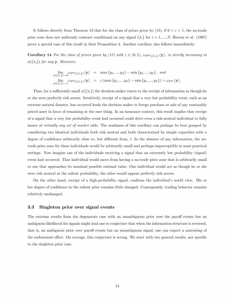
Corollary 14 For the class of priors given by (15) with " 2 (0; 1), !P�(f�ig) (y) ; is strictly increasing in

�(f�ig) for any y: Moreover,

lim�(f�ig)!0

!P�(f�ig) (y) = max fy1; :::; ySg �min fy1; :::; ySg ; and

lim�(f�ig)!1

!P�(f�ig) (y) = " (max fy1; :::; ySg �min fy1; :::; ySg) = !P� (y) :

Thus, for a su¢ ciently small �(f�ig) the decision-maker reacts to the receipt of information as though he

or she were perfectly risk averse. Intuitively, receipt of a signal that a very low probability event, such as an

extreme natural disaster, has occurred leads the decision maker to forego purchase or sale of any reasonably

priced asset in favor of remaining at the sure thing. In an insurance context, this result implies that receipt

of a signal that a very low probability event had occurred could drive even a risk-neutral individual to fully

insure at virtually any set of market odds. The starkness of this corollary can perhaps be best grasped by

considering two identical individuals both risk neutral and both characterized by simple capacities with a

degree of con�dence arbitrarily close to, but di¤erent from, 1: In the absence of any information, the no-

trade price zone for these individuals would be arbitrarily small and perhaps imperceptible in most practical

settings. Now imagine one of the individuals receiving a signal that an extremely low probability (signal)

event had occurred. That individual would move from having a no-trade price zone that is arbitrarily small

to one that approaches its maximal possible rational value. One individual would act as though he or she

were risk neutral at the salient probability, the other would appear perfectly risk averse.

On the other hand, receipt of a high-probability signal, con�rms the individual�s world view. His or

her degree of con�dence in the salient prior remains little changed. Consequently, trading behavior remains

relatively unchanged.

3.3 Singleton prior over signal events

The extreme results from the degenerate case with an unambiguous prior over the payo¤ events but an

ambiguous likelihood for signals might lead one to conjecture that when the information structure is reversed,

that is, an ambiguous prior over payo¤ events but an unambiguous signal, one can expect a narrowing of

the endowment e¤ect. On average, this conjecture is wrong. We start with two general results, not speci�c

to the singleton prior case.

14

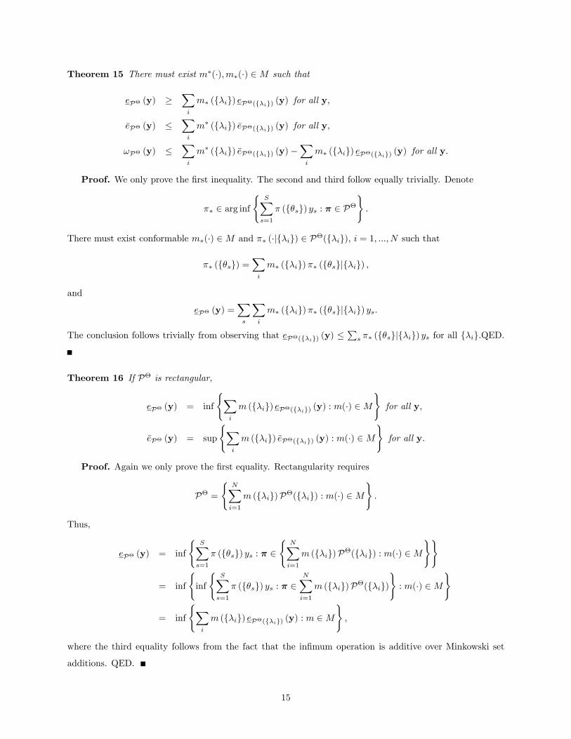
Theorem 15 There must exist m�(�);m�(�) 2M such that

eP� (y) �Xi

m� (f�ig) eP�(f�ig) (y) for all y;

�eP� (y) �Xi

m� (f�ig) �eP�(f�ig) (y) for all y;

!P� (y) �Xi

m� (f�ig) �eP�(f�ig) (y)�Xi

m� (f�ig) eP�(f�ig) (y) for all y:

Proof. We only prove the �rst inequality. The second and third follow equally trivially. Denote

�� 2 arg inf(

SXs=1

� (f�sg) ys : � 2 P�):

There must exist conformable m�(�) 2M and �� (�jf�ig) 2 P�(f�ig); i = 1; :::; N such that

�� (f�sg) =Xi

m� (f�ig)�� (f�sgjf�ig) ;

and

eP� (y) =Xs

Xi

m� (f�ig)�� (f�sgjf�ig) ys:

The conclusion follows trivially from observing that eP�(f�ig) (y) �P

s �� (f�sgjf�ig) ys for all f�ig:QED.

Theorem 16 If P� is rectangular,

eP� (y) = inf

(Xi

m (f�ig) eP�(f�ig) (y) : m(�) 2M)for all y;

�eP� (y) = sup

(Xi

m (f�ig) �eP�(f�ig) (y) : m(�) 2M)for all y:

Proof. Again we only prove the �rst equality. Rectangularity requires

P� =(

NXi=1

m (f�ig)P�(f�ig) : m(�) 2M):

Thus,

eP� (y) = inf

(SXs=1

� (f�sg) ys : � 2(

NXi=1

m (f�ig)P�(f�ig) : m(�) 2M))

= inf

(inf

(SXs=1

� (f�sg) ys : � 2NXi=1

m (f�ig)P�(f�ig)): m(�) 2M

)

= inf

(Xi

m (f�ig) eP�(f�ig) (y) : m 2M);

where the third equality follows from the fact that the in�mum operation is additive over Minkowski set

additions. QED.

15

Theorem 15 implies that �on average� information updating causes no-trade price zones to dilate and

SDW uncertainty aversion to increase. The essence of no-trade price zones is conservatism. In establishing a

MWP for the asset, the decisionmaker accords it his or her lowest possible expected value given their belief

structure. Conversely, in establishing a MWS, the same decisionmaker demands in return his or her highest

possible expected value for the asset. As we discuss further below, this observation is generic to rational

individual behavior and generalizes well past the MEU model to any welfare functional that is Lipschitzian.

Thus, when faced with a set of priors for the payo¤ events, the decisionmaker chooses the most conservative

priors to evaluate his or her purchase decision. In doing so, he or she implicitly �nds a lower and upper

support function. The priors that he or she picks, to be conformable, are appropriate averages drawn from

his or her posterior probability sets. Thus, his or her MWS and MWP can always be viewed as an average

over these posterior sets.

When the individual assesses MWP and MWS after the receipt of information, the action is again

taken conservatively. However, the action is taken conservatively with respect to the set of probabilities

that is relevant for that signal event. �On average�conservative action over individual sets must dominate

conservative action over a single set constructed from the others. Because the individual is not forced to

pick the same underlying posteriors for each signal events, his conservative choices for signal events have to

dominate his conservative choices in the absence of information.

Rectangularity is the condition that is required to permit the logic of backward induction to be applied

in the MEU model. In the standard Bayesian framework, backward induction is essentially justi�ed by the

law of iterated expectations. There, the prior expected value of an asset is the average (taken with respect

to the probability of the signal) of the posterior expectations. In the MEU, the same averaging procedure

cannot be applied because of the multiplicity of priors. Theorem 16 shows, however, that it does apply in

a conservative sense. The prior MWP for an asset is the most conservative average of the posterior MWPs,

and the MWS is the most conservative average of the posterior MWS. Put another way, the prior MWP

(MWS) for the asset is dynamically consistent with its posterior MWPs (MWSs).

The implications of these general results for our analysis are perhaps most clearly seen in the following

corollaries:

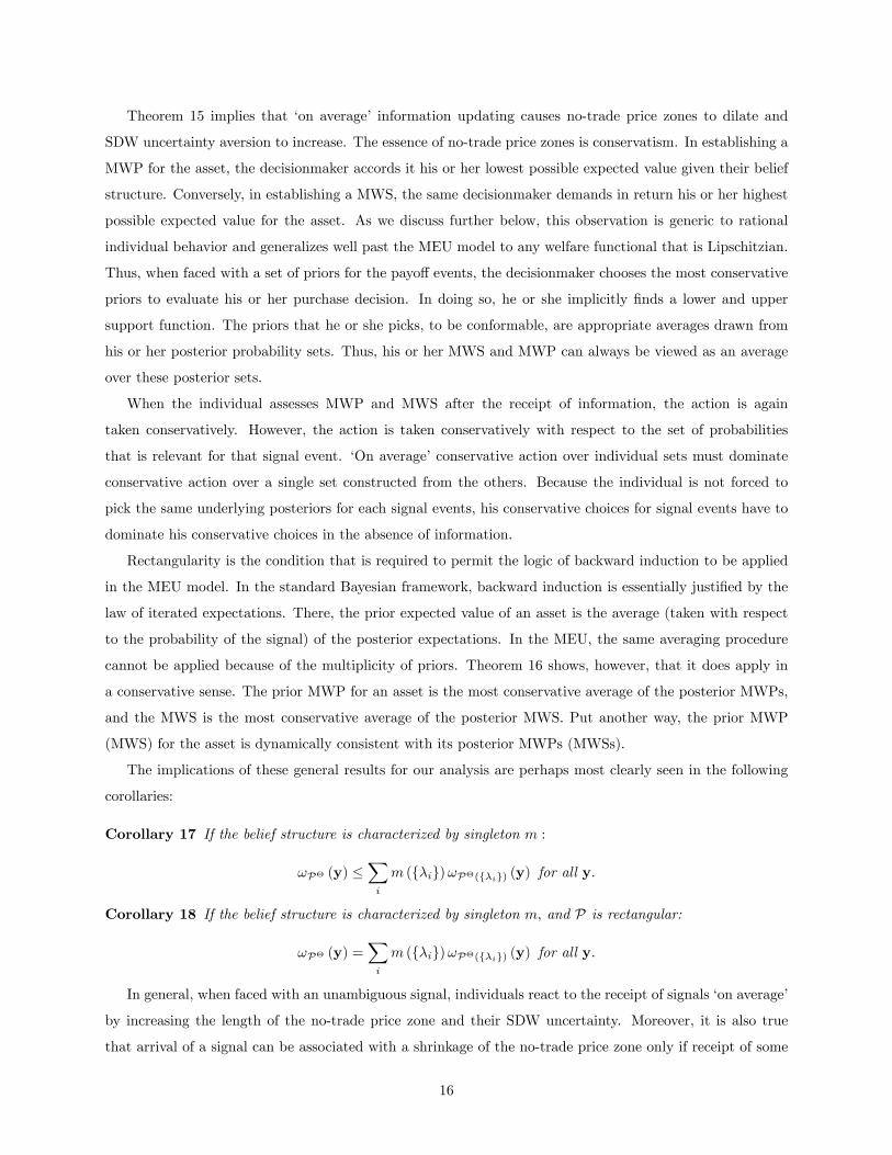
Corollary 17 If the belief structure is characterized by singleton m :

!P� (y) �Xi

m (f�ig)!P�(f�ig) (y) for all y:

Corollary 18 If the belief structure is characterized by singleton m; and P is rectangular:

!P� (y) =Xi

m (f�ig)!P�(f�ig) (y) for all y:

In general, when faced with an unambiguous signal, individuals react to the receipt of signals �on average�

by increasing the length of the no-trade price zone and their SDW uncertainty. Moreover, it is also true

that arrival of a signal can be associated with a shrinkage of the no-trade price zone only if receipt of some

16

other signal is associated with an expansion of a no-trade price zone. Again, this re�ects the conservatism

that is inherent in any divergence between MWS and MWP. Rational individuals hesitate to trade if they

are uncertain that they are trading at correct prices.

In the context of the results presented by List (2003, 2004), one might conclude from Corollary 9 that

the signal received by his �dealers�was of the former type. In a sense that we have not precisely modeled,

it is communicated to them that the state of the world was less ambiguous than the belief structure of the

�nondealers�would suggest. Because �dealers�are obvious repeat participants in markets, this seems quite

intuitive. They have consistently received information that indicates to them in a subjective sense that the

market does obey familiar notions of probability.

Rectangularity models �more rational�behavior in the sense that it is consistent with the requirements

of dynamic consistency. That does not mean that individuals will always be more willing to trade on the

basis of the receipt of an unambiguous signal than in its absence. But it does require that if the endowment

e¤ect is exacerbated by one signal, it must be attenuated by at least one other signal. All news cannot be

bad news in the sense that it stulti�es trading behavior. Some news can cause individuals to pause even

more than they had originally, but there have to exist news events that would have led them to trade more

because their SDW uncertainty aversion has decreased.

4 Algorithms to Verify Uniform Shrinkage and Contraction

The results of the last section suggest that, in many instances, determining whether the endowment e¤ect is

either exacerbated or attenuated as a result of market experience will require the explicit evaluation of both

DP� and DP�( f�ig): Therefore, we now consider algorithms to verify conditions under which no-trade

price zones shrink or expand.

By Minkowski�s Theorem, convex sets can be characterized in terms of their extreme points. Such a

characterization is especially attractive because to obtain a set of posterior probability measures using prior-

by-prior updating one only need to apply Bayes�rule to the extreme points of the set of priors and then take

the resulting convex hull of the updated priors (Giron and Rios (1980) and Levi (1980)).5

Theorem 19 Suppose P is a convex set of priors. Then

DP� = conv

8>>><>>>:z 2 <S : z = (z0 � z00) ; z0; z00 2 �S such that

[z0(f�i; �sg) = p0(f�i; �sg) for all s 2 f1; :::; Sg] and

[z00(f�i; �sg) = p00(f�i; �sg) for all s 2 f1; :::; Sg] for some p0;p00 2 ext(P)

9>>>=>>>; (16)

5Ja¤ray (1992) contains a proof of the result for belief functions.

17

and

DP�( f�ig) = conv

8>>><>>>:z 2 <S : z = (z0 � z00) ; z0; z00 2 �S such thath

z0(f�i; �sg) = p0(f�i; �sg jf�ig) = p0(f�i;�sg)p0(f�ig) for all s 2 f1; :::; Sg

iandh

z00(f�i; �sg) = p00(f�i; �sg jf�ig) = p00(f�i;�sg)p00(f�ig) for all s 2 f1; :::; Sg

ifor some p0;p00 2 ext(P)

9>>>=>>>; ;(17)

where ext(A) denotes the set of extreme points of set A and conv f�g denotes the convex hull.

Proposition 19 provides an algorithm for verifying conditions under which shrinkage, contraction, dilation,

and expansion occur. For strictly convex sets of priors, this algorithm requires evaluating an in�nity of

conditions. However, in a separate study (Chambers and Melkonyan, 2005), we provide conditions under

which arbitrary convex sets can be approximated to an arbitrary degree of closeness in terms of the Hausdor¤

metric in a �nite number of steps. And when P is a polytope, exact results can be obtained in a �nite number

of steps. We turn to that important special case in the next subsection.

4.1 Polytope P

Polytopes arise quite naturally as candidates for representing the decision-maker�s beliefs (Gilboa and Schmei-

dler (1989), Walley (1991) and Epstein and Schneider (2003)). Because the image of a polytope under any

linear transformation is a polytope (Gr¼unbaum (2003, Theorem 3.1.4)), P� is a polytope if P is. Similarly,

because P�( f�ig) is obtained from P( f�ig) via a linear transformation, P�( f�ig) is also a polytope. Be-

cause P� and P�( f�ig) are polytopes and the Minkowski sum of two polytopes is a polytope (Gr¼unbaum

(2003, Theorem 3.1.4)), both DP� and DP�( f�ig) are polytopes if P is.

Polytope A is a subset of B if and only if every vertex of A belongs to B. Combining these observations

with Theorem 8, we obtain the following theorem

Theorem 20 Let P be a polytope. The no-trade price zone shrinks uniformly if and only if every vertex of

DP�( f�ig) belongs to DP�: The no-trade price zone expands uniformly if and only if every vertex of DP�

belongs to DP�( f�ig):

It follows immediately from Theorem 20 that, when P is a polytope, the no-trade price zone cannot

uniformly dilate if every vertex of DP�( f�ig) belongs to DP�: Similarly, the no-trade price zone cannot

uniformly contract if every vertex of DP� belongs to DP�( f�ig):

The following corollary to Theorem 19 characterizes DP� and DP�( f�ig) when P is a polytope.

Corollary 21 Suppose P is a polytope. Then

DP� = conv

8<: z 2 <S : z = (z0 � z00) ; z0; z00 2 �S such that [z0(f�i; �sg) = p0(f�i; �sg) for all s 2 f1; :::; Sg]

and [z00(f�i; �sg) = p00(f�i; �sg) for all s 2 f1; :::; Sg] for some p0;p00 2 vert(P)

9=;18

and

DP�( f�ig) = conv

8<: z 2 <S : z = (z0 � z00) ; z0; z00 2 �S such thathz0(A) = p0(Ajf�ig) = p0(A\f�ig)

p0(f�ig) for all s 2 f1; :::; Sgi

andhz00(A) = p00(Ajf�ig) = p00(A\f�ig)

p00(f�ig) for all s 2 f1; :::; Sgifor some p0;p00 2 vert(P)

9=; :where vert (A) denotes the vertices of set A.

For the class of MEU preferences where P is a polytope, Theorem 20 and Corollary 21 provide an

algorithm that permits veri�cation in a �nite number of steps whether the no-trade price zone uniformly

shrinks, uniformly expands, or does neither. An analytically important subclass occurs when P is the

core of some supermodular or k-monotone (k 2 [2;1]) capacity v. In such instances, a classic result due

to Shapley (1971) identi�es the vertices of P. This knowledge, when combined with Corollary 21 and

Theorem 20, determines if the no-trade price zone shrinks or expands. Thus, it is trivially possible to

use Shapley�s vertices� results to state necessary and su¢ cient conditions for a particular supermodular

capacity to satisfy the conditions of Theorems 8 and 20. These conditions are straightforward to compute

but notationally cumbersome to present. Their very generality seems to preclude (for us) economically

meaningful interpretations.

5 Concluding Remarks

We initiated this research thinking it would be relatively straightforward to identify conditions under which

market experience, as we describe it, would eliminate endowment e¤ects. It seems, however, that there is good

reason to suspect that in the MEU model information provision typically tends to exacerbate endowment

e¤ects rather than attenuate them.

In retrospect, this seems easy to explain. MEU models, in a sense, were reverse engineered to ac-

commodate Ellsberg�s Paradox. Ellsberg�s Paradox seems to depict conservative behavior on the part of

decisionmakers. The MEU model captures this conservatism by using the least auspicious prior to evaluate

any random variable. Seemingly, this conservatism is inherited from the MEU model through the properties

of its directional derivatives, which characterize MWP and MWS and thus WTP and WTA for small enough

changes.

However, it is relatively easy to see that this conservatism in the evaluation of MWP and MWS is not

speci�c to the MEU model. As noted earlier, it is the essence of a rational refusal to trade. For example,

if one speci�ed preferences over income in the payo¤ events by an evaluation function W (y) ; this same

conservatism would be inherited so long as W were Lipschitzian. Following Clarke (1983), the argument

is as follows: If W is Lipschitzian, then it can be shown to possess generalized versions of the directional

derivatives used in this paper (Ghirardato et al. (2004)). These generalized directional derivatives are

superlinear and thus can be viewed as support functionals for a closed, convex set which can be thought of

as the generalization of the superdi¤erential. MWS and MWP are then, respectively, the upper and lower

19

support function for this generalized superdi¤erential in the direction of the asset exactly as in the present

paper.

6 Appendix

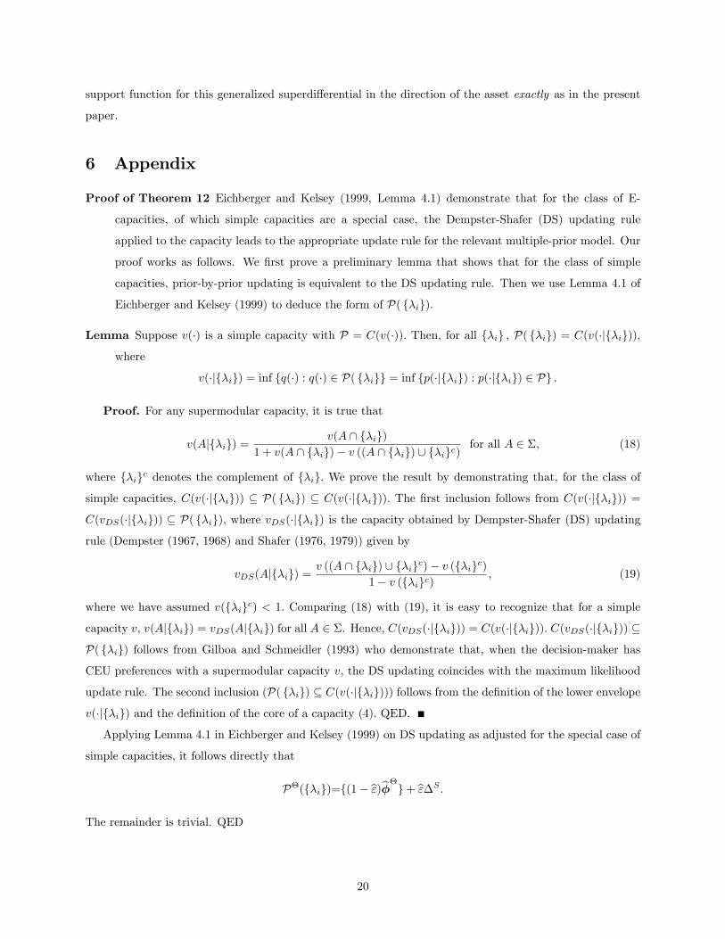
Proof of Theorem 12 Eichberger and Kelsey (1999, Lemma 4.1) demonstrate that for the class of E-

capacities, of which simple capacities are a special case, the Dempster-Shafer (DS) updating rule

applied to the capacity leads to the appropriate update rule for the relevant multiple-prior model. Our

proof works as follows. We �rst prove a preliminary lemma that shows that for the class of simple

capacities, prior-by-prior updating is equivalent to the DS updating rule. Then we use Lemma 4.1 of

Eichberger and Kelsey (1999) to deduce the form of P( f�ig):

Lemma Suppose v(�) is a simple capacity with P = C(v(�)): Then, for all f�ig ; P( f�ig) = C(v(�jf�ig));

where

v(�jf�ig) = inf fq(�) : q(�) 2 P( f�igg = inf fp(�jf�ig) : p(�jf�ig) 2 Pg :

Proof. For any supermodular capacity, it is true that

v(Ajf�ig) =v(A \ f�ig)

1 + v(A \ f�ig)� v ((A \ f�ig) [ f�igc)for all A 2 �; (18)

where f�igc denotes the complement of f�ig: We prove the result by demonstrating that, for the class of

simple capacities, C(v(�jf�ig)) � P( f�ig) � C(v(�jf�ig)): The �rst inclusion follows from C(v(�jf�ig)) =

C(vDS(�jf�ig)) � P( f�ig); where vDS(�jf�ig) is the capacity obtained by Dempster-Shafer (DS) updating

rule (Dempster (1967, 1968) and Shafer (1976, 1979)) given by

vDS(Ajf�ig) =v ((A \ f�ig) [ f�igc)� v (f�igc)

1� v (f�igc); (19)

where we have assumed v(f�igc) < 1: Comparing (18) with (19); it is easy to recognize that for a simple

capacity v, v(Ajf�ig) = vDS(Ajf�ig) for all A 2 �. Hence, C(vDS(�jf�ig)) = C(v(�jf�ig)): C(vDS(�jf�ig)) �

P( f�ig) follows from Gilboa and Schmeidler (1993) who demonstrate that, when the decision-maker has

CEU preferences with a supermodular capacity v, the DS updating coincides with the maximum likelihood

update rule. The second inclusion (P( f�ig) � C(v(�jf�ig))) follows from the de�nition of the lower envelope

v(�jf�ig) and the de�nition of the core of a capacity (4): QED.

Applying Lemma 4.1 in Eichberger and Kelsey (1999) on DS updating as adjusted for the special case of

simple capacities, it follows directly that

P�(f�ig)=f(1� b")b��g+ b"�S :The remainder is trivial. QED

20

Proof for Proposition 19: (16) follows directly from the de�nition of the di¤erence body (14) and the fact

that P� is the restriction of P to events f�1g ; :::; f�Sg :(17) follows from the de�nition of the di¤erence

body (14), the fact that P�(f�ig) is the restriction of P(f�ig) to states f�i; �1g ; :::; f�i; �Sg and the

following Lemma which has been proven by Giron and Rios (1980) and Levi (1980). Because of the

notational di¤erences between Giron and Rios (1980) and Levi (1980) frameworks and ours and the

resulting complexities associated with moving from their notation to ours, we provide a direct proof of

their result in terms of our notation. Note that Ja¤ray (1992) contains a proof of the result for belief

functions. His proof can be easily extended to general convex probability sets.

Lemma 22 (Giron and Rios (1980); Levi (1980)) Suppose P is a convex set of priors. Then P( f�ig) is

the convex hull of the set of points which are the conditionals of the points in ext(P ); i.e.

P( f�ig) = conv�z 2 � : 9p 2 ext(P ) such that z(A) = p(Ajf�ig) =

p(A \ f�ig)p (f�ig)

for all A 2 ��:

Proof. Let

K � conv�z 2 � : 9p 2 ext(P ) such that z(A) = p(Ajf�ig) =

p(A \ f�ig)p (f�ig)

for all A 2 ��:

Our objective is to show that K = P( f�ig). From the de�nition of K; it follows immediately that K �

P( f�ig): To see that the reverse inclusion holds consider an arbitrary element p 2 P. By Carath·eodory�s

Theorem, p can be represented as a convex combination of L extreme points of P; i.e.,

9fpmgLm=1 2 ext(P ) such that p =LP

m=1�mpm; where �m � 0 for all m = 1; ::::; L and

LPm=1

�m = 1:

The conditional of p is given by

p(�jf�ig) =p(�)

p (f�ig)=

LPm=1

�mpm(�)

LPm=1

�mpm(f�ig)=

LPm=1

[�mpm (f�ig) pm(�jf�ig)]

LPm=1

�mpm(f�ig)=

LPj=1

�jpj(�jf�ig) 2 K

where �j =�jpj(f�ig)

LPm=1

�mpm(f�ig)with �j � 0 for all j = 1; ::::; L and

LPj=1

�j = 1: Hence, P( f�ig) � K: Thus,

P( f�ig) = K: QED.

7 References

1. Averkov, G., 2004. Metrical Properties of Convex Bodies in Minkowski spaces. PhD Thesis in Mathe-

matics, Chemnitz University of Technology, Germany.

2. Blackwell, .D., 1951. �Comparison of experiments.� in: J. Neymann (Ed.), Proceedings of the Sec-

ond Berkeley Symposium on Mathematical Statistics and Probability, University of California Press,

Berkeley, pp. 93�102.

21

3. Blackwell, D., 1953. �Equivalent Comparisons of Experiments.�Annals of Mathematical Statistics 24,

pp. 265� 272.

4. Bonnesen, T. and W. Fenchel, 1948. Theory of Convex Bodies. BCS Associates, Moscow, Idaho

[Translation of Theorie der konvexen Körper, Springer, Berlin, 1934 and Chelsea, New York, 1948.

5. Brookshire, D. S. and D. L. Coursey, 1987. �Measuring the Value of a Public Good: An Empirical

Comparison of Elicitation Procedures.�American Economic Review, v. 77, iss. 4, pp. 554-66.

6. Carlier, G. and R. A. Dana, 2003. �Core of Convex Distortions of a Probability.�Journal of Economic

Theory v. 113, iss. 2, pp. 199-222.

7. Casadesus-Masanell, R. Klibano¤, P. and E. Ozdenoren, 2000. �Maxmin Expected Utility over Savage

Acts with a Set of Priors.�Journal of Economic Theory 92, pp. 35�65.

8. Chambers, R. and T.A. Melkonyan, 2005. �Eliciting the Core of a Supermodular Capacity.�Economic

Theory 26 (1), pp. 203-210.

9. Chambers, R. and T.A. Melkonyan, 2005. �Belief Elicitation.�Working Paper.

10. Chateauneuf, A and J.-Y. Ja¤ray, 1989. �Some Characterizations of Lower Probabilities and Other

Monotone Capacities through the Use of M½obius Inversion.�Mathematical Social Sciences 17, pp.

263-283.

11. Chateauneuf, A, Kast, R. and A. Lapied, 2001. �Conditioning Capacities and Choquet Integrals: The

Role of Comonotony.�Theory and Decision 51, pp. 367-386.

12. Choquet, G., �Theory of Capacities.�Ann. Inst. Fourier 5 (1953�4) 131�295.

13. Clarke, F.H., 1983. Optimization and Nonsmooth Analysis. Wiley, New York.

14. Coursey, D.L., Hovis, J.L. and W.D. Schulze, 1987. �The Disparity between Willingness to Accept and

Willingness to Pay Measures of Value.�Quarterly Journal of Economics, v. 102, iss. 3, pp. 679-90.

15. de Finetti, B., 1937. �La prévision: ses lois logiques, ses sources subjectives.�Annales de l�Institute

Henri Poincaré, 7, pp. 1-68.

16. de Finetti, B., 1972. Probability, induction and statistics. The art of guessing. John Wiley & Sons,

London-New York-Sydney, 1972.

17. Dempster, A.P., 1967. �Upper and Lower Probabilities Induced from a Multivalued Mapping.�Annals

of Mathematical Statistics 38, pp. 525�539.

18. Dempster, A.P., 1968. �A Generalization of Bayesian Inference.�Journal of Royal Statistical Society,

Ser. B 30, pp. 205�247.

22

19. Dow, J. and S. Werlang, 1992. �Uncertainty Aversion, Risk Aversion, and the Optimal Choice of

Portfolio.�Econometrica 60, pp. 197-204.

20. Eichberger, J. and D. Kelsey, 1999. �E-Capacities and the Ellsberg Paradox.�Theory and Decision,

v. 46, iss. 2, pp. 107-40.

21. Ellsberg, D., 1961. �Risk, Ambiguity and the Savage Axioms.�Quarterly Journal of Economics 75,

pp. 643-669.

22. Epstein, L.G., 1999. �A De�nition of Uncertainty Aversion.�Review of Economic Studies 66, 579-608.

23. Epstein, L.G. and M. Schneider, 2003. �Recursive Multiple-Priors.�Journal of Economic Theory, v.

113, iss. 1, pp. 1-31.

24. Epstein, L.G. and M. Schneider, 2005. �Learning under Ambiguity.�

25. Fagin, R. and J. Y. Halpern, 1991. �A New Approach to Updating Beliefs.�Uncertainty in Arti�cial

Intelligence 6, pp. 347-374.

26. Gajdos, T., Tallon, J.-M., Vergnaud, J.-C., 2005. Decision Making with Imprecise Probabilistic Infor-

mation. Forthcoming in the Journal of Mathematical Economics.

27. Ghirardato, P. and M. Marinacci, 2002. �Ambiguity Made Precise: A Comparative Foundation.�

Journal of Economic Theory 102, pp. 251-289.

28. Ghirardato, P., F. Maccheroni and M. Marinacci, 2004. �Di¤erentiating Ambiguity and Ambiguity

Attitude.�Journal of Economic Theory, v. 118, iss. 2, pp. 133-73.

29. Gilboa, I., 1987. �Expected Utility Theory with Purely Subjective Non-additive Probabilities.�Journal

of Mathematical Economics 16, pp. 65�88.

30. Gilboa, I. and D. Schmeidler, 1989. �Maxmin Expected Utility with Non-unique Prior.� Journal of

Mathematical Economics 18, pp. 141-153.

31. Gilboa, I. and D. Schmeidler, 1993. �Updating Ambiguous Beliefs.�Journal of Economic Theory 59,

pp. 33�49.

32. Giron, F. J. and S. Rios, 1980. �Quasi-Bayesian behavior: A more realistic approach to decision

making?� in J. M. Bernardo, J. H. DeGroot, D. V. Lindley, and A. F. M. Smith, editors, Bayesian

Statistics, pages 17-38. University Press, Valencia, Spain, 1980.

33. Good, I.J., 1983. Good Thinking: The Foundations of Probability and Its Applications. University of

Minnesota Press, Minneapolis.

23

34. Grant, S, and J. Quiggin, 2005. �Increasing Uncertainty: A De�nition.�Mathematical Social Sciences

49, pp. 117-141.

35. Gr¼unbaum, B., 2003. Convex Polytopes. Springer-Verlag, New York.

36. Hanemann, M.W., 1991. �Willingness To Pay and Willingness To Accept: How Much Can They

Di¤er?�American Economic Review vol. 81 no. 3, pp. 635-647.

37. Hanany, E. and P. Klibano¤, 2004. �Updating Multiple-Prior Preferences.�Working Paper.

38. Herron, T., T. Seidenfeld, L. Wasserman, 1997. �Divisive Conditioning: Further Results on Dilation.�

Philosophy of Science 64, pp. 411�444.

39. Ja¤ray, J.-Y., 1992. �Bayesian Updating and Belief Function.� IEEE Transactions on Systems, Man,

and Cybernetics, Vol. 22, No.5, pp. 1144-1152.

40. Kahneman, D. and A. Tversky, 1979. �Prospect Theory: An Analysis of Decision under Risk.�Econo-

metrica, v. 47, iss. 2, pp. 263-91.

41. Kling, C. L., J. A. List, and J., Zhao, 2003. �The WTP/WTA Disparity: Have We Been Observing

Dynamic Values but Interpreting Them as Static?�Working Paper 03-WP 333, Center for Agricultural

and Rural Development, Iowa State University.

42. Knight, F., 1921. Risk, Uncertainty and Pro�t. New York: Augustus M. Kelley.

43. K½oszegi, B. and M. Rabin, 2005. �A Model of Reference-Dependent Preferences.�Working Paper,

Department of Economics, University of California, Berkeley.

44. Kyburg, H. E., Jr., 1987. �Bayesian and Non-Bayesian Evidential Updating.�Arti�cial Intelligence

31, pp. 271-293.

45. Levi, I. 1980. The Enterprise of Knowledge. MIT Press, Cambridge, Massachusetts.

46. List, J. A., 2003. �Does Market Experience Eliminate Market Anomalies?� Quarterly Journal of

Economics, v. 118, iss. 1, pp. 41-71.

47. List, J. A., 2004. �Neoclassical Theory Versus Prospect Theory: Evidence from the Marketplace.�

Econometrica vol. 72, no. 2, pp. 615-625.

48. Mossin, J., 1969. �Security Pricing and Investment Criteria in Competitive Markets.�American Eco-

nomic Review, v. 59, iss. 5, pp. 749-56.

49. Pires. C. P., 2002. �A Rule For Updating Ambiguous Beliefs.�Theory and Decision 53, Iss. 2, pp.

137-152.

24

50. Plott, C. R. and K. Zeiler, 2005. �The Willingness to Pay/ Willingness to Accept Gap, the �Endowment

E¤ect�and Experimental Procedures for Eliciting Valuations.�forthcoming in the American Economic

Review.

51. Quiggin, J. 1982. �A Theory of Anticipated Utility.�Journal of Economic Behavior and Organization

3, pp. 323-343.

52. Randall, A. and J. R. Stoll, 1980. �Consumer�s Surplus in Commodity Space.�American Economic

Review 71, pp. 449-457.

53. Rockafellar, R.T., 1970. Convex Analysis. Princeton University Press Princeton, N.J.

54. Sarin, R. and P. Wakker, 1998. �Revealed Likelihood and Knightian Uncertainty.� Journal of Risk

and Uncertainty 16, pp. 223�250.

55. Savage, L., 1954. Foundations of Statistics. Wiley, New York.

56. Schmeidler, D., 1989. �Subjective Probability and Expected Utility without Additivity.�Econometrica

57, pp. 571-587.

57. Schneider, R., 1993. Convex Bodies: The Brunn-Minkowski Theory. Cambridge University Press.

58. Segal, U. and A. Spivak, 1990. �First Order versus Second Order Risk Aversion.�Journal of Economic

Theory v. 51, iss. 1, pp. 111-25

59. Seidenfeld, T. and L. Wasserman, 1993. �Dilation for Convex Sets of Probabilities.�Annals of Statistics

21, pp. 1139�1154.

60. Shafer, G., 1976. A Mathematical Theory of Evidence. University of Princeton Press, New Jersey.

61. Shafer, G., 1979. �Allocations of Probability.�Annals of Probability 7, pp. 827�839.

62. Shapira, Z. and I. Venezia, 2004. �An Experimental Study of the Full-Coverage Puzzle.�Working

Paper.

63. Shapley, L.S., 1971. �Cores of convex games.�International Journal of Game Theory, 1, pp. 12-26.

64. Siniscalchi, M., 2001. �Bayesian Updating for General Maxmin Expected Utility Preferences.�Mimeo.

65. Smith, C.A.B., 1961. �Consistency in Statistical Inference and Decision.�Journal of Royal Statistical

Society B 23: 1-25.

66. Sundberg, C. and C. Wagner, 1992. �Generalized Finite Di¤erences and Bayesian Conditioning of

Choquet Capacities.�Advance in Applied Mathematics 13, pp. 262-272.

25

67. Tversky, A. and D. Kahneman, 1992. �Advances in Prospect Theory: Cumulative Representation of

Uncertainty.�Journal of Risk and Uncertainty, v. 5, iss. 4, pp. 297-323.

68. Wakai, K., 2003. �Dynamic Consistency and Multiple Priors.�Working Paper, Department of Eco-

nomics, State University of New York at Bu¤alo.

69. Walley, P., 1991. Statistical Reasoning with Imprecise Probabilities. Chapman & Hall, London.

70. Wang, T., 2003. �Conditional Preferences and Updating.� Journal of Economic Theory 108, pp.

286�321.

71. Wasserman, L. and J. Kadane, 1990. ��Bayes�Theorem for Choquet capacities.�Annals of Statistics

18, pp. 1328�1339.

72. Wolfenson, M. and T.L. Fine, 1982. �Bayes-like Decision Making with Upper and Lower Probabilities.�

Journal of the American Statistical Association vol. 77 no. 377, pp. 80-88.

26