Information Theory and Its Application to Image Coding

Y.-Kheong Chee

Technical Report 11-95

School of Elec. and Computer Engineering

Curtin University of Technology

GPO Box U 1987

Perth, Western Australia 6001

Abstract

Image compression is concerned with reducing the amount of data needed to represent an

image. Efficient image representation is achieved by exploiting the statistical and

psychovisual redundancies of an image. This reported focusses on the main principles of

information theory, which provides a framework for efficient signal coding from a statistical

perspective. Two of the fundamental theories are noiseless coding theory and rate-distortion

or noisy coding theory. Noiseless source coding theorem is introduced and its application to

entropy coding discussed. The widely used entropy coders, Huffman and arithmetic coding,

are examined. Rate-distortion theory is examined in the subsequent section. In particular, the

discussion examines how rate-distortion theory and high-rate quantisation theory are used to

establish performance bounds for scalar and vector quantisers. Recent rate-distortion theories

applied to vector quantisation are discussed.

i

Table of Contents

1. INTRODUCTION................................................................................................................. 1

2. SOURCE AND CHANNEL CODING................................................................................. 2

3. ENTROPY CODING ............................................................................................................ 4

3.1 Introduction ..................................................................................................................... 4

3.2 Entropy ............................................................................................................................ 4

3.3 Huffman Coding .............................................................................................................. 5

3.4 Arithmetic Coding and Statistical Modelling.................................................................. 6

4. RATE-DISTORTION THEORY.......................................................................................... 8

4.1 Applying Rate-Distortion Theory.................................................................................... 8

4.2 Scalar Quantisation........................................................................................................ 11

4.2.1 Scalar Quantisation and Memoryless Sources........................................................ 11

4.2.2 Lloyd-Max Quantiser.............................................................................................. 13

4.2.3 Entropy-Constrained Scalar Quantisation.............................................................. 14

4.2.4 Sources with Memory............................................................................................. 16

4.3 Performance Bounds for Vector Quantisation............................................................... 17

5. CONCLUSIONS ................................................................................................................. 21

6. REFERENCES.................................................................................................................... 22

1

1. INTRODUCTION

Image compression is concerned with reducing the amount of data needed to represent an

image. Efficient image representation is achieved by exploiting the statistical and

psychovisual redundancies of an image. This reported focusses on the main principles of

information theory.

Section 2 introduces the basic concepts of information theory, which provides a framework

for efficient signal coding from a statistical perspective. The distinction between source and

channel coding is made, in particular, it is pointed out that practical applications operating

with a noisy channel should consider joint source-channel coding. Section 3 discusses the

noiseless source coding theorem and its application to entropy coding. The widely used

entropy coders, Huffman and arithmetic coding, are examined, and the advantages of

arithmetic coding are discussed The counterpart of noiseless coding theorem, which deals

with lossy coding, is rate-distortion theory and is examined in Section 4. In particular, the

discussion examines how rate-distortion theory and high-rate quantisation theory are used to

establish performance bounds for scalar and vector quantisers. It is observed that there are

difficulties involved with applying rate-distortion to practical coding applications as they can

be too complicated to analyse. Recent theoretical advances in applying high-rate quantisation

theory to vector quantisation is discussed.

2

2. SOURCE AND CHANNEL CODING

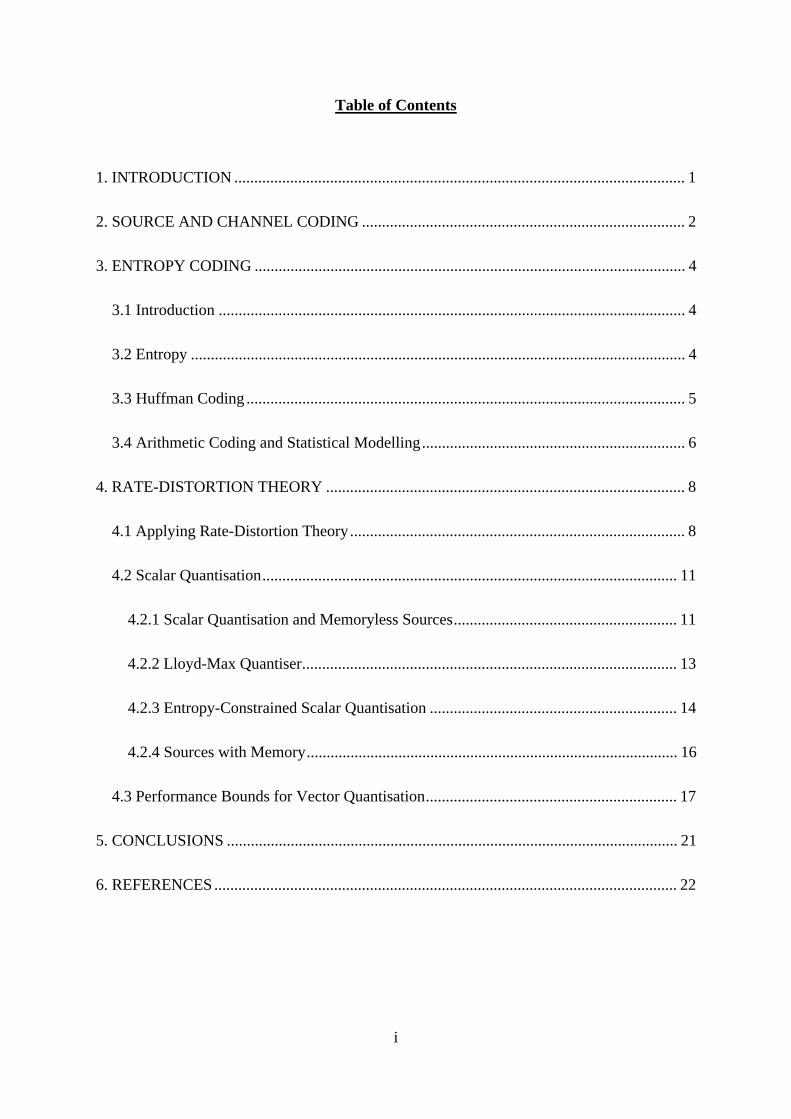
Image compression belongs to a more general category known as signal coding. The

foundations for signal coding are in information theory, which is the mathematical theory for

communication developed in the seminal work of Shannon (1948, 1959) (Cover and Thomas

1991). The representation for a communication system is shown in Figure 2-1. Shannon

(1948) distinguished between source coding, which provides an efficient digital

representation of the source signal, and channel coding, which is the error-control coding for

reliable communication over noisy channels.

SourceEncoder

ChannelEncoder Modulator

SourceDecoder

ChannelDecoder

Demodulator

Transmissionchannel or

storage device

SignalSource

Receiver

Source Coding Channel Coding

Figure 2-1: Block diagram of a digital communication system (adapted from Jayant et

al. (1993))

Shannon (1948) showed the important outcome that source coding and channel coding can be

designed separately without loss of optimality compared to a joint design (Berger 1971,

Section 3.3; Gray 1990, Section 2.1). This considerably simplifies the design of the

communication system. However, Shannon’s separation theorem is only valid in the limit of

infinitely long codes and for point-to-point, rather than broadcast, communication. For the

implementation of a practical system which has a noisy channel, techniques for channel-error

protection deserve special attention. Image coders are usually highly sensitive to channel

errors due to error propagation. The influence is more pronounced in highly efficient and

adaptive coders, where the corruption of the adaptive parameters can significantly alter the

reconstruction process. In such cases, joint source-channel coding is advantageous if

robustness and high-quality reconstructions are desirable (Jayant et al. 1993). A joint design

generally provides a better performance trade-off and lower overall implementation

3

complexity compared to a separate design (Ramchandran 1993, Chapter 6). An example of

joint source-channel coding is Zeger’s (1990) work on vector quantisers, which uses pseudo-

Gray coding for the assignment of codeword indices.

As with mainstream image-compression work, this thesis focusses on source coding with the

assumption of a noiseless channel (Gersho and Gray 1992, Chapter 1). For a noisy channel,

such a system may be suboptimal and unnecessarily complex compared to a jointly designed

system. However, a good overall system can still be expected by cascading two well-designed

source and channel coders (Blahut 1987). In other cases, noise-protection techniques such as

those described by Lam (1990) for entropy coding and quantisation can be incorporated. As

another example, for a transform-coding scheme, two approaches used are to dynamically

allocate bits between source and channel coding depending on the channel quality and to

perform error correction at the receiver (Clarke 1985, Chapter 8). Thus, although channel-

noise effects are an important consideration for practical communication systems, for image

coding, a noiseless channel is widely assumed, and this frees the system designer to

concentrate solely on source coding.

Source coding theory deals with the efficient representation of the data generated by an

information source (Gray 1990). For image coding, this is achieved by successfully exploiting

the redundancies of the image. The two fundamental concepts of source coding theory are

noiseless coding theory and rate-distortion or noisy coding theory. These two concepts are

discussed in the following sections.

4

3. ENTROPY CODING

3.1 Introduction

Noiseless source coding is concerned with the measure of information or data complexity and

the minimum average bit rate required for the lossless representation of the information.

Central to the theory is the concept of entropy and how lossless codes can be constructed

efficiently. Popular techniques that arose from noiseless coding theory are Huffman,

arithmetic, and Ziv-Lempel coding. Detailed information on this subject can be found in

books by Bell et al. (1990), Storer (1988), and Lynch (1985).

3.2 Entropy

Entropy is a measure of information content of an information source. Consider a discrete

information source S that has a finite alphabet { }A a aM= −0 1, ,� with marginal probability

mass function p(a) = pS(a). The average information provided by a symbol is the self-

information of its occurrence, which is defined as

( ) ( )[ ] ( )i a p a p ai i i= = −log log1 , (3-1)

where, unless stated otherwise, log(⋅) uses a base of 2. Entropy is the average amount of

information per source symbol. The first-order estimate of the source entropy considers only

individual symbols and can be defined as

( ) ( ) ( ) ( )H S p a I a p ai ii

M

ii

M

10

1

0

1= = −

=

−

=

−∑ ∑ log bits/symbol. (3-2)

When a block of k symbols are grouped together, the resulting source Sk is termed the k-th

extension of the source S and the k-th order entropy is Hk(Sk). The entropy of the source H(S)

is the resulting bits per symbol when k tends to infinity:

( ) ( )limk

kkH S H S

→∞= . (3-3)

5

According to Shannon’s noiseless source coding theorem, for any δ > 0 and a k large enough,

a code can be constructed such that the average number of bits per original source symbol L

satisfies

( ) ( )H S L H S≤ < + δ . (3-4)

Thus, a source can be losslessly coded with an average bit rate arbitrarily close to, but not less

than, the source entropy H(S). Note that in practice, the true entropy of a source can be

impractical to measure since the calculation quickly becomes intractable for large k. For

sources with short-term memory, however, H(S) can be closely estimated with small values of

k.

For a source with continuous amplitude, the absolute entropy defined in Eq. (3-2) is infinite.

Assuming that the random variable X has probability density function (pdf) fX, the meaningful

entropy measure for such a source is the differential entropy defined as

( ) ( ) ( )h X f x f x dxX Xx

= −∫ log . (3-5)

3.3 Huffman Coding

Two of the methods to realise the ideal of the noiseless coding theorem are permutation

coding (Berger 1982) and entropy coding. Permutation coding uses fixed-length codes but has

the disadvantage that the codewords can be very long, which also introduces delays. Entropy

coding, the more popular method, uses variable-lengths codes with a procedure that assigns

shorter codewords to more probable outcomes, and vice versa. A practical method for

constructing compact codes is provided by Huffman (1952), and this method is widely used

due to its speed and good compaction performance (Nelson 1992, Chapter 3).

For a source with an alphabet of size M, Huffman coding is performed by repeatedly

combining the two least-probable symbols so that the original source is reduced at each stage.

For each pairing, the new symbol is assigned the probability of the two old symbols

combined. This procedure is repeated until the source is reduced to only two symbols, which

are assigned the codewords “0” and “1” . The codewords for the previous reduced stage can

now be constructed by appending a “0” or “1” to the codeword of the two least probable

symbols. This is repeated until each symbol has been assigned a codeword.

6

Although it has a simple and fast implementation, Huffman coding has a number of serious

limitations (Rabbani and Jones 1991, Chapter 3). Since its codeword lengths are integers,

optimal performance is only possible if all the symbol probabilities are integral powers of

two, which is rare in practice. The worst case is realised when a source has a symbol whose

probability approaches unity. The resulting bit rate is approximately 1 bit/symbol even though

its entropy is much less. This limitation also means that Huffman coding is inefficient for a

binary source since each symbol must be coded with at least 1 bit, regardless of the source

probability distribution.

The second limitation is that Huffman coding does not adapt well to changing source

statistics if fixed Huffman tables are used. One solution is to use a two-pass algorithm where

the symbols statistics are first gathered to generate the Huffman tables, and the data are

encoded in the second pass (Nelson 1992, Chapter 3). The disadvantages with this method are

the overhead cost in transmitting the table and the inability to adapt to short-term statistics

since a static Huffman code is used. Dynamic or adaptive Huffman coding has been proposed

to overcome this (Knuth 1985; Nelson 1992, Chapter 4), but it incurs a complexity cost.

3.4 Arithmetic Coding and Statistical Modelling

The basic concept for arithmetic coding can be attributed to Elias in the early 1960’s but the

first practical methods were proposed by Rissanen (1976) and Pasco (1976). A widely used

implementation is the adaptive coder proposed by Witten et al. (1987).

Unlike Huffman coding, arithmetic coding does not assign particular bit patterns to the source

symbols. Instead, a single arithmetic codeword is assigned to the complete sequence of

symbols. Arithmetic codewords consist of sub-intervals of the unit interval [0, 1). They are

specified with sufficient bits to differentiate each sub-interval corresponding to a source

symbol from other possible sub-intervals. Shorter codes are assigned to larger sub-intervals or

more probable symbols. As the coding proceeds, the sub-intervals are refined, and bits are

output as they are determined.

The main advantages of arithmetic coding are its optimality in approaching the entropy limit

and its inherent separation of modelling and coding (Howard and Vitter 1994). Since

arithmetic coding does not translate each symbol to an integral number of bits, theoretically it

can approach the lower entropy bound of Eq. (3-4) arbitrarily closely.

7

The decoupling of modelling and coding means that an arbitrarily complex source modeller

can be used without changing the coder (Rissanen and Langdon 1981). Since the arithmetic

coder will be optimal to the entropy of the source model, significant coding gains are possible

through accurate prediction of source probabilities. Statistical models can be divided into

fixed models and dynamic models, which can adapt to the short-term statistics of the source.

One method of collecting statistics for a fixed model is by analysing a set of training data.

Another method is the two-pass method described in Section 3.3. Unlike the two-pass

method, which requires the model to be sent as overhead data, dynamic modelling refines the

model as the coding proceeds. A common method is to update a frequency table of symbols

that have already been coded. When coding a relatively short data stream, dynamic modelling

can be improved by presetting the frequency tables with fixed-model statistics. Larger block

sizes and conditional modelling can also be applied for both techniques (Pennebaker and

Mitchell 1993, Chapter 8). Compared to arithmetic coding, Huffman coding is not as easily

modified for highly complex modellers. For example, Huffman coding using a dynamic

model is significantly slower than one that uses a fixed model (Nelson 1992, Appendix A).

Current research in arithmetic coding generally deals with efficient modelling of the source

(eg. Duttweiler and Chamzas 1995) and faster implementations (eg. Lei 1994). Arithmetic

coding is commonly used at the lossless-coding stage of image compression. For example,

one of the lossless coders specified in the JPEG standard is IBM’ s binary arithmetic coder,

QM-Coder (Pennebaker and Mitchell 1993, Chapter 9). For image coding applications,

arithmetic and Huffman coding have often been selected in preference to dictionary-based

schemes such as LZ77 and LZ78 (Nelson 1992, Chapter 7). The former class generally

outperforms the latter for sources with low-order dependency (Gray et al. 1995). In Chang et

al. (1992)’s experiment with JPEG compression of grayscale images, arithmetic coding

approximately outperformed Huffman coding by 7% and LZ78 coding by 9%.

8

4. RATE-DISTORTION THEORY

4.1 Applying Rate-Distortion Theory

Rate-distortion (R-D) theory is one of the fundamental concepts of source-coding theory. It

relates the trade-off between rate and distortion in a coding system and provides upper and

lower bounds for the average bit rate when coding subject to a fidelity criterion. More

specifically, the rate-distortion function R(D) specifies the minimum average rate R needed to

ensure that the average distortion does not exceed a given value D. An alternate interpretation

is the distortion-rate function D(R), which specifies the minimum average distortion D given

the average rate R. Following the development of rate-distortion theory by Shannon (1959),

Gallager (1968, Chapter 9) was the first to describe a general theory for evaluating rate-

distortion functions, and the theory was extended by Berger (1971).

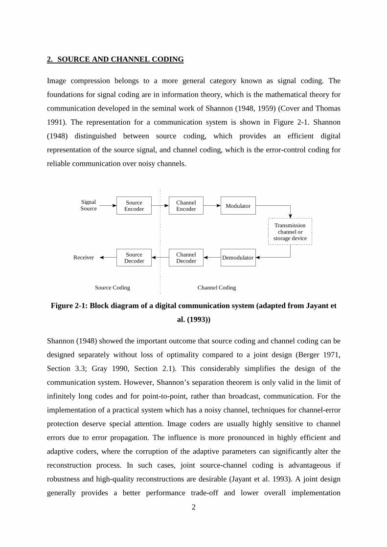
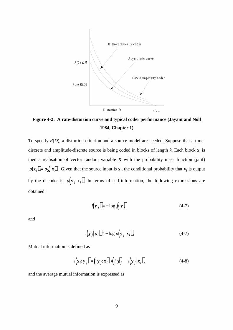
It can be shown that R(D) is a convex and monotonically non-increasing function of D (Gray

1990, Section 4.1). A typical rate-distortion curve for a discrete source is shown in Figure 4-2

, labelled as “asymptotic curve.” Based on the given rate and distortion definitions, this bound

represents the best theoretical R-D performance an encoder can achieve in coding the source.

R(0) specifies the minimum rate required to achieve distortion-free coding of the source.

Depending on the distortion function, it is less than or equal to the entropy of the source. For

very low bit rates, the distortion approaches a maximum value Dmax. In the case of a discrete

source, this is the variance of the signal.

The performance of an encoder depends on how well it can model the source statistics.

Figure 4-2 also shows the hypothetical R-D curves for a high-complexity and a low-

complexity coder. As expected, a more sophisticated coder generally achieves a higher R-D

performance compared to that of a simpler one.

9

D istorti on D

Rate R(D )

D m ax

H igh-complex ity coder

L ow -complex ity coder

A sy mptoti c curveR(0) ≤ H

Figure 4-2: A rate-distortion curve and typical coder performance (Jayant and Noll

1984, Chapter 1)

To specify R(D), a distortion criterion and a source model are needed. Suppose that a time-

discrete and amplitude-discrete source is being coded in blocks of length k. Each block xi is

then a realisation of vector random variable X with the probability mass function (pmf)

( ) ( )p pi ix xX= . Given that the source input is xi, the conditional probability that yj is output

by the decoder is ( )p j iy x . In terms of self-information, the following expressions are

obtained:

( ) ( )i pj jy y= − log (4-7)

and

( ) ( )i pj i j iy x y x= − log . (4-7)

Mutual information is defined as

( ) ( ) ( ) ( )i i i ii j j i j j ix y y x y y x; ;= = − , (4-8)

and the average mutual information is expressed as

10

( ) ( ) ( )( )I p

p

pi j i j

j i

jji

x y x yy x

y; , log= ∑∑ . (4-9)

Let ( )d i jx y, be the distortion between xi and yj. Then the average distortion per source

symbol is

( ) ( ) ( )D p dp i j i j

jij iy x

x y x y= ∑∑ , , . (4-10)

The k-block rate-distortion function is then defined as

( )( )

( )R Dk

IkD D

i jp j i

=<

min ;y x

x y1

(4-11)

Rk(D) is monotonically non-increasing as a function of k (Makhoul 1985), and this

characteristic has been seen as a motivation for block coding or vector quantisation. The

limiting value of Rk(D) is known as the rate-distortion function:

( ) ( )R D R Dk

k=→∞lim . (4-12)

The problem of finding R(D) can be approached analytically for memoryless and Markov

sources and single-letter distortion measures (Gray 1990, Chapter 3). R-D theory has also

been extended to stationary ergodic processes with discrete alphabets and to Gaussian

processes, as well as to stationary and abstract alphabets (Gray 1990, Chapter 3). For cases

where a closed-form solution does not exist, the numerical technique discovered

independently by Arimoto (1972) and Blahut (1972) can be employed.

A number of difficulties have been encountered with applying rate-distortion theory to

practical use in image coding (Netravali and Limb 1980). First, it should be recognised that

the theory is for specifying performance bounds rather than on the construction of coders that

can attain such bounds. Second, it is difficult to find good statistical model for images, and

the source models used in rate-distortion theory do not reflect the characteristic of natural

imagery being non-Gaussian, non-stationary, and having complex power spectra (Jayant et al.

1993; Netravali and Haskell 1988, Chapter 3). Even if these properties can be modelled

accurately, the calculation of the rate-distortion function is complex and can be intractable

11

(Rosenfeld and Kak 1982, p. 194). However, it should be pointed out that data such as

subband and transform coefficients can be modelled accurately with well-behaved pdf’s, as

discussed in 4.2.1.

Perhaps the most serious difficulty with applying R-D theory is the lack of a distortion

measure that is both perceptually meaningful and analytically tractable (Jayant et al. 1993).

The commonly used single-letter distortion measure, such as mean-square error, does not

correlate well with perceived image quality (Girod 1993). Although, a large number of

perceptual image quality metrics have been proposed, as yet, there has been no de facto

standard, and many of them are multiple-letter rather than single-letter distortion measures

(Eskicioglu 1995a).

Nevertheless, rate-distortion theory provides a theoretical framework for quantifying the

trade-offs and providing performance limits when coding subject to a fidelity criterion. Some

of the main applications of rate-distortion theory relevant to image coding are design of scalar

and vector quantisers; determining performance gains of coding systems; and bit allocation.

The first application, where rate-distortion theory is directly used to provide the performance

bounds for scalar and vector quantisers, is discussed in the following sections. In the second

application, R-D theory is useful for comparing different transformations and coding

schemes. Such analysis can lead to the derivation of the coding gain, which quantifies the

advantage of quantising the transformed signal compared to quantising the original signal.

For the third application, knowledge of the system’s R(D) functions is necessary for optimal

bit allocation. However, R-D theory is not used directly to derive the bit-allocation

algorithms. Coding gain and bit allocation are discussed in Chapter 3.

4.2 Scalar Quantisation

4.2.1 Scalar Quantisation and Memoryless Sources

Much research has been done in the area of scalar quantisation, and an introduction and

historical review can be found in Gersho (1978). Jayant and Noll (1984, Chapter 4) and

Clarke (1985, Chapter 4) provide detailed reviews of the important results of quantisation

research. The discussion here summarises the performance bounds derived from rate-

distortion theory and the commonly used Lloyd-Max quantiser and entropy-constrained

uniform quantiser.

12

A scalar quantiser maps a set of input values or a continuous function into a smaller, finite

number of output levels. More specifically, an N-point scalar quantiser Q can be defined as a

mapping Q:R C→ , where R is the set of real numbers and the output set or codebook C of

size N is defined as

( )C R= = ⊂y i Ni ; ,2, ,1 � . (4-13)

The quantiser mapping Q can be decomposed into the encoder mapping E R I: → and

decoder mapping D I R: → , where I is the index set and the quantiser-cell i ndex is

represented as { }i N∈ =I 1,2, ,� . Given an input value x ∈ R, E will output the value i if x

falls into the interval

{ }I i i ix x x i N: ; ,2, ,< ≤ =+1 1 � . (4-14)

The values xk thus define the boundaries of the intervals and specify the decision levels of the

quantiser. Given a value i, D outputs the reconstruction value yi. The granular region of the

quantiser is the range (x1, xN], and values outside this range are in the overload region.

Rate-distortion theory has been successfully applied to determining the performance bounds

of scalar quantisers for memoryless sources with well-defined distributions.

An often quoted result is the R(D) function derived by Shannon (1959) for a memoryless

zero-mean Gaussian source with variance σ2 and a mean-square error (MSE) distortion:

( )R D D D

DG =

≤ <

≤

12

log σ σ

σ

2 2

2

0

0

. (4-15)

Since a Gaussian density has the maximum differential entropy, this is the upper R(D) bound

for other memoryless densities (Jayant and Noll 1984, Appendix D). Their lower bounds can

be determined by (Clarke 1985, Chapter 9)

( ) ( )R D h eDL = ⋅ − 12

2log π , (4-16)

13

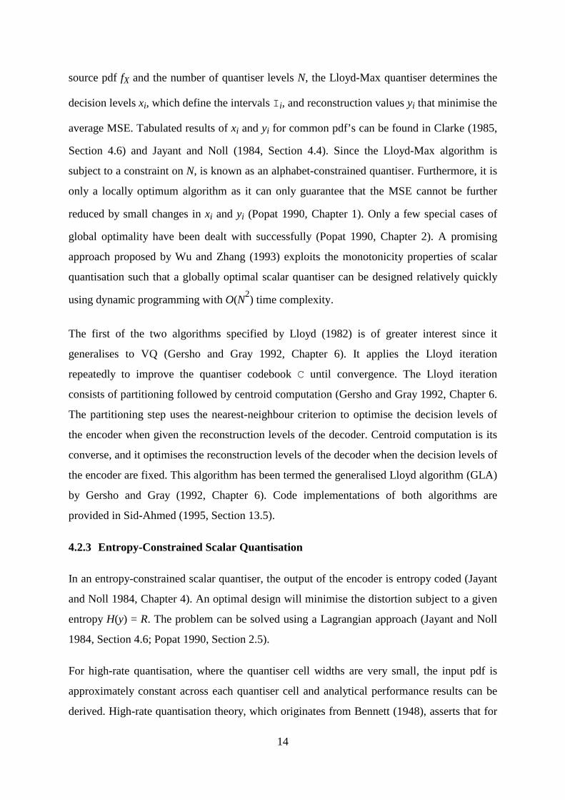
where h(⋅) is the differential entropy of the pdf. Column 2 of Table 4-1 shows h(⋅) for

different pdf’s (Makhoul et al. 1985). Column 3 shows the difference between the upper and

lower bounds. The signal-to-noise ratio (SNR) can be calculated as

SNR dB= 10 10

2log

σD

(4-17)

and the results are shown on Column 4. It can be observed that the Gamma density exhibits

the greatest deviation from the Gaussian as it is the most peaked of the four pdf’s. Note that

the lower bounds for non-Gaussian densities are optimistic for low bit rates (Jayant and Noll

1984, Appendix D). At such rates, more accurate bounds are obtained using the Arimoto-

Blahut algorithm (Arimoto 1972; Blahut 1972), as shown by Noll and Zelinski (1978) .

This analysis is of practical use since coefficients related to the coding of real-world signals

can be well-modelled by such pdf’s. The Gamma density has been proposed as a good model

for long-term speech statistics, and the Gaussian pdf for short-term statistics (Jayant and Noll

1984, Chapter 2). The pdf of the predicted coefficients is well matched with a Laplacian

distribution (Rabbani and Jones 1991, Chapter 7) and so are transform and subband

coefficients, although the generalised Gaussian density can provide a slightly more accurate

match (Birney and Fischer 1995).

pdf h(⋅) RG(D) - RL(D)

(bits)

SNRL(R) - SNRG(R)

(dB)

RG(D) - RL(D)

(bits)

SNRL(R) - SNRG(R)

(dB)

Gaussian ( )12

22log π σe0 0 0.722 4.35

Uniform ( )12

212log σ 0.255 1.53 0.255 1.53

Laplacian ( )12

2 22log e σ 0.104 0.63 1.190 7.17

Gamma ( )12

1 24 3log π σe C−

C = Euler’s constant

0.709 4.27 1.963 11.82

Table 4-1: Rate-distortion bounds for four common pdf's (adapted from Makhoul et al.

1985)

4.2.2 Lloyd-Max Quantiser

The last two columns of Table 4-1 show the performance differences between the well-known

Lloyd-Max quantiser (Lloyd 1982; Max 1960) and the Shannon lower bound. Given the

14

source pdf fX and the number of quantiser levels N, the Lloyd-Max quantiser determines the

decision levels xi, which define the intervals I i, and reconstruction values yi that minimise the

average MSE. Tabulated results of xi and yi for common pdf’ s can be found in Clarke (1985,

Section 4.6) and Jayant and Noll (1984, Section 4.4). Since the Lloyd-Max algorithm is

subject to a constraint on N, is known as an alphabet-constrained quantiser. Furthermore, it is

only a locally optimum algorithm as it can only guarantee that the MSE cannot be further

reduced by small changes in xi and yi (Popat 1990, Chapter 1). Only a few special cases of

global optimality have been dealt with successfully (Popat 1990, Chapter 2). A promising

approach proposed by Wu and Zhang (1993) exploits the monotonicity properties of scalar

quantisation such that a globally optimal scalar quantiser can be designed relatively quickly

using dynamic programming with O(N2) time complexity.

The first of the two algorithms specified by Lloyd (1982) is of greater interest since it

generalises to VQ (Gersho and Gray 1992, Chapter 6). It applies the Lloyd iteration

repeatedly to improve the quantiser codebook C until convergence. The Lloyd iteration

consists of partitioning followed by centroid computation (Gersho and Gray 1992, Chapter 6.

The partitioning step uses the nearest-neighbour criterion to optimise the decision levels of

the encoder when given the reconstruction levels of the decoder. Centroid computation is its

converse, and it optimises the reconstruction levels of the decoder when the decision levels of

the encoder are fixed. This algorithm has been termed the generalised Lloyd algorithm (GLA)

by Gersho and Gray (1992, Chapter 6). Code implementations of both algorithms are

provided in Sid-Ahmed (1995, Section 13.5).

4.2.3 Entropy-Constrained Scalar Quantisation

In an entropy-constrained scalar quantiser, the output of the encoder is entropy coded (Jayant

and Noll 1984, Chapter 4). An optimal design will mi nimise the distortion subject to a given

entropy H(y) = R. The problem can be solved using a Lagrangian approach (Jayant and Noll

1984, Section 4.6; Popat 1990, Section 2.5).

For high-rate quantisation, where the quantiser cell widths are very small, the input pdf is

approximately constant across each quantiser cell and analytical performance results can be

derived. High-rate quantisation theory, which originates from Bennett (1948), asserts that for

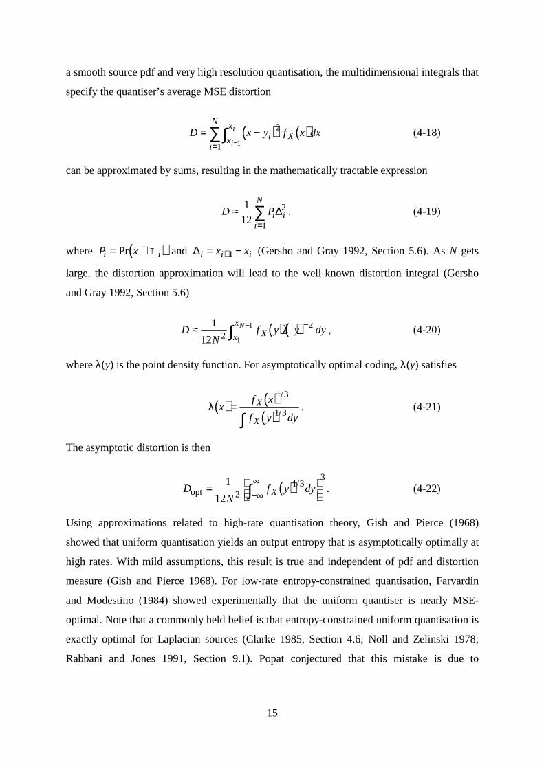
15

a smooth source pdf and very high resolution quantisation, the multidimensional integrals that

specify the quantiser’s average MSE distortion

( ) ( )D x y f x dxi Xx

x

i

N

i

i= −−

∫∑=

2

1 1(4-18)

can be approximated by sums, resulting in the mathematically tractable expression

D Pi ii

N≈

=∑1

122

1

∆ , (4-19)

where ( )P xi i= ∈Pr I and ∆i i ix x= −+1 (Gersho and Gray 1992, Section 5.6). As N gets

large, the distortion approximation will l ead to the well-known distortion integral (Gersho

and Gray 1992, Section 5.6)

( ) ( )DN

f y y dyXx

xN≈ −−∫1

12 22

1

1 λ , (4-20)

where λ(y) is the point density function. For asymptotically optimal coding, λ(y) satisfies

( ) ( )( )

λ xf x

f y dy

X

X

=∫

1 3

1 3

/

/. (4-21)

The asymptotic distortion is then

( )DN

f y dyXopt =

−∞

∞∫1

12 21 3

3/ . (4-22)

Using approximations related to high-rate quantisation theory, Gish and Pierce (1968)

showed that uniform quantisation yields an output entropy that is asymptotically optimally at

high rates. With mild assumptions, this result is true and independent of pdf and distortion

measure (Gish and Pierce 1968). For low-rate entropy-constrained quantisation, Farvardin

and Modestino (1984) showed experimentally that the uniform quantiser is nearly MSE-

optimal. Note that a commonly held belief is that entropy-constrained uniform quantisation is

exactly optimal for Laplacian sources (Clarke 1985, Section 4.6; Noll and Zelinski 1978;

Rabbani and Jones 1991, Section 9.1). Popat conjectured that this mistake is due to

16

misinterpretation of Berger’s (1972) results and showed that a non-uniform quantiser results

in lower distortion, although the difference is not significant.

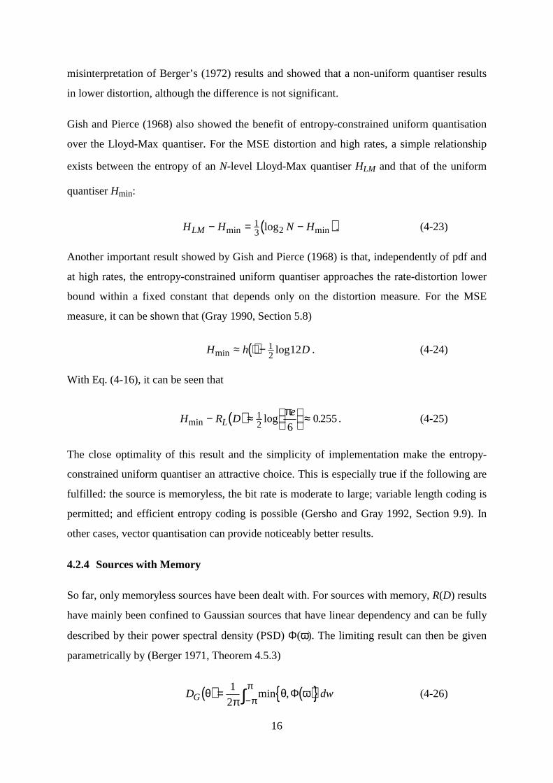
Gish and Pierce (1968) also showed the benefit of entropy-constrained uniform quantisation

over the Lloyd-Max quantiser. For the MSE distortion and high rates, a simple relationship

exists between the entropy of an N-level Lloyd-Max quantiser HLM and that of the uniform

quantiser Hmin:

( )H H N HLM − = −min minlog13 2 . (4-23)

Another important result showed by Gish and Pierce (1968) is that, independently of pdf and

at high rates, the entropy-constrained uniform quantiser approaches the rate-distortion lower

bound within a fixed constant that depends only on the distortion measure. For the MSE

measure, it can be shown that (Gray 1990, Section 5.8)

( )H h Dmin log≈ ⋅ − 12

12 . (4-24)

With Eq. (4-16), it can be seen that

( )H R De

Lmin log .− ≈

≈1

2 60 255

π. (4-25)

The close optimality of this result and the simplicity of implementation make the entropy-

constrained uniform quantiser an attractive choice. This is especially true if the following are

fulfilled : the source is memoryless, the bit rate is moderate to large; variable length coding is

permitted; and efficient entropy coding is possible (Gersho and Gray 1992, Section 9.9). In

other cases, vector quantisation can provide noticeably better results.

4.2.4 Sources with Memory

So far, only memoryless sources have been dealt with. For sources with memory, R(D) results

have mainly been confined to Gaussian sources that have linear dependency and can be fully

described by their power spectral density (PSD) Φ(ω). The limiting result can then be given

parametrically by (Berger 1971, Theorem 4.5.3)

( ) ( ){ }D dwG θπ

θ ωπ

π=

−∫1

2min ,Φ (4-26)

17

( ) ( )R dwG θ

πω

θππ

=

−∫

1

20

1

2 2max , logΦ

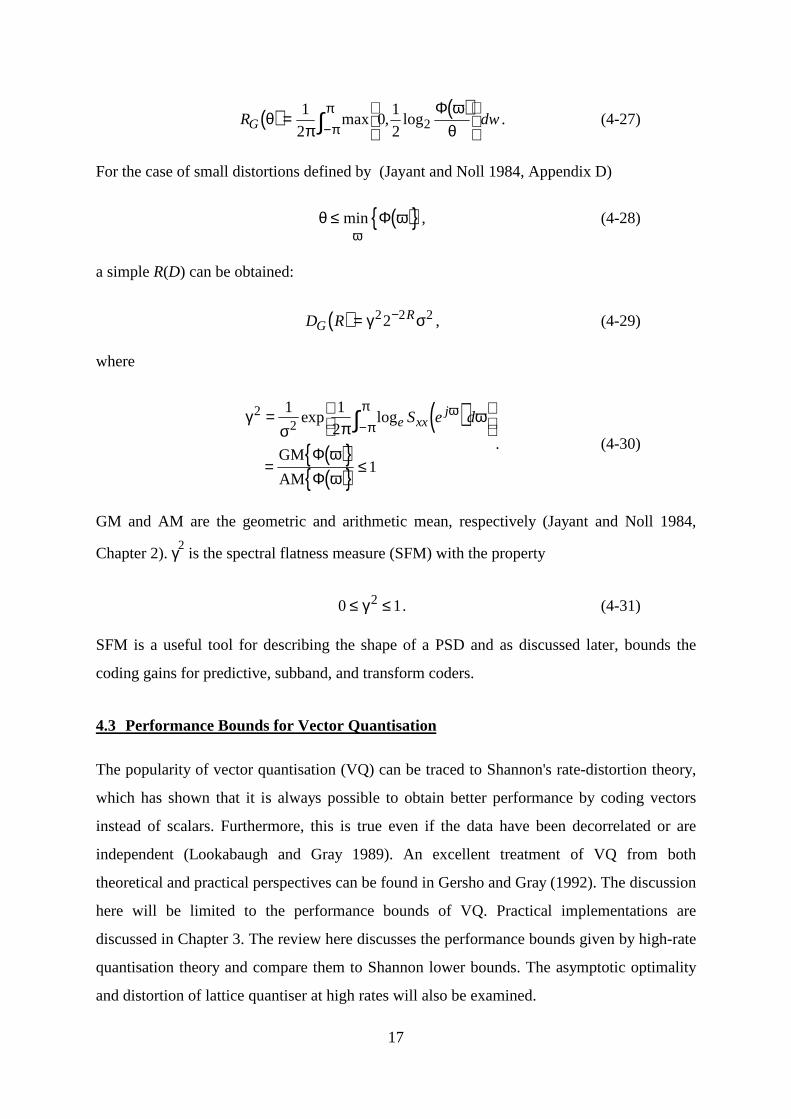
. (4-27)

For the case of small distortions defined by (Jayant and Noll 1984, Appendix D)

( ){ }θ ωω

≤ min Φ , (4-28)

a simple R(D) can be obtained:

( )D RGR= −γ σ2 2 22 , (4-29)

where

( )( ){ }( ){ }

γσ π

ω

ωω

ωπ

π22

1 12

1

=

= ≤

−∫exp loge xxjS e d

GM

AM

ΦΦ

. (4-30)

GM and AM are the geometric and arithmetic mean, respectively (Jayant and Noll 1984,

Chapter 2). γ2 is the spectral flatness measure (SFM) with the property

0 12≤ ≤γ . (4-31)

SFM is a useful tool for describing the shape of a PSD and as discussed later, bounds the

coding gains for predictive, subband, and transform coders.

4.3 Performance Bounds for Vector Quantisation

The popularity of vector quantisation (VQ) can be traced to Shannon's rate-distortion theory,

which has shown that it is always possible to obtain better performance by coding vectors

instead of scalars. Furthermore, this is true even if the data have been decorrelated or are

independent (Lookabaugh and Gray 1989). An excellent treatment of VQ from both

theoretical and practical perspectives can be found in Gersho and Gray (1992). The discussion

here will be limited to the performance bounds of VQ. Practical implementations are

discussed in Chapter 3. The review here discusses the performance bounds given by high-rate

quantisation theory and compare them to Shannon lower bounds. The asymptotic optimality

and distortion of lattice quantiser at high rates will also be examined.

18

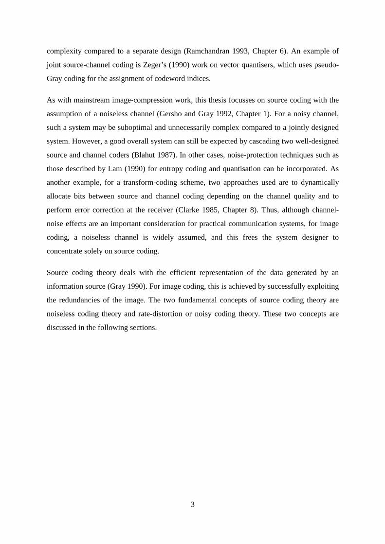
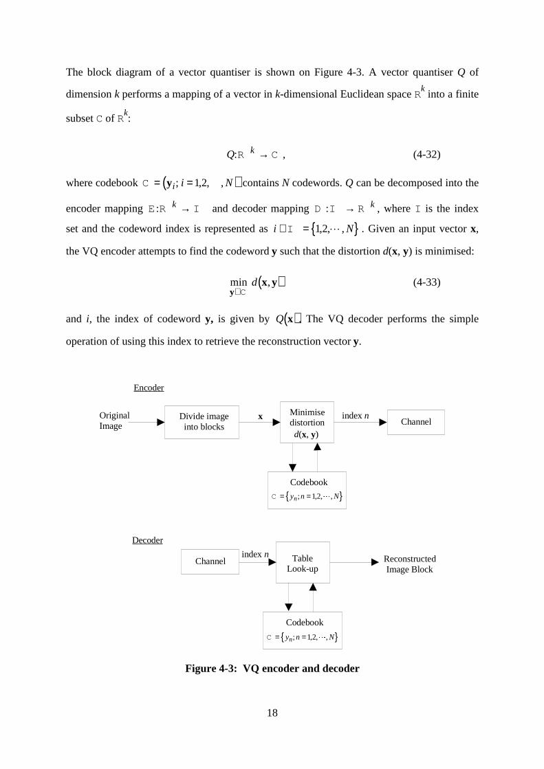
The block diagram of a vector quantiser is shown on Figure 4-3. A vector quantiser Q of

dimension k performs a mapping of a vector in k-dimensional Euclidean space Rk into a finite

subset C of Rk:

Q k:R C→ , (4-32)

where codebook ( )C = =yi i N; ,2, ,1 � contains N codewords. Q can be decomposed into the

encoder mapping E R I: k → and decoder mapping D I R: → k , where I is the index

set and the codeword index is represented as { }i N∈ =I 1,2, ,� . Given an input vector x,

the VQ encoder attempts to find the codeword y such that the distortion d(x, y) is minimised:

( )min ,y

x y∈C

d (4-33)

and i, the index of codeword y, is given by ( )Q x . The VQ decoder performs the simple

operation of using this index to retrieve the reconstruction vector y.

Codebook

Minimise distortion

OriginalImage

Divide image into blocks Channel

index nx

Encoder

Channel Table Look-up

Codebook

ReconstructedImage Block

Decoder

index n

d(x, y)

{ }C = =y n Nn; , , ,1 2�

{ }C = =y n Nn; , , ,1 2�

Figure 4-3: VQ encoder and decoder

19

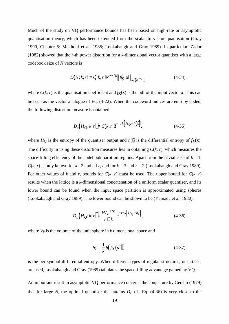
Much of the study on VQ performance bounds has been based on high-rate or asymptotic

quantisation theory, which has been extended from the scalar to vector quantisation (Gray

1990, Chapter 5; Makhoul et al. 1985; Lookabaugh and Gray 1989). In particular, Zador

(1982) showed that the r-th power distortion for a k-dimensional vector quantiser with a large

codebook size of N vectors is

( ) ( ) ( ) ( )D N k r C k r N fr kk k r

; ; , /= −+X x , (4-34)

where C(k, r) is the quantisation coefficient and fX(x) is the pdf of the input vector x. This can

be seen as the vector analogue of Eq. (4-22). When the codeword indices are entropy coded,

the following distortion measure is obtained

( ) ( ) ( )[ ]D H k r C k re Qr k H hQ; ; ,/=

− − ⋅2 , (4-35)

where HQ is the entropy of the quantiser output and h(⋅) is the differential entropy of fX(x).

The difficulty in using these distortion measures lies in obtaining C(k, r), which measures the

space-filling efficiency of the codebook partition regions. Apart from the trivial case of k = 1,

C(k, r) is only known for k =2 and all r, and for k = 3 and r = 2 (Lookabaugh and Gray 1989).

For other values of k and r, bounds for C(k, r) must be used. The upper bound for C(k, r)

results when the lattice is a k-dimensional concatenation of a uniform scalar quantiser, and its

lower bound can be found when the input space partition is approximated using spheres

(Lookabaugh and Gray 1989). The lower bound can be shown to be (Yamada et al. 1980):

( ) [ ]D H k rkV

r keL Q

kr k r k H hQ k; ;/ /=

+

− − −, (4-36)

where Vk is the volume of the unit sphere in k dimensional space and

( )( )hk

h fk = 1X x (4-37)

is the per-symbol differential entropy. When different types of regular structures, or lattices,

are used, Lookabaugh and Gray (1989) tabulates the space-filling advantage gained by VQ.

An important result in asymptotic VQ performance concerns the conjecture by Gersho (1979)

that for large N, the optimal quantiser that attains DL of Eq. (4-36) is very close to the

20

uniform quantiser. Such a quantiser is known as the lattice quantiser and its codebook points

form a regularly spaced array of points in k-dimensional space (Conway and Sloane 1988). A

major advantage of a lattice quantiser is its efficient encoding algorithm. Due to the regularity

of its codebook partitions, a vector can be encoded without the slow nearest-neighbour search

of conventional VQ. The asymptotic optimality of the lattice quantiser is discussed in Gray

(1990, Section 5.6) and can be seen as a generalisation of Gish and Pierce’s results (1968) to

vector coding. Furthermore, due to its regular structure, the asymptotic average distortion,

rather than just the lower bound, of a lattice quantiser can be obtained (Gray 1990, Section

5.5).

High-rate quantisation theory has also been used to quantify the performance gains of VQ

over scalar quantisation. Lookabaugh and Gray (1989) decomposed the coding gain into three

components: the space-filling, shape, and memory advantages.

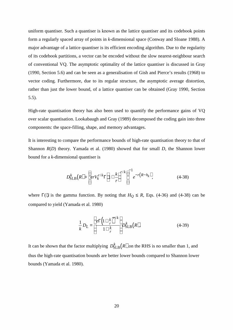
It is interesting to compare the performance bounds of high-rate quantisation theory to that of

Shannon R(D) theory. Yamada et al. (1980) showed that for small D, the Shannon lower

bound for a k-dimensional quantiser is

( ) ( )D R erVk

rek

kr k

r kr R hk

SLB = +

−− −/

/Γ 1

1

, (4-38)

where Γ(⋅) is the gamma function. By noting that HQ ≤ R, Eqs. (4-36) and (4-38) can be

compared to yield (Yamada et al. 1980)

( ) ( )1 1

1kD

eD RL

kr

r k

kr

k=+

+

Γ/

SLB . (4-39)

It can be shown that the factor multiplying ( )D RkSLB on the RHS is no smaller than 1, and

thus the high-rate quantisation bounds are better lower bounds compared to Shannon lower

bounds (Yamada et al. 1980).

21

5. CONCLUSIONS

In information theory, the main domains of interest are noiseless coding theory and rate-

distortion or noisy coding theory, although practical implementations should also consider

channel coding, as pointed out in Section 2. In Section 3, the two popular forms of noiseless

coding, Huffman and arithmetic coding, are reviewed and constrasted. The advantages of

arithmetic coding are its asymptotic optimality in approach the source entropy and its

separation of source modelling and symbol coding.

The discussion on rate-distortion theory concentrated on finding performance bounds for

scalar and vector quantisation, with recent progress in both fields highlighted. The widely

used Lloyd-Max quantiser and entropy-constrained scalar quantisation were also discussed.

Following this, two methods of finding performance bounds in vector quantisation are

described. It is shown that high-rate quantisation bounds is an improvement over the Shannon

lower bound. An important observation is the difficulties in applying rate-distortion theory to

practical image coding methods and image models.

22

6. REFERENCES

1. Arimoto, S. (1972). An algorithm for computing the capacity of arbitrary discrete

memoryless channels. IEEE Transactions on Information Theory, IT-18(1), 14-20.

2. Bell, T.C., Cleary, J.G. and Witten, I.H. (1990). Text compression. Prentice-Hall,

Englewood Cliffs, NJ.

3. Bennett, W.R. (1948). Spectra of quantised signals. Bell Systems Technical Journal, 27,

Jul, 446-72.

4. Berg, A.P. and Mikhael, W.B. (1994). Survey of techniques for lossless compression of

signals. Midwest Symposium on Circuits and Systems, 2, 943-6.

5. Berger, T. (1971). Rate distortion theory: a mathematical basis for data compression.

Prentice-Hall, NJ.

6. Berger, T. (1972). Optimum quantisers and permutation codes. IEEE Transactions on

Information Theory, IT-18(6), 759-65.

7. Berger, T. (1982). Minimum entropy quantisers and permutation codes. IEEE

Transactions on Information Theory, IT-14(2), 149-56.

8. Birney, K.A., and Fischer, T.R. (1995). On the modeling of DCT and subband image

data for compression. IEEE Transactions on Image Processing, 4(2), 186-93.

9. Blahut, R.E. (1972). Computation of channel capacity and rate distortion functions.

IEEE Transactions on Information Theory, IT-18(4), 460-73.

10. Blahut, R.E. (1987). Principles and practice of information theory. Addison-Wesley,

Reading, MA.

11. Chang, M., Langdon, Jr., G. G., and Murphy, J. L. (1992). Compression gain aspects of

JPEG image compression. Proceedings of the SPIE, 1657, 159-68.

12. Clarke, R.J. (1985). Transform coding of images. Academic Press, London.

23

13. Conway, J.H. and Sloane, N.J.A. (1988). Sphere packings, lattices, and groups.

Springer-Verlag, New York, NY.

14. Cosman, P.C., Oehler, K.L., Riskin, E.A., and Gray, R.M. (1993). Using vector

quantisation for image processing. Proceedings of the IEEE, 81(9), 1326-41.

15. Cover, T.M. and Thomas, J.A. (1991). Elements of information theory. Wiley, New

York, NY.

16. Davisson, L. (1972). Rate distortion theory and application. Proceedings of the IEEE,

60(7), 800-8.

17. Dertouzos, M.L. (1991). Communications, computers and networks. Scientific

American, September, 30-7.

18. Duttweiler, D.L. and Chamzas, C. (1995). Probability estimation in arithmetic and

adaptive-huffman entropy coders. IEEE Transactions on Image Processing, 4(3), 237-

46.

19. Elias, P. (1963). In Abramson, N. Information Theory and Coding. McGraw-Hill, New

York, NY.

20. Eskicioglu, A.M. (1995a). State of the art in quality measurement of monochrome

compressed images. Submitted to Proceedings of the IEEE.

21. Farvardin, N. and Modestino, J.W. (1984). Optimum quantiser performance for a class

of non-Gaussian memoryless sources. IEEE Transactions on Information Theory, IT-

30(3), 485-97.

22. Gallager, R.G. (1968). Information theory and realiable communication. John Wiley &

Sons, New York, NY.

23. Gersho, A. (1978). Principles of quantisation. IEEE Transactions on Circuits and

Systems, CAS-25(7), 427-36.

24. Gersho, A. (1979). Asymptotically optimal block quantisation. IEEE Transactions on

Information Theory, IT-25(4), 373-80.

24

25. Gersho, A. and Gray, R.M. (1992). Vector quantisation and signal compression.

Kluwer Academic Publishers, Boston, MA.

26. Girod, B. (1993). What’s wrong with mean-squared error, in Watson, A.B. (ed.) Digital

images and human vision, 207-20. MIT Press, Cambridge, MA.

27. Gish, H. and Pierce, J.N. (1968). Asymptotically efficient quantising. IEEE

Transactions on Information Theory, IT-14(5), 676-83.

28. Gonzalez, R.C. and Woods, R.E. (1992). Digital image processing. 3rd ed. Addison-

Wesley, Reading, MA.

29. Gray, R.M. (1984). Vector quantisation. IEEE ASSP Magazine, 1, 4-29.

30. Gray, R.M. (1990). Source coding theory. Kluwer Academic Publishers, Boston, MA.

31. Howard, P.G. and Vitter, J.S. (1994). Arithmetic coding for data compression.

Proceedings of the IEEE, 82(6), 857-65.

32. Huang, J.-Y. and Schultheiss, P.M. (1963). Block quantisation of correlated Gaussian

random variables. IEEE Transactions on Communications, COM-11, Sep, 289-96.

33. Huffman, D.A. (1952). A method for the construction of minimum-redundancy codes.

Proceedings of the IRE, 40(9), 1098-101.

34. Jayant, N., Johnston, J., and Safranek, R. (1993). Signal compression based on models

of human perception. Proceedings of the IEEE, 81(10), 1385-422.

35. Jayant, N.S. and Noll, P. (1984). Digital coding of waveforms. Prentice-Hall,

Englewood Cliffs, NJ.

36. Knuth, D.E. (1985). Dynamic Huffman coding. Journal of Algorithms, 6, 163-80.

37. Lam, W.-M. (1992). Signal compression for communication systems with noisy

channels. PhD thesis, Princeton University, Princeton, NJ.

38. Le Gall, D. (1991). MPEG: a video compression standard for multimedia applications.

Communications of the ACM, 34(4), 47-58.

25

39. Lei, S.-M. (1994). New multi-alphabet multiplication-free arithmetic codes.

Proceedings of the SPIE, 2094, 1449-58.

40. Lloyd, S.P. (1982). Least squares quantisation in PCM. IEEE Transactions on

Information Theory, IT-28(2), 129-37.

41. Lookabaugh, T. and Gray, R.M. (1989). High-resolution quantisation theory and the

vector quantiser advantage. IEEE Transactions on Information Theory, 35(5), 1020-33.

42. Lynch, T.J. (1985). Data compression: techniques and applications. Lifetime Learning,

Wadsworth, Belmont, CA.

43. Makhoul, J., Roucos, S. and Gish, H. (1985). Vector quantisation in speech coding.

Proceedings of the IEEE, 73, 1551-88.

44. Max, J. (1960). Quantising for minimum distortion. IRE Transactions on Information

Theory, 6, Mar, 7-12.

45. Memon, N.D. (1992). Image compression using efficient scan patterns. PhD thesis,

University of Nebraska-Lincoln, NE.

46. Memon, N.D. and Sayood, K. (1994). A taxonomy for lossless image compression.

Proceedings of the Data Compression Conference, 526.

47. Nelson, M. (1992). The data compression book. M&T Books, San Mateo, CA.

48. Netravali, A. and Haskell, B. (1988). Digital pictures: representation and compression.

Plenum Press, New York, NY.

49. Netravali, A. and Limb, J.O. (1980). Picture coding: a review. Proceedings of the IEEE,

68(3), 366-406.

50. Neuhoff, D.L. (1986). Source coding strategies: simple quantisers vs. simple noiseless

codes. Proceedings of the Conference on Information Sciences and Systems, 1, 267-71.

51. Noll, P. and Zelinski, R. (1978). Bounds on quantiser performance in the low bit-rate

region. IEEE Transactions on Communications, COM-26(2), 300-5.

26

52. Pasco, R. (1976). Source coding algorithms for fast data compression. PhD thesis.

Stanford University, Stanford, CA.

53. Popat, A.C. (1990). Scalar quantisation with arithmetic coding. SM thesis,

Massachussets Institute of Technology, Cambridge, MA.

54. Rabbani, M. and Jones, P.W. (1991). Digital image compression techniques. SPIE,

Bellingham, WA.

55. Ramchandran, K. (1993). Joint optimization techniques in image and video coding with

applications to multiresolution digital broadcast. PhD thesis, Columbia University,

New York, NY.

56. Rissanen, J.J. (1976). Generalised Kraft inequality and arithmetic coding. IBM Journal

on Research Development, 20, May, 198-203.

57. Rissanen, J.J. and Langdon, G.G. (1981). Universal modelling and coding. IEEE

Transactions on Information Theory, IT-27(1), 12-23.

58. Rosenfeld, A. and Kak, A.C. (1982). Digital picture processing. 2nd ed., vol. 1.

Academic Press, New York, NY.

59. Sayood, K. (1995). Introduction to data compression. Morgan Kaufmann Publishers,

San Francisco, CA.

60. Shannon, C.E. (1948). A mathematical theory of communication. Bell Systems

Technical Journal, 27, 379-423 & 623-56.

61. Shannon, C.E. (1959). Coding theorems for a discrete source with a fidelity criterion.

IRE National Convention Record, 4, 142-63.

62. Sid-Ahmed, M.A. (1995). Image processing: theory, algorithms, and architectures.

McGraw-Hill, New York, NY.

63. Storer, J. (1988). Data compression. Computer Science Press, Rockville, MD.

64. Wallace, G. (1992). The JPEG still picture compression standard. IEEE Transactions

on Consumer Electronics, 38(1), xviii-xxxiv.

27

65. Wexler, J.M. (1992). Study's bandwidth projections belie some user expectations.

Computerworld, 26(29), 53.

66. Witten, I., Neal, R. and Cleary, J. (1987). Arithmetic coding for data compression.

Commun. of the ACM, 30(6), 520-40.

67. Wu, X. and Zhang, K. (1993). Quantiser monotonicities and globally optimal scalar

quantiser design. IEEE Transactions on Information Theory, 39(3), 1049-53.

68. Yamada, Y., Tazaki, S. and Gray, R.M. (1980). Asymptotic performance of block

quantisers with difference distortion measures. IEEE Transactions on Information

Theory, 26(1), 6-14.

69. Zador, P.L. (1982). Asymptotic quantisation error of continuous signals and the

quantisation dimension. IEEE Transactions on Information Theory, IT-28, 139-48.

70. Zeger, K.A. (1990). Source and channel coding with vector quantization. PhD thesis,

University of California, Santa Barbara, CA.