information to users - digitool.library.mcgill.cadigitool.library.mcgill.ca/thesisfile30677.pdf ·...
TRANSCRIPT

INFORMATION TO USERS
This manuscript has been reproduced tram the microfilm master. UMI films
the text direcUy from the original or copy submitted. Thus. $Ome thesïs and
dissertation copies are in typewriter face. while others may be from any type of
computer printer.
The quailly of thls reproduction is depend.nt upon the quailly of the
eop, submltted. Broken or indistinct prin~ colored or poor quality illustrations
and photographs. print bleedthrough. substandard margins. and improper
alignment can adversely affect reproduction.
ln the unlikely event that the author did not send UMI a complete manuscript
and there are missing pages, these will be noted. Also. if unauthorized
copyright material had ta be removed. a note will indicate the deletion.
Oversize matertals (e.g.. maps, drawings. charts) are reproduced by
sectioning the original. beginning at the upper left-hand corner and continuing
tram left ta right in equal sections with small overlaps.
Photographs induded in the original manuscript have been reproduced
xerographicaJty in this copy. Higher quality 6" x 9- black and white
photographie prints are available for any photographs or Rlustrations appearing
in this copy for an additionsl charge. Contact UMI directly ta arder.
ProQuest Information and Leaming300 North Zeeb Raad, Ann Arbor, MI 48106-1346 USA
800-S21.Q600

•
•
APPLICATION OF ARTIFICIAL NEURAL NETWORK ~(ODELING IN
THERJ.\lAL PROCESS CALCULATIONS OF CANNED FOOnS
by
~lAHTAB KHODAVERDI AFAGID
Depamnent of Food Science and Agricultural Chemisrry
~[acdonald Campus of McGil1 University
~[ontreal. Canada
February,2000
A Thesis submined to me Faculty of Graduate Studies and Research in partial fuifillment
of the requirements of the degree of ~[asters of Science
©l\Ilahtab Afaghi, 2000

NationalLJbraryofC8nada
Acquisitions andBibliographie Services
395 wellington Street0Itawa ON K1A 0N4canada
Bibliothèque nationaledu Canada
Acquisitions etservices bibliographiques
395. rue WelingtDn0Ilawa ON K1 A 0N4Canada
The author bas granted a nonexclusive licence allowing theNational Ltbrary ofCanada toreproduce, loan, distnbute or seIlcopies ofthis thesis in microform,paper or electronic formats.
The author retains ownership of thecopyright in this thesis. Neither thethesis nor substantial extraets tram it1&"7 be printed or otherwisereproduced without the author'spermission.
L'auteur a accordé une licence nonexclusive pennettant à laBibliothèque nationale du Canada dereproduire, prêter, distnbuer ouvendre des copies de cette thèse sousla forme de microfichel~ dereproduction sur papier ou sur fonnatélectronique.
L'autem conserve la propriété dudroit d'auteur qui protège cette thèse.Ni la thèse ni des extraits substantielsde celle-ci ne doivent être imprimésou autrement reproduits sans sonautorisation.
~12-64381-6
Canadl

•
•
Suggested short title:
.-\1~ modeling of thermal process calcuJaüon methods
•
•
ABSTRACT
The feasibility of using Artificial Neural Network (ANN) models for application in
thermal process calculations was studied. As a preliminary srudy, A1'IN models were
developed based on tabulated data for BalI and Stumbo methods of process calculations.
The ANN rnodels for BalI method related g-value, a measure of process time. and fJlU. a
measure of process lethaliry. Optimizing training data set size, number of hidden layers
and PEs in each hidden layer as weil as leaming parameters is important in obtaining an
efficient k'J1'I model. Development of Al'fN model for Stumbo method followed the same
procedures as the BalI's method. except that jee value (cooling lag factor) was included as
an additional input. The developed ANN models for BalI and Stumbo methods were
validated using a set of processing conditions, resulting in a new set of g and liIU values.
A range of reton temperatures (Rn. initiai temperatures lm. heating rate indexes (fit) ..
heating lag factors Ul:h) and cooling lag factors U,·c) were used ta calculate the related
process rime and process lethality. The developed AJ.'IN models were recalled with the
new set of parameters. The relative prediction errors of the ANN modcls were 1% and 3%
for BalI and Stumbo method .;\l'iN models. respectively. The higher error of A.\IN models
of Sfumbo method could be possibly due to the smaller number of training data and wider
range of parameters in tables of this method than the [ables in Bali rnethod. [n general. the
AJ~N morlels were able [0 simulate the BalI and Stumbo methods of process calculations
reasonably weil.
For a berter understanding of the effect of process parameters on the evaluation of
thermal process. the accuracy of several formula methods (Steele & Board. Bali. Stumbo
and Pham) were studied over a wide range of commercial conditions. A computer
simulation based on flnite difference method of numerical solutions of heat transfer ta
packaged foods in cylindricaI containers was applied ta obtain the time-temperamre data
for designed conditions (retort and initiai temperatures. thennal diffusivity. package sizes
and processing time). ~[oreover't the process time and process lethality from this
simulation were used as the reference values for the purpose of comparison. The accuracy
of rnethods was evaIuated based on the variation of each parameter aver the range of
conditions employed in the study. Retort temperature had the most significant effect on
•
•
calculated process deviations. and Stumbo and Pham methods had the best performance.
In a more specifie evaluation~ the comparison of the methods was carried out based on the
can dimensions and g-vaLue. Higher g-values resulted in higher errors and HID near unity
had the highest relative error.
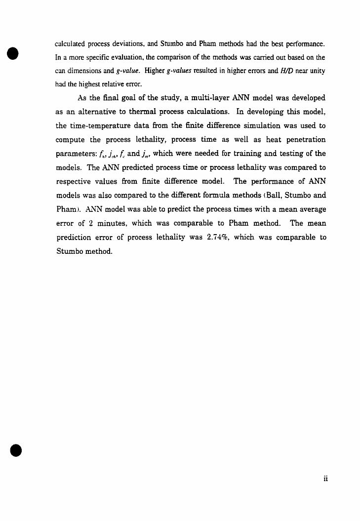
As the final goal of the studYt a multi-Iayer Al.~ model was developed
as an alternative ta thermal process calculations. In developing this model,
the time-temperature data from the finite difference simulation was used ta
compute the process lethality, process time as weIl as heat penetration
parameters: /:, i~fa' f.: and ier' which were needed for training and testing of the
models. The Ai~ preclicted process time or process lethality was compared ta
respective values from finite difference model. The performance of ANN
models \vas aIso compared ta the different formula methods (BalI, Stumbo and
Pham)...o\J.~~ model was able ta predict the process times with a mean average
error of 2 minutes, which was comparable to Pham method. The mean
prediction error of process lethality was 2.74%, which was comparable to
Stumbo method.
ii
•
•
RÉs~1É
L"applicabilité des réseaux d'intelligence artificielle (RIA) aux calculs impliqués
dans les traitements thermiques a été étudiée. Les travaux préliminaires consistaient à
développer des modèles RIA basés sur les données des méthodes de calcul du traitement de
BaIl et Stumbo. Le RIA basé sur la méthode de BalI tentait d~établir la relation entre la
t,'aleur-g• mesurant le temps de traitement.. et filU. mesurant le point d'asepsie du
traitement. L'optimisation de la taille des données d~entraînement du réseau" le nombre de
couches cachées, les noeuds dans chaques ces couches ainsi que les paramètres
d'apprentissage était cruciale pour l'obtention d'un modèle efficace. Pour le RIA basé sur
la méthode de Stumbo. le cheminement était similaire à celui utilisant la méthode de BaIL
mais celle-ci intégrait aussi la facteur de retardement du refroidissement.. jn:' Les modèles
RIA développés pour les méthodes Bali et Stumbo ont été validés en utilisant une série de
valeurs de g et f,/U obtenue en variant la température du milieu (TM)~ la température
initiale ITn. l'index de vitesse d'échauffement (/h). et les facteurs de retardement de
réchauffement (jch) et du refroidissement (jcc). L'erreur relative de prédiction était de 1%
pour la méthode basée sur 1" approche de Bail et 3% pour celle de Stumbo. La valeur
relativement élevée de 1'erreur pour la méthode RIA de Stumbo peut être attribuée au
nombre restreint de données d'tentrainement par rapport au nombre de paramètre. En
général.. les modèles RIA ont simulé de façon acceptable les méthodes de BalI et Stumbo
pour le calcul du traitement.
Pour mieux comprendre reffet des paramètres de traitement sur l'évaluation du
processus thennique't rexactitude de plusieurs formules (Steele & Board. BalI. Stumbo and
Pham) a été étudiée pour une variété de conditions industriellement utilisées. Une
simulation basée sur la méthode de différence finie à solution numérique du transfert de
chaleur dans un produit emballé dans un contenant cylindrique a été appliquée pour obtenir
les données de temps et de température reliées aux conditions d'étude sélectionnées (la
température du milieu. la température initiale.. diffusion thermique" taille de r emballage, et
longueur du traitement). De plus, la longueur de traitement et le point d~asepsie du
traitement ainsi prédits ont fait l'objet de comparaison pour évaluer ['effet de chaque
paramètre. La. température du milieu affectait de façon significative ['erreur sur la
iü
•
•
prédiction. Les méthodes de Stumbo et Pham ont produit les meilleurs résultats. Une étude
plus poussée démontre qu·une augmentation de la valeur-g entraîne une erreur plus élevée..
alors qu'un rapprochement du paramètre H/D.. relié à la dimension de remballage. à runité
se traduit par une erreur relative supérieure.
Pour but final de cette étude.. un modèle RIA rnulti--couches a été développé. Cette
alternative aux calculs du processus thennique. utilise les données de temps et de
températures obtenues par la simulation basée sur la méthode de différence tïoie pour
prédire I~ point d"asepsie du traitement, la longueur de traitement ainsi que les
paramètres de pénétrations de chaleurs: {,., j ..h1 t: and j~. Ces valeurs sont
nécessaires pour entraîner et tester les modèles. Les valeurs prédites par les
RIA ont été comparées aux valeurs obtenues par les calculs basés sur la
différence finie ainsi qutun nombre de formules acceptées (BalI, Stumbo and
Pham). Les modèles RIA développés ont pu prédire le temps de traitement
avec une erreur moyenne de 2 mins, une valeur comparable à celle obtenue
avec la méthode de Pham. L'erreur moyenne de prédiction pour le point d"asepsie
du traitement était de 2.74%, valeur comparable à l'approche Stumbo.
iv

•
•
ACKNO~DG&~NTS
l wouId like to extend my sincere appreciation and thanks to my thesis supervisor~
Dr. Hosahalli Ramaswamy for his guidance, valuable advice, encouragemenc keen interest
and support throughout the course of the study.
Also l aIse thank Dr. L Alli~ Chairman of the Departrnent of Food Science and
Agricultural Chernistrv and Dr. F.R.van de Voort for their mat advice at the stan of the..... ...study. ~lany thanks are also extended to Dr. S.O. Prasher. research committee member. for
his helpful suggestions on sorne aspects of the projece
r rhank Dr. S. Sreekanth for his very vaiuable help and advice in starting the projece
Dr...~Iain LeBail's rechnical assistance for modification of the flnite difference program of
Dr. S. Sablani (Ph.D. Thesis. 1995) for adoption to this work is gratefully acknowledged.
Nlany thanks to Dr. Farhad Salehi for his precious insight and guidance throughout the
study. .-\Iso. [ would Iike to thank ~ls. Aline Dimitri for the French translation of the
abstrJ,ct.
~ly sincere thanks to ail my colleagues in the Food Science Department. especially
the Food Processing group: Dr. Tatiana Koutchma. Dr. Reza Zareifard. Dr. Nlichelle
~[arcotte. Dr. Dina ~[ussa. Dr. Sasithorn Tajchakavit.. Nls. Sarmista Basale. ~Ir. PrJmod
Pandey. ~[s. Farideh Nourian. Mr. Harish Krishnamurthy. Mr. Curien Chen. ~Is. Lawrende
Chiu. ~lr. Olivier Turpin and ~Is. Nada Houjaij.
Above ail. 1 thank my wonderful parents. my dearest brothers. Keyhan and Soheyl
for their encouragement. love and suppon•
v
• a
D
t~
fhFu1:1e
h
hf
ITJœ
Jch
111
kt:
L
n
r
RT
T
te
T\,,",wtcr
e
T"eTo
U
E
XY
Yo
z
.:l
•
NOMENCLATURE
Significant dimension. the radius of cylinder (m)
Decimai reduction time (min)
Cooling rate index (min)
Heating rate index (min)
Process lethality (min)
Temperature difference between product and heating medium (reton) at end ofheating (IlC)
Vertical position in cylinder (m)
Fluid heut transfer coefficient (W/m!.K)
lnitial Temperature (oC)
Cooling lag factor
Heating lag factor
Bessel function of arder zero
Cylinder thermal diffusivity (W/m.K)
Lethal rate: Thickness or half thickness of a slab depending on il being heated orcooled from one side or bath sides. respectively
~umber of records
Radial position in cylinder (m)
Reton Temperarure (Ile)
Temperature (oC)
Time (min)
Cooling time (min)
Cooling water temperature (C)
Hearing rime (min)
Product temperarure at the end of heating (oC)
Reference temperature (oC)
Dimensionless temperature ratio =<.T-RT)/(IT-TR)
The equivalent of all lethal heut received by sorne designed point in the containerduring process at the reton temperature (min)
Distance from the coldest plane of a slab
.~'"N predicted valueDesired value
Temperature sensitivity indicator (CO)
Step size (used with space or time)
vi
• Subscripts
1.2 Refer to two levels with respect to temperature
Initial condition. space index
IT Initial condition of product
J Spaceindexref Reference
RT (Retort) heating medium
Greek symbols
a Thermal diffusivity (m~/s)
~ Roct of the characteristic equation (4.3)
.., Roct of characteristic equation (4.4)
Dimension Jess numbers
Bi Biot number
Fa Fourier number
AbbreviatioDs
•
Ai'INCERFI1R
LOS~[AE
~[ll\t[O
~lL\fN
~lRE
~
~~
OCR
PCA
PERMS
Artitïcial neural network
Carbon dioxide evolution rate
Fourier transform infrared
Linear discriminate analysis~[ean absolute error
~[ultiple input and multiple output~lulùple layer neural networkMean relative error
Near infra red
Nitrogen utilization rate
Oxygen consumption ratePrinciple component analysisProcessing element
Root mean square
vii

•
•
TABLE OF CONTENTS
ABSTRACT
RÉsc~lÉ iii
AC~'IOWLEDGMENTS v
NOME1\lCLATURE vi
LIST OF TABLES x
LIST OF FIGURES xii
CONNECTIN'G STAThvŒ1'ITS xiv
CONTRIBUTION OF AUTHORS xv
CHAPTER 1 L.'ITRODUCTION 1
CHAPTER 2 LITERATURE REVIEW 5
Principles of thermal processing 5
Kinetics of microbial destruction 6
Thermal process calculations 9
Thermal process calculation methocis [0
General method [0
Improved General method 11
Formula methods 12
Barrs method 12
Stumbo·s method 17
Hayakawa's method 17
Steele and Board's method 18
Pham's method 18
Evaluation of Formula methods 19
:'Iumericai models of thermal process calculations 21
Anitïcial neural networks 24
Development of an Al'lN modeI 26
Applications of ANN in Food Science and l\griculture 29
CHAPTER 3 ANN SIMlJLAnON OF HALL AND STUMBO FO~IULA
;\,IETHODS OF THERMAL PROCESS CALCULATIONS 3S
vii
ABSTRAeT 35• INTRODUCTION 36
Anificial neural network models 37
~[ATERIAL AND METHOOS 39
ANN modeling of BalI and Stumbo methods 39
Development of AJ.'JN models 39
BalI model 39
Stumbo model 41
Validating the ANN models 42
RESLLTS Al~1) DISCUSSION 43
ANN based BalI model 43
Nlodel development and oprimization 4-3
~[odel verification 4-9
AJ.~~ based Stumbo model 49
CONCLUSIONS 54
CHAPTER 4 COl\IPARISON OF FODIlTLA ~lETHODS OF THERl\-lAL
PROCESS CALCULATIONS FOR PACKAGED FOOOS IN
CYLINDRICAL CONTAINERS 55
ABSTR;\CT 55
INTRODUCTION 56
Brier review of formula methods 57Ball·s method 57Srumbo.5 method 58
Steele and Board's method 58
Pham's method 58~tATERIAL AND ~ŒTHODS 59
Finite difference program 59The basis of finite difference models 59
Overall accuracy evaluation of the fonnula methods 64-
Evaluation of fonnula methods under specifie conditions 65
RESULTS Al'ID DISCUSSIONS 65
Optimization of fmite difference model 65
OveraiI evaluation of formula methods 67
• Specifie evaluation of fonnula methods 73
viü
• CONCLUSIONS 79
•
CH..\PTER 5 ARTIFICIAL NEURAL NETWORK ~IODELS AS ALTERNATIVES
TO THE~IALPROCESS CALCULATION ~ŒTHODS 80
ABSTRACT 80
~TRODUCTION 81
~[ATER.L\L Al'fD ~ŒTHODS 82
Data generation 82
Al"~ model development 84
Optimization of Al'IN models 86
Comparison of ANN models with fonnula methods 87
RESCLTS AND DISCUSSION 87
~'IN models optimization 87
Performance of the Al'IN models 89
Comparison of A1~N models 92
CONCLUSIONS 99
CHAPTER 6 GENER.-\L CONCLUSIONS 100
REFERENCES 102
ix

• UST OF TABLES
Table 3.1 Combinations of training and testing data for network optimization 41
Table 3.! Range of network architecture and learning parameters used in thestudy 41
Table 3.3 Range of parameters for validating k\fN based BalI and Stumbomodels 43
Table 3A Effeet of PEs and hidden layer(s) on the performance of .-\1'fNbased BalI models 46
Table 3.5 Effeet of epoch size on prediction ability: AJ.'lN based BalI models 46
Table 3.6 Effect of momentum on prediction ability of AJ.'m based BaliModels 47
Table 3.7 Optimallevels of architectural parameters for .-\l~~ based Bali andStumbo models 47
Table 3.8 Error parameters for AZ~"N based BalI and Stumbo models 49
Table 4.1 Errors in process rime calculation influenced by processingconditions and thennal diffusivity of product 69
Table 4.2 Errors in process lethality calculation intluenced by processingconditions and thennal diffusivity of product 69
Table -t3 ~Ieans and Standard Deviations (SD) of relative errors in processtime caIculations for selected process calculation methods 71
Table -l.A ~leans and Standard Deviations (SD) of relative crrors in process[ethality calculations for selected process calculation methods 72
Table 4.5 Maximum. Nlinimum. ~[ean and Standard Deviations of errors fordifferen t methods 72
Table 5.1 Range of parameters used in finite difference program 83
Table 5.2 Combinations of training and testing data for network optimization 86
Table 5.3 Range of network architecture and Iearning parameters used in thestudy 87
• Table 5A Effect of momentum. and epoch size on the perfonnance of ModelAandB 89

Table 5.5 Error parameters for perfonnance and verification of Al~'N models• AandB 92
Table 5.6 ~[eans and Standard Deviations (SO) of relative errors in processtime calculations for selected process calculation methods 95
Table 5.7 ~[eans and Standard Deviations (SD) of relative errors in processlethality calculations for selected process calculation methods 96
Table 5.8 Range. mean and standard deviation of errors for aIl thecombination of parameters 96
•
• UST OF FIGURES
Figure 2.1 Typical semi logarithmie heating and cooling curves 13
Figure 2.1 Grid format for temperature calculation using a numerieal method 23
Figure :!.3 Basic structure of a biologicaJ neuran 25
Figure lA Typieal diagram of Al'lN model 25
Figure .!.5 Diagram of a processing element and related calculations 27
Figure 3.1 Learning curve for ANN model A (prediction log g) .f5
Figure 3.1 Learning curve for ANN model B (prediction f,/U) 45
Figure 3.3 Comparison of .-\l'IN predicted vaIues and Bali table parametersrespect ta input variable 4-8
Figure 3A Validation of ...u'IN models of BalI method 50
Figure 3.5 Comparison of A.N'N predicted values and Stumbo table parametersrespect to input variable 52
Figure 3.6 Validation of AN~ models of Srumbo's method 53
Figure .f.l Optimization of tïnite difference model for al number of nodes ineach a:<is and b) time step 66
Figure ·tl Validation of tïnite difference model against the analvtical solution 68~ -
Figure .f.3 Errors in process time caIculations for different g-vaIues (a: g=O.05C. b: 2=1 CO: c: g=5 Co: d: 2:=10 CO: e: 2=15 CO) 74- . ~ ~
Figure .fA Errors in process lethality calculations for different g-values (a:g=O.OS CO. b: g=l CO; c: g=5 C: d: g=IO CO: e: g=IS c; 75
Figure -t-.5 Errors for process IethaIity calculations with respect to different g-values (a: Steele & Board's methocL b: Ball's method; c: Stumbo'smethod) 77
Figure ..t6 Errors for process time calcuIations with respect to different g-values (a: Steele & Boarcrs metho<L b: Bairs method: c: Smmbo'smethod: d: Pham's method) 78
• Figure 5.1 Arrangement and procedure of developing AJ.'lN models 85
xii
Figure 5.2 Learning curve for ANN model A 88• Figure 5.3 Learning curve for Al'fN modeI B 88
Figure 5A- Effect of PEs and hidden layers on the performance of model AandB 90
Figure 5.5 Performance of AJ.'lN models A and B with respect to predictedoutput 91
Figure 5.6 Performance of A1';~ models A and B in process time and processlethality prediction 93
Figure 5.7 Performance of Ai'1N model in process time calculation incomparison with the other selected Formula methods 97
Figure 5.S Performance of A:.'lN model in process lethality calculation incomparison with the other selected Formula methods 98
•XÏü

•
•
CONNECTING STATEl\'1EJ.'ITS
This thesis research is divided into three parts. The first pan is a feasibility study
demonstrating the potential of ANN modeling in simulating two simple (and most popular)
process ca1culation methods (BalI and Stumbo methods). In this pan.. input for the Al'IN
models were obtained from tables developed by Bail and Stumbo. which large1y simplifies
the situation for generating input data. The development of such simplified AJ.\fN models is
described in Chapter 3. and tS part of the manuscript number 4 listed on next page.
The accuracy of existing fonnula methods against the data predicted by a fioite difference
computer model under a range of commercial operating conditions were evaluated in the
next chapter as a prelude ta developing a more general Al'IN model. which is the final
objective of the study. This aspect is detailed in Chapter -+ demonstrating the discrepancy
of sorne process calculation methods in predicting accurate values under certain
circumstances. This forros the basis for another publication (number St
The tinal Chapter 5 i5 the principal fceus of this srudy. However. the basis for the
developed final ~~'N models came from Chapter 3 (for optimizing the fu~N performance)
and Chapter -+ (. for generating the input data using the finite difference mode[). The
different methods are ultimarely compared in Chapter 5. demonstrating the utility of A1\fN
models. This aspect fonns the basis of the final manuscript (number 6). The details of the
manuscripts/presentations arising From the thesis are highlighted in the next section with an
explanation to the raIe of co-authors.
xiv
•
•
CONTRIBUTION OF AL'THORS
The following papers have been prepared for different presentations and/or publications:
1. Afaghi. ~1. and Ramaswarny. R.S. 1997. A neural network approach for thermalprocess ca1cularions. Presented at rhe CIFST AnnuaI Conference. Radisson Hotel.~[ontreal. QC. September 22-25.
2. Afaghi. ~[ and Ramaswamy. R.S. 1999. Artiticial neural network models asalternatives to formula methods of thennal process calculations. Presenred at theCIFST AnnuaI Conference. Grand Okanagan Horel. Kelowna. BC. June 6-9.
3. Afaghi. NI. and Ramaswamy. H.S. 1999. Comparison of formula methods of thermalprocess calculations for foocis in cylindrical containers. Presented at the Annual~{eeting of the [nstirute of Food Technologists (IFT). ~[CCormick Place South.Chicago. IL USA. July 24-28.
-1.. Afaghi. yI. and Ramaswamy. H.S. 1999. A1\fN simulation of Bail and Srumbo formulamethods of thermal process calculations. (Submitted. Food Research International).
5. Afaghi. ~l. and Ramaswamy. H.S. 1999. Comparison of formula methods of thermalprocess calculations for cylindrical packaged foods. 1To be submittedt
6. Afaghi. yI. Ramaswamy. H.S. 1999. Artificial neural network models as alternative ofthermal process calculation methods. <To be submitted)
[n the above papers. ail the experimental (modeling) work. analysis of results and
preparation of manuscripts were done by the candidate (~1. Afaghi). under the supervision
of Dr. H.S. Ramaswamy.
xv

•
•
CHAPTERI
LNTRODUCTION
Thermal processing is one of the most imponant methods of food preservation of
the twenrierh century. Since the innovation of this method by Nicholos Appert in i810.
thennal processing of packaged fooels has been improved extensively in ail related aspects
of the process. Design of an effective process requires a sound knowledge of the
destruction kinetics of the concemed microorganism and temperarure history of the
product. Process calculation rnethods are commonly designed to compute the required
processing time for a target sterilization value or to ~valuate the sterilization value for a
given process. Accurate process caIculation methods are required with respect to bath
safety and quaIity consideration of product.
Bigelow et al. (1920) established the first graphical procedure of thermal process
determination. referred as General method. Bali (1923) introduced a mathematical method.
known as the tïrst Formula method. Bail's method has broadly served the food industry
despite sorne of its sweeping assumptions. which results in sorne inaccuracies. BalI' s
fonnula method is based on the equation for the straight-line portion of tlie semi
logarithmic hearing curve at the cao center. Ta calculate the process time for defined
process lethality or to calculate the lethality of a given process. Bali developed sorne tables
and graphs. Srumbo' s method ( 1966). developed as the revised version of Bali' s method.
result~ in more accurate process calculations (Smith and Tung. 198:2). However. the
procedures of process calculation in these two methods are quite sirnilar and the accuracy
of each rnethod depends on the accuracy of the evaluated parameters and addition of
correct cooling lethality to process calculation through the tables and graphs. The
application of these tables and graphs can be time consuming and may become a source of
error in process calculations. In addition ta these [wo methods.. several other methods e:dst
in literarure as alternatives to the existing process calculation methods developed through
modifying procedures (Hayakawa. 1970: Pham. 1987. 1990: Vinters. 1975: Steele and
Board. 19ï9a.b).
•
•
Smith and Tung (982) evaluated the accuracy of sorne fonnula methods as
compared to a numericaI method for a range of processing conditions and can sizes. and
poinœd out differences in their performances. Studies have been aIsa carried out [0 check
the accuracy of fannula methods in relation to a computer simulation of thermal processing
using finite difference numericaI solutions for thin profile packaged foods tGhazala el aL.
(990). Stoforos el aL (1997) reviewed in detail the basis of different methods of process
calculations and the accuracy of these methods as compared to a tinite difference
simulation of heut transfer for one set of processing conditions and can size.
Advent of computers and ease of programming has provided the potentia!
application of mathematical roodels in process design.. validation. controL and optimization
(Hayakawa. 1970. 1978: ~lanson et al.. 1970: Stumbo. 1973: Teixeira et aL. 1969a. b:
Teixeira.. 1978). These models are mainly used in temperature protile prediction of product
undergoing thermal processes. as they provide a more versatile alternative to rime
consummg and expensive heat penetration tests. [n addition to time-temperarure
prediction. with these roodels the retort temperarure need not be held constant and cao be
vmed in any prescribed manner throughout the process. The rapid evaluation of an
unscheduled process deviation is another important application of these models tHeldman
and Lund. (992).
The application of anitïcial neural network t.fu~') methods has been growing in
the several :ueas of food technology and agriculture. fu'IN is a powerfUl technique for
correlating data using a number of processing elements. Lsing the .-\.'fN technique. the
computer leams to make intelligent decisions using known input-output data and adjusting
sorne internal parameters of the network through repetitive introduction of known
examples. The strength of ANNs is in their ability to handle complex nonlinear
relationships with ease and without any prior knowledge of their relationships. The Al'IN
has polentia! advantages of adaptation and learning ability. fault tolerance of noisy or
incomplete data. and high computationaI speed. Eerikainen et al. (1993) introduced the
early application of neural networks in food related subjects. .~'lN has shown a promising
application in extrusion process control (Eerikainen et al.. 1994), As an alternative ta
statistical models in data analysis of FfIR. GS-MS and sensory evaluation. AJ.'\iN models
had a higher performance (Bochereau et al.~ 1992: Tomlins and Gay. 1994: Vallejo-
2
•
•
Cordoba et al.. 1995). Sablani et al. (1995) investigated the potentiai of A1'lN models for
prediction of optimal sterilization temperatures.
One typical type of Ai.'lN structure in known as back-propagation networks. which
has shown promising results in prediction modeling and classification (Sreekanth el aL.,
1998~ Lacroix. et al.. 1997: Bochereau et al., 1992: Freeman. 1993). A back-propagation
network consists of a sequence of layers with full connection between the layers. Three
required layers in these networks are input layer.. hidden layer(s) and output layer. Input
layer transfers the input information to the network to be processed by hidden layer(s). The
processed information is passed to an external source through the output layer. During
training. the internai parameters are adjusted to produce the possible c10sest k\fN output ta
the desired output. The adequacy of a trained network depends on the nature and size of
the training data set as well as selecting the optimal internaI parameters. In other words.
the performance of the ANN model greatly depends on the training data with respect ta
bath quantity and quality (Swingler. 1996). Once trained. the AJ.\fN model presents rapid
answers to any input variable in the domain of training data sel. If the conditions change in
such a way that deprives perfonnance of the network. the Al.'IN model can be trained
further under the new conditions ta correct its performance (Baughman and Liu. (995).
Considering th~se abilities. AJ.'iN models render themselves as a possible alternative ta
mathematicaI models and regression techniques (Ni and Gunasekaran. 1998~ Tomilins and
Gay. 1994),
During the sterilization process. there are severa! parameters. which affect the
accuracy and efficiency of heating process evaIuation. The most relevant factors in
evaluation of a heat treatrnent are type and heat resistance of microorganisms. pH of food
product. heating conditions. thenno-physical properties of food and package size and type
1Valenras et al.. (991). An accurate thennaI process caIculation model takes into account
the signitïcance of producing a high quality product while ensuring the minimum required
qualiry.
The following were the objectives of this research:
3

• 1.
1
3.
Development of A1'\lN models based on input data from Bali and Stumbo's tables as
J. preliminary study to evaluate the feasibility of ANN models in thermal process
calculations~
Evaluating the accuracy of different formula methods over a wide range of
processing condiùons and can sizes against a reference computer simulaüon model
based on numerical solution of partial differential equations related to heur
conduction equa[ion involving finite cylinders.
Development of an M'lN model using the data obtained from the finite difference
simulation under a wide range of conditions and comparison of the performance of
A.\j~ model with traditional fonnula methods.
•
Successful thermal processing encompasses the assurance of safety and high quality
ùf the food products. Several methods developed to establish thermal processes have been
improved with respect to innovation and application of computers in food technology. [n
this study. ~rtitïcial neural network technique is being evaluated [0 develop a possible more
versatile thermal process calculation method. Due ta the fact that A~'N technique has the
ability in modeling non-linear systems. it is hoped that ~'IN based thermal process
calculation model will he capable of pursuing me objectives of an nccurate thermal process
caiculatÎon model.
4

•
•
CHAPTER2
LITERATURE REVIEW
Principles of thermal processing
Thermal pracessing of packaged foocis basically involves heating of food products
for a selected rime at a selected temperature ta destroy pachagenic microorganisms
endangering public health as weil as thase microorganisms and enzymes that deteriarate
the food during storage. For the first time. Nicolas Appen. in 1810. introduced the concept
of in-container thennal processes. Extensive emphasis has been given ta improvements in
thermal processing. as this is one of the mosr important methods of food preservation.
Although the heur labile nature of microorganisms is the basis of thennally preservation of
food products. yet the same but undesirable effect can destroy part of nutrients and quality
factors. Therefore. an efficient thermal processing requires to be accurarely designed to
ensure bath the safery and quality of food products.
An effective thermal processing is defined based on the detïnition of commercial
sterilization. Commercial sterilization of food producr inhibits the growth of both
microorganisms and their spores under normaI storage conditions in the container. A
commerciaJly sterile food product may contain viable spores. such as thennophilic spores.
which will not develop under normal storage conditions. The US Food and Drug
Administr.ltion in 1977 defined the concept of ftminimal thermal process" as "the
application of heat to food. either before or after sealing in a hermetically seaIed container.
for a period of rime and at a temperature.. scientifically detennined to be adequate ro ensure
the destruction of microorganisms of public health concem."
Severa! important factors determine the extent of thermal processing. such as:
1) Type and heat resistance of the target microorganism.. spore or enzyme
2) pH of food product
3) Heating conditions
-1-) ThermophysicaI properties of food product and container shape and size
5) Storage conditions following the process
5

•
•
The primary step in thennal process establishment. which is defining and selecting
the target microorganism or enzyme~ is directly related to food product conditions.
Temperature and oxygen are important factors in optimum growth of microorganisms.
Based on appropriate remperature for growth, microorganisms are c1assitied into
psychrophiles with rapid growth between 0-5°C, mesophiles with optimum growth between
5~OL.lC and thermophiles with optimum growth at temperatures higher than 40LlC (Rose,
1965). With respect to oxygen requirement for growth. microorganisms are classified as
obligate aerobes'O facultative anaerobes and obligate anaerabes. Packaged foods under
vacuum in sealed containers provide low levels of oxygen. therefore. these conditions do
not support the growth of obligate aerobes.. and further the spores of obligate aerabes are
(~ss hear resistant to heat as compared to the spores of facultative and obligate anaerobes.
The growth and activity of anaerobic microorganisms are highly pH dependent. From a
thermal processing standpoint'O foods are divided into three graups based on pH:
1) High acid foods (pH<3.7)
2) Acid or medium acid foods (3.7<pH<4.5)
3) Low acid foocis (pH>4.5)
[n thennaI processing a special attention is devoted ta CLostridùlIn botulinum which
is a highly heat-resistant.. spore-forming.. anaerobic pathogen that produces botulism toxin.
Clostridill1ll botulinum does not generaIly grow and produce toxin at pH below 4.6.
Therefore.. in thennaI processing. a. pH of 4.5 is considered as dividing line between the
acid and low acid food products. Molds. yeasts and bacteria. which tolerate high acidic
conditions are targeted in thermal processing of high-acid food praducts. Bacillus
coagulase and Saccharomyces cerevisiae are important in high-acid foods.
~licroorganisms such as Bacillus Stearothermphilus'O Bacillus thermoacidurans and
Clostridium thermodaccolyticum are more heat resistant than C. bontlinum. but they are
mostly thennophilic in nature and in case of storage of cans at temperatures below 30°C..
they are not of much concem.
Kinetics of microbial destruction
EvaIuating the thermal resistance of target microorganisms is required in thermal
processing design. Thermal destruction of microorganisrns generally fol1ows a first-order
6
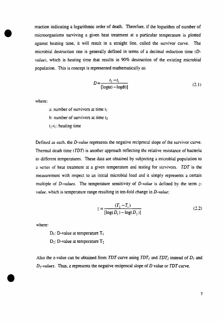
• reaction indicating a logarithmic order of death. Therefore. if the Iogarithm of number of
microorganisms surviving a given heat treatment at a partÏCular temperature is plotted
a!!ainst heating tirne. it will result in a straieht line. called the survivor curve. The'-' .... .....
microbiai destruction rate is generally detïned in terms of a decimal reduction time (D-
value), which is heating time that results in 90% destruction of the existing microbial
population. This is concept is represenred rnathematically as:
where:
D[logtl) -log(b)]
a: number of survivors at time [t
b: number of survivors at rime t1
[:-[1: heating rime
(2.1 )
Detïn~d as such.. the D-value represents the negative reciprocal slope of the survivor curve.
Thennal death time (TDn is another approach reflecting the relative resistance of bacteria
to different remperatures. These data are obtained by subjecting a micrabial population to
a series of hear treatment at a given temperature and testing for survivors. TDT is the
measurement with respect to an initial microbial laad and it simply represents a certain
multiple of D-vaLues. The temperature sensitivity of D-value is detïned by the term :
ralue. which is temperature range resulting in ten-fold change in D-value:
where:
... -[log(Dt ) -log(Dz)J
D,: D-value at temperature T,
D~: D-value at temperature Tz
(2.2)
•AIso the z-value cao be obrained from IDTcurve using TDT[ and TDTz instead of Dl and
Dl-values. Thus. z represents the negative reciprocaI sIope of D value or TDTcurve.
7

• In order to compare the relative sterilization capacities of thermal processes~ the
terro lethality (F-value) is introduced. The F-value is detïned as the nurnber of minutes
required at a specifie temperature to destroy a specitied number of microorganisms with a
specifie :-vaLue. For convenience a unit of Iethality is detined as equivalent hearing of one
minute at a reference temperature of 121oC (250~ for the steriliza[Îon process. Thus. the
F-vallie represents a certain multiple or fraction of D-value depending on the type of
microorganism. ~Iathematicai equivalent of this definition is:
where:
'T,-Tl
F=nD=F.lO ="
T" Reference temperature
E,: Lethality at Tt)
(1.3)
Lethal rate is defined for comparing different processes in terms of achieved lethality and it
is considered to be the heating time at the reference temperature relative to an equivalent
heating of one minute at the given temperature:
T-Trr;
L=LO : (2.4)
[n a real process in which the food product undergoes a time-ternperamre protïle. the lethal
rate is integrated over the processing rime to result in an ovenul process lethality (also
defined by F,.):
t
Fil =fL.dtrj
(2.5)
•[u terms of food product safeey. assurance of a minimum lethality at the thermal center of
food product is required. However it is desirable ta minimize the overall destruction of
quality factors.
8

• Thermal process calculations
The purpose of thermal process calculations is to determine an appropriate process
time under specified heating conditions required ta achieve a given process lethality or
~stirnating the lethality for a given process. Thermal process deterrnination through a
physical-mathematical approach requires the basic information of thermal destruction
kinetics of microorganisms and quality factors conjoined with time-temperature data of
product to integrate the lethal effects of thermal processing.
Therefore. an efficient process design requires sound information on the heat
penetration data and their characteristics. Heat penetration data. are function of severa!
factors and different combinations of factors can result in same process lethality. These
factors can he summarized as follows:
1) ~[ethod of heating process (eg. still process vs. agitated process)
2) Type of heating medium (steam. water)
3) Heating conditions (reton ternperature. initial temperature of productl
4) Product type (solid. liquid. particu[ate)
5) Container type. shape and size
Obtaining accurate data regarding the heating and/or cooling of a food product in
container is important for accurate detennination of time and temperature with respect to
sterilization of a given product. However.. it is impractical to obtain hear penetration
protïles for the whole range of conditions. Accordingly.. thermal process calculation
procedures are developed with ability of time-temperature prediction with respect to sorne
experimentally deterrnined parameters. Obviously. the applicability and restrictions of each
method are defined by the assumptions taken inta account to obtain temperature prediction
mode1.
Following each heating phase of thermal processing operation is a cooling phase to
control and terminate the lethal effect of thermal processing. In order to account the
cooling effect. the lethality equation (2.5) can he rearranged as folIow:
•, :
F = J- 10 •T - T~ I!:: dt"
o
t.
+ J10 1T - T~ 1::: deo
(2.6)
9
•
•
where:
tg: total heating time
dt: small time interval
le: total cooling time
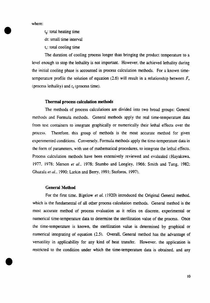
The duration of cooling process longer than bringing the product temperature to a
level enough to stop the lethality is not important. However. the achieved lethality during
the initial cooling phase is accounted in process calculation methods. For a known time
temperature profile the solution of equation (2.6) will result in a relationship between Fr,
(process lethality) and Cr: (process time).
Thermal process calculatioD methods
The methods of process calculations are divided into two broad groups: General
methods and Formula methods. General methods apply the real time-temperamre data
l'rom test containers to integrate graphically or numerically their lethal effects over the
process. Therefore. this group of methods IS the most accurate rnethod for given
experimented conditions. Conversely. Formula methods apply the time-temperature data in
the forro of parameters. with use of mathematical procedures. to integrate the lethaI effects.
Process calculation methods have been extensively reviewed and evaluated (Hayakawa.
1977. 1978: ~[erson et al.. 1978: Stumbo and Langley.. 1966: Smith and Tung. 1982:
Ghazala et al.. 1990: Larkin and Berry. 1991: Stoforos. (997).
GeneraI ~(ethod
For the first time. Bigelow et al. (1920) introduced the Original General method.
which is the fundamental of ail other process calculation methods. General method is the
most accurate method of process evaluation as it relies on discrete. experimentaI or
numerical time-temperature data to determine the sterilization value of the process. Once
the [Îrne-temperature is known. the sterilization value is derermined by graphical or
numerical integrating of equation (2.5). OveralI.. Generai method has the advantage of
versatility in applicabiliry for any kind of heat transfer. However. the application Îs
resrricted to the condition under which the time-temperature data is obtained. and any
10
• change in either processing conditions (retort temperature. initial temperature)~ product or
package size requires a related temperature profile.
The original General method is based on lethal rate as the reciprocal of TDT value.
The area under the lethal rate curve vs. heating time will result in a sterilization value of the
thermal process. In arder to detennine the process sterilization value (Fil) \Vith General
rnethod. different works has been carried out, both in graphical and numerical Integration
to make chis method less [aborious. Schultz and Oison (1940) developed lethaI rate papers
and dimensionless temperature differences in faons of TRrTffRrTrr to account for
variation in reton temperature and initial temperature of product independent of
experimenrally obtained data. E;(tended works have been carried out for different z-values
and procc:ssing temperatures (Cass.. 1947: Hayakawa. [973: Leonhardt. 1978). Simpson's
mie. [rapezoidal mie and Gaussian Integration are improved techniques for numerical
imegration. Patashink l L953) used a trapezoidal mie by considering sorne assumptions in
this tt:chnique. Hayakawa (1968) developed a method using Gaussian Integration fonnula.
involving a remplace, which couId be used with the graphical method.
The limitation of General method is in determining the process lime for rarger
process lethality. For this purpose a trial and error method is proposed. Also it is tedious
ta consider a leth'al rate curve during cooling which depends on the heating rime. Often a
singlt: shape of cooling curve is imposed irrespective of the heating curve. Obviously. this
cannat be right for aIl situations as the lethal rate is related to temperarure difference of the
product and heating medium at the end of heating (g-va[lle) and this assumption applies to
onl y to cases with g-value close ta zero.
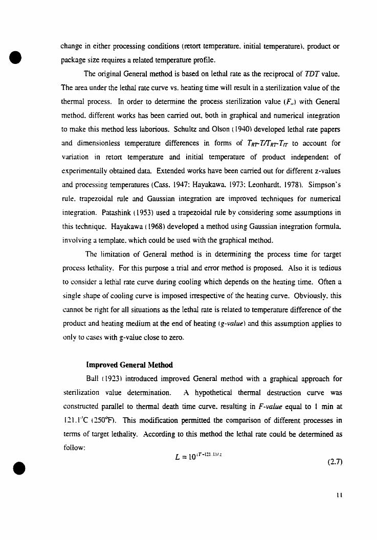
Improved General ~(ethod
BaIl (1913) introduced improved General method with a graphical approach for
sterilization value determination. A hypothetical thermal destruction curve was
constructed parallel ta thennal death time curve. resulting in F-value equal to 1 min at
1:!1.1 ·Je (250~. This modification permined the comparison of different processes in
terms of target lethality. According to this method the Iethal rate could he determined as
follow:
•L =lO,r-l!l.ll/:
(2.7)
il

•
•
The area under the curve. resulting from ploning L vs. heating time. represents the
equivalent minutes at 121.I lle. The urea under the curve can be determined by counting
the number of squares. using a planimeter or by approximating to standard shapes. AIso
for this method. process time determination for target process lethality requires a trial and
error technique.
Formula ~Iethods
The procedure that Bali (1923) applied in thermal process calculation was the basis
for a new set of methods termed ··Formula. methods·... Process determination using Fonnula
methods is considerably faster due to applying heat penetration data in form of heating and
cooling rate indexes (fil andJ~) and lag factors (jc:h andjtr). Formula method determines the
process rime for a pre-selected process lethality or alternatively. process lethality of a given
process. H~nce using the parametric fonn of heut penetration data with appropriate
mathematical procedures. the effect of processing conditions (Jeton temperature and initial
temper~ture of the product> as weil as the effect of different package sizes. Following is a
brief review of sorne of the most applied Formula methods.
Ball's method: As mentioned previously. Balrs method (1923) is considered to be
the tïrsl developed Formula method and it has a great contribution to the value of
mathematics in food processing (Merson et al.. 1978). BalI developed equations for
predicting the temperature al the critical point inside a cano This equation was applied in
general equation of (2.5) to determine the process lethality. The temperature prediction
equations were based on the experimental observations that a semilogarithmic plot of the
difference between medium and product temperatures vs. rime. after sorne initialtime lag.
was usually a straight line. The same approach is applied for cooling portion. 5uch typical
heating and cooling curves are shown in Figure 2.1. They basically comprise of a
hyperbolic heating lag portion. a logarithmic straight-line heatingy a hyperbolic cooling lag
and a logarithmic straight Hne cooling. BalI ignored the effect heating lag portion. as in
usual conditions the product temperature in below the Iethal temperature and the
accumulated achieved lethality is negligibie. However. the effect of heating lag can he
included for processes with high fI,. large :-value. or processes with low heating required
12

80
•
Heating Curve
100 _. 1
--...._---,_.
~ ~'
: IO:~='~-~==:=='='=-='~-,~~ __'8 ~:=:__.._.. ~~~§~L;~~~~tt :=---~=::_;.....---..-..---.- ..----
- ...--- --..-..-,------t~ ------- ------_._-----
T '--__........LI ....I ...lI~__._I
Q 20 olO 60
Tme (rnn)
Cooling Curve
'000
cr~
ê'S- taO ~jeu~ -...CI ,.S; -~
~.........
tO ' .......
g i---
'8 -_.~
ttt 1 1 1 1 1
a 20 .lO 60 80 TaO t20
Trre (rm)
•
Figure 1.1 Typical semi-Iogarithmic heating and cooling curves
[3

•lethality. Foh• Therefore. only the equation for the straight-line portion was considered for
the heating portion. This equation with respect of heating rate index (fi.) and heating lag
factor (jh) was described as follows:
where:
T =T - J' (T - T )lO-r,,:' l"RT <:h RT IT
TRT: retort temperature (oq
T rr: initial temperature of the product (oC)
th: hearing rime (min)
fh: heating rate index (min)
jl.:h: heating lag factor
(2.8)
For the cooling curve. the effect of cooling lag \Vas considered in calculation of
sterilization vaIue. After start of cooling. the crilicaI center of the package is still al lethai
temperatures and the effect of this lag should be considered in addition ta the logarithmic
straight portion of the cooling. In order to account for cooling. BalI used two separate
equations to predict the temperature during cooling.
For the tÏrst portion or when 0 ~ t..- ~ 1.. log( j, 10.657 ):
The temperature in the criticai point of the package was predicted with Equation
•
r J: \: l
T = T~ ~ 0.31 T. - T ) x [- 1~ [ t :. ..... _ 0.5275 loge l 10.657 ) f) J
where:
~: cooling rime
jl:: cooling Iag factor
f~: cooling rate index
Tg: product temperature at the end of heating
(:2.9)
14

•T~: cooling medium temperature
For the straight-line portion of the cooling curve when the equaùon was same as
heating ponion with reIated coaling f c: log( j L- 10 .657 ) ~ t.:
T = T + J. (T - T )10 - t. { 1.cw c: ~ cw (1.10)
•
After defining the temperature prediction equations. BaIl substituted (hem in the
equation (2.5). The resulting equation cauld nat he integrated analytically and concluded
in a direct relation between Fil and tg lprocess ùme). Hence Bail solved the equation
graphically by evaluating the resulting integraIs. The results of integrals were presented in
table and graph fonnats. These tables and graphs related g-value. as a measure of process
time. to Ji/LI ratio. as a measure of sterilization value. BalI applied parameter U as the F
value of the process at the reton temperature. These tables and graphs could be applied for
uny:-vafue.
During development of the tables and graphs. BalI assumed a constant cooling lag
factor (j. 1). equal to 1A 1. Aiso the heating rate (/h) was applied for the cooling portion. or
in other words t... was equal to th. Further. in the development of the methad (Bali and
Oison. [95ï). with respect to two dimensionless parameters of Ph and P,: for determining
the sterilization value. they accounted for variation offh andi. Obviously the conditions of
aH processes do not comply with these assumptions and result in eITors in process
calculations. ~Ierson et aL (1978) and Hayakawa l(978) evaluated this method and
reported the inaccuracies of the method. BalI method overestimates the process lime.
which provides a safety factor (Merson et aL. 1978) for process calculations.
The time duration until retort reaches the processing cemperature is termed come-up
rime 1CCT) and a ponion of this cime can hold lethality effect. BalI assurned 42% of chis
time should be added ta process time. which hoIds the product at retart temperature uotil
the steam off. He implemented chis time duratioo in his method by shifting the zero of the
heating time axis by 0.58 of eUT. It should be mentioned that this percentage is not
aIways same and severa! researchers have caken into accoUDt to carefully evaluate the
effect of CeT (Hayakawa and Bail. 1971: Ramaswamy~ (993).
15
•
•
Further there are sorne food products that do not follow a constant mode of hear
transfer. and due to modification of the nature of the food product during the heating, the
mode of heat transfer will change. This condition of heatine is known as broken heating~ - -
and is more common of those kinds of food products initially heat by convection: then. due
to the activity of sorne thickening agents as starch gelatinization, the mode of heat transfer
changes to conduction. Bali and Oison (1957) accounted for this effect by considering two
straight-line segment of the heating curve with different slopes instead of one straight line
(broken heating) in semi-logarithmic hearing graph.
Hicks (1958) round severa! marhematical errors related [0 the lethality of heating
phases. F"h' in BalI and Olson's parametric values. He prepared a numerica.! table of
recalculated parametric values. Gillespy (1951) defined a method for estimating the F
\"ldut! for the whole can by using Balrs asymptotic approximation for heating and
developed an approximate method for cooling. Hemdon et al. (1968) prepared compurer
denved tables based on Ball"s method. Griffin el al. (1969: (971) improved these tables for
broken-heating curves and for cooling curves. Pflug (1968) compiled abridged tables from
BalI and Olsoo's tables and aIso from Hick's table in parametric values and considerably
simplitïed [he caIculation required for process evaluations.
Spinak and Wiley ( (982) reviewed BaII"s method and considered the accuracy of
method in comparison with a General method. [n this work they compared the process
rimes for processing selected food products in retart pouch with respect to Bail"s method
assumptions and reaI vaIues from the process. The result shawed the process time
detennined by BalI"s fonnula method requires the effect of reton come-up time lethality
and the actual cooling lag factor UnJ. However. actual j~. value showed no significant
effect in at:curacy of Bali's fonnula method.
In a funher review of Ball's method (Steele and Board. 1979a). the inaccuracy of
BaIl"s method was considered to he in a safe region for underestimating the process
sterilization ratio. Therefore. it was concluded in this work that related inaccuracy
introduces a safety factor to sorne calculated processes and of course me producüon of safe
products is one of the prirnary criteria of thermal processing.
16
•
•
Vinters et al. (1975) parameterized the data from the tables in Balrs formula
method. replaced tables and graphs in this method by algebraic. regression equations.
Therefore. this method could be used in a programmable calculator.
Stumbo's method: While attempting to revise the tables developed by Bail.
Stumbo and Langley t1966) developed a new set tables ta account for the variability of jo:
values. The values of these tables were abtained by graphicai measurement of hand drawn
temperurure profiles plaued on the lechal rate papers and subsequent interpolation of these
tables. As the authors implied. these tables were applicable for cases in which the
difference between fh and (were less than 20% of the respectivefh values.
Larer. the revised form of these tables were published (Stumbo. 1973t The revised
tables were based on computer integration of temperature protïles generated from heat
tr~nsfer equarions.. using tïnite difference simulations. However. it should be noted that
these tables are applicable aoly whenJirJ~· (Hayakawa.. (978). A correction for Jh~i· can be
made as long as the value for the heating lethality cao be obtained through a different
method 1Stoforos.. 1997). The rest of procedures for process calculation were same as
Bail"s method. Computer irnplementatÎon of Srumbo's method was introduced first by
~[anson and Zahradnik ( 1967). using Stumbo and Longley's tables and after by Tung and
Garland 11978 t using Stumbo's revised table values.
Hayakawa's method: For the tïrst time Hayakawa (1970) applied a set of
empirical formulas. each of them eoncerned to a specifie range of j values. The curvilinear
parts of the heating and cooling eurve were represented by exponential cotangent and
cosine functions. The minimum and ma:<imum j values that are related to these tables are
0.045 and 3.0. respectively. He also prepared a table of new parametric values by using his
empiricaI formulas .. and developed a procedure for the evaluation of heat processes. These
tables were applicable ta aImost any :-value.. resulted in eliminating the required
interpolation for the =-\'alue. Therefore.. the process calculation was significantly
simplitïed.
li

•
•
Steele and Board's metbod: Steele and Board (l979b) and Steele et al. (1979)
reviewed Ball's method and improved this method by introducing sterilization ratios to he
used instead of temperature differences. This ratio was defined as the temperature
difference between the heating (or cooling) medium and product by the slope of the
thermal death time curve for the concerned microorganism. C'sing these dimensionless
ratios \Vas advantageous in four main aspects. Firstly. the method could be applied for any
tempertlture scale whilst the same scale was used in determining the sterilization ratios.
Secondly. the number of associated tables were less compare to Bail·s method as z-value
was incorporated in the sterilization ratio. Thirdly. the tables could be approxirnated more
readily for a programmable calculator. as one variable was eliminated and tïnally. the
limits of integration were selected in such a way that errors in tabulated values were
negligible.
Pham's method: In an attempt ta revise and improve the Stumbo's method. Pham
( 1987) introduced two serious of algebraic equations for thermal process calculation. The
method relied on the conduction heat transfer equation of a tïnite cylinder. Heat transfer
coefticient at the container walls was intinite and the initial temperature distribution was
uniform. Two ranges of sterilization values were considered: high sterilization value or in
cases when the product temperature is very close ta heating medium temperature at the end
of heating t UIf> 1) and low sterilization value (U/f< 1). For high sterilization value range an
analytical solution \Vas applied for the temperature prediction equation. the resulting
solution of equations where simple aIgebraic equations. relating g-value to li directly
within 39é error (Pham. 1987). For the low sterilization value range a numericai solution
was applied and regression equations were generated. However. the result of these
solutions was introduced in tabulated format. in fonn of dimensionless parameters. Pham
considered the variability of Trr and Tcw in these tables and equations. It should be noted
that none of the previous mentioned methods took into account the variability of these
parameters. .-\Iso. Pham ( 1990) incorporated the variability of fh and f;.- in the development
studies of a. new method. As the author implies. the applied method for considering this
variability can be used in many other methods. In addition. Pham (1990) compared msmethod (with and without equality of fh and fc) with other methods using Smith and Tung
[8

•
•
(1982) methodology. In case of/1Ft: the method was as accurate as the Stumbo~s method.
and in cases of!h./c. 1% error was reponed for a 20% difference between these parameters.
This method has the advantage of being applied in on-line computer control and
optimization of the thermal process. for being introduced in form of algebraic equations
relating U and g directly together.
Evaluation of Formula methods
The accuracy evaluation of formula methods is essential for an efficient and
successful thennal processing determination. Smith and Tung (l982) necessitared such a
study for the importance of an accurate thermal process resulting in the minimum
nutritional 1055 and improving quaIity of the product. Five major fonnula methods: Balrs
table method. BaIl"s equation method. Stumbo's method. Steele & Board~s method and
Hayakaw's method were examined in this study. The reference model was based on a
numerical general method to caIculate the accumulated achieved lethality of the process for
conduction heating food products in cylindrical packaging. A set of processing condition.
product thermal diffusivity and can dimensions were used as the initial inputs of the model
ta obtain achieved process lethality. rn an initial srudy. unachieved temperarure difference
at the end of heating 19-value) and can dimensions 1H/D) were assigned as the most
signitïcant factors in deviations in caJculation. A general increase in deviation for HID
near to unity was observed and the magnitude of g-value had a direct effect on deviations.
Stumbo method had the highest accuracy in process lethality calculations. AlI the methods
underestimated the process lethality. which represented an extra safety Iimit.
Pham (1990) used the same methodology as Smith and Tung (1982) after
developing a fonnula method accommodating the variability off,. andt·. Pham·s formula
method 1 198ï) had about the same accuracy as the method of Stumbo and had the better
accuracy than BalI. Sreele & Board and Hayakawa's methods. The sarne accuracy of Pham
and Stumbo·s method is for similarity in their derivation. however the major difference is
the algebraic expressions used in Pham method.
GhazaIa et al. (1990) examined the accuracy of five formula rnethods in
comparison with a finite difference model based on conduction heat transfer of thin profile
packaged food products. The comparison was performed based on a set of processing
19
•
•
conditions.. food properties and a range of packaging size. A tïxed value of process
lethality was assurned to arrive at different process times with respect to selected
conditions. Although Pham and Stumbo had the smaller errors compare to Steele & Board
methods (equation and table) and BalI method.. within the r-ange of experimental conditions
the overall differenee between the methods were small. It was believed that finite
difference models based on a chin profile paekaging result in a better estimation of process
parameters (especiaIly j("C..). whieh formula methods are based on.
Larkin and Berry (1991) had a more specifie estimation of different formula
methoci..lii based on cooling lethality. A range of eooling rates (resulted from the variation in
thermal diffusivity of product or ean size).. cooling lag factors (by changing the relative
position along the radius within the can). ean dimensions and temperature differences
between tinaI heating and cooling temperatures were considered for this study. AIl the
selected formula methods rclther than Pham·s and Bail"s rnethod with a constant jn' of 1.4 [.
underestimated the cooling lethality of the process for a complete range of seleeted can
dimensions. However with an increase injt:c value. Pham's method began to underestimate
tht: cooling lethality also. The temperarure difference at the beginning of cooling and
cooling medium temperature affected the cooling lethality but the differences between the
lethalities predicted by different formula methods did "not change. Retort temperature had
onlv effect on Pham's method in cooline [ethalitv calculation and the other formula. - ~
methods were independent of this variable. Aiso this study showed that lower jcc values
than 1..+1 results in more overestimation of eooling lethality. Nevertheless. smaller J:cvalut:s showed lower contributions of cooling lethality to total process lethality.
Stoforos et al. (1997) carried out a broad and comprehensive study on thermal
process calculation rnethods. The performance of sorne of the methods was compared
against temperature prediction using a tinite difference model for conduction hear transfer
t:quations. Bail method has inability of temperature prediction at the beginning of the
he~lting. showed as a cornparison with Hayakawa's method and tïnite difference mode!.
However. this initial lag in temperature prediction is negIigible as the product temperature
is below the lethal temperature and the achieved lethality in the initial portion of heating tS
insignificant. Besides. the accuracy of each mode1 at the beginning of the heating
determines which particular model can be used in handling time-varying medium
20

• temperatures. Numerical solutions of heat conduction equations, which are capable of
accommodating the medium temperature variability, are amang the most preferred methods
for handling time-varying medium temperarures.
Numerical models of thermal process calculations
~umerical methods are based on simulating the conduction hear transfer in
packaged foods. Numerical solutians ta Fourier's partial differential equatian of
conduction hear transfer results in a temperature protïle of product during the thermal
processes. For a regular shaped container such as a cylinder or a rectangular slab. which
are more common in food industry'O a finite difference solution based on a regular gridwork
of the nodes i5 applied. Hawever'O for irregular shapes.. a more camplex technique of finite
element method is required.
The equation'O which expresses transient temperature at the center of a finite
cylinder. is as follows in cylindrical coordinates:
(2.11 )
where:
T: temperarure
t: rime
ct: thermal diffusivity
r: radial position in cylinder
h: vertical position in cylinder
This equation is the partial differential equation for two-dimensional unsteady state
conduction heat transfer in a finite cylinder. This equation can be written in finite
differences to he solved with a numerical solution:
•(2.12)
21

•
•
Finite differences are discrete Increments of time and space defined as small
fractions of process time and container space (.dt• .1h and Lir. respectively). For
convenience in calculations and based on symmetry, usually half or a quarter of the
container Is considered in calculations. The temperature nodes are assigned for mis
selected volume as shown in Figure 2.2. Appropriate boundary and initial conditions are
required to calculate the new temperature at each node. after a small time interval. At the
beginning of the process. the inrerior nodes are set equal to initial temperature of the
product and nodes in surface are set equal ta retart temperuture (when the associated
surface heat transfer coefficient is large). Afrer each time intervaI the new temperature at
each oode is calculated. which replaces the previous remperarure. This procedure is
continued until the end of heating when the boundary conditions change from heating to
cooling and computation continues usually with a finite heat tronsfer coefficient associated
at the container surface. In this way. the temperature at the center of can is caIculated after
each rime inœrva1. which results in a temperature profile from which the process
sterilization value can he computed.
~umerical models can be used instead of heut penetration test to obtain the
temperarure protïle of the product. when the thermal properties of the product are known.
AIso the retort temperarure need not be held constant and cao vary during the·process.
Therefore these models can he used in continuous processes. when the caus pass from one
chamber ta another. and the heating medium temperature changes during heating process.
This advantage has provided the patenciaI of these models in on-Hoe control of thennal
processing. Teixeira et al. 1.(969) applied such numerical models in optimizing the nutrient
retention in conduction-heated foods. The main importance of these models was providing
the tempermure at any position inside the can. The application of these models in on-Hne
control has been extensively studied (Datta et al.. 1986: Teixeira and Manson. 1982:
Tucker. 1991: Teixeira and Tucker. 1997).
22

•
R
i,j-l--0--0--0--
i- Lj 1.J i+ Lj---Of-----...-
1 h11111
.. l 11.J+ i
--- ---------------------------------;-
·1Figure 2.2 Gnd format for temperature ca1cularion using a numerical method
•23
•
•
Artificial Neural Networks
Artificial neural networks (AJ.'INs) are computing systems built up of
interconnected processing elements.. which are able [0 map information between a set of
input variables to related output variables. A very fundamental component of brain or
nerve ceUs. neurons. is also the basis of the Al'IN computing.
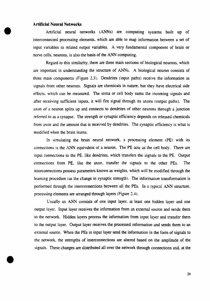
Regard to this similarity.. there are three main sections of biological neurons, which
are important in understanding the structure of ANNs. A biological neuron consists of
three main components (Figure 2.3), Dendrites (input paths) receive the infonnation as
signaIs from other neurons. Signais are chemicais in nature. but they have electricaI side
effects. which can he measured. The soma or cell body SUffiS the incoming signais and
after receiving sufficient inputs. it will fire signal through its a.'(ons (output paths). The
a.'(on of a neuron splits up and connects to dendrites of other neurons through a junction
referred ta as a synapse. The strength or synaptic efficiency depends on released chemicals
From axon and the amount thar is received by dendrites. The synaptic ~fficiency is what is
moditïed when the brain learos.
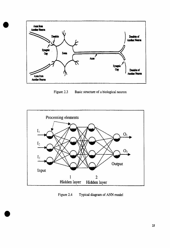
[n simulating the brain neural network. a processing element (PE) with its
connections is the Al'IN equivaIent of a neuron. The PE acts as the cell body. There are
input connections to the PE. like dendrites.. which transfers the signais to the PE. Output
connections from PE.. like the axon. transfer the signais to the other PEso The
interconnections possess pararneters known as weights.. which will be modified through the
leaming procedure (as the change in synaptic strength). The information transformation i5
performed through the interconnections between aIl the PEso In a typicaI ..-u'fN structure.
processing elements are arranged through layers l,Figure 2.4.).
Usually an A1'lN consists of one input layer. at least one hidden layer and one
output layer. Input layer receives the information from an external source and sends them
to the network. Hidden layers process the information from input layer and transfer them
to the output layer. Output layer receives Ûle processed informalion and sends them to an
external source. When the PEs in input layer send the information in the form of signals to
the network.. the strengths of interconnections are altered based on the amplitude of the
signais. These changes are distributed ail over the network through connections and. at the
24
•
s ./);ac DedileofAnadIIrNaD
Figure 2.3 Basic stnlcture of a biological neuron
Processing elements
1-----.Ir • ~A~~'~
Input
lHidden layer
2Hidden layer
Output
0,
•Figure 2.4 Typicai diagram of AJ.\fN model
25
•end. manifest themselves in the forro of outputs. One important characteristic of ANN is
that it processes information numerically rather than symbolically. The network retains irs
information through the magnitude of the signais passing through the network and
interconnections between processing elements.
Figure 2.5 shows the basic structure of a proeessing element and its connections.
The inputs into /h layer are basieally the outputs of the previous layer processing elements
as an input vector. a. with components ai (i=l to n). The output of proeessing element (hj )
is the result of a transfer funetion (j) over a summation of inputs multiplied by weight
parameters and addition of a bias value (1j). Transfer function can be varied depending on
the nature of the data. The most common transfer functions in solving non-lïnear problems
are sigmoid funetion and hyperbolic tangent. A sigmoid (S-shaped) function is depieted
mathemmicully as fol1ows:
1j(:c) =--
1+ e- l(2.13)
This funetion varies between 0 (aLtr=-oc:) and 1 (at x,=+OC). Sigmoid functions. due to their
limiting values. are known as threshold functions. At very low input values. the threshold
function output is zero. At very high input values. the output value is one.
Hyperbolic tangent functions aIso typieally produce well-behaved networks. This
function also has two limiting boundaries of +l and -1 :
t -le -e[(x) =tanh( x) =---
et +e-\(2.14)
•
As the response of this funetion includes bath positive and negative region. their
application are recommended for data set with negative and positive output range
1Swingler. 1996).
Development of an artiticial neural network model
An imponant factor. wrnch distinguishes different neural networks. is the method of
setting the values of the weights or training the network. In training~ AL'1Ns generally cao
26

•
Input variables
Output = f(L"<j.Wi) +8..
•
Figure 2.5 Diagram of a processing element and related calculations
27

•
•
either be supervised or unsupervised. In supervised training~ there i5 an associated output
aIong with any input vector in training data set. Therefore. the weights are adjusted
according to the target output. The most common application of this method is in
classitication.. prediction.. and pattern association problems. On Lqe other hand. in an
unsupervi5ed learning, a sequence of input vector is provided but no target outputs are
specitïed. The network will act in a self-organizing manDer to modify the weights 50 that
mos[ similar input vectors are assigned [0 the same output (or cluster) unit. As the
detinition reveals. unsupervised learning i5 mostly applicable in data clu5tering problems.
Besides the mentioned classification. in each group. there are severa! algorithms of
training. Backpropagation is one of the most applicable algorithm5 in problems involving
mapping of a given set of inputs ta a specified set of turget outputs (Fausett. (994).
Backpropagarion ulgorithm is simply a gradient descent method ta minimize the total
squared error between the output computed by the network and target output. There are
three main stages in backpropagation algorithm: a feedforwurd of the input training pattern.
calculation and backpropagation of associated error and adju5tment of weights with respect
to calculated error. Althou~h the trainine of AL'lN model i5 rime consumin~. a trainedy ~ ~
network will only apply a feedforward phase to compute the associated output and renders
chis phase very rapidly.
The major task in training a network is to bring the network to a balance between
memorization and generaIization. ~lemorization i5 the ability of the network in correctly
responding to input vectors used in training. Generalization is the ability of network ta
respond ta input vectors in the domain of training vectors but not identical to input vectors.
A proposed procedure for achieving this goal applies two disjoint sets of data known as
training and testing data sets. Training data set is used to updating of weights: however~ at
intervals during training. the network is tested with testing data. As long as the network
errer for testing data is decreasing~ the training continues. When this errer begins to
increase the network stans to memorize the features in input pattern too specitïcally and
loses its generalization ability therefore at this point the training is terrninated.
To develop an optirnized networ~ the number of hidden layers and processing
dements in each layer should he selected carefully. In addition to structure of network.
relared pararneters to irnprove the leaming task should he optimized. Two of these
28
•
•
important factors are momentum and learning rate.. wnich control how effectively
backpropagation trains the network (Baughman and Liu.. (995). The learning rate is a
positive constant and controls the rate at which the new weight factors are adjusted based
on the calculated gradient descent correction terro. The momentum coefficient is an extra
weight added onto the weight factors that accelerates the rate at which the weight factors
are adjusted. helping the network to avoid the local minimas. A well-optimized network
has the ability of extracring the relationship between the training data set and adapting its
internaI structure based on related information.
Applications of ANN in Food Science and Agriculture
~[any problems encountered in food.. agricultural and biological industries lend
themselves to a neural network solution. The application of A.NN in different problems is
introduced.
One of the tïrst applications of neuro-eomputing in food technology was introduced
by Thai and Shewfelt (1991). The combination of neuro-computing and statistical
techniques was used to determine the most relevant factors in relating sensory judgment by
human and physical measurements of extemal color of tomato and peach. In this study'.. the
application of neural networks was faster compared to statistical techniques for having
fewer sœps in analysis step: however. statistical techniques were slightly more
advantageous for higher accuracy. Consequently.. neuro-computing technique were applied
to get [he basic features of [he relation: and stutistÏCal techniques were used to improve the
numerical accuracy of resulting mathematical functions. With respect to this study and
above mentioned procedure. the relationship bet\veen sensory evaluations and physical
measurements of tomato and peuch were identified as particu[arly linear.
Bochereau et al. ( (992) applied neural network technique as a parr of procedure for
prediction of apple qualiry using Near Infra-Red (NlR) spectra data. In order to reduce the
nurnber of input parameters and excluding uncorrelated inputs to the neural networlc modeL
principal component analysis (PCA) was appliecl A multiple regression analysis was then
carried out to derive the best linear estîmator and finally the neural network model was
developed to exrract the non-tinear function input and output components. The final result
29

•
•
was a model for predicting the apple quality From NIR spectra. ANN modeling resulted in
5 % increase in accuracy of the linear model with R2 equal ta 0.82
Linko and Zhu (1992) studied the potentiaI of ANN techniques to construct an
appropriate real-rime state estimation and prediction model applicable ta process control in
glucoamylase fermentation. In comparison with conventional modeling, ANN had the
abiliry of handling uncertainties~ complexity. noise and unavailability of data. which are the
common cases in the biochemical reaction analyses. The most related on-Hne data as
oxygen consumption rate (OCR). carbon dioxide evollltion rate (CER) and the nitrogen
utilization rate (Nù"R) along with other inputs were applied to estimate the enzyme activity
and biomass in on-line control. The ANN models had the advantages of ease of use
wirhout a prior knowledge on the complex mechanism of microbial physiology or on the
interrelationships of the variables. Once trained on a typical example data. it .~~~ model
could suppress the noisy dara. The developed A1~~ model performed very satisfactory and
compared weil with real values from off-Hne analyses.
A~'t')i models were applied as a quality prediction model for black teu and resin
samples based on data From chromatography and sensory information (Tomlins and Gay.
1994). Although multiple regression techniques were more aCCllrate compared ta Ai'IN
modeling. the results of A.NN model were improved by reducing the training variables
assigned by srepwise multiple regression. In addition. A4'ms for cases in which the
accuracy is not important (for example in quality control) provides more advantageous
application in predicting severa! parameters simultaneously. The combination of statisticaI
procedures and A1'IN were suggested as useful tools in pattern recognition and regression
of chromatographie (GC and HPLO and sensory data.
Park et al. (1994) applied an Al'fN model for predicting and classifying beef
characteristics using ultrasonic spectral feautures as the input data for training the models.
A.'N models provided becter results compared to statistical regression models for
predicting the sensory attributes of beef as juiciness. muscle fiber tenderness. connective
tissue. overall tenderness and tlavor intensity. The relationships between physical
attributes and sensory properties were mostly linear as an Ai'fN model developed without
hidden layers performed best. The accuracy of ANN mode1 for classification were a
function of learning schedules. number of processing elements in hidden layer and number
30
•
•
of input variables. Increasing the ultrasonic spectral fearnres as input variables increased
the accuracy of classification.
Sayeed et al. (1995') investigated the possibility of an ANN model development for
sank quality evaluation. For this purpose a machine vision technique was applied to
quantify the quality features of typical snack products in the forro of texture (reflecting the
internai structure) aIong with size and shaPe fearnres. The relationship between the
mentioned variables and sensory attributes were not adequarely linear as examined by
linear regression. merefore the input variables were applied to train a backpropagation
Al'IN model to leuro the non-linearity between input and output variables. The developed
ANi\' model was validated with a set of untrained data and the prediction results were
compared to those from a taste paneL The developed methodology had a potential
application in snack production industry as a non-destructive method of quality evaluation.
The potential A1~N models for milk shelf-life prediction was evaIuated by Vallejo
Cordoba et al. (1995). Dynamic headspace gas chromatographie data collected during the
storage of pasteurized milk were applied as input to he reluted to tlavor-based shdf-life of
milk in days as dependent variable. A~'fN and Principle Component Regression (PCR)
techniques were used and compared for their predietability. A.l\fN. with 2-day standard
error in shelf-life prediction. performed better that the 4-day error PCR technique. and
indicated a higher predictability for chis concept.
Sablani et al. (1995) investigated the potential of .'-\l'IN models for prediction of
optimal sterilization temperarures. A finite difference model generated the data for a set of
assigned conditions (can size. thermal diffusivity and kinetic parameters of quality factor)
ta obtain the associated sterilization temperarures. Afterwards the optimum conditions and
relared quality factors were applied as inputs to train the AJ."~ mode!. The trained madel
was able ta predict the optimal sterilization temperarnres with less chan 5% error. In
artempt to predict the overaIl heut transfer coefficient and fluid ta particle hear trafisfer
coefficient using Al'lN modeling technique. Sablani et al. (1997) obtained significantly
superior results compared to dimensionless correlation techniques. Beside the higher
aecuracy of prediction. ~'iN models were more versatile man dimensionless number
models.
31

•
•
Rauan et al. (1997) compared the predietability of ANN models for rheoligical
properties of a coolde dough. The raw input data were obtained from mixing power
consumption curves. The investigated rheologieal properties were farinograph peak.
extensibility and ma'<imum resistance. Two speetrum analysis techniques. Fast Fourier
Tr~nsform (FIT) and power spectral densiry (PSD) were used for data preproeessing as a
part of .-\l~ model development. Using these techniques the raw data (time domain data)
were converted into frequency domain data. The above-mentioned techniques improved
the training abilitv of Al.'IN models for reducing the noise and size of the initial raw data... - ...and \Vere recognized as successful techniques of data preprocessing in this study.
Ghazanfari et al. (1996) studied the suitability of multi-structure neural networks
(~ISl\rN) over a single multi-Iayer neural network (NrL~) for classification of pistachio
nuts. The yIS~~ classitier was constructed from four single Ai'IN models. which were
[rain~d separately with one output variable from each network representing one variety
(class) of pistachio nuts. The input data for these madels were physicaI attributes of nuts
derived from their images. The c1assitication accuracy of developed NIS!'4N was compared
with y[L~N modeI. The MSNN technique significantly increased the classitïcation
performance. In addition. ~ISNN had the advantage of smaller network architecture.
which is more preferable for hardware and software implemenration.
.-\ngerosa el al. (1996) developed an Al'1i madel as alternative ta sensory
evaluation performed by a taste panel for virgin olive oil by panel test. A wide range of
samples tcovering different variery. quality. ripeness. sanitary and geographicaJ ongin) was
subjected to a sensory evaluation by a taste panel. The results of quantification of volatile
fractions using headspace gas chromatographie technique were used as input data to predict
the panel test scores (output variables). The ANN mode1 was able to generalize the
relationship between these two sets of data successfully with a high degree of aceuracy.
5uggesting the substitution of developed A.L\lN model with panel test.
Briandet et al. (1996) applied ANN technique as one of alternative statistical
approaches for correlating data from Fourier transform infrared (FrIR) for detection of
adulterated freeze dried instant caffee. This FI1R technique was applied as a rapid
alternative to wet chemistry methods~ however~ data analysis of this technique were more
complicated. AL"'N models were compared to principle component regression and partial
.....,-'-

•
•
least square regression.. and the superior perfonnance and generalization potential of Ai'JN
model was demonstrated with an independent set of data with 100% correct classifications
ability.
Pamer ec aL. (l997) developed an AJ.'IN mode1 [0 evaluate the factors involved in
the contamination process and aIse the significant factors in the magnitude of aflatoxin
contamination of in preharvest peanuts. Alternative to ANN model. a stepwise traditional
regression model was developed for this purpose. The input variables (soil temperature..
drought duration. crop age and accumulated heat units) were related to at1atoxin levels.
This study showed the ability of A1'lN models for this purpose in addition ta better
performance than Hnear regression technique.
Kim and Cho (1997) applied three developed Al'lN models as a part of a fuzzy
controller in bread baking process. For this purpose three main parameter in bread baking
process namely volume. browning and temperature were measured in 3 seconds and :!
minutes intervals. resulting in training data for 3 AJ.\fN model development. The neural
networks showed a good performance for predicting temperature. volume and browning.
The knowledge from developed models and an experienced operator \vere used ta detïne
[1 mies for fuzzy controller. Using a fuzzy contro[[er instead of a human operator can
reduce the cast of heating of the oven.. withont the loss of bread quality.
•o.\1\j~ models as an alternative in data-processing technique to partial least squares
(PLS) and principle component analysis (peA) showed better prediction ability (Horimoto
el al.. 199ït In order to classify the tlavor quality of milk as a part of qualîty control.
dynamic hcadspace gas chromatographie was used to quantify the off-flavor components.
UHT milk \Vas inoculated with various bacteria! species and storage rimes. The content of
training and testing data as weil as optimized parameters.. which were related to Al'lN
model development (learning rate. momenturn factor and hidden PEs). intluenced the
predictive ability model.
During ~sobaric-isothermal inactivation of ex-amylase enzyme. pressure and
temperature had a complex effect (Geeraerd et al.. 1998). A model based on Arrhenius Iaw
presented a non-lïnear description of the system. Due to lack of data. an A1~ model was
applied with respect to its ability in prediction of complex systems. The ANN model was
able to predict the complex effect of pressure and temperature on the inactivation rate
33

•
•
constant using a limited set of experimental data. The effect of transfer funerion of eaeh
neuron was believed to be imponant in a low complex Al'IN model development.
Gebri et al. (1998) applied Ai'lN modeling in predieting the origin of white vinegar.
Among different chemico-physieal and sensory analysis. seleeted parameters such as
polyalcohols. pH. tartane acid and proline had the Most reliable rule in discrimination of
the product. A broad data set covering products from a variety of raw materials and from
various countries subjected ta multivariate statistical analysis were used ta develop the
.~'N model. The Ai~~ model was able to predict the botanical origin of the product and
also was able to re-elassify products with unknown origin.
The above review indicates the status of available methods of process calculations
1with sufficient scope for developing new method. which can reduce process calculation
errors 1. as \vell as the poœntial of Al'lN models for use in process calculations. The present
thesis aims at developing an ANN based process calculation model. which would be more
versatile and accurate chan the existing methods.

•
•
CHAPTER3
Al'N S~IlJLAnON OF BALL Al~DSTmmo FORMULA ~IETHODSOF THEIUtIAL
PROCESS CALCULATIONS
ABSTRACT
Application of Al'lN models to simulate BalI and Stumbo methods of thennal process
caIculaùons i5 presented in this srudy..ANN models were developed based on relating Bali and
Srumbo table parameters to facilirate process calculations. The A~\lN models related g value (as
a measure of process [Îmel [0 fiIU (as a measure of process lethality). Tables developed by
Stumbo accommodate the jd: (cooling lag factor) while relating g and JilU. therefore. for
devdoping :\~N models of Srumbo metbod, jn: was also considered as an additionai input
variable. The developed fu~'N models for BalI and Srumbo methods were validated using a new
set of processing conditions. involving a range of retort temperatures. initial temperarures.
heating roltes and heating lag factors [and additionaIly. for Stumbo method. cooling lag factors
lj,,)}. The prediction eftïciency of .~'lN models were a function of the size of training data set.
number of hidden Iayers and PEs in each hidden layer as weIl as other leaming pararneters.
.--\."~ based Bali models had an average error of 1% for the validation data set while the AJ.~~
based Stumbo models had a slightly higher 3% average error for process time and process
lethaIity calculations. The smaller size of data set and a wider range of parameters associated
with Stumbo tables were considered to be the reason for the associated higher errors with the
.-\1'"N based Stumbo models. In generaI. the Al\lN models were considered ta simulate BalI and
Stumbo methods of process calculations weil providing a basis for further exploration of the
concept.
35
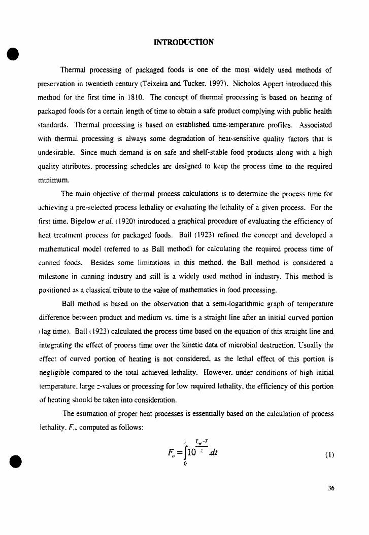
•INTRODUCTION
Thennal processing of packaged foocis is one of the most widely used methods of
preservation in twentieth century (TeL'<eira and Tucker. (997). Nicholas Appert introduced this
method for the first time in 1810. The concept of thermal processing is based on heating of
packaged foods for a certain length of rime to obtain a safe product complying with public health
standards. Thermal processing is based on established time-temperature protïles. Associated
with thermal processing is aIways sorne degradation of heat-sensitive quality factors that is
undesirable. Since much demand is on safe and shelf-stable food products aIong with a high
quality attributes. processing schedules are designed to keep the process rime to the required
mInImum.
The main objective of thermal process calculations is to detennine the process rime for
Jchieving a pre-selected process lethaIity or evaluating the lethality of a given process. For the
tïrsr üme. Bigelow et al. t 1920) introduced a graphicai procedure of evaluating the eftîciency of
heat treatment process for packaged foods. Bail (1923) retined the concept and develaped a
mathematical model (referred ta as BalI method) for calculating the required process rime of
canned food~. Besides sorne limitations in this method. the BalI methad is considered a
milestone in canning industry and still is a widely used method in industry. This method is
positioned a.'i a classical tribute ta the value of mathematics in food processing.
BalI method is based on the observation that a semi-logarithmic graph of temperature
difference between product and medium vs. rime is a straight line after an initial curved portion
(lag rime). Bali t 1923) caIculated the process time based on the equation of this straight line and
integrating the effect of process time over the kinetic data of microbial destruction. LTsuaIly the
effect of curved portion of heating is not considered. as the lethal effect of this panion is
negligible compared ta the total achieved lethality. However.. under conditions of high initial
remperature. large :-values or processing for low required Iethality. the efficiency of this portion
of heating should be taken into consideration.
The estimation of proper heat processes is essentially based on the calculation of process
lethality. F. .. camputed as fallows:
•c Trpf-T
F =JI0--;- .dttJ
o(l)
36
where:
• T~t: reference temperarure
T: ~enter point temperarure
z: temperature sensitivity indicator of F value.
For law acid food products. 250~ (l21.1')C) is widely used as a reference temperature. BalI
deveIoped tables and graphs (0 relate process rime and process lethaIity. These tables and graphs
\Vere based on relating two parameters: g (temperature difference between product and heating
medium at the end of heating) as a measure of process rime (0 Jill} (ratio of heating rate to
srerilization value) as the measure of process lethaIity. Sorne restrictive assumptions were made
Juring the development of these tables and graphs. One of the most important parameters. which
~~m somerimes cause crrors in calculations.. was a constant cooting lag factor. jn value.. equal to
1A1. Therefore. BaIl method overestimates process lethality when ix< lAI and underestimates
when jll> 1Al (Bail and Oison.. 1957: Hayakawa. (978). Also.. BalI (1923) assumed an equal
heating and cooling rate tJir=ll. In practice.. the values of these two parameters differ from each
tlther. It has becn found that for steam heating and water cooling j;.-1.3Jir (Pham.. 1990) and
L)bviously disregarding this inequity interferes with the accuî~cy of process calculations. BalI
method has been wide[y reviewed and evaluated by several researchers (~[erson et al.. 1978:
Rambert et d/. .. 1977: Steele and Board.. 19;9: Spinak and WiIey. 1982: Stoforos. 1991).
Stumbo and Langley <.1966) reviewed and revised tables developed by Bali 11923). The
variability of il- value was considered in these tables for more reliable and accurate thermal
processes calculations (Stumbo. (973). These tables are obtained from hand drawn heat
penetration curves and relate JiIU and g values with respect to variability of i:c- Also the
variability of 1;, and l· was considered in developing these tables. but it applies only to cases
where the difference ofth and f~ is not more than 20% of respective.th value 1Hayakawa. 1978..
Stoforos el al.. (997).
ArtificiaI Seural ~etwork~Iodels
Artitïciai Neural Setwork (Ai'lN) rnodels are computationai models made up of several
processing dements l PEs).. which are connected through weighted links.. Development of model
•37
is basically based on adjusting the weights through presenting adequate number of examples
• consisting of input and output variable pairs.
GenerJ1ly Ai\iN models are constructed from an input layer. an output layer and one or
more hidden layerts). Input layer tr'ansfers the information ta the network for proeessing.
Output layer receives the processed information and sends it to extemal receptor. Hidden layers
process the received information from input layer. extraets the existing features in input variables
and predict an output. Among different networks. back-propagation network has the mose
applicability in prediction and classification problems. Baekpropagation network is a feed
forward network. which propagales back a portion of error between desired and ANN predieted
output ta correct the weight pararneters.
Recently. ANNs have shown a potential for applications in food science and technology
areas. Eerikainen el al. (1993) presented a series of examples of potential application of AJ.'lN
modds in food-related applications. Parmer er al. (1997) applied neural network modeling for
~stimation of atlatoxin contamination in peanuts which performed better than trnditional linear
regression techniques. ~i and Gunasekaran ( 1998) simulated the complex task of food quality
prediction using .·\NN models. Boucherau el al. (1992) developed a neural-network-based
method for prediction of apple juice quality using near infrared spectra. Neural networks were
used to detennine the significant variables in harvesting and processing effects on Surimi quality
by Peters t!C ul. ( (996). Kim and Cho (1997) developed an .o-\i~~ model for the bread baking
process. using three quality factors of volume. browning and temperature. In thermal processing.
Sablani et al. t (995) applied neural network models to predict optimum thennal processing
~onditions. As an application in drying. Sreekanth el al. (1998) developed an A..'iN mode1 for
prediction of psychometrie parameters.
The global objective of this study was ta evaluate the potential of A.L'IN models as an
alternative [0 conventional process ealeulation methods. As a first step in this direction. data
from two dassical methods: BalI and Stumbo methods. were used to develop the .o.\i~ models
and assess rheir perfonnanee. Renee. the specific objective of this paper is fu\fN simulation of
Bail and Stumbo formula methods of process calculations.
•38

•
•
~IATERIAL AND ~IETHODS
ANN modeling of Bali and Stumbo methods
Bail and Stumbo methods relate process time and pracess lethality by employing t\va
parameters. g andfJlU. in the form of tables or graphs. In tables developed by Stumbo. the effect
of jn on this relation is aise considered. For a known process time aIong with the other
processing conditions. g-value will he known; altematively for a given process lethality.f,/U will
be known. For developing A1~~ based process calculation models. Bail and Srumbo methods
were simulated based on relating the parameters of these tables. Data (jilU vs. g or g vs. f,;u) for
both training and verification were obtained from tables published in Lapez (1987) for BaIl
method and Stumbo ([973) for Stumbo method. Detailed tables were available in Lapez (1987)
and hence 1050 data pairs were used in Bali model for training. For Stumbo method. only 44
data sets relatingjilU vs. g (and vice versa). were available al 9 different values of jl..l. A :-value
ùf IOC was used for both models. For each method. two modeis were developed one for
predicting.tilU ba."ied on g. and vice versa.
Development of .-\~N models
Bail model
~eural\Vorks Professionai WPlus.. version 5.23 (~euraIWare me.. Pittsburgh. PA) was
~mployed for :\J.~~ modeling. .~ standard back-propagatian algarithm with tangent hyperbolic
transfer functian and narmalized cumulative delta learning rule was applied as the basic
architecture of nt=twork. As the input and output variables had a broad range. for a better
presentation of input and outputs ta the network and a more uniform data set. a mathematical
transfonn function \Vas applied. Therefore. log g was predicted From [og(j'/u). and liIU in the
fonn of arctangent([og /,./U) \Vas predicted From log g. For a more convenient recalling of
models. from now prediction of log g will he denoted. as Madel A and prediction of f,;rJ will he
denoted as ~[odel B.
It has been recognized that the network predictability and performance should be
optimized wîth respect to the size of the training data set. structure of the network. number of
hidden Iayers. number of processing elements in the hidden layer. type of learning rule and
trmsfer function. Severa! other variables aIso affect the ANN model development and
39

perfOl1nance. Among them momentum and epoch size have the most significant effect on the
• network performance. The momentum represents a fractional value from the previous weight
change added to the present weight correction. Its value can change between 0 and 1. however.
higher momentum values speed up the leaming process and prevent the model from being
trapped in a local minimum. At the same rime. large values of momentum will cause large error
oscillations 1NerualWare. 1996: Baughman and Liu. 1995). Epoch is the number of training
presentations between weight updates. This method of updating weights which increases the
convergence speed is known as cumulative delta mie leaming. However. using cumulative
deita-rule learning for updating weights will require more calculation and. if the epoch is too
large. the advanrage of using overall error function can be lost Therefore. depending on the
problem. the epoch size should be optimized.
The perfonnance of an ANN model is intluenced greatly by the quantity and quality of
dam llsed as the training set (Linko and Zhu. 1992). The training data should have suftïcient
information to describe relation between input and output variables. A correct format of input
~nd output variables could increase the leaming ability of AJ.'INs by detecting and extracting the
relation between input and output variables (NeuralWare. (996). This stage of Al'IN models
deve(opment is thus regarded as data preprocessing~which could be petformed in different ways
to improve the model efficiency llaeroix er al.. 1997).
Keeping the above constraints in mind. to select the required number of examples in
tr~ining set. a leaming curve was developed. The original data l 1050 dataI were sorted from the
lowest [0 highest value. To have six equal groups of data. every seventh data row was selected
and removed from the original set. These fonned the tïrst <Group Al data set of 175 data points.
The same procedure was repeated with the remaining data until six homogenous groups (A ta F)
of data each with [75 data points were obtained from the original data. Each of the group thus
covered the entire range of data in original set. Different combinations of these groups were
used ta achieve different sizes of training and testing data sets. These arrangements are shown
in Table 3.1. The data sets that were not used for trainini! were used for testing durin~... --development of model. The developed models were tested also with ail the available data from
the original data set ta evaluate the consistency of performance. This procedure was followed
for both models lA and B).
•40
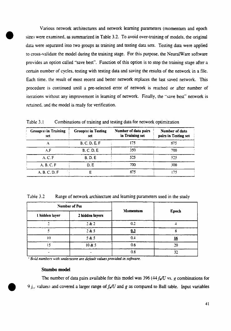
Various network architectures and network learning parameters (momentum and epoch
• size) were examined. as summarized in Table 3.2. To avoid over-training of models. the original
data were separated into two groups as training and testing data sets. Testing data were applied
to cross-val idate the model during the training stage. For this purpose. the NeuralWare software
provides an option called ··save besf·. Function of this option is to stop the training stage mer a
certain number of cycles. testing with testing data and saving the results of the network in a file.
Each rime. the result of most recent and better network replaces the last saved network. This
procedure is continued until a pre-selected error of network is reached or after number of
Iterations without any improvement in leaming of network. Finally. the "save besc" network is
retained. and the model is ready for veritïcation.
Table 3.1 Combinations of training and testing data for network optimization
Grouplsl in TfOlining GroupfsJ in Testing Sumber or data pairs Number or dataset set in Training set pairs in Testing set
.-\ B.C.O.E.F liS 875
A.F B. C. D. E 350 700
A.C.F B.D. E 5~ 5~
A. B. C. F D.E 700 300
A.B.C.D.F E 875 175
Table 3.2 Range of network architecture and learning parameters used in the study
Sumber or Pes~(omentum Epoch
1 hidden layer 2 bidden layers
2 2&1 0.2 ~
5 2&5 0.3 8
10 5&5 0..1 16
15 10&5 0.6 10
- - 0.8 32
" Bold numbers .,,-[(Ir rmderscore are default values provided in software.
Stumbo model
The number of data pairs avaiIable for chis modeI was 396 (44t,.;rJ vs. g combinations for
• 9 j( f' values) and covered a Iarger range of[JIU and g as compared to BalI table. Input variables
41
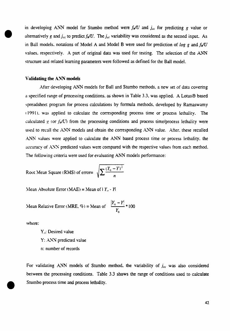
• in developing A~~ model for Stumbo method were fiIU and jc.'C: for predicting g value or
altematively g andjcc to predictf,;lJ. Thejc:c variability was considered as the second input. As
in Bali modeIs. notations of ~Iodel A and Madel B were used for prediction of log g and f,/U
values, respectively. A part of original data was used for testing. The selection of the Al'lN
structure and related learning parameters \Vere followed as defined for the BaIl mode!.
Validating the ANN models
After developing A1~~ models for BalI and Stumbo methods. a new set of data covering
a specitïed range of processing conditions. as shown in Table 3.3. was applied. A Lotus® based
spreadsheet program for process calculations by fonnula methods, developed by Ramaswamy
1 1991). was applied to caIculate the corresponding process time or process lethaIity. The
~alculared g (or ji/V) from the processing conditions and process time/process lethality were
used ta recall the ..\J.\IN models and obtain the corresponding A.l.~~ value. After. these recalled
.-\1\fN values were applied ta calculate the .-\l'IN based process time or process lethality. the
accuracy of .-\..'i~ predicted values were compared with the respective values from each method.
The following criteria were used for evaluating Al'fN models performance:
I~(r:)-y):'Root y[ean Square (RJ.v[S) of error= V~ n'
~[ean Absolule Error (NIAE) =Mean of 1Yt , - YI
y[ean Relative Error ~~'1RE. %) = ~Iean of
where:
y,): Desired value
Y: .~'i~ predicted value
n: number of records
Ir _yi
l} 1 *100Yo
•For vaIidating ..~'IN models of Stumbo method. the variability of j,x was aIso considered
between the processing conditions. Table 3.3 shows the range of conditions used to caIculate
Stumbo process rime and process lethality.
42

Table 3.3 Range of parameters for validaring A1'lN based BalI and Stumbo models
• Parameters BaU Stumbo
RT (oC) 115-125 110-130rr (oC) 65 70-90
fh (minI 10-20 23-[85
Jch 1.2-2.0 1.80-2.04
Jec lAI 1.70-2.00
Process letha1ity (min) 5-64 5-15
Process rime (min) 13.7-147 25-400
RESULTS AND DISCUSSION
A~N based Bail ~[odel
•
:\Iodel development and optimization
Ir has been recognized that the network predictability and performance is dependent on
the nature and size of training data set. strucmre of the network and sorne relevant pararneters
during training. Training data set should ideally cover the desired range of problem and consist
of ~nough records to let the network leam the features. Al'1N models learo trend From the data in
training data set. This capacity is based on the number of processing elements (PE) or more
specifically number of connections. [f the number of PEs are more than what is needed with
respect to training of the model. the network may lose the generaIization ability and begin to
memorize the data which is mostly undesirable (NeruaIWare. 1996).
A well-trained network is optimized between generalization ability and Iearning the
trends in training data set. To prevent the memorizing problem~ a separate data set from training
data should normally be selected randomly and this data set will be applied during training stage.
After certain number of cycles. the training is stopped and the testing data set is used to calculate
the error. After the network has converged to or reached a minimum global error. the training
can be stopped.
For developing the Ai'1N-based Bail mode!. the first objective was to choose the correct
size of the training set. which ensured the Iearning and generalization ability of network
43

simultaneously. Figures 3.1 and 3.2 illustrate the effect of number of examples in training data
• set based on recalling training data set (as a measure of network ability to learn the data). as weil
as testing the network with testing data which were not used in training data set (as a measure of
generalization ability of network). Also. each network model was tested with the entire original
data set and the combined results are shown in these graphs. For both models. the errors
associated with training and testing data sets were very close for each training set size.
demonstrating the potentiaJ ability the of network for generalization. The results also confirm
that the !!eneralization abilitv of network was not affected bv trainin~ data set. However. the size......, . .....
of the training set had a signitïcant impact on the prediction ability of network. At the lowest
level tried. the CITors were quite high. For the Ai'IN based Ball-method. a training data set of size
containing as many as 175 data points could be accommodated because of the availabiIity over
1000 data points in the original set. And even at this size. the associated errors were high and
converged to lower values only after the size was increased. The network had minimum errors
with a size of 525 data points which was se[ected for both models (A and B). the remaining
being used exclusively for testing.
Th~ error parameters for selecting the required number of hidden layers and PEs in each
hidden layer are shown in Table 3.4. Changing the number of PEs in networks. with one hidden
layer. generally resulted only in a smaii improvement in performance. However. the addition of
a second layer. markedly improved the prediction ability. which was more significant for ~lodel
B than for NIodel A. Increasing the number of hidden layers ta 3 did not result in uny advantage
l)Ver the model with 2 hidden layers. but increased the computation rime. H~nce. ~lodel A was
selected with 1 hidden layers and 2 PEs in each layer. and a 2-hidden layer network with 5
processing elements in each layer was assigned for Madel B. It has been generally recognized
that assigning the appropriate number of PEs and hidden layer(s) is mostly a trial and error
m~thod. however. two hidden layers for most of problems is sufficient (NeuraIware. 1996).
•

•0.012
0.01
0.008
~
-< 0.006~
0.004
0.002
0175 350 525 700 875
Number of examples in training set
.Training OTesting .Testing W/I050
Figure 3.1 Learning curve for ANN model A (prediction log g)
0.006
0.005
0.004
;:;< 0.003~
0.002
0.001
0175 350 525 700 875
• Figure 3.2
Number of ~xamples in training set
.Training DTesting • Testing W/I050
Learning curve for Ai'lN model B (prediction/JIU)
45
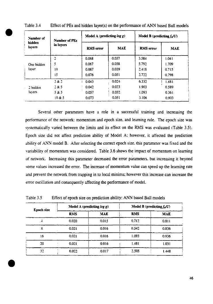
0.361
0.903
1.09J
3.106
0.032
0.051
0.057
0.073
Effect of PEs and hidden layer(s) on the performance of ANN based BalI models
la~ers
Table 3.4
1 Model A (predicting log g) ~[odd B (predictingf,.lu)~umberor
Number of PEs!
hiddenin layers
i layers Rl.\lS error ~[AE ~[S error MAE
2 0.068 0.037 3.584 1.041 1
On~ hidd~n 5 0.067 0.038 5.792 1.709
1
layer 10 0.067 0.039 2.418 0.715
15 0.076 0.051 2.722 0.7981
2&2 0.043 0.024 6.332 ! 1.~81!i 1
1 hiddcn 2&5 0.0421
0.023 1.903 0.589. , - - 1 ....
•
S~veral other parameters have a role in a successful training and increasing the
performance of the network: momentum and epoch size. and leaming role. The epoch size was
systemarically varied between the limits and its effect on the R.MS was evaluated (Table 3.5).
Epoch size did not affect prediction ability of Madel A: however. it affecled the prediction
abililY of ANN model B. After selecting the correct epoch size. this parameter was tïxed and the
variability of momentum was considered. Table 3.6 shows the impact of momentum on learning
of network. Increasing this parameter decreased the error paramelers. but increasing il beyond
sorne values increased the error. The increase of momentum value can speed up the leaming rate
and prevent the network from trapping in ta local minima: however this increase C3.1l increase the
error oscillation and consequently affecting the performance of model.
Table 3.5 Effect of epoch size on prediction ability: ANN based Bali models
Epochsize~[odel A lpredicting log g) t ~Iodel B (predictingf,.ll;1
R.\[S ~(AE 1 R1\IS ~[AE
0.020 0.015 1 0.712 0.811
8 0.021 0.016 1 0.542 0.836
16 0.021 0.016 1.093 0.936
•20
32
0.021
0.022
0.016
0.011
1.481
2505
1.031
1.448
46
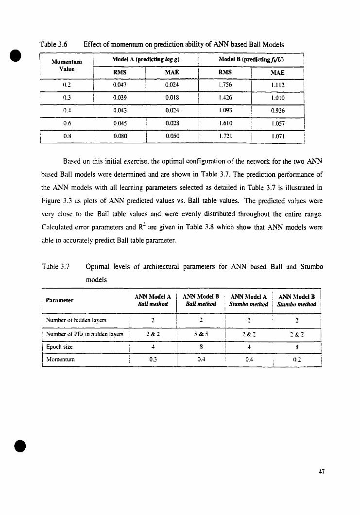
Table 3.6 Effect of momentum on prediction ability of Ai'lN based BalI rvlodels
• ~lomeDtum~Iodel A (predicting log g) ~Iodel B (predicting/tlll)
ValueRMS MAE R.'\1S ~LU:
0.2 0.047 0.024- 1.756 1.112
0.3 0.039 0.018 1.426 1.0lO
OA 0.043 0.024 1.093 0.936
0.6 0.045 0.028 1.610 1.057
0.8 0.080 0.050 1.7:!1 1.071
Based on [his initial e:<ercise. the optimal configuration of the network for [he two ANN
b~lSed BalI models were determined and are shown in Table 3.7. The prediction performance of
the AJ.\fN models with ail learning parameters selected as detailed in Table 3.7 is illustrated in
Figure 3.3 as plots of AJ.\IN predicted vaIues vs. BalI table values. The predicted values were
very close [0 the BalI table values and were evenly distributed throughout the entire range.
CaIculated error parameters and R~ are given in Table 3.8 which show thar .o\1'fN models were
able to accurately predict Bail table parameter.
Table 3.1 Optimal levels of architecrural parameters for ANN based Ball and Stumbo
models
•
ParameterANN ~Iodel A ANN ~lodel8 ANN ~(odeIA &~ ~Iodel B
Ballmethod BaUmethod Stumbo met/rad Stumb(J melhod
~umber of hldden laycrs 2 2 2 2
~umber llf PEs in hidden layers 2&2 5&5 2&2 1&2
Epoch size ..f. g 4- g
~[omentum 0.3 OA OA 0.2
47

2
• ~ .. .. , ..
1
~0
Q
1-1
~2o Table data
+A~ prIIIctedGraphA
-3 1
0 50 100 150 200 250
thIU
2CO ,..----------....,..----_..--.,
150 ~
i 100 ~-
o Table data
+ ANN predicted
•
Figure 3.3
50-
Grpeh B ~0 ".
-3 -2 -1 a 1 2Dg;
Comparison of fu~~ predicted values and BalI table parameters respect to inputvariable
48

ANN BaU ~Iodel A ANN Bail Model BError parameters
Logg Process time /IIU Process lethality
lU.tlS 0.04 0.607 2.48 0.165
~IAE 0.02 0.458 0.66 0.084
~IRE 4.98 1.025 1.14 1.321R- 0.99 0.99 0.99 0.99
ANN Stumbo ~[odel A ANN Stumbo ~[odel BError parameters
Logg Process lime /,.IU Process lethality
R..',.IS 0.08 6.43 3.15 0.33
y[AE 0.06 5.06 1.35 0.241
~[RE 6.13 3.04 2.78 3.03 :
R- 0.99 0.99 0.99 0.99 i
•Table 3.8 Error parameters for ANN based Bail and Stumbo models
•
~Iodel verification
Figure 3A illustrates the results of validation of the developed models with a new set of
data which involved a wide range of operating parameters normally encountered in commercial
thennal processing operations (Table 3.3). The predict.ion error parameters are aiso summarized
in Table 3.8. For bath models (process time prediction. Madel A and process lethaIity
prediction. ~Iodel 8) the R: was close to unity. which showed excellent correlation between the
ANN model and Bali method. The associated mean relative errors for both process rime and
process lethality predictions were 1.0 and 1.3%. respectively. The mean relative error is more
meaningfui with respect to process lethality. while for process time. the mean absolute error (0.5
min) which indicates the error in user units (min) is more easily reconcilable. Over the range of
process time encountered (Up to 150 min). this represents a mean range ~rror of about 0.3%
which was considered smalI.
A~N based Stumbo ~Iodel
The various pre-processing constraints were aIso evaluated with respect to the Stumbo
model aIthough sorne could not he accommodated because of the smaIler size of the available
data. For example. since ooly 44 data pairs were avaiIable at eachj(:c value. the size optimization
49

• 200 r------------------.,
•1 100
lliCD 50ZZ< oANN.lue
20050 100 150
Bail pme•• Ume (min)
OL.----........-----""-----------o
o ANN \fÛue
~ 40 8C ~
Bali pme•• letharlty (min)
'ê"80...------------------...,l~!m1•18 40a-i3!2Q1i<O...~----L-----'-----"--------o
Figure 3.4 Validation of Ai'ffl models of BalI method
• 50

•
•
couId not be done. The required number of processing elements and the number hidden
layerswere optimized based on the RMS of eITors and MAE. Since the quality of data between
these [WO tables (BalI and Stumbo) were similar, optimal conditions with respect ta momentum,
transfer function. and learning mIe were expected ta he somewhat similar ta those achieved in
the .~'lN based BalI model. Aguin. 2-hidden-layer network performed considerably better than
I-hidden-Iayer networks. The optimal conditions for number of PEs were 2 PEs in each layer.
white for one of the Bali models. the best model had 5 PEs in each hidden layer. The appropriate
architecture of networks was also used to select the proper values for epoch and momenrurn. and
these were also slightly different. The differences in the architectural configurations were
considered [0 be the result of smaller size of data set available for Stumbo model. The optimal
conditions are summarized in Table 3.7.
The performance of the A~ based Stumbo models as a plot of ANN predicted value vs.
desired output vaiue is shown in Figure 3.5. The computed errors and the associated R~ values
are included in Table 3.8. The tïgure demonstrates an excellent agreement between predicted
and expected values with a high R1 value. The mean errors \Vere.. however. somewhat higher
than those observed with A1\4~ based Bail models. For Nlodel A. for example. the ~[RE was
6. 1~ for the Stumbo model as compared ta 5% for Bali model for log g prediction and 2.8% and
LI ct. respective[y for ft/U predictions. The differences were considered to be primarily the
resuIt of differences in the size of available data over a wider range of/ilU and the addition of jn:
as a second input. Accommodating these changes probably requires a larger training set. but the
number of data in Stumbo tables were far less chan that in Ball table. It was shawn earlier with
:\.'IX based Bali model that the perfonnance errors were quite high even with the availabiliry of
175 data points. It may thus be logicai ta assume a higher performance error with Stumbo
models.
The results for validating ..:\.L'lN models in the fonn of predicted vs. expected process time
and process lethality is shawn in Figure 3.6. With respect ta process lethality and pracess
lethality predictions. the associated errors (MRE) for Al'IN based Stumbo models. were again
3% while they were about 1% with Al'lN based BalI models. The associated R! were aguin very
high and the quaiity of predictions was excellent. The slightly higher errors with predictions by
the .-\i~ based Srumbo madels were again ascribed ta non-availability of adequate number of
data sets ta properly train and develap the Al'1N models. The associated errors were. however.
51
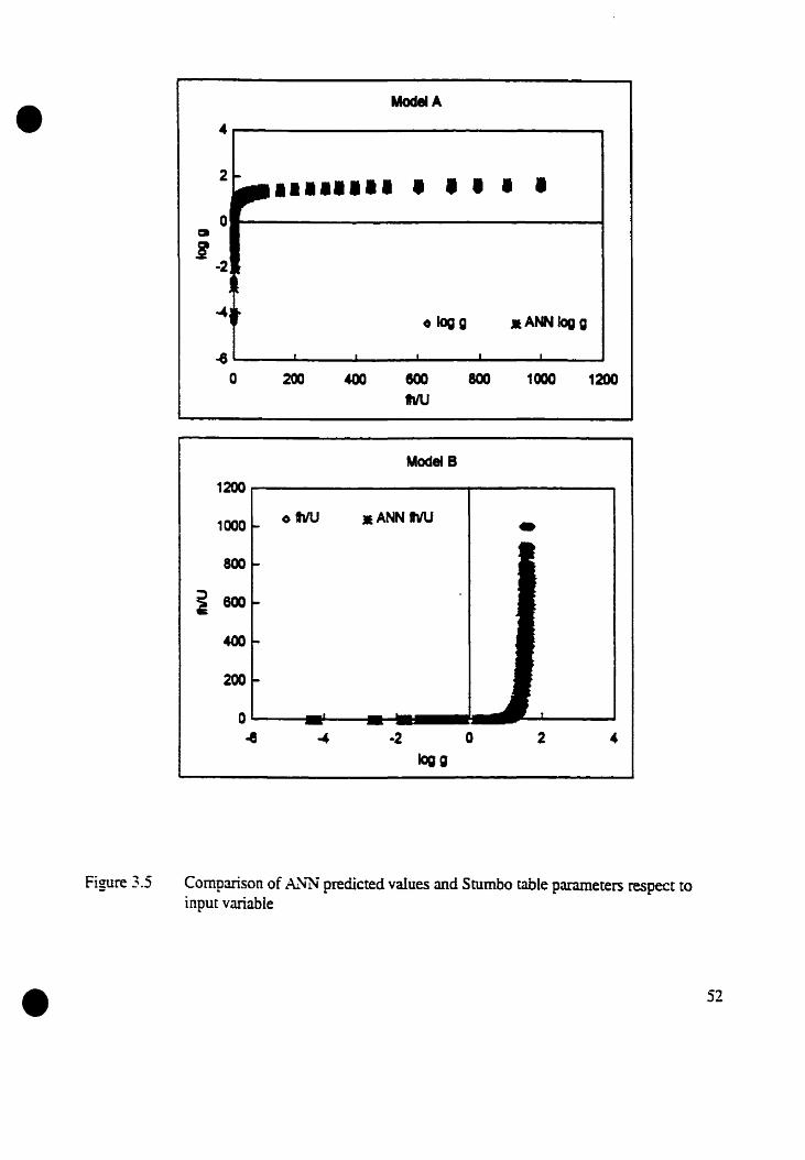
ModelA• 4
2 •••••••• • ,.• •0
ca
1-2
olegg .ANNlogg
~
0 200 600 800 1000 1200l1IU
Model B
1200
1000 o1hlU .ANN thlU -8QO
::)600~
400
200
0..e ·2 0 2 4
Iogg
•
Figure 3.5 Comparison of A..'fN predicted values and Stumbo table parameters respect toinput variable
52
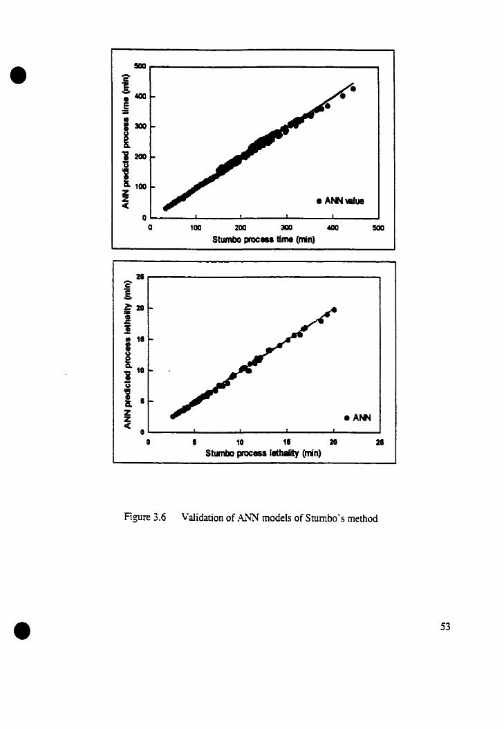
500 ......------------------.••1300l1200Ü=;l5. 100ZZC e ANNWllue
100 200 300 400
Stumbo proc_ lime (nin)
O~----L..---...I..---......I.---""""'--_--'
a
21
eANN
1 10 11 20Stumbo process JethaIity (nin)
o L.....__--L ..L- .......__........ ""'"
a
21-------------------,
Figure 3.6 Validation of .Au'fN models of Stumbo·s method
• 53

considered low enough and demonstrate the utility of the Al~~ concept for simulating BalI and
• Stumbo process calculation techniques.
CONCLUSIONS
The feasibility of A.i~~ modelling for process calculations was evaluated in this srudy
based on their ability to simulate BalI and Stumbo methods. The Ai'lN roodels were able to
correlare the parameters of Ball and Stumbo tables with good accuracy (mean relative errors of
1-3%). [t \Vas found essential to optimize the network contiguration with an approprïare size of
training data set. and severa! learning parameters. The developed AJ.'lN models were validated
with a new set of data for process time and process lethality calculations covering a wide range
of commercial processing conditions. ANN roodels predicted the process time and process
lethality with mean relative errcr of 1% for BalI models and 3% for Stumbo models. The slightly
higher errors associated with .~'m based Stumbo modeIs were considered to be due to a wider
range of parameters and smaller size of available training data set as compared to Bali model.
However. the associated low errors and high R.! value with the A!\lN based models in simulating
BaIl and Stumbo data demonstrate a good potential for the development of A..:.'rN models for
process calculations.
•54
•
•
CHAPTER4
CO~lPARISONOF FODllJLA ~IETHOnSOF TllEDIAL PROCESS
C.-\LCULATIONS FOR PACKAGED FOOnS 1J.'l CYLINDRICAL CONTAINERS
ABSTRACT
Evaluating the accuracy of fonnula methods provides a basis for their use and a
better understanding of the effect of process parameters on the required minimum process
and hence on nutritional and sensory qualities of processed food. Selected fonnula
methods were tested for accuracy against a fioite difference model accommodating
different processing conditions (retort and initial temperarures. thermal diffusivity. process
rime 1 and package sizes within the range used in commercial applications. For selected
range of process conditions and container sizes. temperature profiles \Vere abtained using
an optimized tinite difference mode1 for conduction heat transfer involving cylindrical
shapes. Time-temperature data gathered were used for computing hcating and cooling
parameters If and j). l!sing these parameters and appropriate process conditions. process
lethalitytprocess lime was computed using selected fonnula methods (BalI. Steele & Board.
Stumbo and Pham). Prediction errors were computed based on deviations in process
tîme/lethality From the tïnite difference model. In addition [0 comparing them aver the
broad range of testing conditions. the sensitivity of the methods to selected process
parameters were evaluated. The parameters included retort temperature (11 Q-130IlC),
product initial temperature t70-90oa. thennal diffusivity of food product ( 1.0* 10-7-2* 10.7
m:/sL cans dimension (HID) and the unaccomplished temperature difference (g-valuel.
Retort temperature was the mast significant parameter affecting the associated errors for
the selected methods. Steele & Board~s method had the highest error of process rime
calcuIation with a ma."<imum 34 min over-processing for a l-hr process. Srumbo's method
had the highest accuracy. however in sorne cases. under-estimation of process time up ta 8
min for a l-hr process was observed. Higher g-values increased the caIculation errors and
can dimensions with HID near to unity had higher errors.
55
•
•
INTRODUCTION
Methods of process calculations are grouped into two main categories: General and
Formula methods. Using graphicai or numericai procedures. the General methods integrate
the experimentaIly gathered time-temperature data for lethal effects and therefore. this
group of methods is considered the most accurate one for test situations. However. for any
change in processing conditions. product formulation or container size~ a new temperature
protïle is required. For this reason their application has been restricted ta producr. package
and process specifie conditions. under which test data were gathered. Conversely. Formula
method~ are developed with less restrictive assurnptions on food product. package size and
type and heat processes. and within a certain range. they have the tlexibility for adaptation
to variation in test conditions. Therefore. these methods have become more popular in
food industry. The approach that Bail (1923) followed in establishing a method of process
calculation is known as the tïrst Fonnula method. After this work. extensive analysis has
been accomplished in enhancement of this type of methods. Formula methods have been
revi~wed by several researchers (Hayakawa. 1977. 1978: ~Ierson et al.. 1978: Stumbo and
Langley. 1966: Smith and Tung. 1982: Stoforos. 1997).
The accuracy of these methods has been the core of attention of many studies ta
assure the safety and economic aspects of the thermal processing. While the destructive
effect of thermal processes on microbiai population is desirable. their deleteriou5 effect on
the nutnents and quality attributes of the food product is undesirable. In addition avoiding
over-processing is a signitïcant step in energy conservation and economic aspects of
thennal processes. With respect ta growing application of computers in retort control. an
extensive knowledge in application of different methods of calculation becomes necessary.
This concept necessitates evaluation of the accuracy of these methods with different
process parameters. packaging size and type and product characteristics. Accuracy of these
methods should ideally be tested against data from real time-temperature profiles.
However. since such experiments are often expensive and mostly impractical over the
broad range of conditions encountered in food industry.. alternate methods of data gathering
has been sought.
56

•
•
In this regard. computer generation of data based on numerical soLution of finite
difference models has largely replaced the need to perform extensive heat penetration tests.
The study by Texieria et al. (1969) perhaps~ provided the first successful application of
computer assisted finite difference technique in thermal processing research. Since then
Mumerous srudies have made use of these technique (Teixeira and Ntanson. 1982: Datta et
al.. 1986: Tucker. 1991: Teixeira and Tucker. 1997). Today ir is taken for granted that
these techniques are as accurace as experimental tests when the appropriate processing
conditions. thermo-physical properties and boundary condition are incorporated into the
mode!. Since the performance of these models depends on the accuracy of input data for
the above variables. their accuracy should nevertheless be checked to make sure they are
compatible with the test situation.
The objective of these study was to evaluate the accuracy of sorne selected Formula
methods againsl a finite difference rnodel based on conduction heat transfer in canned food
product~. under a wide range of processing conditions as employed in commercial
applications.
Brief review of Formula methods
A few of the existing methods selected for eva1uation is brietly discussed in this
part. They have been detailed elsewhere (Chapter 2).
Ball's method
Intfoduced in 1923. Ball's formula method is the most widely used method by the
food industry. The temperature prediction equations are based on the observation that the
semi-Iogarithmic plot of temperature difference between product and heating medium
temperature tS a straight line mer an initial lag time. Achieved process lethality and
process time are computed from each other. using processing conditions (retort temperature
and initial temperature) and table or graphs of related parameters (jJIU and g).
Development of these tables and graphs was carried out with respect to sorne limiting
assumptions. which resulted in sorne inaccuracies in the method. The most significant
assumptions were a constant cooling lag factor (jee) equal to 1.41. and equal heating and
57
•
•
cooling rate indexes ifh=tl Obviously~ for processes deviating from these assumptions,
Ball's method will inaccurately compute the process lime or process lethality.
Stumbo's method
While revising BalI's method ta increase irs aceuracy, Stumbo and Longley (1966)
published a new set of tables with respect to the variability of jcc in real processes. The
procedure for process time and process Iethality calcuIation in this method is quite similar
to BaIl' s method. These tables were originally based on data from hand drown hem
penetration curves. On subsequent works, the parameters of table were reealculated
(Srumbo. 1973) using a finite difference solution to prediet the time-temperature data of
product. The equation applied in mis model was similar to what was used by Gillespy
11953) and identieal assumptions were used for solving them.
Steele and Board's method
This method was developed following recognition of inaccuracies in BalI's formula
method for thermal processes (Steele and Board. 1979). Based on the method developed
by Steele and Board. the tables to be applied in thermal process calculations were based on
~rerilization ratios rather than temperàture differences. These tables were obtained using
Simpson"s rule to solve the lethality equation. This sterilization value was defined as the
temperature difference between the coId point of me can and the heating or cooling
medium over the slope of the thermal death time curve for the rnicroorganism of concem.
Vinters et aL (1975) and Steele et al. (1979) introduced sorne polynomials to be used
instead of developed tables in programmable calculations and on-line computers.
Pbam's method
This method is a modified version of Stumbo's method (Pham. 1987 and 1990). and
is based on two ranges of sterilization values. For high sterilization values (in cases that
product temperature \Vas close to retart temperature) an analyrical solution was applied for
conduction heat transfer in a finite cylinder with infinite heat rransfer coefficients at the
container walls and unifonn initial ternperature. For low sterilization values a numerical
solution was used to solve these equations. Variability of jcc value aise was considered in
58
•
•
this method by calculating temperatures at different positions in the can. The variability of
th and 1~ was also considered in this Methode This method was tested against a finite
difference model simulating the center temperature in can (Pham. 1990) and the method
was reported to be at Ieast as accurate as Stumbo's method. The one table required for the
use of this method substituted the 57 tables in Stumbo's method using dimensionless
parameters.
~IATERIAL A1~ ~IETHODS
Finite difference program
A tinire difference program was wrirren in FORTRAi'i language and developed
primarily by Sablani (1995). This program was modified for conduction heat transfer
equation for cylindrical cano The measured process time and process lethality were the
reference values against which the selected Formula methods were cornpared. The finite
difference model was applied to generate temperarure profiles based on achieving a
selected heating lethality from which the actual process time (during which medium
temperature is set to heating temperature) and delivered process lethality (total lethality
calculated at the end of cooling) were computed.
The basis of tinite ditTerence models
The finite difference models were based on numerical solution of unsteady stare
heat conduction for an object of known geometric shape. providing transient temperature
distribution throughout the container. At the beginning of the process time. all the incerior
points of the cylinder were set to the initial temperature of the product. while the
temperarure at the surface was set at the reton temperature. With a known set of initial
conditions. these equations were solved at each time interval. The new temperature
distribution at the end of each time inrerval was used to set the initial conditions for the
following time interval. This procedure was continued for a predetennined process time.
during which the temperature profile of product was computed. The same procedure was
applied for cooling of the product by changing the ambient temperature to cooling water
temperarure and continuing the calculation process.
59

•The goveming partial differential equation for transient heut transfer into a finite
cylinder is as follows:
The initial and boundary conditions are:
(4.1)
T(r,h.O)=Tr
art o./z.n =0dr
aT( r.O.n =0dr
dTk..~=h~.(I: -T,)
or
at t=O
at DO and O<h<L
at DO and O<r<a
at r=a: O<h<.L and t>O
ark . ah =fz 'l' .lI: - T,} at h=L : O<r<a and DO
where:
T: center temperature (oC)
t: cime (5)
r: radial distance (m)
h: vertical distance (m)
a: r.ldius of cylinder (m)
L: half length of cylinder (m)
hf: t1uid heut transfer coefficient (W/m!.K)
~: cylinder thermal diffusivity (W/m.K)
CL: thennal diffusivity (m2/s)
Fiuite difference method is one of the techniques used to solve these types of
equations in which the partial derivatives are traDsferred ta discrete differences under
appropriate boundary and initial conditions. Carslaw and l aeger ( (986) indicated in detaiI
• the analyticaI solution of this equation. Two major criteria in soIving these equations using
60

•numerical methods are stability and convergence of the solutions. Convergence issue is the
convergence of the solutions of the difference equation to the solutions of the partial
differential equations as the time and space steps are made smaller. However. stability is
the question of whether numerical errors and round-off errors decrease or increase as the
computation rime increases. Although decreasing time step increases the convergence of
the solutions. it can affect the stability of the method. Since in numerical differences are
very small. and the subtracted value is divided by anorher very small value. the round-off
error becornes predominant when the step size is reduced beyond an optimum limita Bath
mentioned criteria depend on the form of initial and boundary conditions. The Crank
Nicholson scheme was used for first and second arder spatial derivatives appeared in the
hem tlow equations and backward difference scherne for the first arder derivative in
boundary equations. An implicit method was used for time derivatives. Sinee transfonned
~quations contain temperarure values of next rime steps. it was necessary to employ
iterative technique in the solution procedure.
T0 evaluate the accuracy of finite difference solution of heat conduction and in
arder ta optimize the required rime step and space steps sizes. the time-temperatures
predicted from this model were verified against the data obtained from the analyticaI
solution of heat conduction in afinite cylinder. Ta evaluate the unsteady temperature in a
tinire cylinder. the solution of temperature ratios (Cf) under transient temperature for
infinite slab and intinite cylinder is applied as a tïnite cylinder is considered as intersection
of an Întinite slab with an infinite cylinder (Ramaswamy ee al.. 1982).
The equations for intïnite slab and infinite cylinder obtained by Carslaw and Jaeger
11959L For an infinite slab the equaüon is as follows:
•
- 2sin fJ ..U =L ,_ Il.. .cos(f3rtxl L).exp(-p:F,)
rr-I 13ft ~ SIn {3" cos Pif
And for an infinite cylinder:
where:
(4.3)
(4.4)
61
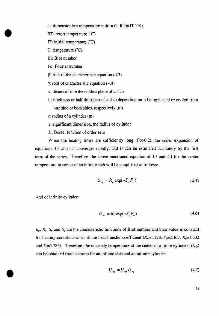
•l;: dimensionless temperature ratio =(T-Rn/(IT-TR)
RT: reton temperature (oC)
IT: initial temperature (oC)
T: temperature (oC)
Bi: Biot number
Fo: Fourier number
~: root of the characteristic equation (4.3)
y. root of characteristic equation (4.4)
x: distance from the coldest plane of a slab
L: thickness or half thickness of a slab depending on it being heated or cooled from
one side or both sides. respectively (m)
r: radius of a cylinder (m)
a: significant dimension. the radius of cylinder
ln: Bessel function of arder zero
\Vhen the heating rimes are sufficiently long (Fo>O.2t the series expansion of
equations -1..3 and -1..4 converges rapidly. and U can be estimated accurately by the tïrst
terro of the series. Therefore. the above mentioned equarion of 4.3 and 4.4 for the center
temperature in center of an infinite slab will be simpHfied as follows:
(4.5)
And of intïnite cylinder:
Rp• R. Sr and Sc are the characteristic functions of Biot number and their value is constant
for heating condition with infinite heat transfer coefficient (R,r1.273. Sp=2.467. R~-L602
and Sc=5.783t Therefore. the unsteady temperature at the center of a finite cylinder (UtJ;c)
can be obtained From soluùon for an infinite slab and an infmite cylinder:
• U"fi: =Uup .uue
(4.6)
(4.7)
62

The general equation to describe the temperature CT) as a function of rime Ct) during
• heating or cooling periods with known initial temperature (m and ambient temperature
(Rn is as follows known as the BalI equation:
log<IT - RTl) =-t1f + loge j(11T - RTl) (4.8)
Paramerers of f and j are known as the heating or cooling rate index and lag factor.
respectively. These parameters can be obtained from following equations:
j=R,,,.R,
(4.9)
(4.10)
The center temperature in a tinite cylinder was calculated through equation 4.8 to 4.10
(anal ytical solutions) and the temperature profiles from the finite difference models were
compared against the analytical solution of BalI equation. Along with the computation
time of the model.. the R.\IS of the error between the tinite difference model and analytical
solution. caIculated as below. were used as two criteria of model optimization:
where:
RiWS of
1 rt
~L{~1lOd!i. - T.uw,..ncui"
errors= ...;.,1"=...;.,1 _
n
(4.11 )
T;maiyn...~: temeprature predicted by analytical solution (oC)
Tmode= temperature predicted by finite difference model (oC)
i: each time step (Sec)
n: number of points
Five different time steps of L 5. 10 and 20 seconds and four grid sets in both of
horizontal and vertical a:ds (5&5. [0&10. 15&[5 and 20&20) were examined.
•63
•Overall accuraey evaluation of the formula metbod
A wide range of processing conditions and commercial can sizes (15 can sizes)
were emplayed as testing conditions for the finite difference program ta obrain the required
time-temperature data The finite difference model was programmed ta change the
medium temperature from heating to cooling based on a selected heating period lethality
(Ffi) in the range of 5-15 minutes. Each run of the program would provide the proeess
rime. process lethality and the temperature profile of the product at the cold point of the
cano
From each temperature profile. heating and coaling curves were separated in the
forro of logarithmic temperarure difference of the product and medium vs. proeessing time.
Determination of j and f values for heating and cooling were based on repetitive regression
to [oeaee the straight portion af heating or cooling. These values along with process time or
process lethality obtained from finite difference program were compiled in a Lotus based
program. Process lime and process lethality for selected Formula methods were calculated
using a computer program developed for this purpose (Ramaswamy. 1991). Deviations
from tinite difference model values (reference vaIues) were determined as follows:
F -F .E"or = '" 'Il' ) ,Il mllth"c;'. 1 xl00F"t,r:r J
(4.5)
•
The same method was applied to evaluate the deviations in process time
calculations. A negative percentage deviation in process Iethality demonstrates an
underes[Îmation of the lethality with the respective Formula method (and hence
undesirablet where a positive error shows inaecuraey on the conservative side. For
process time computations. on the other hand. positive errors show underestimation of
process time (and hence undesirable). while negative errors show overestimation of
methods. but on the safe side.
The accuracy evaluation of the methods was performed from two perspectives.
First.. the accuraey of methods was compared as a fonction of one parameter. while the rest
parameters had a constant value. In the second approach. the accuracy of eaeh method was
evaluated for each variable parameter over the eotire set of data.
64
•
•
Evaluation of formula methods onder specifie conditions
Accuracy evaluation of the methods was based on the g-vallie and cao sizes in fonn
of height over diameter (HID) as these were reponed eaclier as conditions under which the
methods deviate from reality (Smith and Tung. 1982). A reton temperarure of 12DoC and
initial temperarure of S013C were considered. As the tables in BalI and Stumbo methods
were based on the assumption tbat cooling water was 1OO~C below reron temperarure. the
cooling warer temperature was flXed to 20°C. The instantaneous come-up time to retort
temperature and instantaneous drop in medium temperature to the cooling water
temperature was assumed. Heat transfer coefficient of 5000 W/m~C was assumed for
steam as the heating medium and 500 W/mlC for water as the cooling medium. Thermal
conductivity of the product was constant (0.6 W/rnC) within the simulation. In order to
evaluàte the effect of g-\.'alue. the finite difference model was programmed to change the
medium tcmperature from heating to cooling based on reaching different g-values in the
range 01'0.05-15 cù•
RESTJLTS .<\l'ID DISCUSSION
Optimization of tinite difference model
The optimization results of the modeI are shown in Figure 4.1 based on the number
of nodes. both in venical and horizontal axes. as weil as time step size. Increasing the
number of nodes in each a.'(is increased the computational time due to additionaI
caicuIations ta be perfonned for center temperature prediction. Smaller increments in the
axes increase the accuracy of model in temperature prediction. aIthough as shawn in the
Figure ·t l. after an initial sharp drop from 5 nodes to la nodes. increasing the number of
nodes further had less effect. With this respect. a 10 by 10 grid size was selected as the
optimum number of nodes in both a'(es. Same trend was applied to select optimum number
of rime steps used in computation. As computation time was increasing intensely for time
step sizes less than 5 and Rl\tlS of error was not changing significantly for variation of time
steps below 5 seconds. a 5 second time step size was assigned as the optimum vaIue for this
pa.rameter in modeI.
65
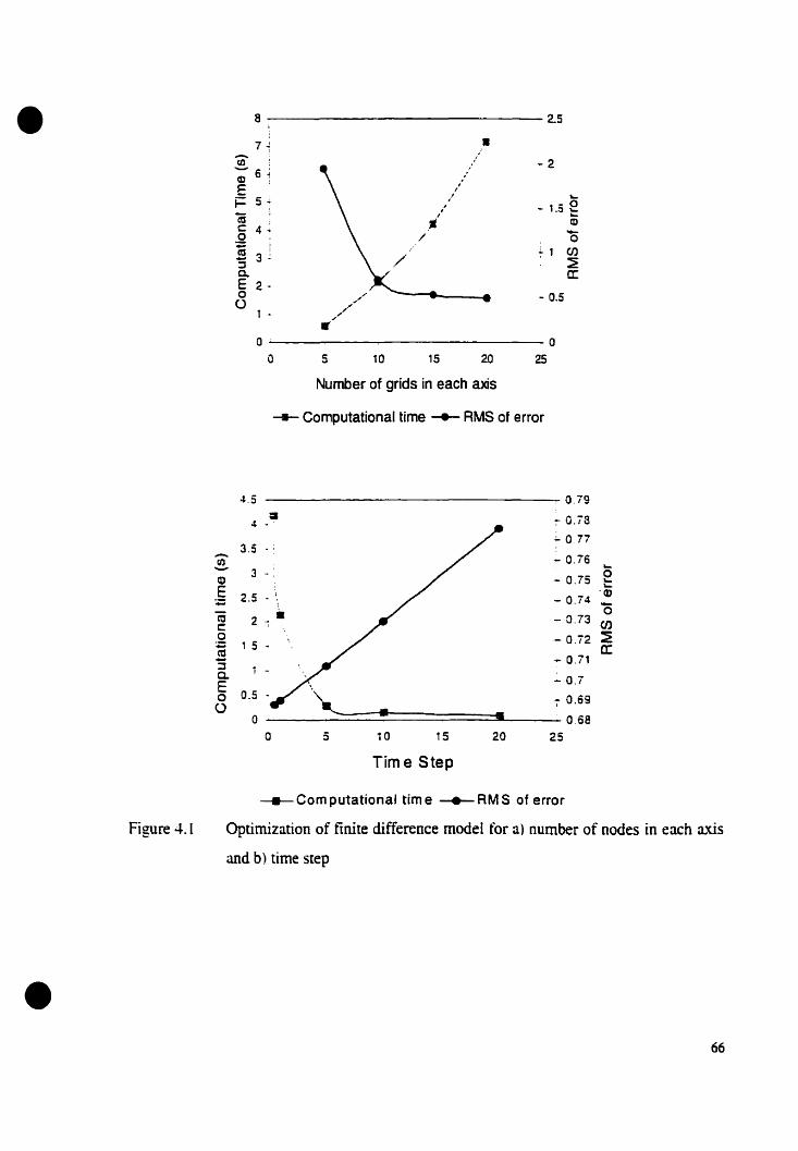
• 8 2.5
7 •ta 1
-2';6 :
E 11
i= 5 .. 11 ~
- 1.5 eëa 1
1~
! • CDc 4 1.2 / 0-; i ~ 1 Cf)
"5 3 ~ /' ~c.. CI:E 2 ~a ,// - 0.5U /1 .,",•a 0
a 5 10 15 20 25
Number of grids in each axis
-- Computational time -.- RMS of error
~.5 0.79;a
~ O.ïS4 -~ 0.77
3.5 - .- - 0.76CI)~- 3 - 0
Cl) - 0.75 ~
:§~
2.5 1
- 0.74'Q)
0(ij 2 il - 0.73c "; CIJ.2
1 5 - 0.72 ~êti - cr:'S - 0.71~
, -~ 0.7E '.
0 0.5 -~ 7 0 .69
0 • •0 0.68a 5 la 15 20 25
Time Step
•
Figure 4.1
_____ Com putational tim e --.- RM S of error
Optimization of finite difference model for a) number of nodes in each a..us
and b) time step
66

•
•
Mter optimization of the modeL the predicted temperature profiles based on finite
difference model and analytical equation were compared with each other to validate the
accuracy of the finite difference model. The result of validation is depicted in Figure 4.2 in
the farm of center temperarure profiles. The discrepancy at the beginning of the heating is
for the situation when fo<O.2 under which the two procedures were not expected to match.
However. the predicted temperatures ufter this initial deviation coincide with each other.
This should be expected as the main basis of heating equations used by each method is in
agreement \Vith the experimental data. A perfect overlapping of these two methods in this
section of time-temperarure curve demonstrate an excellent accuracy of the finÎte
difference model.
Overall evaluation of formula methods
Overall evaIuarion of selected formula methods was carried out in two directions.
First ail the considered parameters were maintained at a base condition (RT=I:!O°C.
lT=80ù C. a=1.5*IO·7m!/s and can size=303 x 509) and one pararneter at a rime was vaIied
over a selected range. Errors in process rime and process Iethality calculation were
calcuIated as relative errors (percentage deviation from reference values). Subsequently.
each parameter was'varied over the entire range with respect to ail other conditions and the
associated errors were calculated. Tables 4.1 and -t2 summarize the results of errors
associared with different models for each parameter at the base condition as weil as the
overall. [n process tinle caIculations (Table 4.1). retort temperature was the most
intluencing factor compared to product initial temperature and thermal diffusivity for a can
size 303 x. 509. Associated erroTS varied From a high -7 to -21 % for Steele & Board
method to -0.7 to -1.5% for Stumbo's method. Balrs method was close ta Steele & Board
moditïcation. while the method of Pham had errors varying from -1.5 to -8.3%. The
higher errer in process rime using the Pham method was the result of using processing
conditions and can size which resulted in high sterilization values (U(fh<O.04). below the
range of studied by Pham. Sïnce the developed process calculation equations (Pham. 1987)
were for a defined range of sterilization ratios (U/fh: 0.04-1.5). processing conditions.
which do not satisfy this range. cao result in high errors in process calculations. With
reference to initiai temperature and methods of Bail and Steele & Board
61

•140 "T""l----------------
l/ AnaJyti:aJ solution
li
40 i/
120 ~11
-1ooJo .;.-'-----t~",~ 1
~ 80 ~~ ,
- !ca~
~ 60 1EQ)
f-i,,:
20 .f
605020 30 40
TIme (min)
10
1o ~I _L... ~-----
o
Figure ·tl Validation of finite difference model against the analyticaI solution
•68
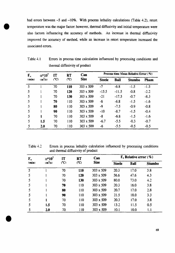
•had errors between -5 and -10%. With process lethality calculations (Table 4.2)y retort
temperature was the major factor: howevery thermal diffusivity and initial temperarure were
aIso factors influencing the accuracy of methods. An increase in thermal diffusivity
improved the accuracy of method~ while an increase in retort temperature increased the
associared errors.
Table·t 1 Errors in process time calculation intluenced by processing conditions and
thennal diffusivity of product
f u a*107 IT RT Cao Proc:ess time ~leaD Relative Enor (%)
tmint tm!/sl tOC) (oC) Sïze Steele Bali Stumbo Pham
5 1 70 110 303 x 509 -7 -6.8 -I.S -1.55 1 70 120 303 x 509 -15.5 -Il.S -0.8 -2.25 1 70 130 303 x 509 -21 -17.5 -0.7 -8.35 1 70 110 303 x 509 -8 -6.8 -1.5 -1.6
5 1 80 110 303 x S09 -9 -7.5 -0.9 -0.85 1 90 110 303 x S09 -10 -8.7 -1.5 -0.-+5 1 70 110 303 x 509 -8 -6.8 -1.5 -1.65 1.5 70 110 303 x 509 -6.7 -S.5 -0.3 -0.75 2~O 70 110 303 x S09 -6 -S.5 -O.S -0.5
Table +.2 Errors in process lethality caIculation intluenced by processing conditionsand thermal diffusivity of product
Fil a*107 IT RT Cao F0 Relative error (% )
(minI tmz/s) (OC) (oC) Size Steele Bail Stumbo
5 1 70 110 303:< 509 20.3 17.0 3.8
S 1 70 120 303 x 509 56.6 -1-7.6 4.35 l 70 130 303 x 509 80.0 73.0 -+.25 1 70 LLO 303 x 509 20.3 16.0 3.85 1 80 llO 303 x 509 20.7 17.0 2.85 1 90 liO 303 x 509 21.5 18.0 3.3
5 1 iD lIa 303:< 509 20.3 17.0 3.85 1.5 70 lIO 303:< 509 13.2 il.5 0.55 2.0 70 110 303 x 509 10.[ 10.0 l.1
•69

•
•
Compared to the process rime. the mean relative errors associated with process
lethalities were much higher because of prediction of fixed low process Iethality of 5.0
minutes (while the process rime varied from 25 to 400 minutes). Bail and Steele & Board
methods over estimated the process lethality by 17 to 80% with respect to the reton
temperature. while the error range with respect ta initial temperature and thermal
diffusivity remained at 10-20%. Stumbo·s method was fairlyaccurate with error ranges up
to ~%. Initial temperature and thermal diffusivity have been reponed ta only have
minimum effect on calculation accurney (Ghazala et aL.. 1990: Smith and Tung. 1982). In
general the relative arder with decreasing accuraey was Stumbo. Pham. BalI and Steele &
Board. [t is interesting ta note that ail mean relative eITors were negative for process time
and positive for process lethality. indicating errors generally on the eonservative side for ail
the methods.
In arder ta study the overall effeet of each parameter on process caleulation over a
broader range of processing conditions. mean and standard deviation of eITors for cach
specitïc parameter was calculated and summarized in Tables 4.3 and 4.4 for process time
and process lethality calculations. respeetively.
[n process time calculation. retort temperature and length of processing time were
more obvious parameters affecting the accuracy of methods. An increase in retort
temper.lture. increased the error terms for ail the methods. except for Stumbo·s methed.
which had the lowest error without any specifie trend in mean values. AlI methods
overestimated the process rime. as shawn by the negative sign for mean errers except for
Stumbo's method. whieh underestimated process time under sorne conditions. Sorne
~arlier researchers have observed similar results. However. it should aIso he noted that
Stumbo's method was in faet most accurate amongst the different methods. The mean
errors were less than 1% for ail situations. On an average. this accounts for a 2 minutes
error over a 100 minutes process time. obviously smalI. In comparison. BalI and Steele &
Board methods had up to 15 and 20% over estimation~ respectively. Pham's method was
close to Stumbo·s method.. with mean errors mostly in the conservative side. However. as
indicared by the aceompanying standard deviations of me mean errors (up to 2%). it is
logical to assume situations did erist for over estimation of process time. As discussed
70

•earlier. larger errars of high retort temperatures using Pham method is due ta resulted
steriliza[ion values. which were not defined by Pham (Pham.. 1987. 1990)
Table 4.3 Means and Standard Deviations (SD) of relative errors in process time
calculation for selected process calculation methods
Steele BaIl StumboParameter Range
~Iean sn }Iean sn Mean snPham
~Iean sn
-15.64 3.46
Retort
temperature
llO(ÙQ
120 (iJC)
130 (oC)
2.44
-12.93 3.66
-19AO ·"-~3
-6.20
-9.91
3.06
2.71
0.71
-0.55
lA3
0.64
1.19
-0.25
-0.35
-3.36
0.51
0.90
2.62
Initial
temperature
70 (llC)
sn (oC)
90 (üC)
-1l.3 5.25
·12A5 6.00
-14.63 7.62
-9.55 3.92
-10.57 ~.48
-12.48 5.66
OA8
0.32
-0.16
1.56
1.5S
1.85
-1.76
-1.5 1
-0.69
2.20
2.18
2.01
Thermal
diffusivity1.5*10'- tm=/sl ·11.58 6.34
!* Hr~ 1m=/st -1l.34 5.97
-11.51 5.20
-10.93 ~.97
-10.08 .t.3t
-0.21
0.24
0.61
1.34
1.65
1.93
-1.83
-1.25
-0.87
2.75
1.95
1.56
Small -11.21 5.85
Mc:diurn -[OA3 6.60Can Sïze
Urge -13 fi.51
-l.OII ~.39
-9.65 5.16
-10.38 .t.74
O...B
0.81
0.21
2.08
2.12
1.19
-1.05
-O.S7
-1.12
1.58
1.76
2.·H
-15.78 5.05 -12.71 .1.28Processing
time
Lûw
~{edium
Long
-Ll.8
-8.83
5.57
5.06
-9.34
-7.87
3.67
3.76
-0.03
0.51
0.58
1.14
1.31
2.06
-1.80
-0.79
-0..11
2.L0
2.10
l.I7
•
Based on tiU weieht: small: (<0.5 kg). ~ledium: (0.5-1 kg). Lan!e: (>1 kg): Processine..... -..... ...... """ -....,;
rime: Low: I<LOO min). Average: (100-200 min). Lang: (>200 min>
Trends observed with process lethaIity were similar (Table 4At Conditions which..
under estimated process rime. obviously over estimated the process lethality and vice versa.
With process lethality_BalI and Steele & Board methads had up ta 70% over estimation.
~lethods of Stumbo and Pham perfonned better with mean errors less than 7%.
Table 4.5 summarizes the parametric range.. mean and standard deviation of errors
for combination of parameters. The maximum error in process time caIcuIation belanged
to the method of Steele & Board with about 37% mean relative error. while methad of
Stumbo had only 5% ma'<imum mean relative error. However~ as it tS been reported
71
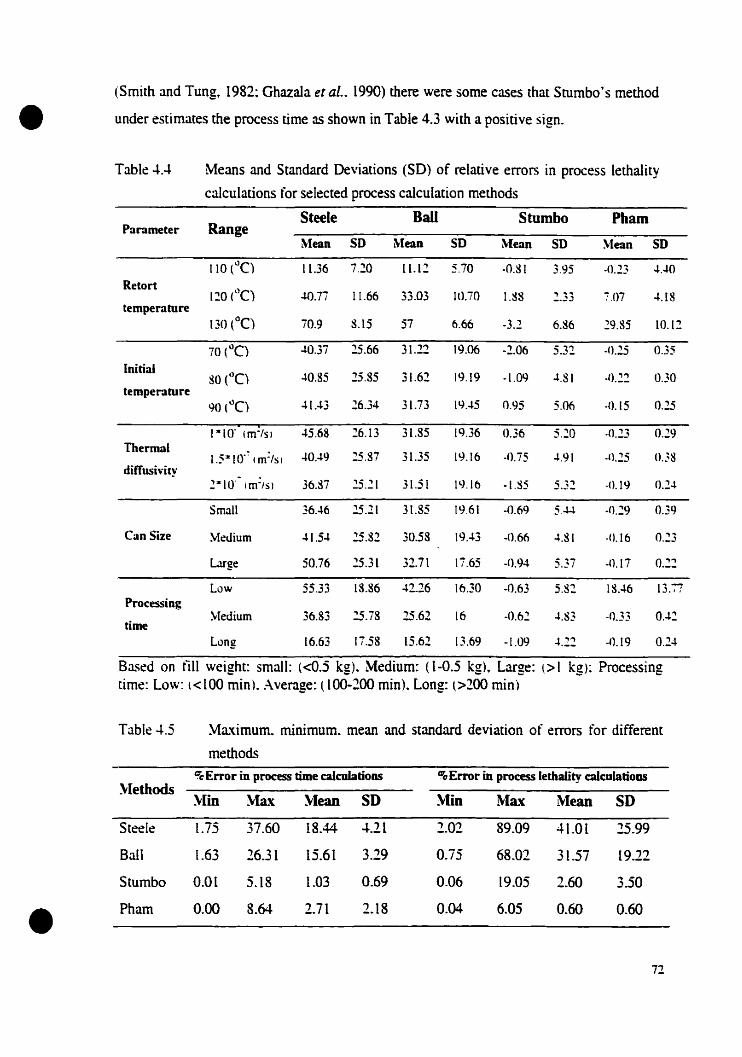
(Smith and Tung. 1982~ Ghazala et al.. 1990) there were sorne cases that Stumbo·s method
• under estimates the process tirne as shown in Table 4.3 with a positive sign.
Table ~A Means and Standard Deviations (SO) of relative errors in process lethality
calculations for selected process calculation methods
Steele Bali Stumbo PhamParameter Range
~Iean 50 ~Iean sn ~(ean SO Mean sn110 ("C) Il.36 7.20 ILL:! 5.70 ·0.81 3.95 ·0.23 ~.~o
Retort120 (ûC) ~O.7i Il.66 33.03 10.70 1.88 ., .... 7.07 ~.18_ • .).J
temperature130 (oC) 70.9 8.15 57 6.66 ·3.2 6.86 29.85 LO.12
70 (oC) ~O.3Î 25.66 31 ..22 19.06 -2.06 5.31 -0.25 0.35
Initial80 ("C) ~0.85 25.85 31.62 19.19 ·l.09 J.SI -0.22 0030
temperature90 ("C) ~tA3 26.34 31.73 lq.~5 0.95 5.06 ·0.15 0.25
,(-[O' (m-/si J5.68 26.13 31.85 19.36 0.36 5.20 ·0.23 0.29
ThermalL5:k IO'~ 1m:/sl ~O.~9 25.37 31.35 19.16 -0.75 -f..91 -0.25 0.38
diffusivity -2-10' Imïs) 36.87 25.21 31.51 19.16 -1.~5 5.32 -0.19 O.2-f.
Small 36.J6 25.21 31.85 19.61 -0.69 5...f.4 -0.29 0.39
Cao Sïze ~Iedium ~1.5~ 25.82 30.58 19A3 -0.66 ~.81 '/).16 0.23
L1rge 50.76 .;s.31 32.71 17.65 -0.94 5.37 -0.17 0.22
Law 55..33 18.86 ~2.26 16.30 ·0.63 5.81 18,46 13.77Processing
y[edium 36.83 ~.j8 25.62 16 -0.6:! J.83 ·n.33 O.~~time
Long 16.63 17.58 15.62 13.69 -(.09 J.l:! -0.19 0.24
Based on till weight: smaII: (<0.5 kg). Medium: (1-0.5 kg). Large: l> 1 kg): Processingtime: Low: t<lOO min). Average: (100-200 min). Long: l>200 min)
Table 4-.5 Ma'<imuffi. minimum. mean and standard deviation of errors for different
methods
%Error in process time caladatioDS %Error in process lethality caJculatioDS}[ethods
}[jn ~Ia.~ }Iean sn Min Ma~ ~Iean snSteele l.75 37.60 18.44 -+.21 2.02 89.09 41.01 25.99
BalI l.63 26.31 15.61 3.29 0.75 68.02 31.57 19.22
Stumbo 0.01 5.18 1.03 0.69 0.06 19.05 2.60 3.50
• Pham 0.00 8.64 2.71 2.18 0.04 6.05 0.60 0.60
72
•
•
Specifie evaluation of formola methods
Errors basecf on the can shape or HID ratio had a consistent pattern for different
Formula methads. The results are presented in [WO different fannars for comparative
purposes. First the different methods are compared at a given g-value. Then each method
is compared at different g-val[les~ In both situations HID raüo was used as the basis~
The comparison of different Formula methads at a given g-value is shawn in
Figures -1..3 and 4.4 for the process time and process lethality calculations~ respectively.
The maximum error for almost all the methods was observed for HID near to unity. Smith
and Tung (1989) and Pham (1990) observed the same trend in error patterns. Steele &
Board's method had the largest errors (-2 ta -20%) arnong evaluated methods and
Stumbo's and Pham's methods were the most accurate methods. Stumbo's method
predicted process time wirh accuracy of 1% for g-value of O.05°C and 9% for g-value of
1SoC and Pham's method had similar accuracy in process time calculation. They appeared
to deviate from each other more at g=15t)C.
Trends were similar with respect to prediction of process lethality except that the
errors were on the opposite side. Steele & Board method had the highest positive error
120-ïOce) while Stumbo's method had the least (<20% L Pham's method as suggested is
ûnly for ~stimation of process rime.. and for process lethaIity~ the method hàd to be solved
using a trail and error approach. While this approach was employed for sorne test
situations. it was not possible to extend this approach for aIl the test situations because of
the time consuming iteration process. Since methods of Pham and Stumbo were reported
be similar in most cases.. similar trends could he probably assumed for predicting the
process lethality.
With respect to sterilization values.. Lenz and Lund (1977) also considered
processes with large g-\:alues uncertain. The larger errors for processes at large g-values
are due ta accomplishment of a large part of sterilization during cooling section. In these
processing conditions. cooling time and also the product properties during cooling can be
the reason for the high errors in total sterilization value of the process~ However. for
processes with smaIler g-values~ which is more common~ the error values are small ranging
from 10% for Steele and Board~s method to 1% for Stumbo and Pham methods.
73

• a Il 0• -0.5 SIIrio
~ ·1_ ·1-. FhIm1·1.5""'= ·2
·2 1-3a: .2.5
\sz:::::.a:~
~:::wi~ t~~
~ ~ ·7~.5 ...
0 2 3 .- a 1 2 3 .-~rItiD HDratiD
c 0- ·2 Phan~
Î ~~Ia: -8t -la~~e~ ·12
·140 1 2 3 4
HOratb
42 3
HO ratio
e 0 ----........--~- .....
# ·5'ii ·10~1 ·15
;! ·20
·25 .......--------.....o4123
HO'"
·20 ---------....o
d 0 ~-------.....,
~ ·5
Îa: ·tO
t -15~
Figure 4.3 Errors in process time calculations for different g-values (a: g=O.OS C, b:g:I C: c: ~=5 CO: d: g=lO CO: e: !l=15 CO).... ... ,... ....
•74

• • 10 b 259~..8 2D ;;:.-.....-~ 7 lr 6 j'---..W l 15
5 'j'--i..f &f
f4
1103
~ 2 51
.. .A. A..su.t.o SUrDo
O. A ....... .. ~0 -0 1 2 3 4
0 1HD~ 3 4
HDr6
e ~
C~...#"35
""':30~~125
.f20f 15~ 10
SIuntlo5
.........MIJr •••00 2 3 ..
HO,.
d 70 e 1)
60~.. 70 •
lso ~fJ) ::~::::::-ÎC ~~ -19)0 ~4J ..ÂM6• .....~U.30
f20 1\... SbmIo I!J~ .... ~3J
10 10a 0
0 1 2 3 .. 0 1 2 3 4HDrd:I HO'*'
•Figure 4.4 Errors in process [ethality caIculations for different g-vaIues (a: g=O.05 CO"
b: g=L CO; c: g=5 CO; d: g=LO CO; e: g=15 CO)
15
•
•
The effect of g-value on deviations in calculation i5 a1so due to temperature
difference at the end of heating between heating medium and the product. For smaller g
vallies. when the product temperature and retort temperature at the end of heating are close
ta each other. the effect of temperature gradient i5 insignificant. However. for Iarger g
values. when this difference is Iarger. this effect can cause errors in calculation. In this
case. while the reton temperature IS changed from heating ta cooling water. there would be
a longer lag for center of the can ta receive the effect of cooling water temperature. and
even after cooling was began. the center temperature will continue increase for a short
while. ~one of the Formula methods correctly account for this effect and deviate from
reality at larger g-vaLues.
Figures 4.5 and -k6 show the performance of each formula method for at different
g-vlliues. The effect of g-vallie on each method cao be seen more clearly in this
presentation. With an increase in g-value. the associated errors for each method increased.
showing a systematic increase in crrors for methods of Bail and Steele & Board. With
respect to Stumbo and Pham methods. the errors were smalI up to a g-value of 5ù C. but
then the inaccuracy begins ta increase markedly. Again Srumba and Pham had the highest
accuracy. The deviations in process lethality and pracess rime prediction increased for HID
close to unity and for Iarger HID values the eITors decreàsed.
ï6
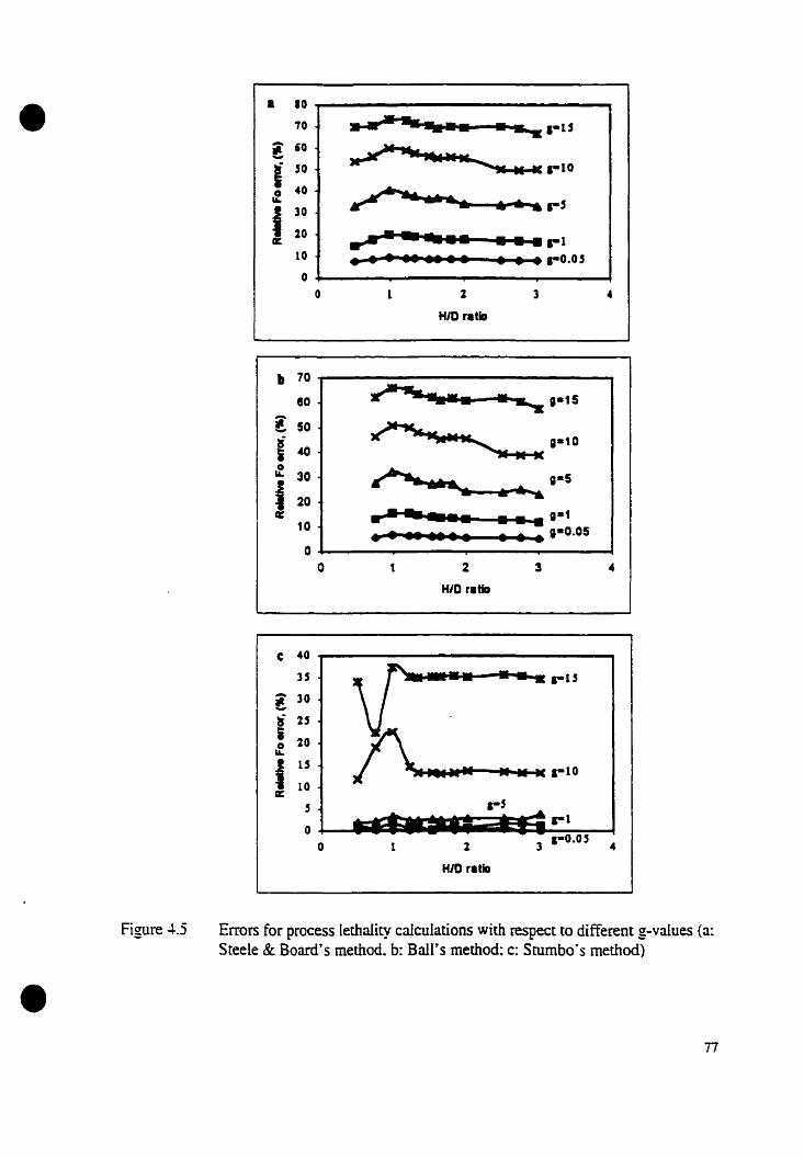
• • la70 ........... ...... 1.1'
l 60
Î '0 1-10
l 40~66,*
130 ..... r'
20 ............ -- _riCI:
la .' ....... • • • r O•O'a
0 1 2 3 4
HID ratio
b 70
80 ga15
l 50~g.tal 40
0
~..'*"- 3D gaS
1 ....20
~ w''' ••• •• • "a110 .' ...... • • • ,aO.05
00 2 3 .-
HJD ratio
C 40
3' v:--- .... ri'
- 30~
Î 2'
0 20 A.UNII.
115• If te 1-10
CI:10
5 r'rI
01-0•05
0 1 2 3 4
HJD ratla
•Figure 4.5 Errors for process lethaIity calculations with respect ta different g-values (a:
Steele & Board's method. b: Baies method: c: Stumbo~s methad)
n
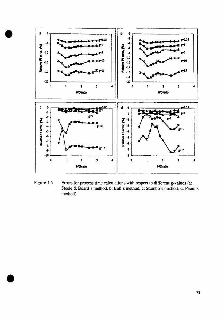
• • 0 b 0
::;:: Il MI • ••• ro·O! ·2:::::::: • ••• ,.0.05
l.,
••• r l - -4'# ~
•• .-rl••• - ~rSÎ ·10 ~,., Î ..&: &: -10
~rloI-U riO 1'12-14
cr .10 ~r15 c .16 ~ru-II
-1$ -200 1 2 3 .. 0 1 1 3 ..
IfDrIIb HOrIID
c 0rl
d 0
-1 ·1 rI·1
..,l ·3 l-Z
Î ... riO Î -]5: ·S o -4
~
i -6 ,-'-1•cr .. «~
-9rU -1
-10 ..0 2 ] .. 0 2 3 ..
HDrIdD HDrIIIID
•
Figure 4.6 Errors for process rime calculations with respect ta different g-vaIues (a:Steele & Board9 s method!' b: BaIl's method: c: Stumbo's method: d: Pham9 smethod)
78
•
•
CONCLUSIONS
The accuracy of selected formula methods was determined with respect to data
generated from a tïnite difference model. Finite difference models have the potentiaI for
accornmodating variations in processing conditions and cao size. and provide data for a
wide range of processing conditions. The optimization of the fioire difference mode1
against an analyrical solution of hear transfer equation with lOx 10 grid size predicted
accurare cemperature profiles. Process caIculation eITors were evaluated based on the
variation of each paramerer. Retort temperature was one of the most major parameters
intluencing the accuracy of the selected process calculation methods. NIost methods
overestimated the process rime with the exception of Stumbo's method for sorne cases of
underestimation. Based on the cao shapes. errors had an increase for HID values near [0
unity. Errors increased at larger g-values. where a substantial amount of process
sterilization is accomplished during the early cooling stage. This trend in errors was
observed for aIl the methods. Stumbo·s methad was considered the mast accurate method.
following it was Pham's method.
79

•
•
CHAPTER5
ARTIFICIAL NEURAL NETWORK MODELS AS ALTERNATIVES TO
THERi'lAL PROCESS CALCULATION ~IETHODS
ABSTRACT
Artificial Neural Network (ANN) is a computing system capable of
processing information by its dynamic state response to extemaIinputs.Al.JNs
learn from examples through iteration by adjusting the internaI structure ta
match the pattern between input and output. In this study, finite difference
simulations, which are widely recognized as' practical alternatives to
experimental methods, were used ta generate temperature profiles for a wide
range of can sizes under variaus pracessing conditions. The time-temperature
data were used ta compute the process lethality, process time as weIl as heat
penetration parameters: 1:, ilt, t: and jer:. These data were used for developing
the Al\fN models (bath training and testing). The accuracy and ability of ANN
models were compared with selected Formula methods, bath with respect ta
process time and process Iethality computations. Process calculation results
from ..~\fN model were comparable to Pham's and Stumbo·s methods, which
\vere previously evaluated as the most accurate amongst the process
calculation methods.
80
•
•
INTRODUCTION
Artitïcial Neural Networks (ANNs) have been the focus of interest in many diverse
tields of science and technology. Neural networks are basically computer models. which
simulate very simple abilities of our brain. Rather than being programmed for use in a
particular application, neural network models generate their own mIes by leaming from
provided examples. Al.'IN has the ability of approximating arbitrary continuous functions
based on a set of given observations. As they obtain this ability through the stage of
learning. they are known as truly adaptive systems, which do not need any prior knowledge
of the nature of relationships between the set of parameters. A.1'lN models are thought to be
robust to noise and inconsistencies in data. rendering them more advantageous compared to
empirical models. Also. AJ.'1N models can be multiple-input and multiple-out (~IThIO)
systems fBaughman and Liu, 1995). Therefore, variability of multiple parameters in the
development of an AJ.\fN model is possible. NeuralWare (1995) provides a wide overview
of potential applications of neural network as classitïcation. prediction. data association
and optimization. Most food related work involves estimation. prediction and control
(Eerikainen et al.. (993).
\Vîrh respect to ANN characteristics and their abilities in modeling. their
application has been considered in the development of a general model in thermal process
caIculations. Accurate detennination of thermal processes is required \Vith respect ta
assurance of safety. as weil as retention of quality attributes and nutritional values of food
products. For this purpose. different methods have been developed for facilitating thermal
process calculations. AIl these different methods are aimed at determining the lethality
(F,,) for a given process or calculating the process time for achieving a given process
lethality. [n arder ta establish thermal processes.. time..temperarure data of the product
undergoing the thermal processes is required. ~[ore versatile. less expensive and less rime
consuming alternative of experimental procedures are mathematical models.
Finite difference models of heat transfer inco packaged food have been successfully
applied in optimization and control (Teixeira et al. a. b~ 1969: Dana et aL, 1986: Teixeira
and Manson. 1982: Tucker. 1991: Teixeira and Tucker. (997). The main feature of these
models is the prediction of temperature profùe based on the goveming heat rransfer
81
•
•
equations of packaged food products. Fmite difference rnodels require sorne specification
of the food product and system such as thermal diffusivity of the food product.. heat transfer
coefficient of the heating or cooling medium and thermal conductivity of package. When
these conditions are known.. the time-temperature data can he obtained at any specitic point
of the packaged food product for any processing condition and package sizes. The ease of
use of tinite difference model can he considered in providing an expanded data set.
including a wide range of parameters.
In Chapter 3. the patentia! of Al'IN to simulate two of the rnost widely used process
calculation rnethods was demonstrated. In Chapter 4. the prediction errors associated with
the available process caIculation methods were evaluated using those computed from a
tïnite difference numerical model as reference. Ir was shawn that the prediction errors vary
depending on the processing conditions. and hy far Stumbo and Pharn·s method are the
most aCCUïJ.te. In Chapter 4. a basis was aIso established for generating parametric vaIues
~uch asJh.j~.jc-L· andi:h for various operating conditions involving different retort and initial
product temperature. thermal diffusivity of the product and can size as well as the
associated process time and lethality. This provides a wide range of input-output
parameters for establishing and/or verifying useful process calculation modeIs such as chey
are airned in the present research-an A1'J~ based process calculation mode!.
Hence. the specitïc objective of mis chapter was to develop an AJ.'lN model as an
alternative to existing thermal process calculation methods using the wide range of data set
obtained from the appropriate finite difference models and initial conditions.
~lATERIAL A1~ ~IETHODS
Data generation
ln arder to obtain the training data set for Al'lN models development. a wide range
of processing conditions. product characteristics and packaging sizes were considered as
detailed in Chapter 4 and summarized in Table 5.1. The defined range of each parameter
covered the cornmon range of processing conditions. and different cao sizes were selected
from those used in industry. A fmite difference program wrinen in Fortran language
82

•(Sablani. 1995) was applied ta obtain the related time-temperature profile ta each set to
conditions. This model was based on the conduction heut transfer for cylindrical packaged
food products. The heat transfer coefficient of heating medium (steam) and cooling
medium (wacer) were assumed ta be 5000 (W/m2C) and 500 (W/m2C).. respectively. Each
combination of detïned values was applied as the initial inputs of finite difference model to
obtain the respective temperature profiles.
Each time-temperarure profile was divided into two semi-Iogarithmic curves of
heating and cooling. In order ta locate the beginning of straight Hne in each curve an
Iterative regression technique was applied andfh,!ctjn: andjch were obtained for each set of
condition. Hence a data set was obtained which.. consisted of processing condition (initial
remperature. reton temperature). can size (height and diameter). product characteristic
(thermal diffusivity). process time. process lethaliry and respective heating and cooling
parameters. This data set with 1215 data records was considered as the basis for A1'iN
models training.
Table 5.l Range of parameters used in finire difference program
Retort Temp.. l Initial Temp. Thermal diffusivity Heatiog lethaHty(oC) (oC) *I01(m2/S1 (min)110 70 1.0 5.0120 80 1.5 10.0130 90 2.0 15.0
Cao size no. 1
Cao size , Approximate fill wt. (kg) Radius*Hieghtl2(cm)
'6z 0.170 2.70:< ~.50, : 8 z taIl 0.240 3A·l :<~.13.... ; ~o.l picnic 0.300 3..1.1 :< 5.08~
~ : No.211 cylinder 0.370 3.41 :<6.195 ' No. 300 0.410 3.81 :< 5.046 No.l taH 0.454 3.89 :< 5.957 ' ~o.303 0.454 4.05 :< 5.56S ~o.303 cylinder 0.595 4.05 x 7.079 ~o.l vacuum 0.340 4.]6 x 4.2910 : No.l 0.568 4.36 x 5.80II ~o.2 cylinder 0.738 4.36:< 7.3012 No.2 ~/2 0.822 5.16 :< 5.9513 No.] cylinder 1.420 5.40:< 8.891~ No.5 1.645 6.51 x 7.1515 No. 10 3.000 7.86:< 8.89
•83

•
•
A.J.~N model development
A precise ANN model training requires selection of independent input variables
(Baughman and Liu. 1995). If a prior relation between input variables in not available. one
of the proposed methods to select the independent variables between input variables. is to
discard one variable and train the Ai'lN mode1 based on the remained set of data.
Obviously. discarding variables. which are function of the other. will not affect the
training. However. when a science of relation between variables is provided. this
information should be applied to reduce the number of input variables and increase the
accuracy of A.l~~ modeI. Based on the infonnation obrained. while developing Al\iN
model for methods of BaIl and Stumbo. the key variables for relating process time (g
value) and process lethality (f,/U) were considered as the major inputs. As the variation of
j({' values is oot integrated. therefore jn: was considered as another independenr input for
each model.
Input variables (g-l/alue or f,/U) were calculated based on the procedure applied in
the Bail method (Figure 5.1). Accordingly. the combination of these variables is used in
forro of log g or fi/V. alang with variability of jl"C related the process time [0 process
lethality or vise versa. The procedures of .~\i'N model development were followed much
closely [0 the A.l\l'N model development of Stumbo's method. The data set was divided [0
training subset and testing subset to be used during the training procedure.
NeuralWorks Professional IIIPlus. version 5.23 (NeuralWare Inc.. Pittsburgh. PA)
was employed for ~\fN modeling. A standard backpropagation algorithm with Tangent
hyperbolic transfer function and normalized cumulative delta leaming mie were seIected
for .-\..\rN models training. Same fonnats of input and output variables as detailed in the
Stumbo .-\l\i"N model were applied. For predicting the process time.JiIU were used as well
as jn [0 predict g-value and subsequently. for predicting the process lethality. g-value and
j,x were used to predictlj/U. The predicted parameters from ANN models were applied to
calculated the respective process rime and process lethality. For convenience !vIodel A and
Madel B were used to name each model for process rime and process lethality prediction.
respective1y.
84
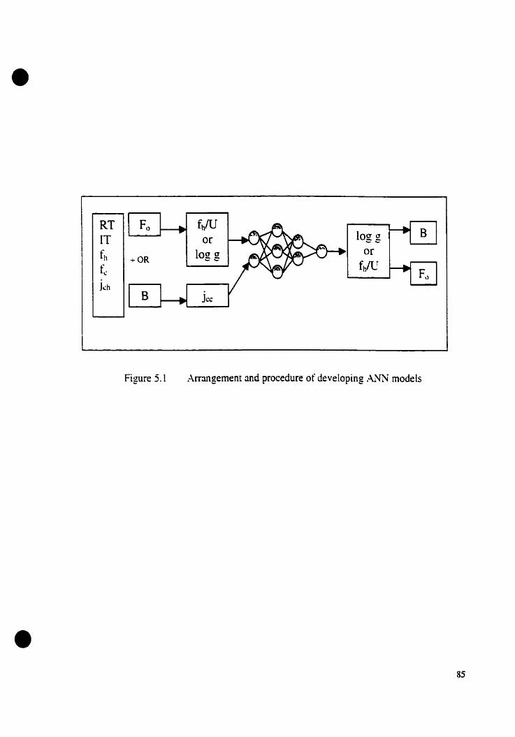
•
RT fh/U100' crIT or ee
fh 100' cr or+OR ee
fhlli(
J~h
Figure 5.1 Arrangement and procedure of developing .-\l'IN models
•85

• Optimization of ANN models
The ANN models were optimized for the number of data records in training set.
number of processing elements~ momentum vaIue and epoch size. The assigned values for
each of these parameters are summarized in Tables 5.1 and 5.3. The first step was to select
the optimum number of data in training set with respect ta default values of network
architecture. The selected training set sizes were applied to choose the optimum topology
of the networks. Afterwards. two learning pararneters. momentum and epoch. were tested.
The following criteria were used for evaluating Ai'IN models performance:
~ (Yo -Y):Roat ~lean Square (R1\1S) of error= L n
~Iean Absolute Error (~IAE) =~[ean of 1Y" - YI
Ir -yiylean Relative Error (YIRE. %) =Nlean of . Il *100
Ya
where:YI): Desired value
Y: fu~'N predicted value
n: number of records
Table 5.2 Combinations of training and testing data for network optimization
•
Group(s) inTraining set
.-\
.-\.f
.\. C. F
.-\. B. C. F
.-\.B.C.O.F
Group(s) inTesting set
B.C.D.E.FB.C.D.E
B.D.. EO.E
E
Number of datapairs in Training
set
202
.J04
606
808
1010
~umber of datapairs in Testing
set
1010
404
606
808
202
86

•Table 5.3 Range of network architecture and leaming parameters used in the study
Number of Pes~(omentum Epoch
1 hidden layer ! 2 hidden layers1.,i 2&2 0.2 4
5 1 2&5 l 0.3 81
10 5&51
0.4 16
L5 10&51
0.6 20
!1 0.8 321
• 80ld numbers wirh underscore are default values provided in software.
Comparison of ANN models
The predicted k'iN values of process time and process Iethality were compared
with respective values of the selected fonnula methods. The same methodology as the one
used in comparison of formula methods was applied to compare the performance of the
developed .-\l'IN models. Ail the predicted values from either ANN mode1 or formula
methods were compared against the reference modeL which \Vas the data from tinite
difference modeL Relative error computed as follows. was applied as the error parameter:
F -FError = .Ilrrr 1 o/tnétNIJ.JJ .rlOO
F.'I~! l
(5. L)
•
This error panlmeter was calculated based on lethality and rherefore a positive error
of Iethality calculation demonstrates an underestimation. while a negative sign shows an
overestimation of process rime. The error signs for under and overestimation are reversed.
while predicting the process rime.
RESULTS A1~ DISCUSSIONS
A1~ models optimization
Figures 5.2 and 5.3 shows the required number of data for ~Iodel ..~ and Model B~
respectively. In Model A. the performance of the network was not a function of training
set size. and a training set with 808 data (50%) was selected. However. Madel B was more
Si

• O.t
0.09
0.08
O.Oï
0.06
<'( 0.05:;;
0.04
0.03
I).O~
0.01
l)
~O~ .w4 606 SOS 1010
:"lumber or ~xarnples ID tr.umng sel
.Tr.ùrnng DTesllng .Tesung W!1050
Figure 5.2 Leaming curve for .-\!~N model A.
I}.O"
I}O~5
no~
Il 0:5
-( Il.0!~
Il III ~
IlOI
tlO05
n::0:: J04- 606 SOS IOIO
~umber of examples ln tralDlng set
.Tr:uning Cl Tc:stmg .T~stingW/I050
•
Figure 5.3 Leaming curve for .o\1\i~ model B
88

•
•
dependent on the training set size, and a data set with LOlO dat~ which had the lowest errer
of prediction was used. Although the source of data for both models was same. the nature
of variables affected the performance of the network and the question how weB network
can lcarn depended on the input variable.
Figure 5.4 depicts the effect of PEs and number of hidden layers for ~Iodel A and
B. In bath models. 2 hidden layer networks had a significanùy higher performance
(Baughman and Liu. 1995: Swingler. 1996). A network with 2 and 5 PEs in each hidden
layer had the highest performance for Madel A and 2 PEs in each hidden layer for ~lodel
B. which \vere selected as the optimum topology. Table 5.4 shows the result of learning
paramerers variations for bath models. The effects of momentum and epoch were not
signitïcant for ~lodel A and increasing momentum increased the error. A momentum value
of 0.4 and epoch size of 4 was selected for ~todel A. The effect of rhese parameters was
even Iess significant for ~lodel B. Therefore. the default value of momentum and epoch of
4 were selected.
Table 5A Effect of momentum and epoch size on the pelformance of ~lodel A and B
~IRE MRE~Iomentum . Epoch
Jfodel.-\ .\lfodeL B .'IIodeL.-\ .Hodel B
0.2 0.039 0.029 4 0.035 0.028
0.3 0.039 0.029 8 0.037 0.028
OA 0.041 0.029 16 0.041 0.029
0.6 0.049 0.019 20 0.043 0.029
0.8 0.116 0.030 .. .., 0.053 0.030~-
Performance of the ANN models
The performance of ANN models A and 8 are ShO\\l1 in Figure 5.5 as plots of Al'lN
predicted values vs. reference values from the finite difference simulation. The predicted
values for bath models were very close to desired vaIues and were evenly distributed
throughout the entire range. The associated error parameters are summarized in Table 5.5.
High R: values shows the excellent perfonnance of bath Al.'lN models in predicùng the
output variables.
89
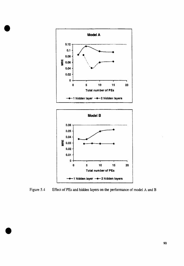
• ModelA
0.12
0..1 0---0.08 \w •i 0..06 " ~
0..04 "'.-/0.02
0
0 S 10 lS 20
Total number of PEs
-.-1 hidden layer -.-2 hidden layers
Model B
0.06--------~-----
0.05
0.04
20
•
15
•
105
..- .wi 0.03
0.02
0.01
O+---~--~--......,.....--~
oTotal numberof PEs
-'-1 hidden layer -e-2 hidden [ayers
Figure 5A Effect of PEs and hidden layers on the performance of modeL A and B
•90
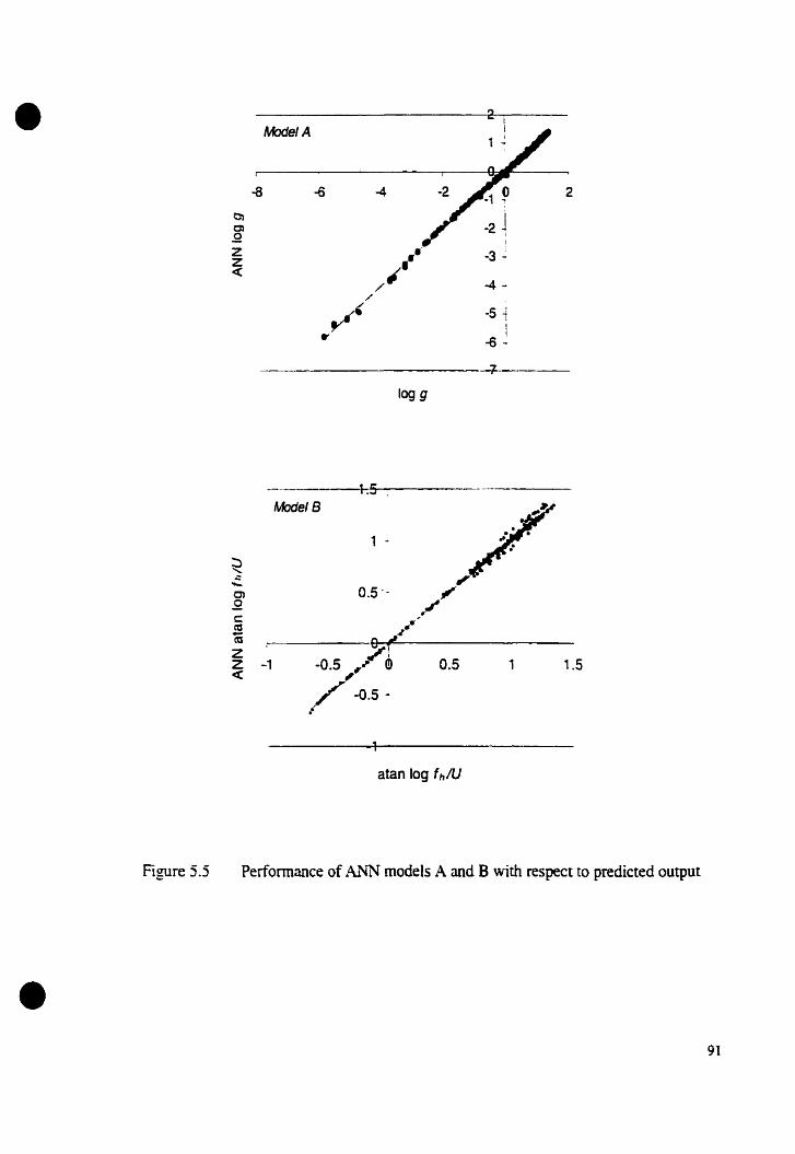
• 2ModelA
-8 -6 -4 2
0)
0.QZ •• -3 ~z
~.<{
/ -4-/
1
~'-5 ..1
-6J...7
logg
1.5 ,
~..::Cl)
.2c::ca(;
ZZ -1oC(
•
Figure 5.5
atan log fh/U
Perfonnance of ANN models A and B with respect to predicted output
91

•The performance of Al\fN models is shown in Figure 5.6 in forrn of process time
and process lethality calculated from ANN predicted g-value or f,/U vs. me process time
and process lethality obtained from the finite difference model. Both ANN rnodels showed
a good perfonnance for predicting process rime and process lethality. The error parameters
of Al~N models prediction are 5ummarized in Table 5.5. Both models had a high R2 close
ta unity showing excellent correlation between A1~ predicted values and reference values.
R~[S of crrors for proce5s time prediction was higher than process lethality since process
time had higher values compare ta process lethality. however close mean relative crrors of
bath models shows close performance of models. Hawever. with respect to process
lethality mean relative error i5 more imponant error parameter and provides better
evaluation. [n process time calculation. mean average error of 2.7 minutes indicated high
accuracy of ANN model in process time prediction applied range of this pararneter
1between -1-0-450 minutes)
Table 5.5 Errar parameters for performance and veritïcation of AJ.'IN models A and B
•
ANN~[odel A :\NN ~Iodel 8Error parameters
logg Process lime Alan log/ilL" Process lethality
R1\(S 0.05 .+.17 0.02 nA!
MAE 0.03 l.70 0.01 0.27
MRE ~.93 2.1.+ .+.~ l.7"R; 0.998 0.997 0.997 0.999
Comparison of Al'iN models with existing fonnula methods
The performance of Al~~ models were compared for range of processing
conditions. thermal diffusivity of product. can size and processing lime with the
performance of three selected Formula methods of Bail. Stumbo and Pham. The
performance of each method is showed based on the mean of relative errors and standard
deviation of error for both process rime and proces5 lethality (Tables 5.6 and 5.7).
Althaugh no particular trend was observed in mean and SO of errors based on Al'IN
models. the performance of A1'IN models was fairly in range of methods of Stumbo and
Pham.. if not better. It shauld he mentioned these two methods have the highest accuracy of
92
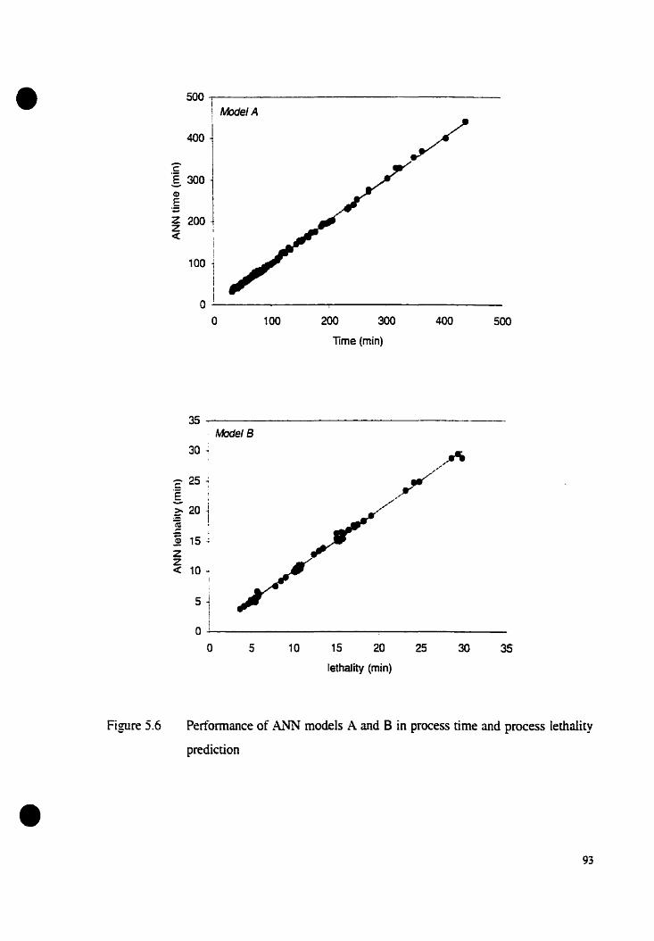
• 500 j
l ModelA
400 1 /l~ 1
; 300 i
~ 200 j<{ :
1
!100 11
1
1
1
Q'
a 100 200 300 400 500
lime (min)
35-----------------~-
35302515 20
lethality (min)
105
5 11
a .....1------------------o
. Madel B
30 ~
ê 25 ~
'Ë :;: 20 t
=: 1tU !~ 1
j 15 ~zz<{ 10 ~
1
Figure 5.6 Performance of A1\lN models ..1\ and B in process tirne and process lethality
prediction
•93
•
•
calculations compared ta other formula methods (Smith and Tung. 1982: Pham. 1990~
Stoforos. et al.. 1997).
The general performance of the selected formula methods and the Al'IN models are
compared in Figures 5.7 and 5.8. BalI method. for considering the restrictive assumptions.
had the most deviation while other methods have a close perfonnance (R~.99). The
same trend was applied while comparing the performance of other methods and ANN
models with respect to process Iethality calcuIations. As the tinite difference program was
run based on a. pre-assigned heating lethality. the process lethality is clustered around three
tïxed lethality values (one of the reasons for higher errors).
Table 5.8 shows the range of errors for process time and process lethality for
formula methods and A1\fN models. The range of errors as weil as the mean and SD of
A~\jN model for process lime prediction was in range of Pham's method. Also. in process
Iethalitv prediction the range of errors varied between Stumbo's method and Pham"s
method. The range of errors in process lethality calculations was very close to Pham·s
method and the same trend in range of errors applied for process time calculations.
94
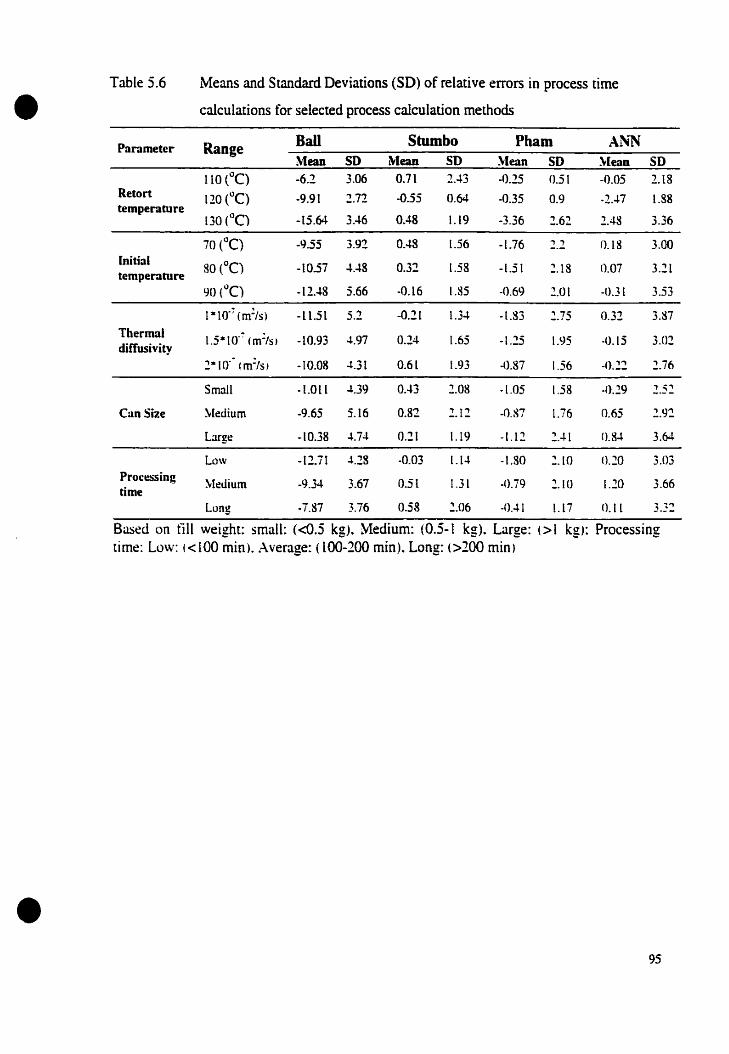
Table 5.6 Means and Standard Deviations (SD) of relative errors in process time
• calculations for selected process calculation methods
Parameter RangeBaU Stumbo Pham A1"~~Iean SD ~Iean SD Mean 5D ~[eaD SO
1[Q ('JC) -6.2 3.06 0.71 2A3 -0.25 0.51 -0.05 2.18Retort 120 (oC) -9.91 2.72 -0.55 0.64 -0.35 0.9 -2A7 1.88temperature
[30 (oC) 0.48-15.64 3.46 1.19 -3.36 2.62 2.48 3.36
70 (oC) -9.55 3.92 OA8 1.56 -1.76 ' ., 0.18 3.00Initial 80 (oC) -10.57 ~.4S 0.32 1.58 -1.51 2.18 0.07 3.21temperature
90 (oC) -12.48 5.66 -0.16 1.85 -0.69 2.01 -0.31 3.53
1'1110.7(mZ/s) -11.51 5.2 -0.21 1.34- -1.83 2.75 0.32 3.87
Thermal 1.5* [Q-~ (m:/s) -10.93 ~.97 0.24 1.65 -1.5 1.95 -0.15 3.02diffusivity
2*1O'-lmz/S) -lO.08 4.31 0.61 1.93 -0.87 1.56 -0.22 2.76
SmalL -1.011 4.39 0.43 2.08 -L.05 1.58 -0.29 2.52
Can Size ~(edium -9.65 5.16 0.82 2.12 ·oJn l.76 0.65 2.9~
Large -10.38 ....74 0.21 1.19 -1.12 2Al n.S4 3.64
Law -12.71 J..28 ·0.03 1.1... -1.80 2.10 0.20 3.03Processing
~Iedium -9.34 3.67 0.51 1.31 -0.79 2.10 1.20 3.66rime
Long -7.87 3.76 058 2.06 -OAI l.17 0.11 3.3~
Based on till weight: small: «0.5 kg). ~ledium: (0.5-1 kg). Large: (>1 kg): Processingrime: Low: 1<100 min). Average: (100-200 min). Long: (>200 min)
•95
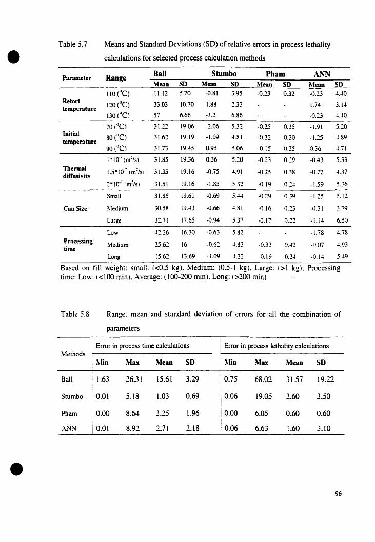
Table 5.7 l\'[eans and Standard Deviations (SO) of relative errors in process lethality
• calculations for selected process calculation methods
Parameter Range Ball Stumbo Pham A1~
~Iean SD Mean sn ~Iean sn ~leaD SO110 (oC) 11.12 5.70 -0.81 3.95 -0.23 0.32 -0.23 4.40
Retort120 (oC) 33.03 10.70 1.88 2.33 1.74 3.14
temperature130 (oC) 57 6.66 -3.2 6.86 -0.23 4AO
70 (ùC) 31.12 19.06 -2.06 5.32 -0.25 0.35 -1.91 5.20Initial 80 (oC) 31.62 19.19 -1.09 4.81 -O.~ 0.30 -1.25 4.89temperature
90 (')e) 31.73 19A5 0.95 5.06 -0.15 0.25 0.36 4.71
l''IO·~ (m:/s) 31.85 19.36 0.36 5.20 -0.23 0.29 ·OA3 5.33
Thermal l.5*10·-:- (m:/sl 31.35 19.16 -0.75 4.91 -0.25 0.38 -0.72 4.37diffusivity
2* 10'-:- (m:'s 1 31.51 19.16 -1.85 5.32 -0.19 0.24 -1.59 5.36
Small 31.85 19.61 -0.69 5.44 -O.~9 0.39 -1.25 5.12
Cao Size Medium 30.58 19.43 -0.66 4.81 -0.16 (l.23 -0.31 3.79
Large 32.71 17.65 ·0.94 5.37 -0.17 0.22 -1.14 6.50
Low 42.26 16.30 ·0.63 5.82 -1.78 4.78
Processiog Medium 25.62 16 -0.62 -1..83 -0.33 OA2 ·0.07 4.Y}lime
Long 15.62 13.69 -1.09 4.22 -0.19 0.24 ·0.14 5.49
Based on tïll weight: smaJI: «0.5 kg). ~[edium: (0.5-1 kg). Large: (> 1 kg): Processingtime: Law: «100 min). Average: (100-200 min). Long: f>200 min)
•
Table 5.8 Range. mean and standard deviation of errors for aIl the combination of
parameters
1
Error in process time caIculations i Error in process lethality calculations~[ethods
, ~lin ~[a.'~ ~(ean SD ! ~lin ~[a.~ ~Iean snl
Bali : 1.63 16.31 15.61 3.29 : 0.75 68.02 31.57 19.12
Stumbo 0.01 5.18 1.03 0.691
0.06 19.05 2.60 3.50
Pham 0.00 8.64- 3.25 1.96 6.05 0.60 0.601 0.00
i 0.01 8.92 2.71 2.18 1
6.63 1.60 3.10A.L\fN : 0.06
96

• 500500
450 0 450 • 0
400 400·
ê 350 "2 350 .
"Ë 300 ~ §. 300 •- ' a:: 250 ;â: 25Q ~
Z 200 ~ ~ 200·Z ~
< 150 ~ a.. 150 ~:
100 • 100 •
~: 0.998!
R2: 0.99950 . 5010 0
0 200 400 600 0 200 400 600
Ref. Pt (min) Ret. Pt (min)
o
400 600200
100 .
600 ~,-----------
500 ~;1
'2 400 \
lâ: 300·
aiCD 200 ~
400 600200
500 ------------
-150 .
~OO ~
:s 350 .E- 300 .
â: 250.o"ê 200·
.2 150CI)
100 .
50 .
0-----------o
Ref. Pt (min) Ref. Pt (min)
Figure 5.7 Performance of A1\fN model in process time calculation in comparison with
the other selected Formula methods
•97
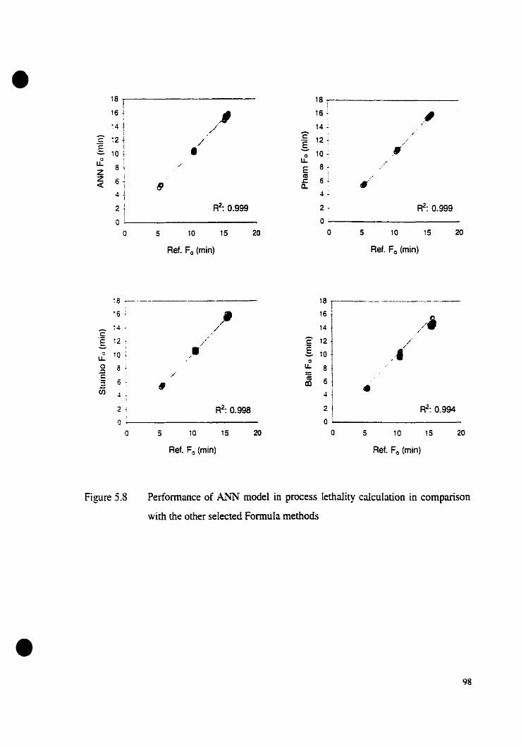
• 1a 18
16~
16 ,14 / 14
;
C ;
c 12 / §. 12E 10 • 0 10 ~
,0 U- ,
U- a ,-~ B -
Z c: ;
Z m 6 j -'
6 = .'« 9 CL4 ~ ~
2 R2: 0.999 2 ~ R2: 0.999
a 0
a 5 la 15 20 0 5 TO 15 20
Ref. F0 (min) Ret. F0 (min)
~8 ~-- 18 1~6 ;
~T6 1
/i14 . T4ê' ./
/g 12 ~ / ê 12 /1 • §.u: 10 ~ / 10 /-10
0 8 ; U- a~
/ (ij6 : • CD 6
éii 4 1 •..1 •, 12 '* R2: 0.998 21 ~: 0.994a o '
a 5 TO 15 20 a 5 10 T5 20
Ret. Fa (min) Ref. Fa (min)
•
Figure 5.8 Performance of Ai'IN model in process Iethality calculation in comparison
with the other selected Formula methocis
98
•
•
CONCLUSIONS
With respect to preliminary results from ANN modeling of BalI and Stumbo's
method. the possibility of Al'fN model deveIopment as an alternative to existent methods of
thermal process caIcuIations was studied. A finite difference modeI was applied to obtain a
wide range of data covering the applicable range of processing conditions and can sizes.
Considering the accuracy of Al\JN based Sturnbo's modeI. the same procedure of A.:.~
model development was applied. ANN Madel A with 50% data from the total data set. had
the best training error. while the M'IN ~[odel B required higher number of examples in
training 11010 data). Both models had 2 hidden layers. ~[odel A with 2 and 5 PEs in each
layer and ~(odel B with 2 PEs in each hidden layer. The initial data was transfonned to
comply with Stumbo's table and relating of process time and process lethality was
perfonned through g (or fil'}) andi:t: to fr/Cf (or g). Using Al.'lN predicted values. process
rime or process lerhality was calculated. Al'IN Model A with 2.70 minutes ~IAE was
comparable with Pham method in process time prediction. AIso. the ANN ~[odel B
predicted the process lethaIity with 2.74% of relative error. which was very close ta
Stumbo's method. As the methods of Pham and Srumbo were assigned as the most
accurate methods of process calculations. the Al'lN models had the· patential of application
in process calculation methods.
99

•
•
l.
,
CHAPTER6
GEl~ERALCONCLUSIONS
The first phase of the research was development of ANN based on Bali and Stumbo
methods~ which are the [WO major and most widely used methods of thermal
process calculations. This work was carried out ta evaluate the potentiaI for the
application of A.:.\TN technique for process calculations. A well-trained network
required appropriare number of training data set. optimized number of processing
c:lements and hidden layers and internai parameters of the network. For validating
rhese A.'IN models for each method. a new set of processing conditions were used..
and the ANN predicted values were compared to correspondent values from
method. A~~N models had 1% error in both process time and process lethality
prediction based on Bali table data and 3% error for Stumbo table data. The higher
error of Stumbo method could be possibly because of the limited number of data
and extended range of variables in A1~'N model development. However. a close ta
unüy value for R: showed good patential of .'-\l'lN technique in thermal process
l:alculario.ns.
The accuracy of selected formula methods (Steele and Board. BaIl. Stumbo and
Pham) were evaJuated for a wide range of processing conditions~ product thermal
diffusivity and cao sizes. A finite difference simulation was used to provide the
reference values of process rime and process calculations as weil as the heat
penetration parameters (fh ! jetb t~ and jcc). The performance of the finite difference
model was optimized and verified against the analytical solution of conduction heat
transfer equarion. Retorr temperature was the mast significant parameter on the
performance of methods. Methods of Stumbo and Pham had the higher accuracy as
compare to the IWO other methods. AIso in a more specifie evaluation. the methods
were compared based on the cao shapes and g-values. For dimension of HID close
[0 unity the errors were highest and they farmer increased with g-vailles.
[00
•
•
As the final goal of this study? Ai'lN models were developed as the alternatives to
present process calculation methods. The dara from the Hnite difference simulation
was applied to develop A1'lN models. Training set size was selected based on a
developed a learning curve. Using [wo hidden layers for networks significandy
increased the perfonnance of the A1'iN models: however. learning parameters were
less meaningful during development of models. A1\fN models had ex.cellent abiliry
in process rime and process lethality prediction with 2.7 minutes of mean relative
errors for process time prediction and 0.27 minutes of mean average error for
process (ethality prediction. The accuracy of Al'iN model was compared to
perfonnance of existing fonnula methods and mey closely performed to methods of
Stumbo and Pham.
101
•
•
REFERE1~CES
Angerosa. F.. Giacinto. L.D.~ Vito. R.• and Cumitini~ S. 1996. Sensory evaluation of virginolive oil by artificial neural network processing of dynamic head-space gaschromatographie data. Journal of the Science of Food and Agriculture 72:323-328.
BalI. C.O. 1923. Thermal Process Time for Canned Food. Bull. 7-l< 37) Nad. Res. Concil.\Vashington. D.C.
BaIl. C.O.. and Oison. F.C.W. 1957. Sterilization in Food Teehnology-Theory. Practice andCakulation. ~lcGrow Hill. New York.
Baughman. D. R.. and Liu Y. A. 1995. Neural networks in bioprocessing and chemical~ngineering. Academie press. Ine. San Diego. Califomia.
Bigelow. \V.C.. Bohan. G.S.. Richardson. A.C.• and Bali. C.Q. 1920. Hear penetration inprocessing canned foocis. National Canners Association. Bull 16L.
Bachereau. L.. Bourgine. P.. and PaIagos. B. 1992. A method for prediction by combiningdata anal ysis and neural networks: application [0 prediction of apple quality using nearinfrared spectra. Journal of Agricultural Engineering and Researeh 51 :207-216.
Briandet. R.. Kemsley. E.K.. and Wilson. R.H. 1996. Approached to adulteration detectionin instant coffees using infrared spectroscopy and chemometrics. Journal of theSdence of Food and Agriculture 17:359-366.
Carslaw. H. 5.. and Jaeger. J. C. 1986. Conduction of heut in soHels. 2nd Edition. OxfordCniversity Press. C.K.
Casso G.V. 1947. A note on the use of Schultz and OIson lethal rate paper for calculation ofthermal processes for canned food products in tin containers. Food Research 1~:24-26.
Dana. A.K.. Teixeira. A.A.• and ~[anson. J.E. 1986. Computer-based retort control logicfor on-line correction of process deviations. Journal of Food Science 51(2):480-484.
Dana. A.K.. Teixeira. A.•o\.• and Manson. JE. 1986. Computer-based reton control lagiefor on-lîne correction of process deviations. Journal of Food Science 51(2):480-484.
Eerikainen. T.. Linko. P.. Linko. S.. Siimes. T.. and Zhu. Y-Ho 1993. Fuzzy logic andneural network applications in food science and technology. Trends in Food Scienceand Technology. 4:237-242.
Eerikainen. T.. Zhu.. Y-H.. and Linko. P. 1994. Neural networks in extrusion processidentification and control. Food Control 5(2): 111-119.
102

•
•
Fausett. L. L994. Fundamenrals of neural networks: architectures. algorithms. andapplications. Prentice-Hall. Enlewood Cliffs.. New Jersey.
Rambert. C.M.F.. Deltour. J.. Dickerson. R.W.. and Hayakawa. K. 1977. Lethal effect offood ternperature on linear portion of a heating or cooling curve. Journal of FoodScience ~2(2):545-546.
Freeman. lA. 1993. Backpropagation in neural network. AI Expen-Neural network specialreport. January:55-63.
Gebri. V.. Zeppa. G.. Beltramo. R.. Carnacini. A.• and AntonellL A. 1998. Characterisationof white vinegars of different sources with attificial neural networks. Journal of theScience of Food and Agriculture 78:417-421.
Geeraerd. A.H.. Herremans. C. H.. Ludikhuyze. L.R.. Hendrickx. M.E.. and Van Impe. J.F.1998. ~Iodeling the kinetics of isobaric-isothermal inactivation of Bacillus 5ubtilis uamylase with artificial neural networks. Journal of Food Engineering 36:263-279.
Ghazala. S.. Ramaswamy. H.S.. Smith. 1.. and Simpson. B. 1990. Thermal process rimecaicuiarions for thin packages: comparison of formula methods. Journal FoodEngineering 13:269-282.
Ghazanfari. A.. Iraudayaraj.l.. and Kusalik. A. 1996. Grading pistachio nuts using a neuralnt:twork approach. Transactions of the ASAE 39(6):2319-232~.
Gillepsy. T.G. 1953. Estimation of sterilizing values of processes as applies [0 cannedfoods. fi-Packs heating by conduction: complex processing conditions and vaIue ofcoming-up time of retart. Journal of the Science of Food and Agriculture -t:553-565.
Gillespy. T.G. 1951. Estimation of sterilization vaIues of process as applied [0 cannedfoods. 1.-Packs Heating by Conduction. Journal of the Science of Food and Agriculture2: 107-125.
Griftïn. R.C. Jr. Henderon. O.H.. and BalI. C.Q. 1969. Cse of computer-derived tables roca1culare sterilizing processed for packaged foocis. 1. Application to broken-lineh~ating curves. Food Technology 23(-t):519-524.
Griftïn. R.C. Jr. Henderon. D.H.. and BalI.. C.O. 1971. Use of computer-derived tables tocalculate sterilizing processed for packaged foods. 3. Application ta cooling curves.Food T~chnology :!512):134-143.
Hayakawa. K.-L 1968. A procedure for calculating sterilizing value of a thermal process.Food Technology 22:905-907.
Hayakawa. K.-L 1970. E'<perimental formulas for accurate estimate of food temperatureand their application to thermal process evaluation. Food Technology 24: 1407-1418
103
•
•
Hayakawa. K.-I. 1973. Modified lethal rate paper technique for the thermal processevaluation. Journal of Canadian Institute of Food Technologists 6(4):295-297.
Hayakawa. K.-I. 1977. ~lathematical methods for estimating proper thermal processes andtheir computer Implementation. Advances in Food Research 23:75-141.
Hayakawa. K.-L 1978. A critical review of mathema[Îca! procedures for determiningproper hear sterilization process. Food Technology 32(3):59-65.
Hayakawa. K.-L. and BaIl. C.O. 1971. Theoretical formulas for temperatures in cans ofsolid food and for evaluating various heat processes.Joumal of Food Science 36:306}lO.
Heldman. D.R.. and Lund. D.B. L992. Handbook of food processing. ~[arcel Dekker Inc..~ew York.
Henderon. D.H.. Griffin. R.C. Jr and BalL C.O. 1968. Use of computer-derived tables tocaIculute sterilizing processed for packaged foods. Food TechnoIogy 22(4):473-484.
Hicks. E.\V. 1958. A revised table of Pit function of Bali and OIson. Food Research 23:396400.
Horimoto. Y. Lee. K.. and Nakai. S. L997. Classification of microbial defects in milk usinga dynamic headspace gas chromatograph and computer-aided data processing. 2.Artitîcial neural networks. panial least-squares regression analysis. and principlecomponent regression analysis. Journal of Agriculture and Food Chemistry 45:743ï47.
Kim. 5.. and Cho. S.I. 1997. Neural network modeling and fuzzy control simulation forbread-baking process. Transactions of the ASAE 40(3 ):671-676.
Lacroix. R.. Salehi. F.• Yang. X.Z.. and Wade.. K.~t. 1997. Effects of data preprocessing onthe performance of artificial neural networks for dairy yield prediction and cow cullingclassitïcarion. Transactions of the ASAE 40(3):839-846.
Larkin. J.W.. and Berry. M.R. 1991. Estimating cooling process lethality for differentcoolingj values. Journal of Food Science 56(4):1063-[067.
Lenz . ~L K.. and Lund. D. B. 1977. The lethality-Fourier number method: confidenceintervals for calculared lethality and mass average retention of conduction-heatingcanned foods. Journal of Food Science 42:1002-[007.
Leonhardt. G.F. [978. A general lethal-rate paper for the graphical calculation ofprocessing rîmes. Journal of Food Science 43:660-665.
Linko. P. and Zhu. Y.H. [992. Neural network modeling for real-time variable estimationand prediction in the control of glucoamylase fermentation. Process Biochemistry27:275-283.
[04

•
•
Lopez. A. 1987. A complete course in canning and relared processes. (12th edition).Baltimore. MD: The canning Trade.
~[anson. J.E.. and Zahradnik. J.W. 1967. Computer thermal process deterrnination forconduction-heated foods. Food Technology 21(9): 1206-1210.
(\"-lerson. R. L.. Singh. R. P.. and Carroad. P. A. 1978. An evaluation of Balrs formulamethod of thermal process calculations. Food Technology 32(30):66-1'2.
Neural\Vare. 1996. Neural Computing: A Technology Handbook for Professional ITJPIusand ~erualWorks Explorer. Pittsburgh. Pa.: NeuralWare.
~i_ H.. and Gunasekaran. S. 1998. Food quality prediction with neural nctworks. FoodTechnology 52( 10):60-65.
Park. B.. Chen. Y.R.. \Vhinaker. AD.. rvliller. R.K.• and Hale. o.s. (994. ~eural networkmodeling for heef sensory evaluation. Transactions of the ASAE 37( 5): 1547-1553.
Parmer. R.S .. :vrcClendon. R.W.• Hoogenboom. G.. Blanlenship. P.D.. Cole. R.J.. andDoner. J.W. 19ï7. Estimation of atlato:<in contamination in preharvest peanuts usingneural networks. Transactians of the ASAE ~O(3 ):809-813.
PatashOlk. :VI. 1953. A simplitïed procedure for thermal process evaluation. FoodTechnology 7: (-6.
Peters. G.. ~lorrissey. ~I.T .. Sylvia. G.. and Balte. J. 1996. Linear regression. neuralnetwork and induction analysis ta determine narvesting and processing effects onSurimi quality. Journal of Food Science 61 (5):876-880.
Ptlung. [.1. 1968. Evaluation the lethality of heat processes using a method employingHick's table. Food Techno1ogy 22: 1153-1 156.
Pham. Q.T. 1987. Calculation of thermal process lethality for conduction-heated cannedfùods. Journal of Food Science 52(4):967-974.
Pham. Q.T. 1990. Lethality calculation for thermal processes with different heating andcooling rares. International Journal of Food Science and Technalogy 25: [~8- 156.
Ramaswamy. H.S. 1993. Come-up time effectiveness for process calculations involvingthin-protïle packages. Journal of Food Engineering 19: 109-117.
Rose. A.H. 1965. Chemical microbiology. Butter Worths & Co. London.
Ruan. R.. :\lmaer. S. and Zhang, J. 1995. Prediction of dough rheologicai propenies usingneural networks. Cereal Chemistry 72(3):308-31 1.
105

•
•
Ruan. R.. Almaer, 5 .. Zou. C. and Chen.. P.L. 1997. Spectrum analysis of mixing powerCUI"\'es for neural net\vork prediction of dough rheological properties. Transaction ofthe ASAE 40(3 ):677-681.
Sablani. S.S.. Ramaswamy, R.S .. and Prasher. s.a. 1995. A neural network approach forthermal processing applications. Journal of Food Processing and Preservation 19:283301.
Sablani. S.S.. Ramaswamy. H.5 .. Sreekanth. 5.. and Prasher. S.O. 1997. ~eural networkmodeling of heat transfer to liquid panicle mixtures in cans subjected to end-over-endprocessing. Food Research International 30<:2): 105-116,
Sayeed. ~LS .. \Vhittaker. A.D.. and Kehtarnavaz. N.D. 1995. Snack quality evaluationmerhod based on image features and neural network prediction. Transactions of the:\SAE 38(~):ll39-12.J.5.
Smith. T.. and Tung. M. 1982. Comparison of formula methods for calculating thermalprocess lethality. Journal of Food Science 47:626-630.
Spinak. S.H.. and Wiley. R. C. 1982. Comparison of the General and Ball formula methodsfor retort pouch process calculations. Journal of Food Science 47:880-888.
Sreekanth. S.. Ramaswamy. H.S.. and Sablani. S. 1998. Prediction of psychometrieparameters using neural networks. Drying Technology. 16( 3-St815-837.
Steele. R. 1. and Board. P. W. 1979. Thermal process calculations using sterilizationvalues. Food Technology 14:217-235.
Steele. R. J. and Board. P. Vi. 1979a. Amendments to BaIrs formula method for,alculating the lethal value of thermal processes. Journal of Food Science +-1.( 1):292293.
Steele. R. J. ~d Board. P. W. 1979b, Thermal process calculations using sterilizationvalues. Journal of Food Technology 14:227-235.
Steele. RJ. Board. P.\V. Sesto Bl. and Willox. ME. 1979. Revision of the fonnula method[ables for thennal process evaluation. Food Technology -'4:954-958.
Sroforos. ~. G. 1991. On BaU·s formula method for thermal process calcuIations. Journalof Food Processing and Engineering 13(4):255-169.
Stoforos. ~.G.. ~oronha. J.. Hendrickx. M.. and Tobback.. P. 1997. A criticaJ analysis ofmethimatical procedures for the evaluatoin and design of in-eontainer thermalprocesses for foods. Critical Reviews Food Science and ~utrition 37(5):411-441.
Stumbo. C. R.. and Langley. R. E. 1966. New parameters for process calculatioo. FoodTechnology 20(3):341-345.
106

•
•
Stumbo. C.R. 1973. Refinement and E'<.tension of fJU:g Parameters for ProcessCalculation. Journal of Food Science 38:726-728.
Swingler. K. 1996. Applying neural networks a pructical guide. Academie Press. SanDiego. CA.
Teixeira. A. A. Dixon. 1. R. Zahradnik. J. W. and Zinsmeister. G. E. 1969u. Computerdetermination of spore survival distribution in thennally processed conduction heatedfoods. Food Technology 23:352-354.
Teixeira.. A. A. Dixon. J. R. Zahradnik. J. W... and Zinsmeister. G. E. 1969b. Computeroprimizarion of nurnent retention in the thennal processing of conduction-heatedfoods. Food Technology. 23:845-850.
Teixeira. A.:\. 1978. Conduction heating consideration in thermal processing of cannedfoods. ASNΠSan Francisco Paper # 78-WA/HT-55.
Teixeira. A.A... and ~tanson. J.E. 1982. Computer control of balch retort operations withon-line correction of process deviations. Food Technology 36(4):85-90.
Teixeira.. A.A.. and Tueker. G.S. 1997. On-line retort control in thermal sterilization ofcanned foods. Food Control 8( 1): [3-20.
Thai. C.~.. and Shewfelt. R.L. [991. ~Iodeling sensory calor quality of tomato and peuch:neural network and statistical regression. Transaction of the ASAE 34(3):950-955.
Tomlins. K.I. and Gay.. C. 1994. Prediction of quality and origin of black tea and pine resin~amples from chromatographie and sensory information: evaluation of neuralnetworks. Food Chemistry 30: 157-165.
Tucker.. G.S. [991. Development and use of numerical techniques for improved thermalprocess caleulations and control. Food Controll( [): 15- (9.
Tung. ~LA.. and Garland. T.D. 1978. Computer Calculation of Thermal Processes. JournalFood Science 43:365-396.
Valentas. KJ.. Levine. L. and Clark. J.P. 1991. Food processing operations and scale-up.:\-larcel Dekker Inc... ~ew York.
Val lejo-Cordoba. B. Arteaga.. G.E. and ~akai.. S. 1995. Predieting milk shelf-life based onartitïcial neural networks and headspace gus chromatographie data. Journal of FoodScience 60(5):885-888.
Vinters. I.E. PareI.. R.H. and Halaby.. G.A. 1975. Thennai Process Evaluation byProgrammable Calculator. Food Technology 29(3):42-44.
lOi