INFORMATION TO USERS

The most advanced technology has been used to photo­graph and reproduce this manuscript from the microfilm master. UMI films the text directly from the original or copy submitted. Thus, some thesis and dissertation copies are in typewriter face, while others may be from any type of computer printer.

The quality of th is reproduction is dependent upon the quality of the copy submitted. Broken or indistinct print, colored or poor quality illustra tions and photographs, print bleedthrough, substandard margins, and improper alignment can adversely affect reproduction.

In the unlikely event tha t the author did not send UMI a complete manuscript and there are missing pages, these will be noted. Also, if unauthorized copyright m aterial had to be removed, a note will indicate the deletion.

Oversize m aterials (e.g., maps, drawings, charts) are re­produced by sectioning the original, beginning a t the upper left-hand corner and continuing from left to right in equal sections w ith small overlaps. Each original is also photographed in one exposure and is included in reduced form at the back of the book. These are also available as one exposure on a standard 35mm slide or as a 17" x 23" black and w h ite photographic p rin t for an add itional charge.

Photographs included in the original m anuscript have been reproduced xerographically in th is copy. H igher quality 6" x 9" black and w hite photographic p rin ts are available for any photographs or illustrations appearing in this copy for an additional charge. Contact UMI directly to order.

University Microfilms International A Bell & Howetl Information Company

300 North Z eeb Road, Ann Arbor, Ml 48106-1346 USA 313/761-4700 800/521-0600

Order Number 8910 S63

A d olescen t behavior: V ariab les affectin g sch oo l a tten d a n ce

Owens, Nancy Kay, Ph.D .

Wayne State University, 1988

Copyright ©1988 by Owens, Nancy Kay. All rights reserved.

UMI300 N. Zeeb R&Ann Arbor, MI 48106

ADOLESCENT BEHAVIOR:VARIABLES AFFECTING SCHOOL ATTENDANCE

byNANCY K. OWENS

DISSERTATION

Submitted to the Graduate School of Wayne State University,

Detroit, Michigan in partial fulfillment of the requirements

for the degree of

DOCTOR OF PHILOSOPHY 1988

MAJOR: EVALUATION AND RESEARCH Approved by:

dVisor date

(L,

© COPYRIGHT BY NANCY KAY OWENS

1988All Rights Reserved

ACKNOWLEDGEMENTS

Although this study and its findings are the responsibility of this author, several individuals have contributed to its completion. The author wishes to extend her appreciation to those individuals who provided guidance and support throughout the completion of this study.

My sincere gratitude to my major advisor, Dr. Donald R. Marcotte, who provided his professional expertise and guidance during my educational years at Wayne. Also, my appreciation is extended to the other members of my advisory committee, Dr. Walter Ambinder, Dr. Thomas Duggan, and Dr. Leon Ofchus, for their time and constructive critique during the preparation of this study.

The author is indebted to the school district which allowed this study to be conducted. Considerable gratitude is extended to Dr. Howard T. Heitzeg, Director of Management Information Systems, for his involvement.Because of his technical assistance, the completion of this study was realized. I wish to thank Dr. L. Jerry Blanchard, Director of Secondary Education? Mr. Thomas J. Rivard, Children's Services Director; and Dr. Alton Cowan, Superintendent, for their insight and support of the study.

A very special thank you is extended to Dr. Marilynn Wendt, Supervisor of the Learning Improvement Center, for her technical expertise and friendship in editing this manuscript.

I offer my sincere appreciation to Dr. Ana-Maria Vegas, Plant Manager for General Motors Inland Division -

Livonia, for her support and the opportunity to work a flexible work schedule last summer to complete a major part of this study. I would like to extend my thanks to Ms. Lillie Morgan, Business Unit Manager, and Mr. Frank Doman, Personnel Director, for their continued support.

Foremost, I wish to thank my husband, Mr. Jerome Weitzner, for his patience, understanding, and support which he gave so willingly over these past few years.Also, I would like to thank my friend, Kris Frogner, for her support and ideas.

Finally, I want to express my sincere appreciation to my mentor and my friend, Ms. Carol Pyke, for her continual encouragement and positive support during those difficult times in completing this degree. This study is dedicated to her.

TABLE OF CONTENTS

ACKNOWLEDGEMENTS ...................................... iiLIST OF TABLES ....................................... viLIST OF FIGURES ...................................... viiiCHAPTER

I. STATEMENT OF THE PROBLEM................... 1Background of the S t u d y ..................... 1Purpose of the study ................... 8Scope of the Study .......................... 9Definition of Terms ......................... 12Assumption of the S t u d y .................... 15Limitations of the S t u d y ................... 15Summary ..... 15

II. REVIEW OF THE RELATED LITERATURE ........... 17Introduction ................................ 17Studies on Absenteeism ............ 18Studies on Dropouts ......................... 25Summary ...................................... 35

III. METHODOLOGY ................................. 36Introduction ................................ 36Site of the S t u d y ........................... 3 7Selection of the Sample .................... 38Data Collection Procedures ................. 4 0Dependent Variables ................ 42Independent Variables ....................... 42Statistical Methods ......................... 49Computer Package ............................ 50Summary...................................... 51

IV. RESULTS AND DISCUSSION ..................... 53Introduction ................................ 53Testing of the Hypotheses.................. 53Twelfth Grade Analysis .............. 55Ninth Grade Analysis ........................ 80Summary ...................................... 101

V. CONCLUSIONS AND RECOMMENDATIONS ............ 103Introduction ................................ 103Conclusions ................................. 103Limitations ................................. 106Recommendations ............................. 106

TABLE OF CONTENTS (continued)

APPENDICES . . 109A. Twelfth Grade Student Data ................... 110B. One-way Analysis of Variance Summary Tablesfor Twelfth Grade Data .................... 116C. Chi-Square Procedure for Parents'Occupational Level on Twelfth Grade Data .. 135D. Pearson Product Moment CorrelationCoefficients on Twelfth Grade Data ....... 139E. Multiple Regression Analysis and Plotson Twelfth Grade Data ...................... 146F. Discriminant Analysis and Plots on TwelfthGrade Data ................................. 159G. Multivariate Analysis of Variance onStudent Satisfaction and Grade PointAverage by Group Assignment on TwelfthGrade Data.................................. 182H. Ninth Grade Student Data .................... 189X. One-Way Analysis of Variance Summary Tablesfor Ninth Grade Data . .................... 195J. Chi-Square Procedure on Parents'Occupational Level on Ninth Grade Data .... 213K. Pearson Product Moment CorrelationCoefficients on Ninth Grade Data........... 217L. Multiple Regression Analysis and Plotson Ninth Grade Data ........................ 224M. Discriminant Analysis and Plots on NinthGrade Data ................................. 236N. Multivariate Analysis of Variance onStudent Satisfaction and Grade PointBy Group Assignment on Ninth Grade Data ... 255

BIBLIOGRAPHY .......................................... 261ABSTRACT .............................................. 265AUTOBIOGRAPHICAL STATEMENT ..................... 267

v

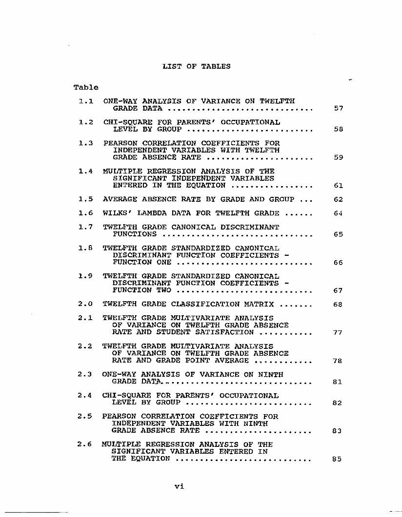
LIST OF TABLES

Table1.1 ONE-WAY ANALYSIS OF VARIANCE ON TWELFTHGRADE D A T A .............................. 571.2 CHI-SQUARE FOR PARENTS' OCCUPATIONALLEVEL BY G R O U P .......................... 581.3 PEARSON CORRELATION COEFFICIENTS FORINDEPENDENT VARIABLES WITH TWELFTHGRADE ABSENCE RATE ...................... 591.4 MULTIPLE REGRESSION ANALYSIS OF THESIGNIFICANT INDEPENDENT VARIABLESENTERED IN THE EQUATION ...... 611.5 AVERAGE ABSENCE RATE BY GRADE AND GROUP ... 621.6 WILKS' LAMBDA DATA FOR TWELFTH GRADE .... 641.7 TWELFTH GRADE CANONICAL DISCRIMINANTFUNCTIONS ............................... 651.8 TWELFTH GRADE STANDARDIZED CANONICALDISCRIMINANT FUNCTION COEFFICIENTS - FUNCTION ONE ............................ 661.9 TWELFTH GRADE STANDARDIZED CANONICALDISCRIMINANT FUNCTION COEFFICIENTS - FUNCTION T W O ............................ 672.0 TWELFTH GRADE CLASSIFICATION MATRIX ...... 682.1 TWELFTH GRADE MULTIVARIATE ANALYSISOF VARIANCE ON TWELFTH GRADE ABSENCERATE AND STUDENT SATISFACTION........... 772.2 TWELFTH GRADE MULTIVARIATE ANALYSISOF VARIANCE ON TWELFTH GRADE ABSENCERATE AND GRADE POINT AVERAGE ..... 782.3 ONE-WAY ANALYSIS OF VARIANCE ON NINTHGRADE DATA................................ 812.4 CHI-SQUARE FOR PARENTS' OCCUPATIONALLEVEL BY G ROUP.......................... 822.5 PEARSON CORRELATION COEFFICIENTS FORINDEPENDENT VARIABLES WITH NINTHGRADE ABSENCE R A T E ...................... 832.6 MULTIPLE REGRESSION ANALYSIS OF THESIGNIFICANT VARIABLES ENTERED INTHE EQUATION ............................ 85

vi

LIST OF TABLES (continued)

2.7 AVERAGE ABSENCE RATE BY GRADE AND GROUP ... 862.8 WILKS' LAMBDA DATA FOR NINTH G R A D E ....... 882.9 NINTH GRADE CANONICAL DISCRIMINANTFUNCTIONS ............................... 893.0 NINTH GRADE STANDARDIZED CANONICALDISCRIMINANT FUNCTION COEFFICIENTS ..... 903.1 NINTH GRADE CLASSIFICATION MATRIX ........ 913.2 NINTH GRADE MULTIVARIATE ANALYSISOF VARIANCE ON NINTH GRADE ABSENCERATE WITH STUDENT SATISFACTION ......... 983.3 NINTH GRADE MULTIVARIATE ANALYSISOF VARIANCE ON NINTH GRADE ABSENCERATE WITH GRADE POINT AVERAGE........... 99

LIST OP FIGURES

FIGURE1. Twelfth Grade Group Assignment ................. 402. Ninth Grade Group Assignment ................... 403. Student Satisfaction Scale ..................... 46

_ * * »v m

CHAPTER I

STATEMENT OF THE PROBLEM

Background of the StudyAbsenteeism has been a major problem within the

secondary schools. There have been increases in both full and partial day absences. The dropout rate has increased while school enrollments have declined. Communities have pressured Board of Education members to increase graduation requirements and to ensure a quality educational program for their children.

This same concern has been shared by legislators across the nation. New York's legislative committee has focused attention on the topic due to its declining economy. The committee perceived this decline to be the direct result of a high dropout rate, especially among the Black youth. California has focused more emphasis on actual attendance reporting due to discrepancies found during a physical audit of randomly selected classrooms.The California State Auditor indicated that actual attendance figures are well below those reported by the various school districts for state aid purposes. Within Michigan, section 49 of the proposed School Aid Act for the 1987-88 school year, states that monetary incentives should be awarded to local school districts who provide positive programs for "high risk" students in order to reduce absenteeism and the dropout rate.

1

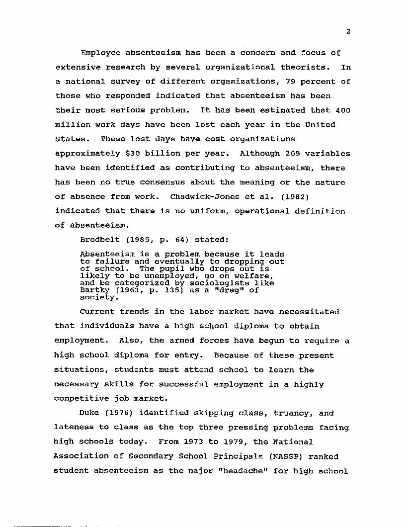
2

Employee absenteeism has been a concern and focus ofextensive research by several organizational theorists. Ina national survey of different organizations, 79 percent ofthose who responded indicated that absenteeism has beentheir most serious problem. It has been estimated that 400million work days have been lost each year in the UnitedStates. These lost days have cost organizationsapproximately $30 billion per year. Although 209 variableshave been identified as contributing to absenteeism, therehas been no true consensus about the meaning or the natureof absence from work. Chadwick-Jones et al. (1982)indicated that there is no uniform, operational definitionof absenteeism.

Brodbelt (1985, p. 64) stated:Absenteeism is a problem because it leads to failure and eventually to dropping out of school. The pupil who drops out is likely to be unemployed, go on welfare, and be categorized by sociologists like Bartky (1963, p. 135) as a "dreg” of society.Current trends in the labor market have necessitated

that individuals have a high school diploma to obtain employment. Also, the armed forces have begun to require a high school diploma for entry. Because of these present situations, students must attend school to learn the necessary skills for successful employment in a highly competitive job market.

Duke (1976) identified skipping class, truancy, and lateness to class as the top three pressing problems facing high schools today. From 1973 to 1979, the National Association of Secondary School Principals (NASSP) ranked student absenteeism as the major "headache" for high school

3

principals. These results were confirmed through a 1977 study by the National Institute of Education where over one-third of the public secondary school principals who responded to the survey rated student absenteeism as either a "serious" or "very serious" problem in the schools (Neill, 1979).

In 1985, De Jung and Duckworth conducted a two-yearstudy on high school absenteeism in an urban schooldistrict located in the western United States. Their results indicated that school absenteeism rates were above expectation. They found that class absences were frequent and quite common throughout the school where the average student missed over 100 classes during the school year.

Student absenteeism has been a pressing problem for one Michigan school district. Vultaggio (1984) stated that200,000 hours of instruction were lost over a period of twenty weeks. His study encompassed seventh throughtwelfth grade students and involved only one semester ofattendance data. On the average, each student missed five full days and fifteen partial days of school during the semester. There was a difference between junior high and senior high absence patterns. The majority of junior high students missed full days; whereas, the majority of senior high students missed partial days of school.

Within the last two decades, considerable research has been conducted on dropouts and potential dropouts. An individual's absenteeism rate has been identified as a variable that predicts dropping out of school. Snepp (1956, p. 52) stated;

4

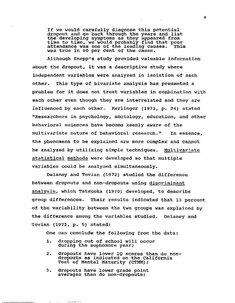
If we would carefully diagnose this potential dropout and go back, through the years and list the developing symptoms as they appeared from time to time, we would probably find that poor attendance was one of the leading causes. This was true in 80 per cent of the cases.Although Snepp's study provided valuable information

about the dropout, it was a descriptive study whereindependent variables were analyzed in isolation of eachother. This type of bivariate analysis has presented aproblem for it does not treat variables in combination witheach other even though they are interrelated and they areinfluenced by each other. Kerlinger (1973, p. 24) stated"Researchers in psychology, sociology, education, and otherbehavioral sciences have become keenly aware of themultivariate nature of behavioral research." In essence,the phenomena to be explained are more complex and cannotbe analyzed by utilizing simple techniques. Multivariatestatistical methods were developed so that multiplevariables could be analyzed simultaneously.

Delaney and Tovian (1972) studied the differencebetween dropouts and non-dropouts using discriminantanalysis, which Tatsuoka (1970) developed, to describegroup differences. Their results indicated that 13 percentof the variability between the two groups was explained bythe difference among the variables studied. Delaney andTovian (1972, p. 5) stated:

One can conclude the following from the data:1. dropping out of school will occur during the sophomore year;2. dropouts have lower IQ scores than do non­dropouts as indicated on the California Test of Mental Maturity (CTMM)?3. dropouts have lower grade point averages than do non-dropouts;

5

4. dropouts tend to be non-white;5. dropouts tend to have more siblings in their families;6. dropouts have skipped more classes than non-dropouts;7. dropouts have received more detentions than non-dropouts.A major shortcoming of the study involved the use of

only one semester of data for the total number of days absent. Although the study included two types of aptitude tests, California Test of Mental Maturity (CTMM) and Differential Aptitude Test (DAT), it excluded any type of achievement test even though past research showed achievement to be significantly related to predicting potential dropouts. By including achievement scores, the researchers might have increased their explained variance between the two groups.

Degrade (1974) conducted an extensive study in Arizona's Mesa School District. The purpose of the study was to develop a profile of the dropout within that school district. Degracie used two separate samples and analyzed over twenty variables. The results indicated a moderately strong relationship (.47) between dropping out of school and the following variables: (a) father in the home,(b) race, (c) Metropolitan Achievement Test score, (d) high school attended, (e) last grade completed, and (f) grade at withdrawal. Although academic aptitude was included in the beginning of the study, it was removed because test uniformity was not evident when data were analyzed from the investigated populations. Though the Metropolitan Achievement Test has a battery of tests that include

6

reading, language, mathematics, science, and social studies, only one score for the total achievement test was used. Therefore, it was impossible to determine the degree of relationship that each content area contributed to dropping out. Although the absence data encompassed a two- year period, only absence rates from secondary school were included.

Curtis (1983) conducted a longitudinal study inAustin, Texas, that encompassed four school years from1977-78 to 1980-81. Discriminant analysis was used todetermine the degree of prediction for dropping out ofschool. There were four groups involved in the analysis.When discussing the results, Curtis (1983) stated:

Students who have low GPA's, who are behind in grade for their age, who have been involved in serious discipline incidents, who are female, and who are non-Black have a higher than average probability of dropping out (p. 7).There were two findings that were contradictory to

previous research in that males dropped out of school moreoften than females and that minority students dropped outof school more often than White students. Curtisrecognized these discrepancies and stated:

Furthermore, the variables included in the formula are very limited in scope. The emergence of sex as a predictor indicates that some variables outside of the scope of the formula affect girls more negatively than boys (p. 7).Achievement scores were omitted from the analysis

because different tests were administered at the junior high and high school level which impeded equating the tests in a systematic manner. Also, special education students were omitted from the analysis due to their grades and GPA values having a different connotation with the same

7

variables for those students not certified special education.

Although extensive research has been done on dropouts and those characteristics that identify them, little research has been done on identifying those variables that account for differences between students who attend school and those who do not attend school on a regular basis. In addition, limited research has been conducted on special education students even though this population has increased during the last decade. Very few studies have encompassed a student's progression through elementary, junior high, and high school although Fogelman (1978) extended the analysis of the National Child Development Study (NCDS) to include sixteen-year-old students. The original study involved all children living in England, Scotland, and Wales who were born during one week in March, 1958. Various follow-up studies focused on seven, eleven, and sixteen-year-old students to determine those variables that relate significantly to school attendance.

With the exception of Fogelman's study of children living in the British Isles, no other longitudinal studies were located that tracked student absenteeism across all three levels of a child's educational career. In addition, one population that Fogelman's study in 1978 did not involve were special education students; whereas, this dissertation included them in the analysis. By developing a profile that assists in predicting student absenteeism, school administrators will be better equipped to detect potential non-attenders and to prevent student absenteeism through the development of positive educational

programs to promote attendance and to reduce absenteeism. These programs should be offered at all levels of a child' educational career.

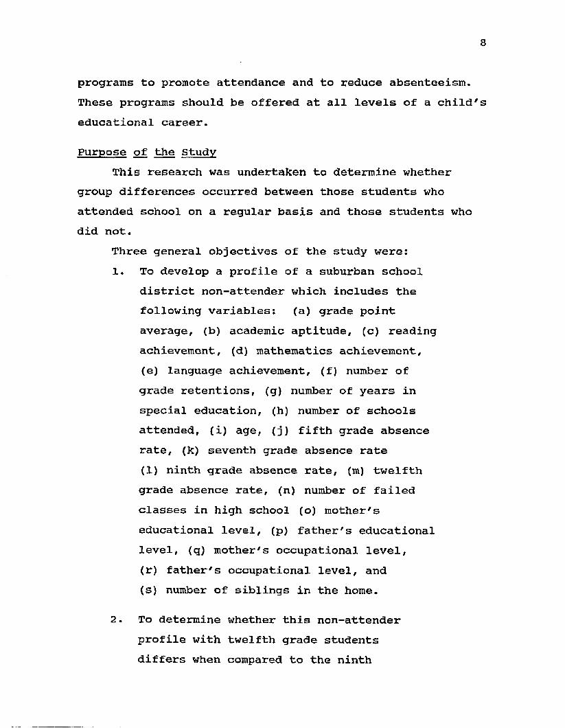
Purpose of the StudyThis research was undertaken to determine whether

group differences occurred between those students who attended school on a regular basis and those students who did not.

Three general objectives of the study were:1. To develop a profile of a suburban school

district non-attender which includes the following variables: (a) grade pointaverage, (b) academic aptitude, fc) reading achievement, (d) mathematics achievement,(e) language achievement, (f) number of grade retentions, (g) number of years in special education, (h) number of schools attended, (i) age, (j) fifth grade absence rate, (k) seventh grade absence rate(1) ninth grade absence rate, (m) twelfthgrade absence rate, (n) number of failedclasses in high school (o) mother's educational level, (p) father's educational level, (q) mother's occupational level,(r) father's occupational level, and (s) number of siblings in the home.

2. To determine whether this non-attender profile with twelfth grade students differs when compared to the ninth

9

grade non-attender from the same school district.

3. To determine by gender whether attenders are more satisfied with school than non-attenders.

Scope of the StudyThis research attempted to analyze by gender group

differences between those students who attend school regularly and those students who attend irregularly. In addition, the study attempted to replicate the profile with ninth grade students to determine whether the model is applicable to junior high students. The purpose of the second sample was to validate the profile developed with twelfth grade student data. The reason for the second sample was due to results of past studies which indicated that students tend to remain in school until sixteen years of age because the law requires them to stay in school until that time (Screiber, 1979). Also, students have a tendency to withdraw from school either in the tenth or eleventh grade as stated by Durkin (1981).

Questions to be answered by the study include:1. Can non-attenders be predicted readily

with data obtained from existing school records?

2. What discriminating variables contribute to group differences between attenders and non-attenders by gender?

3. Do students' absenteeism rates increase

10

as they progress through elementary, junior high, and high school?

4. Do the variables identified in the twelfth grade sample hold constant when student data from the ninth grade are used?

Group assignment was divided into four categories at both the ninth and the twelfth grade levels. These categories were: (a) female attenders, (b) male attenders,(c) female non-attenders, and (d) male non-attenders. In order to answer the previous questions, the following null hypotheses were developed.

Hypothesis One: There is no significantdifference between group assignment for academic aptitude.

Hypothesis Two: There is no significantdifference between group assignment for student achievement.

Hypothesis Three: There is no significantdifference between group assignment for number of grade retentions.

Hypothesis Four: There is no significantdifference between group assignment for the number of years in special education.

Hypothesis Five: There is no significantdifference between group assignment for the number of schools attended.

11

Hypothesis Six: There is no significantdifference between group assignment for age.

Hypothesis Seven: There is no significantdifference between group assignment for student absenteeism rate.

Hypothesis Eight: There is no significantdifference between group assignment for the number of courses failed in high school.

Hypothesis Nine: There is no significantdifference between group assignment for parents' educational level.

Hypothesis Ten: There is no significantdifference between group assignment for parents' occupational level.

Hypothesis Eleven: There is no significantdifference between group assignment for the number of siblings in the home.

Hypothesis Twelve: There is no significantdifference between twelfth grade absence rate and group assignment, twelfth grade absence rate and student satisfaction, and twelfth grade * absence rate and group assignment with student satisfaction.

Hypothesis Thirteen: There is no significantdifference between twelfth grade absence rate and group assignment, twelfth grade absence rate and grade point average category. and twelfth grade absence

12

rate and group assignment with grade point average category.

The associated alternative hypotheses were that there is a significant difference between group assignment and the identified discriminating variables.

Definition of TermsAcademic Aptitude: Refers to an abilitytest developed to assess a student's capability in learning skills taught within the educational program.

Morm-referenced Achievement Test: Refers to atest developed to measure a student's performance in school relative to the performance of other students nationwide. The data derived from this test provide important information when comparing individuals and groups.

Expanded Standard Scores: Refers to scalescores of an interval level that are produced from scores of all levels of the Comprehensive Test of Basic Skills (CTBS). All grade levels are covered by CTBS. These scores are useful when analyzing students' progress throughout their educational careers.

Discriminant Analysis: Refers to a statist­ical technique that analyzes several variables simultaneously. All independent variables are either at the interval or ratio level of

measurement.

Interval data: Refers to data where there areequal distances between the observations. (For example, temperature would be interval data.)

Ratio data: Refers to data where a true zeropoint is evident in addition to equal distances between the observations. (E.g., weight would be ratio data.)

Canonical Discriminant Function: Refers to alinear combination of the discriminating variables and their relative importance in distinguishing group membership.

Student Absenteeism Rate: Refers to thepercentage of time a student is absent from school during one school year. It is calculated by summing the total number of absences from each class and dividing that number by the total number of available hours of instruction for the school year.

Special Education Student: Refers to a studentwho receives special services within the school district due to being certified as visually impaired, physically impaired, emotionally impaired, educable mentally impaired, language impaired, and/or learning disabled through the school district's special education department.

Comprehensive Test of Basic Skills: Refers to a

14

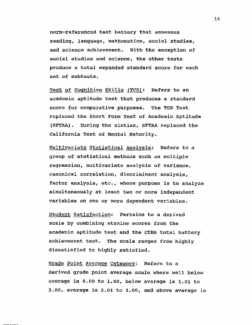
norm-referenced test battery that assesses reading, language, mathematics, social studies, and science achievement. With the exception of social studies and science, the other tests produce a total expanded standard score for each set of subtests.

Test of Cognitive Skills (TCS): Refers to anacademic aptitude test that produces a standard score for comparative purposes. The TCS Test replaced the Short Form Test of Academic Aptitude (SFTAA). During the sixties, SFTAA replaced the California Test of Mental Maturity.

Multivariate Statistical Analysis: Refers to agroup of statistical methods such as multiple regression, multivariate analysis of variance, canonical correlation, discriminant analysis, factor analysis, etc., whose purpose is to analyze simultaneously at least two or more independent variables on one or more dependent variables.

Student Satisfaction: Pertains to a derivedscale by combining stanine scores from the academic aptitude test and the CTBS total battery achievement test. The scale ranges from highly dissatisfied to highly satisfied.

Grade Point Average Category: Refers to a derived grade point average scale where well below average is 0.00 to 1.00, below average is 1.01 to 2.00, average is 2.01 to 3.00, and above average is

15

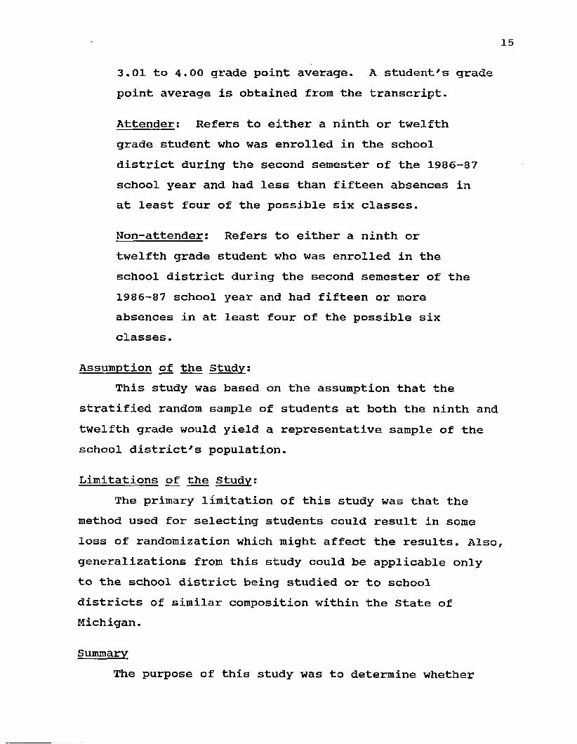
3.01 to 4.00 grade point average. A student's grade point average is obtained from the transcript.

Attender: Refers to either a ninth or twelfth grade student who was enrolled in the school district during the second semester of the 1986-87 school year and had less than fifteen absences in at least four of the possible six classes.

Non-attender: Refers to either a ninth or twelfth grade student who was enrolled in the school district during the second semester of the 1986-87 school year and had fifteen or more absences in at least four of the possible six classes.

Assumption of the Study:This study was based on the assumption that the

stratified random sample of students at both the ninth and twelfth grade would yield a representative sample of the school district's population.

Limitations of the Study:The primary limitation of this study was that the

method used for selecting students could result in some loss of randomization which might affect the results. Also, generalizations from this study could be applicable only to the school district being studied or to school districts of similar composition within the State of Michigan.

SummaryThe purpose of this study was to determine whether

16

group differences occurred between attenders and non- attenders at the twelfth grade level and whether those differences were the same for a second sample of ninth grade students. In addition, this study would indicate the amount of variance between the groups that could be accounted for by the selected discriminating variables.The results from this study could be used to assist school administrators in developing positive educational programs to reduce student absenteeism.

CHAPTER II

REVIEW OF THE LITERATURE

IntroductionIn this chapter, the review has been divided into two

sections. Studies that relate directly to absenteeism are reviewed within the first section. These studies focus on school attendance or excessive absenteeism as the major variables analyzed in the study. Other variables are included in the studies, but they play a secondary role in describing absenteeism. The second section encompasses those studies that refer to absence rates within the context of predicting potential dropouts. Most of these studies include absence rates or school attendance figures as independent variables to determine their relative contribution in predicting school dropouts or identifying potential dropouts.

The Educational Resources Information Center (ERIC) was the source used to locate these studies. Also,INFOTRAC Database was utilized for other articles on absenteeism and dropout rates. Seven books were read to gain a working knowledge of the historical events that have impacted absenteeism during the last century. The most significant event was the inception of the compulsory education law and its revisions throughout the years. This legislation was passed to require that young people attend school to attain the necessary education to increase the

17

18

probability that they will make a successful contribution to society. Following the implementation of this law, attendance officers were hired to enforce the law which then necessitated the establishment of parental schools, more commonly called juvenile homes or detention facilities. Since the turn of the century, educators, parents, and legislators have attempted to devise ways to keep children in school.

Abbott and Breckinridge (1917, p. 92) stated their perceptions on absenteeism.

Children "excused for cause" are, of course regarded by the school authorities not as willful truants, but as non-attending children absent for excusable reasons and therefore not in need of discipline. But the effect of non- attendance is as disastrous to educational progress as is truancy itself, for whether the child's absence is sanctioned by the parents or is in opposition to their wishes, that is, whether the child is a non-attendance or a truant, the effect upon his school work is the same. He misses the school session, falls behind in his school work, and suffers the demoralizing consequences of irregularity.Although this statement was written seventy years ago,

the perceptions of school officials, community members, and parents have remained consistent over the years. They feel that students who do not attend school regularly will have difficulty during their educational careers which will negatively impact the students' contributions to society.

Studies on AbsenteeismZiegler (1928) studied the relationship between school

attendance and school marks and school progress. Data were taken directly from the records of 307 students in seventh grade at a junior high school located in Pennsylvania. The statistics used were: mean, median, sigma, Pearson

19

correlations, critical ratio, and partial correlations.The independent variables studied include: school marks,age-delay (grade retention), distance from school, nationality, socio-economic status (SES), ability, and environment (addresses and their desirability as rated by two local realtors). The dependent variable was school attendance. Ziegler concluded that there was a weak, positive relationship (.23) between school attendance and school marks; whereas, there was not a significant relationship (.13) between ability and school attendance. Also, he found that environment and SES were significantly related to school attendance. Overall, the results indicated that grade point average was a contributing factor to school attendance; however, student ability did not relate significantly.

Snowbarger (1954) for his doctoral dissertation researched those factors associated with truancy among junior high males in Los Angeles, California. The reason for the all male study was due to the reseacher's perception that the male interviewer could establish a greater rapport with male subjects. Five schools were involved in the selection process. Ninety-five students who had four or more unexcused absences during the first semester of the 1953-54 school year, as determined by an attendance officer, were assigned to the truant group. A comparable number of students were assigned to the non­truant group on the basis of sex, school attended, and school grade. The variables studied include: (a) personaladjustment, (b) social adjustment, (c) total life adjustment, (d) school adjustment, (e) family adjustment,

20

(f) community adjustment, and (g) marital adjustment. T- tests were the statistics used in the analysis. There were serious flaws in the methodology of this study. More than one intelligence test was used without any controls put in place to ensure standardization or equating of the tests. This same situation occurred with the achievement tests. Although significant results were found for both intelligence and achievement with school attendance, the results should be interpreted with extreme caution due to these serious flaws within the methodology of this study.

Galloway (1976) studied absenteeism and other pertinent information on children from a large, northern city in England who had a 50 percent absence rate (an arbitrary point set by the researcher) during a seven-week period at the start of the fall semester in 1973. Parochial schools, special schools, and one comprehensive school were omitted from the study due either to the reorganization of the schools or missing student data. Thirty comprehensive schools (similar to secondary schools in America) along with their primary feeder schools (similar to American elementary schools) were involved in the study. The total population involved was 82,779 students (52,908 from primary and 29,871 from comprehensive schools).

Reasons for student absences were identified by the child's education welfare officer; therefore, problems with inter-rater agreement were evident due to a lack of standardization of reasons by the officers. Also, if all absences were due to illness, cases were excluded. Socio­economic hardship was determined by free meals in school. Another variable used in the study was size of the school.

21

Deviant behavior was defined by the number of days a student was suspended from school during May, 1973, to April, 1974. In order to be involved in this analysis, the student had to have been suspended for at least five days. The statistical methods used in the analysis included: percentages, Pearson correlation coefficients, partial correlation coefficients, and the Mann-Whitney U Test.

The results showed that absenteeism rates were less than 1 percent in the primary school years; whereas, there was a 300 percent increase during the first full year of comprehensive school. Free meals related significantly to absence rates in both primary and comprehensive schools. When utilizing the Mann-Whitney U test, the results were consistent with the previous findings. Galloway (p. 46) stated:

The results presented in ... lent no support for the initial hypothesis that persistent absenteeism is a greater problem in large schools than in small ones, nor for the hypothesis that large schools and schools in areas of socio-economic hardship need to exclude more pupils on disciplinary grounds than small schools or schools in socially privileged areas.In conclusion, Galloway's study showed a marked

difference between primary and comprehensive school attendance percentages; whereas, neither school size nor deviant behavior had a significant effect on attendance.

In Galloway's study, the absenteeism data were collected over a relatively short period of time and also at the beginning of the school year. He stated that collecting absenteeism data at the start of the school year could cause an underestimation of a student's absences as Sandon (1961) found absenteeism to be higher during the later months of the school year.

22

Douglas and Ross (1965) conducted a study using test scores and attendance figures from the National Survey of Health and Development, a longitudinal study involving children born in 1946. When these children were eleven- year-olds, they were administered achievement and intelligence tests. The researchers obtained these data for their study. They studied the relationship between composite scores in reading, vocabulary, intelligence, and arithmetic tests and the students' attendance records from the previous four years of schooling. Their results showed a relationship between average scores and attendance with the exception of upper middle class students. Although students in this higher SES group might have missed an excessive amount of school, they performed as well on the tests as those higher SES students who attended school on a regular basis.

These same findings occurred again using data from another national study. Fogelman and Richardson (1974) conducted a study using the National Child Development Survey (NCDS) data for eleven-year-old students. They found that there was a significant relationship between the school attendance level for the current year and reading comprehension, mathematics, and general ability among those test scores of NCDS children whose fathers worked in a manual job. That was the only socio-economic level where the results were significant.

In 1978 Fogelman extended the analysis to include sixteen-year-old students. Not only did Fogelman examine the relationship between school attendance and school attainment (achievement and intelligence) but also

23

adjustment in school and student attendance patterns forboth primary and comprehensive school years. Thestatistical method used was analysis of variance. Thefindings showed a significant relationship between schoolattendance and attainment and behavior. Students who hadhigh attendance rates achieved higher scores on readingcomprehension and mathematics tests. In addition, theirteachers rated them lower on deviant behavior, which wasassessed using the Rutter School Behavior Scale. Althoughthe 1974 results showed social class having a significanteffect on attainment and behavior, these findings did notoccur with the data from the sixteen-year-old students inthe 1978 study.

Fogelman (1978, pp. 157-158) stated:By the time these children were in their final year of compulsory schooling, there was little relationship between their attain­ment and their attendance rate early in the primary school. This is not to suggest that early non-attendance can be ignored (since it does predict later poor attendance, and such continued absence is related to low attainment). It is in fact a rather optimistic finding, suggesting as it does that a child who misses even a considerable amount of school at an early age will be able to overcome any resulting disadvantage through subsequent regular attendance.Fogelman stated that there was difficulty with

comparing overall attendance rates at the ages of seven, eleven, and sixteen due to the changes in the law. In 1978 the legal age to withdraw from school in England was increased from fifteen to sixteen years of age.

Eaton (1979) conducted a study to determine which factors contributed to persistent absenteeism in the upper junior and lower secondary age groups. There were 90 students in the nine-to-eleven-year-old age group and 100

24

in the twelve-to-fourteen-year-old age group. These randomly selected students were from Birmingham, England. Questionnaires were distributed to determine how these students perceived their relationship with their parents, their teachers, and their peers. Also, the students' anxiety level was measured. Other information was collected from student records. Multiple regression analysis was used to determine whether these relationships and student anxiety level were significant factors that contributed to student absences in the junior high and lower secondary high schools.

The results showed that the variables being studied accounted for 23 percent of the total variance for the nine-to-eleven-year-old group; whereas, 34 percent of the variance was accounted for with the twelve-to-fourteen- year-old group. "Relationship with peers" was the variable that explained the most variance (14%) in student absenteeism at the junior high level. "Relationship with teachers" was the variable that accounted for the most variance (21%) of absenteeism at the lower secondary school level. Ability (as determined by intelligence quotients, reading ages, and teacher assessments) accounted for approximately 6 percent of the explained variance in absenteeism for both groups. In addition, ability was the second variable entered into the regression equation for both groups. The predicted value between the students' relationship with parents and school attendance was minute for both age groups. This finding contradicted previous research regarding home-related factors and relationship with parents. Eaton (p. 240) stated:

25

The selection of "relationship with teachers" and "relationship wxth peers" as the dominant variable at the secondary and junior high level respectively adds support to the work of Eaton & Houghton (1974) who concluded that persistent absence is likely to be caused or pre­cipitated by features of a school's society.Although Eaton's major finding was in direct contrast

to previous research dealing with home-related factors and parental relationship, he did learn that ability also was a contributing factor to student absenteeism. He recommended that further research on absenteeism should be conducted at the early-age level. However, caution should be exercised when interpreting the results on ability level due to teacher assessments being included. This situation could cause problems with internal validity due to the selection procedures used.

Studies on DropoutsPenty (1956) studied reading ability and high school

dropouts with 1,186 students (593 poor readers and 593 goodreaders as determined by an arbitrary point on the IowaSilent Reading Test) involved in the study. These studentsattended high school in Battle Creek, Michigan. When thegroups were compared, the results indicated that poorreaders dropped out of school more often than good readers.Penty found that tenth grade was the most frequent gradefor withdrawal. When academic performance was analyzed,Penty (p. 53) stated:

The difference between the mean intelli­gence quotients of the poor readers who graduated, based on the Otis Test of Mental Ability, was not large enough to account for the difference in academic progress. The I.Q of the

26

graduates was 88.2 and of the dropouts 83.6. At the lowest quartile, theI.Q. of the dropouts was 5.0 points lower than the I.Q. of the graduates dropouts 76.0; graduates 81.0).Statistically,however, the difference between the mean intelligence quotients of the poor and good readers was significant at the .01 level.Penty's study showed significant results when

analyzing group differences other than intelligence. Pentystated that a different ability test might have made adifference because the Otis Test of Mental Ability reliesheavily on the student's ability to read. The independentvariables were not analyzed simultaneously as t-tests werethe statistical methods used in her study.

Green (1958) conducted a dropout study of ninththrough twelfth grade students for his doctoraldissertation. The chi-square statistic and multipleregression analysis were the methods used in the analysisto determine the relationship between school dropouts andgrades, ability, and achievement. The findings indicatedsignificant relationships between school dropouts andschool persisters on average intelligence scores, gradepoint averages, and the mean scores on the subtests of theIowa Tests of Educational Development.

Green concluded that the dropouts performed lower onachievement tests, exhibited poorer academic capabilities,and received lower grade point averages than those studentswho remained in school.

Nachman, Getson, and Odgers (1964) conducted a studyof high school dropouts in Ohio. It was a descriptivestudy where the findings indicated that very fewcharacteristics can describe or identify potential

27

dropouts due to the complexity of the "dropout" concept.The researchers found that several variables significantlyimpacted a student's decision to drop from school. Thestudy included only dropouts; therefore, generalizations toother populations are limited. Comparisions between thosestudents who remained in school and those students whodropped out cannot be made because data were not collectedon the remainder of the school population. Nachman,Getson, and Odgers (1964) stated that:

Another phenomenon which appeared related to dropping out of school was the existence of a pattern of deterioration with respect to marks received and attendance and dis­cipline problems exhibited as the future dropout progressed through school (p. 52).The study covered grades nine through twelve. The

findings from the study showed that ninth grade students had higher absence rates and more disciplinary contacts than either the eleventh or twelfth grade students.This situation lead the researchers to conclude that dropouts tended to leave school as soon as legally possible; otherwise, eleventh and twelfth grade students would have the same type of patterns. The researchers questioned whether the eleventh and twelfth grade students may have different motives for dropping out of school. The researchers recommended that a comparative study be conducted on the differences between dropouts and non­drop outs .

The Orange County Dropout Prediction study (1965) was conducted to determine those factors which could predict a potential dropout at the sixth-grade level. The selection involved 200 elementary schools where 2,400 students who represented sixteen school districts were included in the

28

analysis- The sample mortality rate was 61 percent for the "random" group, 66 percent for the "least likely to drop from school" group, and 45 percent for the "most likely to drop from school" group. These students were selected into these groups by their elementary school principal, their teacher, and the school nurse. These school officials were to collectively select four students for each group, and there had to be an equal representation of gender within each group.

The purpose of the study was to identify those factors that could potentially predict dropouts in the sixth grade and to determine whether or not elementary officials could accurately predict potential dropouts.

The multiple regression analysis showed a moderately strong association (.39) between a combination of the best predictors of academic variables and trait variables with school officials* selection of students as either dropouts or graduates from the random group. Discriminant analysis was used to determine how well these children were assigned to either the dropout or the graduate category from the random group. The discriminating variables were: attendance record, CTMM total IQ score, math GPA, citizenship average, academic GPA, and four teacher estimate traits (authority, responsibility, behavior, and abstract concepts). One hundred and twenty-two out of 168 graduates in the random group (73%) were classified correctly. Thirty-nine of the forty-eight dropouts (81%) were classified accurately. These results should be viewed with caution due to the selection procedures used in the study as this could impact control of internal validity.

29

The results from the Orange County Prediction study indicate that intelligence, grade point average, and certain teacher estimate traits contribute to the identification of potential dropouts in the sixth grade.

In 1966 the Prince George County Schools established Project DIRE (Dropout Identification, Rehabilitation, and Education) through the assistance of the Educational Service Bureau. The staff conducted a descriptive study to identify potential dropouts through the use of readily available data from school records and from student interviews. The sample consisted of 1,621 dropouts from the secondary schools' total population of 44,660 during the 1965-66 school year. The results indicated that:(a) dropouts were enrolled in the tenth or eleventh grade when they withdrew, (b) dropouts were either sixteen or seventeen years old, (c) dropouts missed twenty or more days during the school year, (d) the majority of dropouts were receiving passing grades, (e) the dropouts had average to better than average ability, (f) the dropouts' reading and math achievement were below average, and (g) a majority of the dropouts had been in the school system at least six years.

These findings appear to confirm other studies with the exception of intellectual ability. The lack of mobility of the dropouts is another conflicting finding of this study when compared to other studies that showed mobility to be higher for dropouts than for graduates.

Dudley (1971) conducted a dropout-prediction study in the Indiana Public Schools. The purpose of the study was to determine whether dropouts differed from graduates on

30

several characteristics. School officials were to randomly select fifty dropouts and fifty graduates from their records and complete a twenty item biographical questionnaire on each student. They identified 1,090 students. Achievement and ability scores were standardized for purposes of test validity. The first analysis consisted of a stepwise discriminant analysis. The researcher recognized that there would be difficulties using discriminant analysis with categorical measures as the method requires at least interval data. Dudley used a procedure to alleviate that problem and stated that this procedure had been documented by Gross et al. (1958) and Mayer (1963). Dudley (p.23) stated "An analysis procedure was therefore introduced that produced weights corresponding to the relevant relationship between and among the dependent variables." The chi-square statistic was the procedure used in the analysis. The results showed that the two groups differed on several variables such as grade point averages, peer acceptance, intelligence quotients, and parents7 educational level. He stated that the predictive variables were readily obtained from school records. Also, several variables analyzed simultaneously could predict potential dropouts more efficiently than variables analyzed individually.

Dudley stated that caution should be exercised when interpreting the results as only two-thirds of the selected random sample completed the data-gathering forms.

Spencer (1975) attempted to describe the potential dropout by using the most complete data from the student's academic file. A random sample of 25 percent (4 03) of the

31

1,612 potential dropouts from fifteen secondary schools located in Norfolk, Virginia, were included in the analysis. He concluded that the average dropout was at least two years behind academically when compared to peers. The average dropout had a high absentee rate (41%) which significantly impacted academic achievement. There was a higher percentage of mothers in the home when compared to fathers in the home. Also, there was a higher referral rate for dropouts to special educational agencies (e.g., vocational education, adult education, and special education). Factors that contributed to withdrawal from school were low GPA, low academic achievement, and low academic aptitude. Again, this study was descriptive in nature.

Schrom (1980) studied factors that influence ninth grade students' intentions to leave secondary school in Victoria, Australia. Discriminant analysis was used to determine group differences on family background variables, school characteristics, significant others, personal assessments, and attitudes on school-leaving intentions.The sample involved 2,300 students. The results showed that school characteristics and family background variables had little effect on the school-leaving intentions of ninth grade students. The major influence on these students and their intention to leave school centered on their parents' wishes for them to remain in school. Strom stated that these findings are supported by previous research conducted by Poole (1978a). Schrom (p. 13) further stated that "The finding that family background and school characteristics have little effect on intentions to leave school is

32

unexpected and contrary to the findings of other research." Although little difference occurred between male and female students' perceptions on parental attitude towards their children leaving school, other discriminant analysis functions showed a difference with gender.

When Schrom discussed these results, she stated that the reasons for the difference with other studies could be that previous studies did not include all of the background or attitudinal variables that her study used or that other studies analyzed variables in isolation of each other.

Another study on student absenteeism and schooldropouts was conducted in Canada during the mid-seventies.The researchers, Crespo and Michelena (1981, p. 40) stated:

Absenteeism and dropping out are at the forefront of the educational scene in Quebec. These problems are not new; what is new is the strong emphasis that govern­ment officials and educators are now placing upon the early detection of potential drop­outs and follow-up of chronic absentees.Their study was based upon a census of registered

students who attended secondary schools located within theFrancophone area, which is classified an urban area, duringthe 1974-75 school year. Student records were used todetermine a set of variables for the study. The variableswere: (a) absenteeism, (b) academic performance, (c) age,(d) dropping out, (e) intellectual ability, (f) type ofschool, and (g) streaming. The researchers definedstreaming as tracking students into slow, average, andenriched educational programs. Family and SES variableswere excluded from the analysis due to the questionablevalidity of the information from student records. They

33

recognized the important contribution of those variables to absenteeism but did not want to jeopardize findings from their study because of invalid data. These data were analyzed by using measures of association. Zero-order gamma was used with the streaming variable; whereas, partial gammas were used with streaming when the other variables were controlled. Also, multiple regression analysis and path analysis were used.

The results indicated that little difference occurred with streaming, absenteeism, and dropping out when age, intellectual ability, academic performance, and type of school were controlled in the analysis. In addition, the explained variance for streaming and academic performance with absenteeism were 37 percent and 30 percent, respectively. Intellectual ability was the most important factor for academic performance; whereas, age was a minor factor. They found that the type of school had little influence. The path analytic model of absenteeism and dropping out explained only 3 percent of the variance in absenteeism. The researchers perceived that the results could have occurred due to the fact that the absenteeism data were collected during the same year as withdrawal data. Also, they thought that excluding family variables could have had an impact on the results. They felt that streaming should not be discounted as a viable educational program because of the findings from this study.

De Jung and Duckworth (1985) conducted a study on absenteeism in six high schools. They were four-year, comprehensive high schools with enrollments of 1,000 to 1,600 students and sixty to seventy full-time teachers.

34

Data were collected from student records and throughinterviews and questionnaires. The sample size for thefirst year of the study was 8,000 students and 350teachers. These findings are from the first year as theresults from the second year have not been published asyet. The researchers had difficulty measuring absencesbecause records were not as accurate as they should havebeen due to: (a) no consistent procedure for recordingabsences in the classroom, (b) errors that were made whentransferring absences from teacher record books to officerecords, (c) varying perceptions by school officials as tothe definition of full and partial day absences, and (d) noofficial records of class absences. They (p. 15) stated:

The most distressing fact about studentabsences is the volume: nearly every dayin each of our six schools 25 to 30 percent of the students were reported absent from one or more classes. A typical student averaged two to four class absences per week which adds up to over 100 classes missed in a 36-week school year— the equivalent of 18 full days.Students were divided into three groups (top, middle,

and lower) depending upon their average absences. The questionnaire responses showed that nearly all students expected to graduate. In addition, a high number ofstudents stated that they would not drop out of school ifthey had the option. De Jung and Duckworth found that penalties for frequent absences were of little concern to students as they perceived that the rules were not enforced consistently. The researchers stated that GPA was a discriminating factor between the top and lower absence groups. Also, they found that failed courses related to school grades and to school attendance.

35

SummaryThe studies on absenteeism indicated that grade point

average, and achievement (reading and mathematics) have a significant impact on student attendance; whereas, school size does not significantly relate to student absenteeism. As stated in the literature section, there have been conflicting conclusions on the significant impact of student ability with school attendance.

The dropout studies showed that students tended to withdraw from school during the tenth grade and are sixteen years of age. Furthermore, intelligence, achievement in both reading and mathematics, grade point average, and absence rate have a significant relationship with a student's decision to drop from school. Disciplinary contacts and higher absence rates were more prevalent in ninth grade students than with eleventh and twelfth grade students in one study. Mobility did not surface as a significant variable with school attendance or dropping out of school. Although these studies covered a thirty-year period, most of them were descriptive in nature.

This study included descriptive and inferential statistics to describe group differences and to make inferences regarding the population from which the samples were drawn.

CHAPTER III

METHODOLOGY

IntroductionThe purpose of this study was to determine by gender

whether group differences were evident between students who attend school regularly and students who attend irregularly. The general objective was to develop a profile of a suburban school district non-attender by utilizing student data from school records.

Ninth and twelfth grade students were classified as either attenders or non-attenders by the number of class absences they had during the second semester of the 1986-87 school year. Once the students were assigned to either the attender or the non-attender group, they were then divided by gender. Nineteen independent variables were selected based upon the analysis of previous studies discussed in the literature review. The first phase of this study consisted of developing a profile of the non-attender using twelfth grade students and obtaining data readily available from the students' school records. The second phase of this study attempted to replicate the twelfth grade profile with ninth grade student data to determine the applicability of the model with junior high students. One variable, twelfth grade absence rate was not used in the ninth grade analysis because these students had not yet entered high school.

36

37

Questions that were answered by the study include:

1. Can non-attenders be predicted readily with data obtained from existing school records?

2. What discriminating variables contribute to group differences between attenders and non- attenders?

3. Do students' absenteeism rates increase as they progress through elementary, junior high, and high school?

4. Do the variables identified in the twelfth grade sample hold constant when student data from the ninth grade are used?

This chapter describes the site for the study, the selection of the sample, the procedures for data collection, refined definitions of both the dependent and independent variables, a review of the statistical methods used, and a discussion of the appropriate computer package and programs for analyzing the data.

Site of the StudyA large (12,000 students) suburban school district was

selected for the study. The school district is located in Oakland County and is part of the southeast Michigan metropolitan area. The district could be considered typical in the State of Michigan due to the following reasons. The student achievement test scores on the Michigan Educational Assessment Program (MEAP) have been comparable to the State's averages over the years.Students, on the average, tend to score slightly above the

38

national averages on norm-referenced measures of achievement and these results have been consistent annually.

The district experienced a yearly decline in enrollment of approximately 500 students per year over the past few years. Also, the district has seen a reduction in funding at the State level. A wide variety of socio­economic groups reside within the boundaries of the school district; however, the district is composed primarily of White, middle-class, "blue-collar'1 families. These demographic characteristics tend to compare with many other Michigan school districts; therefore, the findings may be applicable to groups outside this school district.

Selection of the SampleDuring the second semester of the 1986-87 school year,

there were 877 twelfth grade students enrolled at the two high schools (grades ten through twelve) and 829 ninth grade students enrolled at three of the junior high schools (grades seven through nine). The sample was divided into two groups classified as attenders and non- attenders. For the purpose of this study, a student who had less than fifteen absences in at least four of the possible six classes during the second semester of the 1986-87 school year was assigned to the attender group. A student who missed fifteen or more days in at least four of the possible six classes during the same second semester was assigned to the non-attender group. Once this assignment occurred, the groups were then divided into males and females.

39

Within the twelfth grade sample, there were 795 attenders (91 percent) and 82 non-attenders, who constituted 9 percent of the total twelfth grade population within this school district. The non-attender sample consisted of forty-seven males (57%) and thirty-five females (43%). To ensure a large enough sample for the analysis, all non-attenders were included in the study even though this situation could impact internal validity due to selection procedures. Comparable proportions of both males and females were randomly selected from the attender group by using the systematic sampling technique. The fifth person on both the male and female listings was selected as the starting point and every tenth person was selected until the necessary sample sizes for each gender were obtained.

Within the ninth grade sample, there were 746 students assigned to the attender group (90 percent) and 83 students assigned to the non-attender group, who encompassed 10 percent of the total ninth grade population. In the non- attender group, there were 45 males (54%) and 38 females (46%). Again, the lists were subdivided by gender and comparable proportions were obtained for the attender group. The systematic sampling technique was used to obtain the necessary sample sizes where the tenth person on each list was selected for the starting point and every fifteenth person was selected after that to obtain the correct sample size.

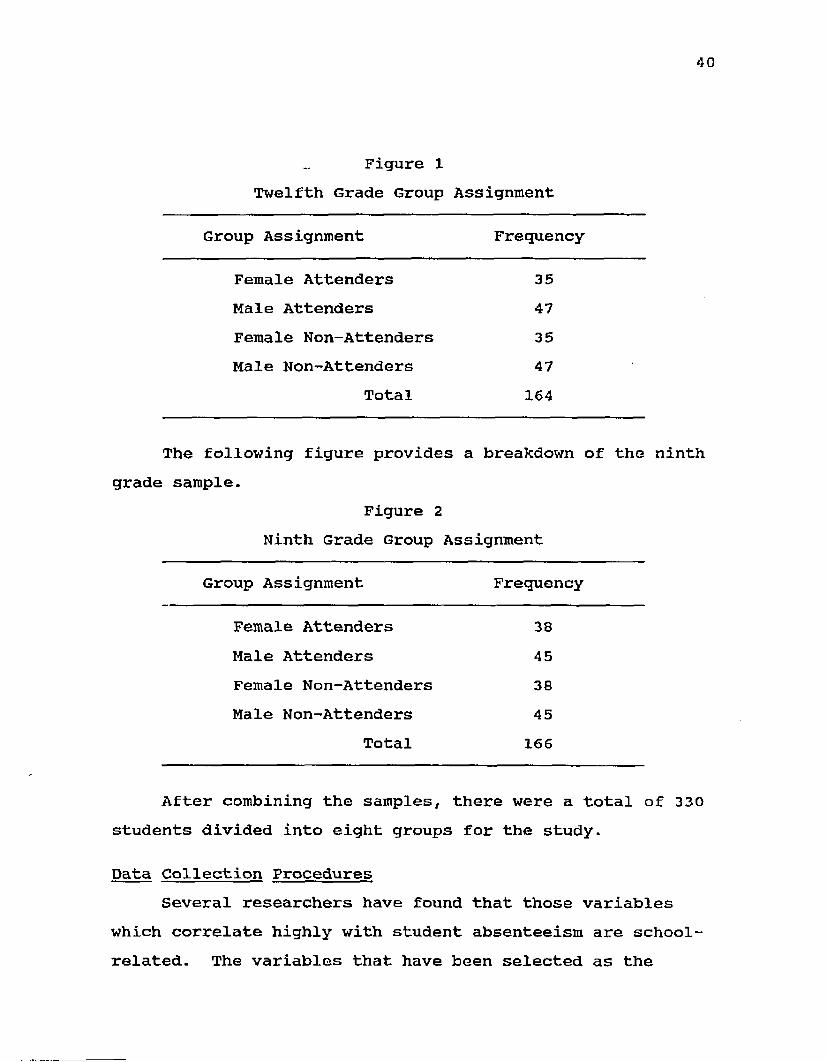
At the end of the selection procedure for both grade levels, there were four groups identified at each grade.

40

Figure 1 Twelfth Grade Group Assignment

Group Assignment Frequency

Female Attenders 35Hale Attenders 47Female Non-Attenders 35Male Non-Attenders 47

Total 164

The following figure provides a breakdown of the! sample.

Figure 2Ninth Grade Group Assignment

Group Assignment Frequency

Female Attenders 38Male Attenders 45Female Non-Attenders 38Male Non-Attenders 45

Total 166

After combining the samples, there were a total of 330 students divided into eight groups for the study.

Data Collection ProceduresSeveral researchers have found that those variables

which correlate highly with student absenteeism are school- related. The variables that have been selected as the

41

independent variables in this study are quite similar to those variables used in previous studies discussed in the literature section. The dependent variables include gender and group assignment based upon class absences.Researchers have studied gender in both absenteeism and dropout studies. Their findings indicate that males tend to drop out of school more often than females.

Although absence rates and school attendance figures have been studied previously, there has not been a consistent standard set for determining regular and irregular school attendance. For the purposes of this study, an arbitrary point of 15 absences per class in at least four classes out of a possible six was used. The reasons for this arbitrary point were that the school district has approved an attendance policy that sets fifteen absences within a class as the cut-off point for receiving credit in class and that this arbitrary point was used by Vultaggio in 1984 when he conducted the descriptive study on student attendance within the school district.

Data were obtained through the Office of Management Information Systems after the Director approved the study. Since most of the information was obtained directly from files maintained by the Management Information Systems Office, the data were coded to preserve students*

anonymity. Data were collected only by the researcher to maintain consistent data collection procedures. The information collected on all variables for each student were compared on three different occasions to ensure accurate data. If any questionable data surfaced, then the

42

student's school record was reviewed for accuracy.

Dependent VariablesGender. This variable has been used as an independent

variable in several of the studies on dropouts and student absenteeism. Researchers have concluded that there is a difference between males and females on dropping out of school and on attending school regularly. Because of these findings, gender was used as one of the dependent variables for determining group assignment. This dependent variable was used to determine whether or not there were independent variables which discriminated between attenders and non- attenders that were unique to gender.

Attendance group. The researcher set the arbitrary point for attender and non-attender based upon the attendance policy approved by the school district's board of education members. This attendance policy had been in existence for at least four years. The determination of four classes out of six classes was established by the program evaluator who conducted an absenteeism study during the first semester of the 1984-85 school year.

Data for both of the dependent variables are at the nominal level of measurement which is the appropriate level for the statistical procedure to be used on the data.

Independent VariablesAs stated previously, these independent variables are

consistent with variables used by other researchers in studying dropouts and student absenteeism. The data used were collected routinely by officials within the school

43

district.

Grade point average (GPA). This variable was obtained from the student's official transcript located in the Management Information Systems Office. It was computed by summing the number of attempted credits and multiplying that total number by the weighted grade point for each class to obtain the grade point average. Attempted credits are defined as those classes that a student was enrolled in during the semester. If the student dropped or failed the class, those classes would still be reflected in the student's GPA.

Academic aptitude. This variable referred to the total standard scale score from a norm-referenced test.The Test of Cognitive Skills (TCS) score was used for the ninth grade students; whereas, the Short Form Test of Academic Aptitude (SFTAA) score was used for twelfth grade students. The reason for the difference is that the TCS replaced the SFTAA in the school district's testing program during the spring of 1983. The test publisher equated the two tests for the purpose of enabling school district personnel to continue to use the annual data in comparing student progress throughout the years. Students were tested at the third, fifth, and eighth grade levels on both the academic aptitude test and the CTBS achievement test. The TCS test and the SFTAA test were designed to assess the intellectual capabilities of students and to predict students' potential rate of progress as well as their level of success. These tests measure academic aptitude through several items on a multiple-choice test that covers

44

sequencing, analogies, and memory. Data for both the academic aptitude variable and the achievement variables were obtained from testing files located in the Management Information Systems Office.

Reading achievement. This variable encompassed the total reading score on the Comprehensive Test of Basic Skills (CTBS) test. Form U of the CTBS test battery replaced form S in the school district's testing program in the spring of 1983. The results for the twelfth grade students were from form S; whereas, the results for the ninth grade students were from form U. Again, the test publisher equated the two tests to ensure that school districts could compare student results throughout the students' educational careers. CTBS is a norm-referenced, multiple-choice test designed to measure student achievement on those skills that are generally taught within a school district's curricula. CTBS is given at the same grade levels as the TCS and the SFTAA and is given at the same time of the year. The reading section of the CTBS battery includes reading vocabulary and reading comprehension. The expanded standard score was the measurement used for this variable as well as the next two variables which are mathematics and language achievement.

Mathematics achievement. This variable included the total expanded standard score for the mathematics section on the CTBS test battery. The mathematics section covers math computation, math concepts, and math applications. Again, form S was used for twelfth grade and form U for ninth grade.

45

Language achievement. This variable consisted of the expanded standard score from the CTBS test battery for the total language section of the test. The language section of the test includes spelling, language mechanics, and language expression.

CTBS total battery achievement. This variable encompassed the combined results of the reading, language, and mathematics achievement. This score would be used in the analysis regarding student satisfaction. It is reported in expanded standard score and in stanine.

Student satisfaction. This variable encompassed a rating satisfaction scale by matching stanine scores on the academic aptitude test with the CTBS total battery achievement test. The stanines from both tests were ranked from low to high with the low scale encompassing stanines one to three (1-3) on either test. The average scale consisted of stanines four through six (4-6) on either test. The high scale contained stanines of seven, eight, and nine (7-9). Once the new aptitude/achievement score was developed, the five ratings on the satisfaction scale were derived by combining the low to high rankings. In the testing manual for the CTBS test battery and for the academic aptitude test, stanines have been categorized into ordinal levels of measurement. In addition, a derived score for anticipated achievement has also been developed by the testing director of Oakland Schools. His approach was to use the analysis of variance procedure to determine whether or not students were achieving according to their abilities as tested on these two different tests. This

46

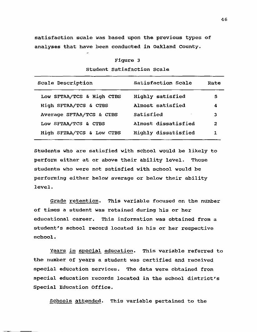
satisfaction scale was based upon the previous types of analyses that have been conducted in Oakland County.

Figure 3 Student Satisfaction Scale

Scale Description Satisfaction Scale Rate

LOW SFTAA/TCS & High CTBS Highly satisfied 5High SFTAA/TCS & CTBS Almost satisfied 4Average SFTAA/TCS & CTBS Satisfied 3Low SFTAA/TCS & CTBS Almost dissatisfied 2High SFTAA/TCS & Low CTBS Highly dissatisfied 1

Students who are satisfied with school would be likely to perform either at or above their ability level. Those students who were not satisfied with school would be performing either below average or below their ability level.

Grade retention. This variable focused on the number of times a student was retained during his or her educational career. This information was obtained from a student's school record located in his or her respective school.

Years in special education. This variable referred to the number of years a student was certified and received special education services. The data were obtained from special education records located in the school district's Special Education Office.

Schools attended. This variable pertained to the

47

number of schools a student attended throughout the years. The information was located in the student's school record on file in the appropriate school building.

Age. This variable referred to the age of the student during the 1986-87 school year and was calculated by subtracting the student's year of birth from that current school year.

Fifth grade absence rate. This variable was calculated by summing the number of days a student was absent while attending the fifth grade and multiplying that number by the hours of instruction lost for each day. Once that figure was obtained, the absence hours for the student were then divided by the total number of available hours of instruction for the year as reported on an annual form submitted to the State of Michigan entitled "Report of Days of Instruction" (form RI-4701). This proportion was then multiplied by 100 to obtain a percentage that was the student's absence rate for that school year.

Seventh grade absence rate. This variable was calculated by summing the number of absences within classes for the school year and then dividing the number by the total available hours for instruction as stated on the State form (RI-4701). The proportion was then multiplied by 100 to obtain a percentage, which was the student's absence rate for that year. Data were obtained from the official school transcript extracted from files in the Management Information Systems Office.

Ninth grade absence rate. This variable was calculated

48

in the same manner as the seventh grade absence rate except that it used the student's absences from classes attended during the ninth grade.

Twelfth grade absence rate. This variable referred to the student's absence rate in the twelfth grade. It was calculated in the same manner as was the ninth and the seventh grade absence rates. This variable was omitted from the ninth grade profile as those students had not yet attended high school.

Failed classes in high school. This variable referred to the number of classes a student failed during his or her high school career. The students' transcripts were used.

Mother's educational level. This variable was obtained from the student's cumulative record and is reported in the number of years of education.

Father's educational level. This variable referred to the number of years of education for the student's father and was extracted from the student's cumulative record.

Mother's occupational level. This variable was obtained from the student's cumulative record. It indicated the level of employment for the mother.Occupation ratings were assigned according to the categories defined in the Directory of Occupational Titles.

Father's occupational level. This variable referred to the father's occupational level. It was obtained in the same fashion as the mother's occupational level.

49

Number of siblings. This variable was collected from the student's cumulative record. It indicates the number of brothers and/or sisters that reside with the student.

With the exception of parents' occupational level, data were at the interval level of measurement, a requirement for the statistical method to be used in the analysis.

Statistical MethodsIt was important to understand the basic structure of

the data set prior to analyzing the data using a multivariate statistical procedure. There are several statistical procedures that have been applied to determine the data structure at both grade levels. Frequency counts and percentages were included for each variable along with graphic displays that present a visual interpretation of the data set. Mean values, standard deviations, and intercorrelations have provided the necessary statistical descriptions. These types of descriptive information were generated by using SPSS PC+ (Statistical Package for the Social Sciences), the computer package used on a personal computer.

Multiple regression analysis was the multivariate statistical technique for analyzing student absenteeism over the years in elementary, junior high, and high school. Again, SPSS for the personal computer was used for the analysis.

Discriminant analysis was the statistical procedure used in analyzing the data at both grade levels so that

50

the ten hypotheses could be tested. This statisticaltechnique not only attempts to maximize the discriminationbetween the members of each group, but also attempts tocorrectly assign each group member through classification.Kerlinger (1973, p, 650) stated:

Although discriminant analysis has not been used much in behavioral research, it has interesting potentialities. It can be used in two main ways:(1) as a classification and diagnosis method, and(2) to study the relations among variables in different populations and samples.Discriminant analysis is the most appropriate

technique for determining whether or not group differencesexist between attenders and non-attenders and whether ornot those differences are unique to gender. Parents'occupational level was not tested with discriminantanalysis due to the data being at the nominal level ofmeasurement which would be a violation of the statisticalprocedure. In addition, another concern centered on theinaccuracy of these data due to the inconsistency of therecords being updated by school officials on a regularbasis. The chi-square procedure was used to analyzeparents' occupational level so that the hypothesis could betested. SPSS for the personal computer was used for thisanalysis. The level for determining statisticalsignificance was set at the .05 alpha level.

Computer PackageThe Statistical Package for the Social Sciences was

the computer package used to analyze the data. SPSS is awidely used computer program package that has thecapability of analyzing data at both the univariate andmultivariate levels. SPSS was developed at Stanford

51

University in 1965 and since that time has been revised so that the most current methods, design, and programs are available in the computer program package. Not only is there a package for the mainframe computer but also for the personal computer, which was used for these analyses.

SummaryThe purpose of the study was to determine group

differences between attenders and non-attenders and whether or not those identified discriminating variables were unique to gender. A large suburban school district was the site for this study. There were 82 non-attenders identified at the twelfth grade level; therefore, a comparable group of 47 males and 35 females were randomly selected from the attender group. The total sample for thetwelfth grade was 164 students. There were 83 non-attenders identified at the ninth grade level; therefore, a comparable group of 45 males and 38 females were randomly selected from the attender group. The total sample for the ninth grade was 166 students. When combining the total for both grade levels, there were 3 30 students involved in the study.

In order to have a large enough sample for theanalysis, the researcher decided to include all of the non-attenders. Because of the decision to include all of the non-attenders rather than randomly selecting from each grade level, internal validity could be impacted due to the selection procedures.

Seventeen independent variables at the interval level of measurement were identified through a review of the literature. These variables were similar to variables that

52

were identified with either student absenteeism or school dropout characteristics in previous studies. With the exception of one variable (twelfth grade absence rate), all variables were used at both grade levels.

Descriptive statistics were applied on the data prior to any multivariate statistical procedures. The purpose for using descriptive statistics first was to obtain a better understanding of the data set before applying inferential statistics on the data. Multiple regression analysis was the statistical procedure used to determine whether or not there was a relationship between student absence rates and student progression through elementary, junior high, and high school. In order to test ten hypotheses stated in Chapter I, discriminant analysis was the multivariate statistical procedure used in the analysis. The other three hypotheses were tested by using either the chi-square statistic or multivariate analysis of variance. SPSS for the personal computer was the program package used to analyze the data.

CHAPTER IV

RESULTS AND DISCUSSION

IntroductionThe results from the data collection and analyses

discussed in Chapter III are presented in this chapter. Printouts for each statistical procedure are included in the Appendices. Appendix A through Appendix G include twelfth grade data; whereas, Appendix H through N include the ninth grade data. This chapter is divided into two sections where results from each grade level are discussed separately. Within each section, explanatory statements are given for the data. The Statistical Package for the Social Sciences (SPSS) for the personal computer was used to test the hypotheses and to generate both descriptive and inferential data.

Testing of the HypothesesTen hypotheses focused on determining group

differences between attenders and non-attenders by gender through the collective contributions of several independent variables. Discriminant analysis was the statistical procedure used to test the following ten hypotheses.

Hypothesis One: There is no significantdifference between group assignment for academic aptitude.

Hypothesis Two: There is no significant

53

difference between group assignment for student achievement.

Hypothesis Three: There is no significantdifference between group assignment for the number of grade retentions.

Hypothesis Four: There is no significantdifference between group assignment for the number of years in special education.

Hypothesis Five: There is no significantdifference between group assignment for the number of schools attended.

Hypothesis Six: There is no significantdifference between group assignment for age.

Hypothesis Seven: There is no significantdifference between group assignment for student absenteeism rate.

Hypothesis Eight: There is no significantdifference between group assignment for the number of courses failed in high school.

Hypothesis Nine: There is no significantdifference between group assignment for parents1 educational level.

Hypothesis Eleven: There is no significantdifference between group assignment for the number of siblings in the home.

55

The other three hypotheses were tested by different statistical procedures and are so noted in the body of the text. Parents' occupational level was tested using the chi-square procedure; whereas, student satisfaction and grade point average were tested by multivariate analysis of variance.

Preliminary steps to testing those hypotheses are provided in each section prior to the explanatory statements on the discriminant analysis procedure. Within all these analyses, students who had missing data were excluded as reflected by the size of the groups (N). The level of significance was set at the .05 alpha level.

Twelfth Grade AnalysisAppendix A contains the student data file for twelfth

grade. The results of a one-way analysis of variance for each variable are displayed in Table 1.1. The seventeen variables are analyzed by the independent variable group to determine whether or not a significant difference exists between each variable and the groups: (a) female attender,(b) male attender, (c) female non-attender and (d) male non-attender. Each variable is analyzed independently.The F value, significance level and the squared eta coefficient are provided. The eta coefficient is appropriate when the data for the dependent variable are measured on an interval scale and the independent variable is measured on either a nominal or ordinal scale. When eta is squared, it can be interpreted as the proportion of the total variability in the dependent variable that can be accounted for by knowing the value of the independent variable. It is an asymmetrical measure and does not

56

assume a linear relationship between the variables.Summary tables for each one-way analysis of variance procedure are provided in Appendix B.

Table 1.2 displays data from an analysis of parents' occupational level and group membership by utilizing the chi-square statistic. Both variables are measured at the nominal level. Because of this situation, the occupational level of each parent was analyzed only by the chi-square statistic. Appendix C contains the results from the analysis of the chi-square. This statistic was used to determine whether there was a significance difference between each parent's occupational level and group membership.

Pearson product moment correlation coefficients were conducted on the data to determine whether a relationship exists between twelfth grade absence rate and the other sixteen variables. The Pearson correlation coefficient is a measure of association between two variables that are at the interval level of measurement. It is a symmetrical coefficient that measures the strength of the linear relationship between the two variables. Table 1.3 displays the results from this analysis.

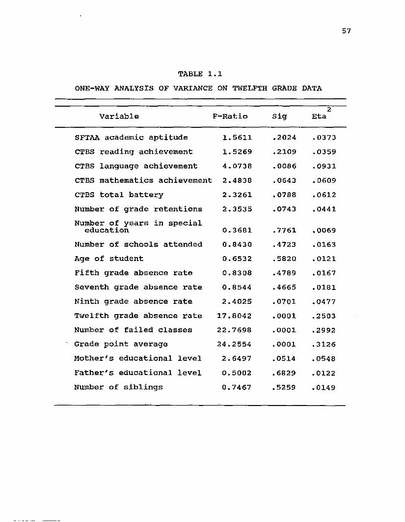
57

TABLE 1.1ONE-WAY ANALYSIS OF VARIANCE ON TWELFTH GRADE DATA

2Variable F-Ratio Sig Eta

SFTAA academic aptitude CTBS reading achievementCTBS language achievementCTBS mathematics achievementCTBS total batteryNumber of grade retentionsNumber of years in special educationNumber of schools attendedAge of studentFifth grade absence rateSeventh grade absence rateNinth grade absence rateTwelfth grade absence rateNumber of failed classesGrade point averageMother's educational levelFather's educational levelNumber of siblings

1.5611 .2024 .03731.5269 .2109 .03594.0738 .0086 .09312.4838 .0643 .06092.3261 .0788 . 06122.3535 .0743 .0441

0.3681 .7761 .00690.8430 .4723 .01630.6532 .5820 .01210.8308 .4789 .01670.8544 .4665 .01812.4025 .0701 .0477

17.8042 .0001 .250322.7698 .0001 .299224.2554 .0001 .31262.6497 .0514 .05480.5002 .6829 . 01220.7467 .5259 . 0149

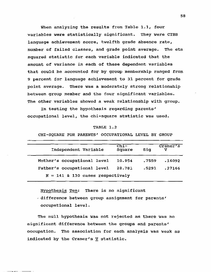
58

When analyzing the results from Table 1.1, four variables were statistically significant. They were CTBS language achievement score, twelfth grade absence rate, number of failed classes, and grade point average. The eta squared statistic for each variable indicated that the amount of variance in each of these dependent variables that could be accounted for by group membership ranged from 9 percent for language achievement to 31 percent for grade point average. There was a moderately strong relationship between group member and the four significant variables.The other variables showed a weak relationship with group.

In testing the hypothesis regarding parents' occupational level, the chi-square statistic was used.

TABLE 1.2CHI-SQUARE FOR PARENTS' OCCUPATIONAL LEVEL BY GROUP

Chi- Cramer'sIndependent Variable Square Sig V

Mother's occupational level 10.954 .7559 .16092Father's occupational level 28.781 .5291 .27166

N = 141 & 130 cases respectively

Hypothesis Ten: There is no significant' difference between group assignment for parents' occupational level.

The null hypothesis was not rejected as there was no significant difference between the groups and parents' occupation. The association for each analysis was weak as indicated by the Cramer's V statistic.

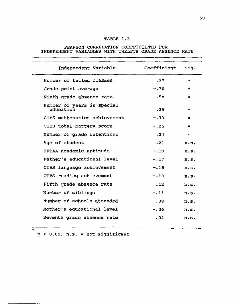
59

TABLE 1.3PEARSON CORRELATION COEFFICIENTS FOR INDEPENDENT VARIABLES WITH TWELFTH GRADE ABSENCE RATE

Independent Variable Coefficient sig.

Number of failed classes .77 *Grade point average -.70 ANinth grade absence rate .58 *Number of years in special education .35 ACTBS mathematics achievement -.33 *CTBS total battery score -.25 *Number of grade retentions .24 *Age of student .21 n.s.SFTAA academic aptitude -.19 n. s.Father's educational level -.17 n.s.CTBS language achievement -.16 n.s.CTBS reading achievement -.13 n.s.Fifth grade absence rate .12 n.s.Number of siblings -.11 n.s.Number of schools attended .08 n.s.Mother's educational level -.06 n.s.Seventh grade absence rate .04 n.s.

*p < 0.05, n.s. = not significant

60

The Pearson product moment correlation coefficients indicated a significant relationship between twelfth grade absence rate and the following variables: number of failedclasses, grade point average, ninth grade absence rate, number of years in special education, CTBS mathematics achievement, CTBS total battery achievement, and the number of grade retentions. Although total battery score and number of grade retentions have a significant relationship with twelfth grade absence rate, the association was weak. Appendix D contains the results for the Pearson correlation coefficients.

When reviewing the other variables' correlation coefficients, the results show that extreme collinearity (.80 and above) exists between number of failed classes with grade point average, reading achievement with total battery, language achievement with total battery, and mathematics achievement with total battery. Grade point average and total battery were not included in the multiple regression analysis because of this situation. Number of failed classes remained because the correlation coefficient was higher for it than for grade point average. CTBS total battery was excluded so that individual subtests could be used to determine whether differences exist among the different achievement areas.

Multiple regression analysis was conducted on the data to determine the best predictors for twelfth grade absence rate without regard to group membership. Inclusion levels were used to force the entry of each variable into the equation. The sequence of variables entered into the equation was determined by the association of the

61

independent variables with the dependent variable, twelfth grade absence rate. Table 1.4 shows the four variables that were entered into the equation and produced significant t values.

TABLE 1.4MULTIPLE REGRESSION ANALYSIS OF THE SIGNIFICANT INDEPENDENT VARIABLES ENTERED IN THE EQUATION

Independent Variable t-Value Sig t

Number of failed classes 6.305 .0001Ninth grade absence rate 3.733 .0004Number of years in special education 2.602 .0116

Seventh grade absence rate -2.151 .0354

Multiple R .85071R square .72370Adjusted R square .65686

DF = 15,62

The forced entry run entered the variables in this order. Number of failed classes accounted for 58 percent of the explained variance of the dependent variable, twelfth grade absence rate, when entered on the first step. Ninth grade absence rate added 5 percent when entered on the second step. Number of years in special education added 1 percent when entered on the third step. Seventh grade absence rate added 2 percent when entered on the

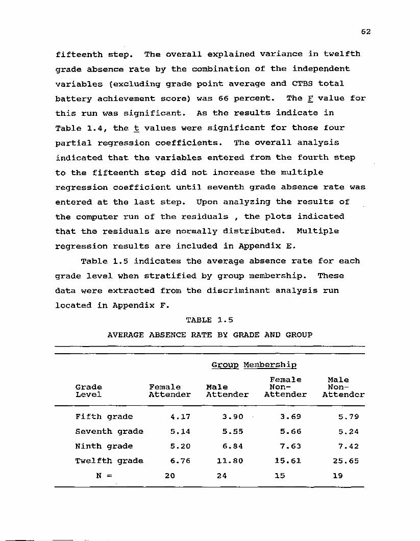
62

fifteenth step. The overall explained variance in twelfth grade absence rate by the combination of the independent variables (excluding grade point average and CTBS total battery achievement score) was 66 percent. The F value for this run was significant. As the results indicate in Table 1.4, the t values were significant for those four partial regression coefficients. The overall analysis indicated that the variables entered from the fourth step to the fifteenth step did not increase the multiple regression coefficient until seventh grade absence rate was entered at the last step. Upon analyzing the results of the computer run of the residuals , the plots indicated that the residuals are normally distributed. Multiple regression results are included in Appendix E.

Table 1.5 indicates the average absence rate for each grade level when stratified by group membership. These data were extracted from the discriminant analysis run located in Appendix F.

TABLE 1.5AVERAGE ABSENCE RATE BY GRADE AND GROUP

Group MembershipFemale MaleGrade Female Male Non- Non-Level Attender Attender Attender Attender

Fifth grade 4.17 3.90 3.69 5.79Seventh grade 5.14 5.55 5.66 5.24Ninth grade 5.20 6.84 7.63 7.42Twelfth grade 6.76 11. 80 15.61 25. 65

N = 20 24 15 19

63

Table 1.5 presents the average absence rate for each group by grade level. With the exception of the female attender group, the average absence rate increased considerably from ninth grade to twelfth grade. Although there was a slight drop from fifth grade to seventh grade for the male non-attenders, there was a steady increase in the average absence rates as students progressed through school. A visual scan of the average ninth grade absence rates indicated that rates tended to differ more by groups at that grade level than in previous years.

Relevant results from the discriminant analysis are provided in the the next five tables. The Wilks' Lambda data are included in Table 1.6 which displays information regarding whether each independent variable was significant in the discriminant function. Table 1.7 provides data on the three canonical discriminant functions which indicate the relative importance of the independent variables in distinguishing between attenders and non-attenders by gender. Standardized canonical discriminant function coefficients are shown in Tables 1.8 and 1.9. These coefficients represent the relative contribution of each variable to the respective functions. Table 2.0 indicates the overall classification matrix with frequencies and percentages of cases included in the analysis that are either correctly or incorrectly classified by discriminant analysis.

The independent variables were analyzed using the Wilks' Lambda statistic which is an inverse measure that determines group discrimination.

64

TABLE 1.6WILKS' LAMBDA DATA FOR TWELFTH GRADE

IndependentVariable

Number of failed classesGrade point averageTwelfth grade absence rateMother's educational levelNumber of schools attendedNumber of siblingsCTBS mathematics achievementCTBS language achievementFather's educational levelNumber of grade retentionsFifth grade absence rateNinth grade absence rateNumber of years in special educationCTBS reading achievementSFTAA academic achievementAge of studentSeventh grade absence rate

DF = 3,74

Wilks' Signif- F-Lambda icance Ratio

,71433 .0001 9.8672102 .0001 9.5473515 .0001 8.8991229 .0772 2 .3791491 . 0849 2.2991987 . 1013 2.1593259 .1578 1.7893854 . 1931 1.6293958 .1999 1.5994337 .2267 1.4895554 . 3356 1.1595873 .3706 1. 06

96569 .4574 0.8896740 .4810 0.8397034 .5235 0.7597692 . 6282 0. 5899778 .9829 0.06

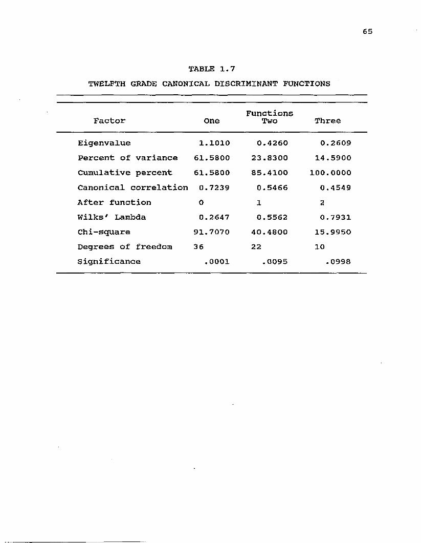
65

TABLE 1.7TWELFTH GRADE CANONICAL DISCRIMINANT FUNCTIONS

Factor One FunctionsTwo Three

Eigenvalue 1.1010 0.4260 0.2609Percent of variance 61.5800 23.8300 14.5900Cumulative percent 61.5800 85.4100 100.0000Canonical correlation 0.7239 0.5466 0.4549After function 0 1 2Wilks' Lambda 0.2647 0.5562 0.7931Chi-square 91.7070 40.4800 15.9950Degrees of freedom 36 22 10Significance .0001 .0095 .0998

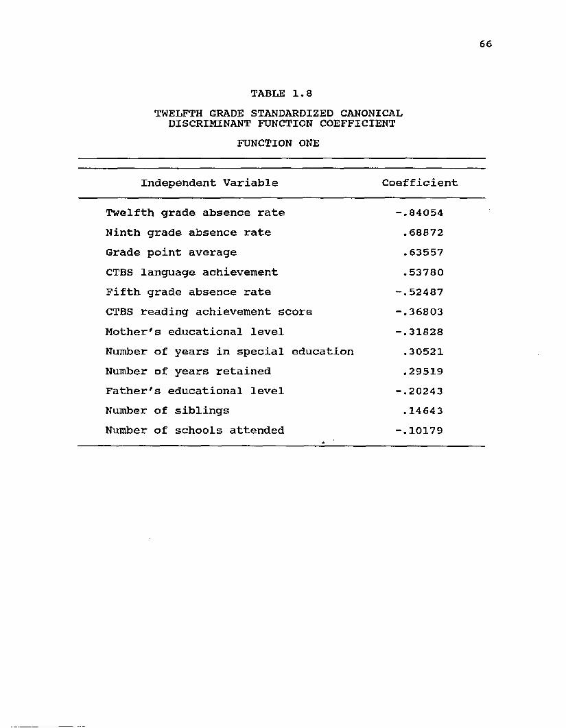
66

TABLE 1.8TWELFTH GRADE STANDARDIZED CANONICAL DISCRIMINANT FUNCTION COEFFICIENT

FUNCTION ONE

Independent Variable Coefficient

Twelfth grade absence rate -.84054Ninth grade absence rate .68872Grade point average .63557CTBS language achievement .53780Fifth grade absence rate -.52487CTBS reading achievement score -.36803Mother's educational level -.31828Number of years in special education .30521Number of years retained .29519Father's educational level -.20243Number of siblings .14643Number of schools attended -.10179

67

TABLE 1.9TWELFTH GRADE STANDARDIZED CANONICAL DISCRIMINANT FUNCTION COEFFICIENTS

FUNCTION TWO

Independent Variable Coefficient

Father's educational level -.99258CTBS reading achievement score .79001Number of years in special education .71347Number of years retained .61100Mother's educational level .48714Number of siblings -.38862Fifth grade absence rate -.32032CTBS language achievement score -.28803Twelfth grade absence rate -.17588Number of schools attended -.16867Grade point average .08257Ninth grade absence rate -.06477

68

TABLE 2.0 TWELFTH GRADE CLASSIFICATION MATRIX

ActualGroups

Predicted Group MembershipFemale Male Female Female Non- Non- Attender Attender Attender Attender

Female attenderFrequency 16 4 3 0Percent 69.6 17.4 13.0 0

Male attenderFrequency 6 15 2 2Percent 24.0 60.0 8 . 0 8.0

Female non-attenderFrequency 3 3 9 4Percent 15.8 15.8 47.4 21.1

Male non-attenderFrequency 1 2 4 15Percent 4.5 9.1 18.2 68.2

N - 23 25 19 22

Groups correctly classified 61.8%

69

The independent variables were ranked by using the Wilks' Lambda statistic (Table 1.6) which is a measure of group discrimination. It determines the significance of the P values in that the variable which has the maximum F-ratio will also have the lowest Lambda value. When reviewing the data, it can be inferred that the number of failed classes, grade point average, and twelfth grade absence rate were major discriminating factors in distinguishing between attenders and non-attenders by gender. The other fourteen variables have F-ratios that were not significant; therefore, they provide little or no discriminatory power in this analysis.

The stepwise procedure of entering variables in the equation was used in this discriminant analysis. This procedure selected the best discriminating variable according to a pre-determined criterion which was the Wilks' Lambda method. Printouts of this procedure are included in Appendix F. During the stepwise procedure, thirteen of the seventeen variables were entered with the number of failed classes being the first independent variable entered into the equation. It was removed at the seventh step as it was found to reduce discrimination when combined with the recent inclusion of other selected variables. Grade point average was entered at the sixth step which probably impacted the "failed classes" variable due to their intercorrelation.

Table 1.7 provides summary information on the discriminant functions. The eigenvalue measures the relative importance of the function; whereas, the sum of the eigenvalues represents the total variance which

70

exists in the discriminating variables. When comparing the eigenvalues for all three functions, the first function contained approximately 62 percent of ^the variance that exists in the discriminating variables with the second function contributing about 23 percent of the variance.The Wilks' Lambda value has been transformed into a chi- square statistic to test statistical significance. Both the first and second functions have a chi-square statistic that was significant. The third function was not significant.

The canonical correlation for each function is a measure of association between the function and the grouping variable. The correlation provides an indication of how well the function discriminates among the four groups. The first function has a strong relationship with the grouping variable; whereas, the second and third functions have a moderately strong relationship. By squaring the canonical correlation, the statistic may be interpreted as the proportion of variance in the dependent variable which can be explained by the collective contributions of the independent variables. Fifty-two percent of the variance within the grouping variable could be explained by the independent variables with the first function. The explained variance in the second function was 30 percent.

Data in Table 1.8 display the standardized canonical discriminant function coefficients for the twelve variables included in the analysis. Each coefficient represents its relative contribution of the variable to the first function. The sign indicates whether the variable

71

contributes positively or negatively to the function. Upon reviewing the coefficients for the first function, twelfth grade absence rate, ninth grade absence rate, grade point average, language achievement, and fifth grade absence rate contributed more importantly than the remaining variables. Twelfth grade absence contributed twice as much as any of the last seven variables in the table.

Results from the second function indicated that the father's educational level, reading achievement, number of years in special education, and number of years retained contribute more than the remainder of the variables. Father's educational level contributed twice as much as the last eight variables (Table 1.8).

Because of the nature of the variables that made the most relative contribution to each function, the first function should be named student absenteeism with the second function entitled achievement. It should be noted that the functions are arranged in order of decreasing importance. A given difference among group means on the second or third function are not as meaningful as the same difference on the first function.

Table 2.0 provides the classification matrix for the twelfth grade data. Of the attenders, 69.6 percent of the females were classified correctly with 60.0 percent of the males correctly classified. Of the non-attenders, 47.4 percent of the females and 68.2 percent of the males were classified correctly. Overall, 61.8 percent of the students were classified correctly. The most frequent misclassification with each group occurred due to gender rather than attendance. For instance, 17.4 percent of the

72

female attenders were misclassified as male attenders; whereas, 13 percent were misclassified as female non- attenders. The results show that female non-attenders were more incorrectly classified than any other group.

In essence, three of the seventeen independent variables were significantly associated with the variation among the groups. The following section provides the testing of the ten hypotheses by using the results from the discriminant analysis procedure.

Hypothesis One: There is no significantdifference between group assignment for academic aptitude.

As indicated by the Wilks' Lambda data in the discriminant analysis, which analyzed the independent variables collectively, and the data from the analysis of variance procedure, which analyzed the independent variables in isolation, the results showed no significant difference. As a result of this situation, the null hypothesis was not rejected.

Hypothesis Two: There is no significantdifference between group assignment for student achievement.

Although the analysis of variance results indicated a significant difference when analyzing language achievement independent of the other variables, the discriminant analysis procedure produced non-significant results when analyzing the independent variables collectively. The null hypothesis was not rejected as the results for the

73

discriminant analysis indicated no significant difference between student achievement in language, mathematics, and reading when compared with group membership.

Hypothesis Three: There is no significantdifference between group assignment for the number of grade retentions.

The Wilks' Lambda data along with the analysis of variance results indicated that there was no significant difference in discriminating between the groups and grade retention; therefore, the null hypothesis was not rejected.

Hypothesis Four: There is no significantdifference between group assignment for the number of years in special education.

Again, both types of analyses indicated no significant difference which resulted in not rejecting the null hypothesis in that the number of years spent in special education did not contribute to discrimination among the groups.

Hypothesis Five: There is no significantdifference between group assignment for the number of schools attended.

There was no evidence of a significant difference between group membership and schools attended as stated in the Wilks' Lambda data; therefore, the null hypothesis was not rejected.

Hypothesis Six: There is no significant

74

difference between group assignment for age.

The null hypothesis was accepted as the results from the discriminant analysis procedure as well as the analysis of variance procedure produced non-significant results.

Hypothesis Seven: There is no significantdifference between group assignment for student absenteeism rate.

This hypothesis was rejected because twelfth grade absence rate did produce significant results with both types of analyses. The absence rate for previous grade levels (fifth, seventh, and ninth) did not produce significant differences between group assignment on an independent basis as indicated by the Wilks' Lambda data, but they did make relative contributions to the first function in distinguishing between the groups which resulted in that function being named student absenteeism.

Hypothesis Eight: There is no significantdifference between group assignment for the number of failed classes in high school.

This hypothesis was rejected due to the number of failed courses being significantly different with group membership. In fact, it was entered on the first step of the discriminant analysis until it was removed when grade point average was entered on the sixth step.

Hypothesis Nine: There is no significantdifference between group assignment for parents' educ at iona1 1eve1.

75

The hypothesis was accepted as both analyses indicated that parents' educational level did not significantly discriminate group membership at the twelfth grade level.

Hypothesis Eleven: There is no significantdifference between group assignment for the number of siblings in the home.

This hypothesis was accepted as the data indicated from both analyses that the number of siblings in the home did not contribute as a discriminating variable for group membership.

As a result of the discriminant analysis, hypotheses seven and eight were rejected as there was a significant difference between group assignment and the students' twelfth grade absence rate as well as the number of failed classes in high school and grade point average.

The other fourteen variables that focused on parents' educational level, retention, special education, schools attended, age, elementary and junior high absence rate, and age were not significant,* therefore, the other eight hypotheses were not rejected as the results could have occurred due to chance.

The multivariate analysis of variance procedure was used to test student satisfaction. Tables 2.1 and 2.2 display the results from this procedure.

Hypothesis Twelve: There is no significantdifference between twelfth grade absence rate and group assignment, twelfth grade absence rate and student satisfaction, and twelfth grade absence rate

76

and group assignment by student satisfaction.

Table 2.1 provides the results from the analysis comparing group assignment with student satisfaction by utilizing the satisfaction scale. One rating, highly dissatisfied, was omitted in the analysis due to the category having empty cells across all groups. Within hypothesis twelve, there were three independent parts. Two parts were to test the main effects of group assignment and student satisfaction with twelfth grade absence rate.Also, there was a test to determine whether there was an interaction effect between group assignment and student satisfaction with twelve grade absence rate.

77

TABLE 2.1TWELFTH GRADE MULTIVARIATE ANALYSIS OF VARIANCE ON TWELFTH GRADE ABSENCE RATE AND STUDENT SATISFACTION

N = 92 cases

Group AssignmentFemale MaleSatisfactionScale FemaleAttender MaleAttender Non-Attender Non-Attender

AlmostDissatisfied 13.60 30.05 43 .73ModeratelySatisfied 6.13 10.20 20.04 22.39AlmostSatisfied 7.50 6.16 14.40 11.10HighlySatisfied 5.75 7.58 11.43 14.66

Analysis of Variance

Source of Variation Sums of Squares MeanD.F. Squares F Sig of F

Within cells 9021.42 78 115 .66Constant 540.76 1 540 .76 4.68 .034Group 1026.28 3 342 .09 2.96 . 037Satisfy 547.43 3 182 .48 1.58 .201Group by Satisfy 458.02 7 65 .43 .57 .782

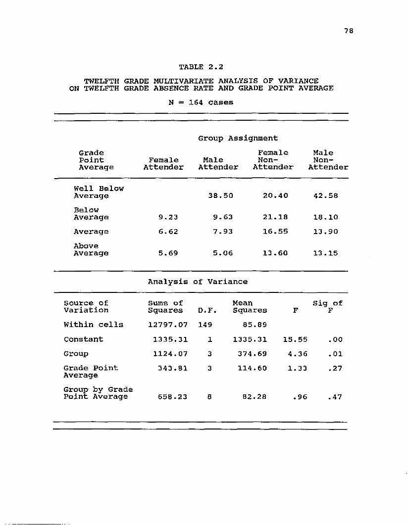
78

TABLE 2.2TWELFTH GRADE MULTIVARIATE ANALYSIS OF VARIANCE ON TWELFTH GRADE ABSENCE RATE AND GRADE POINT AVERAGE

N = 164 cases

Group AssignmentGradePointAverage FemaleAttender

Female Male Non- Attender AttenderMaleNon-Attender

Well Below Average 38.50 20.40 42.58BelowAverage 9.23 9.63 21.18 18.10Average 6.62 7.93 16.55 13.90AboveAverage 5.69 5.06 13.60 13.15

Analysis of Variance

Source of Variation Sums of Squares MeanD.F. Squares F Sig of FWithin cells 12797.07 149 85.89Constant 1335.31 1 1335.31 15.55 , 00Group 1124.07 3 374.69 4.36 . 01Grade Point Average 343.81 3 114.60 1.33 .27

Group by Grade Point Average 658.23 8 82.28 .96 .47

79

Within hypothesis twelve, there were three separate tests of the hypothesis. The first part which tested the main effect of group assignment with twelfth grade absence rate was significant; therefore, that portion of the hypothesis was rejected. The second part which tested the main effect of student satisfaction, as indicated by a derived score between SFTAA academic aptitude score and the CTBS total battery achievement score, was not significant; therefore, the second part of the hypothesis was accepted. The third section of the hypothesis was testing the interaction effect of group assignment by student satisfaction with twelfth grade absence rate. This part of the hypothesis was not significant; therefore, it was accepted. Overall, null hypothesis twelve was accepted as there was no significant difference between group assignment by student satisfaction with twelfth grade absence rate.

Hypothesis Thirteen: There is no significantdifference between twelfth grade absence rate and group assignment, twelfth grade absence rate and grade point average, and twelfth grade absence rate and group assignment by grade point average.

Again, hypothesis thirteen was divided into three parts to test the main effects of group assignment and of grade point average as well as the interaction effect of group assignment by grade point average categories. The main effect of group assignment was significant; whereas, neither the main effect of grade point average categories nor the interaction effect of group assignment and grade

80

point average categories were significant. Because of the lack of a significant interaction effect; the null hypothesis was accepted.

From the results of the multivariate analysis of variance procedure, the data indicated that both hypotheses were to be accepted due to the lack of signficant differences between the interaction of the main effects and twelfth grade absence rate.

Ninth Grade AnalysisThe analyses within this ninth grade section are

presented in the same manner as they were in the twelfth grade section. Appendix H includes the student data file for ninth grade. The results of the one-way analysis of variance for each variable are displayed in Table 2.3. Appendix I contains the results from this procedure. Parents' occupational level by group assignment is contained in Table 2.4 with the results from the chi-square statistic being included in Appendix J. The Pearson product moment correlation coefficients are included in Table 2.5 while the results from that procedure can be located in Appendix K.

81

TABLE 2.3ONE-WAY ANALYSIS OF VARIANCE ON NINTH GRADE DATA

Variable F-Ratio Sig 2Eta

TCS academic aptitude 2.3388 .0777 .0621CTBS reading achievement 6.5059 .0004 .1440CTBS language achievement 10.7938 .0001 .2153CTBS math achievement 7.0940 . 0002 .1562CTBS total battery 8.7267 .0001 .1951Number of years retained 2.5557 .0574 .0477Number of years in special education 1.7548 .1580 .0317Number of schools attended 5.5475 .0012 .0993Age of student 6.7147 . 0003 . 1106Fifth grade absence rate 3.7533 . 0124 .0740Seventh grade absence rate 16.1400 .0001 .2640Ninth grade absence rate 63.0486 . 0001 .5387Number of failed classes 34.8383 . 0001 . 3922Grade point average 61.7402 .0001 . 5334Mother's educational level 2.6011 .0548 .0554Father's educational level 3.2389 .0247 . 0773Number of siblings .7153 .5443 . 0143

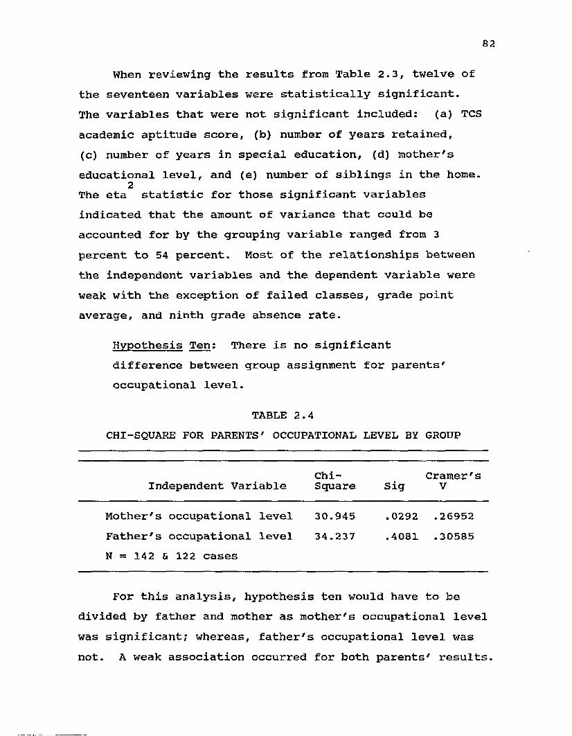
82

When reviewing the results from Table 2.3, twelve ofthe seventeen variables were statistically significant.The variables that were not significant included: (a) TCSacademic aptitude score, (b) number of years retained,(c) number of years in special education, (d) mother'seducational level, and (e) number of siblings in the home.

2The eta statistic for those significant variables indicated that the amount of variance that could be accounted for by the grouping variable ranged from 3 percent to 54 percent. Most of the relationships between the independent variables and the dependent variable were weak with the exception of failed classes, grade point average, and ninth grade absence rate.

Hypothesis Ten: There is no significantdifference between group assignment for parents' occupational level.

TABLE 2.4CHI-SQUARE FOR PARENTS' OCCUPATIONAL LEVEL BY GROUP

Independent Variable Chi-Square Sig Cramer's V

Mother's occupational level 30.945 .0292 .26952Father's occupational level N = 142 6 122 cases

34.237 .4081 .30585

For this analysis, hypothesis ten would have to be divided by father and mother as mother's occupational level was significant? whereas, father's occupational level was not. A weak association occurred for both parents' results.

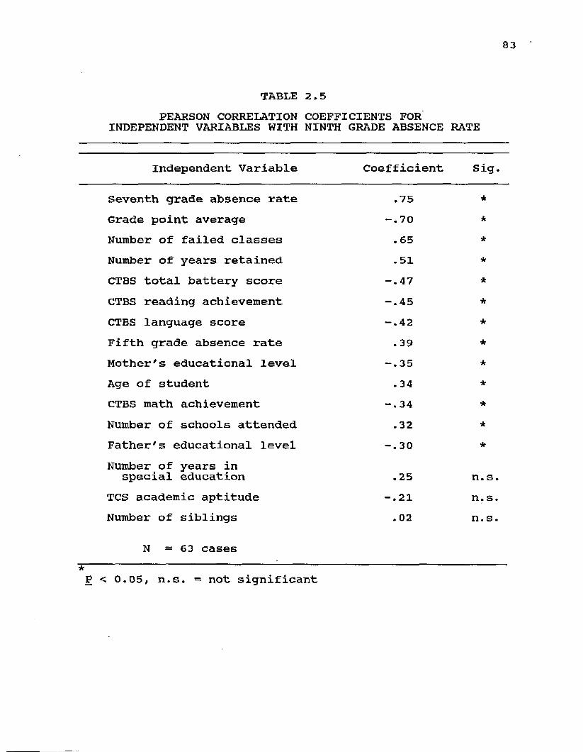
83

TABLE 2.5PEARSON CORRELATION INDEPENDENT VARIABLES WITH COEFFICIENTS FOR NINTH GRADE ABSENCE RATE

Independent Variable Coefficient Sig.

Seventh grade absence rate .75 *Grade point average -.70 *Number of failed classes .65 *

Number of years retained .51 *CTBS total battery score -.47 *CTBS reading achievement -.45 *CTBS language score -.42 *Fifth grade absence rate .39 *Mother's educational level -.35 *

Age of student . 34 *CTBS math achievement -.34 *Number of schools attended .32 *Father's educational level -.30 *Number of years in special education .25 n.s.TCS academic aptitude -.21 n.s.Number of siblings . 02 n.s.

N = 6 3 cases*P < 0.05, n.s. = not significant

84

With the exception of three variables: number ofyears in special education, TCS academic aptitude score, and number of siblings in the home; all the Pearson correlation coefficients indicated a significant relationship with ninth grade absence rate. Most of the relationships between the significant variables and ninth grade absence rate were moderately strong. Seventh grade absence rate, grade point average, and number of failed classes exhibited a strong relationship with ninth grade absence rate.

When reviewing the other variables' correlation coefficients, the results showed extreme collinearity (.80 and above) between CTBS total battery achievement and the three subtests as well as TCS academic aptitude. CTBS total battery achievement score and the number of failed classes' variables were omitted from the multiple regression analysis due to their intercorrelation with the other variables.

Multiple regression analysis was conducted on the data to determine the best predictors for ninth grade absence rate without regard to group membership. Inclusion levels were used to force the entry of each variable into the equation. The sequence of the entered variables was determined by the Pearson correlation coefficients of the independent variables with the dependent variable, ninth grade absence rate. Table 2.6 shows the four variables that were entered into the equation and produced t values that were significant.

85

TABLE 2.6MULTIPLE REGRESSION ANALYSIS OF THE SIGNIFICANT INDEPENDENT VARIABLES ENTERED IN THE EQUATION

Independent Variable t-Value Sig t

Seventh grade absence rate 4.208 .0001Grade point average - 3.121 .0031Number of years retained 2.970 .0046CTBS reading achievement - 3.187 .0025

Multiple R .88942R square .79106Adjusted R square .73013

DF = 14,48

The forced entry run included seventh grade absence rate on the first step. This variable accounted for 56 percent of the explained variance of ninth grade absence rate. When grade point average was entered into the equation on the second step, it added 9 percent to the explained variance. Number of years retained was added on the third step and added 3 percent to the explained variance. When CTBS reading achievement was entered on the fourth step, it added 1 percent to the explained variance. The overall explained variance in ninth grade absence rate by the collective contributions of the independent variables (excluding number of failed classes and CTBS

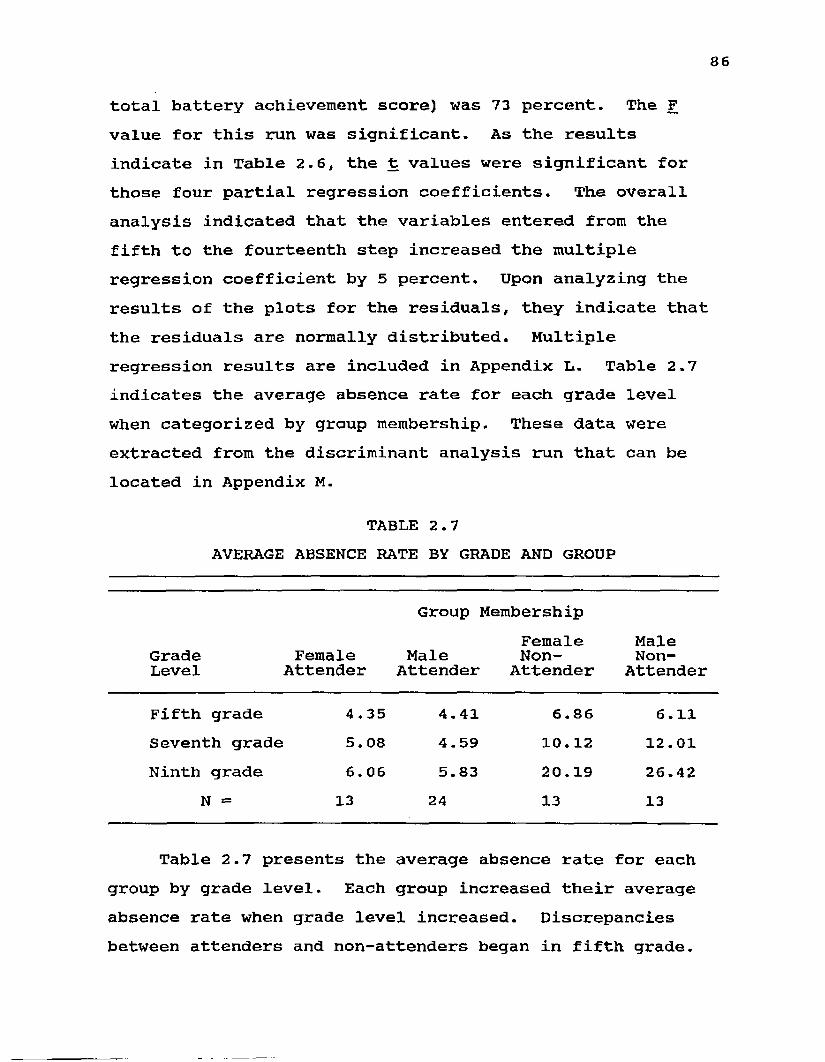
86

total battery achievement score) was 73 percent. The F value for this run was significant. As the results indicate in Table 2.6, the t values were significant for those four partial regression coefficients. The overall analysis indicated that the variables entered from the fifth to the fourteenth step increased the multiple regression coefficient by 5 percent. Upon analyzing the results of the plots for the residuals, they indicate that the residuals are normally distributed. Multiple regression results are included in Appendix L. Table 2.7 indicates the average absence rate for each grade level when categorized by group membership. These data were extracted from the discriminant analysis run that can be located in Appendix M.

TABLE 2.7AVERAGE ABSENCE RATE BY GRADE AND GROUP

Group MembershipFemale MaleGrade Female Male Non- Non-Level Attender Attender Attender Attender

Fifth grade 4.35 4.41 6.86 6..11Seventh grade 5.08 4.59 10.12 12..01Ninth grade 6.06 5.83 20.19 26..42

N = 13 24 13 13

Table 2.7 presents the average absence rate for each group by grade level. Each group increased their average absence rate when grade level increased. Discrepancies between attenders and non-attenders began in fifth grade.

87

Discriminant analysis results are outlined in the next four tables. The Wilks7 Lambda data are included in Table 2.8 with Table 2.9 containing the canonical discriminant functions. Table 3.0 displays the standardized canonical discriminant function coefficients for function one as the other two functions were not significant. Table 3.1 provides the overall classification matrix with frequencies and percentages of cases included in the analysis that are either classified correctly or incorrectly by discriminant analysis.

The ten hypotheses that were discussed in the twelfth grade section in regards to discriminant analysis were also tested in this section. There were sixteen variables included in the discriminant analysis procedure. Again, the stepwise procedure of entering variables into the equation was used. Printouts of this analysis are included in Appendix M.

During this procedure eight of the sixteen variables were entered into the equation with ninth grade absence rate entered on the first step, the number of failed classes was entered on the second step. The TCS academic aptitude score was entered on the third step with CTBS language achievement entered on the fourth step. Number of siblings in the home was entered on the fifth step; whereas, mother7s educational level was the sixth variable entered into the equation. CTBS mathematics achievement was the seventh step variable with grade point average being entered on the eighth and final step of the equation.

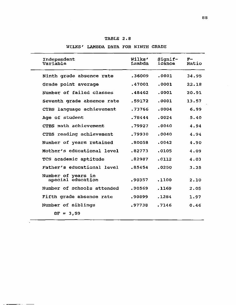
88

TABLE 2.8WILKS' LAMBDA DATA FOR NINTH GRADE

IndependentVariable Wilks'Lambda Signif­icance F-Ratio

Ninth grade absence rate .36009 . 0001 34.95Grade point average .47001 .0001 22.18Number of failed classes .48462 .0001 20.91Seventh grade absence rate .59172 . 0001 13.57CTBS language achievement .73766 .0004 6.99Age of student .78444 .0024 5.40CTBS math achievement .79927 .0040 4 . 94CTBS reading achievement .79930 . 0040 4.94Number of years retained .80058 .0042 4 .90Mother's educational level .82773 .0105 4.09TCS academic aptitude .82987 .0112 4.03Father's educational level .85454 .0250 3 . 35Number of years in special education .90357 .1100 2.10Number of schools attended .90569 .1169 2 . 05Fifth grade absence rate .90899 .1284 1.97Number of siblings .97738 .7146 0.46

DF = 3,59

89

TABLE 2.9NINTH GRADE CANONICAL DISCRIMINANT FUNCTIONS

Factor One FunctionsTwo Three

Eigenvalue 3.0849 0.2526 0.1299Percent of variance 88.9700 7.2900 3 .7500Cumulative percent 88.9700 96.2500 100.0000Canonical correlation .8690 .4491 .3391After function 0 1 2Wilks' Lambda . 1730 .7066 .8850Chi-square 98.2610 19.4520 6.8390Degrees of freedom 24 14 6Significance .0001 .1484 .3360

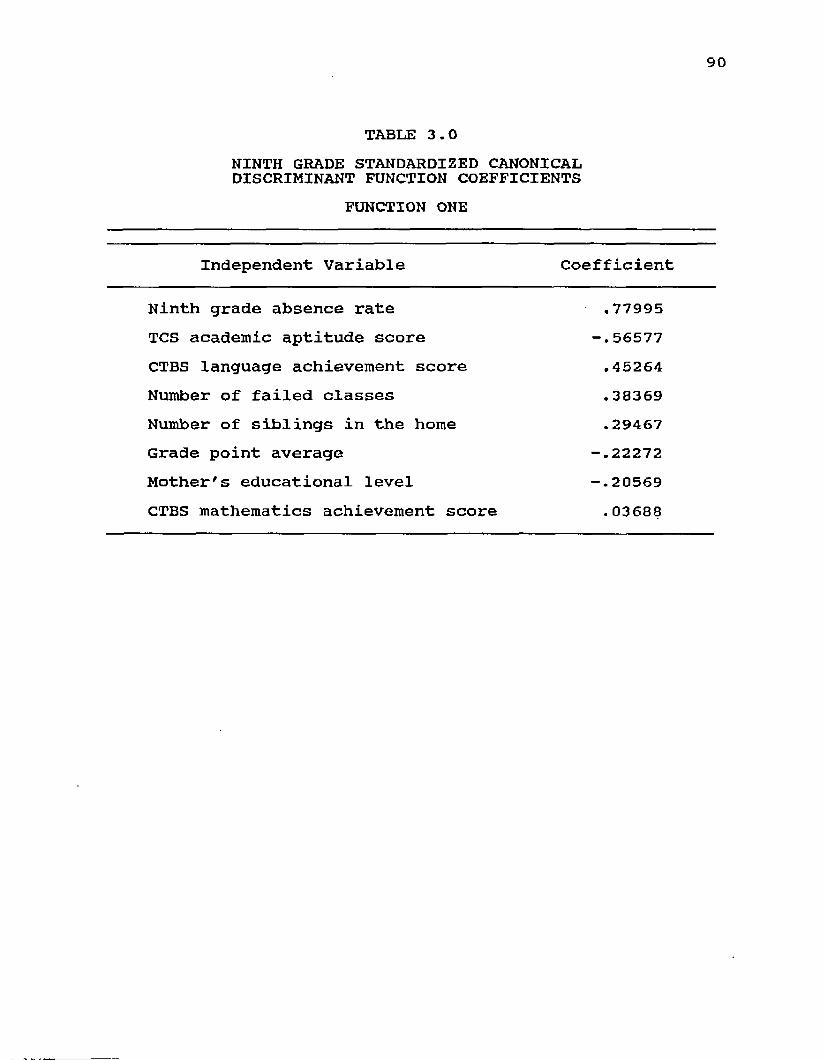
90

TABLE 3.0NINTH GRADE STANDARDIZED CANONICAL DISCRIMINANT FUNCTION COEFFICIENTS

FUNCTION ONE

Independent Variable Coefficient

Ninth grade absence rate ,77995TCS academic aptitude score -.56577CTBS language achievement score .45264Number of failed classes .38369Number of siblings in the home .29467Grade point average -.22272Mother's educational level -.20569CTBS mathematics achievement score .03688

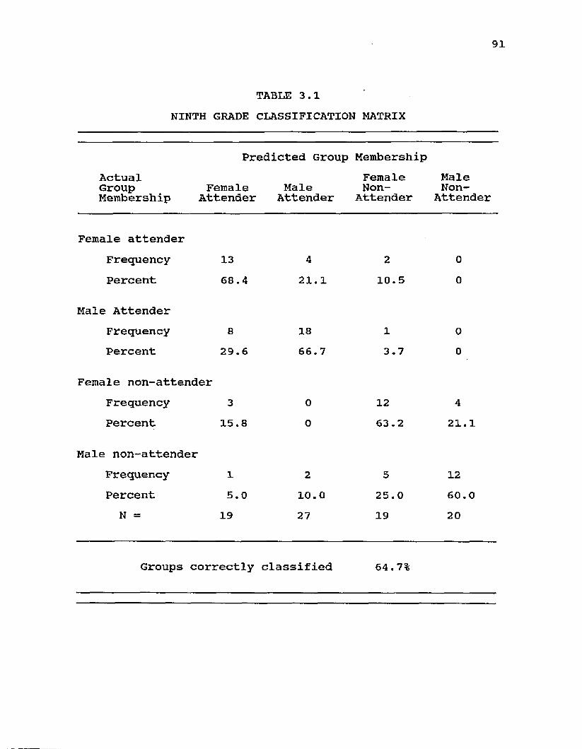
91

TABLE 3.1 NINTH GRADE CLASSIFICATION MATRIX

Predicted Group MembershipActualGroupMembership FemaleAttender MaleAttender

FemaleNon-AttenderMaleNon-Attender

Female attenderFrequency 13 4 2 0Percent 68.4 21.1 10. 5 0

Male AttenderFrequency 8 18 1 0Percent 29.6 66.7 3.7 0

Female non-attenderFrequency 3 0 12 4Percent 15.8 0 63.2 21.1

Male non-attenderFrequency 1 2 5 12Percent 5.0 10.0 25.0 60.0N = 19 27 19 20

Groups correctly classified 64.7%

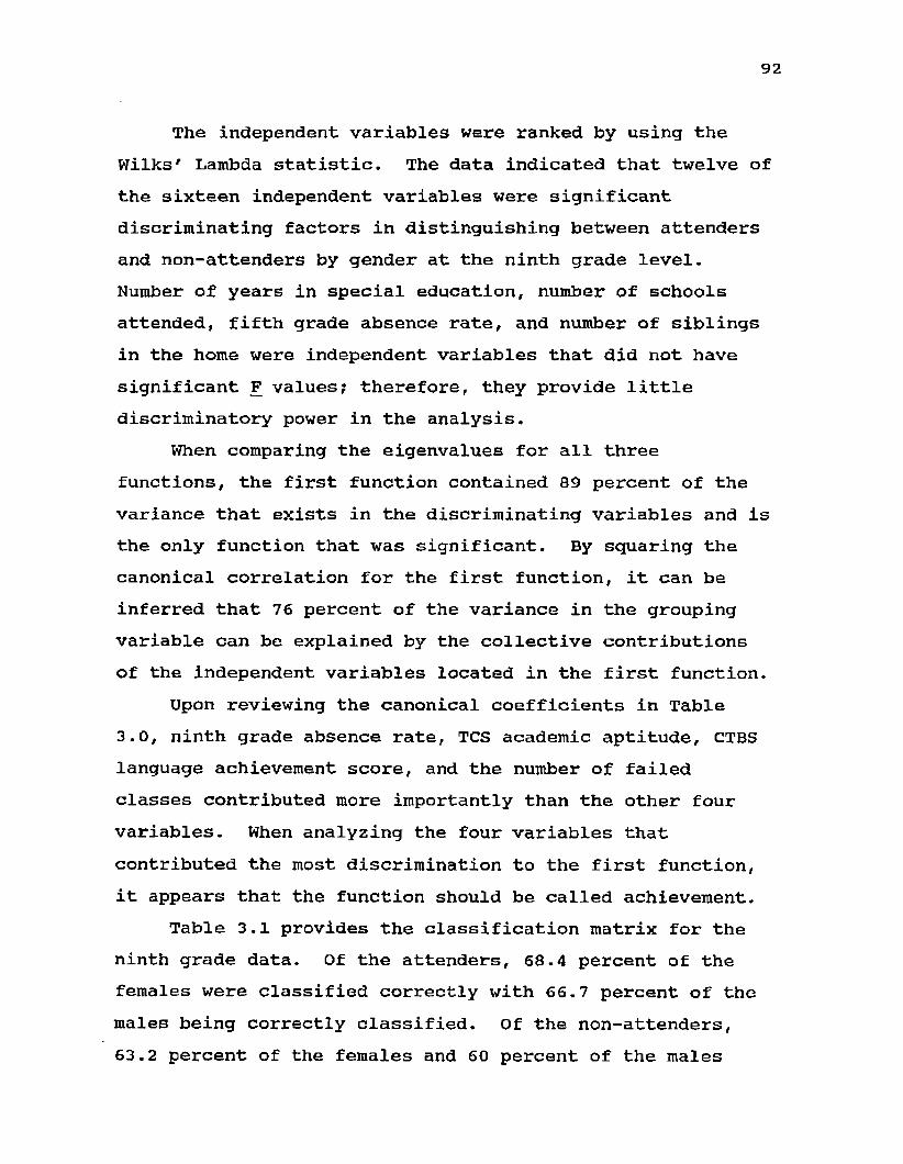
92

The independent variables were ranked by using the Wilks' Lambda statistic. The data indicated that twelve of the sixteen independent variables were significant discriminating factors in distinguishing between attenders and non-attenders by gender at the ninth grade level.Number of years in special education, number of schools attended, fifth grade absence rate, and number of siblings in the home were independent variables that did not have significant F values; therefore, they provide little discriminatory power in the analysis.

When comparing the eigenvalues for all three functions, the first function contained 89 percent of the variance that exists in the discriminating variables and is the only function that was significant. By squaring the canonical correlation for the first function, it can be inferred that 76 percent of the variance in the grouping variable can be explained by the collective contributions of the independent variables located in the first function.

Upon reviewing the canonical coefficients in Table 3.0, ninth grade absence rate, TCS academic aptitude, CTBS language achievement score, and the number of failed classes contributed more importantly than the other four variables. When analyzing the four variables that contributed the most discrimination to the first function, it appears that the function should be called achievement.

Table 3.1 provides the classification matrix for the ninth grade data. Of the attenders, 68.4 percent of the females were classified correctly with 66.7 percent of the males being correctly classified. Of the non-attenders,63.2 percent of the females and 60 percent of the males

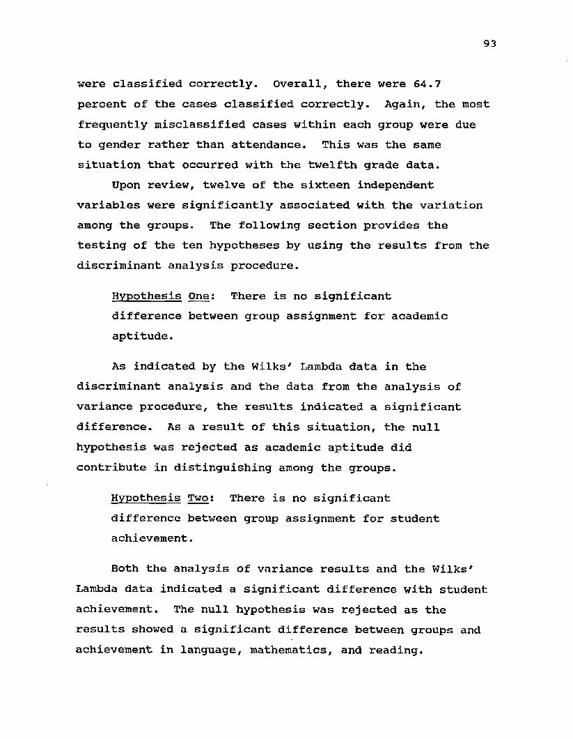
93

were classified correctly. Overall, there were 64.7 percent of the cases classified correctly. Again, the most frequently misclassified cases within each group were due to gender rather than attendance. This was the same situation that occurred with the twelfth grade data.

Upon review, twelve of the sixteen independent variables were significantly associated with the variation among the groups. The following section provides the testing of the ten hypotheses by using the results from the discriminant analysis procedure.

Hypothesis One: There is no significantdifference between group assignment for academic aptitude.

As indicated by the Wilks' Lambda data in the discriminant analysis and the data from the analysis of variance procedure, the results indicated a significant difference. As a result of this situation, the null hypothesis was rejected as academic aptitude did contribute in distinguishing among the groups.

Hypothesis Two: There is no significantdifference between group assignment for student achievement.

Both the analysis of variance results and the Wilks' Lambda data indicated a significant difference with student achievement. The null hypothesis was rejected as the results showed a significant difference between groups and achievement in language, mathematics, and reading.

94

Hypothesis Three: There is no significantdifference between group assignment for the number of grade retentions.

The Wilks' Lambda data indicated a significant difference when the variable was analyzed collectively with the other fifteen variables in discriminating among the groups; therefore, the null hypothesis was rejected.

Hypothesis Four; There is no significant difference between group assignment for the number of years in special education.

Both types of analyses indicated that there was no significant difference which results in accepting the null hypothesis in that the number of years in special education does not contribute significantly in distinguishing among the groups.

Hypothesis Five: There is no significantdifference between group assignment for the number of schools attended.

There was no evidence that there was a significant difference as stated in the Wilks' Lambda data; therefore, the null hypothesis was accepted. The number of schools that a student attends did not assist in significantly discriminating between attenders and non-attenders by gender.

Hypothesis Six: There is no significantdifference between group assignment for age.

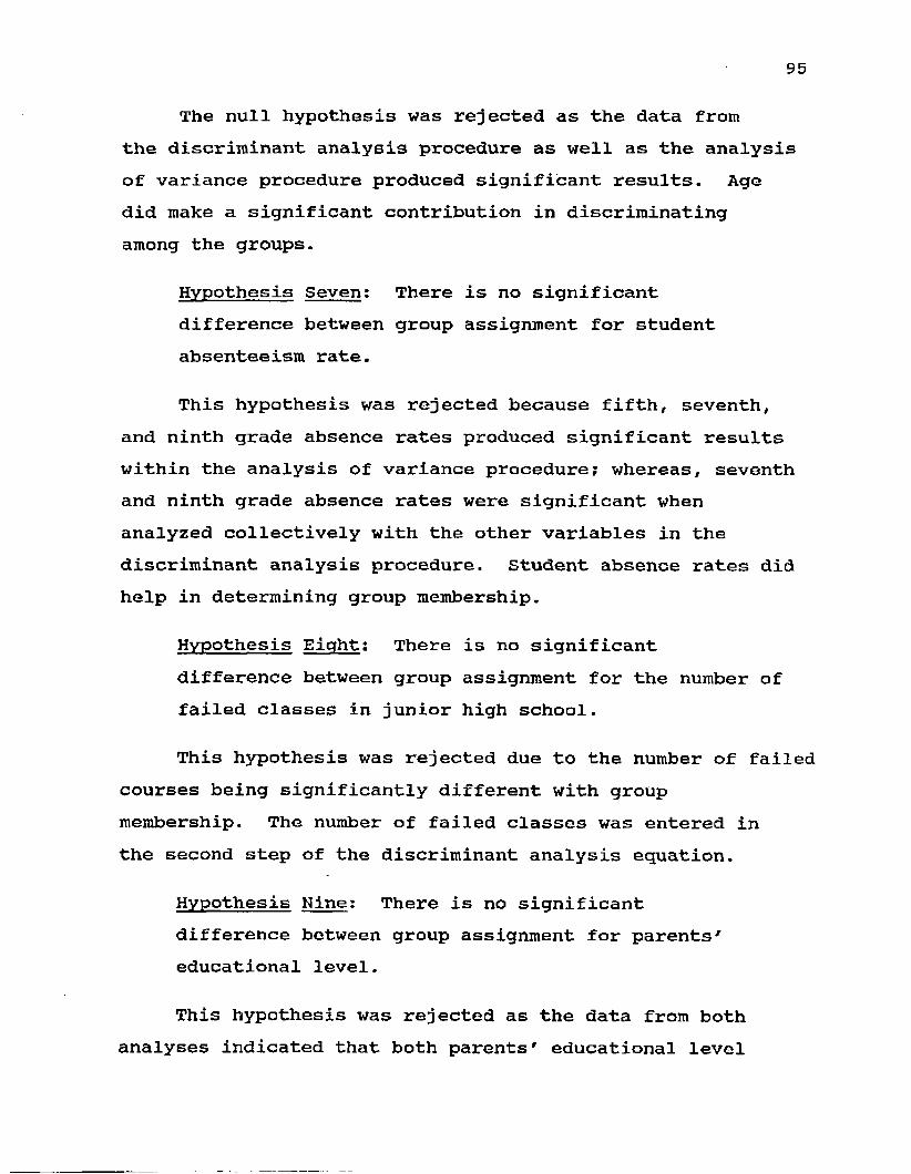
95

The null hypothesis was rejected as the data from the discriminant analysis procedure as well as the analysis of variance procedure produced significant results. Age did make a significant contribution in discriminating among the groups.

Hypothesis Seven: There is no significantdifference between group assignment for student absenteeism rate.

This hypothesis was rejected because fifth, seventh, and ninth grade absence rates produced significant results within the analysis of variance procedure; whereas, seventh and ninth grade absence rates were significant when analyzed collectively with the other variables in the discriminant analysis procedure. Student absence rates did help in determining group membership.

Hypothesis Eight: There is no significantdifference between group assignment for the number of failed classes in junior high school.

This hypothesis was rejected due to the number of failed courses being significantly different with group membership. The number of failed classes was entered in the second step of the discriminant analysis equation.

Hypothesis Nine: There is no significantdifference between group assignment for parents' educational level.

This hypothesis was rejected as the data from both analyses indicated that both parents' educational level

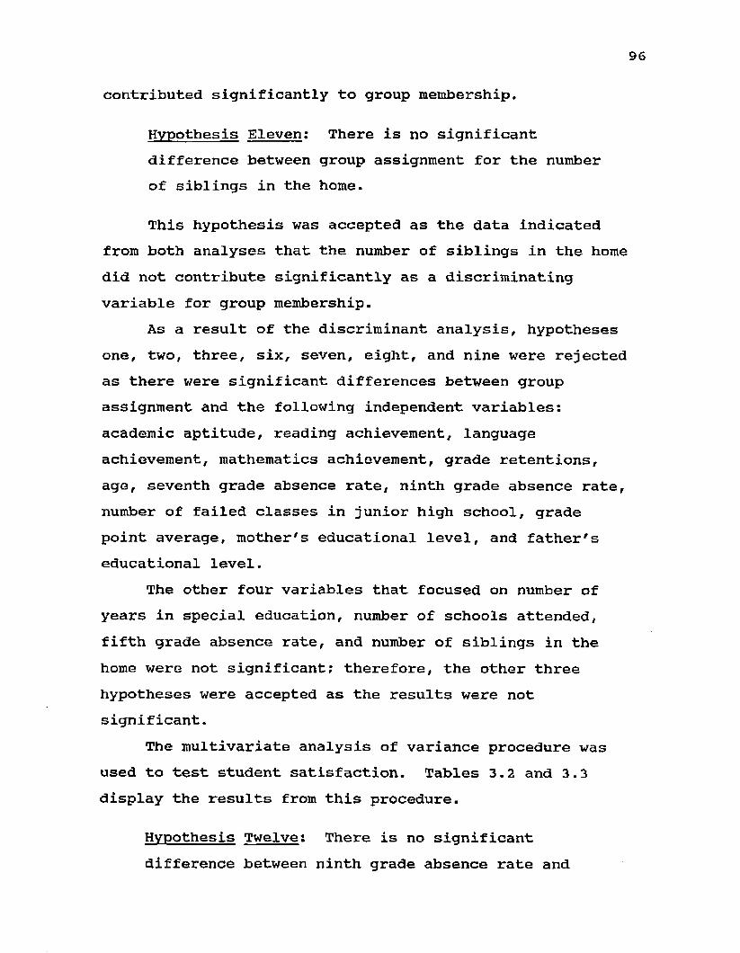
96

contributed significantly to group membership.

Hypothesis Eleven: There is no significantdifference between group assignment for the number of siblings in the home.

This hypothesis was accepted as the data indicated from both analyses that the number of siblings in the home did not contribute significantly as a discriminating variable for group membership.

As a result of the discriminant analysis, hypotheses one, two, three, six, seven, eight, and nine were rejected as there were significant differences between group assignment and the following independent variables: academic aptitude, reading achievement, language achievement, mathematics achievement, grade retentions, age, seventh grade absence rate, ninth grade absence rate, number of failed classes in junior high school, grade point average, mother's educational level, and father's educational level.

The other four variables that focused on number of years in special education, number of schools attended, fifth grade absence rate, and number of siblings in the home were not significant; therefore, the other three hypotheses were accepted as the results were not significant.

The multivariate analysis of variance procedure was used to test student satisfaction. Tables 3.2 and 3.3 display the results from this procedure.

Hypothesis Twelve: There is no significantdifference between ninth grade absence rate and

97

group assignment, ninth grade absence rate and student satisfaction, and ninth grade absence rate and group assignment by student satisfaction.

Table 3.2 provides the results from the analysis comparing group assignment with student satisfaction by utilizing the satisfaction scale. One rating, highly dissatisfied, was omitted due to the category having empty cells. Within hypothesis twelve, there were three separate tests which tested the main effects and the interaction effect of group assignment and student satisfaction with ninth grade absence rate.

98

TABLE 3.2NINTH GRADE MULTIVARIATE ANALYSIS OF VARIANCE ON NINTH GRADE ABSENCE RATE AND STUDENT SATISFACTION

N = 80 cases

Group Assignment

SatisfactionScale FemaleAttender MaleAttenderFemaleNon-Attender

MaleNon-Attender

AlmostDissatisfied 7.77 3.70 16.90 24.25ModeratelySatisfied 5.85 5.49 24.35 21.09AlmostSatisfied 5.37 4.67 22.40HighlySatisfied 4.02 7.25 20.60

Analysis of Variance

Source of Variation Sums of Squares MeanD.F. Squares F Sig of F

Within cells 2878.14 71 40.54Constant 771.67 1 771.67 19.04 .001Group 2476.15 3 825.38 20.36 .001Satisfy 73.43 3 24.48 . 60 . 615Group by Satisfy 209.87 7 29.98 .74 . 639

99

TABLE 3.3NINTH GRADE MULTIVARIATE ANALYSIS OF VARIANCE ON NINTH GRADE ABSENCE RATE AND GRADE POINT AVERAGE

N = 166 cases

Group AssignmentGradePointAverage FemaleAttender

Female Male Non- Attender AttenderMaleNon-Attender

Well Below Average 9.00 9.70 28.94 29.48BelowAverage 7.72 7.44 19.69 19.65Average 6.36 6.00 17.60AboveAverage 5.22 4.17

Analysis of Variance

Source of Variation Sums of Squares MeanD.F. Squares F Sig of FWithin cells 10790.14 153 70.52Constant 558.75 1 558.75 7.92 . 006Group 1337.81 3 445.94 6.32 . 001Grade Point Average 491.10 3 163.70 2.32 . 077Group by Grade Point Average 260.85 6 43.47 .62 . 717

100

Within hypothesis twelve, there were three separate tests of the hypothesis. The first part which tested the main effect of group assignment with ninth grade absence rate was significant; therefore, that portion of the hypothesis was rejected. The second part which tested the main effect of student satisfaction, as indicated by a derived score between TCS academic aptitude score and the CTBS total battery achievement score, was not significant; therefore, the second part of the hypothesis was accepted. The third section of the hypothesis tested the interaction effect of group assignment by student satisfaction with ninth grade absence rate. This part of the hypothesis was not significant; therefore, it was accepted. Overall, the null hypothesis twelve was accepted as there was no significant difference between group assignment by student satisfaction with ninth grade absence rate.

Hypothesis Thirteen: There is no significantdifference between ninth grade absence rate and group assignment, ninth grade absence rate and grade point average, and ninth grade absence rate and group assignment by grade point average.

Again, hypothesis thirteen was divided into three parts to test the main effects of group assignment and of grade point average as well as the interaction effect of group assignment by grade point average categories. The main effect of group assignment was significant; whereas, the main effect of grade point average categories and the interaction effect of group assignment and grade point average categories were not significant. Because of the

101

lack of a significant interaction effect; the null hypothesis was accepted.

From the results of the multivariate analysis of variance procedure, the data indicated that both hypotheses were to be accepted due to the lack of signficance between the interaction of the main effects with the ninth grade absence rate.

SummaryNinth grade results indicated that twelve independent

variables contributed significantly to the discrimination among the groups. Only one function within the ninth grade analysis was significant. The function was named achievement due to its major contribution to the discrimination between attenders and non-attenders by gender. Within the achievement function, 76 percent of the variance in the grouping variable could be explained by the collective contributions of the independent variables within the significant function. Also, 65 percent of the students were classified correctly with most misclassifications occurring due to gender rather than attendance.

Twelfth grade results did not produce as many variables that contributed significantly to the discrimination among the groups. Although two functions were significant, only four variables made significant contributions. Student absenteeism and achievement contributed to distinguishing among the groups. Approximately 52 percent of the variance in the grouping variable could be accounted for by the collective contributions of the independent variables in the first

102

function entitled student absenteeism. Within the second function, 30 percent could be explained by the contributions of the independent variables to the grouping variable. The second function was entitled achievement due to the relative importance of the achievement variables within that function. Approximately 62 percent of the twelfth grade students were classified correctly with the same situation holding true for misclassifications as with the ninth grade students.

Overall, the results indicated that 52 percent of the variance in the grouping variable can be accounted for by the collective contributions of the independent variables in the first function for the twelfth grade analysis. The ninth grade results indicated that the variance in the grouping variable that could be accounted for by the collective contributions of the independent variables within the first function was 76 percent.

CHAPTER V

CONCLUSIONS AND RECOMMENDATIONS

Introduct ionThe primary purpose of this study was to determine

whether group differences occurred between those students who attended school on a regular basis and those students who did not. Specifically, the study focused on developing a profile of a twelfth grade non-attender within a suburban school district by analyzing several variables simultaneously. In addition, this analysis was replicated at the ninth grade level to determine whether the same variables that surfaced at the twelfth grade would collectively contribute to identifying a non-attender at the ninth grade. The last objective of the study centered on whether or not student satisfaction had a bearing on school attendance with regard to gender.

This chapter includes a discussion of the study's conclusions, its limitations, and the recommendations for the subject school district as well as future implications for research studies.

ConclusionsThe discriminant analysis procedure provided valuable

information in identifying those variables that collectively contribute in distinguishing attenders from non-attenders by gender at both the ninth and the twelfth grade levels. The findings indicate that data can be

103

104

obtained readily from students' cumulative records to predict attenders from non-attenders at both grade levels.

In determining attenders from non-attenders when stratifying the groups by gender, similar discriminating variables occurred at both grade levels. There were more contributing factors at the ninth grade level than at the twelfth grade level. The amount of variance within the grouping variable (attenders and non-attenders by gender) at the ninth grade level was 76 percent; whereas, the amount at the twelfth grade level was 52 percent. The findings from the first discriminant function for both grades showed:

(a) Current grade level absence rate assisted in discriminating between attenders and non-attenders by gender.

(b) Grade point average contributed toward distinguishing among the groups.

(c) Language achievement had a significant contribution in determining group differences by gender.

(d) Number of siblings residing in the home provided little discriminatory power at either grade levels.

(e) Mother's educational level also contributed collectively in distinguishing among the groups.

While academic aptitude was not a significant factor

105

in discriminating among the groups at the twelfth grade level, it was a significant contributor at the ninth grade level. Mathematics achievement was a contributing factor at the ninth grade level along with the number of failed classes, which had been removed from the discriminant analysis procedure at the twelfth grade level due to its diminishing discriminatory power after grade point average had been entered. More independent variables at the ninth grade level were significant in the discriminant analysis than at the twelfth grade level for the same procedure.

From the findings it can be concluded that the male non-attender profile contains the following attributes.

(a) has a lower academic aptitude;

(b) achieves significantly lower than females in language-related activities;

(c) achieves lower than females on related mathematical skills;

(d) has a higher absence rate at the current grade level than female non-attenders;

(e) has failed almost twice as many classes as female non-attenders;

(f) possesses a lower grade point average than females;

(g) has a mother who completed more education than female non-attenders' mothers;

106

(h) has less siblings residing in the home than female non-attenders.

Language achievement plays a more important role in the profile at the junior high school level than at the high school level. This deficiency between males and females is much greater at junior high than at high school. When academic aptitude and achievement were combined to analyze student satisfaction in attending school, the interaction with the students' current grade absence rate by group was not significantly different. There was usually a steady decline from the almost dissatisfied category to the highly satisfied category with current grade level absence rate regardless of group assignment.

LimitationsThe conclusions of this study were limited in several

ways. When conducting the data collection procedures, it became evident that data were missing from student records at both grade levels. Once the analyses were conducted on the data, particularly with the discriminant analysis procedure; it became evident that many cases were excluded due to missing data on at least one variable. Test scores tended to be the most prevalent score missing. In addition, the number of disciplinary contacts variable was to have been included in this study but had to be excluded for two reasons: School District personnel lost data fileand inconsistent data collection procedures conducted at the secondary buildings.

RecommendationsTwo recommendations are suggested due to the data

107

presented in the previous chapter and the conclusions from this chapter. The first recommendation focuses on the role of the subject school district in identifying and assisting students with attendance problems prior to entering the secondary schools; whereas, the second recommendation pertains to the replication of this study.

Information obtained from this study could have a valuable effect on the administrative decision-making procedures with the subject school district. Since language achievement had a significant contribution in discriminating between male and female non-attenders, it should be considered a criterion for identifying potential non-attenders in the early elementary level. In addition, absence rate was also a strong contributor; therefore, at least a five percent absence rate should be used as a criterion for early identification of chronic absentees.

It may be advantageous to track students who possess the characteristics set forth in the non-attender profile to ensure that these students are provided assistance prior to junior high so that the probability of those students exhibiting attendance problems at the secondary level can be decreased.

For additional research on absenteeism as it pertains to the non-attender profile, language achievement should be further analyzed to identify specific skill deficiencies in language arts. Furthermore, future research topics could include the study of the effects of an experimental language arts program in reducing student absenteeism in either the junior high or middle school level when compared to a traditional language arts program.

108

It is suggested that if this study is replicated, the research omit the stratification of groups by gender and divide only on attendance. Also, student satisfaction should be further analyzed using language achievement rather than total battery achievement when combined with academic aptitude. In addition, the analysis could be conducted at the early elementary level to see if the results remain non-significant or if there is a difference between student absence rates among the groups when academic aptitude and total battery achievement are combined.

APPENDICES

109

APPENDIX A TWELFTH GRADE STUDENT DATA

110

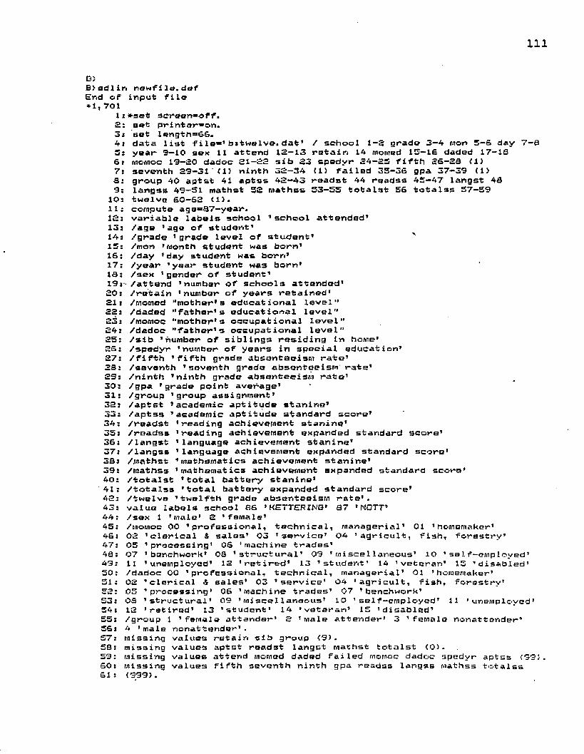
I l l

0}Bledlin rtawf ilo. daf End of input file *1, 701

11 *sat 3m*eon»off.2: sat printarnon.3; set Iength=66,j data list f i la*’ bitwelve. d a f / school 1-3 grade 3—4 mart 5—6 day 7—a

5: year 3— 10 sex 11 attend 12— 13 retain 14 mowed 15— 16 daded 17— IS6i mornoc 19—30 dadoc 21—32 sib 23 spadyr £4—25 fifth 26-28 (1)7; seventh £3—31 11) ninth 32—34 Cl) failed 35—36 gpa 37—33 (1)St group 40 aptst 41 aptss 42—43 readst 44 readss 45-47 langst 483: langss 49—51 mathst 52 mathss 53—55 totalst 56 tota las 57—59

10: twelve 60—62 (1>.111 compute age**B7—year.12: variable labels school ''school attended'13: /age ’age of student'14s /grade ’grade level of student* y15: /mon 'month student was born’16: /day 'day student was born’17: /year 'year student was born’18: /sex 1 gender of student’13: - /attend ’number of schools attended'20: /retain 'number of years retained’21; /niODiad "mother's educational level"22: /daded "father's educational level"23: /mornoc "mother's occupational level"24: /dadoc "father1s occupational level"25: /3ib 'number of siblings residing In home'26; /spedyr ’number of years in special education’27: /fifth 'fifth grade absenteeism rate’28: /seventh 'seventh grade absenteeism' rate'23: /ninth 'ninth grade absenteeism rate'30: /gpa ’grade point average’31: /group 'group assignment’32; /aptst 'academic aptitude stanine’33: /aptss ’academic aptitude standard score’34: /readst 'reading achievement stanine’35: /readss ’reading achievement expanded standard score’36: /langst 'language achievement stanine'37: /langss 'language achievement expanded standard score’38: /mathst ’mathematics achievement stanine’39: /math53 ’mathematics achievement expanded standard score*40; /total3t ’total battery stanine’'41: /totalss 'total battery expanded standard score'42: /twelve ’twelfth grade absenteeism rate’.43: value labels school 86 'KETTERING' 87 ’MOTT’44: /sex 1 'male' 2 'female*45: /mornoc 00 ’professional, technical, managerial' 01 ’homemaker’46: 02 'clerical & sales’ 03 ’service’ 04 ’agricult, fish, forestry’47: 05 ’processing1 06 'machine trades'48: 07 ’benchwork’ 06 ’structural' 03 'miscellaneous' 10 'self-employed'43: 11 'unemployed’ 12 'retired* 13 'student' 14 'veteran' IS 'disabled'50: /dadoc 00 'professional, technical, managerial' 01 'homemaker*51: 02 ’clerical 4 sales’ 03 ’service’ 04 'agricult, fish, forestry*52: 05 'processing' 06 'machine trades’ 07 ’benchwork’53: OS 'structural' 09 ’miscellaneous’ 10 ’self-employed* 11 ’unemployed* 54: 12 'retired* 13 ’student’ 14 'veteran* 15 ’disabled’55: /group 1 ’ female attender’ 2 'male attender’ 3 ’female nonattender’56: 4 ’male nonattender' .57: Missing values retain sib group <9).58: missing values aptst readst langst mathst totalst (0).S3: missing values attend momed daded failed rnomoc dadoc spedyr aptss (39). 60: missing values fifth seventh ninth gpa readss langss mathss totalss 61: (999).

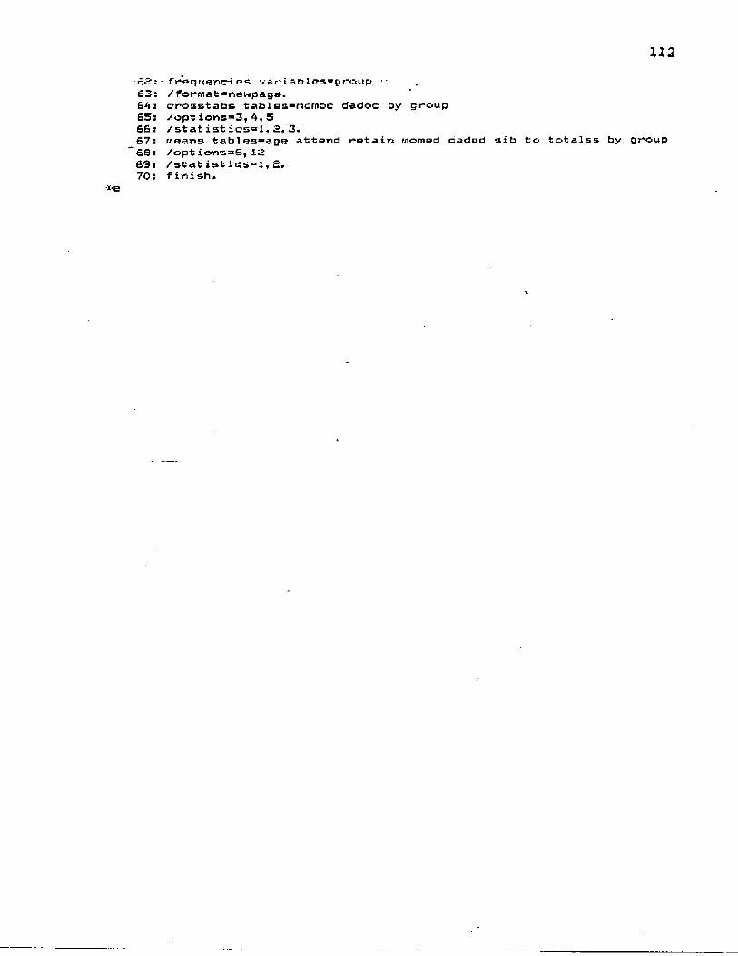
1126.5i - frequencies v e>r~ i sti 1 e3=o r-oup •- £3: / fortnat=newpagB.£4: crosstabs tableS“fiiornoc dadoc by group£5: /opt ioti5»j, A, 566: /statistics=l,£,3.£7 3 means tables™age attend retain monied daded sib to totalss by group £8: /options=S,IS £9 1 /statistics11!, S.70s finish.x-e

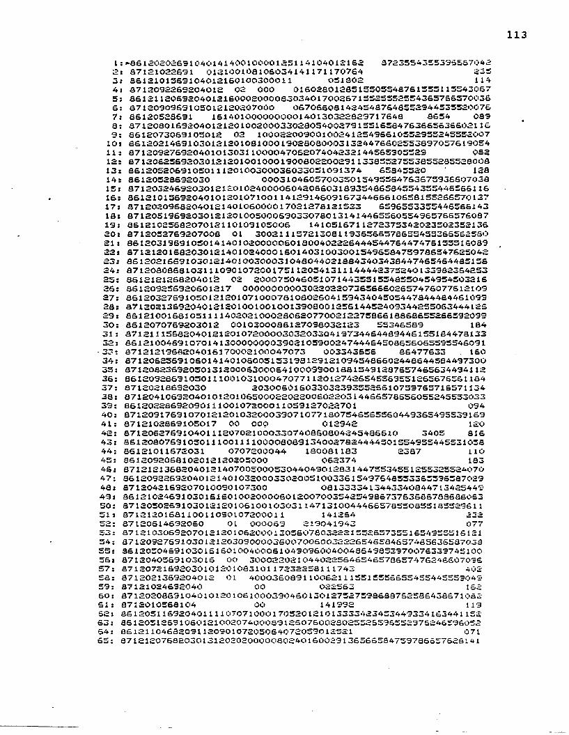
1 j »-aS 120802691040141 400100001851 1 4104012158 37235543553365370482: 87121022631 012100108106034141171170764 £353: 8612101569104012160100300011 051302 1144! 8712092269204012 02 000 01602801265155055487615531155430675: 86121120692040121600020000830340170026713525552534365766570036 6: 8712090969105012120207000 06706608142454876485529445355200767 i 86120528691 161401000000000140130322829717648 8654 0898: 87120801692040121201002000330280540027915516584763665636602116 9: 8612073069103012 02 100022009001002412549661055295524553200710i 86120214691030121201081000190280800031324476602553897057619054 11J 871209276920401013031100004706207404232144565305329 08212: 87120625692030121201001000190080220029113383527553855285528008 13: 8612052069105011120100300036033051091374 65845520 12814: 86120528692030 00031046057003501549356476367593660703815: 87120324692030121201024000060420660318935486584554335446555116 16: 86121015692040101201071001141291460916734466610658155266570137 17: 8712020968204012140106000017021278121533 659655335544656614318: 87120519692030121201005000690330780131414465560554965766576087 19: 8612102568207012110109105006 141051671127237534202350235213620: 8712052769207008 01 300211157213081193656557865545536656256021: 86120319691050141401020000060180040222644454476447475155515089 22: 87121201682030121401024000160140310030015496584759786547625042 23: 861£0216691030121401003000310480440218843403438447465464485156 24: 87120808681031110901072001751120541311144442375240133982364253 25: 8612121268204012 02 200075046051071443551554855045495450321626: 861209256920601217 00000000003022022073656660265747607761210927: 86120327691050121£01071000781080260415943404505447844484461099 28: 87120213692040121201001001001390800125614452409344255063444126 £9: 86121001681051111402021000280620770021227586618868655266592099 30: 8612070769203012 0010300086127098032123 55346589 18431: 87121115682040121201072000030320330419734464489446155184478133 32 j 86121004691070141300000000390210590024744464508655065595546091 33: 8712121968204016170002100047073 003343656 86477633 . 16034: 87120625691060141401060051531981291210945486602448644584497300 35: 87120823692050131200063000641000990018815491287557465634494112 36: 86120928691050111001031000470771120127426545569551255676561184 37: 87120218692030 203006016033032393552661075976571557113438: 87120410692040101201065000220220060220314466578656055245553033 33: 8612022869209011100107200011059127022701 09440: 87120917691070121201032000390710771807546565560449365495539169 41: 8712102869105017 00 OOO 012942 12042: 87120627691040111207021000330740860804245486610 3405 81643: 861208076910501110011 11000080891340027824444501554955445531058 44: 86121011672031 0707200044 180081183 2387 H O45: 8612092068102012120205000 062374 18346: 87121213682040121407005000530440490128314475534SS12S5325S2407O 47: 86120922692040121401032000330200510033615497648553365595587029 46: 8712042169207010090107300 081333341344334084471342544949: 36121024691030161601002000060120070035425498673763586783686063 50: 87120502691030121201061001030311471310044466578S50Q551Q5529611 51: 8712120168110011090107200011 141264 23252: 87120514692060 01 000069 £19041943 07753: 87121030692070121201062000130560780322215525573551654955516121 54: 871£0927691030121203090000360070060032226546584657465636587038 55: 361205046910301£1601004000610490960040043643853370076339745100 56: 8712040363103016 00 300022021044022564654657865747624660703657: 87120721692030101201083101 17232258111743 40258: 8712021369204012 01 400036069110062111531555565545544555304959: 87121024632040 00 022563 16260: 3712020869104010120 1061000390460130127527598688762586438671062 51: 8712010568104 OO 141932 11962: 861£05116920401 111 07071 OOO 1705201210 13333423453449334163441152 63: 86120512691060121002074000831260760028025526596552376846596052 64: 8612110468203112090107205064072059012521 07165: 87121207682030131202020000080240160083136566584759786657688141

i o : o i' X i . l v i - i J. * i 1*' I C ' O 1 U O O / S l O t i 1 1 1 * + ^ 6 ^ ^ 1 / u U y L i i - 1# / i-*

57: 361£0315692030121201002000390531£10715934435537658944484504147 S3: 37120626681041131402001001330001S31310646548673353935206534535 63j 8612042369103012130103300106067042011342 02370: 8712040469106012 03 000006024001013034654762755047613653016371: 3612013069104012 03 00019 041564 14772: 3712081269105011030106302100104036031034 12673: 8612120568206015100003200000000002002651 02174: 86120102692040141200063000131320240024214444505449744324482031 75: 861204096910301211 00094133046031324 13176: 87120505632050 0100100022053018003671549368897008665971605577: 86120517632040111201061000330290210031415484489750665495543020 78: 87121008681060 00 092084 16979: 8712040969103112120207100005008002091724 25580: 87120923631030121201002000060180320031326533792761565467625100 81: 871201065320501010 400092052108082343342552344785526450118782: 3612022369111012 0007600 041151114339344344663422342724633: 86120913592040 120203000050093031002321552763765676555553602734: 87120117691 0700200017061270210144234343213404475340536085: 86120106692030 100000060104051383446449355124489448215386: 86120830692040121201 200 046204061691549556053084466443702387: 87120730631030110801001000920401010616424454497550455064483132 38: 87121121681050120901061000220020472603844445552550855185520407 39: 871201236920901314 000000501471590813435527627971555346607333 50: 86121206632030141601001000030710630032117606510761586247534069 91: 8612042469105012 0108200036127127052114 14692 : 87120427692030121401092000170470470036015487648864797218697062 93: 871201056920301212010010013313504201232375986738659 20594: 861208256920401212010010003210710009168344555525520 16395: 8612012369105012120103107011023034002352 04036: 8712060863106014140206200028 043003032 06297: 87120606692030071201024000000240400421235516610554976246609217 36 :~ 87120526631040121201031000220380631309442354305446144324470133 33: 87120508692050121201002000331521510033834446596446186656570104

100: 871204256920301612010920006910016701295186387058659 047lOl: 87120916691040121201032000081111040523145485527344244664464307 102: 86121219681030121401061000860300100023745526578553665766580069 103: 86120613681040 12 021000470670320316247538688868666658709122104 : 8712032669103012120100107042030032101324 3432237234112383211105: 86120309691030 000420730520418544445544656055035524122106: 861210236310301216 1000720900170036529689744374837053791054107: 87121023631040131302001000330070100030327586578763665676602034 108: 861201116910311212 200031018071022234552 101109: 8712072758108117140000100133 141224 164110: 8712101668206013 0103000050 002861 023111: 37120914532100141502001000220461020715634454501551255204501128 1*2: 87120626681071 1001310471030416844474468342665764490176113: 86120407692050121200072000330722130321633424508 6552 232114: 86120117532040121202002000280430800121815495532332055415543114 113: 8712110757103112120106200017081123I806326566610450065766572223 116: 87120626692060101203091000640661040224936557627761566547651093 117: 86120608631040101001084040811381330321424442402341433962381033 113: 8712032769103012080207110050032153131504 119113: 37120623691060141501071000551731840224224445530 3444 083120: 86120607631 000130680680028326356584658176247612086

.121: 87120626631040 000220370340027126536602 059122 : 86121009632030141601 3000000200290037216557637658176337634071123: 87120924631030121201071000080300481009045435563655475336537331 124: 87120308671051 000110310511412644434512447855134431167125: 86121118632030161700001000420710360040013683705976637213731061 * 26: 87120402631050120801071000500440460123323415544445744534470054 127: 8712030668105112 07 OOOO1203818320068433844584457 500123: 87121206681030121201061000110360840518124434489447044714460131 123: 8612062563204012100109000050 132012551 113130; 87120426631030141301061000670320630127425525564 087121: 86120503631 10120109200 050 031462 U S

115

1 32: 6 1 1 2v6 3061j2v‘w1 4-1 'tvvOt, 10<.ii a00<£‘i 03)50 3 1 'ij'u i;: 6 z i .'6; i i ;■ l iu.133i 37120503691040 000170190530915144464503447044664465135134s 87120703391040131102070000110311522400042353452447033933425506 135: 371307013910901£120102300IS1 032122 052133: 37120919631070121201091000000000601110044437630353765676307393 137: 33120527692030121201061001060090530221 SI4465541552465765557054 133: 37120217631041121201073000721161641603925437633239034334465229 139: 3312070137103112 0106200053 033051942445 34524475 027140: 87121129691050121201030000690£805000240275?S6aS971S65a73£71122 141: 37120307691030151701041001140530900515345506573449344734501143 142: 86120413691040121401001000390340200037427606584760336737634032 143: 3712101163104013 09 OOO 021792 103144: 36121213631050121307094000310431430S1564 5544446643213444155145 » 37121130391030121202070000110440260713145505550554955205539155 146: 36120330691060131301001000530290200035027578705763676007653013 147: 37120521391040161601005000110470430027424476573550465635557109 148: 36120611692 03120109500022039033051893 178149: 33120420391040 01001000220110130029325434516550344824436001150: 37120906691030121201070000190470430027421276536340323854457131 151: 3612030563107112 07 202114091202002602 060152: 871209£669£03012120100£0004700802200344376086aS973176006636144 153: 37120505691030121203073050140501731504323422402554354934472703 154: 36120115691030 01070000000360440322125434437344255324435065155: 37121001692 00 04003016097355276376539 204156: 361208226910401211 3000250190730021023404505448655224494036157: 86120616692060121202020000030340420221335495543656065596566141 158: 37121203631050 0000190340310124724466536551254935523097159: 37120913691040 070000310590391512144454493342055154463160160: 8612013069203012120009100050030073012361444 5520 103161: 3612120368205012 01081000670340320917333404512447444664463134162: 3612041469104012120100100033 031942 101133: 36120509692040121401001001121200340’20935525613 5532 131164: 3612053169104012090107400053054070002722 147

f

APPENDIX BONE-WAY ANALYSIS OF VARIANCE SUMMARY TABLES FOR TWELFTH GRADE DATA

116

117

Page 3£ SPSS/PC* 12/29/87Summaries of APTSS academic aptitude standard scoreBy levels of GROUP group assignment

Value Lahel Mean Std Dev Sum of Sq Cases1 female attender 48.9000 7.1407 1478.7000 302 male attender 50.5000 8. 4217 2340.5000 343 female nonattender 49.2143 5.8141 912.7143 284 male nonattender 4G.7576 6. 8238 1490.0606 33

Within Groups Total 48.8400 7.1709 6221.9743 125

Analysis of Variance

SourceBetveen Groups

LinearityDev. from Linearity

Within Groups

Sum of Squares240.0251105.4438 135.3813

R - -.1277£221. 9749

Eta - . 1S30

D. F.312

R Squared 121

Eta Squared

BeanSquare80. 2750

105. 4438 £7.SSC7

= .016351. 4213

- . 0373

F1.56112.0506 1. 3164

Slg.. 2024. 1547 . 271 D

118

Page 40 SPSS/PCi- 12/29/8-;SumnariffG of READSS reading achievoment expanded standard acBy levels of GROUP group assignment

Value Label Mean Std Dev Sum of Sq Cases1 female attender 560.7586 91.5726 234795. 310 292 male attender 589.5000 87.8874 254898. 500 343 female nonattender 567.5517 61.3855 105509. 172 294 male nonattender 546. 5429 92. 0404 '288026. 686 35

Within Groups Total 566.0866 84.7393 883231. 666 127

Analysis of Variance

SourceBetveen Groups

LinearityDev. Iron Linearity

Within Groups

Sun of Squares

32892. 37888802. 5063

24289* 8724R = -.0969

883231.6685Eta • . 1895

D. F.312

deanSquare

10964.12636602.5063

12144.9362R Squared => .0094123 7180.7453

Eta Squared *■ .0359

F1.52691.1960 1.6913

Sig.. 2109.2759 . 1835

Page 44 SPSS/PC- 12/29/87Summaries ol LANGSS language achievement, expanded standard aBy levels of GROUP group assignment

Value Label Mean Std Dev Sum a£ Sq Cases1 lemale attender 566.0000 75. 1636 158188.000 292 male attender 543.4839 88.9760 237501. 742 313 lemale nonattender 553.3448 80.8576 183062.552 294 male nonattender 500.3824 74.8623 184944.029 34

Within Groups Total 539.2033 80.1100 763696. 323 123

Analysis of Variance

SourceBetween Groups

LinearityDev. frora Linearity

Within Groups

Sum ol Squares

78431.595657804.3312 20627.2S4SR - -.2620

7636S6.3231Eta = .3052

D. F.3

■ 12

MeanSquare

26143.865257804. 3312 10313.6322

R Squared ” . 0686119 6417.6162

Eta Squared ** . 0931

F4.07389.0071 1.6071

Sig.008600332048

120

Page 43 SPSS/PC- 12/29/07Summaries of HATHSS mathematics achievement expanded standarBy levels of GROUP group assignment

Value Label Kean Std Dev Sum of Sq Cases1 fenale attender 559.0000 76.3932 157570.000 282 male attender 548.7879 04.3500 227677.515 333 female nonattender 349.0000 67.3709 108932.000 254 male nonattender 509.7273 79.9126 ,204352. 545 33

Within Groups Total 340.5714 77.9371 698532.061 119

Analysis off Variance

SourceBetveen Groups

LinearityDev. iron Linearity

Within Groups

Sum of Squares

43261.002325323. 5442 9737. 5300

R • -.2185690332. 0606

Eta » . 2467

KeanD. F. Square

3 15087.0274

1 35523.Sa422 4066.7690

R Squared » .0470115 6074.1910

Eta Squared ■* . 0609

F ‘2.48305.8483 . 8016

Sig.. 0643. 0172 .4511

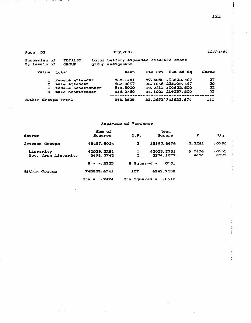
121

Page 52 SPSS/PC-*- 12/29/07Summaries of TQTALSS total battery expanded standard scoreBy levels of GROUP group assignment

Value Label Mean Std Dev Sum of Sq Cases1 .female attender 265.1481 87.4056 198633.407 272 nale attender 562. 8667 88.1045 225109.467 303 female nonattender 548.5000 69.2213 100623.500 224 raale nonattender 515.3750 84.1001 219257.500 32

Within Groups Total 546.8829 83.3652 '743623.874 111

Analysis of Variance

SourceBetveen Groups

linearityDev. from linearity

Within Groups

Sura of Squares

48497. 803442029. 2291 9498.2742

R = -.2303743623.8741

Eta « .2474

D. F. 31

MeanSquare

18165. 867842029.2291 3234.1872

R Squared =■ . 0531107 8949.7558

Eta Squared « . 0612

F

2.3281 6,0476

Slg. . 0788 . 0155. 6790

122

Page 13 SPSS/PC* 12/29/67Summaries of By levels of

RETAIN number of years retainedGROUP group assignment

Value Label Mean Std Dev Sum of Sq Cases1 female attender .0266 . 1690 .9714 352 male attender . 1*163 . 3244 4. 4166 433 female nonattender . 0303 . 1741 .9697 334 male nonattender . 1739 . 3632 6.6067 46

Within Groups Total .0955 .2911 12.9684 157

Analysis of Variance Sun of Mean

Source Squares D. F. Square F Sig.Between Groups . 5965 3 . 1995 2. 3S35 . 0743

Linearity .2733 1 .2733 3.2246 .0/^1Dev. from Linearity . 3251 2 .1626 1.9176 . 1504

R » .1419 R Squared - .0201Within Groups 12. 9664 153 . 0646

Eta ■ . 2100 Eta Squared . 0441

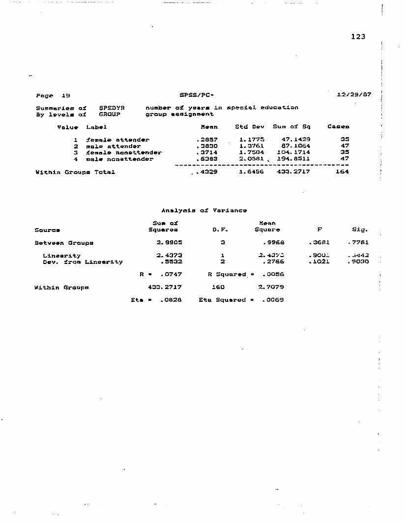
Page 19 s p s s /pci 12/29/37Summaries of By levels of

SPEDYR number of years In special educationGROUP group assignment.

Value Label Mean Std Dev Sum of Sq Cases1 female attender . 2aS7 1.1775 47.1429 352 male attender . 3330 1.3761 37.1064 473 female nanattend»r . 3714 1.7504 104.1714 354 male nonattender . 6333 2.0531 v 194.8511 47

n Groups Total ..4329 1.6456 433.2717 164

Analysis of Variance Sum of Mean

Source Squares D. F. Square F Sig.Between Groups 2. 9905 3 . 9963 . 3631 . 7761

LinearityDev. from Linearity

2.4373 .5532

12

2. 4373 . 2766

. 9001

. 1021. 04-i2 . 9030

R ■ .0747 R Squared = .0056Within Groups 433.2717 160 2. 7079

Eta ■ .0323 Eta Squared . 0069

124

Pago AI SPSS/PC-* 12/29/37Summaries of ATTEND number of schools attendedBy levels of CROUP group assignment

Value Label Mean Std Dev Sum of Sq Cases1 female attender 4.2837 1.6009 87.1429 352 male attender 4.2500 1.2782 70.2500 443 female nonattender 4.3455 1.7694 100.1818 334 male nonattender 4.7556 2.0018 v 176.3111 45

Within Groups Total 4.4630 1.6840 433.38Sa 157

Analysis of VarianceSum of Mean

Source Squares D.F. Square FBetween Groups 7.1715 3 2. 3903 . 8430 *

Linearity 6. 1951 1 6.1951 2.1845 *

Dev. from Linearity .9765 2 * . 4882 . 1722 •ft « .1185 R Squared = .0140

Within Groups 433.3858 153 2.8359Eta * • 1275 Eta Squared « . 0163

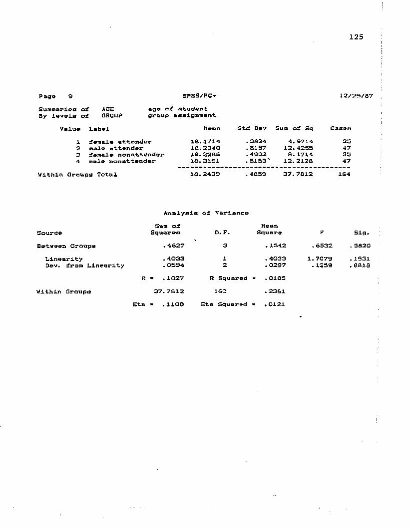
125

Page 9 S P S S / P O 12/29/87Summaries of AGE age a£ student.By levels ol GROUP group assignment

Value Label Mean Std Dev Sum ol Sq Cases1 female attender ia . 1 7 1 4 . 3824 4.9714 352 male attender 1G.2340 . 5197 12.4255 473 ianale nonattender 18.2288 . 4902 8.1714 354 male nonattender 18.3191 .5153' 1 2 . 2 1 2 a 47

Within Groups Total 18.2439 . 4659 37.7812 184

Analysis of Variance Sum ol Hean

Source Squares D.F. Square F Slg.Betveen Groups . 4827 3 . 1S42 . 6532 . 5820

Linearity . 4033 1 . 4033 1.7079 . 1931Dev. from Linearity . 0594 2 . 0297 . 1259 . aaia

R ■ .1027 R Squared - .0105Within Groups 37.7812 180 . 2381

Eta « .1100 Eta Squared - .0121

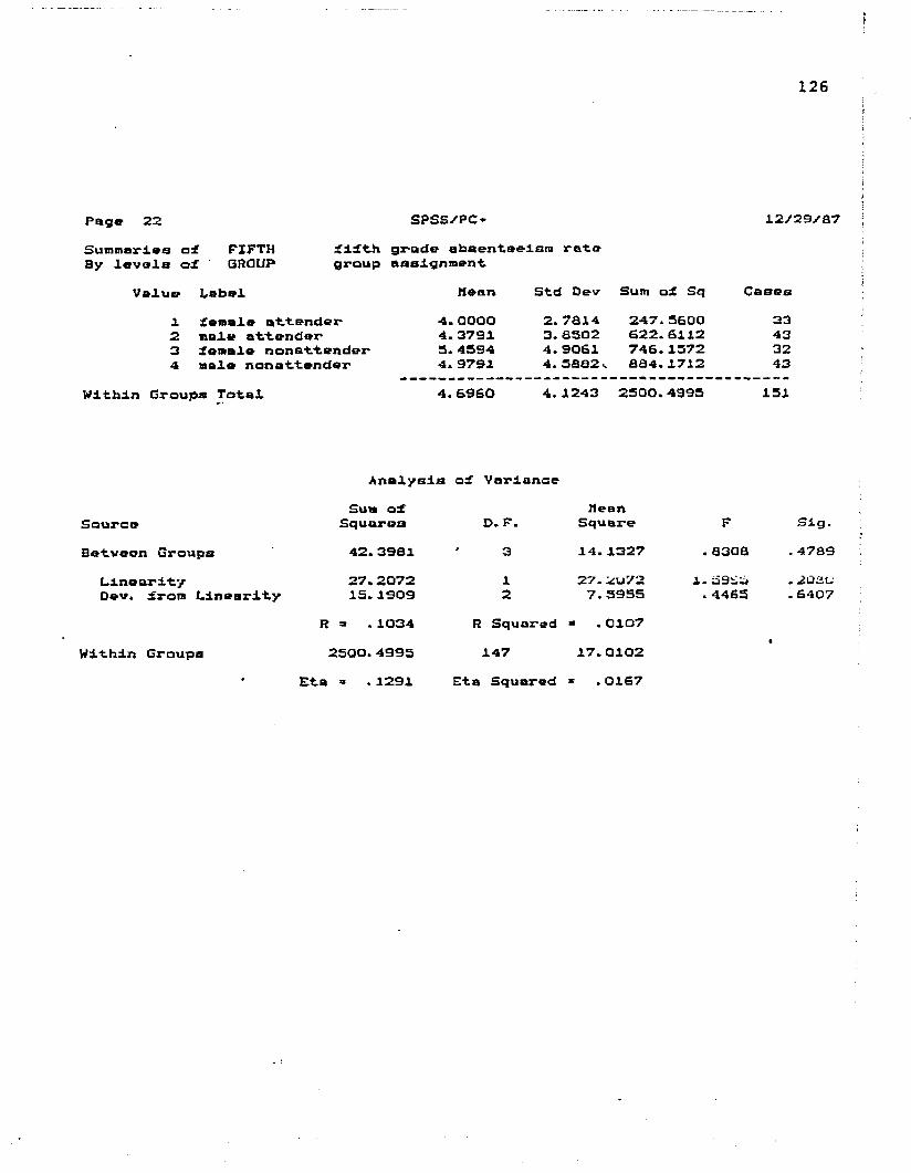
126

Page 22 SPSS/PC- 12/29/37Summaries of FIFTH By levels of ' GROUP

filth grade absenteeism rate group assignment

Value Label Mean Std Dev Sum of Sq Cases1 female attender 4.OOOO 2.7ai4 247* 5600 332 rale attender 4.3791 3.6S02 622*3112 432 female nonattender 3. 4594 4.9031 746.1572 324 male nonattender 4.9791 4.3332v 634.1712 43

Within Groups Total 4. 8930 4. 1243 2500.4995 151

Analysis of Variance Sua of Mean

Source Squares D. F. Square F Slg.Betveen Groups 42. 3981 3 14.1327 . 8308 . 4789

Linearity 27.2072 1 27-2U72 1. . 2Q8LDev. from Linearity 15.1909 2 7.5955 . 4435 . 3407

R = * 1034 R Squared - .0107Within Groups 2500.4995 147 17.0102

t

* Eta * . 1291 Eta Squared - .0167

127

Page 24 SPSS/PC* 12/29/87Summaries of By lovels of

SEVENTH seventh grad» abficnteeiaa rateGROUP group assignment

Value Label Mean Std Dev Sum of Sq Cases1 female attender 3.3313 3. 8485 412.6488 322 male attender 5.4974 4. 3797 728.9097 393 female nonattender 6.9452 5.5089 910.4368 314 male nonattender 3.6488 4, 4046 ' 776.0224 41

Within Groups Total S.8175 4.5106 2828.0177 143

Analysis of Variance

SourceSum of

Squares D.E.Mean

Square F Sig.Betveen Groups 52.1486 3 17.3829 . 8544 . 4665

Linearity 7.4300 1 7.4300 .3632 . 5466Dev. from Linearity 44.7186 2 22.3593 1.0990 . 3361

Within GroupsR - .0506 2828.0177

Eta « .1346

R Squared 139

Eta Squared

> .0026 20.3455

= .0181

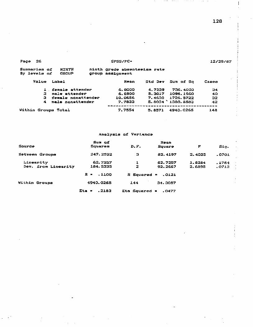
Page 26 SPSS/PC* 12/29/87SunimarlaB of NINTH ninth grade- absenteeism rateBy levels of GROUP group assignment

Value Label Mean Std Dev Sum of Sq Cases1 .. female attender 6 .aooo 4.7239 736.4000 342 male attender 6.6900 5.3017 1096.1960 403 female nonattender 10.0636 7.4630 1726.3722 324 male nonattender 7.7833 5.8034 " 1380.8583 42

Within Groups Total 7.7354 5.8571 4940.0265 148

Analysis of VarianceSum of Mean

Source Squares D. F. Square FBetveen Groups 247.2392 3 82.4197 2.4025

Linearity 62* 7257 1 62.7257 1.8284Dev. from Linearity 184. 3333 2 92.2667 2.6895

R - .1100 R Squared » .0121Within Groups 4940. 0265 144 34.3057

Eta “ . 2183 Eta Squared ■ .0477

Sig.070117e40710

Page 54 SPSS/PCi 12/29/87Sunnarlea ol By levels ol

TWELVE tvellth grade aba«nteeiaii) roteGROUP group assignment

Value Label Mean Std Dev Sum ol Sq Cases1 lemale attender 6.6057 3.5832 436.5389 352 male attender 9.6553 iO.3191 4898.2962 473 lemale nonattender 16.3229 10.aioo 3973.0817 354 male nonattender 22.6170 16.3444 12288.4464 47

n Groups Total 14. 7543 i i .s ia o 21596.3631 164

Analysis ol VarianceSum ol Mean

Source Squares D. F. Square F Sig.Betveen Groups 7209.5039 3 2403.1680 17.8042 O. O

Linearity 6925. 8504 1 6925.8504 51.3112 . OOOODev. from Linearity 283.6535 2 141.8267 1.0507 . 3521

R * .4903 R Squared . 2404Within Groups 21596.3631 160 134.9773

Eta * . 5003 Eta Squared a .2503

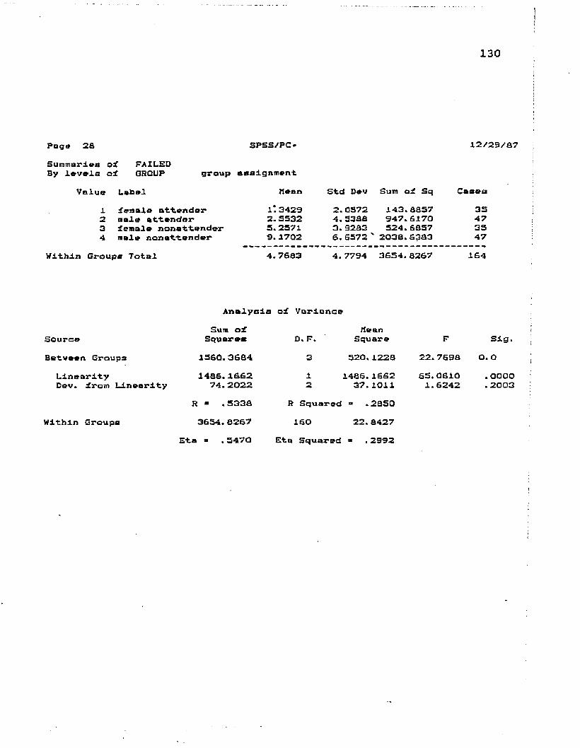
130

Page 26 SPSS/PC* 12/29/37Summaries of By levols of

FAILEDGROUP group assignment

Value Label Mean Std Dev Sum of Sq Cases1 female attender 1* 3429 2.0572 143.6657 352 male attender 2.5532 4.53d6 947.6170 473 female nonattender 5.2371 3.9263 524.6857 354 male nonattender 9. 1702 6.6372 ' 2038.6383 47

Within Groups Total 4.7663 4.7794 3654.8267 164

Analysis of Variance

SourceBetveen Groups

LinearityDev. from Linearity

Within Groups

Sum of Squares

1260.26641466.1662

74.2022R - .53363654. 8267

Eta ■ . 3470

D. F.312

MeanSquare

520.1228I486.1662

27.1011R Squared » .2630160 22.6427

Eta Squared 3 . 2992

F22.769a65.0610 1.6242

Sig. O. 0

. oooo

. 2003

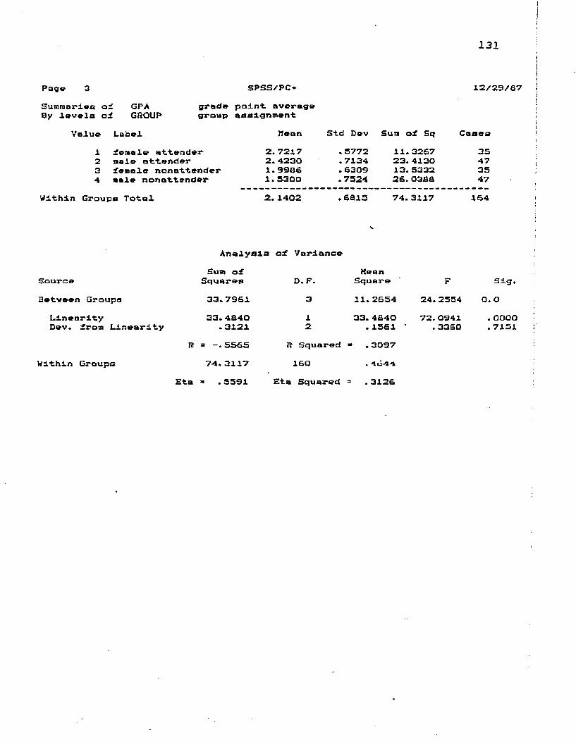
131

Page 3 SPSS/PC» 12/29/87Summaries of GPA grad* point averageBy levels al GROUP group assignment

Value Label Mean Std Dev Sun ol Sq Cases1 lemale attender 2.7217 .5772 11* 3267 352 sale attender 2. 4230 .7134 23.4130 473 lemale nonattender 1.9986 . 6309 13.5332 354 aale nonattender 1.5300 .7324 26.0368 47

Within Groups Total 2. 1402 .6815 74.3117 164

Analysis of Variance Sum ol Kean

Source Squares D. F. Square F Sig.Betveen Groups 33.7961 3 11.2654 24. 2554 Q. O

Linearity 33.4840 1 33.4840 72. 0941 . ooooDev. Iron Linearity .3121 2 .1561 * . 3360 . 7151

R = 5565 R Squared » .3097Within Groups 74.3117 160 . 4u44

Eta - .5591 Eta Squared . 3126

132

Page & SPSS/PC* 12/29/37Summaries al HOMED mother's educational levelBy levels ol GROUP group assignment

Value Label Mean Std Dev Sum al Sq Cases1 lemale attender 12.4373 1. 3698 59.8750 322 male attender 12.3122 1. 6751 112.2439 413 lemale nonattender 11.5517 i. ao45v 91.1724 294 male nonattender 12.4615 1.4113 ' 75.6923 39

Within Groups Total 12. 2637 1. 5730 336.9836 141

Analysis al Variance Sus al Mean

Source Squares D. F. Square F Sig.Betveen Groups 19.6669 3 6.5363 2.6497 . 0514

LinearityDev. Irani Linearity

- 6510 18.8179

12

. S510 9.4089

. 3439 3.6026

. 5585

. 0247R - -.0467 R Squared » .0024

Within Groups 338.9836 137 2. 4743Eta - .2342 Eta Squared a .0548

Page 15 S P S S / P O 12/29/87Summaries of OADED father's educational' levelBy levels of GROUP group assignment

Value Label Mean Std Dev Sum of Sq Cases1 female attender 12.5667 1.8860 103.3667 302 male attender 12.3611 2.0723 150.3056 363 female nonattender 12.6000 1.8257 80.0000 254 male nonattender 12.0588 1.9991' 131.8824 34

Within Groups Total 12.3760 1.9615 465. 5546 125

Analysis of Variance

SourceBetveen Groups

LinearityDev. from Linearity

Within Groups

Sue of Squares

5.77342.9537 2.9197

R » -.0792465.5546

Eta » . 1107

D.F.312

R Squared 121

Eta Squared

MeanSquare1.92452.9537 1.4099

> .0063 3.8476

> .0122

F. 5002. 7677 . 3664

Sig.682938276940

134

Page 1? SPSS/PC* 12/:Summaries ol SIB number ol siblings residing in homeBy levels ol GROUP group assignment

Value Label Mean Std Dev Sum ol Sq Cases-1 lemale attender 1.8235 1.4662 70.9412 342 male attender 1.5227 1.2848 70.9773 443 lemale nonattender 1.£970 1.3343 56.9697 334 male nonattender 1.3902 1.3206 ' 69.7561 41

Within Groups Total 1.5921 1.3473 268.6442 152

Analysis ol Variance Sum al Mean

Source Squares D.F. Square F Sig.Betveen Groups 4.0663 3 1.3554 .7467 . 5259

LinearityDev. Irani Linearity

2.3390 1.7273

12

2.3390.8637

1.2886 . 4758

. 2581

. 6223R » -.0926 R Squared 3 .0086

Within Groups 268.6442 14a 1.8152Eta > .1221 Eta Squared = .0149

APPENDIX CCHI-SQUARE PROCEDURE FOR PARENTSf OCCUPATIONAL LEVELON TWELFTH GRADE DATA

135

136

Page 4C r o a a t a b u l a t i o n : H O K Q C

B y G R O U P

SPSS/PC*■

nothar's occupational levelgroup assignment

Count IRow Pet tfenale a Imale attIfemale nI male non I

GROUP-> Col Pot Ittender 1«nder I onattendt attenderIITot Pet 1 1 1 2 1 3 1 4MOMOC --------

O 1 6 1 2 1 4 J 4professional, te I 37. 5 J 12. 5 1 25.0 J 25. 0

1 17. 6 1 4.9 1 14. 3 1 IO. 51 4. 3 1 1. 4 1 2 . a 1 2 . a

1 r 23 1 30 t 1 7 1 2 1

homemaker 1 23. 3 1 33. O 1 18.7 1 23. 1

1 67. 6 1 73. 2 J 60. 7 1 55. 3t 16. 3 t 21.3 t 1 2 . 1 1 14. 9

2 1 3 1 5 1 4 1 7clerical & sales 1 13. a 1 26. 3 1 2 1 . 1 1 3 6 . a

t s . a ) 12.2 J 14. 3 1 l a . 41 2. 1 1 3. 5 1 2 . a 1 5. O

3 1 1 1 2 1 l t 2

service 1 16.7 t 33.3 1 16. 7 1 33. 31 2. 9 1 4. 9 t 3. 6 J 5. 31 . 7 1 1. 4 1 . 7 t 1. 4

7 » « 1 1 I 2 i 4

benchwork 1 12. 3 1 12.3 1 25. 0 1 5 0 . 0

1 2. 9 1 2.4 1 7 . 1 1 IO. 5J . 7 J . 7 1 1.4 I 2 . a

9 1 1 1 1 J

miscellaneous 1 i lOO.O 1 1

t 1 2.4 t >

1 t . 7 1 1Column 34 41 2a 38Total 2 4 . 1 29. 1 19. 9 27. O

Chi-Square D. F. S i g n i f i c a n c e Min E. F.

i O . 9S347 1 5 7559 . 1 9 9

B o v

TotalIS

11. 3

9 1

6 4 . 5

19 13. 5

64 . 3

45. 7

1 . 7

141 lOO. 0

Cells vith I

IQ OF 24 <Statistic Value Significance

Cramer's VContingency Coefficient

.16092

.26849

12/29/87

. F. < 5

75. OK)

Humber of Missing Observations 3 23

Page 5Croaatabulationt DADOC

fly GROUP

SPSS/PC*father's occupational levelgroup aaalgninent

Page

CountRow Pet 1female a 1 sale attlfemale n 1 male nonJ

GROUP-> Col Pet 1ttender lender 1 onattend1attender1 RowTot Pot 1 i 1 2 1 3 1 4 1 Total

DADOC --------0 1 9 1 11 1 9 1 a 1 37

professional, te t 24. 3 1 29. 7 1 24.3 1 21. 6 1 2a. 51 30.0 1 29. 7 1 33.3 1 22. 2 11 6.9 1 0.5 1 6.9 1 6. 2 1+

2 1 2 1 2 1 5 1 3 '1 12clerical & sales 1 16.7 1 16.7 1 41.7 1 25.0 1 9. 2

1 6.7 1 5. 4 1 ia. 5 1 a. 3 Jt 1.5 1 1. 5 I 3. a 1 2. 3 r♦ ■

3 1 5 J 3 1 1 2 i IOservice J 50. 0 1 30. O 1 1 20. 0 i 7. 7

I 16.7 1 a. 1 1 1 5. 6 i1 3. a 1 2.3 1 1 1.5 i+ •

4 1 I 1 1 1 i 1agricult. H a h , r 1 1 1 lOO. o i .8

i 1 1 1 2. a ii 1 1 1 .a i

S i i jI 1 l I 1processing i 1 1 1 100. 0 i . a

i 1 1 1 2. a ii 1 11 I . a i

6 i 6 1 6 11 2 1 5 i 19machine trades ( 31.6 1 31. 6 11 10. s 1 26. 3 I 14. 6

i 20. 0 1 16. 2 1 7.4 t 13. 9 ii 4. 6 1 4. 6 1 1.5 1 3. a i

7 i 2 1 a 1 6 1 11 i 27benchwork i 7. 4 1 29. 6 1 22. 2 1 40. 7 i 20. a

i 6. 7 1 21. 6 1 22. 2 1 30. 6 ii 1. 5 1 6.2 1 4. 6 1 a. 5 i

a i I 2 1 2 1 2 i 6structural t 1 33. 3 1 33.3 1 33. 3 i 4. 6

i 1 5. 4 1 7. 4 1 5. 6 ii I 1.5 1 1. 5 1 1. 5 i

9 i 5 I 3 1 2 t 3 i 13miscellaneous i 33. 5 1 23. I 1 15. 4 1 23. 1 i 10. O

i 16. 7 1 a. l i 7. 4 1 a. 3 ii 3. a I 2. 3 1 1. 5 1 2. 3 i

IO♦ “i 1 1 1 1 1 i 2

self-employed i 1 50. 0 1 50. O 1 i 1. 5i 1 2. 7 t 3. 7 1 ii 1 . a i . a 1 i

Column 30 37 27 36 130(Continued) Total 23. 1 2a. 5 20. a 27. 7 1O0. 0

137

12/29/87

1 of 2

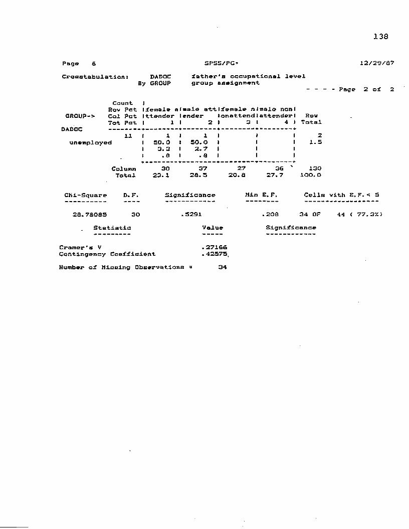
138

Page S Crosatsbulstiom

SPSS/PC-DADOC father's occupational level

By GROUP group assignment- - Page

GROUP->DADOC

Count IRov Pet I female a I male attIfemale nI male non I Col Pet Ittender lender lonattendtattenderI Tot Pot I 1 1 2 1 3 1 4 1

11 Iunemployed

ColumnTotal

150. 03. 3

.a

i50.02.7

. a

i

30 23. 1

37 28. 5

27 20. 8 36

27. 7

RovTotal

21.5

130 lOO. 0

Chi-Square D.F. Significance Min E. F. Cells vith E.

28.78085 30Statistic

. 5291Value

.208 34 OFSignificance

44 (

Cramer's VContingency Coefficient

.27166

.42575Humber of Missing Observations = 34

12/29/87

2 of 2

F. < 5

77.3 f )

APPENDIX DPEARSON PRODUCT MOMENT CORRELATION COEFFICIENTS ON TWELFTH GRADE DATA

139

140

Page 2 Correlations:

AGE

a t t e n d

RETAIN

HOMED

DADED

SIB

SPEDYR

FIFTH

SEVENTH

NINTH

TWELVE

FAILED

GPA

APTSS

READSS

HOMED DADEDAGEi.oaoo( 78)pa .

09 87 t 78) P= .400

. 6423 ( 78)P= . OOO-.0617 ( 78)P=* . 592-.0706

.'( 7 S ) P- .539

. 0559 ( 78)pa . 627

0859 ( 78)P» .455

.0213 C 78) P» .853

0841< 78) P» .464

. 0664< 78) P= .563

. 2071< 78) P*. . 069

. 3574< 78) Pa .OOl

2980 ( 78)P» .0Q8

. 0576 ( 78)Pa .616

. 0104 ( 78)pa .928

ATTEND-.0967

{ 78)pa .4001.OOOO ( 78)P» .-.0690

t 78) P - .548

.0380 ( 78)

P a .741-.0296

t 78) P - .797

-.2110 ( 7a)

p a .064. 0246

t 78) p a .831-.0246 t 78)

p a .831.2063

< 78) P » .070

.1928< 78)

P - .091.0793

< 78) p a .490. 1120

t 78) p a .329-.2165

t 78) P a .057

. 0067 t 78)

p a .954-.0539

( 78)P» .640

SPSS/PC*RETAIN.6423

( 78)P» .OOO-.0690 t 78) P* .5481.0000 ( 78)P* .-.0739< 7a) pa .520-.0544

( 78)pa .636

.0230 t 78) P« ,842-.0521

t 78) pa .651

.2796 ( 78)Pa ,013

.1205 ( 78 >P- .293

.2841 { 78)pa .012

. 2363< 78) pa .037

. 3812 ( 78)P= .001-.3110

( 78)Pa .006

. 1108 ( 78)pa .234

. 0387 ( 78)pa .737

-.0617 ( 78)P= .592

. 0380 t 78)

P a .741-.0739

t 78) Pa .520 v1.OOOO ( 78)P» .

. 6011 ( 78)P» .OOO-.0837

( 78)P» .466-.0086 ( 78)Pa .940-. 0488

( 78)Pa .672-.0338 ( 78)

P a .769-.0772 ( 78)

P a .502-.0596 ( 78)p= .604-. 1121 ( 78)

P a .329. 2180

( 7S) pa .055

. 2029 ( 78)

p a .075. 2076

( 78)pa .068

-.0706< 78) P« .539-.0296

t 78) P» .797-.0544

( 78)Pa .636

.6011< 78)

p o . 0001.0000

< 78) P a .

0383< 78)

P a .7390472

( 78)P= .681

1081 ( 78)

p a .346-.1264 ( 78)

• Pa .270-.2139 { 78)P= .060-.1678 ( 78)

P a .142-.2737

( 78)P a .015

. 3558 ( 78)

P a .OOl. 4603

( 78)P a ,000

. 4089< 78) P= .OOO

1/1/88SIB.0559

( 78)P a .627-.2110

t 78)P a .064

.0230 ( 78)

P = . 842-.0837 ( 78)pa .466-,0383 ( 78)

P a .7391.OOOO ( 78)

P a .

. 0775 < 76)

p a . 500-. 0405

( 78)P a .725

.0859 ( 78)

P a .454. 0664

( 78)P= .564-.1122

( 78)Pa . 328-.1216

( 78)P = .289

. 1371 ( 78)pa .231-. 0609

t 78)P= .596-.0422

( 78)pa .714

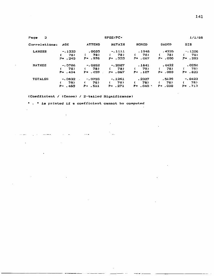
141

Page 3 SPSS/PC* 1/1/88Correlations: AGS ATTEND RETAIN HOMED DADED SIS

LAHGSS 1333 . 0035 1111 . 1948 . 4335 1206( 78) ( 78) ( 78) ( 78) ( 78) ( 78)P= .245 P=* .976 Pa .333 Pa .087 Pa .OOO P= .293

MATHSS 0786 0852 -.2087 . 1841 . 4432 . 0258( 78) < 78) < 78) ( 78) ( 78) ( 78)P= .434 P = .459 . P= .067 Pa .107 Pa .000 P= .823

TQTALSS -.0832 -.0755 1261 . 2327 .5139 -. 0423< 78) ( 78) ( 78) ( 78) ( 78) ( 78)P= .469 P = .511 P= .271 P “ . 040 '■ Pa .000 Pa .713

(Coefficient / (Cases) / 2 --tailed Significance)■ . ■ is printed if a coefficient cannot be computed

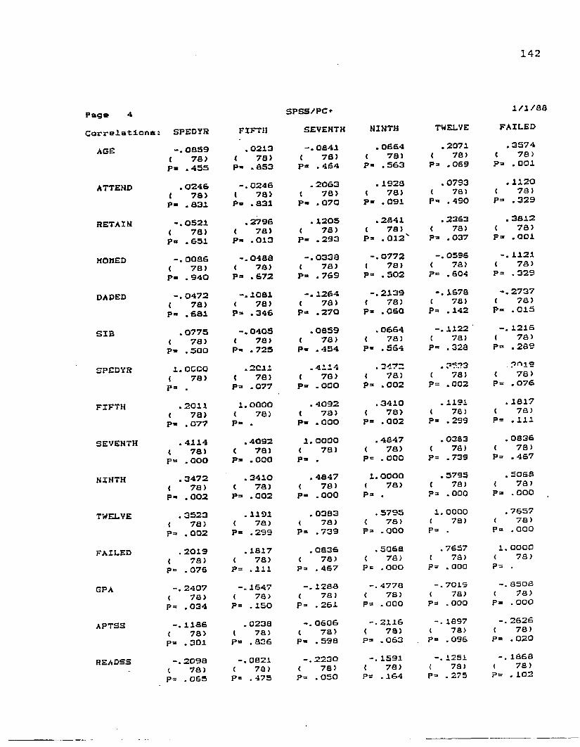
142

Correlatlona: SPEDYRPage 4

ACE

ATTEND

r e t a i n

h o m e d

DADED

SIB

SPEDYR

FIFTH

SEVENTH

NINTH

TWELVE

FAILED

GPA

APTSS

READSS

-.0859 ( 78)P» .435

.0246 ( 78)P- .831-.0521

( 78)P» .651

0086 ( 78)P- .940

0472 ( 78)P» .681

.0775 ( 78)P* .5001.OCOO ( 78)P= ..2011

( 78)pa .077

. 4114 < 78)pa .OOO

.3472 ( 78)P« .002

. 3523 ( 78)pa .002

. 2019 ( 78)pa .076

2407 t 7 8 )

Pa .034-.1186 ( 78)pa .301-.2098

( 78)Pa .065

FIFTH. 0213

< 78) P- .853-.0246 ( 78)Pa .831

. 2796< 78) Pa .013-.0488

< 78) P= .672-.1081

( 78)Pa .346

0405 ( 78)Pa .725

.2011 ( 78)Pa .0771.0000 ( 78)Pa .

.4092 ( 78)pa .000

. 3410 t 78} Pa .002

. 1191 ( 7a) P= .299

. 1817< 78) P= .Ill

1647 ( 78)P= .150

. 0238 ( 78)P» .836

0821 C 78) P= .475

SPSS/PC*SEVENTH-.0841 ( 78)pa ,464

. 2063< 78) pa .070

. 1205 ( 78)pa .293-.0338

< 78) P- .769

1264 ( 78)P« .270

.0859 ( 78)pa .454

.4114 t 78) Pa .OOO

. 4092 t 78) Pa .0001.OOOO ( 78)Pa .

. 4847 ( 78)P« .000

. 0383 ( 78)P= .739

, 0836 ( 78)Pa .467-.1288< 78) P= .261

0606 ( 78)Pa .598

2230 ( 78)pa .050

NINTH. 0664

< 78) pa .563

. 1928< 78) P- .091

.2841 ( 78)Pa .012''-.0772

( 78)P“ .502-.2139

t 78)p a .060

. 0664 { 78)

P a .564. 3472

( 78)p a .002

.3410 t 78)

P = .002.4847

( 78)P = .OOO1.0000 t 78) Pa .

.5795 ( 78)pa .OOO

. 5068 ( 78)Pa .OOO

4778 t 78) Pa .000-.2116

< 78) pa .063

1591 ( 78)Pa .164

TWELVE.2071

( 78)Pa .069

.0793 ( 78)Pa .490

.2363 ( 78)Pa .037

0596 ( 78)P= ,604-.1673 ( 78)P= .142

-.1122 ( 78)Pa .328. P533

{ 78)P= .002

. 1191 < 78)pa .299

.0383 ( 78)P= .739

.5795( 78)Pa .0001. 0000 C 78) P = .

. 7657 t 7a) p» .000

7019 t 78) Pa .000

1897 « 78)pa .096-.1251

( 78)Pa .275

i / i / a a

FAILED. 3574

t 78) p a .OOl

. 1120 ( 78)

P a .329. 3612

< 78)P a .OOl-.1121

( 78)P a .329-.2737 ( 78)

P a .015-.1216 ( 78)

P a .289?nl9

( 78)P = .076

. 1817< 78)

P = .111. 0836

t 78) p a .467

. 5068< 78)

P a .OOO. 7657

( 78)P= .OOO1.OOOO ( 78)P= .

8508 ( 78)P= .OO0

2626 ( 78)

P a .0201868

< 78)p a .102

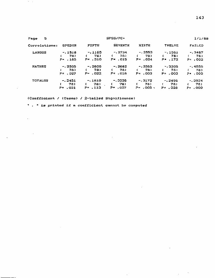
143

Page S Correlations:

LANGSS

MATHSS

TOTALSS

(Coef ficient

SPSS/PC*SPEDYR FIFTH SEVENT]

1518 -. 1165 -.2734< 78) ( 78) ( 78)P= .185 F*» .310 P = .015

2505 -.2600 -.2682< 78) ( 78) ( 78)Pa , 027 P= .022 P= .018-. 2451 1810 -.3038

( 78) ( 78) ( 78)P = .031 P= .113 P- .007

1/1788NINTH TWELVE FAILED

2553 -. 1561 -. 3487< 78) ( 78) ( 78)P=> .024 P= .172 P= .002-.3363 3305 -.4555( 78) < 78) ( 78)Pa .003 pa .003 pa ,000

-.3172 -.2496 -. 3924< 78) { 78) ( 78)P= .005 v Pa .028 pa .OOO

/ (Cases) / 2-tailed Significance)is printed if a coefficient cannot be computed

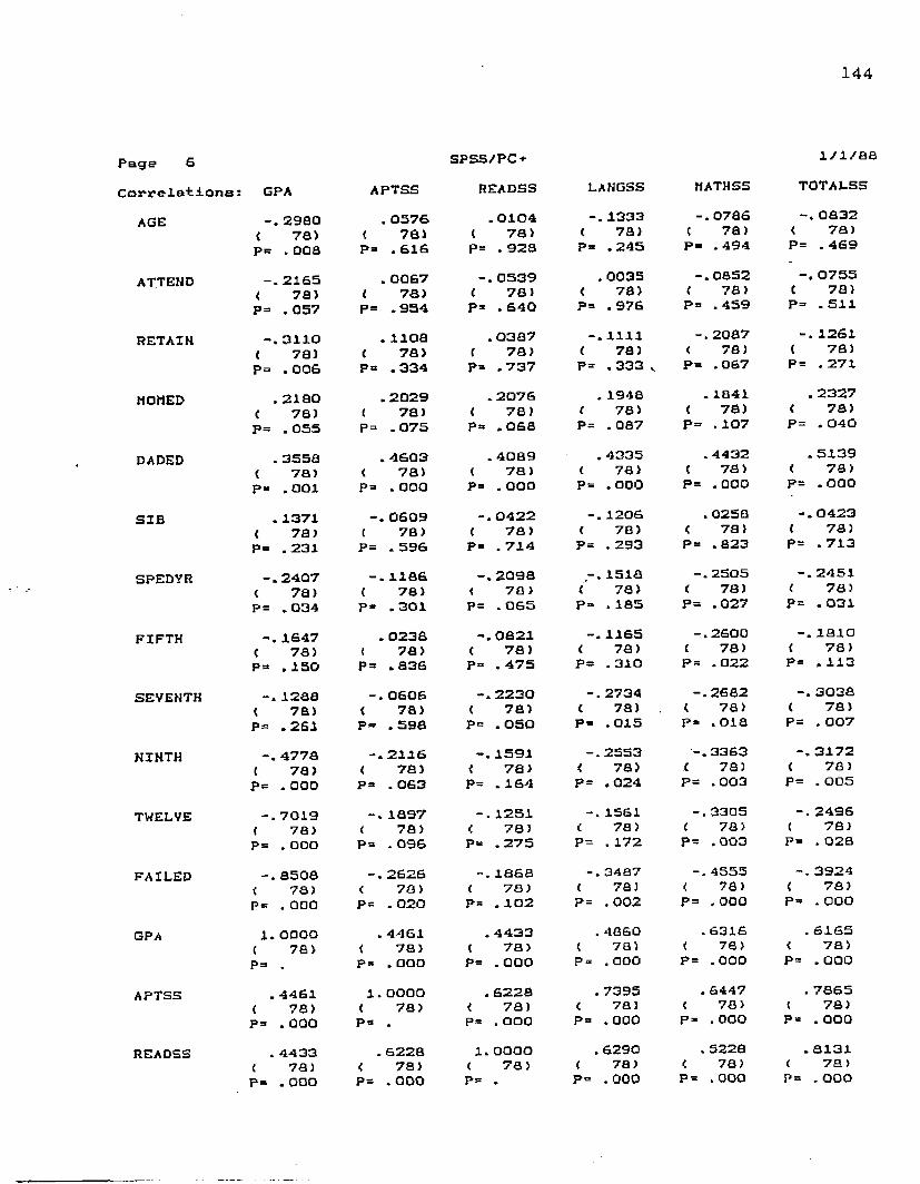
144

Page 6 Correlations:

AGE

ATTEND

RETAIN

HOMED

DADED

SIB

SPEDYR

FIFTH

SEVENTH

NINTH

TWELVE

FAILED

GPA

APTSS

READSS

GPA2980

( 78)P = .008-. 2165 < 78)P= .057

3110 t 78) P= .006

. 2180 ( 78)P=j . 055

. 3558 ( 78)P= .OOl

. 1371 ( 78)P= .231-.2407

£ 7a >P= .034

1647 ( 78)P= .150

1288 £ 78)P= .261~.4778 ( 78)P= .000

7019 ( 78)P= .OOO-.8508

( 78)P= .0001. OOOO

t 78) P= .

. 4461 £ 78)pa .000

. 4433 ( 78)Pa .OOO

APTSS. 0576

( 78)P= .616

. 0067 f 78) P= .954

. 1108 ( 78)P** . 334

. 2029 ( 78)Pa .075

. 4603 £ 78)P= .OOO

0609 £ 78)P= .596-.1186 ( 78)P= .301

. 023S ( 78)P= .836-.0606

t 7a> P= .598-.2116

< 78)P = .063-.1897 ( 78)P» .096-.2626

( 78)P= .020

. 4461 ( 78)pa .OOO1.OOOO

( 78)P« .

. 6228 ( 78)Pa .OOO

SPSS/PC+READSS. 0104

( 78)P= .92S-. 0539 £ 78)P* .640

.0387 t 78) pa .737

.2076 ( 78)P« .068

. 4089 ( 78)Pa .OOO

0422 ( 78)P= .714-.2098< 78) pa .065-. 0821 C 78) P= .475-.2230

( 78)P= .050

1591 { 78)P= .164

1251 ( 78)P= .275

1868 ( 78)P= .102

. 4433 £ 78)Pa .OOO

. 6228< 78) P= .OOO1.OOOO ( 78)P- .

LANGSS-.1333

( 78)p a .245

. 0035 £ 78)P= .976-.1111

( 78)P= .333 „

. 1948 t 78) P= .087

. 4335 ( 78)P= .OOO-.1206

( 78)P= .293-. 1518

£ 78)P= .185-.1165

( 78)P= .310-.2734

( 7 S )Pa .015-.2553

£ 78)P= .024-.1561

( 78)P= .172-.3487

< 78)P= .002

. 4860 { 78)P= .OOO

. 7395 ( 78)P= .000

. 6290 ( 78)P= .000

MATHSS-.0786

( 78)Pa .494-. 08S2

< 78) P= .459-.2087

( 78)P= .067

. 1841 £ 78)P= .107

. 4432 C 78) P= .OOO

. 0258 ( 78)P= .823-.2505

£ 78)P= .027-.2600

( 78)p a . 0 2 2

-.2682 £ 78)P- .018-.3363

< 78) P= .003-.3305

£ 78)P= .003-.4555

( 78)P= .OOO

. 6316 ( 78)P= .000

. 6447 ( 78)P= .OOO

. 5228 ( 78)P= .OOO

1/1/88TOTALSS-. 0832

< 78)P = .469

0755 t 78)

P = .511-. 1261

( 78)P= .271

. 2327 £ 78)

P = .040. 5139

( 78)P = .OOO

0423 ( 78)

P = .713-.2451

£ 78)P= .031-. 1810

{ 78)P = .113-. 3038

( 78)P = .007

3172< 78)

P = .005-.2496 ( 78)

P a .0283924

£ 78)P a . OOO

. 6165< 78)

p a .OOO. 7865

( 78)P = .OOO

. 8131 ( 78)P= .OOO

145

Page SPSS/PC* 1 / 1/88Correlations! GPA APTSS READSS LANGSS MATHSS TOTALSS

LANGSS . 4860 . 7395 . 6290 1.0000 . 6499 . 8727( 78) ( 78) t 78) ( 78) ( 78) C 78)P» .OOO P “ .000 P = .000 P» . P- .OOO P» .OOO

MATHSS . 8316 .6447 . 5238 . 6499 1.0000 . 8649( 78) ( 78) ( 78) t 78) ( 78) ( 78)P* .OOO P- .OOO P- .OOO P “ .OOO P» . P= .OOO

* TOTALSS .6165 .7865 . 8131 . 8727 . 8649 1.OOOO( 78 J ( 78) ( 78) ( 78) ( 78) ( 78)P« .OOO P» .OOO P= .OOO P=* .000 v P» .OOO P= .

< Coefficient / (Cases) / 2-tailed SignificanceJ■ . ■ la printed if a coefficient cannot be computed

APPENDIX EMULTIPLE REGRESSION ANALYSIS AND PLOTS ON TWELFTH GRADE DATA

146

147

Pag* 16 SPSS/PC- 1/1/68• M U L T I P L E R E G R E S S I O N . . . .

Equation Number 1 Dependent Variable.. TWELVE twelfth grade absenteeism Beginning Block Number 15. Methods Enter SEVENTH

Variable!s) Entered on Step Number15.. SEVENTH seventh grade absenteeism rate

Multiple R .85071R Square .72370Adjusted R Square .65686Standard Error 7.9458SAnalysis of VarianceRegressionResidual

DF Sum of SquaresIS 102S3.1229662 3914.46422

F a 10.82640 Signif F . OOOO

Mean Square 683.54153 63.13652

Variables in the EquationVariable B SE a Beta T Sig TFAILED 1.34172 .•21279 .60873 6. 305 . OOOONINTH 1.06174 .28444 .36348 3. 733 .0004SPEDYR 3.09086 1.18767 .20691 2. 602 . 0116MATHSS -7.93354E-Q3 .01923 -.04520 -. 413 . 6813RETAIN -2.59900 S. 65125 -.04723 -.460 . 6472AGE .59403 3.09073 .01833 . 192 . 8482APTSS -.03135 .23830 -.01663 -. 132 . 8958DADED .17094 .67600 .02457 . 253 . 8012LANGSS .02807 .01997 .16867 1.405 . 1649READSS -6.68S71E-03 .01402 -. 04470 -.477 .6351FIFTH 19857 .27981 05670 -.710 . 4806SIB -. 51540 .70773 -.05250 -.728 . 4692ATTEHD 39077 .68830 -.04172 -. 568 . 5723MOHED -.02896 .79764 -3.OQSE-03 -.036 . 9712SEVENTH -.62390 .29004 -.20429 -2.151 . 0354< Constant) -IQ. 18726 57.18686 -. 178 . 8592

End Block Number 15 All requested ■ variables entered.

148

Page 17 SPSS/PC* 1/1/30. . . . M U L T I P L E R E G R E S S I O N * . • •

Equation Number 1 Dependent Variable. . TWELVE tvelith grade absenteeism

Residuals Statistics:Min Max Mean Std Dev N

• PRED -1.7317 57.asai 14.6126 11.5394 76•ZPRED -1. 4164 3.7476 . OOOO 1.OOOO 73•SEPRED 1.7457 6.0639 3. 4764 . 9269 76•ADJPRED -3.0041 53.3632 14.3652 11.3060 » 76•RESID -12.7004 26.6652 OOOO 7.1300 76•ZRESID -1. 5934 3.3539 OOOO . 6973 76•SRESID -1.373a 3.6754 .0124 1.0406 76•DRESID -IS.6299 31.9647 .2476 9.8197 78*SDRESID -1.9136 4.1223 .0209 1.0751 76•MAHAL 2.7294 44.1547 14.6077 8.6639 76•COOK D . OOOO . 524S . Q274 .0696 76•LEVER . 0354 . 5734 . 1923 . 1125 76Total Cases « 164

Outliers - MahalanQbia' DistanceCase ■# AGE -MAHAL

153 16. OO 44.1546934 16. OO 43.2608324 19.00 33.6082529 19. OO 31.7616469 16.00 29. 99426aa 19. OO 26.5066366 19. OO 27.94072

117 ia . oo 27.77429115 20. OO 27.46943150 IS. OO 26.77267

149

Page 18 SPSS/PC-*- i/i/ea

Histogram - Studentized ResidualCases, . :HExp N (• = 1

1 . 06 □ ut *0 . 12 3. 000 . 30 2. 672 . 70 2. 33 I *3 1. 42 2.00 * * *0 2. 61 1.67 .4 4. 28 1. 33 • ** X5 6. 29 1. OO ♦ ♦ * w #4 8. 28 .67 «**•8 9. 77 . 33* 10. 3 0. O• 9. 77 33a 8.28 -.676 6. 29 -1. 00 • • ♦ ♦ ♦3 4.28 -1. 334 2. 61 -1. 672 1. 42 -2. 00 : *0 . 70 -2. 33 #0 .30 -2- 670 . 12 -3. OO0 .06 □ut

Normal Curve)

Normal Probability tP-P) Plot Standardized Residual

1.0 * ---------------

. 25 . 75- - - Expected 1. 0

150

Page 19 SPSS / P O

Standardized Scatterplot Across - »PRED DownOut ♦3 +

-SRESID

-1

-2

. » i

—3 + Out ■*■--

-3

Symbols: Max N

3 Out

1.0 2. 0 5. 0

i/i/aa

151

Page 20 SPSS/PC+

Standardised Partial Regression Plot Across . - APTSS Down - TWELVEOut +* —

3 ♦ + Symbols:

-1

-2

• •

Max H1.0 2. 03. □

-3 ♦Out »------ ------ ------ -*------»*

- 3 - 2 - 1 O 1 2 3 Out

Standardized Partial Regression Plot Across - LAHOSS Down - TWELVE

3 * *■ Symbols:Max H

1. a2. o3. O

i / - i / a a

-3 -Out *■»

-3 - 2 - 1 O 1 2

152

Page 21 SPSS/PC* 1/1/88

Standardized Partial Regression Plat Across - MATHSS Down - TWELVEOut +--- — . -*------

3 +

- 3 * Out *•>

-2 -1

Symbols: Max H

3 Out

1.0 2. O 5. 0

Standardized Portio! ?=gr“3aian Pla-! Across - RETAIN Down - TWELVEOut ♦ *----- +----- » *----- +------«

3 ■*

-1

-2

- 3 *

Out -+- -3 -1

Symbols: Max N

3 Out

1. 0 2. O 4. O

153

Page 22 SPSS./PC* 1/1/QB

Standardised Partial Regression Plot Across - HINTH Down - TWELVE

3 *

-1

-2

- 3 + □ut *+-

-3

t i . * i* » * ft ft I

Symbols: Max N

1. O2. O 5. 0

-1 3 Out

stufluU iAcross - Out *+--

3 -

.aed Partial Regression Plot DADED Down - TWELVE

-i

-2

Symbols: Max N

1.0 2.0 4. O

-3 * Out *-»

-3 - 2 - 1 0 1 2 3 Out

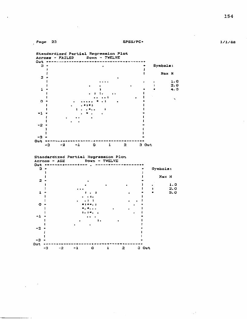
154

Page 23 SPSS/PC*

Standardised Partial Regression Plot Across - FAILED Down - TWELVEOut •*■ +-----*------*-- — -*------ - — • -

3 +

-I

-2

Symbols: Max N

1.02. 04. 0

-3 * Out -

-3 -2 -1 3 Out

Standardised Partial Regression Ploi: Across - AGE Down — TWELVEOut ---. •

3 *

-2

Symbols: Max N

1. O2. 05. O

i / i / a a

-3 - Out -- -3 - 2 - 1 0 1 2 3 Out

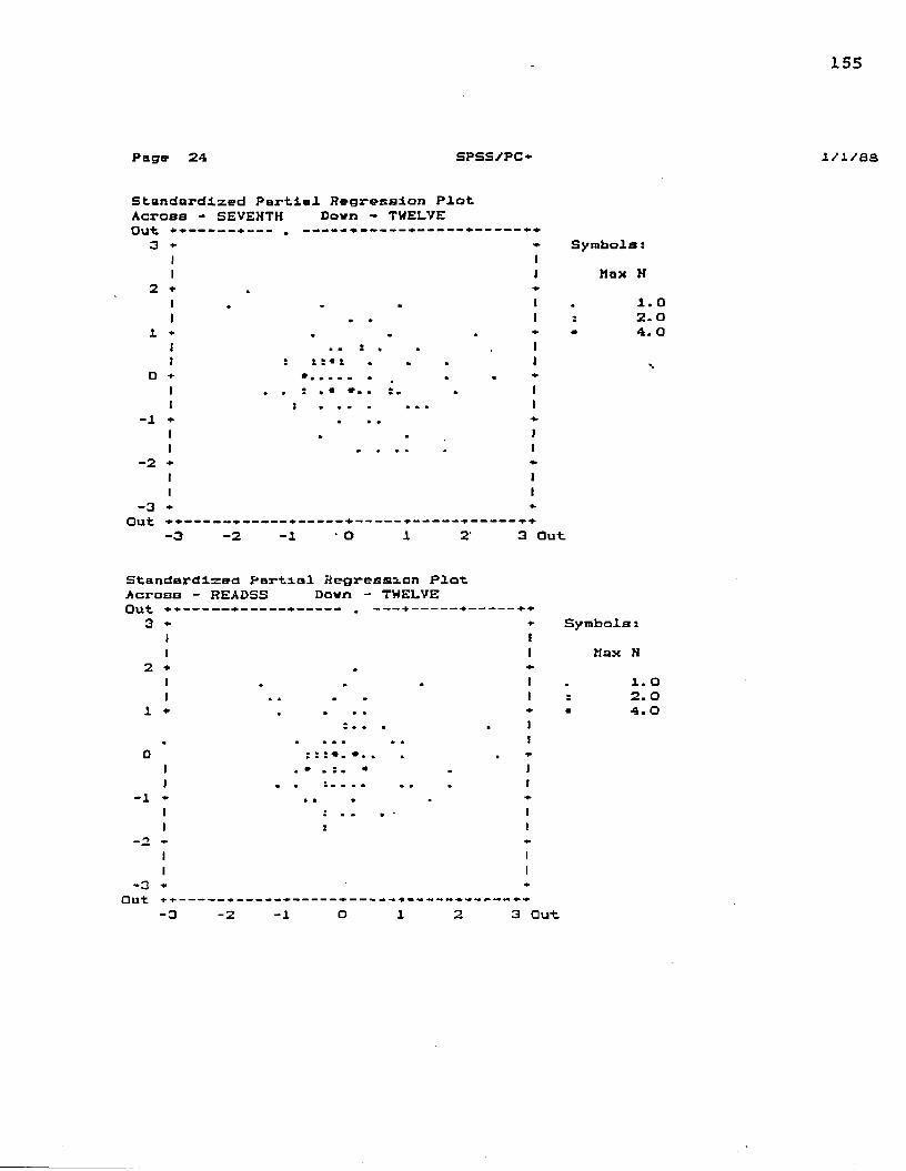
155

Page 24 SPSS/PCi i / i / a s

Standardized Partial Regression Plot Across - SEVEHTH Down - TWELVE

3 +■

-1

-2

Symbols: Max H

1. 0 2. O4. O

-3 - *Out *----- * * +

- 3 - 2 - 1 0 1 2* 3 Out

Standardized partial Regression Plot Across - READSS Down - TWELVE3 *

JI2 +1 . . .I . . .1 . ...

-1

Symbols: Max H

1.0 2. O 4. O

-3 *Out - -

— 3 - 2 - 1 O 1 2 3 Out

156

Page 25 SPSS/PC* i / i / a e

Standardized Partial Regression Plot Across - HOMED Dovn - TWELVEOut ♦ + ----- + , - — — ■* -

3 *II2 ♦

-1-2

Symbols: Mom »

1.02. O4. 0

-3 + Out **■

-3 -2 -1 3 Out

Standardised Partial Regression Plot Across - FIFTH Down - TWELVE

3 +

-1

-2

-3 *Out +-3

Symbols: Max H

1.02. O3. 0

-1 3 Out

157

Page 26 SPSS/PC* 1/A/8B

Standardized Partial Regression Plot Across - SPEDYR Dovn - TWELVE

0 cU 1+

- + ♦ ♦ 1 1 1 1 1 1 1 1 1 1 1 1 1 1 1 1 1 1 1 1 1 1 I 1 1 1

S ymbols:11

2 +1 • »1 : -

1 + a 1 *

Max N1.0

: 2. 0 * 4.0

1 • Z * p *

1 . : i i. 0 +

1 •1 A1 * a • •

-1 + .. :

-2 * 11

-3 *Out --------------

- 3 - 2 - 1 O 1 2♦

3 Gut

Standardized Partial r?grec5l;n Plot Across - ATTEND Dovn - TWELVE

3 +

I

— — ♦ ♦

*

| Symbols :

f

1 *

2 *

1 * , :

i a a e ■ a

1

1

tt1j

Max N1. 0

: 2. 0 3. O

1 • a a a »

J * . a

Q + ............ :1 *

1 - - - - •* * :-i * . .

1 a a • • a

1II1

l a a

-2 ■* *

11

-3 *Out — » - ----------------- + ■ ---------------—1

+

- 3 - 2 - 1 O 1 2 3 Out

158

Page 27 SPSS/PC* 1/1/aa

-3 Out ♦+-

-3

Standardized Partial Regression Plot Across - SIS Down - TWELVEOut — — — * —- — — —

3 * t I

2 *

i. *:

Symbols; Max N

1.02.03. □

-2 3 Out

APPENDIX FDISCRIMINANT ANALYSIS AND PLOTS OF TWELFTH GRADE DATA

159

160

D I S C R I M I N A N T A N A L Y S I S

On groups defined by GROUP group assignment164 (unweighted) cases were processed.S6 of these were excluded -from the analysis.

0 had missing or out-of-range group codes.86 had at least one missing discriminating variable.

73 (unweighted) cases will be used in the analysis.Number of Cases by Group

Number of Cases GROUP Unweighted Weighted

1 20 2 0 .02 24 24.03 IS 15.04 19 19.0

Total 73 73.0

Labelfemale attender male attender female nonattender male nanattender

Group means GROUP 1

24

Total

AGE13.10000 13.20333 IS .1333313.2631619.17949

TWELVE i.76000

11.79533 15.61333 25.64737 14.61232

ATTEND3.75000 3.95333 4.93333 4.315794.17949

RETAIN .00000 .12500 .00000 .10526 .06410

GROUP 1•»4

Total

MOMED12.4500012.0333311.4666712.6342112.20513

DADED13.3000012.0416712.4666712.6342112.60256

SIB 2.25000 1.66667 1.60000 1.15739 1.67949

SPEDYR . 00000 .37500 .00000 .26316 .17949

GROUP 1234

TotalGROUP 1

4Total

GROUP 134

Total

FIFTH 4.17000 3.90000

- Z . 63667 5.78947 4.38946

GPA 2.79200 2■50375 2.14967 1.49737 2.26423

MATHSS572.40000555.75000560.40000 513.52632 551.94615

SEVENTH 5.14000 5.54593 5.66000 5.23634 5•jS946

APTSS49.40000 50,2093349.00000 46.94737 49.97436

NINTH 5.19500 6.84167 7.62667 7.42105 6.71154

READSS 551.95000 590.54167j71, j555.26316 563 - 4 p 4 6

FAILED .95000

2.750004.40000 9.68421 4.29437

LANGSS 561.30000 553.37500 563.95335 512.99474 547.57692

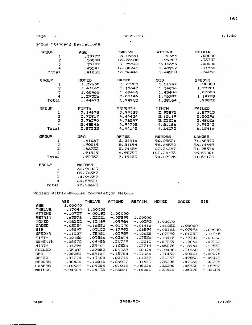
161

Page 3Group Standard Deviations

GROUP I

4Total

AGE.30779 .50998 .35197 .45241 .41952

SPSS / £ ' £ + •

TWELVE 3.65231 13.73680 7.25543

16.90742 13.56446

ATTEND .96655 .99909

2.18654 1.49267 1.44818

RETAIN .00000 . / QnJ.00000 .31530 ,24652

GROUP

4Total

MOMED 1.27630 1.411651.68466 1.29326 1.44473

DADED I.71985 2.156471.68466 2.00146 1.94962

SIB 1.51744 1.34056 1.45406 1.06787 1.38164

SPEDYR .00000

1.27901 .00000

1.14709 .90802

GROUP 1u4

Total

FIFTH 3.14678 2.75917 3.76390 5.48846 3.87325

SEVENTH 3.99189 4.44454 4.76547 4.94708 4.44145

NINTH 2.95875 5.15119 5.33526 4.81186 4.64372

FAILED1.877155.50296 3.48056 7.99342 6.15410

GROUP

4Total

GROUP 1r>

4Total

GPA.61067 .90519 .66733 .91849 .92352

MATHSS 66.96063 89.76552 74.96552 66.55521 77.28663

APTSS 6.24416 8.SI194 5.74456 6.98788 7.19483

READSS 90.28521 96.64592 62.36467 102.34193 90.69225

LANGSS 71.68873 96.14699 81.25574 65.59801 81.51130

Pooled Within-Graups Correlation Matri;AGE TWELVE ATTEND RETAIN MOMED DADED STB

AGE 1.00000TWELVE .17044 1.00000ATTEND 10737 -.00193 1.00000RETAIN .63576 .22021 -.05899 1.00000MOMED -.08352 -.12069 .09984 -.10292 1.oooooDADED -.05254 -.16850 -.01040 -.01416 .61283 1.00000SIB .09897 .03152 17993 .06894 -.08406 -.07996 1.00000SPEDYR -.11227 .38081 .03989 -.10033 -.02290 -.01383 .11215FIFTH -.00050 .03866 02674 .27536 -.10415 -.12704 -.00336SEVENTH -.08572 .0445B .20749 . 12212 -.02259 -.12064 .09348NINTH .0^794 .59404 .15530 .27714 -.05878 -.13964 .12557FAILED .350S7 .67852 .04469 .40024 -.20400. -.31063 .02185GPA -.23253 -.59164 -. 15784 — .32066 .31454 .40441 -.00275APTSS .07274 -.13408 .02715 .11347 .24257 .49556 -.09342READSS .00430 -.12816 —. 06037 .01633 .25305 .47162 -.03720LANGSS -. 10568 -.05255 .01014 -.08236 .26380 .45938 -.19922MATHSS -.04500 -.24436 -. 06871 -.19263 .23848 .45828 -.04480

1/1/30

-age 4 SPSS/PC-i- 1/1/80

162

Page 4 SPSS/PC■+• 1SPEDYR FIFTH SEVENTH NINTH FAILED GPA APTSS

SPEDYR 1.00000FIFTH .19933 1 . 00000SEVENTH .41697 .42501 1.00000NINTH .34577 .34542 .48933 1.00000FAILED .20659 .10445 .10140 .51867 1.00000GPA -.25725 -.09210 -.15191 -.47561 -.79417 1 . 0 0 0 0 0

APTSS -.12447 .058B7 -.06510 -.20491 -.21619 .43737 1 . 0 0 0 0 0

READSS -.23874 -.06323 -.23410 -.17930 -. 19501 .50502 .62180LANGSS -.13710 06909 — .2B694 -.24592 -.27859 .45342 .73710MATHSS -.23037 -.22429 -.27975 — .31956 — . 39353 .61266 .63897

READSS LANGSS MATHSSREADSS 1 . 0 0 0 0 0 V

LANGSS .64515 1 . 00000MATHSS .54248 .62803 1 . 0 0 0 0 0

1/1 / B O

Correlations which cannot be computed are printed asWilks' Lambda (LJ-stati stic) and univariate F-ratia with 3 and 74 degrees of -freedomVariable Wilks' Lambda Signi-fieanceAGETWELVEATTENDRETAINnCIMEDDADEDSIBSPEDYRFIFTHSEVENTHNINTHFAILEDGPAAPTSSREADSSLANGSSMATHSS

.97692

.73315

.91491

.94337

.91229

.93958

.91987

.96569

. 95554.

.99778

.95373

.71433

.72102

.97034

.96740

.93354 ,93259

.5828 S.SB7 2.294 1.481 2.371 1.586 ■2. 149. B7631. 14B.54S8E—011.0629.8649.544.7541.83111.6151.783

.6292

.0000

.0849

.2267

.0772

. 1999

. 1013

. 4574

. 3356

.9829

.3706

.0000

.0000

.5235

.4810

. 1931

. 1578

163

Page S SPSS/PC+ 1/1/SO

D I S C R I M I N A N T " A N A L Y S I S --------------- --On groups defined by GROUP group assignmentAnalysis number 1Stepwise variable selection

Selection rule: Minimise Wilks' LambdaMaximum number of steps...................... 34Minimum Tolerance L e v e l ..........................00100Minimum F to enter............... 1.0000Maximum F to r e m o v e ...................... 1.0000 x

Canonical Discriminant FunctionsMaximum number of functions................ 3Minimum cumulative percent of variance... 100.00 Maximum significance of Wilks' Lambda.... 1.0000

Prior probability for each group is .23000------------------- Variables not in the analysis after step 0

Variable ToleranceMinimum

Tolerance F to enter Wilksi' LambdaAGE 1.0000000 1.ooooooo .38279 .97692TWELVE 1.0000000 1.ooooooo 8.8B65 .73315ATTEND 1.0000000 1.0000000 2.2940 .91491RETAIN i.ooooooo 1.ooooooo 1.4808 .94337MOMED 1 .ooooooo 1.ooooooo 2.3714 .91229DADED 1.ooooooo 1.0000000 1.3861 .93958SID 1 .ooooooo 1.0000000 2.I486 .91987SPEDYR 1 .ooooooo 1 .ooooooo .87627 .96569FIFTH 1 .ooooooo 1.ooooooo 1.1478 .95554SEVENTH 1.ooooooo 1.ooooooo .54S78E— 01 .99778NINTH 1.ooooooo 1.0000000 1.0619 .95873FAILED 1.ooooooo 1.ooooooo 9.B643 .71433GPA I.ooooooo 1.0000000 9.5443 .72102APTSS 1.ooooooo 1.0000000 .75411 .97034READSS 1.ooooooo 1.0000000 .83112 .96740LANGSS 1.ooooooo 1.ooooooo 1.6132 .93854MATHSS 1.ooooooo 1.0000000 1.7831 .93259K x * * * * * * * * * * * * t * % i i i i * t i * * * S XAt step 'l, FAILED was included in the analysis.

Degrees of Freedom Signif. Between Groups Wilks' Lambda .71433 1 3 74.0Equivalent F 9.96431 3 74.0 .0000 Variables in the analysis after step 1 -------------------Variable Tolerance F to remove Wilks' LambdaFAILED 1.0000000 9.9643

164

Page 6in

S P S S / F Othe analysis after step

Variable ToleranceMinimum

Tolerance F to enter Wilks’ Lambd.AGE .0760927 .0760927 .44434 .70152TWELVE .5396077 .5396077 1.0421 .60500ATTEND .9980025 .9980025 1.9810 .66054RETAIN .0390O64 .8398064 1.9189 .66212MOMED .9583829 .9583029 3.1401 .63250DADED .9034792 .9034792 2.1841 .65550SIB .9995225 .9995225 1.7407 .66665SPEDYR .9573210 .9573210 .91407 .60045FIFTH .9890899 ,9890099 .56330 . 6981,7SEVENTH ■ .9897175 .9897175 .13545 .71030NINTH .7309862 .7309862 1.4697 .67365GPA .3692944 .3692944 .90667 .68B67APTSS .9532600 .9532600 .15098 .70970READSS .9619715 .9619715 .90207 .6SBS0LANGSS .9223902 .9223902 .356S0 .70401MATHSS .8451355 .8451355 .13490 .71039X * * * t « * & * * * t > M t * * * * * * X * x * x X * i

1/1/00

At step 2, HOMED was included in the analysis..

Milks' Lambda Equivalent F

Degrees of Freedom Signif. .63250 2 3 74,0

6.26303 6 146,0 .UOUOBetween Groups

Variables in the analysis after stepVariable Tolerance F to remove MOMED .9363829 3.1401FAILED .9503B29 10.764

Milks' Lambda .71433 .91229

Variables not in the analysis after stepMini mum

Vari able Tolerance Tolerance F to enter Wilks' LambdAGE .0767439 .0461591 .42911 .62139TWELVE .5392796 .5244755 1.0011 .60718ATTEND .9856154 .9464875 2.2119 .57913RETAIN .0393344 .8130156 1.3774 .50662DADED .5884785 .5884705 1.0530 .50717SIB .9929105 .9520430 1.6350 .59214SPEDYR .9569353 .9175916 .90725 .60947FIFTH .9819280 .9513041 .71376 .61424SEVENTH .9897137 .9490092 * .11896 .62930NINTH .7286786 .7007744 1.5156 .59493GPA .3450205 .3450205 1.1766 .60294APTSS .9121613 .9121613 .41075 .62166READSS .9145138 .9111021 1.2241 .60131LANGSS .8776965 .0776965 ,07606 .61023MATHSS .8190200 .8190200 .33962 .6236a

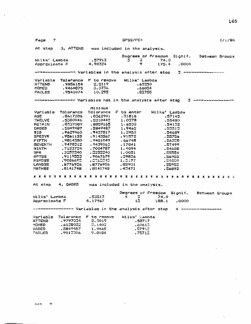
165

Page 7 At step j j ATTEND

SPSS/PC+* was included in the analysis.

Degrees of Freedom Signif.Wilks' Lambda .57913 3 3 74.0Approximate F 4.90324 9 175.4 .0

the analysis after step 3 •Variable Tolerance F to remove Wilks' LambdaATTEND .9856154 2.2119 .63250MQMED .9464Q75 3.3736 .66054FAILED .9541074 10.295 ■82755

in the analysis after stepMi ni mum

Variable Tolerance Tolerance F to enter Wilks' Lambd;AGE .S6171B6 .8362901 .31816 .57145TWELVE .5380946 .5210442 1.0378 .55480RETAIN .8337089 . 8059165 1.6530 .54132DADED .5B49487 .5849487 1.9465 .53512SIB .9629460 . 9427S17 1.3953 .54689SPEDYR .9561133 . 9143567 .91572 .55756FIFTH .9S14380 . 9401049 .66748 .56325SEVENTH .9478312 . 9439063 .17041 .57499NINTH .7123724 .7004787 1.4094 .54658GPA .3252240 . 3252240 1.0051 .55554APTSS .9119553 .9067679 .39826 .56955READSS .'90S6692 . 2 ”763313 1.3177 .54539LANGSS .8776956 .8776956 .82901 .55953MATHSS .S14174S .8141748 .42471 .56892* * * * •t * * * * * * * * * * * X * * * * * * * * * * * * *At step 4, DACED was included in the analysi s.

Degrees of Freedom Signi

1/1/30

Between Groups

Wilks' Lambda Approximate F

.53512 4.17967

s>12

74.0 1SB. 1

Between Group;.0000

------------------- Variables in the analysis af ter stepVariable Tolerance F to removeATTEND .9797034 2.3019MDMED . 6128022 3.14030ADED .5B494S7 1.9465-AILED .9012306 9.S1B4

Wilks' Lambda .58717 .60613 .57913 .75712

r.nra O

166

Page SPSS/PC+ l/i/eoVariables not in the analysis after step

Mini mumVariable Tolerance Tolerance F to enter Wilks' LambAGE .8563518 . 5813056 .40170 .52606TWELVE .5365466 .4979318 1.0240 .51262RETAIN .8099363 .5682693 2.1469 .49003SIB .9605004 .5834631 1.4193 .50444SPEDYR .9532368 .5831888 .97596 .51364FIFTH .9774322 .5825612 .67799 .52001SEVENTH .9379863 .5788729 .12104 .53236NINTH .7084542 .5817314 1.3217 .50643GPA .3186782 .3186782 1.0892 .51126APTSS .7418257 .4758237 1.2817 .50726READSS .7705602 .4960421 2.4589 .48410LANG8S .7673000 .5113744 .91200 .51499MATHSS .7147322 ■ 5135035 .31835 .52792* * * * * * * * * * * * * * * * * * * * * * * * * * * * *At step 5, READSS was included in the analysi s.

* * * * * * * * * * *

Milks' Lambda Approximate F

.48410 3.S8000

Degrees of Freedom Signif. 5 3 74.0

15 193.6 .0000Between Groups

Variables in the analysis after steDVari ableATTENDK0MEDDADEDFAILEDREADSS

To!erance .9768506 .6115571 .4960421 • 6983645 .7705602

F to remove 2.3145 3.0973 3.1080 9.5832 2.4589

Milks' Lambda .53212 .54837 .54859 .68293 .53512

Variables not in the analysis after stepMi ni mum

Variable Tolerance Tolerance F to enter Wilks' LambAGE .8544000 .4945811 .32744 .47731TWELVE .5361698 .4942736 1.0260 .46343RETAIN .8082473 .4864920 1.9108 .44697SIB .9603685 .4951727 1.3352 .45754SPEDYR ,8901552 .4842379 1.6688 .45136FIFTH .9774231 .4943925 .64739 .47085SEVENTH .9041890 .4958293 .19937 .47994MI NTH .7044434 .4952736 1.4045 .45624SPA .2202613 .2202618 2.0860 .44385^PTSS .5511718 .4594220 .39358 .47596-AN8SS .5370421 .4833204 .82452 .46735■IATHSS .5916042 .4770203 .29565 .47796

167

Page ‘ At step 6, GPA

Milks’ Lambda Approximate F

SPSS/PC+ was included in the analysis.

Degrees of Freedom Signif. .443SS 6 3 74.0

3.61593 19 195.6 .0000Variables in the analysis after step

VariableATTEND.MGMEDDADEDFAILEDGPAREADSS

To!erance .9197964 .5953466 .4909493 .2921033 .2202618 .5325905

F to remove1.9773 3.3956 3.21B7 .70995 2.0960 3.4930

Milks’ Lambda .48009 .50918 .50596 .45755 .49410 .51126

Variables not in the analysis after step Minimum

Vari able Telerance Tolerance F to enter Wilks' LambdAGE .9474897 .2184804 .37691 .43659TWELVE .5211398 .2140870 .57060 .43295RETAIN .9025799 .2197174 1.9566 .40891SIB .9599659 .2201466 1.1403 .42259SPEDYR .8887231 .2199075 1.6194 .41425FIFTH .9772013 .2202118 • 64313 .43160SEVENTH .9016999 .2196552 . 18053 .44034NINTH .7003091 .2191236 1.4763 .4 « * * 7 ’

APTSS .5315377 .2124156 .30410 .43797LANGSS .5349072 .2193862 .65SS4 .43131MATHSS .5153902 .1918864 . 14943 .44094* * * * * * * * * * * * * * * * * * * * * * * * * * * * * :At step 7 ■, FAILED was removed from the analysi s.

1/1/80

Between Groups

* * * * * * * * * *

Milks' Lambda Approximate F

Degrees of Freedom Signif. .45755 5 3 74.0

4.22665 15 193.6 .0000Between Grouos

------------------ Variables in the analysis after stepVariableATTENDMOMEDOADEDGPA4EADSS

Talerance .9437091 .5939813 .5100569 .6774159 .6532536

F to remove 2.0455 3.6955 2.952711.494 3.5357

Milks’ Lambda .49766 .5o001 • 51545 .68293 .52683

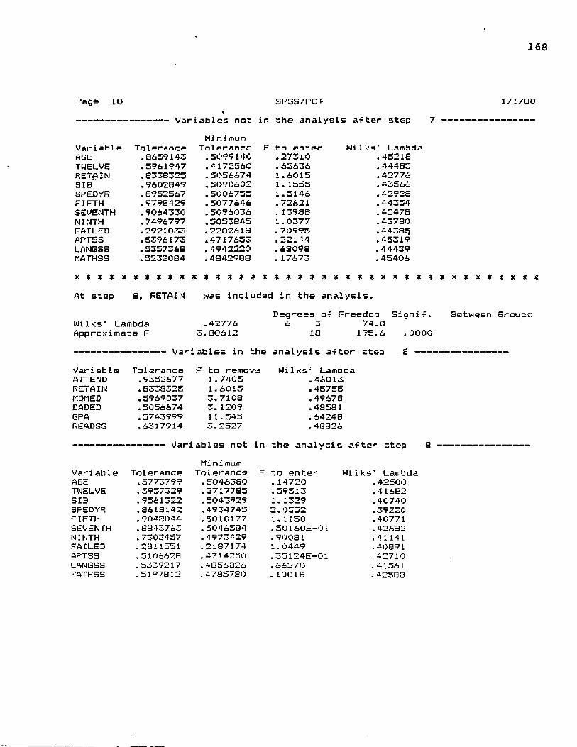
Page 10 SPSS/PC+*

Variables not in the analysis after step 71/1/80

MinimumVariable Tolerance Tolerance F to enter Wilks' LambiAGE .8659143 .5099140 .27310 .45218TWELVE .5961947 .4172560 .656o6 .44485RETAIN .8338325 .5056674 1.6015 .42776SIB .9602849 .5090602 1.1555 .43566SPEDYR .8952567 .5006755 1.5146 .42928FIFTH .9798429 .5077646 .72621 .44354SEVENTH .9064330 .5096036 .13938 .45478NINTH .7496797 .5053845 I.0377 .43780FAILED .2921033 .2202618 .70995 .44385APTSS .5396173 .4717653 .22144 .45319LANGS5 .5357368 .4942220 .68098 .44439MATHSS .5232084 .4842988 .17673 .45406* * * * * * * % X * * X * # # # X X X X X x x x x x x x xAt step B, RETAIN was included in the analysi s.

* X X * t ■ * * * * * %

Wilks' Lambda Approximate F

Degrees of Freedom .42776 6 3 74.0

3.80612 18 195.6— Variables in the analysis after step

Signi f .. 0000 a --------

Between Groups

VariableATTENDRETAINMOMEDDADEDGPAREADSS

Tolerance .9352677 .8358325 .5969037 .5056674 .5743999 .6317914

F to remove 1.7405I.6015 3.7108 3.1209II.545 3.2527

Wil*<&: Lambda.46013 .45755 .49678 .48581 .64248 .48826

Variables not in the analysis after step

Variabl e AGETWELVESIBSPEDYRFIFTHSEVENTHNINTHFAILEDAPTSSLANS5S■IATHSS

Tolerance .5773799 ,5957329 .9561322 .8618142 .9048044 ,8843763 .7303457 .2811551 .5106628 .5339217 .5197812

Mi ni mum Tolerance .5046380 .3717785 .5043929 .4934745 .5010177 .5046584 .4973429 .2187174 .4714250 .4856826 .4735780

to enter .14720 .59513 1.1329 2.0552 1.1150 .5016OE-01 .90081 1.0449 .35124E—01 .66270 .10018

Wilks' Lambda .42500 .41682 .40740 .39220 .40771 .42682 .41141 .40891 .42710 .41561 .42588

169

Page 11 SPSS/PC+ l/l/SOAt step 9, SPEDYR was included in the analysis.

Degrees of Freedom Signif. Between Croups Wilks’ Lambda .39220 7 3 74.0Approximate F 3.59319 21 195.S .0000

Variables in the analysis after stepVariableATTENDRETAINMOMEDDADEDSPEDYRGPAREADSS

Tolerance .9345066 .0026845 .5966544 .4934745 .3610142 .5385108 .6189052

to removeI.6796 2.1429 3.6598 3.6162 2.0552II.947 3.4268

Wilks’ Lambda .42126 .42928 .45553 .45477 .42776 .59892 .45150

Variables not in the analysis after step Minimum

Variable Tolerance Tolerance F to enter Wilks' LambdaAGE .5720505 .4930356 .73078E—01 .39092TWELVE .5244517 .3717764 1.2214 .37186SIB .9370476 .4909069 1.2695 .37111FIFTH .0393560 .4836981 1.8086 .36282SEVENTH .7133202 ,4858556 .29713 .38705NINTH .6504050 .4793307 1.0063 .37529FAILED .2765758 .2179494 1.3141 .37041APTSS .5080968 .4631505 .73746E-02 .39207LANGSS .5337900 .4771554 .65742 .38099MATHSS .5123280 .4632428 .49986E-01 .39133* * * * * * * * * * * * * * * * * * * * * * * * * * * * * *At step 10, FIFTH was included in the analysis.

* * * * * * * * * *

Wilks’ Lambda Approximate F

Degrees of Freedom Signif. .36282 8 3 74.0

3.39856 24 194.9 .0000Between Groups

Variables in the analysis after step 10Variable Tolerance F to removeATTEND RETAIN .MOMED DADED 5PEDYR FIFTH GPAREADSS

.9344361

.7162742 ■ 59665^2 .4836981 .7994755 • 8393560 .5287232 .6189850

1.6525 3.0075 3.5796 3.9229 2.7631 1.8086 12.400 3.3671

Wilks’ Lambda .38967 .41168 .42097 .42655 .40771 .39220 .56427 .41752

170

Page 12 SPS5/PC+ 1/1/80in the analysis after, step 10

Mi ni mumVari able Tolerance Tolerance F to enter Wilks' LambdaAGE .5429145 .4656727 .17669 .35993TWELVE .5176577 .370S477 1.4369 .34058SIB .9309056 .4003673 1.2618 .34314SEVENTH .6275888 .4006104 .26214 .35855NINTH .6047197 .4674572 1.4503 .34038FAILED .2761814 .2172322 1.3107 .34242APTSS .5023742 .450S797 .46562E—01 .36205LANGSS .5337454 .4687139 .64647 .35246MATHSS .4975210 .4530364 .95253E-01 .36126* * * * * * * * * * * * * * * * * * * * * * * * * * * * * * * *At step 11, NINTH was included in the analysis.

Milks' Lambda Approximate F

Degrees of Freedom Signif. 13403S 9 3 74*0

3.19675 27 193.4Variables in the analysis after step

. 0000 1 1 ---

Between Groups

Variable Tolerance F to remove W i 1ks’ LambdaATTEND .9232931 1.3240 .36007RETAIN .7021317 2.8132 .38391MDMED .5818607 4.0315 .40276DADED .4746989 3.o“0° .40120SPEDYR .7427843 2.4S39 .37001FIFTH .7803905 2.2563 .37529NINTH .6047197 1.4503 .36202GPA .4674572 13.226 .54501READSS .609460S 3.4631 .39396

Minimumthe analysis after step

Variable Tolerance Tolerance F to enter Wilks' LambdaAGE .5253748 .4433469 .23342 .33675TWELVE .4182622 .3689917 2.7095 .30255SIB .9105209 .4599942 1.0694 .32437SEVENTH .5540437 .4376808 .41237E—01 .33973FAILED .2627743 .2163315 1.6469 .31634APTSS .4926433 .4466225 .10707 .33871LANGSS .5272632 .4624000 .81549 .32303MATHSS .4966921 .4033823 .10093 .33000

11

171

Page 13 SPSS/PC+ 1/1/30

At step 12, TWELVE was included1 in the analysis.Degrees a-f Freedom

Nilks’ Lambda .30255 10 3 74.0Approximate F 3.20370 30 191.5

analysis a-f ter stepVariable Tolerance F to remove Wilks' LambdaTWELVE .4182622 2.7095 .34038ATTEND .8332699 1«oo5o .32119RETAIN .7019279 2.6642 .33975MOWED .5313900 3.798B .35559DADED .4737639 3.9218 .35731SPEDYR ■ 6564 15 7 3.1707 .34632FIFTH .7337631 3.1650 .34674NINTH .4886074 2.7234 .34053GPA .36B9917 .34938READSS .563S384 2.7346 .34073

Between Groups.0000

12

Variables not in the analysis aFter step Minimum

12

Variable Tolerance Tolerance F to enter WiLks’ LambdaAGE .5250274 .3604699 .22512 .29939SIB .9005171 .3674192 .99891 .28901SEVENTH .4925026 .3664358 .43692 .29647FAILED .2416006 .2116015 .86323 ' .29078APTSS .4S0607S .3500037 .2916.9 .29847LANGSS .4744824 .3501413 1.7129 .28006MATHSS .4841284 .3108239 .2128IE-01 .30224* # * * * % t * * * * * # * # * *At step 13, LANGSS was included‘ in the analysis.

Degrees of Freedom Signi-f.Wilks’ Lambda .28006 11 3 74.0Approximate F 3.09891 33 139.3 .0000---------- — ------ Variables in the analysis a-f ter step 1 3 -----Variable Tolerance F to remove Wilks' LambdaTWELVE .3763928 3.6545 .32003ATTEND .8589932 1.2587 .29658='ETA IN .7004364 2.6565 .31493•10MED .5310449 3.4211 .32497DADED .4578305 3.5881 .327163FEDYR .6347695 3.1610 .32156- IFTH .7232441 3.4271 . - ■ i O«—i■ilNTH .4596032 3.5475 -326633PA ■ 3501413 1.9900 .30618*:EADSS .4601S2O 3.1300 .32115.ANGSS .4744S24 1.7129 .30255

Between Groups

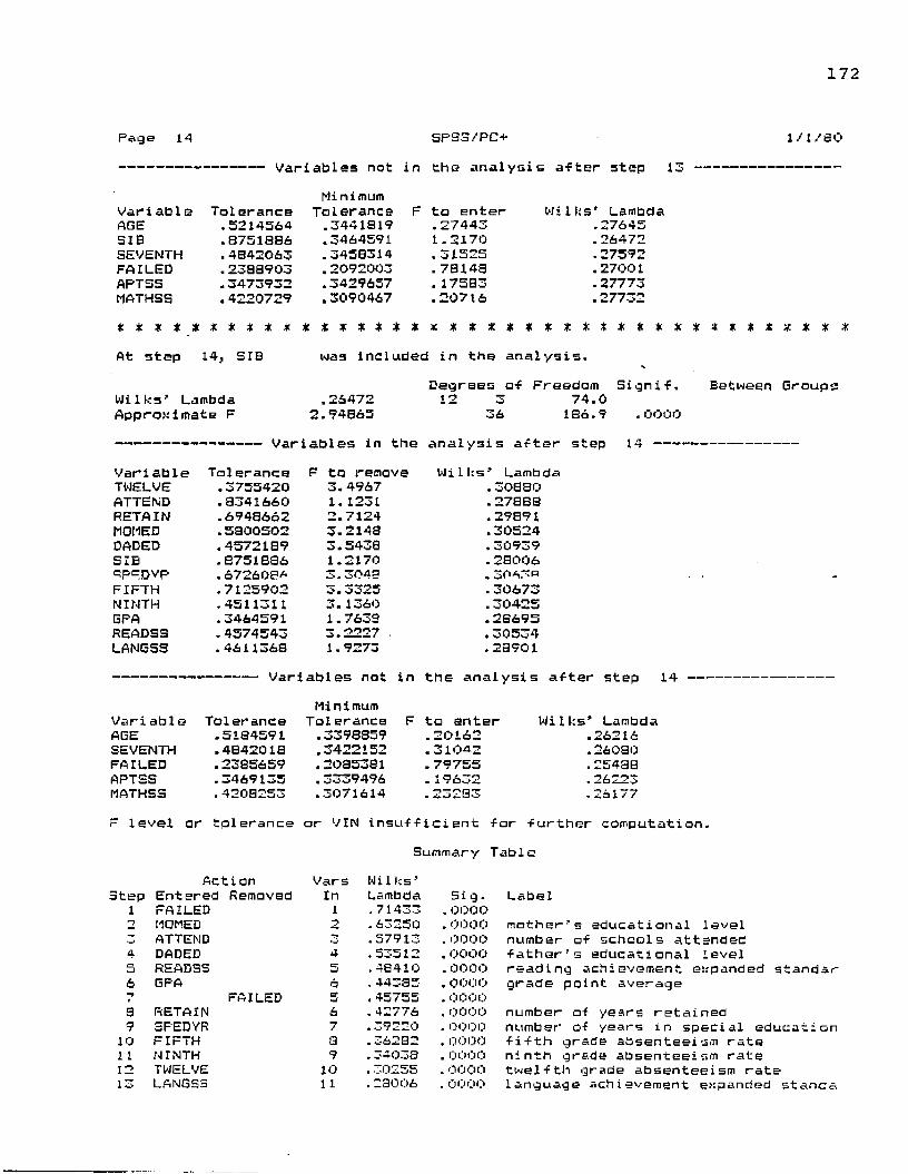
172

Page 14 SPSS/PC+Variables not in the analysis after step 13

Minimum

l/i/eo

Vari able Tolerance Tolerance F to enter Wilks' LambdaAGE .5214564 .3441819 .27443 .27645SIB .8751886 .3464591 1.2170 .26472SEVENTH .4B42063 .3450314 .31525 .27592FAILED .2388903 .2092003 .78148 .27001APTSS .3473932 .3429657 .17583 .27773MATHSS .4220729 .3090467 . 20716 .27732* * * * * * * * * * * * * * * * * X X * * * * * * * * * * * *At step 14, SIB was included in the analysis.

Degrees of Freedom Signif,Wilks' Lambda .26472 12 3 74.0Approximate F 2.94865 36 186.9 .0000

iables in the i n 1 t , rt h r* I, h m p. *» n n 1 /I _ _ —ctrictiysis step 1

Variable Tolerance F to remove Wilks' LambdaTWELVE .3755420 3.4967 .30880ATTEND .8341660 1.1231 .278BSRETAIN .6948662 2.7124 .29891MOMED .5800502 3.2148 .30524DADED .4572189 . .j4o 0 .30939SIB .S7518S6 1.2170 .28006qpcjjvp .6726084 3.3045 .304“nFIFTH .7125902 3.3325 .30673NINTH .4511311 3.1360 .30425GPA .3464591 1.7638 .28695READSS .4574543 3.2227 • .30534LANGSS .4611368 1. 9273 .28901

the analysis after step 14Minimum

Vari able Tolerance Tolerance F to enter Wilks' LambdaAGE .5184591 .3398859 .20162 .26216SEVENTH .4842018 .3422152 .31042 .26080FAILED .2385659 .2085381 .79755 .25488APTSS .3469135 .3339496 .19632 .26223MATHSS .4208253 .3071614 .23283 .26177F 1evel ar tplerance or VIN insufficient for further computati

Between Groups

Summary TableAction Vars Wilks’

Step Entered Removed In Lambda Sig. Label1 FAILED 1 .71433 . OOOO<”7 MOMED .63250 . 0000 mother’s educational level

ATTEND o .57913 . 0000 number of schools attended4 DADED 4 .53512 . OOOO father’s educational level5 READSS 5 .48410 . OOOO reading achievement expanded standar6 GPA 6 .44385 . 0000 grade point average-T FAILED 5 .45755 . 00008 RETAIN 6 ,42776 . 0000 number of years retained9 SPEDYR 7 .39220 . oooo number of years in special education10 FIFTH a .36282 . oooo fifth grade absenteeism rate1 1 NINTH 9 . j 40^>8 . oooo ninth grade absenteeism rate12 TWELVE 10 .30255 . oooo twelfth grade absenteeism rate13 LANGSS i i . 28006 . oooo language achievement expanded stanca

f 173

Page IS SPS3/PC+ l/l/SO14 SIB 12 .26472 .0000 number of siblings residing in home

Canonical Discriminant FunctionsPet of Cum Canonical After Wilks1

Fen Eigenvalue Vari ance Pet Corr Fen Lambda Chisquare DF Sig: 0 .2647 91.707 36 .OOOO

1* 1.1010 61.SB 61.53 .7239 : 1 .5562 40.480 ”>n .00952* .4260 23.33 83.41 .3466 : +2 .7931 15.995 10 . 09903* .2609 14. 39 100.00 .4349 :* marks the o canonical discriminant functions remaining in the analysis.

Standardized Canonical Discriminant Function CoefficientsFUNC l

TWELVE -.84054ATTEND -.10179RETAIN .29519MOMED -.3102aDADED -.20243SIB .14643SPEDYR .30521FIFTH -.524B7NINTH .68872GPA .65557READSS -.36803LANGSS .33780

FUNC 2 FUNC 3-.17538 .05453-. 16867 -.47626.61100 .13953.48714 .71205

-.99253 -.0059a-.33862 .17365.71347 . 07874

-.32032 .28811-.06477 -.42961.08257 .21896.79001 -.40191

-.28803 -.16948Structure Matrix:Fooled—within—groups correlations between discriminating variables

and canonical discriminant functions (Variables ordered by size of correlation within function)

FUNC 1 FUNC 2 FUNC 3SPA .57215* -.08465 .29904TWELVE -. 55029* .14105 26546FAILED -.54307* .25912 -.27275MATHSS .33564* -,15757 .00763SIB .23420* -.18544 .21509LANGSS .22319* -.09713 -.12586FIFTH -. 13910* .00467 .16558APTSS . 10352* -.02343 -.02900RETAIN 07657 .35173* .05801DADED -.00832 32346* .27449SPEDYR -.03791 .280B3* .03650AGE -.13192 .27705* .06373READSS .07400 .21974* 16492SEVENTH .09924 .11902* -.01735MOMED -.13790 ,02377 .53604*ATTEND 11315 -.11219 — .53093*NT NTH -.11344 .11065 -.30118*

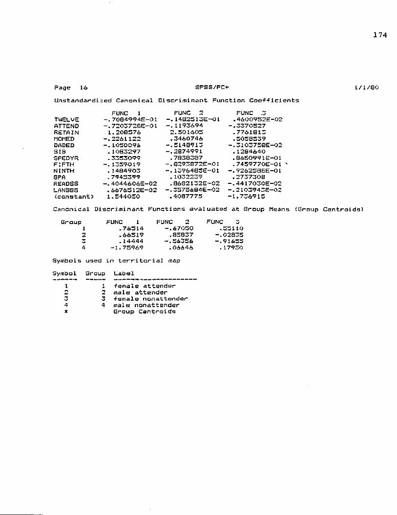
174

Page 16 SPSS/PC+-Unstandardiced Canonical Discriminant Function Cae-f -f ici ents

1/1/ao

TWELVEATTENDRETAINMOMEDDADEDSIBSPEDYRFIFTHNINTHGPAREADSS LANGSS (constant)

FUNC 1 70B4994E-01

-. 7203728E-01 I.208576 2261122 1050096

.1083297

.3353099 -. 1359019 .1484903 .7945399 -. 4044606E—02 .6676512E—02 1.544050

FUNC 2 14B2S13E—01

-. 1193694 2.501605 .3460746 -.5148913 -.2874991 .7830387 8293S72E—01 1396485E—01

.1032239

.8632132E—02 ■. 3575684E—02 .4087775

FUNC ,3 .4600952E—02

— .3370527 .7761813 .5058539

— .3103758E—02 . 1284640 .865099lE-Ol . 7459770E—01

— . 92625BGE—01 .2737308

— .4417030E—02 — .2103943E—02 -1.736915

Canonical Discriminant Functions evaluated at Group Means (Group Centroids) Group FUNC 1

.76514

.66519

.14444 -1.75969

FUNC 2 -.67050 .85837

-.56356 .06646

FUNC 3 .55110

-.02835 91655

.17930Symbols used in territorial map Symbol Group Label

1

4*

1 -female attender2 male attender3 -female nonattender4 male nonattender

Group Centroids

o. n

175

17

n0 n1 c a 1Diacrimin-antFuncti□n

SPSS/PC+ Territorial Map * indicates

(assuming all -functions but thea group centroid first two are :erol

- 6.0+ -

6.0 +

-4.0

4.0 +

2.0

- 2.0

-4. 0 +

4.0Canonical Discriminant Function

- 2.0 .0 2.04424224422442422442+422 + + +442422442422442

+ 422 + + +4422 442 422 X442

11111111 4333311111111111111111

443 3*1 *433 31

6-0

H 111+

443 4433 433

443 433

443

331311 31

331 311 31

- 6.0 + +- - 6.0 -4. 0

4 3 3 31443 331

+433 311 + + +443 31

4433 331433 311

443 314uo 31

443 331

1 l-J O ■

. 0 2.0

1y 0 a . t j

i/i/ao

C T)

C -fj

176

can□nica1Discrimi

FLlnction

OutX-

□ut X'4.0

Canonical Discriminant Function 1-2.0 .0 2.0 4.0 Out

-XX

4.0

.0

- 2.0

-4.0

I+

r>4 2 3 2

4 r> <7 24 22 43

4 3 1 22 1 34 * 44 434 213 21

4 4 33 1 1 1 1 1 34 4 - 4 *

34

X 132 1 2 11 1

Out XX-Out -4. 0 -2.0 .0 2.0 4.0

X-XOut

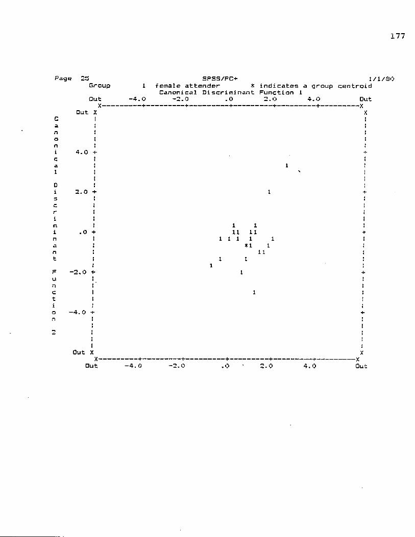
177

Page 25Group

Can0 n1 c a 1Discriminant

unction

SPSS/PC+ 1/1/30female attender # indicates a group centroidCanonical Discriminant Function 1

'2.0 .0 2*0 4*0 Out-XX

- 2,0

-4.0

Out

178

Page 26Group

Can□nica1

scriminan>Function

SPSS/RC-*- 1/1/aomale attender * indicates a group centroidCanonical Discriminant Function 1

-2*0 *0 2-0 4.0 Out*XX

Out X

179

^ageGroupOut

X-Out X

-4.0

SPSS/PC+ i / i / a o-female nonattender * indicates a group CEntroid Canonical Discriminant Function 1

-2.0 .0 2.0 4.0 Out------- +--------- +•--------- +--------- x

Xan3ni 4.0 +a1Di 2.0

1.IDinant

unctiDn

-2, 0I+

-4.0

Out XX-

Out -4.0 -2.0 . 0 2. 0 4.0X

“XOut

lao

Page 2BGroup

can0 n1 c a 1DiscriminantFunction

“4, 0

SPSS/PC+ 1/1/BOmale nonattender # indicates a group centroidCanonical Discriminant Function 1

-2*0 .0 2.0 4*0 Qut

181

a c : l > i u l l l - V K i i U i (.13

No. of Predicted Group MembershipActual Group Cases 1 2 4

Group 1 female attender

23 16 69. 67.

417. 47.

313.07

0.07.

Group 2 male attender

25 624. 07.

1560.07. 8,07.

28.07.

Group 3 female nonattender

19 315.87.

315.BX

947. 47.

421. 17.

Group 4 male nonattender

22 14.57. 9. VA

413. 27.

1568.27.

Percent of "grouped" cases correctly classified: 61.BOX'-Classification Processing Summary

164 Cases were processed.0 Cases were e::eluded for missing or out-of—range group cades.

75 Cases had at least one missing discriminating variable.B9 Cases were used for printed output.

Page 30 3PSS/FC+ 1/1/BO

APPENDIX GMULTIVARIATE ANALYSIS OF VARIANCE ON STUDENT SATISFACTION AND GRADE POINT AVERAGE BY GROUP ASSIGNMENT ON TWELFTH GRADE DATA

182

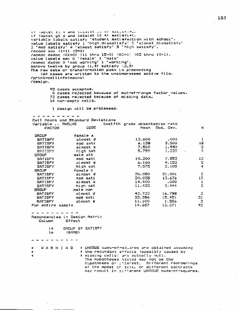
ir \aqLST: it ‘r «nu LuUaist . 5®i.,=.t .s.,if (aptst gt 6 and tatalst It 4> satisfy®!.variable labels satisfy ’student satisfaction with school1', value labels satisfy 1 ’high dissatisfy’ 2 'almost dissatisfy’3 'mad satisfy’ 4 ’almost satisfy’ 5 'high satisfy’, recode sen (1=1) (2=0)/momnc dadoc (01=0) (11 thru 15=0) (OC^l > (02 thru 10=1).value labels sen 0 'female’ 1 'male'/momoc dadoc 0 'not working’ 1 ’working’, manova twelve by group (1,4) satisfy : 2,5)The raw data or transfarmation pass is proceeding

164 cases are written to the uncompressed active file. /print=cel1 info(means)/design.

92 cases accepted.0 cases rejected because of out—of—range factor values.

72 cases rejected because of massing data. s14 non-empty cells.1 design will be processed.

Cell Means and Standard DeviationsVariable .. TWELVE twelfth grade absenteeism rate

FACTOR CODE Mean Std. Dev.GROUP female aSATISFY almost d 13.600 .000SATISFY mod sati 6. 12S 3.300SATISFY almost s 7.500 1.980SATISFY high sat 5.750 ■*

GROUP male attSATISFY mod sati 10.200 7.552SATISFY almost s 6. 160 4. 153SATISFY high sat 7.575 2. 105

GROUP female nSATISFY almost d 30.050 21.001SATISFY mod sati 20.030 13.676SATISFY almost s 14.400 . 000SATISFY high sat 11.433 2. 444

GROUP male nonSATISFY almost d 43.733 16.7SBSATISFY mod sati 22.3S6 15.4515ATISFY almost s 11.100 1 . 556

For entire sample 14.657 13.371

Redundanci es in Design Matri::Column Effect

14 GROUP BY SATISFY16 (SAME)

* W A R N I N G * UNIQUE sums-of — sc-ares are obtained assuming* * the redundant a— facts (possibly caused by* * missing cells: ar~ actually null.

The hypotheses c==iad may not be the hypotheses of inearest. Different reorderings of the model zr :=:a, or different contrasts may result in ci--=rant UNIQUE sums-of-squares

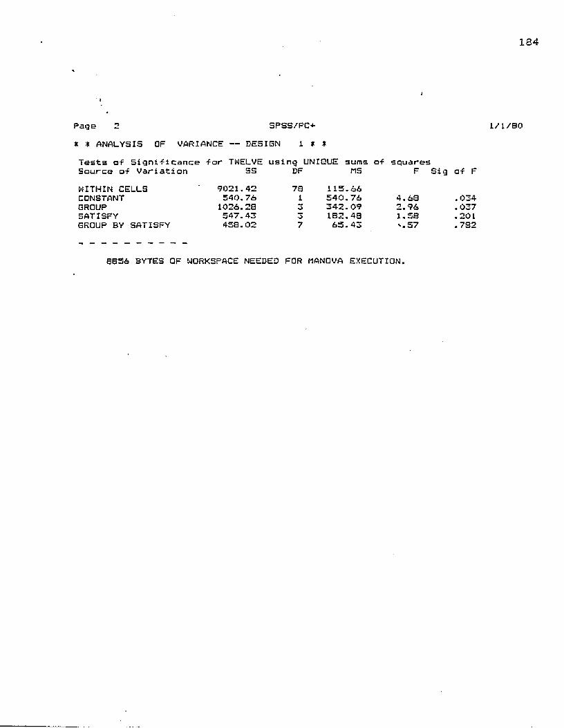
134

Page 2 SPSS/PC+* * ANALYSIS OF VARIANCE — DESIGN 1 * *Tests of Significance for TWELVE using UNIQUE sums of squaresSource of Variation SS DF NS F Sig of FWITHIN CELLS 9021.42 73 115.66CONSTANT 540.76 1 540.76 4.63 .034GROUP 1026.2S 3 342.09 2.96 .037SATISFY 547.43 3 132.43 1.58 .201GROUP BY SATISFY 453.02 7 65. '.57 .732

l/l/BO

8356 BYTES OF WORKSPACE NEEDED FOR NANOVA EXECUTION.

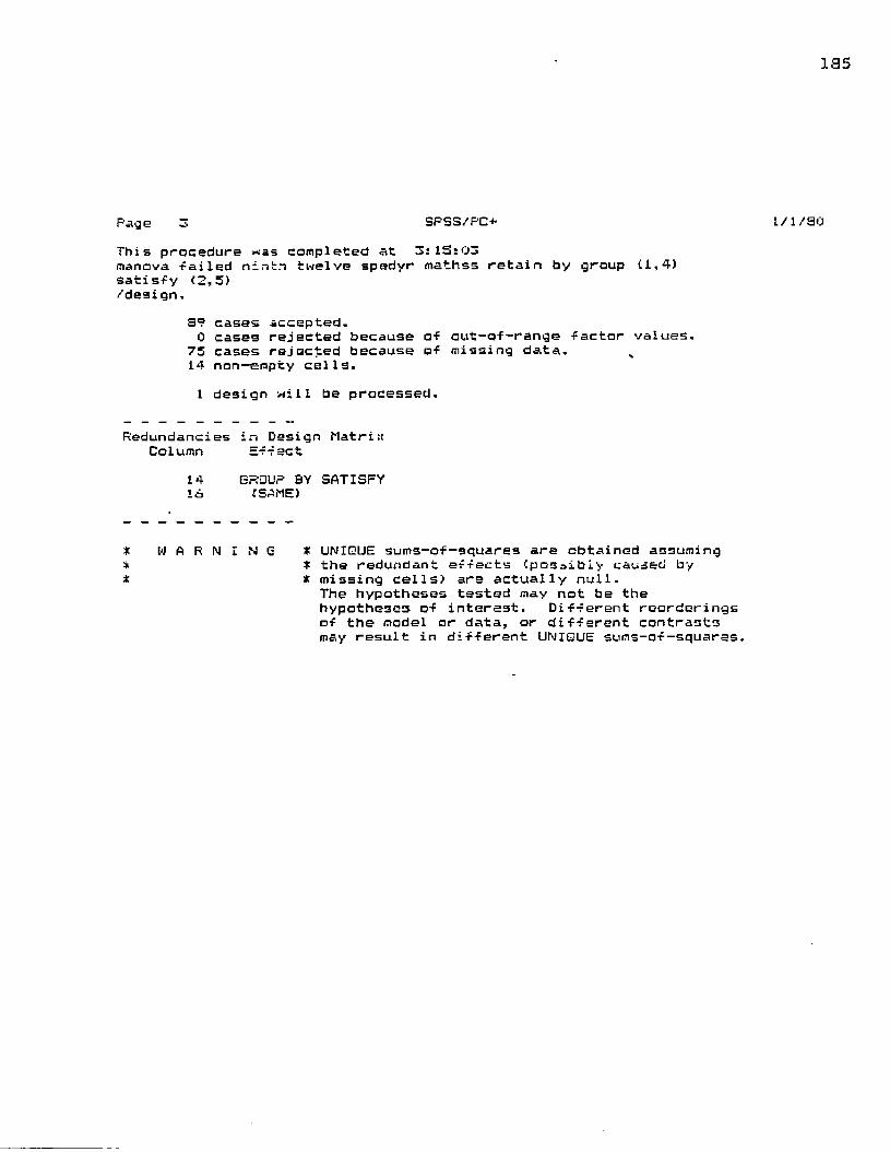
135

Paige 3 SPSS/PC-**This procedure «ias completed at 3:15:03manova -failed ninth twelve spedyr mathss retain by group (1,4) satisfy (2,5)/design,

S? cases accepted.0 cases rejected because of aut-of~range factor values.

75 cases rejected because of missing data. „14 non-empty cells.1 design will be processed.

Redundancies in Design Matrix Column Effect

14 GRDUP BY SATISFY 16 (SAME)

* W A R N I N G * UNIQUE sums-of-squares are obtained assuming* * the redundant effects (possibly caused by* * missing cells) are actually null.

The hypotheses tested may not be the hypotheses of interest. Different reorderings of the model or data, or different contrasts may result in different UNIQUE sums-of—squares.

1/1/30

186

. v gt d and totalst It 4) satisfy=l.variabis labels satisfy 'student satisfaction with school', value labels satisfy 1 'high dissatisfy' 2 'almost dissatisfy’3 'mod satisfy’ 4 ’almost satisfy' S ’high satisfy', recode sew (1 = 1 ) (2 = 0 )/momoc dadoc (01=0) (11 thru 15=0) (0 0 = 1 ) (02 thru 10=1).value labels se:; 0 'female’ 1 ’male’/momoc dadoc 0 ’not working' 1 ’working’.recode gpa (0.00 thru 1.00=1) (1.01 thru 2.00=2) (2.01 thru 3.00=3 /(3.01 thru 4.00=4).value labels gpa 1 ’well below’ 2 ’below’ 3 ’avg! 4 'above avg’. manova twelve by group (1,4) gpa (1,4)The raw data or transformation pass is proceeding

164 cases are written to the uncompressed active file./print=cell info(means)/design.

164 cases accepted. "O cases rejected because of out-of—range factor values.0 cases rejected because of missing data.

15 non-empty cells.1 design will be processed.

Cell Means and Standard DeviationsVariable .. TWELVE twelfth grade absenteeism rate

FACTOR CODE Mean Std. Dev. NGROUP female aGPA bel aw 9.233 5.615 ■JGPA ' avg 6.622 *_>, ijQo " **•GPA above av 5. 689 2.418

GROUP male attGPA wel 1 bel 38.500 27.541 ■I)GPA below 9. 633 4. 125 9GPA avg 7. 927 4. 172 Z-sGPA above av 5. 056 2.395 9

GROUP female nGPA well bel 20.400 . ooo 1GPA bel ow 21.184 13.744 *9GPA avg 16.550 5.260 *GPA above av 13.600 2.884 •j

GROUP male nonGPA well bel 42.582 20.087 : lGPA bel ow 18.104 9. 214 35GPA avg 13.900 7. 425 3GPA above av 13.150 4. 455

Far entire sample 14.754 13.294 • _ 1

Reduncancies in Design Matr;:: Column Effect

16 GROUP BY GPA

•* W A R N I N G * UNIQUE sums-of—squares are obtained assuming:* S the redundant effects (possibly caused byt missing cells) are actually null.

The hypotheses tsstsd may not be the hypotheses of interest. Different reorder i c s of the model or data, or different contrasts may result in different UNIQUE sums—af-squarss.

Page 9 SPSS/PC+ 1/1/80* * ANALYSIS OF VARIANCE — DESIGN 1 * *Tests of Significance -for TWELVE using UNICUE sums of squaresSource of Variation SS DF MS FWITHIN CELLS 12797.07 149 85. 89CONSTANT 1535.31 1 1335.31 15. 55GROUP 1124.07 3 374. 69 4.36GPA 545.81 3 114.60 1 • 33GROUP BY GPA 658.23 8 82. 23 . 96

of F

.000

. 008

.265

. 471

0856 BYTES OF WORKSPACE NEEDED FOR MANOVA EXECUTION.

188

Page a SPSS/PC+ 1/I/BOThis procedure was completed at 3:19:17recode gpa CO.00 thru 1.00=1) Cl.01 thru 2.00=2) C2.0I thru 3.00=3)C3.01 thru 4.00=4).value labels gpa 1 ’well below’ 2 ’below' 3 ’avg’ 4 aoove avg’. manova twelve by group (1,4) gpa (1,4).The raw data or transformation pass is proceeding

164 cases are written to the uncompressed active file.

NOTE 12167The last subcommand is not a design specification— A ftul 1 factorial model is generated for this problem.

164 cases accepted.0 cases rejected because of out-of—range factor values.0 cases rejected because of missing data.

15 non-empty cells.1 design will be processed.

Redundancies in Design Matri:: Column Effect

16 GROUP BY GPA

* W A R N I N G * UNIQUE sums—of— squares are obtained assuming* * the redundant effects (possibly caused by* t missing cells) are actually null.

The hypotheses tested may not be the hypotheses of interest. Different reorderings of the model or data, or different contrasts may result in different UNIQUE sums-of-squares.

APPENDIX H NINTH GRADE STUDENT DATA

189

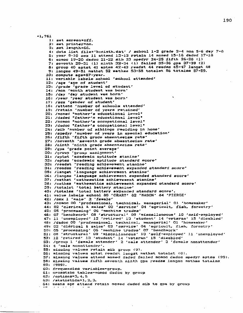
190

*1,7611 : set aoroen=off.2 : set printerBon.3: set length»6 6 .4: data list file"*b:ninth. d a t ' / school 1-2 grade 3-4 men 5-6 day 7-8 5: year 9-10 sex 11 attend 12-13 retain 14 momed 15-16 daded 17-18 6 : momoc 19-20 dedoc 21-22 sib 23 spedyr 24-25 fifth 26-28 (1)7: seventh 29-31 <1) ninth 32-34 (1) failed 35-36 gpa 37-39 (2)6 ; group 40 aptst 41 eptea 42-43 raadst 44 readss 45—47 langst 489s langss 49—51 reathst 52 nethaa 53-55 totalst 56 totalss 57-59.

10: compute age*87-year.1 1 : variable labels school 'school attended*1 2 : /age 'age of student*13: /grade 'grade level of student'14: /mon 'month student van born'15: /day 'day student was horn'16: /year 'year student was born' '17: /sex 'gender of student'18: /attend 'number of schools attended'19: /retain 'number of years retained'2 0 : /momed "mother's educational level*2 1 : /daded "father's educational level*2 2 : /momoc "mother's occupational level*23: /dadoc "father's occupational level"24: /sib 'number of siblings residing in home'25: /spedyr 'number of years in special education'26: /fifth 'fifth grade absenteeism rate'27: /seventh 'seventh grade absenteeism rate'28: /ninth 'ninth grade absenteeism rate'29: /gpa 'grade point average'30: /group 'group assignment'31: /aptst 'academic aptitude stanine'32: /aptss 'academic aptitude standard score'33: /readat 'reading achievement stanine'34: /readss 'reading achievement expanded standard score'35: /langst 'language achievement stanine'36: /langss 'language achievement expanded standard score'37: /mathst 'mathematics achievement stanine'38: /mathss 'mathematics achievement expended standard score'39: /totalst 'total battery stanine'40: /totalas 'total battery expanded standard score'.41: value labels school 80 'C2ARY* 82 'MASON' 84 'PIERCE'42: /sex 1 'male' 2 'female'43: /momoc 00 'professional, technical, managerial' 01 'homemaker'44: 02 'clerical £ sales' 03 'service' 04 'agricult, fish, forestry'45: 05 'processing' 06 'machine trades'46: 07 'henchwork' 08 'structural' 09 'miscellaneous' 10 'self-employed' 47: 11 'unemployed' 12 'retired' 13 'student' 14 'veteran' 15 'disabled'48: /dadoc 00 'professional, technical, managerial' Ol 'homemaker'49: 02 'clerical £ sales' 03 'service' 04 'agricult, fish, forestry'50: 05 'processing' 06 'machine trades' 07 'benchvork'51: 08 'structural' 09 'miscellaneous' 10 'self-employed’ 11 'unemployed' 52: 12 'retired' 13 'student' 14 'veteran' 15 'disabled'53: /group 1 'female attender* 2 'male attender' 3 'female nonattender'54: 4 'male nonattender'.55: missing values retain sib group (9).56: missing values aptst readst langst mathst totalst <Q>.57: missing values attend momed daded failed momoc dadoc spedyr aptss <99).58: missing values fifth seventh ninth gpa readss langss mathss totalss59: (999).60: frequencies varlables«group.61: crasatabs tables=*momoc dadoc by group 62: /aptions=»3,4,5 63: /statisticsal, 2, 3.64: means age attend retain momed daded alb to gpa by group

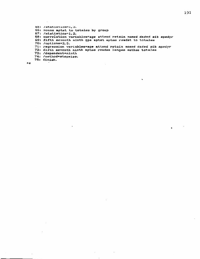
191

o o : /statistics':!,GG: means aptst. to totalss by group 67: /statistics 3 I,2.6 8 : correlation variablessage attend retain momed daded sib spedyr 69: fifth seventh ninth gpa aptst aptss readst to totalss 70: /options»3,5.71; regression variables"age attend retain momed daded sib spedyr 72: fifth seventh ninth aptss readss langss mathss totalss 73: /dependent=ninth 74: /method"stepwise.75: finish.

192

8 >sdlin ninth.dat End of input file *-1 . 1661

11 *820905037210401£1201071020060310630515023413692469047103637 2: 8409031372204009110107100108087327042083 4717 57273; 8009111171105112 OS 0OOO4S SI30609243393697367337053632 4: B4091SOI712040131600103060130220210320015s 80030315722030121209 1 06705504601175144337075706572247126 : 8403122271206112120206400153S06507S000836557: 8409042472107014120111SO005310847£140504 36342611S678265S8 : 32090805721030161401022000010010030039223689839373437599737 9: 340307087220401S1601001000580430320035816543829674287473773 lOs 80090619711080121001061040630992271612542372570468226873680 11: 80090305712 012120112100 10814703113312: 80030226722040161201021000580940440036714467732775167337753 13: 8009112171103213101307000050056112171002127 4685363414s 82030103722030 0202100064065079002751447574857195726573115: 800907167210301112010310005619523627058444436883655 16: 8203032271106112120103300047 103032172 368836652688368017: 800910017110631212010300009418373021000418: 84091110722050 120303100 108041001236472447004714471319: 80090102712071121003 2000831031810710831272638463047063675£0: 80030116711061111203000001112304023101746537787366026884712 21: 8409110472209011 Ol 004067132244051083 22: Q0091204712 00 10429324000323: 8009051672104012140108306047047029012922 47224700£4: 80090711721060121201021001281201430608327626777571657245739 25: Q409010973104012160200300022 043002832653981767427742776726: 840909197211001218010010122522050014033427: 82091115722040 00 200022 245150923 574946875718471928: 8409051471107012 01 100064 '3551304243333b7545354?10366029: 82090717722030121201023001421493071108334465742571547175725 30: 8409061572105012120102100092058249120674 472515962680266731: 8409013172103014140106100042058052002332 677767275721674232: 80090712722 00 03935318010333: 80090720721030121201082000780290890028324466774672887476750 34: 82091001722090101007072000470512060420036536767774797807765 35: 8009011772110110 03 1000892641070224224463695367436: 82090326721040091201070000970670870122524465741470357205721 37: 82090628711061131200072100171433361603043423676468267303696 38: 3009021572203012090711200075077140032003548 7747572239: 82090325722030121202002000080490790026716576767775557246749 40: 8009032072210012120707100 2110712535513740570741: 820904217220501212 03003043045052331235370536723690368942: 82090908721050171200071000080050350021725506767775867286751 43: 80091201722 010110307100022012028003331551675977515724674544: 80090830721030161601001000140591020220024456754571547175732 45: 84091026722030 01OOl00000073037003001444575357144714572746: 8409012771207210100707100010427274260503 2622369447: 82090806712061 010040001100403309167148: 82090410731 OO 074078003582971962698169781980049: 800909217220601316070350010614315101258350: 84090424711042121101071000751753762701745484716470047174711 51: 8409071172106016140002000 18303158452: 84090628711031 205058157148071831340471146904712470453: 80091223711040121201075000531320640228327626777672987516752 54: 8009121271104012140200100028 01800275255: 8409052172208010 07 400011063275021253234471257205724471956: 8003042571208012110114200069 07500250157: 84030405721030121202072000781171941206745495740470147134718 58: 80090610722030121201071000530080260038317603804877477368771 59: 840902067210301212020210009706204200233254957505719672S5732 60: 84090616722 OO 14317903158361: 8209072271104112130107207033123250071004 62: 84090210722100111101 200047087157070643

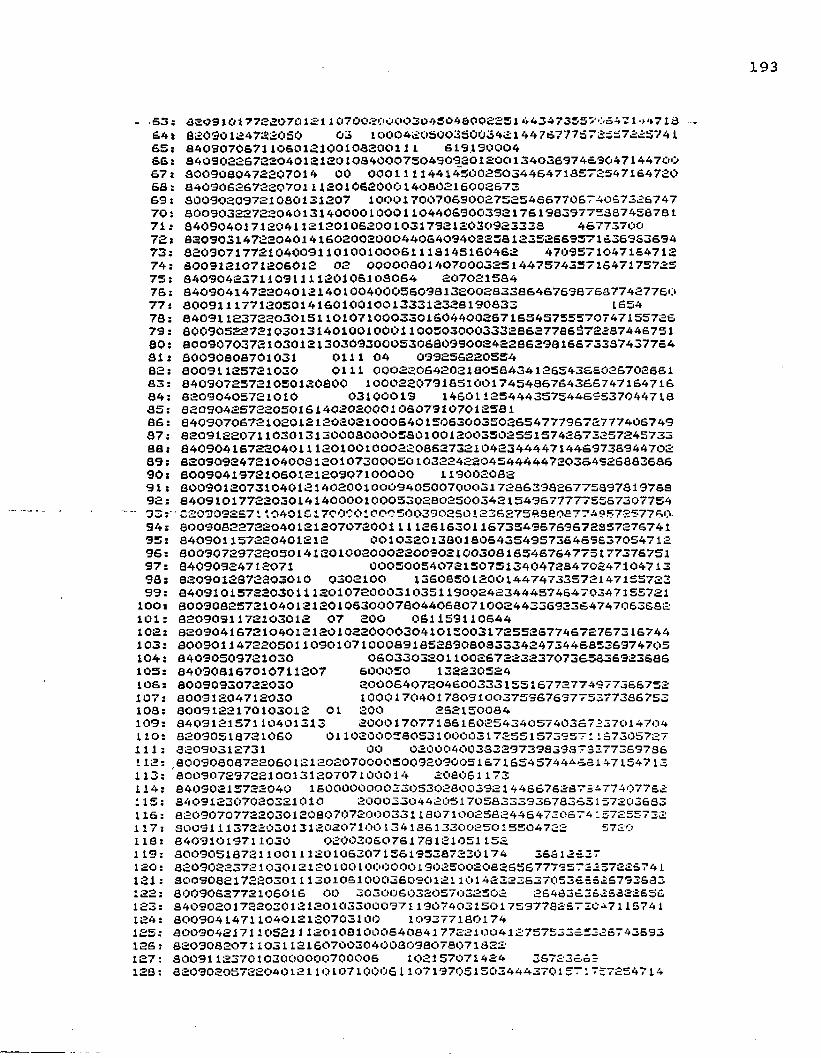
- 53; 82091017722070121 1 0700800003043048002251 44347355705471 ->‘>718£4! 82090124722050 03 1000420500330034214476777S7255722S74155: 34030706711060IS100106300111 61913000466! 84090226722040121201084000750490920120013403697463047144700 67s 6009060472207014 00 000111144145002503446471857254716472066: 640906267220701112010620001406021600267369: 30090209721060131207 100017007069002752546677067406732674770: 60090322722040131400001OOO110440690033217619839775667456761 71 i 3409040171204112120106200103179212030923323 4S77370072: 6209031472204014160200200044064094022531235266957163696369473; 3209071772104009110100100061113145160462 470957104716471274; 3009121071206012 02 000008014070003251447574357134717572575: 8409042371109111120105103064 20702153476: 34090414722040121401004000560981320028336646769876377427760 77; 3009111771205014160100100133312328190333 165478: 840911237220301S1101071000330160440026716545755570747155726 79: 80090522721030131401001000110050300033328627786372237446751 80: 8009070372103012I303093000530630990024228629816673337437764 81: 30090808701031 0111 04 09925622055482: 80091125721030 0111 00022064202180584341265436602670266183: 84090725721050120800 100022079185100174548675436574716471684: 62090405721010 03100019 14601125444357544SS53704471885: 820904257220501614020200010607910701£58186: 84090706721020121202021000540150630035026547779672777406749 37; 82091220711030131300080000580100120035025515742672257245733 88: 84090416722040111201001000220862732104234444714469736944702 89: 82090924721040031201073000501032242204544444720364326883686 90: 8009041972106012120907100000 1190020829 1 s 80090120731040121402001000940500700031728639826775897819786 92: 84091017722030141400001000530280250034215496777775567307754

- 93;“ 62030926711040161700001000500390250123627583808774957257760. 94: 80090822722040121207072001111261630116735496769672357276741 95: 840901157220401212 00103201380180643549573646983705471296 : 80090729722050141201002000220090210030816546764773177376751 97: 84090924712071 00050054072150751340472347024710471398s 8209012872203010 0302100 136085012001447473357214715572399: 84031015722030111201072000310351190024234445746470347155721 lOO: 80090825721040121201063000780440680710024433692364747063682 101: 8209091172103012 07 200 061153110644102: 82090416721040121201022000030410150031725526774572767316744 103: 80090114722050110901071000891852890803333424734468536974705 104: 84090509721030 060330320110026722323707363636923686105: 340908167010711207 600050 132230524106: 80090930722030 2000640720460033315516772774377366752107: 80091204712030 1000170401730910037596769775377386753108: 8009122170103012 01 200 252150084109: 840912157110401313 2000170771861602543405740367237014704HO : 82090518721060 0110200058053100003172551573257 : 1S7305727111: 32090312731 OO 0200040038329739839373377369736112: ,80090808722060121£0207000050092090051£716545744468147154713 113:'8009072972210013120707100014 208051173114: 84090215722040 16000000003305302800392144667S2S7 = 4774r;i77£l:.115: 340912307020321010 2000330442051705833393678365157203633116: 82090707722030120807072000331180710025824464720674 157255732 117: 30091113722030131202071 OO 13 41861330025015504722 5720118: 84091019711030 0200306076178121051152119: 8009051872110011120106307156195387220174 36612637120: 82090223721030121201001000000190250020826567779572257226741121: 3009082172203011130106100036090121101423236370536 =625793683 122: 8009062772106016 OO 303006032057032502 2648363525822656123: 840902017220301212010330009711907403150175977826730^7116741124: 8009041471104012120703100 109377180174125: 80090421711052111201081000640841772210041275753365326743593126: 820908207110311£160700304008098078071822127: 8009112370103000000700006 102157071424 36723653128: 82090205722040121101071000611071970515034443701571737254714

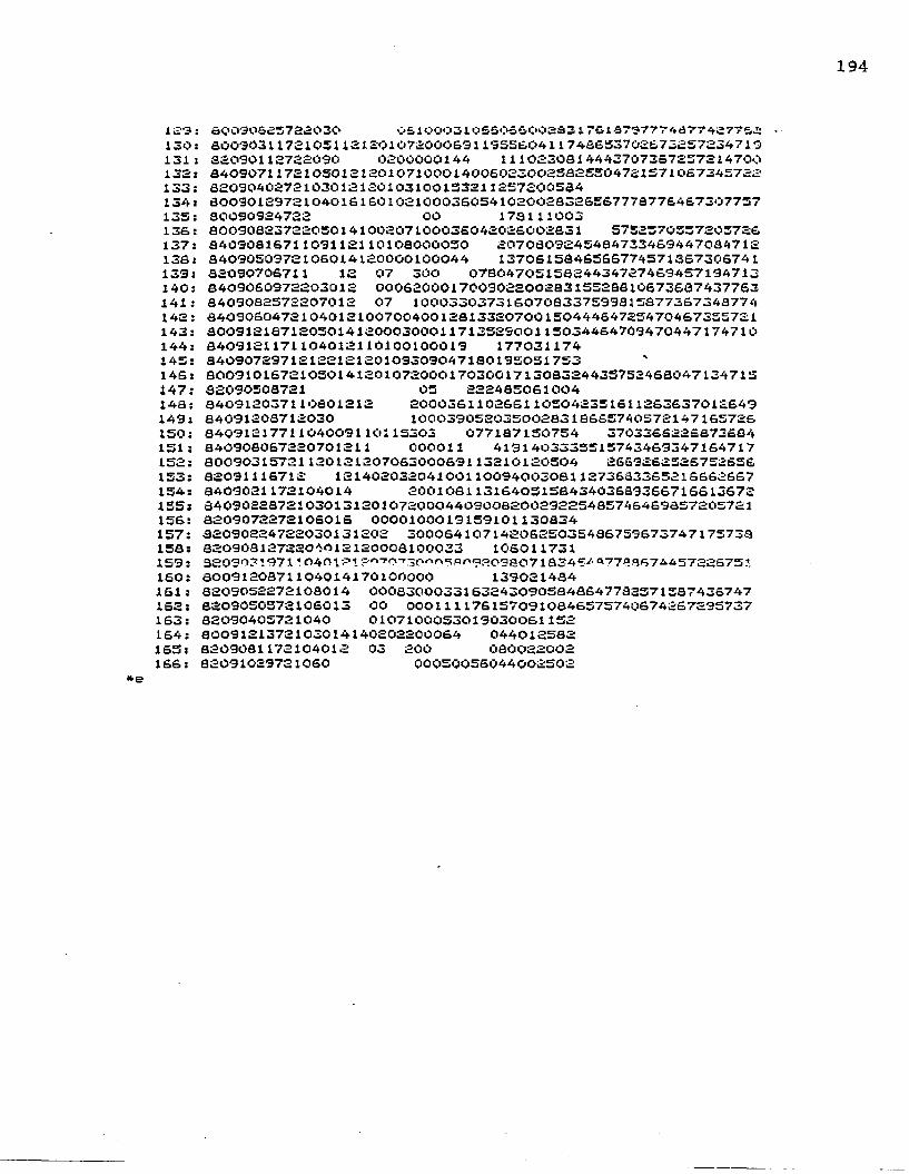
194

123: 30090623722030 OS 100031 OSSOSCOOSSSl 701S7377T^d7r4a7?&£130: 3003031172103112ISO1072000£31195S60411746653702673257234710 131: £2090112722030 0200000144 1110230814443707357257214700132: 34090711721OSO121201071OOO140060230023325304721571067345722 133: 3209040272103012120103100153211257200584134: 30090129721040161601021000360541020023326567773776467307757 135: 30090924722 00 173111003136: 3009032372205014100207100036042026002331 5752370557205726137: 34090S1671109112110103000050 2070309245434723469447034712133: 3409050972106014120000100044 1370615346566774571367306741139: 32090706711 12 07 300 0730470515324434727469457194713140: 8409060972203012 00062000170090220023315523310673637437763141: 3409032572207012 07 1000330373160703337599315377367343774142: 34090604721040121007004001231332070015044464725470467355721 143: 30091218712050141200030001171352900115034464709470447174710 144, 6409121171104012110100100019 177031174145: 3409072971212212120109309047130195031753146: 80091016721050141201072000170300171303324433752463047134715 147: 32090503721 05 222485061004148; 840912037110301212 200036110266110504235 1611263637012649149: 34091203712030 1000390520350023318665740S72I47165726ISO: 8409121771104009110115303 077187150754 3703366226373664151: 840903067220701211 000011 4191403335515743469347164717152: 8009031572112012120706300069113210120504 266926252S752656153: 82091116712 121402032041001100940030811273633365216662667154: 8409021172104014 200103113164O515B434036393S6716613672155: 34090223721030131201072000440900320029225485746469357205721 156: 8209072272106016 0000100019159101130334157: 32090224722030131202 3000641071420625035436759673747175733158; 820908127220 4012120003100033 106011731159: 3209031971 1 0401 PI 8345^' Q776367445722S75.11,160: 8009120871104014170100000 139021484161: 3209052272108014 00083000331632430905848647732571587436747162: 8209050572106013 00 0001111761570910846575740674267295737163: 82090405721040 0107100053019030061152164: 8009121372103014140202200064 044012582165: 8209081172104012 03 200 080022002166: 32091029721060 00050055044002502

APPENDIX IONE-WAY ANALYSIS OF VARIANCE SUMMARY TABLES FOR NINTH GRADE DATA

195

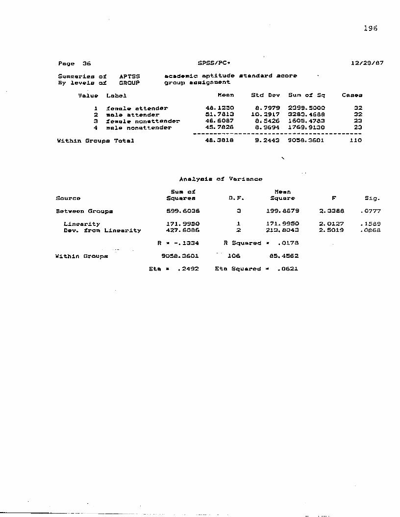
196

Page 36 SPSS/PC* 12/29/87Summaries of APTSSBy levels of CROUP

academic aptitude standard score group assignment

Value Label Mean Std Dev Sum of Sq Cases1 female attender 48.1250 8 .7979 2399.5000 322 male attender 51.7813 10.2917 3283.4688 323 female nonattender 46.6087 8.5426 1605.4783 234 male nonattender 45.7826 8 . 9694 1769.9130 23

n Groups Total 48.3613 9.2443 9058.3601 H O

Analysis of Variance

SourceBetween Groups

LinearityDev. iron Linearity

Within Groups

Sum of Squares599.6036171.9950 427. 6086

R « 1334905a.3601

Eta » .2492

MeanD, F. Square

12

199.8679171.9950 213.8043

R Squared » .0173106 35.4562

Eta Squared * .0621

F2 . 33832. 0127 2. 5019

Sig. . 0777 . 1539. oeea

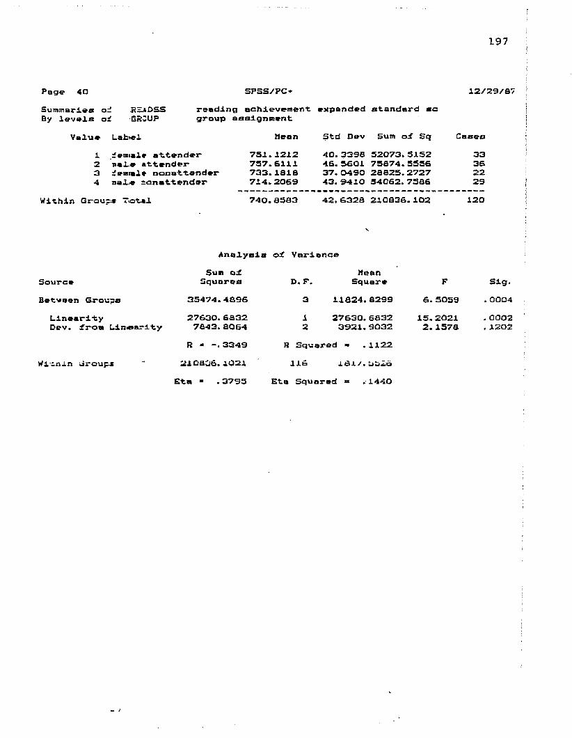
197

Page 40 s p s s /p c * 12/29/87Summaries oi By levels oi

JtZiDSS reading achievement expanded standard sc■GR3UP group assignment

Value Lafctel Mean Std Dev Sum of Sq Cases1 femtal* attender 751.1212 40. 3398 52073. 3152 332 «al« attender 757.6111 46. 5601 75874. 5536 363 female nonattender 733.iaie 37. 0490 28623. 2727 224 sale conattender 714.2069 43. 9410 54062.7586 29

Within Group* Tctil 740.8583 42. 6328 210836.102 120

Analysis of Variance

SourceBetween Groups

Linearity Dev. from Lini

Wicnin Jroupi

Sum of Squares

35474.489627630. 6832

■earity 7843.8064R - 3349

210836.1021Eta - .3793

MeanD.P. Square

3 11824.82991 27630.68322 3921.9032

R Squared ** .1122116 161/.

Eta Squared » -■ 1440

F6.5059

15. 2021 2. 1578

Slg.. 0004, 0002 . 1202

198

Page 44 SPSS/PC* 12/29/67Summaries of By levels of

LANGSS language achievement expanded standard aGROUP group assignment

Value Label Mean Std Dev Sum of Sq Cases1 female attender 721.6430 31.2659 30304.2iaa 322 male attender 719.0270 36.4063 53106.9730 373 female nonattender 706.2500 36.3261 30350.5000 244 male nonattender 675.3793 36.4510 37202.6276 29

Within Groups Total 707.2705 35.7661 150964.519 122

Analysis of Variance

SourceBetveen Groups

LinearityDev. Iran Linearity

Within Groups

Sum of Squares

41427.554334689.0077 6736.5460

R * -.4246150964. 5193

Eta - .4640

D. F.312

MeanSquare

13609.184634669.0077 3369.2734

R Squared “ .1803lia 1279.3603

Eta Squared M . 2153

F10.793627.1143 2.6336

Sig.. oooo. OOOO . 0760

199

Page 48 SPSS/PC* 12/29/87Summaries of By levels of

MATHSS mathematics achievement expanded standarGROUP group assignment

Value Label Mean Std Dev Sum of Sq Cases1 female attender 720. 8182 16.5576 8772.9091 332 male attender 727. 28S7 21.8384 16215.1429 352 female nonattender 715.3800 23.3057 13035.7600 254 male nonattender 702.8846 22.5075 12664.6538 26

n Groups Total 717.6555 20.9945 50688.4658 119

Analysis of VarianceSum of Mean

Source Squares D.F. Square F Slg.Between Groups 9380.4082 3 3126. 8027 7.0940 . 0002

Linearity 5932. 8660 1 5932.8660 13.4603 . 0004Dev. from Linearity 3447.5421 2 1723. 7711 3. 9108 . 0227

R ■ -.3143 R Squared - .0988Within Groups 50686.4658 115 440.7693

Eta * . 3952 Eta Squared - .1562

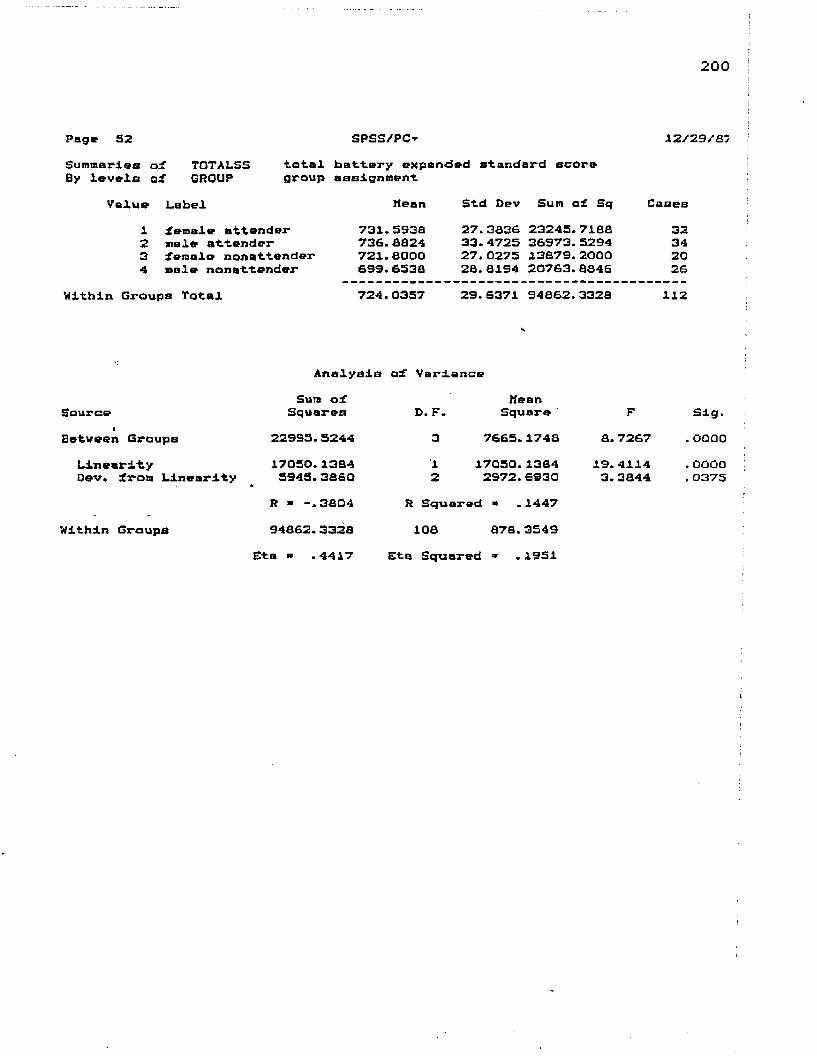
200

Page 52 SPSS/PC-* 12/29/a:Summaries of TOTALSS total battery expanded standard scoreBy levels of GROUP group assignment

Value Label Mean Std Dev Sum of Sq Cases1 female attender 731.5938 27.3836 23245.7188 322 male attender 736.8824 33.4725 36973.5294 343 female nonattender 721.8000 27.0275 13879.2000 204 male nonattender 699.6538 28.8194 20763.8846 26

Within Groups Total 724.0357 29. 6371 94862.3328 112

Analysis of Variance

SourceBetween Groups

LinearityDev. iron Linearity

Within Groups

Sure of Squares

22995. 524417050.1284 5945.3880

R - -.380494882. 3328

Eta - . 4417

D. F.312

Kean Square '

7685.174S17050.1384 2972.6S30

R Squared * .1447108 878.3549

Eta Squared =* . 1951

FS.7267

19.4114 3.3844

Slg.. OOOO. OOOO , 0375

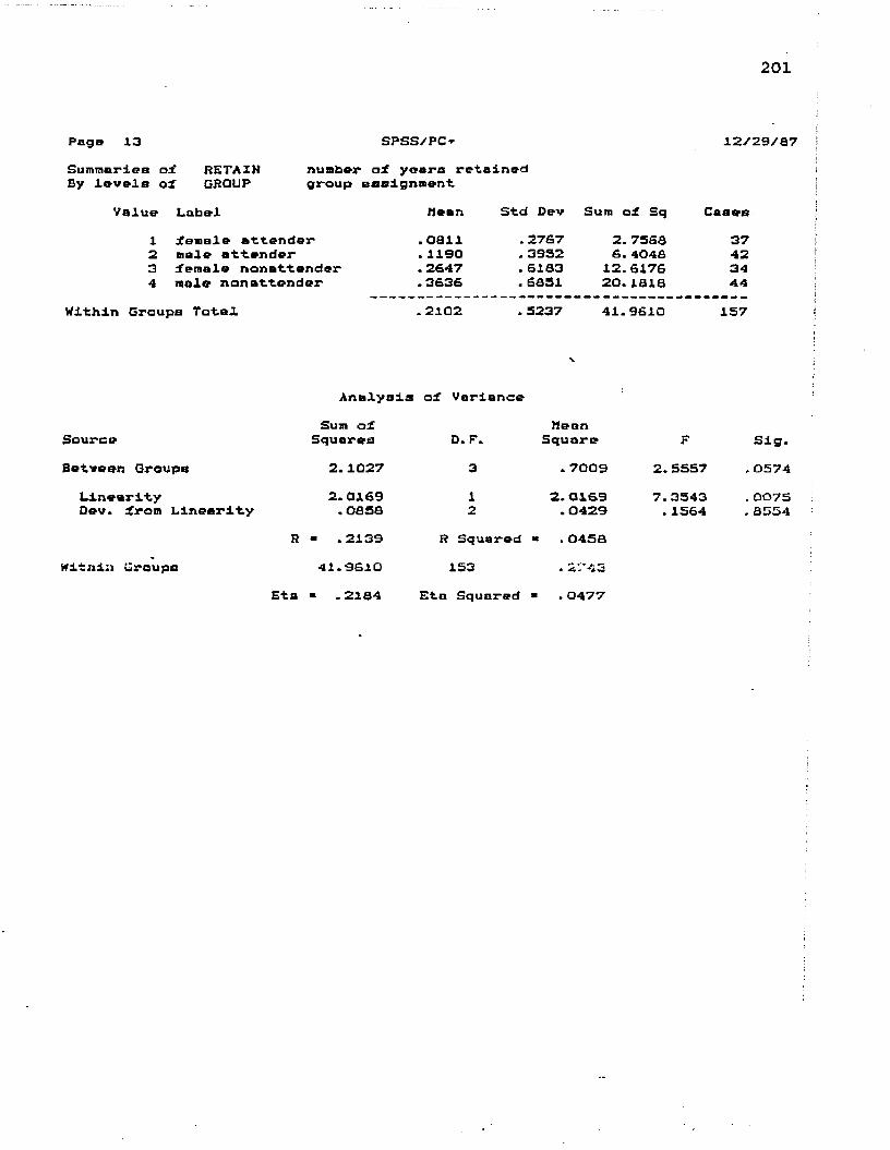
201

Page 13 SPSS/PC* 12/29/37Summaries oi RETAIN number o± years retainedBy levels of GROUP group assignment.

Value Label Mean Std Dev Sum ol Sq Cases1 Jemale attender2 male attender3 female nonattender4 male nonattender

.0011

.1190

. 2647

. 3636

2767 2. 7560 3952 6.4040 6103 12.6176 6051 20.1010

37423444

Within Groups Total .2102 5237 41.9610 157

Analysis of Variance

X.

SourceSum of

Squares D. F.Mean

Square F Slg.Between Groups 2.1027 3 .7009 2.5537 , 0574

LinearityDev. iron Linearity

2.0169. oasa

12

2.0169 7.3543 . 0429 . 1564

. 0075 , 0554

R ■ .2139 R Squared * .0450Witnin Groups -41.9610 153 . 2743

Eta - .2104 Eta Squared ■ .0477

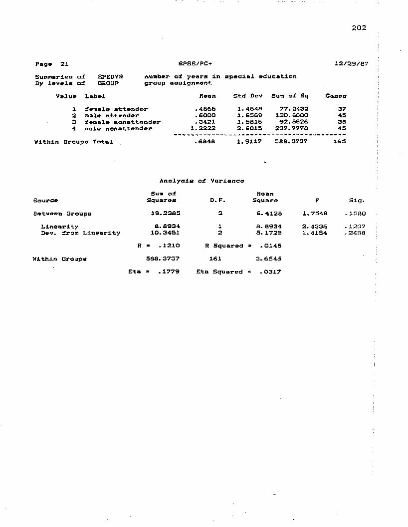
202

Page 21 SPSS/PC* 12/29/87Summaries of By levels of

SPEDYR number of years In special educationGROUP group assignment.

Value Label Mean Std Dev Sum of Sq Cases1 female attender . 4865 1.4648 77.2432 372 male attender .6000 1.6569 120.8000 453 female nonattender . 3421 1.5816 92.5526 384 male nonattender 1.2222 2.6015 297.7778 45

Within Groups Total .6848 1. 9117 588.3737 165

Analysis of Variance

SourceBetveen Groups

LinearityDev. from Linearity

Within Groups

Sum of Squares19.23858. 8934

10.3451R - .1210

588. 3737Eta - .1779

D. F.312

R Squared 161

Eta Squared

MeanSquare6. 41288. 8934 5. 1725

> .01463.6545

■ .0317

F1.75482.4336 1.4154

Slg.. 1580. 1207 - 2458

Page 11 SPSS/PC* 12/29/37i

Suntnarlco of ATTEND number of schools attendedBy levels oi GROUP group assignment

Value Label Keen Std Dev Sum of Sq Cases1 female attender 4.3333 1.5856 88.0000 362 male attender 4.1667 1.3447 97.6333 423 female nonattender 3*7576 2.5499 208.0606 334 male nonattender 5.3864 2.3149 230.4316 44

Within Groups Total 4.6903 2.0334 624.3258 155

Analysis of Variance

SourceSum of

Squares D. F.henn

Square F Sig.Betveen Groups 68.8097 3 22.9366 5. 5475 . 0012

LinearityDev. from Linearity

42.9638 23. 8459

12

42.9638 12.9230

10.3913 3.1256

. 0016

. 0468R « .2490 R Squared = .0620

Within Groups 624.323d 151 4.1346 ■ —

Eta « . 3151 Eta Squared ■ .0993

204

Page 9 SPSS/PC- 12/29/87Suanariaa of AGE age of studentBy l»v«ls of GROUP group a s s i g n n u t

Value Label been Std Dev Sum of Sq Casas1 ienale attender 13.2105 .4132 6.3158 382 mala attender 13.1111 . 5318 12.4444 453 female nonattender 15.3158 .5253 lO.2105 384 mala nonattender 15.6000 . 6537 18.8000 45

Within Groups Total 15.3133 . 5430 47.7708 166

Analysis of Variance Sum of Dean

Source Squares D.F. Square F Sig.Between Groups 5.5401 3 1.9800 6. 7147 . 0003

Linearity 4.2879 1 4.2879 14.5411 . 0002Dev. from Linearity 1.6522 2 .8261 2. 8015 . 0637

R - .2825 R Squared - .0798Within Groups 47.7708 162 . 2949

Eta - .3326 Eta Squared " .1106

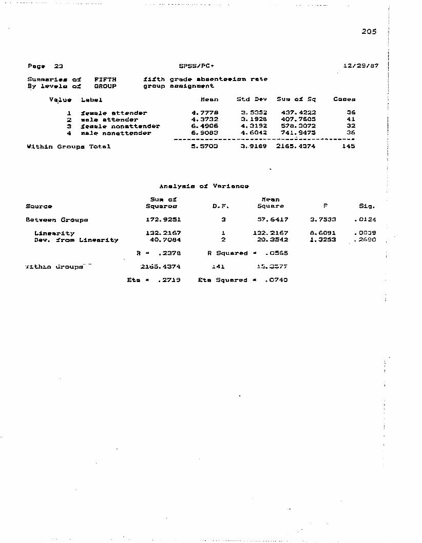
205

Page 23 SPSS/PC+ 12/29/87Summaries Of FIFTH fifth grade absenteeism rateBy levels of GROUP group assignment

Value Label Mean Std Dev Sura of Sq Cases1 female attender 4.7778 3.5352 437.4222 362 male attender 4.3732 3.1928 407.7605 413 female nonattender 6.4906 4.3192 578.3072 324 male nonattender 6.9083 4.6042 741.9475 36

Within Groups Total S. 5703 3.9189 2165.4374 145

Analysis of Variance

SourceBetween Groups

Linearity0«v. iron Linearity

tflthm Groups ”

Sum of Squares172. 9251132. 2167 40. 7064

R - .23732165.4374

Eta - .2719

D. F. 312

MeanSquare57. 6417

132. 2167 20. 3542

R Squared “ . 0565141 13.3577

Eta Squared ■ . 0740

F3.7533S.6091 1.3253

Sig.. 0124. 0039 . 2690

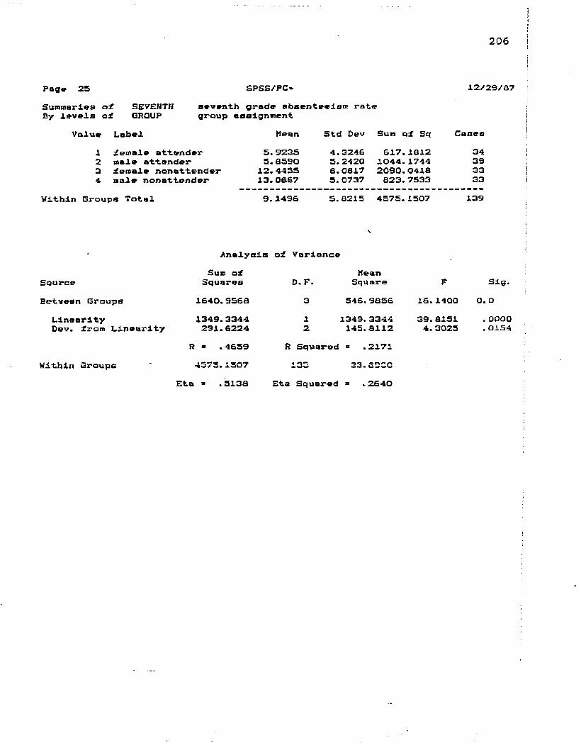
206

Pag* 25 SPSS/PC* 12/29/07Summaries of By levels of

SEVENTH seventh grade absenteeism rateGROUP group assignment

Value Label Hean Std Dev Sum of Sq Cases1 female attender 5.9235 4.3246 617.1812 342 male attender 5.8590 5. 2420 1044.1744 392 female nonattender 12.4455 8.0817 2090.0418 334 male nonattender 13.0887 5.0737 823.7533 33

Within Groups Total 9.1496 S.8215 457S.1507 139

Analysis of VarianceSum of Mean

Source Squares D. F. Square FBetveen Groups 1640.9568 3 546.9856 16.1400

Linearity 1349.3344 1 1349.3344 39.aisiDev. iron Linearity 291.6224 2 145.8112 4.302S

R - .4659 R Squared * .2171Within Groups 4575.1507 135 33.32CC

Eta * .5138 Eta Squared » .2640

Sig.O. O. OOOO . 0154

207

Page 27 SPSS/PC* 12729/87Summaries of HI NTHBy levels of GROUP

ninth grade absenteeism rate group assignment

Value Label Mean Std Dev Sum of Sq Cases1 female attender 6. 4318 3.3810 422.9621 382 male attender 6.2711 3.7878 631.2924 453 female nonattender 23.4447 8. 9289 2948.5139 384 male nonattender 26.6444 14.1323 8787.7511 45

Within Groups Total 15.7820 8.8858 12790. 5198 166

Analysis of Variance

SourceBetween Groups

LinearityDev. from Linearity

Within Groups

Sum of Squares

14933.791312758. 3989 2175. 3924

R - .878412790.5196

D. F.312

Mean Square '

4977.930412758.3989 1087.8982

Eta '.7339

R Squared * .4802J.S2 76. 9536

Eta Squared ■ .5387

F83.0488

161.5932 13.7784

Sig.. oooo, oooo . oooo

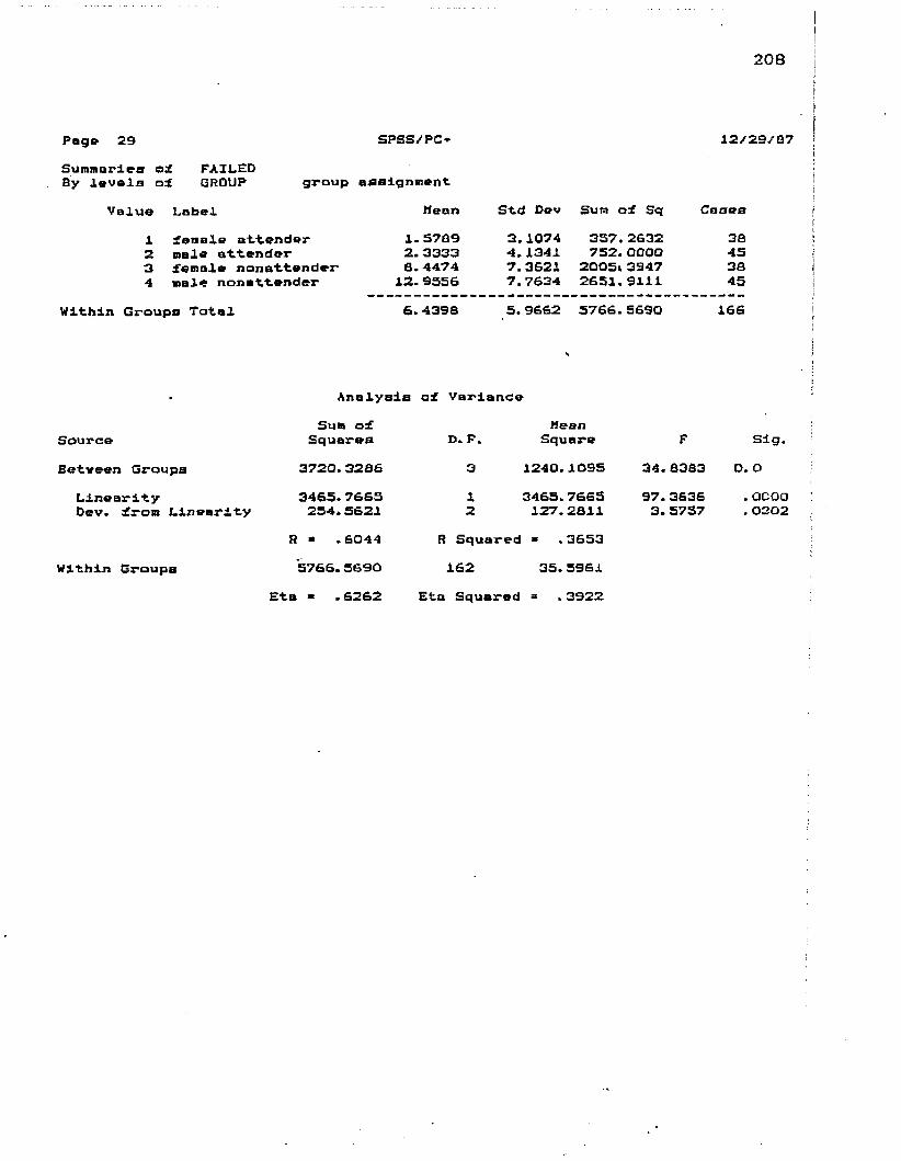
208

Page 29 SPSS/PC- 12/29/07Summaries of FAILEDBy levels of GROUP group asslgnment {

Value Label bean Std Dev Sum of Sq Cases r!1 female attender 1.5769 3.1074 337.2632 38 i2 male attender 2.3333 4.1341 752.OOOO 453 female nonattender 0.4474 7.3621 2005* 3947 3S i4 male nonattender 12.9556 7.7634 2651.9111 45 |

Within Groups Total 6.4398 5.9662 5766.5690 166 j

Analysis of VarianceSum of bean

Source Squares D. F. Square F Sig.Between Groups 3720.3286 3 1240.1095 34.8383 O. O

Linearity 3465.7663 1 3465.7663 97.3636 . OOOODev. from Linearity 254.5621 2 127. 2811 3. 5757 . 0202

R * .6044 R Squared - .3653Within Groups 5766.5690 162 35.5961

Eta » . 6262 Eta Squared ■ . 3922

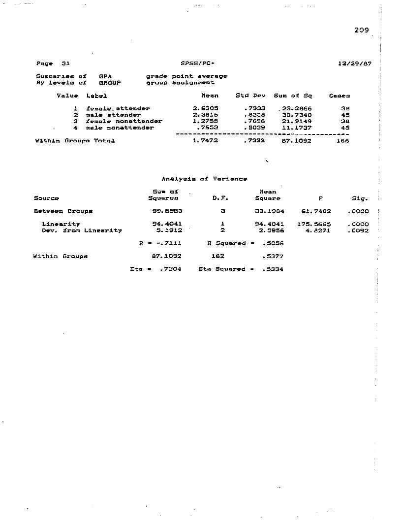
209

Page 31 SPSS/PC* 12/29/87Sumnarieo of GPA grade point, averageBy levels of GROUP group asslgnaent

Value Label dean Std Dev Sum of Sq Cases1 female.attender 2.6305 . 7933 .23.2866 382 male attender 2.3816 . 8358 30.7340 453 female nonattender 1.2755 . 7696 21.9149 384 male nonattender . 7653 . 5039 11.1737 45

Within Groups Total 1.7472 . 7333 87.1092 166

Analysis of Variance Sua of dean

Source Squares D. F. Square F Sig.Between Groups 99.5953 3 33.1984 61.7402 . OOOO

Linearity 94. 4041 1 94.4041 175.5665 . ooooDev. from Linearity 5.1912 2 2.5956 4.8271 . 0092

R » -.7111 R Squared > .5056Within Groups 87.1092 162 . 5377

Eta • .7304 Eta Squared . 5334

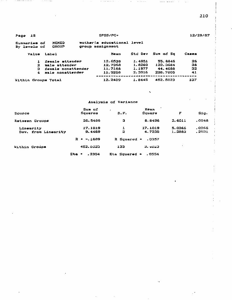
2 1 0

Page IS SPSS/PC+ 12/29/87Summaries of MOHED motherlE educational levelBy levels of GROUP group assignment

Value Label Mean Std Dev Sum of Sq Cases1 female attender 12.6538 1.4951 35.aS46 252 male attender 12.7368 1.8260 123. 3684 383 female nonattender ii.7ies 1.1977 44.4688 324 male nonattender 11.9268 2.3916 228.7805 41

Within Groups Total 12.2409 1.8445 4S2.5023 137

Analysis of Variance Sum of Mean

Source Squares D. F. Square F Sig.Between Groups 26.5488 3 8.8496 2.6011 .0548

Linearity 17.1019 1 17.1019 5.0266 . 0266Dev. from Linearity 9. 4469 2 4.7235 1.3883 . 2531

R - -.1889 R Squared - .0337Within Groups 452.5023 133 3.4023

Eta « .2354 Eta Squared - .0554

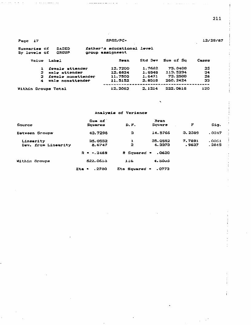
211

Pago 17 SPSS/PC* 12/29/87Summaries of DADEDBy levels of GROUP

father's educational levelgroup assignment

Value Label Mean Std Dev Sum of Sq Cases1 female attender 12.7200 1.7682 75.0400 252 male attender 12.8824 1.8548 113.3294 343 female nonattender 11.7500 1.6471 73.2500 284 male nonattender 11.3132 2.8518 260.2424 33

Within Groups Total 12.2083 2. 1214 322.0618 120

Analysis of Variance

SourceBetween Groups

LinearityDev. from Linearity

Within Groups

Sum of Squares43.729833.0352 8. 6747

R « -.2489522.0618

Eta » . 2780

D. F.312

R Squared 116

Eta Squared

MeanSquare14.376635.0552 4.3373

• .06204.5Quo

■ .0773

F3.23897.7891 . 9637

Sig.. 0247

. 0061

. 3845

212

Page 19 SPSS/PC* 12/29/67Summaries of SIBBy levels of GROUP

number of siblings residing in home group assignment

Value Label Mean Std Dev Sum of Sq Cases1 female attender 1.3869 .9936 34.5556 362 male attender 1.6829 1.0592 44.6760 412 female nonattender 1.7576 1.2508 50.0606 334 male nonattender 1. 5476 1.2533 64.4043 42

Within Croups Total 1.5921 1.1446 193.S990 152

Analysis of Variance

SourceBetween Groups

LinearityDev. from Linearity

Within Croups

Sum of Squares

2. B U S. 4216

2. 2900R - .0463

193.B990Eta » . 1196

D. F.312

R Squared 146

Eta Squared

MeanSquare

. 9372

. 4216 1.1950

> .00211*3101

> .0143

F.7153. 3218 9121

Sig.. 5443. 5714 . 4029

APPENDIX JCHI-SQUARE PROCEDURE FOR PARENTS * OCCUPATIONAL LEVELON NINTH GRADE DATA

213

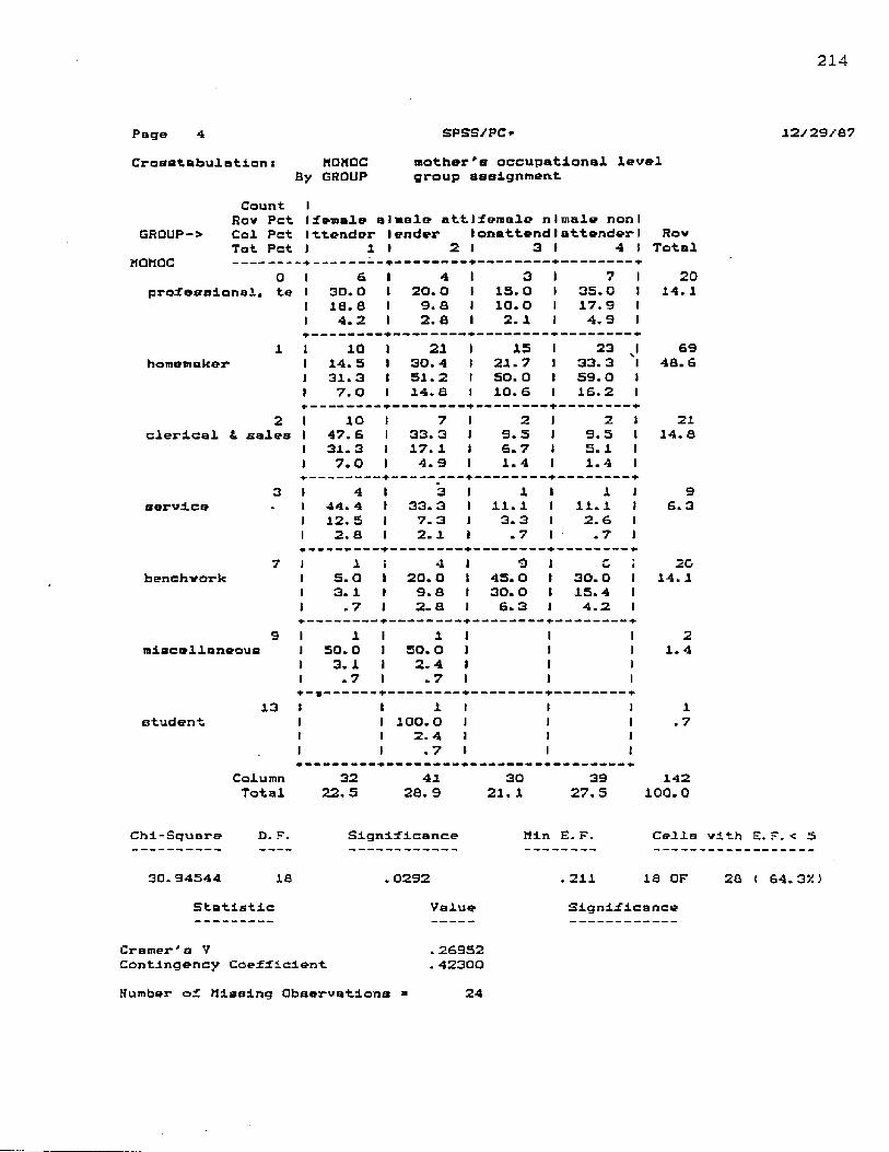
214

Page 4 SPSS/PC*- 12/29/87Crosatabulatiom MOMOC mother's occupational level

By GROUP group assignmentCount I

Raw Pet (female a)male attIfemale nI male non I GRQUP-> Col Pet Ittender lender lonattendIattenderI Rov

Tot Pet J I I 2 1 3 1 4 1 TotalOMQC -------

0 1 6 1 4 I 3 1 7 1 20professional, te 1 30. 0 1 2O.0 1 IS. O 1 35.0 1 14. 1

I is. a 1 9. a 1 10. o 1 17. 9 11 4.2 1 2. a 1 2. 1 1 4. 9 1

1 1 10 1 21 1 15 1 23 J 69homemaker 1 14. 5 1 30. 4 1 21.7 1 33. 3 1 48.6

1 31. 3 1 51. 2 1 SO. 0 1 59.0 11 7. O 1 14. a 1 10. 6 1 16. 2 1♦ ■

2 1 io 1 7 I 2 J 2 1 21clerical L sales 1 47. 6 1 33. 3 1 9. 5 1 9. 5 1 14. 8

1 31. 3 1 17. 1 1 5.7 1 5.1 JJ 7. 0 1 4. 9 1 1.4 1 1. 4 1-

3 1 4 1 3 1 1 1 1 J 9service 1 44. 4 I 33. 3 1 11. 1 1 11. 1 1 6. 3

1 12. 5 1 7. 3 1 3. 3 1 2. 6 11 2. a 1 2. 1 1 . 7 1 .7 1. -

7 1 1 i 4 1 9 1 U 1 2Gbenchwork 1 5. O 1 20.0 1 45. O 1 30. 0 1 14. 1

1 3. 1 1 9. a 1 30. 0 1 15. 4 11 . 7 J 2. a 1 6. 3 1 4.2 1—

9 1 1 1 i 1 1 1 2miscellaneous 1 50.0 1 50. O 1 1 1 1. 4

1 3. 1 1 2.4 1 1 11 .7 1 .7 1 1 1+ —* — — ----

13 1 1 1 1 1 1 1student 1 1 100. o 1 1 1 . 7

1 1 2. 4 1 1 11 1 . 7 1 1 1♦ —

Column 32 41 30 39 142Total 22.5 28. 9 21. 1 27. 5 100.0

Chi-Square D. F. Significance Min E.F. Celia vlth E.F. < 5

30.94544 18 .0292 .211 IS OF 28 < 64.3X)Statistic Value Significance

Cramer's V .26952Contingency Coefficient .42300Humber of Missing Observations ** 24

215

Page S SPSS/PC* 12/29/87Cronotobulation: DADOC fothar'e occupational level

By CROUP group assignment.- - - - Page 1 of 2

CountRoe Pet 1 female a 1 male attlfemale nlmale non 1

GRQUP-> Col Pet (ttender 1ender Ionnttend1attender1 RowTot Pet J i 1 2 1 3 1 4 1 Total

DADCIC ---0 t ii 1 io J 3 1 8 1 32

professional , t» 1 34. 4 1 31. 3 1 9. 4 J 25.0 1 26.21 38.7 1 27. a 1 13. 6 I 23.5 I1 9. 0 1 a. 2 1 2. 5 1 6. 6 1♦

2 1 4 1 7 I 1 1 2 1 14clerical 1 sales 1 28. 6 1 50.0 1 7. 1 1 14.3 1 11. 5

1 13.3 1 19.4 1 4.5 1 5.9 1) 3. 3 1 5. 7 1 .8 t 1.6 I

3 1 2 1 1 1 2 1 4 1 9service ) 22. 2 1 11. 1 1 22. 2 t 44. 4 1 7. 4

I 6.7 1 2.8 t 9. 1 1 11. 8 11 1.6 I .8 1 1.6 1 3.3 1

6 f 2 1 2 1 4 1 4 t 12machine trades 1 16. 7 1 16. 7 1 33. 3 1 33. 3 1 9.8

1 6. 7 1 5. 6 1 18. 2 1 1 1 . a 11 1. 6 1 1.6 I 3.3 1 3. 3 1. ■

7 1 6 1 11 ) 9 I 7 1 33benehvork 1 18.2 1 33. 3 i 27. 3 1 21. 2 f 27. 0

1 20.0 1 30. 6 1 40.9 1 20. 8 11 4. 9 1 9. 0 ) 7. 4 1 5.7 1♦ -

e i 2 1 3 j 1 4 1 9structural i 22. 2 1 33. 3 i 1 44. 4 1 7. 4

i 6. 7 1 a. 3 i 1 11.8 1i 1.6 t 2.5 1 > 3. 3 1* -

9 1 1 1 1 t 1 t 1 t 4miscellaneous 1 25. 0 1 25. O I 25. 0 1 25.0 1 3.3

1 3. 3 1 2. 8 ) 4. 5 1 2.9 1) . a 1 . a i . a ( .8 1

• +* oH l 1 1 I 1 1 2

self-employed i 50. 0 1 50. 0 1 t 1 1.8t 3. 3 1 2 . a I 1 1

- i . 8 I . a ) 1 1+ — ■*

ii t 1 I 1 1 3 1 4unemployed i 1 i 25. 0 1 75. Q I 3. 3

i 1 i 4. 5 1 a. a 1t 1 t . 8 1 2. 5 1-*■ — ♦

12 t 1 I 1 1 ! 1retired i 1 i iao. o 1 1 . a

i 1 I 4.5 1 1i I I . 8 1 t»—

Column 30 36 22 34 122(Continued) Total 24. 8 29. 5 18. 0 27. 9 lOO. o

216

Pag© 6 SPSS/PC*Croastabulatlon: DADOC father's occupotlonnl level

By GROUP group assignnent- - - - Pag©

Count IRov Pet 1 female a 1 male att female nlmole non 1

GR0UP-> Col Pet 1ttender 1ender onattend1attender1 RovTot Pet 1 1 1 2 3 t 4 t Total

DADOC •»14 t 1 1 I 1 1

veteran 1 ioo.a 1 1 1 . a1 3.3 1 1 1I . 8 1 1 i♦

15 1 1 J 1 "1 ldisabled 1 1 1 100.0 I . a

1 I 1 2. 9 11 I 1 . a I. . . . . . . . .

Column 30 36 22 34 122Total 24.6 29. 5 18.0 27.9 100.0

Chi-Square D. F. Significance Min £. F. Celia vith C.

34.23722 33 .4081 .180 40 OF 48 (Statistic Value S:* gnif ica.nr’o

Cramer'a V .30S8SContingency Coefficient .4G812

12/129/87

2 of 2

F. < £

83. 3‘A)

Humber of Missing Observations “ 44

APPENDIX KPEARSON PRODUCT MOMENT CORRELATION COEFFICIENTS ON NINTH GRADE DATA

217

218

Page 2 Correlations s

AGE

ATTEND

RETAIN

HOMED

DADED

SIB

SPEDYR

FIFTH

SEVENTH

NINTH

FAILED

GPA

APTSS

READSS

L A N G 5 S

AGE1. O Q O O

( 63)P= .

. 2266 t 63) pa .074

. 5992 ( 63)P= .000-.0669 ( 63)P= .591

1269 ( 63)Pa .314-.0105 t 63) P» .935

.2514 63)

P= .047. 0460

( 63)pa .721

. 2673 ( 63)P» .022

. 3411 ( 63)P* .006

.5077 ( 63)p= .ooo

3977{ 63)p = .001

3630 ( 63)P» .003-. 3792 i 63) pa . 002-.4069 ( 63)Pa . 001

ATTEND. 2 2 6 8

t 6 3 )

P» . 0 7 4

1 . OOOO ( 6 3 )

Pa .. 1 1 9 6

t 6 3 )

P- . 3 5 1

- . 1 1 7 9

( 6 3 )

P« . 3 5 6

- . 2 7 6 2

< 6 3 )

p a . 0 2 6

- . 1 1 7 7

t 6 3 )

pa . 3 5 8

. 2 5 1 9

{ 6 3 )

Pa . 0 4 6

- . 0 0 7 1

( 6 3 )

Pa . 9 5 6

. 1 9 1 6

i 6 3 )

pa . 1 3 3

. 3 1 9 7

{ 6 3 )

pa . 0 1 1

. 2 4 6 8

( 6 3 )

Pa . 0 5 1

- . 3 3 9 6

( 6 3 )

Pa .006

-.2623 ( 63)P« . 0 3 8

- . 3 4 5 1

( 6 3 )

p a . 0 0 6

- . 2 6 4 0

( 6 3 )

P = . 0 3 7

SPSS/PC*

RETAIN.5992

( 63)Pa .OOO

. 1196 ( 63)Pa .3511.0000< 63) Pa .

-.2157 { 63)Pa .090

1946< 63)pa .126-.0852

( 63)P= .507

. 1825t 63) Pa .152

.0931 ( 63)P= .468

. 3111 t 63) Pa .013

. 5078 ( 63)P» .OOO

. 6049 { 63)Pa .000-.4208

< 63) P= .001-.2651

( 63)Pa .024-.2800 ( 63)Pa .026-.3630

< 63) Pa . 003

HOMED-.0689

t 63) pa .591-.1179 ( 63)Pa .358-.2157

( 63)P* .0901.Q000 ( 63)P» .

.4579 ( 63)Pa .000-.1530

{ 63)Pa .231

. 0189t 33) pa .883-.2791 ( 63)P« .027-.3087

( 63)Pa .014-. 3471

( 63)Pa .005-.3831 ( 63)P= .002

. 3827 ( 63)pa . 002

. 2113 ( 63)P= .097

. 2717 ( 63)Pa . 031

. 4684 { 63)Pa .OOO

DADED-.1289

( 63)Pa .314-.2762 ( 63)Pa .028

1946 ( 63)P= .126

. 4579 f 63) Pa .OOO1.0000 < 63)P a .

-.0995 ( 63)P a .438-.0765

( G3)Pa .551-. 1432 ( 63)P a .263-.3143

( 63)Pa .012-.2952

t 63) Pa .019-.2503 ( 63)pa .048

. 4149 ( 63)P= .001

. 3087 ( 63)

P a .014. 3782

( 63)Pa ,002

. 3744 t S3)

P » .003

i / i / a a

sia-.0105

t 63) pa .935

1177 { 63)Pa .358-. 0852

< 63)P= .507-.1530

< 63)P» .231-.0995 ( 63)Pa .4381.0000 ( 63)Pa .

-.0075 ( '3:pa .953

. 0993< 63)Pa .439

. 1561 ( 63)pa .222

. 0174 ( 63)P= .892-.0690 ( 63)Pa .591

0556 ( S3)P= .665

. 0388 ( S3)pa .763

- . oaao( 63)p= . 493

. 0272 t S3) pa .S32

219

Page 3 Correlationsi

MATHSS

TOTALSS

AGE3375 ( 53)

P" .007-.4298

( 53)p= .aao

ATTEND

0912 ( 53)P* .477

3008 ( 53)P= .017

SPS5/PC+RETAIN

2514 ( 63)P= .047-.3419

( 63)P» .006

HONED. 2091

( 63)P- .ICO

. 3691 ( 63)P = .003

DADED. 1785

( 63)P= .162

. 3800 ( 63)P= .002

171/88SIB. 1259

( 63)P= .322

0061 C 63)P=> . 962

(Coefficient / (Cases) / 2-tailed Significance)* . • is printed if a coefficient cannot be computed

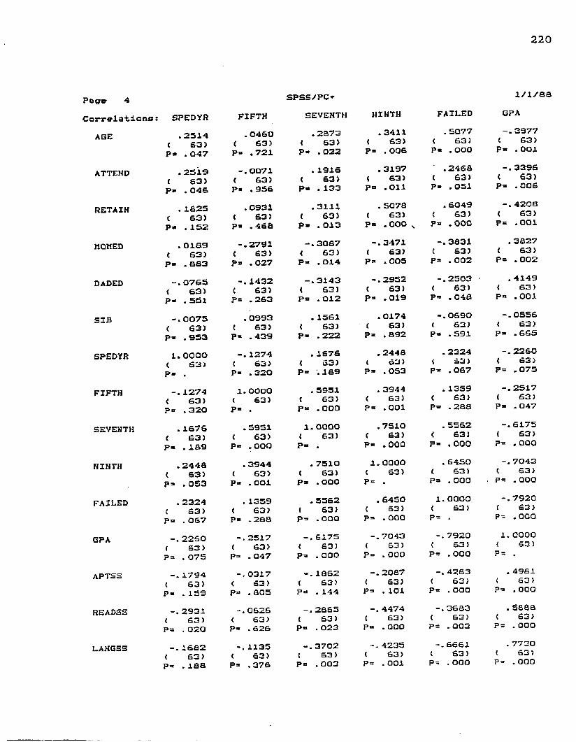
220

Page 4Correlations: SPEDYR

AGE

ATTEND

RETAIN

HOMED

DADED

SIB

SPEDYR

FIFTH

SEVENTH

NINTH

FAILED

GPA

APTSS

READSS

LAHG5S

. 2514 ( £3>P« .047

. 2519 ( 63)P- .046

. 1625 ( 63)P- .152

. 0139 ( 63)P= .333-. 0765

( 63)P- .551

0075 ( 63)P- .9531.0000

< 63) P» •

1274< 63) P» .320

. 1676 ( 63)pa .169

. 244a< 63) Pa .053

. 2324 ( 63)P = .067

2260 ( 63)Pa .075-.1794

< 63) P= .159-. 2931

( 63)pa .020

1662 ( 63)pa .iaa

FIFTH. 0460

( 63)P= .721

-.0071< 63) P- .956

.0931 4 63)Pa .466

-.2791 ( 63)P= .027

-. 1432 t 63) Pa .263

. 0993 ( 63)P* .439

-.1274 4 63)P- .320

1 . OOOO< 63) P= .

.5951 ( 63)Pa .OOO

.3944 C 63)pa .aoi

. 1359< 63) pa .2aa

-.2517< 63) P= .047

-.0317< 63)p» . aos

0626 ( 63)Pa .626

1135 ( 63)Pa .376

SPSS/PC*SEVENTH

.2673< 63) Pa .022

. 1916 ( 63)Pa .133

. 3111 ( 63)P- .013

-.3067 ( 63)Pa .014

-.3143< 63) Pa .012

. 1561 ( 63)Pa .222

. 1676 ( 63)Pa '. 169

. 5951 { 63)P= . OOO

1.0000 t 63) P- .

. 7510 ( 63)Pa .OOO

. 5562 ( 63)P= . QQO

-.6175< 63)Pa .000

ia62 ( 63)pa .144

2665 ( 63)pa .023

3702 t 63) pa .003

NINTH. 3411

{ 63)Pa .006

. 3197 ( 63)Pa .011

. 5076 ( 63)Pa .OOO ^

-.3471 t 63) pa .005-.2952

( 63)Pa .019

. 0174 ( 63)Pa .392

.2446( £3)Pa .053

. 3944 ( 63)Pa .001

. 7510 ( 63)pa . 0001.OOOO

( 63)P» .

.6450 < 63)P= .OOO

7043 ( 63)P= .OOO-.2087

( £3)P= .101

4474 ( 63)P= .OOO

4235 C 63)Pa .OOl

FAILED. 5077

( 63)pa .OOO

.2468 ( 63)P- .051

. 6049 t 63) pa .000-. 3831 ( 63)Pa .002-.2503

( 63)pa .048-. 0690

( 63)Pa .591

. 2324< 53) P« .067

. 1359 ( 63)P= .238

. 5562< 63) P- .000

. 6450 t 63) pa . oao

i .oaoo( 63)P= .

7920 ( 63)p= .ooo

4263< 63) P= .OOO-.3683

( 63)p a .003

6661 ( 63)P= .OOO

l / i / a a

G P A

- . 3 9 7 7

( 6 3 )

p a . OOl

- . 3 3 9 6

< 6 3 )

P a . 0 0 6

- . 4 2 0 0

( 6 3 )

p a .OOl

. 3 8 2 7

( 6 3 )

p a . 0 0 2

. 4 1 4 9

( 6 3 )

P a . 0 0 1

- . 0 5 5 6

{ 6 3 )

P a .665- . 2 2 6 0

t 6 3 )

P a . 0 7 5

- . 2 5 1 7

( 6 3 )

P a . 047- . 6 1 7 5

< 6 3 )

P = .OOO

- . 7 0 4 3

< 6 3 )

P a . 0 0 0

-.7920 C 63)P= .OOO

1 . OOOO t 53)

P a .

. 4961< 63) p - . OOO

. 5 8 8 6

( 63)P a . OOO

. 7730 { 63)

P = . OOO

Page 5 SPSS/PC i/i/aaC o r r e l a t i o n s : SPEDYR FIFTH S E V E N T H NINTH F A I L E D C P A

M A T H S S osoa - . 0 6 7 9 - . 3 7 3 3 - . 3 4 0 9 6 0 3 4 . 6 2 4 4

( 6 3 ) ( 6 3 ) ( 6 3 ) ( 6 3 ) ( 6 3 ) ( 6 3 )

P « . 6 9 2 P " . 5 9 7 P " . 0 0 3 P » . 0 0 6 P = - . 0 0 0 P= .COOTQTALSS - . 2 2 7 3 - . 0 9 2 0 - . 3 7 6 3 -. 4 7 1 A -.sasa . 7 4 5 1

( 63) ( 6 3 ) ( 6 3 ) ( 6 3 ) ( 6 3 ) ( 6 3 )

P » . 0 7 3 P « . 4 7 3 P » . 0 0 2 P » . O O O P = . 0 0 0 P « . 0 0 0

( C o e f f i c i e n t . / ( C a a v a ) / 2 - t a i l e d S i g n i f i c a n c e )

* . * i s p r i n t e d i f a c o e f f i c i e n t c a n n o t b e c o m p u t e d

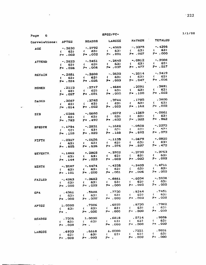
222

Page 6 C o r r e l a t i o n s s

A G E

A T T E N D

R E T A I N

H O M E D

D A D E D

S I B

S P E D Y R

F I F T H

S E V E N T H

N I N T H

F A I L E D

G P A

A P T S S

READSS

L A H G S S

5 P S S / P C -

A P T S S

3 6 3 0

( S 3 )

P < * . 0 0 3

- . 2 6 2 3

( 6 3 )

P « . 0 3 8

- . 2 8 5 1

< S 3 )

P > . 0 2 4

. 2 1 1 3

( S 3 )

P = . 0 9 7

. 3 0 8 7

( S 3 )

p a . 0 1 4

. 0 3 8 8

( 6 3 )

P » . 7 S 3

1 7 9 4

f S 3 )

P a . 1 5 9

0 3 1 7

t S 3 )

P a . 8 0 5

1 8 6 2

( S 3 )

P a . 1 4 4

2 0 8 7

i S 3 )

pa .loi

4 2 6 3

( S 3 )

P a . O O O

. 4 9 6 1

< 6 3 )

P a . O O O

1 . O O O O

< 6 3 )

P= .. 7 3 0 6

t S 3 )

P = . O O O

. 6 9 3 3

< S 3 )

p = . O O O

R E A D S S

3 7 9 2

i S 3 )

p a . 0 0 2

- . 3 4 5 1

< S 3 )

pa . 0 0 6

- . 2 8 0 0

< S 3 )

p - . 0 2 6

. 2 7 1 7

( S 3 )

P » . 0 3 1

. 3 7 8 2

( S 3 )

P« . 0 0 2

0 8 8 0

t 6 3 )

p a . 4 9 3

- . 2 9 3 1

( S 3 )

P- . 0 2 0

0 6 2 6

( S 3 )

P a . 6 2 6

2 8 6 5

< S 3 )

pa . 0 2 3

- . 4 4 7 4

{ S 3 )

P - . 0 0 0

- . 3 6 8 3

< S 3 )

pa . 0 0 3

. 5 8 8 8

( 6 3 )

Pa .OOO, 7 3 0 6

( 6 3 )

pa .0001.OOOO ( 63)P» .

. 6 8 1 8

( 6 3 )

Pa .000

L A N G S S

- .4069 ( S3)P= .OOl

- .2640 t S3) P» .037

- .3630 t S3) P- .003

.4684 ( S3)pa .OOO

. 3744 t S3) P« .003

. 0272 ( 63)Pa .832

- .1682 ( 63)P° .188

- .1135 < 63 >pa .376

- .3702 ( 63)P» .003

- .4235 ( 63)Pa .a o i

- .6661( S3)Pa .000

. 7730 ( 63)Pa .OOO

. 6933 ( 63)Pa .OOO

. 6818 ( 63)P= .OOO

1 . OOOO ( S3)P= .

M A T H S S

- . 3 3 7 5

< S 3 )

Pa . 0 0 7

- . 0 9 1 2

< 6 3 )

Pa . 4 7 7

- . 2 5 1 4

t 6 3 )

P= . 0 4 7

. 2 0 9 1

( S 3 )

Pa . 1 0 0

. 1 7 8 5

< 6 3 )

P= . 1 6 2

. 1 2 6 9

( 6 3 )

pa . 3 2 2

- . 0 5 0 8

( 6 3 )P= . S 9 2

- . 0 6 7 9

( 6 3 )

Pa . 5 9 7

- . 3 7 3 3

t 6 3 )

pa . 0 0 3

- . 3 4 0 9

i 6 3 )

pa . 0 0 6

- . 6 0 3 4

< 6 3 )

p= ,OOO. 6 2 4 4

( S 3 )

pa .OOO. 6 7 3 0

( S 3 )

p= .OOO. 5 7 1 4

( 6 3 )

pa .OOO. 7 2 2 1

( 6 3 )

pa .OOO

TOTALSS

-.4298< 63) Pa . OOO

-.3008< 63) P= .017

-. 3419 ( 63)Pa . QOS

. 3691< S3) pa .003

. 3800< 63) P= .002

-.0061< 63) pa .962

-.2273 ( S3'Pa .073

-.0920 ( 63)P“ .473

-.3763 ( 63)P= .002

-.4711< 63) P» .000

-.5838 ( 63)P= .000

. 7451< 63) P= . OOO

. 7982 ( 63)P= . OOO

. 9086 ( 63)Pa . OOO

. 9031 ( 63)Pa . 000

1 /1/88

(Coefficient. / (Cases)

/ 2-tailed Significance)

Dc&4a

HO2rtnto

o *00 a

sc U)> q-t Qa Htn Dtn 1+ M

M-0s&•*

D ~ *0 -1 II >■« • nva in Homm o m vi tn

OUD o u u inO - M o ~ o

*0 - u -* » 50MID * Ul >O (T> 0 O ft vl O□ u is ou t- ino — m o v ii> in

*0 ~ D -a * rt * >■in vj xo m o o m u ClD U U 01)10 tnO - M 0-1- tn

u - TP -a U V* a« * >

(S o Ho m o m o XO U 1- u o tnO - L) — o in

*0 - t -B k> H H* * □o ffi H

tn o o tn o >■U D o u p- o o - u in

tnT)tnins•flO+

tn

i-ists

223

APPENDIX LMULTIPLE REGRESSION ANALYSIS AND PLOTS ON NINTH GRADE DATA

224

225

Page 15 s p s s /p c * i/i/aaM U L T I P L E R E G R E S S I O N * . * *

Dependent. Variable. . NINTH ninth grade absenteeism ratEquation Number 1 Beginning Bloch Number 14. Method: Enter SIB

Variable(s) Entered on Step Number14.. SIB number of siblings residing in home

Multiple R .08942R Square .79108Adjusted R Square .73013Standard Error 5.75568.Analysis of VarianceRegressionResidual

DP Sum of Squares14 6020.5349848 1590.13930

Mean Square 430.03821 33.12790

12.98115 Signif F .0000

Variables in the EquationVariable B SE B Beta T Sig TSEVENTH 1.07360 .25516 .48409 4. 208 . 0001GPA -4.31788 1.38358 -.42463 -3.121 . 0031RETAIN 6.10999 2. 05719 .26589 2. 970 . 0046READSS 08564 .02687 -.35850 -3.187 . 0025LANGSS .07511 .04665 .23763 1. 610 . 1139FIFTH 03397 .28687 01086 n a . 9062MOMED -. 77170 .58856 11454 -1.311 . I960AGE -1.82501 2.04096 -.08072 -. 894 . 3757MATHSS .03402 .06642 .06274 .*512 . 6109ATTEND .51959 .59091 .06956 . 879 . 3836DADED .68263 .53566 .10490 1. 274 . 2087SPEDYR .04380 .61583 5.4062E-03 . 071 . 9436APTSS .26031 .14825 .20853 1.756 . 0855SIB -1.18334 .78525 -.11185 -1. 507 . 1384(Constant) 14.92997 57.94322 . 258 . 7978

End Slock Number 14 All requested variables entered.

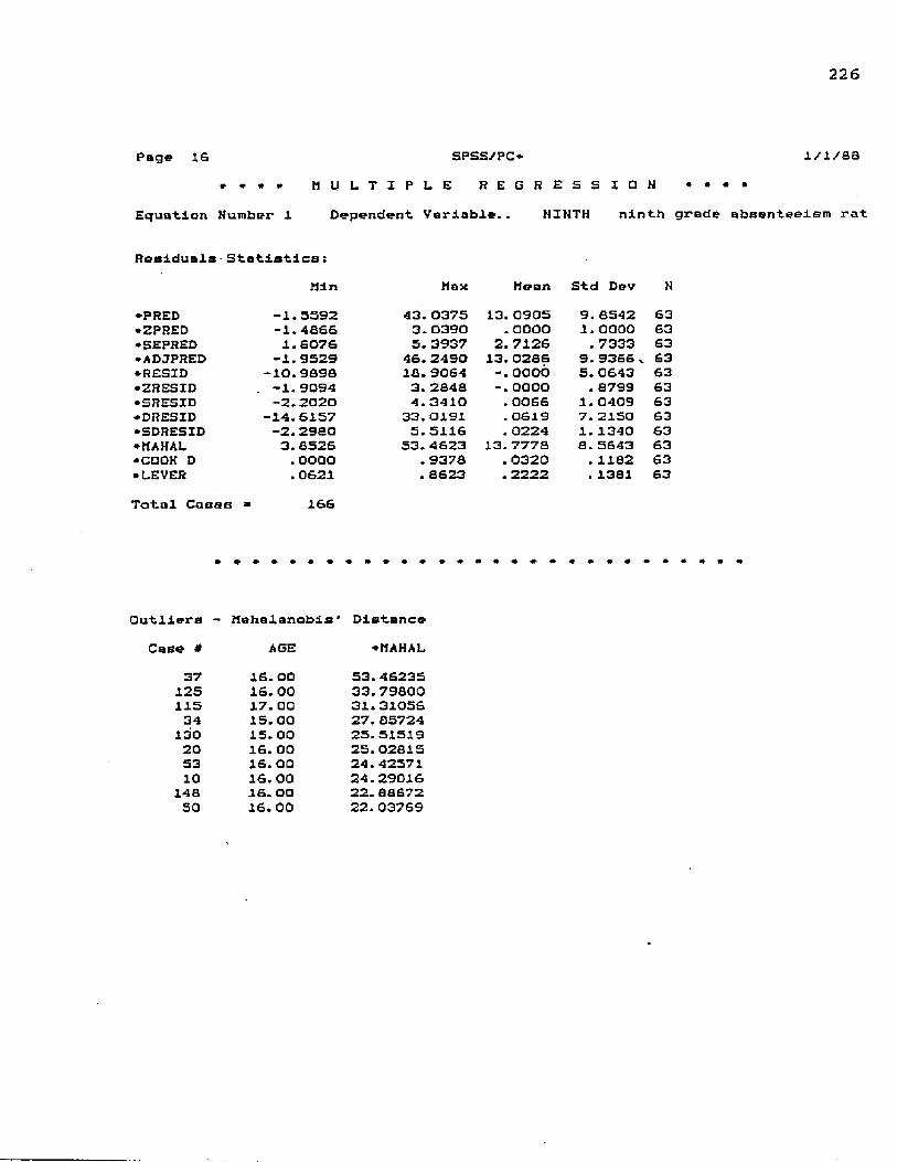
226

Page IS SPSS/PC* 1/1/88* * * * M U L T I P L E R E G R E S S I O N • • • •

Equation Humber 1 Dependent Variable.. NINTH ninth grade absenteeism rat

Residuals - Statistics:Min Max Mean Std Dev N

•PRED -1.5592 43.0375 13.0905 9. 8542 63•ZPRED -1.4866 3.0390 .OOOO 1. OOOO 63•SEPRED 1.6076 5.3937 2. 7126 . 7333 63•ADJPRED -1.9529 46.2490 13.0286 9.9366 k 63•RESID -lO.9898 18.9064 -. OOOO 5.0643 63•ZRESID . -1,9094 3.2848 -.OOOO . 8799 63•SRESID -2.2020 4.3410 . 0066 1. 0409 63•DRESID -14.6157 33.0191 . 0619 7.2150 63•SDRESID -2.2980 5.5116 . 0224 1.1340 63•MAHAL 3.8526 53. 4623 13.7778 8.5643 63•COOK D . OOOO . 9378 .0320 . 1182 63•LEVER . 0621 . 8623 . 2222 . 1381 63Total Casas » 166

Outliers - Jlahalanobls' DistanceCase 4 AGE *MAHAL

37 16.00 53.46235125 16.00 33.79300115 17.00 31.3105634 15.00 27.35724

130 15.00 25.5151920 16.00 25.0231559 16.00 24.4257110 16.00 24.29016

148 16.00 22.38672SO 16.00 22.03769

227

Pago 17 SPSS/PC* l/I/SS

Histogram - Studentized ResidualHExp H (» ” 1 Cases, : Normal Curve)1 . 05 Out •□ . io 3. OOa . 25 2. 67o . 5S 2. 330 1. 15 2.00 *i 2. 11 1. 67 * •5 3. 46 1. 33 • * { •6 5. OS 1. OO • * * : *6 6. 69 . 67 *• ♦a 7. S9 . 33 m- # # -» # *9 8. 34 0. 0 * ♦ # ♦ • ♦a 7. 69 33 • * ♦ • • #e 6. 69 -. 67 • * »6 5. OS -1. OQ • • * : *4 3. 46 -1. 33 *« :1 2. 11 -1. 67 • -1 1. 15 -2. OO s1 . 56 -2. 33 :0 .25 -2. 670 . 10 -3. OOo .05 Out

Normal Probability (P-P) Plot Standardized Residual1. Q

.750bserved

25

. 25

228

Page 18 SPSS/PC* 1/1/88

Standardised ScatterplotAcross - *PHED Down - «SRESID

3 + » Symbols:

-2

Max H1. O2. 0 3. O

-3 *Out **-------------------+ + +■

- 3 - 2 - 1 O 1 2 3 Out

229

Page 19 SPSS/PC* 1 / 1 / a a

Standardized Partial Regression Plot Across - LANGSS Down - HINTH

3 *

-1

-3 + Out +-*■-

-3 -2 -1

Symbols : Max N

1.02. Q

3 Out

Standardized Partial Pogroasi-’-' °lot Across - GPA Dovn - NINTHOut 3 Symbols;

Max N1.02. O3. 0

3 Out

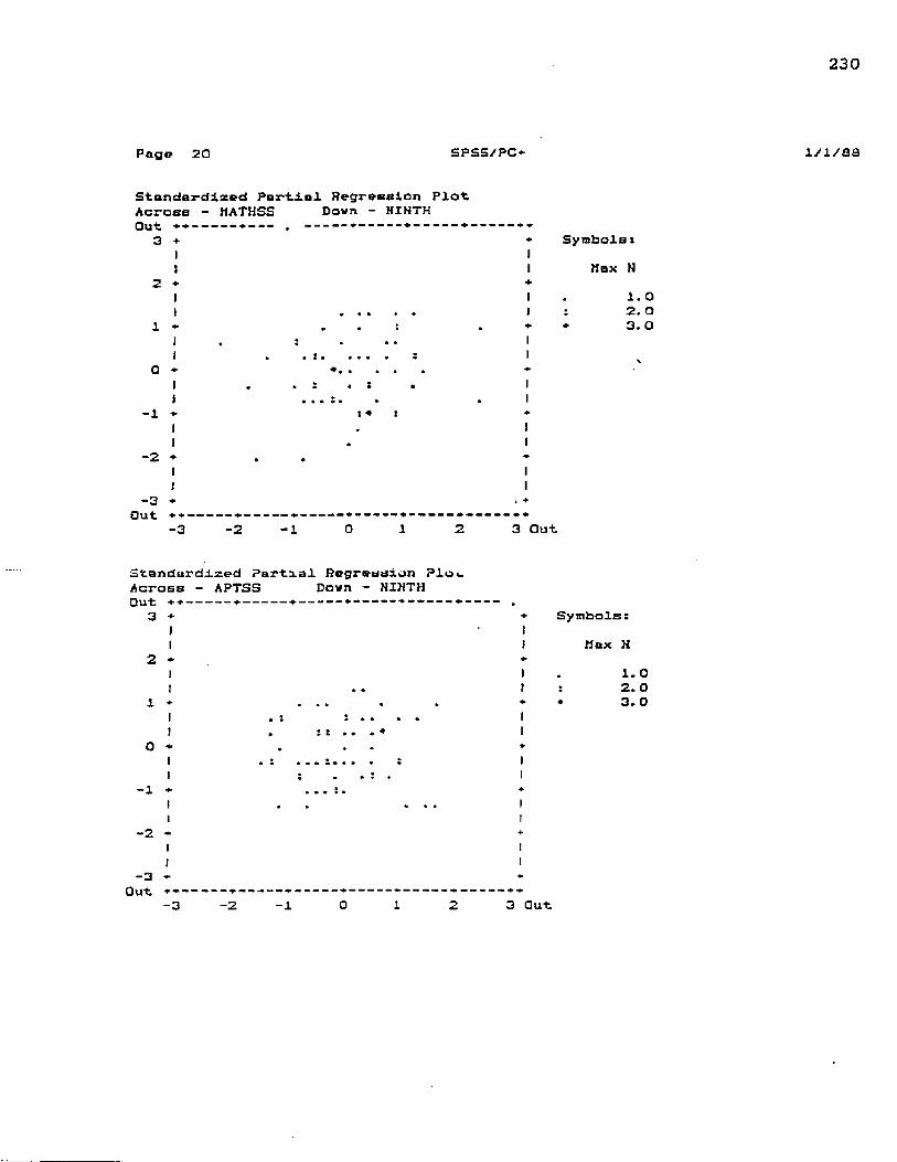
230

Page 20 SPSS/PC- i/i/aa

Standardised Partial Regression Plot Across - MATHSS Dovn - NIHTHOut ----- +---- . -----------

3 +

-3 * Out **•

-3 -2

Symbolsi Max N

1.02. O3. 0

• + +3 Out

Standardised Partial Regression Plot Across - APTSS Dovn - HIHTH

3 * Symbols: Max N

1. □ 2.0 3. O

-2

-3 *Out ------ * ” ------*------------ -

- 3 - 2 - 1 0 1 2 3 Out

231

Page 21 SPSS/PC* 1/1/8S

Standardised Partial Regression Plot Across - SEVENTH Down - HIHTH Out 3

2

1O

-1

-2

-3Out

- 3 - 2 - 1 O 1 2 3 Out

Symbols: Max N

1.0 2. 0 a . a

Standardized Partial Regression Plot Across - READSS Down - NINTHOut **

3 - Symbols:Max N

1. O2.0

3 Out

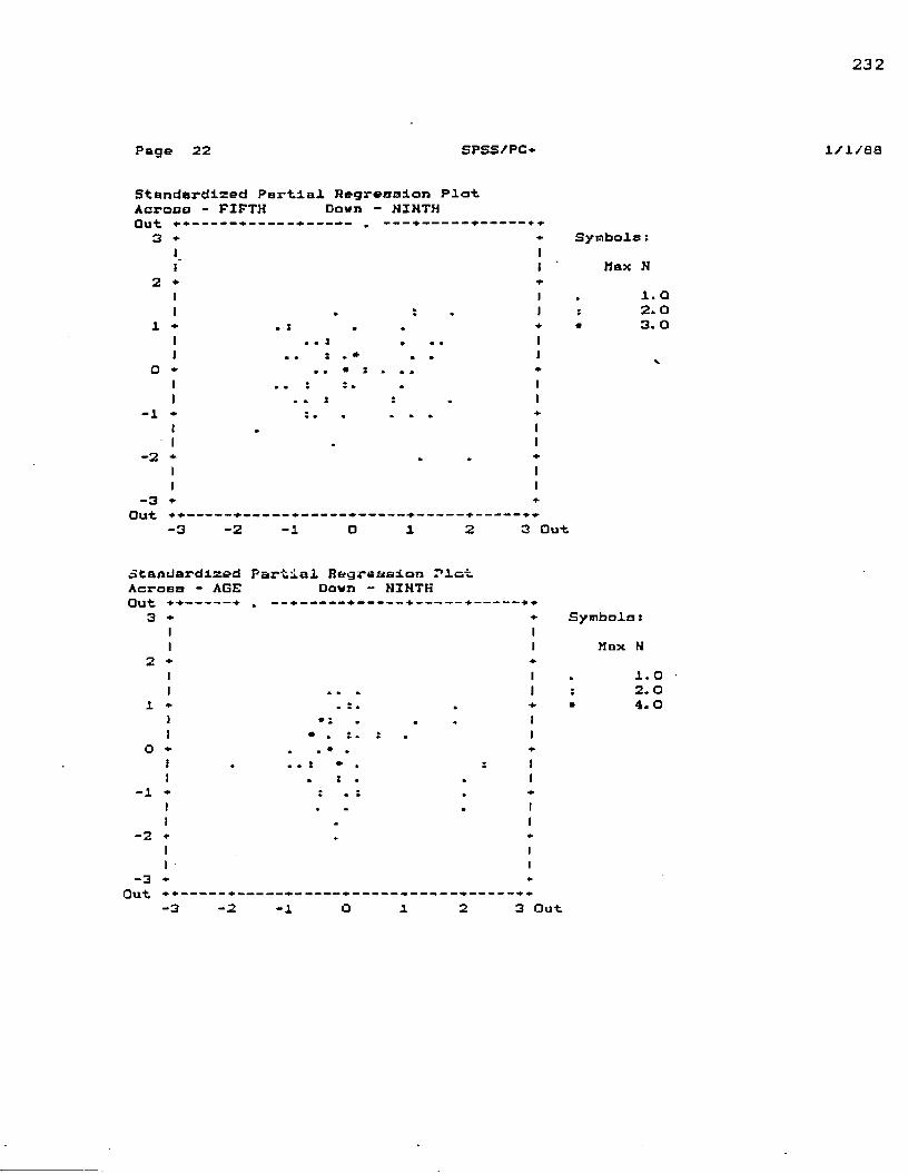
232

Page 22 S P S S / P O 1/1/83

Standardized Partial Regression Plot Across - FIFTH Doan - HIHTHOut +♦---— »----- » ■* ------*-

3 *

-1

-2

-3 * Out ++■ -3

Symbols: Max N

1. O 2* 03. O

-2 -1 3 Out

Standardized Partial Regression Ploi Across - ACE Dovn - NIHTHOut ++----- + . *-------

3 *

-2

Symbols: Max H

1. O2.04. O

-3 * Out ** -3 - 2 - 1 O 1 2

233

Page 23 SPSS/PC* 1/ 1/88

Standardized Partial Regression Plot Across - RETAIN Down - NINTH

3 *

■ * * '. ;s .

- 3 - Out **-

-3 -1

Symbols t Max N

1.02. O4. O

3 Out

Standardized Partial Regression Plot Across - HONED Down - NINTHOut ,

3 *

-1

-2

Symbols: Max N

1. 02. O3. 0

-3 *Qtl't — ~ — - * — — — — — — + — — — + — — — — — + — — — — —

- 3 - 2 - 1 0 1 2 3 Qu-t

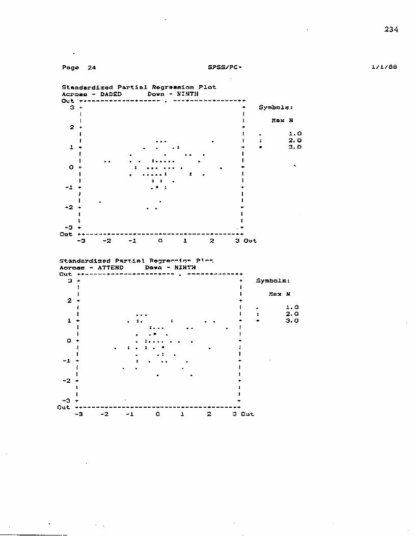
234

Pag® 24 SPSS/PC* i/i/aa

Standardized Partial Regression Plot Across - DADED Dovn - NINTH3 «-

. i

-3 * Out ■n

Symbols; Hex N

1.02. O3. O

-2 -1 3 Out

Standardized Partial Pegra^-i r>" P 1, Across - ATTEND Dovn - NINTH□ut ++- — >•----- ■*---. ------

3 *

-1

-2

-3 -Out *■<•-

-3

Symbols: Max N

1.0 2.03. 0

3 Out

235

Page 25 SPSS/PC-* 1/1/ae

Standardized Partial Regression Plot Across - SPEDYR Down - MIHTHOut **----- *--------- . - +----- * ♦ -

3 *

-3Out

-2 -1

Symbols; Max N

3 Out

1.0 2.03. 0

Standardized Partial Regression Plot Across * SIS Dawn ~ NINTHOut --<■ . *

3 * * Symbols:

-2

> » I 4• . : * •

Max N1.02. 03. 0

-3 +Out ----- •*----- + + *

- 3 - 2 - 1 0 1 2 3 Out

APPENDIX MDISCRIMINANT ANALYSIS AND PLOTS ON NINTH GRADE DATA

236

237

Page SPSS/PC+D I S C R I M I N A N T A N A L Y S I S

□n groups defined by GROUP group assignment166 Cunweighted) cases were processed.103 of these were excluded from the analysis.

0 had missing or out-of-range group codes.103 had at least one missing discriminating variable.

63 Cunweighted) cases will be used in the analysis.Number of Cases by Group

Number of CasesGROUP Unwei ghted Weighted Label

1 13 13.0 female attender '2 24 24.0 male attender3 13 13.0 female nonattender4 13 13.0 male nonattender

Total S3 63. 0Group means

GROUP AGE ATTEND RETAIN MOMED1 15.00000 4.07692 .00000 13.07692r> 15.00333 3.97500 .00000 13.00000

15.30769 4.38462 .23077 11.615384 15.61539 5.07692 .53846 11.69231

Total 15.22222 4.269S4 .15873 12.46032GROUP DADED SIB SPEDYR FIFTH

1 12.76923 1.61530 .00000 4.346152 12.70033 1.50000 .00oo^ 4.412503 11.46154 1.84615 .00000 6.861544 11.39462 1.94615 1.07692 6.10769

Total 12.19049 1.66667 .25397 5.25397GROUP SEVENTH NINTH FAILED GPA

1 5.07692 6.06154 .84615 2.933852 4.59167 5.93555 1.54167 2.496673 10.1230S 20.19231 7.00000 1.506154 12.00769 26.41538 14.92309 .72539

Total 7.36349 13.09049 5.28571 1.99254GROUP APTSS READSS LANGSS MATHSS

1 51.23077 765.69231 732.00000 724.3046252.54167 765.83333 725.04167 731.4166744.76923 725.46154 707.53846 719.15395

4 44.76923 722.46154 693.23077 707.3076?Total 49.06349 749.52391 714.23910 722.25397

Group Standa rd DeviationsGROUP AGE ATTEND RETAIN MOMED

1 .00000 1.25576 .00000 1.33212.40925 1.26190 .00000 1.39913™ .63043 1.30455 .59914 1.12090

4 .50637 1.55250 .77625 1.25064Total .49004 1.49331 .48214 1.64440

1/1/S0

238

Page 3 S P S S / F O 1/1/SOGROUP DADED SIB SPEDYR FIFTH

1 1.69005 1.04391 .00000 2.742752 1.S0529 1.06322 .40825 3.679123 1.39137 1.06019 .00000 3.738444 1.32530 1.06819 2.90004 3.38611

Total 1.70253 1.04727 1.36746 3.54163GROUP SEVENTH NINTH FAILED GPA

1 3.39605 2.70109 1.57301 .022602 3.S3144 3.57232 3.17571 .825093 4.25013 6.79098 6.49359 .76306i4 4.30022 12.26011 B.94857 .56499

Total 4.99572 11.07939 7.50485 1.08958GROUP APTSS READSS LANGSS MATHSS

L 0.09479 47.90161 29.22043 15.036202 7.60994 36.58090 29.94412 16.730393 S.6S095 39.50060 32.08519 24.575994 9.26601 49.61622 32.07843 18.91377

Total 8.87525 46.37952 35.05282 20.43398Pooled Within-Graups Correlation Matrix

AGE ATTEND RETAIN MOMED DADED SIB SPEDYRAGE 1.OOOOOATTEND .10703 l.OCOCORETAIN .49697 -.01834 1.00000MOMED .12420 -.01410 -.06720 1.00000DADED .03920 — .19846 — • 04934 . 3567-i 1.00000SIB -.07731 -.16766 -.16111 -.10413 -.04911 1.OOOOOSPEDYR .14910 .10611 .07000 .10208 -.00632 -.03411 1.00000FIFTH -.07300 -.00095 -.01039 -.18010 -.03667 .06053 -.17835SEVENTH .00931 .00944 .05523 —.07387 -. 10482 .00410 .03716NINTH -.03163 .15289 .30151 -.04984 .00722 -.16139 .10809FAILED .28526 .04729 .45690 -.19037 -.00630 -.23137 .05168GPA -.10303 -.20221 -. 16098 .16422 .23823 .05615 ** -. 06850APTSS 24505 -. 17555 -.15118 .05159 .18255 .11123 -.12562READSS -.24037 -.26369 -. 12310 .10646 .25107 -.02618 -.24602LANGSS -.22229 -.13997 -. 177B3 .36119 .24012 .10610 -.03599MATHSS -.18696 .05240 -.07494 .06233 .03344 .21391 .06986

FIFTH SEVENTH NINTH FAILED GPA APTSS READSSFIFTH 1.00000SEVENTH .57257 1.00000NINTH .31155 .52153 1.00000FAILED -.04022 .22445 .21038 1.00000GPA -.10270 -.31773 -.32414 -.58576 1.00000APTSS .10133 .10235 .20149 -.26742 .35940 1.OOOOOREADSS .07905 — .00530 -.17697 -.12582 .45648 .67239 1.OOOOOLANGSS .00605 -.09208 -.05667 -.50223 .68481 .65374 .61705MATHSS .04105 -.14710 -.00360 -.40296 .54112 .62013 .40974

LANGSS MATHSS LANGSS 1.00000MATHSS .66922 1.00000Correlations which cannot he computed are printed as

239

Page 4 5PSS/PC+Wilks' Lambda (U—statistic) arid univariate F-ratia with 3 and 59 degrees of freedomVariable Wilks' LambdaAGEATTENDRETAINMOMEDDADEDSIBSPEDYRFIFTHSEVENTHNINTHFAILEDGPAAPTSSREADSSLANG5SMATHSS

.73444

.90569

.80053

.82773

.35454

.97733

.90357

.90399

.59172

.36009

.43462

.47001

.82937

.79930

.73766

.79927

F5. 4042. 048 4. 399 4. 0933. 348 . 4552 2. 099 1. 969 13. 57 34.95 20.91 22. 134. 032 4.938 6.994 4. 939

Significance.0024 . 1169 .0042 .0105 .0250 .7146 . 1100 . 1284 . OOOO . OOOO .0000 .0000 .0112 .0040 . 0004 . 0040

I/1/SO

240

Page 5 SPSS/PC+ 1/1/80— ------------------— d i s c r i m i n a n t a n a l y s i s -----------------------------------------

On groups defined by 6RQUF group assignmentAnalysis number 1Stepwise variable selection

Selection rule: Minimice Wilks' LambdaMaximum number of steps..................... 32Minimum Tolerance Level.......... .00100Minimum F to enter........................... 1.0000 ^Maximum F to remove.............. 1.0000

Canonical Discriminant FunctionsMaximum number of functions................ 3Minimum cumulative percent of variance... 100.00Maximum significance of Wilks’ Lambda.... 1.0000

Prior probability for each group is .25000------------- — — Variables not in the analysis after step 0

Variable ToleranceMinimum

Tolerance F ta enter Wilks' LambdAGE I.0000000 I.ooooooo 5.4042 .78444ATTEND 1.0000000 1.0000000 2.0478 .90569RETAIN 1.0000000 1.ooooooo 4.8990 .8005aM0MED 1.0000000 1.0000000 4.0932 .82773DADED 1.0000000 1.0000000 3.3476 .B5454SIB 1.ooooooo 1.ooooooo .45525 .97738SPEDYR 1.ooooooo 1.ooooooo 2.09S9 .90357FIFTH 1.0000000 1.ooooooo 1.9691 .90899SEVENTH 1.ooooooo 1.0000000 13.570 .59172NINTH 1.ooooooo 1.0000000 34.949 .36009FAILED 1.ooooooo 1.0000000 20.915 .48462GPA 1.ooooooo 1.ooooooo 22.177 .47001APTSS 1.ooooooo 1.0000000 4.031S .82937READSS 1.ooooooo 1.0000000 4.9333 .79930LANGSS 1.ooooooo 1.0000000 6.9942 .73766MATHSS 1.ooooooo 1.0000000 4.9392 .79927* * * * * i t : : : * * * * * * * * * * * * * * * * * * * *At step 1, NINTH was included in the analysis.

Degrees of Freedom Signif. Between Groups Wilks’ Lambda .36009 I 3 59.0Equivalent F 34.9489 3 59.0 .0000— —-----------------Variables in the analysis after step 1 -------------------Variable Tolerance F to remove W i l k s ’ LambdaNINTH 1.0000000 34.949

241

Page SPSS/PC+ i/i/aoVariables not in the analysis a-fter step

MinimumVariable Tolerance Tolerance F to enter Wilks' LambiAGE .9939995 .9939995 2.4663 .31935ATTEND .9766261 ,9766261 ,23931 .35477RETAIN .9090939 .9090939 .3797a .55316MOMED .9975155 .9975155 1.2602 .33806DADED .9999473 .9999478 1.3198 .33708SIB .9739541 .9739541 .97039 ,34208SPEDVR .9383156 .9883156 1.0189 .34207FIFTH .9029350 .9029358 .55046 .34998SEVENTH .7279580 .7279530 .23585 .35575FAILED .9523109 .9523109 5.1283 .28460GPA .0949357 .8949357 3.8294 .30056APTSS .9594027 .9594027 3.8911 .29976READSS .9686799 .9686799 .63958 .34056LANGSS. .9967880 .9967880 2.2439 .32265MATHSS .9999871 .9999071 2.0445 .32565* * * * * * * * * * * * * * * * * * * * * * * * * * * * *At step 2, FAILED was included in the analysis.

Wilks' Lambda Equivalent F

.29460 16. W i ’

Degrees of Freedom Signif. 2 3 59.0

6 116.? ,0000Between Groups

------------------- Variables in the analysis a-fter stepVariable Tolerance F to remove NINTH .9523109 13.538FAILED .9523109 5.1203

Wilks' Lambda .4B462 .36009

Variables not in the analysis after stepMinimum

Variable Tolerance Tolerance F to enter Wilks’ Lamb.AGE .9093623 .8660629 .76105 .27364ATTEND .9764230 .9319420 .22830 ,20122RETAIN .7484410 .7404410 .35635 .27936MDMED .9606050 .9170738 .97061 .27066DADED .999S814 .9522366 1.1613 .26020SIB .9335606 .9128150 1.5874 .26266SPEDYR .9874076 .9429140 .01508 .272BSFIFTH .3906209 .3495300 .25462 .20OS4SEVENTH .7151245 .7151245 .10035 .20193GPA .6164525 .6164525 1.2426 .26713APTSS .0575643 .0512253 2.6461 .24901READSS .9606995 .9296013 .52197 ,27699LANGSS .7447683 .7115u/0 .25636 .20110MATHSS .7550539 .7190172 .87243 .27211

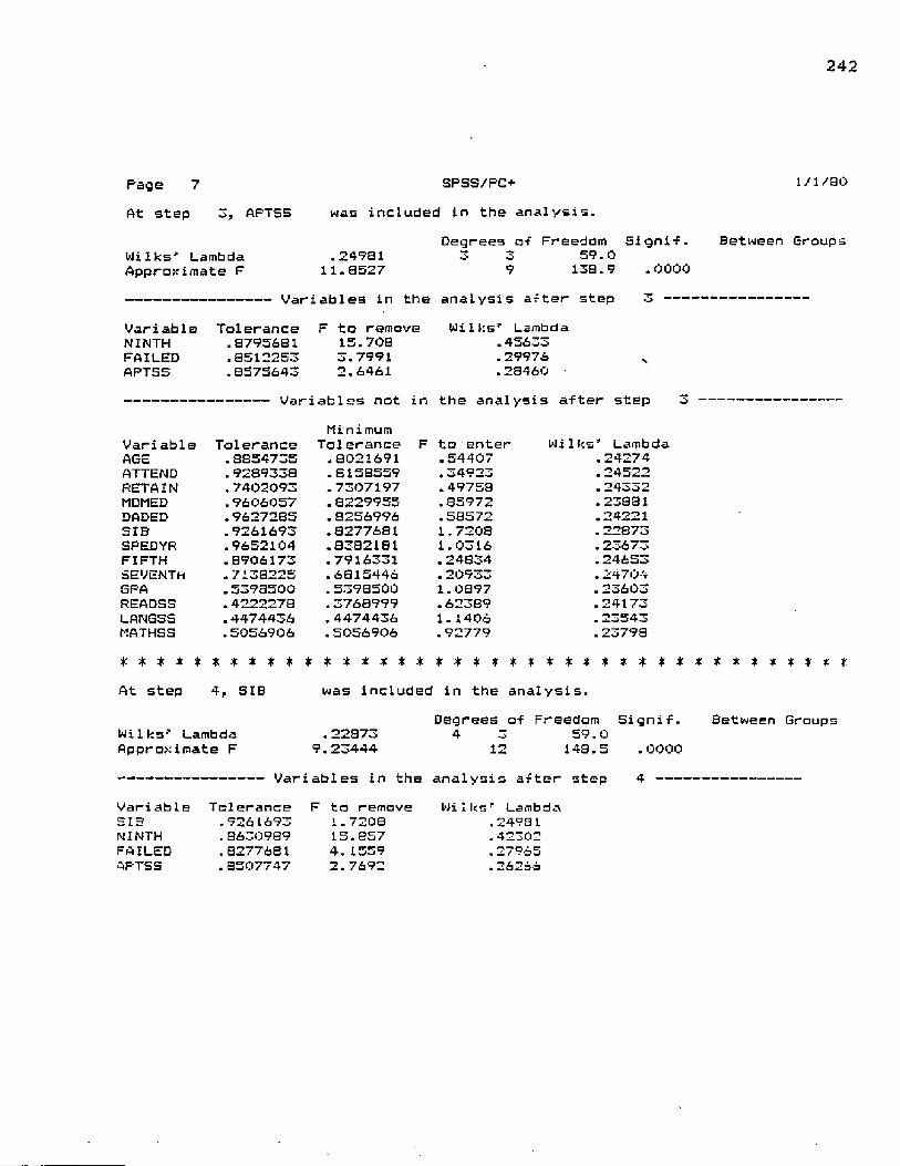
242

Page 7 At step 3, APTSS

Wilks' Lambda Approximate F

S P S S / P Owas included in the analysis.

Degrees of Freedom 5ignif. .24981 3 3 59.0

11.8527 9 138.9 .0000Variables in the analysis after step

Variable Tolerance F to removeNINTH .8795681 15.708FAILED .8512253 3.7991APTSS .B57S643 2.6461

Wilks' Lambdi .45633 .29976 .28460

Variables not in the analysis after step Minimum

Vari able Tolerance Tolerance F to enter Wilks LambAGE .8854735 .8021691 .54407 .24274ATTEND .9289338 .815B559 .34923 .24522RETAIN .7402093 .7307197 .49758 .24332M0MED .9606057 .8229955 .85972 .23831DADED .9627285 .8256996 .58572 .24221SIB .9261693 .8277681 1.7208 .22873SPEDYR .9652104 .8382181 1.0316 .23673FIFTH .8906173 .7916331 .24834 .24653SEVENTH .7138225 .6815446 .20933 .24704GPA .5398500 .539B500 1.0B97 .23603READSS . 422227B .3768999 .62389 .24173LANGSS .4474436 .4474436 1.1406 .23543MATHSS .5056906 .5056906 .92779 .23798* * * * * * * * * * * # * * * * * £ £ * Y # * * # * * * #At step 4, SIB was included in the analysi s.

1/ 1/80

Between Groups

Wilks' Lambda Approximate F

Degrees of Freedom Signif. .22873 4 3 59.0

9.23444 12 148.5Between Groups

Variables in the analysis after step. 0000 4 ----

Variable Tolerance F to removeBIB .9261693 1.7208NINTH .8630989 15.B57FAILED .B277681 4.1559APTSS .8507747 2.7692

Wilks' Lambda .24931 .42302 .27965 .26266

243

Page SPSS/PC+ 1/ 1/aoin the analysis after step 4

MinimumVari able Tolerance Tolerance F to enter Wilks' LambdaAGE .8853B70 .7sieaes .52139 .22240ATTEND .9130253 .8130463 .36062 .22431RETAIN .7395S24 .7156563 .40719 .22376MOMED .9360473 .7921955 .66401 .22073DADED .9SB0033 .0172942 .42717 .22352SPEDYR .9652063 .0273975 1.0132 .21675FIFTH .8822145 .7712597 .28665 .22520SEVENTH .6756042 .6450935 .16776 .22665GPA .5227030 .5227030 1.0910 .21500READSS ,4023201 .3505900 1.0527 .21630LANGSS .4446546 .4446546 1.2183 .21447MATHSS .5002442 .5002442 .83106 .21800* * * * * * * t * * it * * * * * * * * * * * * * * * * * * * * :

At step 5, LANGSS was included in the analysis.Degrees of Freedom Signif.

Mi Iks' Lambda .21447 5 3 59.0Approximate F 7.57767 15' 152.2 .0000

1 J . , ^16 analysi s arter- steD 5Variable Tolerance F to remove Wilks' LambdaSIB .9203963 1.7911 .23543NINTH .0422955 16.299 .40515FAILED .6071764 3.2315 .25220APTSS .5079555 3.0576 .25960LANGSS .4446546 1.2103 .22873

* * * * * * * *

Between Group'

Variables not in the analysis after step 5 — Mi nimum

Variable Tolerance Tolerance F to enter Wilks’ LambdaAGE .0051617 .4445415 .51366 .20052ATTEND .9127024 .4444974 .34501 .21043RETAIN .7219371 .4340459 .55047 .20011MDMED .7915865 .3760300 1.4062 .19012DADED .9165854 .4254306 .62S63 .20724SFEDYR .9553073 .4401312 1.1300 .20 ISOFIFTH .0BO3234 .4437015 .29406 .21103SEVENTH .6751775 .4443212 .17639 .21239GPA .3391519 .3310450 .00750 .20440READSS .3405710 .3333507 .57100 .20787MATHSS .4481905 .3993B54 1.1103 .20193

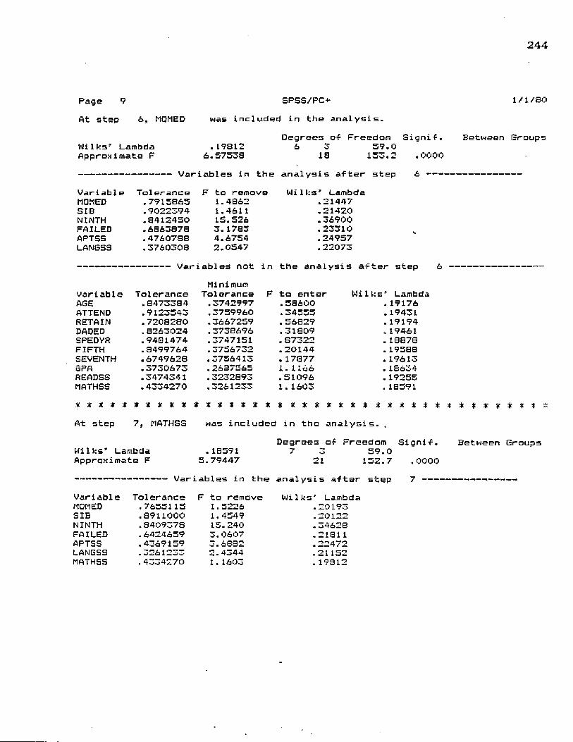
244

Page 9At step - 6, MQMED

S P S S / P O was included in the analysis.

Degrees of Freedom Signif.

l/i/ao

Between GroupsWiIks” Lambda . 19812 6 3 59.0Approximate F 6 * 575oS 18 153.2 .0000

i ^ i.C t < m i ] f a i a a i l c i a i , c p u

Variable Tolerance F to remove Uli 1 ks ’ LambdaMQMED .7915S65 1.4862 .21447SIB .9022394 1.4611 .21420NINTH .S412450 15.526 .36900FAILED .6863878 3.1783 .23310APTSS .4760788 4.6754 . 24957LANGSS .3760308 2.0547 .22073----------------- — --------- Variables not in the analysis after step 6

MinimumVariable Tolerance Tolerance F to enter Wilks' LambdaAGE .B4733S4 .3742997 .58600 .19176ATTEND .9123543 .3759960 .34555 .19431RETAIN .7208280 .3667259 .56829 . 19194DADED .8263024 .3738696 .31809 .19461SPEDYR .9481474 .3747151 .87322 . 18878FIFTH .8499764 .3756732 .20144 .19588SEVENTH .6749628 .3756413 .17877 .19613SPA .3730673 .2637565 I . 1166 .18634READSS .3474341 . 3232893 . 51096 .19255MATHSS . 4334270 .3261233 I . 1603 . 18591* * * * * * * * * * * * * * * * * * * * * * * * * * * * * * *

At step 7, MATHSS was included in the analysis. .Degrees of Freedom Signif.

Wilks’ Lambda . IB591 7 5 59.0Approximate F 5.79447 21 152.7 .0000

. ^0 1 1 0 1 / ^ 4 3 < = * T L. £Sf I — — — — -

Variable Tolerance F to remove W i l k s ’ LambdaMQMED . 7655115 1.5226 20193SIB .8911000 1.4549 20122NINTH .8409378 15.240 *34628FAILED .6424659 3.0607 2181 1APTSS .4369159 3.6882 *22472LANGSS .3261233 2.4344 21152MATHSS .4334270 1.1603 *19812

Between Groups

245

Page 10 SPSS/PCH-Variables not in the analysis after step

Minimum

1/1/SO

Variabie Tolerance Tolerance F to enter Wilks' LambdaAGE .8392931 .32293S6 .5203B .18049ATTEND .8374910 .3216239 .55965 .18009RETAIN .6774840 .3249196 .65720 .17911DADED .8144019 .3218403 .30340 .1B271s p e d y r *8984919 .3258501 • 85638 .17715FIFTH .8475611 .3253667 .20834 .18370SEVENTH .6445577 .3253600 .12504 .18457GPA .3669118 .2512084 1.2966 .17297READSS .3451649 .2941991 .53004 .18039* * * * * * * * * * * * * * * * * * * * * * * * * * * * * *

At step a, gpa Mas included in the analysis.

* * * * * * * * * *

Ulilks' Lambda Approximate F

Degrees of Freedom Signif* .17297 S 3 59.0

S .24429 24 151.4 .0000Between Groups

------------------- Variables in the analysis after step 8VariableMQMEDSIBNINTHFAILEDGPAAPTSSLANGSSMATHSS

Tolerance .7408660 .8538747 .7415467 .571S014 .36691 IS .4323597 .2512084 .4262755

to remove1.65511.30069.74382.42721.29663.78282*04421.3400

Milks' Lambda .1894S .18595 .27020 .19719 .18591 .21071 .19337 .18634

Variables not in the analysis after step Minimum

a

Variable Tolerance Tolerance F to enter Wilks' LambdaAGE .8128952 .2437495 .71263 .16601ATTEND .7991529 .2512079 .88033 ■ 16445RETAIN .6539143 .2508719 .43205 .16868DADED .7561383 .2510120 .28476 .17012SPEDYR .8974352 .2511881 .86070 .16463FIFTH .840298B .2493186 .19381 .17102SEVENTH .6378708 .2491088 .10829 .17187READSS .3412989 .2375554 .55680 .16748F level or tolerance □r VIN insufficient for further computat:

Summary TableActi on Vars W i l k s ’

Step Entered Removed In Lambda Sig. Label1 NINTH I .36009 .0000 ninth grade absenteeism rate

FAILED .23460 . 0000O APTSS O’ .24981 . 0000 academic aptitude standard score4 SIB 4 .22873 . oooo number of siblings residing in homeCT LANGSS 5 .21447 .0000 language achievement expanded stands6 MQMED 6 . 19812 . 0000 m o t h e r ’s educational level7 MATHSS 7 .18591 . 0000 mathematics achievement expanded staa GPA . S .17297 . 0000 grade point average

Page 11 S P S S / P O 1/1/30Canonical Discriminant Functions

Pet of Cum Canonical After Wilks'Fen Eigenvalue Variance Pet Corr Fen Lambda Chisquare DF Sig

: 0 . 1730 93.261 24 . 00001* 3.0349 SS. 97 03.97 .0690 : 1 . 7066 19.452 14 . 14342* .2526 7.29 96.25 .4491 • *T> .0850 6.339 6 , 33603* .1299 3.75 100.00 . 3391* marks the 3 canonical discriminant functions remaining in the analysi s .

Standardised Canonical Discriminant Function CoefficientsFUNC I FUNC 2 FUNC 3

M0MED -.20569 .62320 .25325SIB .29467 .00567 .37490NINTH .77995 -.29136 .27596FAILED .30369 .62773 .45B49epA — .22272 .02205 1.15038APTSS -.56577 .09073 .33095LANGSS .45264 -1.14324 -.11091MATHSS .03609 .41510 -1.07385Structure Matrix:Pooled-within-groups correlations between discriminating variables

and canonical discriminant functions (Variables ordered by size of correlation within function)

FUNC 1 FUNC 2 FUNC 3NINTH .75895* .04937 .00724GPA -.59093* 30671 .31154FAILED .56324* .56180 .19769SEVENTH .49865* .07174 .09689RETAIN .41676* .19003 .07242READSS -.40065* .14562 .05906FIFTH .25226* -.12981 — .OB491MQMED -.25134* .17514 .20565APTSS -.25033* .21490 -.Ol145SPEDYR .14573* .02111 -.12464LANGSS — .32502 -.34114* .05203ASE .09053 .22122* .15209SIB .08191 -.00962* .05710MATHSS -.26940 -.04774 -.45207*DADED -.12746 .11400 .34007*ATTEND .17382 — .00365 -.33294*

247

Page 12 S P S S / P O 1/1/SOUnstandardired Canonical Discriminant Function Coefficients

HOMEDSIBNINTHFAILEDGPAAPTSSLANGSSMATHSS(constant)

FUNC 1 1341212

.2776331

.1144392

.70B8714E—01 — .29095IS

6S262S6E—01 .146665SE—01 .1969166E—02

-G.633198

FUNC 2 . 4063589 .5344693E-02 , 42750B1E-01 .1159732 ■ 2879237E-01 .1074711 ,3704401E—01 , 2216591E-01 , 7095640E—02

FUNC 3 .1651288 .3533046 .4047605E-01 .8470S73E—01 1.502299 ■.3993015E—0 1

—. 3849594E-02 — . 5734239E-01 35.50801

Canonical Discriminant Functions evaluated at Group Means (Group Centroids)Group 123

4

FUNC 1 -1.34397 -1.41921 1.42567 2.53838

FUNC 2 -.31769 .28530

-.76540 .55624

FUNC 3 .58302

-.26644 -.28471 .19358

Symbols used in territorial mapSymbol Group Label

1 1 ■female attender2 n*4 male attenderO 3 female nonattender4 4 male nonattender* Group Centroids

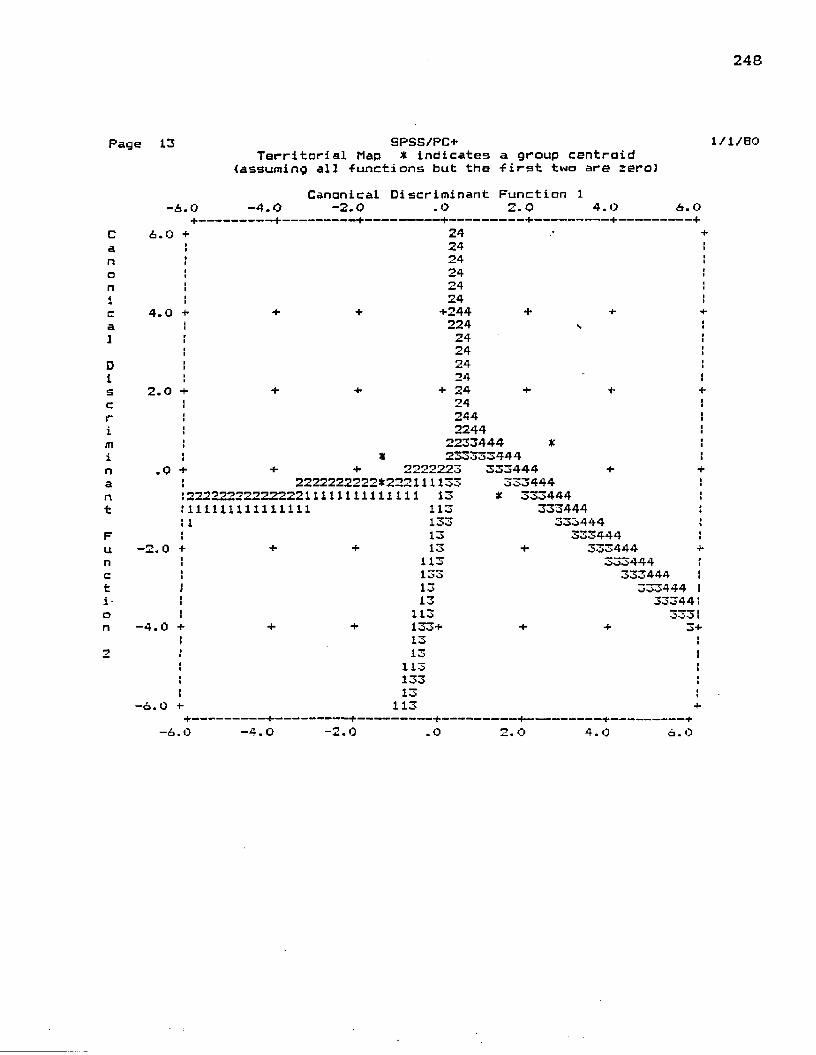
248

Page 13 SPSS/PC+Territorial Map * indicates a group centroid

{assuming all functions but the first two are zero)

cananica1Di5CriminantFu n c t i ■ o n

- 6.0 -4.0Canoni cal

- 2.0Di scr inunant

.OFunction2.0 ,0

- + -,0- +

6.0 +

4.0

2.0

.0

- 2.0

-4.0

+ 22222232222222222*222111133

2 2 2 2 2 2 2 2 2 2 2 2 2 2 1 1 1 1 1 1 1 1 1 1 1 1 1 1 1 1 1 1 1 1 1 1 1 1 1 1 1 1 11

- 6.0 +

13 113 133 13 13

113 133 13 13

113 133+ 13 13

113 133 13

113

242424242424

+244 +224 v24 24 24 24

+ 24 +24 244 2244

2233444 *2aoo a 44 4

333444 3 3 3 4 4 4

* 333444333444

333444 333444

00^444 333444

ooo444 333444

33344 333

+ 3+

-6+ -

,0 -4. O i. 0 2.0 4.0 6.0

i / i /e o

249

Page 20

Cananica1DiscriminantFUnction

OutX-

Out Xiii

SPSS/PC+All—groups Scatterplat — * indicates a group centroid

Canonical Discriminant Function 1 -4.0 -2.0 .0 2.0 4.0

1/1/SO

4.0

2.0 +

.0 +I

- 2.0 +

-4.0

Out-XX

t-t-2 1 212

2242

2 2 22 * 421 2 1 2 4 421* 2 4 2

2 313 33 *111 2 32 4 33

1 3 32 2 1 311

4 4* 44 3 +I

33 3

Out XX-

Out -4.0 -2. 0 . 0 2.0 4. 0X

-XOut

itDn

ijfa

H-in

uH’O

d n

250

Page 21GroupOut

X-Out X

-4. 0

can0 n.1 4.0 + I

2.0

.0

- 2.0uncti□n

-4.0

SPS5/PC+ 1/1/80female attender * indicates a group centroidCanonical Discriminant Function 1

-2.0 .0 2.0 4.0 Out-------- +---------- +---------- +----;----- +---------- X

XIIt

11litill

Out X

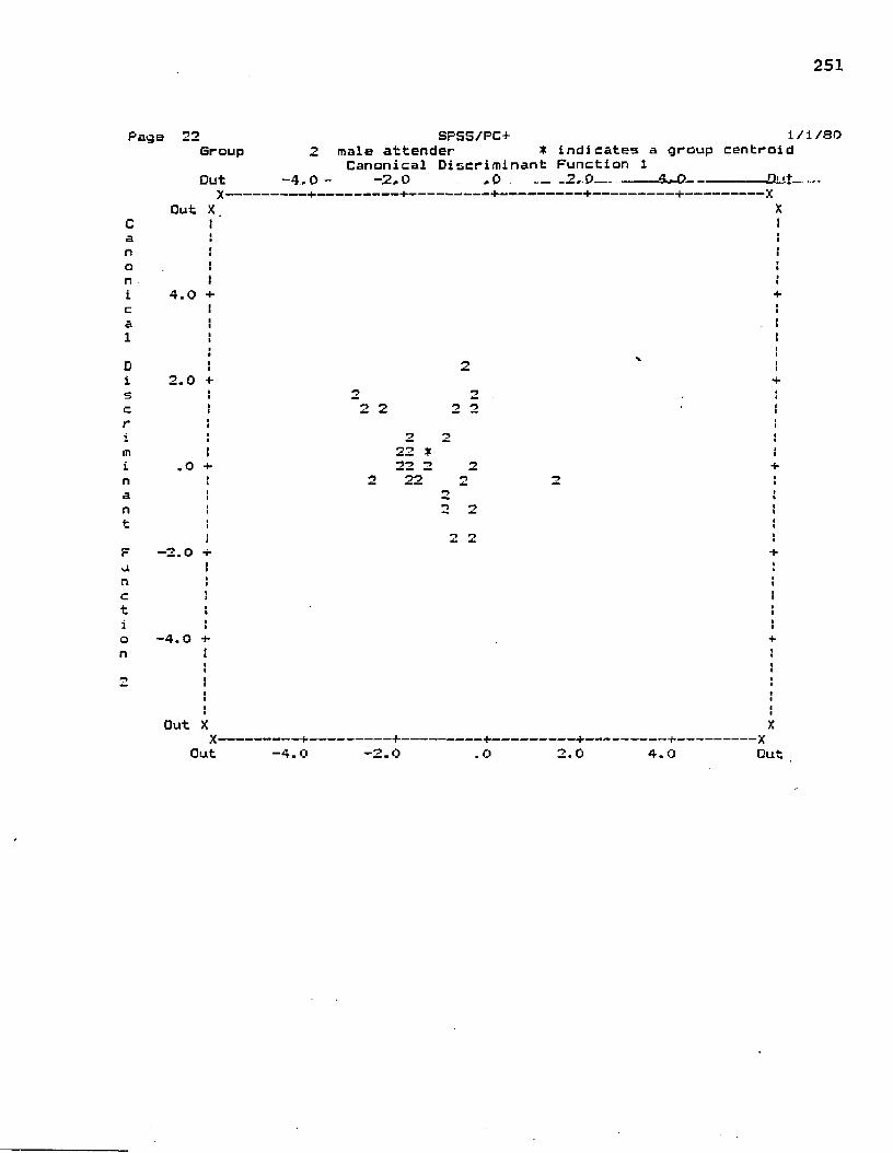
251

Page

Cananica1

GroupOut

X-Out X

-4

SPSS/PC+2 male attender * indicates

Canonical Discriminant Function 1 , 0 - -2, D ,0 ----2,0-------

1/1/80 a group centroidJk O- -Uiif-..--------- +---------- +---------- +---------- +---------- X

4.0 +

Di3Criminant

2.0 +2 2 2 2

2 2 22 *22 2 2

2 22 2 2

Function

- 2.0

-4.0

Out XX--

Out -4.0 + -

-2. 0 .0 2.0 4.0X

-XOut

252

Page 23 SPSS/PC+ 1/1/SOGroup 3 -female nonattender * indicates a group centroid

Canonical Discriminant Function 1 -4.0 -2.0 .0 2.0 4.0 Out

Can□nica1DiscriminantFunction

OutX-

Cut X

4.0 +

2.0 +■

- 2.0 +

-4.0 +

3 3 33 4 333

S 3 3

iOut X

X-Out -4.0 -2.0 2. 0 4.0

X-XOut

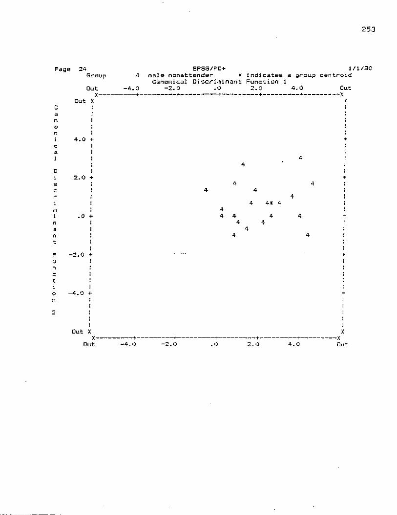
253

Page 24GroupOut

X-□ut X

ItI

4.0 +

-4. 0

SPSS/PC+ 1/1/SOmale nonattender * indicates a group centroidCanonical Discriminant Function 1

-2.0 .0 2.0 4.0 Out

2.0 +

.0 +44 4

- 2.0 +

ncton

-4.0 -t*

4 4* 44 4

Out XX’Out -4.0

+ .

- 2.0X

-XG u t2. O 4. 0

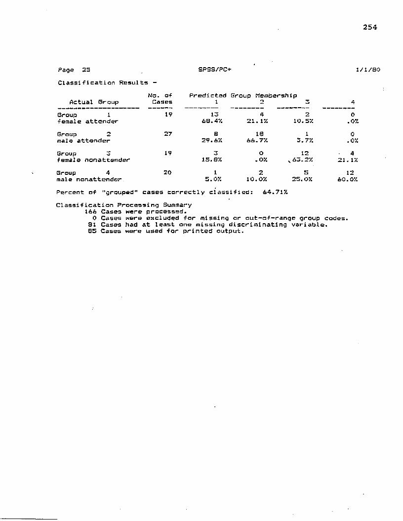
254

Page 25Classification Results -

Actual GroupGroup 1female attenderGroup 2male attenderGroup 3female nonattenderGroup 4male nonattender

No. of Cases

19

27

19

20

SPS5/PC+

Predicted Group Membership 1 2

1/1/80

13 68. 47.

829.67.

315.8%

15.0%

421. 1%

1866.77.

0.0%n

10.0%

210. 5%

13.7%12

„63.2%5

25. 0%

0.0%0.07.4

21. 1%12

60.0%Percent of "grouped" cases correctly classified: 64.71%Classification Processing Summary

166 Cases were processed.0 Cases were excluded for missing or out-of-range group codes.

81 Cases had at least one missing discriminating variable.95 Cases were used for printed output.

APPENDIX NMULTIVARIATE ANALYSIS OP VARIANCE ON STUDENT SATISFACTION AND GRADE POINT AVERAGE BY GROUP ASSIGNMENT ON NINTH GRADE DATA

255

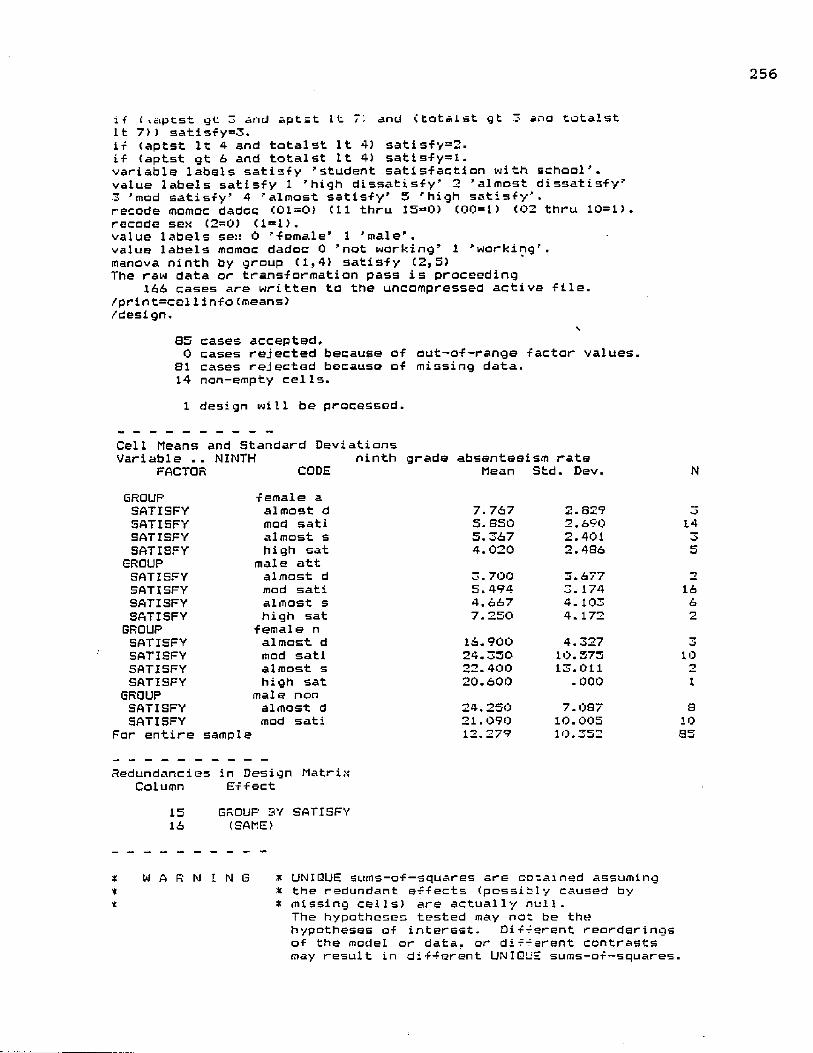
256

if ( iaptst gt 3 and sptst It and (totaist gt 3 ana tatalst It 7t) satisfy=3.if (aptst It 4 and tatalst It 4) satisfy=2. if (aptst gt 6 and totalst It 4) satisfy=I.variable labels satisfy 'student satisfaction with school', value labels satisfy 1 'high dissatisfy' 2 'almost dissatisfy'3 'mod satisfy’ 4 'almost satisfy’ 5 'high satisfy’.recode momoc dadoc (01=0) (11 thru 13=0) (00=1) (02 thru 10=1).recode sex (2=0) (1=1).value labels sex 0 'female' 1 'male'.value labels mamoc dadoc 0 'not working’ 1 'working', manova ninth by group (1,4) satisfy (2,3)The raw data or transformation pass is proceeding

166 cases are written to the uncompressed active file. /print=cellinfo(means)/design.

\S3 cases accepted.0 cases rejected because of out-of-range factor values.

SI cases rejected because of missing data.14 non-empty cells.1 design will be processed.

Cel 1 Means and Standard DeviationsVariable .. NINTH ninth grade absenteeism rate

FACTOR CODE Mean Std. Dev. NGROUP female aSATISFY almost d 7. 767 2. 829 3SATISFY mod sati 5. BS0 2.690 14SATISFY almost s 5.367 2.401 3SATISFY high sat 4.020 2.4B6 5

GROUP male attSATISFY almost d 3. 700 3.677 2SATISFY mod sati 5. 494 3. 174 16SATISFY almost s 4. 667 4. 103 6SATISFY high sat 7. 250 4. 172 2

GROUP female nSATISFY almost d 16.900 4.327 3SATISFY mod sati 24.350 10.575 10SATISFY almost s 22.400 13.011 2SATISFY high sat 20.600 .000 1

GROUP male nonSATISFY almost d 24.250 7.087 8SATISFY mod sati 21.090 10.005 10

"or entire sample 12.279 10.352 S3

Redundancies in Design MatrixColumn Effect

15 GROUP 3Y SATISFY16 (SAME)

* W A R N I N G * UNIQUE sums-of-squares are aocained assuming* * the redundant effects (possibly caused byt * missing cells) are actually null.

The hypotheses tested may not be the hypotheses of interest. Different reorderings of the model or data, or dif-arent contrasts may result in different UNIQUE sums-of—squares.

257

Page 2 SPSS/PC+* * ANALYSIS OF VARIANCE — DESIGN 1 * *Tests of Significance for NINTH using UNIQUE sums of squaresSource of Variation SS DF MS F Sig of FWITHIN CELLS 2378.14 71 40.54CONSTANT 771.67 1 771.67 19.04 .000GROUP 2476.15 3 825.38 20.36 . 000SATISFY 73.43 3 24.40 .60 * (3 1 kJGROUP BY SATISFY 209.S7 7 29.98 '.74 -639

1/1/30

8840 BYTES QF WORKSPACE NEEDED FOR MANDVA EXECUTION.

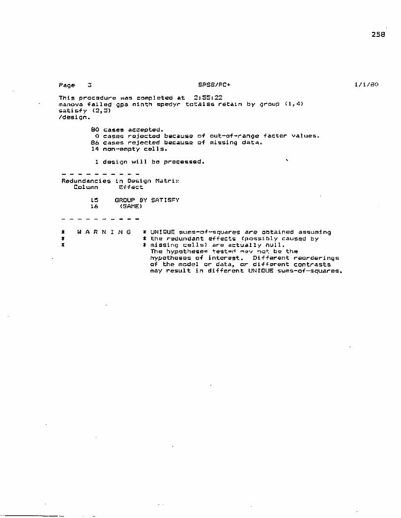
258

Page 3 SPS5/FC+This procedure was completed at 2:55:22manova failed gpa ninth spedyr totalss retain by group (1,41 satisfy (2,5)/design.

80 cases accepted.0 cases rejected because of out-of—range factor values.

86 cases rejected because of missing data.14 non-empty cells.1 design will be processed. v

Redundancies in Design Matrix Column Effect

15 GROUP BY SATISFY16 (SAME)

* W A R N I N G * UNIQUE sums—of—squares are obtained assuming* it the redundant effects (possibly caused byit t missing cells) are actually null.

The hypotheses tested mav not be the hypotheses of interest. Different reorderings of the model or data, or different contrasts may result in different UNIQUE sums—of—squares.

1/1/80

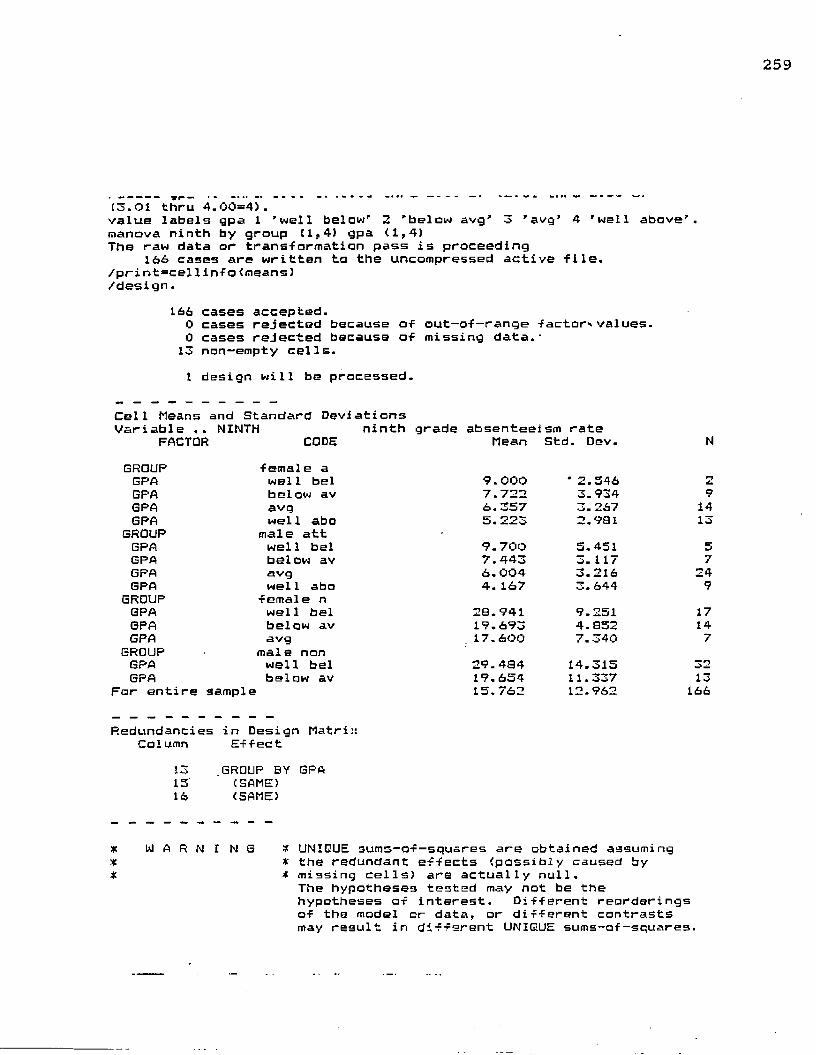
(3.01 thru 4.00=4).value labels gpa 1 'well below' 2 'below avg' 3 ’avg’ 4 'well above', manova ninth by group (1,4) gpa (1,4)The raw data or trans-formation pass is proceeding

166 cases are written to the uncompressed active file./pri nt=cel1 info(means)/design.

166 cases accepted.0 cases rejected because of out-of-range factor'values.0 cases rejected because of missing data.'13 non-empty cells.1 design will be processed.

Cell Means and Standard DeviationsVariable .. NINTH ninth grade absenteeism rate

FACTOR CODE Mean Std. Dev. NGROUP female aGPA well bel 9.000 * 2.546 2GPA below av 7.722 3.934 9GPA avg 6.357 3. 267 14GPA well abo 5.223 2.981 13

GROUP male attGPA well bel 9.700 5.451 5GPA below av 7.443 3. 117 7GPA avg 6.004 3.216 24GPA well abo 4. 167 3. 644 9

GROUP female nGPA wel1 bel 20.941 9.251 17GPA below av 19.693 4. 852 14GPA avg .17.600 7.340 7

GROUP male nonGPA well bel 29.484 14.315 32GPA below av 19.654 11.337 13

For entire sample 15.762 12.962 166

Redundancies in Design Matri::Column Effect

13 GROUP BY GPA 15' (SAME)16 (SAME)

* W A R N I N G * UNIGUE sums-of—squares are obtained assuming* * the redundant effects (possibly caused by* * missing cells) are actually null.

The hypotheses tested may not be the hypotheses of interest. Different reorderings of the model or data, or different contrasts may result in different UNIQUE sums—of—squares.

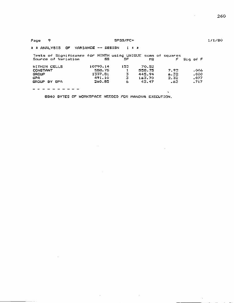
260

Page 9 SPSS/PC-*-* * ANALYSIS QF VARIANCE — DESIGN 1 * *Tests of Significance for NINTH using UNIQUE sums of squaresSource of Variation SS DF MS F Sig of FWITHIN CELLS 10790.14 153 70.52CONSTANT 558.75 1 558.75 7. 92 .006GROUP 1337.81 3 445.94 6. 32 .000GPA 491.10 3 163.70 2. 32 .077GROUP BY GPA 260.85 6 43.47 .62 .717

8940 BYTES OF WORKSPACE NEEDED FOR MANOVA EXECUTION.

1/ 1/80

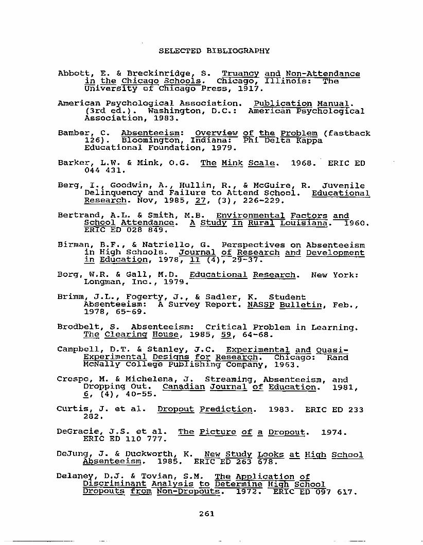
SELECTED BIBLIOGRAPHY

Abbott, E. & Breckinridge, S. Truancy and Non-Attendance in the Chicago Schools. Chicago, Illinois: TheUniversity of Chicago Press, 1917.American Psychological Association. Publication Manual.(3rd ed.). Washington, D.C.: American PsychologicalAssociation, 1983.Bamber, C. Absenteeism: Overview of the Problem (fastback126}. Bloomington, Indiana: pEi Delta KappaEducational Foundation, 1979.Barker, L.W. & Mink, O.G. The Mink Scale. 1968. ERIC ED 044 431.Berg, I., Goodwin, A., Hullin, R., & McGuire, R. Juvenile Delinquency and Failure to Attend School. Educational Research. Nov, 1985, 27, (3), 226-229.Bertrand, A.L. & Smith, M.B. Environmental Factors andSchool Attendance. A Study in Rural Louisiana. 1960. ERIC ED 028 849.Birman, B.F., & Natriello, G. Perspectives on Absenteeism in High Schools. Journal of Research and Development in Education. 1978, 11 (4), 29-37.Borg, W.R. & Gall, M.D. Educational Research. New York: Longman, Inc., 1979.Brimm, J.L., Fogerty, J., & Sadler, K. StudentAbsenteeism: A Survey Report. NASSP Bulletin, Feb.,1978, 65-69.Brodbelt, S. Absenteeism: Critical Problem in Learning.The Clearing House. 1985, 59, 64-68.Campbell, D.T. & Stanley, J.C. Experimental and Quasi- Experimental Designs for Research. Chicago: RandMcNally College Publishing Company, 1963.Crespo, M. & Michelena, J. Streaming, Absenteeism, andDropping Out. Canadian Journal of Education. 1981.6, (4), 40-55.Curtis, J. et al. Dropout Prediction. 1983. ERIC ED 233 282.DeGracie, J.S. et al. The Picture of a Dropout. 1974.ERIC ED 110 777.DeJung, J. & Duckworth, K. New Study Looks at High School Absenteeism. 1985. ERIC ED 263 678.Delaney, D.J. & Tovian, S.M. The Application ofDiscriminant Analysis to Determine High School Dropouts from Non-Dropouts. 1972. ERIC ED 097 617.

261

262

Dictionary of Occupational Titles. (1977). Washington, DC: U.S. Government Printing Office.Dudley, G.O. Report of Indiana Public School Dropout-Graduate Prediction Study. 1971. ERIC ED 062 666.Eaton, M.J. A Study of some Factors Associated with the Early Identification of Persistent Absenteeism. Educational Review, 1979, 31 (3) , 233-241.Erickson, E. et al. Final Report of the Evaluation of the 1970-71 School-Home Contact Proqram. New York State Urban Education. 1971. ERIC ED 064 423.Fiordaliso, R. et al. Decreasing Absenteeism on the Junior High Level. 1976. ERIC ED 123 764.Fiordaliso, R., Lordeman, A., Filipczak, J., & Friedman,R.M. Effects of Feedback on Absenteeism in the Junior Hiqh School. The Journal of Educational Research, 1977, 70, 188-192.Fogelman, K. School Attendance, Attainment, and Behavior. British Journal of Educational Psvcholoqy, 1978,48, 148-158.Fox, W.M. & Elder, N. A Study of Practices and Policies for Discipline and Dropouts in Ten Selected Schools. 1980. ERIC ED 191 974.Galloway, D. Size of School, Socio-Economic Hardship,Suspension Rates, and Persistent Unjustified Absence from School. British Journal of Educational Psychology, 1976, 46, 40-47.Green, D.A. A Study of the Relationships Between School Persistence and Grades, Ability and Achievement of Secondary School Pupils. Unpublished doctoral dissertation (microf.), State University of Iowa,1958.Heffrez, J. Employment and the High School Dropout. NASSP Bulletin, Nov., 1980, 85-90.Hersov, L., & Berg, I. Out of School: Modern Perspectives on Truancy & School Refusal Chichester, New York, Brisbane, Toronto: John Wiley & Sons LTD., 1980.Kerlinger, F. N, Foundations of Behavioral Research. New York: Holt, Rinehart, and Winston, Inc., 1973.Kerlinger, F.N. Multiple Regression in BehavioralResearch. New York: Holt, RineKart, and Winston,Inc., 1973.Klecka, W.R. Discriminant Analysis. Beverly Hills, California: SAGE Publications, Inc., 1980.

263

Krathwohl, D.R. How to Prepare a Research Proposal.Syracuse, New York: Syracuse University Bookstore,1973.Lutz, G.M. Understanding Social Statistics.„ New York: MacMillan Publishing Co., Inc., 1983.Nachman, L.R., Getson, R.F., & Odgers, J.G. Ohio Study of High School Dropouts 1962-1963. 1964. ERIC ED 029

Nagle, R.J., Greshman, F.M. & Johnson, G. Truancy Intervention Among Secondary Special Education Students. School Psychology Digest, 1979, 8 (4), 464- 468.Neill, S.B. Keeping Students in School: Problems andSolutions. AASA Critical Issues Report. 1979. ERIC ED 177 704.Neyman, C.A. Jr. Analysis of the Methods Used forIdentifying Potential School Dropouts. Final Report. 1969. ERIC ED 059 249.Nie, N.H., Hull, C.H., Jenkins, J.G., Steinbrenner, K. & Bent, D. H. Statistical Package for the Social Sciences (2nd ed.). New York: McGraw-Hill BookCompany, 1970.Norusis, M.J. SPSS/PC+ For The IBM PC/XT/AT. Chicago, Illinois: SPSS, Inc., 1986.Oakland Schools7 Testing Handbook 1985-86. Pontiac, Michigan: Oakland Schools, 1985.Operation DIRE (Dropout Identification, Rehabilitation, and Education), A Report of the Study and Findings. 1966.ERIC ED 036 938.Orange County Dropout Prediction Study. 1965. ERIC ED 075 729.Penty, R.C. Reading Ability and High School Dropouts. New York: Bureau of Publications, Teachers College,Columbia university, 1956.Rodell, D. E. Taking a Ride on a Merry-Go-Round: AnAttempt at Systems Change in a Public School. The High School Journal, Mar., 1979, 257-262.Schrora, L.K. Factors Influencing Year 9 Students7Intentions to Leave School. 1980. ERIC ED 209 484.Secondary School Dropouts. Minnesota State Department of Education, St. Paul. 1981. ERIC ED 205 684,Self, T.C. Dropouts: A Review of the Literature. ProiectTalent Search. 1985. ERIC ED 260 307.

264

Smith, J.E., Tseng, M.S., & Mink, O.G. Prediction of School Dropouts in Appalachia: Validation of a Dropout Scale. Measurement and Evaluation in Guidance. 1971, 4 (1), 31-36.Snepp, D.W. Can We Salvage the Dropouts? The Clearing House, Sept., 1956, 49-54.Snowbarger, V.A. Factors Associated with Truancy Among Boys in Selected Junior High Schools of Los Angeles County. Unpublished doctoral dissertation (microf.), the University of Southern California, 1954.Spencer, E.C. An Analysis of the Dropout in Norfolk Secondary Schools. 1977. ERIC ED 151 461.Tatsouka, M.M. Discriminant Analysis: The Study of GroupDifferences" Champaign, Illinois: Institute forPersonality and Ability Testing, 1970.Tennent, T.G. School Non-Attendance and Delinquency. Educational Research, 1974, 62 (16), 185-189.Timberlake, C. Why Do Students Drop Out of School? A Selected and ReTated Literature Review. 1980.ERIC ED 189 502.Turabian, K.L. A Manual for Writers (5th ed.). Chicago, Illinois: The University of Chicago Press, 1987.Varner, S.E. School Dropouts. 1967. ERIC ED 025 017.Vocational Education Early School Leaver Study. Final Report. 1978. ERIC ED 164 987.Vultaggio, D. "Student Absenteeism in the SecondarySchools", an unpublished paper for a school district within Oakland County, Michigan, 1984.Walberg, H.J. Improving the Productivity of America'sSchools. Educational Leadership. May, 1984, 19-27.White, R. Absent with Cause: Lessons of Truancy.London, Boston, and Henley: RoutlecTge & Kegan PaulLTD., 1980.Wilson, A. Jr. Development and Implementation of aStructural Program for the Systematic Reduction of Factors Contributing to Students Dropping Out of School. 1977. ERIC ED 154 268.Yaffe, E. More Sacred than Motherhood. Phi Delta Kappan, Mar., 1982, 469-470.Young, V. & Reich, C. Patterns of Dropping Out. Toronto Board of Education Research Service NumEer 129.1974. ERIC ED 106 720.

ABSTRACT

ADOLESCENT BEHAVIOR: VARIABLES AFFECTING SCHOOL ATTENDANCEby

NANCY KAY OWENS December, 1988

Advisor: Donald R. Marcotte, Ph.D.Major: EVALUATION AND RESEARCHDegree: DOCTOR OF PHILOSOPHY

The purpose of the research was to determine whether group differences by gender occurred between students who attended school and students who did not attend school on a regular basis at the twelfth grade level and whether those differences were similar for a second sample of ninth grade students. The general objective of the study was to develop a profile of a suburban school district non- attender by utilizing student data readily accessible from school records. Several variables were used in the study based upon an analysis of previous studies discussed in the literature review.

The research involved identifying those variables that could collectively contribute in distinguishing non- attenders from attenders. Discriminant analysis procedures showed that the strongest contributions in discriminating among the groups at both grade levels was language achievement, grade point average, and current grade level absence rates. Male non-attenders' performance on language related test items on the Comprehensive Test of Basic Skills was significantly lower when compared to the female non-attenders' performance as well as the other attenders'

265

266

groups. In addition, the male non-attenders failed almost twice as many classes as the female non-attenders. Approximately 62 percent of the twelfth grade students were correctly classified; whereas, 65 percent were properly classified at the ninth grade level.

A limitation of the study centered on the loss of cases in the discriminant analysis procedure due to students having missing data on at least one of the several independent variables. The most frequent data that were missing were test scores.

It was recommended that the subject suburban school district or any other school district possessing similar characteristics identify poor performers in language- related activities at an early age along with students who exhibit at least a five percent absence rate and then address those deficiencies prior to the students attending junior high school.

Further research was suggested in the area of language achievement by identifying specific skill deficiencies or by examining the effects of an experimental language arts program on student absenteeism rates when compared to a traditional language arts program at the junior high or middle school level. Also, future research endeavors in the area of student satisfaction with school as it relates to academic achievement and aptitude with student absenteeism rates could be analyzed at an earlier age level with or without regard to gender.

AUTOBIOGRAPHICAL STATEMENT

Name:

Born:

Education:

ProfessionalBackground:

Professional Memberships:

NANCY KAY OWENS

July 1, 1951 Saginaw, Michigan

Delta Community College, Saginaw, MichiganWestern Michigan University, Kalamazoo, MichiganBachelor of Arts, 1972Oakland University, Rochester, Michigan Master of Arts in Teaching, 1973Wayne State University, Detroit, Michigan Doctor of Philosophy in Educational Evaluation and Research, 1988

Secondary Reading TeacherWaterford Mott High School 1973-1978Alternative Education Consultant Waterford School District 1978-1981Pupil Accountant & Program Evaluator Waterford School District 1981-1985Statistical AnalystGeneral Motors Inland DivisionLivonia Plant 1985-1986Supervisor of Training ProgramsGM Inland Division - Livonia 1986-1987Supervisor of UAW-GM Joint Programs GM Inland Division - Livonia 1987-Present

Michigan Educational Research Association Michigan Pupil Personnel Administrators Association Institute for Industrial Engineers International Association for Personnel Women

267