† We thank Sudheer Chava, Vikram Nanda, Qinghai Wang, and seminar participants at Georgia Tech. We are grateful to Jay Ritter for providing data on Institutional Investor All-Star analysts. Any remaining inadequacies are ours alone. Clarke is at the College of Management, Georgia Institute of Technology: jonthan.clarke@mgt.gatech.edum, (404) 894-4929. Ornthanalai is at the College of Management, Georgia Institute of Technology: chay.ornthanalai@mgt.gatech.edu, (404) 385-4569. Tang is at the Guanghua School of Management, Peking University: yatang@gsm.pku.edu.cn, (86)-10-627-67568.

Informational Herding by Institutional Investors: Evidence from Analyst Recommendations

Jonathan Clarke, Chayawat Ornthanalai, Ya Tang† Georgia Institute of Technology and Peking University

This version: November, 2010

Abstract

We study daily institutional herding levels around the release of sell-side analyst recommendations. Such recommendations are forward-looking and indicate unambiguous direction of trades thus providing a good scenario to investigate informational herding behavior. We find that institutional herding on the recommendation release date is short-lived and specific to high turnover stocks suggesting that institutional investors herd during periods of significant disagreement. We do not find that institutional herding around recommendations destabilizes prices, but rather herding helps to speed up the information incorporated into stock prices. Consistent with investigative herding models, our results suggest that institutional investors herd upon the arrival of correlated information signals, and that such action improves market efficiency. This is in clear contrast with non-informational herding models, which are associated with subsequent return reversals.

Keywords: Institutional trading, herding, market efficiency, analysts’ recommendations

1  

1. Introduction

Theoretical herding models provide two main hypotheses regarding the price effect of herding. In

information-based herding models, such as Froot, Scharfstein, and Stein (1992) and Hirshleifer,

Subrahmanyam, and Titman (1994), herding can facilitate market efficiency by quickly impounding

information into asset prices. Alternatively, when investors herd because of non-informational

reasons, such as the reputational risk of acting differently than others (Scharfstein and Stein (1990)),

behavioral instincts (see Friedman (1984), Dreman (1979), and Barberis and Shleifer (2003)), or the

non-risk based preferences towards certain security characteristics (Falkenstein (1996)), herding can

destabilize prices away from intrinsic value, resulting in subsequent return reversals.

The question of whether institutional herding has a stabilizing or destabilizing influence on

stock prices has been the focus of a large number of recent empirical studies. Answering this

question is crucial for regulatory purposes, because if institutional herding has a destabilizing effect,

price reversals may occur and threaten the stability of financial markets. Unfortunately, the evidence

regarding the price effect of institutional herding is decidedly mixed. Some studies document

subsequent return reversals following institutional herding and conclude that herding moves prices

away from their fundamental values (e.g., Brown, Wei and Wermers (2010), Dasgupta, Prat, and

Verardo (2010), Gutierrez and Kelley (2009), Puckett and Yan (2010), and Christoffersen and Tang

(2010)). Other studies detect return continuation following institutional herding and conclude that

correlated institutional trades aid in the price discovery process and help improve market efficiency

(e.g., Grinblatt, Titman and Wermers (1995), Nofsinger and Sias (1999), Wermers (1999), Sias

(2004)).

We argue that one of the primary reasons for the mixed findings on the price impact of

institutional herding is that most previous studies do not distinguish between informational herding

and non-informational herding. Therefore, the real price effect of herding may be hidden by the

2  

averaging of results across the various reasons to herd.

The purpose of this study is to investigate informational herding (or “investigative herding”)

by institutional investors around the release of analyst recommendations and examine its impact on

stock prices at the daily level. Investigative herding arises when investors trade similarly by reacting

to the arrival of a commonly observed information signal. There are a number of reasons why

analysts’ recommendation releases are suitable for the study of informational herding. First, analysts’

recommendations have been shown to influence the trading of institutional investors.1 Second,

analyst recommendations, unlike other commonly studied public news releases such as earning

announcements and management guidance, give an unambiguous signal on the direction of trades.

Third, analyst’s recommendations are forward-looking opinions based on the analyst’s private

information rather than evidences of past performance such as earnings announcements.

Another important aspect that discerns our work from most previous studies is that we

focus on the daily institutional herding level rather than at the quarterly horizon. We argue that it is

important to study the price impact of institutional herding over short horizons because if the price

destabilization effect were to be an outcome of such action, it is most likely to appear in the short-

run. This is because in a well-functioned market, price movement associated with correlated large

trades is more likely to be absorbed by the market and dissipates overtime. Furthermore, as

suggested by Puckett and Yan (2010), limits to arbitrage such as short-sale constraints are more

binding in the short-term, thus price deviations from the fundamental values are more likely to be

arbitraged way over a long horizon.

Our primary results are as follows. First, we show that institutions herd on the

recommendations of analysts. To ensure that our results are not contaminated by other confounding

                                                            1 See for examples, Chen and Cheng (2006), Kacperczyk and Seru (2007), Mikhail, Walther and Willis (2007), and Busse, Green and Jagedeesh (2008))

3  

news, we remove recommendations that are issued within +/- 10 days of earnings announcements

and management guidance releases. Using trades and quotes data over the period from 1995 to

2006, we construct a measure of daily abnormal herding and find that abnormal buy (sell) herding is

2.18% (-2.51%) around the releases of upgrades (downgrades). The abnormal herding occurs only

on the recommendation release date and the effect is stronger for recommendation downgrades

than for upgrades.

A recent study by Brown, Wei and Wermers (2010) uses quarterly institutional holding data

and quarterly data on consensus analyst recommendations to document mutual funds herding -into

stocks receiving a consensus upgrade and herd out of stocks receiving a consensus downgrade. In

contrast to Brown, Wei and Wermers (2010), we examine herding at the daily level and herding

around individual analyst recommendations rather than consensus forecasts. These two extensions

are important because herding is a short-lived phenomenon, and hence, may be difficult to detect

cleanly in a long horizon study (e.g., Banerjee (1992), Bikchandani, Hirshleifer, and Welch (1992),

Avery and Zemsky (1998)). Moreover, individual analyst recommendations provide an information

event to directly test the existence and the influence of informational herding.

We also document evidence that institutional investors herd on analyst recommendations

when investor disagreement is large. Consistent with the differences of opinion literature (see, e.g.,

Kim and Verrecchia (1994), Bamber, Barron and Stober (1997, 1999), Kandel and Pearson (1995),

and Banerjee and Kremer (2010)), we find that shares turnover increases tremendously prior to the

analyst recommendations, reflecting a large jump in disagreement in the market. Correspondingly,

we find that institutional herding around analyst recommendations is pronounced only when shares

turnover is high. This result stands in sharp contrast to previous studies which investigate the overall

herding level in financial markets rather than those that are driven by an information event: the level

4  

of herding, overall, is stronger for small-size and low-turnover stocks. Our opposite finding on the

relationship between institutional herding level and shares turnover suggest that informational

herding is fundamentally different from the overall herding behavior which may be due to other

externalities, such as information asymmetry or reputation concern.

We also examine how the level of institutional herding on analyst recommendations is

related to characteristics of the recommendation sources. Consistent with investigative herding

theory that investors are more likely to behave similarly in response to more credible information

signal, we find some evidence that herding is related to proxies for the reputation of analysts. More

precisely, we find that institutional investors sell-herd more around the downgrades that are issued

by all-star analysts.

We then examine the impact of institutional herding on the abnormal returns surrounding

recommendation changes. When herding is in the direction of the recommendation (i.e., sell herding

around a downgrade), we find that institutional herding speeds the price adjustment process. This

finding is consistent with Wermers (1999) and the broader literature on investigative herding

models. Futhermore, we find that when recommendation upgrades (downgrades) are accompanied

by strong institutional buy (sell) herding, the bulk of price adjustment occurs on the

recommendation release date and that post-recommendations returns are generally insignificant. We

find a number of cases where a recommendation change is accompanied by strong contrarian

herding. Contrarian herding occurs when a recommendation downgrade (upgrade) is accompanied

by strong abnormal buy (sell herding). In these instances, we find evidence of return reversals.

Recommendation downgrades accompanied by strong buy herding initially generate a positive and

significant announcement period return. However, this positive return reverses over the next 2 to

10 business days. We find a similar result for recommendation upgrades accompanied by strong sell

5  

herding. These results suggest that institutional herding in the direction of a recommendation

change promotes price discovery, while intense contrarian trading against recommendations blocks

new information from being incorporated into stock prices.

While we do not find evidence of return reversals when a recommendation change is

accompanied by institutional herding in the same direction, we find evidence of subsequent return

reversals when looking at the overall institutional herding behavior in financial markets. Specifically,

we form daily portfolios over 1995-2006 based on the top quintile of institutional buy and sell

herding levels and find subsequent return reversals within a week after the portfolio formation date.

This finding is highly consistent with Puckett and Yan (2010) who use Abel Noser institutional

trades data, and Christoffersen and Tang (2010), who use TAQ data, to study the price effect of

short-term institutional herding.2 Besides reconciling our results with the existing literature, this final

exercise highlights the importance of studying informational herding separately from herding that is

motivated by non-informational reasons.

In summary, our study contributes to two strands of literature. The first is the short-term

institutional herding literature. To the best of our knowledge, we are the first to investigate herding

in response to an information event using high-frequency trading data. We specifically examine how

traders react to analyst recommendations and link the evidence of institutional herding around

analyst recommendations with models of investigative herding. Second, our study contributes to the

literature on the information intermediary’ role of analysts. Our results show that security analysts

play an important role in facilitating beliefs convergence among institutional investors and that their

                                                            2 Alternatively, we can measure institutional herding at the weekly level as in Puckett and Yan (201) using the Abel Noser data. However, such method would not permit us to study institutional herding on individual analyst recommendations. Besides, our findings are based on the full universe of stocks rather than a subset of trades within a consultancy group which makes up the Abel Noser data.

6  

influence is stronger during periods of large investor disagreement. Contrary to Altinkilic and

Hansen (2009, 2010), our results suggest that analysts are important information intermediaries.

The remainder of this paper proceeds as follows. Section II discusses related studies and our

hypotheses. Section III discusses our data and methods. Section IV presents our empirical findings,

while Section V offers our concluding comments.

2. Background and hypotheses development

Prior studies have argued that rational herd behavior and informationally efficient asset prices are

not mutually exclusive (Bikchandani and Sharma (2005) and Devenow and Welch (1996)).

Informational herding, or investigative herding, indicates a situation in which the investors trade

similarly in responding to a correlated information signal. Thus, investors can profit from the

information because it has been observed by others and subsequently reflected in the price.

Intuitively, “investigative herding” could arise when an information event occurs and investors act

upon the arrival of the commonly observed information signal. As a consequence of investigative

herding, we expect trades to be highly correlated and to quickly impound information conveyed by

an event.

We focus on analyst recommendations because they are known to carry useful predictive

information about stock values and sophisticated investors are likely to account for the information

conveyed in the recommendations in their trading. More importantly, unlike other commonly

studied public news, recommendation upgrades and downgrades give an unambiguous signal on the

direction of trades.

We first investigate whether institutional investors herd on analyst recommendations. In a

related study, Brown, Wei and Wermers (2010) find evidence that mutual fund managers herd into

7  

stocks with consensus upgrades and herd out of stocks with consensus downgrades based on

quarterly institutional holding data. However, changes in institutional holdings at the quarterly level

are more likely to reflect information gathered over the quarter rather than the information

contained in analyst recommendations; and the consensus of analyst recommendations prevents one

from making conclusive statements about whether institutional investors follow individual analyst

recommendations. We address the above issues by testing whether institutional investors tend to

trade excessively in the direction of the individual analyst recommendation. In addition, favorable

recommendations (upgrades) are known to be less credible and less lucrative than unfavorable

recommendations (downgrades), because prior studies show that analysts are reluctant to issue

negative recommendations for the companies they cover. Therefore, we would expect institutional

trading to be more sensitive to downgrades than to upgrades. This leads to our first hypothesis:

Hypothesis 1 (H1): Abnormal institutional buy (sell) herding is expected around the announcement of upgrades

(downgrades). Abnormal sell herding following downgrades is expected to be stronger than abnormal buy herding

following upgrades.

In a well-functioning market, herding should be fragile: the stock price adjusts quickly upward

(downward) to reflect the institutional buy (sell) herding. Additionally, existing studies indicate that

the investment value of analyst recommendation is short-lived. For instance, Dimson and Marsh

(1984) and Brennan, Jegadeesh, and Swaminathan (1993) find that the price adjustment to analyst

recommendations is very quick, while Barber, Lehavy, McNichols and Trueman (2001) document

evidence that the profit from purchasing (selling short) stocks with favorable (unfavorable)

consensus recommendations decreases over the portfolio rebalancing windows. There are two

implications from the above arguments: first, institutional investors need to react quickly in

8  

capitalizing the information conveyed in the analyst revisions; second, this revision-induced trading

by a herd cannot last over long periods of time. Therefore, our second hypothesis considers the

fragility of the observed herding

Hypothesis 2 (H2): Abnormal institutional herding around analyst recommendation revisions is expected to be short-

lived.

In the following set of predictions, we focus on the conditions for which institutional investors are

more likely to herd on analyst recommendations. If institutional trades cluster on the same side of

the analyst recommendations because investors react to the positively correlated signals or face a

similar information set, they are more likely to herd when they believe that the quality of the

information signal is high. Prior studies indicate that all-star analysts are believed to issue more

credible recommendations due to their superior information. Therefore, we expect the level of

institutional herding around analyst revision to be positively related with the analyst’s reputation. In

addition, Trueman (1994) and Welch (2000) provide evidence that security analysts also herd

following the prevailing consensus. We thus expect institutional investors to discount

recommendations that simply confirm previous recommendations because such recommendations

are redundant and do not contain credible new information. On the other hand, we would expect

institutional investors to react more strongly to those recommendations that are innovative (i.e.,

away from the consensus).

There is a growing literature that public news release is always associated with a jump in

heterogeneity or disagreement.3 When investors’ opinions increasingly diverge, informed investors’

investment decisions are more likely to be influenced by the arrival of an unambiguous information                                                             3 See Kim and Verrecchia (1994), Bamber, Barron and Stober (1997, 1999), and Kandel and Pearson (1995).

9  

signal, i.e. analyst recommendations. The above arguments lead to two predictions for our third

hypothesis:

Hypothesis 3:

(H3_a): Institutional investors are expected to react more strongly to recommendation revisions that are perceived to be

more credible.

(H3_b): Institutional investors are expected to herd more when there is higher disagreement in the market.

In the last hypothesis, we focus on whether institutional herding on analyst recommendations has a

stabilizing or destabilizing price effect. Even though the information is publicly announced, this

piece of value-relevant information does not arrive at all investors simultaneously but gradually flow

to whole market because of technology of information distribution or investor segmentation and

specialization ( e.g., Hong and Stein (1999), and Hong and Stein (2007)). The new information will

be gradually revealed and reflected in the asset price through the coordinating trading activities of

the market participants. That is, there is a positive information spillover when most investors trade

on the same side of the analyst recommendations (Froot, Scharfstein and Stein (1992), and

Hirshleifer, Subrahmanyam and Titman (1994)). Given the investment value of analyst

recommendations, the information-based herding around the recommendation releases would help

stock prices to more quickly reflect information in analyst revisions and improve market efficiency.

On the contrary, strong institutional trades against the analyst recommendations would block the

information incorporation into stock prices and induce price reversals. The above arguments lead to

our fourth hypothesis:

10  

Hypothesis 4 (H4): The magnitude of announcement period abnormal return is expected to increase with the intensity

of institutional herding on the recommendation release date. Price reversal is not expected in the post-recommendation

period if institutional investors herd in the direction of analyst revisions, while on the other hand, price reversal is

expected in the post-recommendation period if institutional investors herd against analyst revisions.

 

3. Data and Methods

3.1 Data

Analysts data

We obtain data on recommendation changes from the I/B/E/S database for the period between

1995 and 2006. For each recommendation, we obtain the recommendation level (1=strong buy,

5=strong sell), name of the analyst, name of the analyst’s employer, and the day and time of the

recommendation release. For recommendations issued after the market closes, we adjust the release

date to be equal to the next trading day. Time-stamped I/B/E/S recommendation data become

available in April 2009 and has been used in Bradley et al. (2010).

Panel A of Table 1 presents the frequency of recommendation upgrades and downgrades by

year. Overall, there are 49,909 recommendation changes between 1995 and 2006. Both the number

of upgrades and downgrades reached lows in 1995 and peaked in 2000. Consistent with existing

studies, we find more recommendation downgrades than upgrades. Roughly, 46% of

recommendation changes in our sample are upgrades, while the remaining 54% are downgrades.

Earnings announcement and management guidance data

Atlinklic and Hansen (2009), and Bradley et al. (2010) find that a substantial percentage of analyst

recommendations are released around corporate earnings news, most notably earnings

announcement and management guidance. In order to control for the impact of other corporate

11  

events, we collect time stamped earnings announcements data from I/B/E/S and management

guidance data from First Call. Similar to the procedure for recommendations, we adjust the date of

earnings announcement and management guidance that are issued after the market close to be equal

to the next trading day following their actual release date.

High frequency TAQ data

We calculate the daily herding level based on the intra-day trading data of NYSE stocks spanning the

period January 1995 to December 2006. Trades and quotes data are obtained from the TAQ data

set. To be included, a stock is required to (1) be listed on NYSE (ETN =1); (2) be a common stock

(TYPE = 0); (3) not be in the financial/real estate industry (ICODE >= 400); and (4) have records

on CRSP and I/B/E/S. Next, we purge the transaction data using the following filter rules: (1) we

only include the trades executed on the principle stock exchange, NYSE, to avoid the possibility of

the results being influenced by differences in trading protocols; (2) we only include trades and

quotes during normal trading time (9:30 am – 4:00 pm); (3) we exclude trades that have a special

settlement condition because they might be subject to distinct liquidity consideration; (4) we exclude

trades reported out of sequence, and quotes that do not correspond to normal trading

environments; (5) we exclude opening batch trades because the trading mechanism at the opening is

different from the rest of the day; (6) we exclude trades with prices larger than $999 or smaller than

$1, quotes where the bid or ask prices are larger than $999 or smaller than $1, and quotes with a

negative spread between bid and ask. Trades and quotes are separated in TAQ, each with its own

time stamp. In NYSE reporting procedure, quotes are updated after trades and hence trades are

reported late. To merge both data sets and rank their records chronologically, we apply the

12  

algorithm proposed by Lee and Ready (1991) to match the trade with the prevailing quote at 5

seconds prior to the trade.4

Categorizing trades

TAQ data does not provide information regarding the direction of the trade (buy/sell), nor does it

provide information about origin of the trade (institutional/retail). To address these problems, we

use two algorithms to help separate trades into buy/sell and retail/institutional categories.

First we use Lee and Ready’s (1991) algorithm to infer the trade direction. For trades which

are not at the mid-point of quoted spread, it is classified as buyer (seller)-initiated if the current trade

price is above (below) the quoted spread mid-point. For trades occurring exactly at the mid-spread,

a trade is classified as buyer (seller)-initiated if the sign of the last non-zero trade price change is

positive (negative). Alternatively, the quoted spread method and the tick-test-changes in trade price

method could be applied to classify trades. We obtain similar results using these methods.

Next, we classify institutional-based trades using Lee and Radhakrishna (2000) algorithm.

Institutional trades are identified as trades above $50,000, $20,000 and $5,000 for large firms,

medium firms, and small firms. After decimalization, the Lee and Radhakrishna (2000) algorithm of

separating trades is criticized because small trades may mix both institutional and retail trades, since

the institutions may break larger trades into several smaller ones. Campbell, Ramadorai, and

Schwartz (2009) develop a sophisticated cut-off rule and show that large trades classified using the

Lee and Radhakrishna (2000) algorithm are still associated with institutions. In this study, we focus

on large trades rather than small trades. Therefore, our results are not likely to be contaminated by

falsely classifying small trades as institutional ones. As a robustness check to address these concerns,

                                                            4 We also apply the 14 seconds matching rule proposed by Hasbrouck (1993) and the 2 second rule to reflect the fact that quotes are updated more frequently in recent years. Using these two methods produces similar results.

13  

we use both the Campbell, Ramodorai, and Schwartz (2009) and Lee and Radhakrishna (2000) cut-

offs to classify the trades and obtain similar results

3.2 Herding and abnormal herding

Herding Measure

We measure herding using the method developed by Lakonishok, Shleifer and Vishny (1992)

(hereafter LSV). The LSV measure is the most widely used statistical measure in the empirical

herding literature (e.g., Grinblatt et al.(1995), Wermers (1999), Chan et al. (2005)).

The herding formula for stock i on day T is defined as:

, , ∑ ,, (1)

where , represents the proportion of the number of buy-initiated trades for stock i in time

interval T and ∑ , is the cross-sectional average of , . The term , adjusts for the

expected excess proportion of buy-initiated trades under the null hypothesis that all trades are

independently transacted. 5 Essentially, equation (1) measures the tendency of traders to buy a

particular stock during the same period relative to the expected trading direction of traders that

make the investment decision independently.

Panel B of Table 1 summarizes the distribution of the daily LSV value, , , for all the

stocks in our sample. The median and the 10th and 90th percentiles of , show that the LSV

                                                            5Under the independent transaction null, the probability of any trader being a net buyer (seller) of stock (i) is p(t), the cross-sectional average fraction institutional buyer (seller) is p, then we can calculate

, ∑,

,,

where B is binomial variable with probability p and N(i,t) is the total number of trades for stock i in time period T.

14  

measure is generally positive. This finding is consistent with existing studies that use LSV method to

measure the herding level at different horizons (see Christoffersen and Tang (2010)).

Following Grinblatt et al (1995) and Wermers (1999), we use the “buy herding measure”

HB(i,T), and the “sell herding measure”, HS(i,T), to separate whether stock i has a higher (lower)

proportion of buyers than the average stock on day T. The formulas for these two conditional

herding measures for all trades are defined as:

, , , ∑ , (2)

i, T , , ∑ ,.

There are instances where we fail to identify trades as either institutional or retail. To make sure that

the LSV measure of herding is not distorted by infrequent trades, we drop an observation if there

are fewer than 20 institutional trades for a stock on a given day. Institutional buy-herding and sell-

herding are identified by HB and HS respectively. Each herding measure can be calculated over

different time intervals including intraday, daily, monthly and quarterly frequencies. In this paper, we

want to document the existence and the persistence of institutional herding around analyst

recommendations. While we could use shorter intervals, such as intraday, this could pose a problem

for infrequently traded small and medium size stocks. In order to maintain a large cross section of

firms in our sample and also maintain our focus on the short-term institutional herding level, we

compute the herding measure at the daily frequency.

In order to combine the buy- and sell-herding measures into a single variable, we follow the

method in Brown, Wei and Wermers (2010) and convert HB and HS into an adjusted herding

measure, , . The computation of the adjusted herding measure is as follows. For each day,

we find the minimum values of buy- and sell-herding values across all stocks. We then construct the

15  

adjusted buy (sell) herding measure HIB (HIS) by subtracting the daily minimum value of HB (HS)

from the buy (sell) herding measure of each stock. Consequently, the values of HIB and HIS are

always non-negative. The adjusted herding, , , is equal to HIB if the stock is a buy herding

stock and -1×HIS if the stock is a sell herding stock.

Panel B of Table 1 presents the distribution of the adjusted herding measure which appears

to be significantly left skewed. This finding is consistent with Brown, Wei and Wermers (2010),

which suggests that on average the aggregate level of herding in the market is on the sell side.

Abnormal Herding

Throughout the paper, we focus on the firm’s level of abnormal herding around sell-side

recommendations. Wermers (1999) provides evidence that the aggregate level of mutual fund

herding differs from one period to another. Furthermore, Acharya and Yorulmazer (2008) study a

theoretical model of bank herding and show that when banks loan returns have a common

systematic factor, they herd by undertaking correlated investments. In order to control for changes

in the firm’s herding level that is due to changes in the aggregate herding level in the market, we

estimate the following abnormal herding measure for firm j on day t:

, , , . (3)

The coefficients and are estimated from the following linear regression model:

, , , ,

where , is the equally weighted average value of , across all stocks on day t. The

coefficients and are estimated using a rolling window from t-35 days to t-6 days. This method is

similar in spirit to the market-model that is commonly used in the abnormal trading volume study

16  

(see Chae (2005) for an example). By construction, our measure of abnormal herding has a mean

near 0. For robustness, we also compute the abnormal herding measure using the value weighted

measure of the aggregate herding level and obtain the same results.

Abnormal Returns

We compute abnormal returns around analyst recommendations by implementing a two step

approach. In the first step, we estimate the Fama-French (1993) model augmented with Carhart’s

(1997) momentum factor over an estimation period that spans 255 trading days and ends on the 6th

trading day before the recommendation release. Specifically, the model is:

α β R s SMB h HML m UMD ε ,

where Rjt is the rate of return of the common stock of the jth firm on day t; Rmt is the rate of return

on the equally-weighted market portfolio on day t; SMBt is the difference in returns between a

portfolio of small and big stocks, HMLt is the difference in returns between a portfolio of high and

low book-to-market stocks, UMDt is Carhart’s (1997) momentum factor. In the next step, we use the

estimated coefficients for αj , βj , sj , hj, and mj to calculate abnormal returns each trading day over the

window (-1, +15), where day 0 corresponds to the recommendation release date.

Descriptive Statistics

In Panel B of Table 1, we present descriptive statistics for our herding measures, as well as, other

key variables. These descriptive statistics are generally consistent with previous studies. Firms in our

sample are large and actively traded, on average. The log of market capitalization averages 14.02,

average trading volume is 713,891 shares per day, and there are 155.62 trades per stock per day. Log

17  

turnover averages 1.15. The mean value for adjusted herding is -0.06, which is similar to the value

reported by Brown, Wei and Wermers (2010).

By design, the mean of abnormal herding is zero and this is evident in Panel B. The reported

descriptive statistics for and are the intercept and the slope of the estimation of abnormal

herding measure according to equation (3). We find that the estimates of are positive and

statistically significant for the majority of the firms and estimation periods. The aggregate herding

level therefore has a significant explanatory power on the herding level of a firm. This finding

emphasizes the importance of adjusting the firm-level herding for their co-variation with the

aggregate herding level in the event study analysis such as ours.

The average announcement period return for a recommendation upgrade is 1.76%, while a

recommendation downgrade generates an average announcement period return of -2.03%. The

significantly large abnormal return on the day of recommendation release is consistent with previous

studies such as Womack (1996).

The abnormal herding measure, , , that we introduce in this paper is designed to

remove the component in the firm-level herding that is due to changes in the level of herding.

Because , is a new measure, we study it in more details by examining whether its values

depend on the firms characteristics which have been have shown by other studies to explain the

herding level. Banerjee (1992), Bikhchandani, Hirshleifer and Welch (1992), and Avery and Zemsky

(1998) show that in an informational cascade model, herding behavior is more likely to occur among

stocks that have high uncertainty about the value of its asset. Prior studies show that the information

quality is relatively lower in small-sized firms and firms with low trading volume. Therefore, we

expect the institutional trades (herding) to be higher in smaller cap stocks and in those with lower

18  

shares turnover.6 The shares turnover variable is defined as the trading volume divided by the

number shares outstanding.

Table 2 summarizes the average value of abnormal herding measure by sorting them into

size and turnover quintiles. Consistent with the literature, we find that both institutional buy- and

sell-herding are stronger among small-cap stocks. We also find that abnormal sell-herding becomes

weaker as the turnover ratio increases. The relationship between abnormal buy-herding and turnover

quintiles is less clear.

We find that even after controlling for the aggregate herding level, the distribution of

abnormal herding is highly non-normal. In an unreported Kolmogorov test for normality, we

strongly reject the hypothesis that abnormal herding as well as standardized abnormal herding is

normally distributed. Consequently, we address the issue of non-normality in the event study

analysis of abnormal herding by focusing on the bootstrapped p-values when inferring the statistical

significance.

It is likely that the abnormal herding level is non-normal because its value depends on other

characteristics such as firm size, shares turnover, and bid-ask spread. Alternatively, we could include

an exhaustive list of potential determinants in equation (3). However, existing herding literature does

not provide guidance on how to estimate the abnormal herding level using multifactor models.

Therefore, we resort to a one-factor model for abnormal herding measure that accounts for changes

in the aggregate herding level. Nevertheless, when we examine the abnormal herding measure in a

regression framework, we include a series of control variables in the regression.

4. Results

                                                            6 Studies that document the firms’ information quality in a cross section include Brennan and Chordia (1993) and Grinblatt, Titman and Wermers (1995).

19  

4.1 Institutional herding surrounding recommendation release dates

Event study of abnormal herding

In this subsection, we test our first and second hypotheses by applying an event study framework to

the abnormal institutional herding measure, , . We first eliminate observations where either

an earnings announcements or management guidance occurs during the (-10, +10) window around

the recommendation. We choose a relatively long window around the recommendation releases to

eliminate the observations. This is primarily because herding following earnings announcement and

management guidance could be persistent, and hence, may contaminate our results. Using this

filtering rule, we are left with 12,232 upgrades and 14,404 downgrades.

Given that abnormal herding is highly non-normal, we assess statistical significance using a

boot-strapped p-value as described in MacKinnon (2006). The results presented in Table 3 shows

that the magnitude of institutional buy- and sell-herding level is largest on the day of the

recommendation release for both downgrades and upgrades. The boot-strapped p-value of the test

statistic shows that recommendations downgrades are related to institutional sell-herding at the 3

percent confidence level, while recommendation upgrades are related to institutional buy-herding at

the 7 percent confidence level. This finding supports our first hypothesis, which postulates that

abnormal institutional buy (sell) herding is expected around recommendation changes. An

examination of the magnitudes of abnormal buy- and sell-herding values, as well as their

corresponding p-values, confirms that abnormal sell herding following downgrades is stronger than

abnormal buy herding following upgrades. The asymmetric reaction to buy versus sell

recommendations is in line with Malmendier and Shanthikumar (2007) who argue that institutions

are aware that sell-side analysts tend to bias stock recommendations upward. Consequently,

20  

institutional investors correct for this upward bias by reacting less to the buy recommendations than

to the sell recommendations.

While we exclude recommendations with confounding earnings announcements and

management forecasts, our filters raise the possibility that there could be multiple recommendations

in a given (-10, +10) window. In unreported results, we examine this issue and find that for 83

percent of the observations in our sample there are no additional recommendations in a (-3, +3)

window surrounding the recommendation release date. Approximately, 65 percent of

recommendations have no additional recommendations within a (-10, +10) window. If we eliminate

those observations with overlapping analyst recommendations, we find virtually identical results.

The fragility of institutional herding

Figure 1 graphically illustrates the average abnormal herding levels surrounding recommendation

changes. There is a clearly visible spike in abnormal buy (sell) herding on the recommendation

release date. The p-values in Table 3 show that institutional herding following analyst

recommendations is a short-lived phenomenon. That is, we only find evidence of abnormal

institutional herding on the announcement date of the recommendation change.

The results in Table 3 and Figure 1 provide strong evidence in support of our second

hypothesis which states that institutional herding following analyst recommendations is a highly

fragile (i.e. short-lived) phenomenon. Thus, analyst recommendations convey important information

that is quickly incorporated into the trading behavior of institutional investors. This finding is not

surprising since analyst recommendations are publicly accessible and if institutional investors wish to

capitalize on this information, they must respond quickly before the other less-informed traders can

react.

21  

Our results pertaining to the second hypothesis contribute significantly to the herding

literature by empirically showing that herding based on an information event can be very short-lived.

To the best of our knowledge, prior empirical herding studies focus on longer horizons, and hence,

do not provide evidence on the fragility hypothesis.

4.2 Regression analysis of abnormal herding on recommendations release dates

In this section, we apply a regression framework to test for the robustness of the herding results

documented in the previous section. The use of regression analysis offers a way to test for the

impact of recommendation changes on abnormal herding while controlling for other factors that

could drive the observed non-normality and time variations in the abnormal herding measure.

In Table 4, we report unconditional regression results for all the observations in our sample.

These regressions are unconditional in the sense that observations for all stocks and for all trading

days are included. Ultimately, we test whether institutional herding is stronger on the individual

recommendation release day under the presence of other potential noises such as confounding

recommendations, earnings announcement, and management guidance forecasts. The total number

of observations is approximately 3.4 million. This number is slightly less than the reported number

of observations for the abnormal herding measure in Table 1B, because observations that do not

have data for the control variables are dropped from our analysis.

Do institutional investors herd more strongly on the recommendation release days?

We present a series of three regressions, where the dependent variable in each regression is the

abnormal herding measure, , , multiplied by 100. We scale our abnormal herding measure

upward to facilitate the interpretation of the regression coefficients. We include two separate

intercepts to control for the fixed-effects between buy and sell herding. Buy Herding (Sell Herding)

22  

is a dummy variable that is equal to one if the dependent variable is positive (negative) and zero

otherwise. To test for the impact of recommendation upgrades and downgrades, we include an

indicator variable to capture whether a stock was upgraded or downgraded on a given day. If no

recommendation change occurred, both upgrade and downgrade take the value of zero. In each

regression, we control for serial correlation by including 10 lagged values of the abnormal herding

measure.

In the first specification, upgrade and downgrade have positive and negative signs,

respectively. Both coefficients are highly statistically significant. This confirms our finding in Table

3 and Figure 1 that the magnitude of abnormal herding is significantly larger on days with a

recommendation change and that the direction of herding is consistent with the direction of the

recommendation change.

Controlling for firm characteristics

In the second specification, we examine whether abnormal herding level is still significant on the

recommendation release date after controlling for various firm characteristics. We consider three

firm characteristics: Log Mkt. Cap, Log Turnover, and Spread, which are computed at the daily level.

Before we add these firm characteristics to the regression, we cross interact them with buy and sell

herding indicators to capture the asymmetric response between the buy-herd side and the sell-herd

side.

The literature has shown that herding decreases with firm size. Small-sized firms are thought

to be less transparent because of relatively lower media coverage and less analyst coverage. Hence,

we expect , to decrease with the Log Mkt. Cap variable for buy herding but increase with

the Log Mkt. Cap variable for sell herding. This implies that the interaction term Buy Herding*Log

23  

Mkt. Cap is expected to have a negative sign, while Sell Herding*Log Mkt. Cap is expected to have a

positive sign.

We include shares turnover as one of the control variables designed to proxy for information

precision and information asymmetry. Stoll (1978), Glosten and Milgrom (1985), Milgrom and

Stokey (1982), and Brennan and Chordia (1993) show that liquidity proxies, such as trading volume

or shares turnover, are negatively related to the stock information efficiency. Therefore, we expect

stronger buy and sell herding among firms with low share turnover. We expect the interaction term

Buy Herding*Log Turnover to be negative, and Sell Herding*Log Turnover to be positive.

The last firm characteristic included in the regressions is the Spread, which is the difference

between the bid and ask prices. This variable measures the trade execution costs and reflects the

price concessions necessary to complete transactions quickly. As discussed in Glosten and Milgrom

(1985), and Lee, Mucklow and Ready (1993) among others, the bid-ask spreads are important

indicators of market quality. The widening of the bid-ask spreads reflect the increasing cost of

providing liquidity by the market markers and hence the deterioration of market quality. We expect

herding to be stronger with the Spread variable. The interaction term Buy Herding*Spread is then

expected to be positive, while Sell Herding*Spread is expected to be negative.

In Table 4, the regression results under the second specification show that abnormal buy-

and sell-herding are both still significantly stronger on recommendation release days even after

including these additional controls. The coefficient on Upgrade decreases but it is still highly

significant. On the other hand, the coefficient on Downgrade becomes twice more negative and

remains statistically significant. Looking at the coefficients on the interaction terms between the firm

characteristics and the Buy Herding and Sell Herding variables, we find that they are all significant.

24  

Most importantly, these coefficients have the expected signs as discussed above. Overall, these

results confirm that analyst recommendations have a significant and robust impact on the

institutional herding level. In addition, we show that our abnormal herding measure is related to firm

characteristics in a way that is consistent with previous studies.

Which recommendation characteristics explain the herding behavior?

In the third specification, we introduce the all-star status of the analyst, the analyst’s experience, and

whether the recommendation was away from the prevailing consensus. All Star Analyst is an

indicator variable taking the value of one if the analyst was named to the Institutional Investor’s All-

American Team in year t-1 relative to the recommendation date. High General Experience takes the

value of one if the analyst has 4 or more years of total experience. We follow Loh and Stulz (2010)

and define a recommendation as being away from the consensus when the absolute deviation of the

new recommendation from the consensus is larger than the absolute deviation of the prior

recommendation from the consensus.

After controlling for analyst characteristics, the coefficient on Downgrade is still significant,

while the coefficient on Upgrade is insignificant. For recommendation downgrades, we find that the

level of herding is associated with all-star status. The negative coefficient on Downgrade*All Star

Analyst is statistically significant. We find no evidence that herding around analyst upgrades is

associated with all-star status. However, the interaction of upgrade with the away from consensus

indicator is positive and significant. This suggests that among all the recommendation upgrades,

institutional investors only perceive those that that differ from the prevailing consensus to be

credible. It is not surprising that we find institutional investors discount recommendation upgrades

that follow prevailing consensus, and not necessarily downgrades that follow prevailing consensus.

In general, equity analysts are more willing to issue an upgrade than a downgrade in order to please

25  

the management of the firm that they cover in hope of earning their future investment banking

commissions. Furthermore, anecdotal evidences from news media indicate that analysts who issue

unfavorable news releases are afraid of being shunned by the firm that they cover. Analysts therefore

are less likely to release unfavorable. 7 As a result, all recommendation downgrades are usually

perceived to carry credible information even if they are following the consensus.

We do not find that institutions herd more following recommendations issued by analysts

with high general experience. Although analyst experience could be related to their reputation, it is

unlikely to be a good and contemporaneous measure of their credibility because unlike the all-star

status, it is not conditionally updated.

In sum, the results in this section suggest that institutional investors herd around

recommendation changes, and that this phenomenon is robust after controlling for various firm

characteristics. We also find that the level of herding is related to analyst characteristics, most

notably those that convey the credibility the recommendations’ source.

Institutional herding and investors’ disagreement

In this section, we test the second prediction of our third hypothesis by examining the trading

environments that are likely to induce institutional herding following analyst recommendations.

Investigative herding models suggest that investors herd due to the arrival of correlated information

signals. Therefore, we would expect that the information signals in analyst recommendations are

more heavily weighted into institutional investors’ decision to herd when investors’ disagreement on

the underlying stock is high.

                                                            7 For instance, see “Bearish calls: two analysts get shunned over their views” – The Wall Street Journal, October 28th, 2010.

26  

Banerjee and Kremer (2010) develop a dynamic model of trade and show that when

investors have dispersed prior beliefs about how to interpret the public information, trading volume

is high and clustered around the announcement dates. Therefore, we use trading volume, and hence

shares turnover, as our proxy for the level of disagreement surrounding the recommendation release

date. Alternatively, one can use analysts’ forecast dispersions as a measure of investor disagreement.

However, Garfinkel (2009) examines numerous proxies of divergence of investors’ opinions and

finds that unexplained trading volume appears to be the best proxy for investor opinion divergence.8

Table 5 presents the results from unconditional regression test for the relationship of analyst

recommendations and institutional herding on different sub samples. The regression model that we

use is identical to the second regression model in Table 4. We group firms in our sample over 1995-

2006 into size and turnover quintiles based on their market capitalization and shares turnover on the

day of the recommendation release. To save space, we only report the coefficient estimates on the

upgrade and the downgrade variable. We find that the relationship between abnormal herding

measure and analyst recommendations is specific to stocks with high shares turnover, or equivalently

during periods of large disagreements. This result suggests that institutional investors herd following

analysts’ recommendations because they have highly dispersed prior beliefs on the firms

value. Interestingly, we do not find that the impact of analyst recommendation on institutional

herding is stronger among small size firms. This result is in sharp contrast to those presented in

Table 2 and Table 4. Herding, on average, is stronger for small-size and low-turnover firms. Taking

these results together, they suggest that the motivation for institutional investors to herd following

an information event is due to investor disagreements (high shares turnover), while the overall

                                                            8It is important to note that shares turnover is also a commonly used proxy for information asymmetry. In fact, we

apply this measure to control for the firm’s level of information asymmetry in Table 4. Trading volume therefore is a multifaceted proxy that is related to both disagreements as well as information asymmetry.

27  

herding behavior that we observe in the financial market is due to information asymmetry (small size

and low shares turnover).

Figure 2 presents a graphical relationship between investor disagreement and the intensity of

institutional herding surrounding analyst recommendations. The top and bottom panels show the

average shares turnover surrounding recommendation downgrades and upgrades, respectively. The

three columns represent the average levels of shares turnover that are classified according to the

herding intensity on the recommendation release days. The black and white solid columns represent

shares turnovers surrounding recommendation releases dates that are accompanied by strong and

light institutional herding, respectively. We classify herding into the strong sell (buy) category if

institutional sell (buy) herding in the direction of recommendations is in the highest quintile. Light

buy and sell herding are defined similarly but using the lowest herding quintile. The solid red

columns represent the shares turnovers surrounding recommendation releases dates that are

accompanied by strong institutional contrarian trades. Strong contrarian sell (buy) trades are when

we observe strong institutional sell (buy) herding in the directions that are opposite to the analyst

recommendations.

Overall, Figure 2 confirms that the motivation for institutional investors to herd on analyst

recommendations is positively related to the level of disagreement. On the other hand, when

investor disagreement on the analysts’ information signal is small, institutional investors are

contrarian traders against the analyst recommendations.

4.3 Institutional herding, contrarian trades, and post-recommendations returns

In this section, we address our fourth hypothesis by examining the stock price reaction to

recommendation changes over various windows beginning one day before the recommendation

28  

release date through 10 days after the recommendation release date. To ensure that the price

reactions are not contaminated by other earnings news, we again focus on the subset of

recommendations where there are no earnings announcements or management guidance over the (-

10, +10) window relative to the recommendation release date.

Herding in the direction of analyst recommendations

Table 6 presents the stock price reaction to recommendation changes stratified by the intensity of

institutional herding on the recommendation announcement date. We divide buy (sell) herding into

five groups from light to strong. Panel A presents the results for institutional sell-herding

surrounding recommendation downgrades, while Panel B presents the results for institutional buy-

herding surrounding recommendation upgrades. Cumulative adjusted abnormal returns (CAAR) are

calculated using Carhart’s four-factor model. We report the p-values of CAAR (in parentheses) that

are computed based on two-tailed tests using skewness-corrected and heteroskedasticity consistent t-

statistics. For an additional measure of statistical significance, we also report the generalized Sign Z-

test result.

For downgrades accompanied by institutional sell herding, we find a strong negative and

statistically significant return on the announcement day (0, 0). The magnitude of the abnormal return

increases with the intensity of sell herding. For downgrades with light sell herding, the

announcement period return is -1.30%, while for downgrades with strong sell herding, the return

decreases to -2.94%. We find the same results when looking at upgrades that are accompanied by

institutional buy herding. The magnitude of announcement period return is largest with strong buy

herding (3.26%) and smallest with light buy herding (1.71%). We therefore find strong evidence in

29  

support of the first part of our fourth hypothesis. That is, the magnitude of price adjustment on the

recommendation day is expected to increase with the intensity of institutional herding.

Across post-recommendation windows ranging from (+1,+1), (+2, +4), and (+5, +10), we

find no evidence of return reversal when institutional investors buy (sell) herd in the same direction

of recommendations. This finding is robust across herding intensities. In fact, we find that the post-

recommendation abnormal returns in the strongest buy (sell) herding quintile from (+2, +4), and

(+5, +10) are not statistically significant from zero. In other words, we do not find subsequent stock

price drifts when institutional investors herd intensely in the direction of recommendations. Overall,

our findings in Table 6 show that institutional herding reinforces market efficiency by speeding up

the price adjustment rather than inducing the price bubble that result in subsequent return reversals.

Figure 3 graphically depicts the results described above. For recommendation upgrades

(downgrades) accompanied by strong buy (sell) herding, the stock price adjusts rapidly and in the

direction of the recommendation. In fact, Figure 3 shows that most of the price adjustment occurs

on the announcement day.

Puckett and Yan (2010) study weekly institutional herding and find that return reversals after

sell-herding is stronger for small firms due to their liquidity constrained and information asymmetric

trading environments. We therefore test whether our results in Table 6 are robust across different

size and turnover quintiles. Panel A of Table7 reports cumulative abnormal returns surrounding the

dates when downgrade recommendations are accompanied by strong institutional sell herding.

Similarly, Panel B of Table 7 reports the results when upgrade recommendations are accompanied

by strong institutional buy herding. Consistent with our previous results, we find no evidence of

return reversal across all the size and turnover quintiles.

30  

Contrarian trades against analyst recommendations

We next examine stock price reactions surrounding recommendation release dates when institutional

investors herd oppositely to analysts’ recommendations. We term these contrarian trades. There are

several reasons why informed traders (i.e. institutions) may choose to trade against analysts’

recommendations. Jegadeesh, Kim, Krische and Lee (2004) provide evidence that analyst’s

recommendations are positively associated with various accounting characteristics that have a

negative association with future returns. In addition, analysts may over-recommend stocks

underwritten by investment banks to foster their relationships in order to win underwriting

mandates. Empirical evidence that informed traders may trade against analysts’ recommendations is

documented in Drake, Rees and Swanson (2010) who use short-sell trading volume as a proxy for

trades’ direction of sophisticated investors. Specifically, they find evidence that short-selling volume

can be abnormally high (low) when recommendation upgrade (downgrade) is released.

Table 8 presents the stock price reaction to recommendation changes that are accompanied

by contrarian trades of institutional investors. We first point out that the number of observations

where we find contrarian trading against recommendations is much smaller than the number of

observations where we find herding in the direction of recommendations (see also Table 5). For

instance, the number of downgrades that are accompanied by sell herding is 14,404, which is

significantly higher than the 6,146 downgrades that are accompanied by buy herding. This confirms

that institutional investors usually are not contrarian traders on analysts’ recommendations.

For recommendation downgrades accompanied by buy herding, we find a negative and

significant day 0 stock price reaction for quintiles 1, 2, and 3. However, when downgrades are

accompanied by strong buy herding (i.e. contrarian trades), we find a significant positive abnormal

31  

return of 0.23% on the announcement day. More importantly, we find that this positive abnormal

return on day 0 reverses itself over the next ten days. This return reversal is evident in Panel A of

Table 8 where abnormal returns from (+2, +4) and (+5, +10) are negative and highly significant. In

Panel B, we document similar patterns for contrarian trades against recommendation upgrades.

Upgrades that are accompanied by strong (contrarian) sell herding is significantly negative on the

announcement day and though it is quickly reversed within one trading day after the

recommendation is issued. Thus, the return reversal following contrarian trades against analysts’

recommendations is robust for both upgrades and downgrades. Figure 3also depicts the return

reversal results that we described above. For contrarian trading against a recommendation change,

we find evidence of return reversal over the (+2, +10) time period.

In sum, these results are strong evidence in support of our fourth hypothesis. The absence

of subsequent returns reversal when institutions herd following analyst recommendations confirms

that such behavior does not destabilize stock prices. We interpret the results as follows. When

herding is based on a credible information piece, such as analysts’ recommendations, institutional

herding speeds up the price adjustment process. On the other hand, contrarian trading against

recommendations blocks the information conveyed by analysts from being quickly incorporated into

the stock prices. This information blockage explains the observed short-term abnormal returns in

the direction of contrarian trades which are reversed in subsequent periods as the market

participants slowly incorporate analysts’ decision into their trades.

Regression analysis of post recommendation returns

We next examine stock price reactions post of recommendation period in a regression framework.

Table 9 presents results from various regression models where the dependent variable is the CAAR

32  

from (+2, +4) and (+5, +10) relative to the recommendation release date. We control for return

momentum by including the abnormal announcement period return (0, 0) and the lagged abnormal

return (-1,-1) in the regression. Like in Table 4, we include up to 10 lagged values of abnormal

herding measure in each regression.

In the first regression specification, we look at the cumulative returns post of the

recommendation release dates that are accompanied by institutional herding. We introduce two new

dummy variables: Upgrade_buyherd and Downgrade_sellherd. Upgrade_buyherd takes the value of

one if there is a buy herding on the day of an upgrade, and zero otherwise. Similarly,

Downgrade_sellherd takes the value of one if there is a sell herding on the day of a downgrade, and

zero otherwise. We interact these dummy variables with the abnormal herding level that we observe

on recommendation release date. Figure 4 summarizes the expected sign on the coefficients if

subsequent return reversals are present (or absent) post of the recommendation period. Consistent

with our previous results, we find that the coefficient on Upgrade_buyherd* , and

Downgrade_sellherd* , have the expected positive sign. This confirms that herding in the

direction of recommendations does not destabilize prices.

In the second specification, we look at the post-recommendation returns when institutional

investors trade in the opposite direction of analysts’ recommendations. We introduce two dummy

variables Upgrade_sellherd and Downgrade_buyherd that indicate the observation when

institutional investors trade against recommendation upgrades and downgrade respectively. Figure 3

summarizes our expectation of the sign on the coefficient of these interaction terms. Consistent with

our previous results, we find that the coefficients on Upgrade_sellherd* , is negatively and

statistically significant. The same conclusion obtains when we look at Downgrade_buyherd* , .

These results hence confirm that return reversal is related to the intensity of contrarian trading

33  

against recommendations. When institutional investors trade intensely in the direction opposite to

analysts’ recommendations, they move the price away from their intrinsic value. This temporary

price bubble then gets reversed quickly over the sequent periods. Finally for robustness, we run the

third regression specification by including all the control variables and obtain the same conclusions.

Figure 4. Summary of expected signs on the coefficient for the regression in Table 8.

Dummy variable

Direction of Expected sign on the coefficients

, No return reversal Return reversal

Upgrade_buyherd Positive Upgrade_buyherd* , ≥ 0 Upgrade_buyherd* , < 0

Downgrade_sellherd Negative Downgrade_sellherd* , ≥ 0 Downgrade_sellherd* , < 0

Upgrade_sellherd Negative Upgrade_sellherd* , ≥ 0 Upgrade_sellherd* , < 0

Downgrade_buyherd Positive Downgrade_buyherd* , ≥ 0 Downgrade_buyherd* , < 0

Reconciliation with existing literature

Existing studies on short-term institutional herding (see Puckett and Yan (2010), and Christoffersen

and Tang (2010)) find evidence of subsequent return reversals, especially following strong

institutional sell herding. Although related, our work differs from these studies in that we focus on

institutional herding surrounding an information event rather than documenting its existence in the

overall financial markets, which may or may not be due to informational herding. Consequently, the

finding of subsequent return reversals in Puckett and Yan (2010) and Christoffersen and Tang

(2010) are likely to be the averaging impacts of the institutional herding on the overall market that

are motivated by informational as well as non-informational decisions.

34  

In this section, we reconcile our empirics with the existing short-term institutional herding

literature by studying their price impact in all the periods. Table 10 presents the abnormal portfolio

return analysis for all the observations from 1995 to 2006. On each day, we group stocks into the

strong sell category if it is classified as sell herding in the highest 20th percentile. Similarly, we group

stocks into the strong buy if it is classified as buy herding in the upper 20th percentile. We then

perform buy-and-hold portfolio analysis over different window periods adjusting for the Cahart’s

four-factor model. The reported p-values (in parentheses) are based on the Newey-West t-test that

accounts for serial and cross correlations up to 10 trading days.

We find evidence of return reversals among the equally weighted portfolios that are classified

as strong sells. The returns reversals occur very quickly and within less than one week after the

portfolio formation date. For instance, Table 10 shows that the trading strategy that shorts a strong

sell portfolio initially earns a significant return of 1.429%, though it is portfolio earns a negative

significant return of 0.109% over the period (+5,+10) the portfolio formation date. This finding, as

argued by Puckett and Yan (2010), is consistent with the short-term sell herds being motivated by

behavioral decisions that thus drive asset prices away from their fundamental values.

For the value-weighted portfolios, we find evidence of significant return reversals in both

the strong buy herding and the strong sell herding portfolios. This finding suggests that return

reversals following strong buy-herding is specific to large firms. Our results here are very consistent

with those in Puckett and Yan (2010) who use Abel Noser data to study institutional herding at the

weekly. To further confirm that our results are in line with their study, we also examine the price

impact of institutional herding for large and small size firms and find that (unreported) subsequent

return reversals are specific only among larger firms.

35  

The above analysis shows that our results are consistent with the existing short-term

institutional herding studies despite using different trading data sets. We show that on average,

short-term institutional herding leads to price destabilization especially following strong sell herding

day and that this finding differs significantly from our previous results when institutional investors

herd following an information event like analyst recommendation releases.

Conclusion

We study the impact of institutional herding in response to an information event. We use analyst

recommendations as our event of interest because such information is forward-looking and provides

unambiguous direction of trades. We present strong evidence that institutional traders herd around

analyst recommendations. The effect is short-lived and occurs only on the announcement date of

therecommendation. We find that the intensity of institutional herding following analyst

recommendations is associated with the level of shares turnover which is the commonly used

measure for investor disagreement. Furthermore, we find evidence that herding is related to the

reputation of the analyst issuing the recommendation. Most importantly, we find that price

adjustments in response to the recommendation occur more quickly when institutional herding is in

the same direction as the recommendation. Thus, in contrast to Brown, Wei and Wermers (2010),

we find that institutional herding following analyst recommendations promote price discovery.

Overall, our results suggest that when institutional herding is motivated by an information

event, such outcome can facilitate market efficiency by quickly impounding information into stock

prices and that such behavior is fundamentally different from the overall herding behavior that we

observe in the financial market.

36  

References

Acharya, V. and Y. Yorulmazer, 2008. Information contagion and bank herding. Journal of Money, Credit and Banking 40, 215-231. Altinkilic, O. and R. Hansen, 2009. On the information role of stock recommendation revisions. Journal of Accounting and Economics 48, 17-36. Altinkilic, O., V. Balashov and R. Hansen, 2010. Evidence that analysts are not important information intermediaries. Working paper: Tulane University. Avery, C. and P. Zemsky, 1998. Multidimensional uncertainty and herd behavior in financial markets, American Economic Review 88, 724-748. Bamber, L. S., O.E. Barron and T.L. Stober, 1997. Trading volume and different aspects of disagreement coincident with earnings announcements. The Accounting Review 72, 575-597. Bamber, L. S., O.E. Barron and T.L. Stober, 1999. Differential interpretations and trading volume. Journal of Financial and Quantitative Analysis 34, 369-386. Barber, B., R. Lehavy, M. McNichols and B. Trueman, 2001. Can investors profit from the prophets? Security analyst recommendations and stock returns. Journal of Finance 56, 531-563. Barberis, N. and A. Shleifer, 2003. Style investing. Journal of Financial Economics 68, 161-199. Banerjee, A., 1992. A simple model of herd behavior. Quarterly Journal of Economics 107, 797–818. Barnerjee, S. and I. Kremer, 2010. Disagreement and learning: dynamic patterns of trade. Journal of Finance 65, 1269-1302. Bikchandani, S. and S. Sharma, 2005. Herd behavior in financial markets: a review. IMF working paper. Bikhchandani, S., D. Hirshleifer and I. Welch, 1992. A theory of fads, fashion, custom, and cultural change as informational cascades. Journal of Political Economy 100, 992–1026. Bradley, D., J. Clarke, S. Lee and C. Ornthanalai, 2010. Can analysts surprise the market? Evidence from intraday jumps. Working paper: Georgia Tech. Brennan, M., N. Jegadeesh and B. Swaminathan, 1993. Investment analysis and the adjustment of stock prices to common information. Review of Financial Studies 6, 799–824. Brennan, M.J. and T. Chordia, 1993. Brokerage commission schedules. Journal of Finance48, 1379–1403.

37  

Brown, N., K. Wei and R. Wermers. 2010. Analyst recommendations, mutual fund herding, and overreaction in stock prices. Working paper: University of Maryland. Busse, J., Green, T. and N. Jegadeesh, 2008. Stock selection skills and career choice: buy side vs. sell side. Working paper: Emory University. Campbell, Y. J., T. Ramadorai and A. Schwartz, 2009. Caught on tape: institutional trading, stock returns, and earnings announcements. Journal of Financial Economics 92, 66-91. Carhart, M. 1997. On persistence in mutual fund performance. Journal of Finance 52, 57-82. Carter, R. B., and S. Manaster. 1990. Initial public offerings and underwriter reputation. Journal of Finance 45, 1045–1064. Chae, J., 2005. Trading volume, information asymmetry, and timing information. Journal of Finance 60, 413–442. Chan, L. K, C. Hwang and G. Mian, 2005. Mutual fund herding and dispersion of analysts’ earnings forecast. Working paper: Hong Kong University of Science and Technology. Chen, X. and Q. Cheng, 2006. Institutional holdings and analysts’ stock recommendations. Journal of Accounting, Auditing, and Finance 21, 399–440. Christoffersen, S. and Y. Tang, 2010. Institutional herding and information cascades: evidence from daily trades. Working Paper: McGill University. Dasgupta, A., A. Prat and M. Verardo, 2010. Institutional trade persistence and long-term equity returns. Journal of Finance, forthcoming.

Devenow, A. and I. Welch, 1996. Rational herding in financial economics. European Economic Review 40, 603–15. Dimson, E. and P. Marsh, 1984. An analysis of brokers’ and analysts’ unpublished forecasts of UK stock returns. Journal of Finance, 39, 1257–1292. Dreman, D., 1979. Contrarian investment strategy: the psychology of stock market success. Random House, New York. Drake, M. S., L. Rees and E.P. Swanson, 2010. Should investors follow the prophets or the bears? Evidence on the use of public information by analysts and short sellers. The Accounting Review, forthcoming. Falkenstein, E., 1996. Preferences for stock characteristics as revealed by mutual fund portfolio holdings. Journal of Finance 51, 111–135. Fama, E. and K., French, 1993. Common risk factors in the returns on stocks and bonds. Journal of Financial Economics 33, 3–56.

38  

Friedman, B.M., 1984. A comment: stock prices and social dynamics. Bookings Papers on Economic Activity 2, 504-508. Froot, K., D. Sharfstein and J. Stein, 1992. Herd on the street: informational inefficiencies in a market with short-term Speculation. Journal of Finance 47, 1461-1484. Garfinkel, J. A., 2009. Measure investors’ opinion divergence. Journal of Accounting Research 47, 1475-679. Glosten, L. and P. Milgrom, 1985. Bid, ask, and transaction prices in a specialist market with heterogeneously informed traders. Journal of Financial Economics, 14, 71-100. Grinblatt, M., S. Titman and R. Wermers, 1995. Momentum investment strategies, portfolio performance, and herding: a study of mutual fund behavior. American Economic Review 85, 1088-1105. Gutierrez, R. Jr. and E. Kelley, 2009. Institutional herding and future stock returns. Working Paper: University of Oregon.

Hasbrouck, J., 1993. Assessing the quality of a security market: a new approach to transaction-cost measurement. Review of Financial Studies 6, 191-2 12. Hirshleifer, D., A. Subrahmanyam and S. Titman, 1994. Security analysis and trading patterns when some investors receive information before others. Journal of Finance 49, 1665–1698. Hong, H. and J. C. Stein. 1999. A unified theory of under reaction, momentum trading and overreaction in asset markets. Journal of Finance 54, 2143–84. Hong, H. and J.C. Stein, 2007. Disagreement and the stock market. Journal of Economics Perspectives 21, 109-128. Jegadeesh, N.,J. Kim, S. D. Krische and C. M. Lee., 2004. Analyzing the analysts: when do recommendations add value? Journal of Finance 59, 1083-1124. Kacperczyk, M., and A. Seru, 2007. Fund manager use of public information: new evidence on managerial skills. Journal of Finance 62, 485–528. Kandel, E. and M. Pearson, 1995. Differential interpretation of information and trade in speculative markets. Journal of Political Economy 103, 831-872. Kim, O. and R. Verrecchia., 1994. Market liquidity and volume around earnings announcements. Journal of Accounting and Economics 17, 41–67. Lakonishok, J., A. Shleifer and R. Vishny, 1992. The impact of institutional trading on stock prices. Journal of Financial Economics 32, 23-43.

39  

Lee, C., B. Mucklow and M. Ready, 1993. Spreads, depths, and the impact of earnings information: An intraday analysis. Review of Financial Studies 6, 345-374. Lee, C. and B. Radhakrishna, 2000. Inferring investor behavior: evidence from TORQ data. Journal of Financial Markets 3, 83-111. Lee, C. and M. Ready, 1991. Inferring trade direction from intraday data. Journal of Finance 46, 733–746. MacKinnon, J., 2006. Bootstrap methods in econometrics. Economic Record 82, 2006, 2–18. Malemendier, U. and D. Shanthikumar, 2007. Are small investors naïve about incentives? Journal of Financial Economics 85, 457-398.

Mikhail, M., B. Walther and R. Willis, 2007. When security analysts talk, who listens? The Accounting Review 82, 1227-1253. Milgrom, P. and N. Stokey, 1982. Information, trade and common knowledge. Journal of Economic Theory 26, 17-27. Nofsinger, John R. and R. Sias, 1999. Herding and feedback trading by institutional and individual investors. Journal of Finance 54, 2263-2295. Puckett, A. and X. Yan, 2010. Short-term institutional herding and its impact on stock prices. Working paper: University of Tennessee. Scharfstein, D. and J. Stein, 1992. Herd behavior and investment. American Economic Review 80, 465-479. Sias, R., 2004. Institutional herding. Review of Financial Studies 17, 165–206. Stoll, H. R., 1978. The supply of dealer services in securities markets. Journal of Finance 33, 1133-1151. Wermers, R., 1999. Mutual fund herding and the impact on stock prices. Journal of Finance 54, 581-622. Welch, I., 2000. Herding among security analysts. Journal of Financial Economics 58, 369-396. Womack, K., 1996. Do brokerage analysts’ recommendations have investment value? Journal of Finance 51, 137-167.

40  

Table 1. Descriptive Statistics This table shows descriptive statistics for our sample between 1995 and 2006. Panel A summarizes the number of recommendation upgrades and downgrades by year. The recommendation sample is obtained from I/B/E/S and includes only recommendation upgrades and downgrades. If the recommendation is released after the market close, we adjust the recommendation release date to be the next trading day. In Panel B, we present descriptive statistics for the key variables of interestthat are computed daily over our sample period. We obtain firm characteristics data from CRSP daily file. The market cap is computed by multiplying the share price with the number of share outstanding, and price is the daily closing price. We define spread as the difference between the share bid and ask prices. We compute turnover by dividing the number of shares traded by the number of shares outstanding. For the descriptive statistics of the herding measures, H(i,t) represents the daily institutional herding measure of Lakonishok, Shleifer and Vishny (LSV, 1992). The variable AdjHerd is the adjusted herding measure of Brown, Wei and Wermers (2010) which combines the buy- and sell-herding measures into a single variable. For each day, we find the minimum values of buy and sell LSV herding values across all the stocks. We then compute the adjusted buy (sell) herding measure HIB (HIS) by subtracting all the daily buy (sell) LSV measures with thedaily minimum LSV buy (sell) value. Consequently, the value of HIB and HIS is always non-negative. AdjHerd is equal to the differenced HIB if the stock is a buy herding stock and -1×HIS if the stock is a sell herding stock. , is the abnormal herding measure that is computed by correcting for the aggregate level of herding:

, , , ,

where and are estimates from the following linear regression model:

, , , .

, is the equally weighted average value of , across all the stocks on day t. The summary statistics of The coefficients and are estimated using the rolling window period t-35 days to t-6 days.The price reaction to recommendation upgrades and downgrades is the abnormal adjusted return computed on day 0 using a two step procedure with Carhart’s (1997) four-factor model.

Panel A. Distribution of recommendation by year

Year # of upgrades # of downgrades

1995 1,060 1,339

1996 1,661 1,653

1997 1,468 1,646

1998 1,738 2,160

1999 2,164 1,925

2000 3,344 4,026

2001 1,509 1,967

2002 1,932 3,332

2003 2,158 2,644

2004 2,143 2,218

2005 2,121 1,948

2006 1,764 1,989

Total 23,062 26,847

41  

Panel B. Descriptive Statistics

Variable # of obs Mean Std. Deviation 10th Percentile Median 90th Percentile

Firm characteristics

Log Market Cap 3,636,608 14.03 1.62 12.04 13.90 16.19

Price 3,636,609 29.81 26.27 8.38 25.05 55.60

Volume 3,636,609 713891 2181177 15700 183500 1646200

# of trades 3,636,609 155.62 296.74 5.00 50.00 405.00

Spread 3,636,609 0.80 0.87 0.19 0.56 1.63

Log turnover 3,636,609 1.15 1.08 -0.20 1.21 2.43

Herding Measures

H(i,t) 3,595,255 0.05 0.10 -0.05 0.03 0.18

AdjHerd , 3,595,255 -0.05 0.25 -0.33 -0.10 0.26

AdjHerd , 2,919 -0.05 0.03 -0.08 -0.05 -0.02

α х 100 3,595,255 0.02 15.73 -17.85 -0.09 18.02β 3,595,255 1.04 2.73 -2.05 1.04 4.13

AbHerd , x 100 3,595,255 0.00 25.19 -31.13 -1.59 31.93

Abnormal returns

Price Reaction - upgrades 23,062 1.76% 4.86% -1.99% 1.12% 6.19%

Price Reaction - downgrades 26,847 -2.03% 5.77% -6.85% -1.08% 2.12%

 

 

 

 

 

 

 

 

 

 

 

42  

 

Table 2. Size and turnover quintiles of abnormal herding measure This table presents average abnormal herding measures for our sample between 1995 and 2006. We sort the abnormal herding measures into size and turnover quintiles. Panel A presents the sorted abnormal buy herding while Panel B presents abnormal sell herding. We classify the firm sizes according to their daily market capitalization. The shares turnover is computed daily by dividing the total number of shares traded by the number of shares outstanding.

Panel A. Abnormal buy herding

Low turnover 2 3 4 High turnover All turnover

Small size 21.56% 23.29% 23.73% 23.89% 24.03% 22.96% 2 22.13% 22.95% 22.98% 22.93% 22.65% 22.69% 3 22.20% 22.30% 22.47% 22.50% 22.38% 22.38% 4 21.41% 21.55% 21.43% 21.53% 21.33% 21.45%

Large size 19.67% 21.39% 21.84% 21.67% 21.28% 21.41%

All sizes 21.65% 22.32% 22.38% 22.34% 22.20% 22.18%

Panel B. Abnormal sell herding

Low turnover 2 3 4 High turnover All turnover

Small size -23.20% -23.57% -23.51% -23.57% -23.51% -23.43% 2 -23.66% -23.03% -22.61% -22.25% -21.84% -22.75% 3 -22.71% -21.86% -21.35% -20.85% -20.24% -21.35% 4 -21.99% -21.24% -20.73% -20.31% -19.86% -20.65%

Large size -17.10% -17.00% -17.50% -17.80% -17.87% -17.47%

All sizes -22.42% -21.10% -20.69% -20.59% -20.49% -21.04%

43  

Table 3. Abnormal Herding Around Analyst Recommendations This table presents average abnormal institutional herding around the (-10, +10) window surrounding the release of recommendation upgrades and downgrades. We eliminated observations where there was either an earnings announcement or management guidance issued within in this 21 day window. Abnormal herding is calculated using a market model approach, which is described in the text. We report average abnormal herding*100. Significance is based on a two-sided bootstrapped p-value, which is described in MacKinnon (2006). P-values are reported in parentheses and *, **, *** indicates statistical significance at the 10%, 5%, and 1% level.

Pre-Recommendation

Upgrades Downgrades

Post-Recommendation

Upgrades Downgrades

-10 0.12 -0.02 0 2.18* -2.51** (0.92) (0.99) (0.07) (0.03)

-9 -0.17 0.37 +1 1.11 -1.3 (0.88) (0.75) (0.30) (0.23)

-8 -0.26 0.05 +2 0.72 -1.22 (0.83) (0.95) (0.52) (0.26)

-7 -0.29 0.22 +3 0.88 -1.27 (0.80) (0.84) (0.43) (0.26)

-6 -0.05 0.08 +4 0.73 -1.33 (0.96) (0.95) (0.51) (0.25)

-5 0.01 0.18 +5 0.86 -1.27 (1.00) (0.89) (0.45) (0.26)

-4 -0.09 0.44 +6 0.75 -1.14 (0.94) (0.70) (0.50) (0.32)

-3 0.03 0.39 +7 1.10 -1.11 (0.98) (0.73) (0.33) (0.32)

-2 0.67 -0.53 +8 0.84 -1.04 (0.57) (0.63) (0.43) (0.36)

-1 1.50 -1.76 +9 0.92 -1.02 (0.20) (0.12) (0.40) (0.36) +10 0.77 -0.91

(0.48) (0.42)

44  

Table 4. Unconditional Analysis of Herding around Analyst Recommendations. This table examines the determinants of abnormal herding over the 1995 to 2006 time period. The unit of observation is at the stock-day level. Upgrade takes the value of one if there was an upgrade and zero otherwise, while downgrade takes the value of one if there was a downgrade and zero otherwise. Spread is calculated using CRSP data and is defined as the ask high minus the low bid. All Star Analyst is an indicator variable taking the value of one if the analyst was named to the Institutional Investor’s All-American Team in year t-1 relative to the recommendation date. High General Experience takes the value of one if the analyst has 4 or more years of total experience. Following Loh and Stulz (2010), we define a recommendation as being away from the consensus when the absolute deviation of the new recommendation from the consensus is larger than the absolute deviation of the prior recommendation from the consensus. In each specification, we include 10 lags of the abnormal herding variable. To save space, we do not report the coefficients on these variables. P-values (reported in parentheses) are robust to heterokedasticity and within firm’s correlation.

, × 100 Model 1 Model 2 Model 3

Constants

Buy Herding 21.74 31.64 32.19(0.00) (0.00) (0.00)

Sell Herding -20.45 -42.59 -42.08(0.00) (0.00) (0.00)

Analyst Recommendations:

Upgrade 0.85 0.41 0.16(0.00) (0.00) (0.37)

Downgrade -0.43 -0.96 -1.05(0.00) (0.00) (0.00)

Firm Characteristics:

Buy Herding * Log Mkt. Cap -0.70 -0.73(0.00) (0.00)

Buy Herding * Log Turnover -0.46 -0.50(0.00) (0.00)

Buy Herding * Spread 0.48 0.56(0.00) (0.00)

Sell Herding * Log Mkt. Cap 1.51 1.49(0.00) (0.00)

Sell Herding * Log Turnover 0.84 0.80(0.00) (0.00)

Sell Herding * Spread -0.64 -0.57(0.00) (0.00)

Recommendation Characteristics:

Upgrade*High General Experience 0.20(0.28)

Upgrade*All Star Analyst -0.07(0.73)

Upgrade*Away from the consensus 0.37(0.03)

Downgrade*High General Experience 0.29(0.13)

Downgrade*All Star Analyst -0.38(0.04)

Downgrade*Away from the consensus -0.17(0.31)

Lagged Abnormal Herding Included Included IncludedR2 0.75 0.76 0.76

# of observations 3,433,322 3,433,321 3,433,321

45  

Table 5. Institutional herding on analyst recommendations: sizes and turnover quintiles

We present the estimation results from running the 2ndregression model in Table 4 on different sub samples. We group firms into size quintiles and turnover quintiles over the 1995 to 2006 period. Upgrade takes the value of one if there was an upgrade and zero otherwise, while downgrade takes the value of one if there was a downgrade and zero otherwise. To save space, we only report the coefficients on upgrades and downgrades. In all the regressions, we include firm characteristics as well as 10 lags of the abnormal herding variable. P-values (reported in parentheses) are robust to heterokedasticity and within firm’s correlation. # recomm is the number of recommendations that is observed within each subsample. *, **, *** indicates statistical significance at the 10%, 5%, and 1% level.

Low turnover 2 3 4 High turnover

upgrade downgrade upgrade downgrade upgrade downgrade upgrade downgrade upgrade downgrade

Smallest Estimates 0.92 -2.11 2.17 -1.14 1.49 1.05 1.64* -1.36 1.11** -1.389***

p-value (0.53) (0.10) (0.23) (0.35) (0.20) (0.51) (0.08) (0.12) (0.02) (0.00)

# recomm 183 314 157 218 171 239 222 324 608 1052

2 Estimates 1.57 -0.38 -1.33 -1.45 -0.50 0.28 0.44 -1.20 0.75** -0.50*

p-value (0.29) (0.73) (0.32) (0.12) (0.56) (0.68) (0.46) (0.19) (0.03) (0.08)

# recomm 197 273 296 316 319 426 426 470 1378 1800

3 Estimates -0.09 -0.72 0.86 -0.30 2.00** -0.38 0.42 -1.47*** 0.34 -0.52*

p-value (0.95) (0.38) (0.30) (0.68) (0.04) (0.45) (0.35) (0.00) (0.20) (0.06)

# recomm 188 257 301 397 453 540 745 805 2116 2715

4 Estimates -1.81 -0.51 -0.04 -1.26* 0.75 -0.13 0.57* -0.25 0.47** -1.14***

p-value (0.58) (0.55) (0.95) (0.03) (0.11) (0.78) (0.10) (0.45) (0.02) (0.00)

# recomm 181 239 356 424 628 736 1266 1326 3432 4162

Largest Estimates -1.033 -1.28* -0.244 -0.60** 0.268 -0.49** 0.945*** -0.38* 0.86*** -1.11***

p-value (0.16) (0.06) (0.44) (0.04) (0.28) (0.04) (0.00) (0.09) (0.00) (0.00)

# recomm 266 303 1085 1150 1810 1904 2648 2507 3586 3875

46  

Table 6.Recommendation returns and herdingThis table presents abnormal returns for various windows surrounding the recommendation release date. We eliminate observations where there was either an earnings announcement or management guidance issued within in the 21 day window centered on the recommendation release dates. Abnormal returns are calculated using Carhart’s four factor model. We classify companies into groups based on the intensity of herding on the recommendation release date. A firm is classified into the strong sell category if sell herding on the recommendation release date is in the highest 20th percentile, while a firm is classified into the strong buy category if buy herding on the recommendation release date is in the upper 20th percentile. We separately consider recommendation upgrades and downgrades. P-values are reported in parentheses. The rows labeled "Sign-Z" report the generalized sign test statistic for the direction of the cumulative abnormal returns. The symbols <<<, <<, < indicate statistically significant negative sign on CAAR at the 1%, 5%, and te10% level respectively. Similarly, >>>, >>,> indicate that the sign on CAAR is positive at 1%, 5%, and 10%.

Panel A: Herding following analyst downgrades Panel B: Herding following analyst upgrades

` (-1,-1) (0, 0) (+1,+1) (+2,+4) (+5,+10) Nobs (-1,-1) (0, 0) (+1,+1) (+2,+4) (+5,+10) Nobs

All Sell Herding

CAAR -0.23% -2.41% -0.17% -0.26% -0.24% 8223 All Buy Herding

CAAR 0.47% 2.65% 0.33% 0.26% 0.33% 6122

p-value (0.000) (0.000) (0.000) (0.000) (0.000) p-value (0.000) (0.000) (0.000) (0.000) (0.000)

Sign-Z test <<< <<< <<< <<< < Sign-Z test >>> >>> >>> > >>>

Strong Sell Herd CAAR 0.01% -2.94% -0.37% -0.05% -0.40% 1358

Strong Buy Herd CAAR 0.39% 3.26% 0.53% 0.31% 0.20% 904

p-value (0.475) (0.000) (0.000) (0.753) (0.028) p-value (0.001) (0.000) (0.000) (0.107) (0.414) Sign-Z test <<< Sign-Z test >>> >>> >

4 CAAR -0.38% -2.90% -0.22% -0.50% -0.03% 2071 4 CAAR 0.41% 2.88% 0.31% 0.17% 0.02% 1596

p-value (0.003) (0.000) (0.002) (0.000) (0.832) p-value (0.000) (0.000) (0.000) (0.121) (0.867)

Sign-Z test <<< <<< < <<< Sign-Z test >>> >>>

3 CAAR -0.17% -2.50% -0.15% -0.12% -0.01% 1911 3 CAAR 0.45% 2.76% 0.31% 0.31% 0.67% 1489 p-value (0.202) (0.000) (0.056) (0.276) (0.961) p-value (0.000) (0.000) (0.000) (0.004) (0.000) Sign-Z test < <<< << Sign-Z test >>> >>> >>> >>

2 CAAR -0.47% -1.99% -0.06% -0.24% -0.59% 1921 2 CAAR 0.67% 2.29% 0.28% 0.19% 0.54% 1527

p-value (0.000) (0.000) (0.470) (0.018) (0.000) p-value (0.000) (0.000) (0.000) (0.066) (0.001)

Sign-Z test <<< <<< << <<< Sign-Z test >>> >>> >

Light Sell Herd

CAAR 0.11% -1.30% -0.09% -0.41% -0.21% 962 Light Buy Herd

CAAR 0.28% 1.71% 0.21% 0.42% 0.00% 606

p-value (0.480) (0.000) (0.379) (0.004) (0.324) p-value (0.044) (0.000) (0.052) (0.017) (0.990) Sign-Z test <<< < < Sign-Z test >> >>>

47  

Table 7.Strong herding following recommendation changes: size and turnover quintiles This table presents abnormal returns for various windows surrounding the recommendation release date. We eliminate observations where there was either an earnings announcement or management guidance issued within in the 21 day window centered on the recommendation release dates. Abnormal returns are calculated using Carhart’s four factor model. We focus on downgrades accompanied by strong sell herding and upgrades accompanied by strong by herding. A firm is classified into the strong sell category if sell herding on the recommendation release date is in the highest 20th percentile, while a firm is classified into the strong buy category if buy herding on the recommendation release date is in the upper 20th percentile. We separate firms into size and turnover quintiles based on their marketcapitalization and their shares turnover ratio, respectively.The rows labeled "Sign-Z" report the generalized sign test statistic for the direction of the cumulative abnormal returns. The symbols <<<, <<, < indicate statistically significant negative sign on CAAR at the 1%, 5%, and te10% level respectively. Similarly, >>>, >>, > indicate that the sign on CAAR is positive at 1%, 5%, and 10%.

Panel A: Strong sell herding following analyst downgrades

Sorted by size Sorted by shares turnover

(-1,-1) (0, 0) (+1,+1) (+2,+4) (+5,+10) Nobs (-1,-1) (0, 0) (+1,+1) (+2,+4) (+5,+10) Nobs

Large CAAR 0.16% -2.10% -0.08% 0.17% -0.55% 202 High CAAR 0.20% -4.29% -0.33% 0.44% -0.60% 610

size p-value (0.316) (0.000) (0.558) (0.351) (0.036) turnover p-value (0.631) (0.000) (0.039) (0.085) (0.038)

Sign-Z test <<< < Sign-Z test <<<

4 CAAR 1.29% -1.30% -0.15% -0.15% -0.61% 238 4 CAAR -0.19% -2.29% -0.39% -0.64% -0.24% 273

p-value (0.009) (0.003) (0.458) (0.458) (0.057) p-value (0.271) (0.000) (0.006) (0.020) (0.519)

Sign-Z test <<< < <<< Sign-Z test <<< <

3 CAAR 0.21% -3.24% -0.65% -0.46% -0.09% 265 3 CAAR 0.14% -1.85% -0.58% -0.45% -0.57% 190

p-value (0.463) (0.000) (0.000) (0.110) (0.806) p-value (0.393) (0.000) (0.000) (0.142) (0.595)

Sign-Z test <<< << Sign-Z test <<<

2 CAAR -0.15% -3.95% -0.85% 0.24% -0.64% 297 2 CAAR -0.18% -1.46% -0.28% -0.27% -0.13% 183

p-value (0.768) (0.000) (0.000) (0.618) (0.197) p-value (0.365) (0.000) (0.085) (0.224) (0.736)

Sign-Z test <<< Sign-Z test <<<

Small CAAR -2.19% -5.25% -0.44% -0.06% 0.06% 356 Low CAAR -0.47% -1.33% -0.32% -0.22% 0.22% 102

size p-value (0.000) (0.000) (0.158) (0.912) (0.924) turnover p-value (0.060) (0.000) (0.255) (0.592) (0.757)

Sign-Z test <<< Sign-Z test <<<

48  

Panel B: Strong buy herding following analyst upgrades

Sorted by size Sorted by shares turnover

(-1,-1) (0, 0) (+1,+1) (+2,+4) (+5,+10) Nobs (-1,-1) (0, 0) (+1,+1) (+2,+4) (+5,+10) Nobs

Large CAAR 0.46% 2.91% 0.08% -0.25% 0.89% 104 High CAAR 0.66% 4.80% 0.66% 0.12% 0.08% 419

size p-value (0.052) (0.000) (0.534) (0.306) (0.018) turnover p-value (0.003) (0.000) (0.000) (0.653) (0.845) Sign-Z test >> >>> > Sign-Z test >>> >>> >>

4 CAAR 0.50% 3.00% 0.20% 0.41% -0.49% 141 4 CAAR 0.54% 2.36% 0.30% 1.18% 0.40% 209

p-value (0.006) (0.000) (0.324) (0.216) (0.319) p-value (0.001) (0.000) (0.115) (0.034) (0.287)

Sign-Z test > >>> Sign-Z test >> >>>

3 CAAR 0.63% 3.31% 0.52% 1.27% -0.01% 171 3 CAAR -0.08% 1.91% 0.44% -0.33% -0.25% 131

p-value (0.007) (0.000) (0.014) (0.076) (0.989) p-value (0.661) (0.000) (0.013) (0.214) (0.660) Sign-Z test > >>> Sign-Z test >>>

2 CAAR 0.26% 3.71% 1.25% 0.26% -0.06% 249 2 CAAR 0.05% 1.48% 0.56% 0.48% 0.91% 90

p-value (0.000) (0.000) (0.509) (0.656) (0.146) p-value (0.822) (0.000) (0.032) (0.224) (0.112)

Sign-Z test >>> Sign-Z test >>>

Small CAAR -0.29% 3.95% 1.37% -0.17% 0.99% 239 Low CAAR -0.58% 1.03% 0.53% -0.28% 0.30% 55

size p-value (0.392) (0.000) (0.000) (0.665) (0.146) turnover p-value (0.023) (0.000) (0.121) (0.606) (0.738) Sign-Z test >>> > Sign-Z test >>>

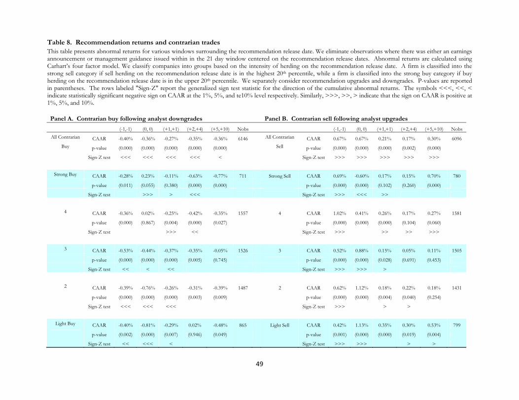
49  

Table 8. Recommendation returns and contrarian tradesThis table presents abnormal returns for various windows surrounding the recommendation release date. We eliminate observations where there was either an earnings announcement or management guidance issued within in the 21 day window centered on the recommendation release dates. Abnormal returns are calculated using Carhart’s four factor model. We classify companies into groups based on the intensity of herding on the recommendation release date. A firm is classified into the strong sell category if sell herding on the recommendation release date is in the highest 20th percentile, while a firm is classified into the strong buy category if buy herding on the recommendation release date is in the upper 20th percentile. We separately consider recommendation upgrades and downgrades. P-values are reported in parentheses. The rows labeled "Sign-Z" report the generalized sign test statistic for the direction of the cumulative abnormal returns. The symbols <<<, <<, < indicate statistically significant negative sign on CAAR at the 1%, 5%, and te10% level respectively. Similarly, >>>, >>, > indicate that the sign on CAAR is positive at 1%, 5%, and 10%.

Panel A. Contrarian buy following analyst downgrades Panel B. Contrarian sell following analyst upgrades (-1,-1) (0, 0) (+1,+1) (+2,+4) (+5,+10) Nobs (-1,-1) (0, 0) (+1,+1) (+2,+4) (+5,+10) Nobs

All Contrarian CAAR -0.40% -0.36% -0.27% -0.35% -0.36% 6146 All Contrarian CAAR 0.67% 0.67% 0.21% 0.17% 0.30% 6096

Buy p-value (0.000) (0.000) (0.000) (0.000) (0.000) Sell p-value (0.000) (0.000) (0.000) (0.002) (0.000)

Sign-Z test <<< <<< <<< <<< < Sign-Z test >>> >>> >>> >>> >>>

Strong Buy CAAR -0.28% 0.23% -0.11% -0.63% -0.77% 711 Strong Sell CAAR 0.69% -0.60% 0.17% 0.15% 0.70% 780

p-value (0.011) (0.055) (0.380) (0.000) (0.000) p-value (0.000) (0.000) (0.102) (0.260) (0.000)

Sign-Z test >>> > <<< Sign-Z test >>> <<< >>

4 CAAR -0.36% 0.02% -0.25% -0.42% -0.35% 1557 4 CAAR 1.02% 0.41% 0.26% 0.17% 0.27% 1581

p-value (0.000) (0.867) (0.004) (0.000) (0.027) p-value (0.000) (0.000) (0.000) (0.104) (0.060)

Sign-Z test >>> << Sign-Z test >>> >> >> >>>

3 CAAR -0.53% -0.44% -0.37% -0.35% -0.05% 1526 3 CAAR 0.52% 0.88% 0.15% 0.05% 0.11% 1505

p-value (0.000) (0.000) (0.000) (0.005) (0.745) p-value (0.000) (0.000) (0.028) (0.691) (0.453)

Sign-Z test << < << Sign-Z test >>> >>> >

2 CAAR -0.39% -0.76% -0.26% -0.31% -0.39% 1487 2 CAAR 0.62% 1.12% 0.18% 0.22% 0.18% 1431

p-value (0.000) (0.000) (0.000) (0.003) (0.009) p-value (0.000) (0.000) (0.004) (0.040) (0.254)

Sign-Z test <<< <<< <<< Sign-Z test >>> > >

Light Buy CAAR -0.40% -0.81% -0.29% 0.02% -0.48% 865 Light Sell CAAR 0.42% 1.13% 0.35% 0.30% 0.53% 799

p-value (0.002) (0.000) (0.007) (0.946) (0.049) p-value (0.001) (0.000) (0.000) (0.019) (0.004)

Sign-Z test << <<< < Sign-Z test >>> >>> > >

50  

Table 9. Regression Analysis of post-recommendation returns This table presents the regression analysis on the cumulative abnormal adjusted returns (CAAR) post-recommendation periods. We eliminate observations where there was either an earnings announcement or management guidance issued within in the 21 day window centered on the recommendation release dates. Abnormal returns are calculated using Carhart’s four factor model. The dependent variables are the CAAR for the (+5,+10) and (+5,+15) windows relative to the day of the recommendation release. Upgrade_buyherd takes the value of one if there was a buy herding on the day of an upgrade recommendation and zero otherwise, while Downgrade_sellherd takes the value of one if there was a sell herding on the day of an downgrade recommendation and zero otherwise. The terms Upgrade_sellherd and Downgrade_buyherd indicate contrarian trades against the recommendations. Upgrade_sellherd takes the value of one if there was a sell herding on the day of an upgrade recommendation and zero otherwise, while Downgrade_buyherd takes the value of one if there was a buy herding on the day of an downgrade recommendation and zero otherwise. Abherdh1 is the abnormal herding measure that is computed using the market model. In each specification, we include 10 lags of the abnormal herding variable. To save space, we do not report the coefficients on these variables. P-values (reported in parentheses) are robust to heterokedasticity and within firm’s correlation.

Model 1 Model 2 Model 3

(+5,+10) (+5,+15) (+5,+10) (+5,+15) (+5,+10) (+5,+15)

Herding on recommendations

Upgrade_buyherd*AbHerd , 1.24% 1.43% 1.01% 1.50%

(0.02) (0.03) (0.09) (0.06)

Downgrade_sellherd*AbHerd , 0.82% 1.58% 0.99% 1.40%

(0.07) (0.01) (0.07) (0.06)

Contrarian trades against recommendations

Upgrade_sellherd*AbHerd , -1.09% -2.90% -1.03% -2.82%

(0.02) (0.00) (0.07) (0.00)

Downgrade_buyherd*AbHerd , -1.56% -2.01% -1.57% -2.01%

(0.00) (0.00) (0.01) (0.01)

Intercept -0.05% 0.00% -0.01% -0.04% 0.01% -0.03%

(0.41) (0.99) (0.93) (0.61) (0.95) (0.81)

Rt 2.11% -0.01% 3.10% -0.01% 2.05% -0.15%

(0.28) (1.00) (0.08) (1.00) (0.29) (0.95)

Rt-1 1.62% 2.16% 1.24% 2.16% 1.28% 1.52%

(0.38) (0.34) (0.50) (0.34) (0.49) (0.50)

Lagged Abnormal Herding Included Included Included Included Included Included

R-square 0.204% 0.151% 0.238% 0.247% 0.303% 0.315%

Nobs 26232 26232 26232 26232 26232 26232

51  

Table 10. Recommendation returns and herding for all 1995-2006 observations This table presents buy-and-hold abnormal portfolio returns formed based on the herding measure for 1995-2006. We sort the stocks into their daily deciles portfolio based on their herding measures. We then perform buy-and-hold abnormal return analysis for the days with strong buy and sell herding. Abnormal returns are calculated using the Carhart’s four factor model. P-values are reported in parentheses and are calculated based on the Newey-West t-statistics with 10 days cross correlations.

(-1,-1) Portfolio

formation day (+1,+1) (+2,+4) (+5,+10) Nobs

All Sizes - Equally weighted portfolio

Strong Sell CAAR -0.032% -1.429% -0.032% 0.057% 0.109% 2889

p-value (0.001) (0.000) (0.001) (0.016) (0.011)

Strong Buy CAAR 0.060% 1.388% 0.065% 0.018% 0.019% 2889

p-value (0.000) (0.000) (0.000) (0.453) (0.660)

Strong Buy - Strong Sell CAAR 0.05% 1.41% 0.05% -0.02% 0.06% 2889

p-value (0.000) (0.000) (0.000) (0.003) (0.120)

All Sizes - Value weighted portfolio

Strong Sell CAAR 0.028% -0.721% -0.012% 0.041% 0.023% 2889

p-value (0.610) (0.000) (0.023) (0.734) (0.023)

Strong Buy CAAR 0.047% 0.595% -0.014% 0.078% -0.116% 2889

p-value (0.000) (0.000) (0.013) (0.000) (0.000)

Strong Buy - Strong Sell CAAR 0.02% 1.32% 0.00% -0.12% -0.09% 2889

p-value (0.026) (0.000) (0.810) (0.000) (0.030)

52  

Figure 1. Abnormal herding around analyst recommendations

This figure plots average abnormal herding around recommendation changes. Day 0 corresponds to the release date of the recommendation. We focus on a window from (-10, +10) surrounding the recommendation release date. Recommendations

‐3.00

‐2.00

‐1.00

0.00

1.00

2.00

3.00

‐10 ‐9 ‐8 ‐7 ‐6 ‐5 ‐4 ‐3 ‐2 ‐1 0 +1 +2 +3 +4 +5 +6 +7 +8 +9 +10

Upgrades

Downgrades

53  

Figure 2. Difference of opinions surrounding analyst recommendation releases.

This figure presents the level of shares turnover around analyst recommendation upgrades (top plot) and downgrades (bottom plot). Following Garfinkel (2009), we use trading volume to proxy for opinion divergence. We normalize the turnover to have an initial value of 1 on day t=-10 to facilitate the comparison. The black and white solid columns represent shares turnovers surrounding recommendation releases dates that are accompanied by strong and light institutional herding, respectively. We classify herding into the strong sell (buy) category if sell (buy) herding on the recommendation release date is in the highest quintile. Light buy and sell herding are defined similarly but using the lowest herding quintile. The solid red columns represent the shares turnovers surrounding recommendation releases dates that are accompanied by strong institutional contrarian trades. Strong contrarian sell (buy) trades are when we observe strong institutional sell (buy) herding in the directions that are opposite to the analyst recommendations.

 

0.8

1

1.2

1.4

1.6

1.8

2

2.2

2.4

-10 -9 -8 -7 -6 -5 -4 -3 -2 -1 0 1 2 3 4 5 6 7 8 9 10

Shares turnover surrounding recomendation downgrades

Strong sell herd

Light sell herd

Strong contrarianbuy

0.8

1

1.2

1.4

1.6

1.8

2

-10 -9 -8 -7 -6 -5 -4 -3 -2 -1 0 1 2 3 4 5 6 7 8 9 10

Shares turnover surrounding reccomendation upgrades

Strong buy herd

Light buy herd

Strong contrariansell

54  

Figure 3. Recommendation abnormal returns and Institutional Herding This figure shows the stock price reaction to recommendation upgrades and downgrades stratified by the level of herding. The lines represent the cumulative adjusted abnormal returns (CAAR) that are computed using the Cahart’s (1997) four factor model.Strong buy herding is defined as buy herding in the top quintile, while strong sell herding is defined as herding in the bottom quintile.

-6.00%

-4.00%

-2.00%

0.00%

2.00%

4.00%

6.00%

8.00%

‐10 ‐9 ‐8 ‐7 ‐6 ‐5 ‐4 ‐3 ‐2 ‐1 0 1 2 3 4 5 6 7 8 9

10

11

12

13

14

15

16

17

18

19

20

Strong Buy - Upgrade Strong Sell - Upgrade

Strong Sell - Downgrade Strong Buy - Downgrade