Informative Priors on Fetal Fraction Increase Power of

The Noninvasive Prenatal Screen

Hanli Xu1,8 PhD, Shaowei Wang2,8,9 MD, Lin-Lin Ma2 MD, Shuai Huang2 MD, Lin Liang2 MD,Qian Liu3 PhD, Yang-Yang Liu3 BS, Ke-Di Liu3,4 PhD, Ze-Min Tan3 PhD,

Hao Ban5,6 MD, Yongtao Guan5,6,7,9 PhD, and Zuhong Lu1,9 PhD

1 Department of Biomedical Engineering, Southeast University

2 Department of Obstetrics and Gynecology, Beijing Hospital

3 Beijing USCI Medical Laboratory

4 Department of Biochemistry & Cambridge Systems Biology Centre, University of Cambrdige

5 USDA/ARS Children’s Nutrition Research Center

6 Department of Pediatrics, Baylor College of Medicine

7 Department of Molecular and Human Genetics, Baylor College of Medicine

8 These authors contribute equally.

9 Correspondence: SW: w sw999@163.com, YG: yongtaog@bcm.edu, ZL: zhlu@seu.edu.cn

Mailing address of YG: 1100 Bates Room 2070, Houston TX 77030Tel: 713-798-0362, Fax: 713-798-7098

Running title: Informative priors increase power of the NIPS

1

Abstract

Purpose: The noninvasive prenatal screen (NIPS) sequences a mixture of the maternal and fetal

cell-free DNA. Fetal trisomy can be detected by examining chromosomal dosages estimated from

sequencing reads. Traditional method uses the Z-test that compares a subject against a set of

euploid controls, where the information of fetal fraction is not fully utilized. Here we present a

Bayesian method that leverages informative priors on fetal fraction.

Method: Our Bayesian method combines the Z-test likelihood and informative priors of fetal

fraction, which are learned from the sex chromosomes, to compute Bayes factors. Bayesian frame-

work can account for non-genetic risk factors through the prior odds, and our method can report

individual positive/negative predictive values.

Results: Our Bayesian method has more power than the Z-test method. We analyzed 3405 NIPS

samples and spotted at least 9 (out of 51) possible Z-test false positives.

Conclusion: Bayesian NIPS is more powerful than the Z-test method, is able to account for

non-genetic risk factors through prior odds, and can report individual positive/negative predictive

values.

Keywords: noninvasive, prenatal, prior, fetal fraction, Bayes factor

2

INTRODUCTION

In 1997, Dennis Lo and colleagues discovered the existence of fetus’s cell-free DNA in the plasma

of the maternal peripheral blood [1]. They used PCR to amplify a segment that is unique to the

human Y-chromosome, so that the PCR signal detected has to come from a male fetus. This land-

mark discovery laid the foundation for the noninvasive prenatal screen (NIPS). In 2008, more than

a decade later during which massively parallel sequencing technologies have made rapid progress,

Stephen Quake group and Dennis Lo group, a couple months apart, reported independent successes

in detecting trisomy fetus by sequencing cell-free DNA in maternal peripheral plasma [2, 3]. Follow-

ing these reports, multiple clinical trials demonstrated more than convincingly the benefit of NIPS

over the traditional screen in detecting fetal trisomy [4–6]. And the next-generation sequencing

based NIPS has been rapidly integrated into prenatal care.

In light of compelling new evidence, professional societies endorsed NIPS over the traditional

trisomy screen [7–11]. Particularly, American College of Medical Genetics and Genomics (ACMG)

recently revised their early position of restricting NIPS to high-risk patients [12] to recommend

“NIPS can replace conventional screening for Patau, Edwards, and Down syndromes across the

maternal age spectrum, for a continuum of gestational age beginning at 9–10 weeks, and for patients

who are not significantly obese [11].” The recommendation for gestational age and maternal weight

is to ensure that the fetal fraction (the proportion of cell-free DNA that is originated from the fetus)

is large enough for NIPS to be e↵ective. ACMG emphasizes the importance of the fetal fraction

and recommends: “All laboratories should include a clearly visible fetal fraction on NIPS reports.”

Multiple studies pointed out that the fetal fraction plays a crucial role in e↵ectiveness of NIPS to

detect trisomy [13–16]. The consensus for the detecting limit of fetal fraction appears to be 4%,

although theoretical studies suggested 2% also works [14], and more optimistic authors suggested

that as long as GC bias is accounted for and sequence depth is unlimited, NIPS can be e↵ective

for an arbitrarily small fraction of fetal DNA [17].

The prevailing method used to analyze NIPS datasets, first outlined in [3], is the Z-test method,

which calculates a Z-score that measures deviation of a chromosomal dosage from a set of euploid

control samples. The Z-test pays no special attention to the fetal fraction, other than that the

deviation approximately equals the fetal fraction for a trisomy fetus. (For an euploid fetus, the

deviation is approximately 0.) A chromosomal dosage can be estimated reliably from low-coverage

sequencing reads (Supplementary Material and Methods). NIPS uses euploid control samples to

define baseline. Their chromosomal dosages are estimated, the sample mean µ and the sample

standard deviation (SSD) � are computed, where µ is expected to be 2, but varies slightly from

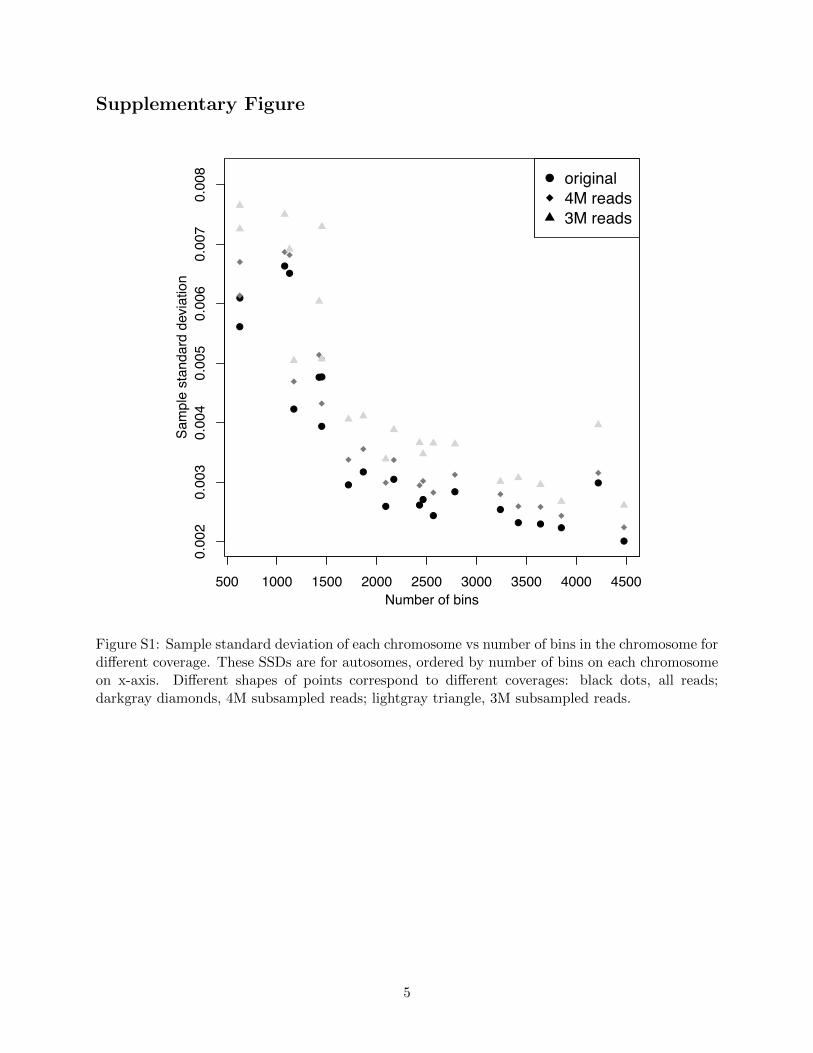
chromosome to chromosome, and di↵erent chromosomes have markedly di↵erent � estimates (Fig-

ure S1). Suppose an euploid mother carries a fetus, and denote c the estimated dosage of an

autosome. Let h be the fetal fraction, then c is expected to be µ + h when the fetus is trisomy,

3

and µ� h when the fetus is monosomy. We have either h = c� µ (for trisomy) or �h = c� µ (for

monosomy); combined together, h = |c� µ|. Define x = c� µ, which is the centered chromosomal

dosage, then |x| is an unbiased estimator of h for a trisomy or monosomy fetus. (Note when the

fetus is euploid, x is expected to be 0 and irrelevant to h.) The Z-score is defined as Z = x/�.

Obviously, a larger h tends to produce a more significant Z-score.

We identify three inadequacies of the Z-test method in NIPS. First, the Z-score is measured

relative to �. An euploid control sample may have an x estimate that is small enough to appear by

chance, but large enough relative to � such that a significant Z-score is obtained, resulting a false

positive. Second, it is well-known that fetal trisomy has an increase risk with respect to maternal

age [18]. The Z-test method has di�culty to incorporate such information. Third, with Z-score

one has to specify a threshold to call positives, negatives, and no calls. But such a threshold

varies for di↵erent investigators [3, 19] and varies even for the same investigators over time [3, 4].

Here we develop a Bayesian method and demonstrate its advantage over the Z-test method through

analyzing a real dataset. The Bayesian method allows us to emphasize the fetal fraction — through

informative priors. The informative priors e↵ectively down weights a Z-score whose corresponding

|x| is small. This alleviates the first inadequacy of the Z-test method. The test statistic produced

by the Bayesian method is Bayes factor [20]. Bayes factor is the change of odds (of trisomy) in light

of the data, and we can compute posterior odds of trisomy by multiplying Bayes factor with prior

odds of trisomy. The prior odds can be the age-adjusted prevalence of trisomy of an autosome. This

addresses the second inadequacy of the Z-test method. From the posterior odds, we can compute

and report the positive predictive value (PPV) and the negative predictive value (NPV). Because

both PPV and NPV are probabilities, they are easily interpretable and more informative than a

Z-score. This mitigates the third inadequacy of the Z-test method.

4

MATERIAL AND METHODS

In Supplementary Material and Methods we documented how patients were recruited and data

collected, details on reads quality control, how we decided the optimal bin sizes when binning

reads together, the hidden Markov model we used to remove maternal CNV and as well as regions

harboring CNV at the population level due to reference bias, details on how we accounted for

GC bias, how we inferred fetal fractions from sex chromosomes, how we fit candidate probability

densities to empirical distribution of fetal fractions and the densities we obtained, how to compute

Bayes factor, and how we simulated chromosomal dosages to compare Bayes factors against Z-

scores.

Code availability

R codes implementing methods described in the paper are available upon request.

5

RESULTS

Fetal fractions

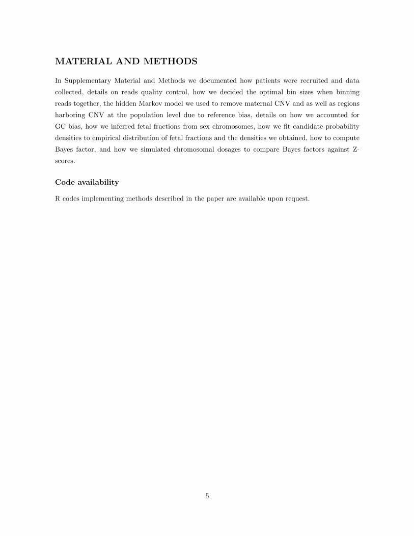
We first inferred fetal fractions (denoted by h) for each sample using sex chromosomes. The

empirical distributions of these fetal fractions were used to formulate our informative priors for

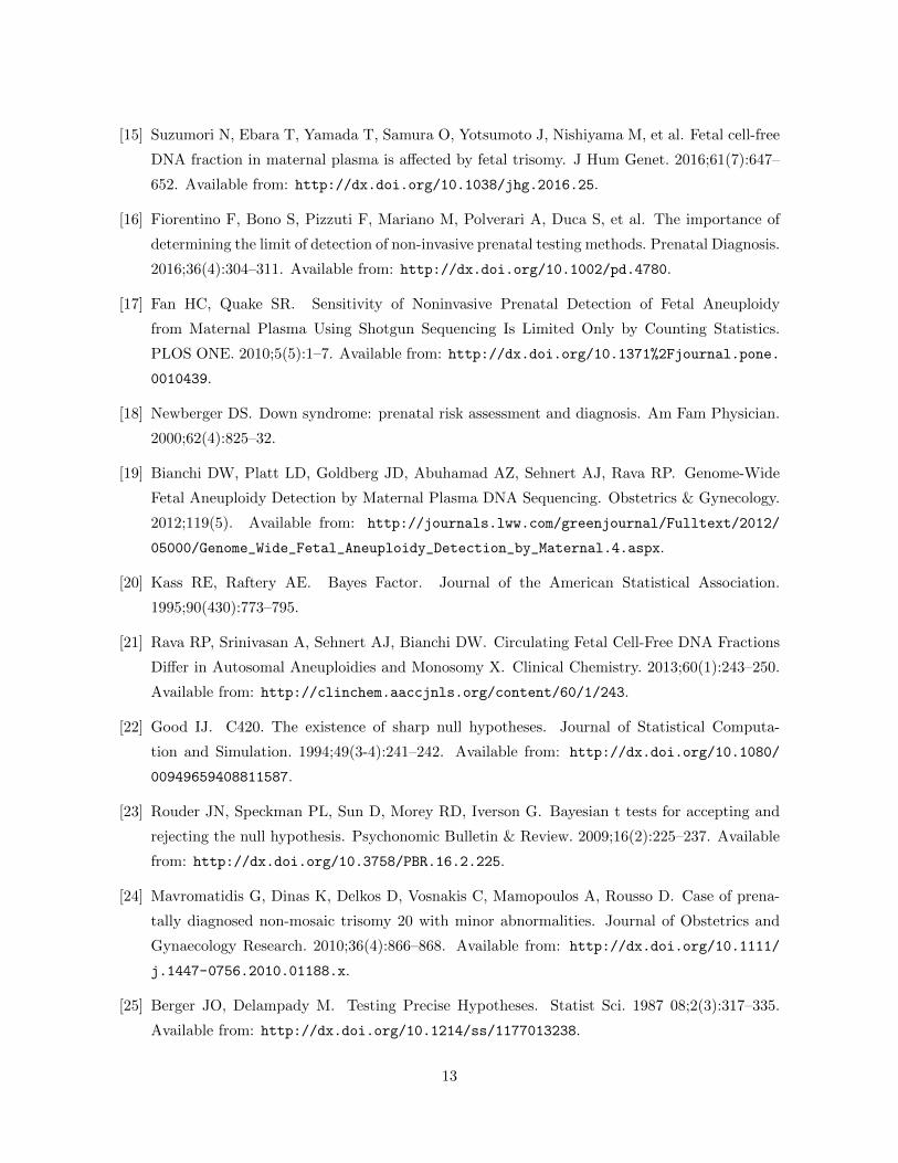
Bayesian analysis. For a female fetus the expected chromosome X and Y dosages are 2 and 0

respectively, and fetal fraction of a female fetus estimated from sex chromosomes is expected to

be 0. For a male fetus, the expected X dosage is 2 � h and the expected Y dosage is h. Thus,

both X and Y dosages are informative to the fetal fraction of a male fetus. Our data suggested

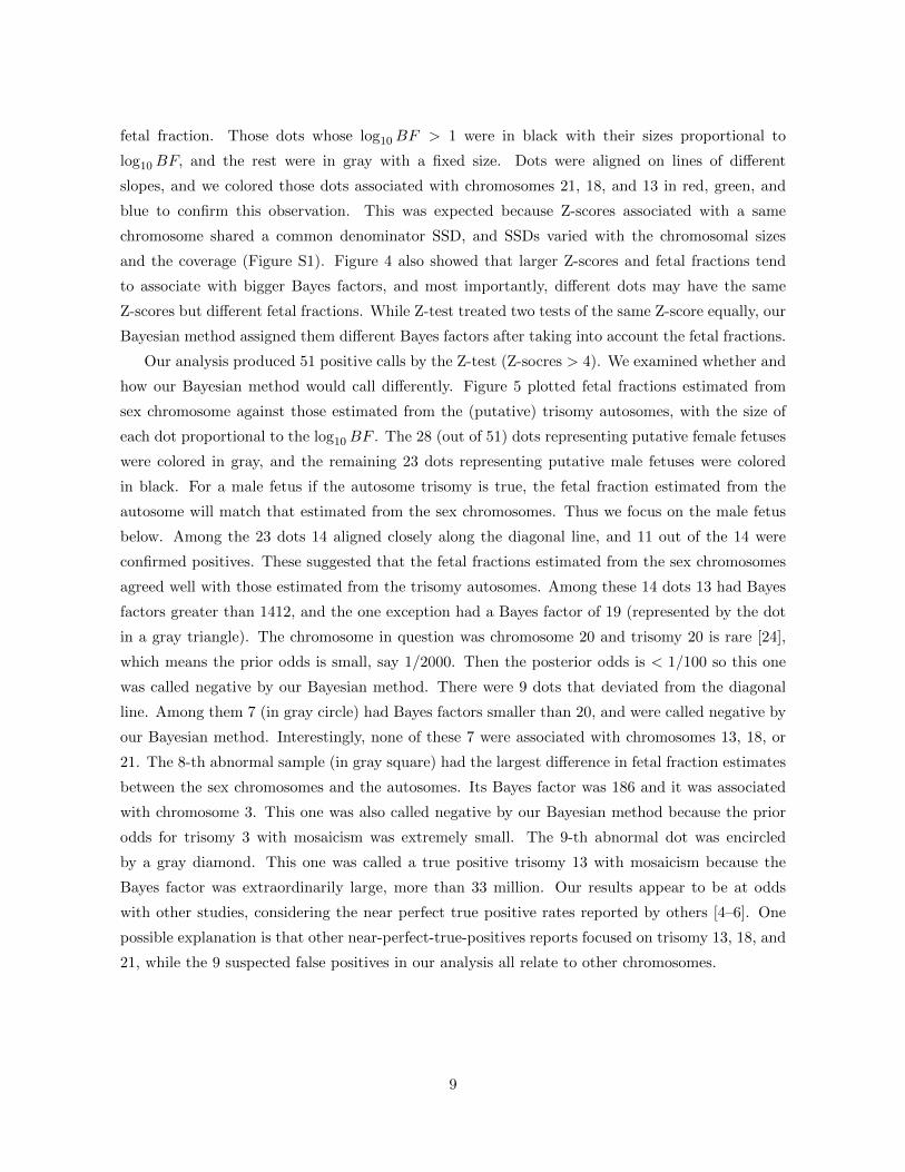
that the Y dosage is more informative than the X dosage (Figure 1a). We estimated the fetal

fractions for all samples using both X and Y dosages (Supplementary Materials and Methods).

Figure 1b showed the histograms of the inferred fetal fraction (on the log scale). The two modes

correspond to putative female and male fetuses. To avoid arbitrariness in specifying a threshold, we

used the K-means method to divide the log fetal fractions into two groups. The inferred threshold

of fetal fraction is 0.028. Among 3405 samples analyzed, 1693 (49.7%) had fetal fractions greater

than 0.028 and thus carrying putative male fetuses, and the remaining 1712 (50.3%) samples were

carrrying putative female fetuses.

Taking fetal fraction estimates from samples carrying putative male fetuses, we digressed to

investigate how maternal age, gestational age, and maternal weight a↵ect the log fetal fraction.

Because these investigations relied on the linear regression, we used log fetal fraction instead of fetal

fraction, as the former was a better fit to a normal distribution, which is the basic assumption for

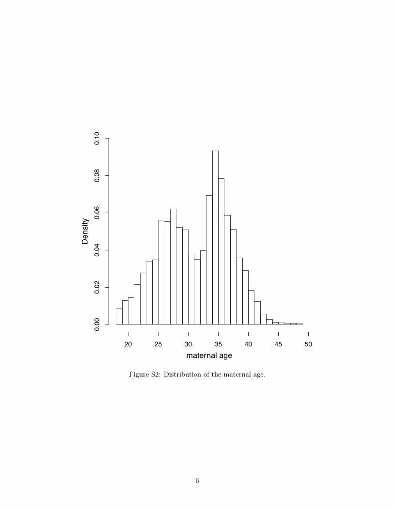
linear regression. Maternal age in our sample followed a bimodal distribution, with two modes at 27

and 35 years of age (Figure S2). Evidently, women in their late child-bearing ages took advantage

of the new “two child policy” in China e↵ective since 1 January 2016. Simple linear regression

suggested an association between maternal age and log fetal fraction (P = 6.0 ⇥ 10�10), but the

association disappeared after controlling for gestational age and maternal weight (P = 0.12). This

non-association agrees with a previous study using American samples of European descents [21].

The gestational age is positively associated with the log fetal fraction (P = 7.2 ⇥ 10�24) and

maternal weight is negatively associated with the log fetal fraction (P = 4.0⇥ 10�49). Both agree

with earlier studies [2, 13]. Gestational age accounts for 4.2% variation of log fetal fraction and

maternal weight accounts for 13.9%, and combined they account for 15.4%.

Prior specification

The computation of Bayes factor requires one to integrate the likelihood, which contains data and

the parameter (fetal fraction here), over the prior distributions of the parameter, separately for

the null and alternative models (Supplementary Materials and Methods). Thus, we need to specify

6

and justify priors for both null (euploidy) and alternative (trisomy) models. Indeed, the art of

Bayesian methods is prior specification. (The toil of Bayesian methods is computation, but for our

application the computation is rather simple.) The expected fetal fraction estimated from the sex

chromosomes for a putative female fetus is 0, and the observed variation of the estimates can be

regarded as the variation under the null model. The fetal fractions of male fetuses can be reliably

estimated from the sex chromosomes (in the absence of mosaicism), and the observed variation can

be regarded as the variation under the alternative model. After visual inspection of the histograms,

we elected to use Beta and Log-Normal (LogN) distributions to fit the empirical distributions of

the fetal fractions. With fetal fractions of putative female fetuses, the fitted density was denoted by

g

⇤0; with those of putative male fetuses, g⇤1; and with those of female and male fetuses combined, g⇤2,

where ⇤ can be either B (for Beta) or L (for LogN). The parameters of the fitted distributions were

determined by matching the means and the variances of an empirical distribution and a candidate

distribution. The explicit forms of the fitted distributions can be found in the Supplementary

Materials and Methods, and Figure 1b demonstrated the goodness of fit.

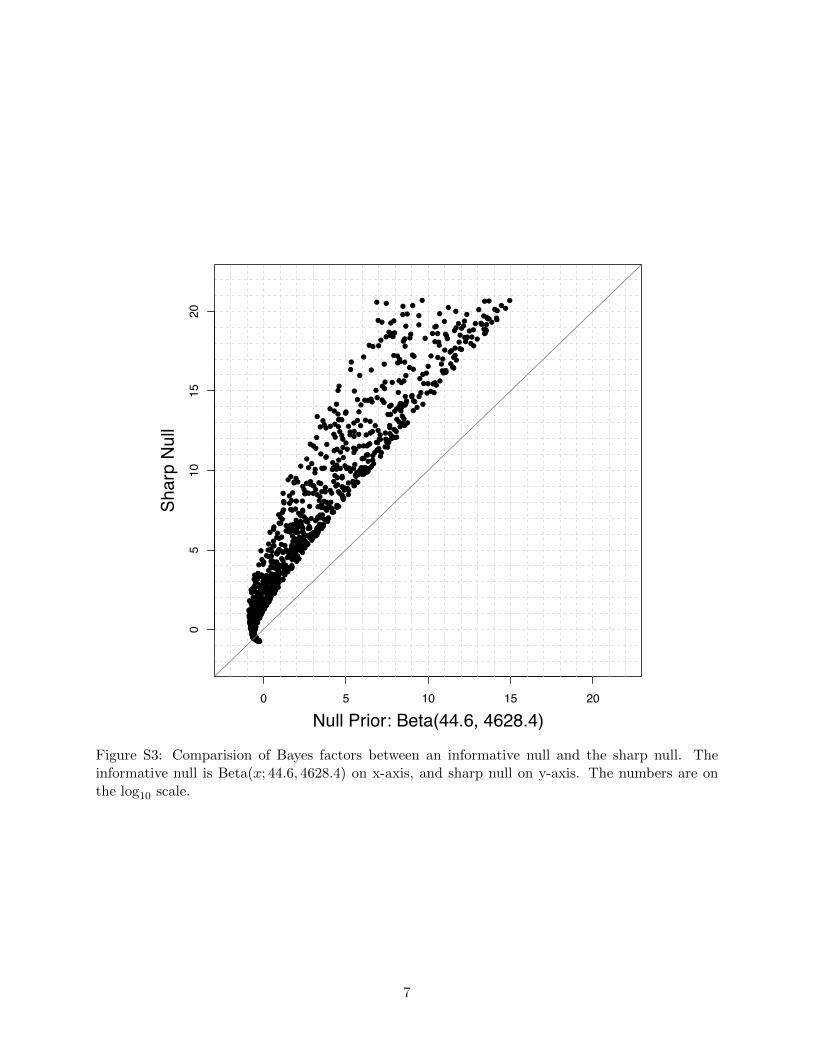
Using the sharp null is common practice in Bayesian methods. In our context, the sharp

null specifies the null distribution as a point mass h = 0, as oppose to assuming h following a

distribution that has its density concentrating near 0 but with variations. The sharp null, however,

is a choice often made for convenience rather than merits [22]. In our application, the sharp

null produced much-inflated Bayes factors (Figure S3), which would favor the alternative model

to produce false positives. We thus avoided the sharp null, and instead used g

⇤0 as informative

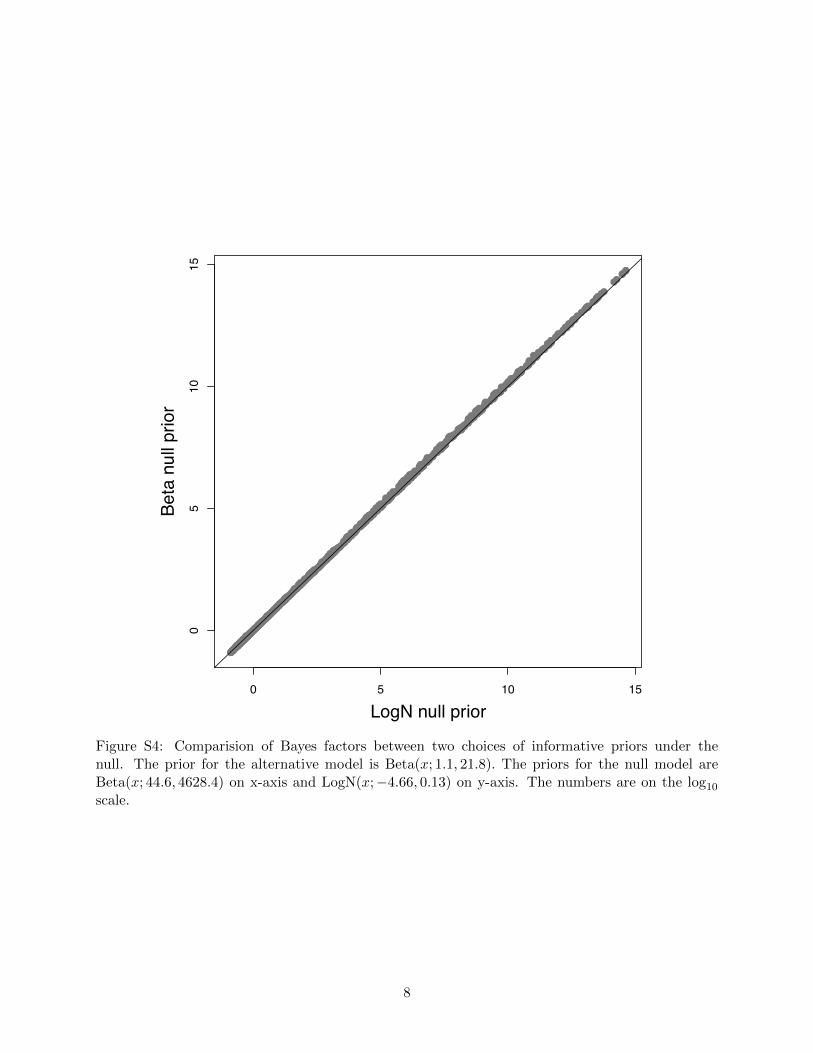
prior for the null model. To choose between Beta (gB0 ) and LogN (gL0 ), we simulated chromosomal

dosages (Supplementary Materials and Methods) and computed Bayes factors (with a prior for

the alternative model to be specified below). Figure S4 showed that the two sets of Bayes factors

were almost identical to each other. We chose g

B0 as the null prior in our data analysis because its

computation is easier.

To specify priors under the alternative model, it was tempting to use g⇤1 as an informative prior.

Standard theory states that the marginal likelihood of a composite hypothesis is the weighted aver-

age of the likelihood over all constituent point hypotheses, where the prior serves as the weight [23].

This gave rise our first concern of using g

⇤1 as prior for the alternative model: g

⇤1 has almost no

weights at or near 0, which risks to be overly against the null model. The second but related

concern was that gB1 placed 10 times more weight at fatal fraction 0.04 than at 0.02, and for gL1 the

weight ratio between the two fetal fractions is 150. Another choice of the prior for the alternative

model was g

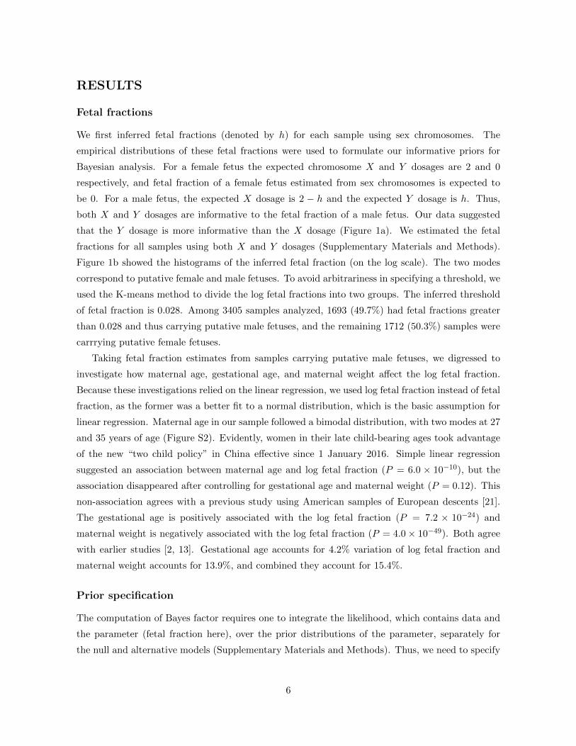
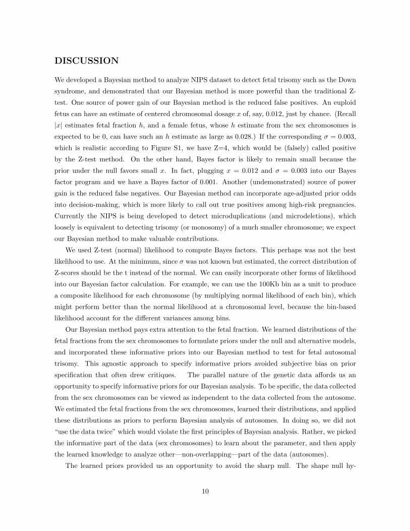
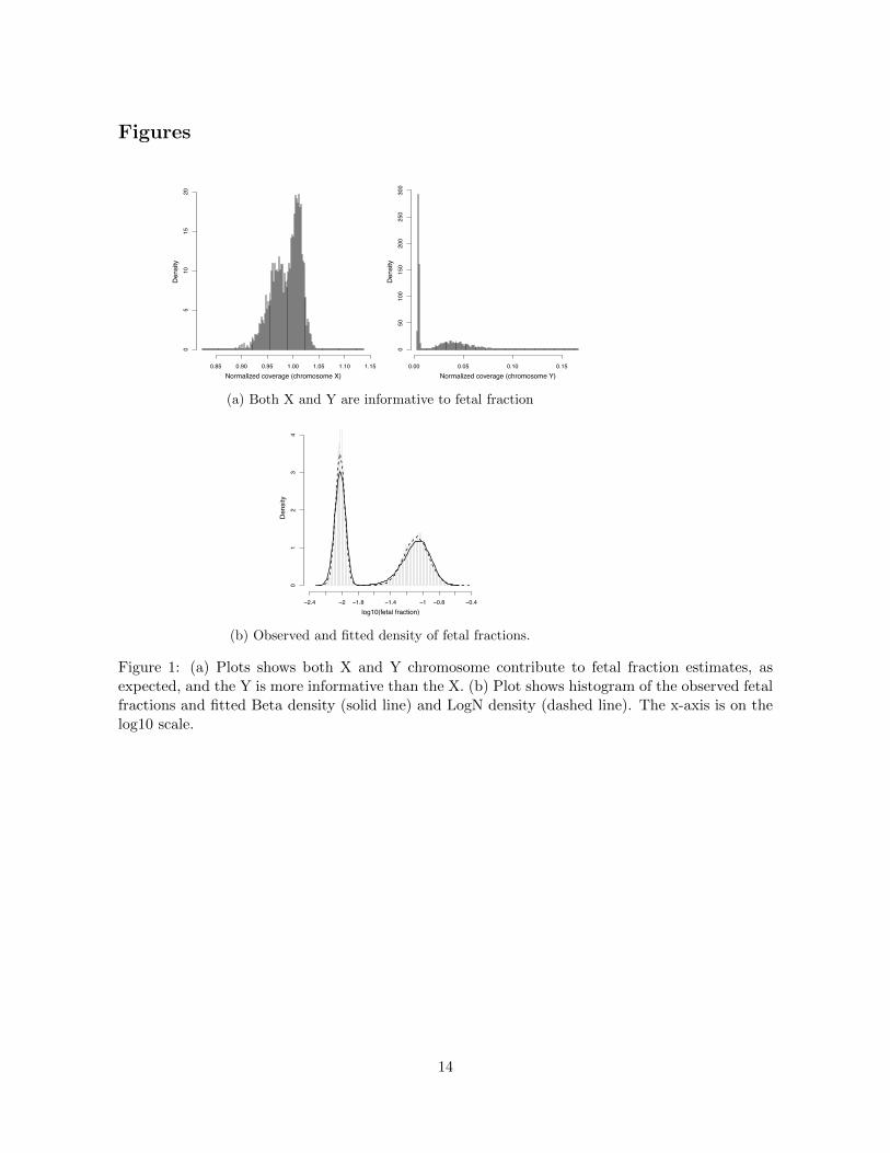
⇤2. We examined the posterior mean of each candidate prior (in light of the Z-test

likelihood) and used which to guide our choice of prior for the alternative model. Figure 2 plotted

the observed fetal fractions and their posterior mean estimates under g

⇤1 and g

⇤2. Priors g

⇤1 over-

estimated the posterior mean for small observed fetal fractions, particularly in region (0.01, 0.05).

Priors g⇤2 performed desirably, with Beta slightly better than LogN. We therefore chose gB2 as prior

7

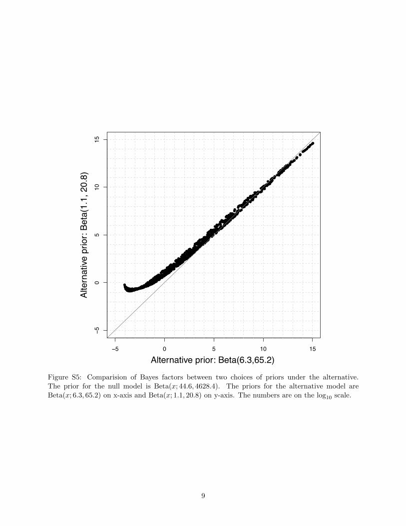
for the alternative model in our data analysis. This prior places 0.7 times weight at fetal fraction

0.04 than at 0.02. (Figure S5 compared g

B1 and g

B2 quantitatively using simulated chromosomal

dosages.)

Bayesian analysis

Data processing produced a pair (x,�) for each autosome of each sample, where x is a centered

chromosomal dosage, and � is the SSD of chromosomal dosages of euploid controls. A Z-score can

be computed via z = x/�. Treating |x| as a one sample estimate of fetal fraction h, we obtained

a normal likelihood, which is the natural likelihood associated with the Z-test. Combining the

likelihood with the priors for h under the null and alternative models we can compute Bayes

factors (Supplementary Materials and Methods). Bayes factor (BF) is the change of odds in light

of data:

Posterior odds of trisomy (!) = Prior odds of trisomy⇥ BF. (1)

It is well-known that the prior odds of fetal trisomy increases with the maternal age [18]. For

example, at age 25 the odds (or the risk/prevalence) of a woman having a child with Down syndrome

is 1/1300; at age 35, the odds increases to 1/365; and at age 45, 1/30. With Bayesian inference this

age-dependent risk can be conveniently incorporated into our analysis. From the posterior odds,

the posterior probability of trisomy (⌧) can be computed by ⌧ = !/(1 + !). Because we choose

between the null and the alternative models, the posterior probability of euploidy is 1 � ⌧. For

a given sample, if it is called positive, then the individual positive predictive value (PPV) is ⌧ .

This is because PPV is a ratio between number of true positives—which is ⌧ in our one sample

situation—and number of all positive calls—which is 1. Similarly, if it is called negative then the

individual negative predictive value (NPV) is 1� ⌧ .

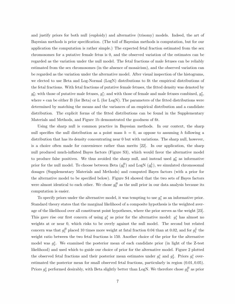
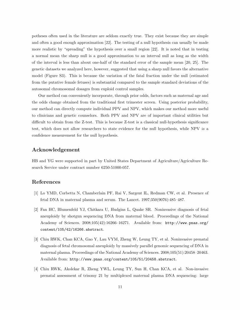
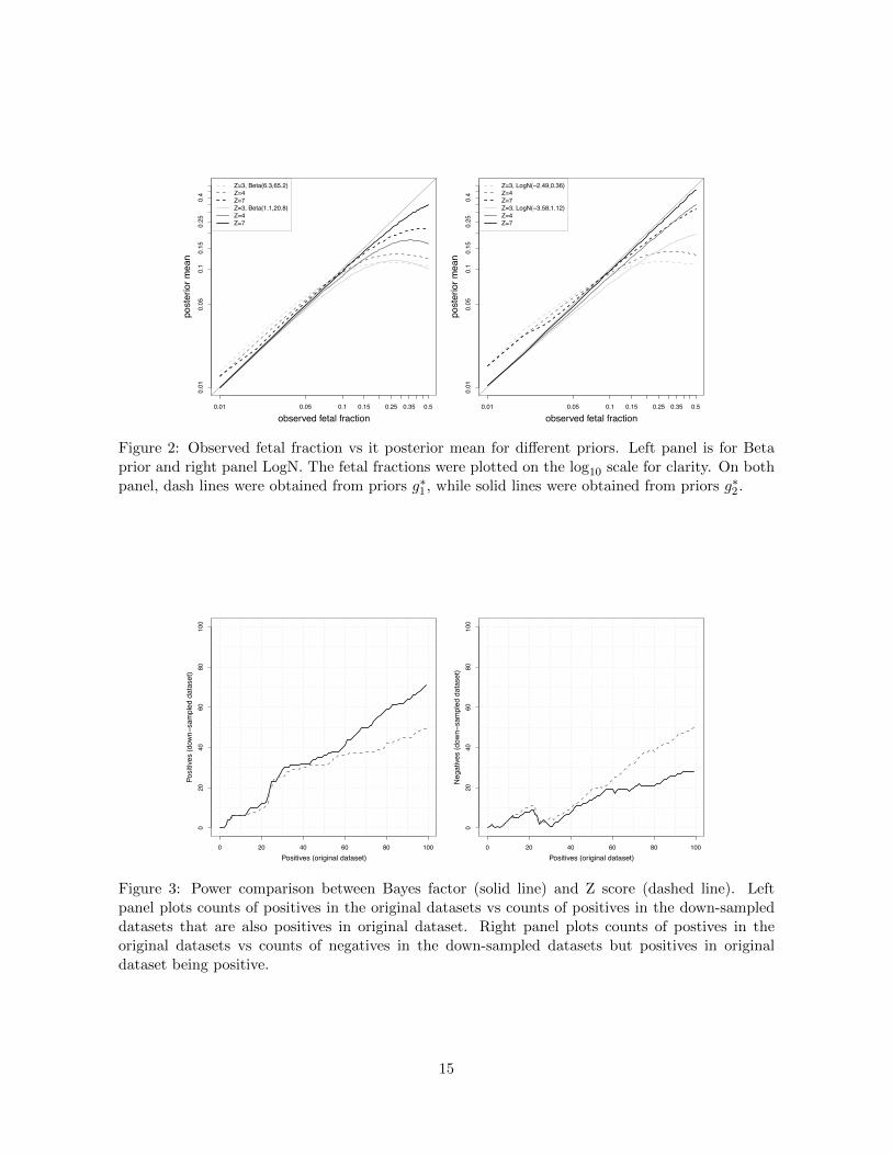
We compared our Bayesian method with the Z-test method by down-sampling reads and ex-

amining the consistency between the original data and the down-sampled data. The counts of

positives/negatives were obtained by varying threshold of test statistics. For log10BF the thresh-

old ranges from 0.67 to 89.60 and for Z score, 3.41 to 21.89. We counted the number of positives

(n+) and number of negatives (n�) in the down-sampled dataset that were positive in the original

dataset. Assuming the positives called in original datasets were the truth, a more powerful method

was expected to have a larger n+ (which mimic true positives) and a smaller n� (which mimic false

negatives). Figure 3 demonstrates that, compared to the Z-test, our Bayesian method produced

more “true positives” and less “false negatives”. In other words, the results were more consistent

between the original data and the down-sampled data when our Bayesian method was used, and

less consistent when the Z-test method was used.

For each autosome of each individual, we calculated a centered chromosomal dosage, estimated

the fetal fraction, and computed a Z-score and a Bayes factor. Figure 4 plotted Z-score against

8

fetal fraction. Those dots whose log10BF > 1 were in black with their sizes proportional to

log10BF, and the rest were in gray with a fixed size. Dots were aligned on lines of di↵erent

slopes, and we colored those dots associated with chromosomes 21, 18, and 13 in red, green, and

blue to confirm this observation. This was expected because Z-scores associated with a same

chromosome shared a common denominator SSD, and SSDs varied with the chromosomal sizes

and the coverage (Figure S1). Figure 4 also showed that larger Z-scores and fetal fractions tend

to associate with bigger Bayes factors, and most importantly, di↵erent dots may have the same

Z-scores but di↵erent fetal fractions. While Z-test treated two tests of the same Z-score equally, our

Bayesian method assigned them di↵erent Bayes factors after taking into account the fetal fractions.

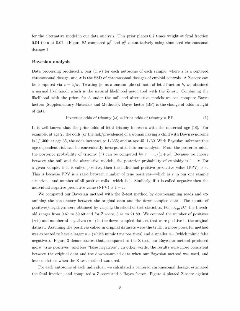
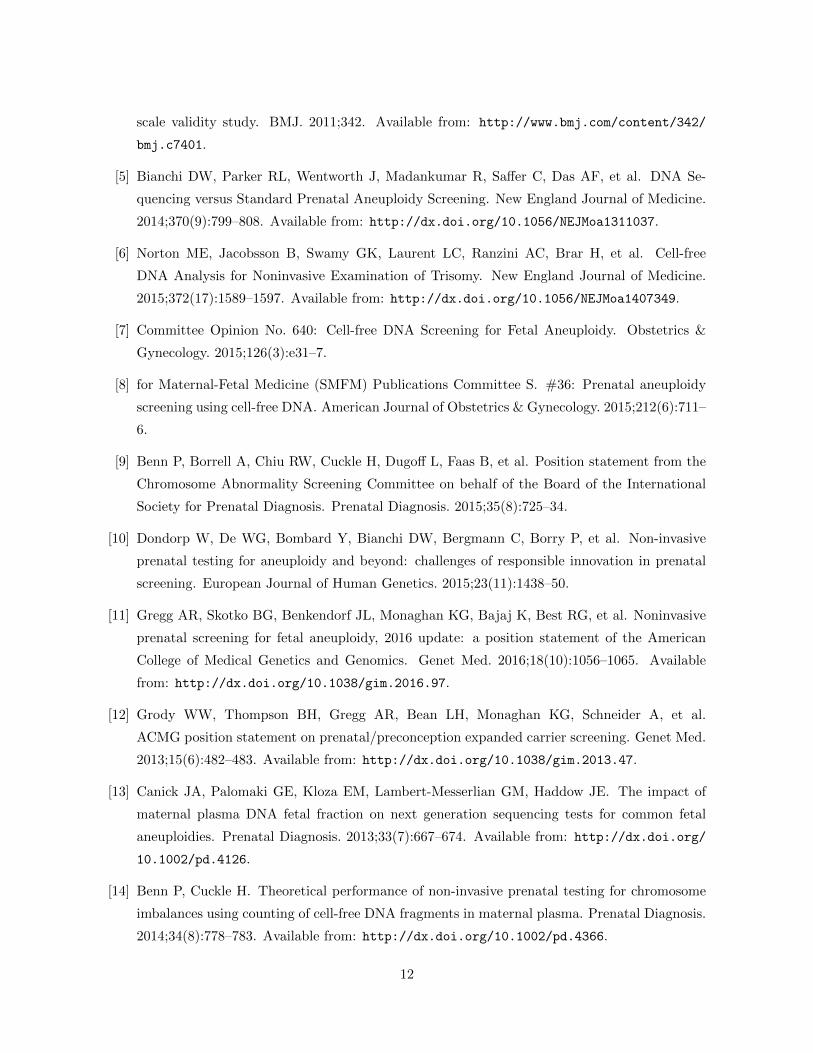
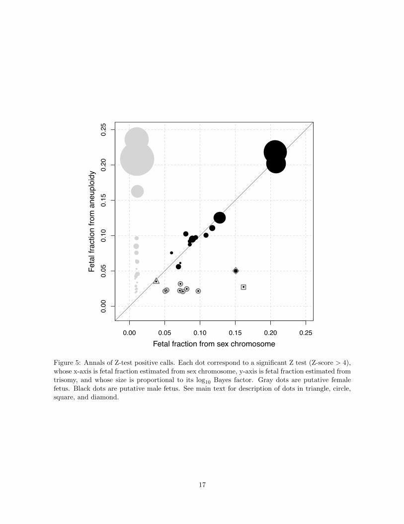
Our analysis produced 51 positive calls by the Z-test (Z-socres > 4). We examined whether and

how our Bayesian method would call di↵erently. Figure 5 plotted fetal fractions estimated from

sex chromosome against those estimated from the (putative) trisomy autosomes, with the size of

each dot proportional to the log10BF . The 28 (out of 51) dots representing putative female fetuses

were colored in gray, and the remaining 23 dots representing putative male fetuses were colored

in black. For a male fetus if the autosome trisomy is true, the fetal fraction estimated from the

autosome will match that estimated from the sex chromosomes. Thus we focus on the male fetus

below. Among the 23 dots 14 aligned closely along the diagonal line, and 11 out of the 14 were

confirmed positives. These suggested that the fetal fractions estimated from the sex chromosomes

agreed well with those estimated from the trisomy autosomes. Among these 14 dots 13 had Bayes

factors greater than 1412, and the one exception had a Bayes factor of 19 (represented by the dot

in a gray triangle). The chromosome in question was chromosome 20 and trisomy 20 is rare [24],

which means the prior odds is small, say 1/2000. Then the posterior odds is < 1/100 so this one

was called negative by our Bayesian method. There were 9 dots that deviated from the diagonal

line. Among them 7 (in gray circle) had Bayes factors smaller than 20, and were called negative by

our Bayesian method. Interestingly, none of these 7 were associated with chromosomes 13, 18, or

21. The 8-th abnormal sample (in gray square) had the largest di↵erence in fetal fraction estimates

between the sex chromosomes and the autosomes. Its Bayes factor was 186 and it was associated

with chromosome 3. This one was also called negative by our Bayesian method because the prior

odds for trisomy 3 with mosaicism was extremely small. The 9-th abnormal dot was encircled

by a gray diamond. This one was called a true positive trisomy 13 with mosaicism because the

Bayes factor was extraordinarily large, more than 33 million. Our results appear to be at odds

with other studies, considering the near perfect true positive rates reported by others [4–6]. One

possible explanation is that other near-perfect-true-positives reports focused on trisomy 13, 18, and

21, while the 9 suspected false positives in our analysis all relate to other chromosomes.

9

DISCUSSION

We developed a Bayesian method to analyze NIPS dataset to detect fetal trisomy such as the Down

syndrome, and demonstrated that our Bayesian method is more powerful than the traditional Z-

test. One source of power gain of our Bayesian method is the reduced false positives. An euploid

fetus can have an estimate of centered chromosomal dosage x of, say, 0.012, just by chance. (Recall

|x| estimates fetal fraction h, and a female fetus, whose h estimate from the sex chromosomes is

expected to be 0, can have such an h estimate as large as 0.028.) If the corresponding � = 0.003,

which is realistic according to Figure S1, we have Z=4, which would be (falsely) called positive

by the Z-test method. On the other hand, Bayes factor is likely to remain small because the

prior under the null favors small x. In fact, plugging x = 0.012 and � = 0.003 into our Bayes

factor program and we have a Bayes factor of 0.001. Another (undemonstrated) source of power

gain is the reduced false negatives. Our Bayesian method can incorporate age-adjusted prior odds

into decision-making, which is more likely to call out true positives among high-risk pregnancies.

Currently the NIPS is being developed to detect microduplications (and microdeletions), which

loosely is equivalent to detecting trisomy (or monosomy) of a much smaller chromosome; we expect

our Bayesian method to make valuable contributions.

We used Z-test (normal) likelihood to compute Bayes factors. This perhaps was not the best

likelihood to use. At the minimum, since � was not known but estimated, the correct distribution of

Z-scores should be the t instead of the normal. We can easily incorporate other forms of likelihood

into our Bayesian factor calculation. For example, we can use the 100Kb bin as a unit to produce

a composite likelihood for each chromosome (by multiplying normal likelihood of each bin), which

might perform better than the normal likelihood at a chromosomal level, because the bin-based

likelihood account for the di↵erent variances among bins.

Our Bayesian method pays extra attention to the fetal fraction. We learned distributions of the

fetal fractions from the sex chromosomes to formulate priors under the null and alternative models,

and incorporated these informative priors into our Bayesian method to test for fetal autosomal

trisomy. This agnostic approach to specify informative priors avoided subjective bias on prior

specification that often drew critiques. The parallel nature of the genetic data a↵ords us an

opportunity to specify informative priors for our Bayesian analysis. To be specific, the data collected

from the sex chromosomes can be viewed as independent to the data collected from the autosome.

We estimated the fetal fractions from the sex chromosomes, learned their distributions, and applied

these distributions as priors to perform Bayesian analysis of autosomes. In doing so, we did not

“use the data twice” which would violate the first principles of Bayesian analysis. Rather, we picked

the informative part of the data (sex chromosomes) to learn about the parameter, and then apply

the learned knowledge to analyze other—non-overlapping—part of the data (autosomes).

The learned priors provided us an opportunity to avoid the sharp null. The shape null hy-

10

potheses often used in the literature are seldom exactly true. They exist because they are simple

and often a good enough approximation [22]. The testing of a null hypothesis can usually be made

more realistic by “spreading” the hypothesis over a small region [22]. It is noted that in testing

a normal mean the sharp null is a good approximation to an interval null as long as the width

of the interval is less than about one-half of the standard error of the sample mean [20, 25]. The

genetic datasets we analyzed here, however, suggested that using a sharp null favors the alternative

model (Figure S3). This is because the variation of the fatal fraction under the null (estimated

from the putative female fetuses) is substantial compared to the sample standard deviations of the

autosomal chromosomal dosages from euploid control samples.

Our method can conveniently incorporate, through prior odds, factors such as maternal age and

the odds change obtained from the traditional first trimester screen. Using posterior probability,

our method can directly compute individual PPV and NPV, which makes our method more useful

to clinicians and genetic counselors. Both PPV and NPV are of important clinical utilities but

di�cult to obtain from the Z-test. This is because Z-test is a classical null-hypothesis significance

test, which does not allow researchers to state evidence for the null hypothesis, while NPV is a

confidence measurement for the null hypothesis.

Acknowledgement

HB and YG were supported in part by United States Department of Agriculture/Agriculture Re-

search Service under contract number 6250-51000-057.

References

[1] Lo YMD, Corbetta N, Chamberlain PF, Rai V, Sargent IL, Redman CW, et al. Presence of

fetal DNA in maternal plasma and serum. The Lancet. 1997;350(9076):485–487.

[2] Fan HC, Blumenfeld YJ, Chitkara U, Hudgins L, Quake SR. Noninvasive diagnosis of fetal

aneuploidy by shotgun sequencing DNA from maternal blood. Proceedings of the National

Academy of Sciences. 2008;105(42):16266–16271. Available from: http://www.pnas.org/

content/105/42/16266.abstract.

[3] Chiu RWK, Chan KCA, Gao Y, Lau VYM, Zheng W, Leung TY, et al. Noninvasive prenatal

diagnosis of fetal chromosomal aneuploidy by massively parallel genomic sequencing of DNA in

maternal plasma. Proceedings of the National Academy of Sciences. 2008;105(51):20458–20463.

Available from: http://www.pnas.org/content/105/51/20458.abstract.

[4] Chiu RWK, Akolekar R, Zheng YWL, Leung TY, Sun H, Chan KCA, et al. Non-invasive

prenatal assessment of trisomy 21 by multiplexed maternal plasma DNA sequencing: large

11

scale validity study. BMJ. 2011;342. Available from: http://www.bmj.com/content/342/

bmj.c7401.

[5] Bianchi DW, Parker RL, Wentworth J, Madankumar R, Sa↵er C, Das AF, et al. DNA Se-

quencing versus Standard Prenatal Aneuploidy Screening. New England Journal of Medicine.

2014;370(9):799–808. Available from: http://dx.doi.org/10.1056/NEJMoa1311037.

[6] Norton ME, Jacobsson B, Swamy GK, Laurent LC, Ranzini AC, Brar H, et al. Cell-free

DNA Analysis for Noninvasive Examination of Trisomy. New England Journal of Medicine.

2015;372(17):1589–1597. Available from: http://dx.doi.org/10.1056/NEJMoa1407349.

[7] Committee Opinion No. 640: Cell-free DNA Screening for Fetal Aneuploidy. Obstetrics &

Gynecology. 2015;126(3):e31–7.

[8] for Maternal-Fetal Medicine (SMFM) Publications Committee S. #36: Prenatal aneuploidy

screening using cell-free DNA. American Journal of Obstetrics & Gynecology. 2015;212(6):711–

6.

[9] Benn P, Borrell A, Chiu RW, Cuckle H, Dugo↵ L, Faas B, et al. Position statement from the

Chromosome Abnormality Screening Committee on behalf of the Board of the International

Society for Prenatal Diagnosis. Prenatal Diagnosis. 2015;35(8):725–34.

[10] Dondorp W, De WG, Bombard Y, Bianchi DW, Bergmann C, Borry P, et al. Non-invasive

prenatal testing for aneuploidy and beyond: challenges of responsible innovation in prenatal

screening. European Journal of Human Genetics. 2015;23(11):1438–50.

[11] Gregg AR, Skotko BG, Benkendorf JL, Monaghan KG, Bajaj K, Best RG, et al. Noninvasive

prenatal screening for fetal aneuploidy, 2016 update: a position statement of the American

College of Medical Genetics and Genomics. Genet Med. 2016;18(10):1056–1065. Available

from: http://dx.doi.org/10.1038/gim.2016.97.

[12] Grody WW, Thompson BH, Gregg AR, Bean LH, Monaghan KG, Schneider A, et al.

ACMG position statement on prenatal/preconception expanded carrier screening. Genet Med.

2013;15(6):482–483. Available from: http://dx.doi.org/10.1038/gim.2013.47.

[13] Canick JA, Palomaki GE, Kloza EM, Lambert-Messerlian GM, Haddow JE. The impact of

maternal plasma DNA fetal fraction on next generation sequencing tests for common fetal

aneuploidies. Prenatal Diagnosis. 2013;33(7):667–674. Available from: http://dx.doi.org/

10.1002/pd.4126.

[14] Benn P, Cuckle H. Theoretical performance of non-invasive prenatal testing for chromosome

imbalances using counting of cell-free DNA fragments in maternal plasma. Prenatal Diagnosis.

2014;34(8):778–783. Available from: http://dx.doi.org/10.1002/pd.4366.

12

[15] Suzumori N, Ebara T, Yamada T, Samura O, Yotsumoto J, Nishiyama M, et al. Fetal cell-free

DNA fraction in maternal plasma is a↵ected by fetal trisomy. J Hum Genet. 2016;61(7):647–

652. Available from: http://dx.doi.org/10.1038/jhg.2016.25.

[16] Fiorentino F, Bono S, Pizzuti F, Mariano M, Polverari A, Duca S, et al. The importance of

determining the limit of detection of non-invasive prenatal testing methods. Prenatal Diagnosis.

2016;36(4):304–311. Available from: http://dx.doi.org/10.1002/pd.4780.

[17] Fan HC, Quake SR. Sensitivity of Noninvasive Prenatal Detection of Fetal Aneuploidy

from Maternal Plasma Using Shotgun Sequencing Is Limited Only by Counting Statistics.

PLOS ONE. 2010;5(5):1–7. Available from: http://dx.doi.org/10.1371%2Fjournal.pone.

0010439.

[18] Newberger DS. Down syndrome: prenatal risk assessment and diagnosis. Am Fam Physician.

2000;62(4):825–32.

[19] Bianchi DW, Platt LD, Goldberg JD, Abuhamad AZ, Sehnert AJ, Rava RP. Genome-Wide

Fetal Aneuploidy Detection by Maternal Plasma DNA Sequencing. Obstetrics & Gynecology.

2012;119(5). Available from: http://journals.lww.com/greenjournal/Fulltext/2012/

05000/Genome_Wide_Fetal_Aneuploidy_Detection_by_Maternal.4.aspx.

[20] Kass RE, Raftery AE. Bayes Factor. Journal of the American Statistical Association.

1995;90(430):773–795.

[21] Rava RP, Srinivasan A, Sehnert AJ, Bianchi DW. Circulating Fetal Cell-Free DNA Fractions

Di↵er in Autosomal Aneuploidies and Monosomy X. Clinical Chemistry. 2013;60(1):243–250.

Available from: http://clinchem.aaccjnls.org/content/60/1/243.

[22] Good IJ. C420. The existence of sharp null hypotheses. Journal of Statistical Computa-

tion and Simulation. 1994;49(3-4):241–242. Available from: http://dx.doi.org/10.1080/

00949659408811587.

[23] Rouder JN, Speckman PL, Sun D, Morey RD, Iverson G. Bayesian t tests for accepting and

rejecting the null hypothesis. Psychonomic Bulletin & Review. 2009;16(2):225–237. Available

from: http://dx.doi.org/10.3758/PBR.16.2.225.

[24] Mavromatidis G, Dinas K, Delkos D, Vosnakis C, Mamopoulos A, Rousso D. Case of prena-

tally diagnosed non-mosaic trisomy 20 with minor abnormalities. Journal of Obstetrics and

Gynaecology Research. 2010;36(4):866–868. Available from: http://dx.doi.org/10.1111/

j.1447-0756.2010.01188.x.

[25] Berger JO, Delampady M. Testing Precise Hypotheses. Statist Sci. 1987 08;2(3):317–335.

Available from: http://dx.doi.org/10.1214/ss/1177013238.

13

Figures

0.85 0.90 0.95 1.00 1.05 1.10 1.15

05

1015

20

Normalized coverage (chromosome X)

Den

sity

0.00 0.05 0.10 0.15

050

100

150

200

250

300

Normalized coverage (chromosome Y)

Den

sity

(a) Both X and Y are informative to fetal fraction

01

23

4

−2.4 −2 −1.8 −1.4 −1 −0.8 −0.4log10(fetal fraction)

Den

sity

(b) Observed and fitted density of fetal fractions.

Figure 1: (a) Plots shows both X and Y chromosome contribute to fetal fraction estimates, asexpected, and the Y is more informative than the X. (b) Plot shows histogram of the observed fetalfractions and fitted Beta density (solid line) and LogN density (dashed line). The x-axis is on thelog10 scale.

14

0.01 0.05 0.1 0.15 0.25 0.35 0.5

0.01

0.05

0.1

0.15

0.25

0.4

observed fetal fraction

post

erio

r mea

nZ=3, Beta(6.3,65.2)Z=4Z=7Z=3, Beta(1.1,20.8)Z=4Z=7

0.01 0.05 0.1 0.15 0.25 0.35 0.5

0.01

0.05

0.1

0.15

0.25

0.4

observed fetal fraction

post

erio

r mea

n

Z=3, LogN(−2.49,0.36)Z=4Z=7Z=3, LogN(−3.58,1.12)Z=4Z=7

Figure 2: Observed fetal fraction vs it posterior mean for di↵erent priors. Left panel is for Betaprior and right panel LogN. The fetal fractions were plotted on the log10 scale for clarity. On bothpanel, dash lines were obtained from priors g⇤1, while solid lines were obtained from priors g⇤2.

0 20 40 60 80 100

020

4060

8010

0

Positives (original dataset)

Posi

tives

(dow

n−sa

mpl

ed d

atas

et)

0 20 40 60 80 100

020

4060

8010

0

Positives (original dataset)

Neg

ative

s (d

own−

sam

pled

dat

aset

)

Figure 3: Power comparison between Bayes factor (solid line) and Z score (dashed line). Leftpanel plots counts of positives in the original datasets vs counts of positives in the down-sampleddatasets that are also positives in original dataset. Right panel plots counts of postives in theoriginal datasets vs counts of negatives in the down-sampled datasets but positives in originaldataset being positive.

15

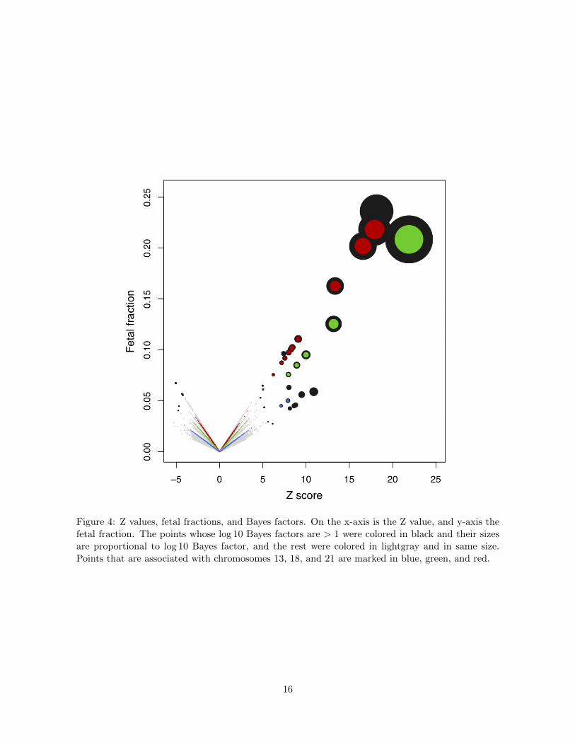
Figure 4: Z values, fetal fractions, and Bayes factors. On the x-axis is the Z value, and y-axis thefetal fraction. The points whose log 10 Bayes factors are > 1 were colored in black and their sizesare proportional to log 10 Bayes factor, and the rest were colored in lightgray and in same size.Points that are associated with chromosomes 13, 18, and 21 are marked in blue, green, and red.

16

0.00 0.05 0.10 0.15 0.20 0.25

0.00

0.05

0.10

0.15

0.20

0.25

●●

●

●●

●●

●

●●

●●

●

●

●

●

●

●

●●●

●●

●●

●●

●

●

●●

●

●●

●

●

●●

●

●

●

●●

●

●

●

●●● ●● ●●

●

Fetal fraction from sex chromosome

Feta

l fra

ctio

n fro

m a

neup

loid

y

Figure 5: Annals of Z-test positive calls. Each dot correspond to a significant Z test (Z-score > 4),whose x-axis is fetal fraction estimated from sex chromosome, y-axis is fetal fraction estimated fromtrisomy, and whose size is proportional to its log10 Bayes factor. Gray dots are putative femalefetus. Black dots are putative male fetus. See main text for description of dots in triangle, circle,square, and diamond.

17

Informative Priors on Fetal Fraction Increase Power of

The Noninvasive Prenatal Screen (Supplementary)

Hanli Xu1,8 PhD, Shaowei Wang2,8,9 MD, Lin-Lin Ma2 MD, Shuai Huang2 MD, Lin Liang2 MD,Qian Liu3 PhD, Yang-Yang Liu3 BS, Ke-Di Liu3,4 PhD, Ze-Min Tan3 PhD,

Hao Ban5,6 MD, Yongtao Guan5,6,7,9 PhD, and Zuhong Lu1,9 PhD

1 Department of Biomedical Engineering, Southeast University2 Department of Obstetrics and Gynecology, Beijing Hospital3 Beijing USCI Medical Laboratory4 Department of Biochemistry & Cambridge Systems Biology Centre, University of Cambrdige5 USDA/ARS Children’s Nutrition Research Center6 Department of Pediatrics, Baylor College of Medicine7 Department of Molecular and Human Genetics, Baylor College of Medicine8 These authors contribute equally.9 Correspondence: SW: w-sw999@163.com, YG: yongtaog@bcm.edu, ZL: zhlu@seu.edu.cn

Mailing address of YG: 1100 Bates Room 2070, Houston TX 77030 Tel: 713-798-0362

Supplementary Materials and Methods

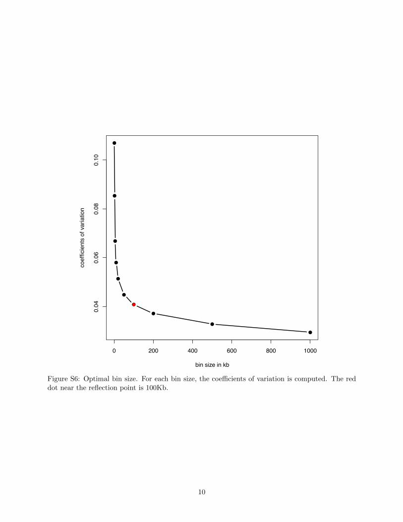
Patients were enrolled, their peripheral blood were drawn, and cell-free DNA were extracted andsequenced (Patients and Data). The study was approved by the institutional review board ofthe Beijing Hospital, Beijing, China. We performed routine quality control for sequencing reads,mapped reads to the reference genome HG19, and retained uniquely mapped reads for furtheranalysis (Reads quality control). After quality control, we had 3405 patients who have more than4M uniquely mapped reads. Because the coverage was low (0.1X), we binned reads for statisticalprocessing before estimating the chromosomal dosages. We examined the coe�cients of variation ofdi↵erent bin sizes (Figure S6), and chose 100Kb as the optimal bin size, which is a balance betweenthe number of bins and the coe�cients of variation (Optimal bin size). We used overlapping binswith two adjacent bins overlapped by 50Kb. The full set of bins is the union of two subsets ofnon-overlapping bins, and we found the overlapping bins improve the stability of the estimates ofchromosomal dosages. Out of concern of reference biases, we developed a hidden Markov model(HMM) to detect and remove bins that suggest putative copy number variation (CNV) at thepopulation level (Remove maternal CNV). We then applied HMM separately for each sample oneach chromosome, and marked those bins that indicate maternal CNV, which were removed fromcomputing chromosomal dosages. (Figure S7 demonstrated an e↵ective detection of a maternalCNV which caused a false positive.) The remaining bins were normalized by their mean coverageto obtain bin dosages. The chromosomal dosage is the average of bin dosages on the chromosome.

We controlled for GC bias and chromosomal bias before estimating chromosomal dosages. Tothis end we only processed autosomes and left out the sex chromosomes. Unlike autosomes, the bindosages on the sex chromosomes depend on fetus’s gender and the fetal fraction even for euploidfetuses. In our data, the bin dosages correlate with bin GC contents in a nonlinear fashion (Fig-ure S8), which makes it ine↵ective to use linear regression to account for GC bias. We applied thesmoothing spline method [1] to e↵ectively remove GC bias (Account for GC bias). For each bin wecomputed mean and variance of GC-corrected bin dosages over all samples, including the possible

1

trisomy samples, and used them as the mean and variance for normal controls. Because of the lowprevalence of trisomy, using all samples as euploid controls produced little bias. For each sample,from GC-corrected bin dosages we regressed out the mean using the weighted linear regression,with the inverse of the variance as the weight. The residuals were used to compute the centeredchromosomal dosages by averaging the residuals over all bins on the chromosome, separately foreach individual. Finally we computed the SSD of each autosome using the centered chromosomaldosages of that chromosome from all samples. For each sample and each autosome, we obtained acentered chromosomal dosage (denoted by x) and the SSD (denoted by �) to test for trisomy.

Patients and Data

Beginning March 15, 2016, we started to enroll pregnant women who were undergoing routineobstetrical care at Beijing Hospital. The institutional review board of the Beijing Hospital approvedthe study. All experiments were performed in accordance with relevant guidelines and regulations.Written informed consent was obtained from all patients. To be eligible for the study, pregnantwomen must be at least 18 years of age and had to be carrying a fetus with a gestational ageof at least 8 weeks. All patients took NIPS test at Beijing Scisoon Medical Laboratory, a partnerclinical test laboratory of Beijing Hospital that is accredited by Beijing Health and Family PlanningCommission. Study inclusion also required accessibility to pregnancy and delivery records, andnewborn physical examination. At enrollment 10 ml peripheral venous blood sample was drawnin a cell-free DNA blood-collection tube. The tube was deidentified and labeled with a uniquebar-code. Samples were shipped the same day to the Beijing Scisoon Medical Laboratory.

Upon receipt, samples were inspected and cell-free plasma was isolated via a double centrifu-gation process of 1600 X g for 10 min, followed by 16000 X g for 10 min. Plasma sample wasfrozen at �80�C until cell-free DNA extraction and sequencing. Cell-free DNA was extracted from600 ul plasma using the Magnetic Serum/Plasma Circulating DNA kit (TIANGEN) according tothe manufacturer’s instructions. Library preparation was processed using NEXTflex Rapid DNASeq Kit (BIOO). After accurate quantification of the number of adatpter-liagted molecules usingKAPA Library Quantification Kits, libraries were pooled and sequenced using Illumine NextSeq500 system according to the manufacturer’s standard protocols. Single end reads of 75-bp wereobtained, and the target coverage is 0.1X.

Reads quality control

Reads were removed the PCR duplicates. A read that contains more than one N were removed.A read is also removed if it contains a consecutive five nucleotides having average Phred score lessthan 20. The remaining reads were mapped to the reference genome (HG19) using BWA, allowingmaximum one mismatch. Only reads that are uniquely mapped were retained for further analysis.A sample passing QC requires minimum of 4M reads that pass QC, although some sample mayhave as many as 10M reads. In our down-sampling experiment, we randomly (uniformly) sample3M reads.

Optimal bin size

The reference genome was divided into 1 Kb non-overlapping bins. Bins contain one or more Nwere removed. We obtained the basepair coverage, and computed the bin coverage by summing thebasepair coverage in the bin. Bins of zero coverage were removed. For each sample, we normalizethe bin coverages using their mean. The normalized bin coverage is called bin dosage. Using allsamples, we computed the mean bin dosage for each bin. We want to determine the optimal bin

2

size using 1 Kb bins as building block. The goal is to balance between the bin size and the numberof bins. We tried bin sizes of 2K, 5K, 10K, 20K, 50K, 100K, 200K, 500K, and 1000K. For eachtarget bin size, we averaged the adjacent 1Kb building-block bins to obtained bin dosages for thenew bins, and computed the coe�cient of variation (the ratio of the standard deviation to themean).

Remove maternal CNV

Let {xm} be a sequence of centered bin dosages for a chromosome. If a bin harbors a maternalCNV, its dosage changes from 0 to 1�h in case of maternal copy number gain of 1 or h� 1 in caseof maternal copy loss of 1, where h is the fetal fraction and usually is < 0.20. We detect such binsusing a hidden Markov model (HMM). The HMM presented here is a simplified version of a previousmodel [2]. The latent variable at each bin consists of three states, copy number loss, neutral, andgain, denoted by -1, 0, and 1 respectively. The latent states along each chromosome form a Markovchain with transition matrix as P (Zm+1 = km+1|Zm = km) = r↵k

m

+ (1� r)1km+1=k

m

, where 1· isthe indicator function, r is the probability such as 1/r is the mean length (in number of bins) of thematernal CNV, and ↵k (for k = �1, 0, 1) are fractions of bins that have copy number loss, neutral,

or gain. And P (Z1 = k) = ↵k. The emission is modeled as P (xm|Zm = k) = 1p2⇡�

k

e� 1

2(x

m

�µ

k

)2

�

2k for

k = �1, 0, 1.We fit the HMM using expectation maximization (EM) algorithm. The forward probabilities

can be computed recursively as

F (m+ 1, Zm+1) = P (x1, . . . , xm, xm+1, Zm+1)

= P (xm+1|Zm+1)X

Zm

F (m,Zm)P (Zm+1|Zm), (1)

with F (1, Z1) = P (x1|Z1). The backward probabilities can be computed recursively as

B(m,Zm) = P (xL, . . . , xm+1|Zm)

=X

Zm+1

P (xm+1|Zm+1)B(m+ 1, Zm+1)P (Zm+1|Zm), (2)

where L is the number of bins, and B(L,ZL) = 1. Then we can compute the posterior probabilitiesof the latent states

zmk = P (Zm = k|x1, . . . , xL) / F (m,Zm = k)B(m,Zm = k). (3)

We can update ↵k =P

m

zmkP

m,k

zmk

. To update µk and �k, we can compute xmzmk for each k to obtain a

L-vector, and then compute the mean of the L-vector as the estimate of µk and compute the SSDthe L-vector as the estimate of �k. We found that using µk = k for k = �1, 0, 1 is convenient andsu�cient because maternal CNV produce the change bin dosages at the magnitude of 1. Finally,we need to specify r. After trial and error, we found r = 0.001 worked well.

Account for GC bias

We first rank all bins on autosome by their GC contents. Then we smooth the bin coverage usingsmooth spline method on the reordered bins, and subtracted the smoothed value o↵ the originalbin dosages. Finally we restore bins to their original order. The processed bin dosages are called

3

GC-corrected bin dosages. Di↵erent chromosomal regions have di↵erent baseline coverages. Whileaccounting for GC bias mitigates the baseline di↵erence, it is far from removing it. We thereforecomputed, for each bin, the mean (m) and variance v of GC-corrected bin dosages over all samples,and regressed out m from GC-corrected bin dosages using weighted linear regression with v asweights.

Infer fetal fraction from sex chromosome dosages

Let h be the fetal fraction, then for a male fetus the expected X chromosome dosage is (2�h) and theexpected Y chromosome dosage is h. Define ⇢ = Y-dosage/X-dosage, then we have ⇢ = h/(2� h),which leads to h = 2⇢/(1 + ⇢). Note when 0 ⇢ < 1, we have 0 h < 1.

Fit probability densities to fetal fractions

The inferred fetal fractions were divided into two groups using the K-means method. Using K-means method is to avoid arbitrariness in specifying a threshold, although visionally identify athreshold will not change the results much. The threshold inferred by the K-means method is0.028. One group whose fetal fractions < 0.028 are putative female fetuses, and the other groupputative male fetuses. The fetal fractions of putative female fetus were fit to a density g0(h), thosefrom male fetus were fit to g1(h), and all fetal fractions were fit to g2(h). After visual inspection,we chose Beta and Log-Normal (LogN) distributions to fit g0, g1, and g2. The parameters weredetermined by matching the first two moments between analytical and empirical distributions. Wearrived at gB0 (h) = Beta(h; 44.6, 4628.4), gB1 (h) = Beta(h; 6.3, 65.2), gL0 (h) = LogN(h;�4.66, 0.13),gL1 (h) = LogN(h;�2.49, 0.36), gB2 (h) = Beta(h; 1.1, 20.8), and gL2 (h) = LogN(h;�3.58, 1.12).

Compute Bayes factors

Under the null H0 : h ⇠ f0(h), and P (D|H0) =RR P (D|h)f0(h)dh. Under the alternative H1 : h ⇠

f1(h), and P (D|H1) =RR P (D|h)f1(h)dh.We compute Bayes factor BF = P (D|H1)

P (D|H0). Recall our data

is a pair D = (x,�), where x is the centered chromosomal dosage, and � is the SSD of chromosomaldosages of controls samples. Treating |x| as one-sample estimate for h we have the likelihood

P (D|h) = 1p2⇡�

exp (� (|x|�h)2

2�2 ). Integrate out prior on h to obtain P (D|Hj) =RR P (D|h)fj(h)dh =

RR

1p2⇡�

exp (� (|x|�h)2

2�2 )fj(h)dh. This Bayes factor calculation can be applied to both trisomy and

monosomy alternative models.

Simulate chromosomal dosages

The goal is to simulated a pair (x, s), where x is the centered chromosomal dosage and s is SSDof euploid control samples, such that Z = x/s has a big spread and s varies in a reasonable range.We simulated z ⇠ Unif(1, 10) and s ⇠ Unif(0.003, 0.008) and obtained x = z ⇥ s. The range of s isclose to what was observed in real data (Figure S1).

References

[1] Hastie T, Tibshirani R. Statistical Science. 1986;1(3):297–318.

[2] Xu H, Guan Y. Detecting Local Haplotype Sharing and Haplotype Association. Genetics.2014;197(3):823–838.

4

Supplementary Figure

●

●

●●●

●●

●

●●

●

●

●

●

●

●

●●

●

●

●

●

0.00

20.

003

0.00

40.

005

0.00

60.

007

0.00

8

500 1000 1500 2000 2500 3000 3500 4000 4500Number of bins

Sam

ple

stan

dard

dev

iatio

n● original

4M reads3M reads

Figure S1: Sample standard deviation of each chromosome vs number of bins in the chromosome fordi↵erent coverage. These SSDs are for autosomes, ordered by number of bins on each chromosomeon x-axis. Di↵erent shapes of points correspond to di↵erent coverages: black dots, all reads;darkgray diamonds, 4M subsampled reads; lightgray triangle, 3M subsampled reads.

5

20 25 30 35 40 45 50

0.00

0.02

0.04

0.06

0.08

0.10

maternal age

Den

sity

Figure S2: Distribution of the maternal age.

6

0 5 10 15 20

05

1015

20

●

●

●

●

●

●

●

●

●

●

●

●

●

●

●

●

●

●

●

●

●

●

●

●

●

●●

●

●

●

●

●

●

●

●

●

●

●

●

●

●

●

●

●

●

●

●

●

●

●

●

●●

●

●

●

●

●

●

●

●

●

●

●

●

●

●

●

●

●

●

●

●

●●

●

●

●

●

●

●

●

●

●

●

●

●

●

●

●

●

●

●

●

●

●

●

●

●●

●

●

●

●

●

●

●

●

●

●

●

●

●

●

●

●

●

●

●

●

●

●

●●●

●

●

●

●

●

●

●

●

●

●

●

●

●●

●

●

● ●

●

●

●

●

●

●

●

●

●

●

●

●

●

●

●

●

●

●

●

●●

●

●

●

●

●

●

●

●

●

●

●

●

●

●

●●

●

●

●

●

●

●

●

●

●

●

●

●

●

●

●

●

●

●

●

●

●

●

●

●

●

●

●

●

●

●

●●

●

●

●

●

●

●

●

●

●

●●

●

●

●

●

●●

●

●

●

●

●

●

●

●

●

●

●

●

●

●

●

●

●

●

●

●

●

●

●

●

●

●

●

●

●

●

●

●

●

●

●

●

●

●

●

●

●

●

●

●

●

●

●

●

●

●

●

●

●

●●

●

●

●

●

●

●

●

●

●

●

●

●●

●

●

●

●

●

●

●

●

●

●

●

●

●

●

●●

●

●

●

●

●

●

●

●

●

●●●

●

●

●

●

●

●

●

●

●

●

●

●

●

●

●

●

●

●

●

●

●

●

●

●

●

●

●

●●●

●

●

●

●

●

●

●

●

●

●

●

●●

● ●

●

●

●

●

●

●

●

●

●

●

●

●

●

●

●

●

●

●

●

●

●

●

●

●

●

●

●

●

●

●

●

●

●●

●

●

●

●

●

●

●

●

●

●

●

●

●

●

●

●

●

●

●●

●

●

●

●

●

●

●

●

●

●

●

●

●

●

●

●

●

●● ●

●

●

●

●

●

●

●

●

●

●

●

●

●

●

●

●

●

●

●

●

●

●

●

●

●

●

●

●

●

●

●

●

●

●

●

●

●

●

●

●

●

●

●

●●

●

●

●

●

●

●

●

●

●

●

●

●

●

●

●

●

●

●

●

●

●

●

●

●

●

●

●

●

●

●

●

●

●●

●

●

●

●

●

●

●

●

●

●

●

●

●

●

●

●

●

●

●

●

●

●

●

●

●

●

●

●

●

●

●

●

●

●

●

●

●

●

●

●

●

●

●

●

●

●

●

●

●

●

●

●

●

●

●

●

●

●

●

●

●

●

●

●

●

●

●

●

●●

●

●

●

●

●

●

●

●

●

●

●

●

●

●

●

●

●

●

●

●

●

●●

●

●

●

● ●

●●

●

●

●

●

●

●

●

●

●

●

●

●

●

●

●●

●

●●

●

●

●

●

●

●

●

●

●

●

●●

●

●

●

●

●

●

●

●

●●

●

●

●

●

●

●

●

●

●

●

●

●

●

●

●

●

●

●

●●

●

●

●

●

●

●

●

●

●

●

●

●

●

●

●

●

●

●

●

●

●

●

●

●

●

●

●

●

●

●

●

●

●●

●

●

●

●

●

●

●

●

●

●

●

●

●

●●

●

●

●

●

●

●

●

●

●

●

●

●

●

●

●

●

●

●

●

●

●

●

●

●

●

●

●

●

●

●

●●

●

●

●

●

●

●

●

●

●

●

●

●

●

●

●

●

●

●

●

●

●

●

●

●

●

●

●

●

●

●

●

●

●

●

●

●

●

●

●

●●

●

●

●

●

●

●

●

●

●

●

●

●

●

●

●

●

●

●

●

●

●●

●

●

●

●

●

●

●

●

●

●

●

●

●

●

●

●

●

●

●

●

●

●

●●

●

●

●

●

●●

●

●

●

●

●

●

●

●

●

●

●

●

●

●

●

●

●

●

●

●

●

●●

●●

●

●

●

●

●

●

●

●

●

●

●

●

●

●

●

●

●

●

●

●

●●

●

●

●

●

●

●

●

●

●

●

●

●

●

●

●

●

●

●

●

●

●

●

●

●

●

●

●

●

●

●

●

●

●

●

●●

●

●

●

●

●

●

●

●

●

●●

●

●

●

●

●

●

●

●

●

●

●

●

●

●

●

●

●

●

●

●

●

●

●

●

●

●

●

●

●●

●

●●

●

●

●

●●

●

●

●

●

●

●

●

●

●

●

Null Prior: Beta(44.6, 4628.4)

Shar

p N

ull

Figure S3: Comparision of Bayes factors between an informative null and the sharp null. Theinformative null is Beta(x; 44.6, 4628.4) on x-axis, and sharp null on y-axis. The numbers are onthe log10 scale.

7

●

●

●

●

●

●

●

●

●

●

●

●

●

●

●

●

●

●

●

●

●

●

●

●

●

●

●

●

●

●

●

●

●●

●

●

●

●

●

●

●●●

●

●

●

●●●●●

●

●

●●

●

●

●

●

●

●

●

●

●

●●

●

●

●

●

●

●

●

●

●

●

●

●

●

●

●

●

●

●

●

●

●

●

●

●

●●

●

●

●

●

●

●

●●●

●

●●

●

●

●

●

●

●

●

●

●

●

●

●

●

●●

●

●

●

●

●

●

●

●

●

●

●

●

●●

●●

●

●

●

●

●

●

●

●

●

●

●

●

●

●

●

●

●

●

●

●

●

●

●

●

●●

●●

●

●

●

●●

●

●

●

●

●

●

●

●

●

●

●

●●

●

●

●

●

●

●

●

●

●

●

●

●

●

●

●

●

●

●●

●

●

●●●

●●

●

●●

●●

●

●

●

●

●

●

●

●

●

●●

●●

●

●

●

●

●

●

●

●

●

●

●

●

●

●●

●

●

●

●●

●

●

●

●

●

●

●

●

●

●●

●

●

●

●

●

●

●

●

●

●

●

●

●

●

●

●

●

●

●

●

●●

●

●

●

●

●

●

●

●

●●

●

●

●

●

●●●

●

●●

●

●

●

●

●

●

●

●

●

●

●●

●

●

●

●

●

●

●

●

●

●

●

●

●

●

●

●

●

●

●●

●●

●●

●

●

●

●

●

●

●

●

●

●

●

●

●

●

●

●

●

●

●

●

●

●

●

●

●

●

●

●

●

●

●

●

●

●

●

●

●

●

●

●●

●

●

●

●

●

●

●

●

●

●

●

●

●

●

●

●

●

●

●

●

●●

●

●

●

●

●

●

●

●

●

●

●

●

●

●

●●

●

●

●

●

●

●

●

●

●

●

●

●

●

●

●

●

●

●

●

●

●

●

●

●

●

●

●

●

●

●

●

●

●

●

●

●

●

●

●●

●

●

●

●

●

●

●●

●

●

●

●

●

●

●

●

●

●

●

●●

●

●

●

●

●

●

●

●

●

●

●

●

●

●

●

●

●

●

●

●

●

●●

●

●

●

●

●

●

●

●

●

●

●

●●

●

●

●

●

●

●

●

●

●

●

●●

●

●

●

●

●●●

●

●

●

●

●

●

●●

●

●

●

●

●

●

●

●

●

●

●

●●

●

●

●

●

●

●●

●

●

●●

●

●

●

●

●

●

●

●

●

●

●

●

●

●

●

●

●

●

●●

●

●

●

●

●

●

●

●

●

●

●

●

●

●

●

●

●

●

●●

●

●

●

●

●

●

●

●

●

●

●

●

●

●

●

●

●

●

●

●

●

●

●

●

●

●●

●

●

●

●

●

●

●

●

●

●

●

●

●

●

●

●

●

●

●

●

●

●●

●

●●

●

●

●

●

●

●

●

●

●

●

●

●

●

●

●

●

●

●●

●

●

●

●

●

●●

●●

●●

●

●

●●

●

●

●

●

●

●

●

●

●●

●

●

●

●

●

●

●

●

●

●

●

●

●●

●

●●

●

●

●

●●

●

●

●

●

●●●●

●

●

●

●

●

●

●

●

●

●

●

●

●

●

●

●

●

●

●

●

●

●

●

●

●

●

●

●

●

●

●

●

●

●

●

●

●●

●

●

●

●

●●

●

●

●

●

●

●

●

●

●

●

●

●

●

●●

●●

●

●

●

●

●

●●

●●

●

●

●

●

●

●

●

●

●●

●●

●

●

●

●

●

●

●

●

●

●

●●

●

●

●●

●

●

●

●

●

●

●●

●

●

●

●

●

●

●

●

●

●

●

●

●●

●

●

●

●

●

●

●

●

●

●

●●●●

●

●

●

●

●

●

●

●

●

●

●

●

●

●

●

●

●

●

●

●

●

●

●

●

●

●

●

●

●

●

●

●

●

●

●

●

●

●

●

●

●

●

●

●●

●

●

●

●

●

●

●

●●

●

●

●

●

●

●

●

●

●

●

●

●

●

●

●●●●

●

●

●

●●

●

●

●

●

●

●

●

●

●

●

●

●

●

●●

●

●

●●

●

●

●

●

●

●

●

●

●●

●

●

●

●

●●

●

●

●

●●●

●

●

●

●

●

●●

●

●

●

●

●

●

●

●●

●

●

●

●

0 5 10 15

05

1015

LogN null prior

Beta

nul

l prio

r

Figure S4: Comparision of Bayes factors between two choices of informative priors under thenull. The prior for the alternative model is Beta(x; 1.1, 21.8). The priors for the null model areBeta(x; 44.6, 4628.4) on x-axis and LogN(x;�4.66, 0.13) on y-axis. The numbers are on the log10scale.

8

−5 0 5 10 15

−50

510

15

●●

●

●●

●

●

●

●

●

●

●

●

●

●

●

●

●

●

●

●

●

●

●

●

●

●

●

●

●

●

● ●

●●

●

●

●

●

●

●

●

●

●

●

●

●

●

●

●

●

●

●

●

●

●

●

●

●●

●

●

●●

●

●●

●

●

●●

●

●

●

●

●

●

●

●●

●

●

●●

●

●

●

●

●

●

●

●

●

●

●

●

●

●●●

●

●

●

●

●

●

●

● ●

●

●

● ●

●

●

●

●

●

●

●

●

●

●

●

●

●●

●

●

●

●

●

●

●

●

●

●●

●●

●

●

●

●

●

●

●

●

●

●

●

●

●

●

●

●

●

●

●

●

●

●

●

●

●

●

●

●

●

●

●

●

●

●

●

●

●

●

●

●

●

●

●

●

●

●

●

●

●

●

●

●

●

●

●

●

●

●

●

●

●●

●

●

●●

●

●

●●●

●

●

●

●

●

●

●

●

●

●

●

●●

●

●

● ●●

●

●

●

●

●

●

●

●

●

●

●

●

●

●

●

●

● ●

●

●

●

●

●

●

●

●

●

●

●●●

●

● ●

●●

●

●

●

●

●

●

●

●

●

●

●●●

●

●

●

●

●

●

● ●

●

●●

●●

●●

●

●

●

●

●

●

●

●

●

●

●

●

●

●

●●

●

●

●

●

●

●

●

●

●

●

●

●

●

●

●

●

●

●

●

●

●

●

●

●

●

●● ● ●

●

●

●

●

●

●●

●

●

●

●

●

●

●

●

●

●

●●●

●

●

●

●

●

●

●

●

●

●

●

●

●

●

●

●●

●

●

●

●

●

●

●

●

●

●

●

●

●●

●

●

●

●

●

●

●

●

●

●

●

●

●

●

●●●

●

●●

● ●●

●●

●

●

●

●

●

●

●

●

●

●

●

●

●

●

●

●

●

●

●

●

●●

●

●

●

●

●

●

●

●

●

●

●●

●

●●

●

●

●

●●

●

●

●

●

●

●

●

●

●●

●

●

●

●

●

●

●

●

●

●

●

●

●

●

●

●

●

●

●

●●

●

●

●

●

●

●

●

●

●

●

●

●

●

●

●

●

●

●●

●

●

●

●

●

●

●

●

●

●

●

●

●

●

●●

●

●

●

●

●

●

●

●

●

●●

●

●

●

●

●

●

●

●

●

●

●

●

●

●

●

●

●●

●

●

●

●●

●●

●

●

●

●

●

●

●●

●

●

●

●

●

●

●

●

●

●●

●

●

●●●

●

●

●

●

●

●

●

●

●●

●

●

●●

●

●

●

●

●

●

●

●

●

●

● ●

●

●

●

●

●

●

●

●

●

●

●

●

●

●

●

●

●

●

●

●

●

●●

●

●

●

●

●

●

●●

●

●

●

●

●

●

●

●

●

●

●● ●

●

●

●

●

●

●

●

●

●

●

●

●

●

●

●

●

●

●

●

●

●

●

●

●

●

●

●

●

●

●

●

●

●

●

●

●

●

● ●

●

●

● ●

●

●

●

●

●

●

●

●

●

●

●

●

●

●

●

●

●

●

●

●

●

●

●

●

●

●

●

●

●

●

●

●

●

●

●

●

●

●

●

●●

●

●

●

●

●

●

●

●●

●

●

●

●

●

●

●

●

●

●

●●●

●

●

●

●

●●

●

●

●

●

●●

●

●

●

●

●

●

●

●●

●

●

●

●

●

●

●●●

●

●

●

●

●

●

●

●

●

●

●

●

●

●

●

●

●

●

●●

●●

●

●

●●

●

●

●

●

●

●

●

●

●

●●

●

●●

●

●

●

●●

●

●

●

●

●●

●

●

●

●

●

●

●

●

●

●

●

●

●

●

●●

●

●

●

●

●●

●

●

●

●

●

●

●

●

●

●●

●

●●

●

●

●●

●

●

●

●

●

●

●

●

●

●

●

●

●

●

●

●

●

●

●

●

●

●

●

●●

●

●

●

●

●●

●

●

●●

●

●

●

●

●●

●

●

●

●

●

●

●

●●

●

●

●●

●

●

●

●

●

●

●

●

●

●●

●

●●

●

●

●

●

●

●

●●

●

●

●●

●

●

●

●

●

●

●

●

●

●

●

●

●

●●

●

●

●

●

●

●

●

●

●

●

●

●

●

●

●

●●

●

●

●

●

●

●

●

●●

Alternative prior: Beta(6.3,65.2)

Alte

rnat

ive p

rior:

Beta

(1.1

, 20.

8)

Figure S5: Comparision of Bayes factors between two choices of priors under the alternative.The prior for the null model is Beta(x; 44.6, 4628.4). The priors for the alternative model areBeta(x; 6.3, 65.2) on x-axis and Beta(x; 1.1, 20.8) on y-axis. The numbers are on the log10 scale.

9

●

●

●

●

●

●

●

●

●

●

0 200 400 600 800 1000

0.04

0.06

0.08

0.10

bin size in kb

coef

ficie

nts

of v

aria

tion

●

Figure S6: Optimal bin size. For each bin size, the coe�cients of variation is computed. The reddot near the reflection point is 100Kb.

10

Figure S7: Remove maternal copy number variation. Top panel shows an example of a maternalduplication at chromosome 10, which produced a false positive call for fetal trisomy 10. Bottompanel shows the maternal duplication is marked and masked by the our HMM model.

11

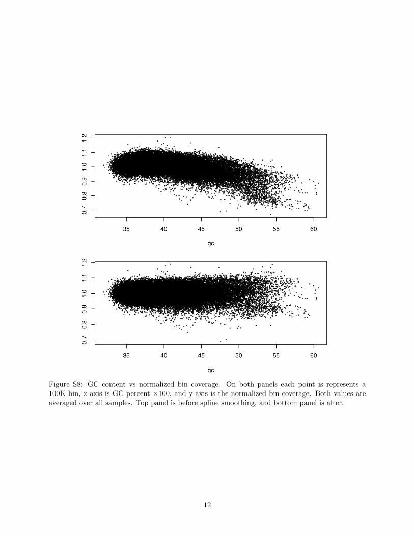
Figure S8: GC content vs normalized bin coverage. On both panels each point is represents a100K bin, x-axis is GC percent ⇥100, and y-axis is the normalized bin coverage. Both values areaveraged over all samples. Top panel is before spline smoothing, and bottom panel is after.

12