infrasound propagation in the “zone of...

Seismological Research Letters Volume 81, Number 4 July/August 2010 615doi: 10.1785/gssrl.81.4.615

Infrasound Propagation in the “Zone of Silence”Petru T. Negraru, Paul Golden, and Eugene T. Herrin

Petru T. Negraru, Paul Golden, and Eugene T. Herrin Southern Methodist University

INTRODUCTION

The speed of sound in an ideal gas, under adiabatic conditions, is a function of temperature and is given by:

C = gRT

where C is the speed of sound, g, known as the adiabatic index, is the ratio of specific heats at constant pressure and constant volume (Cp/Cv), R is the gas constant, and T is the absolute temperature.

In addition to temperature, which is the dominant factor, infrasound propagation is affected by the local wind velocity. Therefore we can combine the temperature and wind effect in the effective sound speed, written as

C eff = C + η⋅υ ,

where Ceff is the effective sound speed, υ is the wind velocity, and η is a unit vector in a direction of sound propagation.

The temperature (and therefore Ceff) distribution in the atmosphere is controlled by solar radiation. As most of the heat transfer takes place on the ground surface, temperature tends to decrease with altitude. A perturbation of this trend occurs in the stratosphere due to the heating associated with absorption of ultraviolet radiation by the ozone layer (Figure 1), but above the ozone layer the temperature decreases again with altitude up to around 100 km. Above this height, in the thermosphere, the temperature increases with altitude due to direct ultravio-let radiation heating from the sun. Classic ray theory implies that infrasound energy, generated on the surface of the ground and propagating through the atmosphere, must reach a layer of effective sound speed greater than the velocity of sound at the source in order to return to receivers located on the surface of the Earth. Normally, this happens at heights around 110 km, in the thermosphere, and these rays are usually recorded at distances greater than 250 km from the source. The region up to 250 km from the source where no infrasound returns are expected has been called the “zone of silence.” This effect is illustrated in Figure 1.

There are a number of historical examples mentioned in the literature that describe this effect. One of them is an explo-sion at Oppau, Germany, in 1921, one of the worst industrial accidents ever. This explosion is estimated to have had a yield

of 1–2 kt of TNT and produced a crater 100 m wide and 20 m deep (Abelshauser et al. 2004). This is probably one of the first reports of a seismo-acoustic event. Ground motions from two explosions were felt in Heidelberg, approximately 22 km away, followed more than a minute later by the sound wave. No sound was heard in an area 100–200 km from the source, but was heard at distances farther than 200 km (Mitra 1952). The term “zone of silence” was introduced by Gutenberg (1939) in his study of sound waves from a detonation of 5,000 kg of ammunition near Berlin. He found that the sound was heard in zones of concentric rings, separated by zones where there were no reports of observations. He called the first zone of no sound observation the “zone of silence.”

A more recent paper by Jones et al. (2004) discusses the occurrence of the zone of silence in different atmospheric condi-tions from a purely theoretical point of view, and suggests infra-sound is observed when there is an inversion of effective sound speed. There are also reports of infrasound being observed within this zone of silence (Gibbons et al. 2007; McKenna et al. 2008). However, empirical studies in this distance range, up to 300 km from the source, are scarce. Most of the infrasound papers report infrasound signals from particular natural or man-made sources such as explosions (Sorrells et al. 1997; Whitaker et al. 1998), sonic booms (Donn 1978; Le Pichon et al. 2002), earthquakes (Donn and Posmentier 1964; Cook 1971; Kim et al. 2004; Mutschlecner and Whitaker 2005), bolides (ReVelle 1976; ReVelle and Whitaker 1999; Evers and Haak 2001) aurora (Wilson 1969, 1971; Wilson et al. 2005), avalanches (Scott et. al. 2007), volcanic eruptions (Goerke et al. 1965; Garces and Hansen 1998; Johnson et al. 2004), severe weather (Bowman and Bedard 1971; Rind 1980; Olson and Szuberla 2005), and animal vocalizations (Larom et. al. 1997), but the propagation is rarely discussed in depth. Kulichkov (2000) discusses the propagation of infrasound signals at distances up to 300 km, and he argues that partial reflection or scattering due to inho-mogeneities in the stratosphere and mesosphere is responsible for the observed signals. McKenna et al. (2008) analyzed a suite of events in Korea at an estimated distance range of 100–200 km and assumed they were observed because of short-lived (on the basis of a few hours) tropospheric inversion layers in effective sound speed (also called ducts). Unfortunately, in the absence of a travel time analysis (not possible because of the lack of ground truth information, i.e., origin time and location), it is not clear if all the recorded signals were actually signals propagating in tropospheric ducts. Therefore better-controlled experiments are needed to understand the propagation of infrasound sig-

616 Seismological Research Letters Volume 81, Number 4 July/August 2010

nals in the zone of silence. Such experiments were carried out in Nevada in 2006 and 2007. This paper presents the most impor-tant results of those experiments and attempts to assess current infrasound propagation modeling capabilities.

SOURCE AND FIELD EXPERIMENTS

The Nevada Infrasound Array (NVIAR), located near the vil-lage of Mina, Nevada, is a four-channel infrasound array with an aperture of approximately 1 km (Figure 2), embedded in the Nevada Seismic Array (NVAR), a permanent International Monitoring System array. Each infrasound station is equipped with a Chapparel II infrasound sensor with a flat response from 0.1 to 200 Hz. Since the array began operating in December 1998, infrasound arrivals from an ordnance disposal facility approximately 36 km away are recorded on a regular basis. The

site has been dubbed “New Bomb.” On a normal operational day there are a variable number of explosions with a separation of 40–70 seconds. In most cases there are five shots, but in the past we have recorded up to 10 detonations, depending on the nature of the operation. The yields of the explosions range from 2,000 to nearly 4,000 lbs. of mixed ordnance. This repetitive pattern (Figure 2, right) is used as an additional source diag-nostic tool because the time interval between the shots is simi-lar no matter where the observations are. Therefore if signals spaced at the right interval are observed, they are likely to be from New Bomb if the azimuth is also correct.

Field experiments to investigate the propagation of infra-sonic waves in the zone of silence were carried out in the summers of 2006 and 2007. In addition to NVIAR data we deployed temporary arrays located in a line north of the source (Figure 3), ranging in distance from 76 to 288 km. In 2006 we

0 100 200 300 400 500 600Range (km)

250 300 350 400 450 500 5500

50

100

150

Effect. Sound Speed along G.C. Path (m/s)

Hei

ght (

km)

Troposphere

Stratosphere

Mesosphere

Thermosphere

ZONE OF SILENCE

▲ Figure 1. Generalized atmospheric propagation model (left) and corresponding rays (right).

NVI01

NVI04

NVI02

NVI03

1000 m

NVAR

New Bomb

Hawthorne Army

Ammunition Depot

▲ Figure 2. Landsat image showing the location of NVAR and the configuration of the NVIAR (left). The plot on the right shows typical signals from the detonation.

Seismological Research Letters Volume 81, Number 4 July/August 2010 617

deployed three temporary arrays at distances of 76, 108, and 157 km due north from the source. The arrays were located in the village of Shurz, Nevada, and north and south of the city of Fallon, Nevada. Accordingly the arrays were called SHURZ (76 km from the source), FALS (108 km), and FALN (157 km). In 2007 we reoccupied the site FALN and deployed an addi-tional array north of Gerlach, Nevada, at a distance of 288 km (called GERL). The temporary arrays had four elements each, deployed in a line toward the source, with an overall aperture of 400 m. The deployment was chosen so that the time lags of the arrivals were maximized, and because we want to be able to conduct future investigations on the infrasound signal and noise correlation. In addition we had excellent cooperation with the officials in charge of the disposal facility, and they released the detonation logs with approximate origin time and yields of the explosions.

We employed the National Severe Storms Laboratory (NSSL) to collect balloon-launched rawinsonde meteorologi-cal data during our field experiments. The rawinsondes col-

lected temperature, dew point, relative humidity, barometric pressure, GPS latitude and longitude, altitude, and wind direc-tion and velocity data. The meteorological data were recorded on an hourly basis at the Hawthorne airport in the path of the propagating signals, from approximately two hours before the detonations to a few hours after the detonations. All meteoro-logical observations range from ground level to the base of the stratosphere, and some of them have maximum heights around 30 km. There is, however, uncertainty in the wind measure-ments taken close to the surface of the Earth (Negraru and Herrin 2009).

METHODOLOGY AND DATA

Accurate origin times for the detonations were obtained from GPS time synchronized video recordings. This allowed us to calibrate the seismic travel time between source and various NVAR channels. Origin times for the detonations without video recordings were obtained from this calibrated seismic

NV02

NV01 NV03

NV04

1000 m

Site 1

Site 2

Site 3

Site 4

50 m

FALN

FALS

SHURZ

NEW BOMBNEW BOMB

NVIAR

GERL

2007 only2006 and 2007

Source

2006 only

▲ Figure 3. Satellite imagery of the area where the temporary arrays were deployed with plan layouts for each of them.


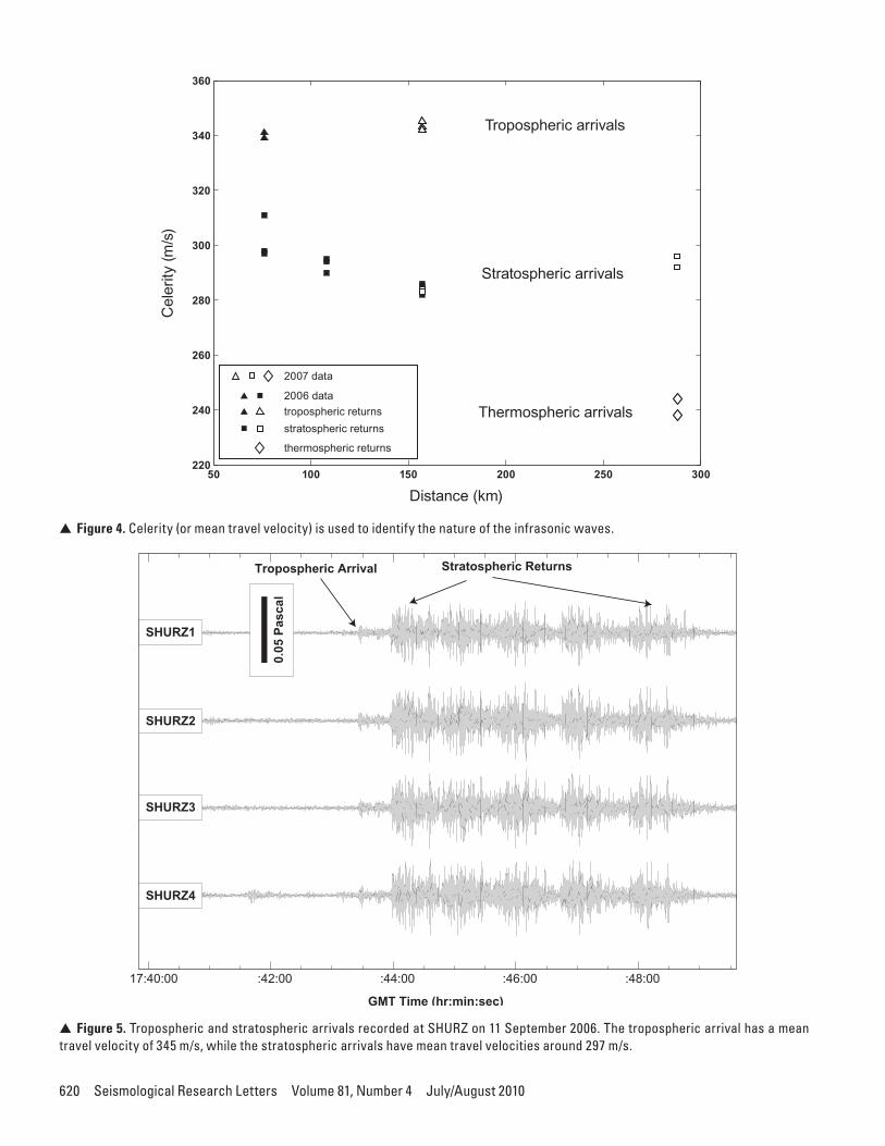
travel time. We believe the origin times to be accurate to within a fraction of a second. This precision is much better than what is needed to compute the mean travel time velocities (also called celerity) for the infrasound arrivals. The celerity is defined as the distance divided by the total travel time, similar to the defi-nition of group velocity for dispersed seismic waves. Tables 1 and 2 gives the origin times, travel times, celerity, and phase velocity of the observed arrivals for 2006 and 2007, respec-tively. The celerity (Figure 4) was used to identify the nature of the infrasonic arrival (Kulichkov et al. 2000). Typically mean travel velocities higher than 330 m/s are found for “boundary layer arrivals” with reflection heights up to 1 km. Tropospheric arrivals are arrivals with reflection heights up to 20 km and have celerities of 310–330 m/s. Stratospheric arrivals have reflection heights of 20–50 km and celerities of 280–320 m/s, while the thermospheric arrivals have celerities of 180–300 m/s (all these values are from Kulichkov 2000). These celerity boundaries are not very well defined, and they could further be affected by seasonal variations. Therefore any interpretation needs to take into account the local atmospheric conditions. Most of the arrivals observed at our arrays have celerities of 280–300 m/s, consistent with stratospheric arrivals. Some of the arrivals have

high celerity values (around 345 m/s), which are consistent with boundary layer arrivals. Throughout the paper we will refer to these arrivals as tropospheric arrivals. The array farthest from the source, at 288 km, recorded arrivals with celerities around 240 m/s, which suggests they have turning points (reflection heights) in the thermosphere or very high in the stratosphere.

Figures 5–8 show various types of arrivals recorded during the experiments. Figure 5 shows tropospheric and stratospheric arrivals recorded at SHURZ (76 km from the source). A signal approximately 30 seconds before the five-shot pattern is inter-preted as a tropospheric arrival from the first detonation. The tropospheric arrivals from the other four detonations are masked by the much larger amplitude of the stratospheric arrivals.

In 2006 tropospheric arrivals were recorded only out to SHURZ (76 km from the source), but in 2007 tropospheric arrivals were recorded at FALN (Figure 6) at a distance of 157 km. Stratospheric arrivals (celerities around 285 m/s) were also observed, except for the last day of the 2007 experiment, when only tropospheric arrivals were observed. The array at GERL observed both stratospheric (celerities 292 m/s) and thermospheric arrivals (celerities around 240 m/s). Shown in Figure 7 is the five-shot pattern observed at NVIAR (upper

TABLE 1Travel Time Analysis for the 2006 Dataset

2006 Experiment 11 September 2 September 13 September

Origin Time17:39:44.2 17:52:26.2 20:49:04.8

Acoustic Arrival Times NVAR (NV03) 17:41:31.0 17:54:12.7 20:50:50.9 SHURZ* 17:43:25.8 17:56:09.3 Not observed SHURZ 17:43:58.7 17:56:39.8 20:53:07.3 FALS 17:45:49.8 17:58:30.0 20:55:19.0 FALN 17:48:54.2 18:01:33.3 20:58:20.2Acoustic Travel Times (seconds) NVAR (NV03) 106.8 106.5 106.1 SHURZ* 221.6 223.1 Not observed SHURZ 254.5 253.6 243.5 FALS 365.6 363.8 371.2 FALN 550.0 547.1 555.4Mean Travel Velocity (m/sec) NVAR (NV03) 344.9 345.9 347.2 SHURZ* 341.3 339.0 Not observed SHURZ 297.1 298.2 310.6 FALS 293.9 295.4 289.5 FALN 284.5 286.0 281.7Phase Velocity (m/sec) NVAR 345 345 345 SHURZ* 349 347 Not observed SHURZ 353 353 352FALS 352 346 358FALN 360 361 356


two waveforms) shifted in time and aligned with the strato-spheric and thermospheric arrivals observed later at Gerlach (lower four waveforms). This time interval among the shots helps discriminate the New Bomb signals from other sources and helps identify the type of arrivals. Due to higher noise lev-els around the time when the last two thermospheric arrivals are expected, they are harder to identify. However, the pattern recognition method is more precise than any other approach we attempted, including the frequency content of the signals. First, any Fourier analysis should be regarded only qualita-tively, as there is no accepted atmospheric absorption model. If we introduce the existing theoretical absorption models (Sutherland and Bass 2004) in the propagation calculations, no thermospheric arrivals should be observed (McKenna et al. 2007). Second, the Fourier analysis has a poor resolution in the frequency domain because of the short time duration of the signals (Figure 8). The stratospheric signals shown in Figure 8 last for at least five seconds, and the corresponding magnitude spectrum shows a sharp decrease in energy above 3 Hz. In con-trast, the thermospheric signals last for about two seconds. The corner in the spectrum is around 1.5 Hz, and it appears that the thermospheric signals have less high-frequency energy than the

stratospheric signals, exactly as expected. An alternative way to investigate the spectrum of the signals is to use an autoregres-sive (AR) method. The AR is a parametric method in which the spectral characteristics are calculated from a polynomial model instead of the signal itself, as in Fourier methods. Presenting the details of the technique is beyond the scope of the present paper, but we refer the interested reader to the work of Priestly (1981). The method has numerous applications in time series analysis and has many applications in other fields. The main difficulty in the AR method is selecting the order of the model. The higher the order, the closer the spectrum representation is, but the spectrum is harder to interpret because of the larger number of spectral peaks. In most cases the order of the model is chosen empirically, so that you have the lowest possible order without losing critical information. To select the optimum order we have gradually increased the order of estimate, and we found that the best representation of the spectrum is obtained with an AR(10) (order 10). The AR spectrum is significantly smoother than the Fourier spectrum and shows that the strato-spheric signals have more energy in 2–4 Hz band when com-pared to the thermospheric signals (Figure 8).

TABLE 2Travel time analysis for the 2007 experiment

2007 Experiment 10 September 11 September 12 September 13 September

Origin Time17:41:20.3 17:30:40.8 17:35:24.7 17:41:06.6

Acoustic Arrival Time NV03 17:43:07.4 17:32:27.1 17:37:10.4 17:42:53.2 FALN* Not operating 17:38:16.4 17:42:58.0 17:48:44.7 FALN Not operating 17:39:49.2 17:44:35.3 17:50:18.8 GERL 17:57:44.8 Not observed 17:51:35.7 Not observed GERLT 18:00:57.3 Not observed 17:55:35.7 Not observedAcoustic Travel Time (seconds) NV03 107.1 106.3 105.7 106.2 FALN* Not operating 455.6 453.3 458.1 FALN Not operating 549.2 550.6 Not observed GERL 984.5 Not observed 971 Not observed GERLT 1177 Not observed 1211 Not observedMean Travel Velocity (m/s) NV03 344 346 348 347 FALN* Not operating 343 345 342 FALN Not operating 286 284 Not observed GERL 292.1 Not observed 296 Not observed GERLT 244 Not observed 238 Not observedPhase Velocity (m/s) NVAR 346 352 354 356 FALN* Not operating 345 352 355 FALN Not operating 352 358 Not observed GERL 358 Not observed 360 Not observed GERLT 415 Not observed 353 Not observed


50 100 150 200 250 300220

240

260

280

300

320

340

360

Distance (km)

Cel

erity

(m/s

)

2007 data

2006 datatropospheric returnsstratospheric returns

thermospheric returns

Tropospheric arrivals

Stratospheric arrivals

Thermospheric arrivals

▲ Figure 4. Celerity (or mean travel velocity) is used to identify the nature of the infrasonic waves.

0

0

0

17:40:00 :42:00 :44:00 :46:00 :48:00

GMT Time (hr:min:sec)

SHURZ1

SHURZ3

SHURZ2

SHURZ4

0.05

Pas

cal

Tropospheric Arrival Stratospheric Returns

▲ Figure 5. Tropospheric and stratospheric arrivals recorded at SHURZ on 11 September 2006. The tropospheric arrival has a mean travel velocity of 345 m/s, while the stratospheric arrivals have mean travel velocities around 297 m/s.


0FALN01

0FALN02

0FALN03

0FALN04

17:42:00 :44:00 :46:00 :48:00 :50:00

Time (hr:min:sec)

0.2

Pasc

als

First tropospheric signal

First stratospheric signal

Tropospheric and stratospheric interference

▲ Figure 6. Tropospheric and stratospheric signals recorded at FALN on 12 September 2007 (157 km from the source).

▲ Figure 7. Explosion pattern at NVIAR (upper two waveforms) shifted in time so that it aligns with the stratospheric and thermo-spheric arrivals recorded at GERL on 10 September 2007 (288 km from the source).


MODELING

We have used the Naval Research Laboratory Ground to Space (NRL-G2S) atmospheric model (Drob 2004) and direct meteorological observations as the starting point. The NRL-G2S is a semi-empirical hybrid model, obtained from clima-tologies and numerical weather predictions. Above 50 km the G2S is based on the Mass Spectrometer and Incoherent Radar Model (MSIS-90; Hedin 1991 and Picone et al. 2002) and the Horizontal Wind Model (HWM-93; Hedin et al. 1996). The MSIS-90 and HWM-93 are obtained from a 40-year histori-cal database of upper atmosphere measurements and provide a good estimate of the mean winds and temperatures in the mesosphere and lower thermosphere, but the vertical resolu-tion of 1–2 km limits the use of these models below 50 km. Above 50 km the NRL-G2S is based on the numerical weather predictions. The NRL-G2S model provides the atmospheric specifications in a single binary coefficient every six hours, with a delay of a few hours.

The G2S files are fully integrated in InfraMAP (Gibson and Norris 2004), the atmospheric propagation code we have used for modeling. We have used the parabolic equation code

(PE), which is a parabolic approximation to the wave equation. The PE calculations provide an amplitude field at each height (altitude) and range (distance) for a particular frequency. The mathematical details of the PE code implementation can be found in West et al. (1992) and Jensen et al. (1994).

The pressure field calculations are relatively similar if we use the G2S model for 2006 or 2007; therefore we show only the output for the 2007 dataset (upper plot, Figure 9). Also shown in the figure are the locations of the temporary arrays deployed during the experiments. It is clear that the G2S model does not explain the recorded stratospheric arrivals that occur at all arrays (with the exception of NVIAR, which is too close). Thermospheric arrivals are recorded at GERL at a distance of 288 km, while the energy is predicted to return at distances larger than 300 km. Tropospheric arrivals may be predicted at SHURZ but not at FALN.

Apart from the G2S model we have used the actual meteo-rological data acquired at the Hawthorne airport. The PE cal-culations for the 2007 experiment (lower plot, Figure 9) show the presence of a low-velocity layer, approximately 100 meters thick, which is capable of trapping the energy and explains the tropospheric arrivals recorded at FALN. It should be noted that

10-1 100 101 102100

90

80

70

60

50

40

30

20

Frequency (Hertz)

PSD

(dB

rela

tive

to P

asca

l2 /Hz2 )

AR10 for stratospehric and thermospheric signals

stratosphericthermospheric

100 101

10-3

10�-2

10�-1

100

Frequency (Hertz)

Mag

nitu

de

Fourier Transform

stratosphericthermospheric

�

�

�

�

stratospheric

thermospheric

Pres

sure

(Pas

cals

)

Time (seconds)0 864 5 71 2 3

-0.2

-0.1

00.050.1

0.15

-0.15

-0.05

-0.2

-0.1

00.050.1

0.15

-0.15

-0.05

▲ Figure 8. Observed stratospheric and thermospheric arrivals at Gerlach for 10 September 2009 (upper plot) and corresponding Fourier (lower left) and AR (lower right) spectra.


if we use a different atmospheric profile, obtained a few hours after the detonations, there is no duct capable of trapping energy. This fact could explain why the G2S model, which is a six-hour average, did not predict tropospheric arrivals. These short-lived atmospheric ducts were previously reported by McKenna et al. (2008), but it appears that these ducts could have a life shorter than two hours, perhaps even a few tens of minutes.

DISCUSSION

Very precise ground truth information on a repetitive source allowed us to make a reliable travel time analysis, which holds the key in correctly identifying the nature of the observed

infrasound arrival. Overall, stratospheric signals appear to be the dominant type of arrival in the zone of silence, but they are not predicted by current models. Tropospheric sig-nals were recorded up to distances of 156 km, but they may very well be observed at greater distances depending on the nature of the inversion layer. These arrivals are predicted by the current modeling information if local meteorological data is used as input in the modeling codes. The life of these inver-sion layers could be very short, probably even shorter than an hour. Future G2S models will provide mesoscale specifications on an average of one hour for the continental United States (Doug Drob, personal communication, 2008). It is possible that these future specifications might have the necessary time

Range (km)

Hei

ght (

km)

0 50 100 150 200 250 300 350 4000

20

40

60

80

100

120

140

100

90

80

70

60

50

40

30

20

10

0

250 300 350 400 450 5000

20

40

60

80

100

120

140

Effective Sound Speed along the path (m/s)

Hei

ght (

km)

PE without absorption for 2007 data (2 Hz). Amplitude field is in dB.

Naval Research Lab. Ground to Space Modelfor 09/12/2007.

GERLFALN

Range (km)

Hei

ght (

km)

0 50 100 150 200 2500

5

10

15

100

90

80

70

60

50

40

30

20

10

0

GERLFALN

280 290 300 310 320 330 340 3500

5

10

15

Effective Sound Speed (m/s)

Hei

ght (

km)

PE without absorption for 2007 data (2 Hz). Amplitude field is in dB.

Local meterological aquired in the path of the propagating signals on 09/12/2007.

SHURZ FALS

▲ Figure 9. NRL-G2S atmospheric model (upper figure left) for 12 September 2007, and corresponding pressure field (upper figure right) obtained using a parabolic approximation to the wave equation. Lower plot shows the atmospheric profile obtained from direct meteorological observations (left) and pressure field (right).


resolution to accurately predict the tropospheric and strato-spheric arrivals.

An interesting problem usually not mentioned in the lit-erature is the link between phase velocity and celerity. Figure 10 shows the observed signals at FALN on 13 September 2006. This was the last day of the 2006 experiment, with only four explosions. For each explosion there are at least four individual arrivals, and the phase velocity is increasing while celerity decreases. All these arrivals have celerities consistent with stratospheric arrivals and suggest the presence of a lay-ered structure in the stratosphere with effective sound speed increasing with height. However, in infrasound monitoring, the origin time and source location (and eventually yield) of an infrasound event is usually the scope of the investigation and they are not known a priori. Therefore the celerity is very difficult to estimate, and any useful information needs to be extracted from the phase velocity and azimuth. Our data shows that similar phase velocities can be obtained for a very large range of celerities (from 0.345 to 0.240), indicating that it is difficult to infer the nature of the infrasound from phase veloc-ities only. The relationship of fast phase velocity/slow celerity is in general valid, but there can be exceptions. The arrivals hav-ing phase velocities in excess of 370 m/s are very unlikely to be

observed for tropospheric arrivals, but phase velocities around 345–355 m/s were observed occasionally for all types of arriv-als (tropospheric, stratospheric, and thermospheric), suggesting that the atmospheric temporal variability (particularly local winds at the array) could play an important role.

ACKNOWLEDGMENTS

The authors would like to thank to Rodney Whitaker from Los Alamos National Laboratory for help with interpretation, Douglas Drob from Naval Research Laboratory for providing the G2S models, and Suzanne Lehr from the Ammunition Depot in Hawthorne for ground truth information.

REFERENCES

Abelshauser, W., W. von Hippel, J. A. Johnson, and R. G. Stokes (2004). German Industry and Global Enterprise: BASF: The History of a Company. Cambridge and New York: Cambridge University Press.

Bowman, H. S., and A. J. Bedard (1971). Observations of infrasound and subsonic disturbances related to severe weather. Geophysical Journal of the Royal Astronomical Society 26, 215–242.

Cook, K. R. (1971). Infrasound radiated during the Montana earthquake of 1959 August 18. Geophysical Journal of the Royal Astronomical Society 26, 191–198.

0

0

0

20:58:00 21:00:00 21:02:00

0.2

Pasc

als

FALN 04

FALN 01

FALN 02

FALN 03

GMT Time

Mean Travel Velocity 277Phase Velocity 359



▲ Figure 10. FALN observations for the last day of the 2006 experiment (13 September) showing multiple stratospheric impulsive arriv-als. Also shown are the celerity and the phase velocity for individual arrivals.


Donn, W. L. (1978). Exploring the atmosphere with sonic booms. American Scientist 66, 724–733.

Donn, W. L., and E. S. Posmentier (1964). Ground-coupled air waves from the great Alaskan earthquake. Journal of Geophysical Research 69, 5,357–5,361

Drob, D. P. (2004). Atmospheric specifications for infrasound calcula-tions. Inframatics 5, 1–13.

Evers, L. G., and H. W. Haak (2001). Listening to sounds from an exploding meteor and oceanic waves. Geophysical Research Letters 28 (1), 41–44.

Garces, M. A., and R. A. Hansen (1998). Waveform analysis of seismoa-coustic signals radiated during the fall 1996 eruption of Pavlof vol-cano, Alaska. Journal of Geophysical Research 25 (7), 1,051–1,054.

Gibbons, S. J., F. Ringdal, and T. Kvaerna (2007). Joint seismic-infra-sonic processing of recordings from a repeating source of atmo-spheric explosions. Journal of the Acoustical Society of America 122 (5), EL158– EL164.

Gibson, R., and D. Norris (2004). Integration of infrasound propaga-tion models and near-real-time atmospheric characterizations. Proceedings of the 26th Seismic Research Review: Trends in Nuclear Explosion Monitoring, Los Angeles Technical Report LA-UR-04-5801 2, 635–644.

Goerke, V. Y., and R. Cook (1965). Infrasonic observation of the May 14, 1963 volcanic explosion on the Island of Bali. Journal of Geophysical Research 70, 6,017–6,022.

Gutenberg, B. (1939). The velocity of sound waves and the temperature in the stratosphere in southern California. Bulletin of the American Meteorological Society 20, 192–201.

Hedin, A. E. (1991). Extension of the MSIS thermosphere model into the middle and lower atmosphere. Journal of Geophysical Research 96, 1,159–1,172.

Hedin, A. E., E. L. Fleming, A. H. Manson, F. J. Schmidlin, S. K. Avery, R. R. Clark, S. J. Franke, G. J. Fraser, T. Tsuda, F. Vial, and R. A. Vincent (1996). Empirical wind model for the upper, middle and lower atmosphere. Journal of Atmospheric and Terrestrial Physics 58, 1,421–1,447; doi:10.1016/0021-9169(95)00122-0.

Jensen, F. B., W. A. Kuperman, M. B. Porter, and H. Schmidt (1994). Computational Ocean Acoustics. New York: AIP Press.

Johnson, J. B., R. C. Aster, and P. R. Kyle (2004). Volcanic eruptions observed with infrasound. Geophysical Research Letters 31, L14604; doi:10.1029/2004GL020020.

Jones, R. M., E. S. Gu, and A. J. Bedard Jr. (2004). Infrasonic atmospheric propagation studies using a 3-D ray trace model. In Proceedings of the 22nd Conference on Severe Local Storms, Hyannis, MA, 4–8 October P29, American Meteorological Society.

Kim, T. S., C. Hayward, and B. Stump (2004). Local infrasound signals from the Tokachi-Oki earthquake. Geophysical Research Letters 31, L20605, doi:10.1029/2004GL021178.

Kulichkov, S. N. (2000). On infrasonic arrivals in the zone of geometric shadow at long distances from surface explosions. In Proceedings of the Ninth Annual Symposium on Long-Range Propagation, Oxford, MS, 14–15 September, 238–251. National Center for Physical Acoustics.

Kulichkov, S. N., D. O. ReVelle, R. W. Whitaker, and O. M. Raspopov (2000). On so-called “tropospheric” arrivals at long distances from surface explosions. In Proceedings of the Ninth Annual Symposium on Long-Range Propagation, Oxford, MS, September 14–15, 229–237. National Center for Physical Acoustics.

Larom, D., M. Garstang, K. Payne, R. Raspet, and M. Lindeque (1997). The influence of surface atmospheric conditions on the range and area reached by animal vocalizations. Journal of Experimental Biology 200, 421–431.

Le Pichon, A., M. Garces, E. Blanc, M. Barthelemy, and D. P. Drob (2002). Atmospheric characteristics from waves from Concorde. Journal of the Acoustical Society of America 111 (1), Part 2, 629–641.

McKenna, M. H., B. W. Stump, S. Hayek, J. R. McKenna and T. R. Stanton (2007). Tele-infrasonic studies of hard-rock mining explo-sions. Journal of the Acoustical Society of America 122 (1), 97–106.

McKenna, M. H., B. W. Stump, and C. Hayward (2008). Effect of time-varying tropospheric models on near-regional and regional infra-sound propagation as constrained by observational data. Journal of Geophysical Research 113, D11111; doi:10.1029/2007JD009130.

Mitra, S. K. (1952). The Upper Atmosphere. Calcutta: Asiatic Society, 713 pps.

Mutschlecner, J. P., and R. W. Whitaker (2005). Infrasound from earthquakes. Journal of Geophysical Research 110, D01108; doi:10.1029/2004JD005067.

Negraru, P. T., and E. T. Herrin (2009). On infrasound waveguides and dispersion. Seismological Research Letters 80 (4), 565–571; doi:10.1785/gssrl.81.4.565.

Olson, J. V., and C. A. L. Szuberla (2005). Distribution of wave packet sizes in microbarom wave trains observed in Alaska. Journal of the Acoustical Society of America 117, 1,032–1,037.

Picone, J. M., A. E. Hedin, D. P. Drob, and A. C. Aikin (2002). NRLMSISE-00 empirical model of the atmosphere: Statistical comparisons and scientific issues. Journal of Geophysical Research 107(A12), 1,468; doi:10.1029/2002JA009430.

Priestley, M. B. (1981). Spectral analysis and time series. New York: Academic Press.

ReVelle, D. O. (1976). On meteor generated infrasound. Journal of Geophysical Research 81 (7), 1,217–1,230.

ReVelle, D. O., and R W. Whitaker (1999). Infrasonic detection of a Leonid bolide: 1998 November 17. Meteoritics and Planetary Science 34, 995–1,005.

Rind, D. (1980). Microseism at Palisades. Journal of Geophysical Research 85, 4,854–4,862.

Scott, E. D., C. T. Hayward, R. F. Kubichek, J. C. Hamann, J. W. Pierre, B. Comey, and T. Mendenhall (2007). Single and multiple sensor identification of avalanche-generated infrasound. Cold Regions Science and Technology 47 (1–2), 159–170.

Sorrells, G., E. T. Herrin, and J. L. Bonner (1997). Construction of regional ground truth databases using seismic and infrasound data. Seismological Research Letters 68, 743–752.

Sutherland, L., and H. Bass (2004). Atmospheric absorption in the atmo-sphere up to 160 km. Journal of the Acoustical Society of America 115, 1,021–1,032; doi:10.1121/1.161937

West, M., K. E. Gilbert, and R. A. Sack (1992). A tutorial on the para-bolic equation (PE) model used for long range propagation in the atmosphere. Applied Acoustics 37, 31–49.

Whitaker, R.W., J. P. Mutschlecner, M. B. Davidson, and S. D. Noel (1998). Infrasonic Observations of Large-scale HE Events. Los Alamos Technical Report, LA-UR-90-1998.

Wilson, C. R. (1969). Auroral infrasonic waves. Journal of Geophysical Research 78, 1,812–1,826.

Wilson, C. R. (1971). Auroral infrasonic waves and poleward expan-sion of auroral substorms in Inuvik, N.W.T., Canada. Geophysical Journal of the Royal Astronomical Society 26, 179–181.

Wilson, C. R., J. V. Olson, and H. C. Stenbaek-Nielsen (2005). High trace-velocity infrasound from pulsating auroras at Fairbanks, Alaska. Geophysical Research Letters 32, L14810; doi:10.1029/2005GL023188.

Southern Methodist UniversityP.O. Box 750395

Dallas, Texas 75206 [email protected]

(P. T. N.)

infrasound propagation in the “zone of...

Documents