inférence des déplacements humains sur un réseau de ... thanks to telecommunication advancement,...
TRANSCRIPT

Thése de doctorat conjointtelecom sudparis et l’universite Pierre et Marie
Curie
Présentée Par:
Fereshteh ASGARI
Pour obtenir le grade de
DOCTEUR DE TELECOM SUDPARIS
Spécialité: Informatique et Télécommunication
Inférence des déplacements humains sur unréseau de transport multimodal par l’analyse des
meta-données d’un réseau mobile
Soutenue le: 30/03/2016 devant le jury composé de:
Mr. Ken CHEN Université Paris 13 Rapporteur
Mr. Marco FIORE Politecnico of Torino, CNR Rapporteur
Mr. Miguel NUNEZ Université du Pacifique Examinateur
Mr. Hossam AFIFI Telecom SudParis Examinateur
Mr. Nicolas GAUDE Bouygues Telecom Examinateur
Ms. Monique BECKER Telecom SudParis Directrice de Thése
Mr. Mounim EL-YACOUBI Telecom SudParis Co-Directeur de Thése
Mr. Vincent GAUTHIER Telecom SudParis Encadrant de Thése
Thése n◦: 2016TELE0005


JOINT DOCTORATE OF
TELECOM SUDPARIS and UNIVERSITY OF PIERRE & MARIE CURIE
Presented by:
Fereshteh ASGARI
For the degree of
Doctorate of Telecom SudParus
Inferring User Multimodal Trajectories fromCellular Network Metadata in Metropolitan
Areas
Thesis Defense Data: 30/03/2016
Mr. Ken CHEN Université Paris 13 Reviewer
Mr. Marco FIORE Politecnico of Torino, CNR Reviewer
Mr. Miguel NUNEZ Université du Pacifique Examinator
Mr. Hossam AFIFI Telecom SudParis Examinateur
Mr. Nicolas GAUDE Bouygues Telecom Examinator
Ms. Monique BECKER Telecom SudParis Thesis Director
Mr. Mounim EL-YACOUBI Telecom SudParis Thesis Co-director
Mr. Vincent GAUTHIER Telecom SudParis Thesis Superviseor
Thesis number: 2016TELE0005

ii

"The science of today is the technology of tomorrow."
Edward Teller


AbstractAround half of the world’s population are living in cities where different transporta-
tion networks are cooperating together to provide efficient transportation facilities for
individuals. To improve the performance of the multimodal transportation network
it is crucial to monitor and analysis the multimodal trajectories. However obtaining
the multimodal mobility data is not a trivial task. GPS data with fine accuracy, is
extremely expensive to collect; Additionally, GPS is not available in tunnels and un-
derground. Recently, thanks to telecommunication advancement, cellular data used as
Call Data Records (CDRs), is great resource of mobility data, nevertheless it is noisy
and sparse in time; Subsequently it is not a proper resource for multimodal mobility
data in metropolitan areas. The objective the present thesis is to propose a solution to
this challenging issue of inferring real trajectory and transportation layer from wholly
cellular observations. To achieve these objectives we use Cellular signalization data
which is more frequent than CDRs and despite their spatial inaccuracy, they provide
a fair source of multimodal trajectory data. We propose ’CT-Mapper’ to map cellular
signalization data collected from smart phones over the multimodal transportation
network. The proposed algorithm uses Hidden Markov Model property and topolog-
ical properties of different transportation layers to model an unsupervised mapping
algorithm which maps sparse cellular trajectories on multilayer transportation net-
work. Later on, we propose LCT-Mapper an algorithm to infer the main mode of
trajectories. The area of study in this research work is Paris and its suburbs (Ile-de-
France); we have modeled and built the multimodal transportation network database.
To evaluate our proposed algorithms we use real trajectories data sets collected from a
group of volunteers over a period of one month. Users’ cellular signalization data was
provided by a french operator to assess the performance of our proposed algorithms
using GPS data as ground truth. An extensive set of evaluations has been performed
to validate the proposed algorithms. To summarize, it is shown in this work that
it is feasible to infer the multimodal trajectory of users in an unsupervised manner.
Our achievement makes it possible to investigate the multimodal mobility behavior
of people and explore and monitor the population flow over multilayer transportation

network.
Keywords: Multimodal trajectory - Cellular signalization data - Cellular trajectory-
Trajectory mapping - Multilayer transportation network- Mode Inference

AbstractDans cette thèse, nous avons étudier une méthode de classification et d’évaluation des
modalités de transport utilisées par les porteurs de mobile durant leurs trajets quo-
tidiens. Les informations de mobilité sont collectées par un opérateur au travers des
logs du réseau téléphonique mobile qui fournissent des informations sur les stations
de base qui ont été utilisées par un mobile durant son trajet. Les signaux (appel-
s/SMS/3G/4G) émis par les téléphones sont une source dinformation pertinente pour
l’analyse de la mobilité humaine, mais au-delà de ça, ces données représentent surtout
un moyen de caractériser les habitudes et les comportements humains. Bien que
l’analyse des metadata permette dacquérir des informations spatio-temporelles à une
échelle sans précédent, ces données présentent aussi de nombreuses problématiques à
traiter afin den extraire une information pertinente.
Notre objectif dans cette thèse est de proposer une solution au problème de déduire
la trajectoire réelle sur des réseaux de transport à partir dobservations de position
obtenues grâce à l’analyse de la signalisation sur les réseaux cellulaires. Nous pro-
posons "CT-Mapper" pour projecter les données de signalisation cellulaires recueillies
auprès de smartphone sur le réseau de transport multimodal. Notre algorithme utilise
un modèle de Markov caché et les propriétés topologiques des différentes couches de
transport. Ensuite, nous proposons "LCT-Mapper" un algorithme qui permet de
déduire le mode de transport utilisé.
Pour évaluer nos algorithmes, nous avons reconstruit les réseaux de transport de
Paris et de la région (Ile-de-France). Puis nous avons collecté un jeu de données de
trajectoires réelles recueillies auprès dun groupe de volontaires pendant une période
de 1 mois. Les données de signalisation cellulaire de l’utilisateur ont été fournies par
un opérateur français pour évaluer les performances de nos algorithmes à l’aide de
données GPS.
Pour conclure, nous avons montré dans ce travail qu’il est possible d’en déduire la tra-
jectoire multimodale des utilisateurs d’une manière non supervisée. Notre réalisation

permet d’étudier le comportement de mobilité multimodale de personnes et d’explorer
et de contrôler le flux de la population sur le réseau de transport multicouche.
Mots-clés : trajectoires multimodal - données de signalisation cellulaire - cartographie
trajectoire- Trajectoire cellulaire - transport multicouche de mode Inférence.

"We only have what we give."
Isabel Allende
AcknowledgementsI would like to thank my two supervisors: Vincent Gauthier and Mounim El Yacoubi
whom without their help and guidance this thesis would have not been possible. Vin-
cent helped me through this PhD work and updated me with new studies and works.
I also thank him for providing me the possibility to experience a research visit during
my PhD work. I thank Mounim for his help and constructive comments and guidance
during this work. His clear detailed critics always helped me improve my work and
look for solutions in the right place. He provided many suggestions to improve the
readability of different versions of the present.
I would then like to thank Prof. Monique Becker for her scientific guidance and sup-
port, but also for her kindness. I thank her for the trust she had in me to do this
research. I have learnt to improve my work from her and her feedback and patience
have always helped all along this journey.
I wish to thank Prof. Marco Fiore, Prof. Ken Chen, Prof. Harvé Debar, Dr. Miguel
Nunez and Mr. Nicolas Gaude for having served as my committee members.
My special thanks to Prof. Hakima Chauchi, EIT Digital Paris coordinator for her
helps and supports for the research visit during my PhD study. I would like to thank
Prof. Alex Arenas to host me in his lab, as well as Alberto Sole for his time and
advise during our fruitful discussions and talks.
Then I wish to thank each and every one of my friends and colleagues who helped me
with their participation in data collection.
Then I tend to thank my friends whom their friendship makes the world a better place
for me. Some I have known for many years, some have entered my life more recently.
Some are geographically far but always present and some others have become my
Parisian family.
Last but not least, I am grateful to my family, whose continuous support has encour-
aged me to get this far and to be who I am here present. In the end, my sincere
thanks to the one who stood by me along the last year of this roller coaster ride and
who always embrased me with his love.
Fereshteh Asgari
ix


Contents
Abstract v
Résumé vii
Acknowledgements ix
Table of Contents x
List of Figures xv
List of Tables xvii
Abbreviations xix
1 Introduction 11.1 Motivations and Challenges . . . . . . . . . . . . . . . . . . . . . . . . 31.2 Thesis Contributions . . . . . . . . . . . . . . . . . . . . . . . . . . . . 31.3 Thesis Organization . . . . . . . . . . . . . . . . . . . . . . . . . . . . 5
2 State Of The Art 92.1 Introduction . . . . . . . . . . . . . . . . . . . . . . . . . . . . . . . . . 92.2 General Human Mobility Models . . . . . . . . . . . . . . . . . . . . . 10
2.2.1 Spatial Dimension . . . . . . . . . . . . . . . . . . . . . . . . . 112.2.2 Temporal Dimension . . . . . . . . . . . . . . . . . . . . . . . . 142.2.3 Social Dimension . . . . . . . . . . . . . . . . . . . . . . . . . . 15
2.3 Spatial Networks in Human Mobility . . . . . . . . . . . . . . . . . . . 162.3.1 Centrality Measures . . . . . . . . . . . . . . . . . . . . . . . . 172.3.2 Multimodal Transportation Networks and Complex Networks . 19
2.4 Mobility Data . . . . . . . . . . . . . . . . . . . . . . . . . . . . . . . 202.5 Mapping Algorithms . . . . . . . . . . . . . . . . . . . . . . . . . . . . 23
2.5.1 Hidden Markov Models & Viterbi Algorithm . . . . . . . . . . 232.5.1.1 Viterbi Decoding Algorithm . . . . . . . . . . . . . . . 25
2.6 Conclusion . . . . . . . . . . . . . . . . . . . . . . . . . . . . . . . . . . 27
xi

Contents xii
3 Transportation Network Database and Mobility Datasets 313.1 Introduction . . . . . . . . . . . . . . . . . . . . . . . . . . . . . . . . . 313.2 Multimodal Transportation Graph Databas . . . . . . . . . . . . . . . 33
3.2.1 Multimodal Transportation Graph Representation . . . . . . . 343.2.2 Data Extraction for Network Construction . . . . . . . . . . . . 353.2.3 Multimodal Transportation Network Database . . . . . . . . . 37
3.2.3.1 Data Model . . . . . . . . . . . . . . . . . . . . . . . . 373.2.3.2 Database Model . . . . . . . . . . . . . . . . . . . . . 37
3.2.4 Graph Statistics . . . . . . . . . . . . . . . . . . . . . . . . . . 393.3 Multimodal Cellular Trajectories Dataset . . . . . . . . . . . . . . . . 403.4 Multimodal GPS Trajectories Dataset . . . . . . . . . . . . . . . . . . 423.5 Conclusion . . . . . . . . . . . . . . . . . . . . . . . . . . . . . . . . . . 44
4 Methodology:CT-MapperMapping Sparse Cellular Trajectories to Multimodal TransportationNetwork 474.1 Introduction . . . . . . . . . . . . . . . . . . . . . . . . . . . . . . . . . 474.2 Related Work . . . . . . . . . . . . . . . . . . . . . . . . . . . . . . . . 52
4.2.1 General Human Mobility Models . . . . . . . . . . . . . . . . . 524.2.2 Mapping Algorithms . . . . . . . . . . . . . . . . . . . . . . . . 534.2.3 Human Mobility Modeling with CDR Cellular Trajectories . . . 53
4.3 CT-Mapper System Overview . . . . . . . . . . . . . . . . . . . . . . . 544.3.1 Problem Statement . . . . . . . . . . . . . . . . . . . . . . . . . 544.3.2 Data Collection and Datasets . . . . . . . . . . . . . . . . . . . 564.3.3 Computational Complexity of the Mapping Problem in the Col-
lected Datasets . . . . . . . . . . . . . . . . . . . . . . . . . . . 574.3.4 Framework and Overall Design . . . . . . . . . . . . . . . . . . 59
4.4 Core Algorithms . . . . . . . . . . . . . . . . . . . . . . . . . . . . . . 614.4.1 Transition Probability . . . . . . . . . . . . . . . . . . . . . . . 614.4.2 Emission Probability . . . . . . . . . . . . . . . . . . . . . . . . 64
4.5 Discussion & Conclusion . . . . . . . . . . . . . . . . . . . . . . . . . . 65
5 Mode Classification with LCT-Mapper 675.1 Introduction . . . . . . . . . . . . . . . . . . . . . . . . . . . . . . . . . 675.2 LCT-Mapper System Overview . . . . . . . . . . . . . . . . . . . . . . 71
5.2.1 Problem Statement . . . . . . . . . . . . . . . . . . . . . . . . . 715.2.2 Algorithm Framework . . . . . . . . . . . . . . . . . . . . . . . 72
5.2.2.1 Class-Layer Classifier . . . . . . . . . . . . . . . . . . 735.3 Discussion . . . . . . . . . . . . . . . . . . . . . . . . . . . . . . . . . . 755.4 Conclusion . . . . . . . . . . . . . . . . . . . . . . . . . . . . . . . . . . 75
6 Algorithms Validation 776.1 Introduction . . . . . . . . . . . . . . . . . . . . . . . . . . . . . . . . . 776.2 Metrics For Performance Evaluation . . . . . . . . . . . . . . . . . . . 78
6.2.1 Root Mean Square Error . . . . . . . . . . . . . . . . . . . . . . 78

Contents xiii
6.2.2 Edit Based Similarity Score . . . . . . . . . . . . . . . . . . . . 806.2.3 Recall and Precision . . . . . . . . . . . . . . . . . . . . . . . . 826.2.4 F-Measure . . . . . . . . . . . . . . . . . . . . . . . . . . . . . . 83
6.3 Dataset for Evaluation . . . . . . . . . . . . . . . . . . . . . . . . . . . 836.4 CT-Mapper Evaluation . . . . . . . . . . . . . . . . . . . . . . . . . . . 85
6.4.1 Algorithm Performance . . . . . . . . . . . . . . . . . . . . . . 856.4.2 Comparison with Baseline . . . . . . . . . . . . . . . . . . . . . 866.4.3 Multimodality Analysis . . . . . . . . . . . . . . . . . . . . . . 88
6.5 LCT-Mapper Evaluation . . . . . . . . . . . . . . . . . . . . . . . . . . 896.5.1 Algorithm Performance . . . . . . . . . . . . . . . . . . . . . . 896.5.2 Comparison with Baseline and CT-Mapper . . . . . . . . . . . 906.5.3 Mode Classification . . . . . . . . . . . . . . . . . . . . . . . . . 94
6.6 Discussion & Conclusion . . . . . . . . . . . . . . . . . . . . . . . . . . 95
7 Conclusion 977.1 Contributions . . . . . . . . . . . . . . . . . . . . . . . . . . . . . . . . 977.2 Limitations . . . . . . . . . . . . . . . . . . . . . . . . . . . . . . . . . 987.3 Future Directions . . . . . . . . . . . . . . . . . . . . . . . . . . . . . . 99
Bibliography 101


List of Figures
1.1 An overview of the framework for proposed mapping approch . . . . . 51.2 Chapters classification . . . . . . . . . . . . . . . . . . . . . . . . . . . 6
2.1 Human mobility properties [12] [27] . . . . . . . . . . . . . . . . . . . . . 102.2 viterbi example . . . . . . . . . . . . . . . . . . . . . . . . . . . . . . 27
3.1 Different Data Resources . . . . . . . . . . . . . . . . . . . . . . . . . . 323.2 In station ’Denfert Rochereau’ two metro lines and a train line meet . . . . 333.3 The Multilayer transportation network is obtained by defining cross-
layer links between different transportation layers . . . . . . . . . . . . 343.4 nodes and edges as a document in a document database . . . . . . . . 383.5 Transportation layers . . . . . . . . . . . . . . . . . . . . . . . . . . . . 39
(a) Road . . . . . . . . . . . . . . . . . . . . . . . . . . . . . . . . . 39(b) Train . . . . . . . . . . . . . . . . . . . . . . . . . . . . . . . . . 39(c) Subway . . . . . . . . . . . . . . . . . . . . . . . . . . . . . . . . 39(d) Multilayer . . . . . . . . . . . . . . . . . . . . . . . . . . . . . . 39
3.6 Cellular signalization data of a smartphone user during 100 days in Paris and vicin-ity. Blue circles are the most frequent visited places . . . . . . . . . . . . . . . 41
3.7 Radius of Gyration . . . . . . . . . . . . . . . . . . . . . . . . . . . . . 423.8 An example of multimodal trajectory . . . . . . . . . . . . . . . . . . . 433.9 The coverage area of GPS data collected is shown in yellow on the map
of Paris and region . . . . . . . . . . . . . . . . . . . . . . . . . . . . . 443.10 GPS Trajectoreis Lendth and Time distributions . . . . . . . . . . . . 44
(a) Length distribution . . . . . . . . . . . . . . . . . . . . . . . . . . 44(b) Time distribution . . . . . . . . . . . . . . . . . . . . . . . . . . 44
4.1 Example of mapping algorithm . . . . . . . . . . . . . . . . . . . . . . 49(a) Road Trajectory . . . . . . . . . . . . . . . . . . . . . . . . . . . 49(b) GPS Trajectory . . . . . . . . . . . . . . . . . . . . . . . . . . . . 49(c) Cell Trajectory (Full) . . . . . . . . . . . . . . . . . . . . . . . . 49(d) CDR Trajectory . . . . . . . . . . . . . . . . . . . . . . . . . . . 49(e) Sparse Cell Trajectory . . . . . . . . . . . . . . . . . . . . . . . . 49
4.2 Multilayer representation of different transportation networks . . . . . . . . 554.3 Voronoi tessellation of cellular antennas in Ile-de-France . . . . . . . . 564.4 Graph Entropy . . . . . . . . . . . . . . . . . . . . . . . . . . . . . . . 584.5 Mapping algorithm Phases . . . . . . . . . . . . . . . . . . . . . . . . . 62
xv
List of Figures xvi
(a) Cellular trajectory . . . . . . . . . . . . . . . . . . . . . . . . . . 62(b) CT-Mapper’s input + Real trajectory . . . . . . . . . . . . . . . 62(c) Phase I (Input & output) . . . . . . . . . . . . . . . . . . . . . . 62(d) Phase II input . . . . . . . . . . . . . . . . . . . . . . . . . . . . 62(e) Phase II input and output . . . . . . . . . . . . . . . . . . . . . . 62(f) CT-Mapper’s input + Final output . . . . . . . . . . . . . . . . . 62
5.1 Example of mutimodal trajectory . . . . . . . . . . . . . . . . . . . . . 695.2 3D Illustration of LCT-Mapper . . . . . . . . . . . . . . . . . . . . . . 70
6.1 CT-Mapper’s result in orange and GPS trajectory is the blue line. The twotrajectories are compared using different evaluation metrics. . . . . . . . . 79
6.2 RMSE for a trajectory . . . . . . . . . . . . . . . . . . . . . . . . . . . 806.3 use of RMSE as threshold . . . . . . . . . . . . . . . . . . . . . . . . . 816.4 Time distribution and distance distribution . . . . . . . . . . . . . . . 84
(a) Trajectory Time Distribution . . . . . . . . . . . . . . . . . . . . 84(b) Trajectory length Distribution . . . . . . . . . . . . . . . . . . . 84
6.5 Neighboring cell distance distribution . . . . . . . . . . . . . . . . . . . 846.6 CT-Mapper Result Evaluation . . . . . . . . . . . . . . . . . . . . . . 856.7 Recall and Precision comparison . . . . . . . . . . . . . . . . . . . . . 876.8 Sequence Edist Distance . . . . . . . . . . . . . . . . . . . . . . . . . . 886.9 Recall and precision in layer detection . . . . . . . . . . . . . . . . . . 896.10 Error Distribution . . . . . . . . . . . . . . . . . . . . . . . . . . . . . 906.11 LCT-Mapper Evaluation . . . . . . . . . . . . . . . . . . . . . . . . . 916.12 Skeleton Similarity Scores . . . . . . . . . . . . . . . . . . . . . . . . . 916.13 Similarity Scores . . . . . . . . . . . . . . . . . . . . . . . . . . . . . . 926.14 Precision . . . . . . . . . . . . . . . . . . . . . . . . . . . . . . . . . . . 926.15 Recall . . . . . . . . . . . . . . . . . . . . . . . . . . . . . . . . . . . . 936.16 F-measure . . . . . . . . . . . . . . . . . . . . . . . . . . . . . . . . . . 936.17 Class-layer inference evaluation . . . . . . . . . . . . . . . . . . . . . . 94

List of Tables
2.1 Comparative summary of different data collection techniques . . . . . 242.2 Mapping Algorithms Comparison . . . . . . . . . . . . . . . . . . . . . 282.3 Summary table . . . . . . . . . . . . . . . . . . . . . . . . . . . . . . . 29
3.1 Road network features . . . . . . . . . . . . . . . . . . . . . . . . . . . 363.2 Rail network features . . . . . . . . . . . . . . . . . . . . . . . . . . . . 373.3 Topological features of different transportation layers . . . . . . . . . . 403.4 subsample of raw cellular signalization data . . . . . . . . . . . . . . . 41
4.1 Topological features of transportation layers . . . . . . . . . . . . . . . 574.2 Edge classification and weights for multilayer transportation network G. . . 63
5.1 Transportation Modes and Networks . . . . . . . . . . . . . . . . . . . 70
xvii


Abbreviations
Abbreviation Expanion
HMM Hidden Markov Model
GSM Global System for Mobile Communications
GPRS General Packet Radio Service
GTP GPRS Tunneling Protocol
PDP Packet Data Protocol
IGN Institut Geographique National
OSM Open Street Map
CDR Call Data Record
OD Origin Destination
RMSE Root Mean Square Error
EM Expectation Maximization
KF Kalman Filter
NRT Near Real Time
JSON JavaScript Object Notation
XML Extensible Markup Language
xix


To my parents.
xxi


Chapter 1
Introduction
Currently, more than half of the world population is living in cities and urban areas,
in which different transportation systems are cooperating with each other to provide
quick and efficient transportation facilities for the inhabitants. Evidently, developing
such systems requires to have a clear comprehension of current underlying systems
and mobility models. Understanding mobility behaviors of individuals enables us to
build mobility models, to predict traffic flow and thus to improve urban transportation
facilities for minimizing congestion in urban areas. However, individuals’ mobility can-
not be reliably investigated without considering an integrated transportation system
containing different transportation modes. Considering a multimodal transportation
network, however, increases the network complexity in different aspects. One of the
major challenges is modeling and analyzing navigation on different transportation
layers. People’s daily trajectories often consist of a combination of sub-trajectories on
different transportation modes. Thus, the objective of mobility study in multimodal
transportation networks is not only finding the optimum path, but also understanding
and modeling the way that different layers cooperate in generating optimum paths
for mobility in urban areas.
Over the recent years, cell phones have become ubiquitous thanks to major advance-
ments in telecommunication technology. Cellular phones have turned out to be a
great resource of data to analyze mobility behavior of people in metropolitan areas,
as they overcome the limitations of other resources that fail to collect mobility data
in a large scale. GPS, for example, provides accurate spatial data, but has two main
disadvantages: device battery usage and the limitation of data collection for a certain
1

Chapter 1. Introduction and Motivation 2
group of people (e.g. drivers). The latter, in particular, makes the multimodal mobil-
ity study almost impossible. Cellular data on the other hand, appears to be a proper
solution for the aforementioned drawbacks as it is inexpensive to collect for large
scale population with no excess of energy consumption of device. The problem with
cellular phones compared to GPS is that they provide only coarse-grained mobility
data at antenna level, with a varying localization error of hundred meters in densely
populated cities, and within several kilometers in rural areas. In order to investigate
the mobility behavior of users in choosing a transportation mode among different al-
ternatives or even a combination of modes, the first requirement is to infer the real
trajectory of users from their cellular data. In this PhD thesis, we propose a solution
to this problem by designing and developing an approach that exploits cellular data
for multimodal mobility study. We propose an unsupervised mapping algorithm that
maps a sparse cellular trajectory1 over a multimodal transportation network to :
I) Infer the most likely path an individual has taken given his/her cellular data.
II) Detect the transportation mode associated to the same cellular trajectory.
The results enable us, first, to analyze the multimodal mobility behavior of people in
transportation network usage and to model them. Secondly, the results help to detect
mode changing hubs in the multimodal transportation network and to improve mode
changing facilities (e.g. escalator, car and bike parking, etc.) in case of demand. In
addition, if the proposed mapping algorithm be adapted to process mobility data of
large scale population in near real time, it can be used for traffic monitoring, anomaly
detection and congestion prediction.
For our mobility analysis, a platform to collect and filter streaming cellular data
is required. The area of current study is Paris and vicinity (Ile-de-France). The
public transport network in Paris Region is now one of the densest in the world.
Different transportation networks (subway, train, tramway, bus, bike) cooperate to
ensure the traffic. To these public transportation systems, we could add personal cars
and taxis in the city which transport hundreds of thousands of individuals per day.
In order to improve the collaboration of different transportation systems, the current
situation, existing challenges and demands need to be clearly understood. Studying
real trajectories of people is one of the best strategies to obtain this perception. In
addition to investigate real traffic in the urban area, it also helps to detect anomalies
and deficiencies such as congestion.1In the rest of this study, the term "cellular trajectory" and "sparse cellular trajectory" will be
used interchangeably.

Chapter 1. Introduction and Motivation 3
1.1 Motivations and Challenges
Urban mobility analysis is known as one of the main challenges that cities encounter.
With the growth of urban areas and metropolitan cities, the demands for efficient
monitoring of the mobility of individuals keep increasing. As different transportation
systems are involved in metropolitan areas, researchers are motivated to work with a
transportation network which not only considers one single layer but rather examines
the whole transportation system and the relationships between the layers. In order
to investigate the multimodal mobility of individuals, it is extremely important to
employ realistic data which is another challenge in mobility studies. Thanks to the
ubiquity of mobile phones everywhere, recently network operators have been providing
large scale datasets of mobility data in form of Call Data Records (CDRs) which
are automatically generated for billing purpose. CDRs, despite being an invaluable
resource to extract insights about human mobility, are temporally sparse. Therefore,
CDRs cannot be treated as proper data for multimodal transportation studies in cities
and metropolitan areas.
A broad study of related literature, recent challenges and motivations in multimodal
mobility studies bring us to the conclusion that there is a gap between current ongoing
studies and a comprehensive approach to study multimodal mobility using cellular
data in urban and metropolitan areas. In this PhD work, we propose an approach to
infer multimodal trajectories of smartphone users from their sparse cellular data.
1.2 Thesis Contributions
The main contributions of this work are:
• We propose to study the problem of mapping cellular trajectories to the multi-
modal transportation network, in order to infer the real mobility of the users.
To the best of our knowledge, this is the first attempt addressing the multimodal
mapping issue. This novelty is subject to the following:
- The objective is multimodal transportation network rather than single layer.
- Our proposed algorithm is developed to process cellular signalization data con-
sisting of sparse cellular mobility trajectories (frequency of 15 minutes). Conse-
quently it has the potential to be performed on a large population as the data
collection system is inexpensive and secure.

Chapter 1. Introduction and Motivation 4
- In our proposed approach, rather than mapping cellular trajectories using su-
pervised mapping algorithms with labeled mobility data, we use an unsupervised
mapping algorithm leveraging the topological properties of the transportation
network, thus eliminating the tedious human labeling efforts in building the
mobility model.
• We modeled and built the multimodal transportation network database using
open data collected from different references of geospatial resources. The area
of coverage is Paris and vicinity (Ile-de-France) and it contains different trans-
portation layers (road, train, subway, tramway). This database enables us to
study multimodal paths through the network. Building a multilayer network
was mandatory to study multimodal mobility in metropolitan areas, rather than
an uni-modal mobility on a single transportation layer as considered by tradi-
tional approaches.
• We propose an unsupervised trajectory mapping algorithm, namely CT-Mapper,
which maps cellular location data over the multimodal transportation network.
The mapping algorithm is modeled by an HMM where the observations cor-
respond to user cellular trajectories and the hidden states are associated with
nodes of the multilayer graph. Transition probability and emission score were
modeled based on topological properties of the transportation network and the
spatial distribution of antenna base stations. The Viterbi decoding algorithm
efficiently computes the best match which might enable us to deploy our unsu-
pervised mapping algorithm on large scale mobility data sets in order to estimate
multimodal traffic in metropolitan areas.
• We collect real cellular trajectories of a group of users in Paris metropolitan
area with the help of a French telecom operator. For the sake of comprehensive
evaluation we collect GPS trajectories of corresponding cellular trajectories in
parallel. This is then used to evaluate our mapping algorithm. Through the
extensive evaluation with cellular trajectories covering more than 2500 intersec-
tion nodes and 3 physical layers, 1000 metro and subway stations, we show that
our algorithm maps the cellular trajectory onto the multimodal transportation
network of Paris metropolitan area with good accuracy given the sparsity of
user cellular trajectories. CT-Mapper also achieves up to 20% higher accuracy
compared to a baseline approach, that exploits, for an unsupervised HMM pa-
rameter estimation, the topology of the multilayer network, without considering
the transportation properties of network edges.

Chapter 1. Introduction and Motivation 5
Figure 1.1: An overview of the framework of the solution proposed in this thesis,three data types used in this study are located in the white box; they will be served asthe input of the system. Geospatial data were used to build the Database. Cellular
data and GPS data are used to test and validate the mapping algorithm.
• We propose LCT-Mapper which not only maps the cellular trajectories over the
multimodal transportation network, but also infer the transportation mode with
an accuracy of 85%. In this approach, the multimodal transportation network
is represented as a two class-layer network namely Road and Rail class-layers.
The cellular sparse trajectories are mapped over both class-layers and a classifier
in LCT-Mapper is designed to choose the best match between two likely paths.
1.3 Thesis Organization
Following this introductory chapter, chapter 2 presents state of the art on the related
works and studies. The purpose of this chapter is to bring together all the theoretical
background and the studies related to the challenges discussed in the previous section.
Chapter 2 proposes the state of the art in different aspects of human mobility studies,
mobility data and mapping algorithms. The reason of this choice, is to provide an
overview of existing findings with a clear comprehension of actual challenges (such as
micro studies using cellular data). This chapter also provides the required content
for the main contribution of this dissertation by bringing together materials from
different fields of studies: (namely: mobility studies, mapping algorithm to complex
network). The second chapter ends with a discussion on the detected gaps and claims
that in the literature, there is no mapping algorithm dealing with both multimodal

Chapter 1. Introduction and Motivation 6
Figure 1.2: The overall framework of the research illustrated as chapters organi-zation
transportation network (in fine grain resolution ) and also with the scalability of
using mobility data (to be scalable for a large number of population) in urban and
metropolitan areas.
Three types of data are used in this study. These types, illustrated in a white box
in the left side of the framework presented in Fig. 1.1, are geo-spatial data to build
multimodal transportation network dataset, sparse cellular trajectory data, and GPS
trajectory data. Chapter 3 elaborates on modeling and building the multimodal
transportation network dataset containing road, train and metro lines. This chapter
also covers a technical description of data extraction and database building. Next,
cellular trajectory extraction via cellular signalization data and then GPS trajectory
extraction are described.
In chapter 4, we present CT-Mapper, our proposed unsupervised inference algorithm
developed to map sparse cellular data of smart phone users over the multimodal
transportation network. This chapter outlines how we use the HMM framework to
model and build the mapping algorithm based on the Viterbi decoding algorithm to

Chapter 1. Introduction and Motivation 7
find the most likely path of users on multimodal transportation network given their
sparse cellular trajectories only.
Inferring the mobility modes of individuals in daily commutes is a fundamental ques-
tion in human mobility studies that from one side leads to defining mobility models
and from another side provides valuable information for traffic monitoring and con-
gestion prediction. In Chapter 5, we address this issue by proposing LCT-Mapper, an
ameliorated mapping algorithm that aims to map the cellular trajectories over multi-
modal transportation network, while detecting the transportation mode of the user.
The mode inference is conducted by a classifier that, after comparing two most likely
paths of the user on the two class-layers, namely rail and road, selects the correct
class-layer based on a set of factors.
Chapter 6 is dedicated to the evaluation and validation of the proposed mapping
algorithms. Since this work is the first attempt to map cellular mobility data over
a multimodal transportation network in a metropolitan area, it was also required to
derive a baseline model for the sake of evaluation. In this chapter, we describe a
baseline algorithm and provide a set of metrics for evaluation purposes such as recall,
precision and similarity scores. We use cellular data of real trajectories and their
corresponding GPS trajectories as ground truth. These two datasets, described in
chapter 3, were collected from 10 volunteer users during one month (Aug-Sept 2014).
We validate CT-Mapper by performing mapping experiments using the sparse cellular
trajectory data set and compute the accuracy of the results using GPS data set as
ground truth. Conducting the same experiments using baseline algorithm, we show
that CT-Mapper achieves up to 20% better accuracy compared to the baseline model.
LCT-Mapper is validated by the aforementioned metrics and surprisingly we observe
that along with a fair inference of the main mode of a trajectory it can provide, it
also shows better results on performance metrics compared to CT-Mapper.
In chapter 7, we recapitulate the main discussions of the thesis and provide a summary
of contributions. The chapter points out the limitations as well as the opportunities
that our research creates for further works.


Chapter 2
State Of The Art
2.1 Introduction
In this chapter an overview of various concepts related to this PhD work is presented
and literature on related work is reviewed. As described in chapter 1 and illustrated
in figure 1.1, the overview of this PhD contribution is related to different lines of
study and accordingly the state of the art is separated into distinct sections. First
of all, studies related to general Human Mobility (Section 2.2) are reviewed. Then
we present related works in the fields of network science for traffic analysis, mobility
studies and more important complex network studies (section 2.3.2). Next, Section
2.4 (Mobility Data) presents an outline of different data types used in mobility stud-
ies. Trajectory Mapping studies (Section 2.5) summarize previous works on mapping
algorithms with related concepts that are necessary to describe in this dissertation.
It is important to notice that there are some parts that might not be directly related
to the contribution of this thesis. However they are needful for obtaining an overall
comprehension about the scope of the study, the gaps and main concerns, and accord-
ingly for perceiving the problematic and limitations of human mobility studies that
motivate the contributions of this thesis.
9

Chapter 2. State Of The Art 10
Figure 2.1: Human mobility properties [12] [27]
2.2 General Human Mobility Models
Investigating the flows of individuals from one point to the other in cities or within
the country provides insights for modeling Human Mobility behaviors and charac-
teristics which are exploited from different aspects. The main significance is that
Human Mobility is related to the fundamental problem in traffic systems: Analyzing
huge amount of mobility data, one purpose is to study and model traffic flow in road
networks and public transportation networks. Another example is urban planning,
where knowing how people come and go can help determine where to deploy infras-
tructure and how to reduce traffic congestion. Consequently, predicting the flow in
these networks and possibly predicting the future position of moving objects (either
individuals or vehicles) is another purpose of human mobility studies. Furthermore,
evaluating the impact of human travel on the environment depends on knowing how
large populations move in their daily lives. Similarly, understanding the spread of
a disease hinges on a clear picture of the ways that humans themselves move and
interact [13]. In addition, statistics about individual movements are interesting for
commercial applications such as geomarketing. For instance, finding the hot spot to
place the advertisements depends on the number of people going through different
locations and thus implies to know the flows. Recommendation systems relying on
region of interest [87] of population is another example [11][35]. Nevertheless, the his-
tory of Human Mobility studies goes far prior to these recent topics and applications.
As Basol discusses in [12], the value of mobility reaches far beyond mere geographical
movement of humans, and provides a complete new mindset on human interactions

Chapter 2. State Of The Art 11
which could be considered from spatial, temporal, and contextual aspects. Different
dimensions of Human mobility also have been explored by Kakihara and Sorensen
in [49]. They describe that the importance of "being mobile" is not just a matter
of people traveling but is also related to the interaction they perform – the way in
which they interact with each other in their social lives. Considering this observation,
they have expanded the concept of mobility by looking at three distinct dimensions;
namely, spatial, temporal and contextual mobility. Subsequently, they elaborated on
the issues of virtual community or cyber community [49] which today is known as
social network. Karamshuk et al [27] have developed the idea of different aspects of
Human Mobility introduced in [12] and presented the properties of Human Mobility
in three main different dimensions: spatial, temporal and social aspects that have
been illustrated in figure 2.1. Each of these aspects also has been studied at different
scales. The following sections summarize studies related to each of these main aspects.
It is worth noting that these aspects cannot be totally separated in the studies and
the aim is only to highlight the important issues from each dimension’s point of view.
2.2.1 Spatial Dimension
A considerable amount of Human Mobility studies are trajectory-based studies in
which individuals trajectories are traced and their behavior is analyzed. These stud-
ies are trying to answer the following questions: How far do people travel every day?
[16] What are the main measures in Human Mobility studies? How these measures
represent mobility behaviors of individuals? Does human mobility follows any model
or pattern? [16], [36], [59]. Is it possible to estimate the trajectory due to home-to-
work commutes? Do the trajectories’ patterns depend on the geographical position
of individuals? [32] How different metropolitan areas exhibit distinct mobility pat-
terns due to differences in geographic distributions of homes and jobs, transportation
infrastructures, and other factors? [46] Is it possible to predict the next position of
individuals having previous records of their trajectories? [16] [80] [79] [45]
The main focus of these approaches is spatial characteristics (measures) of movements
and how they change in Human Mobility. At the large scale, when the behavior is
modeled over a relatively long duration, human mobility can be described by three
major components:
1. Trip distance or jump length distribution which is presented as P (∆r). Brock-
man et al [15], analyzed a huge data set of records of bank notes circulation,

Chapter 2. State Of The Art 12
interpreting them as a proxy of human movements [27]. They showed that travel
distances ∆r of individuals follow a power-law distribution as:
P (∆r) ∼ (∆r)(1+β) (2.1)
where β < 2. This fits the intuition that people usually move over short dis-
tances, whereas occasionally they take rather long trips. The distribution known
as Levy Flight, was previously observed as an approximation of migration tra-
jectories among different animal species. Studying data tracing mobile phone
users, Gonzalez et al [16] complemented the previous finding with an exponential
cutoff:
P (∆r) = (∆r +∆r0)−β exp(
∆r
k) (2.2)
(with β = 1.75± 0.15, ∆r0 = 1.5 km, and k a cutoff value varying in different
experiments) and showed that individual truncated Levy trajectories coexist
with population-based heterogeneity.
Gonzalez et al in [16] and Brockmann et al [15] showed a truncated power-law
tendency in the distribution of jump length.
2. Radius of gyration of trajectories, a key quantity in human mobility trajectories,
[84] is the root mean square distance of the trajectory’s parts from its center of
mass. If trajectory t is represented as−→r(t)1 , ...
−→r(t)i , ...
−→r(t)n positions recorded for a
trajectory,−→r(t)cm =
1
n
n(t)∑i=1
−→r(t)i is the center of the mass of the trajectory. Then the
gyration radius
−→rg (t) =
√√√√ 1
n(t)
n(t)∑i=1
(−→r(t)i −
−→r(t)cm)2 (2.3)
reflects the linear size occupied by each user’s trajectory. Several studies have
tried to model individuals trajectories around their radius of gyration. It was
shown [16] that the distribution of the radius of gyration can be approximated
by a truncated power-law:
P (rg) = (rg + r0g)βr
exp(rg/k) (2.4)
where βr = 1.65 ± 0.15, r0g = 5.8 km and k = 350 km. In other words,
most people usually travel in close vicinity to their home location, while a few
frequently make long journeys. Gonzalez et al [16] suggested using gyration
radius as a characteristic travel distance for each individual.

Chapter 2. State Of The Art 13
Additionally, investigating statistical characteristics and patterns of human move-
ments [36] [16] showed that the individual travel patterns collapse into a single spatial
probability distribution, indicating that, despite the diversity of their travel history,
humans follow simple reproducible patterns. Xiao et al in [84] simplified the human
mobility model with three sequential activities (commuting to workplace, going to do
leisure activities and returning home), and proved that the daily moving area of indi-
viduals is an ellipse, and they get an exact solution of the gyration radius. However,
they used some basic assumptions which makes the model not usable for all types of
trajectories (it’s not strong enough). Besides trying to find spatial patterns in human
mobility [34] [21], researches could find motifs in spatial network [11].
Some studies have tried to answer if there are different mobility behaviors among
different groups of users [32], [6] , [86]. In China, [32] women and children were gen-
erally found to travel shorter distances than men. In another study, Xiao et al in [86]
have studied the trajectories of individuals in different categories (student/working
group/not working group). Although the power law property of jump length distri-
bution was observed in their study, they concluded that individual traveling process
in general cannot be characterized by the Levy-flight or truncated Levy-flight.
From the spatial point of view, human mobility has been studied in global , continent
scale [10], country scale [10] [21] , regional scale [32] , city scale [45] [34] and much finer
scales such as campus or building scale [40] [88]. As a result, human mobility occurs on
a variety of length scales, ranging from short distances to long-range travel by air, and
involves diverse methods of transportation (public transportation, roads, highways,
trains, and air transportation). No comprehensive study that incorporates traffic on
all spatial scales exists [67]. This would require the collection and compilation of data
for various transportation networks into a multi-component data set; a difficult task
particularly on an international scale [67] (e.g. [10]). Finding the proper scale for
Mobility studies has been discussed in some studies [20],[21], [48]. The authors in [20]
have discussed about the scale of spatial network in human mobility studies. They
have investigated if there is an optimal spatial resolution for the analysis of Human
Mobility. They built a multiresolution grid and mapped the trajectories with several
complex networks, by connecting the different areas of region of interest. Then they
analyzed the structural properties of these networks and derived a process to identify
the optimal scale (cell size) for real world problems.
As another property of human mobility, gravity models have been investigated in some
studies [10], [32], [36]. They assume the number of individuals Tij that move between

Chapter 2. State Of The Art 14
location i and j per time unit is proportional to some power of the population of the
source (mi) and destination (nj) location, and decays with the distance rij between
them as:
Tij =mα
i nβj
f(rij)(2.5)
where α and β are adjustable exponents and f(rij) is a distance-dependent functional
form. Gravity laws usually consider power or exponential laws for the behavior of
f(rij). Occasionally Tij is interpreted as the probability rate of individuals traveling
from i to j, or an effective coupling between the two locations.
2.2.2 Temporal Dimension
Among Human Mobility studies, a considerable number of them have tried to inves-
tigate the periodic patterns of human mobility [21], [48] with extracting daily and
weekly periodic patterns recognized in mobility data. Like the spatial dimension, the
temporal dimension has been investigated in different temporal scales of human mo-
bility. These scales can be defined as time intervals: from long-term such as monthly
intervals to short-term such as hourly or even finer time intervals. The length of time
interval in dynamic analysis should be chosen such that enough events are collected
for any measures to be meaningful [52]. In other words, the time interval should be
small enough to give meaningful results for our purpose. The importance of choosing
proper time interval is a concern in both data collecting and analysis aspects. Re-
garding the temporal aspects in Human Mobility studies, there are certain questions
that researches have tried to answer. One is to detect frequently visited locations. It
was shown [16] that human trajectories indicate a high degree of temporal and spatial
regularity, each individual being characterized by a time independent characteristic
travel distance and a significant probability to return to a few highly frequented lo-
cations. Csaji et al in [21] showed that movement and location-related features are
correlated with many other features. They have clustered users’ most frequently vis-
ited locations to home and office and estimated the position of frequent locations
based on a probabilistic inference framework.
Bagrow et al in [60] show that individual mobility is dominated by small groups of
frequently visited, dynamically close locations, forming primary "habitats" capturing
typical daily activity, along with subsidiary habitats representing additional travel.

Chapter 2. State Of The Art 15
Another purpose of focus on temporal aspects is to study the dynamics of Human
Mobility and how it changes over time. Studies have tried to extract patterns to
define mobility models based on them [11] [33]. These patterns could be found either
by illustrating and analyzing daily mobility patterns [18] [21] or by analyzing hourly
movement distribution [34], etc.
2.2.3 Social Dimension
The social aspect of Human Mobility is related to human interactions (e.g. cell phone
conversations, text messages, e-mails etc.) that leave electronic traces and thus al-
low tracking. This tracking of human interactions helps to understand the temporal
patterns of individual human interactions which is essential to managing informa-
tion spreading and to tracking social contagion. Jiang et al in [47] have studied the
temporal patterns of individual human interactions based on their calling data and
the dynamics of calling patterns among cell phone users. They have investigated the
communication patterns of cell phone users and after classifying them in different
clusters, they have studied different properties of each cluster of users. In another
study, Becker et al [6] have applied a clustering algorithm to CDR to investigate the
groups of users where members of each group share the same patterns of cell phone
communication, in particular patterns of calling and texting intensity over time. In
their results, each group had a specific calling signature, which may be indicative of
certain population types such as workers, commuters, and students.
A considerable amount of these approaches focus on studying dynamic network of
Human Mobility. This dynamic network could be the inter-contact network of people
who are moving to different places (the basic idea of Opportunistic Networks whose
goal is to enable communication in disconnected environments [27]). The link in these
networks illustrates a kind of relation between individuals. This relation could be de-
fined as the period of time during which two individuals are in mutual specified range
of distance or could be social contact among individuals (e.g.phone call) [40], [43].
For example in [40], the structural properties of contacts are presented by a weighted
contact graph, where the weights express how frequently and how long a pair’s nodes
are in contact. In these types of networks, the relation between social contact and
mobility patterns plays an important role in human mobility studies. These networks
reflect the complex structure in people’s movements: meeting strangers by chance,
colleagues, friends and family by intention or familiar strangers because of similar-
ity in their mobility patterns. The studies in these areas have tried to represent the

Chapter 2. State Of The Art 16
complex resulting patterns of who meets whom, how often and for how long, in a com-
pact and tractable way. This allows quantifying structural properties beyond pairwise
statistics such as inter-contact and contact time distributions. It is also important
mentioning that these networks are defined based on interaction between individuals
and consequently they are not interesting for studying individual trajectories. They
are good to study social behaviors or group activity. Among researches which have
investigated periodic behaviors from mobility data, Clause et al in [18] studied the
temporal connectivity patterns using a small data set collected from a group of indi-
viduals. In order to investigate the periodicity of proximity (inter-contact) network,
they have studied the adjacency of nodes in different time slots and measured the
similarity between each two consecutive snapshots of network. They have also shown
that the empirical distribution of proximity (inter-contact) time in their data set fol-
lows a heavy-tailed distribution. Their spectral analysis has shown a strong daily
periodic behavior.
It was observed that the geographic distance plays an important role in the creation
of new social connections: node degree and spatial distance can be combined in a
gravitational attachment process that reproduces real traces. It was also observed
that links arising because of triadic closure, where users form new ties with friends
of existing friends, and because of common focus, where connections arise among
users visiting the same place, appear to be mainly driven by social factors. The au-
thors in [8] have described a new model of network growth that combines spatial and
social factors and reproduces the social and spatial properties observed in their traces.
2.3 Spatial Networks in Human Mobility
Mobility studies have recently become popular in network science. The advantage
of modeling the system as a graph is that we can infer the behavior of the dynami-
cal system without studying the actual dynamics [39]. Such a modeling allows also
estimating how much one part of the network influences another and how well the
network is optimized with respect to the dynamical system. In Human Mobility stud-
ies, various networks have been defined (e.g. transportation network, road network,
contact network, inter-contact network etc.) as dynamic or static depending on their
behavior. A graph is a mathematical object consisting of a set of vertices and a set of
edges defining the pairs of vertices that are interacting with each other [39]. Within

Chapter 2. State Of The Art 17
the scope of graph theory, mathematical measures such as centrality, connectedness,
path length, diameter, degree and clique are playing key roles in network studies [57].
Among these measures, ’Centrality’ has been significantly investigated in mobility
studies. The following section serves as a brief outline of the centrality concept and
of the state of the art related to it.
Using graph theory, there are several approaches that consider a particular class of
networks which are embedded in the real space, i.e. networks whose nodes occupy a
precise position. They are used to investigate the population flow, population density,
etc. Base stations in cellular networks are instance of nodes for such networks. In the
same way, voronoi diagram cells associated with the geographical positions or railway
stations are some other occasions.
2.3.1 Centrality Measures
In addition to Human Mobility studies, the Centrality measure plays an important
role in traffic flow studies. The centrality of a node determines the relative importance
of a node within the graph. It can summarize the ability of each node to broadcast
and receive information. The centrality measure is one of the mostly used parameters
in network studies and thus, different types of centrality measures have been defined.
According to [26], there is no centrality index that fits all applications and the same
network may be meaningfully analyzed with different centrality indices depending on
the question to be answered. The authors in [26] have reviewed different centrality
measures, such as degree centrality, family of betweenness centrality indices, closeness
centrality indices, feedback centrality. Prior to explaining the related studies, we
describe below three classic centrality measures. Having graph G = (V,E) with V
as the set of |V | nodes and E as the set of |E| edges, A is the adjacency matrix and
aij = aji represents the link between node vi and node vj ,
1. Degree Centrality- Degree centrality of a node is defined as the number of
outgoing links from this node. The idea is that a node with more edges is
considered as more important :
CDegree(vi) =
|V |∑j=1
aij (2.6)
2. Closeness Centrality- measures the importance of a node by its geodesic
distance to other nodes. The idea is that the closer a node is to other nodes,

Chapter 2. State Of The Art 18
the more important the node is. Closeness can be regarded as a measure of
how long it will take information to spread from a given vertex to others in the
network . Closeness centrality focuses on the extensivity of influence over the
entire network.
CCloseness(vi) =1
|V |∑j=1
d(vi, vj)
(2.7)
where d(vi, vj) is a geodesic distance between vi and vj .
3. Betweenness Centrality- Is equal to the number of shortest paths from all
vertices to all others that pass through that node. A node with high betweenness
centrality has a large influence on the transfer of items through the network,
under the assumption that item transfer follows the shortest paths.
CBetweenees(vi) =∑
j =k =i
gjk(vi)
gjk(2.8)
where gjk is the number of shortest paths between two nodes vj and vk, and
gjk(vi) is the number of shortest paths between the vj and vk that contain node
vi.
An important use of centrality measures is related to traffic flow in networks. The
relation between congestion and centrality in traffic flow was studied by Petter Holme
in [38]. His work investigates the relation between centrality assessed from the static
network structure measured in simulations of some simple traffic flow models. He
studied how the speed of the traffic flow is affected by the network structure (by
tuning model parameters) and textcolorredfound that the relationship between the
betweenness centrality and congestion in simple particle hopping models for traffic
flow. Altshuler et al. in [9] studied the relationship between the centrality of a node
and its expected traffic flow in a real transportation network. They used a dataset
that covers the Israeli transportation network and showed the correlation between the
traffic flow of nodes and their Betweenness centrality. They also showed that when
some additional known properties of the links (specifically, time to travel through
links) are taken into account, this correlation can be significantly increased which
could be used to generate highly accurate approximations of the traffic flow in the
network. Recent works in urban studies have shown significant differences between

Chapter 2. State Of The Art 19
cities in terms of metrics such as commute distances. The network centrality of metro
systems in different countries has been studied applying the notion of betweenness
centrality to 28 worldwide metro systems [25]. The share of betweenness was found to
decrease with size following a power law distribution (with exponent 1 for the average
node), but the share of nodes with high centrality measure decreases more slowly than
that of nodes with low centrality measure. The betweenness of individual stations as
nodes can be useful to locate stations where passengers can be redistributed to relieve
pressure from overcrowded stations. Edge Centrality is another metric that has been
used to study flow through the network [19].
Temporal centrality: Centrality measure plays an important role in dynamic net-
works as well as static networks. Recently, many studies have generalized this measure
for dynamic networks ,[37], [53], [78], [76], [77]. The average temporal path length has
been proposed in [76] and the characters of this temporal measure have been investi-
gated and the new measure temporal reachability has been proposed based on average
temporal path length in [77]. The concept of temporal closeness centrality is intro-
duced in [52] as a generalization of closeness centrality.
In [53], the authors have defined a novel Centrality metric for dynamic networks and
then have compared the results of dynamic and static Centrality measures for the
paper citation network. In [78], the authors have presented a temporal centrality
metric for the identification of key nodes in On-line Social Networks based on tem-
poral shortest paths. They have discussed two temporal betweenness centrality and
temporal closeness centrality in their study. Grindrod et al in [37], proposed a new
centrality measure which can be computed at any point in time, with the main concern
in different time-dependent scenarios where the population of nodes remains fixed.
2.3.2 Multimodal Transportation Networks and Complex Networks
As reported by the UN, currently 54% of the world’s population lives in urban areas
and is expected to increase to 66% by 2050. Similarly, the number of megacities (ur-
ban areas whose human population is larger than 10 million) has tripled since 1990
[61]. In the era where different transportation systems are cooperating together to
ensure people transportation in metropolitan areas, a deep understanding of this co-
operation is required for a successful urban planning. It is fundamental, therefore, to
take into account different transportation layers rather than one single layer in mo-
bility studies [71] in order to take into account all the transportation modes available
Chapter 2. State Of The Art 20
for a given urban area. By considering Multimodal transportation networks, novel
insights about people mobility behaviors and mobility models over these networks can
be revealed. Multimodal transportation network modeling has been studied in civil
and transportation engineering literature [56],[54], but the analysis of the topologi-
cal properties of networks is barely addressed and the different transportation modes
are often treated separately [71]. Recently, multimodal transportation networks have
attracted interest and attentions as complex networks and some studies [29] have
modeled and investigated multiplex networks.
This section presents an outline of research in which multilayer networks (named mul-
tiplex) have been defined and modeled and their complexity analyzed. Although there
are studies at the country scale [64], we mainly present the cases where multilayer
transportation networks in urban and metropolitan areas have been considered.
In the transportation engineering field, Liu [54] has proposed an approach of modeling
the multimodal network data with the objective of performing optimal path queries
on it.
2.4 Mobility Data
One of the fundamental elements in Human Mobility studies is the data used for the
investigations. Therefore data collection techniques that indicate the characteristics
and features of data have become a principal issue in mobility studies. Generally, the
spatial and temporal granularity (resolution) of the Mobility Data draw the overall
picture of the possible probes that can bee carried out and are crucial for determining
the scale of the study both from the spatial and temporal aspects. This section pro-
vides an outline of different mobility data reported in the state of the art on human
mobility studies. The focus is on the properties and main characteristics of different
data types rather than the techniques of data collecting. Specifically data collection
cost, data accuracy and possible scale are considered in this overview.
Human mobility researchers have traditionally relied on expensive data collection
methods, such as surveys and direct observation, to get a glimpse on the way people
are moving. This high cost typically results in infrequent data collection or small
sample sizes. For example, a national census produces a wealth of information on
where millions of people live and work, but it is carried out only once every ten years
[13]. Brockmann et al. [15] used the data of bank notes to study human traveling be-
havior. Later on, many other studies used GPS (Global Positioning System) to track

Chapter 2. State Of The Art 21
individuals or any moving objects [36] [16]. GPS provides accurate measurements of
both position and speed in outdoor locations (fine granularity of the location data),
but signal quality is reduced or completely lost in indoor environments. Moreover,
phone users tend to keep GPS turned off when not in use to avoid battery drain.
When the GPS signal is available, however, it tends to be a very good candidate for
differentiating between dwelling and mobility [55]. Continuous scanning for WiFi APs
has been used in context-aware computing to detect user mobility. This method is
attractive because it can be performed on-line and in real-time, both desirable quali-
ties for this class of applications [55].
In recent years, the emergence of information and communication technologies (ICTs),
and substantial investments in wireless infrastructures have led to extensive use of Call
Data Records (CDR) in human mobility studies. Each CDR contains the time a phone
placed a voice call or received a text message, and the identity of the cellular antenna
the phone was associated with at that time. When joined with information about
the locations and directions of those antennas, CDRs can serve as infrequent samples
of the approximate locations of the phone’s owner. CDRs are an attractive source
of location information for three main reasons: I) They are collected for all active
cellular phones, which can generate millions of records. II) They are already being
collected by operators, so that additional uses incur little marginal cost. III) They
are continuously collected as each voice call and text message are completed, thus
enabling timely analysis. In addition, CDRs may also be coupled to external data
of customers such as age or gender which makes mobile phone CDRs an extremely
rich and informative source of data for scientists. Blondel et al. in [14] have pro-
vided a survey on results obtained from extensive analysis on mobile phone datasets
in different fields of studies from personal mobility and urban planning to security
and privacy issues.
On the other hand, CDRs have two significant limitations: I) They are sparse in
time because they are generated only when there is a phone call or text message for
exchange. II) They are coarse in space because they record location only at the gran-
ularity of a cellular antenna (with average error of 175 meter [79] in dense areas up to
couple of kilometers in rural areas). It is not obvious a priori whether CDRs provide
enough information to characterize human mobility in any useful way [13]. As a solu-
tion, since CDRs rely on the calling frequency of individuals, high voice-call activity
users are often chosen for conducting meaningful studies [21], which introduces a bias.
This bias was investigated in [62] and the results revealed that although the voice-call
process does well to sample significant locations, such as home and work, it may in

Chapter 2. State Of The Art 22
some cases incur biases in capturing the overall characteristics of individual human
mobility [66]. The temporal sparsity problem of CDRs is solved by modifying the
data collection sampling rate and tracking the users in fixed time intervals. Smoreda
et al in [69] describe two different data collection methods from a cellular phone net-
work: active and passive localization. Active localization provides a tool for recording
positioning data on a survey sample over a long period of time. Passive localization,
on the other hand, is based on phone network data which are automatically recorded
for technical or billing purposes (CDRs).
Nowadays, thanks to technology advancements, a considerable proportion of people
have smartphones. These phones are usually connected to the internet and for each
of these connections, there is a signalization flow on the operator network. This flow
carries the identifier of the antenna on which the mobile is connected. Being able to
process this flow provides another precious source of mobility data. Since the Cel-
lular Signalization Data can be collected with any preferred frequency, this data,
compared to CDRs, does not suffer from temporal sparsity and hence is perfectly suit-
able to collect from a large group of users for traffic analysis and traffic monitoring
purposes.
A set of techniques for data collection are used to capture GPRS Tunneling Protocol
(GTP) messages from the Cellular Data Network. Packet inspection of GTP-C (GTP
control plane) enables capturing users’ localization information at a higher frequency
than the usual CDR. The GTP is the tunneling protocol used to carry data traffic
over the mobile network (from 2G to LTE) to internet. When a smartphone enables
its internet connection (e.g. when it is turned on), a message is sent over the network
asking for access. This message contains, among others, information the identity of
the phone and the cell id covering the user. Once the session is established, update
messages are sent carrying information like the bearer or the cell id. These messages
are triggered when the user moves from a BTS to another or by resource allocation.
Finally, when the mobile looses the signal or when it is turned off, a message closing
the session is sent. With modern smartphone applications that emit and receive data
on a regular basis (i.e. email, push notification), it is expected that the GTP tun-
nel for a given user remains constantly maintained, enabling us to sample the user
position at each network event (handover and radio resource allocation) [72].
Table 2.1 presents a comparative summary of different data collection methods and
features of each type. As shown in the table, cellular data collected from mobile
phones have huge potential for extracting implicit knowledge of large population mo-
bility behavior specifically in urban cities and metropolitan areas.

Chapter 2. State Of The Art 23
2.5 Mapping Algorithms
Trajectory mapping has been used for different purposes, such as routing applications,
navigation systems, public transportation tracking and traffic monitoring. In human
mobility studies, trajectories have been mostly defined as Origin-Destination (OD)
and they are mapped over a desirable graph to produce an optimum path solution
which is usually the shortest path between the Origin and Destination [33, 34, 36, 87].
The optimum path between two geospatial points is not necessarily the real path
taken by the user. On the other hand, traffic monitoring applications, navigation and
recommendation systems have been widely using GPS data to map individuals (as
drivers) traces over road networks [22, 41, 44, 45, 58, 79, 80, 85]. As GPS provides
precise localization data (with ∼ 5m error ), these studies have sought to infer the real
path over a road network given the noisy GPS observations, using different statistical
approaches. Algorithms such as Expectation Maximization (EM) algorithms [45],
Kalman Filter algorithm [41, 85] have been considered for the mapping objective and
a considerable amount of studies have used Hidden Markov Models (HMM) in order
to map imprecise data on the road network [22, 44, 58, 79, 80]. The main convenience
of using a Hidden Markov Model is that it is robust to noise and sparseness. The
following section presents an outline of Hidden Markov Model, a fundamental concept
used in our work.
2.5.1 Hidden Markov Models & Viterbi Algorithm
A Hidden Markov Model is defined by five elements: state space, set of possible obser-
vations, transition probabilities, emission probabilities and initial state distribution.
The Markov process which is hidden is determined by the current state and the tran-
sition probability matrix. We are only able to observe the noisy observations which are
related to the (hidden) states of the markov process through the emission probability.
Let us define the state space to have N hidden states labeled by i (1 ≤ i ≤ N). In a
generic HMM, three main probability distributions are considered to define the model
θ = (Pij , ei(Ot), Pi):

Chapter 2. State Of The Art 24
Methods
Advantages
Disadvantages
Survey&
direct-
Multipurposed
use-
Expensive
tocollect
dataobservations
[80]-
Not
accurate(usable
asO
D)
Wi-F
ilocalization
-A
ccuracy(∼
40merror)
-Low
coveragearea
[55][80]-
Energy
usage∼
50%G
PS
-P
rovidingaccess
pointis
expensive-
Highly
precise(∼
5merror)
-H
ighbattery
(energy)usage
GPS
localization-
Can
distinguishbettw
een-
Expensive
[69],[55][79]-
transportationm
odes-
No
(lowquality)
signalinindoor
andunderground
Smart
Cards
-Inexpensive
collection-
Origin-D
estination[42][75][73][74]Cellular
network
-Sparse
intim
elocalization
(passive)-
Autom
aticallygenerated
-N
eedsfiltering
(CallD
ataRecords)[13][79]
-Inaccuracy
(∼175m
error)Cellular
network
-M
orefrequent
thanC
DR
s-
More
costlythan
passiveform
localization(active)
-Less
costlythan
-A
risethe
issueof
large[69]
previousm
ethodsdatabase
Cellular
Signalization-
Inexpensivedata
collection-
Inaccuracycom
paredto
GP
SD
ata-
More
frequentthan
CD
Rs
-Lim
itedto
smartphone
users
Table
2.1:C
omparative
summ
aryof
differentdata
collectiontechniques
Chapter 2. State Of The Art 25
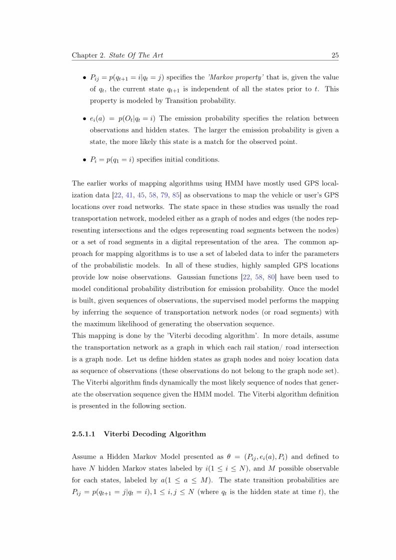
• Pij = p(qt+1 = i|qt = j) specifies the ’Markov property’ that is, given the value
of qt, the current state qt+1 is independent of all the states prior to t. This
property is modeled by Transition probability.
• ei(a) = p(Ot|qt = i) The emission probability specifies the relation between
observations and hidden states. The larger the emission probability is given a
state, the more likely this state is a match for the observed point.
• Pi = p(q1 = i) specifies initial conditions.
The earlier works of mapping algorithms using HMM have mostly used GPS local-
ization data [22, 41, 45, 58, 79, 85] as observations to map the vehicle or user’s GPS
locations over road networks. The state space in these studies was usually the road
transportation network, modeled either as a graph of nodes and edges (the nodes rep-
resenting intersections and the edges representing road segments between the nodes)
or a set of road segments in a digital representation of the area. The common ap-
proach for mapping algorithms is to use a set of labeled data to infer the parameters
of the probabilistic models. In all of these studies, highly sampled GPS locations
provide low noise observations. Gaussian functions [22, 58, 80] have been used to
model conditional probability distribution for emission probability. Once the model
is built, given sequences of observations, the supervised model performs the mapping
by inferring the sequence of transportation network nodes (or road segments) with
the maximum likelihood of generating the observation sequence.
This mapping is done by the ’Viterbi decoding algorithm’. In more details, assume
the transportation network as a graph in which each rail station/ road intersection
is a graph node. Let us define hidden states as graph nodes and noisy location data
as sequence of observations (these observations do not belong to the graph node set).
The Viterbi algorithm finds dynamically the most likely sequence of nodes that gener-
ate the observation sequence given the HMM model. The Viterbi algorithm definition
is presented in the following section.
2.5.1.1 Viterbi Decoding Algorithm
Assume a Hidden Markov Model presented as θ = (Pij , ei(a), Pi) and defined to
have N hidden Markov states labeled by i(1 ≤ i ≤ N), and M possible observable
for each states, labeled by a(1 ≤ a ≤ M). The state transition probabilities are
Pij = p(qt+1 = j|qt = i), 1 ≤ i, j ≤ N (where qt is the hidden state at time t), the

Chapter 2. State Of The Art 26
emission probability of observation at time t, Ot given state i is ei(Ot) = p(Ot|qt = i),
and the initial state probabilities are Pi = p(q1 = i).
Given a sequence of observations O = O1O2...OT , and an HMM θ = (Pij , ei(Ot), Pi),
Viterbi algorithm finds the maximum probability state path Q = q1q2...qT with a
dynamic programming approach.
Let vi(t) be the probability of the most probable path ending in state i at time t, and
generating the partial observation sequence O = O1O2...Ot,
vi(t) = maxq1,q2,...,qt−1
P (q1q2...qt−1, qt = i, O1O2...Ot|θ) (2.9)
and let wi be the initial probabilities of the states i at time t = 1.
Then vj(t) can be calculated recursively using:
vj(t) = ej(Ot)× max1≤i≤N
[vi(t− 1)× Pij ] (2.10)
together with initialization
vi(1) = Pi (2.11)
and termination
P ∗ = max1≤i≤N
[vi(T )] (2.12)
At the end we choose the highest probability endpoint, and then we backtrack from
there to find the highest probability path.
Note that the maximally likely path is not the only possible optimal criterion, for
example choosing the most likely state at any given time requires a different algorithm
and can give a slightly different result. But the overall most likely path provided by
the Viterbi algorithm provides an optimal state sequence for many purposes.
Fig. 2.2 illustrates how the Viterbi path is dynamically inferred.
The fundamental feature of mapping algorithms that have used HMM in previous
researches is that the underlying network is usually the road network. Other trans-
portation layers such as subway and train networks were not considered in such map-
ping algorithms. This is due to a couple of reasons: I) Collecting mobility data is
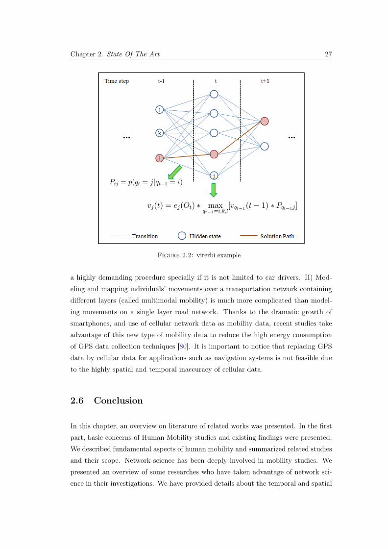
Chapter 2. State Of The Art 27
Figure 2.2: viterbi example
a highly demanding procedure specially if it is not limited to car drivers. II) Mod-
eling and mapping individuals’ movements over a transportation network containing
different layers (called multimodal mobility) is much more complicated than model-
ing movements on a single layer road network. Thanks to the dramatic growth of
smartphones, and use of cellular network data as mobility data, recent studies take
advantage of this new type of mobility data to reduce the high energy consumption
of GPS data collection techniques [80]. It is important to notice that replacing GPS
data by cellular data for applications such as navigation systems is not feasible due
to the highly spatial and temporal inaccuracy of cellular data.
2.6 Conclusion
In this chapter, an overview on literature of related works was presented. In the first
part, basic concerns of Human Mobility studies and existing findings were presented.
We described fundamental aspects of human mobility and summarized related studies
and their scope. Network science has been deeply involved in mobility studies. We
presented an overview of some researches who have taken advantage of network sci-
ence in their investigations. We have provided details about the temporal and spatial

Chapter 2. State Of The Art 28
scaleTransp
ortationLayer
Used
Model
Data
type
Related
Stu
dies
Regional
City
Road
Metro
Train
Air
EM
HM
MK
FC
DR
sG
PS
GSM
WiF
iH
uet
al.2003[41]
√√
√√
Hum
mel2006[44]
√√
√√
New
sonet
al.2009[58]√
√√
√
Thiagarajan
etal.2009[80]
√√
√√
√
Xu
etal.
2010[85]√
√√
√
Hunter
etal.
2011[45]√
√√
√
Thiagarajan
etal.2011[79]
√√
√√
Doyle
etal.2011
[30]√
√√
√
C.Y
.Goh
etal.2012
[22]√
√√
√
Smoreda
etal.2013[69]
√√
√√
√
Table
2.2:Sum
mary
Table
ofMapping
Algorithm
sm
entionedin
theliterature.
The
parameters
forthe
comparison
arescale
ofthestudy,
transportaionlayers,used
probabilisticm
odel(EM
:Expectation
Maxim
ization/
HM
M:H
iddenM
arkovM
odel/K
F:K
alman
Filter),and
differentdata
types.A
stable
shows,trajectory
mapping
inthe
citieshave
consideredonly
roadtransportation
layerand
haveused
mostly
GP
Sdata.

Chapter 2. State Of The Art 29
Scale Study Baseline Metrics Data type
Related Studies Cou
ntry
scal
e
Reg
iona
lsca
le
City
scal
e
Tra
ce-b
ased
stud
ies
Dyn
amic
prox
imity
netw
orks
Flo
won
netw
ork
Cen
tral
ity
mea
sure
Jum
ple
ngth
dist
ribu
tion
Rad
ius
ofgy
rati
on
GP
S
GSM
data
Wifi
Balcan et al.[10]√
Becker et al.[13]√
Yang et al. [84]√ √ √
Gonzalez et al.[16]√ √ √ √
Clauset et al. [18]√
Cs.Csajia et al. [21]√ √ √ √
Carske et al. [32]√ √
Giannotti et al.[34]√ √ √
Gonzalez et al.[36]√ √
P. Holme [38]√ √
Hunter et al.[45]√ √ √ √ √
Jiang et al.[47]√
Smoreda et al.[69]√ √ √
Thiagarajan et al. [79]√ √ √
Thiagarajan et al. [80]√ √ √
Wang et al.[83]√
Table 2.3: Summary table
issues of human mobility, opportunistic networks and centrality measures studied in
related fields.
To get a clear insight on specific features of mobility data, the second section was
dedicated to describe different types of mobility data in related studies. It was men-
tioned that mobility data plays the important role of setting spatial and temporal
constraints and scale for ongoing studies. We have seen that GPS data, despite its
fine spatial accuracy, suffers from high energy usage and thus is not practical for large
scale data collection due to the experiment cost. On the other hand, CDRs, in spite of
their great scalability to a large number of people and to large spatial scales, lack the
temporal granularity as they are sparse in time. We emphasized the importance of
mobility data in providing good enough granularity and scalability both spatially and
temporally. The third part of this chapter presents an outline of existing approaches

Chapter 2. State Of The Art 30
for trajectory mapping with an introduction to HMMs that forms the base of our
mapping algorithm. It was mentioned that using HMM in mapping noisy locations
of an individual trajectory over a transportation network was solely performed for
GPS data. A novelty of this work is dealing with the challenge of utilizing network
signalization data despite of their spatial inaccuracy for mapping over transportation
networks in urban and metropolitan areas in order to obtain an inference of individuals
real trajectory.

Chapter 3
Transportation Network Database
and Mobility Datasets
3.1 Introduction
After a literature review on the main aspects of human mobility and providing a
perception of the scope of the study and its challenges, this chapter provides an
outline of the network database and real trajectory datasets collected to model the
multimodal aspect of mobility in urban and metropolitan areas, which is the main
focus of this thesis. To do this, using different resources of open data, the multimodal
transportation network of Paris and its Region has been modeled and created, and
the resulting database has been employed in this work.
In addition, to conduct experiments, we have asked a group of volunteers with the
help of a french telecom operator, and we have collected their cellular trajectories
along with the associated detailed GPS trajectories.
Succinctly, three types of data are used in this study:
1. In order to construct the multimodal transportation network database that con-
tains all transportation modes (road/train/subway/tramway), geo-spatial data
have been collected from different open data sources.After collecting open data
from different sources, several data processing and transformation techniques
have been conducted to build the multimodal transportation network database.
31

Chapter 3. Multilayer Transportation Network and Multimodal Mobility Data 32
Figure 3.1: Three different data types that have been used in this PhD researchand their resources. 1.Geospatial data: open data from different sources (IGN/OS-M/RATP) collected to model and build the database. 2.Cellular signalization data
3.GPS data collected from participants cellphones using ’Moves’ application.
2. With the help of a french telecom operator, we have collected cellular signal-
ization data of a group of smartphone users. We recruited these users for one
month data collection experiment. The extracted real cellular trajectories were
used for testing the mapping algorithm.
3. For the sake of validation of the proposed algorithm , GPS data are used as
ground truth to assess the efficiency of the proposed mapping algorithm. The
GPS data were collected in a parallel data collection experiment for the same
group of users mentioned in the previous paragraph.
The variety of data resources that have been used to build the database and mobility
datasets are illustrated in figure 3.1 to clarify the distinctions. The following sections
describe the systematic procedures of data extraction, collection and processing to
obtain these datasets.

Chapter 3. Multilayer Transportation Network and Multimodal Mobility Data 33
Figure 3.2: In station ’Denfert Rochereau’ two metro lines and a train line meet
3.2 Multimodal Transportation Graph Databas
Currently, around 51% of the world population are living in cities and this percentage
is expected to reach 70% by 20501, accordingly urban mobility is one of the main
challenges in urban and metropolitan areas. Nowadays in cities and metropolitan
areas a variety of transportation modes cooperate in order to perform the population
mobility. Transportation modes such as subway, train, bike and bus are all cooper-
ating with each other to ensure efficient traffic in the cities and help individuals to
find a better and easier path to move from each origin to the preferred destinations.
Studies on smart cities have been trying to improve and optimize this cooperation
by detecting hubs and important locations as improving urban and transportation
system regarding the demand.
The word multimodal refers to having or involving several modes, modalities, or max-
ima 2 or having multiple or many modes or instances 3. Multimodal transport is the
articulation between different modes of transport, in order to transfer more rapidly
and effectively operations of materials and goods 4.
In the Human Mobility context, multimodal means having access to multiple modes
in daily commutes. In this dissertation, we use the term ’multimodal trajectories’
to describe trajectories that were generated through different transportation modes
(e.g. a trajectory that consists of a bus ride to a metro station and then a metro trip
to reach the destination). The concept of multimodal trajectories is familiar in peo-
ple’s daily life: Fig. 3.2 represents the rail public transportation map of Paris region1http://www.adlittle.com/downloads/tx_adlreports/ADL_Future_of_urban_mobility.pdf
2http://www.merriam-webster.com/dictionary/multimodal
3http://dictionary.reference.com/browse/multimodal
4http://www.slideshare.net/maxgalarza/multimodal-transport-3miridomemichellepedro

Chapter 3. Multilayer Transportation Network and Multimodal Mobility Data 34
Figure 3.3: The Multilayer transportation network is obtained by defining cross-layer links between different transportation layers
(Ile-de-France) that is available in all subway and train stations of the Ile-de-France
(Paris and its outskirts). Station ’Denfert Rochereau’ is an instance station where
two metro lines and one train line meet and people can change transportation modes
between subway and train and contrariwise.
Nevertheless, to meet the objective of this research work, we are required to have
a systematically designed multilayer transportation network in which different trans-
portation layers are considered and subsequently, ’mode changing’ between different
layers during a trajectory is feasible. We have modeled and built this network thanks
to an extensive data collection and data processing procedure. In the next sections,
we first present formal definitions of the multilayer transportation network and we
then describe data collection and database modeling and building.
3.2.1 Multimodal Transportation Graph Representation
Before addressing the technical aspects of multimodal transportation network con-
struction, this part describes the formal representation of the multimodal transporta-
tion network as a multilayer graph. The primary hypothesis is that each transporta-
tion layer is defined as a distinct layer. A proper description of the action of moving
from one layer to another is the key challenge in multimodal transportation network

Chapter 3. Multilayer Transportation Network and Multimodal Mobility Data 35
modeling and consequently in multimodal routing problems [54]. The multimodal
transportation network is represented according to the following definition:
Definition 1. Multilayer Transportation Graph
The Multilayer Transportation Graph is characterized as G = (V,E, L,Ψ) in which set
V represents the vertices of the graph, and Set E is the set of edges. Different possible
layers are distinguished by set L; in our study, we have: L = {road, train, subway}.Function Ψ is embedded in graph definition and indicates the layer of each node
Ψ : V → L in G.
Definition 2. Transportation Layer
The Transportation Layer is denoted as Gl = (V l, El), where each Gl is a subset of G.
V l is the node set of layer l and is represented as V l = {v|v ∈ V,Ψ(v) = l} . Likewise,
El is the edge set of layer l, where each edge connects two nodes both belonging to
layer l : El = {< vi, vj >∈ E,Ψ(vi) = Ψ(vj) = l}.Each node vi is characterized by its latitude and longitude (i.e., the geographical po-
sition vi =< lat, lon >i).
Definition 3. Cross-Layer Edge
The Multilayer Transportation Graph also contains Cross-Layer edges; set Ecl ⊂ E
includes the edges with pair of nodes not belonging to the same layer: Ecl = {<vi, vj >∈ G|Ψ(vi) = Ψ(vj)}. In other words, cross-layer edges enable the possibility
of defining a path whose nodes can belong to different transportation layers.
The multilayer Transportation graph is represented by its adjacency matrix Wij ∈R|V |×|V |. Fig. 3.3 illustrates how cross-layer links are added to different transporta-
tion layers to build a multimodal transportation network.
In the next section the procedure of data extraction for network construction is ex-
plained.
3.2.2 Data Extraction for Network Construction
To build the multilayer transportation graph G, multiple geospatial datasets, namely
the road network from the National Geographic Institute (IGN)[1] and the rail trans-
port network (train and metro) from OpenStreetMap (OSM)[3] were aggregated. Each
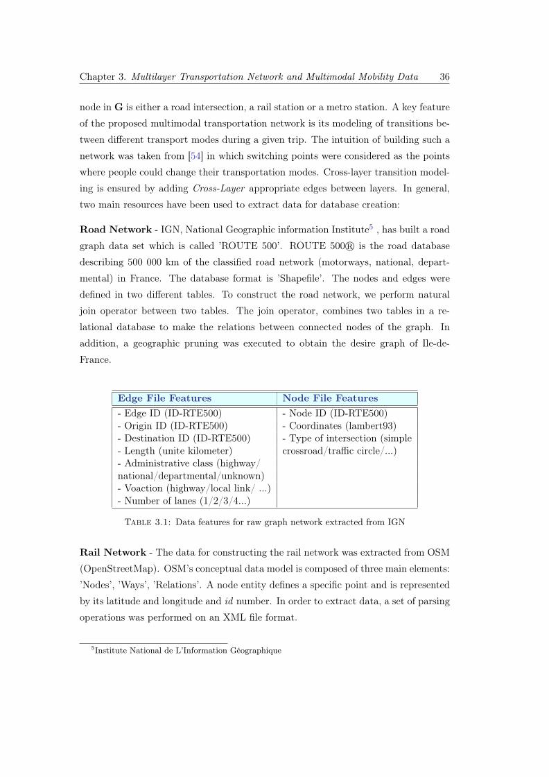
Chapter 3. Multilayer Transportation Network and Multimodal Mobility Data 36
node in G is either a road intersection, a rail station or a metro station. A key feature
of the proposed multimodal transportation network is its modeling of transitions be-
tween different transport modes during a given trip. The intuition of building such a
network was taken from [54] in which switching points were considered as the points
where people could change their transportation modes. Cross-layer transition model-
ing is ensured by adding Cross-Layer appropriate edges between layers. In general,
two main resources have been used to extract data for database creation:
Road Network - IGN, National Geographic information Institute5 , has built a road
graph data set which is called ’ROUTE 500’. ROUTE 500® is the road database
describing 500 000 km of the classified road network (motorways, national, depart-
mental) in France. The database format is ’Shapefile’. The nodes and edges were
defined in two different tables. To construct the road network, we perform natural
join operator between two tables. The join operator, combines two tables in a re-
lational database to make the relations between connected nodes of the graph. In
addition, a geographic pruning was executed to obtain the desire graph of Ile-de-
France.
Edge File Features Node File Features- Edge ID (ID-RTE500) - Node ID (ID-RTE500)- Origin ID (ID-RTE500) - Coordinates (lambert93)- Destination ID (ID-RTE500) - Type of intersection (simple- Length (unite kilometer) crossroad/traffic circle/...)- Administrative class (highway/national/departmental/unknown)- Voaction (highway/local link/ ...)- Number of lanes (1/2/3/4...)
Table 3.1: Data features for raw graph network extracted from IGN
Rail Network - The data for constructing the rail network was extracted from OSM
(OpenStreetMap). OSM’s conceptual data model is composed of three main elements:
’Nodes’, ’Ways’, ’Relations’. A node entity defines a specific point and is represented
by its latitude and longitude and id number. In order to extract data, a set of parsing
operations was performed on an XML file format.
5Institute National de L’Information Géographique

Chapter 3. Multilayer Transportation Network and Multimodal Mobility Data 37
Edge Entity Features Node Entity Features- Edge ID (OSM-id) - Node ID (OSM-id)- Origin ID (OSM-id) - Coordinates (WGS84)- Destination ID (OSM-id)- Network type (subway,train, tramway, RER)
Table 3.2: Data features for rail network extracted from OSM
3.2.3 Multimodal Transportation Network Database
3.2.3.1 Data Model
The conventional data model to represent transportation networks is a graph data
model. In this work, we use a graph data model to define the transportation network
as the set of nodes and edges that were formally presented in section 3.2.1.
3.2.3.2 Database Model
After defining the data model, the next step is to define a database model which
specifies the logical structure of a database and fundamentally determines in which
manner data can be stored, organized, and manipulated. It is important to notice that
in our work, the data model is a ’graph model’, but the database model is a’document
model’. In this work, we use MongoDB a document database system to implement
the transportation network database. Every data element in MongoDB is stored in
a JSON-style object called a document. An advantage of MongoDB is its flexible
data structure: everything is stored as a document, which allows us to add or remove
properties. A graph containing nodes and edges can fit properly in this structure.
In addition, MongoDB offers a number of indexes and query mechanisms to handle
geospatial information by supporting GeoJSON object types. GeoJSON is an open-
source specification for the JSON-formatting of shapes in a coordinate space. It is a
format for encoding a variety of geographic data structures. A location data point can
be stored as GeoJSON object with this coordinate-axis order: longitude, latitude. The
coordinate reference system for GeoJSON uses the WGS84 datum. Each GeoJSON
document (or subdocument) is generally composed of two fields:
1. Type the shape being represented, which informs a GeoJSON reader how to
interpret the "coordinates" field.

Chapter 3. Multilayer Transportation Network and Multimodal Mobility Data 38
Figure 3.4: Left: A graph node stored as a ’Point’ geometry object; right: a graphedge stored as a ’LineString’ geometry object in the document database
2. Coordinates an array of points, the specific arrangement of which is deter-
mined by "type" field.
A geometry is a GeoJSON object where the type member’s value is one of the following
strings: "Point", "MultiPoint", "LineString", "MultiLineString", "Polygon", "Multi-
Polygon", or "GeometryCollection". Accordingly, all these objects are supported by
MongoDB. A GeoJSON geometry object of any type other than "GeometryCollec-
tion" must have a member with the name "coordinates". The value of the coordinates
member is always an array. The structure for the elements in this array is determined
by the type of geometry. Consequently the simplest geometry can be represented as:
{
"type": "Point",
"coordinates": [long, lat]
}
To implement the graph data model using GeoJSON format, each node is represented
as a "Point" object type and each edge as "LineString". A set of common keys to
store the properties of nodes and edges have been characterized. Fig. 3.4 presents two
documents that describe node and edge of the graph. Subsequently, the CrossLayer
edges are defined to make connections between each two nodes belonging to different
transportation layers that are close enough to each other. We used a radius of 500
meters as the threshold of the closeness definition. In another similar work [71], for

Chapter 3. Multilayer Transportation Network and Multimodal Mobility Data 39
(a) Road (b) Train
(c) Subway (d) Multilayer
Figure 3.5: Different transportation layers and their expansion in Paris region
the simplification of the problem, each subway station is connected to its closest road
intersection.
All the process of data integration (data cleaning, geographical pruning , etc.) were
implemented using Python script, while graph formation and graph analysis were
done by the help of the ’NetworkX’ library.
3.2.4 Graph Statistics
This section is dedicated to inspection and examination of the multiomodal trans-
portation network. The objective is to investigate the features and behavior of the
multimodal graph G. We present a statistical analysis of multimodal transportation
network to illustrate the fundamental properties of each transportation layer.
Although such a multilayer representation of the transportation network enables us to
model and define trajectories using different transportation modes, it also increases the

Chapter 3. Multilayer Transportation Network and Multimodal Mobility Data 40
complexity of the underlying network. Table 3.3 summarizes the topological features
of different transportation layers. It clearly illustrates topological differences between
each layer in the multilayer graph G. For example, the average length between two
consecutive intersections is rather heterogeneous across different transportation lay-
ers. This heterogeneity is observed for other features as well.
The area of study is this research work, Ile-de-France (also known as "Paris Region")
with the area of 12, 012 km2, has a typical radiocentric urban structure that benefits
from different public transportation networks. It is important to notice that coverage
area of these transportation systems are dissimilar as is illustrated in Fig. 3.5. The
subway layer illustrated in Fig. 3.5c covers fairly the central part of Paris region with
the area of 105 km2 and some part of inner ring with the coverage area of 657 km2.
The train layer is well expanded in the inner ring area and provides some coverage in
the southern part of the outer ring area with 11, 250 km2 coverage (Fig. 3.5b). There
are areas which are not covered neither by rail transportation layer nor by subway
transportation layer; these areas are visible in Fig. 3.5d.
Table 3.3 presents basic features of different transportation networks. As the table
illustrates, the multilayer graph is essentially dominated by the road network.
Layer name |N | |E| < k > < l > (km) Diamtopo < SP > Reference
Subway 303 356 2.35 0.757 34 12.21 OSMTrain 299 303 2.027 3.07 47 16.54 OSMRoad 14798 22276 3.01 1.34 135 51.1 IGNMultimodal 15342 26947 3.51 0.87 114 36.51
Table 3.3: Different transportation layers and their main features: number ofnodes |N |and edges |E|, average node degree < k >, average edge length < l >,diameter and average shortest path < sp > and their data references are indicated
3.3 Multimodal Cellular Trajectories Dataset
This section describes the cellular trajectory used in this study. For obtaining the
trajectory dataset, we applied a new approach to collect cellular signalization data
of smartphone users. As described in chapter 2, despite the spatial inaccuracy of
cellular data, this method insures a constant sampling rate that enables us to obtain
uniformly sampled cellular locations. Such a property cannot be insured with CDRs.
This improvement in the temporal dimension enables us to extract sparse cellular tra-
jectories of users that are more adequate for mapping than CDR trajectories. Fig. 3.6

Chapter 3. Multilayer Transportation Network and Multimodal Mobility Data 41
is an example of cellular trajectories of a user collected during 100 days. As the figure
shows, the cellular signalization data are capable to reflect the mobility of individuals.
Table 3.4 illustrates four rows of the data table collected by this method. The raw
data table contains userID, unix timestamp of the messaging time, the milliseconds
of the time stamp (ms), type of "tunneling management message" (Msg type) and
the geospatial coordinate of the antenna as ’latitude’ and ’longitude’.
UserID UNIX TIMESTAMP ms Msg Type Latitude Longitude110003934 1363419350 63957 17 48.864901 2.409734110003934 1363419401 697412 18 48.864929 2.409725110003934 1363419401 495528 19 48.864967 2.409754110003934 1363419744 497542 20 48.864054 2.409702
Table 3.4: subsample of raw cellular signalization data
The Cellular trajectory dataset that have been used in this work, has been collected
from a group of smartphone users with the help of a french telecom company. The
frequency of data sampling is 15 minutes and consequently, the extracted trajectories
are called sparse cellular trajectories. To extract the cellular trajectories of users from
given raw data, a set of data preprocessing techniques have been performed.
Figure 3.6: Cellular signalization data of a smartphone user during 100 days in Parisand vicinity. Blue circles are the most frequent visited places
First, we set a ’waiting time cutoff’ as the maximum allowed time between two con-
secutive cell records in the same trajectory. A trajectory is started from the first
movement (a change in cell position) and it ends when the difference between two

Chapter 3. Multilayer Transportation Network and Multimodal Mobility Data 42
consecutive time stamps are more than value ∆c where ∆c (we set ∆c=30 min). Each
trajectory is a sequence of time stamped locations such as the time stamp difference
for each two consecutive distinct locations is not bigger than ∆c. This restriction
means that if a user stays at the same location for more than ∆c, the trajectory
ends in that location. In this step, each trajectory is a sequence of time-stamped cell
locations. However, not all the sequences are suitable for trajectory mapping. The
radius of gyration defined in equation 2.3 is used to filter out the trajectories whose
radius of gyration is smaller than a selected threshold Drg . Fig. 3.7 illustrates two
trajectories with different scales of gyration radius. Given the spatial inaccuracy and
the temporal sparsity of cellular data, we are interested in trajectories whose gyration
radius is higher than a threshold Drg (e.g. 2 KM).
Figure 3.7: Two cellular trajectories with different radius of gyrations.
Definition. Cellular Trajectory
A cellular trajectory of a user is presented as a sequence of time-stamped locations
O = o0 → o1... → oM , where each time-stamped location ot =< c(t) > refers to the
cell tower at time-stamp t the user is observed at.
3.4 Multimodal GPS Trajectories Dataset
This section presents an overview of the multimodal GPS trajectory dataset con-
taining records of multimodal trajectories. A multimodal trajectory is defined as a
trajectory involving several modes of transportation. The majority of mobility studies
using GPS trajectories, have considered monomodal trajectories (e.g involving only
the road transportation network) while in multimodal mobility studies, it is crucial to
consider trajectories taking place using different transportation modes. To the best of
our knowledge, there exists no real GPS dataset that covers individuals’ trajectories
over a multimodal transportation network. In this research study, to evaluate and

Chapter 3. Multilayer Transportation Network and Multimodal Mobility Data 43
validate our proposed algorithms, we conducted a data collection experiment to col-
lect fine-grained multimodal trajectory data that will serve as ground truth for sparse
cellular trajectories.
Figure 3.8: An example of multimodal trajectory, presented in different colors:red lines are the paths that the individual takes to walk to or from a metro station
while the blue line is the trip path which is carried out by metro.
To collect the ground truth data, the recruited group were asked to install application
’Moves’ [2]. The data captured by the application is classified in different categories
’Walking’, ’Running’, ’Cycling’ and ’Transport’. With a series of interviews, the trans-
portation mode of trajectories have been specified. Fig. 3.8 illustrates an example of
multimodal trajectory in which an individual walks to the metro station (red line) and
then walks from metro station to the final destination. As illustrated in the figure, a
multimodal trajectory may consist of different sub-trajectories, each taking place on
one specific transportation layer. By modeling and building the multimodal trans-
portation network, it is possible to represent a multimodal trajectory as a sequence
of nodes over the multimodal graph; such a case of study was not addressed before.
The collection of the GPS trajectories dataset was performed simultaneously with Cel-
lular data collection for the same group of volunteers over the period of the sampling
(Aug-Sept. 2014). The dataset covers 130 hours of walking and 470 hours of trans-
portation which is not limited to road and contains multimodal trajectories. Figure
3.9 shows the coverage area of collected the GPS trajectory dataset. The trajectories
are mapped over the multimodal transportation network containing road, train and
metro layers. It is also important to notice that for underground trajectories there
were missing data which were corrected manually after interviews with volunteers.

Chapter 3. Multilayer Transportation Network and Multimodal Mobility Data 44
Figure 3.9: The coverage area of GPS data collected is shown in yellow on themap of Paris and region
0 10 20 30 40 50 60 70 80Trajectory length (KM)
0.00
0.01
0.02
0.03
0.04
0.05
0.06
Pro
bab
ilit
y
∆t=5 min
∆t=10 min
∆t=20 min
∆t=30 min
Trajectories Length Distribution
(a) Length distribution
0 50 100 150 200Trajectory time (Minutes)
0.000
0.005
0.010
0.015
0.020
Pro
bab
ilit
y
∆t=5 min
∆t=10 min
∆t=20 min
∆t=30 min
Trajectories Time Distribution
(b) Time distribution
Figure 3.10: Distribution of trajectory lenth and trajectory time for a range of∆t waiting time cutoff are plitted
It is worth to mention that for GPS trajectory extraction, a ’waiting time cutoff’ was
used to separate different movement activities and to make distinction between them.
Figure 3.10 presents some statistics on the multimodal trajectory dataset extracted
from GPS collected data.
3.5 Conclusion
This chapter provided an overview of database modeling and building of cellular and
GPS trajectories’ extractions. The first part covered the steps carried out to build a

Chapter 3. Multilayer Transportation Network and Multimodal Mobility Data 45
multilayer graph database. We described how the data model of the multimodal trans-
portation network was defined as a graph of nodes and edges and how its database
was implemented using a document oriented database system. The advantages of
a document database system and specifically MongoDB is that it provides an effi-
cient standard for storing and querying geospatial objects. Such a system is a proper
choice for storing a multimodal graph in which nodes and edges have different prop-
erties but are all considered as geometry objects. The constructed database is related
to Ile-de-France which is used in next chapters as the study area. The mutlimodal
transportation networks of other areas could be constructed in the same way. The
main advantage of the modeled transportation network is that it sets no constraint in
multimodal trajectory representation. Accordingly, a multimodal trajectory involving
different transportation layers is defined as a path over the multilayer transportation
network. The nodes of the graph could belong to different transportation layers and
the action of mode changing is duly represented as cross-layer edges.
In the second part of this chapter, the cellular signalization dataset and its character-
istics are described. This section outlined the procedure to extract the users sparse
cellular trajectories as sequences of time-stamped antenna locations.
Ultimately, the last part of this chapter introduced the multimodal GPS trajectory
database and its features. The trajectories in this dataset can be defined as sequences
of nodes where nodes are either road intersections or subway/train stations. That is,
the multimodal transportation network database provides a geospatial reference that
will be used in the rest of this work to represent the trajectories of individuals.
The multimodal transportation network and cellular trajectory dataset will be used in
the following chapters to develop the mapping algorithm. For qualitative assessment,
the GPS trajectory dataset will serve as labeled data to evaluate the accuracy of our
proposed algorithms.


Chapter 4
Methodology:CT-Mapper
Mapping Sparse Cellular
Trajectories to Multimodal
Transportation Network
4.1 Introduction
Macroscopic analysis of the traffic flow in large metropolitan areas is a challenging
task. This is especially true when multiple transit authorities are in charge of different
transport networks (road, train, subway). Due to the lack of a common source of
information across these transit systems, it is often hard for city authorities to grasp
a unified view of mobility patterns. In this context, mobile phone data have recently
become an attractive source of information about mobility behavior. Thanks to the
ubiquitous usage of mobile phones, mining mobile phone data becomes a promising
way to understand multimodal human mobility [30, 63, 69] ranging from identifying
a mobile user daily path to recording transportation usage (e.g., taking train, metro,
bus, etc.) in a large metropolitan area. Traditional approaches of mobility studies
used GPS to accurately sense spatial data with a localization error bound ≤ 50m.
Although they ensure the collection of fine-grained mobility trajectories (as shown in
Fig. 4.1b), GPS-based data collection has two main drawbacks: first, it causes high
energy consumption, and second, it is constrained to a limited group of users (e.g. taxi
47

Chapter 4. Methodology : CT-mapper 48
drivers [50] or a group of car drivers [34]). GPS sensing, therefore, is not suitable for
collecting large-scale data from metropolitan area populations. By contrast, cellular
data provided by network operators does not suffer from these issues, and has become
recently, as a result, a new source of mobility information. Signaling information from
mobile network operators (CDRs -Call Data Records-) has been used as a valuable
source of mobility information for large scale population [4, 24, 69].
Localization of mobile phone users with antennas (i.e., cellular towers), nonetheless,
provides only coarse-grained mobility trajectories at antenna level, with a varying
localization error of hundred meters in densely populated cities, and within several
kilometers in rural areas [69]. Given the resulting cellular mobility trajectories (i.e.,
a sequence of antenna ids) and the location of each antenna as shown in Figure 4.1c,
it might be difficult to observe the road or metro station that the user passes by (as
shown in Fig. 4.1a).
In order to collect cellular mobility trajectories using mobile phones, previous works [4,
24, 69] usually extracted the trajectories from Call Detailed Records (CDR), where
the CDR of a user restores the antenna id and the time-stamp of each of his/her
mobile calls. To understand human mobility, these works were mostly limited to ag-
gregating the trajectories from a user’s long-term CDR data in order to determine the
frequently-visiting locations and the visiting time (e.g., the park he/she usually passes
by during the 07:00–09:00 window of working days). As such, the techniques proposed
by previous works are not suitable for estimating the precise mobility trajectories on
the road/transportation network using the CDR cellular trajectories. Furthermore,
one sample of CDR data (i.e., one call record) can be obtained only when the user
places a call, making human mobility data between two consecutive calls irretrievable,
especially when the time duration between the two calls is long (e.g., the inter-call
mobility between the two calls in Fig. 4.1d). Thus, even though it has been studied
widely, CDR is unlikely to be a good data source for the trajectory mapping problem.
Considering the time sparsity drawbacks of CDRs, we use, in this work, a new passive
capturing technique to efficiently extract the position of the base stations the mobile
phone connects to. This technique analyzes the signaling channel of the data mobile
network in order to extract base station locations. This way of capturing the mobility
of users is scalable and provides a higher sampling rate than CDR-based sensing.
The sparse cellular trajectories are collected and provided upon the request of the
experiment participants to the network operator. Considering privacy issues [51], the
network operator localizes each mobile user using an antenna id, and further records

Chapter 4. Methodology : CT-mapper 49
(a) Road Trajectory (b) GPS Trajectory
(c) Cell Trajectory (Full) (d) CDR Trajectory
(e) Sparse Cell Trajectory
Figure 4.1: A user’s trip from Airport CDG to city center of Paris: The roadtrajectory consists of the sequence of roads that the user passes-by; The GPS tra-jectory is sampled in minute based frequency; The Cellular trajectory (Full) recordseach cell tower the user passes-by; The CDR trajectory reports the location of theuser’s each call during the trip; The Sparse Cellular trajectory is sampled every 15
minutes

Chapter 4. Methodology : CT-mapper 50
each user’s antenna id with time-stamp periodically (e.g., every 15 minutes in our
study). Compared to the user’s real trip (in Fig. 4.1a), the sparse cellular trajectory
(in Fig. 4.1e) partially measures the user’s mobility with coarse-grained localization.
The objective of our work is to map each sparse cellular trajectory into the multimodal
transportation network, in order to obtain the sequence of network nodes that the
user passes by. For example, given the cellular trajectory shown in Fig. 4.1e and the
transportation network of the Paris metropolitan area shown in Fig. 4.2, our goal is
to recover the sequence of nodes of the real trip shown in Fig 4.1a.
The common approach for mapping cellular trajectories into the metropolitan trans-
portation (usually road in the state of the art) network is to first collect a large amount
of cellular trajectories and then to manually label each with the corresponding inter-
section sequence, an intersection being a graph node associated with a junction be-
tween two roads. The next phase is to train a supervised mobility model (e.g., HMM)
using the labeled cellular trajectories, in order to build a probabilistic model mapping
antenna id sequences to intersection sequences. After training, given a new user cel-
lular trajectory, the supervised model predicts, as the mapping result, a sequence of
intersections, having the maximal likelihood of generating the antenna id sequence.
However, obtaining the labeled cellular trajectories to cover the road/transportation
networks and all cellular towers of a metropolitan area is not practical, as it costs
too much human efforts for trajectory collection and labeling. We propose, in this
chapter, to solve the cellular trajectory mapping problem using an unsupervised
model, that does not require collecting and labeling any trajectories.
Given the above examples and target research goals, the key issues in designing the
unsupervised mobility model include:
1) Given the antenna id sequence in a cellular trajectory, retrieve the sequence of road-
/rail intersections that the user passes by given a database storing the multimodal
transportation network - The transportation network covering and connecting
multiple types of transportation modes (e.g., rail, metro, highway , etc.) is named
multimodal transportation network [54], in which each node is either a road inter-
section or a station of a rail transportation mode (i.e., subway, tramway and train),
and each edge is a connection between intersections (e.g., the pathway connecting a
metro station and a bus stop). Obviously, it is nontrivial to extract the precise user
path from the multimodal transportation network using the antenna id sequences.
The cellular trajectory might come from multiple transportation systems nearby each
corresponding antenna and in different layers (underground, ground and trestle). To

Chapter 4. Methodology : CT-mapper 51
overcome this issue, it is necessary to build a comprehensive database storing all the
intersections of the multimodal transportation network, where we can accurately re-
trieve the surrounding intersections of each antenna. In this work, open data provided
by OpenStreetMap (OSM) and the National Geographic Institute (IGN) are used to
extract the multimodal transportation network of Ile-de-France (Paris and vicinity).
This region is characterized by a high diversity of public transportation modes (sub-
way, tramway, RER, train, bus) that have each particular specifications. Therefore,
building a multimodal transportation network to study individuals’ mobility requires
a clear understanding of the multimodal network complexity. The multimodal trans-
portation network is modeled in this work based on the concept of ’cross-layer’ links
that connect each two nodes where users can switch transportation modes.
2) Given an observed cellular trajectory, compute the most-likely intersection se-
quence over the multimodal transportation network - It is difficult to search the
most-likely intersection sequence from the set of intersections, due to the following
reason:
Likelihood Computation: In order to search the most-likely intersection sequence,
given an observation sequence, we need to calculate the likelihood of each node given
the cellular trajectory. While the traditional supervised HMM mobility model har-
nessing the statistics of labeled cellular trajectories (i.e. emission/transition proba-
bilities) is usually used to estimate the likelihood, we propose an unsupervised HMM
that does not leverage labeled data. Rather it proposes a method to calculate the
likelihood using the topological properties and other information of the transporta-
tion network. In other words, the HMM parameters are automatically derived in an
unsupervised way based on a priori knowledge of transportation network properties.
In summary, the main contributions of this work are:
• We propose to study the problem of mapping cellular trajectories to the mul-
timodal transportation network, in order to obtain the precise mobility of the
users. To the best of our knowledge, this is the first work addressing these
issues. In particular, rather than mapping cellular trajectories using the su-
pervised mapping algorithms with labeled mobility data, we propose to use
an unsupervised mapping algorithm leveraging on topological properties of the
transportation network, so as to eliminate the tedious human labeling efforts in
building the mobility model.

Chapter 4. Methodology : CT-mapper 52
• We propose an unsupervised trajectory mapping algorithm, namely CT-Mapper,
which maps cellular location data over the multimodal transportation network.
The multimodal transportation network database was built using different ref-
erences of geospatial resources. The mapping algorithm is modeled by an HMM
where the observations correspond to user cellular trajectories and the hid-
den states are associated with nodes of the multilayer graph which are either
road intersections or subway/train stations. Transition probability and emis-
sion score were modeled based on topological properties of the transportation
network and the spatial distribution of antenna base stations. Viterbi decoding
algorithm helps reduce the complexity of finding the best match which might
enable us to deploy our unsupervised mapping algorithm on large scale mobility
data sets in order to estimate multimodal traffic in metropolitan areas.
The rest of this chapter is structured as follows: section 4.2 presents related work.
Section 4.3 gives an overview of the proposed system. Section 4.4 presents the details
of the unsupervised estimation of HMM parameters and explains how the two main
probability distributions used for mapping are derived and the chapter ends by a
discussion and a conclusion in section 4.5.
4.2 Related Work
4.2.1 General Human Mobility Models
A considerable amount of Human Mobility studies have been devoted to analyze tra-
jectories of individuals based on their traces. Spatial characteristics such as center
of the mass, radius of gyration and statistical characteristics revealed a number of
scaling properties in human trajectories: Gonzalez et al in [16] and Brockmann et al
[15] showed a truncated power-law tendency in the distribution of jump length. It
was observed that most individuals travel only over a short distance, and there is only
a few who travel regularly over hundred kilometers. Further studies [36] [16] showed
that travel patterns collapse into a single spatial probability distribution, indicating
that, despite the diversity of their travel history, humans follow simple reproducible
patterns. In addition, statistical analysis confirms that individuals’ movement follows
spatio-temporal patterns [34] [33] [21] which can help defining mobility models. In
all mentioned studies, multimodal mobility aspects were not taken into account. One
objective, in this work, is to investigate the mobility patterns of trajectories through

Chapter 4. Methodology : CT-mapper 53
the multimodal transportation network and to explore how these patterns are affected
by the multiplicity of the layers of the network. Early mobility studies relied on ex-
pensive data collection methods, such as surveys and direct observation. Trajectories
were mostly defined as Origin-Destination (OD), and were mapped over the desirable
graph to retrieve an optimal path solution which is usually the shortest path between
the Origin and Destination [33, 34, 36, 87]. Although recent studies have been trying
to infer the traffic flow using additional traffic data [5], they still fail to retrieve the
real path taken by individuals.
4.2.2 Mapping Algorithms
Along with mobility studies, applications such as navigation systems, traffic mon-
itoring and public transportation tracking, used GPS data to track individuals or
any moving object [22, 41, 45, 58, 79, 85]. A variety of statistical approaches such
as Expectation Maximization (EM) [45], Kalman Filter [41, 85] and Hidden Markov
Model (HMM) [22, 44, 58, 79, 80] were used to map ’noisy’ sequential location data
over transportation networks. Most of these mapping algorithms have used GPS data
as they provide accurate location data with an error of about 50 meters. Moreover,
using labeled data, supervised models were considered and trained to optimize model
parameters in an automatic way. Once the models are trained, they are used to find
the most likely path in the network assigned to sequences of ’noisy’ location data.
However, most of these mapping algorithms were developed to map noisy data over
road networks without considering other mobility modes.
4.2.3 Human Mobility Modeling with CDR Cellular Trajectories
Recently, because of the expeditious growth of mobile phones, Call Data Records
(CDR) have been providing great data sets for human mobility studies as they are
collected continuously for all active cellular phones. CDRs, however, have two sig-
nificant limitations: first, they are sparse in time because they are generated only
when a phone engages in a voice call or text message exchange; and second, they are
coarse in space and less precise than GPS location data, because they record location
only at the granularity of a cellular antenna (with an average error of 175 meter in
dense populated areas and up to 2 kilometers in less denser areas). Nonetheless, the
fact that almost the entire population is already equipped with cell phones [69] allows
for studying important aspects of individual mobility such as inferring transportation

Chapter 4. Methodology : CT-mapper 54
modes. Cellular network data were, for instance, used to classify different transporta-
tion modes for long-distance travels [30, 69]. Thiagaran et al. in [79] used cellular
signal data with combination of cellphone sensors to develop a supervised mapping
algorithm in order to overcome the limitation of GPS data. While previous works
have used cellular data to map long trajectories, this work proposes an unsupervised
mapping algorithm that maps the sparse cellular trajectories over the multimodal
transportation network in the Paris metropolitan area. This approach could be used
for large scale smart-phone users for further studies in traffic estimation. Such a
mapping is important for the development of smart cities and smart mobility. Stud-
ies of smart cities in the past were limited to analyzing multimodal transportation
networks without considering large scale real mobility data. The main goal of multi-
modal mobility studies is to improve public transportation monitoring and to reduce
traffic congestion [7, 54, 56] . Considering the aforementioned observations and the
fact that the majority of trajectory mapping problems are developed for mono-modal
transportation networks (specifically road networks), we believe that there is a gap
in the literature. This study aims at bridging this gap by mapping cellular sparse
data of smartphones over the multimodal transportation network in the Ile-de-France
metropolitan area. The multimodal mapping results may help not only optimizing the
multimodal transportation network, but also investigating the multimodal mobility
behavior of individuals in metropolitan areas.
4.3 CT-Mapper System Overview
In this section, we first formulate the search problem of CT-Mapper, and introduce
the datasets collected for mapping. We then analyze the computational complexity of
the mapping problem over the collected datasets, and finally present the framework
of CT-Mapper.
4.3.1 Problem Statement
In this section, we first formulate the problem be defining several key concepts used
in our approach.
Definition 1. Multilayer Transportation Graph - Such a graph is represented
as G = (V,E,L,Ψ) where V , E represent the vertices and the edges, L is the set of
possible layers. In our study we focused on 3 layers: road, train and subway.

Chapter 4. Methodology : CT-mapper 55
Figure 4.2: Multilayer representation of different transportation networks
Function Ψ indicates the layer of each node Ψ : V → L in G.
Transportation Layer Gl = (V l, El) is a subset of G, where V l = {v|v ∈ V,Ψ(v) = l}and El = {< vi, vj >∈ E,Ψ(vi) = Ψ(vj) = l}. Each node vi is characterized by its
latitude and longitude (i.e., the geographical position vi =< lat, lon >i)
CrossLayer edge set Ecl ⊂ E defines the edges with pairs of nodes not belonging to
the same layer: Ecl = {< vi, vj >∈ G|Ψ(vi) = Ψ(vj)}The multilayer Transportation graph is characterized by its adjacency matrix Wij ∈R|V |×|V |. Fig. 4.2 illustrates how different transportation layers have been aggregated
to build a multimodal transportation network.
Definition 2. Cellular Network - In this work, we characterize a cellular network
as a set of cell towers C = {c0, c1, ...cP }, where each cell tower cp =< lat, lon, rmax >p
is characterized by its latitude and longitude in the geographical coordinate system
and by rmax which is the maximum radius of the voronoi cell the cell belongs to in
the voronoi graph built from set C. Please note that the location of each cell tower
does not coincide with the location of any intersection in the transportation network
i.e., ∀vi ∈ V , ∀cp ∈ C, we have < lat, lon >p = < lat, lon >i.
Definition 3. Sparse Cellular Trajectory - Further we define a sparse cellular
trajectory of a user as a sequence of time-stamped locations O = o0 → o1... → oM ,
where each time-stamped location ot =< c(t) > refers to the cell tower at time-stamp
t the user is observed at.

Chapter 4. Methodology : CT-mapper 56
Figure 4.3: Voronoi tessellation of cellular antennas in Ile-de-France
Trajectory Mapping Problem - Given a transportation network G, cell tower
network C, and a user sparse cellular trajectory O, our search problem is to find a
sequence of intersections v0 → v1... → vq which the user actually passes by on the
transportation network.
4.3.2 Data Collection and Datasets
Three types of data are used in this study: multimodal transportation network data,
sparse cellular trajectory data, and GPS trajectory data. The multimodal transporta-
tion network data are used to build the multilayer network graph and the mobility
model for the mapping algorithms. Cellular trajectories are used for testing while
GPS trajectories are used as ground truth and not for training HMM parameters.
Sparse Cellular Trajectory Data - In this work we use a new type of cellular tra-
jectory named Sparse Cellular Trajectory. A set of techniques for data collection are
used to capture GPRS Tunneling Protocol (GTP) messages from the Cellular Data
Network. Packet inspection of GTP-C (GTP control plane) enables us to capture
users’ localization information at higher frequency than the usual CDR. The GTP is
the tunneling protocol used to carry data traffic over the mobile network (from 2G
to LTE) to internet. When a smartphone enables its internet connection (e.g. when
it is turned on), a message is sent over the network asking for access. This message
contains among other things the identity of the phone and the cell id covering the
user. Once the session is established, update messages are sent carrying information

Chapter 4. Methodology : CT-mapper 57
like the bearer or the cell id. These messages are triggered when the user moves from
a BTS to another or by resource allocation. Finally, when the mobile looses the signal
or is turned off, a message closing the session is sent. With modern smartphone ap-
plications that emit and receive data on a regular basis (i.e. email, push notification),
it is expected that the GTP tunnel for a given user remains constantly maintained,
enabling us to sample the user position at each network event (handover and radio
resource allocation).
GPS Trajectory Data - To evaluate the accuracy of our proposed mapping algo-
rithm, GPS data were used as ground truth. A group of participants were asked to
install the "Moves" smartphone application [2] to record their GPS locations. The
GPS locations provided by "Moves" were analyzed to extract real trajectories of par-
ticipants.
4.3.3 Computational Complexity of the Mapping Problem in theCollected Datasets
Layer name |N | |E| < k > < l > (KM) Reference
Subway 303 356 2.35 0.757 OSMTrain 241 244 2.025 3.07 OSMRoad 14798 22276 3.01 1.34 IGN
Table 4.1: Different transportation networks with four main features: number ofnodes (|N |), number of edges (|E|), average degree (< k >) and average edge length
(< l >)
The underlying transportation network used in this study is the multimodal trans-
portation network of Ile-de-France which is modeled by several separated graph layers
corresponding each to a different transportation mode, interconnected together into
a multilayer graph G. To build this graph, multiple geospatial datasets, namely the
road network from the National Geographic Institute (IGN)[1] and the rail transport
network (train and metro) from OpenStreetMap (OSM)[3] were aggregated. Each
node in G is either a road intersection, a rail station or a metro station. A key
feature of the proposed multimodal transportation network is its modeling of tran-
sitions between different transport modes during a given trip. Cross-layer transition
modeling are ensured by adding CrossLayer appropriate edges between layers.
To quantitatively assess network complexity, we use entropy measure to characterize
the ease/difficulty of navigation in a network using "the search information" developed

Chapter 4. Methodology : CT-mapper 58
in [70], and in [65].
Eq. (4.1) defines the probability for a random walker starting at node s with degree
ks to reach node t through the shortest path SPst. Consequently, in eq. (4.2) we
define the search entropy of a graph as the sum over all shortest paths {SPst} from
node s to node t in G averaged over all possible pair of nodes (s, t) in graph G. As
a result, by computing the average entropy of all the possible paths in G, we can
express the relative complexity (Savg) of finding a given path in a given graph G.
25
50
75
100
A) Savg
SR
Train Metro Road Multilayer
2
4
6
8
B)σ
δ
Figure 4.4: Graph Entropy: (A) absolute value of the average entropy of the graphwhere Savg is the entropy of the real graph and SR is the entropy of the randomgraph with similar characteristics, (B) is the relative of the average graphs entropy
of the paths in the subgraph of the metro, train,road
P [SPst] =1
ks
∏j∈SPst
1
kj − 1(4.1)
Savg =1
N(N − 1)
N∑s=1
N∑t=1
− log2∑
{SPst}
P [SPst] (4.2)
In figure 4.4a we plot the average entropy of each layer of the multimodal trans-
portation graph of Ile-de-France along with the average entropy of the interconnected
multilayer network. We observe that the average entropy is higher in the multilayer
transportation network than in each of the layers taken separately. Figure 4.4b also
shows the average path entropy relative to the size of the graph (σ). As it shows
clearly, the complexity of the multilayer graph is higher than each of its layers taken
separately, regardless of its size. We define σ = S/ log2(N) as the average graph

Chapter 4. Methodology : CT-mapper 59
path’s entropy relative to its size and δ = (Savg − SR)/ log2(N) to describe how a
graph compares with its random counterpart in terms of its node degree, irrespective
of the network size.
As a conclusion, the search complexity of finding the right path in the multilayer
transportation graph increases compared with a single layer graph. This is due to
two effects: firstly when different layers are combined together in a multilayer graph,
the number of degenerate paths (paths of the same length) increase and so the overall
complexity. Secondly, when we build the multilayer transportation network, we add
multiple interconnections between each two layers, and we thus increase the degree
of nodes that are at the junctions of two layers. It is also important to notice the
clear increase of path complexity between different layers (train, metro, road). The
aggregation of layers increases the number of rail degenerated paths from about one
or two to several. The number of degenerated path increases as well but rather slowly
with respect to the large number of paths already existing before aggregation.
These effects combined increase the search complexity of a given path in the multi-
layer transportation network and increase, therefore, the difficulty of finding a correct
mapping of the sparse trajectories on the graph. This phenomenon explains why
in multimodal transportation systems using an algorithm that tries to find the best
match of a user trajectory (cellular trajectory) over the transport network will usually
fails, due to the presence of many degenerate paths.
4.3.4 Framework and Overall Design
Given the multimodal transportation network G and the cellular network C, we define
an algorithm that outputs the most likely path or sequence of intersections given the
sequence associated with a user sparse cellular trajectory O. In order to infer the
accurate sequence of intersections from the given sparse cellular trajectory, we propose
a two-phase unsupervised mapping algorithm: in the first phase, the algorithm
searches a sequence of intersections, namely the skeleton sequence, where each two
consecutive intersections are not necessarily adjacent (shown in Fig. 4.5c). For this
objective we developed an unsupervised Hidden Markov Model inference algorithm
that accommodates the sparsity of observations (15 minutes). The hidden states in
the HMM are the multimodal graph nodes corresponding to road intersections or
metro/train stations. The transition probability in our model takes care of sparsity
of observations by permitting transitions between nonadjacent nodes as explained in

Chapter 4. Methodology : CT-mapper 60
sec.4.4.A . For each observation, a set of hidden states are selected as the candidate
states in order to minimize the complexity of search in the graph. Given a sequence
of sparse cellular observations, our HMM model outputs the most likely sequence over
the multilayer network (there are cases of only 3 or 4 observation points).
Then, in the second phase, (shown in Fig. 4.5d) the algorithm traverses the skeleton
sequence and outputs a sequence of adjacent intersections by completing the sequence
(shown in Fig. 4.5e). Please note that the skeleton sequence searched in the first phase
is with equal-length to the given sparse cellular trajectory O, while the intersection
sequence outputted in the second phase would be longer than O. Given the frequency
of 15 minutes for observations, it is clear that a user would pass through more than
one intersection between each 2 consecutive observation points, (e.g. when commuting
with metro, it takes around 3 minutes to move between each 2 stations).
Skeleton Sequence Search - Given the sparse cellular trajectory o0 → o1, ... → oM ,
this phase returns the skeleton sequence of the intersections as v0 → v1, ... → vM .
The algorithm is first initialized by Prt0(vi) = P (o0|vi) for the candidate intersections
vi corresponding to the first time-stamped location o0, with Prt0(vi) denoting the
probability of a user to be located at intersection/node (vi) at time t0. Then for each
candidate state corresponding to cell tower ot, the probability of a user being in vj at
time t and generating o0 → o1, ... → ot is calculated by Eq. 4.3;
Prt(vj) = P (ot|vj)×max∀ vi
[Prt−1(vi)× Tr(vi, vj)] (4.3)
where P (ot|vj) is the probability of a user connecting to cell tower of ot when he/she
is in the intersection vj and Tr(vi, vj) is the transition probability of moving from
node vi to node vj . The parent node is also stored using Eq. 4.4;
Par(vj) = argmax∀ vi
[Prt−1(vi)× Tr(vi, vj)] (4.4)
At the end, we find ∗vM = argmax
∀vMPrt(vM ) Then a backtracking iteration using
Eq. 4.5∗vb−1 = Par(
∗vb) for b = [M, ..., 2, 1] (4.5)
retrieves the most likely intersection sequence ∗v0 → ∗
v1, ... → ∗vM which produces
the most likely path for the sparse cellular trajectory o0 → o1, ... → oM . Sequence∗v0 →
∗v1, ... →
∗vM serves as input for the next phase to retrieve the adjacent sequence
of intersections for the given sparse cellular trajectory.
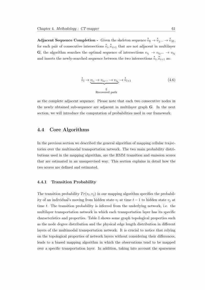
Chapter 4. Methodology : CT-mapper 61
Adjacent Sequence Completion - Given the skeleton sequence ∗v0 →
∗v1... →
∗vM ,
for each pair of consecutive intersections ∗vi,
∗vi+1 that are not adjacent in multilayer
G, the algorithm searches the optimal sequence of intersections vi1 → vi2 ... → vik
and inserts the newly-searched sequence between the two intersections ∗vi,
∗vi+1 as:
∗vi → vi1 → vi2 ... → vik︸ ︷︷ ︸ → ∗
vi+1 (4.6)
⇑Recovered path
as the complete adjacent sequence. Please note that each two consecutive nodes in
the newly obtained sub-sequence are adjacent in multilayer graph G. In the next
section, we will introduce the computation of probabilities used in our framework.
4.4 Core Algorithms
In the previous section we described the general algorithm of mapping cellular trajec-
tories over the multimodal transportation network. The two main probability distri-
butions used in the mapping algorithm, are the HMM transition and emission scores
that are estimated in an unsupervised way. This section explains in detail how the
two scores are defined and estimated.
4.4.1 Transition Probability
The transition probability Tr(vi, vj) in our mapping algorithm specifies the probabil-
ity of an individual’s moving from hidden state vi at time t− 1 to hidden state vj at
time t. The transition probability is inferred from the underlying network, i.e. the
multilayer transportation network in which each transportation layer has its specific
characteristics and properties. Table I shows some graph topological properties such
as the node degree distribution and the physical edge length distribution in different
layers of the multimodal transportation network. It is crucial to notice that relying
on the topological properties of network layers without considering their differences,
leads to a biased mapping algorithm in which the observations tend to be mapped
over a specific transportation layer. In addition, taking into account the sparseness

Chapter 4. Methodology : CT-mapper 62
(a) Cellular trajectory (b) CT-Mapper’s input + Real trajec-tory
(c) Phase I (Input & output) (d) Phase II input
(e) Phase II input and output (f) CT-Mapper’s input + Final output
Figure 4.5: An illustration of different phases of mapping algorithm. The Blueline in the Fig. 5(a) is the real GPS trajectory of a user and given a sequence of5 antenna base stations with the frequency of 15 min, the mapping algorithm can
retrieve the pink line in Fig.5(e)

Chapter 4. Methodology : CT-mapper 63
of cellular observations, it is a key to authorize transitions between nonadjacent in-
tersections. We propose a transition probability of moving from intersection vi to the
intersection vj that is a function of 2 given factors:
1) Edge type and average speed over each edge: each physical edge in the multilayer
graph G belongs to a layer. Moreover, only the road layer contains different types of
edges (such as highway, principal, local, etc.). We define matrix W where each element
of the matrix represents a weight between two nodes if there exists an interconnection
between them. The weight of each link is defined as the inverse of average speed that
one could have over the corresponding edge. Table 4.2 represents the weight according
to average speed over the edges of graph G.
Wij =
{wij if vi, vj are adjacent in G
0 otherwise.(4.7)
value of wij Condition1/10 Ψ(vi) = Ψ(vj)1/100 Ψ(vi) = Ψ(vj) = train1/80 Ψ(vi) = Ψ(vj) = metro1/90 Ψ(vi) = Ψ(vj) = road (highway)1/60 Ψ(vi) = Ψ(vj) = road (principale)1/40 Ψ(vi) = Ψ(vj) = road (regional)1/30 Ψ(vi) = Ψ(vj) = road (local)
Table 4.2: Edge classification and weights for multilayer transportation networkG.
2) Edge length: involving edge length in the transition probability, indirectly considers
higher probability for the nodes close to each than that for farther ones.
The transition probability between two intersections vi and vj is defined as the inverse
of the shortest path cost between vi and vj :
Tr(vi, vj) =
∑∀ (mn) ∈ SPvivj
wmn × d(vm, vn)
−1
(4.8)
where (mn) is an edge between vm and vn belonging to SPvivj , the shortest path
between two nodes vi and vj in graph G. The shortest path cost of SPvivj is the sum
of distances over each edge (mn) belonging to SPvivj , weighted by wmn. d(vm, vn) is

Chapter 4. Methodology : CT-mapper 64
the euclidean distance between each two nodes vm and vn.
In earlier studies, the transition probability was quantified based on topological prop-
erties of the underlying network which was mainly a road graph. In [58, 80], the trans-
portation network was represented as road segments and transitions were assumed to
occur between adjacent road segments. The authors in [44, 80] considered equal tran-
sition probabilities between nodes in the same road segment or nodes between road
segments which are adjacent with an intersection. The transition probability in [79] is
defined based on the Manhattan distance between the grid cells of the road network.
The objective of our proposed transition probability model is to minimize the bias of
the mapping algorithm for layers with different topological properties.
4.4.2 Emission Probability
In HMM, at each time step t, there exists an observation ot which in our study is
characterized as ct =< lon, lat, rmaxt >t. The emission score reflects the notion that it
is more likely that a particular observation point is observed from a nearby intersection
than an intersection farther away [80]. For studies in which GPS data were used
as observations [22, 58, 80], the emission probability score is modeled by a normal
distribution that is a function of the euclidean distance between the observation point
and the hidden state, and with a standard deviation estimated from sensor errors.
In this work, cellular antenna locations serve as observations; Since there is no labeled
data available to estimate cellular sensor errors, we build the voronoi tessellation of
cellular antennas in the area of study. In the voronoi network of cellular antennas,
each cellular antenna Ci is characterized by radius ri which is the maximum distance
of the cellular antenna from the corresponding voronoi cell vertices. Our emission
score is defined as a decreasing function of the distance between the antenna location
and the hidden node (intersection):
Pr(ot|vj) ∝
1.0 if : dtj ≤ rmax
t(rmaxt
dtj
)β
if : rmaxt ≤ dtj ≤ τ
0 otherwise.
(4.9)
where dtj = d(ot, vj) is the euclidean distance between ot and intersection vj , and τ
is a threshold corresponding to the maximum distance that a cell phone can be hit

Chapter 4. Methodology : CT-mapper 65
by a cellular antenna. τ enforces the constraint that only intersections in the radius
of τ from the cellular antenna could be considered as candidate states (nodes).
4.5 Discussion & Conclusion
This chapter covers the body of our proposed methodology, an unsupervised mapping
algorithm (CT-Mapper) designed and developed to map sparse cellular trajectories
over a multimodal transportation network. The unsupervised mapping algorithm is
designed using Hidden Markov Model properties and Viterbi decoding algorithm was
employed to infer the most likely path of the individuals given wholly sparse cellular
trajectory. The mapping algorithm is designed in a way that it takes into account
changing between different transportation layers. We modeled and built the multi-
layer transportation network database including subway, train and road layers for the
Ile-de-France metropolitan area. The multilayer transportation network enables the
mapping algorithm to retrieve the trajectories involved with more than one trans-
portation layer. Investigating the complexity of the multilayer transportation graph,
a transition probability model leveraging the transportation layer type and topolog-
ical properties was estimated and used in the unsupervised HMM-based mapping
algorithm. The emission probability is formed with respect to the noisy cellular ob-
servations. In addition, since investigating the behavior of noisy cellular observations
to infer the emission probability model is a highly data dependent task, a smoothed
emission score is derived to quantify the emission score.
The CT-Mapper is designed to map the sparse cellular trajectories over the multilayer
transportation network in two phases: The first phase infers the most likely sequence
of the nodes given only sparse cellular observations (e.g. sampled each 15 minutes) and
returns the skeleton sequence as the result. Eventually, the second phase retrieves the
complete path on the multilayer transportation network given the skeleton sequence
and returns the most likely path associated to the cellular trajectory. The main
strength of this approach is that all the steps are designed and performed in an
unsupervised way as no labeled data are required to train the model. Subsequently, we
can deploy the algorithm in large scale without manual intervention associated with
human labeling. Moreover, by injecting new knowledge from either transportation
systems or geospatial properties of the cellular antenna, the algorithm performance
can further be improved. To the best of our knowledge, this is the first attempt to

Chapter 4. Methodology : CT-mapper 66
infer multimodal trajectories of individuals over a multimodal transportation network
given only their sparse cellular data in metropolitan areas.
Along the same lines, We expect that using a dynamic weight matrix, which is com-
patible with the traffic model at different times of the day, is likely to enhance the
mapping results. This issue will be investigated in future studies. Furthermore, The
improvement of accuracy measures of our mapping algorithm by minimizing bias
mainly emanating from the multimodality of the transportation network is of great
importance which shall be discussed in future contributions. Finally, investigating
the possibility of using the proposed mapping algorithm at near real-time (NRT) for
traffic monitoring is another direction of further contributions.

Chapter 5
Mode Classification with
LCT-Mapper
5.1 Introduction
The particular advantage of studying individual trajectories over a multimodal trans-
portation network is to investigate the multimodal mobility behavior of people in
cities and urban areas. Due to the challenges of access to real, fine grain multimodal
mobility data, any insight that can shed light on these issues is extremely precious.
Investigating multimodal mobility behavior is important from different aspects: In ur-
ban planning, it helps improving the public transportation systems. In smart cities, it
can assist in detecting the major mode changing hub nodes which can lead to improv-
ing public transportation access and facilities. Human mobility studies are interested
in exploring individuals behavior in using different transportation layers. Last but
not least, it helps investigating, monitoring and predicting congestion in urban ar-
eas. However, in order to investigate large scale multimodal mobility behaviors, it
is essential to have a mechanism to obtain and perceive multimodal trajectories of
individuals. It would have involved detecting the usage of transportation modes so
that we would be able to distinguish the mode changes points. Transportation
mode inference has recently become an important issue because it can reveal valuable
insights about peoples behavior. In civil and transportation engineering fields, an
extensive study of a travel survey provided valuable information about the usage of
different transportation modes [56]. We have been inspired by this work to adapt some
definitions regarding transportation mode for our current study. It should be noted
67

Chapter 5. Mode Classification with LCT-Mapper 68
that not many studies could investigate the transportation mode detection problem
without having access to fine-grain data in metropolitan areas. Wang et al. [81]
proposed a model that uses CDRs to infer the percentage of travelers using a given
transportation mode. They used travel time distribution and clustered travelers in
different subgroups according to their travel time. Concerning individual trajectories,
researches have tried to classify transportation modes for long range trajectories [69]
[30]. The approaches above using cellular data show that inferring the transportation
mode for urban mobility and in metropolitan areas still remains a challenge.
In Chapter 4, we proposed CT-Mapper as a solution to infer the real trajectory of
smart phone users based on their sparse cellular trajectories. Since CT-Mapper is
an unsupervised estimation algorithm and does not need labeled data to infer the
parameters, it can be easily adapted for a large amount of data to infer population
trajectories. Nevertheless, it has some limitations in mode detection. As described in
4, CT-Mapper maps the sparse cellular trajectory over the multimodal transportation
network. Therefore, an inferred path can contain nodes from different transportation
network and correspondingly, deducing the transportation mode from a set of nodes
belonging to different layers is not always straightforward.The multilayer network
modeling exponentially increases the number of paths between a given source and
destination. Subsequently for a given trajectory, one can find several paths that
might be extremely similar. This complexity imposed by aggregating different trans-
portation networks, makes mapping more difficult. This chapter is focused on this
issue with the objective of proposing a solution for the problem of mode detection.
We present a solution in which we reduce the mode changing complexity by repre-
senting the multimodal transportation networks in two main class-layers. Concretely,
we propose LCT-Mapper (Layered CT-Mapper) with the supplementary objective
of uncovering if the user is on rail class-layer or he/she is on the road class-layer.
LCT-Mapper is built on with a transportation mode detection procedure augmenting
the unsupervised mapping algorithm. We first represent the multimodal transporta-
tion network in two separated class-layers, namely Rail class-layer and Road class-
layer. Then, the mapping algorithm is performed separately on each class-layer and
the result is the most likely path of the users on each class-layer associated to the
given cellular trajectory. Subsequently, the algorithm uses a classifier to choose the
best path and infer the real class-layer corresponding to the observation sequence.
LCT-Mapper provides a direct interpretation for the mode detection problem. This
interpretation is acquired by avoiding multiple changes between different transporta-
tion layers which causes errors in mode detection for CT-Mapper. To do this, we

Chapter 5. Mode Classification with LCT-Mapper 69
Figure 5.1: Instance of a trajectory in multimodal transportation network inParis and vicinity. An individual walks from origin to metro station and from metrostation to final destination (red lines) . This trajectory in mode detection problem
is considered as unimodal trajectory which is metro (blue line)
cluster the multimodal transportation network into two class-layers in which we allow
mode changing only between specific transportation layers. Domenico et al. in a
recent study [28] showed that a multiplex can be reduced to a proper proportion in
order to reduce the complexity. Inspired by this work, we reduce the multiplex of
[road+train+subway & tram] to two main clusters: rail and road networks.
In this study, we define the ’Main mode’ of a trajectory as the transportation mode
that covers the largest portion of the trajectory. Our objective, then, is to infer
the main transportation mode given a user sparse cellular trajectory. It
is worth noticing that walking is almost always part of a trajectory. This is obvi-
ous when individuals walk to and from stop stations of the public transport system,
but using the car also requires walking to and from the parking place, although the
involved distances might be short. Walking can thus be considered as a universal
component at the start and the end of any trajectory, and is therefore not considered
as a separate mode in the definition of a multimodal trip. Individuals who walk to
the bus stop, ride the bus, and walk from the stop to their destination thus make a
unimodal trajectory.
Figure 5.1 illustrates an example of real trajectory in multimodal transportation net-
work in Paris and region separated by different colors each associated to one specific
mode. The beginning and end of the trajectory consists of walking to and from the

Chapter 5. Mode Classification with LCT-Mapper 70
Mode type Mode Transportation NetworkFunctional type Carrier type
Private
Walking Pedestrain-allowed
Road
Car driving Private car-allowedBicycle riding Bicycle-allowed
Motorbike Motorbike-allowedTaxi Taxi allowed
Public
Bus taking Bus lineUnderground train Underground line
RailwaySuburban train Suburban lineTram train Tram line
Table 5.1: Transportation Modes and Networks [54]
subway station. This trajectory is considered unimodal and the objective is to infer
the main mode which in this example is subway.
The rest of this chapter is organized as follows: section 5.2 presents the mapping
algorithm framework with emphasis on the novel additional mode classifier component
of LCT-Mapper. Subsequently, section 6.5 provides the evaluation results to assess the
efficiency of our proposed approach compared to previous models and under different
circumstances. Then we discuss the obtained results and conclude the chapter.
Figure 5.2: Mapping Cellular trajectory over 2 class-layers with a classifier to chose thebest match among the two likely path

Chapter 5. Mode Classification with LCT-Mapper 71
5.2 LCT-Mapper System Overview
This section starts with problem statement in which we formulate the objective ad-
dressed in the previous section. Then, we present the framework of LCT-Mapper
with emphasis on the supplementary element of the mapping algorithm which is the
class-layer classifier. Since LCT-Mapper is the ameliorated version of CT-Mapper, for
the common components of the algorithm, we refer to chapter 4 where CT-Mapper
has been elaborated in details.
5.2.1 Problem Statement
This section contains basic mathematical definitions that are required to formulate
the problem.
Definition 1. Multilayer Transportation Graph - We define graph G = (V,E, L,Ψ)
in which V,E are the vertices and the edges of the graph. L is the set of all considered
layers (road, train, subway, tramway). Function Ψ indicates the layer of each node
by mapping each node to a layer. Ψ : V → L in G.
Definition 2. Class-layer Graph - We define the Class-layer graphs GRoad and
GRail as road class-layer and rail class-layer where:
GRoad ⊂ G, and ∀ vi ∈ GRoad, Ψ(vi) = {Road}
GRail ⊂ G, and ∀ vj ∈ GRail, Ψ(vj) = {train|subway|tram}
Each class-layer is a connected component, a subset of multimodal transportation
graph G. In other words, we split the multimodal transportation network into two
main class-layers.
Definition 3. Cellular Network - As described in section 4.3.1, the cellular net-
work is defined as the set of cell towers C = {c0, c1, ...cP }, where each cell tower
cp =< lat, lon, rmax >p is characterized by its latitude and longitude in the geograph-
ical coordinate system and by rmax that is the maximum distance of the center of the
voronoi cell from its corners. Please note that the location of each cell tower usually
does not coincide with the location of any intersection in the transportation network
i.e., ∀vi ∈ V , ∀cp ∈ C, we have < lat, lon >p = < lat, lon >i.

Chapter 5. Mode Classification with LCT-Mapper 72
Definition 3. Sparse Cellular Trajectory As defined in chapter 4, a sparse cellular
trajectory of a user is defined as O = o0 → o1... → oM and each time-stamped location
ot =< c(t) > refers to the specific antenna cell at time-stamp t.
Trajectory Mapping and Mode Classification Problem - Given the transporta-
tion network containing two class-layers G = {GRoad, GRail}, the cellular network C,
and a user sparse cellular trajectory O, the search problem is to find a sequence of in-
tersections v0 → v1... → vq as the most likely path and the associated transportation
mode associated with the retrieved path.
5.2.2 Algorithm Framework
The fundamental features of LCT-Mapper that enables it to outperform CT-Mapper
are:
I) To split the multimodal transportation network into class-layers.
II) Applying a classifier to determine the best match among the two likely paths each
associated to a class-layer.
Given the transportation network G = {Groad, GRail}, the cellular network C and a
user sparse cellular trajectory O, the mapping algorithm determines the most likely
path over each of the two class-layer Groad and GRail. As mentioned, the core of map-
ping algorithm in LCT-Mapper is implemented as the same manner of CT-mapper.
This core algorithm explained in section 4.3.4, is designed in two main phases:
Skeleton Sequence Search - In the first phase, the Viterbi decoding algorithm
is applied to find the most likely sequence of nodes separately for each class-layer
. Given the cellular trajectory o0 → o1, ... → oM , the result for this phase is two
separated sequences:
1) Road class-layer skeleton sequence v0 → v1, ... → vM where ∀vi,Ψ(vi) = {Road}
2) Rail class-layer skeleton sequence v′0 → v′1, ... → v′M where ∀v′i,Ψ(v′i) = {Rail}
Notice that in this step, there are trajectories for which the rail class-layer skeleton
sequence is empty {}. This case happens when the trajectory takes place in an area
which is not covered by the rail class-layer. (As pointed out in chapter 3, the area of
study in our work is Paris an vicinity and we showed that not all the area is covered
by the rail transportation layer.

Chapter 5. Mode Classification with LCT-Mapper 73
Adjacent Sequence Completion - The two class-layer skeleton sequences serve as
the input of the second phase to obtain the complete sequence of nodes where each two
consecutive nodes in the sequence are adjacent in their associated class-layer. Given
the skeleton sequence ∗v0 → ∗
v1... →∗vM , for each pair of consecutive intersections
∗vi,
∗vi+1 that are not adjacent in class-layer GRoad, the algorithm searches the optimal
sequence of intersections vi1 → vi2 ... → vik and inserts the newly-searched sequence
between the two intersections ∗vi,
∗vi+1 as:
∗vi → vi1 → vi2 ... → vik︸ ︷︷ ︸ → ∗
vi+1 (5.1)
⇑Recovered path
as the complete adjacent sequence. Please note that each two consecutive nodes in
the newly obtained sub-sequence are adjacent in multiplex GRoad. It is important to
notice that the same procedure is performed for both class-layers. Consequently, at
the end of this step, the results are two sequences of adjacent nodes, one associated
to GRoad and one for GRail.
The two inferred paths as illustrated in figure 5.2 serve as the input of the Class-
Layer Classifier which selects the best match for the given cellular trajectory among
the most likely paths. In the following section it is explained how the Class-Layer
Classifier performs.
5.2.2.1 Class-Layer Classifier
As mentioned, the foremost improvement of LCT-Mapper is the classifier to determine
the correct class-layer for a given cellular observation. Accordingly, the parameters of
the classifier play a key role in algorithm performance. The classifier takes as input
the two likely paths that each one is the result of mapping algorithm on the class-layer
GRoad or GRail.
Definition - We define proad as the likely path on GRoad and prail as the likely path
on GRail, we also define lroad as the length of the likely path proad on the GRoad.
Accordingly, lrail will be the length of prail on the GRail.
Classification Problem - Given two likely paths proad and prail with lroad and lrail
as their lengths, and cellular trajectory O, the classifier selects one of the paths as
the best match for the cellular trajectory O.

Chapter 5. Mode Classification with LCT-Mapper 74
In designing the classifier, there are several parameters that can be considered in the
classification problem, such as stretch factor [17] and similarity between cellular tra-
jectory and obtained skeleton similarity. Following, we elaborate on these parameters
and how they can be employed in the classifier.
• Stretch Factor. The stretch factor is defined as the ratio of the actual distance
traversed on a given trajectory to that of the shortest distance between the origin
and destination [31]. Using the mathematical definition of stretch factor [68]
in class-layer selection, the classifier selects the class-layer which its associated
likely path has smaller stretch factor:
L = arg min∀ i∈class−layer
dpi(x, y)
dGi(x, y)(5.2)
dpi(x, y) is the length of the most likely path between x and y inferred by the
mapping algorithm on class-layer Gi and dGi(x, y) is the length of shortest path
between x and y over class-layer i.
• Similarity Scores - The second approach to select the best match among
the two class-layers is to compare the two most likely paths with the cellular
trajectory. For the comparison, we propose two different metrics:
1. Root Mean Square Error (RMSE) for a set of points is the square root of
the average of squared differences between each two compared points.
RMSE =
√√√√ 1
n
n∑i=1
(xi − xi)2 + (yi − yi)
2 (5.3)
Using RMSE for class-layer selection means that the most likely path with
minimum RMSE between skeleton points and cellular observation is se-
lected as the best match:
L = arg min∀ i∈class−layer
RSME (5.4)
2. Path length similarity - Using length similarity between the most likely
path and cellular observation, the class-layer whose most likely path has

Chapter 5. Mode Classification with LCT-Mapper 75
closer length to the cellular trajectory length is selected as the best match.
L = arg min∀ i∈class−layer
|lc − lri | (5.5)
The classifier then returns the selected class-layer as the best match and sets its
associated most likely path as the inferred most likely path.
5.3 Discussion
The previous section outlined the framework of the classifier and listed the potential
parameters that classifier can use for classification task. These parameters are probed
independently, nevertheless all can be employed in an aggregation function to derive
a fuzzy classifier that also assigns a degree of certainty to the final result.
Our proposed approach presented in LCT-Mapper can raise a question that what
about the precision and information lost that result endures. It is worth to recall
that cellular signalization data used in this study, offer a novel level of temporal and
spatial granularity which is not as accurate as fine-grain mobility data such as GPS
location data. Besides, sampling rate of 15 minutes for cellular observation, prevents
us from fine-grain investigation to extract detailed sub-trajectories of an individual
during a trajectory.
In addition, taking into consideration the temporal sparsity of cellular trajectories
with the spatial resolution of antenna level, it is fair that differentiating between
private cars and taxis or identifying the mode change from riding a bus to walking
to or from a point is problematic. However deriving an approach that distinguishes
the main transportation mode between (road, train and metro) is an outstanding
attainment.
5.4 Conclusion
In this chapter we proposed LCT-Mapper by improving the mapping algorithm pro-
posed in CT-Mapper to detect the main transportation mode of trajectories with a
fair accuracy. This refinement obtained by separating the multimodal transportation
network into two class-layers and designing a classifier which distinguishes the best
match among the two most likely inferred paths.

Chapter 5. Mode Classification with LCT-Mapper 76
Splitting the multiplex transportation network into two class-layers, namely Road
and Rail class-layers, reduces the complexity of multiplex network. Moreover, this ap-
proach enables us to obtain a straightforward solution for the mode detection problem.
Nevertheless, this separation imposes a specific limitation into the mapping problem
which can be mentioned as disadvantage of this approach. Since the classifier selects
one of the two class-layers, loosing some precision in mapping is unavoidable. This
can be accepted as a satisfactory compromise given the limited spatial resolution of
the cellular data.
It is expected that this method provided efficient solution for the problem of trajec-
tories’ main mode inference. In the next chapter, the results of this algorithm are
evaluated and will be compared with the result of CT-Mapper in both, trajectory
mapping and trajectory mode detection. In case of a fair trade-off between the two
objectives, meaning the mapping algorithm from one side and the mode inference
problem from another side, this methodology with respect to the unsupervision of all
the steps, can be considered as a precious approach to analyze the cellular mobility
data in large scale.
Considering the spatial resolution of cellular observations along with the temporal
sparsity of data [which in our study is not as sparse as CDRs but less frequent than
GPS track (1-2 minutes)] induces a novel level of spatial scale for efficient study
of trajectories. This novel scale in current study was obtained by partitioning the
multimodal transportation network into ’Road’ and ’Rail’ class-layers. This approach
leads to an efficient solution for sparse cellular trajectory mapping by restricting the
mode changing actions.

Chapter 6
Algorithms Validation
6.1 Introduction
In this chapter, we present the experiments carried out to validate our proposed
model, and we provide analysis tools to assess the model’s effectiveness in reaching
the stated objectives.
In the previous two chapters, two mapping algorithms, the so-called CT-Mapper and
LCT-Mapper, were proposed to map cellular trajectories over the multimodal trans-
portation network and to infer the main transportation mode of users. As stated
previously, the two proposed methods are based on unsupervised inference models in
which no labeled data are used for training the models. As described in chapter 3,
two datasets have been collected for the sake of evaluation and validation:
1. Cellular sparse trajectories, provided by French telecom company, from a group
of volunteers during 1 month. This dataset was obtained by sampling the cellular
location of users with a frequency of 15 minutes. The test dataset contains 80
trajectories (section 3.2)
2. GPS data for the participants have been collected to serve as ground truth for
the evaluation procedure. (section 3.3)
Figure 6.1 illustrates an example of the result provided by the CT-Mapper mapping
algorithm (colored in orange) along with the GPS trajectory that is colored in blue.
Although visualization of the mapping results may be seen as an approach to eval-
uate the overall quality of mapping algorithms, quantitative measures are required
77

Chapter 6. Algorithms Validation 78
in order to objectively assess the performance of the latter. For a comprehensive as-
sessment of the performance of mapping algorithms, we use a set of metrics, namely,
sequence similarity score, Recall, Precision and F-measure. Furthermore, to evaluate
both phases of the mapping algorithm, we evaluate separately two results : skeleton
sequence similarity and complete sequence similarity. The next section provides a
brief description of these measures. Subsequently, we present the result of computing
different metrics for our obtained results. In order to establish validity of our proposed
algorithm, we also derive a baseline algorithm and an extensive set of comparison have
been performed between baseline model and our proposed models using evaluation
metrics.
Before explaining the evaluation metrics, some description regarding the experiments
is necessary.
- The result of the mapping algorithm for each trajectory is a path on the multimodal
transportation network.
- To obtain the ground truth, collected GPS data have been mapped over the same
multimodal transportation network.
- Despite the fact that GPS fine-grained data and cellular sparse trajectoreis are
mapped over the same transportation network, comparing fain-grained GPS data
with result of noisy cellular data mapping without considering any authorized error,
raises some critics. Correspondingly, we use ( Root Mean Square Errors) as a measure
to use as threshold to find the match points. Following, we briefly explain how we
employed different accuracy measures for evaluation and validation purpose.
6.2 Metrics For Performance Evaluation
6.2.1 Root Mean Square Error
Root Mean Square (RMS) Error is the difference between the desirable point (ground
truth) and the inferred point. Mathematically the RMS error is:
RMS error =√
(x− x)2 + (y − y)2 (6.1)
where (x, y) is the ground truth coordinates and (x, y) is the output coordinate.
Similarly, the Root Mean Square Error (RMSE) for a set of points presented in equa-
tion 6.2 is the square root of the average of squared differences between collected

Chapter 6. Algorithms Validation 79
Figure 6.1: CT-Mapper’s result in orange and GPS trajectory is the blue line.The two trajectories are compared using different evaluation metrics.
coordinates and coordinates from an independent source of higher accuracy ("ground
truth") for identical locations.
RMSE =
√√√√ 1
n
n∑i=1
(xi − xi)2 + (yi − yi)
2 (6.2)
It is a frequently used measure of the differences between values (Sample and popu-
lation values) predicted by a model or an estimator and the values actually observed.
The use of RMSE makes a general purpose error metric for numerical predictions.
Compared to the similar Mean Absolute Error, RMSE amplifies and severely pun-
ishes large errors.
In our evaluation, the RMS error has been used for two purposes:
1. The first one is to quantify the overall distance between the algorithm result
and the real GPS trajectory as ground truth. Figure 6.2 illustrates an example
of two trajectories, where the red line is the real trajectory and the blue line is
the algorithm result. Considering the different points (marked in blue and red
markers), the RMS error is calculated using equation 6.2.
2. The second purpose is to use RMS error to detect matches between 2 points
using threshold ϵ. In this case, if the RMS error between two points is smaller

Chapter 6. Algorithms Validation 80
Figure 6.2: Example of using RMSE for comparing two trajectories
than ϵ, we consider the inferred point as a match (using equation 6.1). Figure
6.3 shows an example illustrating an error between the inferred path and the
real path. If the RMS error between two points is smaller than ϵ, the inferred
point will be considered as a match; otherwise, it will be a miss-match for the
source point.
6.2.2 Edit Based Similarity Score
In order to evaluate the proposed mapping algorithm, we need to assess how simi-
lar are the Cellular trajectory mapping result to the ground truth GPS trajectories.
Similarity score sim(x, y) quantifies the similarity between x, y where x and y are
two sequences. It is important to take into consideration that the two sequences are
not necessarily from the same length. Thus, we use Edit distance [23] which is so
named because it can also be thought of as the minimum number of edits (insertions,
deletions, and substitutions) needed to transform one sequence into the other. The
flexibility of Edit Distance is that it is possible to give different cost to different types
of edits and it can be employed to compare sequences of two different length. In
addition it is computed optimally based on dynamic programming algorithm.
Edit Distance or Levenshtein distance: The basic form, where each edit has cost 1,
is a dynamic programming algorithm that computes the distance between 2 strings x
and y). However in our case, we do not have strings of letters, but locations, so we

Chapter 6. Algorithms Validation 81
Figure 6.3: example of how RMSE can be used as a threshold, the red markershowes the ground truth and the blue marker is the inferred point. the RMS errorbetween two points is 263 meters; it means that for threashold smaller than 263meters the blu point is miss match and othervise it is a match for the point indentified
with red marker
define the costs as distance between locations. This algorithm in [82] is mentioned
as Edit distance with Real Penalty (ERP). Consequently, instead of 1, we use cost =
d(x[i], y[j]) where d is the euclidean distance between location x[i] and y[j]. Since
the algorithm uses euclidean distance, the result is a metric measure. The modified
algorithm is:
———————————————–
1. Initialize matrix M(|x|+1)(|y|+1)
2. Fill matrix: Mi,0 = d(x[i], y[1]) and M0,j = d(x[1], y[j])
3. Recursion:
Mi,j =
{Mi−1,j−1 if x[i] = y[j]
cost+min(Mi−1,j ,Mi,j−1,Mi−1,j−1) else
4. Distance: Dist(x, y) = M|x|,|y|
———————————————–

Chapter 6. Algorithms Validation 82
- Edit Similarity: 1− Dist(x, y)
max(|x|, |y|)
In conventional approach, each mismatch costs 1. In modified case, the cost of mis-
match for (x, y), is d(x, y) where d is the geographic distance between x and y.
6.2.3 Recall and Precision
Precision and Recall are the basic measures used for evaluating the results. Precision is
the fraction of retrieved instances that are relevant. Recall (also known as sensitivity)
is the fraction of relevant instances that are retrieved. Both precision and recall are
based on an understanding and measure of relevance. In simple terms, high precision
means that an algorithm returned substantially more relevant results than irrelevant,
while high recall means that an algorithm returned most of the relevant results. When
we talk about trajectories, one option is obtaining recall and precision using parameter
’length’:
Precision =Overlapped path length
Result path length(6.3)
Recall =Overlapped path length
Real path length(6.4)
One issue with these measures however, is that the result is given by one absolute value
for recall and precision, that take into account perfect local matches. For example,
in figure 6.1, although given only 5 cellular observation, the obtained result looks fair
enough, but the recall and precision obtained with equations 6.4 and 6.3 are 67% and
64% . Since the ground truth dataset comes from higher resolution, it is reasonable
to consider a permitted error in our evaluation. Accordingly, in order to be capable of
allowing an error for evaluation, we use the nodes of the graph for relevance measure
rather that the length of the trajectory. In other words, if we define a trajectory as a
sequence of nodes over the transportation graph, the aforementioned metrics can be
represented as:
Precision =Number of common (matched) nodes
Number of result nodes(6.5)

Chapter 6. Algorithms Validation 83
Recall =Number of common (matched) nodes
Number of real path nodes(6.6)
With this formulation, a given allowed error can be considered in calculating match
and mismatch between each two nodes.
6.2.4 F-Measure
the F1 score (also F-score or F-measure) is a measure of a test’s accuracy. It considers
both the precision p and the recall r of the test to compute the score: p is the number
of correct positive results divided by the number of all positive results, and r is the
number of correct positive results divided by the number of positive results that
should have been returned. The F1 score can be interpreted as a weighted average
of the precision and recall. the F1 score reaches its best value at 1 and worst at 0.
The traditional F-measure or balanced F-score (F1 score) is the harmonic mean of
precision and recall:
F1 = 2.precision. recallprecision+recall
(6.7)
6.3 Dataset for Evaluation
In order to evaluate our proposed algorithms, GPS data are used as ground truth. We
collected the cellular trajectories of 10 volunteer participants during one month (Aug-
Sept 2014) with their corresponding GPS data. The GPS data were collected with the
help of the application "Moves" [2] which was installed on participants’ smartphones.
The captured data were the sampled phone positions during user’s movements as well
as its activities classified in four different categories: ’Walking’, ’Running’, ’Cycling’
and ’Transport’. Based on this dataset, a set of prepossessing steps were performed
in order to extract trajectories mapped over the transport networks. Furthermore,
trajectories whose lengths are shorter than 5 kilometers were filtered out from the
database. Given the low sampling rate of cellular data (a data point every 15 minutes),
it is not realistic to seek recovering a trajectory that lasts less than this threshold.
The effect of this filter on the dataset distribution could be observed in Fig. 6.4a and
Fig. 6.4b.

Chapter 6. Algorithms Validation 84
(a) Trajectory Time Distribution (b) Trajectory length Distribution
Figure 6.4: Time distribution and distance distribution
Figure 6.5: Neighboring cell distance distribution
The spatial accuracy needed in order to distinguish a real mobility from noise depends
on the distance between two base stations. In order to filter out irrelevant movements,
we filtered out all the trajectories under the threshold xth such that Pr(X < xth) = q
where Pr(X) is the distribution of distance between neighboring antennas. For q =
0.97, as Fig. 6.5 shows, all the neighboring distances are less than 5 kilometers.
As a conclusion, we built a dataset of 80 cellular trajectories (sequences of base
stations) with their corresponding GPS paths mapped over a multilayer graph G. The
multilayer transportation network contains around 16000 nodes and 26000 edges. The
users trajectories covered a total distance of 2200 kilometers. The average number
of observation points in each cellular trajectory is 5.55 and the average length of a
trajectory is 26.5 kilometers.

Chapter 6. Algorithms Validation 85
Figure 6.6: CT-Mapper Result Evaluation
6.4 CT-Mapper Evaluation
6.4.1 Algorithm Performance
To evaluate our algorithm, the aforementioned labeled dataset was used for test and
evaluation. We performed CT-Mapper to map the cellular trajectories and to com-
pare the result with GPS ground truth. It is important to notice that this comparison
is performed between two trajectories which do not have necessarily the same length.
Figure 6.1 illustrates the example in which the result of the CT-Mapper mapping
algorithm (in orange) is plotted along with the GPS trajectory (in blue). To com-
pare sequences of different lengths, we used the Edit distance between two sequences,
consisting of the minimum number of single-location edits (i.e. insertions, deletions
or substitutions) required to change one trajectory into the other. A short recall
that the CT-Mapper was designed in two phases, with skeleton sequence as the result
of phase one and complete sequence as the result of phase two. We evaluate both
phases of the algorithm by calculating the edit-based similarity scores for each step.
To have a comprehensive insight, we also calculate the average recall and precision
of the mapping results. Owing to the considerable spatial noise of cellular observa-
tions, we used the RMSE (Root Mean Square Error) to identify the matched points
between retrieved locations and real trajectory locations. For example, an error of

Chapter 6. Algorithms Validation 86
0.1 kilometers indicates that for each node in the output sequence, the node is con-
sidered as a match point if it is within a 0.1 kilometer radius of its corresponding
real location. We calculated the four mentioned accuracy results (precision, recall,
skeleton and complete sequence similarity score) for a range of fixed allowed RMSE
on the obtained mapping results. The similarity scores are the complementary of the
edit distance scores. Fig. 6.6 represents the result of this evaluation. As Fig. 6.6
shows, with allowed RMSE of 200 meters, more than 50% of skeleton and complete
trajectories can be retrieved.
This is remarkable given the sparsity of the coarse grain cellular antenna positions
with respect to real user trajectory (average of 5.5 observations per trajectory in the
dataset while the average length is 26.5 km). It is important to mention that as the
frequency of cellular data collection is 15 minutes, higher performance is expected
for CT-Mapper when the sampling is carried out at higher frequency, . The average
similarity score, for a RMSE of 1 kilometer, raises to 80%. In addition, CT-Mapper
reaches a recall and a precision of around 80% when a RMSE of 1 kilometer is allowed.
In addition to the metrics mentioned above, we compute the edit distance error not
as the number of required edits, but by considering the euclidean distance as the cost
of each required edit. The average of edit distances for all trajectories in the dataset
is 0.79 kilometer.
6.4.2 Comparison with Baseline
The purpose of the baseline run is to establish the validity of the proposed model
with specified parameters. As already mentioned, in the literature there exists no
similar mapping solution that is as comprehensive as CT-Mapper and that considers
a multilayer transportation network. Accordingly, to derive a baseline model , we keep
the same framework of the mapping algorithm and attempt to validate the parameters
of the algorithm by setting baseline parameters. To do this, one approach is to use
the parameters of models that have been proposed for the mapping algorithm with
modifications to adapt to current transportation network. Baseline 1 is a simple
model that snaps each observation to the nearest node in the network to find the
skeleton and for the second phase, uses least-cost paths between them to retrieve the
full path. The result of this baseline model is compared with CT-Mapper in Fig.6.7.
To evaluate our transition probability model based on the transportation network
properties presented in eq.(4.8), we derive Baseline 2, an HMM based baseline model

Chapter 6. Algorithms Validation 87
Figure 6.7: Up-left: Precision, up-right: Recall, bottom-left is Edit-based similar-ity scores and bottom-left is the skeleton similarity score
associated with the naive assumption consisting of setting equal probabilities for all
outgoing transitions from each node (including self node transition). Under such a
model, the transition probability between two nodes vi and vj is represented as:
Tr(vi, vj) =
ki ∗∏n∈Q
kn
−1
(6.8)
where Q = SPvivj − {vi, vj} and ki is the degree of vi. This basic assumption con-
siders all the multilayer network edges on equal footing irrespective of their layer
transportation properties. Using this transition probability model, we build an HMM
in the same way as CT-Mapper was developed. We use this model as a baseline
algorithm and run it on the test dataset to compare the results with CT-Mapper.
We calculate all four performance measures for the baseline algorithm. Fig. 6.7 com-
pares the performances of the two models. As the figures show, there is up to 20%
improvement in recall using our proposed transition probability model. Also, the av-
erage edit distance of the baseline algorithm result was 1.04 kilometer which proves
that CT-Mapper performs significantly better compared to the baseline algorithm.

Chapter 6. Algorithms Validation 88
Fig. 6.8 shows the distribution of edit distance for both the baseline algorithm and
CT-Mapper.
Figure 6.8: Sequence Edist Distance
6.4.3 Multimodality Analysis
In the next step of assessing our mapping algorithm, we investigate the accuracy
of the mapping algorithm in transportation layer detection. As mentioned in sec-
tion 4.8, the complexity of multimodal mapping significantly increases owing to the
considerable topological differences between transportation layers. Since the multi-
layer transportation network provides the possibility of layer changing in any single
trajectory, the result of mapping algorithm happens to be mapped on different trans-
portation layers and some times the optimum path produced by mapping algorithm is
splitted on different transportation layers. Accordingly, to analyze the performance of
CT-Mapper in mapping on the correct layer, we calculate the recall and precision for
correct layer detection for each layer. The overall recall and precision for the whole
network is computed as the average of recall and precision for each layer, by counting
the number of correct layer detected and we show this value for different transporta-
tion layer. Fig. 6.9 shows these measures compared with the baseline algorithm. It is
important to notice that since each assumption considers specific aspect of network’s
topological properties, they might introduce a bias in the mapping problem that can
impair the result compared to the baseline. As it is shown in fig. 6.9, the overall recall

Chapter 6. Algorithms Validation 89
and precision of correct layer detection is improved in CT-Mapper compared to the
baseline algorithm.
Figure 6.9: Recall and precision in layer detection
6.5 LCT-Mapper Evaluation
The mapping algorithm with LCT-Mapper has been performed on our data set and
different accuracy measures have been computed to evaluate the efficiency of LCT-
Mapper compared to CT-Mapper and the baseline algorithm. We have investigated
different parameters for the classifier.
6.5.1 Algorithm Performance
The first measure that we compute for the sake of evaluation is the average RMSE of
trajectories for the obtained results. Figure 6.10 compares the error distribution of
LCT-Mapper compared with CT-Mapper and the baseline model. While the average
value of RMSE for CT-Mapper was 0.79 kilometer, it was reduced to 0.66 kilometer
in LCT-Mapper. To assess the efficiency of LCT-Mapper, several experiments have
been conducted to compute different evaluation metrics. Figure 6.11 illustrates all
the metrics (recall, precision, F-measure, skeleton and complete sequence similarity)
that have been computed with respect to a range of allowed values of RMSE. In order

Chapter 6. Algorithms Validation 90
to have a better perception of the improvement of LCT-Mapper compared to CT-
Mapper, we provide an extensive comparative set of experiments to clearly assess the
efficiency of LCT-Mapper.
0 1 2 3 4 5 6Root Mean Square Error (km)
0.0
0.1
0.2
0.3
0.4
0.5
0.6
0.7
0.8
Pro
bab
ilit
y
LCT-Mapper
CT-Mapper
Baseline
Error Distribution
Figure 6.10: Root Mean Square Error (RMSE) Distribition
6.5.2 Comparison with Baseline and CT-Mapper
This section provides more comprehensive results by comparing different models: we
compare the result of LCT-Mapper with CT-Mapper and the baseline model. More-
over, as mentioned in the previous section, the unsupervised classification can decide
based on different measures; We conduct a set of experiments for different parameters
of classifier to clearly determine the efficiency of LCT-Mapper under each condition.
As stated in the previous section, to plainly compare the performance of mapping
algorithm, the similarity score is computed for both phases results. Figures 6.12 and
6.13 illustrate the skeleton and complete sequence similarity scores of the LCT-Mapper
result obtained from different classification models. In all the evaluations, we consider
the value of RMSE as threshold to accept a match between the result point and the
ground truth. Following, figures 6.14, 6.15 and 6.16 represent the precision, recall and
the F-measure of the results computed to compare different mapping algorithms with
respect to a range of allowed RMSE.

Chapter 6. Algorithms Validation 91
0.0 0.2 0.4 0.6 0.8 1.0RMSE (km)
0.2
0.3
0.4
0.5
0.6
0.7
0.8
0.9
Perc
en
tag
e
Results Evaluation
Recall
Precision
F-Measure
Complete Sequence Similarity
Skeleton Similarity
Figure 6.11: Different evaluation metrics have been caculated for LCT-Mapper withrespect to a range of allowed RMSE
0.0 0.2 0.4 0.6 0.8 1.0RMSE (km)
0.2
0.3
0.4
0.5
0.6
0.7
0.8
0.9
Sim
ilari
ty S
core
Skeleton Similarity
CT-mapper
LCT-mapper (Length similarity)
LCT-mapper (RMSE)
LCT-mapper (Stretch factor)
Baseline
Figure 6.12: Skeleton similarity LCT-Mapper compared to baseline and CT-Mapper

Chapter 6. Algorithms Validation 92
0.0 0.2 0.4 0.6 0.8 1.0RMSE (km)
0.2
0.3
0.4
0.5
0.6
0.7
0.8
0.9S
imil
ari
ty S
core
Complete Sequence Similarity
CT-mapper
LCT-mapper (length similarity)
LCT-mapper (RMSE)
LCT-mapper (Stretch factor)
Baseline
Figure 6.13: Complete sequence similarity LCT-Mapper compared to baseline andCT-Mapper
0.0 0.2 0.4 0.6 0.8 1.0RMSE (km)
0.2
0.3
0.4
0.5
0.6
0.7
0.8
0.9
Pre
cisi
on
CT-mapper
LCT-mapper (Lenght similarity)
LCT-mapper (RMSE)
LCT-mapper (Stretch factor)
Baseline
Figure 6.14: Precision calculated for LCT-Mapper compared with CT-Mapper andbaseline

Chapter 6. Algorithms Validation 93
0.0 0.2 0.4 0.6 0.8 1.0RMSE (km)
0.2
0.3
0.4
0.5
0.6
0.7
0.8
0.9
Reca
ll
CT-mapper
LCT-mapper (Lenght si;ilqrity)
LCT-mapper (RMSE)
LCT-mapper (Stretch factor)
Baseline
Figure 6.15: Recall calculated for LCT-Mapper compared with CT-Mapper and baseline
0.0 0.2 0.4 0.6 0.8 1.0RMSE (km)
0.2
0.3
0.4
0.5
0.6
0.7
0.8
0.9
F-M
easu
re
CT-mapper
LCT-mapper (Length similarity)
LCT-mapper (RMSE)
LCT-mapper (Stretch factor)
Baseline
Figure 6.16: F-measure calculated for LCT-mapper compared to CT-Mapper andbaseline

Chapter 6. Algorithms Validation 94
As the figures illustrate, among the three analyzed factors, the length similarity per-
forms better that stretch factor and RMSE measure, and then stretch factor stays
in the second place. The plots show that ’length similarity’ yet simple but effective
measure for the class-layer classifier performs better than CT-Mapper from different
aspects.
6.5.3 Mode Classification
In this section we analyze the efficiency of LCT-Mapper in mode detection. This
task in LCT-Mapper is straightforward by designing the classifier which infers the
class-layer that individuals have taken during their real trajectories. The result of
classifier is either ’Road’ class-layer or ’Rail’. We computed recall and precision of
this classifier using different parameters for the classifier. As figure 6.17 illustrates,
the unsupervised classifier can infer the class-layer associated to the main trajectory
mode with 0.83 percentage of accuracy. This performance is a significant achievement
considering that the overall mapping phases and classifier are conducted without using
any labeled data.
Figure 6.17: The performance of classifier in class-layer inference have been com-puted by two measures: Recall (R) and Precision (P) for both class-layers Rail andRaod. The Right column shows the overal accuracy of classifier that was obtained
using different factors

Chapter 6. Algorithms Validation 95
6.6 Discussion & Conclusion
In this chapter we provide an extensive range of evaluations to evaluate and validate
the two algorithms CT-Mapper and LCT-Mapper proposed in the previous chapters.
We carried experiments on a test dataset of 80 real multimodal trajectories collected
from 10 participants during one month (Aug-Sept 2014) to evaluate our algorithms.
Considering the sparsity of cellular observations (with a frequency of 15 minutes),
the percentage of retrieved paths of smartphone users is notable. To validate our
transition probability model, we compared it with a baseline algorithm that does
not take into account the transportation properties of each layer and the results
show up to 20% of accuracy improvement of the first over the second. This shows
that our transition model better accommodates the complexity of the multimodal
transportation network. Since for average speed over the edges only static values are
considered, it is expected that using a dynamic weight matrix which is compatible
with the traffic model at different times of the day, is likely to enhance further the
mapping results.
The accuracy of results obtained from different alternative parameters of LCT-Mapper
were computed and compared to CT-Mapper and to the baseline model. As discussed
previously, in spite of loosing some precision in cases where mode changing occurs be-
tween the two distinct class-layers, separating the transportation layers in two main
class-layers allows LCT-Mapper to improve the overall transportation mode detec-
tion performance. This result confirms that given limited spatial resolution, a good
compromise can be reached by trading off lost of precise multimodal trajectory infer-
ence against a better main transportation mode detection. The results also shed light
on the complexity of multimodal transportation behaviors of people in metropolitan
areas by raising questions such as: is there in reality any preference in mode chang-
ing behavior of people? Can we conclude from our obtained results whether people
tend to change modes within class-layers rather than between them? These questions
deserve more investigations to be conducted in future works. The classifier of LCT-
Mapper infers the main mode of the trajectories with around 83% accuracy. This
achievement is considerable given the fact that no labeled data were used to train
the model. Moreover, this performance is expected to be improved by injecting new
knowledge from either transportation systems or cellular sensors behaviors.


Chapter 7
Conclusion
This PhD research provides a novel solution to the high demanding problem of mul-
timodal mobility analysis of large populations in metropolitan areas. It proposes an
unsupervised mapping algorithm that maps sparse cellular trajectories over the mul-
timodal transportation network of the considered metropolitan area. We then adapt
this algorithm to propose a new solution for transportation mode detection.
This chapter summarizes the contributions of the thesis and points out its strengths as
well as its limitations. Finally, the opportunities that our research creates for further
works are presented.
7.1 Contributions
According to the objective defined in this thesis, we proposed a mapping algorithm
that maps sparse cellular data, associated with signalization data of smart phones,
over the multimodal transportation network of the considered metropolitan area. The
mapping algorithm is able to estimate the real trajectories of smart phone users over
different layers of the transportation network. To the extent of our knowledge, this
is the first attempt that considers a multimodal transportation network in an urban
area and that employs wholly noisy cellular data for the mapping algorithm.
We have used different sources of open data to create the multimodal transportation
network and to model the unsupervised mapping algorithm. The multimodal trans-
portation network database is available and is running in a MongoDB server. This
network covers the city of Paris metropolitan area (Ile-de-France), and will allow for
conducting large scale experiments when sufficient mobility data are available.
97

Chapter 7. Conclusion 98
We developed CT-Mapper, an inference algorithm that maps sparse cellular trajecto-
ries of smart phone users over the multimodal transportation network. CT-Mapper
is an unsupervised algorithm: in terms of parameter estimation and also the main
algorithm, no labeled data have been used. To the best of our knowledge, this is the
first attempt to use an entirely unsupervised algorithm for this purpose.
To validate CT-Mapper, a dataset of real multimodal trajectories has been used. We
have asked a group of volunteers and with the help of a French network operator, we
have obtained the cellular signalization data of these individuals for a period of one
month (Aug. - Sept. 2014). In parallel, another experiment has been run to collect
the associated GPS data, so that it could be used as ground truth in the evaluation
and validation phases.
Since there exists no similar algorithm for mapping noisy cellular data over a multi-
modal transportation network, we derived a baseline model by using basic assumptions
of studies mentioned in the literature. Then, extensive experiments were performed
to evaluate the performance of CT-Mapper compared to the baseline algorithm.
We also proposed LCT-Mapper that, in addition to mapping sparse cellular trajecto-
ries over the transportation network, infers the main transportation mode of trajecto-
ries. LCT-Mapper is more effective than CT-Mapper in real trajectory inference and
it performs transportation mode classification with 85% of accuracy. LCT-Mapper is
also suitable for large scale experiments as inference can be performed in parallel for
many trajectories at a time.
Comparing the mapping results between CT-Mapper and LCT-Mapper, it was ob-
served that despite its expected loss of mapping precision, the LCT-Mapper was
shown to be superior to CT-Mapper in terms of transportation mode detection. It
confirms the correctness of the compromise we make between spatial resolution and
accuracy of mapping algorithm. Nevertheless, this observation deserves further inves-
tigations in future studies.
7.2 Limitations
To meet the objective of this thesis, we made several choices in terms of the method-
ology we applied and the usage of the data related to the research context. Despite
the satisfactory results that we obtained, there are some limitations as follow:

Chapter 7. Conclusion 99
• Cellular Mobility Data - Network operators are strict about using mobility
data of users and specifically regarding their privacy. The privacy issue brought
barriers for data collection for large scale identified users. As a result, we ended
up with a small data set.
• Data Sampling Rate - In this study, sparse cellular trajectories with the fre-
quency of 15 minutes were collected. In case of using cellular data with higher
frequency (e.g. 5 minutes), considering the noisiness of the cellular data, ob-
taining higher accuracy can be expected.
• Trajectory Length Constraints - A direct consequence of temporal sparsity
of cellular trajectories, is the constraints that it imposes on the study as short
trajectories cannot be analyzed with our proposed mapping algorithm. Assum-
ing the frequency of 15 minutes for data sampling, an individual in a car or
on a train, can be relocated for distances more than 5 or 10 kilometers in a
period between two consecutive time stamps. As a result this approach may
not correctly retrieve short trajectories. We believe that a higher frequency of
cellular data sampling can relax this constraint.
• Noisy cellular data - The behavior of cellular observations are not well inves-
tigated and unlike GPS localization data type, no model have been defined for
cellular localization error. Since inferring the emission score from real data is
highly data-dependent, we expect that emission score for the mapping algorithm
can be improved with a bigger data set for cellular data.
7.3 Future Directions
Following the limitations mentioned in the previous section, we consider some direc-
tions as perspectives for this study:
• This work can be improved by using labeled data sets to improve the emission
and transition scores. Since manual labeling is a strenuous task, we are inter-
ested in approaches that provide labeled data which does not require this heavy
task. To do this, we offer a solution to motivate individuals to get involved in
the process of data labeling. This motivation to contribution has to bring some

Chapter 7. Conclusion 100
value to users and we believe a mobile application can be proposed to provide
such a value.
• In this PhD study, we modeled and developed a tool that employed cellular
mobility data, which is suitable for large scale experiments. In case of hav-
ing access to a large data set of cellular mobility data, treating such a large
amount of data requires developing parallel computing. Similarly, in case of
using streaming data for traffic monitoring purposes, providing a near real time
monitoring system dealing with streaming data becomes fundamental.
• Moreover, the thesis creates opportunities for further researches and works by
raising the following questions:
- Do people have specific preferences in using different transportation networks?
- Are these behaviors observable from individuals inferred trajectories?
- Can the multimodal mobility behavior of individuals help define the multi-
modal mobility models?
The answers to these questions shed light on many issues regarding the multi-
modal mobility behavior of user in metropolitan areas. They also help future
urban planning organizations to design and provide high performance traffic
plans and also to efficiently develop the transportation infrastructures .
• In terms of algorithm improvement, the need for more investigation in mul-
timodal transportation networks was one of the reasons behind my scientific
visit at Alephsys Lab at the "Universitat Rovira i Virgili" of Tarragona whose
activity is focused on investigating complex networks.

Thesis Contributions
• Journal Paper:
F. Asgari, A. Sultan, H. Xiong, V. Gauthier, M. El-Yacoubi. "CT-Mapper:
Mapping Sparse Cellular Trajectories to Multimodal Transportation Network".
Submitted to Computer Communications Journal.
• Patent:
V. Gautheri, F. Asgari, A. Sultan, M. El Yacoubi. "Procédé D’estimation de
Trajectoires Utilisant des Données Mobiles". Patent number: 1562736. France.
Deposed December 18, 2015
101


Bibliography
[1] Institut géographique national. http://www.professionnels.ign.fr/.
[2] Moves. https://www.moves-app.com/.
[3] Openstreetmap project. http://www.OpenStreetMap.org/.
[4] Detecting mobility patterns in mobile phone data from the ivory coast. Data for
Challenge D4D 2013, 2013.
[5] A. Abadi, T. Rajabioun, and P. A.Ioannou. Traffic flow prediction for road
transportation networks with limited traffic data. IEEE TRANSACTIONS ON
INTELLIGENT TRANSPORTATION SYSTEMS, 16(2):653–662, April 2015.
[6] R. A.Becker, R. Caceres, K. Hanson, J. M. Loh, and S. U. et al. Clustering
anonymized mobile call detail records to find usage groups. 2011.
[7] A. Aguiar, F. M. C. Nunes, M. J. F. Silva, P. A. Silva, and D. Elias. Leverag-
ing electronic ticketing to provide personalized navigation in a public transport
network. IEEE TRANSACTIONS ON INTELLIGENT TRANSPORTATION
SYSTEMS, 13(1):213–220, March 2012.
[8] M. Allamanis, S. Scellato, and C. Mascolo. Evolution of a location-based online
social network: Analysis and models. IMC ’12 Proceedings of the 2012 ACM
conference on Internet measurement conference, pages 145–158, 2012.
[9] Y. Altshuler, R. Puzis, Y. Elovici, S. Bekhor, and A. Sandy. Augmented between-
ness centrality for mobility prediction in transportation networks. International
Workshop on Finding Patterns of Human Behaviors in NEtworks and MObility
Data, pages 1–12, September 2011.
[10] D. Balcan, V. Colizza, B. Goncalves, H. Hu, and J. J. et al. Multiscale mobility
networks and the spatial spreading of infectious diseases. PNAS, 106(51):21484–
21489, 2009.
103

Bibliography 104
[11] M. Barthelemy. Spatial networks. arXiv:1010.0302, 2010. Available online:
http://arxiv.org/pdf/1010.0302v2.pdf.
[12] R. C. Basole. The value and impact of mobile information and communication
technologies. Proceedings of the IFAC Symposium, Atlanta, GA., 2004.
[13] R. Becker, R. Cáceres, K. Hanson, S. Isaacman, J. M. Loh, M. Martonosi, J. Row-
land, S. Urbanek, A. Varshavsky, and C. Volinsky. Human mobility character-
ization from cellular network data. Communications of the ACM, 56(1):74–82,
January 2013.
[14] V. D. Blondel, A. Decuyper, and G. Krings. A survey of results on mobile phone
datasets analysis. Feb 2015. DOI: 10.1140/epjds/s13688-015-0046-0.
[15] D. Brockmann, L. Hufnage, and T. Geisel. The scaling laws of human travel.
Nature, 439, January 2006.
[16] M. C.Gonzale, C. A.Hidalgo, and A.-L. Barabasi. Understanding individual hu-
man mobility patterns. Nature, 453, June 2008.
[17] S.-W. Cheng, C. Knauer, S. Langerman, and M. Smid. Approximating the av-
erage stretch factor of geometric graphs. Journal of Computeational Geometry
JoCG, 3(1):132–153, 2012.
[18] A. Clauset and N. Eagle. Persistance and peridicity in a dynamic proximity
network. DIMACS workshop on Computational Methods for Dynamic Interaction
Neworks, 2007.
[19] R. Cohen and S. Havlin. COMPLEX NETWORKS Structure, Robustness and
Function. CAMBRIDGE University Press, 2010.
[20] M. Coscia, S. Rinzivillo, and D. P. Fosca Giannotti. Optimal spa-
tial resolution for the analysis of human mobility. IEEE/ACM Interna-
tional Conference on Advances in Social Network Analysis and Mining, 2012.
DOI:10.1109/ASONAM.2012.50.
[21] B. Cs.Csajia, A. Browetc, V. Traagc, J.-C. Delvennec, E. Huensc, P. V. Doorenc,
Z. Smoredae, and V. D. Blondelc. Exploring the mobility of mobile phone users.
Statistical Mechanics and its Applications, 392:1459–1473, November 2012.

Bibliography 105
[22] C.Y.Goh, J. Dauwels, N. Mitrovic, M. T. Asif, A. Oran, and P. Jaillet. Online
map-matching based on hidden markov model for real-time traffic sensing appli-
cation. Intelligent Transportation Systems (ITSC), pages 776–781, Sept. 2012.
DOI: 10.1109/ITSC.2012.6338627.
[23] S. Dasgupta, C. Papadimitriou, and U. Vazirani. Algorithms, chapter 6, pages
169–199. McGraw-Hill, 2006.
[24] V. D.Blondel, M. Esch, C. Chan, F. Clerot, P. Deville, E. Huens, F. Morlot,
Z. Smoreda, and C. Ziemlicki. Data for development: The d4d challenge on
mobile phone data. 2012.
[25] S. Derrible. Network centrality of metro systems. PlosONE, 7(7), July 2012.
[26] L. P. S. R. D. T.-P. Dirk Koschutzki, Katharina Anna Lehmann and O. Zlotowski.
Chapter 3:Centrality Indices. Springer-Verlag Berlin Heidelberg, 2005.
[27] M. C. Dmytro Karamshuk, Chiara Boldrini and A. Passarella. Human mobility
models for opportunistic networks. Communications Magazine, IEEE, 49:157–
165, 2011.
[28] M. D. Domenico, V. Nicosia, A. Arenas1, and V. Latora. Structural reducibility
of multilayer networks. Nat. Commun., 6:6864, 2015. doi: 10.1038/ncomms7864.
[29] M. D. Domenico, A. Sole-Ribalta, E. Cozzo, M. Kivela, Y. Moreno, M. A. Porter,
S. Gomez, and A. Arenas. Mathematical formulation of multilayer networks.
Physical Review, 3, 2013. DOI: 10.1103/PhysRevX.3.041022.
[30] J. Doyle, P. Hung, D. Kelly, S. McLoone, and R. Farrell. Utilising mobile phone
billing records for travel mode discovery. 22nd IET Irish Signals and Systems
Conference, ISSC, June 2011.
[31] R. Ganti, M. Srivatsa, A. Ranganathan, and J. Han. Inferring human mobility
patterns from taxicab location traces. UbiComp ’13 Proceedings of the 2013 ACM
international joint conference on Pervasive and ubiquitous computing, pages 459–
468, 2013. http://dx.doi.org/10.1145/2493432.2493466.
[32] T. Garske, H. Yu, and Z. P. et al. Travel patterns in china. PLoS ONE, 6(2),
Feb 2011. 10.1371/journal.pone.0016364.
[33] F. Giannoti, M. Nanni, F. Pinelli, and D. Pedreschi. Trajectory pattern mining.
Proceedings of the 13th ACM SIGKDD international conference on Knowledge
discovery and data mining, pages 330–339, 2007.

Bibliography 106
[34] F. Giannotti, M. Nanni, and D. Pedreschi. Unveiling the complexity of human
mobility by querying and mining massive trajectory data. The international
Journal on Very Large Data Bases, July 2011.
[35] F. Giannotti, L. Pappalardo, D. Pedreschi, and D. Wang. A complexity sci-
ence perspective on human mobility, 2012. Available online in http://www.
dashunwang.com/pdf/2012-mobilityBook.pdf.
[36] M. C. Gonzalez, F. Simini, and A. M. andAlbert Laszlo Barabasi. A universal
model for mobility and migration patterns. Nsture, 484:96–100, 2012.
[37] P. Grindrod, M. C. Parsons, D. J. Higham, and E. Estrada. Communicability
across evolving networks. Physical Review, 83:046120, 2011.
[38] P. Holme. Congestion and centrality in traffic flow on complex network. Advances
in Complex Systems, 06:163–176, June 2003. DOI: 10.1142/S0219525903000803.
[39] P. Holme and J. Saramaki. Temporal networks. Physics Reports, 519:97–125,
October 2012.
[40] T. Hossmann, T. Spyropoulos, and F. Legendre. A complex network analysis
of human mobility. 3rd IEEE International Workshop on Network Science for
Communication Networks, April 2011.
[41] C. Hu, W. Chen, Y. Chen, and D. Liu. Adaptive kalman filtering for vehicle
navigation. Journal of Global Positioning Systems, 2(1):42–47, 2003.
[42] X. Huang and J. Tan. Understanding spatio-temporal mobility patterns for se-
niors, child/student and adult using smart card data. ISPRS - International
Archives of the Photogrammetry, Remote Sensing and Spatial Information Sci-
ences, XL-1:167–172, 2014.
[43] P. Hui and J. Crowcrof. Human mobility models and opportunistic com-
munication system design. Mathematical, Physical and Engineering Sciences,
336(1872):2005–2016, 2008.
[44] B. Hummel. Map matching for vehicle guidance, in dynamic and mobile gis:
Investigating changes in space and time. 2006.
[45] T. Hunter, T. Moldovan, M. Zaharia, S. Merzgui, J. Ma, M. J. Franklin,
P. Abbeel, and A. M. Bayen. Scaling the mobile millennium system in the cloud.
Proceedings of the 2nd ACM Symposium on Cloud Computing - SOCC ’11, pages
1–8, 2011.

Bibliography 107
[46] S. Isaacman, R. Becker, R. Caceres, and M. M. et al. Human mobility modeling
at metropolitan scales. MobiSys, June 2012.
[47] Z.-Q. Jiang, W.-J. Xie, M.-X. Li, and B. P. et al. Calling patterns in human
communication dynamics. PNAS, 110(5):1600–1605, January 2013.
[48] H.-H. Jo, M. Karasai, J. Karikiski, and K. Kaski. Spatiotemporal correlation of
handset-based service usages. EPJ Data Science, 1(10), 2012.
[49] M. Kakihara and C. Sorensen. Expanding the ’mobility’ concept. SlGGROUP
Bulletin, 22(3), 2001.
[50] C. Kang, S. Sobolevsky, Y. Liu, and C. Ratti. Exploring human movements
in singapore: A comparative analysis based on mobile phone and taxicab us-
ages. Proceedings of the 2nd ACM SIGKDD International Workshop on Urban
Computing, Audust 2013. doi:10.1145/2505821.2505826.
[51] J. Krumm. Inference attacks on location tracks. Proceedings of the 5th interna-
tional conference on Pervasive computing, pages 127–143, 2007.
[52] R. Kumar and J. Saramaki. Path lengths, correlations, and centrality in temporal
networks. Phys. Rev. E 84, 2011.
[53] K. Lerman, R. Ghosh, and J. H. Kang. Centrality metric for dynamic net-
works. MLG ’10 Proceedings of the Eighth Workshop on Mining and Learning
with Graphs, pages 70–77, 2010.
[54] L. Liu. Data Model and Algorithms for Multimodal Route Planning with Trans-
portation Networks. PhD thesis, Technical University of Munich (TUM), January
2011.
[55] M. Y. Mun, D. Estrin, J. Burke, and M. Hansen. Parsimonious mobility classi-
fication using gsm and wifi traces. HotEmNets’08, ACM, January 2008.
[56] R. V. Nes. Design of multimodal transport networks : a hierarchical approach.
PhD thesis, Technical University of Delft (DUP), January 2002.
[57] M. E. J. Newman. The structure and function of complex networks. 2003.
[58] P. Newson and J. Krumm. Hidden markov map matching through noise and
sparseness. Proceedings of the 17th ACM SIGSPATIAL International Conference
on Advances in Geographic Information Systems, pages 336–343, 2009. DOI:
10.1145/1653771.1653818.

Bibliography 108
[59] A. Noulas, alvatore Scellato, R. Lambiotte, M. Pontil, and C. Mascolo. A tale
of many cities: Universal patterns in human urban mobility. PLoS ONE, 7(5),
May 2012. doi:10.1371/journal.pone.0037027.
[60] J. P.Bagrow and Y.-R. Lin. Mesoscopic structure and social aspects of human
mobility. PLoS ONE, July 2012. DOI: 10.1371/journal.pone.0037676.
[61] U. N. W. U. Prospects. Worlds population increasingly urban with more
than half living in urban areas. https://www.un.org/development/desa/en/
news/population/world-urbanization-prospects.html, 2014. [access: 10
Jul. 2015].
[62] G. Ranjan, H. Zang, Z.-L. Zhang, and J. Bolot. Are call detail records biased for
sampling human mobility? ACM SIGMOBILE Mobile Computing and Commu-
nications Review, pages 33–44, July 2012. doi:10.1145/2412096.2412101.
[63] S. Reddy, M. Mum, and J. Burke. Using mobile phones to determine transporta-
tion modes. ACM Transactions on Sensor Networks, 6(2), February 2010. DOI
10.1145/1689239.1689243.
[64] M. B. Ricardo Galloti. The multilayer temporal network of public transportat
in great britain. 2015. cea-01119006.
[65] M. Rosvall, A. Trusina, P. Minnhagen, and K. Sneppen. Networks and cities:
An information perspective. Phys. Rev. Lett., 94:028701, Jan 2005.
[66] D. Schulz, S. Bothe, and C. Korner. Human mobility from gsm data - a valid
alternative to gps? Proceeding paper at Nokia Mobile Data Challenge, June 2012.
[67] H. G. Schuster and D. Brockmann. Reviews of Nonlinear Dynamics and Com-
plexity,. John Wiley & Sons, July 2010. ISBN: 978-3-527-40729-3.
[68] Siu-erman and M. Smid. Space-efficiency for routing schemes of stretch factor
three. Journal of Parralel and Distributed Computing, 61:679–687, 2001.
[69] Z. Smoreda, A.-M. Olteanu-Raimond, and T. Couronne. Spatiotemporal data
from mobile phones for personal mobility assessment. International conference
on transport survey Methods: Scoping the Future while Staying on Track, pages
745–767, 2013.
[70] K. Sneppen, A. Trusina, and M. Rosvall. Hide-and-seek on complex networks.
EPL (Europhysics Letters), 69(5):853, 2005.

Bibliography 109
[71] E. Strano, S. Shai, S. Dobson, and M. Barthelemy. Multiplex networks in
metropolitan areas: generic features and local effects. The Royal Socierty In-
terface, September 2015. DOI: 10.1098/rsif.2015.0651.
[72] A. Sultan, F. Benbadis, V. Gauthier, and H. Afifi. Mobile data network analysis
platform. HotPlanet, 6th International Workshop on Hot Topics in Planet-Scale
Measurement, 2015.
[73] L. Sun, K. W. Axhausen, D.-H. Lee, and X. Huang. Understanding metropolitan
patterns of daily encounters. PNAS, 110(34):13334–13779, Aug. 2013. DOI:
10.1073/pnas.1306440110.
[74] L. Sun, D.-H. L. A. Erath, and X. Huang. Using smart card data to extract
passenger’s spatio-temporal density and train’s trajectory of mrt system. Urb-
Comp ’12 Proceedings of the ACM SIGKDD International Workshop on Urban
Computing, pages 142–148, 2012. DOI: 10.1145/2346496.2346519.
[75] L. Sun, J. G. Jin, K. W. Axhausen1, D.-H. Lee, and M. Cebrian. Quantify-
ing long-term evolution of intra-urban spatial interactions. The Royal Society
Interface, 12 (102), 2014. DOI: 10.1098/rsif.2014.1089.
[76] J. Tang, M. Musolesi, C. Mascolo, and V. Latora. Temporal distance metrics for
social network analysis. in Proceedings of the 2nd ACM SIGCOMM Workshop
in online Social Networks (WOSN09), 2009.
[77] J. Tang, M. Musolesi, C. Mascolo, and V. Latora. Characterising temporal dis-
tance and reachability in mobile and online social networks. ACM SIGCOMM
Computer Communication Review, pages 118–124, 2010.
[78] J. Tang, M. Musolesi, C. Mascolo, V. Latora, and V. Nicosia. Analysing informa-
tion flows and key mediators through temporal centrality metrics. In Proceedings
of 3rd Workshop on Social Network Systems (SNS), April 2010.
[79] A. Thiagarajan, L. Ravindranath, H. Balakrishnan, S. Madden, and L. Girod. Ac-
curate, low-energy trajectory mapping for mobile devices. NSDI’11 Proceedings
of the 8th USENIX conference on Networked systems design and implementation,
2011.
[80] A. Thiagarajan, L. Ravindranath, K. LaCurts, S. Toledo, and J. Eriksson.
Vtrack: Accurate, energy-aware road traffic delay estimation using mobile
phones. SenSys 09, November 2009.

Bibliography 110
[81] H. Wang, F. Calabrese, G. D. Lorenzo, and C. Ratti. Transportation mode infer-
ence from anonymized and aggregated mobile phone call detail records. 13th In-
ternational IEEE Anual Conference on Intelligent Transportation Systems, 2010.
[82] H. Wang, H. Su, K. Zheng, S. Sadiq, and X. Zhou. An effective study on trajec-
tory similarity measures. Proceeding of the Twenty-Fourth Australasian Database
Conference (ADC), 2013.
[83] P. Wang, T. Hunter, A. M. Bayen, K. Schechtner, and M. C. González. Under-
standing road usage patterns in urban areas. Scientific Reports, 2(101), December
2012. doi:10.1038/srep01001.
[84] Y. Xiao-Yang, H. Xiao-Pu, Z. Tao, and W. Bing-Hong. Exact solution of gyration
radius of an individual’s trajectory for a simplified human regular mobility model.
Chiniese Physics Letter, 28(12):120506–1, 2011.
[85] H. Xu, H. Liu, C.-W. Tan, and Y. Bao. Development and application of a kalman
filter and gps error correction approach for improved map matching. Journal of
Intelligent Transportation Systems, 14(1):27–36, 2010.
[86] X.-Y. Yan, X.-P. Han, B.-H. Wang, and T. Zhou. Diversity of individual mo-
bility patterns and emergence of aggregated scaling laws. Scientific Reports, 3,
September 2013. doi:10.1038/srep02678.
[87] J. Yuan, Y. Zheng, and X. Xie. Discovering region of different functions in a city
using human mobility and pois. ACM KDD ’12, pages 186–194, 2012.
[88] M. Zhao, L. Mason, and W. Wang. Empirical study on human mobility for mobile
wireless networks. Military Communications Conference. MILCOM 2008. IEEE,
November 2008.