initial-boundary value problems for … · of partial differential equations ... initial-boundary...

arX

iv:1

012.

1065

v1 [

mat

h.A

P] 6

Dec

201

0

Mathematical Modelling and Numerical Analysis Will be set by the publisher

Modelisation Mathematique et Analyse Numerique

INITIAL-BOUNDARY VALUE PROBLEMS FOR SECOND ORDER SYSTEMS

OF PARTIAL DIFFERENTIAL EQUATIONS ∗

Heinz-Otto Kreiss1, Omar E. Ortiz2 and N. Anders Petersson3

Abstract. We develop a well-posedness theory for second order systems in bounded domains whereboundary phenomena like glancing and surface waves play an important role. Attempts have previ-ously been made to write a second order system consisting of n equations as a larger first order system.Unfortunately, the resulting first order system consists, in general, of more than 2n equations whichleads to many complications, such as side conditions which must be satisfied by the solution of thelarger first order system. Here we will use the theory of pseudo-differential operators combined withmode analysis. There are many desirable properties of this approach: 1) The reduction to first ordersystems of pseudo-differential equations poses no difficulty and always gives a system of 2n equations.2) We can localize the problem, i.e., it is only necessary to study the Cauchy problem and halfplaneproblems with constant coefficients. 3) The class of problems we can treat is much larger than pre-vious approaches based on “integration by parts”. 4) The relation between boundary conditions andboundary phenomena becomes transparent.

1991 Mathematics Subject Classification. 35L20,65M30.

August 27th, 2009, revised August 12th, 2010.

Introduction

The theory for first order hyperbolic systems, which was developed with fluid problems in mind, is by nowrather well understood. It turned out that energy estimates via ‘integration by parts’ and characteristics arethe most important ingrediencies in the theory.

Second order hyperbolic systems often describe problems where wave propagation is dominant. In boundeddomains this leads to a large number of boundary phenomena like glancing waves and surface waves. Attemptshave previously been made to write a second order system consisting of n equations as a larger first order system.However, boundary phenomena such as glancing and surface waves correspond to generalized eigenvalues whichare not handled by the theory for first order systems. Furthermore, the resulting first order system often consists

Keywords and phrases: Well-posed 2nd-order hyperbolic equations, surface waves, glancing waves, elastic wave equation, Maxwellequations.

∗ This work performed under the auspices of the U.S. Department of Energy by Lawrence Livermore National Laboratoryunder Contract DE-AC52-07NA27344. O.E.O. acknowledges support by grants 05/B415 and 214/10 from SeCyT-UniversidadNacional de Cordoba, 11220080100754 from CONICET, PICT17-25971 from ANPCYT, and the Partner Group grant of theMax Planck Institute for Gravitational Physics, Albert-Einstein-Institute (Germany).1 Trasko-Storo Institute of Mathematics, Stockholm, Sweden.2 Facultad de Matematica, Astronomıa y Fısica, Universidad Nacional de Cordoba and IFEG, Argentina.3 Center for Applied Scientific Computing, Lawrence Livermore National Laboratory, Livermore, California, USA.

c© EDP Sciences, SMAI 1999

http://arxiv.org/abs/1012.1065v1

2 TITLE WILL BE SET BY THE PUBLISHER

of more than 2n equations which leads to many complications. In particular, the first order system must ingeneral be augmented by side conditions to guarentee that solutions of the first order system satisfy the originalsecond order system.

In this paper we describe a theory for second order hyperbolic systems based on Laplace and Fourier trans-form, with particular emphasis on boundary processes corresponding to generalized eigenvalues. Our theoryuses pseudo-differential operators combined with mode analysis, and builds upon the theory for first order sys-tems developed in [1, 2] . This approach has many desirable properties: 1) Once a second order system hasbeen Laplace and Fourier transformed it can always be written as a system of 2n first order pseudo-differentialequations. Therefore, the theory of [1,2] also applies here. 2) We can localize the problem, i.e., it is only neces-sary to study the Cauchy problem and halfplane problems with constant coefficients. 3) The class of problemswe can treat is much larger than previous approaches based on “integration by parts”. 4) The relation betweenboundary conditions and boundary phenomena becomes transparent.

The remainder of the paper is organized as follows. In section 1 we state the general problem and providesome basic definitions. In section 2 we treat in detail the fundamental problem of a single wave equation ina half-plane subject to different types of boundary conditions. In section 3 we first study two wave equationscoupled through the boundary conditions and then outline a theory for the general case of n second orderwave equations. This theory proves that all essential difficulties already occur for scalar wave equations coupledthrough the boundary conditions. Numerical experiments are presented in section 4, where we study the differentclasses of boundary phenomena for two wave equations coupled through the boundary conditions.

1. Initial-Boundary Value Problems for second order hyperbolic systems

1.1. Well posed problems

In this paper we want to consider second order systems which are of the form

utt = P0(D)u+ F (x, t), t ≥ 0, x ∈ Ω, F ∈ C∞0 (Ω), (1)

in the halfspace Ω = x1 ≥ 0,−∞ < xj <∞, j = 2, . . . , r. Here

P0(D) = A1D21 +

r∑

j=2

BjD2j , (2)

where

A1 = A∗1 > 0, Bj = B∗

j > 0,

are n× n constant matrices, u is a vector valued function with n components and we are using the notation

x = (x1, . . . , xr), D = (D1, . . . , Dr), Dj = ∂/∂xj,

ut = ∂u/∂t = Dtu, uxj= Dju.

At t = 0 we give initial conditions by

u(x, 0) = f1(x), ut(x, 0) = f2(x).

We are interested in smooth solutions which belong to L2(Ω) and satisfy, at the boundary Γ = x1 = 0,−∞ <xj <∞, j = 2, . . . , r n linearly independent boundary conditions.

Lu =: C0ut +r∑

j=1

Cjuxj= g, g ∈ C∞

0 (Γ). (3)

TITLE WILL BE SET BY THE PUBLISHER 3

Here C0, Cj are constant n × n matrices, C1 is non-sigular and, without loss of generality, we assume it to benormalised

Assumption 1.1. C1 = I.

To facilitate the use of Laplace transformation in time, we frequently assume that the initial data arehomogeneous, i.e., f1 = f2 ≡ 0. This is however no restriction, since it is always possible to change variablesin a problem with general initial data such that the initial data becomes homogeneous in the new variable.Since the Cauchy problem is well posed (see section 3.2) we can extend the definition of the forcing and theinitial data smoothly to the whole of Rr(x) and determine its solution. Then we subtract this solution from thehalfplane problem and obtain a new halfplane problem where only the boundary data do not vanish. This is avery natural procedure because all the difficulties and many physical phenomena arise at the boundary.

We now introduce some key definitions that classify the problems according to estimates one can achieve.

Definition 1.2. Consider (1)–(3) for F = 0, f1 = f2 = 0. The problem is called Strongly Boundary Stable ifthere are constants η0 ≥ 0, and K > 0 which are independent of g, such that for all η ≥ η0 ≥ 0, T ≥ 0

∫ T

0

e−2ηt(

‖u(·, t)‖2H1(Γ) + ‖ut(·, t)‖2H0(Γ)

)

dt ≤ K

∫ T

0

e−2ηt‖g(·, t)‖2H0(Γ) dt. (4)

Definition 1.3. The problem (1)–(3) is called Boundary Stable if there are constants η0 > 0, K > 0 and α > 0,which are independent of g, such that for all η ≥ η0, T ≥ 0,

∫ T

0

e−2ηt‖u(·, t)‖2H0(Γ) dt ≤K

ηα

∫ T

0

e−2ηt‖g(·, t)‖2H0(Γ) dt. (5)

Here ‖u‖2Hp denotes the norm composed of the L2-norm of u and all its derivatives up to order p. Thus (4)tells us that we “gain” one derivative while (5) says that u is as smooth as the data. The constants α, η0 arevery important. If η0 = 0, then we can choose η = 1

T for every fixed T > 0. This shows that the solution growsat most like Tα with time. If η0 > 0, then there is bounded exponential growth. This can happen when lowerorder terms are present.

The boundary estimates allow us also to obtain interior estimates. In section 2.2 we will prove

Theorem 1.4. Consider (1)–(3) with F = 0. If the problem is Boundary Stable, then we obtain interiorestimates of the form (4), (5) where ‖u(·, t)‖2H0(Γ) is replaced by ‖u(·, t)‖2H0(Ω) and α by α ≥ α+1, respectively.

If the problem is not Boundary Stable, then it is illposed.

Since we can always reduce the data such that only g 6= 0, we could restrict ourselves to this case. However,we are interested in differential equations with variable coefficients in general domains. Thus we have also todiscuss the case that F 6= 0. In particular, we have to show that the problem is stable against perturbations bylower order (first order) terms of the differential equations.

Definition 1.5. The problem (1)–(3) with f1 = f2 = 0 is called Strongly Stable if there exists η0 > 0, T > 0,K > 0 and α > 0, which are independent of g and F such that, for all η ≥ η0,

η

∫ T

0

e−2ηt(

‖u(·, t)‖2H1(Γ) + ‖ut(·, t)‖2H0(Γ)

)

dt+ η2∫ T

0

e−2ηt(

‖u(·, t)‖2H1(Ω) + ‖ut(·, t)‖2H0(Ω)

)

dt

≤ K[

η

∫ T

0

e−2ηt‖g(·, t)‖2H0(Γ) dt+

∫ T

0

e−2ηt‖F (·, t)‖2H0(Ω) dt]

. (6)

Clearly, if (6) holds, then the problem is Strongly Boundary Stable. For first order systems the classical theory(see [1,2]) tells us that also the converse is true: If the problem is Strongly Boundary Stable, then it is StronglyStable. As we will see, after Laplace and Fourier transformation we can write our problem again as a first order


system which satisfies all the conditions of the classical theory and therefore the results of that theory are alsovalid for second order systems. In particular, the problem is stable against lower order perturbations both forthe differential equations and the boundary conditions. (See Appendix of [4]).

Due to physical phenomena like glancing and surface waves, the problems for second order systems are oftenonly Boundary Stable. This leads to

Definition 1.6. We call the problem (1)–(3) Stable if it is Boundary Stable and if, for g = 0, there exists η0 ≥ 0,K > 0 and α > 0 which are independent of F such that, for all η ≥ η0,

∫ T

0

e−2ηt(

‖u(·, t)‖2H1(Ω) + ‖ut(·, t)‖2H0(Ω) + ‖u(·, t)‖2H0(Γ)

)

dt ≤ K

ηα

∫ T

0

e−2ηt‖F (·, t)‖2H0(Ω) dt. (7)

If (7) holds, then we can obtain an estimate even when g 6= 0. We split the problem into two; one with g = 0and F 6= 0 and the other with g 6= 0 and F = 0. For the first problem we obtain (7) and for the other we useTheorem 1.4.

In applications there is often a standard energy estimate, which can be obtained by integration by partsprovided that g = 0. This estimate can be written as

‖u(·, t)‖2H1(Ω) + ‖ut(·, t)‖2H0(Ω) ≤ K

[

‖u(·, 0)‖2H1(Ω) + ‖ut(·, 0)‖2H0(Ω) +

∫ t

0

‖F (·, τ)‖2H0(Ω) dτ

]

, (8)

where the constant K is independent of F . In this case we need only to show that the problem is BoundaryStable.

Theorem 1.7. The problem is Stable if it is Boundary Stable and, for g = 0, the energy estimate (8) holds.

One might be tempted to replace the requirement (7) by the weaker estimate

∫ T

0

e−2ηt(

‖u(·, t)‖2H0(Ω) + ‖u(·, t)‖2H0(Γ)

)

dt ≤ K

ηα

∫ T

0

e−2ηt‖F (·, t)‖2H0(Ω)dt. (9)

However, the definition is not stable against lower order perturbations. In section 2.3 we will give an examplewhich is algebraically Unstable, i.e., with time the solution loses more and more derivatives.

Definition 1.8. We call the problem (1)–(3) Unstable if the estimate (7) does not hold.

For first order systems the generalization to variable coefficients (and then to quasilinear equations) usesthe theory of pseudo-differential operators and requires the construction of a symmetrizer, as described in [1],which is smooth in all variables. If the problem is Strongly Boundary Stable, then, as we have mentioned above,the same construction can be used for second order systems. If the problem is only Boundary Stable, then wehave to modify the construction. This can be done but is technically somewhat complicated and the details arebeyond the scope of this paper. However, we will make the result plausible.

Since the stability against lower order perturbations is crucial for the generalization of our results to systemswith variable coefficients in general domains, we shall give a proof in section 1.2.

It is also well known that stability against lower order perturbations allows us to use “localization” todecompose an initial boundary value problem on a general compact domain into a finite number of problemswhich are either initial values problems in the whole space, or initial boundary value problems in the half space.We illustrate the technique with a simple example in one dimension.

Consider the initial boundary value problem for the wave equation on the strip

utt = uxx, x ∈ [0, 1], t ∈ [0,∞) (10)

with initial and boundary conditions

u(x, 0) = f1(x), ut(x, 0) = f2(x), B0u(0, t) = g0(t), B1u(1, t) = g1(t), (11)


where B0 and B1 are linear first order differential operators.A partition of unity of [0, 1] can be chosen as a set of three C∞ functions ϕ1(x), ϕ2(x), ϕ3(x) where ϕ1 is a

cutoff function

ϕ1(x) = 1 if x ≤ 1/4, ϕ1(x) = 0 if x ≥ 1/2.

Similarily,

ϕ3(x) = 0 if x ≤ 1/2, ϕ3(x) = 1 if x ≥ 3/4,

and

ϕ2(x) = 1− ϕ1(x) − ϕ3(x).

We now define the functions

ui(x, t) = ϕi(x)u(x, t), i = 1, 2, 3.

Clearly u(x, t) = u1(x, t) + u2(x, t) + u3(x, t) for all x ∈ [0, 1] and

uitt = ϕiutt = ϕiuxx = uixx + Li,

where

Li = −2ϕix(u1x + u2x + u3x)− ϕixx(u1 + u2 + u3),

consist only of lower order terms and has the same support as ui. Defining also f1i(x) = ϕi(x)f1(x) andf2i = ϕi(x)f2(x) we obtain that u1 solves the half line problem

u1tt = u1xx + L1, x ∈ [0,∞), t ≥ 0,

u1(x, 0) = f11(x), u1t(x, 0) = f21(x), B0u1(0, t) = g0(t).

u2 solves the initial value problem on the whole line

u2tt = u2xx + L2, u2(x, 0) = f12(x), u2t(x, 0) = f22(x), x ∈ (−∞,∞), t ≥ 0,

and u3 solves the half line problem

u3tt = u3xx + L3, x ∈ (−∞, 1], t ≥ 0,

u3(x, 0) = f13(x), u3t(x, 0) = f23(x), B1u3(1, t) = g1(t).

If the three problems for u1, u2 and u3 are well posed, then the original problem (10)–(11) is well posed.To treat variable coefficient problems one can invoke what is known as the “principle of frozen coefficients”

to replace the problem by one with constant coefficients. Heuristically, one can think that if one localizes theproblem to very small regions then the coefficients of the equation in each region are nearly constant and thebehavior of the solution is near to that of an equation with constant (frozen) coefficients. The proof of thevalidity of this requires the use of pseudo-differential theory. Here we claim the validity of this principle for ourproblem but do not go into the details.

1.2. Stability against lower order perturbations

If the problem is Strongly Boundary Stable, then it is Strongly Stable and therefore stable against lower orderperturbations. We shall now prove that the corresponding results hold for well posed problems.

Theorem 1.9. Consider the problem (1)–(3) for F = 0, g 6= 0 and change the boundary conditions (3) to

Lu = g + lu, |l| bounded. (12)

If the problem is Boundary Stable, then the same is true for the perturbed problem.


Proof. We consider lu as part of the data. Then (5) becomes

∫ T

0

e−2ηt‖u(·, t)‖2H0(Γ)dt ≤2

ηα

(

|l|2∫ T

0

e−2ηt‖u(·, t)‖2H0(Γ)dt+

∫ T

0

e−2ηt‖g(·, t)‖2H0(Γ)dt)

. (13)

By choosing η0 such that Kηα0

|l|2 ≤ 14 , we obtain an estimate also for the perturbed problem.

Theorem 1.10. Consider the problem (1)–(3) with g = 0 and change the differential equations to

utt = P0(D)u + P1(D)u + F. (14)

Here P1(D) is a first order differential operator with bounded coefficients, i.e.,

‖P1(D)u‖2H0(Ω) ≤ K1‖u‖2H1(Ω).

Assume that our problem is Stable. Then the perturbed problem has the same property.

Proof. In the same way as in Theorem 1.9 we consider P1(D)u as part of the forcing and choose η0 and αsufficiently large. Then the desired estimate follows.

Remark 1.11. One could argue that there are too many definitions. The reason for the concept of boundarystabillity is that it gives the easiest test for wellposedness. If the problem is Strongly Boundary Stable then thistest provides sufficient conditions for wellposedness. If the problem is only Boundary Stable we can use the test tofind out what kind of boundary phenomena the problem has. This knowledge is crucial in constructing numericalmethods. In the Boundary Stable case the test provides only necessary conditions; to obtain wellposedness oneneeds to show that the estimate (7) also holds. This is always true if there is an energy estimate for homogeneousboundary data.

Remark 1.12. If we do not want to distinguish between Strongly Stable and Stable, we call the problem wellposed.

2. A single wave equation

2.1. A necessary condition for well posedness

To derive necessary conditions we consider in this section the halfplane problem for the wave equation

utt = uxx + uyy + F (x, y, t), x ≥ 0, −∞ < y <∞, t ≥ 0 (15)

with initial conditions, at t = 0,

u(x, y, 0) = f1(x, y), ut(x, y, 0) = f2(x, y)

and one of four types of boundary conditions at x = 0, −∞ < y <∞ :

1) ut = aux + buy + g, a, b real, |b| < 1, a > 0.

2) ux = ibuy + g, b real, b 6= 0, |b| < 1.

3) ux = g.

4) ux = buy + g, b real, b 6= 0.

(16)


The source F and the data fj , g are compatible smooth functions with compact support. We are only interestedin solutions with bounded L2-norm and therefore we assume

∫ ∞

−∞

∫ ∞

0

|u(x, y, t)|2 dx dy = ‖u‖2 <∞ for every fixed t. (17)

We start with a test to find a necessary condition such that the problem is well posed. In this chapter andthroughout the rest of the paper, s = η + iξ denotes a complex number where η, ξ ∈ R.

Lemma 2.1. Let F = g = 0. The problem (15)–(16) is not well posed if we can find a nontrivial simple wavesolution of type

u = est+iωyϕ(x), ‖ϕ(x)‖ <∞, Re s > 0. (18)

Proof. If we have found such a solution, then

uα = esαt+iωαyϕ(αx), α > 0.

is also a solution for any α > 0. Since Re s > 0, we can find solutions which grow arbitrarily fast exponentially.

We shall now discuss whether there are such solutions. Introducing (18) into the homogeneous differentialequation (15) and homogeneous boundary conditions (16) gives us

ϕxx − (s2 + ω2)ϕ = 0, ‖ϕ‖ <∞. (19)

(19) is an ordinary differential equation with constant coefficients and boundary conditions

1) sϕ(0) = aϕx(0) + biωϕ(0), a, b real, |b| < 1, a > 0.

2) ϕx(0) = −bωϕ(0), b real, b 6= 0, |b| < 1.

3) ϕx(0) = 0.

4) ϕx(0) = biωϕ(0), b real, b 6= 0.

(20)

The general solution of (19) is of the form

ϕ(x) = σ1eκx + σ2e

−κx, (21)

where ±κ are the solutions of the characteristic equation

κ2 − (s2 + ω2) = 0, i.e., κ =√

s2 + ω2.

We fix the argument of√

by

−π < arg(s2 + ω2) ≤ π, arg√

s2 + ω2 =1

2arg(s2 + ω2).

From the general theory (also proved in Lemma A.5 in the appendix) we know that, there is a constant δ > 0such that

Reκ ≥ δ Re s.

Therefore ϕ ∈ L2 if and only if σ1 = 0. Introducing (21) into the boundary conditions gives us

1) s = −aκ+ iωb, a, b real, |b| < 1, a > 0.

2) κ = ωb, b real, b 6= 0, |b| < 1.

3) κ = 0.

4) κ = −iωb, b real, b 6= 0.

(22)


Since, by assumption, a > 0 and Reκ > 0, there are no solutions of type (18) for the first kind of boundarycondition. It is important to stress here that chosing the the wrong sign for a in the first type of boundarycondition results into an ill posed problem and no solution can be computed. The second case in (22) implies

ω2 + s2 = ω2b2, i.e., s2 = ω2(b2 − 1).

Thus there are no solutions of type (18) for |b| < 1, b real. As Reκ > 0 there are no solution of type (18) forthe third boundary condition. Finally, since Reκ > 0 and b is real, there are no simple wave solutions of type(18) for the fourth kind of boundary condition.

We have proved

Theorem 2.2. For the boundary conditions (16) there are no simple wave solutions of type (18) other than thetrivial solution u ≡ 0.

Since (19) and (22) define eigenvalue problems, we can phrase the theorem also as

Theorem 2.3. The eigenvalue problems (19) and (22) have no eigenvalues with Re s > 0.

We shall now introduce the concept of generalized eigenvalues. For that purpose we write (22) in terms ofnormalized variables.

s′ = s/√

|s|2 + ω2, ω′ = ω/√

|s|2 + ω2, κ′ = κ/√

|s|2 + ω2.

Definition 2.4. Let s′ = iξ′0, ω′ = ω′

0 be a fixed point and consider (19),(22) for s′ = iξ′0+ η′, ω′ = ω′

0, η′ > 0.

(iξ′0, ω′0) is a generalized eigenvalue for a boundary condition if in the limit η′ → 0 the boundary condition is

satisfied.

We now calculate the generalized eigenvalues. By Lemma A.7, there are no generalized eigenvalues forboundary conditions of type 1).

For boundary conditions of type 2), we need to consider

limη′→0

(√

(iξ′0 + η′)2 + ω′02 − bω′

0

)

.

As Reκ′ ≥ 0, there will be a generalized eigenvalue for boundary condition 2) if and only if bω′0 > 0 and

−ξ′20 + ω′20 = b2ω′2

0, i.e., ξ′0 = ±√

1− b2 ω′0.

Since

κ′0 =

√

−ξ′20 + ω′20 = bω′

0 > 0,

the corresponding eigenfunctions are

u = e−|bω0|x eiω0(y±√1−b2 t).

They represent surface waves which decay exponentially in x, i.e. in the normal direction away from the bound-ary. They are important phenomena in many applications (e.g. elastic wave equations).

For boundary conditions 3) and 4) ξ′0, ω′0 must satisfy the relation

ξ′0 = ±√

1 + b2ω′0, κ′0 = −iω′

0b,

and where the sign in the first relation is chosen so that ξ′0bω′0 < 0 (because Reκ′ ≥ 0.) The corresponding

eigenfunction is

u = eiω0(bx+y)e±i√1+b2|ω0|t. (23)


For boundary condition 4) (b 6= 0,) they are oscillatory in x, y, t. For boundary condition 3) (b = 0), they areconstant normal to the boundary and they are called glancing waves. They are important physical phenomena(e.g. Maxwell’s equations).

We collect the results in

Theorem 2.5. There are no generalized eigenvalues for boundary conditions of type (1). For boundary condition(2), (3) and (4) the generalized eigenvalues are given by

2) ξ′0 = ±√

1− b2 ω′0, κ′0 = bω′

0 > 0.

3) |ξ′0| = |ω′0|, κ′0 = 0.

4) |ξ′0| =√

1 + b2 |ω′0|, κ′0 = −iω′

0b, ξ′0bω′0 < 0.

2.2. Reduction to a first order system of pseudo-differential equations

The estimates obtained in this and subsequent sections are expressed in Fourier-Laplace transformed space. Itis clear that all these estimates have their counterpart in physical space (such as the estimates in the definitionsof section 1.1). To understand the relation between both types of estimates we refer to chapter 7.4 of [2] andchapter 10 of [3].

We consider (15)–(17) with homogeneous initial data. We Laplace transform the problem with respect tot, Fourier transform it with respect to y, and denote the dual variables by s, ω, respectively. For Re s > 0 weobtain

uxx = (s2 + ω2)u+ F , u = u(x, ω, s), F = F (x, ω, s), 0 ≤ x <∞, (24)

with one of the boundary conditions

1) su = aux + ibωu+ g,

2) ux = −bωu+ g,

3) ux = g,

4) ux = ibωu+ g,

(25)

and ‖u(·, ω, s)‖2 <∞.Introducing a new variable by

ux =√

|s|2 + ω2 v, (26)

we write the Fourier and Laplace transformed system as a first order system

ux =√

|s|2 + ω2M u+ F0. (27)

Here

u =

(

uv

)

, M =

(

0 1

κ′2 0

)

, F0 =1

√

|s|2 + ω2

(

0

F

)

,

withκ′ =

√

(s′)2 + (ω′)2, s′ =s

√

|s|2 + ω2, ω′ =

ω√

|s|2 + ω2.

The eigenvalues µ of M are µ1 = −κ′ and µ2 = κ′. The boundary conditions at x = 0 become

1) s′u = av + ibω′u+ g′, a > 0, |b| < 1,

2) v = −bω′u+ g′, |b| < 1, b 6= 0,

3) v = g′,

4) v = ibω′u+ g′, b real, b 6= 0,

(28)


with g′ = g/√

|s|2 + ω2.

Remark 2.6. We present in this and the following section the easiest way to obtain the estimates at theboundary and in the interior of the domain. To generalize these results to variable coefficients pseudo-differentialtheory is needed. The transformations S and T introduced below (see eqns. (30,45)) need to be smooth inthe dual variables. The smoothness condition may fail only at the double root of M. In this case the Kreiss’symmetrizer is used to get the estimates as explained in [1].

We shall now calculate the solution for the case when F = 0, and estimate it on the boundary.The eigenvector of M connected with −κ′ is given by

x =

(

1−κ′

)

. (29)

The transformation

S =

(

1 κ′

−κ′ 1

)

(30)

is, except for a trivial normalization, unitary and transforms M into upper triangular form, i.e.,

S−1MS =

(

−κ′ d0 κ′

)

, d =1 + |κ′|41 + |κ′|2 . (31)

Here S, S−1, d are uniformly bounded and depend smoothly on κ′.Introducing a new variable by

(

uv

)

= S

(

uv

)

(32)

transforms (27) into(

uv

)

x

=

(

−κ d√

|s|2 + ω2

0 κ

)(

uv

)

. (33)

As the solution is in L2, we have v = 0 and also u = u. Thus the boundary conditions become

1) (s′ + aκ′ − ibω′)u = g′,

2) (κ′ − bω′)u = −g′,3) κ′u = −g′,4) (κ′ + ibω′)u = −g′.

(34)

By (22), these boundary conditions become singular exactly at the generalized eigenvalues.

Remark 2.7. From all the boundary conditons the first one is the most benign. By Lemma A.7 we obtain theestimate on the boundary

|u(0, ω, s)|2 ≤ const.

|s|2 + ω2|g(ω, s)|2. (35)

In this case we gain a derivative on the boundary and the problem is Strongly Boundary Stable. According tothe classical theory [1, 2] the problem is Strongly Stable. Moreover, the principle of localization holds and theproblem can be generalized to variable coefficients and then to quasilinear equations. It is worth noticing herethat away from generalized eigenvalues, i.e. when the coefficients on the left hand side of (34) are strictly awayfrom zero, the estimate (35) holds also for boundary conditions 2), 3) and 4) and therefore the problem can betreated by the classical theory.

Because of the previous remark, we only need to study the estimates near the generalized eigenvalues. Wehave


Theorem 2.8. The problem (15)–(17) with F = 0 and f1 = f2 = 0 has a unique solution in L2 which,Fourier-Laplace transformed, is given by

u = e−κxu(0, ω, s), κ =√

s2 + ω2. (36)

For the different boundary conditions sharp estimates follow. For boundary condition 1) and, “away” fromgeneralized eigenvalues, for all other boundary conditions the problem is Strongly Boundary Stable and

1) |u(0, ω, s)|2 ≤ const.

|s|2 + ω2|g|2. (37)

Near generalized eigenvalues the estimates for boundary conditions 2), 3) and 4) are

2) |u(0, ω, s)|2 ≤ const.

η2|g|2,

3) |u(0, ω, s)|2 ≤ const.|g|2|κ|2 ≤ const.

|g|2η(|s|2 + ω2)1/2

,

4) |u(0, ω, s)|2 ≤ const.

η2|g|2,

(38)

and the problem is Boundary Stable.

Proof. Clearly, as v = 0 and u = u, (36) is the only solution to (33). We need to consider only a neighbourhood

of the generalized eigenvalues (iξ′0, ω′0). For the second boundary condition ξ′0 = ±

√1− b2 ω′

0, i.e.,

s′ = i(ξ′0 + ξ′) + η′, η′ ≥ 0, ω′ = ω′0 + ω′, |ξ′|+ |ω′|+ η′ ≪ 1.

Since κ′ 6= 0 at (iξ′0, ω′0), we can use Taylor expansion. A simple perturbation caculation shows that the worst

estimate occurs for ξ′ = ω′ = 0. In this case we have,

|κ′ − bω′| =∣

∣

∣

√

−ξ′20 + 2iξ′0η′ + η′2 + ω′2

0 − bω′0

∣

∣

∣

=∣

∣

∣

√

b2ω′20 + 2iξ′0η

′ + η′2 − bω′0

∣

∣

∣

≈∣

∣

∣

∣

|bω′0| − bω′

0 +iξ′0η

′

|bω′0|

∣

∣

∣

∣

≈√1− b2

|b| η′ if bω′0 > 0.

(39)

Thus we have

|u(0, ω, s)|2 ≤ const.|g′|2η′2

= const.|g|2η2

.

A similar perturbation calculation gives

|κ′ + ibω′| ≃√1 + b2

|b| η′ +O(η′2) (40)

which gives, for the last boundary condition

|u(0, ω, s)|2 ≤ const.|g|2η2

.


For the third boundary condition on can do better. Lemma A.4 with b = 0, gives us

|u(0, ω, s)|2 ≤ const.

( |g′||κ′|

)2

= const.

( |g||κ|

)2

≤ const.

η

|g|2(|s|2 + ω2)1/2

. (41)

This proves the theorem.

Theorem 2.9. When f1 = f2 = 0 and F = 0. The unique solution to our problem, described in Theorem 2.8,satisfies the following interior estimates. For boundary condition 1) and, away from generalized eigenvalues,for boundary conditions 2), 3) and 4)

‖u‖2 ≤ const.

η

|g|2|s|2 + ω2

. (42)

Close to generalized eigenvalues, for the corresponding boundary conditions, we have

2) ‖u‖2 ≤ const.

η2|g|2

(|s|2 + ω2)1/2

3) ‖u‖2 ≤ const.

η3/2|g|2

(|s|2 + ω2)3/4.

4) ‖u‖2 ≤ const.

η3|g|2

(43)

Proof. By Theorem 2.8 and Lemma A.2, the solution satifies

‖u‖2 ≤ 1

Reκ|u(0, ω, s)|2.

Since, by Lemma A.5, always Reκ ≥ δ4η, we obtain from (36) that (42) is valid. 2) follows because, by Theorem

2.5, Reκ′ ≃ bω′0 and then Reκ ≥ const.

√

|s|2 + ω2. 3) follows from (41), Lemma A.6 and Lemma A.4, accordingto

‖u‖2 ≤ const.|g|2

Reκ|κ|2 ≤ const.|g|2

η|κ|√

|s|2 + ω2≤ const.

|g|2η3/2(|s|2 + ω2)3/4

. (44)

Finally 4) corresponds to 4) of (38). This proves the theorem.

2.3. Estimates for homogeneous boundary data

We consider now the problem (27),(28) with g′ = 0 and treat only the cases 2), 3) and 4) where there aregeneralized eigenvalues (see Remark 2.7).

For η = Re s > 0, the eigenvalues of M are distinct and therefore we can transform (27) to diagonal form bythe transformation

T =

(

1 1−κ′ κ′

)

, T−1 =1

2

(

1 −1/κ′

1 +1/κ′

)

, (45)

Let u, v be defined by(

uv

)

= T

(

uv

)

. (46)

Then, (27) becomes(

uv

)

x

=

(

−κ 00 κ

)(

uv

)

+1

2κ′√

|s|2 + ω2

(

−FF

)

, (47)


with boundary conditions

2) (κ′ − bω′)u(0, ω, s) = (κ′ + bω′)v(0, ω, s).

3) u(0, ω, s) = v(0, ω, s).

4) (κ′ + ibω′)u(0, ω, s) = (κ′ − ibω′)v(0, ω, s).

(48)

The equations (47) are decoupled and as Reκ > 0, Lemma A.1 gives for all boundary conditions

|v(0, ω, s)|2 ≤ 1

8|κ′|2Reκ‖F‖2

|s|2 + ω2=

1

8|κ′|2Reκ′‖F‖2

(|s|2 + ω2)3/2,

‖v(·, ω, s)‖2 ≤ 1

4|κ′|2|Reκ|2‖F‖2|

|s|2 + ω2=

1

4|κ′|2|Reκ′|2‖F‖2

(|s|2 + ω2)2.

(49)

We use the boundary conditions to estimate u(0, ω, s).Theorem 2.5 tells us that Reκ′0 ≈ bω′

0 > 0 in a neighborhood of the generalized eigenvalue connected withboundary condition 2). Therefore the perturbation calculation (39) gives us

|u(0, ω, s)|2 =∣

∣

∣

κ′ + bω′

κ′ − bω′

∣

∣

∣

2

|v(0, ω, s)|2 ≤ const.

η′2‖F‖2

(|s|2 + ω2)3/2

≤ const.

η2‖F‖2

(|s|2 + ω2)1/2.

(50)

The interior estimate in this case follows from Lemma A.2, Reκ = Reκ′√

|s|2 + ω2 and (50)

‖u(·, ω, s)‖2 ≤ |u(0, ω, s)|2Reκ

+const.

(Reκ)2‖F‖2

|s|2 + ω2

≤ const.

η2‖F‖2

|s|2 + ω2

(51)

Since the transformation T is bounded, (46) tells us that the estimates (49)–(51) are also valid for u, v. Thusthe problem is Stable.

For boundary condition 3), the generalized eigenvalue is κ′ = 0 and therefore, for Re s′ > 0, we know onlythat Reκ′ ≥ δRe s′. However, by Lemma A.6, we have a strong estimate for |κ|Reκ and the estimates (49)become

|v(0, ω, s)|2 ≤ const.

η|κ|‖F‖2

√

|s|2 + ω2≤ const.

η2‖F‖2

√

|s|2 + ω2

‖v(·, ω, s)‖2 ≤ const.

η2‖F‖2

|s|2 + ω2.

(52)

By (48), the same estimate holds for u(0, ω, s). By Lemma A.2, we obtain the interior estimate

‖u(·, ω, s)‖2 ≤ const.

η2‖F‖2

|s|2 + ω2. (53)

Since u, v satisfy the same estimates, the problem is Stable.


For boundary condition 4), the generalized eigenvalue is κ′0 = −iω′0b, b 6= 0, is purely imaginary. Therefore,

for Re s′ > 0, we can only use the estimate Reκ′ ≥ δη′. Instead of (50) we obtain now

|u(0, ω, s)|2 =∣

∣

∣

κ′ − iω′b

κ′ + iω′b

∣

∣

∣

2

|v(0, ω, s)|2 ≤ const.

η3‖F‖2.

Again, the same estimates hold for u, v. The estimates are sharp. Therefore we do not obtain the desired interiorestimate and the problem is Unstable. We have proved

Theorem 2.10. For boundary conditions 2) and 3) our problem is Stable, but not for boundary condition 4).

Remark 2.11. The estimates obtained for boundary conditions 2) and 3) tell us that u gains one derivativewith respect to the forcing in the interior of the domain and half a derivative on the boundary. The problemcan be localized and generalized to variable coefficients and then to quasilinear equations. On the other hand,the estimates for the problem with boundary condition 4) show that not even a fractional derivative is gainedwith respect to the forcing. This, for a second order equation, means that one derivative of the solution is lostat every reflection on the boundary. The problem can not be localized. We do not pursue this problem butillustrate below this bad type of behavior with a simple example: a first order system with a boundary conditionequivalent to 4).

An example: Boundary reflection with loss or gain of differentiability. Consider a system of differentialequations

ut = −ux, vt = vx, 0 ≤ x ≤ 1, t > 0, (54)


u(0, t) = vx(0, t), v(1, t) = ux(1, t). (55)

Thenu = eλ(t−x)u0, v = eλ(t+x)v0, (56)

is a solution of (54).Introducing (56) into (55) gives us

u0 = λv0, eλv0 = −λe−λu0. (57)

Thus we obtain a solution of (54),(55) if

e2λ = −λ2. (58)

Letλ = λn = πin+ λn, n = 1, 2, . . . ,

then (58) becomes

e2λn = π2n2 − 2πinλn − λ2n. (59)

(59) has a solution

λn ≈ log πn.

Therefore the solution (56) grows like

eλt ≃ eπint · etlog πn = eπint(πn)t. (60)

If the initial data can be expanded into a Fourier series

u(x, 0) =∑

n

eλnxu(λn),

then (60) tells us that the solution loses more and more derivatives with time.


Now change the boundary conditions (55) to

ux(0, t) = v(0, t), vx(1, t) = u(1, t).

Then we obtain, instead of (58),

−λu0 = v0, λeλv0 = e−λu0,

i.e.,

e2λ = − 1

λ2. (61)

Therefore there is no loss of derivatives.Geometrically, the two sets of boundary conditions represents two different situations. In the first case any

wave loses a derivative when reflected at the boundary. In the second case, it gains a derivative.

3. Second order systems of hyperbolic equations

3.1. Two wave equations

In this section we consider two wave equations coupled through the boundary conditions.

u1tt = u1xx + u1yy, u2tt = u2xx + u2yy, (62)

on the halfplane x ≥ 0, −∞ < y <∞, for t ≥ 0, with homogeneous initial conditions

ui(x, y, 0) = uit(x, y, 0) = 0, i = 1, 2, t = 0, (63)

and boundary conditions at x = 0,

u1x + b1u2y = g1, u2x + b2u1y = g2, x = 0. (64)

Here b1, b2, are real and gj = gj(y, t), j = 1, 2, are smooth functions which are compatible with the initial data(for example, functions that vanish near t = 0). We want to show that our techniques of section 2 can still beused to describe the behavior of the solution.

Fourier and Laplace transform lead to

u1xx − (ω2 + s2)u1 = 0, u2xx − (ω2 + s2)u2 = 0, Re s > 0. (65)

Thus we obtain solutions that belong to L2

u1 = est+iωy−κxu10, u2 = est+iωy−κxu20, (66)

where

κ =√

ω2 + s2, for Re s > 0.

We recall here that Reκ > 0 when Re s > 0. The transformed boundary conditions become

−κu10 + iωb1u20 = g1,

iωb2u10 − κu20 = g2.(67)

A simple calculation shows that (67) has a unique solution

u10 = −κg1 + iωb1g2κ2 + ω2b1b2

, u20 = −κg2 + iωb2g1κ2 + ω2b1b2

, (68)


if and only if

Det

(

−κ iωb1iωb2 −κ

)

= κ2 + ω2b1b2 6= 0. (69)

There is an eigenvalue to the homogeneous problem (65), (67) with g1 = g2 = 0, if the homogeneous system(67) has a nontrivial solution. By (67), this is the case if

κ2 + ω2b1b2 = s2 + ω2(b1b2 + 1) = 0. (70)

There are five different situations:

(1) b1b2 < −1. By (70), there are eigenvalues s with Re s > 0. Therefore our problem is not well posed.(2) b1b2 = −1. Now s = 0 is a generalized eigenvalue. For s 6= 0 the solution (68) becomes

u10 = −κg1 + iωb1g2s2

, u20 = −κg2 + iωb2g1s2

. (71)

In general, we can not expect that u10, u20 stay bounded for s → 0. We need to assume that gj = gjttare the second time derivatives of smooth functions.

(3) −1 < b1b2 < 0. By (66),(70), we obtain generalized eigenvalues and eigenfunctions if s = ±i√1 + b1b2 |ω|,

κ =√

|b1b2|ω. The solution (68) is singular at the eigenvalues and u10, u20 have a first order pole. Inphysical space we obtain surface waves whose amplitudes become large for b1b2 → −1.

(4) b1b2 = 0. Now s = ±ω, κ = 0 determine the generalized eigenvalues and eigenfunctions. The behavioris the same as for the Neuman problem. We obtain glancing waves.

(5) b1b2 > 0. In this case the generalized eigenvalues and eigenfunctions are determined by s = ±i√1 + b1b2 ω,

κ = ±i√b1b2 ω. The eigenfunctions are oscillatory and the solution behaves like the solution of the wave

equation in section 2.3 with boundary condition 4). Thus it is Unstable.

In summary we can state that the problem (62)–(64) is well posed for boundary conditions 2)–4) and Unstablefor boundary condition 5). Also, there can be numerical diffculties if b1b2 + 1 is zero or close to zero.

When we study the estimates for the problem in the cases 3) and 4) we get completely analogous estimatesas the ones found for a single wave equation.

Consider the systemu1tt = u1xx + u1yy − F1, u2tt = u2xx + u2yy − F2, (72)

with boundary conditionsu1x + b1u2y = 0, u2x + b2u1y = 0, x = 0. (73)

Fourier and Laplace transform gives us

u1xx = (s2 + ω2)u1 + F1, u2xx = (s2 + ω2)u2 + F2,

and defineu1x =

√

|s|2 + ω2 v1, u2x =√

|s|2 + ω2 v2.

Thus, the first order form of the problem becomes

(

u1v1

)

x

=√

|s|2 + ω2

(

0 1κ′2 0

)(

u1v1

)

+1

√

|s|2 + ω2

(

0

F1

)

(

u2v2

)

x

=√

|s|2 + ω2

(

0 1κ′2 0

)(

u2v2

)

+1

√

|s|2 + ω2

(

0

F2

) (74)


√

|s|2 + ω2 v10 + iωb1u20 = 0,√

|s|2 + ω2 v20 + iωb2u10 = 0.


We transform (74) to diagonal form. Let

(

ujvj

)

=

(

1 1−κ′ κ′

)(

ujvj

)

, j = 1, 2.

Then

(

u1v1

)

x

=

(

−κ 00 κ

)(

u1v1

)

x

+1

√

|s|2 + ω2F1

(

u2v2

)

x

=

(

−κ 00 κ

)(

u2v2

)

x

+1

√

|s|2 + ω2F2

(75)


−κu10 + iωb1u20 = −κv10,iωb2u10 − κu20 = −κv20.

(76)

In the same way as in section 2.3 we can determine −κv10, −κv20 by solving the equations (75) for v1, v2and reduce the problem (72),(73) to the previous problem (62)–(64). Thus we obtain the same estimates.

3.2. General systems. The Cauchy problem

We consider the Cauchy problem for the homogeneous system of the introduction

utt = P0(D)u, t ≥ 0, x ∈ Rr : −∞ < xj <∞, j = 1, 2, . . . r (77)

were

P0(D) = A1D21 +

r∑

j=2

BjD2j . (78)

A1 = A∗1 > 0, Bj = B∗

j > 0, are positive definite symmetric n × n matrices and u is a vector valued functionwith n components.

At t = 0 we give initial datau(x, 0) = f1(x), ut(x, 0) = f2(x). (79)

Also, f1, f2 are smooth functions with compact support.We want to show that the problem is well posed. Fourier transform with respect to x gives us

utt = −P0(ω)u, P0(ω) = A1ω21 +

r∑

j=2

Bjω2j , P0(ω) = P ∗

0 (ω) > 0

andu(ω, 0) = f1(ω), ut(ω, 0) = f2(ω),

Introducing a new variable

ut = P1/20 v,

gives us(

uv

)

t

=

(

0 P1/20

−P 1/20 0

)

(

uv

)

.

Therefore we obtain∂

∂t

(

|u|2 + |v|2)

= 0,


i.e.

‖u(·, t)‖2 + ‖v(·, t)‖2 = ‖u(·, 0)‖2 + ‖v(·, 0)‖2.This energy estimate shows that the Cauchy problem is well posed.

3.3. The resolvent equation

Consider the Cauchy problem for the inhomogeneous system (77) with F (x, t) ∈ C∞0 and with homogeneous

initial data f1 = f2 = 0.

utt = P0(D)u+ F. (80)

Fourier transform with respect to x and Laplace transform with respect to time gives us the resolvent equation

(

s2I + |ω|2P0(ω′))

u = F , s = iξ + η, η > 0, ω′ = ω/|ω|. (81)

Since P0 = P ∗0 > 0, there is a unitary transformation which transforms (81) to diagonal form

(

s2 + |ω|2µj

)

uj = Fj , j = 1, 2, . . . , n, u = S1u, F = S1F ,

i.e.,

(s+ i|ω|√µj)(s− i|ω|√µj)uj = Fj .

Without restriction we can assume that ξ > 0. Then

|s+ i|ω|√µj | =√

|ξ + |ω|√µj |2 + η2 ≥√

|s|2 + |ω|2µj ,

|s− i|ω|√µj | =√

|ξ − |ω|√µj |2 + η2 ≥ η = Re s.

Therefore

|uj | ≤|Fj |

√

|s|2 + |ω|2µj Re s.

Choosing Im s = i|ω|√µj shows that the estimate is sharp.We have proved

Theorem 3.1. There is a constant K which does not depend on ω such that the resolvent estimate

|u(ω, s)| ≤ K|F |√

|s|2 + |ω|2Re s(82)

holds.

The last estimate shows that we ‘gain’ one derivative, i.e., if the forcing ∈ Hp, then the solution ∈ Hp+1.Therefore we can prove that the Cauchy problem is stable against lower order perturbations.

Theorem 3.2. Consider the Cauchy problem with homogeneous initial data for

utt = (P0(D) + P1(D))u+ F.

Here P1(D) represents a general first order operator. There is an η0 > 0 such that the estimate (82) holds forη = Re s > η0.


Proof. We consider P1(D)u as part of the forcing. Then (82) gives us

|u(ω, s)| ≤ K

Re s

|P1(iω, s)u|√

|s|2 + |ω|2+

K

Re s

|F |√

|s|2 + |ω|2.

Since |P1(iω,s)|√|s|2+|ω|2

is uniformly bounded, we choose η0 such that

K

η0

|P1(iω, s)u|√

|s|2 + |ω|2≤ 1

2|u(ω, s)|.

Then the desired estimate follows.

We can write the resolvent equation also as a first order system. We Fourier transform (80) with respect tox− = (x2, . . . , xr) and Laplace transform it with respect to t. Then we obtain

A1D21u =

(

s2I +B(ω−))

u− F , B(ω−) =r∑

j=2

Bjω2j , (83)

u = u(x1, ω−, s) ∈ L2(0 ≤ x1 <∞).

Since A1 > 0, there is a constant σ > 0 such that A1 = A∗1 ≥ σI > 0. Introducing a new variable by

D1u =√

|s|2 + |ω−|2 v,

we obtain the first order system

D1

(

uv

)

=M(s, ω−)

(

uv

)

+1

√

|s|2 + |ω−|2

(

0

−A−11 F

)

, (84)

where

M =M(s, ω−) =

0√

|s|2 + |ω−|2IA−1

1 (s2I+B(ω−))√|s|2+|ω−|2

0

.

The eigenvalues κ of M are solutions of

A1κ2ϕ0 =

(

B(ω−) + s2I)

ϕ0. (85)

Lemma 3.3. For Re s > 0, there are no κj with Reκj = 0. Also, there are exactly n eigenvalues, countedaccording to their multiplicity with Reκ < 0 and, therefore, n eigenvalues with Reκ > 0.

Proof. Assume there exists a κ = iω1 which is purely imaginary. Then, by (81),

(

s2I − P0(iω1, iω−))

ϕ0 = 0 (86)

has a nontrivial solution, i.e., s2 is an eigenvalue of P0(iω). P0(iω) < 0 implies that s2 is real and negative whichis a contradiction with Re s > 0.

The solutions of (85) are continuous functions of ω−. Therefore the number of κ with Reκ < 0 does notdepend on ω− and we can assume that ω− = 0. Then (85) reduces to

(s2I −A1κ2)ϕ0 = 0. (87)


Since, by assumption, A1 has positive eigenvalues µj and a complete system of eigenvectors, we can transform(87) into n scalar equations

(s2 − µjκ2)uj = 0, j = 1, 2, . . . , n,

i.e.,κ = ±s/√µj , µj > 0, j = 1, 2, . . . n, Re s > 0.

This proves the lemma.

By Schur’s lemma, there exists a unitary transformation U = U(s, ω−) such that

U∗(s, ω−)M(s, ω−)U(s, ω−) =

(

M11 M12

0 M22

)

, (88)

where the eigenvalues κj1, κj2 of M11 and M22 satisfy Reκj1 < 0,Reκj2 > 0, respectively, for Re s > 0. Clearly,the transformed equation (84) can be solved uniquely for Re s > 0.

Using (82), we shall now derive estimates for the solutions of (84). To accomplish this we consider a moregeneral forcing. We replace

1√

|s|2 + |ω−|2

(

0

A−11 F

)

by

(

F1

F2

)

, Fj = Fj(x1, ω−, s).

We Fourier transform (84) with respect to x1 and consider

iω1u =√

|s|2 + |ω−|2v − F1,

iω1v =A−1

1

(

s2I +B(ω−))

√

|s|2 + |ω−|2u− F2.

Eliminating v gives us(

s2I + |ω|2P0(ω′))

u = iω1A1F1 +√

|s|2 + |ω−|2A1F2.

Therefore, by (82), we obtain the estimate

|u(ω, s)| ≤ K|iω1F1 +

√

|s|2 + |ω−|2F2|√

|s|2 + |ω|2Re s

≤ K|F1|+ |F2|

Re s, Fj = Fj(ω1, ω−, s).

Eliminating u, we obtain the same estimate for v. Therefore we have proved

Lemma 3.4. There exists a constant K > 0 such that, for all ω1, ω−, s,

∣

∣

∣

(

M(s, ω−)− iω1I)−1∣

∣

∣ ≤ 2K

Re s. (89)

In particular, the eigenvalues κ of M(s, ω−) satisfy

|Reκ| ≥ Re s

2K. (90)

Using scaled variables

s′ = s/√

|s|2 + |ω−|2, ω′ = ω/√

|s|2 + |ω−|2, M ′(s′, ω′) =

(

0 IA−1

1

(

s′2I + β(ω′−))

0

)

, (91)


we can write (89),(90) in the form

|(

M ′(s′, ω′−)− iω′

1I)−1 | ≤ 2K

Re s′, (92)

|Reκ′| ≥ Re s′

2K. (93)

3.4. Reduction to a first order system of pseudo-differential equations

Now we consider the general halfplane problem (1)–(3) with homogeneous initial data f1(x) = f2(x) = 0,coupled to the boundary conditions (3). We Fourier transform the problem with respect to x− = (x2, x3, . . . xr)and Laplace transform it with respect to t and obtain (83) coupled to the boundary condition

ux + (C0s+r∑

j=2

Cjωj)u = g, u = u(0, ω−, s), g = g(ω−, s) (94)

As in section 2 we have to assume that there are no simple wave solutions for Re s > 0 i.e., that the eigenvalueproblem consisting of the homogeneous equations (83) and (94) have no eigenvalues s with Re s > 0, otherwisethe problem is not well posed.

Now we introduce new variables by

u = A−1/21 u1, D1u =

√

|s|2 + |ω−|2v (95)

and obtain a normalised version of (84)

D1

(

uv

)

=√

|s|2 + |ω−|2 M(

uv

)

+1

√

|s|2 + |ω−|2

(

0

−A−1/21 F

)

(96)

where

H(s′, ω′) = A−1/21

(

s′2I +B(ω′−))

A−1/2, M =

(

0 IH 0

)

,

and s′ = s/√

|s|2 + |ω−|2, ω′− = ω−/

√

|s|2 + |ω−|2 are scaled variables.Instead of (85) we obtain now

ψ = κ′ϕ,

H(s′, ω′)ϕ = κ′ψ,(97)

i.e.,

κ′2ϕ = A−1/21

(

s′2I +B(ω′−))

A−1/21 ϕ, κ′ =

κ√

|s|2 + |ω−|2(98)

(98) is a normalized form of (85).Lemmas 3.3 and (3.4) are crucial because they garantee that we can use the classical theory (see lemmas 2.1

and 2.2 in [1]). In particular, as in section 2, away from any eigenvalue or generalised eigenvalue s, with Re s > 0,the strong estimate of definition 1.5 holds. Thus we need only to consider the estimates in the neigbourhood ofgeneralised eigenvalues.

Also, for Re s > 0 we can use Schur’s lemma to transform M to the upper triangular form (88) separatingthe eigenvalues with Reκj < 0 and Reκj > 0 respectively. Then we use the technique of section 2 to estimatethe solutions. This becomes particularly simple if there is a standard energy estimate and we need only to showthat the problem is Boundary Stable.


Finally, we want to show that in the neighbourhood of generalised eigenvalues our problem behaves like waveequations.

We shall now derive a normal form of M for s′0 = iξ′0. We have

Lemma 3.5. Let s′0 = iξ′0, ω′−0 be a generalised eigenvalue. H(ω′

0, iξ′0) is symmetric and there is a unitary

transformation U such that

U∗HU =

(

H11 00 H22

)

, (99)

where

H11 =

κ′21 0κ′22

. . .

0 κ′2m

, κ′21 ≥ κ′22 ≥ . . . ≥ κ′2m > 0, (100)

H22 =

κ′2m+1 0κ′2m+2

. . .

0 κ′2n

, 0 ≥ κ′2m+1 ≥ κ′2m+2 ≥ . . . ≥ κ′2n . (101)

where κ′j = ±κ′j(ω′−0, iξ

′0) are the eigenvalues of (98). κ′2m+1 = 0 if and only if

ξ′20 = βj |ω′−0|2 is an eigenvalue of B(ω′

−0), 0 < βmin ≤ βj ≤ βmax, j = 1, 2, . . . , n.

Also,if ξ′20 < βmin|ω′

−0|2, then all κ′2j > 0. (102)

Proof. Since H(ω′−0, iξ

′0) is symmetric, we obtain (99)–(101).

If ξ′20 > βmax|ω′−0|2, then H is negative definite and all κ′2j < 0. Correspondingly, if ξ′20 < βmin|ω′

−0|2, thenall κ′2j > 0. If κ′2 = 0, then (98) becomes

(

B(ω′−0)− ξ′20 I

)

ϕ = 0,

i.e., ξ′20 must be an eigenvalue of B(ω′−0). Clearly, the reverse is also true. If ξ′20 is an eigenvalue of B(ω′

−0),then there is a κ′2 = 0. This proves the lemma.

To simplify the arguments we shall make a strong assumption which we shall relax at the end of the section.

Assumption 3.6. The eigenvalues κ′2j are distinct.

In this case we can choose U = U(ω′−, ξ

′) as a smooth function of ω′−, ξ

′ in a neighborhood of ω′−0, ξ

′0. Also

there is a constant d0 > 0 such that, in the whole neighborhood,

|κ′2j − κ′2i | ≥ d0 for all i, j with i 6= j. (103)

Finally, we make the perturbation s′ = iξ′ + η′, −η′0 ≤ η′ ≤ η′0, η′0 ≪ 1. We have

U∗(ω′−, ξ

′)H(ω′−, s

′)U(ω′−, ξ

′) = U∗(ω′−, ξ

′)H(ω′−, iξ

′)U(ω′−, ξ

′)

+ U∗(ω′−, ξ

′)A−1U(ω′−, ξ

′)(2iξ′η′ + η′2).(104)

Since U∗A−1U is strictly positive definite, its diagonal elements ajj > 0 are positive. By using well knownalgebraic results (Gershgorin’s theorem) this gives us


Lemma 3.7. For sufficiently small η′0 which depends only on A−1 and (103), there exists a smooth nonsingulartransformation S = I + η′ S1(ω

′−, s

′) such that

H(ω′−, s

′) = S−1U∗HUS =

(

H11 00 H22

)

+ 2iξ′η′

a11 0. . .

0 ann

, (105)

where ajj = ajj +O(η′) > 0 and H11, H22 are given as before but with distinct eigenvalues.

Now we can construct the normal form for the resolvent equation (96). We introduce new variables by

u = A−1/21 US ˜u, v = A

−1/21 US ˜v

and after a permutation we obtain

Theorem 3.8. In a neighborhood of ω′−0, ξ

′0 the resolvent equation (96) can be transformed smoothly into

D1

(

˜u˜v

)

=√

|s|2 + |ω−|2(

0 I

H(ω′−, s

′) 0

)(

˜u˜v

)

+1

√

|s|2 + |ω−|2

(

0˜F

)

(106)

where ˜F = −S−1U∗A1/21 F . By (105), the system (106) is composed of 2× 2 systems

(

˜uj˜vj

)

x

=√

|s|2 + |ω−|2(

0 1κ′2j (ω

′, s′) 0

)(

˜uj˜vj

)

+1

√

|s|2 + |ω−|2

(

0˜Fj

)

(107)

whereκ′2j (ω, s) = κ′2j (ω

′−, iξ

′) + 2iajjξ′η′.

Clearly, the 2× 2 blocks have the form (27) of section 2.There are no difficulties to generalize the results to the case that the κ2j have constant multiplicity (this was

done in [5] for first orders systems).

4. Numerical experiments

In this section we numerically solve the strip problem for the scalar wave equation

utt = uxx + uyy + F (x, y, t), 0 ≤ x ≤ 1, 0 ≤ y ≤ 1, t ≥ 0, (108)

with 1-periodic solutions in the y-direction,

u(x, y, t) = u(x, y + 1, t), 0 ≤ x ≤ 1, t ≥ 0, (109)

subject to initial conditions,

u(x, y, 0) = f1(x, y), ut(x, y, 0) = f2(x, y), 0 ≤ x ≤ 1, 0 ≤ y ≤ 1, (110)

and boundary conditions

ux − b uy = g0(y, t), x = 0, 0 ≤ y ≤ 1, t ≥ 0, (111)

ux = g1(y, t), x = 1, 0 ≤ y ≤ 1, t ≥ 0. (112)


Here b is a constant. We are interested in the three cases b = 0, b real, and b purely imaginary, i.e.,

b = iβ, β real.

To solve the latter problem using real arithmetic, we introduce real-valued functions u(1) and u(2) such that

u = u(1) + iu(2). (113)

Inserting (113) into (108) leads to the system of scalar wave equations,

u(1)tt = u(1)xx + u(1)yy +ReF (x, y, t), 0 ≤ x ≤ 1, 0 ≤ y ≤ 1, t ≥ 0, (114)

u(2)tt = u(2)xx + u(2)yy + ImF (x, y, t), 0 ≤ x ≤ 1, 0 ≤ y ≤ 1, t ≥ 0. (115)

Boundary condition (111) can be written as

u(1)x + β u(2)y = Re g0(y, t), x = 0, 0 ≤ y ≤ 1, t ≥ 0, (116)

u(2)x − β u(1)y = Im g0(y, t), x = 0, 0 ≤ y ≤ 1, t ≥ 0, (117)

which is of the form (64) with b1 = β and b2 = −β.We introduce a grid with grid size h = 1/(N − 1),

xj = (j − 1)h, j = 0, 1, . . . , N + 1, yk = kh, k = 0, 1, . . . , N.

Time is discretized on a uniform grid with time step δt > 0, tn = nδt, n = 0, 1, 2, . . . and we denote a gridfunction by

vnj,k = v(xj , yk, tn).

The standard divided difference operators are defined by

D+xvnj,k =

vnj+1,k − vnj,kh

, D−xvnj,k = D+xv

nj−1,k, D0x =

1

2(D+x +D−x) ,

with corresponding notations in the y- and t-directions.Consider the difference approximation

D+tD−tvnj,k = (D+xD−x +D+yD−y) v

nj,k + F (xj , yk, tn), (118)

subject to boundary conditions

vnj,0 − vnj,N−1 = 0, j = 0, 1, . . . , N + 1, (119)

vnj,N − vnj,1 = 0, j = 0, 1, . . . , N + 1, (120)

D0xvn1,k − bD0yv

n1,k = g0(yk, tn), k = 1, 2, . . . , N − 1, (121)

D0xvnN,k = g1(yk, tn), k = 1, 2, . . . , N − 1, (122)

for n = −1, 0, 1, . . ., and initial conditions,

v0j,k = f1(xj , yk), v−1j,k = f ′

2(xj , yk), j = 0, 1, . . . , N + 1, k = 0, 1, . . . , N. (123)

When b = 0, the difference approximation (118)-(123) satisfies a discrete energy estimate, under the Couranttime step restriction

δt ≤ Ch,


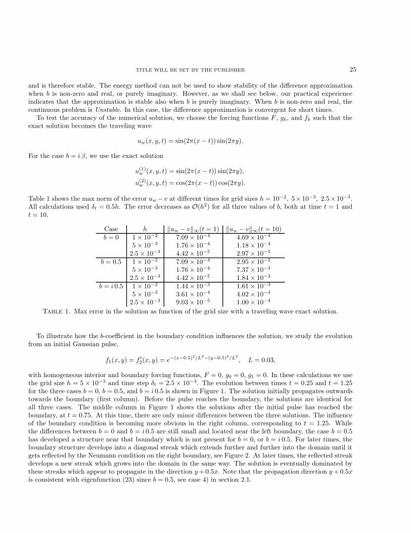
and is therefore stable. The energy method can not be used to show stability of the difference approximationwhen b is non-zero and real, or purely imaginary. However, as we shall see below, our practical experienceindicates that the approximation is stable also when b is purely imaginary. When b is non-zero and real, thecontinuous problem is Unstable. In this case, the difference approximation is convergent for short times.

To test the accuracy of the numerical solution, we choose the forcing functions F , gk, and fk such that theexact solution becomes the traveling wave

uw(x, y, t) = sin(2π(x− t)) sin(2πy).

For the case b = i β, we use the exact solution

u(1)w (x, y, t) = sin(2π(x− t)) sin(2πy),

u(2)w (x, y, t) = cos(2π(x− t)) cos(2πy).

Table 1 shows the max norm of the error uw − v at different times for grid sizes h = 10−2, 5× 10−3, 2.5× 10−3.All calculations used δt = 0.5h. The error decreases as O(h2) for all three values of b, both at time t = 1 andt = 10.

Case h ‖uw − v‖∞(t = 1) ‖uw − v‖∞(t = 10)b = 0 1× 10−2 7.09× 10−4 4.69× 10−4

5× 10−3 1.76× 10−4 1.18× 10−4

2.5× 10−3 4.42× 10−5 2.97× 10−5

b = 0.5 1× 10−2 7.09× 10−4 2.95× 10−2

5× 10−3 1.76× 10−4 7.37× 10−3

2.5× 10−3 4.42× 10−5 1.84× 10−3

b = i 0.5 1× 10−2 1.44× 10−3 1.61× 10−3

5× 10−3 3.61× 10−4 4.02× 10−4

2.5× 10−3 9.03× 10−5 1.00× 10−4

Table 1. Max error in the solution as function of the grid size with a traveling wave exact solution.

To illustrate how the b-coefficient in the boundary condition influences the solution, we study the evolutionfrom an initial Gaussian pulse,

f1(x, y) = f ′2(x, y) = e−(x−0.5)2/L2−(y−0.5)2/L2

, L = 0.03,

with homogeneous interior and boundary forcing functions, F = 0, g0 = 0, g1 = 0. In these calculations we usethe grid size h = 5 × 10−3 and time step δt = 2.5× 10−3. The evolution between times t = 0.25 and t = 1.25for the three cases b = 0, b = 0.5, and b = i 0.5 is shown in Figure 1. The solution initially propagates outwardstowards the boundary (first column). Before the pulse reaches the boundary, the solutions are identical forall three cases. The middle column in Figure 1 shows the solutions after the initial pulse has reached theboundary, at t = 0.75. At this time, there are only minor differences between the three solutions. The influenceof the boundary condition is becoming more obvious in the right column, corresponding to t = 1.25. Whilethe differences between b = 0 and b = i 0.5 are still small and located near the left boundary, the case b = 0.5has developed a structure near that boundary which is not present for b = 0, or b = i 0.5. For later times, theboundary structure develops into a diagonal streak which extends further and further into the domain until itgets reflected by the Neumann condition on the right boundary, see Figure 2. At later times, the reflected streakdevelops a new streak which grows into the domain in the same way. The solution is eventually dominated bythese streaks which appear to propagate in the direction y+0.5x. Note that the propagation direction y+0.5xis consistent with eigenfunction (23) since b = 0.5, see case 4) in section 2.1.


Figure 1. The solution at times t = 0.25 (left column), t = 0.75 (middle column), and t = 1.25(right column) for b = 0 (top row), b = 0.5 (middle row), and b = i 0.5 (bottom row). Thebottom row is showing the real part of the solution (u(1)).

It is also interesting to monitor the max norm of the solution for longer times when b = 0.5, see Figure 3. Notethat the solution grows exponentially with time, illustrating the Unstable nature of this boundary condition.Also note that the solution is slightly larger on the finer grid. This behavior agrees with the predicted exponentialgrowth proportional to |ω|t, because higher values of |ω| are captured on the finer grid. Note, however, thatthis growth is not due to numerical instabilities because the accuracy test shows second order convergence, atleast up to t = 10, see Table 1.

To more clearly see the difference between the cases b = 0 and b = i β we take F = 0, g0 = g1 = 0 and changethe initial data to trigger a surface wave,

f1(x, y) = us(x, y, 0), f ′2(x, y) = us(x, y,−δt),

where

us(x, y, t) = e−|βω0|x[

cos(

ω0(y −√

1− β2 t))

+ i sin(

ω0(y −√

1− β2 t))]

, βω0 > 0. (124)

This wave decays exponentially away from the x = 0 boundary with a harmonic oscillation in y, see Figure 4.

The surface wave propagates in the positive y-direction with a wave speed proportional to√

1− β2. As β → 0,


Figure 2. The solution of the unstable case (b = 0.5) at times t = 2.5 to t = 4.5 in incrementsof 0.25, starting in the top left sub-figure and progressing row-wise to the bottom right sub-figure, e.g. t = 2.75 is in the middle column of the top row.

2 4 6 8 10 12 14 16 18 20

100

102

104

Time

Figure 3. The max norm of the solution for 0 ≤ t ≤ 20 for the case b = 0.5, starting from aGaussian pulse. The blue dots correspond to grid size h = 10−2 and the red crosses haveh = 5× 10−3.

the surface wave decays slower and slower in the x-direction. In the limit β = 0, the amplitude of the wave is


constant in x which corresponds to one-dimensional wave propagation in the y-direction, consistent with thelimiting boundary condition ux = 0. There are no numerical difficulties in this limit.

0 0.1 0.2 0.3 0.4 0.5 0.6 0.7 0.8 0.9 10

0.1

0.2

0.3

0.4

0.5

0.6

0.7

0.8

0.9

1

Figure 4. The real part of the initial data for the surface wave with β = 0.5 and ω0 = 8π.

The case |β| → 1 is more difficult to solve numerically. Here we study 0.5 ≤ β < 1 and we use (124) as anapproximation of the exact solution (us is only exponentially small at x = 1 and does not exactly satisfy theboundary condition at that boundary). To make sure the amplitude of the surface wave is negligible at thex = 1 boundary, we choose

ω0 = 8π, e−|βω0| = e−4π ≈ 3.48× 10−6, β = 0.5.

In Table 2 we show the max norm of the error us − v for different values of β. The case β = 0.5 shows secondorder convergence, both at time t = 1 and t = 10. As can be expected in wave propagation problems, the erroris dominated by the phase error, which explains why it is about 10 times larger at t = 10 compared to t = 1.For β = 0.9, the error still converges to second order accuarcy at time t = 1, but shows an unexpected patternat time t = 10. Here the error is larger for the intermediate grid size h = 5× 10−3 than for the coarse grid sizeh = 10−2. This behavior is explained by studying the time history of the error, see Figure 5. For h = 10−2,the max error occurs at t ≈ 5.5 when the numerical solution is about 180 degrees out of phase with the exactsolution. At later times the error in the numerical solution decreases because it is between 180 and 360 degreesout of phase. The grid with h = 5× 10−3 is barely fine enough to capture the solution at time t = 10 becausethe phase error exceeds 90 degrees. As a result we don’t see the expected second order convergence when thegrid is refined to h = 2.5 × 10−3. However, the error at t = 10 is about 10 times larger than at t = 1 for thefinest grid, which indicates that this resolution is adequate for β = 0.9. The situation is even more dire forβ = 0.99. Here the errors at time t = 1 show a simular behavior as at t = 10 for β = 0.9, so only the finestgrid provides adequate resolution at t = 1. At t = 10, the error displays a completely erratic behavior with the


largest error for the finest grid. An even finer grid would be necessary to obtain an accurate solution at t = 10,when β = 0.99.

Case h ‖us − v‖∞(t = 1) ‖us − v‖∞(t = 10)β = 0.5 1× 10−2 2.44× 10−2 2.38× 10−1

5× 10−3 6.35× 10−3 6.19× 10−2

2.5× 10−3 1.60× 10−3 1.56× 10−2

β = 0.9 1× 10−2 6.04× 10−1 2.46× 10−1

5× 10−3 1.58× 10−1 1.40× 100

2.5× 10−3 4.00× 10−2 3.95× 10−1

β = 0.99 1× 10−2 1.67× 100 1.37× 100

5× 10−3 5.20× 10−1 1.81× 10−1

2.5× 10−3 1.44× 10−1 1.47× 100

Table 2. Max error in the solution as function of the grid size when the exact solution is thesurface wave us(x, y, t).

0 1 2 3 4 5 6 7 8 9 100

0.5

1

1.5

2

Figure 5. The max norm of the error as function of time for a surface wave with β = 0.9computed on a grid with h = 10−2 (blue), h = 5× 10−3 (green), and h = 2.5× 10−3 (red).

So why is it so hard to calculate an accurate numerical solution as |β| → 1? The spatial resolution in termsof grid points per wave length only depends on ω0. With ω0 = 8π, the wave length is 1/4 and grid sizesh = 10−2, 5 × 10−3, 2.5 × 10−3 correspond to 25, 50, and 100 grid points per wave length, respectively. Theexponential decay in the x-direction only depends weakly on β and never exceeds e−|ω0|x for β < 1. Hence thesolution varies on the same length scale in the x- and y-directions. Furthermore, the temporal resolution interms of time steps per period only improves as |β| → 1 because the wave speed goes to zero in this limit. Weconclude that the numerical difficulties are not due to poor resolution of the solution.

To further analyze the cause of the poor accuracy in the numerical solution for |β| → 1, we decompose theproblem (108)-(112) into two parts,

u(x, y, t) = U(x, y, t) + u′(x, y, t),

such that U satisfies a doubly periodic problem on an extended domain,

Utt = Uxx + Uyy + F (x, y, t), −1 ≤ x ≤ 2, 0 ≤ y ≤ 1, t ≥ 0,

subject to initial conditions,

U(x, y, 0) = f1(x, y), Ut(x, y, 0) = f2(x, y), −1 ≤ x ≤ 2, 0 ≤ y ≤ 1,


and periodic boundary conditions

U(x, y, t) = U(x, y + 1, t), −1 ≤ x ≤ 2, t ≥ 0,

U(x, y, t) = U(x+ 3, y, t), 0 ≤ y ≤ 1, t ≥ 0.

The interior forcing function and the initial data can be smoothly extended to become 3-periodic in the x-direction, without changing them on the original domain,

F (x, y, t) = F (x, y, t), fk(x, y) = fk(x, y), 0 ≤ x ≤ 1, 0 ≤ y ≤ 1, t ≥ 0.

The problem for U is independent of the b-coefficient in the boundary condition and can easily be solvednumerically.

The difference u′ = u − U satisfies the scalar wave equation (108)-(112) with homogeneous interior forcing,homogeneous initial data, but inhomogeneuos boundary conditions,

u′x − b u′y = g′0(y, t) x = 0, 0 ≤ y ≤ 1, t ≥ 0, (125)

u′x = g′1(y, t) x = 1, 0 ≤ y ≤ 1, t ≥ 0, (126)

The boundary forcing functions depend on U according to

g′0(y, t) = g0(y, t)− (Ux(0, y, t)− b Uy(0, y, t)) , 0 ≤ y ≤ 1, t ≥ 0,

g′1(y, t) = g1(y, t)− Ux(1, y, t), 0 ≤ y ≤ 1, t ≥ 0.

The corresponding half-plane problems were analyzed in section 2.2. The accuracy problems are unlikely toarise from the Neumann boundary condition at x = 1 since it is independent of the b-coefficient. However, thehalf-plane problem subject to (125) satisfies the estimates of Theorem 2.8. Here, b = i β corresponds to case2), and estimate (39) shows that the Laplace-Fourier transform of u′ satisfies

|u′(0, ω, s)|2 ≤ Cβ2

1− β2

|g′0|2η2

, Re s = η > 0, (127)

for (ω, s) in the vicinity of the generalized eigenvalue s0 = ±i√

1− β2 ω0. In general, the solution becomesunbounded as |β| → 1. The truncation error terms which perturb the numerical solution are therefore amplified

by a factor 1/√

1− β2, which explains the poor accuracy in the numerical solution as |β| → 1.For boundary data g0(y, t) which have a Laplace-Fourier transform that can be written as

g0(ω, s) = sG(ω, s),

estimate (127) becomes

|u′(0, ω, s)|2 ≤ Cβ2

1− β2

|s|2|G|2η2

≈ Cβ2

|s0|2/ω20

|s|2|G|2η2

= Cβ2ω20

|G|2η2

, s→ s0.

Hence the |β| → 1 singularity cancels out and the solution is bounded independently of β. The factor ‘s’ onthe Laplace transform side corresponds to a time-derivative on the un-transformed side. Hence, the solutionis bounded independently of β if the boundary forcing can be written as a time-derivative of a function withbounded Laplace-Fourier transform,

g0(y, t) = Gt(y, t), G(y, 0) = 0,

∣

∣

∣

∣

∫ 1

y=0

∫ ∞

t=0

e−2πiωye−stG(y, t) dtdy

∣

∣

∣

∣

<∞, Re s ≥ 0.


The latter condition is satisfied if G(y, t) is in L1, i.e.,

∫ 1

y=0

∫ ∞

t=0

|G(y, t)| dtdy <∞. (128)

To test this theory numerically, we use a homogeneous interior forcing (F = 0) and homogeneous initialconditions (f1 = f2 = 0), homogeneous forcing on the x = 1 boundary (g1 = 0), and consider three different

forcing functions on the x = 0 boundary: g(1)0 (y, t) = G(y, t), g

(2)0 (y, t) = Gt(y, t), and g

(3)0 (y, t) = Gtt(y, t).

Here we choose G(y, t) to trigger a surface wave:

G(y, t) = us(0, y, t) e−(t/t0−7)2 , t0 = 0.2,

where us is defined by (124). The Gaussian pulse exp(−(t/t0 − 7)2) decays exponentially fast away from itscenter at t = 7t0. For example, it equals 1.23× 10−4 at t = 7t0 ± 3t0, and 5.24× 10−22 at t = 7t0 ± 7t0. The

function G(y, t) satisfies (128), so our theory predicts that boundary forcings g(2)0 and g

(3)0 should give solutions

that are bounded independently of β. However, the time-integral of a Gaussian pulse is the error-function (erf),

so the boundary forcing g(1)0 does not satisfy (128).

In the numerical calculations we take ω0 = 8π and study the cases β = 0.5, β = 0.9, and β = 0.99. The gridsize and time step are h = 2.5× 10−3 and δt = 0.5h. The max norm of the solution as function of time is shown

in Figure 6. The case g(1)0 = G in the top sub-figure illustrates the general case where the solution grows as

|β| → 1. Note that estimate (127) predicts the solution to grow like β/√

1− β2, which means that the solutionshould be about 3.5 times larger for β = 0.99 than β = 0.9. In the numerical calculation, the max norm of thesolution grows from about 0.75 for β = 0.9 to 3.75 for β = 0.99, which is slightly faster than predicted by theory.

The case g(3)0 = Gtt in the bottom sub-figure shows the opposite situation when the solution decays as β → 1

because the forcing function is a second time-derivative of a function with bounded L1 norm, corresponding to

an s2 factor on the Laplace transform side. The intermediate case g(2)0 = Gt is shown in the middle sub-figure.

Here the solution grows between β = 0.9 and β = 0.99, but not as fast as for g(1)0 . To more closely study the

behavior near β = 1, we take β = 0.995, 0.999 and 0.9997 corresponding to√

1− β2 ≈ 0.0998, 0.0447 and0.0244, respectively. To properly resolve the solution we here use an extra fine grid with h = 1.25× 10−3 andδt = 0.5h. The max norm of the solutions, shown in Figure 7, reveal that the solution indeed stays bounded

independently of β, confirming our theory also for boundary forcing g(2)0 = Gt.

Appendix

In this appendix we collect a number of auxilary lemmas.

Lemma A.1. The solution of

yx = λy + F, Re λ > 0, 0 ≤ x <∞ (129)

satisfies the estimate

|y(0)|2 ≤ 1

2Re λ‖F‖2, ‖y‖2 ≤ 1

(Re λ)2‖F‖2, ‖F‖2 =

∫ ∞

0

|F |2dx.

Proof. Integration by parts gives us

(y, yx) = −|y(0)|2 − (yx, y), i.e., 2Re(y, yx) = −|y(0)|2.


0 1 2 3 4 5 6 7 8 9 100

1

2

3

4

0 1 2 3 4 5 6 7 8 9 100

5

10

15

0 1 2 3 4 5 6 7 8 9 100

50

100

150

Figure 6. The max norm of the solution as function of time for the boundary forcing functions

g(1)0 = G (top), g

(2)0 = Gt (middle), and g

(3)0 = Gtt (bottom). In each figure, the green, blue,

and red curves correspond to β = 0.5, β = 0.9, and β = 0.99, respectively.

Therefore

1

2|y(0)|2 +Re λ ‖y‖2 = −Re (y, F ) ≤ ‖y‖ ‖F‖

≤ α

2Re λ ‖y‖2 + 1

2α

‖F‖2Re λ

, α > 0.

With α = 2 the first inequality follows. With α = 1 the second inequality follows.

Lemma A.2. The solution of

yx = −λy + F, y(0) = g, Re λ > 0, 0 ≤ x <∞,

satisfies

‖y‖2 ≤ 1

Reλ|g|2 + 1

(Reλ)2‖F‖2. (130)


0 1 2 3 4 5 6 7 8 9 100

2

4

6

8

10

12

14

16

18

Time

Figure 7. The max norm of the solution as function of time for the boundary forcing function

g(2)0 = Gt for β = 0.995 (blue/dots), β = 0.999 (red/diamonds) and β = 0.9997 (black/plusses).

Proof.〈y, y〉x = 2Re 〈y, yx〉 = −2(Reλ)|y|2 + 2Re 〈y, F 〉.

As y ∈ L2, integrating we have

−|y(0)|2 = −2Reλ ‖y‖2 + 2Re (y, F )

≤ −2Reλ ‖y‖2 + 2 ‖y‖ ‖F‖

≤ −2Reλ ‖y‖2 +Reλ ‖y‖2 + ‖F‖2Reλ

.

Thus,

Reλ ‖y‖2 ≤ |y(0)|2 + ‖F‖2Reλ

and the lemma follows.

Lemma A.3. Let a, b be real and consider√a+ ib with −π < arg(a + ib) ≤ π, arg

√z = 1

2arg z. Then, thefollowing inequalities hold

2−1/4√

|a|+ |b| ≤ |√a+ ib| ≤

√

|a|+ |b| (131)

2−3/4|√a+ ib| ≤ 2−3/4

√

|a|+ |b| ≤ Re√a+ ib ≤ |

√a+ ib| for a ≥ 0, (132)

2−5/4 |b||√a+ ib|

≤ 2−1 |b|√

|a|+ |b|≤ Re

√a+ ib ≤ |

√a+ ib| for a ≤ 0. (133)

Proof. In polar notation a+ ib = ρeiθ, ρ =√a2 + b2 > 0, −π < θ ≤ π, and

√a+ ib =

√ρ ei

θ2

We have√

|a|+ |b| = √ρ√

| cos θ|+ | sin θ| ≥ 21/4√ρ

and the first inequality in (131) follows. The second inequality in (131) follows from the triangle inequality. Ifa ≥ 0 then θ

2 ∈ [−π/4, π/4] and (131) implies

|√a+ ib| ≥ Re

√a+ ib =

√ρ cos(θ/2) ≥

√2

2ρ ≥ 2−3/4

√

|a|+ |b| ≥ 2−3/4|√a+ ib|


which is (132). To prove (133) notice that, as a ≤ 0,

|b|√

|a|+ |b|≤ |b|

|√a+ ib|

=ρ sin θ√

ρ=

√ρ 2 sin(θ/2) cos(θ/2) ≤ 2Re

√a+ ib

therefore1

2

|b|√

|a|+ |b|≤ Re

√a+ ib ≤ |

√a+ ib|

and the inequality follows from (131).

For the forthcoming lemmata, we remind the reader that s = η+ iξ, where η, ξ ∈ R, and κ =√ω2 + s2. We

shall now apply the last lemma to

κ =√

ω2 + η2 − ξ2 + 2iξη, i.e., a = ω2 + η2 − ξ2, b = 2ξη.

In the following three lemmas we denote by δ a constant with 0 < δ < 1.

Lemma A.4. Letδ1 = 2−1/4

√δ, δ2 = 21/2(1− δ)1/4, δ3 = min(δ1, δ2).

Then

|κ| ≥

δ1√

ω2 + |s|2 if |ω2 + η2 − ξ2| ≥ δ(ω2 + |s|2)δ2

√

√

|s|2 + ω2 η otherwise.(134)

Also, always|κ| ≥ δ3η. (135)

Proof. By (131) we obtain, for the first case,

|κ| ≥ 2−1/4√

|ω2 + η2 − ξ2|+ 2|ξ|η ≥ 2−1/4√δ√

ω2 + |s|2.

If |ω2 + η2 − ξ2| < δ(ω2 + |s|2), then

2ξ2 ≥ (1− δ)(ω2 + ξ2 + η2) = (1 − δ)(ω2 + |s|2).

Therefore

|κ| ≥ 2−1/4√

2|ξ|η ≥√

2√1− δ

√

ω2 + |s|2 η.Also

√

ω2 + |s|2 ≥ η implies (135). This proves the lemma.

Lemma A.5.

Reκ ≥

2−5/4|κ| if ω2 + η2 − ξ2 ≥ 0,

2−3/4

√ω2+|s|2|κ| η if ω2 + η2 − ξ2 < 0.

Reκ ≥ δ4η, δ4 = 2−3/4min(1, δ3).

Proof. If ω2 + η2 − ξ2 ≥ 0, then (132) gives us

Reκ ≥ 2−3/4|κ| ≥ 2−3/4δ3η.

If ω2 + η2 − ξ2 < 0, then 2ξ2 ≥ ω2 + η2 + ξ2 = ω2 + |s|2. Therefore (133) gives us

Reκ ≥ 2−5/4 2|ξ|η|κ| ≥ 2−3/4

√

ω2 + |s|2|κ| η ≥ 2−3/4η.



Lemma A.6.

|κ|Reκ ≥ δ6√

ω2 + |s|2 η, δ6 = min(

δ1δ4, 2−5/4δ22 , 2

−3/4)

.

Proof. If ω2 + η2 − ξ2 ≥ 0, and |ω2 + η2 − ξ2| ≥ δ(ω2 + |s|2), then (134) and (136) give us

|κ|Reκ ≥ δ1√

ω2 + |s|2 δ4η.

If ω2 + η2 − ξ2 ≥ 0, and |ω2 + η2 − ξ2| < δ(ω2 + |s|2), then (134) and (136) give us

|κ|Reκ ≥ 2−5/4|κ|2 ≥ 2−5/4δ22√

ω2 + |s|2 η.

Finally, if ω2 + η2 − ξ2 < 0, by (136) we obtain

|κ|Reκ ≥ 2−3/4√

|ω|2 + |s|2 η.


Lemma A.7. Assume that, for the boundary condition 1), a > 0, |b| < 1. Then there is a constant δ > 0 suchthat, for all ω and s with Re s ≥ 0,

|s+ aκ− ibω| ≥ δ√

|s|2 + |ω|2.For the proof, see Lemma 3 of [4].Finally we have a lemma similar to Lemma A.4 and Lemma A.6 but for the normalized variables

κ′ =√

η′2 − ξ′2 + ω′2 + 2iξ′ω′, ξ′2 + ω′2 = 1, |η′| ≪ 1.

By Lemma A.3,

|κ′| ≥ 2−1/4√

| − ξ′2 + ω′2 + η′2|+ 2|ξ′| |η′|Reκ′ ≥ 2−3/4

√

| − ξ′2 + ω′2 + η′2|+ 2|ξ′| |η′| if ξ′2 ≤ ω′2 + η′2,

Reκ′ ≥ |ξ′|η′√

| − ξ′2 + ω′2 + η′2|+ 2|ξ′| |η′|if ξ′2 > ω′2 + η′2.

(136)

Lemma A.8. There is a constants δ > 0 such that

|Reκ′| ≥ δη′, |κ′| ≥ 2−1/4 η′, |κ′| |Reκ′| ≥ δ6 η′.

where δ6 is that of Lemma A.6.

Proof. From Lemma Lemma A.6, dividing by ω2 + ξ2,

|κ′| |Reκ′| =|κ| Reκω2 + ξ2

≥ δ6

√

ω2 + |s|2√

ω2 + ξ2η

√

ω2 + ξ2≥ δ6 η

′.

Now if ω′2 − ξ′2 ≥ 0, then ω′2 − ξ′2 + η′2 ≥ η′2, and

√

|ω′2 − ξ′2 + η′2|+ 2|ξ′|η′ ≥√

η′2 + 2|ξ′|η′ ≥ η′,

so that, by Lemma A.3,|κ′| ≥ 2−1/4η′, and Reκ′ ≥ 2−3/4η′.


If ω′2 − ξ′2 ≤ 0 then |ξ′2| ≥ 1/2. From (136)

|κ′| ≥ 2−1/4

√

2√2 η′ ≥ 21/2 η′.

This last estimate also holds for |Reκ′| when ω′2 − ξ′2 + η′2 ≥ 0. When ω′2 − ξ′2 + η′2 ≤ 0 we just use|ω′2 − ξ′2 + η′2| + 2|ξ′| η′ ≤ const. and from (136) the estimate for Reκ′ follows from (136). This proves thelemma.

We thank Prof. Oscar Reula who participated in the original discussions leading to this work.

References

[1] H.-O. Kreiss. Initial boundary value problems for hyperbolic systems. Commun. Pur. Appl. Math., 23:277–298, 1970.[2] H.-O. Kreiss and J. Lorenz. Initial-boundary value problems and the Navier-Stokes equations. Academic Press, San Diego, 1989.[3] B. Gustafsson, H.-O. Kreiss and J. Oliger. Time dependent problems and difference methods. Wiley-Interscience, 1995.[4] H.-O. Kreiss and J. Winicour. Problems which are well posed in a generalized sense with applications to the Einstein equations.

Class. Quantum Grav., 23(16):405–420, 2006.[5] M. S. Agranovich. Theorem on matrices depending on parameters and its applications to hyperbolic systems. Funct. Anal.

Appl., 6:85–93, 1972.

initial-boundary value problems for … · of partial differential equations ... initial-boundary...

Documents