Bathtub Dynamics:Initial Results of a Systems Thinking Inventory

SWP#4 132

Linda Booth SweeneyHarvard University Graduate School of Education

Linda_Booth_Sweeney harvard.edu

John D. StermanMIT Sloan School of Management

Jstermanmit.edu

Version 1.2, September 2000Presented at the 2000 International System Dynamics Conference,

Bergen, Norway

Financial support for this project was provided by the MIT Sloan School of ManagementOrganizational Learning Fund. Nelson Repenning graciously permitted us to administer the tasks inhis introductory system dynamics class. We also thank Jim Doyle, Michael Radzicki, Terry Tivnanthe referees for helpful comments. Christopher Hunter assisted with data entry.

Bathtub Dynamics:

Initial Results of a Systems Thinking Inventory

Linda Booth SweeneyJohn Sterman

ABSTRACT

In a world of accelerating change, educators, business leaders, environmentalists and scholars are

calling for the development of systems thinking to improve our ability to take effective actions.

Through courses in the K-12 grades, universities, business schools, and corporations, advocates

seek to teach people to think systemically. These courses range from one-day workshops with no

mathematics to graduate level courses stressing formal modeling. But how do people learn to think

systemically? What type of skills are required? Does a particular type of academic background

improve one's ability to think systemically? What systems concepts are most readily understood?

Which tend to be most difficult to grasp? We describe initial results from an assessment tool or

systems thinking inventory. The inventory consists of brief tasks designed to assess particular

systems thinking concepts such as feedback, delays, ird stocks and flows. Initial findings

indicate that subjects from an elite business school with essentially no prior exposure to system

dynamics concepts have a poor level of understanding of stock and flow relationships and time

delays. Performance did not vary systematically with prior education, age, national origin, or

other demographic variables. We hope the inventory will eventually provide a means for testing

the effectiveness of training and decision aids used to improve systems thinking skills. We discuss

the implications of these initial results and explore steps for future research.

1

1 INTRODUCTION

The use of systems thinking and system dynamics is increasing dramatically, yet there is little

evidence, or even systematic research, to support educators' and consultants' faith in its efficacy.

Partisans of systems thinking and systems dynamics education are convinced that such instruction

produces or facilitates important thinking skills. Students are promised to learn "how to better

identify issues, make better decisions and to gain knowledge and insight they can share with others

in their organization" (Microworlds Inc. Brochure, 1997). Students are also said to learn "how to

get to the roots causes of problematic situations and issues at work within an organization... and to

have better creative problem solving skills" (TLC Team Learning Lab brochure, 1998). It is also

claimed that with systems thinking skills, "people start seeing and dealing with interdependencies

and deeper causes of problems" (Senge, et al. 1999).

Unfortunately, claims that systems thinking interventions can produce beneficial changes in

thinking, behavior, or organizational performance have outstripped evaluative research testing

these claims. Existing studies include Bakken et al.'s (1992) study of learning from management

flight simulators at a high tech firm; Zulauf's (1995) study of systems thinking and cognition;

Cavaleri and Sterman's (1995) evaluation of an intervention in the insurance industry; Vennix's

(1996) work on the impact of computer-based learning environments on policy making; Mandinach

and Cline's (1994) assessment of a systems thinking project in the K-12 arena; see also Doyle,

Radzicki and Trees (1996, 1998), Ossimitz (1996), Boutilier (1981), Chandler and Boutilier

(1992), Dangerfield and Roberts (1995), and the special issue of the System Dynamics Review on

systems thinking in education (Gould 1993). Despite these studies, however, there is little

consensus, and major questions about people's native systems thinking abilities and the efficacy of

interventions designed to develop these capacities remain unanswered.

Moreover, there are as many lists of systems thinking skills as there are schools of systems

thinking. Each stresses different concepts, from the ability to deduce behavior patterns and see

circular cause-effect relations (Richmond 1993), to the use of "synthesis" to reveal a system's

2

structure (Ackoff and Gharajedaghi 1984), to the view of systems thinking as a discipline of

organizational learning for "seeing wholes." (Senge 1990).

Most systems thinking advocates agree that much of the art of systems thinking involves the ability

to represent and assess dynamic complexity (e.g., behavior that arises from the interaction of a

system's agents over time), both textually and graphically. Specific systems thinking skills include

the ability to:

* understand how behavior of the system arises from the interaction of its agents over time(i.e., dynamic complexity);

* discover and represent feedback processes (both positive and negative) hypothesized tounderlie observed patterns of system behavior;

* identify stock and flow relationships;

* recognize delays and understand their impact;

* identify nonlinearities;

* recognize and challenge the boundaries of mental (and formal) models.

Underlying these systems thinking abilities are more basic skills which are taught as part of most

high school curricula:

· interpreting graphs, creating graphs from data;

· telling a story from a graph, creating a graph of-behavior over time from a story;

· identifying units of measure (i.e. Federal Deficit = $/time period);

· basic understanding of probability, logic and algebra.

Effective systems thinking also requires good scientific reasoning skills such as the ability to use a

wide range of qualitative and quantitative data, and familiarity with domain-specific knowledge of

the systems under study. For example, systems thinking studies of business issues requires some

knowledge of psychology, decision making, organizational behavior, economics, and so on.

The challenge facing educators is not only to develop ways to teach these skills, but also to

measure the impact of such courses on students' ability to think dynamically and systemically.

Doing so requires instruments to assess students' systems thinking abilities prior to and after

exposure to the concepts. In this paper we take first steps toward the development of an inventory

of test items that measure people's performance on specific systems thinking concepts. We

develop and test items focusing on some of the most basic systems thinking concepts: stocks and

flows, time delays, and negative feedback. Additional items under development will address other

dimensions of systems thinking.

In this paper we use the inventory to assess understanding of basic systems concepts in subjects

with little prior exposure to systems thinking. The subject pool, students at the MIT Sloan School

of Management, are highly educated and possess unusually strong background in mathematics and

the sciences compared to the public at large. If their ability to understand such basic concepts as

stocks and flows and time delays is poor, the performance of the general public is not likely to be

better. As we show, the performance of these students was quite poor, and the students exhibited

persistent, systematic errors in their understanding of these basic building blocks of complex

systems. Broad prevalence of such deficits poses significant challenges to educators and

organizations seeking to develop systems thinking or formal models to address pressing issues.

A number of experimental studies examine how people perform in dynamically complex

environments. These generally show that performance deteriorates rapidly (relative to optimal)

when even modest levels of dynamic complexity are introduced, and that learning is weak and

slow even with repeated trials, unlimited time, and performance incentives (e.g., Sterman 1989a,

1989b, Paich and Sterman 1993, Diehl and Sterman 1995. See also Brehmer 1992, Frensch and

Funke 1995, and D6rner 1980, 1996). The usual explanation for our poor performance in these

studies is bounded rationality: the complexity of the systems we are called upon to manage

overwhelms our cognitive capabilities. Implicit in this account is the assumption that while we are

unable to correctly infer how a complex system consisting of many interacting elements and agents

will behave or how it should be managed, we do understand the individual building blocks such as

stocks and flows and time delays. Our results challenge this view, suggesting the problems people

have with dynamics are more basic and, perhaps, more difficult to overcome.

4

2 METHOD

We created several tests to explore students' baseline systems thinking abilities. Each test

consisted of a few paragraphs posing a problem. 'Participants were asked to respond by drawing a

graph of the expected behavior over time. The items were designed to be simple, and can be

answered without use of mathematics beyond high school (primarily simple arithmetic).

A. Stocks and Flows: The Bath Tub/Cash Flow (BT/CF) Task

Stocks and flows are fundamental to the dynamics of systems (Forrester 1961). Stock and flow

stuctures are pervasive in systems of all types, and the stock/flow concept is central in disciplines

ranging from accounting to epidemiology. The BT/CF task tests subjects' understanding of stock

and flow relationships by asking them to determine how the quantity in a stock varies over time

given the rates of flow into and out of the stock. This ability, known as graphical integration, is

basic to understanding the dynamics of complex systems.

To make the task as concrete as possible we used two cover stories: The Bath Tub (BT) condition

described a bathtub with water flowing in and draining out (Figure 1); the Cash Flow (CF)

condition described cash deposited into and withdrawn from a firm's bank account (Figure 2).

Both cover stories describe everyday contexts quite familiar to the subjects. Students are prompted

to draw the time path for the quantity in the stock (the contents of the bathtub or the cash account).

Note the extreme simplicity of the task. There are no feedback processes-the flows are

exogenous. Round numbers are used so it is easy to calculate the net flow and quantity added to

the stock. The form provides a blank graph for the stock on which subjects can draw their answer.

Note also that the numerical values of the rates and initial stock are the same in the BT and CF

versions (the only difference is the time unit: seconds for the BT case; weeks for the CF case).'

'We tested two versions of BT/CF task 1. One (shown in Figures 1 and 2) included the scale and units of measurefor the stock. The second omitted the units and scale; subjects had to specify their own scale. There were nosignificant differences in performance between the scale/no scale conditions (the hypothesis that the means for theunits and no units conditions were equal could not be rejected at p 0.86), so we dropped this treatment in BT/CFtask 2.

We also tested two different patterns for the flows, a square wave pattern (task 1) and a sawtooth

pattern (task 2). Figure 1 shows the square wave; Figure 2 shows the sawtooth. We tested all

four combinations of cover story (BT/CF) and inflow pattern (task /task 2). In the square wave

pattern used in task 1 both inflow and outflow are constant during each segment. This is among

the simplest possible graphical integration task-if the net flow into a stock is a constant, the stock

increases linearly. The different segments are symmetrical, so solving the first (or, at most, first

two) segments gives the solution to the remaining segments. We expected that performance on this

task would be extremely good, so we also tested performance for the case where the inflow is

varying: In BT/CF task 2 the outflow is again constant and the inflow follows a sawtooth wave,

rising and falling linearly. Task 2, though still elementary, provides a slightly more difficult test of

the subjects' understanding of accumulations, in particular, their ability to relate the net rate of flow

into a stock to the slope of the stock trajectory.

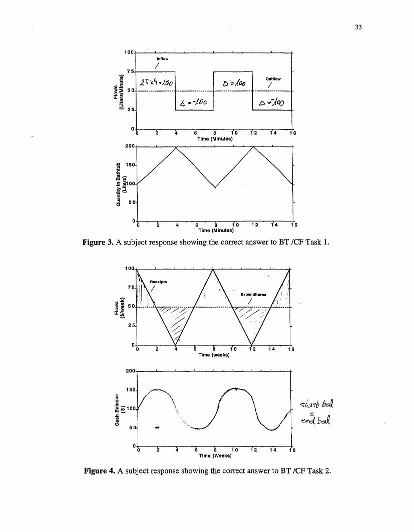
Solution to Task 1: The correct answer to BT/CF task 1 is shown in Figure 3 (this is an actual

subject response). Note the following features:

1. When the inflow exceeds the outflow, the stock is rising.

2. When the outflow exceeds the inflow, the stock is falling.

3. The peaks and troughs of the stock occur when the net flow crosses zero (e.g., at t = 4, 8,12, 16).

4. The stock should not show any discontinuous jumps (it is continuous).

5.- During each segment the net flow is constant so the stock must be rising (falling) linearly.

6. The slope of the stock during each segment is the net rate (e.g., ±25 units/time period).

7. The quantity added to (removed from) the stock during each segment is the area enclosedby the net rate (e.g., 25 units/time period * 4 time periods = 100 units, so the stock peaksat 200 units and falls to a minimum of 100 units).

The first five items describe qualitative features of the behavior and do not require even the most

rudimentary arithmetic. Indeed, the first three are always true for any stock with any pattern of

flows; they are fundamental to the concept of accumulation. The last two describe the behavior of

the stock quantitatively, but the arithmetic required to answer them is trivial. Solving the problem

is straightforward (the description below assumes the BT cover story). First, note that the

behavior divides into distinct segments in which the inflow is constant (the outflow is always

6

constant). During segment 1 (0 < t < 4) the net inflow is 75 - 50 = 25 liters/second (l/s). Next

calculate the total added to the stock by the end of the segment, given by the area bounded by the

net rate curve between 0 < t < 4 s: 25 1/s * 4 s = 100 liters. Finally, since the net flow is constant

during the segment the stock rises at a constant rate: draw a straight line between the initial stock at

100 liters and the stock at the end of the segment at 200 liters. The slope of this line is 100/4 = 25

1/s. Proceeding to segment 2 (4 < t < 8), the inflow drops to 50 1/s so the net flow is -25 1/s. The

net flow is the same as in segment 1 but with opposite sign, so the stock loses the same quantity

between time four and time eight as it gained between time zero and four. If the subject does not

notice the symmetry, the same procedure used in segment 1 can be used to determine that the stock

loses 100 1 by t = 8. Subsequent segments simply repeat the pattern of the first two.

Solution to Task 2: Figure 4 shows the correct solution to task 2 (again, an actual subject

response). The solution must have the following features, which we used to code subject

responses and assign a score.

1. When the inflow exceeds the outflow, the stock is rising.

2. When the outflow exceeds the inflow, the stock is falling.

3. The peaks and troughs of the stock occur when the net flow crosses zero (i.e., at t = 2, 6,10, 14).

4. The stock should not show any discontinuous jumps (it is continuous).

5. The slope of the stock at any time is the net rate. Therefore

a. When the net flow is positive and falling, the stock is rising at a diminishing rate (0 < t< 2;8 <t< 10).

b. When the net flow is negative and falling, the stock is falling at an increasing rate (2 < t<4; 10<t< 12).

c. When the net flow is negative and rising, the stock is falling at a decreasing rate (4 < t <6; 12 < t < 14).

d. When the net flow is positive and rising, the stock is rising at an increasing rate (6 < t <8; 14 < t < 16).

6. The slope of the stock when the net rate is at its maximum is 50 units/period (t = 0, 8, 16).

7. The slope of the stock when the net rate is at its minimum is -50 units/period (t = 4, 12).

8. The quantity added to (removed from) the stock during each segment of 2 periods is thearea enclosed by the net rate (e.g., a triangle with area ±(1/2) * 50 units/period * 2 periods= +50 units). The stock therefore peaks at 150 units and reaches a minimum of 50 units.

7

As in task 1, the first five items describe qualitative features of the behavior and do not require

even the most rudimentary arithmetic. The last three describe the behavior of the stock

quantitatively, but the arithmetic required is trivial.

Answering the question also requires subjects to read and interpret the graph of the rates, and to

add points to an existing graph (the level of the stock at various points in time). For task 2,

subjects must also know the formula for the area of a triangle (for §7) and be able to construct a

straight line with slope ±50 units/time period to show the slope of the stock properly at the

inflection points t = 0, 4, 8, 12, and 16 (for §6).2

B. The Impact of Time Delays: The Manufacturing Case

The BT/CF tasks address subjects' understanding of the basic concepts of accumulation, without

any feedbacks or time delays. However, feedback processes and time delays are pervasive in

complex systems and often have a significant effect on their dynamics. Time delays can cause

instability and oscillation, especially when embedded in negative feedback loops. The

Manufacturing Case (MC) assesses students' understanding of stock and flow relationships in the

presence of a time delay and a single negative feedback loop. The MC task also tests their ability to

create a graph that tells a story about a particular behavior over time, and to draw inferences about

the dynamics of a system from a description of its structure (Figure 5).

The manufacturing case is an example of a simple stock management task (Sterman 1989a,

1989b). The stock management task is a fundamental structure in many systems and at many

levels of analysis, from filling a glass of water to regulating your alcohol consumption to inventory

control and capital investment (see Sterman 2000, ch. 17 for discussion and examples). In the

stock management task, the system manager seeks to maintain a stock at a target or desired level in

the face of disturbances such as losses or usage by regulating the inflow to the stock. Often there

2 Any subject who recalls elementary calculus knows that the trajectory of the stock follows a parabola within eachsegment. However, we did not require subjects to recognize or indicate this in their responses. They received fullmarks as long as they showed the slope for the stock changing in the proper fashion as indicated in §5, whether itwas parabolic or not.

8

is a delay between the initiation of a control action and its effect. Here the firm seeks to control its

inventory in the face of variable customer demand and a lag between a change in the production

schedule and the actual production rate. The task involves a simple negative feedback regulating

the stock (boosting the inflow to the stock when the stock is less than desired, and cutting it when

there is a surplus).

Solution to the Manufacturing Case: Unlike the BT/CF tasks, there is no unique correct

answer to the MC task. However, the trajectories of production and inventory must follow certain

constraints, and their shapes can be determined without any quantitative analysis. The

unanticipated step increase in customer orders and production adjustment delay mean shipments

increase while production remains, for a time, constant at the original rate. Inventory therefore

declines. The firm must not only boost output to the new rate of orders, but also rebuild its

inventory to the desired level. Production must therefore overshoot orders and remain above

shipments until inventory reaches the desired level, at which point production can drop back to

equilibrium at the customer order rate.

Furthermore, since the task specifies that the desired iyentory level is constant, the area bounded

by the production overshoot must equal the quantity of inventory lost during the period when

orders exceed production, which in turn is the area between orders and production (e.g., between

week 5 and the point where production rises to the order rate). Figure 6 illustrates.

It is possible that production and inventory could fluctuate around their equilibrium values, but

while such fluctuation is not inevitable, the overshoot of production is: the only way inventory can

rise is for production to exceed orders, in exactly the same way that the only way the level of water

in a bathtub can rise is for the flow in from the tap to exceed the flow out through the drain.

A few modest assumptions allow the trajectories of production and inventory to be completely

specified. When customer orders increase from 10,000 to 11,000 widgets/week, production

remains constant at the initial rate, due to the four week lag. Inventory, therefore, begins to decline

9

at the rate of 1,000 widgets/week. What happens next depends on the distribution of the

production lag. The simplest case, and the case most subjects assumed, is to assume a pipeline

delay, that is,3

Production(t) = Desired Production(t - 4).

Assuming production follows desired production with a four week delay means production

continues at 10,000 widgets/week until week 9. During this time, inventory drops by a total of

1,000 widgets/week * 4 weeks = 4,000 widgets, thus falling to 46,000 widgets. Assuming

further that the firm understands the delay and realizes that production will remain at its original

level for four weeks, management will raise desired production above orders at week 5, keep it

above orders until an additional 4,000 widgets are scheduled for production, and then bring

desired production back down to orders. Production then traces this pattern four weeks later.

Assuming finally that production remains constant during the period of overshoot gives production

trajectories such as those shown in Figures 6 and 7. Figure 6, typical of many correct responses,

shows production rising in week 9 to 12,000 widgets/week and remaining there for the next four

weeks, giving a rectangle equal in shape to that for the period 5 < t < 9 when shipments exceed

production. Of course, the production overshoot can have any shape as long as the area equals

4,000 widgets. Figure 7 shows another correct response in which the subject shows production

rising in week 9 to 13,000 widgets/week and remaining there for two weeks. This response

clearly shows the subject understood the task well, particularly the area concept. Very few

subjects (< 0.02%) drew a pattern with the duration of the overshoot : 4 weeks while also

maintaining the correct area relationship.

In the basic version of the task subjects were asked only to sketch the trajectory of production.

Doing so requires them to infer correctly the behavior of the firm's inventory. Without a graph of

inventory this might be more difficult for subjects, making it difficult for them to correctly trace the

3 We did not penalize subjects if they selected other patterns for the delay (such as some adjustment before week 9and some after, as would be generated by a finite-order material delay, as long as production did not begin to increaseuntil after the step increase in orders.

10

production overshoot. To test this hypothesis we defined an inventory graph treatment with two

conditions. In the Inventory graph (I) condition, the page with the MC task included a blank graph

for the firm's inventory and subjects were asked to provide trajectories for both production and

inventory (as shown in Figure 5). In the No Inventory graph (-I) condition, subjects were

provided only with the graph showing customer orders and were not asked to sketch the trajectory

of inventory.4

In the -I condition performance was assessed by coding for the following criteria:

1. Production must start in equilibrium with orders.

2. Production must be constant prior to time 5 and indicate a lag of four weeks in the responseto the step increase in orders.

3. Production must overshoot orders to replenish the inventory lost during the initial periodwhen orders exceed production. Production should return to (or fluctuate around) theequilibrium rate of 11,000 widgets/week (to keep inventory at or fluctuating around thedesired level).

4. Conservation of material: The area enclosed by production and orders during the overshootof production (when production > orders) must equal the area enclosed by orders lessproduction (when production < orders).

Points 1 and 2 follow directly from the instructions, which specify that the system starts in

equilibrium, that there is a four week production lag, 4nd that the change in orders is unanticipated.

Point 3 results from the firm's policy of adjusting production to correct any inventory imbalance

and reflects the basic physics of stocks and flows, specifically that a stock falls when outflow

exceeds inflow and rises when inflow exceeds outflow. Point 4 tests conservation of material:

4 We also hypothesized that some subjects might not appreciate the negative feedback loop through which the firmcontrols inventory. To further direct attention to the inventory control process, we created a "feedback hint"treatment with two levels: in the Feedback hint (H) condition, the task description included this sentence:

"Because customer orders are quite variable, the firm strives to maintain an inventory of 50,000 units toprovide excellent customer service (that is, to be able to fill essentially 100% of every order), and theyadjust production schedules to close any gap between the desired and actual level."

In the No Hint (-H) condition the phrase "and they adjust production schedules to close any gap between the desiredand actual level" was omitted. In the first administration of the MC task all four combinations of the inventorygraph and feedback hint treatments were given. Performance on the two hint conditions was almost identical (H =0.426; -H = 0.435; the hypothesis that these means are equal cannot be rejected at p 0.86) so in the secondadministration of the MC task all subjects received the H condition, and we pooled all responses in the analysis.

11

since desired inventory is constant the quantity added to inventory during the production overshoot

just replaces the quantity lost during the initial response when orders exceed production.

Responses to the inventory graph condition were also coded for the following:

5. Inventory must initially decline (because production < orders).

6. Inventory must recover after dropping initially.

7. Inventory must be consistent with the trajectory of production and orders, i.e.,if orders > production, inventory must be falling;if orders < production, inventory must be rising;if orders = production, inventory reaches a maximum or minimum;when the difference between production and orders is a maximum the inventory

trajectory is at an inflection point (steepest absolute value of the slope)

Point 5 follows from points 1 and 2: when orders increase, production must remain at the initial

rate due to the adjustment delay. Until production increases, orders exceed output so inventory

must fall. Inventory should then rebound because the firm seeks to adjust inventory to its desired

value (point 6). Point 7 tests the consistency of the production and inventory trajectories, and

indicates whether subjects understand that the slope of a stock at any point is its net rate. Note that

point 7 does not require the production trajectory to be correct, only that the trajectory of inventory

be consistent with the production path drawn by the subject, whatever it may be.

3 SUBJECTS AND PROCEDURE

We administered the tasks above to two groups of students at the MIT Sloan School of

Management enrolled in the introductory system dynamics course. The first group received a

background information sheet, the manufacturing case, and the "paper fold" case on the first day of

class.5 Two weeks later, the same class received the bath tub cash/flow case. 6 On the first day of

the next semester a new set of students received the background information sheet and bathtub/cash

flow task 2. Students were given approximately 10 minutes in each session. They were told that

5 The Paper Fold task is described in Sterman (2000), ch. 8, and tests understanding of positive feedback andexponential growth. We will report the results of this task in another paper.6 Between the first and second rounds students covered the system dynamics perspective, the concept of feedback, andcausal loop diagrams; stocks and flows were introduced after they did the BT/CF task. Since the class is an electiveand there is some enrollment churn in the first weeks, not all those in session 1 were present for session 2, and vice-versa.

12

the purpose of the questions was to illustrate important systems thinking concepts they were about

to study and to develop a tool to assess systems thinking skills. Students were not paid or graded.

To explore whether performance on the tasks varied with educational background or other

demographic factors, we asked the subjects to fill out a background data sheet. We requested

information on their academic background, current degree program, whether English was their first

language, their country of origin, and whether they had previously played the beer distribution

game (Sterman 1989b, Senge 1990). To protect student privacy, ID codes were assigned and used

instead of names in coding and analysis. Table 1 summarizes the subject demographics.

The two groups were quite similar. They were largely comprised of male MBA students but also

included students in other master's degree programs, Ph.D. students, undergraduates, and

students cross-registered from graduate programs at other local universities, primarily Harvard.

More than half had undergraduate backgrounds in engineering, computer science, mathematics, or

the sciences, with most of the rest having business or a social science (primarily economics) as

their undergraduate field of study. Fewer than 5% had degrees in the humanities. The students are

highly international, with 35 countries represented. I group 1 English was a first language for

about 44%; in group 2 these proportions were roughly reversed. Prior to taking the test, more than

half the subjects had played the beer game as part of Sloan's MBA orientation program. These

demographics are typical of the Sloan School's student body.

Initial coding criteria were developed, then tested on a subsample of results. The coding criteria

were revised to resolve ambiguities; the final coding criteria are described above. Correct

responses to each criterion were assigned 1, and incorrect responses were given zero.

4 RESULTS

Table 2 summarizes overall performance. In general, performance is poor.

Bath Tub/Cash Flow, Task 1: Average performance on this simplest graphical integration

task was 77%. Table 3 breaks performance down by the individual coding criteria and cover

13

story. Subjects did best showing the stock trajectory as a continuous curve with peaks and troughs

at the correct times. They did worst on items 6 and 7, which test the basic concepts that the net rate

is the slope of the stock and that the area enclosed by the net rate in any interval is the quantity

added to the stock during the interval. One fifth did not correctly show the stock rising (falling)

when the inflow was greater than (less than) the outflow. More than a fifth failed to show the

stock rising and falling linearly during each segment, though the net rate was constant. Nearly two

fifths failed to relate the net flow over each interval to the change in the stock. These concepts are

the most basic and intuitive features of accumulation. Further, they are the fundamental concepts

of the calculus, a subject all MIT students are required to have. It is possible that their poor

performance arose from numerical errors in the required computations, but the arithmetic required

is modest, and examination of the responses suggests conceptual confusion not arithmetical error.

Figure 8 illustrates typical errors for BT/CF Task 1. In panel a, the subject shows the stock

changing discontinuously, jumping up and down in phase with the net rate (11% of the subjects

exhibited such discontinuities). The subject shows the stock as constant in each interval even

though the net flow is nonzero. Panel b shows an even more confused subject who shows the

stock falling linearly during each interval, whether the net flow is positive or negative, then

suddenly jumping up at each transition point. These responses suggest subjects are confused

about the definitions of stocks and flows and do not understand the basic relationship between a

net flow and the rate of change of a stock, in particular, that the change in the stock over an interval

is the area bounded by the net rate in the interval. Instead, as illustrated by panel a, it appears the

subject drew a stock trajectory whose shape matched the shape of the net rate.

Panel c shows a subject who understands something about the area swept out by the net rate (note

the hashmarks in the rectangle enclosed by the inflow and outflow between time 0 and time 4).

The subject correctly shows the stock rising when it should be rising and falling when it should be

falling, but draws the stock in each interval as rising or falling at a diminishing rather than linear

rate. The subject also draws hashmarks in the area enclosed by the stock trajectory. The area under

14

the stock curve has no relevance, suggesting confusion about the relationship between the net rate

and the slope of the stock.

The subject in panel d wrote the following equation,

Qb = Initial + Inflow * Time - Outflow * Time

which is correct for the case of constant inflows and outflows, assuming the Time referred to is the

length of each interval (4 minutes). While this equation shows some understanding of the area

rule, the subject then proceeds to show an impressive array of incorrect intermediate calculations

and draws a trajectory in which the stock never falls. Panel e similarly shows a thoroughly

confused subject who received the cash flow cover story. Note the markings "recognize decrease"

and "recognize increase." The subject appears to assume that there is a four week delay in

recognizing revenue and expenditures, suggesting confusion between the actual and perceived

flows, or between actual payments and expenditures and the way an accounting system might

report them. A number of subjects appeared to be confused by these issues. Panel f shows a

response in which the subject assumes the flows are discrete, with revenues and expenditures only

occurring at the end of every week. The subject writes "Assume step function per week (paid or

receive once/week)." These subjects suffer from "spreadsheet thinking"- assuming that change

occurs suddenly between time periods, as in a spreadsheet where time is broken into discrete

intervals. Interestingly, the vast majority of subjects who exhibited spreadsheet thinking received

the cash flow cover story. Subjects apparently had an easier time imagining continuous flows of

water than money. These subjects appear to confuse the common practice of reporting financial

accounts only at the end of each week, month, or quarter with the underlying reality that financial

transactions occur throughout each business day or even around the clock.

Bath Tub/Cash Flow, Task 2: Subjects found the sawtooth pattern for the inflow in task 2

considerably more difficult. Average performance was 48%. Table 4 shows performance by

individual coding criterion and cover story. In general, subjects did worse on comparable items

than in Task 1. For example, fewer than half correctly show the stock rising (falling) when the

15

inflow exceeds (is less than) the outflow, compared to 80% in Task 1. Only 40% place the peaks

and troughs of the stock at the right times, compared to 86% in task 1. Only 37% correctly relate

the net rate over each interval to the change in the stock over the interval, compared to 63% in Task

1. Only 28% correctly relate the net rate to the slope of the stock. In Task 1, where the stock is

changing linearly, 78% do so correctly. Fewer than half correctly show the maximum slope for

the stock. The only item where subjects did better in Task 2 than Task 1 is showing the stock

trajectory as continuous: All but 2 of 150 subjects (1.3%) did this correctly while 11% in Task 1

drew a stock trajectory with discontinuous jumps. Note that the net rate in Task 2 is continuous,

while in Task 1 it is discontinuous, suggesting many subjects drew stock trajectories that matched

the pattern of the net rate.

Figure 9 illustrates typical errors in BT/CF Task 2. Panel a shows the most common. The subject

correctly computes the quantity added to the stock during each interval of 2 periods (note the hash

marks highlighting the area of the triangle enclosed by the net rate) and correctly places x's

showing the value of the stock at t = 2, 4, 6, etc. However, the subject then drew straight lines

between these points, insensitive to the fact that the net rate is not constant during each interval.

The response shown in panel b, like that in Figure 8 a, shows the stock jumping discontinuously

between high and low values. The subject shows the stock at a high, constant value when the net

rate is positive and at a lower constant value when the net rate is negative. As noted above, only

two subjects in Task 2 drew patterns with discontinuities in the stock trajectory, a much smaller

fraction than in Task 1.

The subject in panel c shows the stock constant when the net flow is rising, then following the

shape of the inflow when it is negative. There is little evidence the subject understands any of the

basic stock-flow relationships, nor that the subject has correctly calculated the net rate.

In panel d the subject correctly shows the stock rising through t = 2 and falling from 2 < t < 4 by

the correct quantities, though the subject incorrectly shows the stock rising and falling linearly, as

16

in panel a. However, when the net flow is negative but rising (from 4 < t < 6) the subject shows

the stock increasing when in fact it is falling at a diminishing rate. The subject then shows the

stock falling from 6 < t < 8 when it is rising at an increasing rate. The subject continues in this

fashion, creating an oscillation in the stock with half the period of the net rate. Approximately 5%

of the subjects drew such frequency-doubled patterns, revealing failures to understand the

relationship between the net rate and both the magnitude and sign of the slope of the stock.

Panels e and f show some common errors in which the subjects appear to compute the net rate

incorrectly and also fail to understand the relationship between the net rate and the slope of the

stock. In panel e the subject apparently believes the net rate is always negative. Worse, the

changes in the slope of the stock do not correspond to those indicated by the flows. In panel f the

subject apparently ignores the outflow. Up to time 8 the subject's stock trajectory is approximately

correct for the case where the outflow is ignored. However, beyond time 8 the subject suddenly

assumes the net rate is negative and shows the stock falling, indicating greater confusion than

simply ignoring the outflow.

The subject whose response is shown in panel g was one of a number who attempted to solve the

problem analytically. This subject clearly understands that the stock is the integral of the flows,

and writes a formula, 100t - (25/2)t2, for the integral of the net flow between 0 < t < 4. However,

this formula is incorrect. The actual net flow prior to t = 4 is

Inflow - Outflow = (100 - 25t) - 50 = 50 - 25t

Integrating and adding the initial stock of 100 liters yields

100 + 50t - (25/2)t2

The subject is on the right track but failed to account for both the outflow of 50 l/m and the initial

quantity in the tub. While the subject correctly plots the incorrect formula up to time 4, the subject

then shows the stock falling over the next four periods, which is inconsistent with the assumption

that the subject ignored the outflow. The subject's intuitive understanding of accumulation was

apparently too weak to reveal the error in the calculations.

17

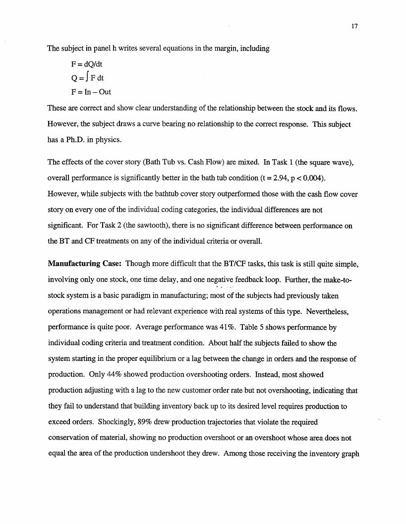
The subject in panel h writes several equations in the margin, including

F = dQ/dt

Q = F dt

F =In - Out

These are correct and show clear understanding of the relationship between the stock and its flows.

However, the subject draws a curve bearing no relationship to the correct response. This subject

has a Ph.D. in physics.

The effects of the cover story (Bath Tub vs. Cash Flow) are mixed. In Task 1 (the square wave),

overall performance is significantly better in the bath tub condition (t = 2.94, p < 0.004).

However, while subjects with the bathtub cover story outperformed those with the cash flow cover

story on every one of the individual coding categories, the individual differences are not

significant. For Task 2 (the sawtooth), there is no significant difference between performance on

the BT and CF treatments on any of the individual criteria or overall.

Manufacturing Case: Though more difficult that the BT/CF tasks, this task is still quite simple,

involving only one stock, one time delay, and one negative feedback loop. Further, the make-to-

stock system is a basic paradigm in manufacturing; most of the subjects had previously taken

operations management or had relevant experience with real systems of this type. Nevertheless,

performance is quite poor. Average performance was 41%. Table 5 shows performance by

individual coding criteria and treatment condition. About half the subjects failed to show the

system starting in the proper equilibrium or a lag between the change in orders and the response of

production. Only 44% showed production overshooting orders. Instead, most showed

production adjusting with a lag to the new customer order rate but not overshooting, indicating that

they fail to understand that building inventory back up to its desired level requires production to

exceed orders. Shockingly, 89% drew production trajectories that violate the required

conservation of material, showing no production overshoot or an overshoot whose area does not

equal the area of the production undershoot they drew. Among those receiving the inventory graph

18

condition, 68% correctly show inventory initially declining, but only 56% show it subsequently

recovering. And 90% drew production paths inconsistent with their inventory trajectory.

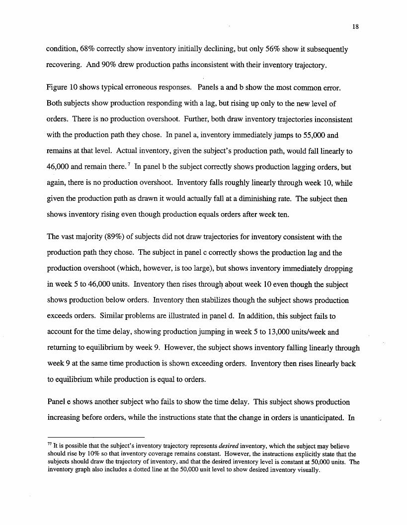
Figure 10 shows typical erroneous responses. Panels a and b show the most common error.

Both subjects show production responding with a lag, but rising up only to the new level of

orders. There is no production overshoot. Further, both draw inventory trajectories inconsistent

with the production path they chose. In panel a, inventory immediately jumps to 55,000 and

remains at that level. Actual inventory, given the subject's production path, would fall linearly to

46,000 and remain there. 7 In panel b the subject correctly shows production lagging orders, but

again, there is no production overshoot. Inventory falls roughly linearly through week 10, while

given the production path as drawn it would actually fall at a diminishing rate. The subject then

shows inventory rising even though production equals orders after week ten.

The vast majority (89%) of subjects did not draw trajectories for inventory consistent with the

production path they chose. The subject in panel c correctly shows the production lag and the

production overshoot (which, however, is too large), but shows inventory immediately dropping

in week 5 to 46,000 units. Inventory then rises through about week 10 even though the subject

shows production below orders. Inventory then stabilizes though the subject shows production

exceeds orders. Similar problems are illustrated in panel d. In addition, this subject fails to

account for the time delay, showing production jumping in week 5 to 13,000 units/week and

returning to equilibrium by week 9. However, the subject shows inventory falling linearly through

week 9 at the same time production is shown exceeding orders. Inventory then rises linearly back

to equilibrium while production is equal to orders.

Panel e shows another subject who fails to show the time delay. This subject shows production

increasing before orders, while the instructions state that the change in orders is unanticipated. In

77 It is possible that the subject's inventory trajectory represents desired inventory, which the subject may believeshould rise by 10% so that inventory coverage remains constant. However, the instructions explicitly state that thesubjects should draw the trajectory of inventory, and that the desired inventory level is constant at 50,000 units. Theinventory graph also includes a dotted line at the 50,000 unit level to show desired inventory visually.

19

addition, the subject's inventory trajectory is inconsistent with the production path. The subject

shows inventory constant through week 5 through production is drawn exceeding orders.

Inventory then falls while production equals orders. This subject reported that he had a Ph.D. in

"nonlinear control theory."

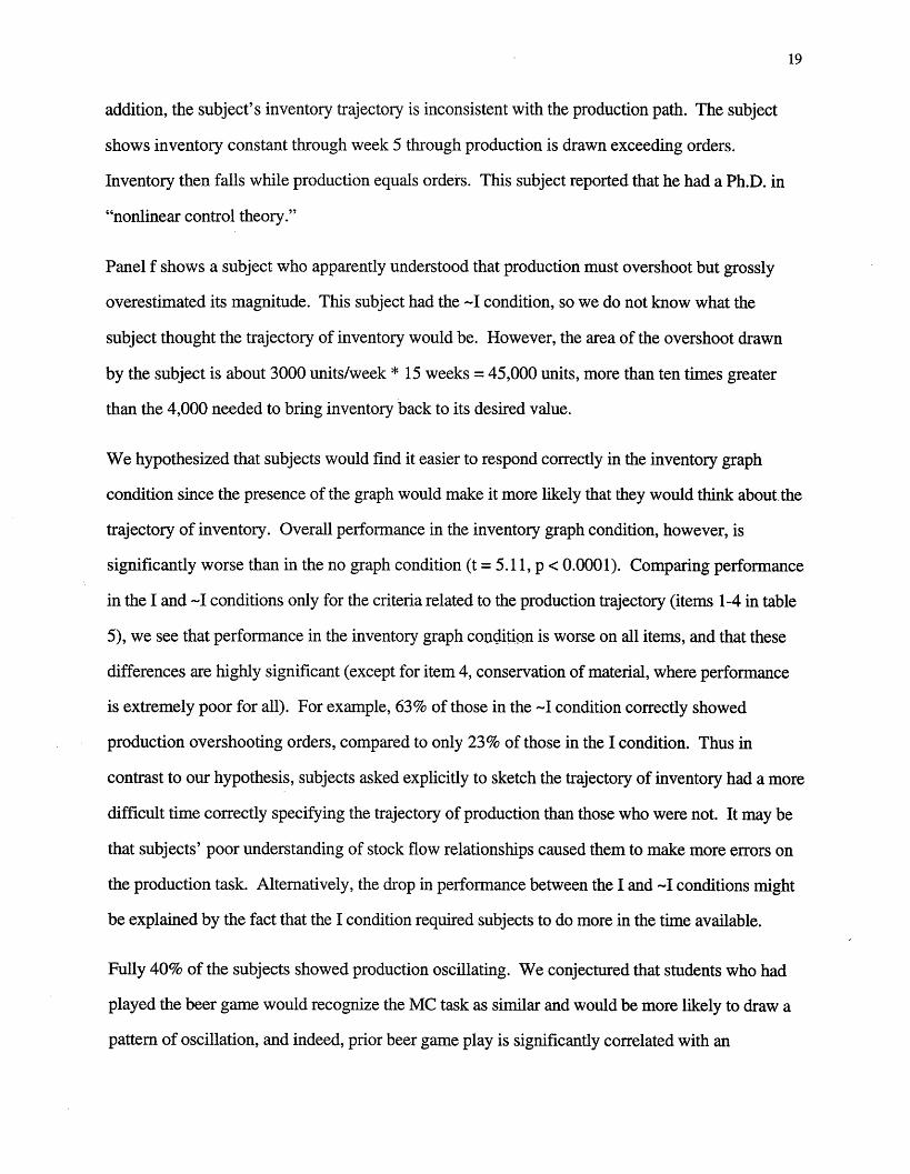
Panel f shows a subject who apparently understood that production must overshoot but grossly

overestimated its magnitude. This subject had the -I condition, so we do not know what the

subject thought the trajectory of inventory would be. However, the area of the overshoot drawn

by the subject is about 3000 units/week * 15 weeks = 45,000 units, more than ten times greater

than the 4,000 needed to bring inventory back to its desired value.

We hypothesized that subjects would find it easier to respond correctly in the inventory graph

condition since the presence of the graph would make it more likely that they would think about the

trajectory of inventory. Overall performance in the inventory graph condition, however, is

significantly worse than in the no graph condition (t = 5.11, p < 0.0001). Comparing performance

in the I and -I conditions only for the criteria related to the production trajectory (items 1-4 in table

5), we see that performance in the inventory graph condition is worse on all items, and that these

differences are highly significant (except for item 4, conservation of material, where performance

is extremely poor for all). For example, 63% of those in the -I condition correctly showed

production overshooting orders, compared to only 23% of those in the I condition. Thus in

contrast to our hypothesis, subjects asked explicitly to sketch the trajectory of inventory had a more

difficult time correctly specifying the trajectory of production than those who were not. It may be

that subjects' poor understanding of stock flow relationships caused them to make more errors on

the production task. Alternatively, the drop in performance between the I and -I conditions might

be explained by the fact that the I condition required subjects to do more in the time available.

Fully 40% of the subjects showed production oscillating. We conjectured that students who had

played the beer game would recognize the MC task as similar and would be more likely to draw a

pattern of oscillation, and indeed, prior beer game play is significantly correlated with an

20

oscillatory production path (Pearson r = 0.24, p = 0.0004). About 48% of those who had played

the beer game showed production oscillating compared to only 35% of those who had not played

the game. Interestingly, subjects who had played the beer game did significantly better on the MC

task compared to those who had not (average score of 46% vs. 33%, t = 3.35, p < 0.001). There

are two competing explanations for the improvement. It may be that playing the beer game gave

students insight into the dynamics of the stock management system, so that their higher score

indicates that they learned important lessons about delays and stocks and flows. Alternatively,

those who had played the game may have remembered the behavior without gaining much

appreciation for the underlying stock and flow principles. Specifically, they may recall that in the

game production oscillated and that their inventory initially declined, then increased. Any pattern

of oscillation necessarily shows production overshooting the order rate, one of the key

requirements of a correct response. Similarly, subjects who drew inventory falling and then rising

as in the beer game would receive credit for correctly identifying the qualitative behavior of

inventory (items 5 and 6 in Table 5). Figure 11 shows a typical response in which production is

shown as oscillating around the order rate. The subject writes in the margin "Some sort of wild

variation (this is the beer game, right?)." The subject's response shows no apparent understanding

of the stock and flow relationships that require production to overshoot-overshoot is an artifact of

the "wild variation."

Close analysis of the results suggests subjects drawing an oscillation did better as an artifact of

drawing an oscillatory response without having any greater understanding of inventory

management or stocks and flows (Table 5). Fifty-three percent of those with beer game experience

received credit for showing the production overshoot compared to only 30% of those without beer

game experience, a significant difference ( 2 = 11.5, p = 0.001). Similarly, those with beer game

experience did significantly better at showing an initial decline and subsequent recovery in

inventory (77% vs. 55% for the initial decline, X2 = 6.1, p = 0.01, and 66% vs. 43% for the

subsequent recovery, 2 = 5.6, p = 0.02). However, there was no significant difference on items

1, 2, 4, and 7. These include conformance with the conservation law and consistency of the

21

production and inventory trajectory. Further, as shown in Table 6, prior beer game experience is

significantly related to performance in the MC task but not to performance in either BT/CF tasks.

These results suggest subjects with beer game experience received credit for the production

overshoot and inventory decline as artifacts of drawing oscillatory trajectories, but have no better

understanding of key attributes of stock and flow structures, including conservation of material and

consistency of the net flow and change in the stock.

Impact of Subject Demographics: It is plausible to expect that prior education should affect

performance. In particular, we hypothesized that subjects with more training in mathematics, the

sciences, or engineering would outperform those with training in the social sciences or humanities.

To test this hypothesis we ran a variety of general linear models relating performance on the

different tasks to the various demographic variables subjects reported. Table 6 reports models in

which performance on each task is explained by highest prior degree and major field, current

academic program, gender, age, region of origin, English as a native language, and prior beer

game play (defined as in Table 1). While some items are significant, there is no consistent pattern.

Prior academic field is significant for BT/CF Task 1, and highest prior degree is marginally

significant, and, as hypothesized, those with technical backgrounds do better than those in the

social sciences, but these factors are far from significant in the other tasks. The degree program in

which students were currently enrolled was not significant in any of the tasks. The results provide

only limited support for the hypothesis that prior training in the sciences helps performance. It is

possible that there simply is insufficient variation in the subject pool to detect any effects. Other

demographic factors also appear to have only a weak impact. Age is not significant. Performance

did not depend on whether English was the subject's first language, but region of origin is

significant for BT/CF Task 1, and marginally significant in BT/CF 2 and the MC task. Subjects

from North America generally did better. There is a suggestion of a gender effect. Males

outperform females on all three tasks, though the effect is only marginally significant.

22

5 DISCUSSION

The results strongly suggest that highly educated subjects with extensive training in mathematics

and science have poor understanding of some of the most basic concepts of system dynamics,

specifically, stocks and flows, time delays, and feedback. The errors are highly systematic, and

indicate violations of basic principles, not merely calculation errors. Subjects tend to violate

fundamental relationships between stocks and flows, including conservation of matter, as shown

by the large fraction of respondents in the MC task who drew trajectories for production and

inventory that were inconsistent with one another. This result is further reinforced by the

significant deterioration in results between BT/CF Task 1 and BT/CF Task 2: Subjects have poor

understanding of the relationship between the net flow into a stock and the slope of the stock

trajectory. Many subjects do not understand the relationship between the area enclosed by the net

rate into a stock over some interval and the change in the stock over the interval.

Many subjects appear to believe that the stock trajectory should have the same qualitative shape as

the net rate. In BT/CF Task 1, the net rate is discontinuous, and 1% of the subjects drew stock

trajectories that were also discontinuous, similar to the subject shown in Figure 8 a. In BT/CF

Task 2, the net rate is continuous, and only 2 of 150 (1.3%) of the subjects drew discontinuous

trajectories for the stock, the only criterion on which the subjects did better on Task 2 than Task 1.

However, 72 of 150 subjects in Task 2 (48%) drew stock trajectories with discontinuous slopes,

similar to the net rate (as illustrated by Figure 9a). We conjecture that subjects with weak

understanding rely on a heuristic that matches the shape of the output of the system to the shape of

the input. To illustrate how far wrong such intuitive matching is, plot the derivative of the stock

trajectories in figures 8 and 9 and compare them to the actual net rate.

The two features that subjects find problematic-the slope of the stock is the net flow, and the

change in the stock over an interval is the area enclosed by the net rate in that interval-are the two

fundamental concepts of the calculus. One might argue that calculus represents rather advanced

mathematics, so the failure of the subjects to do well on these tasks is not too worrisome. Such a

23

view, we believe, is erroneous. First, essentially every subject in our experiments had taken

calculus (it is a prerequisite for admission to the Sloan School). Many had years of coursework

and even undergraduate or graduate degrees in mathematics, engineering, or the sciences.

Nevertheless, there is only a weak relationship between education and performance. For a large

fraction of the subjects, training and experience with calculus and mathematics did not translate into

an intuitive appreciation of accumulations, of stocks and flows.

More importantly, these tasks do not require subjects to use any of the analytic tools of calculus; no

derivatives need be taken, no integrals written or evaluated. The tasks can be answered without

use of any mathematics beyond simple arithmetic (and perhaps the formulae for the area of

rectangles and triangles). The concepts of accumulation, though formalized in the calculus, are

common and familiar to all of us through a host of everyday tasks, including filling a bathtub,

managing a checking account, or controlling an inventory.

We turn now to consider alternative explanations for the results. One possibility is that the subjects

did not put much effort into the tasks because there was insufficient incentive. Economists

generally argue that subjects should be paid in proportion to performance in experiments and

question results in which performance incentives are weak (Smith 1982). In a review of more than

70 studies, Camerer and Hogarth (1999) found incentives sometimes improved performance. In

other cases even significant monetary incentives did not improve performance or eliminate

judgmental errors. In some cases incentives worsened performance. It is possible that additional

incentive in the form of grades or monetary payment would improve the results. On the other

hand, if we ask students "What is 2 + 2?" essentially all answer "four" without hesitation even

without grades or payment. The knowledge required in our experiment is nearly as basic and

should be nearly as automatic. The resolution of this issue awaits future research.

It is also possible that the subjects were given insufficient time. This question also must be left for

future research. We expect that more time would improve performance, but suspect many of the

same errors will persist, particularly violations of conservation laws and inconsistent net rate and

24

stock trajectories. Given the importance and ubiquity of stock and flow structures people should

be able to infer their dynamics quickly and reliably; their failure to do so even in a relatively short

period of time is a further indicator of their poor understanding of these critical concepts.

Advocates of the naturalistic decision making movement argue that many of the apparent errors

documented in decision making research arise not because people have poor reasoning skills but as

artifacts of unfamiliar and unrealistic laboratory tasks. While strongly emphasizing the bounded

rationality of human decision making, they argue that people can often perform well in complex

decision making settings because we have evolved "fast and frugal" heuristics that "are successful

to the degree they are ecologically rational, that is, adapted to the structure of the information in the

environment in which they are used..." (Gigerenzer et al. 1999, vii). Perhaps people understand

stocks, flows, delays, and feedback well and can use them in everyday tasks, but do poorly here

because of the unfamiliar and unrealistic presentation of the problems. After all, people do manage

to fill and drain their bathtubs and manage their checking accounts. We agree that people can

perform well in familiar, naturalistic settings yet poorly on the same type of task in an unfamiliar

setting. Our decision making capabilities evolved to function in particular environments; to the

extent the heuristics we use in these environments are context-specific, performance will not

necessarily transfer to other situations even if their logical structure is the same.

What is the naturalistic context for this type of task? More and more of the pressing problems

facing us as managers and citizens alike involve long delays. The long time scale for the

consequences of many decisions means there is little opportunity for learning through outcome

feedback and thus for the evolution of high-performing decision rules (Sterman 1994).

Increasingly, we are faced with tasks involving significant stocks and flows, time delays, and

feedbacks, tasks for which the naturalistic context is a spreadsheet, a graph, or a text-the same

type of presentation in our tasks. Managers are called on to evaluate spreadsheets and graphs

projecting revenue and expenditure, bookings and shipments, hiring and attrition. These modes of

data presentation are not unique to business. Epidemiologists must understand the relationship

25

between the incidence and prevalence of disease, urban planners need to know how migration and

population are related, and everyone, not only climatologists, needs to understand how emissions

of greenhouse gases affect their concentration in the atmosphere and how that concentration in turn

alters heat flux and global temperatures. For many of the most pressing issues in business and

public policy, the mode of data presentation in our tasks is the naturalistic context.

There is abundant evidence that sophisticated policymakers suffer from the same errors in

understanding stocks and flows we observe in our experiments. To take only one example,

Homer (1993) used basic stock-flow logic to show that US government survey data on the

prevalence of cocaine use could not be correct. The number of people who reported that they had

used cocaine in the past month showed a sharp drop starting around the late 1980s. Yet at the

same time cocaine related arrests, medical emergencies, and deaths were growing exponentially,

while prices fell and purity increased, suggesting rising use. Which data were correct? The

government also asks survey respondents if they have ever used cocaine. However, these lifetime

prevalence estimates were not much discussed in policy circles because they did not distinguish

between current and former users. Homer realized, however, that this feature meant the lifetime

prevalence estimates could be used to provide a strong check on the accuracy of the survey data.

The number of people who have ever used cocaine is a stock increased by the rate at which people

try the drug for the first time. It is decreased only by death. The reported decline in lifetime

prevalence was physically impossible-even if everyone in the country "just said no," cutting the

inflow of new users to zero, lifetime prevalence could not decline that fast. The survey assumed,

however, that the fraction of people responding truthfully was constant and that the sample was

properly stratified. Instead, as people realized that cocaine was actually harmful, and as its social

and legal acceptability fell, more and more current and former users simply lied about their drug

use. Further, since heavy cocaine users were more likely to be homeless or live in poor and

dangerous neighborhoods, they were less likely to be included in the survey. Homer showed that

the actual population of people who had ever used cocaine must have continued to grow, although

26

at a diminishing rate, and likely reached more than 60 million people by 1995, compared to the

government's estimate of about 25 million. Until Homer's work no one in the drug policy

establishment pointed out the inconsistency. These results had large public policy implications,

since the Bush administration used the erroneous survey data showing large drops in cocaine use

to argue that the war on drugs, with its focus on interdiction and incarceration rather than

prevention, was working. Billions of dollars were spent on such interdiction efforts, but, as

MacCoun and Reuter (1997, p. 47) put it, "The probability of a cocaine or heroin seller being

incarcerated has risen sharply since about 1985 but that has led neither to increased price nor

reduced availability."

Assuming our results withstand replication and additional testing, what are the implications for

system dynamicists and teachers interested in developing the systems thinking capabilities of their

clients and students? It appears that we should spend considerable time on the basics of stocks and

flows, time delays, and feedback, with an emphasis on developing intuition rather than the

mathematics. Of course, we believe the mathematics and formal theory are important, and no good

system dynamics education can do without them. But our results suggest that good mathematics

training alone is not sufficient to develop a practical, common-sense understanding of the most

basic building blocks of complex systems. We suggest students should be given extensive

opportunities for hands-on practice in both identifying and mapping stock and flow structures and

graphical integration and differentiation.

Our results also suggest implications beyond system dynamics curriculum and pedagogy. We

found that students have difficulty with basic concepts of great importance in many disciplines and

real-world tasks. These findings mirror similar results that learners hold many misconceptions

about a variety of concepts such as probability or Newton's laws (Grotzer 1993, Grotzer and Bell

1999). Several decades of research in science education show that many students hold intuitive

theories quite different from those of scientists, and that these ideas are highly resistant to change

(Sadler, 1998). These beliefs are not limited to naivete about physical principles such as 'heavy

27

objects fall faster than light ones' but include a staggering array of magical and superstitious beliefs

antithetical to the principles of scientific method itself (Sterman 1994). System dynamics educators

can learn much from attempts to overcome these misconceptions in science and mathematics

education.

At the same time, educators in the K-12 arena can also learn from our results. Frankly, the

concepts of accumulations and time delays are so basic they should already be well understood by

the time students reach college, much less graduate school. As system dynamics educators, we

should not have to take valuable class time to teach what are, essentially, remedial lessons on how

accumulations work, how to read graphs, and so on. This is not merely a problem about

dynamics. A recent study by the American Association for the Advancement of Science reviewed

popular algebra texts used in US schools. The panel concluded that the reason students aren't

learning the concepts of algebra is that the books (and by implication, the curricula and pedagogy)

"don't explain how algebra calculations will relate to everyday life" according to the Boston Globe

(27 April 2000, p. A27). In rating the texts the panel found none of them to be excellent.

"Five-including the three most widely used in American classrooms-were rated so inadequate

that they lack potential for student learning."

Of course our results are preliminary and much more work is needed. We are developing

additional items to assess other dimensions of complexity such as the ability to recognize and

interpret feedback relationships, the ability to recognize and analyze nonlinear relationships

between cause and effect, and the ability to estimate and analyze the impact of time delays.

There is additional work to be done exploring how performance depends on factors such as

gender, prior education and experience, and other demographic variables. We plan to expand the

subject pool to include a broader range of people, from K-12 students to experienced managers.

Differences in performance among these groups may provide important clues to the source of

people's learning about these concepts. Interviews and verbal protocols have proven productive in

prior evaluative research on students' alternative conceptions of scientific principles (Sadler 1998,

28

Duckworth 1987, Osborne and Gilbert 1980), and we expect such tools will be useful in

understanding the sources of student difficulties with systems thinking concepts as well.

The inventory should help educators and researchers establish a baseline measure of people's

ability to understand the elements of dynamic complexity and use them effectively in everyday

reasoning. It also provides a preliminary tool to measure the impact of various types of systems

thinking training. Ultimately, evaluative research on the efficacy of systems thinking training and

interventions should assess whether and how an intervention affected the behavior of the

participants and the outcomes of new policies and actions taken as a result, not only changes in

their attitudes, thinking, and skills.

29

References

Ackoff, R. & Gharajedaghi, J., (1985). Toward Systemic Education of Systems Scientists,Systems Research, 2(1), 21-27.

Bakken, B. E., J. M. Gould, et al. (1992) Experimentation in Learning Organizations: AManagement Flight Simulator Approach, European Journal of Operations Research 59(1), 167-182.

Boutilier, R. (1981). The Development of Understanding of Social Systems. PhD Thesis, TheUniversity of British Columbia, British Columbia.

Brehmer, B. (1992) Dynamic decision making: Human control of complex systems, ActaPsychologica 81, 211-241.

Camerer, C. and R. Hogarth (1999) The effects of financial incentives in experiments: A reviewand capital-labor-production framework. Journal of Risk and Uncertainty 19(1-3), 7-42.

Cavaleri, S. and J. Sterman (1997) Towards evaluation of systems thinking interventions: A casestudy, System Dynamics Review 13(2), 171-186.

Chandler, M. and R. Boutilier (1992). The Development of Dynamic System Reasoning.Contributions to Human Development 21, 121-137.

Dangerfield, B. C. and C. A. Roberts (1995). Projecting Dynamic Behavior in the Absence of aModel: An Experiment, System Dynamics Review 11(2), 157-172.

Diehl, E. and J. Sterman (1995) Effects of feedback complexity on dynamic decision making,Organizational Behavior and Human Decision Processes 62(2), 198-215.

D6rner, D. (1980) On the difficulties people have in dealing with complexity, Simulations andGames 11(1), 87-106.

D6rner, D. (1996) The Logic of Failure. New York: Metropolitan Books/Henry Holt.

Doyle, J., M. Radzicki, and S. Trees (1996) Measuring the Effect of System ThinkingInterventions on Mental Models. 1996 International System Dynamics Conference,Cambridge, Massachusetts, System Dynamics Society, 129-132.

Doyle, J., M. Radzicki, and S. Trees (1998) Measuring Changes in Mental Models of DynamicSystems: An Exploratory Study. 16th International Conference of the System DynamicsSociety, Quebec '98, Quebec City, Canada, System Dynamics Society.

Duckworth, E. (1996) The Having of Wonderful Ideas and Other Essays on Teaching andLearning, New York: Teacher's College Press.

Forrester, J. W. (1961) Industrial Dynamics. Cambridge: MIT Press; Currently available fromPegasus Communications: Waltham, MA.

Frensch, P. A. and J. Funke, Eds. (1995). Complex Problem Solving - The EuropeanPerspective. Mahwah, Lawrence Erlbaum Associates, Inc.

Gigerenzer, G., P. Todd, et al. (1999) Simple Heuristics that Make Us Smart. New York:Oxford University Press.

Gould, J., (ed.) (1993) Systems Thinking in Education, System Dynamics Review (special issue)9(2).

Grotzer, Tina. (1993). Children's Understanding of Complex Causal Relationships in NaturalSystems. Harvard Graduate School of Education. Cambridge, Harvard University.

30

Grotzer, T.A. & Bell, B. (1999). Negotiating the funnel: Guiding students toward understandingelusive generative concepts. In L. Hetland & S. Veenema (Eds.) The Project Zero Classroom:Views on Understanding. Cambridge, MA: Fellows and Trustees of Harvard College.

Homer, J. (1993) A system dynamics model of national cocaine prevalence, System DynamicsReview 9(1), 49-78.

MacCoun, R. and P. Reuter (1997) Interpreting Dutch cannabis policy: Reasoning by analogy inthe legalization debate, Science 278 (3 Oct), 47-52.

Mandinach, E. and H. Cline (1994) Classroom Dynamics: Implementing a Technology-BasedLearning Environment. Hillsdale, NJ: Lawrence Erlbaum Associates.

Microworlds Inc. Brochure, 1997, Divsion of GKA Inc., Cambridge, Massachusetts 02138.

Osborne, R., & Gilbert, J. (1980) A technique for exploring students' views of the world,Physics Education, 15, 376 - 379.

Ossimitz, Gunther, (1996). Development of Systems Thinking. Institute of Educational Research,Bonn, Germany.

Paich, M. and J. Sterman (1993) Boom, bust, and failures to learn in experimental markets,Management Science 39(12), 1439-1458.

Richmond, B. (1993) Systems thinking: Critical thinking skills for the 1990s and beyond, SystemDynamics Review 9(2), 113-134.

Sadler, P. (1998) Pyschometric Models of Student Conceptions in Science: ReconcilingQualitiative Studies and Distractor-Driven Assessment Instruments. Journal of Research inScience Teaching 35(3), 265-296.

Senge, P. (1990) The Fifth Discipline: The Art and Practice of the Learning Organization. NewYork: Doubleday.

Senge, P. et al. (1999) The Dance of Change: The Challenges to Sustaining Momentum inLearning Organizations. New York: Doubleday.

Smith, V. (1982) Microeconomic systems as an an experimental science, American EconomicReview, 72, 923-955.

Sterman, J. (1989a) Misperceptions of feedback in dynamic decision making. OrganizationalBehavior and Human Decision Processes 43(3), 301-335.

Sterman, J. (1989b) Modeling managerial behavior: Misperceptions of feedback in a dynamicdecision making experiment, Management Science 35(3), 321-339.

Sterman, J. (1994) Learning In and About Complex Systems, System Dynamics Review 10(2-3),291-330.

Sterman, J. (2000) Business Dynamics: Systems Thinking and Modeling for a Complex World.New York: Irwin/McGraw-Hill.

TLC Team Learning Lab brochure, 1998. The Learning Circle, Sudbury, Massachusetts.

Vennix, J. (1996). Group Model Building: Facilitating Team Learning Using System Dynamics.Chichester: Wiley.

Zulauf, Carol. A. (1995). An Exploration of the Cognitive Correlates of Systems Thinking. Ph. D.Thesis, Boston University, Boston, MA.

31

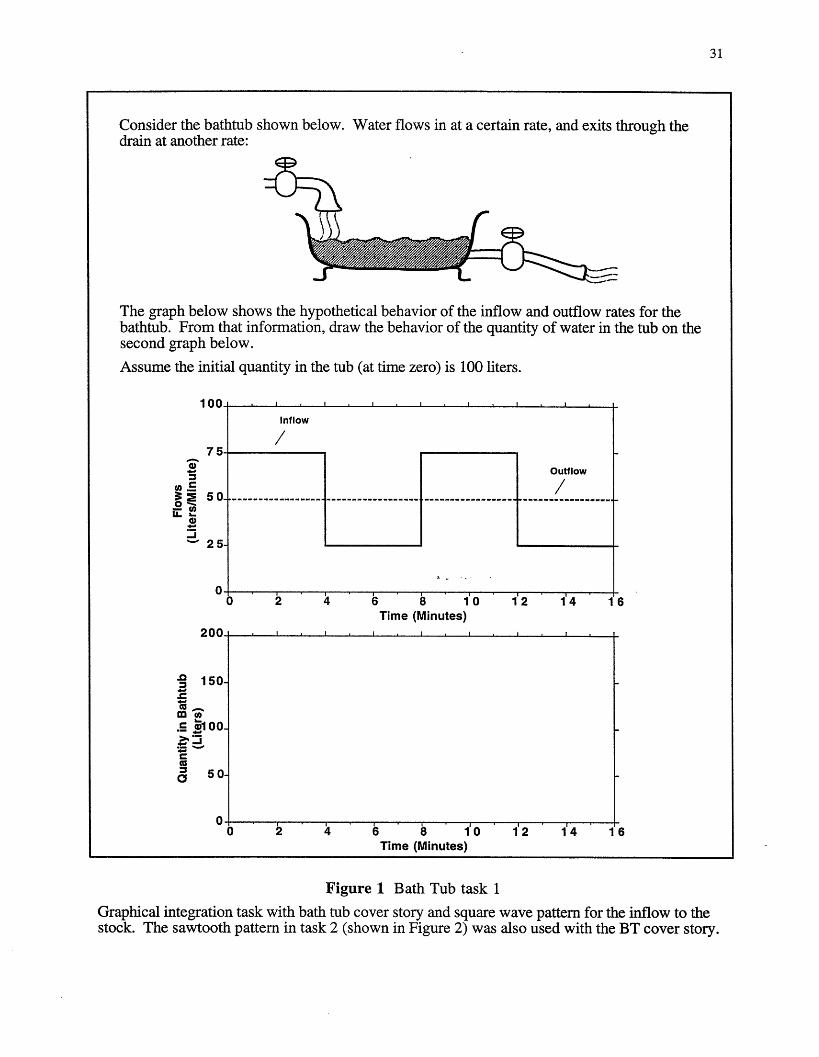
Consider the bathtub shown below. Water flows in at a certain rate, and exits through thedrain at another rate:

The graph below shows the hypothetical behavior of the inflow and outflow rates for thebathtub. From that information, draw the behavior of the quantity of water in the tub on thesecond graph below.

Assume the initial quantity in the tub (at time zero) is 100 liters.

a .)

3 E

0-

-j

n.=

am

100. , .i

Inflow

/75

Outflow

25-

00 2 4 6 8 1'0 12 1'4 1

Time (Minutes)200 ,

150-

1 00

50-

00 2 4 6 8 10 12 14 1

Time (Minutes)

Figure 1 Bath Tub task 1

Graphical integration task with bath tub cover story and square wave pattern for the inflow to thestock. The sawtooth pattern in task 2 (shown in Figure 2) was also used with the BT cover story.

i

32

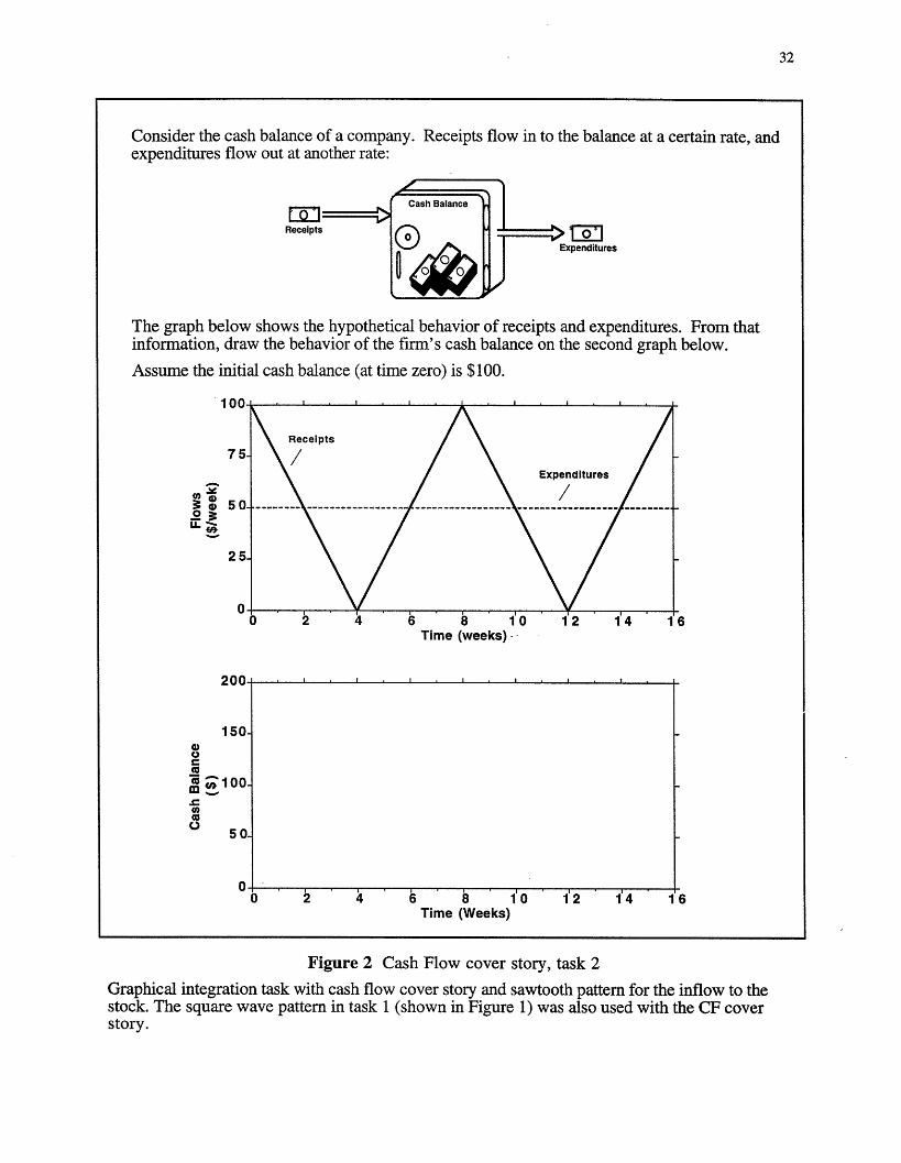
Consider the cash balance of a company. Receipts flow in to the balance at a certain rate, andexpenditures flow out at another rate:

Receipts

xpenditures

The graph below shows the hypothetical behavior of receipts and expenditures. From thatinformation, draw the behavior of the firm's cash balance on the second graph below.

Assume the initial cash balance (at time zero) is $100.

Time (weeks) -

ZUU. I I20 g - f , . I , , * .*

150-

100

50

0 i

0 2 4 6 8Time (Weeks'

10 12 14

Figure 2 Cash Flow cover story, task 2

Graphical integration task with cash flow cover story and sawtooth pattern for the inflow to thestock. The square wave pattern in task 1 (shown in Figure 1) was also used with the CF coverstory.

1(

7

2

4A)

5

2

3

(D0C_ma

o0

*

1 6

~AA

' Ann

- 150-

a 50.C

4 6, 8 1'0Time (Minutes)

0 i 4 6 8 10Time (Minutes)

1'2 ' 14

12 14

Figure 3. A subject response showing the correct answer to BT /CF Task 1.

Time (weeks)

200- . . . . . . . . . . . . . .

150

100

50-1 W

0 2 4 6 8 10 12 "14'Time (Weeks)

Figure 4. A subject response showing the correct answer to BT /CF Task 2.

Itnn

33

_

jo -,-U

.It-

75.

50-

25.

Inflow

/

2T -oo -Outflow. -/o /

16

6

0

co

r

o)0C,

In

U

6

VU .............. - - - i i , i i

LUU -i - .-- --

I

. _0

1. _

- -

ot:,v W.,! -

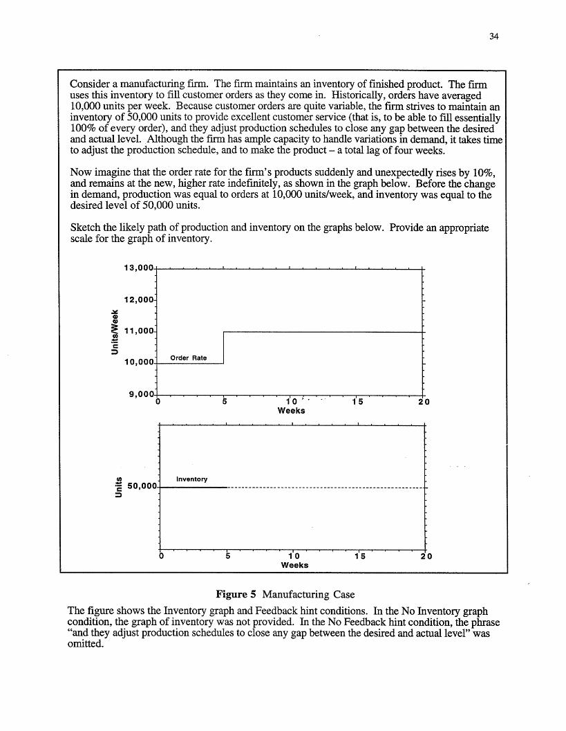
34

Consider a manufacturing firm. The firm maintains an inventory of finished product. The firmuses this inventory to fill customer orders as they come in. Historically, orders have averaged10,000 units per week. Because customer orders are quite variable, the firm strives to maintain aninventory of 50,000 units to provide excellent customer service (that is, to be able to fill essentially100% of every order), and they adjust production schedules to close any gap between the desiredand actual level. Although the firm has ample capacity to handle variations in demand, it takes timeto adjust the production schedule, and to make the product - a total lag of four weeks.

Now imagine that the order rate for the firm's products suddenly and unexpectedly rises by 10%,and remains at the new, higher rate indefinitely, as shown in the graph below. Before the changein demand, production was equal to orders at 10,000 units/week, and inventory was equal to thedesired level of 50,000 units.

Sketch the likely path of production and inventory on the graphsscale for the graph of inventory.

Ill nnn

12,000-

a)

11,000-

. n nnn

9,000-

(a

'r

O

0

5 1'0 .. -' 1'5

Weeks

10Weeks

below. Provide an appropriate

20

201 5

Figure 5 Manufacturing Case

The figure shows the Inventory graph and Feedback hint conditions. In the No Inventory graphcondition, the graph of inventory was not provided. In the No Feedback hint condition, the phrase"and they adjust production schedules to close any gap between the desired and actual level" wasomitted.

Order Rate

Inventory

,VVV.

. . ...

· · · · · · · · · · · · · · · ·

VVV' ------

I I · · I · · I · i · · --· · i i i · I

I

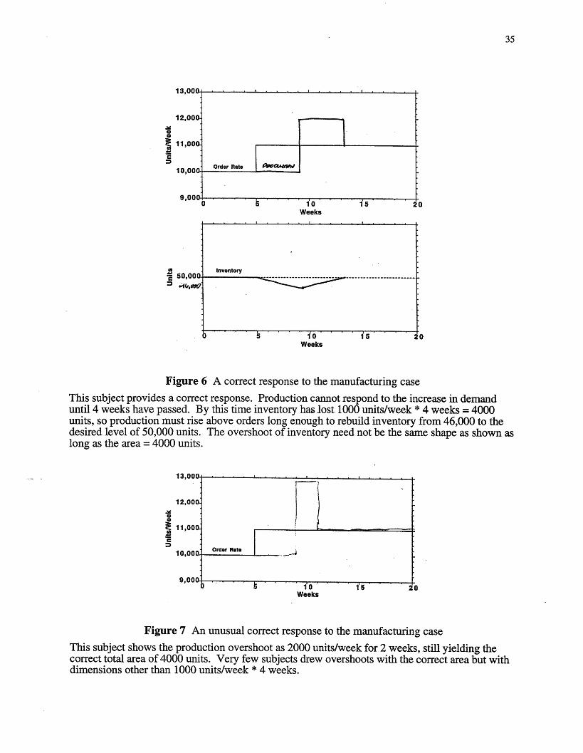
35

a0

0

Weeks, · . . I . . . . .

- 50,000

0 5 1 0Weeks

is 20

Figure 6 A correct response to the manufacturing case

This subject provides a correct response. Production cannot respond to the increase in demanduntil 4 weeks have passed. By this time inventory has lost. 1000 units/week * 4 weeks = 4000units, so production must rise above orders long enough to rebuild inventory from 46,000 to thedesired level of 50,000 units. The overshoot of inventory need not be the same shape as shown aslong as the area = 4000 units.

0

I

13,000 . . .. .

12,000

11,000

Order Rate10,000 _J

9,000 ..IQ0 I - *

Weeks

Figure 7 An unusual correct response to the manufacturing case

This subject shows the production overshoot as 2000 units/week for 2 weeks, still yielding thecorrect total area of 4000 units. Very few subjects drew overshoots with the correct area but withdimensions other than 1000 units/week * 4 weeks.

Inventory------------------------ - -------------------

. ~ --· . .- * . . . . . . . . . . I

.I_ dE n

36

Group 1 Group 1 Group 2All entries are % Session 1 Session 2 Session 1

MC & PFd BT/CF T BT/CF T2n = 225 n = 143 n = 150

Age 19-24 14 13 1025-30 53 49 5931-35 30 34 2036 and up 4 4 11

Gender M 73 71 76F 27 29 24

Student Statuslst/2nd yr. MBA 56 56 37Executive MBA" 11 11 16LFMb 8 10 16Otherc 25 24 32

Prior Field of StudyBusiness/Management 17 16 27Engineering 40 43 45Social Sciences 23 22 4Science 7 5 10Computer Science 6 7 5Math 4 4 6Humanities 2 3 4

Highest Prior DegreeBA 22 23 17BS 35 36 43MA/MS 30 27 28Ph.D 6 7 5High school 2 2 2BE, JD, BBA, MD 2 - 2 1BA & BS 3 3 3

Region of OriginNorth America (+ Aus./NZ) 35 36 50Europe 19 20 16Asia and Middle East 32 29 22Latin America 13 14 10Africa 1 1 2English First language 44 44 54

Not first language 56 56 46Beer Game ExperiencePlayed before 61 62 62Have not played 39 38 38

a The executive MBA students were enrolled in a various one-year degree programs at MIT and are typically mid-career executives with extensive business experience.

b LFM = Leaders for Manufacturing, a dual degree program awarding both an MBA and MS in engineering.c 'Other' includes Ph.D. and graduate students from other MIT departments (averaging about 12%), graduate

students from other universities (primarily Harvard), averaging about 10%, and MIT undergraduates (about 5%).d PF = Paper Fold task, the results of which are not described in this paper. See note 5.Totals may not equal 100% due to rounding.

Table 1 Subject demographics

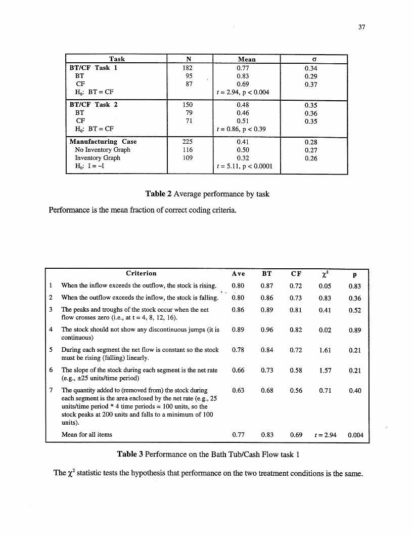
37

Table 2 Average performance by task

Performance is the mean fraction of correct coding criteria.

Criterion Ave BT CF X2 P

1 When the inflow exceeds the outflow, the stock is rising.

2 When the outflow exceeds the inflow, the stock is falling.

3 The peaks and troughs of the stock occur when the netflow crosses zero (i.e., at t = 4, 8, 12, 16).

4 The stock should not show any discontinuous jumps (it iscontinuous)

5 During each segment the net flow is constant so the stockmust be rising (falling) linearly.

6 The slope of the stock during each segment is the net rate(e.g., +25 units/time period)

7 The quantity added to (removed from) the stock duringeach segment is the area enclosed by the net rate (e.g., 25units/time period * 4 time periods = 100 units, so thestock peaks at 200 units and falls to a minimum of 100units).

Mean for all items

0.80 0.87 0.72 0.05 0.83

0.80 0.86 0.73 0.83 0.36

0.86 0.89 0.81 0.41

0.89 0.96 0.82 0.02

0.52

0.89

0.78 0.84 0.72 1.61 0.21

0.66 0.73 0.58 1.57 0.21

0.63 0.68 0.56 0.71 0.40

0.77 0.83 0.69 t = 2.94 0.004

Table 3 Performance on the Bath Tub/Cash Flow task 1

The x2 statistic tests the hypothesis that performance on the two treatment conditions is the same.

Task N Mean aBT/CF Task 1 182 0.77 0.34

BT 95 0.83 0.29CF 87 0.69 0.37H0 : BT = CF t = 2.94, p < 0.004

BT/CF Task 2 150 0.48 0.35BT 79 0.46 0.36CF 71 0.51 0.35Ho: BT = CF t = 0.86, p < 0.39

Manufacturing Case 225 0.41 0.28No Inventory Graph 116 0.50 0.27Inventory Graph 109 0.32 0.26Ho: I =-I t = 5.11, p < 0.0001

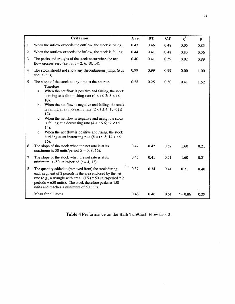
38

Criterion

1 When the inflow exceeds the outflow, the stock is rising.

2 When the outflow exceeds the inflow, the stock is falling.

3 The peaks and troughs of the stock occur when the netflow crosses zero (i.e., at t = 2, 6, 10, 14).

4 The stock should not show any discontinuous jumps (it iscontinuous)

5 The slope of the stock at any time is the net rate.Therefore

a. When the net flow is positive and falling, the stockis rising at a diminishing rate (0 < t < 2; 8 < t <10).

b. When the net flow is negative and falling, the stockis falling at an increasing rate (2 < t < 4; 10 < t <12).

c. When the net flow is negative and rising, the stockis falling at a decreasing rate (4 < t < 6; 12 < t <14).

d. When the net flow is positive and rising, the stockis rising at an increasing rate (6 < t < 8; 14 < t <16).

6 The slope of the stock when the net rate is at itsmaximum is 50 units/period (t = 0, 8, 16).

Ave BT CF P

0.47 0.46 0.48 0.05 0.83

0.44 0.41 0.48 0.83 0.36

0.40 0.41 0.39 0.02 0.89

0.99 0.99 0.99 0.00 1.00

0.28 0.25 0.30 0.41 1.52

0.47 0.42 0.52 1.60 0.21

7 The slope of the stock when the net rate is at itsminimum is -50 units/period (t = 4, 12).

8 The quantity added to (removed from) the stock duringeach segment of 2 periods is the area enclosed by the netrate (e.g., a triangle with area ±(1/2) * 50 units/period * 2periods = +50 units). The stock therefore peaks at 150units and reaches a minimum of 50 units.

Mean for all items

0.45 0.41 0.51

0.37

1.60 0.21

0.34 0.41 0.71 0.40

0.48 0.46 0.51 t = 0.86 0.39

Table 4 Performance on the Bath Tub/Cash Flow task 2

Flows(S/Week)

Cash Balance Flows(S/Week)

0

A

=1Cab

a9HC

CDO-t

-t

cD00-t

CD

co9rjI

CD

cd0H

HnCDrA

Cn

-q

Ca

-40IF0

.0iCa

/ -/

/

/

/

/

/

rC ,i ,

v/ ns

a/

Quantity in BathtubILittartl

Quantity in Bathtub(Lites)

a o 0 0

. vI o

CA -

0

. -0

.3.

0SrI

Flows(Liters/Minute)

:ja0

(3CA

B3

.51C

0

0CI=

c0

CDCD

0

T1rH"ta

CD

o

CD

cn

T

Flows(Liters/Mlnute)O a0Mn 0

-4 0cn 1o

I-

_r

J\o0 to

'.1 .

tQ IJ 0 o~ t

%rA~ X~'M40 -,~

0j

4 b.S

D

0

Im

S

-I- z-

. i

(IC

P44.

II

V

0

.,. 1 I · CI.- --- · -.----,-------4. , _

N0O

--1

1 I I4 nx

.

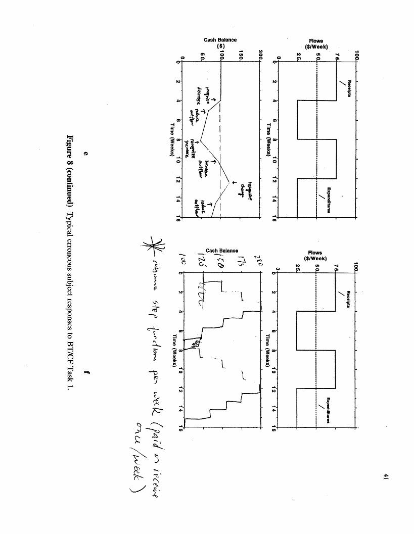
Cash Balance Flows

-4

rIQ

cc

OF

-Iz

-30

0XA

($/Week).

-

0

o 4 _Cash Balance Flows0z -. , -c A ($/Week)CD- :IT- ~ v-,% 1'

I., ''~ 7::' Cr --'

WP II:=

rjr

r. r-11

o3 _

A t

C,

-".

3

-0M0

0

N..N

X,-

Quantity in Bathtub'(liters) -

3ID

3

vCiMA

r

CDI0(D

0C,CD

.I13P:

=t3

IDMcDMW

Cash Balance($)

-I

3aD

Cor

! lows

(liters/minute)

Flows($/week)

-I3

Co

t'-NI

t

cn

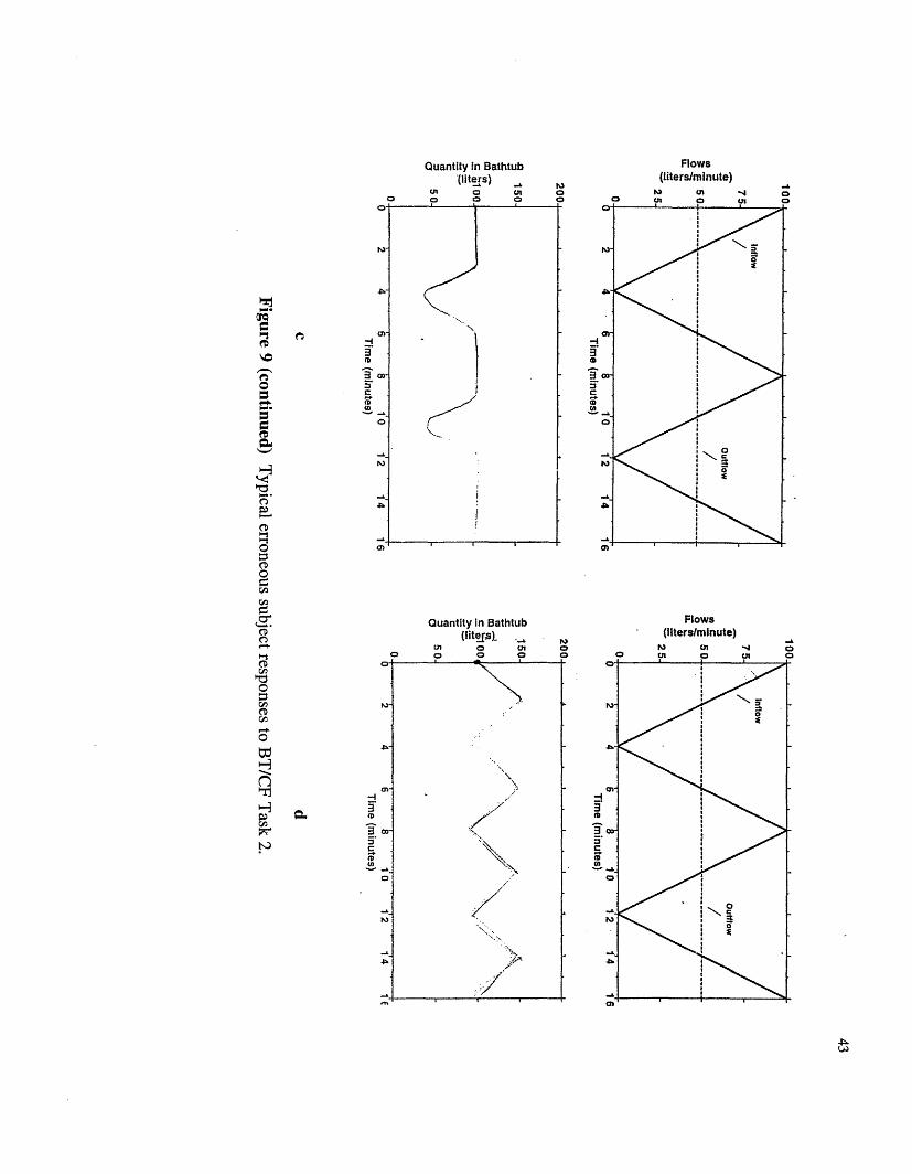
Quantity In Bathtub Flows(liters) (liters/minute)

CQW.cm

3

_f 3

E;

CD

©CD

e. Quanttyin Bathtub Flows

C'D (litgs) _ ,, (liters/minute)0 (IitffS)U, Ul 0

(D o-

c, WCDciO0

-T3

c,W _

n

o

_ o 0 $ CA o ,-.srr d c

IAI

": 'AI;

.--43

9X3X, IM

-- 1 1

.

C_ CD

-

v.

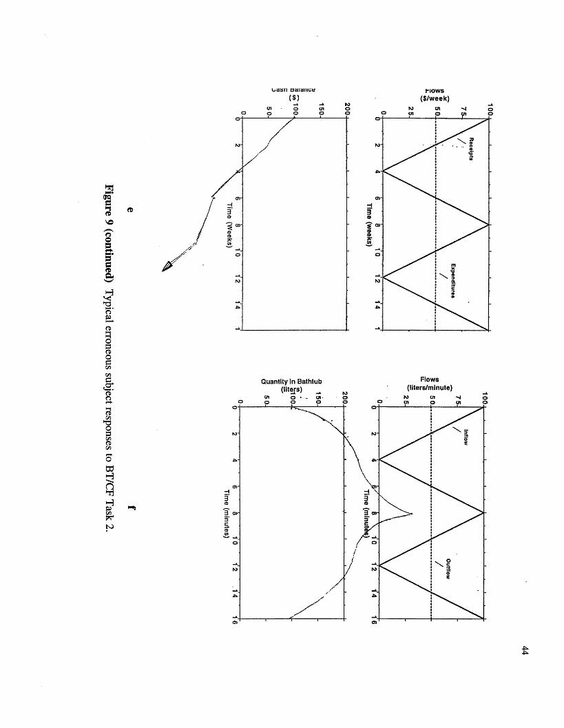
lOWS

($/week)

3-I

A

Quantity in Bathtub Flows(liters) , (liters/minute)

0

0

Icm

"1

0CoA

Co

co0

CDC

r-

CrA

Cr -

5.E...EL

adslI itllifc;!

Quantity in Bathtub(liters}

* **\ -c

\' .Ž*

Flows(liters/minute)

Flows(liters/minute)

d3S.

C0j

EtoA

0I

C,,la

0

0c$

CD0

Toci,

t')

0

AL

..._5

-43

C:D

-4·

3

S'0af

I\ NZ0 J

-111-

(000o o

CA_,(O

U'

00

Units/Week

0o

.. . . .

to

.

oo0

Units/Week

. . , .,,.,... P.... ....'

Ur

_ S , . ,

Units

o Io

0

0ee

Ur

o -

0a

R0n(D

I.....O

CD0rr.

CDo0

.

CDo

CDC)

-tcn

CD

Units

Ia

O' B w w w w - - - -i - - -

IDI:1

-Z

om

. . . . . . .

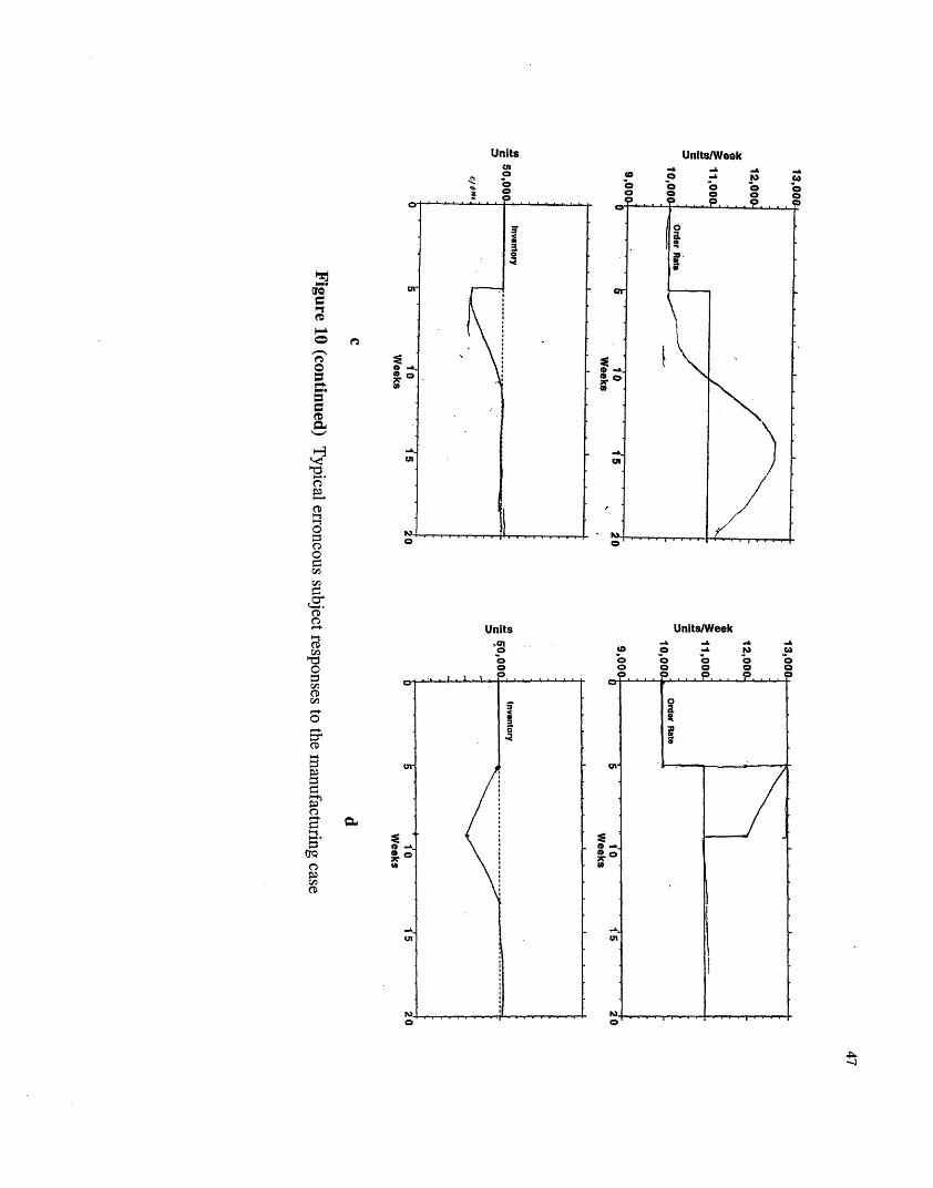
Units Units/Week

OI

H

b.Cm

C

'~1

M

oc 0 la~~~·- 1~~V..-t

S,0

M

C

or,

0

* jCA

In

4, , -. -A

0 a - a a=C _O _C C. . .P . . . . ..

0

a0

\

. . .D c. . .o

CD

1+ |Units Units/WeekCD M &n - . -cn o^ to o _C p 0

,it -0 0 a 0 0 00

cnCD

Cn5'

0

CD

0 0 0 a_~ _ _

o,0 -.~0

CI'

M.

. . ,. -A

o0a0I0

41.

_ _

F. - -

I-!

5

_

0-

cn-

. . . .

-- rc

I .

II

I . . � . . . .w

ur

0

Units/Week

Units/Week

p p -& 14 (0

a 0 o o 0a 0 0 00s D . . D . .'P. . . .

aio

) r

Unitstn

o00O

1r

M1

o.

' _(A1

-0

.ap* p

o

o

0,

-t

0

0.-

00o

e:0s0

CDcn

wp

0tOrQ 'A

o

00

I I . .

. . r . & v v w s l· - -l; - r

-:e IIIfi t

, X S

. I

I

I

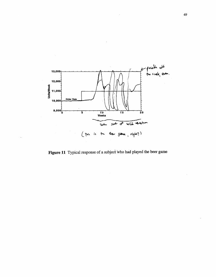
49

-A _IL& dL4

Weeks

go" S14- &e w;1c air~*

Co ;v is t" Z g , KlLvl

Figure 11 Typical response of a subject who had played the beer game

S0

a

'E0

it, S 6 V

O

Ave -I I X2 p BG -BG X2

1 Production must start in equilibriumwith orders.

2 Production must be constant prior totime 5 and indicate a lag of four weeks inthe response to the step increase inorders.

3 Production must overshoot orders toreplenish the inventory lost during theinitial period when orders exceedproduction. Production should return to(or fluctuate around) the equilibrium rateof 11,000 widgets/week (to keepinventory at or fluctuating around thedesired level)

4 Conservation of material: The areaenclosed by production and orders duringthe overshoot of production (whenproduction > orders) must equal the areaenclosed by orders less production (whenproduction < orders).

5 Inventory must initially decline (becauseproduction < orders).

0.53 0.72 0.33 33.8 0.001 0.57 0.47 2.3 0.13

0.44 0.59 0.29 20.3 0.001 0.46 0.41 0.6 0.43

0.44 0.63 0.23 36.5 0.001 0.53 0.30 11.5 0.001

0.11 0.12 0.10 0.06 0.80 0.16 0.05 2.9 0.09

0.68 NA 0.68 NA NA 0.77 0.55 6.1 0.01

6 Inventory must recover after droppinginitially.

7 Inventory must be consistent with thetrajectory of production and orders.

Mean for all items

0.56 NA 0.56 NA NA 0.66 0.43 5.6 0.02

0.10 NA 0.10 NA NA 0.14 0.06 1.6 0.21

0.41 0.50 0.32 t=5.11

0.0001 0.46 0.33

Table 5 Performance on the Manufacturing Case

I = Inventory graph; -I = No Inventory graph. BG = Beer Game experience; -BG = no BeerGame experience. Points 4-7 do not apply to the -I treatment. The X2 statistic tests thehypothesis that performance on the two treatment conditions ( I vs. -I and BG vs. -BG) is thesame.

Criterion

50

P

0.001t3=

3.35

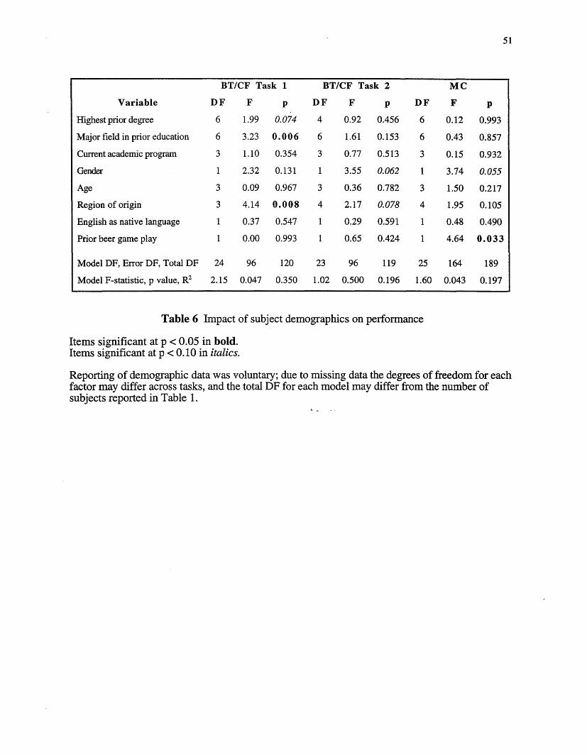
51

Table 6 Impact of subject demographics on performance

Items significant at p < 0.05 in bold.Items significant at p < 0.10 in italics.

Reporting of demographic data was voluntary; due to missing data the degrees of freedom for eachfactor may differ across tasks, and the total DF for each model may differ from the number ofsubjects reported in Table 1.

BT/CF Task 1 BT/CF Task 2 MC

Variable DF F p DF F p DF F p

Highest prior degree 6 1.99 0.074 4 0.92 0.456 6 0.12 0.993

Major field in prior education 6 3.23 0.006 6 1.61 0.153 6 0.43 0.857

Current academic program 3 1.10 0.354 3 0.77 0.513 3 0.15 0.932

Gender 1 2.32 0.131 1 3.55 0.062 1 3.74 0.055

Age 3 0.09 0.967 3 0.36 0.782 3 1.50 0.217

Region of origin 3 4.14 0.008 4 2.17 0.078 4 1.95 0.105

English as native language 1 0.37 0.547 1 0.29 0.591 1 0.48 0.490

Prior beer game play 1 0.00 0.993 1 0.65 0.424 1 4.64 0.033

Model DF, Error DF, Total DF 24 96 120 23 96 119 25 164 189

Model F-statistic, p value, R2 2.15 0.047 0.350 1.02 0.500 0.196 1.60 0.043 0.197