initiation a la v eri cation basics of veri cation
TRANSCRIPT
1/131
Initiation a la verificationBasics of Verification
https://wikimpri.dptinfo.ens-cachan.fr/doku.php?id=cours:c-1-22
Paul Gastin
http://www.lsv.fr/~gastin/
MPRI – M12020 – 2021

2/131

2/131
Outline
1 Introduction
Models
Temporal Specifications
Satisfiability and Model Checking
More on Temporal Specifications
3/131
Need for formal verification methods
Critical systemsI Transport
I Energy
I Medicine
I Communication
I Finance
I Embedded systems
I . . .

4/131
Disastrous software bugs
https://en.wikipedia.org/wiki/List_of_software_bugs
Mariner 1 probe, 1962
See http://en.wikipedia.org/wiki/Mariner_1
I Destroyed 293 seconds after launch
I Missing hyphen in the data or program? No!
I Overbar missing in the mathematicalspecification:
Rn: nth smoothed value of the time derivativeof a radius.Without the smoothing function indicated bythe bar, the program treated normal minorvariations of velocity as if they were serious,causing spurious corrections that sent therocket off course.

5/131
Disastrous software bugsAriane 5 flight 501, 1996
See http://en.wikipedia.org/wiki/Ariane_5_Flight_501
I Destroyed 37 seconds after launch (cost: 370 millionsdollars).
I data conversion from a 64-bit floating point to 16-bitsigned integer value caused a hardware exception(arithmetic overflow).
I Efficiency considerations had led to the disabling of thesoftware handler (in Ada code) for this error trap.
I The fault occured in the inertial reference system of Ariane5. The software from Ariane 4 was re-used for Ariane 5without re-testing.
I On the basis of those calculations the main computercommanded the booster nozzles, and somewhat later themain engine nozzle also, to make a large correction for anattitude deviation that had not occurred.
I The error occurred in a realignment function which was notuseful for Ariane 5.
6/131
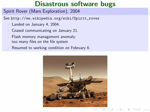
Disastrous software bugsSpirit Rover (Mars Exploration), 2004
See http://en.wikipedia.org/wiki/Spirit_rover
I Landed on January 4, 2004.
I Ceased communicating on January 21.
I Flash memory management anomaly:too many files on the file system
I Resumed to working condition on February 6.
7/131
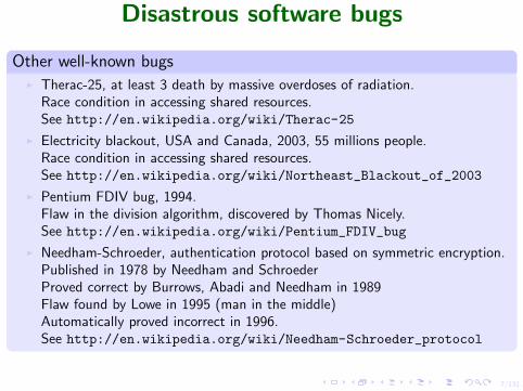
Disastrous software bugs
Other well-known bugsI Therac-25, at least 3 death by massive overdoses of radiation.
Race condition in accessing shared resources.See http://en.wikipedia.org/wiki/Therac-25
I Electricity blackout, USA and Canada, 2003, 55 millions people.Race condition in accessing shared resources.See http://en.wikipedia.org/wiki/Northeast_Blackout_of_2003
I Pentium FDIV bug, 1994.Flaw in the division algorithm, discovered by Thomas Nicely.See http://en.wikipedia.org/wiki/Pentium_FDIV_bug
I Needham-Schroeder, authentication protocol based on symmetric encryption.Published in 1978 by Needham and SchroederProved correct by Burrows, Abadi and Needham in 1989Flaw found by Lowe in 1995 (man in the middle)Automatically proved incorrect in 1996.See http://en.wikipedia.org/wiki/Needham-Schroeder_protocol
8/131
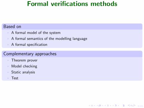
Formal verifications methods
Based onI A formal model of the system
I A formal semantics of the modelling language
I A formal specification
Complementary approachesI Theorem prover
I Model checking
I Static analysis
I Test

9/131
Model Checking
I Purpose 1: automatically finding software or hardware bugs.
I Purpose 2: prove correctness of abstract models.
I Should be applied during design.
I Real systems can be analysed with abstractions.
E.M. Clarke E.A. Emerson J. Sifakis
Prix Turing 2007.

10/131
Model Checking3 steps
I Constructing the model M (transition systems)
I Formalizing the specification ϕ (temporal logics)
I Checking whether M |= ϕ (algorithmics)
Main difficultiesI Size of models (combinatorial explosion)
I Expressivity of models or logics
I Decidability and complexity of the model-checking problem
I Efficiency of tools
ChallengesI Extend models and algorithms to cope with more systems.
Infinite systems, parameterized systems, probabilistic systems, concurrentsystems, timed systems, hybrid systems, . . . See Modules 2.8 & 2.9
I Scale current tools to cope with real-size systems.Needs for modularity, abstractions, symmetries, . . .

11/131
References[1] Christel Baier and Joost-Pieter Katoen.
Principles of Model Checking.MIT Press, 2008.
[2] B. Berard, M. Bidoit, A. Finkel, F. Laroussinie, A. Petit, L. Petrucci,Ph. Schnoebelen.Systems and Software Verification. Model-Checking Techniques and Tools.Springer, 2001.
[3] E.M. Clarke, O. Grumberg, D.A. Peled.Model Checking.MIT Press, 1999.
[4] Z. Manna and A. Pnueli.The Temporal Logic of Reactive and Concurrent Systems: Specification.Springer, 1991.
[5] Z. Manna and A. Pnueli.Temporal Verification of Reactive Systems: Safety.Springer, 1995.
[6] Ph. Schnoebelen.The Complexity of Temporal Logic Model Checking.In AiML’02, 393–436. King’s College Publication, 2003.

12/131
Outline
Introduction
2 Models
Transition Systems
. . . with Variables
Concurrent Systems
Synchronization and Communication
Temporal Specifications
Satisfiability and Model Checking
More on Temporal Specifications

14/131
Model and abstractionsExample: Golden face
Each coin has a golden face and a silver face.At each step, we may flip simultaneously the 3 coins of a line, column or diagonal.Is it possible to have all coins showing its golden face ?If yes, what is the smallest number of steps.
Model = Transition system
I States: configurations of the board: 29 = 512 states
I Transitions: flipping a line/column/diagonal
I Problem: reachability
Abstraction 1: number of golden faces in a configuration.Abstraction 2: parity of the number of golden faces in the corners.

15/131
Model and Specification
Example: Man, Wolf, Goat, Cabbage
Model = Transition systemI State = who is on which side of the river
I Transition = crossing the river, M alone or with one of W,G,C
I SpecificationSafety: Never leave WG or GC aloneLiveness: Take everyone to the other side of the river.

17/131
Transition system or Kripke structure
Definition: TS M = (S,Σ, T, I,AP, `)
I S: set of states (finite or infinite)
I Σ: set of actions
I T ⊆ S × Σ× S: set of transitions
I I ⊆ S: set of initial states
I AP: set of atomic propositions
I ` : S → 2AP: labelling function.
Every discrete system may be described with a TS.
Example: Digicode ABA
1 2 3 4
OPEN
A B A
B,C A
C
B,C

18/131
Description Languages
Pb: How can we easily describe big systems?
Description Languages (high level)I Programming languages
I Boolean circuits
I Modular description, e.g., parallel compositionsproblems: concurrency, synchronization, communication, atomicity, fairness, ...
I Petri nets (intermediate level)
I Transition systems (intermediate level)with variables, stacks, channels, ...synchronized products
I Logical formulae (low level)
Operational semantics
High level descriptions are translated (compiled) to low level (infinite) TS.
20/131
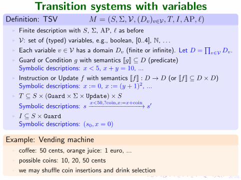
Transition systems with variablesDefinition: TSV M = (S,Σ,V , (Dv)v∈V , T, I,AP, `)
I Finite description with S, Σ, AP, ` as before
I V: set of (typed) variables, e.g., boolean, [0..4], N, . . .
I Each variable v ∈ V has a domain Dv (finite or infinite). Let D =∏v∈V Dv.
I Guard or Condition g with semantics [[g]] ⊆ D (predicate)Symbolic descriptions: x < 5, x+ y = 10, ...
I Instruction or Update f with semantics [[f ]] : D → D (or [[f ]] ⊆ D ×D)Symbolic descriptions: x := 0, x := (y + 1)2, ...
I T ⊆ S × (Guard× Σ× Update)× SSymbolic descriptions: s
x<50,?coin,x:=x+coin−−−−−−−−−−−−−−→ s′
I I ⊆ S × Guard
Symbolic descriptions: (s0, x = 0)
Example: Vending machineI coffee: 50 cents, orange juice: 1 euro, ...
I possible coins: 10, 20, 50 cents
I we may shuffle coin insertions and drink selection

21/131
Transition systems with variablesSemantics: low level TS
I S′ = S ×DI I ′ = {(s, ν) | ∃(s, g) ∈ I with ν |= g}I Transitions: T ′ ⊆ (S ×D)× Σ× (S ×D)
sg,a,f−−−→ s′ ∧ ν |= g
(s, ν)a−→ (s′, f(ν))
SOS: Structural Operational Semantics
I AP′: we may use atomic propositions in AP or guards such as x > 0.
Programs = Kripke structures with variablesI Program counter = states
I Instructions = transitions
I Variables = variables
Example: GCD

22/131
TS with variables . . .
Example: Digicode
1cpt = 0
2 3 4
OPEN
A B A
cpt < nB,Ccpt++
cpt < nAcpt++
cpt < nCcpt++
cpt < nB,Ccpt++
5
ERROR
cpt = nB,Ccpt++
cpt = nA,Ccpt++
cpt = nB,Ccpt++

24/131
Only variablesThe state is nothing but a special variable: s ∈ V with domain Ds = S.
Definition: TSV M = (V , (Dv)v∈V , T, I,AP, `)
I D =∏v∈V Dv,
I I ⊆ D, T ⊆ D ×D
Symbolic representations with logic formulaeI I given by a formula ψ(ν)
I T given by a formula ϕ(ν, ν′)ν: values before the transitionν′: values after the transition
I Often we use boolean variables only: Dv = {0, 1}I Concise descriptions of boolean formulae with Binary Decision Diagrams.
Example: Boolean circuit: modulo 8 counter
b′0 = ¬b0b′1 = b0 ⊕ b1b′2 = (b0 ∧ b1)⊕ b2
27/131
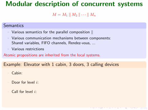
Modular description of concurrent systems
M = M1 ‖M2 ‖ · · · ‖Mn
SemanticsI Various semantics for the parallel composition ‖I Various communication mechanisms between components:
Shared variables, FIFO channels, Rendez-vous, ...
I Various restrictions
Atomic propositions are inherited from the local systems.
Example: Elevator with 1 cabin, 3 doors, 3 calling devices
I Cabin:
0 1 2
I Door for level i:
Closed Opened
I Call for level i:
False True
The actual system is a synchronized product of all these automata.It consists of (at most) 3× 23 × 23 = 192 states.
28/131
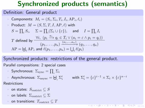
Synchronized products (semantics)Definition: General product
I Components: Mi = (Si,Σi, Ti, Ii,APi, `i)
I Product: M = (S,Σ, T, I,AP, `) with
S =∏i Si, Σ =
∏i(Σi ∪ {ε}), and I =
∏i Ii
T defined by∀i, (pi
ai−→ qi ∈ Ti ∨ (ai = ε ∧ pi = qi))
(p1, . . . , pn)(a1,...,an)−−−−−−→ (q1, . . . , qn)
AP =⊎i APi and `(p1, . . . , pn) =
⋃i `(pi)
Synchronized products: restrictions of the general product.
Parallel compositions: 2 special cases
I Synchronous: Σsync =∏
iΣi
I Asynchronous: Σasync =⊎
iΣ′i with Σ′i = {ε}i−1 × Σi × {ε}n−i
Restrictions
I on states: Srestrict ⊆ SI on labels: Σrestrict ⊆ Σ
I on transitions: Trestrict ⊆ T

32/131
Shared variables
Definition: Asynchronous product + shared variables
s = (s1, . . . , sn) denotes a tuple of statesν ∈ D =
∏v∈V Dv is a valuation of variables.
Semantics (SOS)ν |= g ∧ si
g,a,f−−−→ s′i ∧ s′j = sj for j 6= i
(s, ν)a−→ (s′, f(ν))
Example: Mutual exclusion for 2 processes satisfyingI Safety: never simultaneously in critical section (CS).
I Liveness: if a process wants to enter its CS, it eventually does.
I Fairness: if process 1 wants to enter its CS, then process 2 will enter its CS atmost once before process 1 does.
using shared variables but without further restrictions: the atomicity is
I testing or reading or writing a single variable at a time
I no test-and-set: {x = 0;x := 1}
33/131
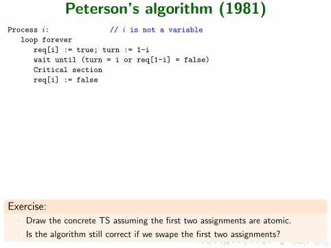
Peterson’s algorithm (1981)Process i: // i is not a variable
loop forever
req[i] := true; turn := 1-i
wait until (turn = i or req[1-i] = false)
Critical section
req[i] := false
1 2
Waiti
3
Waiti
4
CSi
req[i]:=true
turn:=1-i
turn=i?
req[1-i]=false?
req[i]:=false
elseuse
idle
Exercise:I Draw the concrete TS assuming the first two assignments are atomic.
I Is the algorithm still correct if we swape the first two assignments?
34/131
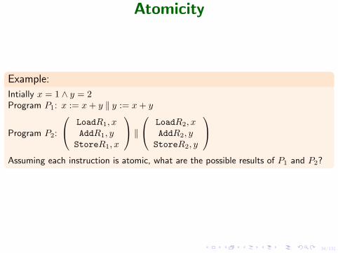
Atomicity
Example:
Intially x = 1 ∧ y = 2Program P1: x := x+ y ‖ y := x+ y
Program P2:
LoadR1, xAddR1, y
StoreR1, x
‖ LoadR2, x
AddR2, yStoreR2, y
Assuming each instruction is atomic, what are the possible results of P1 and P2?

35/131
Atomicity
Definition: Atomic statements: atomic(ES)
Elementary statements (no loops, no communications, no synchronizations)
ES ::= skip | await c | x := e | ES ; ES | ES 2 ES
| when c do ES | if c then ES else ES
Atomic statements: if the ES can be fully executed then it is executed in one step.
(s, ν) ES−−−→∗ (s′, ν′)
(s, ν)atomic(ES)−−−−−−−→ (s′, ν′)
Example: Atomic statementsI atomic(x = 0;x := 1) (Test and set)
I atomic(y := y − 1; await(y = 0); y := 1) is equivalent to await(y = 1)
36/131
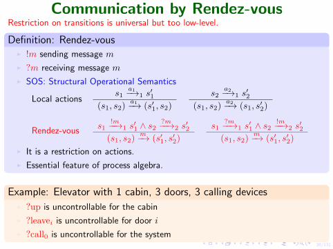
Communication by Rendez-vousRestriction on transitions is universal but too low-level.
Definition: Rendez-vousI !m sending message m
I ?m receiving message m
I SOS: Structural Operational Semantics
Local actionss1
a1−→1 s′1
(s1, s2)a1−→ (s′1, s2)
s2a2−→1 s
′2
(s1, s2)a2−→ (s1, s
′2)
Rendez-vouss1
!m−−→1 s′1 ∧ s2
?m−−→2 s′2
(s1, s2)m−→ (s′1, s
′2)
s1?m−−→1 s
′1 ∧ s2
!m−−→2 s′2
(s1, s2)m−→ (s′1, s
′2)
I It is a restriction on actions.
I Essential feature of process algebra.
Example: Elevator with 1 cabin, 3 doors, 3 calling devicesI ?up is uncontrollable for the cabin
I ?leavei is uncontrollable for door i
I ?call0 is uncontrollable for the system

38/131
Channels
Example: Leader election
We have n processes on a directed ring, each having a unique id ∈ {1, . . . , n}.
send(id)
loop forever
receive(x)
if (x = id) then STOP fi
if (x > id) then send(x)

39/131
Channels
Definition: ChannelsI Declaration:
c : channel [k] of bool size kc : channel [∞] of int unboundedc : channel [0] of colors Rendez-vous
I Primitives:empty(c)c!e add the value of expression e to channel cc?x read a value from c and assign it to variable x
I Domain: Let Dm be the domain for a single message.
Dc = D≤km size kDc = D∗m unboundedDc = {ε} Rendez-vous
I Politics: FIFO, LIFO, BAG, . . .
40/131
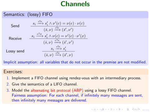
Channels
Semantics: (lossy) FIFO
Sendsi
c!e−−→ s′i ∧ ν′(c) = ν(e) · ν(c)
(s, ν)c!e−−→ (s′, ν′)
Receivesi
c?x−−→ s′i ∧ ν(c) = ν′(c) · ν′(x)
(s, ν)c?e−−→ (s′, ν′)
Lossy sendsi
c!e−−→ s′i
(s, ν)c!e−−→ (s′, ν)
Implicit assumption: all variables that do not occur in the premise are not modified.
Exercises:1. Implement a FIFO channel using rendez-vous with an intermediary process.
2. Give the semantics of a LIFO channel.
3. Model the alternating bit protocol (ABP) using a lossy FIFO channel.Fairness assumption: For each channel, if infinitely many messages are sent,then infinitely many messages are delivered.

41/131
High-level descriptions
SummaryI Sequential program = transition system with variables
I Concurrent program with shared variables
I Concurrent program with Rendez-vous
I Concurrent program with FIFO communication
I Petri net
I . . .

42/131
Models: expressivity versus decidability
Remark: (Un)decidabilityI Automata with 2 integer variables = Turing powerful
Restriction to variables taking values in finite sets
I Asynchronous communication: unbounded fifo channels = Turing powerfulRestriction to bounded channels or lossy channels
Remark: Some infinite state models are decidableI Petri nets. Several unbounded integer variables but no zero-test.
I Pushdown automata. Model for recursive procedure calls.
I Timed automata.
I . . .

43/131
Outline
Introduction
Models
3 Temporal Specifications
General Definitions
(Linear) Temporal Specifications
Branching Temporal Specifications
CTL∗
CTL
Satisfiability and Model Checking
More on Temporal Specifications

45/131
Static and dynamic properties
Example: Static properties
Mutual exclusion
¬(Crit1 ∧ Crit2) or ∀t,¬(Crit1(t) ∧ Crit2(t))
Safety properties are often static.
They can be reduced to reachability.
Example: Dynamic properties
Every elevator request should be eventually granted.
∧i
∀t, (Calli(t) −→ ∃t′ ≥ t, (atLeveli(t′) ∧ openDoori(t
′)))
The elevator should not cross a level for which a call is pending without stopping.
∧i
∀t∀t′, (Calli(t) ∧ t ≤ t′ ∧ atLeveli(t′)) −→
∃t ≤ t′′ ≤ t′, (atLeveli(t′′) ∧ openDoori(t
′′)))

46/131
Temporal StructuresDefinition: Flows of time
A flow of time is a strict order (T, <) where T is the nonempty set of time pointsand < is an irreflexive transitive relation on T.
Example: Flows of timeI ({0, . . . , n}, <): Finite runs of sequential systems.
I (N, <): Infinite runs of sequential systems.
I (R, <): runs of real-time sequential systems.
I Trees: Finite or infinite run-trees of sequential systems.
I Mazurkiewicz traces: runs of distributed systems (rendez-vous).
I Message sequence charts: runs of distributed systems (FIFO).
I and also (Z, <) or (Q, <) or (ω2, <), . . .
Definition: Temporal Structures
Let AP be a set of atoms (atomic propositions) and let C be a class of time flows.A temporal structure over (C,AP) is a triple (T, <, λ) where (T, <) is a time flowin C and λ : T→ 2AP labels time points with atomic propositions.The temporal structure (T, <, λ) is also denoted (T, <, h) where h : AP → 2T
assigns time points to atomic propositions: h(p) = {t ∈ T | p ∈ λ(t)} for p ∈ AP.

47/131
Linear behaviors and specifications
Let M = (S, T, I,AP, `) be a Kripke structure (we omit actions: T ⊆ S × S).
Definition: Runs as temporal structures
An infinite run σ = s0s1s2 · · · of M with (si, si+1) ∈ T for all i ≥ 0 defines a lineartemporal structure `(σ) = (N, <, λ) where λ(i) = `(si) for i ∈ N.
Such a temporal structure can be seen as an infinite word over Σ = 2AP:`(σ) = `(s0)`(s1)`(s2) · · · ∈ Σω
Linear specifications only depend on runs.
Example: The printer manager is starvation free.
On each run, whenever some process requests the printer, it eventually gets it.
Remark:Two Kripke structures having the same linear temporal structures satisfy the samelinear specifications.
48/131
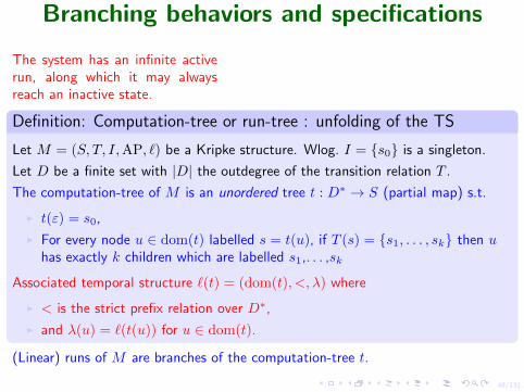
Branching behaviors and specifications
The system has an infinite activerun, along which it may alwaysreach an inactive state.
1
Active
2 3
Active
Definition: Computation-tree or run-tree : unfolding of the TS
Let M = (S, T, I,AP, `) be a Kripke structure. Wlog. I = {s0} is a singleton.
Let D be a finite set with |D| the outdegree of the transition relation T .
The computation-tree of M is an unordered tree t : D∗ → S (partial map) s.t.
I t(ε) = s0,
I For every node u ∈ dom(t) labelled s = t(u), if T (s) = {s1, . . . , sk} then uhas exactly k children which are labelled s1,. . . ,sk
Associated temporal structure `(t) = (dom(t), <, λ) where
I < is the strict prefix relation over D∗,
I and λ(u) = `(t(u)) for u ∈ dom(t).
(Linear) runs of M are branches of the computation-tree t.

49/131
First-order SpecificationsDefinition: Syntax of FO(AP, <)
Let Var = {x, y, . . .} be first-order variables.
ϕ ::= ⊥ | p(x) | x = y | x < y | ¬ϕ | ϕ ∨ ϕ | ∃xϕ
where p ∈ AP.
Definition: Semantics of FO(AP, <)
Let w = (T, <, λ) be a temporal structure over AP.Let ν : Var→ T be an assignment of first-order variables to time points.
w, ν |= p(x) if p ∈ λ(ν(x))
w, ν |= x = y if ν(x) = ν(y)
w, ν |= x < y if ν(x) < ν(y)
w, ν |= ∃xϕ if w, ν[x 7→ t] |= ϕ for some t ∈ T
where ν[x 7→ t] maps x to t and y 6= x to ν(y).
Previous specifications can be written in FO(<) (except the branching one).
50/131
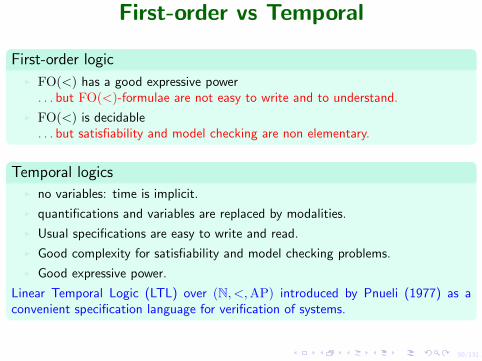
First-order vs Temporal
First-order logicI FO(<) has a good expressive power
. . . but FO(<)-formulae are not easy to write and to understand.
I FO(<) is decidable. . . but satisfiability and model checking are non elementary.
Temporal logicsI no variables: time is implicit.
I quantifications and variables are replaced by modalities.
I Usual specifications are easy to write and read.
I Good complexity for satisfiability and model checking problems.
I Good expressive power.
Linear Temporal Logic (LTL) over (N, <,AP) introduced by Pnueli (1977) as aconvenient specification language for verification of systems.
52/131
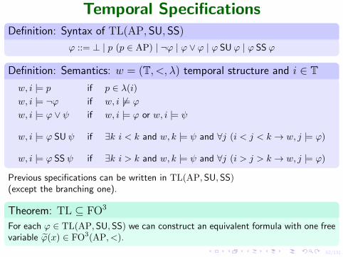
Temporal SpecificationsDefinition: Syntax of TL(AP, SU, SS)
ϕ ::= ⊥ | p (p ∈ AP) | ¬ϕ | ϕ ∨ ϕ | ϕ SU ϕ | ϕ SS ϕ
Definition: Semantics: w = (T, <, λ) temporal structure and i ∈ Tw, i |= p if p ∈ λ(i)
w, i |= ¬ϕ if w, i 6|= ϕ
w, i |= ϕ ∨ ψ if w, i |= ϕ or w, i |= ψ
w, i |= ϕ SU ψ if ∃k i < k and w, k |= ψ and ∀j (i < j < k → w, j |= ϕ)
w, i |= ϕ SS ψ if ∃k i > k and w, k |= ψ and ∀j (i > j > k → w, j |= ϕ)
Previous specifications can be written in TL(AP,SU,SS)(except the branching one).
Theorem: TL ⊆ FO3
For each ϕ ∈ TL(AP,SU,SS) we can construct an equivalent formula with one freevariable ϕ(x) ∈ FO3(AP, <).

53/131
Temporal SpecificationsDefinition: non-strict versions of until and since
ϕ U ψdef= ψ ∨ (ϕ ∧ ϕ SU ψ) ϕ S ψ
def= ψ ∨ (ϕ ∧ ϕ SS ψ)
w, i |= ϕ U ψ if ∃k i ≤ k and w, k |= ψ and ∀j (i ≤ j < k → w, j |= ϕ)
w, i |= ϕ S ψ if ∃k i ≥ k and w, k |= ψ and ∀j (i ≥ j > k → w, j |= ϕ)
Definition: Derived modalities
Xϕdef= ⊥ SU ϕ Next Yϕ
def= ⊥ SS ϕ Yesterday
w, i |= Xϕ if ∃k i < k and w, k |= ϕ and ¬∃j (i < j < k)
w, i |= Yϕ if ∃k i > k and w, k |= ϕ and ¬∃j (i > j > k)
SFϕdef= > SU ϕ SPϕ
def= > SS ϕ
Fϕdef= > U ϕ Pϕ
def= > S ϕ
Gϕdef= ¬F¬ϕ Hϕ
def= ¬P¬ϕ
ϕW ψdef= (Gϕ) ∨ (ϕ U ψ) Weak Until
ϕ R ψdef= (Gψ) ∨ (ψ U (ϕ ∧ ψ)) Release

55/131
Temporal Specifications
Example: Specifications on the time flow (N, <)I Safety: G good
I MutEx: ¬F(crit1 ∧ crit2)
I Liveness: G F active
I Response: G(request→ F grant)
I Response’: G(request→ (¬request SU grant))
I Release: reset R alarm
I Strong fairness: (G F request)→ (G F grant)
I Weak fairness: (F G request)→ (G F grant)
I Stability: G¬p ∨ (¬p U G p)

56/131
Discrete linear time flowsDefinition: discrete linear time flows (T, <)
A linear time flow is discrete if SF> → X> and SP> → Y> are valid formulae.
(N, <) and (Z, <) are discrete.
(Q, <) and (R, <) are not discrete.
Exercise: For discrete linear time flows (T, <)
ϕ SU ψ ≡ X(ϕ U ψ) ¬Xϕ ≡ ¬X> ∨ X¬ϕϕ SS ψ ≡ Y(ϕ S ψ) ¬Yϕ ≡ ¬Y> ∨ Y¬ϕ
¬(ϕ U ψ) ≡ (G¬ψ) ∨ (¬ψ U (¬ϕ ∧ ¬ψ))≡ ¬ψ W (¬ϕ ∧ ¬ψ)≡ ¬ϕ R ¬ψ
Remark: Dense time flow T = Q or T = R¬(ϕ U ψ) does not imply ¬ϕ R ¬ψ.
For instance, w = (T, <, `) with T = {0} ∪ { 1n | n ∈ N} with `(0) = {p},
`( 12n ) = {p} and `( 1
2n+1 ) = {q}. Then, w, 0 |= ¬(p U q) and w, 0 6|= ¬p R ¬q.

57/131
Model checking for linear behaviors
Definition: Model checking problem
Input: A Kripke structure M = (S, T, I,AP, `)A formula ϕ ∈ LTL(AP,SU,SS)
Question: Does M |= ϕ ?
I Universal MC: M |=∀ ϕ if `(σ), 0 |= ϕ for all initial infinite runs σ of M .
I Existential MC: M |=∃ ϕ if `(σ), 0 |= ϕ for some initial infinite run σ of M .
M |=∀ ϕ iff M 6|=∃ ¬ϕ
Theorem [11, Sistla, Clarke 85], [10, Lichtenstein & Pnueli 85]
The Model checking problem for LTL is PSPACE-complete. Proof later
59/131
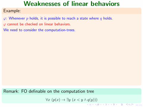
Weaknesses of linear behaviorsExample:
ϕ: Whenever p holds, it is possible to reach a state where q holds.
ϕ cannot be checked on linear behaviors.
We need to consider the computation-trees.
Consider the two models:
M1: 1
p, q
2
p3
q
4
and M2: 1
p, q2
p
2’
p
3
q
4
M1 |= ϕ but M2 6|= ϕ
M1 and M2 have the same linear behaviors.
Remark: FO definable on the computation tree
∀x (p(x)→ ∃y (x < y ∧ q(y)))
60/131
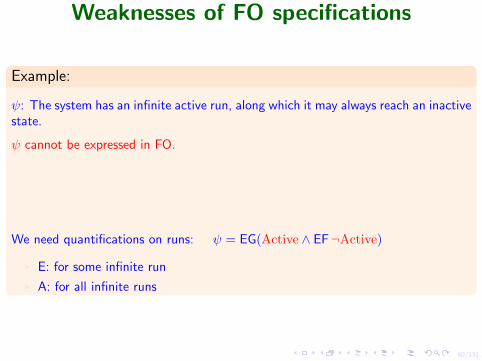
Weaknesses of FO specifications
Example:
ψ: The system has an infinite active run, along which it may always reach an inactivestate.
ψ cannot be expressed in FO.
1
Active
2 3
Active
We need quantifications on runs: ψ = EG(Active ∧ EF¬Active)
I E: for some infinite run
I A: for all infinite runs

61/131
MSO Specifications
Definition: Syntax of MSO(AP, <)
ϕ ::= ⊥ | p(x) | x = y | x < y | x ∈ X | ¬ϕ | ϕ ∨ ϕ | ∃xϕ | ∃X ϕ
where p ∈ AP, x, y are first-order variables and X is a second-order variable.
Definition: Semantics of MSO(AP, <)
Let w = (T, <, λ) be a temporal structure over AP.An assignment ν maps first-order variables to time points in Tand second-order variables to sets of time points.
The semantics of first-order constructs is unchanged.
w, ν |= x ∈ X if ν(x) ∈ ν(X)
w, ν |= ∃X ϕ if w, ν[X 7→ T ] |= ϕ for some T ⊆ T
where ν[X 7→ T ] maps X to T and keeps unchanged the other assignments.
63/131
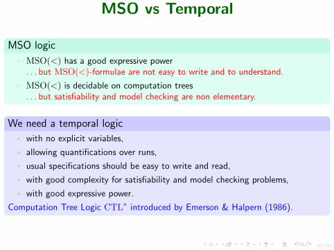
MSO vs Temporal
MSO logicI MSO(<) has a good expressive power
. . . but MSO(<)-formulae are not easy to write and to understand.
I MSO(<) is decidable on computation trees. . . but satisfiability and model checking are non elementary.
We need a temporal logicI with no explicit variables,
I allowing quantifications over runs,
I usual specifications should be easy to write and read,
I with good complexity for satisfiability and model checking problems,
I with good expressive power.
Computation Tree Logic CTL∗ introduced by Emerson & Halpern (1986).
65/131
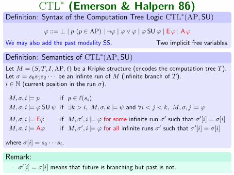
CTL∗ (Emerson & Halpern 86)Definition: Syntax of the Computation Tree Logic CTL∗(AP, SU)
ϕ ::= ⊥ | p (p ∈ AP) | ¬ϕ | ϕ ∨ ϕ | ϕ SU ϕ | Eϕ | Aϕ
We may also add the past modality SS. Two implicit free variables.
Definition: Semantics of CTL∗(AP, SU)
Let M = (S, T, I,AP, `) be a Kripke structure (encodes the computation tree T ).Let σ = s0s1s2 · · · be an infinte run of M (infinite branch of T ).i ∈ N (current position in the run σ).
M,σ, i |= p if p ∈ `(si)M,σ, i |= ϕ SU ψ if ∃k > i, M, σ, k |= ψ and ∀i < j < k, M, σ, j |= ϕ
M,σ, i |= Eϕ if M,σ′, i |= ϕ for some infinite run σ′ such that σ′[i] = σ[i]
M,σ, i |= Aϕ if M,σ′, i |= ϕ for all infinite runs σ′ such that σ′[i] = σ[i]
where σ[i] = s0 · · · si.
Remark:I σ′[i] = σ[i] means that future is branching but past is not.

66/131
CTL∗ (Emerson & Halpern 86)
Example: Some specificationsI EFϕ: ϕ is possible FO-definable on CT
I AGϕ: ϕ is an invariant FO-definable on CT
I AFϕ: ϕ is unavoidable not FO-definable on CT
I EGϕ: ϕ holds globally along some path not FO-definable on CT
Remark: Some equivalencesI Aϕ ≡ ¬E¬ϕI E(ϕ ∨ ψ) ≡ Eϕ ∨ Eψ
I A(ϕ ∧ ψ) ≡ Aϕ ∧ Aψ
Theorem: CTL∗ ⊆ MSO
For each ϕ ∈ CTL∗(AP,SU) we can construct an equivalent formula with two freevariables ϕ(X,x) ∈ MSO(AP, <).For all computation tree T , infinite branch B of T and position i in B, we have
T,B, i |= ϕ iff T,X 7→ B, x 7→ i |= ϕ.
67/131
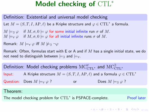
Model checking of CTL∗
Definition: Existential and universal model checking
Let M = (S, T, I,AP, `) be a Kripke structure and ϕ ∈ CTL∗ a formula.
M |=∃ ϕ if M,σ, 0 |= ϕ for some initial infinite run σ of M .M |=∀ ϕ if M,σ, 0 |= ϕ for all initial infinite runs σ of M .
Remark: M |=∀ ϕ iff M 6|=∃ ¬ϕ
Remark: Often, formulas start with E or A and if M has a single initial state, we donot need to distinguish between |=∃ and |=∀.
Definition: Model checking problems MC∀CTL∗ and MC∃CTL∗
Input: A Kripke structure M = (S, T, I,AP, `) and a formula ϕ ∈ CTL∗
Question: Does M |=∀ ϕ ? or Does M |=∃ ϕ ?
Theorem:
The model checking problem for CTL∗ is PSPACE-complete. Proof later

69/131
State formulae and path formulaeDefinition: State formulae
ϕ ∈ CTL∗ is a state formula if ∀M,σ, σ′, i, j such that σ(i) = σ′(j) we have
M,σ, i |= ϕ ⇐⇒ M,σ′, j |= ϕ
If ϕ is a state formula and M = (S, T, I,AP, `), define
M, s |= ϕ if M,σ, 0 |= ϕ for some infinite run σ of M with σ(0) = s
and [[ϕ]]M = {s ∈ S |M, s |= ϕ}
Example: State formulae
Atomic propositions are state formulae: [[p]] = {s ∈ S | p ∈ `(s)}State formulae are closed under boolean connectives.
[[¬ϕ]] = S \ [[ϕ]] [[ϕ1 ∨ ϕ2]] = [[ϕ1]] ∪ [[ϕ2]]
Formulae of the form Eϕ or Aϕ are state formulae, provided ϕ is future.
Remark: M |=∃ ϕ iff I ∩ [[Eϕ]] 6= ∅ M |=∀ ϕ iff I ⊆ [[Aϕ]]
Definition: Alternative syntax
State formulae ϕ ::= ⊥ | p (p ∈ AP) | ¬ϕ | ϕ ∨ ϕ | Eψ | AψPath formulae ψ ::= ϕ | ¬ψ | ψ ∨ ψ | ψ SU ψ
70/131
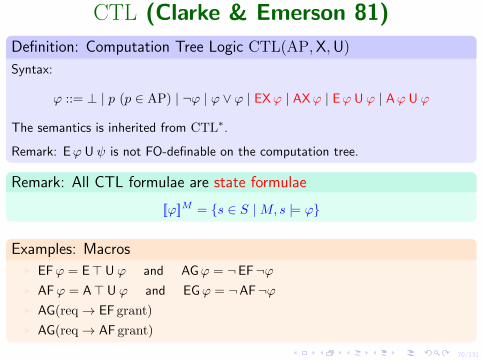
CTL (Clarke & Emerson 81)
Definition: Computation Tree Logic CTL(AP,X,U)
Syntax:
ϕ ::= ⊥ | p (p ∈ AP) | ¬ϕ | ϕ ∨ ϕ | EXϕ | AXϕ | Eϕ U ϕ | Aϕ U ϕ
The semantics is inherited from CTL∗.
Remark: Eϕ U ψ is not FO-definable on the computation tree.
Remark: All CTL formulae are state formulae
[[ϕ]]M = {s ∈ S |M, s |= ϕ}
Examples: MacrosI EFϕ = E> U ϕ and AGϕ = ¬EF¬ϕI AFϕ = A> U ϕ and EGϕ = ¬AF¬ϕI AG(req→ EF grant)
I AG(req→ AF grant)

71/131
CTL (Clarke & Emerson 81)
Definition: SemanticsAll CTL-formulae are state formulae. Hence, we have a simpler semantics.Let M = (S, T, I,AP, `) be a Kripke structure without deadlocks and let s ∈ S.
M, s |= p if p ∈ `(s)M, s |= EXϕ if ∃s→ s′ with M, s′ |= ϕ
M, s |= AXϕ if ∀s→ s′ we have M, s′ |= ϕ
M, s |= Eϕ U ψ if ∃s = s0 → s1 → s2 → · · · sk finite path, withM, sk |= ψ and M, sj |= ϕ for all 0 ≤ j < k
M, s |= Aϕ U ψ if ∀s = s0 → s1 → s2 → · · · infinite paths, ∃k ≥ 0 withM, sk |= ψ and M, sj |= ϕ for all 0 ≤ j < k
Theorem: CTL ⊆ MSO
For each ϕ ∈ CTL(AP,X,U) we can construct an equivalent formula with one freevariable ϕ(x) ∈ MSO(AP, <).NB. Here models are computation trees.

72/131
CTL (Clarke & Emerson 81)
Example:
1 2 3 4
5 6 7 8
q p, q q r
p, r p, r p, q
[[EX p]] =
{1, 2, 3, 5, 6}
[[AX p]] =
{3, 6}
[[EF p]] =
{1, 2, 3, 4, 5, 6, 7, 8}
[[AF p]] =
{2, 3, 5, 6, 7}
[[E q U r]] =
{1, 2, 3, 4, 5, 6}
[[A q U r]] =
{2, 3, 4, 5, 6}

73/131
CTL (Clarke & Emerson 81)Remark: Equivalent formulae
I AXϕ ≡ ¬EX¬ϕ, assuming no deadlocks
I ¬(ϕ U ψ) ≡ G¬ψ ∨ (¬ψ U (¬ϕ ∧ ¬ψ)) discrete time
I Aϕ U ψ ≡ ¬EG¬ψ ∧ ¬E(¬ψ U (¬ϕ ∧ ¬ψ))
I AG(req→ F grant) ≡ AG(req→ AF grant)
I A G Fϕ ≡ AG AFϕ
infinitely often
I E F Gϕ ≡ EF EGϕ
ultimately
I EG AFϕ =⇒ E G Fϕ =⇒ EG EFϕbut M1 |= E G Fϕ, M1 6|= EG AFϕ and M2 |= EG EFϕ, M2 6|= E G Fϕ.
I EG AFϕ 6≡ E G Fϕ 6≡ EG EFϕ
I AF EGϕ 6≡ A F Gϕ 6≡ AF AGϕ
I EG EXϕ 6≡ E G Xϕ 6≡ EG AXϕ
M2 1 2 3
M1 1 2
¬ϕ ϕ ¬ϕ
¬ϕ ϕ

74/131
Model checking of CTLDefinition: Existential and universal model checking
Let M = (S, T, I,AP, `) be a Kripke structure and ϕ ∈ CTL a formula.
M |=∃ ϕ if M, s |= ϕ for some s ∈ I.M |=∀ ϕ if M, s |= ϕ for all s ∈ I.
Remark:
M |=∃ ϕ iff I ∩ [[ϕ]] 6= ∅M |=∀ ϕ iff I ⊆ [[ϕ]]
M |=∀ ϕ iff M 6|=∃ ¬ϕ
Definition: Model checking problems MC∀CTL and MC∃CTL
Input: A Kripke structure M = (S, T, I,AP, `) and a formula ϕ ∈ CTL
Question: Does M |=∀ ϕ ? or Does M |=∃ ϕ ?
Theorem:
Let M = (S, T, I,AP, `) be a Kripke structure and ϕ ∈ CTL a formula.The model checking problem M |=∃ ϕ is decidable in time O(|M | · |ϕ|)

75/131
References[1] Christel Baier and Joost-Pieter Katoen.
Principles of Model Checking.MIT Press, 2008.
[2] B. Berard, M. Bidoit, A. Finkel, F. Laroussinie, A. Petit, L. Petrucci,Ph. Schnoebelen.Systems and Software Verification. Model-Checking Techniques and Tools.Springer, 2001.
[3] E.M. Clarke, O. Grumberg, D.A. Peled.Model Checking.MIT Press, 1999.
[4] Z. Manna and A. Pnueli.The Temporal Logic of Reactive and Concurrent Systems: Specification.Springer, 1991.
[5] Z. Manna and A. Pnueli.Temporal Verification of Reactive Systems: Safety.Springer, 1995.
[6] Ph. Schnoebelen.The Complexity of Temporal Logic Model Checking.In AiML’02, 393–436. King’s College Publication, 2003.

76/131
References
[7] S. Demri and P. Gastin.Specification and Verification using Temporal Logics.In Modern applications of automata theory, IISc Research Monographs 2.World Scientific, 2012.http://www.lsv.ens-cachan.fr/~gastin/mes-publis.php
[8] D. Gabbay, I. Hodkinson and M. Reynolds.Temporal logic: mathematical foundations and computational aspects.Vol 1, Clarendon Press, Oxford, 1994.
[9] D. Gabbay, A. Pnueli, S. Shelah, and J. Stavi.On the temporal analysis of fairness.In 7th Annual ACM Symposium PoPL’80, 163–173. ACM Press.
[10] O. Lichtenstein and A. Pnueli.Checking that finite state concurrent programs satisfy their linear specification.In ACM Symposium PoPL’85, 97–107.
[11] A. Sistla and E. Clarke.The complexity of propositional linear temporal logic.Journal of the Association for Computing Machinery. 32 (3), 733–749, (1985).
77/131
Outline
Introduction
Models
Temporal Specifications
4 Satisfiability and Model Checking
CTL
Fair CTL
Buchi automata
From LTL to BA
LTL
CTL∗
More on Temporal Specifications

79/131
Model checking of CTL
Theorem
Let M = (S, T, I,AP, `) be a Kripke structure and ϕ ∈ CTL a formula.The set [[ϕ]] = {s ∈ S |M, s |= ϕ} can be computed in time O(|M | · |ϕ|).Hence, the model checking problem M |=∃ ϕ is decidable in time O(|M | · |ϕ|).
Proof:
Compute [[ϕ]] by induction on the formula.
The set [[ϕ]] is represented by a boolean array: L[s] = > if s ∈ [[ϕ]].
For each t ∈ S, the set T−1(t) is represented as a list.
T−1 is an array of lists, its size is |S|+ |T |.
for all t ∈ S do for all s ∈ T−1(t) do ... od takes time O(|S|+ |T |).

80/131
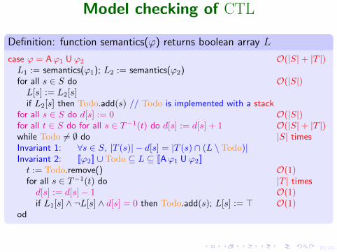
Model checking of CTLDefinition: function semantics(ϕ) returns boolean array L
case ϕ = p ∈ APfor all s ∈ S do L[s] := (p ∈ `(s)) od O(|S|)
case ϕ = ¬ϕ1
L1 := semantics(ϕ1)for all s ∈ S do L[s] := ¬L1[s] od O(|S|)
case ϕ = ϕ1 ∨ ϕ2
L1 := semantics(ϕ1); L2 := semantics(ϕ2)for all s ∈ S do L[s] := L1[s] ∨ L2[s] od O(|S|)
case ϕ = EXϕ1
L1 := semantics(ϕ1)for all s ∈ S do L[s] := ⊥ od O(|S|)for all t ∈ S do if L1[t] then for all s ∈ T−1(t) do L[s] := > O(|S|+ |T |)
case ϕ = AXϕ1
L1 := semantics(ϕ1)for all s ∈ S do L[s] := > od O(|S|)for all t ∈ S do if ¬L1[t] then for all s ∈ T−1(t) do L[s] := ⊥ O(|S|+ |T |)

81/131
Model checking of CTL
Definition: function semantics(ϕ) returns boolean array L
case ϕ = Eϕ1 U ϕ2 O(|S|+ |T |)L1 := semantics(ϕ1); L2 := semantics(ϕ2)for all s ∈ S do O(|S|)L[s] := L2[s]if L2[s] then Todo.add(s) // Todo is implemented with a stack
while Todo 6= ∅ do |S| timesInvariant 1: [[ϕ2]] ∪ Todo ⊆ L ⊆ [[Eϕ1 U ϕ2]]t := Todo.remove() O(1)for all s ∈ T−1(t) do |T | times
if L1[s] ∧ ¬L[s] then Todo.add(s); L[s] := > O(1)od
83/131
Model checking of CTL
Definition: function semantics(ϕ) returns boolean array L
case ϕ = Aϕ1 U ϕ2 O(|S|+ |T |)L1 := semantics(ϕ1); L2 := semantics(ϕ2)for all s ∈ S do O(|S|)L[s] := L2[s]if L2[s] then Todo.add(s) // Todo is implemented with a stack
for all s ∈ S do d[s] := 0 O(|S|)for all t ∈ S do for all s ∈ T−1(t) do d[s] := d[s] + 1 O(|S|+ |T |)while Todo 6= ∅ do |S| timesInvariant 1: ∀s ∈ S, |T (s)| − d[s] = |T (s) ∩ (L \ Todo)|Invariant 2: [[ϕ2]] ∪ Todo ⊆ L ⊆ [[Aϕ1 U ϕ2]]t := Todo.remove() O(1)for all s ∈ T−1(t) do |T | timesd[s] := d[s]− 1 O(1)if L1[s] ∧ ¬L[s] ∧ d[s] = 0 then Todo.add(s); L[s] := > O(1)
od

87/131
Complexity of CTL
Definition: SAT(CTL)
Input: A formula ϕ ∈ CTL
Question: Existence of a model M and a state s such that M, s |= ϕ ?
Theorem: ComplexityI The model checking problem for CTL is PTIME-complete.
I The satisfiability problem for CTL is EXPTIME-complete.

89/131
fairness
Example: Fairness
Only fair runs are of interest
I Each process is enabled infinitely often:∧i
G F runi
I No process stays ultimately in the critical section:∧i
¬F G csi =∧i
G F¬csi
Definition: Fair Kripke structure
M = (S, T, I,AP, `, F1, . . . , Fn) with Fi ⊆ S.
An infinite run σ is fair if it visits infinitely often each Fi

90/131
fair CTL
Definition: Syntax of fair-CTL
ϕ ::= ⊥ | p (p ∈ AP) | ¬ϕ | ϕ ∨ ϕ | Ef Xϕ | Af Xϕ | Ef ϕ U ϕ | Af ϕ U ϕ
Definition: Semantics as a fragment of CTL∗
Let M = (S, T, I,AP, `, F1, . . . , Fn) be a fair Kripke structure.
Let, Ef ϕ = E(FairRun ∧ ϕ) and Af ϕ = A(FairRun→ ϕ)
where FairRun =∧i G FFi
Then, [[ϕ]]f = [[ϕ]]
Lemma: CTLf cannot be expressed in CTL
92/131
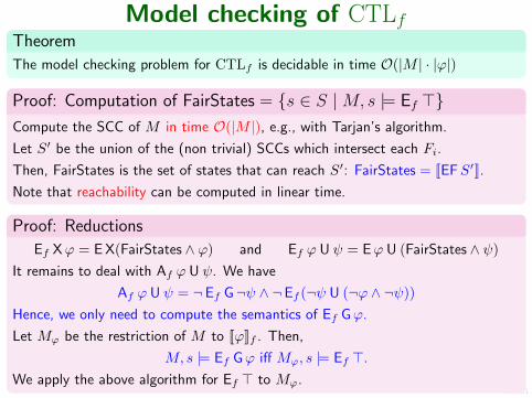
Model checking of CTLfTheorem
The model checking problem for CTLf is decidable in time O(|M | · |ϕ|)
Proof: Computation of FairStates = {s ∈ S |M, s |= Ef >}Compute the SCC of M in time O(|M |), e.g., with Tarjan’s algorithm.
Let S′ be the union of the (non trivial) SCCs which intersect each Fi.
Then, FairStates is the set of states that can reach S′: FairStates = [[EFS′]].
Note that reachability can be computed in linear time.
Proof: Reductions
Ef Xϕ = E X(FairStates ∧ ϕ) and Ef ϕ U ψ = Eϕ U (FairStates ∧ ψ)
It remains to deal with Af ϕ U ψ. We have
Af ϕ U ψ = ¬Ef G¬ψ ∧ ¬Ef (¬ψ U (¬ϕ ∧ ¬ψ))
Hence, we only need to compute the semantics of Ef Gϕ.
Let Mϕ be the restriction of M to [[ϕ]]f . Then,
M, s |= Ef Gϕ iff Mϕ, s |= Ef >.
We apply the above algorithm for Ef > to Mϕ.

94/131
Buchi automataDefinition:
A Buchi automaton (BA) is a tuple A = (Q,Σ, I, T, F ) where
I Q: finite set of states
I Σ: finite set of labels
I I ⊆ Q: set of initial states
I T ⊆ Q× Σ×Q: set of transitions (non-deterministic)
I F ⊆ Q: set of final (repeated) states
Run: ρ = q0, a0, q1, a1, q2, a2, q3, . . . with (qi, ai, qi+1) ∈ T for all i ≥ 0.
ρ is initial if q0 ∈ I.
ρ is final (successful) if qi ∈ F for infinitely many i’s.
ρ is accepting if it is both initial and final.
L(A) = {a0a1a2 · · · ∈ Σω | ∃ ρ = q0, a0, q1, a1, q2, a2, q3, . . . accepting run}
A language L ⊆ Σω is ω-regular if it can be accepted by some Buchi automaton.

96/131
Buchi automata
Properties
Buchi automata are closed under union, intersection, complement.
I Union: trivial
I Intersection: easy (exercise)
I complement: difficult
Let L be the language recognized by the automaton below.
0 1
b
2
b
3
b
· · · n− 2
b
n− 1
b
a a a a
a
Any non deterministic Buchi automaton for Σω \ L has at least 2n states.

97/131
Buchi automataTheorem: BuchiLet L ⊆ Σω be a language. The following are equivalent:
I L is ω-regular
I L is ω-rational, i.e., L is a finite union of languages of the form L1 · Lω2 whereL1, L2 ⊆ Σ+ are rational.
I L is MSO-definable, i.e., there is a sentence ϕ ∈ MSOΣ(<) such thatL = L(ϕ) = {w ∈ Σω | w |= ϕ}.
Exercises:
1. Construct a BA for L(ϕ) where ϕ is the FOΣ(<) sentence
(∀x, (Pa(x)→ ∃y > x, Pa(y)))→ (∀x, (Pb(x)→ ∃y > x, Pc(y)))
2. Given BA for L1 ⊆ Σω and L2 ⊆ Σω, construct BA for
next(L1) = Σ · L1
strict− until(L1, L2) = {uv ∈ Σω | u ∈ Σ+ ∧ v ∈ L2 ∧u′′v ∈ L1 for all u′, u′′ ∈ Σ+ with u = u′u′′}
98/131
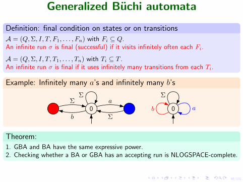
Generalized Buchi automata
Definition: final condition on states or on transitions
A = (Q,Σ, I, T, F1, . . . , Fn) with Fi ⊆ Q.An infinite run σ is final (successful) if it visits infinitely often each Fi.
A = (Q,Σ, I, T, T1, . . . , Tn) with Ti ⊆ T .An infinite run σ is final if it uses infinitely many transitions from each Ti.
Example: Infinitely many a’s and infinitely many b’s
0
Σa
Σb
Σ
0
Σ
ab
Theorem:1. GBA and BA have the same expressive power.2. Checking whether a BA or GBA has an accepting run is NLOGSPACE-complete.

100/131
Unambiguous, Complete, Prophetic (G)BA
Definition: Unambiguous, Complete, Prophetic Buchi automata
A BA or GBA A is unambiguous if every word has at most one accepting run in A.A BA or GBA A is complete if every word has at least one accepting run in A.A BA or GBA A is prophetic if every word has exactly one final run in A.Rem: when I = Q then accepting = final.Hence, when I = Q then prophetic = unambiguous and complete.
Examples: Unambiguous, Complete, PropheticI Finitely many a’s.
I G(a→ F b) with Σ = {a, b, c}.
Proposition:I Prophetic (G)BA are closed under union, intersection, complement.
I A trimmed prophetic (G)BA is co-deterministic and co-complete.
Theorem: Prophetic Buchi automata (Carton-Michel 2003)
Every ω-regular language can be accepted by a prophetic BA.
101/131
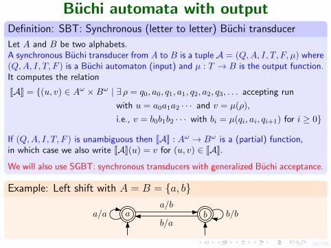
Buchi automata with outputDefinition: SBT: Synchronous (letter to letter) Buchi transducer
Let A and B be two alphabets.A synchronous Buchi transducer from A to B is a tuple A = (Q,A, I, T, F, µ) where(Q,A, I, T, F ) is a Buchi automaton (input) and µ : T → B is the output function.It computes the relation
[[A]] = {(u, v) ∈ Aω ×Bω | ∃ ρ = q0, a0, q1, a1, q2, a2, q3, . . . accepting run
with u = a0a1a2 · · · and v = µ(ρ),
i.e., v = b0b1b2 · · · with bi = µ(qi, ai, qi+1) for i ≥ 0}
If (Q,A, I, T, F ) is unambiguous then [[A]] : Aω → Bω is a (partial) function,in which case we also write [[A]](u) = v for (u, v) ∈ [[A]].
We will also use SGBT: synchronous transducers with generalized Buchi acceptance.
Example: Left shift with A = B = {a, b}
a ba/a b/ba/b
b/a

102/131
Composition of Buchi transducersDefinition: Composition
Let A, B, C be alphabets.Let A = (Q,A, I, T, (Fi)i, µ) be an SGBT from A to B.Let A′ = (Q′, B, I ′, T ′, (F ′j)j , µ
′) be an SGBT from B to C.Then A · A′ = (Q×Q′, A, I × I ′, T ′′, (Fi ×Q′)i, (Q× F ′j)j , µ′′) defined by:
pa/b−−→ q in A and p′
b/c−−→ q′ in A′
(p, p′)a/c−−→ (q, q′) in A · A′
is an SGBT from A to C.When the transducers define functions, we also denote the composition by A′ ◦ A.
Proposition: Composition
1. We have [[A · A′]] = [[A]] · [[A′]].2. If (Q,A, I, T, (Fi)i) and (Q′, B, I ′, T ′, (F ′j)j) are unambiguous (resp.
complete, prophetic) then (Q×Q′, A, I × I ′, T ′′, (Fi ×Q′)i, (Q× F ′j)j) isalso unambiguous (resp. complete, prophetic), and∀u ∈ Aω we have [[A′ ◦ A]](u) = [[A′]]([[A]](u)).

103/131
Product of Buchi transducersDefinition: ProductLet A, B, C be alphabets.Let A = (Q,A, I, T, (Fi)i, µ) be an SGBT from A to B.Let A′ = (Q′, A, I ′, T ′, (F ′j)j , µ
′) be an SGBT from A to C.Then A×A′ = (Q×Q′, A, I × I ′, T ′′, (Fi ×Q′)i, (Q× F ′j)j , µ′′) defined by:
pa/b−−→ q in A and p′
a/c−−→ q′ in A′
(p, p′)a/(b,c)−−−−→ (q, q′) in A · A′
is an SGBT from A to B × C.
Proposition: Product
We identify (B × C)ω with Bω × Cω.
1. We have [[A×A′]] = {(u, v, v′) | (u, v) ∈ [[A]] and (u, v′) ∈ [[A′]]}.2. If (Q,A, I, T, (Fi)i) and (Q′, A, I ′, T ′, (F ′j)j) are unambiguous (resp.
complete, prophetic) then (Q×Q′, A, I × I ′, T ′′, (Fi ×Q′)i, (Q× F ′j)j) isalso unambiguous (resp. complete, prophetic), and∀u ∈ Aω we have [[A×A′]](u) = ([[A]](u), [[A′]](u)).
105/131
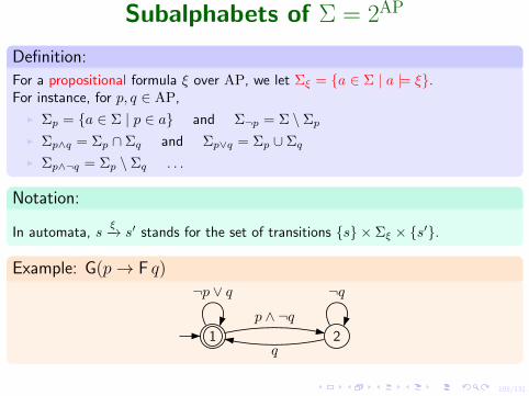
Subalphabets of Σ = 2AP
Definition:
For a propositional formula ξ over AP, we let Σξ = {a ∈ Σ | a |= ξ}.For instance, for p, q ∈ AP,
I Σp = {a ∈ Σ | p ∈ a} and Σ¬p = Σ \ ΣpI Σp∧q = Σp ∩ Σq and Σp∨q = Σp ∪ ΣqI Σp∧¬q = Σp \ Σq . . .
Notation:
In automata, sξ−→ s′ stands for the set of transitions {s} × Σξ × {s′}.
Example: G(p→ F q)
1 2
¬p ∨ q ¬q
p ∧ ¬q
q

106/131
Semantics of LTL with sequential functions
Definition: Semantics of ϕ ∈ LTL(AP, SU, SS)
Let Σ = 2AP and B = {0, 1}.
Define [[ϕ]] : Σω → Bω by [[ϕ]](u) = b0b1b2 · · · with bi =
{1 if u, i |= ϕ
0 otherwise.
Example:
[[p SU q]](∅{q}{p}∅{p}{p}{q}∅{p}{p, q}∅ω) = 1001110110ω
[[X p]](∅{q}{p}∅{p}{p}{q}∅{p}{p, q}∅ω) = 0101100110ω
[[F p]](∅{q}{p}∅{p}{p}{q}∅{p}{p, q}∅ω) = 1111111110ω
The aim is to compute [[ϕ]] with synchronous Buchi transducers (actually, SGBT).
For past formulas, we use deterministic and complete GBA.
For future formulas, we use prophetic GBA.

107/131
Prophetic Buchi automaton for U and SU
Example: A prophetic BA
1 2
3
q p ∧ ¬q
¬q
q
p ∧ ¬q
q¬p ∧ ¬q
¬p ∧ ¬q
Lemma: The BA is prophetic
For all u = a0a1a2 · · · ∈ Σω,there is a unique final run ρ = s0, a0, s1, a1, s2, a2, s3, . . . of A on u.
The run ρ satisfies for all i ≥ 0, si =
1 if u, i |= q
2 if u, i |= ¬q ∧ (p U q)
3 if u, i |= ¬(p U q)

108/131
Synchronous Buchi transducer for U and SUExample:
SBT for [[p U q]]: 1 2
3
q/1 p ∧ ¬q/1
¬q/0
q/1
p ∧ ¬q/1
q/1
¬p ∧ ¬q/0¬p ∧ ¬q/0
SBT for [[p SU q]]: 1 2
3
q/1 p ∧ ¬q/1
¬q/0
q/1
p ∧ ¬q/1
q/0
¬p ∧ ¬q/1¬p ∧ ¬q/1

109/131
Special cases of Until: Future and Next
Example: F q = > U q and X q = ⊥ SU q
1 2
3
q/1 ¬q/1
¬q/0
q/1
¬q/1
q/1
1
3
q/1
¬q/0
q/0¬q/1
Exercise: Give SBT’s for the following formulae:
SF q, SG q, p SR q, p SS q, Y q, G q, p R q, p S q, G(p→ F q).
110/131
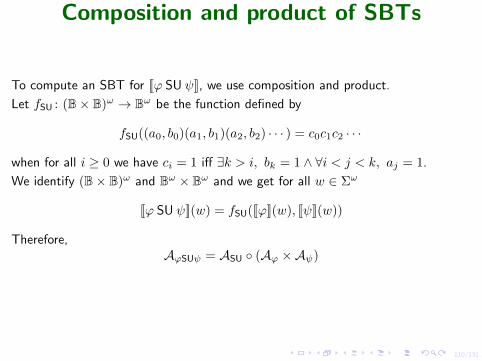
Composition and product of SBTs
To compute an SBT for [[ϕ SU ψ]], we use composition and product.
Let fSU : (B× B)ω → Bω be the function defined by
fSU((a0, b0)(a1, b1)(a2, b2) · · · ) = c0c1c2 · · ·
when for all i ≥ 0 we have ci = 1 iff ∃k > i, bk = 1 ∧ ∀i < j < k, aj = 1.
We identify (B× B)ω and Bω × Bω and we get for all w ∈ Σω
[[ϕ SU ψ]](w) = fSU([[ϕ]](w), [[ψ]](w))
Therefore,AϕSUψ = ASU ◦ (Aϕ ×Aψ)

111/131
From LTL to Buchi automata
Definition: SBT for LTL modalities
I A> from Σ to B = {0, 1}: 0 Σ/1
I Ap from Σ to B = {0, 1}: 0p / 1
¬p / 0
I A¬ from B to B: 00 / 11 / 0
I A∨ from B2 to B: 0
0, 0 / 01, 0 / 10, 1 / 11, 1 / 1
I A∧ from B2 to B: 0
0, 0 / 01, 0 / 00, 1 / 01, 1 / 1

112/131
From LTL to Buchi automata
Definition: SBT for LTL modalities (cont.)
I ASU from B2 to B:Prophetic
1 2
3
0, 1 / 11, 1 / 1
1, 0/1
0, 0 / 01, 0 / 0
0, 1 / 11, 1 / 1
1, 0/1
0, 1 / 01, 1 / 0
0, 0/10, 0/1
I ASS from B2 to B:Deterministic &CompleteNot prophetic
0 10, 0 / 01, 0 / 0
0, 1 / 01, 1 / 0 1, 0 / 1
0, 1 / 11, 1 / 10, 0/1
113/131
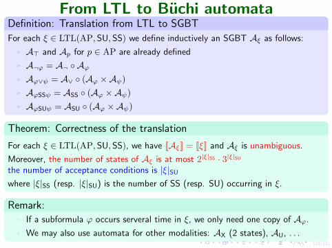
From LTL to Buchi automataDefinition: Translation from LTL to SGBT
For each ξ ∈ LTL(AP,SU,SS) we define inductively an SGBT Aξ as follows:
I A> and Ap for p ∈ AP are already defined
I A¬ϕ = A¬ ◦ AϕI Aϕ∨ψ = A∨ ◦ (Aϕ ×Aψ)
I AϕSSψ = ASS ◦ (Aϕ ×Aψ)
I AϕSUψ = ASU ◦ (Aϕ ×Aψ)
Theorem: Correctness of the translation
For each ξ ∈ LTL(AP,SU,SS), we have [[Aξ]] = [[ξ]] and Aξ is unambiguous.
Moreover, the number of states of Aξ is at most 2|ξ|SS · 3|ξ|SUthe number of acceptance conditions is |ξ|SUwhere |ξ|SS (resp. |ξ|SU) is the number of SS (resp. SU) occurring in ξ.
Remark:I If a subformula ϕ occurs serveral time in ξ, we only need one copy of Aϕ.
I We may also use automata for other modalities: AX (2 states), AU, . . .

114/131
Useful simplifications
Reducing the number of temporal subformulae
(Xϕ) ∧ (Xψ) ≡ X(ϕ ∧ ψ) (Xϕ) SU (Xψ) ≡ X(ϕ SU ψ)
(Gϕ) ∧ (Gψ) ≡ G(ϕ ∧ ψ) G Fϕ ∨ G Fψ ≡ G F(ϕ ∨ ψ)
(ϕ1 SU ψ) ∧ (ϕ2 SU ψ) ≡ (ϕ1 ∧ ϕ2) SU ψ (ϕ SU ψ1) ∨ (ϕ SU ψ2) ≡ ϕ SU (ψ1 ∨ ψ2)
Merging equivalent states
Let A = (Q,Σ, I, T, (Fi)i, µ) be an SGBT and s1, s2 ∈ Q.
We can merge s1 and s2 if they satisfy the same final conditions:
s1 ∈ Fi ⇐⇒ s2 ∈ Fi for all i
and they have the same outgoing transitions: ∀a ∈ Σ, ∀s ∈ Q,
τ1 = (s1, a, s) ∈ T ⇐⇒ τ2 = (s2, a, s) ∈ T and µ(τ1) = µ(τ2)
115/131
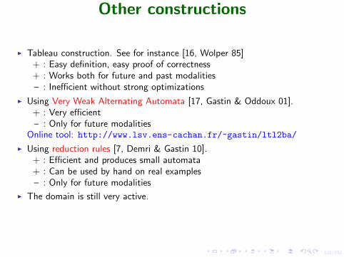
Other constructions
I Tableau construction. See for instance [16, Wolper 85]+ : Easy definition, easy proof of correctness+ : Works both for future and past modalities– : Inefficient without strong optimizations
I Using Very Weak Alternating Automata [17, Gastin & Oddoux 01].+ : Very efficient– : Only for future modalities
Online tool: http://www.lsv.ens-cachan.fr/~gastin/ltl2ba/
I Using reduction rules [7, Demri & Gastin 10].+ : Efficient and produces small automata+ : Can be used by hand on real examples– : Only for future modalities
I The domain is still very active.

116/131
Some References[10] O. Lichtenstein and A. Pnueli.
Checking that finite state concurrent programs satisfy their linear specification.In ACM Symposium PoPL’85, 97–107.
[16] P. Wolper.The tableau method for temporal logic: An overview,Logique et Analyse. 110–111, 119–136, (1985).
[11] A. Sistla and E. Clarke.The complexity of propositional linear temporal logic.Journal of the Association for Computing Machinery. 32 (3), 733–749, (1985).
[17] P. Gastin and D. Oddoux.Fast LTL to Buchi automata translation.In CAV’01, vol. 2102, Lecture Notes in Computer Science, pp. 53–65.Springer, (2001).http://www.lsv.ens-cachan.fr/~gastin/mes-publis.php
[7] S. Demri and P. Gastin.Specification and Verification using Temporal Logics.In Modern applications of automata theory, IISc Research Monographs 2.World Scientific, 2012.http://www.lsv.ens-cachan.fr/~gastin/mes-publis.php
118/131
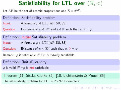
Satisfiability for LTL over (N, <)Let AP be the set of atomic propositions and Σ = 2AP.
Definition: Satisfiability problem
Input: A formula ϕ ∈ LTL(AP,SU,SS)
Question: Existence of w ∈ Σω and i ∈ N such that w, i |= ϕ.
Definition: Initial Satisfiability problem
Input: A formula ϕ ∈ LTL(AP,SU,SS)
Question: Existence of w ∈ Σω such that w, 0 |= ϕ.
Remark: ϕ is satisfiable iff Fϕ is initially satisfiable.
Definition: (Initial) validity
ϕ is valid iff ¬ϕ is not satisfiable.
Theorem [11, Sistla, Clarke 85], [10, Lichtenstein & Pnueli 85]
The satisfiability problem for LTL is PSPACE-complete.

119/131
Model checking for LTL
Definition: Model checking problem
Input: A Kripke structure M = (S, T, I,AP, `)A formula ϕ ∈ LTL(AP,SU,SS)
Question: Does M |= ϕ ?
I Universal MC: M |=∀ ϕ if `(σ), 0 |= ϕ for all initial infinite runs of M .
I Existential MC: M |=∃ ϕ if `(σ), 0 |= ϕ for some initial infinite run of M .
M |=∀ ϕ iff M 6|=∃ ¬ϕ
Theorem [11, Sistla, Clarke 85], [10, Lichtenstein & Pnueli 85]
The Model checking problem for LTL is PSPACE-complete
121/131
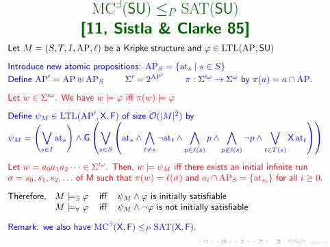
MC∃(SU) ≤P SAT(SU)
[11, Sistla & Clarke 85]Let M = (S, T, I,AP, `) be a Kripke structure and ϕ ∈ LTL(AP,SU)
Introduce new atomic propositions: APS = {ats | s ∈ S}Define AP′ = AP ]APS Σ′ = 2AP′
π : Σ′ω → Σω by π(a) = a ∩AP.
Let w ∈ Σ′ω. We have w |= ϕ iff π(w) |= ϕ
Define ψM ∈ LTL(AP′,X,F) of size O(|M |2) by
ψM =
(∨s∈I
ats
)∧ G
∨s∈S
ats ∧∧t 6=s
¬att ∧∧
p∈`(s)
p ∧∧
p/∈`(s)
¬p ∧∨
t∈T (s)
X att
Let w = a0a1a2 · · · ∈ Σ′ω. Then, w |= ψM iff there exists an initial infinite runσ = s0, s1, s2, . . . of M such that π(w) = `(σ) and ai ∩APS = {atsi} for all i ≥ 0.
Therefore, M |=∃ ϕ iff ψM ∧ ϕ is initially satisfiableM |=∀ ϕ iff ψM ∧ ¬ϕ is not initially satisfiable
Remark: we also have MC∃(X,F) ≤P SAT(X,F).
122/131
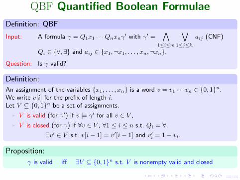
QBF Quantified Boolean Formulae
Definition: QBF
Input: A formula γ = Q1x1 · · ·Qnxnγ′ with γ′ =∧
1≤i≤m
∨1≤j≤ki
aij (CNF)
Qi ∈ {∀,∃} and aij ∈ {x1,¬x1, . . . , xn,¬xn}.
Question: Is γ valid?
Definition:
An assignment of the variables {x1, . . . , xn} is a word v = v1 · · · vn ∈ {0, 1}n.We write v[i] for the prefix of length i.Let V ⊆ {0, 1}n be a set of assignments.
I V is valid (for γ′) if v |= γ′ for all v ∈ V ,
I V is closed (for γ) if ∀v ∈ V , ∀1 ≤ i ≤ n s.t. Qi = ∀,
∃v′ ∈ V s.t. v[i− 1] = v′[i− 1] and v′i = 1− vi.
Proposition:
γ is valid iff ∃V ⊆ {0, 1}n s.t. V is nonempty valid and closed

123/131
QBF ≤P MC∃(U) [11, Sistla & Clarke 85]Let γ = Q1x1 · · ·Qnxn
∧1≤i≤m
∨1≤j≤ki
aij with Qi ∈ {∀,∃} and aij literals.
Consider the KS M :
e0 s1
xt1
xf1
e1 s2
xt2
xf2
e2 · · · sn
xtn
xfn
en
f0
a11
a12...
a1k1
f1
a21
a22...
a2k2
f2 · · · fm−1
am1
am2
...
amkm
fm
Let ψij =
{G(xfk → sk R ¬aij) if aij = xk
G(xtk → sk R ¬aij) if aij = ¬xkand ψ =
∧i,j
ψij .
Let ϕi = G(ei−1 → (¬si−1 U xti) ∧ (¬si−1 U xfi )) and ϕ =∧
i|Qi=∀
ϕi.
Then, γ is valid iff M |=∃ ψ ∧ ϕ.

126/131
Complexity of LTL
Theorem: Complexity of LTL
The following problems are PSPACE-complete:
I SAT(LTL(SU,SS)), MC∀(LTL(SU,SS)), MC∃(LTL(SU,SS))
I SAT(LTL(X,F)), MC∀(LTL(X,F)), MC∃(LTL(X,F))
I SAT(LTL(U)), MC∀(LTL(U)), MC∃(LTL(U))
I The restriction of the above problems to a unique propositional variable
The following problems are NP-complete:
I SAT(LTL(F)), MC∃(LTL(F))

128/131
Complexity of CTL∗
Definition: Syntax of the Computation Tree Logic CTL∗
ϕ ::= ⊥ | p (p ∈ AP) | ¬ϕ | ϕ ∨ ϕ | Xϕ | ϕ U ϕ | Eϕ | Aϕ
Theorem
The model checking problem for CTL∗ is PSPACE-complete
Proof:
PSPACE-hardness: follows from LTL ⊆ CTL∗.
PSPACE-easiness: reduction to LTL-model checking by inductive eliminations ofpath quantifications.

130/131
Satisfiability for CTL∗
Definition: SAT(CTL∗)
Input: A formula ϕ ∈ CTL∗
Question: Existence of a model M and a run σ such that M,σ, 0 |= ϕ ?
Theorem
The satisfiability problem for CTL∗ is 2-EXPTIME-complete

131/131
Outline
Introduction
Models
Temporal Specifications
Satisfiability and Model Checking
5 More on Temporal Specifications