injection moulding simulation -a ﬂnite element · pdf filekeywords: injection molding,...

Department of Construction Sciences

Solid Mechanics

ISRN LUTFD2/TFHF-07/5126-SE(1-81)

INJECTION MOULDING SIMULATION

-A finite element approach to analyse thethermodynamics in an IM tool

Master’s Dissertation by

Rikard Johanssonand

Daniel Konijnendijk

Supervisors

Par Andersson, Tetra Pak Packaging Solutions AB, SwedenEskil Andreasson, Tetra Pak Packaging Solutions AB, Sweden

Anders Harrysson, Div. of Solid Mechanics, Lund University, SwedenUlf Nyman, Div. of Solid Mechanics, Lund University, Sweden

Copyright © 2007 by Div. of Solid Mechanics,Tetra Pak Packaging Solutions AB, Rikard Johansson, Daniel Konijnendijk

Printed by Media-Tryck, Lund University, Lund, SwedenFor information, adress:

Division of Solid Mechanics, Lund University, Box 118, SE-221 00 Lund, SwedenHomepage: http://www.solid.lth.se

Abstract

Injection moulding, IM, is a common manufacturing method and is used to produce awide range of plastic products. Tetra Pak uses this method to create the top part of somepackages. Trying to shorten the research and development stage, Tetra Pak is interestedto investigate the possibility to simulate the manufacturing process of the top part in theFEM software ABAQUS. The FEM approach makes it possible to analyse the thermody-namics within the IM tool and studies could therefore be made to build knowledge of themanufacturing process.

Main objective of this thesis is to create a FE model of the IM tool manufacturing a polymertop, i.e. the top part of the package. Simulated results was evaluated against experimentalvalues measured from an existing IM tool, this to give validity to the FE model. Troughthis work careful studies have been made on how diverse parameters influence the simulatedresults giving a thorough understanding and knowledge of the manufacturing process.

Results from this thesis gave accurate results and an understanding for the thermodynamicin the IM tool, indicating the possibility to simulate the IM process using FEM. Howevera more careful comparison against the existing IM tool is desirable to ensure that the FEmodel’s results have high accuracy. Studies of the simulated results shows that the polymertop can be manufactured within desired cycle time from a thermal perspective. The FEmodel also defined the critical areas in the tool design and improvement proposals wherecreated and evaluated. Results from the improved design give guidelines for future workon the IM tool.

Keywords: Injection Molding, Finite Element Method, Abaqus, Thermal Analysis.

iii

Acknowledgement

This master’s thesis was carried out at Tetra Pak Packaging Solutions AB in Lund incooperation with the Division of Solid Mechanics at Lund University during October 2006to March 2007.

The initiator of this project were MSc Par Andersson, Tetra Pak Packaging Solutions AB,who also worked as supervisor. We would also like to express our deepest gratitude to oursupervisor MSc Eskil Andreasson, Tetra Pak Packaging Solutions AB, for his assistanceand devotion. As supervisors they have provided valuable information, helpful technicalsupport and important feedback. Without these two persons this thesis would have beendifficult to complete.

We would also like to thank our supervisors at the Division of Solid Mechanics, PhDstudent Anders Harrysson and PhD Ulf Nyman for their help with the theory, guidanceand feedback throughout this project.

A great thanks to the Material Analysis Laboratory at Tetra Pak Packaging Solutions ABfor their help with the material properties measurements. Finally we would also like tothank the staff at Tetra Pak in Lund for valuable input and help to the project.

Lund, March 2007

Rikard Johansson Daniel Konijnendijk

v

Nomenclature

A [m2] AreaCp [J/kgK] Specific Heat Capacity at Constant PressureK [J ] Kinematic energyL [m] Lengthm [kg] MassNu Nussels numberPr Prandtls numberQ [J ] Heat input over timeq [W/m2] Heat FluxRe Reynolds numberT [oC] Temperaturet [s] TimeU [J ] Internal energyw [m/s] Flow velocityx, y, z [m] Cartesian Coordinates

Greek Letters

α [W/m2K] Heat transfer coefficient∆ Deltaε Emissivity numberλ [W/mK] Thermal conductivityµ [kg/ms] Dynamic viscosityΦ [W/m2] Emitted heat radiationρ [kg/m3] Densityσ [W/m2K4] Stefan-Boltzmann constantυ [m2/s] Kinematic viscosity

vii

Contents

Abstract iii

Acknowledgement v

Nomenclature vii

1 Introduction 11.1 Problem Formulation . . . . . . . . . . . . . . . . . . . . . . . . . . . . . . 21.2 Objectives . . . . . . . . . . . . . . . . . . . . . . . . . . . . . . . . . . . . 21.3 Limitations and Assumptions . . . . . . . . . . . . . . . . . . . . . . . . . 2

2 Introduction to Injection Moulding 52.1 General Injection Moulding . . . . . . . . . . . . . . . . . . . . . . . . . . 52.2 Injection Compressing Moulding at Tetra Pak . . . . . . . . . . . . . . . . 7

3 Theory 93.1 Introduction to Thermodynamics . . . . . . . . . . . . . . . . . . . . . . . 93.2 Constitutive Material Laws . . . . . . . . . . . . . . . . . . . . . . . . . . 113.3 Constitutive Heat Transfer Laws . . . . . . . . . . . . . . . . . . . . . . . . 123.4 Numeric solution strategy . . . . . . . . . . . . . . . . . . . . . . . . . . . 15

4 Finite Element Modeling 194.1 Geometry . . . . . . . . . . . . . . . . . . . . . . . . . . . . . . . . . . . . 194.2 Thermal Material Properties . . . . . . . . . . . . . . . . . . . . . . . . . . 214.3 Element Mesh . . . . . . . . . . . . . . . . . . . . . . . . . . . . . . . . . . 264.4 Simulation Steps . . . . . . . . . . . . . . . . . . . . . . . . . . . . . . . . 304.5 Surface Interaction and Boundary Conditions . . . . . . . . . . . . . . . . 314.6 Analysis . . . . . . . . . . . . . . . . . . . . . . . . . . . . . . . . . . . . . 34

5 Sensitivity Analysis and Verification of FE Model 355.1 Design of Experiments Analysis . . . . . . . . . . . . . . . . . . . . . . . . 355.2 Experimental tests . . . . . . . . . . . . . . . . . . . . . . . . . . . . . . . 38

ix

6 Results 416.1 FE Simulation of the Injection Moulding Process . . . . . . . . . . . . . . 416.2 FE Simulation Using Steel as Tool Material . . . . . . . . . . . . . . . . . 446.3 Energy Balance . . . . . . . . . . . . . . . . . . . . . . . . . . . . . . . . . 46

7 Improvement Proposals 497.1 Minimization of Heat Input to the Cavity Tool . . . . . . . . . . . . . . . . 497.2 Coolant Temperature . . . . . . . . . . . . . . . . . . . . . . . . . . . . . . 51

8 Discussion 538.1 Conclusion . . . . . . . . . . . . . . . . . . . . . . . . . . . . . . . . . . . . 548.2 Further Work . . . . . . . . . . . . . . . . . . . . . . . . . . . . . . . . . . 55

A ABAQUS/Standard Input File 59

Chapter 1

Introduction

Tetra Pak and their customers, e.g. dairies, focus on the packaging costs. Tetra Paksupplies material and the diaries produce several billions of packages every year, this meansthat reducing milliseconds of the cycle time on every package in production will improveTetra Pak’s position on the market and help both themselves and their customers toincrease profit. Simultaneous, in a world of competitiveness, new and inventive packagedesign to end consumers is important for all actors on the packaging market. This meansthat Tetra Pak has to focus on developing attractive packages to a low competitive cost.

Figure 1.1: 250 ml Tetra Top package with an enlarged top part.

Injection moulding, IM, is a very common manufacturing method and is used to producea wide range of plastic products [1]. Tetra Pak uses this method to create the top part ofsome packages, e.g. Tetra Top, cf. Figure 1.1. By combining a paper-based sleeve witha plastic top, highlighted in Figure 1.1, Tetra Pak has a unique and innovative product,perfectly suited for value-added products [2].

1

CHAPTER 1. INTRODUCTION

1.1 Problem Formulation

Injection moulding tools, the mould where the plastic product is produced, is expensive tomanufacture, i.e. complex geometry create long machining time at a high cost. Changes inIM tool design and IM tool material is common in the research and development phase anda change means that a new IM tool have to be manufactured, which costs both time andmoney. Tetra Pak is therefore interested to investigate the possibility to make accuratecomputer simulations of the plastic top part production process. Changes in IM tool designand IM tool material could then be made before manufacturing the tool and the time toevaluate a new design shortened.

This thesis uses the Finite Element Method, FEM, software ABAQUS v.6.6-1 [3] to sim-ulate the production process of the plastic top. One part of the IM tool, the cavity, ismodelled together with the plastic top and other parts considered needed to make accuratesimulations. The FEM approach also makes it possible to investigate the thermodynamicswithin the cavity tool, i.e. the cavity tool is divided into small elements. Studies couldtherefore be made to find the most critical areas in the cavity tool.

The simulated results in predefined points will be compared with experimental valuesmeasured from an existing IM tool. This will give validity to the FEM model and verify theassumptions made and prove the accuracy of the implemented thermal material parameters.When the IM tool is verified and analysed various proposals will be presented to reducethe time needed to produce one polymer top.

1.2 Objectives

The purpose of this thesis is to create a FE model and simulate the thermodynamics inthe injection moulding process. The thesis will also build knowledge of how a FE model iscreated and propose various strategies to shorten the cooling time in the injection mouldingprocess technique used at Tetra Pak today.

1.3 Limitations and Assumptions

Following limitations and assumptions have been made in this thesis:

� Only one half of the IM tool, the cavity, is modelled.

� No thermal influence on the cavity tool from other parts of the injection mouldingpressing unit.

� The core tool and the coolant are assumed to have a defined constant temperature.

2


� The hot runners are replaced with fixed thermal boundary conditions.

� All heat radiation has been neglected.

� Heat convection from the cavity tool to the surroundings have been neglected.

� No temperature dependent thermal conductivity is used for the plastic top and thecavity tool material.

3


4

Chapter 2

Introduction to Injection Moulding

Injection moulding, IM, is a common manufacturing technique used for plastic products.The manufacturing technique could be used to produce both small as well as large productsin a weight range of 0.000001 kg to 100 kg [1]. The manufacturing process can varydepending on product, this chapter first describes the general IM and then the techniqueused at Tetra Pak.

2.1 General Injection Moulding

An IM machine, also known as press, together with raw plastic material is needed to createa product with the IM technique. The raw material, called resin, is in IM usually shapedas granules. These granules is stored in a feed hopper, a bottom opened bottle which feedsthe press with resin, shown in Figure 2.1. The granules need to be molten to enable aninjection into the tool cavity chamber, i.e. a cavity that reflects the final shape of theplastic product, the IM machine is therefore equipped with a plasticizing unit in orderto melt the resin. Initially in the plasticizing unit a screw, which rotates with help of amotor, melts the granules. Most of the heat is created by friction in the screws rotationbut heating bands are often added to supplement the heat generating. When the granulesare melted the screw inject the polymer into the cavity chamber with an axial movement.

The tool or mould is the term used to describe the production tooling used to produce aplastic product and consists of at least two parts to permit an extraction of the product.The half in contact with the plasticizing unit is named the cavity and the other half isdenoted the core. If the manufactured product have a complex geometry and cannot beformed using only a cavity and a core, moveable sections, named slides, can be used. Aclamping force, i.e. a high pressure, is applied to the two halves to eliminate leakage.The applied pressure is generated from a press, usually with a hydraulic or electric drivingsystem. The press can fasten the tool in either a horizontal or vertical orientation.

5

CHAPTER 2. INTRODUCTION TO INJECTION MOULDING

Figure 2.1: General schematic picture of the IM-process [4].

Hardened steel and aluminium is the most common materials used in tools. Hardenedsteel tools is often more expensive but have a longer lifespan and can therefore produce ahigher number of products before the tool is wear. Aluminium is less expensive and hasthermal material properties that entail a more efficient cooling but the lifespan is shorterwhich results in a lower number of products produced compared to steel. The tool willbe heated when the molten plastic is injected, to transport the energy from the tool andsolidify the plastic the tool usually have drilled cooling channels, often using water ascoolant. Improper cooling can result in burnt products or disordered moulding. In recentyears research for a more efficient cooling system has resulted in more advanced coolingdesign, e.g. milled groove insert [5].

The press, tool, cooling channels, screw, heating bands, feed hopper and resin is all diverseparts of the IM process. The following general steps describe a basic injection cycle:

� The mould is closed shut by a clamping force from the pressing machine.

� A fix volume of molten plastic is injected, with pressure from the screw, into themould chamber.

� The cooling channels in the tool cool and solidify the plastic. The solidification startsat the surface of the plastic and when the center is solidified the product is ready tobe ejected.

� The mould opens and ejector pins placed within the mould assist in the ejection ofthe product.

6


2.2 Injection Compressing Moulding at Tetra Pak

At Tetra Pak, a thin walled polymer top made out of High Density PolyEthylene, HDPE,is produced by using injection compressing moulding.

Tetra Pak uses an IM technique where the polymer is heated in the cavity tool with atype of heating band, called hot runner. To eliminate the solidified plastic between theplasticizing unit and the cavity chamber, i.e. a channel through which the plastic flowstoward the cavity chamber (the sprue), the hot runner is placed in the cavity tool. Ina general IM process this solidified plastic has to be cut or twisted off the manufacturedproduct. By placing the hot runner in the cavity tool, close to the cavity chamber, andregulate the plastic flow with e.g. a gate needle, the plastic between the plasticizing unitand the cavity chamber is eliminated, hence reducing spillage. The warm hot runner placedin the cavity tool with the cold cooling channels creates a conflict between hot and cold.If the cooling channels cool the plastic too efficient in this region the hot runner needs toheat the plastic even more, i.e. more energy is applied to the tool.

Tetra Pak also involves a pressing technique in the IM process. Initially, in the injectionpart of the cycle the cavity volume is larger than in the cooling part, cf. Figure 2.2. Thevolume is regulated by the distance between the cavity tool and the core tool. If thedistance between these tools decreases the cavity volume will also decrease. One of theadvantages of using this pressing method is that there is less distortion in the productwhen finished.

7


a)

b)

c)

d)

Figure 2.2: The four main events in Injection compression moulding. a) An open cavity inthe injection step, b) pressing step, c) cooling step, d) ejection and preparation for a newcycle.

8

Chapter 3

Theory

In this chapter a introduction to thermal theory will be presented. A diverse range ofmaterial is used i.e. polymer, aluminium, steel, air and water. Heat flow, both internaland over surface boundaries depends on diverse natural laws. These laws will be translatedto numerical solvable equations in the following sections. To be able to make a accurateheat transfer analysis three material properties of good quality is needed, density, specificheat and thermal conductivity.

3.1 Introduction to Thermodynamics

Figure 3.1: Arbitrary body.

Study an arbitrary body, cf. Figure 3.1, which is at rest in a cartesian coordinate systemthat follows the center of gravity. The mechanical work input W [J ] is represented by thetraction vector ti on the boundary surface respectively the body force per unit volume bi

acting over the volume on the arbitrary body. The Heat input on the body Q [J ] is definedby r and qn which is heat generated within the body, e.g. inductive heating, respectivelythe heat flow normal to the boundary surface. The arbitrary body can be regarded as aclosed system which the first law of thermal dynamics apply to, i.e.

9

CHAPTER 3. THEORY

∂K + ∂U = Q + W (3.1)

where K denote the kinematic energy [J ] and W is the power input [W ]. Since the bodyis at rest and no forces are interacting with the body, ∂K = 0 and W = 0. U [J ] which isthe internal energy is defined as

∂U =

∫ρudV (3.2)

where u is the internal energy per unit mass. Furthermore, the rate of heat input is definedas

Q =

∫rdV −

∮qndS =

∫rdV −

∮qinidS (3.3)

where r responds to the amount of supplied heat per unit time and volume W/m3. Theheat flux vector is qi [W/m2] and ni is the unit vector normal to the boundary. The firstlaw of thermodynamics (3.1) can now be written as

∫ρudV =

∫rdV −

∮qinidS (3.4)

Note that (3.4) is a global equation. To achieve a local form the Gauss divergence theorem[6] can be used.

∫ (ρu− r +

∂qi

∂xi

)dV = 0 (3.5)

Since the volume V is an arbitrary body, local form of the first law of thermal dynamicsis given by

ρu = r − ∂qi

∂xi

(3.6)

and is commonly known as strong form [7]. Weak form can be achieve by multiplying (3.6)with an arbitrary weight function w and integrate over the body.

∫wρudV =

∫wrdV −

∫w

∂qi

∂xi

dV (3.7)

10

CHAPTER 3. THEORY

∂

∂xi

(wqi) = qi∂w

∂xi

+ w∂qi

∂xi

⇒

⇒ w∂qi

∂xi

=∂

∂xi

(wqi)− qi∂w

∂xi

(3.8)

Now insert (3.8) into (3.7)

∫wρudV =

∫wrdV −

∫∂

∂xi

(wqi)dV +

∫∂w

∂xi

qidV (3.9)

By using Gauss divergence theorem on (3.9) it can be transformed into weak form.[6]

∫wρudV =

∫wrdV −

∮wqinidS +

∫∂w

∂xi

qidV (3.10)

It is noted that no assumption of constitutive nature has been made, i.e. (3.10) holds forany choice of constitutive mode.

3.2 Constitutive Material Laws

To have any practical use of (3.10) constitutive laws needs to be invoked for qi, u andqini = qn. qi is described with Fouriers law [8]

qi = −Kij∂T

∂xj

(3.11)

which explain how the heat flow within a body is transported. The assumed constant Kij

is often known as thermal conductivity λ [W/mK]. It can be seen through the index ofKij that the thermal conductivity within a body is not necessarily isotropic. It is assumedthat the internal energy only depends on temperature

u = u(T ) ⇒ u =∂u

∂T

∂T

∂t(3.12)

and describes how much internal energy u is added due to a change in temperature. ∂u/∂Tis known as specific heat CP (T ) [J/kgK] for thermal calculations of solid bodies. The indexp denotes that constant pressure is assumed [6].

11

CHAPTER 3. THEORY

3.3 Constitutive Heat Transfer Laws

The constitutive laws for heat transfer through a surface have three different natures [9]:

1. Conduction, occurs between solid bodies

2. Convection, occurs when fluids or gases are in motion

3. Radiation, occurs between two bodies with different temperatures

Contact conduction is the ability for two surfaces in contact with each other to transferheat. To describe the heat flow conditions on the boundaries of the body Newton convectionlaw is used,

qn = α(T − T∞) (3.13)

The heat flow between two surfaces is described by

qs = αconduction(Twarm − Tcold) (3.14)

where αcondution [W/m2K] is the surface heat transfer coefficient that depends on physicalconditions and material properties for the contact surface, cf. Figure 3.2.

Figure 3.2: Physical condition that effects αconduction.

There are two types of convection , natural and forced. In natural convection the gravityconstitute the driving force for the flow and in forced convection the flow is generatedby a mechanical force, e.g. a pump. When a fluid is flowing in contact with a surface,e.g. a cooling channel, the surface heat flow depends on the same parameters as contactconduction and is calculated using the same equation as before (3.14). The convectionconstant αconvection do depend on other physical conditions, cf. Figure 3.3. To determinethe convection constant at turbulent pipe flow, both analytical and experimental resultsare to consider.

12

CHAPTER 3. THEORY

Figure 3.3: Physical condition that effects αconvection.

To determine the αconvection analytically a number of non unit constants has to be defined.When a fluid flows along a surface a boundary layer will be established. In the boundaryclosest to the wall a laminar layer will exist through which the heat transport will occur byconduction. If the temperature gradient closest to the wall were known the heat transfercould be calculated with fourier’s law (3.11). Combined with (3.14) following expressionfor the heat transfer coefficient, αconvection, is obtained

αconvection = λ| dT/dx |wall

4T(3.15)

where

4T = Twarm − Tcold (3.16)

Due to the introduction of a absolute temperature gradient in (3.15) no negative numberis needed. The temperature gradient is unfortunately often very hard to measure. Experi-mentally (3.15) is seldom of any use. It is still important for the theoretically understandingof the problem. The temperature gradient along the wall depends on material constantsfor the fluid and by the surface geometry. This will quickly become a lot of parameters toconsider. To simplify this problem a number of non-dimension variables has to be defined.To make (3.15) dimensionless it could be written as

αconvection = λ|dT/dx|wall

∆T= λ

1

L

∣∣∣∣d(T/∆T )

d(x/L)

∣∣∣∣wall

⇒

⇒ αconvectionL

λ=

∣∣∣∣d(T/∆T )

d(x/L)

∣∣∣∣wall

(3.17)

13

CHAPTER 3. THEORY

where L represent the characteristic length [m], e.g. the diameter d in a pipe. Thederivative T/∆T is the temperature variable and x/L the coordinate variable, both non-dimension. The right side of (3.17) is thus a representation of the temperature derivativeat the wall in a non-dimension form. The left side of the equation, i.e. αL/λ, is called theNussel number

Nu =αconvectionL

λ(3.18)

Since measuring the temperature derivative at the wall in e.g. a pipe flow is very compli-cated, the value for Nu has to be decided in other ways. By using the uniformity laws Nucan be expressed as a function of different non-dimension units that are easier to calculate.Once (3.18) is defined the heat transfer coefficient αconvection could easily be calculated.

For geometrically uniform systems the basic equation that describes the temperature andvelocity fields at forced flow can express the temperature field, in a non-dimension form,as a function of two quantities. Reynolds number

Re =wL

υ(3.19)

where w denotes the flowing velocity [m/s] and υ the kinematic viscosity [m2/s]. Prandtlsnumber

Pr =µCP

λ(3.20)

where µ denotes the dynamic viscosity [kg/ms]. The relation between dynamic viscosityand kinematic viscosity is written as υ = µ/ρ. The heat transfer coefficient that is associ-ated with a surface can then be described with (3.18), (3.19) and (3.20) as a function offollowing type

Nu = f(Re, Pr) (3.21)

Through work of McAdams among others, the results have been summarized to somesimple relations. One, often called the Dittus - Boelters correlation, is

Nu = 0.023Re0.8Pr0.4 (3.22)

Which is accurate for moderate temperature differences and for flows where Re ≈ 10 000−120 000, i.e. turbulent flow, and fluids where Pr ≈ 0.7 − 120 in channels with the lengthL ≥ 60di, where di = inner diameter. Fluids with moderate viscosity (µ ≤ 2µwater) canusually use equation (3.22) with flows as low as Re ≥ 3000. Material properties is defined

14

CHAPTER 3. THEORY

at the fluids average temperature, i.e. the means of the fluid temperatures over a cross-section.

The length of the pipe has an influence on the Nussel number. If the pipe is long theinfluence is negligible but if it is shorter than L ≤ 60di a correction factor should be used.

Nu = 0.023Re0.8Pr0.4

(1 + (di/L)0.7

1.05

)

︸︷︷︸Correctionfactor

(3.23)

Heat Radiation is something all bodies around us emitters and is commonly known asinfrared radiation. This radiation is caused by electromagnetic forces generated by theelectron in the body.

The heat radiation emitted is strongly dependent on the bodies absolute surface temper-ature and its characteristics, e.g. colour. A black surface is often considered a perfectradiation surface since it emitters most heat radiation of all surfaces. The emitted heat ra-diation, Φs [W/m2], from a black surface with the area, A, is according to Stefan-Boltzmannlaw

Φs = σAT 4 (3.24)

where T is the surface absolute temperature and σ is Stefan-Boltzmann constant [W/m2K4].

For regular surfaces the emitted heat radiation is less than for a so called black surface. Byusing an emissivity number, ε, that states the relation between actual emitted radiationfrom a surface and the radiation from a black surface the heat radiation could be expressedas

Φs = εσAT 4 (3.25)

where ε depends on surface material and temperature [10].

3.4 Numeric solution strategy

Analytical solutions may exist for simple geometries, this is however often not the casein more complex industrial applications. Therefore, in this section the theories for heattransfer problem will be converted from an analytical to a numerical representation. Thisdue to the complexity of differential equations in most heat transfer problems. The FiniteElement Method, FEM, is a common numerical solution model for solving engineering

15

CHAPTER 3. THEORY

mechanical problems. Initial the weak form (3.10) has to be transformed into matrixformat.

∫wρudV =

∫wrdV −

∮wqndS +

∫∇(w)TqdV (3.26)

By assuming a temperature approximation, with help of a shape function N(x), the weakform (3.26) can now be discretized in space. The Galerkin method is used for the selectionof weight function.

T(x, t) = N(x)a(t)

T(x, t) = N(x)a(t)

∇(T) = B(x)a(t)

w = Nc = cTNT

∇(w) = Bc

With the above expressions (3.26) can now be written as

cT

[(∫NTρu

)−

(−

∫NTqndS +

∫NTrdV +

∫BTqdV

)cT

]= 0 (3.27)

since c is arbitrary it follows that

∫NTρu−

∫BTqdV = fext (3.28)

Since (3.28) is discrete in space but not in time, it is known as the ”semi” discrete FE-equation. To make the discretization in time an implicit method is used

u =u(T )t+∆t − u(t)t

∆t(3.29)

Inserting (3.29) into (3.28) and using the constitutive law (3.11) for the heat flux q resultsin

1∆t

∫ (NTρu(T )t+∆t

)dV +

∫ (BTDBat+∆t

)dV = fext + 1

∆t

∫ (NTρu(T )t

)dV ⇒

⇒ 1∆t


)dV +

∫ (BTDBat+∆t

)dV = f ′ext (3.30)

16

CHAPTER 3. THEORY

To solve (3.30) a Newton method is used. For that a residual function needs to be defined.

Ψ =1

∆t


)dV +

∫ (BTDBat+∆t

)dV − f ′ext = 0 (3.31)

A standard Newton iteration procedure gives

Ψi+1 = Ψi +

(∂Ψ

∂a

)i

∆a = 0

∆a =

(∂Ψi

∂ai

)−1

Ψi

ai+1 = ai + ∆a

where i indicates the iteration number. For a one-dimensional problem, the essence ofthe Newton-Raphson strategy is illustrated in Figure 3.4. The problem is to identifythe solution to the nonlinear equation Ψ(a) = 0. A start value ai is guessed, at thecorresponding point Ψi on the curve Ψ(a), the tangent is determined and this tangentis extrapolated to obtain the next estimate ai+1 for the solution. This process is thenrepeated until the error is within the convergence criteria.

y = Ψ(a)

tangent lines ⋅

⋅⋅⋅ ⋅ ∆aai

ψi

ψi+1ai+1

a

Ψ

Figure 3.4: Scheme over the Newton raphson method.

The term ∂Ψ/∂a is known as the Jacobi matrix and is in this case given by

1

∆t

∫NT ∂u

∂T

∂T

∂adV +

∫BTDBdV =

17

CHAPTER 3. THEORY

1

∆t

∫NT ∂u

∂TNdV +

∫BTDBdV =

∂Ψ

∂a(3.32)

The heat transfer problem is now converted into a numerical representation [6][7].

18

Chapter 4

Finite Element Modeling

The FE-simulations will be performed in the FE-software ABAQUS 6.6-1 [3]. ABAQUScontains several interacting softwares. A combined pre and post processor consisting ofABAQUS/CAE, short for Complete ABAQUS Environment, which is a graphical environ-ment where models can be created and results viewed. ABAQUS/CAE is divided into tendifferent modules, e.g. parts, mesh and boundary condition modules, this to facilitate theuse of the pre processor. These diverse modules will be explained more in detail furtheron in this chapter. As an extension to the modelling in order to obtain results a solver hasto be used. An implicit solver is most common for uncoupled thermal problems, thereforeis the implicit solver ABAQUS/Standard used in the FE simulations.

This chapter describes the modelling procedure for the IM tool. The model consists ofseven parts, the core, the cavity, the polymer top and the four polymer volumes betweenthe hot runner and the cavity tool, these parts will be explained thoroughly later on. Thecooling channels, placed in the cavity, is not a actual part but needs to be considered inthe modelling procedure.

4.1 Geometry

The geometry of the polymer top and the cavity tool is imported from the CAD softwarePro/ENGINEER as a *.stp-file in ABAQUS/CAE. Worth mentioning is that a generalapproach with the SI-units system was used trough the thesis, both in length units andin thermal properties. Simplifications of the geometry were made before the polymer topand the cavity tool was imported. Mainly small details such as holes and round off edgeshave been eliminated. This was done in order to enable a good mesh quality, minimize themesh transitions errors and reduce the number of elements.

A boundary condition at the inner surface of the polymer top define the core tool, sincethe thermal process in the core tool is not included in this assignment. Due to the IM

19

CHAPTER 4. FINITE ELEMENT MODELING

cycle design contains several core tools, each core tool will have efficient cooling enough tobe considered to have a constant temperature.

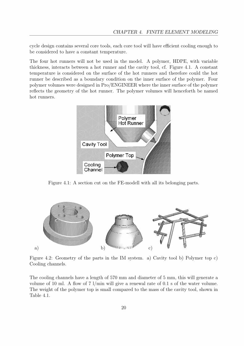
The four hot runners will not be used in the model. A polymer, HDPE, with variablethickness, interacts between a hot runner and the cavity tool, cf. Figure 4.1. A constanttemperature is considered on the surface of the hot runners and therefore could the hotrunner be described as a boundary condition on the inner surface of the polymer. Fourpolymer volumes were designed in Pro/ENGINEER where the inner surface of the polymerreflects the geometry of the hot runner. The polymer volumes will henceforth be namedhot runners.

Figure 4.1: A section cut on the FE-modell with all its belonging parts.

a) b) c)

Figure 4.2: Geometry of the parts in the IM system. a) Cavity tool b) Polymer top c)Cooling channels.

The cooling channels have a length of 570 mm and diameter of 5 mm, this will generate avolume of 10 ml. A flow of 7 l/min will give a renewal rate of 0.1 s of the water volume.The weight of the polymer top is small compared to the mass of the cavity tool, shown inTable 4.1.

20


Table 4.1: Mass and largest diameter of the cavity tool and the polymer top. Volume andlargest diameter of the cooling channels

Cavity tool Polymer top Cooling channelsMass / Volume ∼2.5 kg ∼10 g ∼10 ml

Largest diameter 170 mm ∼80 mm 5 mm (total length 570 mm)

4.2 Thermal Material Properties

Aluminum is the material used in the IM prototype tool and the polymer top part is madefrom High Density PolyEthylene, HDPE. Discussions about using steel as tool materialhave been conducted at Tetra Pak and this section will therefore include steel as an option.

The thermal conductivity, λ [J/mK], is the only material property to be considered in athermal steady state analysis, i.e. when the system have reached equilibrium. Specific heatand density are properties that controls the time needed to reach a steady state level andis used in transient analysis. To illustrate how diverse material properties, e.g. low andhigh thermal conductivity, affect the thermal behavior an example from the everyday lifewill be used. Consider a pot on a hot stove, the pot is filled with water, cf. Figure 4.3. Forsimplicity heat could only move in one dimension and the pot is in perfect contact withthe burner, i.e. the temperature at the bottom of the pot is the same as the burner.

Figure 4.3: Pot on stove, enlarged cut through the pot interacting with burner and water.

In this example the water is continuously replaced in the pot, representing a flow, thetemperature of the water is therefore remained constant. The heat flux q [W/m2], definedin (3.3), is the amount of heat passing through a surface. In steady state analysis qin equals

21


qout, cf. Figure 4.4.

POT

0 L

qin q

out

Twater

Tburner

α

Figure 4.4: Steady state condition where the locations of TBurner, TPot, TWater, α and L isdefined.

Using Fouries Law (3.11) and (3.14), the same as for convection, the following expressionis obtained

qin = λ∆T

L= λ

TBurner − TPot

L, qout = α(TPot − TWater)

TPot =α L TWater + λTBurner

α L + λ(4.1)

By using (4.1) diverse materials temperature gradient could be compared. Figure 4.5 showsthree diverse pot materials, aluminium, steel and HDPE. Using HDPE as a pot materialmay sound strange but remark that this is only an example. The burner heats the outerbottom surface of the pot to 200 �, TBurner, and on the inner surface 20 � water, TWater,interacts through convection with a heat transfer coefficient, α, of 5000 W/m2K on theinner surface of the pot.

The results from Figure 4.5 shows that there is a difference in temperature at L=10 mmbetween aluminium, λ = 165 W/mK and HDPE, λ = 0.32 W/mK. Which of these threematerials is best to use in an IM tool?

The IM tool contains drilled cooling channels. The water in the cooling channels is exposedto heat through convection, same as in the pot. If the temperature gradient between thecooling channels surfaces in the IM tool and the coolant is large, more heat is transferredfrom the IM tool according to (3.14).

If a point on the IM tool is heated the ideal is that the same amount of heat, i.e. in formof a higher temperature, could be seen at the cooling channels surfaces. If this conclusionis implemented on the results from Figure 4.5 aluminium is most suitable as tool material.This because of the small temperature gradient within the material and thereby generatea large temperature gradient between the cooling channels surfaces in the IM tool and thecoolant.

The reader may ask why aluminium has a larger thermal conductivity than HDPE. Thethermal conductivity depends on several physical characteristics. Metallic bonds, like in

22


0 2 4 6 8 100

50

100

150

200

Distance over Pot [mm]

Tem

per

atu

re[d

eg.

Cel

sius]

Aluminium, thermal conductivty 165 W/mK

Steel, thermal conductivity 40 W/mK

HDPE, thermal conductivity 0.5 W/mK

PotBurner Water

Figure 4.5: Temperature gradient over the pot for three different materials, aluminium,steel and HDPE.

aluminium, enhance the thermal conductivity. A high crystalline atomic structure alsoincrease the thermal conductivity [11]. Aluminium has a crystalline atomic structure, i.e.long-range order of atoms. HDPE is mostly crystalline but the structure also involves anamorphous structure, i.e. no long-range order of atoms, especially at higher temperatures.

The thermal conductivity depends on the temperature and the actual phase, i.e. gas,liquid or solid. A solid phase often implies a higher conductivity than a liquid phase [11].As a standard in thermal analysis the thermal conductivity are considered as a constant.In Figure 4.6, it is seen that the change in thermal conductivity is relatively small above400 K, 127 �. In the analysis the polymer will be cooled down below this temperaturebut the error using a constant thermal conductivity is considered small. Observe thatFigure 4.6 represents a general HDPE. In the analysis the thermal conductivity for HDPEis set to 0.32 W/mK according to measurements at Tetra Pak Packaging Solutions ABlaboratory [13]. The temperature level and temperature change in aluminium is consideredlow compared to the melting point for aluminium hence a constant thermal conductivityis used, i.e. 165 W/mK [14].

The IM process contains changes both in boundary conditions and surface interactions.Therefore is a steady state analysis not possible. In a transient analysis two additionalthermal material properties needs to be introduced, density and specific heat.

23


Figure 4.6: Thermal conductivity as a function of temperature for a general HDPE [12].

By multiplying the density, ρ, with the specific heat, Cp, the amount heat Q [J ] neededto heat one cubic meter one Kelvin is obtained. Table 4.2 shows a comparison betweenaluminum, steel and HDPE. Steel needs twice as much energy than aluminium to be heatedone degree, if the volume is constant.

Table 4.2: Thermal conductivity, density, specific heat and density combined with specificheat for Aluminium, Steel and HDPE in room temperature.

λ ρ Cp ρCp[W/mK] [kg/m3] [J/kgK] [J/m3K]

Aluminium 165 2830 890∗ 2.5 · 106

Steel 15− 50 7800− 7900 500− 630 4− 5 · 106

HDPE 0.32 1050 2090∗ 2 · 106

*temperature dependent data used.

It is complicated to make an analytical calculation of the thermal affect from the densityand the specific heat. Using the example with the pot and the FE solver ABAQUS acomparison could be made between aluminium, steel and HDPE. Having a pot with athickness of 10 mm the temperature of a node, i.e. a point on the pot surface interactingwith water, as a function of time, is shown in Figure 4.7. The initial temperature of thepot have been chosen to 50 �. Starting from t = 0 seconds the pot is in perfect contactwith the stoves burner and interacting with water, as earlier.

24


0 1 2 3 4 5 6 7 8 9 100

20

40

60

80

100

120

140

160

180

Time [s]

Tem

per

atu

re[d

eg.

Cel

sius]

Aluminium

Steel

HDPE

WaterBurner Pot

Mesh: 8-node linearheat transfer brick

Figure 4.7: FE simulation of a small piece of the pot.

Aluminium and HDPE reaches a steady state level after 3-5 seconds. Steel have howevera positive derivative after 10 seconds and therefore not reached a steady state level. Aconclusion could therefore be made that a higher specific heat times density increases thetime to reach a steady state level. An analogy could be made with a bath sponge placedunder a jet of water, with water representing heat. If the bath sponge initially is dry theamount water that flow in to the sponge is not the same as the amount of water leaving thesponge. After some time has passed the water flow into the sponge is the same as the waterflow leaving the sponge, i.e. steady state. A high specific heat times density represent asponge with a large volume and vice versa. A sponge with a large volume needs more timeto reach steady state and this is the case for a material with a high density times specificheat.

The thermal conductivity, specific heat and density are all temperature dependent prop-erties. The change in density for the FE simulations temperature interval is considerednegligible. Using temperature dependent data of the HDPE density would in this case alsoresult in an error. The geometry used for the HDPE top is calculated for the top’s finalshape, i.e. at relative low temperature. If a temperature dependent density would havebeen used with a fixed volume on the polymer top, the mass and therefore also the internalenergy, would not be constant during the simulation. Since the density for HDPE increases

25


with increased temperature the internal energy in the polymer top will be reduced usingtemperature dependent density.

Specific heat for a material that changes phase, e.g. from liquid to solid phase, is extremelytemperature dependent. In the IM process HDPE cools from liquid to solid phase andtherefore is temperature dependent data for specific heat of importance. Together withlaboratory scientists from Tetra Pak Packaging Solutions AB [13] a temperature dependentspecific heat for HDPE was obtained, cf. Figure 4.8.

0 50 100 150 200 2500

5

10

15

20

25 Experimental data for HDPE

Temperature [deg. Celsius]

Spec

ific

Hea

t[k

J/kgK

]

Figure 4.8: Scatter plot of temperature dependent specific heat for HDPE from four sam-ples.

As seen in Figure 4.8, a peak in specific heat occurs at approximately 130 �. This verifiesthe importance of using temperature dependent specific heat for HDPE even though theterm ∂u/∂T , described in (3.12), is included and increases calculation time. 4 samples ofHDPE was measured and the difference in internal energy for a fix mass between 80 � to200 � resulted in a 15 % variation between the 4 samples.

4.3 Element Mesh

A proper element mesh is very important since the quality of the mesh have a great impacton the accuracy of the results in the analysis. In general an increased number of elementsyields a better representation of the geometry and allows for a more enhanced elementshape, i.e. no sharp edges etc. A guideline is that more elements improve the accuracy ofthe results but at the cost of longer calculation time.

The difficulties are to use the most suitable type of elements and finding the point ofintersection between an acceptable number of elements and calculation time. In order tobe able to design the mesh more effectively some partitions has been made on different

26


sections of the parts. If a partition of a part is made it will be separated into two cells.Using this, an area of interest are meshed with smaller elements and vice versa and makesthe node seeding much more easy on the edges of the various parts and thereby allowingmore mesh control. This will also enable results reading at interesting areas of the model.

The element type used to mesh the cavity tool is DC3D8, an 8-node linear heat transferbrick, and DC3D4, a 4-node linear heat transfer tetrahedron [15]. The main problemmeshing the cavity tool was to keep the number of elements within an acceptable level.This is due to that the largest part comprises complicated geometry which needs a refinedmesh size to be described accurately.

Figure 4.9: Mesh of the cavity tool consisting of 226 771 elements.

Mainly free structured tetrahedron elements in different sizes are used in the complicatedareas. On the flange a coarser mesh was used, an assumption was made that this areadoes not have much influence on the thermodynamics in the IM process. Moreover, sincethe flange has an uncomplicated geometry, structured brick elements was chosen to savecalculation time.

Figure 4.10: Meshed hot runner consisting of 5 210 elements.

27


The meshing strategy for the hot runners, i.e. the polymer between the actual hot runnerand the cavity tool, was equal to the strategy in the cavity tool. The element type used tomesh the hot runners is solid tetrahedron and brick elements. As seen in Figure 4.10 theupper cylindrical part is structurally meshed with brick elements and the lower more com-plicated geometry freely meshed with tetrahedron elements. Only one element resolutionin thickness is necessary since the heat flow of the hot runner flows from the hot inside(high temperature from the hot runner) to the colder cavity tool.

Regarding the top a new mesh strategy had to be formed in order to create a good meshquality. Three factors have to be considered:

� Cooling from both sides.

� Thin geometry, 0.7 mm.

� Complex geometry.

Figure 4.11: Section cut of the meshed polymer top consisting of 4 884 elements. The tophave two elements in the thickness direction.

Each of these factors by it self does not cause much problem but in combination they do.Because of a thin and complex geometry the amount of elements needs to be quite highto receive proper quality. The fact that there is cooling from both sides means that thetemperature will not be linear within the thickness and a finer resolution in thickness maybe needed.

A simple analysis was made to illustrate how the number of elements in thickness directionaffects the temperature when cooling from two sides. The heat flow is approximated to beone dimensional due to the fact that the polymer is thin, the thermal conductivity is lowand the cooling homogenous. The simple analysis was made by cutting out a small piece,1x1 mm, of the model in the cavity area and simulate one cycle, cf. Figure 4.12.

Initial, at t = 0 seconds, a 200 � polymer top is placed between the 50 � core and cavity

28


Figure 4.12: Small piece of the polymer top placed between the core and the cavity

tool. During the cycle diverse contact properties is used between the two tools and thepolymer. These properties will be explained more in detail further on in this chapter.Simulations with 1, 2 and 15 elements in thickness direction were made. The temperatureon the polymer in contact with the core tool for the different simulations is shown in Figure4.13.

a)0 0.1 0.260 0.640 1.44

50

100

150

200Temperature on polymer in contact with Inner Tool

Time [s]

Tem

per

atu

re[d

eg.

celsiu

s]

1 Element

2 Elements

15 Elements

b)0 0.1 0.2 0.3 0.4 0.5 0.6 0.7

50

51

52

53

54

55

56

57

Length [mm]

Tem

per

atu

re[d

eg.

Cel

sius]

Temperature over the polymer Top at t = 1.44 s

1 Element

2 Element

15 Element

Figure 4.13: Temperature readings a) at contact surface on the polymer. b) through thepolymer thickness at t = 1.44 seconds.

The results shows that the difference between having one or two elements have an impacton the final temperature, at t = 1.44 seconds. However, it also shows that the finaltemperature difference between 2 or 15 elements is small, about 2 %. Initially, the differencebetween 2 and 15 elements is larger than 2 %, but this error is reduced during the cycle.The resolution over the thickness increases with the increased number of elements. Noresolution was obtained using one element but 15 elements resulted in a relative highresolution. Two elements are in this work considered to be accurate enough, this in orderto keep the number of elements to a minimum.

A small approximation of the geometry of the polymer top was done. This by creating

29


a mesh part from the polymer top’s outer surface, which resulted in shell elements. Byextruding these shell elements, in an inward direction, a solid mesh was obtained with ahomogenous thickness of 0.7 mm. The original thickness of the top differs between 0.6 -0.8 mm. With this method a proper quality mesh of the top, with two elements resolutionin thickness, can be created without having to make to big of an approximation.

4.4 Simulation Steps

In an IM process a number of different events will occur. As previously explained thepolymer is injected into the cavity chamber of the tool, which compress the polymer toits final shape. Then the IM tool cools the polymer to such a temperature level that ithas frozen enough to enable a separation from the IM tool. To describe these events inABAQUS a simulation cycle is divided in steps. In this case the cycle consists of four mainsteps, cf. Figure 4.14.

Figure 4.14: Time chart over the steps in a simulation cycle in ABAQUS.

The estimated time period for each step is something that has been decided together withother members of the IM project. Unfortunately boundary conditions and interactionscan not be deactivated in one step and then reactivated again in a later step. Due to thisfact the defined steps cannot be looped, instead a long string of steps has to be createdrepeating the same steps over and over to simulate many cycles after each other, cf. Figure4.15.

30


Figure 4.15: Principal scheme on how the steps are run in ABAQUS.

Following steps explains how one cycle is modelled in ABAQUS:

1. Injection Fix Temp. A very short step with the only purpose to define a homogenoustemperature of 180 � for the polymer. Duration 0.1 ms.

2. Injection represents a real event where the polymer is injected in the moulding cavityfor 99 ms.

3. Substep. A substep is used when a contact pair is removed. This because ABAQUS/Standardstores the corresponding heat fluxes, for every node on the contact surfaces, and au-tomatically ramps these heat fluxes linearly down to zero during the removal step.This ramping down may have the effect of heating up or cooling down the rest of thebody. This problem can be avoided by removing the contact pairs in a very shorttransient step prior to the rest of the analysis, i.e. a sub step. This step can be donein a single increment [16]. Due to these basic conditions the substeps was set to 0.01ms.

4. Pressing represents the event of the two tools, the core and the cavity, pressingtogether after the polymer has been injected. This step has a duration of 160 ms.

5. Substep, same as item 3.

6. Cooling, after the two tool halves are pressed together fully developed cooling existsunder a pressure of approximately 600 bar. This step has a duration of 380 ms.

7. Substep, same as item 3.

8. System preparation represents the cavity tool being removed from the polymer andonly cooling from the core tool exist, under less pressure. This step has a durationof 800 ms.

9. Substep, same as item 3. This is the last step in the simulation cycle. It will seteverything back to zero again, allowing a new cycle to start.

4.5 Surface Interaction and Boundary Conditions

To describe what happens between all the diverse surfaces in the model, boundary con-ditions and interactions has to be defined. In this model there are two different types of

31


interactions. Contact conductance which is defined with a gap conductance and forcedconvection which is defined with a film condition on a surface. These interactions havebeen defined in section 3.3. The core tool and the cooling water in the cavity tool arerepresented with a film condition on the polymers inner surface and the surfaces on thecooling channels in the cavity tool. This means that the core tool and the cooling waterwill be approximated to have a constant temperature, i.e. they can not be heated. This isconsidered to be a small approximation since the extra time between each cycle the samecore tool is used enables an effective cooling. The flow of the cooling water in the coolingchannel is of such proportion that the water will not increase much in temperature. If thewater flow in the cooling channel is set to 7 l/min it will take 0.1 seconds to replace thevolume of water. Convection and heat radiation to the surroundings is in this model notconsidered. A rough estimate shows that there total effect in heat transfer coefficient isas low as 20− 25 W/m2K. Which in contrast to the contact in the cavity and convectionin the cooling channel that are in the area of 2 400 − 30 000 W/m2K have a neglectfulinfluence on the results.

Between two surfaces in contact, e.g. the polymer top and the cavity tool, a contactconduction could be specified. The introduced heat transfer coefficient controls the heatflux passing through the two surfaces, described in (3.14). In contrast with a film condition,contact conduction considers the fact that the bodies will be heated or cooled.

Figure 4.16: Interactions and boundary conditions in FE model.

Initial literature studies and research have set guidelines for the heat transfer coefficients.The ideal would have been to make experiments in a prototype rig to define the valuesfor the heat transfer between the surfaces. But due to the complexity of measuring the

32


Table 4.3: Heat transfer coefficient αconductance [W/m2K] at different steps in cavity.

Cavity tool Core toolStep Top Top

Injection 800 800Pressing 1600 1600Cooling 2400 2400

System Prep. 0 1600

coefficient, and obtain significant results, a decision was made to use published values. Onearticle, from Kamal M.R. et al [17], uses HDPE as mould material. Another article, fromBendada A. [18], shows that the polymers phase change do not affect the heat transfercoefficient as long as the pressure is high in the cavity. These two articles, together withpractical experience at Tetra Pak, work as guidelines for the values of the heat transfercoefficients. During a cycle the conditions will change in the cavity, e.g. pressure andtemperature, this will change the heat transfer coefficient as well, cf. Figure 3.2. To solvethis problem different values for the coefficients will be set for each step in a cycle. Morepressure will induce a higher coefficient and so on.

To decide the heat transfer coefficient for the cooling channels there were more analyticaltheory to lean on, described in section 3.3. Since the ”straight” length of a cooling channelhas a great impact on the turbulence, which affects the heat transfer coefficient, it wasimportant to include this in the calculations. Therefore, the cooling channel is divided insections with different lengths and cross sections, cf. Figure 4.17. For each section of thecooling channel a heat transfer coefficient was calculated, shown in Table 4.4. A decreasein flow velocity generates a heat transfer coefficient decrease.

Figure 4.17: Cooling channel divided in sections, orange color represent low flow sections.

Having the cooling channel divided in sections with different lengths the heat transfer

33


Table 4.4: αconvection[kW/m2K] at different sections in cooling channel.

Section Low Flow 2 3 4 5 6 7 8 9 10 11 12 13 14αV =5 l/min 5 20 29 28 28 29 22 20 19 19 19 19 23 23

αV =7 l/min 5 26 38 37 37 37 28 26 25 25 25 25 30 30

coefficient can be calculated for each section, described in (3.23). The marked ends of eachsection are here called ”low flow” and have an estimated heat transfer coefficient since theflow velocity is unknown.

At the hot runners a boundary condition is set on the inner surface to hold a constanttemperature of 200 �. This condition represents the heat element placed in each hotrunner. Due to energy loss from the hot runner to the cavity the temperature has to beset with a margin over the polymers melting point, ∼130 �. The polymer top is at thebeginning of each cycle given a boundary condition of an initial homogenous temperature,described by item 1 in section ”Step”. All boundary and interactions are shown in theABAQUS input file, cf. Appendix A.

4.6 Analysis

The average simulation time for one IM-cycle of the complete model consisting of 236 865elements with 9 steps is three hours. This when using a total of 4 Central Processing Units,CPU, on a Linux-cluster. One cycle represent 1.44 seconds which means that several cyclesneeds to be simulated until the IM-tool have reached a steady temperature level. To savecalculation time a steady state simulation step is initially used. This symbolizes the startup procedure, i.e. when the tool heats up the polymer in the hot-runner and no polymertops is produced. The steady state step takes less than one hour to simulate.

The use of temperature dependent specific heat increased the simulation time with ap-proximately 200 %. The temperature dependency also made it impossible to use fix timesteps, this resulted in non convergence solutions. Fix time increment is a convenient wayof controlling the simulations and receive results in high frequency at interesting times.The affect that temperature dependent specific heat have on the result is however largerthan not using fix time steps.

34

Chapter 5

Sensitivity Analysis and Verificationof FE Model

When results from the simulations was obtained, questions like ”how the heat transfercoefficient in the injection step affect the temperature of the polymer top?”, ”is this tem-perature plausible?” etc occurred. A Design Of Experiments, DOE, analysis of the cavityand experiments in the prototype rig was therefore performed to evaluate the FE model.

5.1 Design of Experiments Analysis

The only heat transfer coefficient value found in published articles was for the polymerHDPE at fully developed cooling. As previously mentioned the FE model is designed withseveral different simulation steps and diverse magnitudes for the heat transfer coefficientbetween the cavity tool and the polymer top. Numerical values for these different simula-tion steps where set together with Par Andersson, an expert on In-Line Plastic Mouldingat Tetra Pak Packaging Solutions AB.

A DOE was made to evaluate how the values for the heat transfer coefficient in the diversesteps affect the temperature inside and on the polymer top’s susrface. This was made byusing the values from Table 4.3 and set high and low values out of these, shown in Table5.1.

In the injection step a high value of the heat transfer coefficient represent a fully developedcooling with compensation for that only about half of the cavity chamber is in contact withthe polymer (no pressing has occurred). The low value of the heat transfer coefficient inthe injection step is then set so the base line value represent the average of high and low.In the pressing step the high value represent the fact that a fully developed cooling couldbe possible, low is set with the same method as before, i.e. baseline is an average of highand low. The values in the system preparation step are set in the same manner. Observe

35

CHAPTER 5. SENSITIVITY ANALYSIS AND VERIFICATION OF FE MODEL

Table 5.1: Low, baseline and high values for the heat transfer coefficient in the cavity[W/m2K].

Low Baseline HighInjection 400 800 1200Pressing 800 1600 2400Cooling 1200 2400 3600System Preparation 800 1600 2400

that the cavity tool does not interact with the top in this step and values are thereforeonly changed for the core tool. Finally, values for high and low is set in the cooling stepwith the same percentage increase and decrease as previous simulation steps. A 2-level fullfactorial design is now established for the heat transfer coefficients in the cavity.

16 simulations is needed to make a 2-level full factorial design for four diverse controlfactors , i.e. 24 = 16. The statistical program MINITAB [19] was used to make systemizedsimulations. MINITAB helps the user with input to each simulation and also evaluates theresults in a convenient way. The FE model of the simulations is structured as mentionedin the previous chapter. The temperature of the water in the cooling channels is set to 50� and the flow to 7 l/min. Only one cycle was simulated to save simulation time, i.e.total time 1.44 seconds in reality, simulation time is 3 hours. Therefore are the magnitudesof the results not comparable with a continuous IM process, but one cycle is consideredenough to make conclusions of how each part of the cycle, i.e. injection, pressing, coolingand system preparation, affect the final temperature.

Three node temperatures in the injection region of the top was selected as response para-meters, cf. Figure 5.1. One node at the outer surface, one in the center and one at theinner surface facing the core tool.

Figure 5.1: Selected result nodes on the polymer top.

These three temperatures is selected after one cycle is completed, i.e. after 1.44 seconds.Figure 5.2 shows a main effect plot of how a change in heat transfer coefficient affect

36


the final temperature in the diverse nodes. The four different steps is represented with afigure, the temperature for the diverse nodes could be seen on the vertical axis and theheat transfer coefficients from Table 5.1 on the horizontal axis.

800 1600 240050

75

100

125

150Pressing

800 1600 240050

75

100

125

150System Preperation

400 800 120050

75

100

125

150

Tem

per

ature

[deg

.C

elsius]

Injection

1200 2400 360050

75

100

125

150

Heat Transfer Coefficients

Cooling

Outer Node Center Node Inner Node

Figure 5.2: Main effect plot on how the heat transfer coefficient in the cavity affect thepolymer top temperature.

A small gradient means that the heat transfer coefficient have low influence on the tem-perature and vice versa. As seen in Figure 5.2, step injection, the temperature for theouter, center and inner node is almost the same for both a heat transfer coefficient of 400W/m2K and 1200 W/m2K. The same tendency could be seen in the pressing step. Theinjection and the pressing step have therefore a low influence on the final temperature ofthe top. The heat transfer coefficient for the cooling step affect the final temperature themost, i.e. a large gradient. In the system preparation step the node on the inner surfaceis to a larger extent affected by a heat transfer coefficient change than a node on the outersurface. This is a distance effect. The heat transfer coefficient on the outer surface inthe system preparation part is always zero. Since the polymer top have a low thermalconductivity a change in temperature some distance away, e.g. at the inner surface of thepolymer, is of low influence.

Since the values for the heat transfer coefficients in the injection and pressing step havelow influence on the final result these steps are of low importance for the FE model. The

37


certainty of the results also increases due to that the values for the heat transfer coefficientin the injection and pressing step was set with help of experienced persons.

5.2 Experimental tests

Experimental tests were made in the prototype rig to verify the simulation results. Bymeasuring temperatures at different locations on the prototype cavity tool these tempera-tures could be compared to the temperatures at the same location in the simulated IM tool.Due to the complexity of measuring the temperature during a cycle a choice was made tomake the measurements when only the hot runners and the cooling channels where run-ning. This choice eliminates the possibility to verify the heat transfer from the polymertop, but the verification of the heat transfer from the polymer top was made in the designof experiment.

A FLUKE 52 thermometer together with a thermocouple type K was used to measurethe temperature on the cavity tool, cf. Figure 5.3. The test equipment was calibrated at60 � according to EAL publication EA/4-02 [20]. This resulted in an uncertainty of ±0.6� on the results from the test equipment.

Figure 5.3: The thermocouple placed in the cavity.

Temperatures from five different locations on the cavity tool was measured, at one injectionhole, between two injection holes, on the flat lower side of the cavity, on the flange at thecooling inlet and on a the flange at the opposite side of the tool, cf. Figure 5.4.

The current settings from the rig, i.e. hot runner temperature (300 �), cooling flow(5 l/min) and cooling temperature (50 �), was then implemented in the FE model. Bychanging the heat transfer coefficients, between the hot runners/cavity tool and the coolingchannels, with ±20 % a temperature interval was created.

38


Figure 5.4: Schematic picture of the five locations where the temperature was measured.

A 20 % increase of the heat transfer coefficient for the hot runners and a 20 % decrease ofthe heat transfer coefficient for the cooling channels enables a higher energy transportationto the cavity tool and less energy transportation from the cavity tool resulting in a highertemperature. Vice versa, a 20 % decrease of the heat transfer coefficient in the hot runnersand a 20 % increase of the heat transfer coefficient in the cooling channels enables a higherenergy transportation from the cavity tool and less to the cavity tool. These two scenariosare considered a worst/best case. Figure 5.5 shows a scatter plot of the experimentalmeasured locations and the same five locations from the simulated best and worst cases.

Injection Between Injection Flat Side Flange on Cooling Inlet Flange30

35

40

45

50

55

60

65

Measurements Points

Tem

per

atu

re[d

eg.

Cel

sius]

Experiment

Best Case

Worse Case

Figure 5.5: Scatter plot of the experimental and simulated results from the five differentlocations.

The temperatures from the worst case are higher than the best case in all five locations.The difference between worst and best is lower at the flange. This is because of thedistance between the hot runner region, where the increase and decrease of the heat transfercoefficients is made, and the flange. The measured temperatures from the rig are lower than

39


the best case in all measured locations except at the injection location. It is complicated tomeasure an accurate temperature and even though a calibrated equipment was used a lotof other reasons could result in measurement errors. This experiment has given a guidelinethat the results from the simulation are in same level as the prototype rig, although not100 % correct.

40

Chapter 6

Results

Ten injection moulding cycles are simulated to evaluate when the cavity tool and theinjection moulding process reaches a steady temperature level. Steady temperature levelis in this chapter defined by the final temperature after each cycle. The results are thenexplained to give an understanding of the thermodynamics in the IM process. A changein cavity tool material, from aluminium to steel, is made and comparisons of results aredemonstrated. An energy balance is made to analyse how much energy that is applied andremoved from the cavity tool.

6.1 FE Simulation of the Injection Moulding Process

This simulation consist of 10 IM cycles, i.e. the production of 10 polymer tops. Thetotal simulation time for 10 cycles was 30 hours. The coolant temperature is set to 25�, compared to the 50 � used in the experiment, cf. section 5.2. The coolant flow isincreased to 7 l/min, compared to 5 l/min used in the experiment. These settings are morelikely to be used in a continuous IM process. Coolant temperatures under 25 � may causecondensation in the IM process area which is not preferable from an aseptic point of view.

A survey over the temperatures in the system is important for the understanding of thethermodynamics in the IM process. Figure 6.1 shows a section cut of the cavity toolimmediately at the end of the 10th cycle. The highest temperatures in the cavity tool couldbe seen around the injection hole, this area is hence the most critical in the cavity tool.During a cycle the temperature for this area can increase to ∼40 �. As seen in Figure 6.1the temperature varies from 34 � to 26 � , i.e. 1 � to 9 � over the coolant temperature.These results could be compared to the experimental measurements, seen in Figure 5.5,with coolant temperature of 50 � , lower coolant flow (5 l/min instead of 7 l/min) and ahigher hot runner temperature (300 � instead of 200 �). The experimental measurementshows an increased temperature of 11 � to 1 � over the coolant temperature. The

41

CHAPTER 6. RESULTS

temperature on the opposite side of the two cooling channels is low and is therefore ofsmall interest.

NT11

2627282930323334

Figure 6.1: Section cut of the cavity tool in the injection area.

The temperature in the cavity tool is important for the understanding of the thermody-namics, but it is the temperature in and on the top that decides when the polymer topcan be ejected from the cavity tool. Figure 6.2 shows the temperature on the outer surfaceof the polymer top and on the cavity surface of the cavity tool in the injection area, i.e.the warmest zone. The difference between the warmest and coolest zone is ∼2 � on thepolymer top in contact with the cavity tool.

A steady temperature level is reached after only 2 cycles and the top have a final tem-perature of 107 � at the end of a cycle, which could be compared to HDPE’s meltingtemperature of ∼130 �. In Figure 6.3 the 10th and last cycle is enlarged and a centerand inner surface node from the injection area of the polymer top is added to show wherethe final temperature is highest. The center node is placed between the inner and outersurface node, cf. Figure 5.1.

In Figure 6.3, the simulated steps can be interpreted from the different curve derivativeswhich depend on the change of heat transfer coefficient in the cavity chamber during thecycle. An increased heat transfer coefficient increases the temperature derivatives and viceversa. Moreover, a significant reduction of the derivative can be seen in the curvatures whenthe nodes reach temperatures around 135 �, this is because of the peak in the specific heatfor the polymer, i.e. the phase when the polymer is solidified. The highest final temperatureis seen on the outer surface on the polymer, this is because the outer surface is reheatedagain from the center of the polymer top when the cavity tool is removed. A comparisoncan be made with a boiled egg placed in cold water to cool down. The temperature seems

42

CHAPTER 6. RESULTS

1 2 3 4 5 6 7 8 9 100

20

40

60

80

100

120

140

160

180

200

Cycle

Tem

per

atu

re[d

eg.

Cel

sius]

Polymer

Cavity tool

107deg. Celsius

Figure 6.2: Temperature in the injection zone at the polymer top and cavity tool, made ofaluminium, during ten cycles.

Inj. Press. Cooling System Preparation40

60

80

100

120

140

160

180

Time Steps

Tem

per

atu

re[d

eg.

Cel

sius]

Outer surfaceCenterInner surface

Figure 6.3: The temperature for three nodes, outer surface, inner surface and in the centerat the injection zone on the polymer are shown over the last cycle.

cold if a hand is placed around the egg, the heat from the egg is transported to the waterwith relative high heat transfer coefficient. This means that the water cools the surface ofthe egg faster than the egg can transport heat from its hot core to the surface. If the egg

43

CHAPTER 6. RESULTS

is removed from the water to the air, resulting in a lower heat transfer coefficient, the hotcore heats the surface of the egg and it feels hot. The inner surface of the polymer top isalso reheated, although not as much as the outer surface, and the heat transfer coefficient isreduced to 1600 W/m2K. The heat transfer coefficient is the same for the inner and outerpolymer surface in the injection, pressing and cooling step, although the two surfaces showa difference in temperature. This depends on the difference in temperature of the cavitytool and the core tool. While the core tool is assumed to have a constant temperature of25 � the cavity tool is heated.

6.2 FE Simulation Using Steel as Tool Material

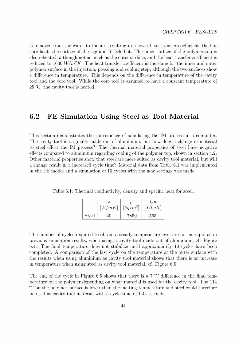
This section demonstrates the convenience of simulating the IM process in a computer.The cavity tool is originally made out of aluminium, but how does a change in materialto steel effect the IM process? The thermal material properties of steel have negativeeffects compared to aluminium regarding cooling of the polymer top, shown in section 4.2.Other material properties show that steel are more suited as cavity tool material, but willa change result in a increased cycle time? Material data from Table 6.1 was implementedin the FE model and a simulation of 10 cycles with the new settings was made.

Table 6.1: Thermal conductivity, density and specific heat for steel.

λ ρ Cp[W/mK] [kg/m3] [J/kgK]

Steel 40 7850 565

The number of cycles required to obtain a steady temperature level are not as rapid as inprevious simulation results, when using a cavity tool made out of aluminium, cf. Figure6.4. The final temperature does not stabilize until approximately 10 cycles have beencompleted. A comparison of the last cycle on the temperature at the outer surface withthe results when using aluminium as cavity tool material shows that there is an increasein temperature when using steel as cavity tool material, cf. Figure 6.5.

The end of the cycle in Figure 6.5 shows that there is a 7 � difference in the final tem-perature on the polymer depending on what material is used for the cavity tool. The 114� on the polymer surface is lower than the melting temperature and steel could thereforebe used as cavity tool material with a cycle time of 1.44 seconds.

44

CHAPTER 6. RESULTS

1 2 3 4 5 6 7 8 9 100

20

40

60

80

100

120

140

160

180

200

Cycles

Tem

per

atu

re[d

eg.

Cel

sius]

Polymer

Cavity tool

114deg. Celsius

Figure 6.4: Temperature in the injection zone at the outer surface of the polymer top andat the cavity surface on the cavity tool during ten cycles, using steel as cavity tool material.

Inj. Press. Cooling System Preparation60

80

100

120

140

160

180

Time [s]

Tem

per

atu

re[d

eg.

Cel

sius]

Steel

Aluminium

delta T = 7deg. Celsius

Figure 6.5: The temperature of the polymer top’s outer surface in the injection zone whenusing either steel or aluminium as cavity tool material.

45

CHAPTER 6. RESULTS

6.3 Energy Balance

If the cavity tool is considered as a closed system an energy balance can be calculated.The hot runners and the polymer top supplies energy to the cavity tool and the coolingchannels transport energy out from the cavity tool. If the system is at steady state thesum of the energy balance equation will be equal to zero at the end of a cycle

QTop + QHot runner −QCooling channel = 0

where QTop denotes the energy from the top, QHot runner the energy from the hot runnersand QCooling channel the energy removed by the cooling channels. Using the simulation withaluminium as cavity tool an energy balance for the last step is calculated. When a contactis specified in ABAQUS, the command HFLA (Heat FLux vector multiplied by the Area)enables the possibility to store the heat transported through the surfaces at every timeincrement. Surfaces with no contact, as the cooling channel’s, could also be pre-selectedwith the command SOH to store the heat transportation. Using this for the hot runners,polymer top and cooling channels an energy balance is obtained, cf. Figure 6.6.

Inj. Press. Cooling System Preparation−1500

−1000

−500

0

500

1000

1500

2000

2500

Time Steps

Hea

t[W

]

Cooling channels

Hot Runners

Polymer Top

Figure 6.6: Power graph for the 10th cycle when using Aluminium as cavity tool material.

A heat rate of approximately 340 W from the hot runners is continuously applied to thecavity tool during the cycle. The polymer top deliverers between 700 to 2000 W and 680to 900 W is removed by the cooling channels. The heat applied from the hot runners andthe heat removed by the cooling channels is almost linear. The heat from the polymertop reflects the steps in the cycle, an increase in heat transfer coefficient increases theheat applied to the tool. Using the graphs in Figure 6.6 and integrating over time, QTop,QHotrunner and QCoolingchannel could be obtained.

46

CHAPTER 6. RESULTS

Table 6.2: Energy balance of the cavity tool.

Energy [J]

QTop 814QHR 482QC.Ch -1133

Total 163

As seen in Table 6.2 the energy balance does not equals zero, this even though a steadytemperature level is reached in the cavity chamber area. The cavity tool weigh 2.5 kg andthe specific heat for Aluminium is 890 J/kgK. Using this, the increased temperature of thecavity tool could be calculated. The results show an average temperature increase of 0.07�.

47

CHAPTER 6. RESULTS

48

Chapter 7

Improvement Proposals

Having seen the results from the original design of the cavity tool improvement proposalswas prepared. A trial to eliminate the negative factors from the original cavity tool design,and thereby receive a lower temperature at the cavity chamber, was made. This will resultin the possibility to cool the polymer top more efficient and enable an earlier ejection fromthe cavity tool, i.e. a reduction of cycle time.

7.1 Minimization of Heat Input to the Cavity Tool

A negative factor is the heat flowing out from the hot runners in to the cavity tool. Thisgives the consequence that more heat has to be generated in the hot runners to keep themelted polymer temperature at an acceptable level, i.e. ∼200 �. As seen in the energybalance the cavity tool is applied with 482 J from the hot runners during a cycle. Theimprovement proposal aims to reduce the heat from the hot runners applied to the cavitytool.

By increasing the diameter of the drilled holes in the cavity tool, for the hot runners,enough space will be created to enable an assembly of a thin walled cylinder with fourflanges, cf. Figure 7.1.

The cylinder is made out of stainless steel, resulting in a high temperature gradient withinthe material because of the low thermal conductivity, shown in section 4.2. The onlycontact between the cylinder and the cavity tool is via the four flanges. Between theflanges air interacts, which have a thermal conductivity of ∼0.025 W/mK. An assumptionis therefore made that no heat is transported through the air. This modification will helpto isolate the upper part of the hot runner.

49

CHAPTER 7. IMPROVEMENT PROPOSALS

Figure 7.1: A section cut of the tool with the isolating (highlighted) cylinder implementedand the thickened polymer at the injection zone.

Table 7.1: Material data for stainless steel.

λ ρ Cp[W/mK] [kg/m3] [J/kgK]

Stainless Steel 14 8000 440

For the lower conical shaped part a small change in dimension on the fixture, the nutthat stabilize the gate needle, will reduce the heat flow. As mentioned earlier in thisreport the polymer is a good isolator. Therefore, by making the layer of melted polymerbetween the hot runner and the cavity chamber slightly thicker, 0.2 mm, a noticeablereduction of the heat flow from the hot runner will hopefully be seen. Simulations with theimprovement proposal is made using the same coolant temperature, coolant flow and hotrunner temperature as previous. Figure 7.2 shows the temperature in the cavity chamberfor the previous and the improved design.

50


a) b)

Figure 7.2: Temperature in the cavity tool made of aluminium using a) original design. b)improved design.

The temperature level is lower for the improved design in the cavity chamber, but thedifference is small. The temperature on the polymer top was compared for the two designsand a negligible change could be seen. However, the heat from the hot runners was reducedwith 50 %, from ∼340 W to ∼170 W but this reduction did not affect the cooling of thepolymer top.

7.2 Coolant Temperature

The improved design resulted in a negligible temperature improvement on the polymertop. However, the energy loss from the hot runners to the tool was reduced with 50 %,this when using a coolant temperature of 25 �. This render the possibility to use a coolantwith a temperature considerably lower than simulated temperatures without any risk toexceed the hot runners maximum power capacity of 1000 W. Unfortunately, if temperaturesunder 25 � is used there is a risk for condensation in the IM surroundings which is notacceptable in an aseptic point of view. If the aseptic subject is solved or disregardedthe improved design enables for a lower coolant temperature which reduces the cycle time.Figure 7.3 shows how the temperature of the cavity and core surface affect the outer surfacetemperature of the polymer top.

A small piece have been cut out from the FE model, same as Figure 4.12 and the diversetemperatures in Figure 7.3 represent the initial cavity tool temperature. A 20 � decreasein temperature of the cavity and core tool reduced the final temperature of the top with11 �. Remark that 10, 20, 30 � is the temperature of the tool, the temperature level forthe coolant has to be lower.

51


0 0.1 0.26 0.64 1.4440

60

80

100

120

140

160

180

Time [s]

Tem

per

atu

re[d

eg.

Cel

sius]

Temperature 10 deg. Celsius



Figure 7.3: The temperature, at the outer surface of a small piece of the polymer top,using different tool temperatures.

52

Chapter 8

Discussion

During the work of creating a FE model a lot of effort was spend on the research of mate-rial data, since this constitute an important part of the modelling. Reliable temperaturedependent data on specific heat for the polymer, HDPE, was of importance because of thediscontinuity around freezing temperature where the specific heat peaks at values signifi-cantly higher than during the rest of the temperatures. Other material data, density andthermal conductivity, in the diverse materials was not significantly temperature dependentand are therefore only as detailed as the time frame of this master thesis allowed. Anassessment made is that good quality data for this work has been gathered and shouldtherefore give an accurate description of the materials behaviour.

There have been some approximations on the geometry for the analysed parts, mainly tofacilitate the work of meshing the parts. The only region where the geometry approximationcan be discussed is on the top. A top is created with a homogenous thickness of 0.7 mmwhich distinguish from the real top that have a various thickness between 0.6-0.8 mm.Because of the low thermal conductivity in the polymer this could have some influence onthe results and should therefore, if possible, be modelled as precise as feasible.

In this model the core tool and the actual hot runners have only been described as con-ditions. These assumptions are made to save calculation time. The actual hot runnersare automatically controlled to supply a constant temperature and the core tool is cooledbetween every IM cycle. This results in a fairly constant thermal state which is describedwith a boundary condition and film condition.

A time chart was created describing all the events occurring during a production cycle.Because of the complexity to model a flow in ABAQUS the FE model includes only onegeometry of the polymer top, this disable the ability to accurately reproduce the eventof the injection and pressing step. Trying to compensate for this flaw values on the heattransfer coefficient was set in order to reduce the heat flow to a more likely level. Astatistical study, DOE, was made where it is presented that the injection and pressing steponly has a modest influence and that it is the cooling and system preparation step that is

53

CHAPTER 8. DISCUSSION

important to reproduce accurately. These results suggest that the approximation done inthe injection and pressing step will not have any severe influence on the results.

Two articles were used to set a value for the heat transfer coefficient in the cooling step. Thefirst article stated a value for the heat transfer coefficient and the second article concludedthat the coefficient is constant during the cooling step. The values for the heat transfercoefficient during the other steps in the cycle were decided together with expertise fromTetra Pak Packaging Solutions AB. Since the influence from the injection and pressing stepis small, shown in the design of experiments, and that it is likely that the value for the heattransfer coefficient in the cooling step is correct, the system preparation step is the onlyuncertain factor. The value on the heat transfer coefficient in the system preparation step,depends on whether the shrinkage of the polymer preserves the contact pressure againstthe core tool or not, when the cavity tool is removed.

One question that was brought up is, if it is necessary to make a simulation of the wholecavity tool and it’s interacting parts. A tremendous advantage will be made in calculationtime if it is possible to focus on only the critical area in this tool and set boundary conditionsthat represent the surroundings from the whole FE model. Successful attempts were madewhere the small model delivered result almost identical to the whole FE model’s results.However, this is for simulation during one cycle only. Trying to simulate a continuousproduction can be difficult since it is hard to predict how the surroundings is affected inthe long term.

8.1 Conclusion

The main objective of this thesis was to investigate if a FE model can be used to simulatethe thermodynamics in an IM process and to obtain knowledge of how constitutive lawsand material data for this application should be defined to receive accurate results. Anexperiment conducted on a test rig was compared with results from the FE simulationmade in ABAQUS. The outcome of this study showed that the thermodynamics withinthe core tool can be simulated delivering results with accuracy of 1-3 �. An extensive partof this report describes in detail which input data is needed and how to perform a thermalanalysis on an arbitrary IM tool, for future projects at Tetra Pak. An extension of thiswork was, for natural reasons, to evaluate the results and highlight the critical areas in thesimulated tool for further development.

The polymer can not be ejected from the cavity tool until a desired temperature is reached.The temperature of the top therefore decides the cooling time needed before ejection.Results from the simulation showed that the injection zones, both on the cavity tool andthe polymer top’s outer surface, reaches highest temperatures and is hence the most criticalarea in the design. The highest final temperature in the polymer top is 107 � when usingaluminium as cavity tool material, this can be compared with∼130 � which is the polymers

54


melting temperature. If a cavity tool made of steel is used an increase of 7 � is received onthe polymer top. From a thermal perspective aluminium is clearly favourable but there areoften mechanical characteristic that forces the use of steel, usually because an aluminiumtool wear to quickly. This possibility, to change tool material, is a demonstration of theadvantages in using FEM instead of having to manufacture the tools which is very costly.A study of the cavity tool made out of aluminium shows that the most critical areas havea temperature of 34 � which is 9 � above the coolants temperature. A constant flow of340 W is flowing from the hot runners into the cavity tool during the cycle which is almost40 % of the total heat input to the cavity tool.

A proposal of a conceivable design was presented where the hot runners was designed witha cylinder, made out of stainless steel, with flanges to create an isolating layer of air. Also,a change in the design of the stabilizing fixture for the gate needle was made. This is madeto enhance the thickness of the isolating polymer in the most critical area of the tool.The outcome of this design showed that the heat loss from the hot runners into the cavitytool was reduced with 50 % and a temperature drop on the cavity tools surface in thecavity chamber with 2 �. These improvements on the cavity tool result in an insignificanttemperature drop on the polymer top.

From these results a conclusion is that the design of the cooling system in the cavity tooltoday is not limiting the cooling time. The area where the highest temperature is presentin the cavity tool is only 10 � above the coolant’s temperature and even if it is designedperfectly the cavity tool can not reach temperatures lower than the coolant temperatureof 25 �. A temperature in the cavity tool of 25 � will only decrease the highest finaltemperature of the top with about 4 �. If the restriction of a minimum temperature of thecoolant, because of condensation, is revoked, this would render the possibility to lower thecoolants temperature, without any risk to exceed the hot runners capacity, and therebyreduce the cooling time. Another problem is the heat in the center (core) of the polymerthickness which is difficult to cool, the center stays isolated by the polymer surface resultingin longer cooling time.

8.2 Further Work

The lowest coolant temperature allowed within the IM process is 25 �. This thesis showsthat the coolant temperature have significant effect on the temperature of the polymertop. It is therefore of further interest and work to enable the possibility to use a coolanttemperature lower than 25 � without effecting the aseptic criteria.

The polymer top have a thermal conductivity of 0.32 W/mK, this relatively low numberprevents a fast heat removal, especially in the center of the polymer top’s thickness. Anincrease of the thermal conductivity would enable a more efficient cooling. The thicknessof the polymer top is also a factor that effect the cooling, a thick top increases the cooling

55


time due too the low thermal conductivity and more mass, i.e. more energy, needs tobe removed. It is therefore of interest to investigate if the thermal conductivity could beincreased, e.g. with a compound, and analyse if a reduction in the thickness of the polymertop could be made.

The heat transfer coefficient in the system preparation step includes an uncertainty. Exper-iments, in whether the shrinkage of the polymer preserves a high contact pressure againstthe core tool, could give more knowledge and input to the FE model.

56

Bibliography

[1] Becker J, Berggren K, Nilsson L-A, Stromvall H-E. Formsprutningsteknik. Stockholm:YFIND; 2000.

[2] Tetra Pak [homepage on the Internet]. Product information Tetra Top [cited 2007 Jan12]. Available from: http://www.tetrapak.com/.

[3] ABAQUS Inc. part of Dassault Systmes Available from: http://www.abaqus.com/.

[4] Georgia Institute of Technology [homepage on the Internet]. [cited 2007 Feb 25] Avail-able from: http://www.me.gatech.edu/jonathan.colton/me4793/injection.pdf

[5] Sun YF, Lee KS, Nee AYC. Design and FEM analysis of the milled groove insertmethod for cooling of plastic injection moulds. Int J Adv Manuf Technol. 2004 May5;24:715-726

[6] Saabye Ottosen N, Petersson H. Introduction to the FINITE ELEMENT METHOD.Prentice Hall Europe; 1992.

[7] Saabye Ottosen N, Ristinmaa M. The Mechanics of Constitutive Modelling: Numericaland thermodynamical topics. vol. 2. Lund: Div. of Solid Mechanichs Lund University;1999.

[8] Jean Baptise Fourier. Thorie analytique de la chaleur. [cited 2007 Jan 23]. Availablefrom: http://www.lub.lu.se/.

[9] Smith EH. Mechnical Engineer’s Reference Book. [database on theInternet] 12th ed. Elsevier: Knovel. c2003 [cited 2006 Dec 20].http://www.knovel.com/knovel2/Toc.jsp?BookID=676&VerticalID=0.

[10] Ekroth I, Granryd E. Tillampad Termodynamik [Applied Thermodynamics]. Stock-holm: Royal Institute of Technology; 2005.

[11] Sunden B. Varmeoverforing [Heat Transfer]. Lund: Studentlitteratur; 2006.

[12] Alberto Naranjo C, Maria del Pilar Noriega E, Juan Diego Sierra M, Juan RodrigoSanz Injection Molding Processing Data. Munich: Carl Hanser Verlag; 2001

57

BIBLIOGRAPHY

[13] Tetra Pak Packaging Solutions AB. Material Data from the department of PM -Material Analysis. Johan Persson. Lab Scientist: 2007 Jan 11.

[14] Uddeholm [homepage on the Internet]. Thermal conductivity and density forALUMEC [cited 2007 Feb 07]. Available from: http://www.uddeholm.se/.

[15] ABAQUS Theory Manual. v6.5. USA: ABAQUS; 2004.

[16] ABAQUS Analysis User’s Manual. v6.5-1. Section 21.2.4

[17] Kamal MR, Mutel AT, Salloum G, Garcia-Rjon A. Heat Transfer Measurement at theMold Surface During Injection Molding of Thermoplastic Melts. McGill University andNational Research Council Canada. Antec 91:483-486

[18] Bendada A, Derdouri A, Lamontagne M, Simard Y. Analysis of thermal contact re-sistance between polymer and mold in injection molding. National Research CouncilCanada. Applied Thermal Engineering 24 (2004):2029-2040

[19] Minitab release 14 for Windows [homepage on the Internet]. [cited 2007 Feb12]. Avail-able from: http://www.minitab.com/.

[20] European co-operation for Accreditation [homepage on theInternet]. [cited 2007 Feb25] Available from: http://www.european-accreditation.org/n1/doc/EA-4-02.pdf

58

Appendix A

ABAQUS/Standard Input File

**** FE Simulation of TETRA PAK’s INJECTION COMPRESSING MOULDING**** written by RIKARD JOHANSSON and Daniel Konijnendijk***Heading** Job name: FE_Model Model name: Version_11*Preprint, echo=NO, model=NO, history=NO, contact=NO****--------------------------------------------------*** R E G U L A T E D P A R A M E T E R S**--------------------------------------------------*PARAMETERch_factor = 1**----------------------****** CAVITY *******----------------------injection = 800*ch_factorpressing = 1600*ch_factorcooling = 2400*ch_factorsystem_prep = 1600*ch_factor**---------------------------------****** COOLING CHANNELS ********---------------------------------cool2=25632*ch_factorcool3=37610*ch_factorcool4=36696*ch_factorcool5=36696*ch_factorcool6=37443*ch_factorcool7=28221*ch_factorcool8=26022*ch_factorcool9=25310*ch_factorcool10=25370*ch_factorcool11=25310*ch_factor

59

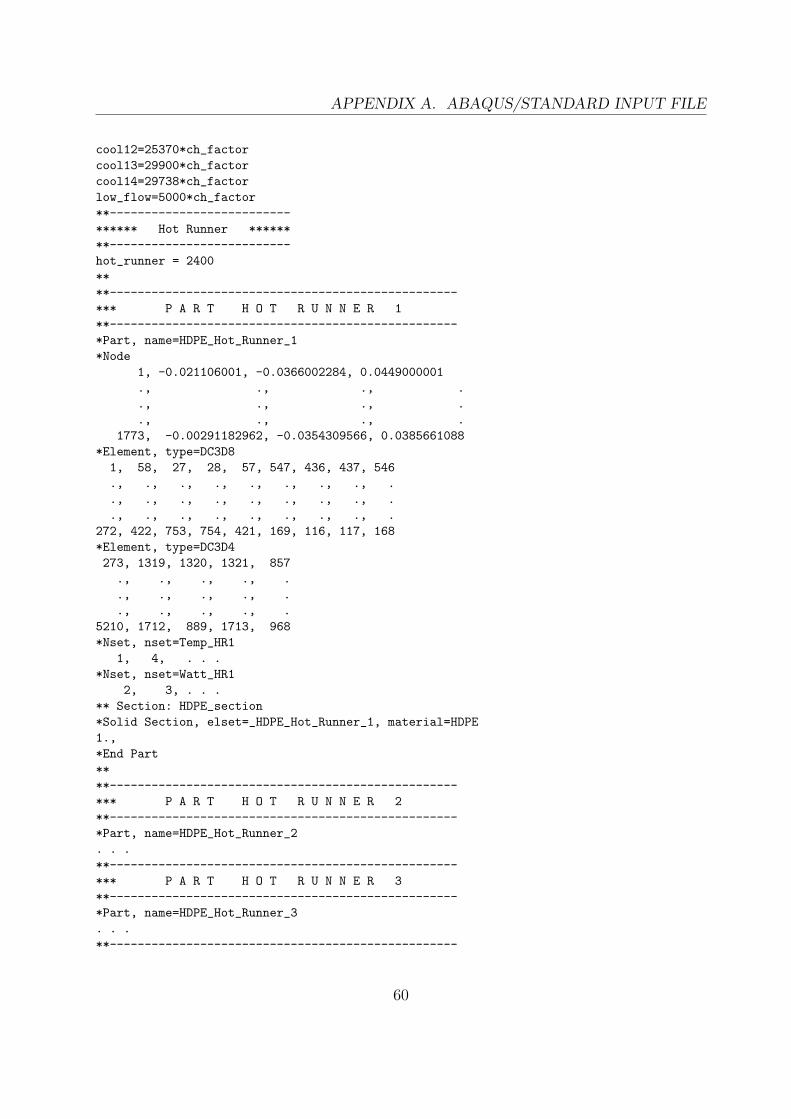
APPENDIX A. ABAQUS/STANDARD INPUT FILE

cool12=25370*ch_factorcool13=29900*ch_factorcool14=29738*ch_factorlow_flow=5000*ch_factor**--------------------------****** Hot Runner ********--------------------------hot_runner = 2400****--------------------------------------------------*** P A R T H O T R U N N E R 1**--------------------------------------------------*Part, name=HDPE_Hot_Runner_1*Node

1, -0.021106001, -0.0366002284, 0.0449000001., ., ., .., ., ., .., ., ., .

1773, -0.00291182962, -0.0354309566, 0.0385661088*Element, type=DC3D8

1, 58, 27, 28, 57, 547, 436, 437, 546., ., ., ., ., ., ., ., .., ., ., ., ., ., ., ., .., ., ., ., ., ., ., ., .

272, 422, 753, 754, 421, 169, 116, 117, 168*Element, type=DC3D4273, 1319, 1320, 1321, 857

., ., ., ., .

., ., ., ., .

., ., ., ., .5210, 1712, 889, 1713, 968*Nset, nset=Temp_HR1

1, 4, . . .*Nset, nset=Watt_HR1

2, 3, . . .** Section: HDPE_section*Solid Section, elset=_HDPE_Hot_Runner_1, material=HDPE1.,*End Part****--------------------------------------------------*** P A R T H O T R U N N E R 2**--------------------------------------------------*Part, name=HDPE_Hot_Runner_2. . .**--------------------------------------------------*** P A R T H O T R U N N E R 3**--------------------------------------------------*Part, name=HDPE_Hot_Runner_3. . .**--------------------------------------------------

60


*** P A R T H O T R U N N E R 4**--------------------------------------------------*Part, name=HDPE_Hot_Runner_4. . .**--------------------------------------------------*** H D P E T O P**--------------------------------------------------*Part, name=HDPE_Top*Node

2535, -0.0207599998, 8.26539601e-11, 0.0492536649., ., ., .., ., ., .., ., ., .

10136, 0.0164417755, 0.0356772803, 0.0132683339*Element, type=DC3D82443, 2535, 2643, 3188, 2562, 5069, 5177, 5722, 5096

., ., ., ., ., ., ., ., .

., ., ., ., ., ., ., ., .

., ., ., ., ., ., ., ., .7326, 7602, 7538, 5705, 5704,10136, 10072, 8239, 8238*Elset, elset=Top_temp, generate2443, 7326, 1

*Elset, elset=Injection, generate2443, 7326, 1

*Surface, type=ELEMENT, name=OffsetElements-Inner_Tool*Surface, type=ELEMENT, name=Cavity_Surface_1...*Surface, type=ELEMENT, name=Cavity_Surface_40** Region: (HDPE_section:Picked)*Elset, elset=_HDPE_Top, internal, generate2443, 7326, 1

** Section: HDPE_section*Solid Section, elset=_HDPE_Top, material=HDPE1.,*End Part****--------------------------------------------------*** C A V I T Y T O O L**--------------------------------------------------*Part, name=cavity_tool*Node

1, 0.0179164279, 0.0624820106, 0.., ., ., .., ., ., .., ., ., .

45831, -0.0103358598,-0.0529843085, 0.00464495085*Element, type=DC3D8

1, 535, 536, 3618, 3610, 3629, 3630, 14106, 14098., ., ., ., ., ., ., ., .

61


., ., ., ., ., ., ., ., .

., ., ., ., ., ., ., ., .2280, 15520, 15536, 15521, 15517, 3612, 3628, 3613, 3609*Element, type=DC3D42281, 15537, 15538, 15539, 15540

., ., ., ., .

., ., ., ., .

., ., ., ., .226771, 39439, 42893, 44189, 45674*Surface, type=ELEMENT, name=Section_2...*Surface, type=ELEMENT, name=Section_14*Surface, type=ELEMENT, name=Section_Low_Flow*Surface, type=ELEMENT, name=H_1...*Surface, type=ELEMENT, name=H_4*Surface, type=ELEMENT, name=Cavity_Tool_Cavity_Surface...*Surface, type=ELEMENT, name=Cavity_Tool_Cavity_Surface_40** Region: (Aluminium_section:Picked)*Elset, elset=cavity_tool, internal, generate

1, 226771, 1** Section: Aluminium_section*Solid Section, elset=cavity_tool, material=Aluminium1.,*End Part****--------------------------------------------------*** A S S E M B L Y**--------------------------------------------------*Assembly, name=Assembly***Instance, name=HDPE_Hot_Runner_1-1, part=HDPE_Hot_Runner_1*End Instance***Instance, name=HDPE_Hot_Runner_2-1, part=HDPE_Hot_Runner_2*End Instance***Instance, name=HDPE_Hot_Runner_3-1, part=HDPE_Hot_Runner_3*End Instance***Instance, name=HDPE_Hot_Runner_4-1, part=HDPE_Hot_Runner_4*End Instance***Instance, name=Cavity_tool-1, part=Cavity_tool

62


*End Instance***Instance, name=HDPE_Top-1, part=HDPE_Top*End Instance***End Assembly****--------------------------------------------------*** M A T E R I A L S**--------------------------------------------------*Material, name=Aluminium*Conductivity165.,*Density2830.,*Specific Heat

840.73, 25.0574840.872, 25.1255841.002, 25.1909

., .

., .

., .946.504, 100.029

*Material, name=HDPE*Conductivity0.32,

*Density1050.,*Specific Heat1801., 50.1800., 51.1818., 52.

., .

., .

., .2287.,200.

****--------------------------------------------------*** I N T E R A C T I O N P R O P E R T I E S**--------------------------------------------------*Surface Interaction, name="Contact Hotrunners"1.,*Gap Conductance<hot_runner>, 0.<hot_runner>, 5.

0.,10.*Surface Interaction, name=Cooling1.,*Gap Conductance<cooling>, 0.<cooling>, 0.005

63


0., 0.01*Surface Interaction, name=Injection1.,*Gap Conductance<injection>, 0.<injection>, 0.005

0., 0.01*Surface Interaction, name=Pressing1.,*Gap Conductance<pressing>, 0.<pressing>, 0.005

0., 0.01*Surface Interaction, name=System_Prep1.,*Gap Conductance0., 0.0., 0.01****--------------------------------------------------*** P R E D E F I N E D F I E L D S**--------------------------------------------------** Name: Initial_Temp Type: Temperature*Initial Conditions, type=TEMPERATURECavity_Tool_and_HR, 50.** Name: Top_temp Type: Temperature*Initial Conditions, type=TEMPERATURETop, 50.****--------------------------------------------------*** I N T E R A C T I O N S**--------------------------------------------------** Interaction: Cavity_Injection*Contact Pair, interaction=InjectionHDPE_Top-1.Cavity_Surface_1, Cavity_tool-1.Cavity_Tool_Cavity_Surface** Interaction: Cavity_Pressing*Contact Pair, interaction=PressingHDPE_Top-1.Cavity_Surface_2, Cavity_tool-1.Cavity_Tool_Cavity_Surface_2** Interaction: Cavity_Cooling*Contact Pair, interaction=CoolingHDPE_Top-1.Cavity_Surface_3, Cavity_tool-1.Cavity_Tool_Cavity_Surface_3** Interaction: Cavity_System_Prep*Contact Pair, interaction=System_PrepHDPE_Top-1.Cavity_Surface_4, Cavity_tool-1.Cavity_Tool_Cavity_Surface_4...** Interaction: Cavity_System_Prep*Contact Pair, interaction=System_PrepHDPE_Top-1.Cavity_Surface_40, Cavity_tool-1.Cavity_Tool_Cavity_Surface_40**

64


** Interaction: H1_HR1*Contact Pair, interaction="Contact Hotrunners", small sliding, type=SURFACE TO SURFACEHDPE_Hot_Runner_1-1.HR_1, Cavity_tool-1.H_1** Interaction: H2_HR2*Contact Pair, interaction="Contact Hotrunners", small sliding, type=SURFACE TO SURFACEHDPE_Hot_Runner_2-1.HR_2, Cavity_tool-1.H_2** Interaction: H3_HR3*Contact Pair, interaction="Contact Hotrunners", small sliding, type=SURFACE TO SURFACEHDPE_Hot_Runner_3-1.HR_3, Cavity_tool-1.H_3** Interaction: H4_HR4*Contact Pair, interaction="Contact Hotrunners", small sliding, type=SURFACE TO SURFACEHDPE_Hot_Runner_4-1.HR_4, Cavity_tool-1.H_4****** ----------------------------------------------------------------**** W A R M U P**** ----------------------------------------------------------------***Step, name="Warm_up", amplitude=RAMP, inc=100000*Heat Transfer, steady state, deltmx=0.0.0001, 1., 1e-07, 1.,**** BOUNDARY CONDITIONS**** Name: Hot_Runner_Temp_1 Type: Temperature*BoundaryHDPE_Hot_Runner_1-1.Temp_HR1, 11, 11, 200.** Name: Hot_Runner_Temp_2 Type: Temperature*BoundaryHDPE_Hot_Runner_2-1.Temp_HR2, 11, 11, 200.** Name: Hot_Runner_Temp_3 Type: Temperature*BoundaryHDPE_Hot_Runner_3-1.Temp_HR3, 11, 11, 200.** Name: Hot_Runner_Temp_4 Type: Temperature*BoundaryHDPE_Hot_Runner_4-1.Temp_HR4, 11, 11, 200.**** INTERACTIONS**** Interaction: Cavity_Injection*Model Change, type=CONTACT PAIR, removeHDPE_Top-1.Cavity_Surface_1, Cavity_tool-1.Cavity_Tool_Cavity_Surface** Interaction: Cavity_Pressing*Model Change, type=CONTACT PAIR, removeHDPE_Top-1.Cavity_Surface_2, Cavity_tool-1.Cavity_Tool_Cavity_Surface_2** Interaction: Cavity_Cooling*Model Change, type=CONTACT PAIR, removeHDPE_Top-1.Cavity_Surface_3, Cavity_tool-1.Cavity_Tool_Cavity_Surface_3** Interaction: Cavity_System_Prep

65


*Model Change, type=CONTACT PAIR, removeHDPE_Top-1.Cavity_Surface_4, Cavity_tool-1.Cavity_Tool_Cavity_Surface_4...** Interaction: Cavity_System_Prep*Model Change, type=CONTACT PAIR, removeHDPE_Top-1.Cavity_Surface_40, Cavity_tool-1.Cavity_Tool_Cavity_Surface_40**** Interaction: Cooling chanel_Low flow*SfilmCavity_tool-1.Low_Flow, F, 25., <low_flow>** Interaction: Cooling chanel_S2*SfilmCavity_tool-1.Section_2, F, 25., <cool2>...** Interaction: Cooling chanel_S14*SfilmCavity_tool-1.Section_14, F, 25., <cool14>****** OUTPUT REQUESTS***Restart, write, frequency=0**** FIELD OUTPUT: F-Output-1***Output, field, frequency=1*Node OutputNT,*Element Output, directions=YESHFL,*Contact OutputHFLA,*Output, history, frequency=0*End Step** ----------------------------------------------------------------**** C Y C L E 1**** ----------------------------------------------------------------****-----------------------------------------------------------------*** STEP: I N J E C T I O N F I X T E M P E R A T U R E**-----------------------------------------------------------------***Step, name=Injection_Fixtemp_1, inc=10000000*Heat Transfer, end=PERIOD, deltmx=5.0.001, 0.001, 1e-07, 0.001,

66


**** BOUNDARY CONDITIONS***BoundaryHDPE_Top, 11, 11, 180.**** INTERACTIONS**** Interaction: Cavity_Injection*Model Change, type=CONTACT PAIR, addHDPE_Top-1.Cavity_Surface_1, Cavity_tool-1.Cavity_Tool_Cavity_Surface** Interaction: HDPE_Cap_Inner_Tool*SfilmHDPE_Top-1.OffsetElements-Inner_Tool, F, 25., <injection>**** OUTPUT REQUESTS***Restart, write, frequency=0*Print, contact=YES**** FIELD OUTPUT: F-Output-1***Output, field, frequency=1*Node OutputNT,*Element Output, directions=YESHFL,*Contact OutputHFLA,*Output, history, frequency=0*End Step****-----------------------------------------------------------------*** STEP: I N J E C T I O N**-----------------------------------------------------------------***Step, name=Injection_1, inc=10000000*Heat Transfer, end=PERIOD, deltmx=5.0.001, 0.099, 9e-07, 0.099,**** BOUNDARY CONDITIONS**** Name: HDPE_Cavity_Injection Type: Temperature*Boundary, op=NEW** Name: Hot_Runner_Temp_1 Type: Temperature*Boundary, op=NEWHDPE_Hot_Runner_1-1.Temp_HR1, 11, 11, 200.** Name: Hot_Runner_Temp_2 Type: Temperature*Boundary, op=NEWHDPE_Hot_Runner_2-1.Temp_HR2, 11, 11, 200.** Name: Hot_Runner_Temp_3 Type: Temperature

67


*Boundary, op=NEWHDPE_Hot_Runner_3-1.Temp_HR3, 11, 11, 200.** Name: Hot_Runner_Temp_4 Type: Temperature*Boundary, op=NEWHDPE_Hot_Runner_4-1.Temp_HR4, 11, 11, 200.**** INTERACTIONS**** Interaction: HDPE_Cap_Inner_Tool*SfilmHDPE_Top-1.OffsetElements-Inner_Tool, F, 25., <injection>***End Step****-----------------------------------------------------------------*** STEP: S U B S T E P**** RAMP OF THE HEAT FLUX ON THE SURFACE**** FOR FURTHER REEDING: SECTION 21.2.4 V.6.5-1**-----------------------------------------------------------------***Step, name=Substep_1*Heat Transfer, end=PERIOD, deltmx=5.1e-05, 1e-05, 1e-10, 1e-05,**** INTERACTIONS**** Interaction: Cavity_Injection*Model Change, type=CONTACT PAIR, removeHDPE_Top-1.Cavity_Surface_1, Cavity_tool-1.Cavity_Tool_Cavity_Surface***End Step****-----------------------------------------------------------------*** STEP: P R E S S I N G**-----------------------------------------------------------------***Step, name=Pressing_1, inc=10000000*Heat Transfer, end=PERIOD, deltmx=5.0.001, 0.16, 1.6e-07, 0.16,**** INTERACTIONS**** Interaction: Cavity_Pressing*Model Change, type=CONTACT PAIR, addHDPE_Top-1.Cavity_Surface_2, Cavity_tool-1.Cavity_Tool_Cavity_Surface_2** Interaction: HDPE_Cap_Inner_Tool*SfilmHDPE_Top-1.OffsetElements-Inner_Tool, F, 25., <pressing>**

68


*End Step****-----------------------------------------------------------------*** STEP: S U B S T E P**-----------------------------------------------------------------***Step, name=Substep_2*Heat Transfer, end=PERIOD, deltmx=5.1e-05, 1e-05, 1e-10, 1e-05,**** Interaction: Cavity_Pressing*Model Change, type=CONTACT PAIR, removeHDPE_Top-1.Cavity_Surface_2, Cavity_tool-1.Cavity_Tool_Cavity_Surface_2***End Step****-----------------------------------------------------------------*** STEP: C O O L I N G**-----------------------------------------------------------------***Step, name=Cooling_1, inc=10000000*Heat Transfer, end=PERIOD, deltmx=5.0.001, 0.38, 3.8e-07, 0.1,**** INTERACTIONS**** Interaction: Cavity_Cooling*Model Change, type=CONTACT PAIR, addHDPE_Top-1.Cavity_Surface_3, Cavity_tool-1.Cavity_Tool_Cavity_Surface_3** Interaction: HDPE_Cap_Inner_Tool*SfilmHDPE_Top-1.OffsetElements-Inner_Tool, F, 25., <cooling>***End Step****-----------------------------------------------------------------*** STEP: S U B S T E P**-----------------------------------------------------------------***Step, name=Substep_3*Heat Transfer, end=PERIOD, deltmx=5.1e-05, 1e-05, 1e-10, 1e-05,**** Interaction: Cavity_Cooling*Model Change, type=CONTACT PAIR, removeHDPE_Top-1.Cavity_Surface_3, Cavity_tool-1.Cavity_Tool_Cavity_Surface_3***End Step****-----------------------------------------------------------------*** STEP: SYSTEM PREPARATION

69


**-----------------------------------------------------------------***Step, name=System_Preparation_1, inc=10000000*Heat Transfer, end=PERIOD, deltmx=5.0.001, 0.8, 8e-07, 0.1,**** INTERACTIONS**** Interaction: Cavity_System_Prep*Model Change, type=CONTACT PAIR, addHDPE_Top-1.Cavity_Surface_4, Cavity_tool-1.Cavity_Tool_Cavity_Surface_4** Interaction: HDPE_Cap_Inner_Tool*SfilmHDPE_Top-1.OffsetElements-Inner_Tool, F, 25., <system_prep>***End Step****-----------------------------------------------------------------*** STEP: S U B S T E P**-----------------------------------------------------------------***Step, name=Substep_4*Heat Transfer, end=PERIOD, deltmx=5.1e-05, 1e-05, 1e-10, 1e-05,**** Interaction: System_Prep*Model Change, type=CONTACT PAIR, removeHDPE_Top-1.Cavity_Surface_4, Cavity_tool-1.Cavity_Tool_Cavity_Surface_4** OUTPUT REQUESTS***Restart, write, frequency=0***End Step**** ----------------------------------------------------------------**** C Y C L E 2**** ----------------------------------------------------------------..........** ----------------------------------------------------------------**

70


** C Y C L E 10**** ----------------------------------------------------------------** ----------------------------------------------------------------**** E N D A N A L Y S**** ----------------------------------------------------------------

71

injection moulding simulation -a ﬂnite element · pdf filekeywords: injection molding,...

Documents