INL/EXT-16-40050

Light Water Reactor Sustainability Program

Probabilistic Fracture Mechanics of Reactor Pressure Vessels with

Populations of Flaws

Benjamin W. Spencer Marie Backman Paul T. Williams

William M. Hoffman Andrea Alfonsi

Terry L. Dickson B. Richard Bass Hilda B. Klasky

September 2016

DOE Office of Nuclear Energy

DISCLAIMER

This information was prepared as an account of work sponsored by an agency of the U.S. Government. Neither the U.S. Government nor any agency thereof, nor any of their employees, makes any warranty, expressed or implied, or assumes any legal liability or responsibility for the accuracy, completeness, or usefulness, of any information, apparatus, product, or process disclosed, or represents that its use would not infringe privately owned rights. References herein to any specific commercial product, process, or service by trade name, trade mark, manufacturer, or otherwise, does not necessarily constitute or imply its endorsement, recommendation, or favoring by the U.S. Government or any agency thereof. The views and opinions of authors expressed herein do not necessarily state or reflect those of the U.S. Government or any agency thereof.

INL/EXT-16-40050

Light Water Reactor Sustainability Program

Probabilistic Fracture Mechanics of Reactor Pressure Vessels with

Populations of Flaws

Benjamin W. Spencer – INL Marie Backman – University of Tennessee

Paul T. Williams – ORNL William M. Hoffman – INL

Andrea Alfonsi – INL Terry L. Dickson – ORNL B. Richard Bass – ORNL Hilda B. Klasky – ORNL

September 2016

Idaho National Laboratory Idaho Falls, Idaho 83415

http://www.inl.gov/lwrs

Prepared for the U.S. Department of Energy Office of Nuclear Energy

Under DOE Idaho Operations Office Contract DE-AC07-05ID14517

ABSTRACT

This report documents recent progress in developing a tool that uses the Grizzly and RAVEN codes to

perform probabilistic fracture mechanics analyses of reactor pressure vessels in light water reactor nuclear

power plants. The Grizzly code is being developed with the goal of creating a general tool that can be

applied to study a variety of degradation mechanisms in nuclear power plant components. Because of the

central role of the reactor pressure vessel (RPV) in a nuclear power plant, particular emphasis is being

placed on developing capabilities to model fracture in embrittled RPVs to aid in the process surrounding

decision making relating to life extension of existing plants.

A typical RPV contains a large population of pre-existing flaws introduced during the manufacturing

process. The use of probabilistic techniques is necessary to assess the likelihood of crack initiation at one

or more of these flaws during a transient event. This report documents development and initial testing

of a capability to perform probabilistic fracture mechanics of large populations of flaws in RPVs using

reduced order models to compute fracture parameters. The work documented here builds on prior efforts

to perform probabilistic analyses of a single flaw with uncertain parameters, as well as earlier work to

develop deterministic capabilities to model the thermo-mechanical response of the RPV under transient

events, and compute fracture mechanics parameters at locations of pre-defined flaws.

The capabilities developed as part of this work provide a foundation for future work, which will

develop a platform that provides the flexibility needed to consider scenarios that cannot be addressed

with the tools used in current practice.

ii

CONTENTS

1 Introduction 1

2 Algorithm Structure 22.1 Overall Structure of Sampling Algorithm . . . . . . . . . . . . . . . . . . . . . . . . . . . 2

2.1.1 FAVOR methodology . . . . . . . . . . . . . . . . . . . . . . . . . . . . . . . . . 2

2.1.2 Grizzly/RAVEN implementation . . . . . . . . . . . . . . . . . . . . . . . . . . . . 3

2.2 Flaw Geometry Sampling . . . . . . . . . . . . . . . . . . . . . . . . . . . . . . . . . . . . 6

2.3 Chemistry Sampling . . . . . . . . . . . . . . . . . . . . . . . . . . . . . . . . . . . . . . 7

2.4 RTNDT Sampling . . . . . . . . . . . . . . . . . . . . . . . . . . . . . . . . . . . . . . . . 8

2.5 Failure Computation . . . . . . . . . . . . . . . . . . . . . . . . . . . . . . . . . . . . . . 9

2.5.1 Surface-breaking Flaw 𝐾𝐼 Calculation . . . . . . . . . . . . . . . . . . . . . . . . . 9

2.5.2 Embedded Flaw 𝐾𝐼 Calculation . . . . . . . . . . . . . . . . . . . . . . . . . . . . 11

3 Benchmarking 133.1 Individual Flaw CPI Calculations . . . . . . . . . . . . . . . . . . . . . . . . . . . . . . . . 13

3.2 Flaw Sampling . . . . . . . . . . . . . . . . . . . . . . . . . . . . . . . . . . . . . . . . . 13

3.3 Overall CPI Calculations . . . . . . . . . . . . . . . . . . . . . . . . . . . . . . . . . . . . 14

4 Summary and Future Development 174.1 Summary of Current Developments . . . . . . . . . . . . . . . . . . . . . . . . . . . . . . 17

4.2 Planned future work . . . . . . . . . . . . . . . . . . . . . . . . . . . . . . . . . . . . . . . 17

4.3 Benefits of this approach . . . . . . . . . . . . . . . . . . . . . . . . . . . . . . . . . . . . 17

5 References 19

iii

FIGURES

1 Flowchart of algorithm used by FAVOR for probabilistic fracture mechanics with a flaw

population . . . . . . . . . . . . . . . . . . . . . . . . . . . . . . . . . . . . . . . . . . . . 4

2 Flowchart of algorithm used by Grizzly/RAVEN for probabilistic fracture mechanics with

a flaw population. Cross-hatched nodes represent capabilities that have not yet been imple-

mented. . . . . . . . . . . . . . . . . . . . . . . . . . . . . . . . . . . . . . . . . . . . . . 5

3 Difference in CPI between FAVOR and Grizzly in a deterministic analysis. . . . . . . . . . . 13

4 Distributions of flaw characteristics in an RPV realization in Grizzly and FAVOR. The total

number of flaws was 19259 in both Grizzly and FAVOR. . . . . . . . . . . . . . . . . . . . 14

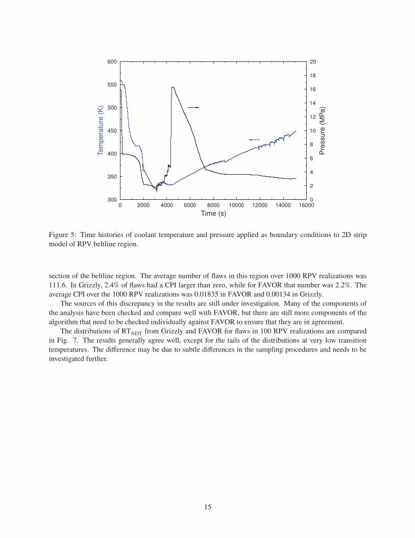
5 Time histories of coolant temperature and pressure applied as boundary conditions to 2D

strip model of RPV beltline region. . . . . . . . . . . . . . . . . . . . . . . . . . . . . . . . 15

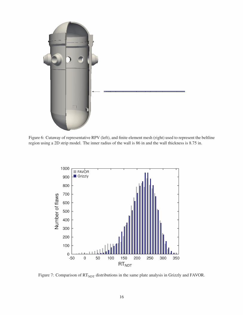
6 Cutaway of representative RPV (left), and finite element mesh (right) used to represent the

beltline region using a 2D strip model. The inner radius of the wall is 86 in and the wall

thickness is 8.75 in. . . . . . . . . . . . . . . . . . . . . . . . . . . . . . . . . . . . . . . . 16

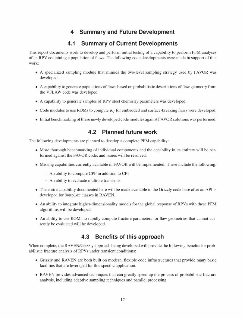
7 Comparison of RTNDT distributions in the same plate analysis in Grizzly and FAVOR. . . . . 16

iv

ACRONYMS

CPI Conditional Probability of Initiation

INL Idaho National Laboratory

LWR Light Water Reactor

LWRS Light Water Reactor Sustainability

ORNL Oak Ridge National Laboratory

PFM Probabilistic Fracture Mechanics

PTS Pressurized Thermal Shock

PWR Pressurized Water Reactor

RISMC Risk-Informed Safety Margin Characterization

ROM Reduced Order Model

RPV Reactor Pressure Vessel

RSM Response Surface Methodology

SIFIC Stress Intensity Factor Influence Coefficient

v

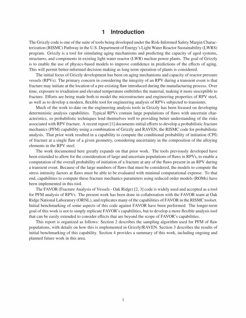
1 Introduction

The Grizzly code is one of the suite of tools being developed under the Risk-Informed Safety Margin Charac-

terization (RISMC) Pathway in the U.S. Department of Energy’s Light Water Reactor Sustainability (LWRS)

program. Grizzly is a tool for simulating aging mechanisms and predicting the capacity of aged systems,

structures, and components in existing light water reactor (LWR) nuclear power plants. The goal of Grizzly

is to enable the use of physics-based models to improve confidence in predictions of the effects of aging.

This will permit better-informed decision making as long term operation of plants is considered.

The initial focus of Grizzly development has been on aging mechanisms and capacity of reactor pressure

vessels (RPVs). The primary concern in considering the integrity of an RPV during a transient event is that

fracture may initiate at the location of a pre-existing flaw introduced during the manufacturing process. Over

time, exposure to irradiation and elevated temperature embrittles the material, making it more susceptible to

fracture. Efforts are being made both to model the microstructure and engineering properties of RPV steel,

as well as to develop a modern, flexible tool for engineering analysis of RPVs subjected to transients.

Much of the work to-date on the engineering analysis tools in Grizzly has been focused on developing

deterministic analysis capabilities. Typical RPVs contain large populations of flaws with uncertain char-

acteristics, so probabilistic techniques lend themselves well to providing better understanding of the risks

associated with RPV fracture. A recent report [1] documents initial efforts to develop a probabilistic fracture

mechanics (PFM) capability using a combination of Grizzly and RAVEN, the RISMC code for probabilistic

analysis. That prior work resulted in a capability to compute the conditional probability of initiation (CPI)

of fracture at a single flaw of a given geometry, considering uncertainty in the composition of the alloying

elements in the RPV steel.

The work documented here greatly expands on that prior work. The tools previously developed have

been extended to allow for the consideration of large and uncertain populations of flaws in RPVs, to enable a

computation of the overall probability of initiation of a fracture at any of the flaws present in an RPV during

a transient event. Because of the large numbers of flaws that must be considered, the models to compute the

stress intensity factors at flaws must be able to be evaluated with minimal computational expense. To that

end, capabilities to compute these fracture mechanics parameters using reduced order models (ROMs) have

been implemented in this tool.

The FAVOR (Fracture Analysis of Vessels - Oak Ridge) [2, 3] code is widely used and accepted as a tool

for PFM analysis of RPVs. The present work has been done in collaboration with the FAVOR team at Oak

Ridge National Laboratory (ORNL), and replicates many of the capabilities of FAVOR in the RISMC toolset.

Initial benchmarking of some aspects of this code against FAVOR have been performed. The longer-term

goal of this work is not to simply replicate FAVOR’s capabilities, but to develop a more flexible analysis tool

that can be easily extended to consider effects that are beyond the scope of FAVOR’s capabilities.

This report is organized as follows: Section 2 describes the sampling algorithm used for PFM of flaw

populations, with details on how this is implemented in Grizzly/RAVEN. Section 3 describes the results of

initial benchmarking of this capability. Section 4 provides a summary of this work, including ongoing and

planned future work in this area.

1

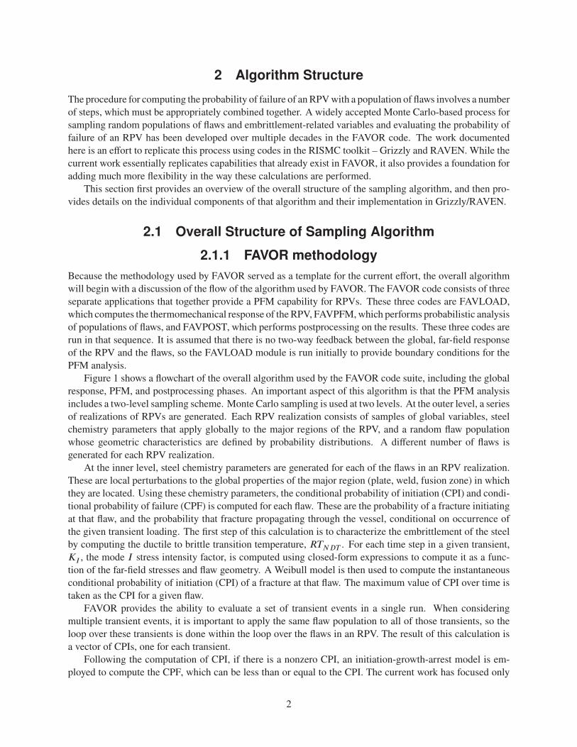
2 Algorithm Structure

The procedure for computing the probability of failure of an RPV with a population of flaws involves a number

of steps, which must be appropriately combined together. A widely accepted Monte Carlo-based process for

sampling random populations of flaws and embrittlement-related variables and evaluating the probability of

failure of an RPV has been developed over multiple decades in the FAVOR code. The work documented

here is an effort to replicate this process using codes in the RISMC toolkit – Grizzly and RAVEN. While the

current work essentially replicates capabilities that already exist in FAVOR, it also provides a foundation for

adding much more flexibility in the way these calculations are performed.

This section first provides an overview of the overall structure of the sampling algorithm, and then pro-

vides details on the individual components of that algorithm and their implementation in Grizzly/RAVEN.

2.1 Overall Structure of Sampling Algorithm

2.1.1 FAVOR methodologyBecause the methodology used by FAVOR served as a template for the current effort, the overall algorithm

will begin with a discussion of the flow of the algorithm used by FAVOR. The FAVOR code consists of three

separate applications that together provide a PFM capability for RPVs. These three codes are FAVLOAD,

which computes the thermomechanical response of the RPV, FAVPFM, which performs probabilistic analysis

of populations of flaws, and FAVPOST, which performs postprocessing on the results. These three codes are

run in that sequence. It is assumed that there is no two-way feedback between the global, far-field response

of the RPV and the flaws, so the FAVLOAD module is run initially to provide boundary conditions for the

PFM analysis.

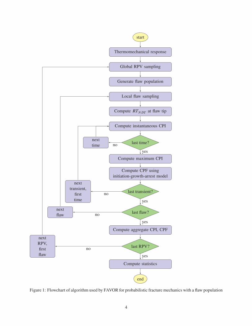
Figure 1 shows a flowchart of the overall algorithm used by the FAVOR code suite, including the global

response, PFM, and postprocessing phases. An important aspect of this algorithm is that the PFM analysis

includes a two-level sampling scheme. Monte Carlo sampling is used at two levels. At the outer level, a series

of realizations of RPVs are generated. Each RPV realization consists of samples of global variables, steel

chemistry parameters that apply globally to the major regions of the RPV, and a random flaw population

whose geometric characteristics are defined by probability distributions. A different number of flaws is

generated for each RPV realization.

At the inner level, steel chemistry parameters are generated for each of the flaws in an RPV realization.

These are local perturbations to the global properties of the major region (plate, weld, fusion zone) in which

they are located. Using these chemistry parameters, the conditional probability of initiation (CPI) and condi-

tional probability of failure (CPF) is computed for each flaw. These are the probability of a fracture initiating

at that flaw, and the probability that fracture propagating through the vessel, conditional on occurrence of

the given transient loading. The first step of this calculation is to characterize the embrittlement of the steel

by computing the ductile to brittle transition temperature, 𝑅𝑇𝑁𝐷𝑇 . For each time step in a given transient,

𝐾𝐼 , the mode 𝐼 stress intensity factor, is computed using closed-form expressions to compute it as a func-

tion of the far-field stresses and flaw geometry. A Weibull model is then used to compute the instantaneous

conditional probability of initiation (CPI) of a fracture at that flaw. The maximum value of CPI over time is

taken as the CPI for a given flaw.

FAVOR provides the ability to evaluate a set of transient events in a single run. When considering

multiple transient events, it is important to apply the same flaw population to all of those transients, so the

loop over these transients is done within the loop over the flaws in an RPV. The result of this calculation is

a vector of CPIs, one for each transient.

Following the computation of CPI, if there is a nonzero CPI, an initiation-growth-arrest model is em-

ployed to compute the CPF, which can be less than or equal to the CPI. The current work has focused only

2

on the computation of CPI, so this model is not described here.

When all flaws in a given RPV realization have been processed, an aggregate CPI for initiation of fracture

at any of the flaws in that vessel realization under a given transient is computed as:

𝐶𝑃𝐼𝑅𝑃𝑉 = 1 −𝑛𝑓𝑙𝑎𝑤∏𝑖=1

(1 − 𝐶𝑃𝐼𝑖) (1)

Once FAVPFM has completed, FAVPOST combines CPI and CPF values for each realization with sam-

pled values of frequency of occurrence of transients to compute the frequency of crack initiation and the

frequency of vessel failure (i.e. failures/operating year).

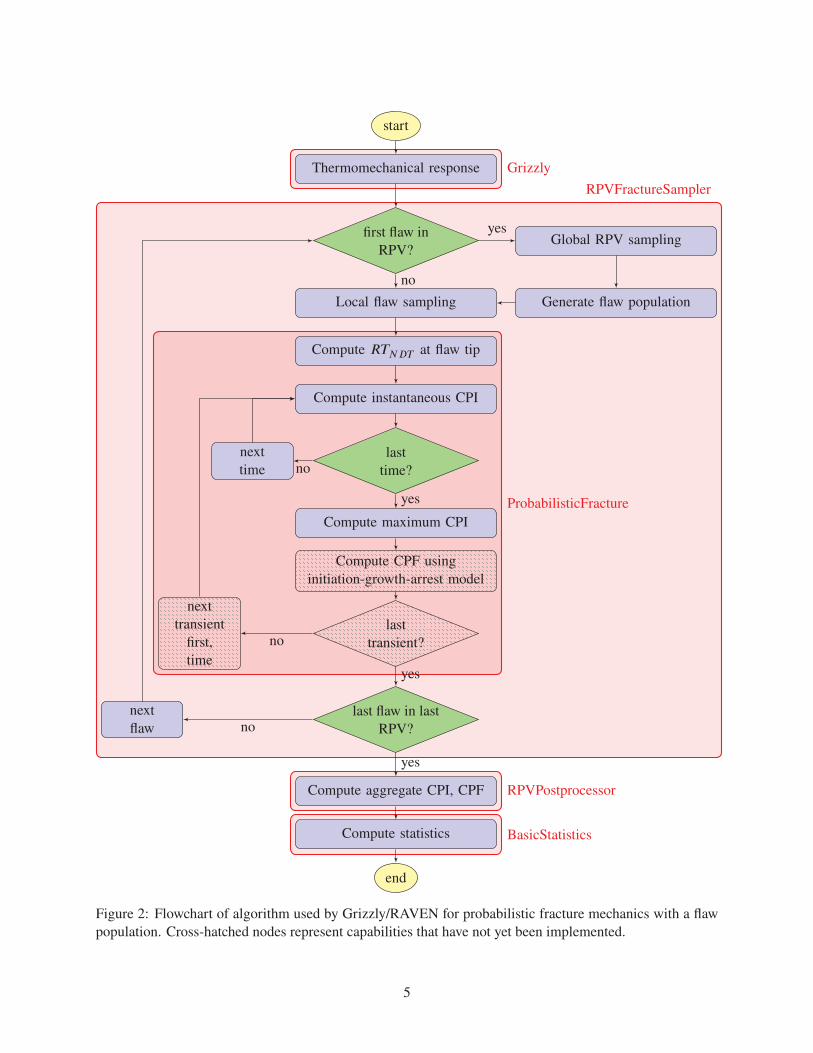
2.1.2 Grizzly/RAVEN implementationThe goal of the present work was to replicate as closely as possible the PFM methodology used by FA-

VOR using the Grizzly and RAVEN codes. Figure 2 shows a flowchart of the algorithm as implemented in

Grizzly/RAVEN. The large boxes containing sections of the algorithm indicate the code objects that were

developed to perform these functions. Not all of the features of FAVOR have been implemented in Griz-

zly/RAVEN yet. Notably, the current implementation supports evaluation of only a single transient, and

does not have the initiation-growth-arrest algorithm necessary to compute CPF. The nodes in the flow chart

relating those features are included to indicate how they will fit in this structure, but are cross-hatched to

indicate that they have not yet been implemented.

One of the major challenges that had to be addressed in this implementation was that RAVEN does not

provide a way to nest sampling loops. Because of this, the structure of the sampling had to be modified,

as indicated in Figure 2. The employed sampling strategy flattens out the nested loops into a single loop

over all of the flaws in every RPV realization. When each flaw is evaluated, the full set of input and output

variables associated with that sample and its calculation are stored. An additional output variable that stores

an identifier for the RPV realization that the flaw sample is associated with is stored for each sample. To

compute the aggregate CPI for each RPV, an additional postprocessing step is taken in which all of the

samples for a given RPV realization are assembled based on the RPV realization identifier, and Equation 1

is applied separately to each grouped set of flaws.

In this algorithm, the sampler simply loops through flaws until it reaches the last flaw in the last RPV

realization. The first time a sample is requested, a population of flaws for the first RPV realization is generated

and stored. Subsequent samples are taken from this stored flaw population until the last flaw in that set is used,

and then a new population of flaws is generated and stored for the next RPV. When the flaws are generated

for an RPV, sampling of other variables that are global to an RPV is also performed, and those are stored for

use in the computation of random variables for individual flaws in that RPV.

In addition to describing the flow of the algorithm, Figure 2 also indicates the code modules that are used

to implement its various components. Prior to the PFM phase of the analysis, Grizzly is used to compute the

global thermomechanical response of the RPV. In the current work, this is done using a strip of elements in

a 2D axisymmetric model with appropriate boundary conditions to approximate the behavior of an infinite

cylinder. This is compatible with the approach used by FAVOR, and prior benchmarking has demonstrated

that the two codes produce equivalent results. Grizzly is able to compute this response on a full 2D axisym-

metric or 3D model of the RPV as well. This capability will be used in the future in conjunction with the

PFM capability described here to evaluate scenarios that require higher dimensionality representations of the

RPV.

The RAVEN code is written in the Python language, and is written as an extensible object-oriented

framework. Many of the features of the code are implemented using a combination of base classes (to

define interfaces to functionality) and derived classes (to implement that functionality for specific cases).

3

start

Thermomechanical response

Global RPV sampling

Generate flaw population

Local flaw sampling

Compute 𝑅𝑇𝑁𝐷𝑇 at flaw tip

Compute instantaneous CPI

last time?next

time

Compute maximum CPI

Compute CPF using

initiation-growth-arrest model

last transient?

next

transient,

first

time

last flaw?next

flaw

Compute aggregate CPI, CPF

last RPV?

next

RPV,

first

flaw

Compute statistics

end

yes

yes

yes

yes

no

no

no

no

Figure 1: Flowchart of algorithm used by FAVOR for probabilistic fracture mechanics with a flaw population

4

Grizzly

RPVFractureSampler

ProbabilisticFracture

RPVPostprocessor

BasicStatistics

start

Thermomechanical response

first flaw in

RPV?Global RPV sampling

Generate flaw populationLocal flaw sampling

Compute 𝑅𝑇𝑁𝐷𝑇 at flaw tip

Compute instantaneous CPI

last

time?

next

time

Compute maximum CPI

Compute CPF using

initiation-growth-arrest model

last

transient?

next

transient

first,

time

last flaw in last

RPV?

next

flaw

Compute aggregate CPI, CPF

Compute statistics

end

no

yes

yes

yes

yes

no

no

no

Figure 2: Flowchart of algorithm used by Grizzly/RAVEN for probabilistic fracture mechanics with a flaw

population. Cross-hatched nodes represent capabilities that have not yet been implemented.

5

The capability described here was implemented using three specialized inherited classes that extend the base

functionality of RAVEN for the RPV PFM application.

The sampling algorithm is implemented using a Python class called RPVFractureSampler that derives

from the base Sampler class in RAVEN. This class provides all of the functionality needed to generate the

flaw samples with all of the associated random variables based on the methodology used by FAVOR. It

generates the flaw population for each RPV realization, including geometric characteristics and assignment

of flaws to major regions in the vessel and appropriate sampling of steel chemistry variables.

The RPVFractureSampler offers flexibility in the ways that flaws can be defined. It can generate the flaw

population using sampling based on distributions of flaw geometric characteristics. It alternatively allows

for the geometric characteristics of each individual flaw to be read in from a text file containing that data

formatted as a comma-separated table. This can be useful for evaluating scenarios where the flaw population

is known. Alternatively, PFM analyses can be performed without using RPVFractureSampler at all. Any

of the other Sampler classes in RAVEN can be used as long as the appropriate set of variables defining

the flaws is defined. For instance, the CustomSampler can be used to read in a comma-separated text table

containing the full set of parameters for a set of flaws, including flaw geometry and chemistry parameters.

This can be very useful for debugging and benchmarking purposes to compute the CPI for specific flaws with

specific parameters.

Most of the specialized classes developed for this capability are maintained in the Grizzly code reposi-

tory. RAVEN currently provides application programming interfaces (APIs) that allow users to write custom

classes that derive from many of the base classes, and the code for these classes can exist in another loca-

tion than the RAVEN code directory structure. Such support does not currently exist for the Sampler class.

As a result, the code must currently be implemented in the RAVEN code directory structure. Because this

capability is specific for RPV analysis, it cannot be distributed with the rest of the RAVEN code base, so

it currently exists in a development version of RAVEN that is not distributed. There are plans to develop

an API to permit users to extend the Sampler class. This code will be added to the Grizzly code base for

distribution with Grizzly at that time.

All calculations needed to compute CPI for a given flaw are done in the ProbabilisticFracturemodule, which is implemented as a RAVEN ExternalModel. This code computes the ductile to brittle

transition temperature, 𝑅𝑇𝑁𝐷𝑇 for a specific flaw using the EONY model [4]. It then uses a reduced order

model to compute the 𝐾𝐼 history of the flaw, as described in detail in Section 2.5. An early version of the

ProbabilisticFracture module was described in [5]. That initial version required a 𝐾𝐼 history as input.

For the present work, this module was extended to allow for it to either internally compute 𝐾𝐼 histories for

embedded and surface-breaking flaws using reduced order models, or read them in from a file.

Finally, the RPVPostprocessor module was developed to compute the aggregate CPI for the set of flaws

associated with an RPV. This class, which derives from the Postprocessor base class in RAVEN, takes

the set of inputs and outputs for all flaws, and generates as output a smaller array of aggregate CPIs for each

RPV realization.

2.2 Flaw Geometry SamplingThe flaw populations in FAVOR are generated using files that define a set of distributions of flaw density,

depth, and aspect ratio. These files are generated using the VFLAW tool developed by Pacific Northwest

National Laboratory as part of the NRC’s PTS Re-Evaluation Project [6]. To facilitate the use of the tools

under development with existing plant-specific data, they have a capability to generate flaw distributions

based on files formatted by that tool in the same manner as is done in FAVOR.

These flaw population characterization files contain a set of 1000 tables of data, each of which is a

unique distribution of the flaw population. These distributions define the density of flaws of a given through-

thickness dimension, and for each dimension bin also define the distribution of the aspect ratio of flaws

6

having that dimension. In a PFM analysis, the first 1000 RPV realizations use the first 1000 flaw distributions

sequentially, after which a counter is reset, and the flaw distributions are re-used in sequence.

Three separate files are used to define distributions of embedded flaws in plates and welds, and surface

breaking flaws (which can be in either plate or weld regions). The generated flaws can be oriented in either the

axial or circumferential orientations. In plate regions, the embedded flaws have equal probabilities of having

axial or circumferential orientations. In weld regions, embedded flaws are oriented to align with the weld

orientation. Inner surface-breaking flaws are all assumed to be in the circumferential orientation because of

the process of applying the cladding, while outer surface-breaking flaw orientations are determined in the

same manner as described above for embedded flaws.

The information stored about each flaw consists of the following data, all stored as variables in RAVEN:

• depth_inner: The depth of the innermost point of the flaw (zero for surface-breaking flaws)

• depth_outer: The depth of the outermost point of the flaw

• aspect_ratio: The aspect ratio of the flaw

• orientation: Flag denoting whether the flaw is axially or circumferentially oriented

2.3 Chemistry SamplingThe content of the alloying elements Cu, Ni, Mn and P is sampled, and the sampled contents are used as

input in the EONY embrittlement correlation. The sampling scheme follows that in FAVOR and is outlined

in this section.

The user provides the following input:

• For each subregion: best estimates in weight% of the chemistry content: Cusubr, Nisubr, Mnsubr, Psubr

• Standard deviations of normal distributions for weld chemistry content: 𝜎Cu,RPV, 𝜎Ni,RPV, 𝜎Mn,RPV,

𝜎P,RPV

• Standard deviations of normal distributions for plate chemistry content: 𝜎Cu,RPV, 𝜎Ni,RPV, 𝜎Mn,RPV,

𝜎P,RPV

For each RPV realization, the global standard deviation of Mn in plates or forgings is sampled.

𝜎Mn,RPV ←

{Weibull(0, 0.06933, 2.4708) wt% in plates

JohnsonSB(0.00163, 0.03681, 0.83358, 1.15153) wt% in forgings

For each subregion of the RPV realization, the global subregion chemistry content is sampled. For plate

and forging subregions, the content is sampled from normal distributions defined by the best estimate means

and standard deviations input by the user.

Cusubr ← (Cusubr, 𝜎Cu,RPV)

Nisubr ← (Nisubr, 𝜎Ni,RPV)

Mnsubr ← (Mnsubr, 𝜎Mn,RPV)

Psubr ← (Psubr, 𝜎P,RPV)

7

For weld subregions, the standard deviations of the normal distributions for Cu, Ni and Mn are sampled

from specific normal distributions. The subregion chemistry content is then sampled from normal distribu-

tions defined by the best estimate means and the sampled standard deviations.

𝜎Cu ← (0.167 × Cusubr,min(0.0718 × Cusubr, 0.0185))𝜎Ni ← (0.029, 0.0165)𝜎Mn ← Weibull(0.01733, 0.04237, 1.83723)

Cusubr ← (Cusubr, 𝜎Cu,subr)

Nisubr ← (Nisubr, 𝜎Ni,subr)

Mnsubr ← (Mnsubr, 𝜎Mn,subr)

Psubr ← (Psubr, 𝜎P,subr)

For each flaw, the local chemistry is calculated as the sum of the global chemistry and a small local

variability. Mn has a larger local variability and is sampled from a normal distribution.

Cuflaw = Cusubr + ΔCu

Niflaw = Nisubr + ΔNi

Mnflaw = (Mnsubr, 𝜎Mn)

Pflaw = Psubr + ΔP

For plates, the local variability is calculated by:

ΔCu ← Logistic(−3.89 × 10−7, 0.00191)

ΔNi ← Logistic(−1.39 × 10−7, 0.00678)

ΔP ← Logistic(1.3 × 10−5, 0.000286)𝜎Mn ← JohnsonSB(0.00163, 0.03681, 0.83358, 1.15153)

For welds, the local variability is calculated by:

ΔCu ← Logistic(6.85 × 10−8, 0.0072)

ΔNi ← Logistic(−0.0014, 0.00647)

ΔP ← Logistic(3.27 × 10−6, 0.000449)𝜎Mn ← JohnsonSB(0.00163, 0.03681, 0.83358, 1.15153)

2.4 RTNDT SamplingThe transition temperature RTNDT characterizes the irradiation-induced embrittlement of the RPV steel. The

shift in RTNDT, ΔRTNDT, compared to the unirradiated value, RTNDT(0), is estimated using the EONY model

8

based on the sampled chemistry content of the steel and the neutron fluence at the depth of the flaw [7].

RTNDT for each flaw is calculated using the formula:

𝑅𝑇NDT = 𝑅𝑇 NDT(0) − 𝑅𝑇 epistemic + Δ𝑅𝑇 NDT (2)

The epistemic uncertainty, RTepistemic is included to account for the difference between values of RTNDT

and T0 estimated directly from fracture toughness data using the Master Curve method [3]. The magnitude

of RTepistemic is sampled once for each subregion of an RPV realization from a distribution given by:

𝑅𝑇 epistemic = Weibull(−29.5, 78.0, 1.73) (3)

For each flaw,𝑅𝑇 NDT(0) is sampled from a normal distribution defined by the mean RTNDT(0) and standard

deviation 𝜎𝑅𝑇NDT(0)of the subregion (input by the user).

𝑅𝑇 NDT(0) = (𝑅𝑇NDT(0), 𝜎𝑅𝑇NDT(0)) (4)

2.5 Failure ComputationTo compute the probability of failure of a flaw with given geometric and chemistry characteristics requires

that the embrittlement be characterized, and then that the history of 𝐾𝐼 be computed. Once these are avail-

able, the CPI can be computed using a temperature-dependent Weibull distribution. The embrittlement is

currently computed using the EONY model [4], which is based on data obtained from surveillance speci-

mens, and is valid for the range of irradiation exposure observed in the current nuclear reactor fleet.

In general, computation of the stress intensity factor for a flaw can be a computationally expensive pro-

cess. It can be computed for a specific flaw geometry and loading condition using a detailed 3D finite element

model. Because of the large number of flaws that must be evaluated, it is not practical to run such models

for each flaw sample, so reduced order models (ROMs) to represent 𝐾𝐼 as a function of flaw geometry and

loading are employed. The ROMs used in the current work to compute stress intensity factors for surface-

breaking and embedded flaws described in the following sections.

These are the same procedures used by the FAVOR code. There has also been work underway, as doc-

umented in [8], to evaluate a variety of surrogate modeling techniques to automatically generate ROMS for

fracture mechanics models. This work has demonstrated promising results, and is planned to be applied to

consider flaw geometries not represented by the current ROMS for axis-aligned flaws.

2.5.1 Surface-breaking Flaw 𝐾𝐼 CalculationStress Intensity Factor Influence Coefficient Procedure The method used for deterministic analyses of

circumferential or axial inner surface breaking elliptical flaws in the presence of cladding for mode 𝐼 loading

represents the combined effects of stresses in the base metal and cladding on 𝐾𝐼 :

𝐾𝐼 = 𝐾𝐼𝑏𝑎𝑠𝑒+𝐾𝐼𝑐𝑙𝑎𝑑

(5)

where the stress intensity factor solution for a given flaw is found by calculating the stress intensity factors for

the base material (𝐾𝐼𝑏𝑎𝑠𝑒) and cladding (𝐾𝐼𝑐𝑙𝑎𝑑

) individually. The individual 𝐾𝐼 values are calculated using

the principle of linear superposition discussed in [9].

The method for obtaining the stress intensity factor for the base material requires the complete RPV

through-wall stress distribution described by a cubic polynomial as well as a set of coefficients called Stress

Intensity Factor Influence Coefficients (SIFICs). These components are combined in the following equation

and used to determine the stress intensity factor for the base metal:

9

𝐾𝐼𝑏𝑎𝑠𝑒=

3∑𝑖=0

𝐶𝑗𝐾𝑗

√𝜋𝑎 (6)

In Equation 6, 𝑎 is the flaw depth, 𝐾𝑗 are the SIFICs, and 𝐶𝑗 are the coefficients to the polynomial used

to describe the through-wall stress distribution in the base material. The function weights are obtained using

a least squares polynomial fit, shown in Equation 7:

𝜎

(𝑎′

𝑎

)= 𝐶0 + 𝐶1

(𝑎′

𝑎

)+ 𝐶2

(𝑎′

𝑎

)2+ 𝐶3

(𝑎′

𝑎

)3(7)

The SIFICs for the base material used in equation 6 are obtained through finite element models for specific

flaw geometries, and curve-fitting techniques can used to obtain these for other flaw geometries. Each SIFIC

for the base metal is determined as a function of the RPV’s wall thickness relative to its inner radius (𝑅∕𝑡),the relative flaw depth (𝑎∕𝑡) and the flaw aspect ratio (𝐿∕𝑎). The appropriate SIFICs are determined based

upon the provided RPV and flaw geometry using a library of previously determined solutions. After the

stress polynomial coefficients and corresponding SIFICs have been determined, the base metal component

of equation 6 can be determined using Equation 7.

It is important to recall that this analysis is for a transient process. Therefore the global RPV finite element

model is subjected to boundary conditions that vary over time, and is evaluated at each time step specified in

the sequence. This means that at each time step in the simulation, the stresses at each of the radial positions

will change. The SIFICs, however, are constant through the transient simulation because they are a function

only of geometry. Thus, the coefficients in equation 7 must be determined and stored for every time step in

the simulation. Additionally, new coefficients must be determined for every flaw length that is considered in

each deterministic analysis. This is shown by Equation 7, where 𝑎′ is a radial distance spanning from zero

to a, which is the depth of the flaw being evaluated in the deterministic analysis. Because the polynomial

is fit over the length of the flaw being considered, the polynomial must be determined for each flaw that is

analyzed. This process can be repeated for any flaw length, 𝑎, such that the value is contained within the

domain of SIFIC data.

The SIFICs for the base metal are independent of cladding effects, and the contributions of base metal

and cladding are linearly superimposed. The stress intensity factor for the cladding is determined through

the application of the weighting function similar to the method described for the base metal calculation.

The cladding function weights require the coefficients from two separate linear polynomials. The first is

a linear least squares fit of the stresses in the cladding as a function of the corresponding radial positions.

This polynomial is fit over the full thickness of the cladding material and is not related to crack depth. The

resulting polynomial is described by two coefficients, which will be referred to as the actual coefficients.

The second set of coefficients is obtained by extrapolating a line through the thickness of the cladding using

the two inner-most stress values located within the base material. The final coefficients used as the function

weights in equation 8 are obtained by subtracting the extrapolated coefficients from the actual coefficients.

𝐾𝐼𝑐𝑙𝑎𝑑=

1∑𝑖=0

𝐶𝑗𝐾𝑗

√𝜋𝑎 (8)

Once the coefficients for the cladding have been determined, the appropriate SIFICs can be selected and

used in Equation 8 to determine the stress intensity factor for the cladding. These values are parameterized

using the same geometric characteristics used in the base metal SIFICs, in addition to a cladding thickness

parameter. The appropriate values are determined using interpolation within a dataset of pre-determined

finite element solutions provided in the FAVOR Theory and Implementation Manual. The final result can

10

then be determined using equation 5, where the base metal and cladding stress intensity factors are summed,

resulting in the total stress intensity factor for the flaw of interest.

A3000 module Earlier versions of FAVOR computed the SIFICs using the procedure described above by

interpolation between values obtained from finite element solutions of specific flaw geometries. A new pro-

cedure was implemented in FAVOR that uses closed form expressions for SIFICs as documented in section

A3000 of the ASME Boiler and Pressure Vessel Code. ORNL developed a Python module that incorporates

implementation of ASME A3000 curve fits for the stress-intensity-factor influence coefficients (SIFIC) in-

ternal finite and infinite flaws with axial and circumferential orientations for RPV base material. The latter

module is a Python implementation of the FAVOR capability already included in FAVOR since v. 15.3 [10].

The latter module was originally implemented in the Fortran language. ORNL transmitted this code to INL

for integration into Grizzly.

For finite-length surface breaking flaws, revised SIFIC(s) provide consistency in the normalized flaw

depths used in the databases for nominal 𝑅𝑖∕𝑡 values of 10 and 20. Specifically, in the tables for 𝑅𝑖∕𝑡 = 20,

SIFICs are now given for the second relative flaw depth at 𝑎∕𝑡 = 0.0184 (see Table B37 [10]); the latter

relative flaw depth at the second position in the tabulation for 𝑅𝑖∕𝑡 = 20 now matches that for 𝑅𝑖∕𝑡 = 10 at

the second position (see Table B2 [10]). In the original SIFIC tables, the relative flaw-depth values of 𝑎∕𝑡for 𝑅𝑖∕𝑡 = 10 and 20 differ only in the second normalized flaw depth position in the tabulations (see Tables

B2 and B11 [10]). The foregoing change was made to simplify interpolation of applied 𝐾𝐼 factors for those

intermediate values of 𝑅𝑖∕𝑡 between 10 and 20, and to correct an error found in previous versions of FAVOR.

For infinite axial and 360°continuous circumferential internal surface-breaking flaws, the entire database

of SIFICs was regenerated using the same scheme employed for finite-length, semielliptical internal surface-

breaking flaws (see Section 5.1.3.2 [10] for a detailed description of that methodology which explicitly mod-

els the clad layer); the revised SIFIC database is given in Tables B38-B41 [10]. This change from previous

versions of FAVOR was made to address issues identified for very shallow flaws where the effects of the

cladding layer play a more significant role than is the case with deeper flaws. The motivation for this change

is due to the fact that the original SIFIC database for infinite axial and 360°continuous circumferential in-

ternal surface-breaking flaws was generated in the early 1980s using a technique (see Section 5.1.3.2 [10])

that did not explicitly account for the effects of cladding. The revised SIFIC database now includes cladding

effects consistent with the technique used for finite-length flaws.

2.5.2 Embedded Flaw 𝐾𝐼 CalculationThe method for calculating Mode I stress intensity factors for embedded flaws follows that in [11], as pre-

sented in the FAVOR Theory Manual. It is based on resolving the applied stress field through the wall into the

linear superposition of approximate membrane and bending stress components. The membrane and bend-

ing stress components are obtained by fitting a straight line through the stresses at the two crack tips and

recording the value at the midpoint through the wall and at the (outer or inner) surface, respectively.

𝜎𝑚 = ��(𝑡∕2) =𝜎(𝑥2) − 𝜎(𝑥1)

2𝑎× (𝑡∕2 − 𝑥1) + 𝜎(𝑥1) (9)

𝜎𝑏 = ��(0) − 𝜎𝑚 =𝜎(𝑥1) − 𝜎(𝑥2)

2𝑎× (𝑡∕2) (10)

The stress intensity factor, KI, is computed as a linear superposition of the membrane and bending stress

components using the relation:

𝐾𝐼 = (𝑀𝑚𝜎𝑚 +𝑀𝑏𝜎𝑏)√𝜋𝑎∕𝑄, (11)

11

where

2𝑎 = the minor axis of the elliptical subsurface flaw (12)

𝑄 = flaw shape parameter (13)

𝑀𝑚 = free-surface correction factor for membrane stress (14)

𝑀𝑏 = free-surface correction factor for bending stress (15)

𝜎𝑚 = membrane stress (16)

𝜎𝑏 = bending stress (17)

The shape factor, 𝑄, is given by the complete elliptic integral of the second kind:

𝑄(𝑥) = 𝐸2(𝑥) (18)

𝐸(𝑥) = ∫𝜋∕2

0

√1 − 𝑥 sin2 𝜃𝑑𝜃 for 0 ≤ 𝑥 ≤ 1 (19)

𝑥 = 1 − 4(𝑎

𝐿

)2(20)

The free-surface correction factors for membrane stress and bending stress are defined in equations 21

and 22, respectively. In these equations, 𝑎 is half of the flaw length in the radial direction and 𝑒 is the distance

between the midpoint through the wall and the midpoint of the flaw.

𝑀𝑚 = 𝐷1 +𝐷2(2𝑎∕𝑡)2 +𝐷3(2𝑎∕𝑡)4 +𝐷4(2𝑎∕𝑡)6 +𝐷5(2𝑎∕𝑡)8 +𝐷6(2𝑎∕𝑡)20[

1 − (2𝑒∕𝑡) − (2𝑎∕𝑡)]1∕2 (21)

where:

𝐷1 = 1𝐷2 = 0.5948𝐷3 = 1.9502(𝑒∕𝑎)2 + 0.7816(𝑒∕𝑎) + 0.4812𝐷4 = 3.1913(𝑒∕𝑎)4 + 1.6206(𝑒∕𝑎)3 + 1.8806(𝑒∕𝑎)2 + 0.4207(𝑒∕𝑎) + 0.3963𝐷5 = 6.8410(𝑒∕𝑎)6 + 3.6902(𝑒∕𝑎)5 + 2.7301(𝑒∕𝑎)4 + 1.4472(𝑒∕𝑎)3 + 1.8104(𝑒∕𝑎)2 + 0.3199(𝑒∕𝑎) + 0.3354𝐷6 = 0.303

𝑀𝑏 = 𝐸1 +𝐴[

1 − (2𝑒∕𝑡) − (2𝑎∕𝑡)]1∕2 (22)

𝐴 = 𝐸2(2𝑒∕𝑡) + 𝐸3(2𝑒∕𝑡)2 + 𝐸4(2𝑒∕𝑡)(2𝑎∕𝑡) + 𝐸5(2𝑎∕𝑡)(2𝑒∕𝑡)2 + 𝐸6(2𝑎∕𝑡) + 𝐸7(2𝑎∕𝑡)2

+ 𝐸8(2𝑒∕𝑡)(2𝑎∕𝑡)2 + 𝐸9

where:

𝐸1 = 0.8408685 𝐸2 = 1.509002 𝐸3 = −0.603778𝐸4 = −0.7731469 𝐸5 = 0.1294097 𝐸6 = 0.8841685𝐸7 = −0.07410377 𝐸8 = 0.04428577 𝐸9 = −0.8338377

12

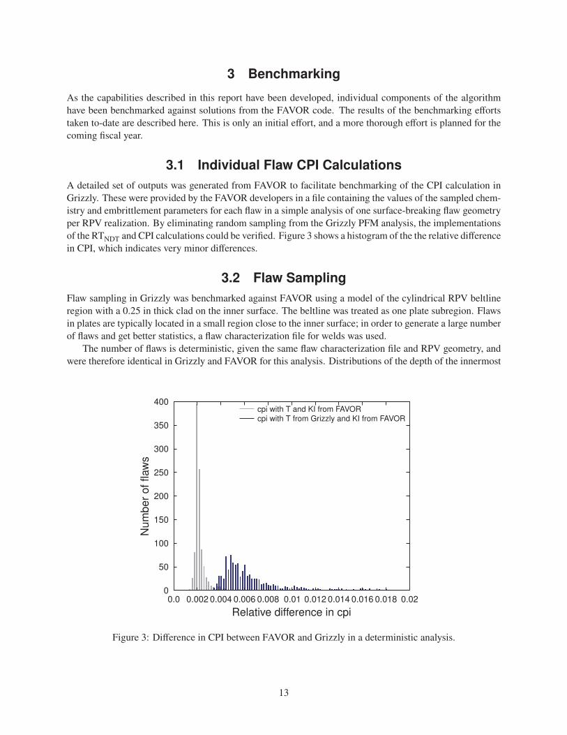
3 Benchmarking

As the capabilities described in this report have been developed, individual components of the algorithm

have been benchmarked against solutions from the FAVOR code. The results of the benchmarking efforts

taken to-date are described here. This is only an initial effort, and a more thorough effort is planned for the

coming fiscal year.

3.1 Individual Flaw CPI CalculationsA detailed set of outputs was generated from FAVOR to facilitate benchmarking of the CPI calculation in

Grizzly. These were provided by the FAVOR developers in a file containing the values of the sampled chem-

istry and embrittlement parameters for each flaw in a simple analysis of one surface-breaking flaw geometry

per RPV realization. By eliminating random sampling from the Grizzly PFM analysis, the implementations

of the RTNDT and CPI calculations could be verified. Figure 3 shows a histogram of the the relative difference

in CPI, which indicates very minor differences.

3.2 Flaw SamplingFlaw sampling in Grizzly was benchmarked against FAVOR using a model of the cylindrical RPV beltline

region with a 0.25 in thick clad on the inner surface. The beltline was treated as one plate subregion. Flaws

in plates are typically located in a small region close to the inner surface; in order to generate a large number

of flaws and get better statistics, a flaw characterization file for welds was used.

The number of flaws is deterministic, given the same flaw characterization file and RPV geometry, and

were therefore identical in Grizzly and FAVOR for this analysis. Distributions of the depth of the innermost

0

50

100

150

200

250

300

350

400

Num

ber

offla

ws

0.0 0.002 0.004 0.006 0.008 0.01 0.012 0.014 0.016 0.018 0.02

Relative difference in cpi

cpi with T and KI from FAVORcpi with T from Grizzly and KI from FAVOR

Figure 3: Difference in CPI between FAVOR and Grizzly in a deterministic analysis.

13

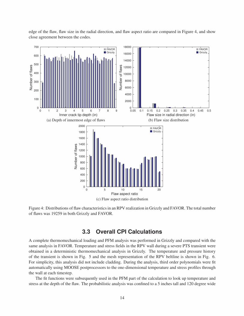
edge of the flaw, flaw size in the radial direction, and flaw aspect ratio are compared in Figure 4, and show

close agreement between the codes.

0

100

200

300

400

500

600

700

Num

ber

offla

ws

0 1 2 3 4 5 6 7 8 9

Inner crack tip depth (in)

FAVORGrizzly

(a) Depth of innermost edge of flaws

0

2000

4000

6000

8000

10000

12000

14000

16000

18000

Num

ber

offla

ws

0.05 0.1 0.15 0.2 0.25 0.3 0.35 0.4 0.45 0.5

Flaw size in radial direction (in)

FAVORGrizzly

(b) Flaw size distribution

0

200

400

600

800

1000

1200

1400

1600

1800

2000

Num

ber

offla

ws

0 5 10 15 20

Flaw aspect ratio

FAVORGrizzly

(c) Flaw aspect ratio distribution

Figure 4: Distributions of flaw characteristics in an RPV realization in Grizzly and FAVOR. The total number

of flaws was 19259 in both Grizzly and FAVOR.

3.3 Overall CPI CalculationsA complete thermomechanical loading and PFM analysis was performed in Grizzly and compared with the

same analysis in FAVOR. Temperature and stress fields in the RPV wall during a severe PTS transient were

obtained in a deterministic thermomechanical analysis in Grizzly. The temperature and pressure history

of the transient is shown in Fig. 5 and the mesh representation of the RPV beltline is shown in Fig. 6.

For simplicity, this analysis did not include cladding. During the analysis, third order polynomials were fit

automatically using MOOSE postprocessors to the one-dimensional temperature and stress profiles through

the wall at each timestep.

The fit functions were subsequently used in the PFM part of the calculation to look up temperature and

stress at the depth of the flaw. The probabilistic analysis was confined to a 5 inches tall and 120 degree wide

14

300

350

400

450

500

550

600

Tem

pera

ture

(K)

0

2

4

6

8

10

12

14

16

18

20

Pre

ssur

e(M

Pa)

0 2000 4000 6000 8000 10000 12000 14000 16000

Time (s)

Figure 5: Time histories of coolant temperature and pressure applied as boundary conditions to 2D strip

model of RPV beltline region.

section of the beltline region. The average number of flaws in this region over 1000 RPV realizations was

111.6. In Grizzly, 2.4% of flaws had a CPI larger than zero, while for FAVOR that number was 2.2%. The

average CPI over the 1000 RPV realizations was 0.01835 in FAVOR and 0.00134 in Grizzly.

The sources of this discrepancy in the results are still under investigation. Many of the components of

the analysis have been checked and compare well with FAVOR, but there are still more components of the

algorithm that need to be checked individually against FAVOR to ensure that they are in agreement.

The distributions of RTNDT from Grizzly and FAVOR for flaws in 100 RPV realizations are compared

in Fig. 7. The results generally agree well, except for the tails of the distributions at very low transition

temperatures. The difference may be due to subtle differences in the sampling procedures and needs to be

investigated further.

15

�

Figure 6: Cutaway of representative RPV (left), and finite element mesh (right) used to represent the beltline

region using a 2D strip model. The inner radius of the wall is 86 in and the wall thickness is 8.75 in.

Figure 7: Comparison of RTNDT distributions in the same plate analysis in Grizzly and FAVOR.

16

4 Summary and Future Development

4.1 Summary of Current DevelopmentsThis report documents work to develop and perform initial testing of a capability to perform PFM analyses

of an RPV containing a population of flaws. The following code developments were made in support of this

work:

• A specialized sampling module that mimics the two-level sampling strategy used by FAVOR was

developed.

• A capability to generate populations of flaws based on probabilistic descriptions of flaw geometry from

the VFLAW code was developed.

• A capability to generate samples of RPV steel chemistry parameters was developed.

• Code modules to use ROMs to compute 𝐾𝐼 for embedded and surface-breaking flaws were developed.

• Initial benchmarking of these newly developed code modules against FAVOR solutions was performed.

4.2 Planned future workThe following developments are planned to develop a complete PFM capability:

• More thorough benchmarking of individual components and the capability in its entirety will be per-

formed against the FAVOR code, and issues will be resolved.

• Missing capabilities currently available in FAVOR will be implemented. These include the following:

– An ability to compute CPF in addition to CPI

– An ability to evaluate multiple transients

• The entire capability documented here will be made available in the Grizzly code base after an API is

developed for Sampler classes in RAVEN.

• An ability to integrate higher-dimensionality models for the global response of RPVs with these PFM

algorithms will be developed.

• An ability to use ROMs to rapidly compute fracture parameters for flaw geometries that cannot cur-

rently be evaluated will be developed.

4.3 Benefits of this approachWhen complete, the RAVEN/Grizzly approach being developed will provide the following benefits for prob-

abilistic fracture analysis of RPVs under transient conditions:

• Grizzly and RAVEN are both built on modern, flexible code infrastructures that provide many basic

facilities that are leveraged for this specific application.

• RAVEN provides advanced techniques that can greatly speed up the process of probabilistic fracture

analysis, including adaptive sampling techniques and parallel processing.

17

• The 2D and 3D capabilities provided by Grizzly can be used to represent local nonuniformities in the

global reactor pressure vessel response, such as local geometric effects and effects introduced by a

nonuniform thermal environment.

• The reduced order model capability being developed in Grizzly will permit automated generation of

models that can be rapidly evaluated for a wide variety of flaw configurations.

18

5 References

1. B. Spencer, M. Backman, P. Chakraborty, and W. Hoffman, Reactor Pressure Vessel Fracture AnalysisCapabilities in Grizzly, INL/EXT-15-34736, Idaho National Laboratory, Idaho Falls, ID, Mar. 2015.

2. T. Dickson, P. T. Williams, and S. Yin, Fracture Analysis of Vessels – Oak Ridge, FAVOR, v12.1,Computer Code: User’s Guide, ORNL/TM-2012/566, USNRC Adams number ML13008A016, Oak

Ridge National Laboratory, Oak Ridge, TN, Nov. 2012.

3. P. Williams, T. Dickson, and S. Yin, Fracture Analysis of Vessels – Oak Ridge, FAVOR, v12.1, ComputerCode: Theory and Implementation of Algorithms, Methods, and Correlations, ORNL/TM-2012/567,

USNRC Adams number ML13008A015, Oak Ridge National Laboratory, Oak Ridge, TN, Nov. 2012.

4. E. Eason, G. Odette, R. Nanstad, and T. Yamamoto, “A physically-based correlation of irradiation-

induced transition temperature shifts for RPV steels”, Journal of Nuclear Materials, vol. 433, no. 1-3,

pp. 240–254, Feb. 2013.

5. B. Spencer, W. Hoffman, S. Sen, C. Rabiti, T. Dickson, and R. Bass, Initial Probabilistic Evaluationof Reactor Pressure Vessel Fracture with Grizzly and RAVEN, INL/EXT-15-37121, Idaho National

Laboratory, Idaho Falls, ID, Oct. 2015.

6. F. A. Simonen, S. R. Doctor, G. J. Schuster, and P. G. Heasler, A Generalized Procedure for Gener-ating Flaw-Related Inputs for the FAVOR code, NUREG/CR-6817, PNNL-14268, Pacific Northwest

National Laboratory, Richland, WA, Mar. 2004.

7. B. Spencer, J. Busby, R. Martineau, and B. Wirth, A Proof of Concept: Grizzly, the LWRS ProgramMaterials Aging and Degradation Pathway Main Simulation Tool, Idaho National Laboratory, Idaho

Falls, ID, 2012.

8. W. M. Hoffman, M. E. Riley, and B. W. Spencer, “Surrogate Model Development and Validation for

Reliability Analysis of Reactor Pressure Vessels”, ASME Pressure Vessels and Piping Conference,

PVP2016-63341, Vancouver, BC, Canada, July 2016.

9. H. F. Bückner, “A Novel Principle for the Computation of Stress Intensity Factors”, Z. angew. Math.Mech. Vol. 50, pp. 529–546, 1970.

10. P. Williams, T. L. Dickson, S. Yin, and B. R. Bass, Fracture Analysis of Vessels – Oak Ridge, FA-VOR, v15.3, Computer Code: Theory and Implementation of Algorithms, Methods, and Correlations,

ORNL/LTR-2016/71, ORNL/TM-2016/61454, Oak Ridge National Laboratory, Oak Ridge, TN, 2015.

11. R. C. Cipolla, Computational Method to Perform the Flaw Evaluation Procedure as Specified in theASME Code, Section XI, Appendix A, EPRI Report NP-1181, Failure Analysis Associates, Sept. 1979.

19