innovation-adjusted economic complexity and growth: · pdf fileand descriptive approach to...
TRANSCRIPT
Innovation-adjusted Economic Complexity and Growth:Does product-specific patenting reveal enhanced economic
capabilities?∗
Mingzhi XuUniversity of California, Davis
Travis J. LybbertUniversity of California, Davis
October 5, 2017
Abstract
To understand the economic growth has been a primary pursuit for generations ofeconomists. Hidalgo and Hausmann (2009) charted new territory in this pursuit by usingbipartite international trade networks to characterize the economic complexity of a coun-try based on the capabilities implied by the products it exports. The resulting EconomicComplexity Index (ECI) correlates strongly with income levels and predicts subsequenteconomic growth with some statistical precision. We propose an Innovation-adjusted ECI(i-ECI) that uses a high-resolution patent-trade concordance to construct trade networksweighted by domestic and international patent application flows. The i-ECI thereby re-flects firms’ decisions about where to seek patent protection on industry-specific inven-tions, allows for heterogeneity in the relative importance of patenting across industries,and implicitly captures firms’ perceived innovation potential in the recipient countries.Although the i-ECI is highly correlated with the ECI (correlation coefficient>92%), it is astronger and more statistically precise predictor of economic growth than the unadjustedECI.
∗Xu: Economics, University of California, Davis ([email protected]); Lybbert: Agricultural and Resource Economics,University of California, Davis ([email protected]).
1

1 Introduction
Understanding the drivers and dynamics of economic growth has long been a central theme of eco-
nomics and a common obsession among micro- and macro-economists alike. Economists’ pursuit
of the social, technical and institutional complexities that generate productivity gains and aggre-
gate economic growth was first philosophical, then mathematical and – most recently – predomi-
nantly empirical. In recent decades, the confluence of data availability, econometric techniques and
computing power have brought powerful empirical perspectives to fundamental economic growth
questions. In this vein, Hidalgo and Hausmann (2009) propose an intriguing approach that lever-
ages bipartite international trade networks to characterizing and understanding economic complex-
ity. The Economic Complexity Index (ECI) they construct based on trade networks are strongly
correlated with income. More encouraging still, economic complexity measures in a baseline pe-
riod predict subsequent economic growth. We build on this novel empirical approach by weaving
product-specific patent application flows into these international trade networks and find that ad-
justing the ECI to reflect firms’ perceptions of the innovation potential in a given economy improves
its predictive power for subsequent economic growth.
Hidalgo and Hausmann (2009)explain their economic complexity approach using a metaphor of
a bucket of Legos: With more and more diverse Lego blocks, a child can build more elaborate Lego
models. Each distinct Lego block in this metaphor represents an economic capability. They then
ask, can we “infer properties such as the diversity and exclusivity of the Lego pieces inside a child’s
bucket by looking only at the models that a group of children, each with a different budget of Le-
gos, can make”? (p.10570) They propose a method of leveraging international trade data to infer the
underlying capabilities possessed by a given country that enable the production patterns evident in
these data. In their words, “connections between countries and products signal the availability of
capabilities in a country just like the creation of a model by a child signals the availability of specific
set of Lego pieces.” (p10570). This proposed approach is the basis for the ECI. While this data-driven
and descriptive approach to characterizing economic complexity neither attempts to explain mecha-
nisms that lead to the accumulation of such capabilities nor postulates the dynamic interrelationships
between characteristics of an economy of these production capabilities, the approach is consistent
with both conceptual and more rigorous theoretical models of economic growth (see Hausmann and
Hidalgo (2011)).
We extend the construction of the ECI to explicitly account for product-specific innovation in
these international trade networks and explore how the resulting Innovation-adjusted ECI (i-ECI)
may improve our inference of the underlying capabilities that exist in a given economy. Continuing
the metaphor, this adjustment reflects a dimension of Lego blocks beyond their shape and size. Sup-
pose, for example, that blocks come in different colors and brighter colors denote greater innovation
content in a given block. A more brightly colored creation implies more innovative blocks in the
bucket - even if these blocks are the same size and shape of grey blocks in another child’s bucket.
2

Effectively, we ask, “Does the innovation capacity of a given economy represent unique capabilities
that adds to the economic sophistication and complexity of the economy?”
The ECI extracts information from observed patterns of international trade to infer the underly-
ing economic capabilities of countries based on the simple logic that the movement of goods across
borders reflects incentive-compatible decisions of firms based on their knowledge about what can
be produced in a given location. We apply a very similar logic to the observed patterns of product-
specific patenting: Firms choose to seek patent protection in jurisdictions where they perceive strate-
gic value to patent protection. This strategic value reflects firms’ perception of the innovation ca-
pacity of the location. Whether the patent applicant is seeking to produce new goods or services, to
create markets for new products, or to prevent a competitor from gaining a market advantage, the
patenting decision reveals the firms’ assessment of the capabilities of the target country. Note that in
contrast to the ECI, which uses exports from a given country as evidence of economic capabilities, the
i-ECI uses patents received by a country as evidence of firms’ perception of its innovation potential.
While patenting is but one form of innovation and a minor one at that in many sectors, it – like
export data – is readily observable and therefore offers the primary empirical lens into innovation
(CHILICHES (1990)). There are clearly many other dimensions of a country’s innovation capacity
than just the inventions that are patent protected in its jurisdiction, but patent data are widely avail-
able and organized by detailed patent classification systems and therefore provide a logical point
of departure for empirically constructing i-ECI measures. To leverage the high-resolution patent
classification systems and concord patents to trade data organized by industrial classification sys-
tems, we use the ‘algorithmic links with probabilities’ concordance developed by Lybbert and Zolas
(2014). This concordance enables us to weight industry-specific trade flows out of a country by the
corresponding patent flows into the country as the basis for the i-ECI.
Attempts to link the ECI and innovation are not new, most of which consider one as the explana-
tory variable of the other. Among the studies that consider innovation as the factor variables, Sweet
and Maggio (2015) finds that stronger intellectual property rights raises a country’s ECI. Azam (2017)
focuses on the impact of the ECI on national cognitive abilities and innovational output and confirms
a positive relationship between the two. Our research differs from these studies in that we explicitly
integrate patent applications as proxies for innovation capacity into the ECI and explore how the
resulting i-ECI may improve our inference of the underlying capabilities that exist in a given econ-
omy. This analysis relates to another stream of literature that aims to construct new indices to capture
different aspects of the economy. For instance, Ivanova, Strand, Kushnir, and Leydesdorff (2017) pro-
pose an index to reflect the degree of integration between the markets for goods and innovation in
a national innovation systems framework. Donoso (2017) proposes alternative index of innovation
with complexity weights to account for patent quality which is heavily ignored in the previous com-
posite indicators that rely on patent counts.. As a complement to these studies, our index embedded
with patent information aims to explore the role of innovation in affecting an economy’s complexity,
thereby promoting the economic growth, i.e., to what extend, the innovation growth contribute to
3
the economic growth.
The rest of the paper is organized as follows. We introduce our method of constructing i-ECI in
Section 2, and describe our data used in Section 3. Section 4 discusses the empirical results. Lastly,
we conclude in Section 5.
2 Methodology
In this section, we first review the Hidalgo and Hausmann (2009) approach to generating the ECI.
This review, which is not intended to be comprehensive, provides a point of departure for our pro-
posed innovation adjustment. We then describe how we use patent data as the basis of our proposed
i-ECI measure.
2.1 Economic Complexity Index (ECI)
To characterize country and industry 1 complexity, Hidalgo and Hausmann (2009) use the method
of reflection. Following their notation, we denote Mcp as the cp element of the country-product
relationship matrix that captures the structure of trade network such that:
Mcp =
1 if country c is a significant exporter of p
0 otherwise
Country c is regarded as a significant exporter of product p if its Revealed Comparative Advantage
(RCA), which is defined as the export of p as the share of the total export of country c, is greater
than one.2 Formally, if Xcp represents the export of industry p by country c, the RCA of industry p in
country c is expressed as:
RCAcp =Xcp/ ∑p Xcp
∑c Xcp/ ∑c,p Xcp
The intuition behind this definition of RCA is simple: A country that exports more than its ’fair
share’ of total exports for a given industry has a revealed comparative advantage in that industry,
where ’fair share’ is based on the country’s total exports as a share of total global exports. Further,
the elements Mcp can be expressed as:
Mcp =
1 RCAcp > 1
0 otherwise
1The terms product and industry are often used interchangeably in this literature. Note, however, that industry encom-passes both goods and services whereas product refers primarily to goods. Since trade and patent applications typicallycorrespond to products rather than services, we primarily use the term product.
2By adopting one as the ’cutoff value’ we follow the convention in the literature.
4

By construction, Mcp is a matrix with rows indicating different countries and columns different
products. Thus, an element (c, p) is 1 if country c is a significant exporter of product p. Therefore,
we can measure a country’s diversity and a product’s ubiquity by summing over rows and columns
respectively:
Diversityc = kc,0 = ∑p
Mcp
Ubiquityp = kp,0 = ∑c
Mcp
For countries, we calculate the average ubiquity of products that it exports, the average diver-
sity of the countries that make those products and so forth. For products, we calculate the average
diversity of the countries that make them and the average ubiquity of the other products that these
countries make. The calculation can be expressed by the recursion defined as:
kc,N =1
kc,0∑
pMcpkp,N−1 (1)
kp,N =1
kp,0∑
pMcpkc,N−1 (2)
Substituting (1) into (2), we derive:
kc,N =1
kc,0∑
pMcp
1kp,0
∑c′
Mc′pkc′,N−2
= ∑c′
kc′,N−2 ∑Mcp Mc′p
kc,0kp,0(3)
We then define
Mcc′ = ∑p
Mcp Mc′p
kc,0kp,0(4)
Equation (3) can be rewritten as:
kc,N = ∑c′
Mcc′kc′,N−2 (5)
Equation (5) is satisfied when kc,N and kc,N−2 are both one, which corresponds to the eigenvector of
Mcc′ associated with the largest eigenvalue. Since this eigenvector is a vector of ones, which doesn’t
provide information, we instead use the eigenvector associated with the second largest eigenvalue,
which provides the largest variation in the system to measure complexity. Thus, a country’s Eco-
nomic Complexity Index (ECI) is based on normalizing the eigenvector, expressed as:
ECI =~K−Mean(~K)
StdDev(~K)(6)
5
where ~K is the eigenvector of Mcc′ associated with the second largest eigenvalue, Mean(.) denotes
the average and StdDev(.) represents the standard deviation of this eigenvalue.3
With essential features of the construction of the ECI in mind, consider the extent to which inno-
vation enters into this measure of complexity. Clearly, unique economic capabilities - such as those
embodied in a product that is technologically specialized and therefore has very low ubiquity - are to
some degree the result of underlying complexity. Such complexity in the underlying production pro-
cess may demand high levels of innovation. Thus, complexity that is embedded in the ECI already
indirectly and partially reflects the innovative capabilities of countries, but only based on average
differences between industries. If, however, the product-specific ubiquity measures conceal strong
heterogeneity in the innovation capabilities of the industry as it is organized from country to country,
the ECI offers only a muted and incomplete adjustment for innovation capabilities. In practice, this
heterogeneity can be pronounced as the innovation content within a given industry can vary widely
from country to country. For example, HS4 class “Instruments and apparatus for physical or chemi-
cal analysis” (HS4 9027) ranked as the ninth most complex product class in 2014.4 Exports in this class
from some countries are likely to consist of basic equipment, while exports from other countries are
likely to be so much more technologically sophisticated (e.g., with cutting-edge sensors, integrated
software, automated features, high levels of precision, etc.) as to constitute a qualitatively distinct
product class. While the unit value of such equipment might reflect these differences in embedded
technology, the total value of exports in HS4 9027 and therefore the shares of total export value in the
RCA calculation do not. Consequently, the exports in this class from a given country may be more
technologically sophisticated than exports from a different country, but the ECI does not reflect such
qualitative differences. For simplicity and without losing generality, we assume the heterogeneity of
technology sophistication among countries is scaled between zero and unity within industry5, which
depends on both an industry’s general sophistication (up) as well as a country’s capability in adapt-
ing innovation for this given industry (vcp). Country c’s overall capability in applying innovation to
industry p is represented simply as:
ωcp = up × vcp + 1
According to the above expression, a country is more technologically sophisticated in an industry if
the industry itself requires more innovation or the country’s capability in adapting innovation in that
industry is higher. Since the measure is in relative term, for each industry, we assume the referenced
country (the detailed information is provided later) to have zero technology sophistication in the
given industry, (vre fcp = 0) and that the referenced industry to have zero sophistication (ure f
p = 0).
3Analogously, the Product Complexity Index (PCI) is derived as PCI = (~Q − Mean(~Q))/S.D(~Q), where ~Q is theeigenvector of Mpp′ associated with the second largest eigenvalue.
4See http://atlas.cid.harvard.edu/rankings/product/2014/ (accessed 25 April 2017).5In practice, we normalize the industry specific and country-industry specific patent flows in a certain way such that
those two innovation measures are scaled between zero and unity. All that matters is an industry’s relative position in theindustry-innovation ladder, as well as a country’s relative position compared to others within the same industry.
6

There is a yet deeper level of heterogeneity in innovation capacity that is reflected in Innovation
Systems. This field of study emphasizes the the role of institutions, norms, and economic structures
and relationships in innovation as discussed in Nelson and Nelson (2002); Hekkert, Suurs, Negro,
Kuhlmann, and Smits (2007). This systems view of innovation embeds individual- and firm-level
innovation in a broader context that encourages or discourages innovation and thereby shapes its
direction and speed. If trade flows fully capture these innovation systems factors, the ECI will reflect
these collective country-specific (and country-industry-specific) innovation determinants. In prac-
tice, total export values that are the basis of the the ECI only partially reflect underlying innovation
systems. Patent applications are similarly incomplete as measures of underlying innovation systems,
but are likely a more direct proxy for these factors (see Acs, Anselin, and Varga (2002)). The relative
intensity of patent protection in a given industry across countries, which nets out average patenting
differences between industries, is a particularly useful proxy in this regard. We propose a method of
incorporating patent application flows into the ECI to reflect these various and important sources of
heterogeneity in innovation capability across industries and countries.
The method developed by Hidalgo and Hausmann (2009), however, cannot be isomorphically
applied to patent application flows to create the innovation complexity measure. The major obstacle
arises from fundamental differences between goods and patents. In particular, a ubiquitous product,
such as cocoa, requires less capacity for a country to produce and is regarded as less demanding of
economic capabilities. However, a ubiquitous patent is more a reflection of its widespread value in
applications, generally across a range of industries, and may be more rather than less sophisticated
than other less ubiquitous patents. In the next section, we describe our proposed method to sidestep
this problem and directly integrate patent application flows into trade networks in order to generate
an Innovation-adjusted Economic Complexity Index (i-ECI).
2.2 Innovation-adjusted Economic Complexity Index (i-ECI)
The adjustment we propose to account for the innovation capabilities of a given industry in a spe-
cific country is based its revealed comparative advantage as a patenting destination. We do this by
weighting the observed export flows from country c for product p by its relative attractiveness as
a destination for patenting specifically related to these export flows. As described below, we con-
struct a continuous measure of RCApatcp and use this to weight patent-adjusted exports, Xcp , which
are then used to compute innovation-adjusted RCAcp measures that are the basis for the i-ECI. Note
that this adjustment captures heterogeneity in patenting across both industries and countries. Since
the (unadjusted) ECI is the basis for these adjustments, as patenting intensity or the relative weight
on patenting decreases the i-ECI converges on the ECI.
For country c and industryp, total patents received are denoted as tcp ≡ ∑m tmcp, where patent
class is denoted as m and tmcp denotes total patents in patent class m6 in industry p of country c. The
6Particularly, tmcp = γm
p × tmc where tm
c denotes the total number of patent of type m (IPC 4-digit) received by country c,and γm
p is the ALP weight which denotes the probability that a patent of type m (IPC 4-digit) is applied in industry p (SITC
7
relative patent intensity of industry p in country i is constructed as
RCApatcp =
tcp
/∑s∈Ωp
tcs
∑c∈Ωctcp
/∑s∈Ωp ∑c∈Ωc
tcs
(7)
where Ωp and Ωc denote the total patent and country set, respectively. A higher value for RCApatcp
means that country c receives more than its fair share of patent applications related to industry p
where the world average is used to determine fair share. Further, we denote the share of total global
patent applications received by industry p relative to other industries as ρp:
ρp = ∑c∈ΩC
tcp
/∑
s∈ΩP
∑c∈ΩC
tcs (8)
The innovation-adjusted trade weights ωcp are constructed as
ωcp =RCApat
cp − RCApatp,min
RCApatp,max − RCApat
p,min
×ρp − ρmin
ρmax − ρmin× δ + 1 (9)
where RCApatp,max = maxi∈ΩCRCApat
ip , RCApatp,min = mini∈ΩCRCApat
ip , ρmin = mins∈ΩPρs and
ρmax = maxs∈ΩPρs. The first term of 9 normalizes our measure of RCApatcp and reflects how attractive
country c is as a destination for patent applications in industry p relative to other countries that also
produce p. The second term captures the heterogeneity of patent application across industries, which
is particularly important given that some industries rely heavily on patents and others not at all. We
then construct innovation-adjusted export values as
Xcp = Xcp ×ωcp (10)
To compute the i-ECI, we simply use Xcp to construct the Mcpmatrix and follow the same network
algorithm as with the ECI. The parameter δ serves as a scaling parameter that governs the extent to
which innovation augments export values. When δ = 0, ωcp = 1 and the trade network structure
converges to the original Mcpmatrix, which generates the original (unadjusted) ECI.
The primary virtue of this proposed method of incorporating patent application flows into the
ECI is that it keeps intact the original method of reflection of Hidalgo and Hausmann (2009) by
simply adjusting the value of exports for innovation capacities as proxied by patent applications. Our
proposed i-ECI does, however, have limitations. It does not account for innovative capacity that is
neither captured by nor correlated with patent applications that emanate from a particular country as
domestic applications or target the country as international applications. This is a familiar limitation
in the empirical innovation literature as patent data are the most readily observable (albeit imperfect)
measures of innovative activity ( see Griliches (1998)). The i-ECI as we have constructed also makes
some simplifying assumptions about how innovative capacity shapes economic complexity, namely,
4-digit). The detailed information of ALP weights refer to Lybbert and Zolas (2014).
8
that this capacity increases or decreases the relative value of exports according to their technological
sophistication (as proxied by patent applications per the first limitation). This assumption allows us
to retain the method of reflection, but does alter the sensitivity of the i-ECI to patent applications.
For example, because ωcp enters in both the numerator and denominator of the RCAcpequation,
the effects of these patent application weights are muted somewhat. Moreover, because RCAcp only
enters the Mcpmatrix in a binary form (i.e., 1 if RCAcp>1), the patent application weights only change
the i-ECI from the standard ECI when they sufficiently change RCAcpto induce a binary change in
an element of the trade matrix. The scaling parameter δ acts as a multiplier to offset these rigidities.
In the analysis below we focus on the sensitive of the i-ECI to this important scaling parameter. In
ongoing work, we are exploring other ways of incorporating patent applications in the ECI, including
as weights on the trade flow network represented by the Mcpmatrix.
3 Data and i-ECI Construction
3.1 Data Sources
Our calculation of i-ECI relies on data extracted from three sources: (i) patent application data from
the Worldwide Patent Statistics Database (PATSTAT) provided by the European Patent Office, (ii)
international trade flows from the United Nations Comtrade Database, and (iii) various country-
level variables (e.g., GDP, population) from the World Bank. We follow Hidalgo and Hausmann
(2009) and treat the data in five-year increments (i.e,. 1995, 2000 and 2005) when we test the effect of
the i-ECI on subsequent economic growth.
Merging and using these three data sources raises a few challenges. First, patent and trade data
are not classified in the same way and must be concorded before they can be jointly analyzed at any
useful degree of industrial resolution. To concord these data sources, we use the correspondence
between patent classification (IPC 4-digit) and industry classification (SITC 4-digit) developed by
Lybbert and Zolas (2014), which allows us to map patent applications into SITC product classifica-
tions. Second, many patent applications recorded in PATSTAT come from regional patent office -
most importantly, the European Patent Office. For such patent applications, it is often unclear which
countries the patent applicant intends to target. In such cases, we use various methods to assign re-
gional patents to the jurisdictions (countries) where they are registered (for details see the appendix).
Table 1 provides the brief descriptive statistics and data coverage for both international trade
and patent flows. We include a large number of countries and a comprehensive classifications of
patents and products in our analysis.7 Table 2 lists the top patent receivers and top exporters during
each year. We observe that countries that receive a great number of patents are also likely to export
more. In calculating the complexity index, we refine our sample to countries where basic country
characteristics are available and with a population of at least one million 8. Filtering with these
7For countries that do not receive any patents, we set their patent number as zero.8The criteria is also used by Hidalgo and Hausmann (2009).
9
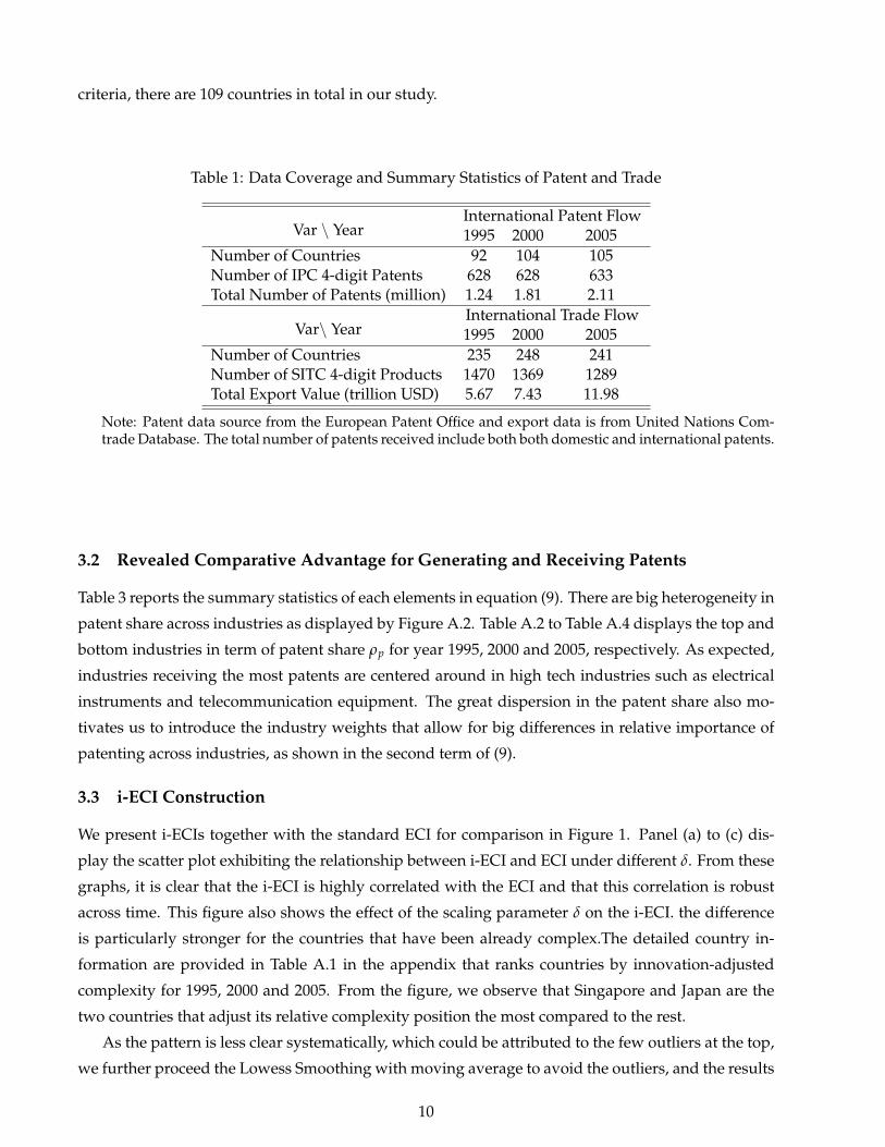
criteria, there are 109 countries in total in our study.
Table 1: Data Coverage and Summary Statistics of Patent and Trade
Var \ YearInternational Patent Flow1995 2000 2005
Number of Countries 92 104 105Number of IPC 4-digit Patents 628 628 633Total Number of Patents (million) 1.24 1.81 2.11
Var\ YearInternational Trade Flow1995 2000 2005
Number of Countries 235 248 241Number of SITC 4-digit Products 1470 1369 1289Total Export Value (trillion USD) 5.67 7.43 11.98
Note: Patent data source from the European Patent Office and export data is from United Nations Com-trade Database. The total number of patents received include both both domestic and international patents.
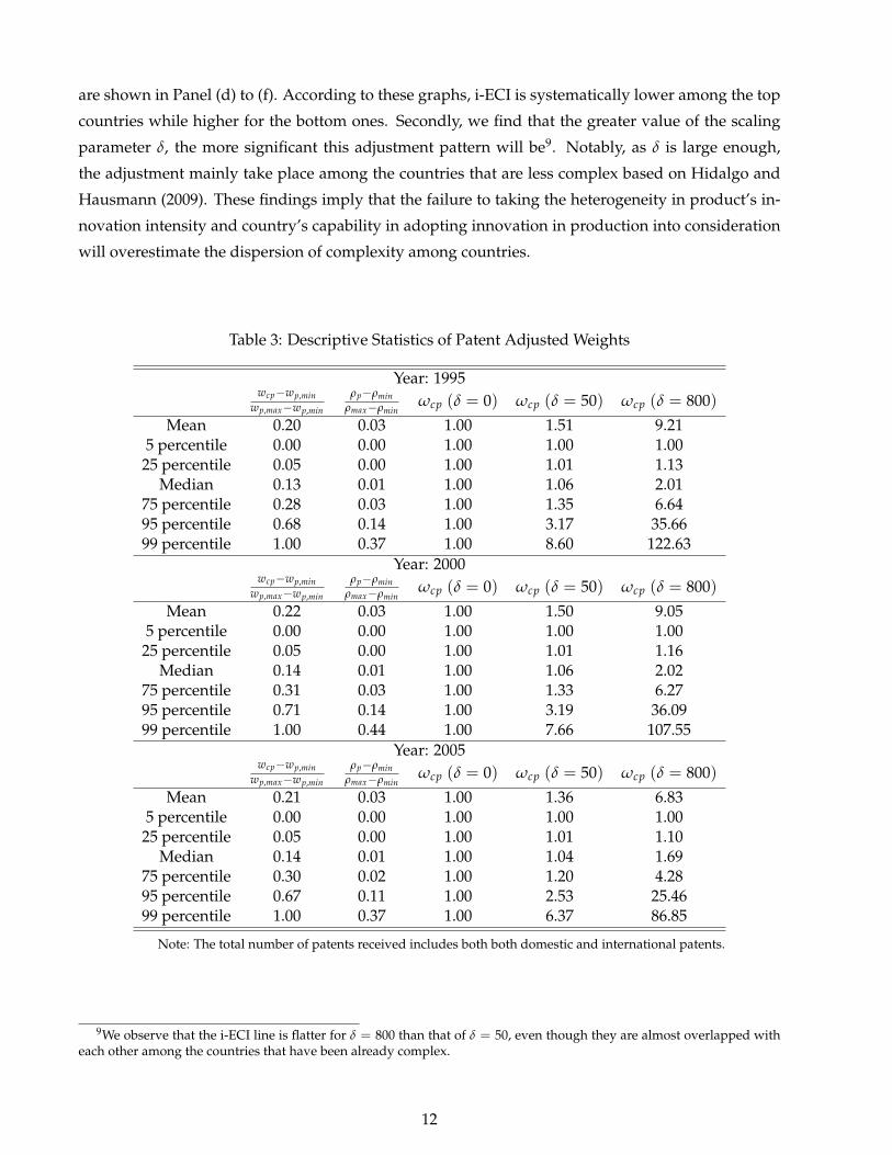
3.2 Revealed Comparative Advantage for Generating and Receiving Patents
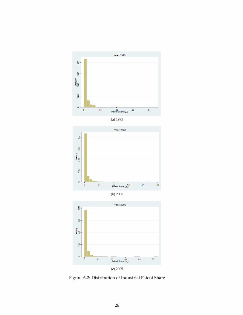
Table 3 reports the summary statistics of each elements in equation (9). There are big heterogeneity in
patent share across industries as displayed by Figure A.2. Table A.2 to Table A.4 displays the top and
bottom industries in term of patent share ρp for year 1995, 2000 and 2005, respectively. As expected,
industries receiving the most patents are centered around in high tech industries such as electrical
instruments and telecommunication equipment. The great dispersion in the patent share also mo-
tivates us to introduce the industry weights that allow for big differences in relative importance of
patenting across industries, as shown in the second term of (9).
3.3 i-ECI Construction
We present i-ECIs together with the standard ECI for comparison in Figure 1. Panel (a) to (c) dis-
play the scatter plot exhibiting the relationship between i-ECI and ECI under different δ. From these
graphs, it is clear that the i-ECI is highly correlated with the ECI and that this correlation is robust
across time. This figure also shows the effect of the scaling parameter δ on the i-ECI. the difference
is particularly stronger for the countries that have been already complex.The detailed country in-
formation are provided in Table A.1 in the appendix that ranks countries by innovation-adjusted
complexity for 1995, 2000 and 2005. From the figure, we observe that Singapore and Japan are the
two countries that adjust its relative complexity position the most compared to the rest.
As the pattern is less clear systematically, which could be attributed to the few outliers at the top,
we further proceed the Lowess Smoothing with moving average to avoid the outliers, and the results
10

Table 2: Top Exporters and Patent Receivers
Top 10 Patent ReceiversRank\Year 1995 2000 2005
1 Japan Japan United States2 United States United States Japan3 Germany Germany China4 China China Republic of Korea5 Republic of Korea Australia Germany6 Australia Republic of Korea Canada7 Spain Spain Russia8 United Kingdom Canada Brazil9 France France France10 Canada Austria Taiwan
Top 10 ExportersRank\Year 1995 2000 2005
1 United States United States China2 Germany Germany Germany3 Japan Japan United States4 France China Japan5 United Kingdom France France6 China United Kingdom United Kingdom7 Italy Canada Netherlands8 Canada Italy Italy9 Netherlands Netherlands Canada10 Hong Kong Hong Kong Belgium
Note: The total number of patents received includes both both domestic and international patents.
11
are shown in Panel (d) to (f). According to these graphs, i-ECI is systematically lower among the top
countries while higher for the bottom ones. Secondly, we find that the greater value of the scaling
parameter δ, the more significant this adjustment pattern will be9. Notably, as δ is large enough,
the adjustment mainly take place among the countries that are less complex based on Hidalgo and
Hausmann (2009). These findings imply that the failure to taking the heterogeneity in product’s in-
novation intensity and country’s capability in adopting innovation in production into consideration
will overestimate the dispersion of complexity among countries.
Table 3: Descriptive Statistics of Patent Adjusted Weights
Year: 1995wcp−wp,min
wp,max−wp,min
ρp−ρminρmax−ρmin
ωcp (δ = 0) ωcp (δ = 50) ωcp (δ = 800)
Mean 0.20 0.03 1.00 1.51 9.215 percentile 0.00 0.00 1.00 1.00 1.00
25 percentile 0.05 0.00 1.00 1.01 1.13Median 0.13 0.01 1.00 1.06 2.01
75 percentile 0.28 0.03 1.00 1.35 6.6495 percentile 0.68 0.14 1.00 3.17 35.6699 percentile 1.00 0.37 1.00 8.60 122.63
Year: 2000wcp−wp,min
wp,max−wp,min
ρp−ρminρmax−ρmin
ωcp (δ = 0) ωcp (δ = 50) ωcp (δ = 800)
Mean 0.22 0.03 1.00 1.50 9.055 percentile 0.00 0.00 1.00 1.00 1.00
25 percentile 0.05 0.00 1.00 1.01 1.16Median 0.14 0.01 1.00 1.06 2.02
75 percentile 0.31 0.03 1.00 1.33 6.2795 percentile 0.71 0.14 1.00 3.19 36.0999 percentile 1.00 0.44 1.00 7.66 107.55
Year: 2005wcp−wp,min
wp,max−wp,min
ρp−ρminρmax−ρmin
ωcp (δ = 0) ωcp (δ = 50) ωcp (δ = 800)
Mean 0.21 0.03 1.00 1.36 6.835 percentile 0.00 0.00 1.00 1.00 1.00
25 percentile 0.05 0.00 1.00 1.01 1.10Median 0.14 0.01 1.00 1.04 1.69
75 percentile 0.30 0.02 1.00 1.20 4.2895 percentile 0.67 0.11 1.00 2.53 25.4699 percentile 1.00 0.37 1.00 6.37 86.85
Note: The total number of patents received includes both both domestic and international patents.
9We observe that the i-ECI line is flatter for δ = 800 than that of δ = 50, even though they are almost overlapped witheach other among the countries that have been already complex.
12

(a)1
995
(b)2
000
(c)2
005
(d)1
995
(e)2
000
(f)2
005
Not
e:Fi
gure
(d)t
oFi
gure
(f)e
xhib
itth
eLo
wes
sSm
ooth
ing
fitte
dlin
esfo
rFi
gure
(a)t
oFi
gure
(c),
whi
char
eob
tain
edfr
omru
nnin
g-m
ean
smoo
th.
Figu
re1:
ECIa
ndIn
nova
tion
-adj
uste
dEC
ICom
pari
son
13

4 Analysis and Results
In this section, we examine to what extent that the innovation-adjusted complexity index promote
the long run economic growth (from 1995 to 2005). We adopt one simple version of specification used
in Hidalgo and Hausmann (2009):
ln(GDPi(t + ∆t)
GDPi(t)) = a + b1 GDPi(t) + b2iECIi(t) + eit (11)
where GDPi(t) is per capita GDP for country i in year t, and iECIi(t) is the Innovation-adjusted Eco-
nomic Complexity Index of country i in year t (note thatiECIi(t) is identical ECIi(t) when δ is zero).
We use the five-year growth rate of per capita GDP as the dependent variable. In the regression,
we also control for the income level of the initial level, and the sample are from 1995 to 2005. Our
interests associated with the regression is to study whether the introduction of innovation will bring
an extra improvement in predicting the long run economic growth, as well as to study the role of
i-ECI in generating the economic growth.
Table 4: Effect of Innovation-adjusted Complexity Index on the Long Run Economic Growth
Dept Var: Growth of PGDP ECI = iECI i-ECI(δ = 50) i-ECI(δ = 800)
i-ECI 0.0533* 0.0641** 0.0740**(0.0291) (0.0293) (0.0298)
PGDP -0.162*** -0.168*** -0.174***(0.0233) (0.0234) (0.0238)
Constant 0.753*** 0.758*** 0.764***(0.0298) (0.0298) (0.0300)
Observations 324 324 324R-squared 0.166 0.170 0.173
Note: standard errors are reported in parentheses; *** p<0.01, ** p<0.05, * p<0.1.
Table 4 presents the regression results. The first column is our reference specification that corre-
sponds to the case where δ = 0 (the same with ECI in Hidalgo and Hausmann (2009)). The second
and third columns exhibit the results when δ equals 50 and 800, respectively. The coefficients of all
the specifications are consistent with Hidalgo and Hausmann (2009), i.e., the growth rate of aver-
age income is faster when a country has lower level in initial average income and is more complex.
Comparing the second and third columns to our reference specification, we find that the innovation-
adjusted complexity index has a stronger effect on income growth than the complexity measure with-
out taking care of the patent flow, and such impact increases with the patent intensity parameter δ.
14
In the mean while, we also find that models incorporating patent flow explain a larger proportion
than the reference specification. This sheds lights on the important role of patent flow in promoting
the worldwide economic development.
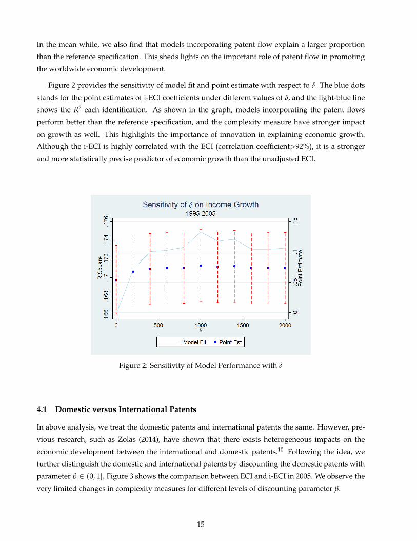
Figure 2 provides the sensitivity of model fit and point estimate with respect to δ. The blue dots
stands for the point estimates of i-ECI coefficients under different values of δ, and the light-blue line
shows the R2 each identification. As shown in the graph, models incorporating the patent flows
perform better than the reference specification, and the complexity measure have stronger impact
on growth as well. This highlights the importance of innovation in explaining economic growth.
Although the i-ECI is highly correlated with the ECI (correlation coefficient>92%), it is a stronger
and more statistically precise predictor of economic growth than the unadjusted ECI.
Figure 2: Sensitivity of Model Performance with δ
4.1 Domestic versus International Patents
In above analysis, we treat the domestic patents and international patents the same. However, pre-
vious research, such as Zolas (2014), have shown that there exists heterogeneous impacts on the
economic development between the international and domestic patents.10 Following the idea, we
further distinguish the domestic and international patents by discounting the domestic patents with
parameter β ∈ (0, 1]. Figure 3 shows the comparison between ECI and i-ECI in 2005. We observe the
very limited changes in complexity measures for different levels of discounting parameter β.
15

(a)
β=
0.25
(b)
β=
0.5
(c)
β=
0.75
Figu
re3:
ECIa
ndIn
nova
tion
-adj
uste
dEC
ICom
pari
son
acro
ssβ
(200
5)
(a)Y
ear:
1995
(b)Y
ear:
2000
(c)Y
ear:
2005
Figu
re4:
Dis
coun
tRat
eon
Dom
esti
cPa
tent
san
dC
hang
eof
i-EC
I
16

To study how domestic patents influence on a country’s i-ECI, we further display the relationship
between the change of a country’s i-ECI and his domestic patent share, as is shown in Figure 4. The
vertical axis display the i-ECI changes when discounting the domestic patents from rate β = 0.75 to
β = 0. We observe the positive correlation between i-ECI changes and a country’s domestic patent
share, which indicates that domestic patents improves a country’s complexity level (and this pattern
across all the sample years). Figure A.3 in the Appendix provides the change of i-ECI rank for the
top thirty countries. Table A.5 reports the regression results of (11) with different discounting rates.
We do not find any systematic difference in the impacts of innovation on the economic growth via
climbing up the complexity ladder between the domestic and international patents.
5 Conclusion
In the paper, we propose an Innovation-adjusted ECI (i-ECI) that uses a high-resolution patent-trade
concordance to construct trade networks weighted by domestic and international patent application
flows. The i-ECI thereby reflects firms’ decisions about where to seek patent protection on industry-
specific inventions, allows for heterogeneity in the relative importance of patenting across industries,
and implicitly captures firms’ perceived innovation potential in the recipient countries. Our empiri-
cal exercise reveals that incorporating the patent flows could explain more on the economic growth
in terms of GDP per-capita compared to the unadjusted ECI measure as developed byHidalgo and
Hausmann (2009). In addition, we find that the complexity measure has a stronger impact on growth
after taking care of patent flows. This highlights the importance of innovation in explaining economic
growth. Although the i-ECI is highly correlated with the ECI (correlation coefficient>92%), we be-
lieve it is a stronger and more statistically precise predictor of economic growth than the unadjusted
ECI.
10For instance, Zolas (2014) finds that international patents are associated with more sophisticated technology. In thefollowing part, we explore such heterogeneous implications by international and domestic patents.
17

References
ACS, Z. J., L. ANSELIN, AND A. VARGA (2002): “Patents and innovation counts as measures of
regional production of new knowledge,” Research policy, 31(7), 1069–1085.
AZAM, S. (2017): “A cross-country empirical test of cognitive abilities and innovation nexus,” Inter-
national Journal of Educational Development, 53, 128–136.
CHILICHES, Z. (1990): “Indicators: A Survey,” Journal ofEconomic Literature, 28(4), 1661–1707.
DONOSO, J. F. (2017): “A simple index of innovation with complexity,” Journal of Informetrics, 11(1),
1–17.
GRILICHES, Z. (1998): “Patent statistics as economic indicators: a survey,” in R&D and productivity:
the econometric evidence, pp. 287–343. University of Chicago Press.
HAUSMANN, R., AND C. A. HIDALGO (2011): “The network structure of economic output,” Journal
of Economic Growth, 16(4), 309–342.
HEKKERT, M. P., R. A. SUURS, S. O. NEGRO, S. KUHLMANN, AND R. E. SMITS (2007): “Functions of
innovation systems: A new approach for analysing technological change,” Technological forecasting
and social change, 74(4), 413–432.
HIDALGO, C. A., AND R. HAUSMANN (2009): “The building blocks of economic complexity,” pro-
ceedings of the national academy of sciences, 106(26), 10570–10575.
IVANOVA, I., Ø. STRAND, D. KUSHNIR, AND L. LEYDESDORFF (2017): “Economic and technological
complexity: A model study of indicators of knowledge-based innovation systems,” Technological
Forecasting and Social Change.
LYBBERT, T. J., AND N. J. ZOLAS (2014): “Getting patents and economic data to speak to each other:
An ‘algorithmic links with probabilities’ approach for joint analyses of patenting and economic
activity,” Research Policy, 43(3), 530–542.
NELSON, R. R., AND K. NELSON (2002): “Technology, institutions, and innovation systems,” Research
policy, 31(2), 265–272.
SWEET, C. M., AND D. S. E. MAGGIO (2015): “Do stronger intellectual property rights increase inno-
vation?,” World Development, 66, 665–677.
ZOLAS, N. (2014): “International Patenting Strategies with Heterogeneous Firms,” Discussion paper,
US Census Bureau, Center for Economic Studies.
18
Appendix
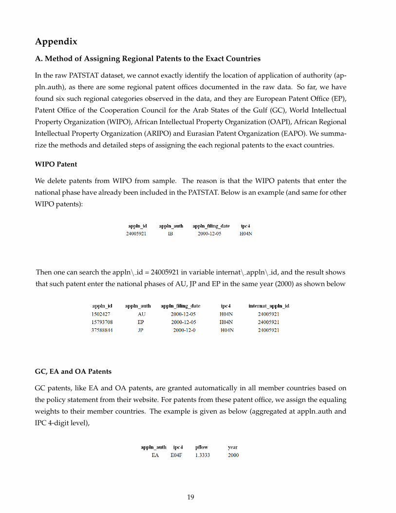
A. Method of Assigning Regional Patents to the Exact Countries
In the raw PATSTAT dataset, we cannot exactly identify the location of application of authority (ap-
pln auth), as there are some regional patent offices documented in the raw data. So far, we have
found six such regional categories observed in the data, and they are European Patent Office (EP),
Patent Office of the Cooperation Council for the Arab States of the Gulf (GC), World Intellectual
Property Organization (WIPO), African Intellectual Property Organization (OAPI), African Regional
Intellectual Property Organization (ARIPO) and Eurasian Patent Organization (EAPO). We summa-
rize the methods and detailed steps of assigning the each regional patents to the exact countries.
WIPO Patent
We delete patents from WIPO from sample. The reason is that the WIPO patents that enter the
national phase have already been included in the PATSTAT. Below is an example (and same for other
WIPO patents):
Then one can search the appln\ id = 24005921 in variable internat\ appln\ id, and the result shows
that such patent enter the national phases of AU, JP and EP in the same year (2000) as shown below
GC, EA and OA Patents
GC patents, like EA and OA patents, are granted automatically in all member countries based on
the policy statement from their website. For patents from these patent office, we assign the equaling
weights to their member countries. The example is given as below (aggregated at appln auth and
IPC 4-digit level),
19
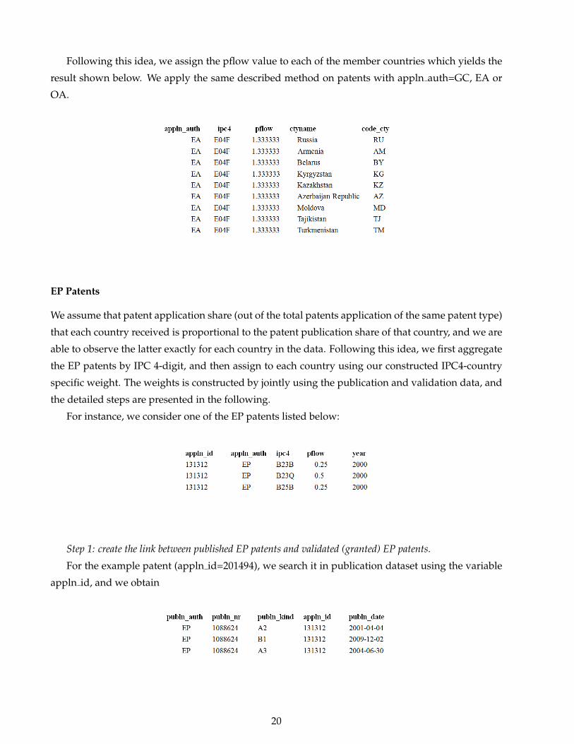
Following this idea, we assign the pflow value to each of the member countries which yields the
result shown below. We apply the same described method on patents with appln auth=GC, EA or
OA.
EP Patents
We assume that patent application share (out of the total patents application of the same patent type)
that each country received is proportional to the patent publication share of that country, and we are
able to observe the latter exactly for each country in the data. Following this idea, we first aggregate
the EP patents by IPC 4-digit, and then assign to each country using our constructed IPC4-country
specific weight. The weights is constructed by jointly using the publication and validation data, and
the detailed steps are presented in the following.
For instance, we consider one of the EP patents listed below:
Step 1: create the link between published EP patents and validated (granted) EP patents.
For the example patent (appln id=201494), we search it in publication dataset using the variable
appln id, and we obtain
20
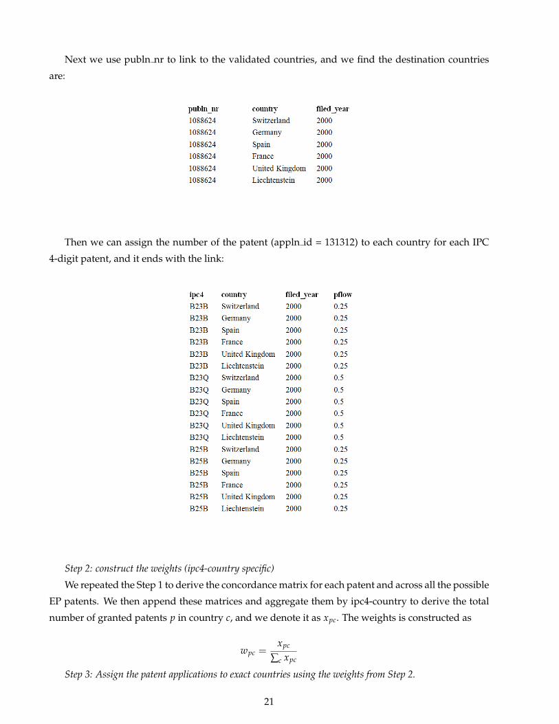
Next we use publn nr to link to the validated countries, and we find the destination countries
are:
Then we can assign the number of the patent (appln id = 131312) to each country for each IPC
4-digit patent, and it ends with the link:
Step 2: construct the weights (ipc4-country specific)
We repeated the Step 1 to derive the concordance matrix for each patent and across all the possible
EP patents. We then append these matrices and aggregate them by ipc4-country to derive the total
number of granted patents p in country c, and we denote it as xpc. The weights is constructed as
wpc =xpc
∑c xpc
Step 3: Assign the patent applications to exact countries using the weights from Step 2.
21

Given the aggregated patents at ipc4 level Xp, we assign them to each countries using wpc for any
c and p:
Xpc = Xp × wpc
AP Patents
For these patents, we are not able to distinguish between the member countries, as they adopt the
policy of ex-ante designation, i.e., a granted patent only has effect in the countries that were desig-
nated at the application stage. However, as the total number of patents from AP is small in quantity,
it will not make a great difference in our analysis.
22

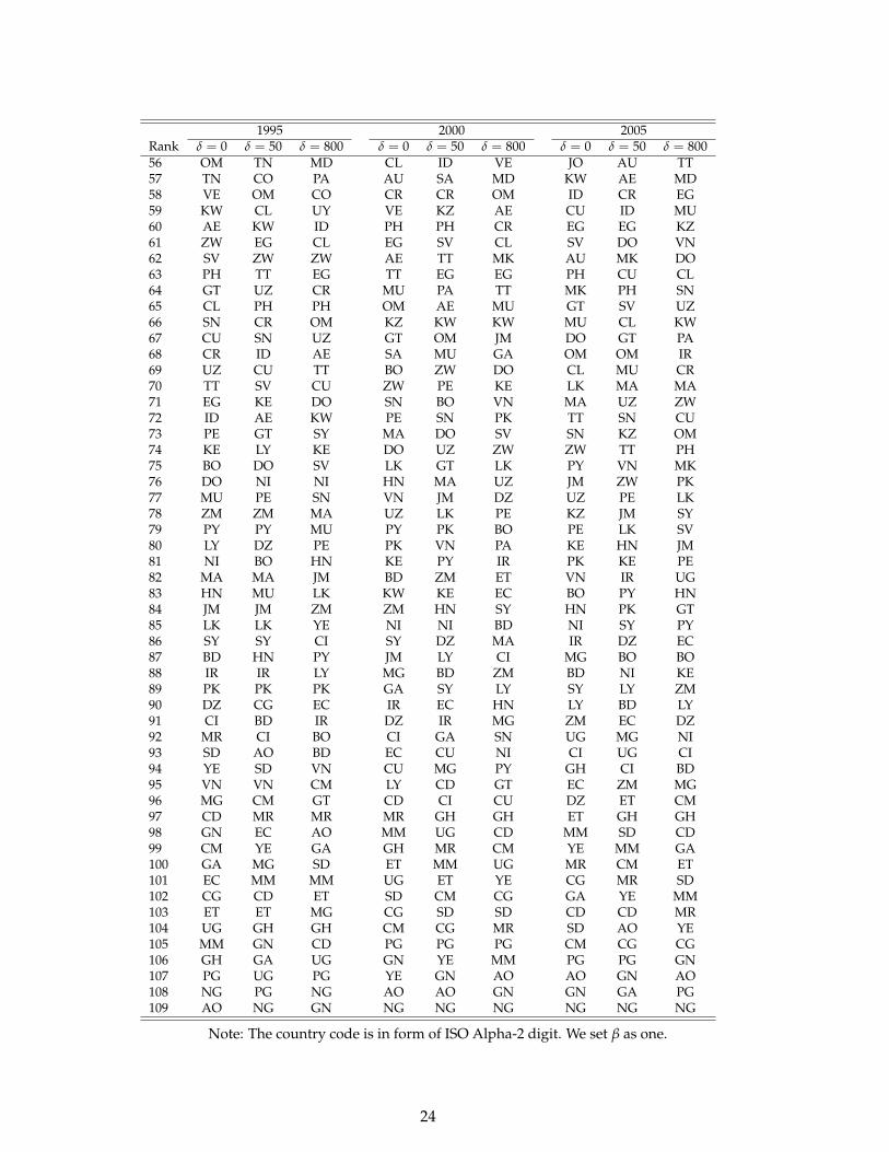
Table A.1: Country Complexity Ranks
1995 2000 2005Rank δ = 0 δ = 50 δ = 800 δ = 0 δ = 50 δ = 800 δ = 0 δ = 50 δ = 8001 JP JP JP JP JP SG JP JP JP2 DE SE SE DE DE JP DE DE SG3 CH DE DE CH CH SE CH SE DE4 SE CH SG SE SE CH AT CH FI5 AT FI CH GB GB DE SE FI SE6 FI AT FI AT FI FI FI AT CH7 GB GB GB US AT GB GB GB AT8 US FR AT FI US US CZ CZ GB9 FR US FR FR FR AT FR SG CZ10 IT IT IT IT IT IT SI KR KR11 DK CZ US CZ CZ FR US US SI12 SI SI CZ DK SG CZ SG SI US13 CZ DK SI SI SI IE KR FR FR14 SK ES KR IE DK KR IE IT SK15 NL SK DK IL IE IL IT HU HU16 IE SG CA KR IL DK DK IE IT17 ES NL ES SK KR SI HU DK IE18 IL IL NO NL NL MX SK SK CA19 SG IE NL SG SK NL NL NL DK20 KR CA IL ES ES ES MX BY NL21 CA NO IE MX MX CA BY ES NO22 HU KR SK HU CA PL IL IL PL23 PL BR BR PL HU HU ES NO BY24 MX MX MX BY PL SK PL MX ES25 NO HU PL CA BY NO HR PL IL26 HR PL HU HK RU RU HK CA RO27 EE HR HK HR BR BR CA HR BR28 BR RO HR BR NO HK NO EE UA29 BY EE RO RU RO BY PT LT MX30 RO KZ RU PT PT PT EE LV RU31 HK BY EE UA HK RO MY RO LT32 PT PT AU LV UA UA LV UA LV33 LT BG NZ RO HR CN LT BR EE34 KZ NZ BY NO LV LV RO RU BG35 BG RU PT EE EE NZ CN HK HK36 LV HK BG BG BG EE UA PT HR37 RU LT AR MY LT HR RU BG PT38 MK LV LT LT JO MY BR MY TR39 MD AU LV TH CN LT TH CN CN40 NZ UA KZ JO NZ ZA BG NZ NZ41 UA ZA ZA CN AR BG NZ TH AR42 ZA AR IN NZ TH TH SA SA GR43 UY MK CN IN MY AR TR TR MY44 MY SA MY GR IN TR IN AR TH45 AR MY UA TR TR JO AR IN ZA46 CN JO CG UY GR SA GR GR AU47 TH CN TH MD ZA AU UY ZA JO48 JO MD GR ZA UY PH PA UY TN49 AU TR JO AR CO GR CO TN AE50 SA GR VE CO MD TN ZA CO SA51 TR TH TR PA MK IN MD JO ID52 GR UY MK TN TN CO TN PA VE53 PA VE SA SV AU ID AE MD IN54 IN IN DZ ID CL UY CR VE CO55 CO PA TN MK VE KZ VE KW UY
23
1995 2000 2005Rank δ = 0 δ = 50 δ = 800 δ = 0 δ = 50 δ = 800 δ = 0 δ = 50 δ = 80056 OM TN MD CL ID VE JO AU TT57 TN CO PA AU SA MD KW AE MD58 VE OM CO CR CR OM ID CR EG59 KW CL UY VE KZ AE CU ID MU60 AE KW ID PH PH CR EG EG KZ61 ZW EG CL EG SV CL SV DO VN62 SV ZW ZW AE TT MK AU MK DO63 PH TT EG TT EG EG PH CU CL64 GT UZ CR MU PA TT MK PH SN65 CL PH PH OM AE MU GT SV UZ66 SN CR OM KZ KW KW MU CL KW67 CU SN UZ GT OM JM DO GT PA68 CR ID AE SA MU GA OM OM IR69 UZ CU TT BO ZW DO CL MU CR70 TT SV CU ZW PE KE LK MA MA71 EG KE DO SN BO VN MA UZ ZW72 ID AE KW PE SN PK TT SN CU73 PE GT SY MA DO SV SN KZ OM74 KE LY KE DO UZ ZW ZW TT PH75 BO DO SV LK GT LK PY VN MK76 DO NI NI HN MA UZ JM ZW PK77 MU PE SN VN JM DZ UZ PE LK78 ZM ZM MA UZ LK PE KZ JM SY79 PY PY MU PY PK BO PE LK SV80 LY DZ PE PK VN PA KE HN JM81 NI BO HN KE PY IR PK KE PE82 MA MA JM BD ZM ET VN IR UG83 HN MU LK KW KE EC BO PY HN84 JM JM ZM ZM HN SY HN PK GT85 LK LK YE NI NI BD NI SY PY86 SY SY CI SY DZ MA IR DZ EC87 BD HN PY JM LY CI MG BO BO88 IR IR LY MG BD ZM BD NI KE89 PK PK PK GA SY LY SY LY ZM90 DZ CG EC IR EC HN LY BD LY91 CI BD IR DZ IR MG ZM EC DZ92 MR CI BO CI GA SN UG MG NI93 SD AO BD EC CU NI CI UG CI94 YE SD VN CU MG PY GH CI BD95 VN VN CM LY CD GT EC ZM MG96 MG CM GT CD CI CU DZ ET CM97 CD MR MR MR GH GH ET GH GH98 GN EC AO MM UG CD MM SD CD99 CM YE GA GH MR CM YE MM GA100 GA MG SD ET MM UG MR CM ET101 EC MM MM UG ET YE CG MR SD102 CG CD ET SD CM CG GA YE MM103 ET ET MG CG SD SD CD CD MR104 UG GH GH CM CG MR SD AO YE105 MM GN CD PG PG PG CM CG CG106 GH GA UG GN YE MM PG PG GN107 PG UG PG YE GN AO AO GN AO108 NG PG NG AO AO GN GN GA PG109 AO NG GN NG NG NG NG NG NG
Note: The country code is in form of ISO Alpha-2 digit. We set β as one.
24

B. Appendix for Tables and Figures
(a) 1995
(b) 2000
(c) 2005
Figure A.1: The ECI and i-ECI Rank (Top 30 Countries by ECI)25
(a) 1995
(b) 2000
(c) 2005
Figure A.2: Distribution of Industrial Patent Share
26
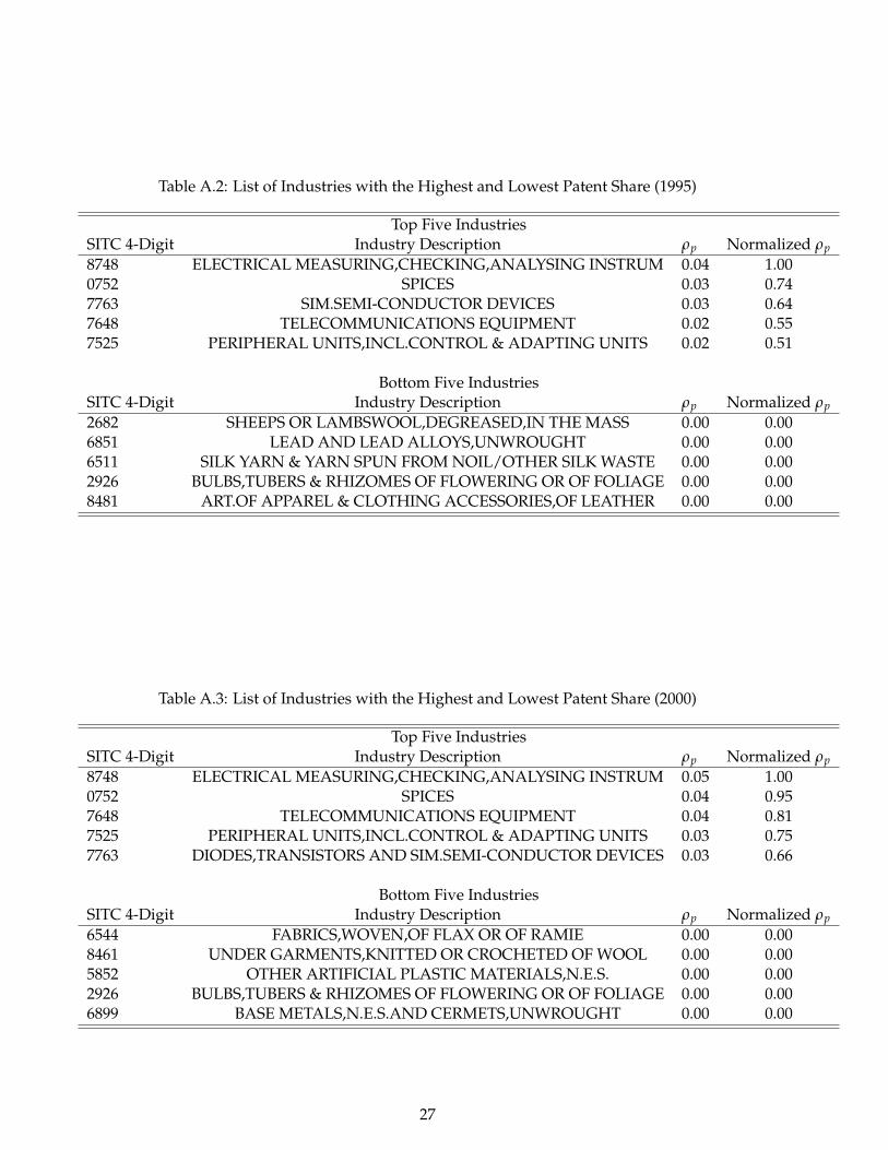
Table A.2: List of Industries with the Highest and Lowest Patent Share (1995)
Top Five IndustriesSITC 4-Digit Industry Description ρp Normalized ρp8748 ELECTRICAL MEASURING,CHECKING,ANALYSING INSTRUM 0.04 1.000752 SPICES 0.03 0.747763 SIM.SEMI-CONDUCTOR DEVICES 0.03 0.647648 TELECOMMUNICATIONS EQUIPMENT 0.02 0.557525 PERIPHERAL UNITS,INCL.CONTROL & ADAPTING UNITS 0.02 0.51
Bottom Five IndustriesSITC 4-Digit Industry Description ρp Normalized ρp2682 SHEEPS OR LAMBSWOOL,DEGREASED,IN THE MASS 0.00 0.006851 LEAD AND LEAD ALLOYS,UNWROUGHT 0.00 0.006511 SILK YARN & YARN SPUN FROM NOIL/OTHER SILK WASTE 0.00 0.002926 BULBS,TUBERS & RHIZOMES OF FLOWERING OR OF FOLIAGE 0.00 0.008481 ART.OF APPAREL & CLOTHING ACCESSORIES,OF LEATHER 0.00 0.00
Table A.3: List of Industries with the Highest and Lowest Patent Share (2000)
Top Five IndustriesSITC 4-Digit Industry Description ρp Normalized ρp8748 ELECTRICAL MEASURING,CHECKING,ANALYSING INSTRUM 0.05 1.000752 SPICES 0.04 0.957648 TELECOMMUNICATIONS EQUIPMENT 0.04 0.817525 PERIPHERAL UNITS,INCL.CONTROL & ADAPTING UNITS 0.03 0.757763 DIODES,TRANSISTORS AND SIM.SEMI-CONDUCTOR DEVICES 0.03 0.66
Bottom Five IndustriesSITC 4-Digit Industry Description ρp Normalized ρp6544 FABRICS,WOVEN,OF FLAX OR OF RAMIE 0.00 0.008461 UNDER GARMENTS,KNITTED OR CROCHETED OF WOOL 0.00 0.005852 OTHER ARTIFICIAL PLASTIC MATERIALS,N.E.S. 0.00 0.002926 BULBS,TUBERS & RHIZOMES OF FLOWERING OR OF FOLIAGE 0.00 0.006899 BASE METALS,N.E.S.AND CERMETS,UNWROUGHT 0.00 0.00
27
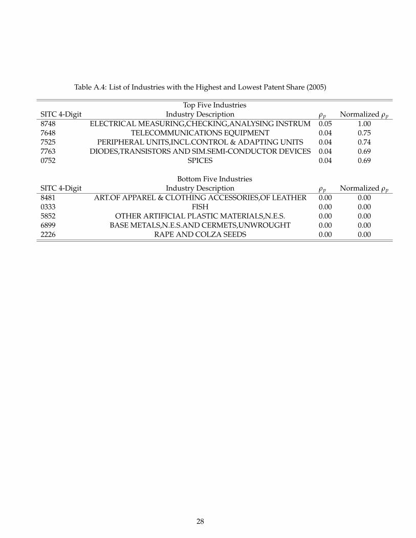
Table A.4: List of Industries with the Highest and Lowest Patent Share (2005)
Top Five IndustriesSITC 4-Digit Industry Description ρp Normalized ρp8748 ELECTRICAL MEASURING,CHECKING,ANALYSING INSTRUM 0.05 1.007648 TELECOMMUNICATIONS EQUIPMENT 0.04 0.757525 PERIPHERAL UNITS,INCL.CONTROL & ADAPTING UNITS 0.04 0.747763 DIODES,TRANSISTORS AND SIM.SEMI-CONDUCTOR DEVICES 0.04 0.690752 SPICES 0.04 0.69
Bottom Five IndustriesSITC 4-Digit Industry Description ρp Normalized ρp8481 ART.OF APPAREL & CLOTHING ACCESSORIES,OF LEATHER 0.00 0.000333 FISH 0.00 0.005852 OTHER ARTIFICIAL PLASTIC MATERIALS,N.E.S. 0.00 0.006899 BASE METALS,N.E.S.AND CERMETS,UNWROUGHT 0.00 0.002226 RAPE AND COLZA SEEDS 0.00 0.00
28

Tabl
eA
.5:D
omes
tic
vers
usIn
tern
atio
nalP
aten
ts
Dep
tVar
:β=
0.10
β=
0.25
β=
0.50
β=
0.75
Gro
wth
ofPG
DP
δ=
50δ=
800
δ=
50δ=
800
δ=
50δ=
800
δ=
50δ=
800
i−E
CI
0.06
53**
0.07
39**
0.06
53**
0.07
47**
0.06
47**
0.07
06**
0.06
50**
0.07
36**
(0.0
291)
(0.0
293)
(0.0
294)
(0.0
298)
(0.0
293)
(0.0
298)
(0.0
293)
(0.0
298)
PG
DP
-0.1
69**
*-0
.174
***
-0.1
69**
*-0
.175
***
-0.1
68**
*-0
.172
***
-0.1
68**
*-0
.174
***
(0.0
234)
(0.0
240)
(0.0
235)
(0.0
238)
(0.0
234)
(0.0
238)
(0.0
234)
(0.0
238)
Con
stan
t0.
759*
**0.
764*
**0.
759*
**0.
764*
**0.
759*
**0.
762*
**0.
759*
**0.
764*
**(0
.029
8)(0
.030
1)(0
.029
8)(0
.030
0)(0
.029
8)(0
.030
0)(0
.029
8)(0
.030
0)
Obs
erva
tion
s32
432
432
432
432
432
432
432
4R
-squ
ared
0.17
00.
173
0.17
00.
174
0.17
00.
172
0.17
00.
173
Not
e:st
anda
rder
rors
are
repo
rted
inpa
rent
hese
s;**
*p<
0.01
,**
p<
0.05
,*p<
0.1.
29

(a) 1995
(b) 2000
(c) 2005
Figure A.3: i-ECI Rank and Discounting Rate of Domestic Patents (Top 30 Countries)
30