Innovation and Strategic Network Formation

Krishna Dasaratha∗

December 23, 2020Latest version available here

Abstract

We study a model of innovation with a large number of firms that create new technolo-

gies by combining several discrete ideas. These ideas are created via private investment

and spread between firms. Firms face a choice between secrecy, which protects existing

intellectual property, and openness, which facilitates learning from others. Their decisions

determine interaction rates between firms, and these interaction rates enter our model as

link probabilities in a learning network. Higher interaction rates impose both positive and

negative externalities, as there is more learning but also more competition. We show that

the equilibrium learning network is at a critical threshold between sparse and dense net-

works. At equilibrium, the positive externality from interaction dominates: the innovation

rate and welfare would be dramatically higher if the network were denser. So there are large

returns to increasing interaction rates above the critical threshold. Nevertheless, several nat-

ural types of interventions fail to move the equilibrium away from criticality. One effective

policy solution is to introduce informational intermediaries, such as public innovators who

do not have incentives to be secretive. These intermediaries can facilitate a high-innovation

equilibrium by transmitting ideas from one private firm to another.

∗University of Pennsylvania and Harvard University. Email: krishnadasaratha@gmail.com. I am deeply

grateful to Drew Fudenberg, Benjamin Golub, Matthew Rabin, and Tomasz Strzalecki for their guidance

and support. I would also like to thank Daron Acemoglu, Mohammad Akbarpour, Leonie Baumann, Yochai

Benkler, Laura Doval, Edward Glaeser, Kevin He, Nir Hak, Scott Kominers, Shengwu Li, Jonathan Libgober,

George Mailath, Michael Rose, Stefanie Stantcheva, Eduard Talamas, Omer Tamuz, Rakesh Vohra, and

Alexander Wolitzky for valuable comments and discussion.

1 Introduction

A growing body of empirical research suggests that interactions between inventors are an

important part of innovation.1 New technologies are often produced by combining individual

insights with learning from peers, which confers large benefits on firms and inventors engaged

in such learning.2 When highly-connected clusters of firms emerge in a location, as in the

technology industry in Silicon Valley, inventors in these areas are much more productive.

But frequent collaboration and learning are not assured even when inventors in a given

industry co-locate (Saxenian, 1996 gives a well-known example). Rather, interaction patterns

depend on firms’ decisions, such as how much to encourage their employees to interact

with employees from other firms. These interactions let a firm learn from other companies

and inventors. There are also downsides for the firm, as employees may share valuable

information. A more secretive approach allows firms to prevent potential competition by

protecting intellectual property. In making these types of decisions, firms and inventors

must choose between openness and secrecy.

We develop a theory of firms’ endogenous decisions about how much to interact with

other firms, and the consequences for information flows and the rate of innovation. Firms’

choices determine the probabilities of links in a learning network ; we thus contribute to

a theoretical literature on network formation.3 We show that at equilibrium, the learning

network has a special structure that would be unlikely to arise exogenously: it is at a critical

threshold between sparse and dense networks. This implies extreme inefficiencies arise at

equilibrium, and we analyze the welfare and policy implications.

We study a framework where each firm chooses two intensities: how open to be as well

as how much to invest in R&D. The choices of levels of openness determine interaction

rates between firms, and the probability that one firm learns from another is equal to the

interaction rate between the two firms. If a given firm is more open, that firm is more likely

to learn ideas from other firms—but other firms are more likely to learn its ideas. These

ideas are valuable because they can be combined to make new technologies, which are finite

1The benefits from interactions between inventors and movement of inventors have been quantified em-pirically by Akcigit, Caicedo, Miguelez, Stantcheva, and Sterzi (2018), Kerr (2008), Samila and Sorenson(2011), among others.

2See Bessen and Nuvolari (2016) for historical examples and Chesbrough (2003) for examples in thetechnology industry.

3An important feature of these choices is that firms combine different ideas to create new technologies(see also Acemoglu and Azar, 2019 and Chen and Elliott, 2019 for related combinatorial production func-tions). Strategic complementaries play a crucial role in many network games (e.g., Bramoulle, Kranton,and D’amours, 2014 and Ballester, Calvo-Armengol, and Zenou, 2006), and in our setting complementaritiesarise endogenously from this process of combining ideas.

1

sets of ideas (as in Weitzman, 1998). Firms can generate profits by producing technologies,

but the profits from a technology are erased by competition if another firm also knows the

component ideas in that technology.

Our first contribution, which is methodological, is to develop a theory of endogenous

formation of random networks in the context of our economic application. Learning oppor-

tunities are random events, and their realizations determine a learning network. We therefore

consider link formation decisions with uncertainty in the matching process, while the leading

approach in the literature on network-formation games focuses on deterministic models that

allow agents to choose particular links (Jackson and Wolinsky, 1996 and Bala and Goyal,

2000). Since we take actions to be continuous choices that translate to interaction rates,

optimal behavior satisfies first-order conditions rather than a high-dimensional system of

combinatorial inequalities.

A key feature of our model is that ideas can spread several steps through this network:

when one firm learns from another, the information transferred can include ideas learned

from a third firm. We refer to this as indirect learning.4 Under indirect learning, firms’

incentives depend on the global structure of the network. Each firm would like to learn

many ideas, since then the firm could combine these ideas to produce a large number of new

technologies, and much of this learning can be indirect.

Analyzing the global structure of the network leads to our second contribution, which is to

establish the criticality of equilibrium. When there are many firms, learning outcomes depend

dramatically on whether the learning network is sparsely connected or densely connected. If

firms’ interaction rates are below a critical threshold, the learning network consists of many

small clusters of firms who learn few ideas. Above the threshold, the learning network has

a giant component asymptotically: a large group of firms who learn a large number of ideas

and can incorporate these ideas into many new technologies (see Figure 1).5 To determine

where equilibrium lies with respect to this threshold, we analyze an individual firm’s decision

problem in each of these two domains, i.e. when other firms form a sparse or dense network.

The main result is that the equilibrium interaction rates are at the critical threshold

between sparse and dense networks. Firms would deviate to interact more if the network

were likely to be sparse, and deviate to interact less if the network were likely to be dense.

Intuitively, in sparse networks firms would increase interaction rates to fill central positions in

the network, known in sociology as ‘structural holes’, which enable the firm to combine ideas

4By contrast, existing work on strategic formation of random networks largely focuses on direct connec-tions (see, e.g., Currarini, Jackson, and Pin, 2009).

5Links are directed in the model, but undirected networks are shown in Figure 1 for illustrative purposes.

2

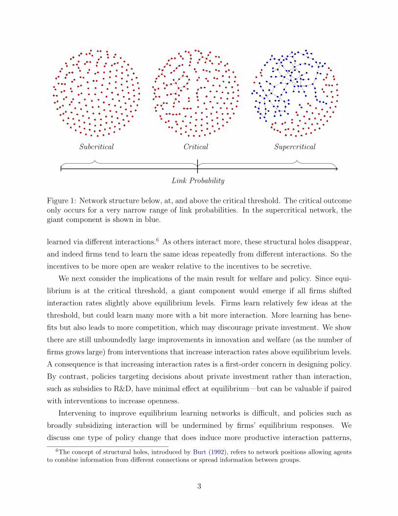
Subcritical Critical Supercritical

Link Probability

Figure 1: Network structure below, at, and above the critical threshold. The critical outcomeonly occurs for a very narrow range of link probabilities. In the supercritical network, thegiant component is shown in blue.

learned via different interactions.6 As others interact more, these structural holes disappear,

and indeed firms tend to learn the same ideas repeatedly from different interactions. So the

incentives to be more open are weaker relative to the incentives to be secretive.

We next consider the implications of the main result for welfare and policy. Since equi-

librium is at the critical threshold, a giant component would emerge if all firms shifted

interaction rates slightly above equilibrium levels. Firms learn relatively few ideas at the

threshold, but could learn many more with a bit more interaction. More learning has bene-

fits but also leads to more competition, which may discourage private investment. We show

there are still unboundedly large improvements in innovation and welfare (as the number of

firms grows large) from interventions that increase interaction rates above equilibrium levels.

A consequence is that increasing interaction rates is a first-order concern in designing policy.

By contrast, policies targeting decisions about private investment rather than interaction,

such as subsidies to R&D, have minimal effect at equilibrium—but can be valuable if paired

with interventions to increase openness.

Intervening to improve equilibrium learning networks is difficult, and policies such as

broadly subsidizing interaction will be undermined by firms’ equilibrium responses. We

discuss one type of policy change that does induce more productive interaction patterns,

6The concept of structural holes, introduced by Burt (1992), refers to network positions allowing agentsto combine information from different connections or spread information between groups.

3

which is to introduce public innovators who do not have incentives to be secretive. For

example, governments could fund academic researchers who are especially willing to interact

with other researchers, including those in industry. The key is that public innovators can

serve as informational intermediaries, transmitting ideas between private firms. They play a

valuable role even after considering the equilibrium response of the profit-maximizing firms,

who may adjust to be more secretive.

We next explore which features of the baseline model are needed to obtain a critical

equilibrium. One assumption is that learning probabilities are symmetric across pairs of

firms. We show that equilibrium remains critical even when firms have different propensities

to learn from others, which allows some firms to be better at protecting ideas than others.

The key feature driving the main result is that there is a margin along which firms can

acquire incoming links at the cost of a higher probability of outgoing links.

The criticality of equilibrium is robust to alternate specifications of the benefits from

learning from others but more sensitive to the costs of outgoing links. The baseline model

assumes firms’ profits are additive across technologies, but equilibrium remains critical if

there are increasing or slightly decreasing returns to producing many technologies. Indeed,

the crucial property is that payoffs are convex in the number of ideas learned by a firm.

Equilibrium outcomes do depend, however, on how much firms stand to lose from outgoing

links. In particular, the results described above assume zero profits in competitive markets.

If profits under competition are instead positive (e.g., because of a first-mover advantage or

markets with collusion between firms), then incentives toward secrecy will be weaker and so

equilibria will be above the critical threshold. These results give testable predictions about

the relationship between market structure and outcomes such as the innovation rate.

Our final results ask how formal intellectual property rights change the incentives to

interact. Consider the consequences of granting patents to a positive fraction of ideas, e.g.,

allowing hardware but not software ideas to be patented. Patents mitigate firms’ incentives

to be secretive, but can also discourage exchange of ideas. Firms with patents are more open

but are also less desirable partners in interactions (at least when ideas are only transmitted

directly). The resulting adverse selection in interaction can deter firms from collaborating

with others. We show that patent rights can therefore prevent any productive interactions

at equilibrium. If indirect learning is important, firms with patents will be informational

intermediaries, like the public innovators above. In this case there are benefits to allowing

patents, but it turns out that the optimal policy is often to only allow patents for a very

small fraction of ideas.

4

At a technical level, this paper develops tools for studying incentives in random network

settings. These tools are most applicable to analyzing decisions in network models with

complementarities between indirect connections. Classical results in graph theory character-

ize the component structure of large random networks, and thus in our context the number

of ideas firms will learn (Karp, 1990 and Luczak, 1990). But due to the complementari-

ties between ideas, firms’ incentives also depend on how these ideas are learned, e.g., via

many interactions or a few interactions. To capture these complementarities, we prove a key

lemma relating a firm’s equilibrium action to the extent to which technologies combine ideas

from distinct interactions. An additional challenge is that to understand incentives, it is not

enough to analyze “leading terms”. Vanishing-probability events and lower-order terms in

link probabilities could substantially affect payoffs. Our analysis therefore requires careful

treatment of the graph branching process governing the number of ideas learned from each

interaction.

1.1 Related Literature

This paper relates to research in network theory, especially network formation, and to models

of innovation.

At a methodological level, we develop a theory of strategic network formation with prob-

abilistic links. A large literature since Jackson and Wolinsky (1996) and Bala and Goyal

(2000) considers endogenous network formation assuming that agents can choose their links

exactly.7 Because equilibrium is then characterized by a large system of inequalities, these

models illustrate key externalities in special cases but remain largely or entirely intractable

in many others. By instead considering agents making a single choice about openness un-

der uncertainty, we obtain a smooth model of link formation that can be solved via basic

optimization techniques combined with analyses of random graphs.

Under this random-network model of network formation, incentives to form links depend

on the ‘phase transitions’ between sparse and dense networks.8 Economic models involving

phase transitions have been recently explored in the context of diffusion processes by Camp-

bell (2013), Akbarpour, Malladi, and Saberi (2018), and Sadler (2020). These models let

adoption and/or seeding decisions depend on component structure in an underlying network.

7The pairwise stability solution concept from Jackson and Wolinsky (1996) and variants have been appliedto network formation in many settings, including innovation (Konig, Battiston, Napoletano, and Schweitzer,2011, Konig, Battiston, Napoletano, and Schweitzer, 2012).

8Golub and Livne (2010) also study network formation with phase transitions, and allow payoffs to dependon distance one and two connections. An important feature of our model is that firms’ decisions depend onthe global network structure rather than only local connections.

5

We instead study equilibria of a game in which agents endogenously make decisions about

how much to interact with others, and find there is a subtle interplay between strategic

incentives and the global network structure.

An alternate approach to smooth network formation is to consider weighted networks, so

that each link has an intensity (as in Cabrales, Calvo-Armengol, and Zenou, 2011, Baumann,

2017, and Griffith, 2019). In some settings with unweighted links, this approach yields a

deterministic approximation of a game on the underlying random network. But for discrete

processes such as the diffusion of an idea, the random and deterministic models can be very

different. Indeed, we show that there is a critical threshold corresponding to important

discontinuities in network structure and outcomes that do not arise in deterministic models

such as Cabrales, Calvo-Armengol, and Zenou (2011).9

In existing literature on innovation, approaches incorporating interactions between firms

generally model these interactions as either mechanical spillovers or learning via imitation. A

common approach is to choose a convenient functional form for spillovers, usually motivated

by tractability within a macroeconomic (e.g., Kortum, 1997) or network-theory (Konig, Bat-

tiston, Napoletano, and Schweitzer, 2012) framework.10 By microfounding these spillovers,

which arise endogenously within the innovative process, we can study how spillovers respond

to policy interventions.

In a different approach, which relies on a quality-ladders framework, interactions give

firms a chance to catch up as innovation proceeds vertically through improvements in the

quality of existing technologies (e.g., Perla and Tonetti, 2014, Akcigit, Caicedo, Miguelez,

Stantcheva, and Sterzi, 2018, and Konig, Lorenz, and Zilibotti, 2016). We instead explicitly

model innovation horizontally as a process of combining distinct ideas, which serve as building

blocks for new technologies. Related models appear in Weitzman (1998) and Acemoglu and

Azar (2019), which focus on the evolution of the total amount of innovation over time and

do not involve learning or informational spillovers between firms. We find that when new

technologies can be created in this way, changes in interaction patterns can have much larger

consequences for the rate of innovation than in quality-ladders models.11

9Berliant and Fujita (2008) study a related deterministic model of knowledge creation with individualschoosing to producing knowledge alone or with a partner. Their analysis focuses on interaction patterns insmall disconnected groups, while we find social networks can be more connected in important ways.

10In simulations, Baum, Cowan, and Jonard (2010) study the formation of innovation networks via amechanical process.

11By assuming a continuum of firms, macroeconomic models of imitation often implicitly restrict to networkstructures without a giant component.

6

2 Model

We first describe our model formally and provide an example. We will then discuss inter-

pretations of the model and its assumptions.

2.1 Basic Setup

There are n > 1 firms 1, . . . , n. Each firm i can potentially discover a distinct idea, also

denoted by i. We let I ⊂ {1, . . . , n} be the set of ideas that are discovered.

Each firm i chooses a probability pi ∈ [0, 1) of discovering this idea and pays investment

cost c(pi). We will assume that c is continuously differentiable, increasing, and convex with

c(0) = 0 and limp→1− c(p) =∞. The realizations of discoveries are independent.

A technology t = {i1, . . . , ik} is a set of k ideas i1, . . . , ik ∈ I, where k > 1 is an

exogenous parameter capturing the complexity of technologies.12 The condition i1, . . . , ik ∈ Imeans that an idea i must be discovered by the corresponding firm to be included in a

technology.

Each firm i also chooses a level of openness qi ∈ [0, 1]. Given choices qi and qj, the

interaction rate between i and j is ι(qi, qj). We will assume the multiplicative interaction

rate

ι(qi, qj) = qiqj

except when a more general interaction rate is explicitly stated (in Theorem 1′). The inter-

action rate determines the probability that firm i learns from firm j and vice versa, as we

describe below.

The timing of the model is simultaneous: firms choose actions pi and qi and then all

learning occurs. We denote the vectors of actions by (p,q). When actions are symmetric,

we will refer to pi by p and qi by q. Given actions p and q, we denote the set of ideas that

firm i learns from others by Ii(p,q) ⊂ I. This is a random set depending on realizations of

learning and discoveries.

With probability ι(qi, qj), firm i learns directly from firm j. In this case, firm i learns

idea j if j ∈ I. If firm i learns directly from firm j, then with probability δ ∈ [0, 1], firm

i also learns indirectly through firm j. In this case, firm i also learns all ideas in Ij(p,q).

All realizations of direct and indirect learning are independent, and in particular, firm i can

learn from firm j without j learning from i.

12In the baseline model, the parameter k is the same for all firms.

7

When δ = 0 there is only direct learning, while when δ > 0 indirect learning can

also occur. When δ > 0 we define a directed network, which we call the indirect-learning

network, with nodes 1, . . . , n and a link from node j to node i if firm i learns indirectly

through firm j.

2.2 Payoffs

A firm i receives payoff 1 from each proprietary technology t. A technology t is proprietary

for firm i if (1) i ∈ t and (2) i is the unique firm such that j ∈ {i} ∪ Ii(p,q) for all j ∈ t.In words, the technology contains firm i’s idea and firm i is the unique firm that knows all

ideas in the technology. If t is not a proprietary technology for firm i, then firm i receives

payoff 0 from the technology t.

Given actions (p,q) and a firm i, we define Ti(p,q) to be the set of technologies t

such that (1) i ∈ t and (2) firm i knows all ideas j ∈ t. The proprietary technologies

PTi(p,q) ⊂ Ti(p,q) for i are then the subset of technologies t ∈ Ti(p,q) such that no

other firm knows all ideas in t. Note that these sets are random objects depending on link

realizations. The the expected payoff to firm i is

Ui(p,q) = E [|PTi(p,q)|]− c(pi).

The expectation is over the number of proprietary technologies for firm i, and c(pi) is the

private investment cost.

2.3 Example

To illustrate the mechanics of the model, we describe a simple example with n = 4 firms and

complexity k = 3. Suppose that firms choose some actions (p,q). As an example, we consider

the particular realizations such that (1) ideas are discovered by firms in I = {1, 3, 4} and

(2) firm 1 learns indirectly through firm 2 and directly from firm 3, firm 3 learns indirectly

through firm 1, and firm 3 learns directly from firm 4.

The network and ideas are shown in Figure 2. Black circles correspond to firms with

ideas i ∈ I, i.e., firms that discover ideas, while white circles correspond to firms with ideas

i /∈ I, i.e., firms that do not discover ideas. Solid arrows denote indirect learning links, while

dashed arrows indicate only direct learning occurred.

Since k = 3, the unique technology t consisting of ideas in I is t = {1, 3, 4}. The

8

1 2

3 4

Figure 2: Network with four firms and k = 3. Black circles are firms that discover ideaswhile white circles do not discover ideas. Dashed lines indicate direct learning and solid linesindicate indirect learning. The only technology produced is t = {1, 3, 4} and firm 3 receivesmonopoly profit.

realizations of the sets Ii(p,q) of ideas learned from others are

I1(p,q) = {3}, I2(p,q) = ∅, I3(p,q) = {1, 4}, I4(p,q) = ∅.

Because firm 3 is the unique firm such that t ⊂ Ii(p,q) ∪ {i} and we have 3 ∈ t, firm 3

produces the technology t and receives monopoly profit of 1 for that technology. There are

no profits from any other technologies.

Suppose instead that firm 1 also learns indirectly through firm 3, as shown in Figure 3.

Then we have

I1(p,q) = {3, 4}, I2(p,q) = ∅, I3(p,q) = {1, 4}, I4(p,q) = ∅.

The only potential technology remains t = {1, 3, 4}. We now have t ⊂ Ii(p,q)∪{i} for both

firm 1 and firm 3, so both receive the competitive profit of zero for that technology. There

are also no profits from other technologies.

2.4 Interpretation and Discussion

Before expressing expected payoffs of firms and defining equilibrium, we discuss interpreta-

tion and assumptions in the model.

Actions: Firm actions are choices (pi, qi). The first component pi corresponds to a level

9

1 2

3 4

Figure 3: Network with four firms and k = 3. Black circles are firms that discover ideaswhile white circles do not discover ideas. Dashed lines indicate direct learning and solid linesindicate indirect learning. Firm 1 now learns indirectly from firm 3, unlike in Figure 2. Theonly technology produced is t = {1, 3, 4}, and there are no profits because firms 1 and 3 bothproduce t.

of investment in R&D. A small probability of a discovery is cheap, while probabilities close

to one are very expensive. We assume each firm can discover a single idea for simplicity, and

Appendix D allows firms to potentially discover multiple ideas.

The second component qi corresponds to a level of openness or secrecy in interactions

with other firms. As one example, consider a technology company’s decision about whether

to locate in an area with many other technology firms. Locating near other firms will

lead to more casual interactions between the employees of the firm making the choice and

employees of other firms (e.g., at bars and restaurants), and information can be shared in

either direction in these interactions.13 In addition to a firm’s choice of location, the action

qi could include decisions such as whether to send employees to conferences and how much

disclose ongoing R&D to employees.

An important feature of the model is that increasing qi increases the probability that firm

i learns from other firms but also increases the probability that other firms learn from i.14

The baseline model assumes that learning probabilities are symmetric: firm i learns from

firm j with the same probability that firm j learns from firm i. In Section 4, we allow firms

13A large body of work describes the role of geographical proximity in driving innovation (e.g., Storperand Venables, 2004). Kelly (2009) considers the impact of geography on information-sharing and describesa phase transition in exogenously determined networks; our approach differs in that we model firm decisionsincluding factors such as location as an endogenous choice.

14Stein (2008) gives a microfoundation for bilateral communication in the context of innovation.

10

to have heterogeneous propensities to learn across firms and find this symmetric structure

does not drive results.

The downside to interaction for a firm i is the increased probability of outgoing links,

not an exogenous link-formation cost. Because the costs of links are an endogenous feature

of the model, our equilibrium characterization does not depend on functional forms of costs,

as it would with exogenous link costs separate from the innovation process.15

Formal and Informal Interactions: The model is meant to primarily describe infor-

mal interactions between employees or firms, rather than more formal arrangements such

as licensing agreements or joint R&D ventures. As such, our results are most applicable to

industries where formal property rights are imperfectly enforced (Section 6 discusses the in-

terplay between informal interactions and more formal property rights). Because information

transmitted via informal interactions can often spread several steps, an analysis considering

global network structure is particularly relevant.

In Appendix D, we compare the payoffs to firms with different numbers of private ideas.

This analysis can also be interpreted as measuring the value of formal contracting arrange-

ments allowing multiple firms to share ideas frictionlessly. We find that as the number of

firms grows large, the benefits to such an arrangement are a vanishing fraction of a firm’s

expected profits.

Interaction Rate: The multiplicative interaction rate ι(qi, qj) = qiqj has the feature

that firm i’s probability of learning from another firm and that firm’s probability of learning

from i are both proportional to qi. Thus, this is the (unique up to rescaling) interaction rate

that arises from a random matching process in which all agents choose a search intensity

and the probability of learning in each direction is proportional to that intensity.

We will show in Section 3 that under a symmetry assumption, the main result does not

reply on the multiplicative functional form, and extends to any ι : [0, 1] × [0, 1] → [0, 1]

satisfying several mild properties.

Learning Network: A useful assumption is that if firm i learns indirectly through firm

j, then firm i learns all ideas known to j. This ensures that there is a well-defined learning

network, and this network is a central object in our analysis. If indirect learning were not

perfectly correlated across ideas, there would be a separate learning network for each idea.

Firm Profits: The positive payoffs from producing proprietary technologies correspond

to monopoly payoffs, which we normalize to 1. Formally, all technologies give the same

15Acemoglu, Makhdoumi, Malekian, and Ozdaglar (2017) consider a similar link cost in a setting wherethe benefits depend only on direct connections and the network-formation game is deterministic. Outgoinglinks are undesirable in their model because of a primitive preference for privacy.

11

monopoly profits and these profits are deterministic. It would be equivalent to take monopoly

profits to be randomly drawn from any distribution with finite mean, as long as firms have

no information about the realizations a priori. For example, only a small constant fraction

of technologies could actually be profitable enough to produce.

If multiple firms know all ideas contained in t, then there is a competitive market and

firms receive zero profits. This baseline payoff structure, which we generalize in Section 5.2,

corresponds to Bertrand competition.

Our setup requires that monopolist firms must have privately developed one of the ideas

in a technology to produce that technology, but competitors need not. To start a new

market, some expertise and/or confidence in the quality of the relevant idea is needed. Once

a market exists, however, entrants do not require this expertise, perhaps because relevant

details can be obtained from the competitor’s technology.

3 Equilibrium

In this section, we define and then characterize equilibrium in our model. The characteriza-

tion first briefly describes investment equilibria under direct learning (δ = 0). The remainder

of the section shows that equilibria are at a critical threshold under indirect learning (δ > 0)

and discusses implications for innovation and policy.

Two assumptions that simplify the initial analysis are that firms are homogeneous (which

we will relax in several ways, including Section 4) and that profits are equal to the number

of proprietary technologies (which we relax in Section 5).

3.1 Solution Concept

We begin by defining our solution concept:

Definition 1. An equilibrium (p∗,q∗) is a pure-strategy Nash equilibrium. An equilibrium

(p∗,q∗) is an investment equilibrium if p∗i > 0 for all i.

Because all choices pi and qi are probabilities of discoveries or interactions, we restrict to

pure strategies.

If pi = 0 for all i, then any q will give an equilibrium: if no other firms are investing,

there is no reason to invest and so payoffs are zero. It is easy to see these trivial equilibria

always exist, and we will focus on investment equilibria.

12

For some of our results, it will also be useful to make the stronger assumption that

private investment is non-vanishing asymptotically. We consider a sequence of equilibria as

the number of firms n→∞.

Definition 2. A sequence of equilibria (p∗,q∗) has non-vanishing investment if

lim infn

minip∗i > 0.

Depending on c(·), there may be equilibria at which all firms choose very low levels of

private investment because others are investing very little. The definition excludes these

partial coordination failures as well.

3.2 Direct Learning

We briefly summarize results with δ = 0 here, and give a full analysis in Appendix C. In this

case, ideas can spread at most one step.

There exists a symmetric investment equilibrium for n large, and at any sequence of

symmetric investment equilibria the interaction rate is

ι(q∗, q∗) ≈(k − 1

n

) 1k

.

Since the interaction rate is of order n−1k , the probability that a generic firm knows all the

ideas in a given technology is of order 1n. It follows that the probability that there exists

competition on a given technology is constant.

For n large, each firm learns from a large number of other firms with high probability. We

will see that interaction rates are much lower in the indirect-learning case. With only direct

learning much more interaction is needed to generate a substantial risk of competition, so

the interaction rate must be higher for potential competition to meaningfully deter openness.

3.3 Main Result

Our main focus is the indirect learning case (δ > 0) in which ideas can spread multiple

steps. We now show that when δ > 0, equilibrium networks are at the critical threshold

asymptotically.

We begin by defining this critical threshold. Let the number of firms n → ∞ and

consider outcomes under a sequence of symmetric actions. We say that an event occurs a.a.s.

13

(asymptotically almost surely) if the probability of this event converges to 1 as n→∞. To

simplify notation, we often omit the index n (e.g., from the actions (pi, qi).)

Definition 3. A sequence of symmetric actions with openness q is:

• Subcritical if lim supn ι(q, q)δn < 1

• Critical if limn ι(q, q)δn = 1

• Supercritical if lim infn ι(q, q)δn > 1

The expected number of firms with links to i in the indirect-learning network is

ι(q, q)δ(n− 1),

so the three cases distinguish networks where each firm learns indirectly less than once,

approximately once, and more than once in expectation. In the subcritical case, it follows

that the expected number of firms that learn a given idea is a finite constant. In the

supercritical case, there is a positive probability that a given idea is learned by a large

number of firms (i.e., a number growing linearly in n).

This intuition is formalized by results from the theory of random directed graphs (Karp,

1990 and Luczak, 1990). Adapting their results to this setting, we have the following result.

A component of a directed network is a strongly-connected component, i.e., a maximal set

of nodes such that there is a path from any node in the set to any other.

Lemma 1 (Theorem 1 of Luczak (1990)). Suppose q is symmetric.

(i) If the indirect-learning network is subcritical, then a.a.s. every component has size

O(log n).

(ii) If the indirect-learning network is supercritical, then a.a.s. there is a unique compo-

nent of size at least αn for a constant α ∈ (0, 1) depending on limn ι(q, q)δn, and all other

components have size O(log n).

These asymptotic results each imply that large finite graphs have the component struc-

tures described with high probability. It follows from the lemma that in a subcritical sequence

of equilibria, all firms learn at most O(log n) ideas a.a.s. In a supercritical sequence of equi-

libria, there is a positive fraction of firms learning a constant fraction of all ideas a.a.s. At a

critical equilibrium, the number of ideas learned lies between the subcritical and supercritical

cases.

14

To discuss asymmetric strategies and later heterogeneity in firms, we now generalize the

notion of criticality to arbitrary strategies. Consider the matrix (ι(qi, qj)δ)ij. The entry (i, j)

is equal to the probability that firm i learns indirectly from firm j. Let λ be the spectral

radius of this matrix, i.e., the largest eigenvalue.

Definition 4. A sequence of actions with openness q is:

• Subcritical if lim supn λ < 1

• Critical if limn λ = 1

• Supercritical if lim infn λ > 1

We will see that, as in Lemma 1, the critical threshold corresponds to the emergence

of a giant component. To show this, we will combine the results of Bloznelis, Gotze, and

Jaworski (2012) with analysis of multi-type branching processes.

Our existence result establishes that there are equilibria with non-zero investment and

communication. Our characterization result shows that asymptotically, equilibrium is on the

threshold between sparse and dense networks:

Theorem 1. For n sufficiently large, there exists a symmetric investment equilibrium. Any

sequence of investment equilibria is critical.

Theorem 1 makes a sharp prediction about equilibrium. The theorem assumes symmetric

firms and a payoffs that are linear in the number of monopoly technologies produced by a

firm. We will show that equilibrium remains critical with heterogeneity in firms (Section

4) and non-linear payoffs (Section 5.1), but does depend on the structure of competition

(Section 5.2).

At a sequence of symmetric investment equilibria, the theorem implies that

ι(q∗, q∗)→ 1

δn,

and in particular symmetric investment equilibria are asymptotically unique.

While it is easy to see there must exist a symmetric equilibrium, a priori there need not be

an equilibrium with non-zero interaction and investment. In fact, we show that there exists a

sequence of symmetric equilibria with non-vanishing investment. The existence result relies

on analysis of firms’ best responses in each region to show a fixed point theorem applies.

We are able to drop the assumption of symmetric strategies, which is standard in set-

tings involving random networks (e.g., Currarini, Jackson, and Pin, 2009, Golub and Livne,

15

2010, and Sadler, 2020), and show any equilibrium is at the critical threshold. Asymmetric

equilibria could feature firms with ι(q∗i , q∗i ) above and below 1

δn.

The proof of Theorem 1 builds on existing mathematical results on large random graphs,

and generalizes them to allow complementarities between ideas and endogenous link prob-

abilities. The first obstacle to applying existing results is that the combinatorial structure

of technologies generates complementarities between ideas, so payoffs and incentives do not

simply depend on the expected number of ideas learned. A second issue is that link proba-

bilities are endogenous, so lower-order terms in link probabilities and vanishing-probability

events can matter asymptotically. We now discuss the key ideas in the proof, including how

we address these challenges.

Proof Intuition. We describe the basic idea of the proof in the case δ = 1, and the general

argument is similar. We also begin by discussing symmetric strategies.

The first-order condition for the action qi says that at any best response, the expected

cost to firm i of allowing a firm j to learn from i is equal to the expected benefit from

learning from an additional firm j. A key feature is that the cost and benefit both depend

on the distribution of the number of ideas learned from a given link. The proof exploits this

symmetry between costs and benefits to solve for q∗n. We are able to do so because of the

endogenous downside to outgoing links, which depends on the number of ideas that firm i

learns.

We use the first-order condition at a symmetric equilibrium to obtain an expression for

q∗n in terms of the number of incoming links used to learn the ideas in an average proprietary

technology. Consider a technology t such that i produces t and gets monopoly profits. This

technology is a combination of ideas learned from different links. For example, if k = 4, an

example technology could consist of i’s private idea, two ideas learned indirectly from firm j,

and one idea learned directly from firm j′′. In this example, the technology would combine

ideas from three different links.

More generally behavior will depend on the number of links utilized in learning the ideas

in a technology t. We refer to this number of links as τ(t), so that τ(t) = 3 in the example

in the previous paragraph. The key tool, which we state in the subcritical region, is:

Lemma 2. Along any sequence of symmetric investment equilibria with lim sup δι(q∗, q∗)n <

1,

δι(q∗, q∗)n ∼ Et∈PTi(p∗,q∗)[τ(t)]

for all i.

16

Lemma 2 says that the expected number of other firms from whom i learns is equal to

the expected value of τ(t) for a random proprietary technology t. We give a brief intuition

for the lemma. If τ(t) is higher, then there are stronger complementarities between links,

because produced technologies combine ideas from more links. In this case, if a firm has a

few existing links, an additional link will be more valuable than an existing link due to these

complementarities. Since additional links are relatively more valuable, firms are willing to

interact more.

Since τ(t) is always at least one, Lemma 2 implies that limn ι(q∗, q∗)n ≥ 1, so there

cannot be a subcritical equilibrium.

In the supercritical region, almost all proprietary technologies t ∈ PTi(p∗,q∗) are created

by combining a private idea with (k− 1) ideas learned from observing the giant component.

In particular, payoffs are determined up to lower order terms by whether firm i has a link

that provides a connection to the giant component. Given such a link, additional links add

little value. Thus there are not complementarities between links; indeed, links are substitutes

due to the potential redundancies.

But because firms have more to lose from an outgoing link in the supercritical region,

complementarities between links are needed to sustain high interaction rates. Since these

complementarities are not present, there is not a supercritical equilibrium either. We check

this intuition formally by a computation.

Extending results to asymmetric equilibria presents several additional technical obstacles.

One is that existing mathematical results, e.g., Bloznelis, Gotze, and Jaworski (2012), prove

the component structure has certain properties asymptotically almost surely. But this does

not remove the possibility that vanishing-probability events distort incentives in an unknown

direction. To rule this out, we show that an arbitrary subcritical sequence of equilibria, the

asymptotic probability limn→∞ P[|Ii(p,q)| = y] that firm i learns y ideas decays exponen-

tially in y. The proof bounds |Ii(p,q)| above with the number of nodes in a multi-type

Poisson branching process and then analyzes this branching process.

The analysis of the symmetric equilibria extends to more general interaction rates. The

proof of Theorem 1 also shows:

Theorem 1′. Suppose the interaction rate is a strictly increasing and continuously differ-

entiable function ι : [0, 1] × [0, 1] → [0, 1] satisfying ι(q, q′) = ι(q′, q) for all q and q′ and

ι(q, 0) = 0 for all q.16 Then for n sufficiently large, there exists a symmetric investment

16The same result holds, with minor modifications to the proof, for the additive interaction rate ι(qi, qj) =qi + qj . We assume ι(q, 0) = 0 to avoid a technicality: for the additive interaction rate, the first-order

17

equilibrium. Any sequence of symmetric investment equilibria is critical.

3.4 Discovery Rate and Policy Implications

We next discuss consequences of Theorem 1 for innovation and welfare. There are large gains

to exogenously increasing interaction, but designing policies to realize these gains is subtle.

We first define a measure of the innovation rate, which is the fraction of possible tech-

nologies that are produced. Recall that Ti(p,q) is the set of technologies known to firm i,

so the set of potential technologies that are produced is the union

⋃i

Ti(p,q).

This union is a subset of the(nk

)possible technologies.

Definition 5. Given actions (p,q), the discovery rate

D(p,q) =E[‖

⋃i Ti(p,q)‖](nk

)is the expected fraction of potential technologies that are produced.

Given any subcritical or critical sequence of actions, each firm learns o(n) ideas asymp-

totically almost surely, so the discovery rate converges to zero. Along any sequence of

supercritical actions, there are a positive fraction of firms learning some fraction α of ideas,

so the discovery rate is non-vanishing.

Theorem 1 therefore lets us characterize the discovery rate at and near equilibrium:

Corollary 1. Let (p∗,q∗) be a sequence of equilibria with non-vanishing investment. Then

the discovery rate vanishes along this sequence: limnD(p∗,q∗) = 0. For any ε > 0, the

discovery rate with openness (p∗, (1 + ε)q∗) is non-vanishing: lim infnD(p∗, (1 + ε)q∗) > 0.

The discovery rate is vanishing under equilibrium interaction patterns, but would be

non-vanishing with slightly more interaction. An immediate consequence is that increasing

openness by any multiplicative factor has a very large effect on payoffs asymptotically:

limn

D(p∗, (1 + ε)q∗)

D(p∗,q∗)=∞.

condition for qi may not have a solution if other firms choose sufficiently large qj .

18

Corollary 1 relates to Saxenian (1996)’s study of the Route 128 and Silicon Valley technol-

ogy industries, which found that Silicon Valley had much more open firms and grew faster. In

the terminology of our model, Route 128’s secrecy corresponds to equilibrium behavior. But

institutional features of Silicon Valley (including non-enforcement of non-compete clauses

and common ownership of firms by venture capital firms) may have constrained firms’ ac-

tions to prevent high levels of secrecy (subcritical or critical choices of qi). Such constraints

would imply a much higher innovation rate.

A natural question is whether these gains can be realized via policy interventions other

than directly restricting firms’ strategy spaces. One common policy approach is to subsidize

private research and development. We find that increasing R&D spending has relatively

little effect on its own, but can be effective given a collaborative culture:

Corollary 2. Let (p∗,q∗) be a sequence of equilibria with non-vanishing investment. Then

the derivative of the equilibrium discovery rate in private investment vanishes along this

sequence: limn∂D(p∗+x1,q∗)

∂x(0) = 0. For any ε > 0, the derivative of the discovery rate with

openness (1 + ε)q∗ in private investment is non-vanishing: lim infn∂D(p∗+x1,(1+ε)q∗)

∂x(0) > 0.

Under equilibrium interaction patterns, a higher level of R&D does not increase the

discovery rate. But if openness is already above equilibrium levels, then increasing R&D will

have a much larger impact on the number of ideas discovered.

To summarize the implications of Corollaries 1 and 2:

• At or near equilibrium outcomes, there are large gains to policies (e.g., non-enforcement

of non-compete clauses, establishing innovation clusters) that encourage or require

more interaction between firms and thus shift outcomes to the supercritical region

• Policies to increase private investment (e.g., subsidies for R&D) will not shift outcomes

to the supercritical region, and thus have much smaller benefits at equilibrium

• But once outcomes are in the supercritical region, policies to increase private invest-

ment will have large benefits.

3.5 Public Innovators

Corollary 1 showed there are large gains to increasing interaction rates above equilibrium

levels. This section shows that these gains can be realized via targeted interventions that

change interaction patterns.

19

Subcritical Critical SupercriticalBest Response qi High Intermediate LowDiscovery Rate Vanishing Vanishing Non-vanishing

Increasing q Large Benefit Large Benefit AmbiguousIncreasing p Small Benefit Intermediate Large Benefit

Table 1: Best responses and policy implications when firms choose symmetric strategies(p,q) in the subcritical, critical, and supercritical regions.

We now show that introducing public innovators who are not concerned with secrecy

leads to learning and innovation at the same rate as in the supercritical region. In particular,

there exists a giant component of the learning network containing these public innovators.

Public innovators could correspond to academics, government researchers, open-source soft-

ware developers, or other researchers with incentives or motivations other than profiting

from producing and selling technologies.

A public innovator i pays investment cost c(pi) and receives a payoff of one for each

technology t such that: (1) i ∈ t and (2) j ∈ {i} ∪ Ii(p,q) for all j ∈ t. We will rely on

the fact that for public innovators there is no downside to interactions, but not on the exact

incentive structure.

All firms have the same incentives as in the baseline model, and public innovators and

firms interact as in the baseline model. We now call an equilibrium symmetric if all public

innovators choose the same action and the same holds for all private firms.

Proposition 1. Suppose a non-vanishing share of agents are public innovators. Then

there exists a sequence of symmetric equilibria with non-vanishing investment, and at any

sequence of equilibria with non-vanishing investment the discovery rate is non-vanishing:

lim infnD(p∗,q∗) > 0.

The proposition says that at equilibrium, a positive fraction of possible technologies

are discovered. The ratio between the equilibrium discovery rates with and without public

innovators grows unboundedly large as n → ∞. The proof shows that a giant component

forms around the public innovators. This holds for any positive share of public innovators,

and indeed could be extended to a slowly vanishing share of public innovators.

Proposition 1 assumes that firms cannot direct interactions toward public innovators

or private firms. In Appendix E, we show the same result holds when interactions can be

directed toward public innovators or private firms. Because public innovators are more likely

to be in the giant component, private firms are willing to interact with them.

20

Public innovators are valuable primarily as informational intermediaries rather than for

their private ideas. Because public innovators do not face costs to interaction, they will

choose qi = 1 at equilibrium. Therefore, public innovators can learn many ideas via interac-

tions and transmit these ideas to other public innovators or to private firms (e.g, academics

learning ideas from conferences and collaborations and then consulting for private industry).

Conversely, the proposition would remain unchanged if all public innovators instead choose

pi = 0 and qi = 1.

Empirical research on collaboration between academia and industry supports the value

of academic researchers as informational intermediaries between firms. Azoulay, Graff Zivin,

and Sampat (2012) study movement of star academics, and find that moves increase patent-

to-patent and patent-to-article citations locally. Moreover, Jong and Slavova (2014) find

that firms that disclose high-quality R&D through publications with academics are more

innovative, suggesting information flows exhibit symmetry properties within interactions.

3.6 Welfare

The preceding analysis focused on the discovery rate as an outcome measure. We now extend

the results to a more general measure of welfare that allows for consumer and producer

surplus.

We take a reduced-form approach, assuming fixed consumer surplus from each technology

sold by a monopolist and each technology sold in a competitive market. For each i, we define

the competitive technologies CTi(p,q) ⊂ Ti(p,q) for i to be the set of technologies

t ∈ Ti(p,q) such that at least one other firm knows all ideas in t. Thus each technology

t ∈ Ti(p,q) is either proprietary or competitive.

Let PT (p,q) =⋃i PTi(p,q) and CT (p,q) =

⋃iCTi(p,q) be the sets of proprietary and

competitive technologies that are produced. We define social welfare to be

W (p,q) = (wPT + 1) · |PT (p,q)|+ wCT · |CT (p,q)| −n∑i=1

c(pi),

where the weights wPT and wCT are positive. Welfare is the sum of producer surplus

(monopoly profits minus R&D costs) and consumer surplus (wPT from each proprietary

technology and wCT from each competitive technology).

Proposition 2. Fix a sequence of actions (p,q) with lim infn mini pi > 0 and non-negative

expected profits for each firm i. The following are equivalent:

21

(1) There exists α ∈ (0, 1) such that there is a unique component of the indirect-learning

network of size at least αn a.a.s.,

(2) The discovery rate is non-vanishing: lim infnD(p,q) > 0, and

(3) There exists C > 0 such that E[W (p,q)] > Cnk−1 for n sufficiently large.

When there is a giant component, a positive fraction of ideas are discovered and welfare

is within a constant factor of the social optimum. In the subcritical and critical regions, a

vanishing share of ideas are discovered and welfare is only a vanishing share of the socially

optimal level. The basic idea behind the proof is that consumer surplus grows at the same

rate as the number of technologies discovered.

An immediate consequence is that Corollaries 1 and 2 and Proposition 1 imply similar

statements about any welfare measure W (p,q). For example, equilibrium welfare W (p∗,q∗)

grows at rate o(nk−1) in the baseline model but grows at a rate proportional to nk−1 with

a positive share of public innovators. Therefore, the ratio between equilibrium welfare with

and without public innovators grows unboundedly large as n→∞.

4 Asymmetric Learning Probabilities

The baseline model assumes that information flows are symmetric across pairs of firms. In

practice, firms may have heterogeneous probabilities of learning from others, even given a

fixed interaction rate. We next show that equilibrium remains critical with heterogeneous

propensities to learn.

Suppose that firms have propensities to learn βi ∈ (0, 1), where there are finitely many

propensities to learn and the fraction of firms with each propensity βi converges as the

number of firms grows large. Firm i now directly learns from firm j with probability

βiι(qi, qj).

Learning otherwise occurs as in the baseline model, including indirect learning.

It is straightforward to extend Definition 4 to allow heterogeneous secrecy. We now let

λ be the spectral radius of the matrix (βiι(qi, qj)δ)ij. As before entry (i, j) is equal to the

probability that firm i learns indirectly from firm j. Let λ be the spectral radius of this

matrix.

Definition 6. A sequence of actions with openness q is:

22

• Subcritical if lim supn λ < 1

• Critical if limn λ = 1

• Supercritical if lim infn λ > 1

Again, the critical threshold corresponds to the emergence of a giant component.

Theorem 2. Suppose firms have propensities to learn β. There exists an investment equi-

librium for n large, and any sequence of investment equilibria is critical.

Equilibria remain critical even when the directed link probabilities are asymmetric across

pairs. The characterization result extends immediately to the case in which βi are chosen

endogenously at a cost ci(βi), which can vary across firms.17 In this case, firms can now

control the likelihood of learning along two dimensions. First, higher interaction rates allow

a firm to learn more from from others at the expense of a higher probability of its ideas

leaking. Second, firms can pay an exogenous cost to increase the probability of learning

from others at a given interaction rate, and some firms may be able to do so more cheaply

than others.

The proof of Theorem 2 shows that decisions with asymmetric learning probabilities are

similar to decisions in the baseline model. Recall that at equilibrium, the first-order condition

for the openness qi relates the value of the ideas already known to firm i with the value of

increasing the interaction rate. Fixing qi, a higher βi increases both sides of this first-order

condition because firms with higher propensities to learn have already learned more ideas

but also will learn more from an additional interaction.

At potential equilibria in the subcritical region, these two forces cancel out and a firm’s

optimal choice of openness q∗i is approximately independent of that firm’s propensity to learn

βi. The proof of Theorem 1 used the symmetry between the value of existing links and an

additional link to solve for q∗n. Even if each of these links only realizes with probability βi,

the symmetry persists and so q∗n is unchanged.

The two opposing effects would not entirely cancel in the supercritical region, because

there are potential redundancies between multiple links to the giant component. These

redundancies matter more for firms with higher βi. Nevertheless, we can bound the average

interaction rate when all firms choose qi to respond optimally to the giant component size.

17This choice can be made simultaneously with or prior to the choice of qi.

23

5 Benefits and Costs of Links

In Sections 2 and 3, we studied equilibrium when expected payoffs were

Ui(p,q) = E [|PTi(p,q)|]− c(pi).

Firms’ utility functions had two properties:

1. Payoffs are linear in the number of proprietary technologies, and

2. Payoffs do not depend on technologies for which the firm faces competition.

The first assumption determines the benefits from incoming links, while the second deter-

mines the costs of outgoing links.

We now relax each of these assumptions. We find that equilibrium remains critical when

the returns to producing more technologies are increasing. More generally, we show that

equilibrium is critical in a setting where profits are a convex function of the number of ideas

learned. Changing the profit structure in competitive markets, however, leads to supercritical

or subcritical equilibria. So outcomes depend on the specification of the costs of outgoing

links, but are less sensitive to the specification of the gains from learning.

5.1 Concavity of Profits

The baseline model assumed that a firm’s profits are linear in the number of proprietary

technologies. We now extend the main result to allow more general firm profits.

In practice, there may be increasing or decreasing returns to producing more technologies.

Suppose that the payoffs to firm i are instead

|PTi(p,q)|ρ − c(pi),

where ρ > 0.

The baseline model is the case ρ = 1. When ρ > 1, there are increasing returns to

controlling more monopolies. When ρ < 1, there are decreasing returns to controlling more

monopolies. Note that these increasing or decreasing returns to scale are not determined by

the innovative process, but rather by production costs or other market conditions.

Proposition 3. There exists ρ ≤ 1 such that for any ρ ≥ ρ, any sequence of symmetric

investment equilibria is critical. When k > 2, we have ρ < 1.

24

The proposition shows that the prediction of critical equilibria is not knife-edge with

respect to ρ. In particular, increasing returns to scale cannot move interactions above the

critical threshold. As long as k 6= 2, slightly decreasing returns to scale will not move

interactions below the critical threshold either.

Consider a firm i that does not face competition. We show that under the conditions of

the proposition, the firm’s profits are convex in |Ii(p,q)|. As a result, learning additional

ideas is more appealing relative to protecting existing ideas, so openness will not decrease

below the critical region. Checking convexity is delicate when ρ < 1, because in this case

firm profits are the composition of the binomial coefficient(|Ii(p,q)|

k−1

), which is convex, and

the polynomial, |PTi(p,q)|ρ, which is concave.

We also show that for any ρ, openness will not increase enough to push equilibrium into

the supercritical region either. At a potential supercritical sequence of symmetric investment

equilibria, profits are driven by the event that firm i learns from the giant component and

produces (p∗)k(αnk−1

)proprietary technologies, where α is the share of ideas learned by the

giant component.

Firm i chooses qi to maximize the probability of this event. Asymptotically the optimal qi

is independent of the payoffs from this event since these payoffs are very large, and therefore

the optimal qi is independent of ρ. Given this, the calculation is the same as in the case

ρ = 1 (Theorem 1), where there is no supercritical sequence of investment equilibria.

More generally, the proof shows that our criticality result relies on two features of the

payoff function. First, payoffs for a firm i that does not face competition are convex in the

number of ideas |Ii(p,q)| learned by i. Second, payoffs grow at a polynomial rate in the

number of ideas learned by i.

We can state this formally when δ = 1, so that when firm i learns from j it will learn all

ideas known to firm i. In this case, we let the profits for firm i be φ(|Ij(p,q|) when firm i

discovers its private idea (i ∈ I) and no firm learns from i, and 0 otherwise. We will assume

that φ(·) is strictly increasing and continuously differentiable.

Proposition 4. Suppose δ = 1 and payoffs when no firm learns from i and i ∈ I are equal

to φ(|Ii(p,q|), where φ(x) is convex andφ(xj)

φ(x′j)→ 1 along any sequence of (xj, x

′j) such that

xjx′j→ 1. Then any sequence of symmetric equilibria with non-vanishing investment is critical.

The assumption thatφ(xj)

φ(x′j)→ 1 along any sequence of (xj, x

′j) such that

xjx′j→ 1 bounds

the rate of growth of φ(·). In particular, this assumption holds if φ(x) = Cxd +O(xd−1) for

any C > 0 and any real d ≥ 1. If payoffs instead grow at an exponential rate in the number

25

of ideas, then a supercritical equilibrium is possible because an additional idea may be very

valuable (see Acemoglu and Azar, 2019 for a related effect).

A special case is that firms can produce technologies of multiple complexities k, perhaps

with different payoffs for technologies of different complexities. The growth condition will

hold as long as the allowed complexities are bounded (independent of n). A consequence

of the proposition in this case is that equilibrium profits are driven by technologies of the

highest feasible complexity for n large. At a critical equilibrium most profits come from rare

events where a firm learns many ideas, and when this occurs the firm can produce many more

technologies of higher complexities. This suggests that if firms can choose the complexity

k of their products, firms will opt to produce more complex technologies (at least in large

markets).

5.2 Profits Under Competition

We found in Theorem 1 that equilibrium lies on the critical threshold. This result is robust

to different payoffs structures for monopolist firms. We now show that Theorem 1 does

depend on the structure of competition, and show that altering payoffs from competitive

markets can lead to supercritical or subcritical outcomes.

To generalize the payoff from technologies, we will now assume that firm i receives payoffs

f(m) from a technology t such that i ∈ t, firm i learns all other ideas in t, and m other firms

learn all ideas in t. We assume f(·) is weakly decreasing and maintain the normalization

f(0) = 1.

A simple case is f(m) = a < 1 for all m > 0. The parameter a represents the profits

in competitive markets for firms i such that the idea i is included in the technology. These

profits could correspond to a first-mover advantage or a higher quality product due to the

firm’s expertise. The analysis in previous sections corresponded to the case a = 0.

We can also allow f(m) < 0, which could correspond to a fixed cost of production that

must be paid before competition is known. We assume that firms make a single decision

about whether to produce the technologies that they learn.18

Proposition 5. (i) If 0 < f(1) < 1 and f(m) ≥ 0 for all m, then any sequence of symmetric

investment equilibria is supercritical.

(ii) If f(m) < 0 for all m > 0, then any sequence of symmetric investment equilibria is

subcritical.

18If firms can condition their production decision on the flow of ideas, the analysis becomes more compli-cated.

26

We can restate the proposition in terms of the discovery rate, and find that there is more

innovation when there are positive profits under competition than in the Bertrand case:

Corollary 3. (i) If 0 < f(1) < 1 and f(m) ≥ 0 for all m, then the discovery rate is

non-vanishing along any sequence of symmetric equilibria with non-vanishing investment:

lim infnD(p∗,q∗) > 0.

(ii) If f(m) < 0 for all m > 0, then the discovery rate vanishes along any sequence of

symmetric equilibria with non-vanishing investment: limnD(p∗,q∗) = 0 .

Part (i) of the proposition says that if the potential downside to enabling competitors is

not as large, then firms will be more willing to interact. This pushes the equilibrium from

the critical threshold into the supercritical region. Proposition 5(i) introduces an additional

force to classic debates on whether firms are more innovative in more competitive markets

(see Cohen and Levin, 1989 for a survey). While much of this literature considers how

competition changes firms’ private incentives to conduct R&D, the proposition considers its

effect on interaction and learning between firms.

Part (ii) of the proposition says that increasing the costs of competition discourages

interaction, and pushes the equilibrium to the subcritical region. There need not be an

investment equilibrium if payoffs under competition are sufficiently negative.

The proof of (ii) is more involved, as we must characterize payoffs at a potential crit-

ical sequence of equilibria. The key lemma shows that at the critical threshold, we have

Et∈PTi(p,q)[τ(t)] → 1, i.e., most of a firm i’s proprietary technologies only include ideas

learned from one other firm. To prove this lemma, we use a pair of coupling arguments to

show that most profits come from rare events in which a single link (indirectly) lets a firm

learn many ideas.

Proposition 5 describes how the equilibrium learning network depends on competition

qualitatively, but we can also relate equilibrium outcomes to the innovation rate within the

supercritical region. We now show that increasing the payoffs from competitive outcomes

will increase the innovation rate even within the supercritical region.

Consider a function g(m) such that g(m) ≥ 0 for all m, g(m) is weakly decreasing in m,

and g(m)→ 0 as m→∞. Set fx(0) = 1 and fx(m) = xg(m) for m ≥ 1, so that monopoly

payoffs are constant and competitive profits are weakly increasing in x. For example, higher

values of x can correspond to a larger first-mover advantage.

Proposition 6. There exists x∗ > 0 such that for x ∈ [0, x∗], with payoffs fx(m):

(i) There exists an investment equilibrium for n large;

27

(ii) The limit of the discovery rate limnD(p∗,q∗) along any sequence of symmetric equilib-

ria with non-vanishing investment (p∗,q∗) exists and does not depend on the sequence

of equilibria;

(iii) The limit limnD(p∗,q∗) is weakly increasing in x.

When payoffs are higher in competitive markets, the upside to learning from others is

potentially higher and the downside of information leakage is lower. So individuals are willing

to interact more, and thus the discovery rate is higher, as a increases. The proposition shows

this comparative static locally, because for x small we can leverage our analysis of equilibrium

under Bertrand payoffs to show that an investment equilibrium exists and is well-behaved.

6 Patent Rights

In the baseline model, technologies could only be protected via secrecy. We now consider

the possibility that a positive fraction of firms receive patents on their ideas. As motivation,

suppose that firms discover different types of ideas and patent law determines which types

are patentable. For example, Bessen and Hunt (2007) discuss the boundaries of patent law

in the software industry and how those boundaries have changed over time.

6.1 Equilibrium

Suppose a fraction b ∈ (0, 1), of firms receive a patent on their private ideas. In this case,

other firms cannot use this private idea, either as monopolists or competitors. Formally, a

firm i receives payoff 1 from each technology t such that (1) idea i ∈ t; (2) firm i knows all

j ∈ t and no other j ∈ t receive patents; and (3) either i receives a patent or i is the unique

firm that knows all j ∈ t. Else the firm receives payoff 0 from the technology t.

To focus on how patents relate to informal interactions, we analyze model patents in a

very simple way. In particular, the model will not include imperfect patent rights and/or

licensing of patents, and licensing can increase the innovation rate.

A firm now chooses either a level of openness qi(0), which is the action without a patent,

or qi(1), which is the action with a patent. We will refer to the choices at symmetric equilibria

as q∗(0) and q∗(1).

For the first part of the following result (δ = 0), we will also assume that each firm i

pays cost ε > 0 for each realized link. The purpose of this cost is to break near-indifferences

28

in favor of lower interaction rates. We observe in Appendix C that without patents, a small

link cost ε has little effect on the equilibrium.

Proposition 7. Suppose a fraction b ∈ (0, 1) of firms receive patents. If δ = 0, then with

k = 2 and any link cost ε > 0, there does not exist an investment equilibrium for n large. If

δ > 0, then ι(q∗(0), q∗(0)) is o(1/n) along any sequence of symmetric investment equilibria.

With only direct learning (δ = 0), the proposition says that positive investment cannot

be sustained at equilibrium for n large. This is because of an adverse-selection effect that

discourages social interactions.

Because firms receiving patents have no need for secrecy, firms with patents choose very

high interaction rates qi(1). Thus, most interactions are with firms with patents. On the

other hand, firms with patents are undesirable to interact with because their ideas cannot

be used by others. Because of this adverse selection in the matching process, firms without

patents will have much lower expected profits than in the model without patents. When

k = 2 and there is an arbitrarily small cost to links, this has the effect of shutting down all

interaction and investment.

This contrasts with our results on direct learning with no patent rights (Section 3.2 and

Appendix C), where there is an investment equilibrium with substantial interaction. With

k > 2 and patent rights, the adverse selection effect persists but no longer prevents any

equilibrium investment. In this case, the interaction rate between firms without patents is

much lower asymptotically than in the result with no patent rights (Appendix C.1).

The direct learning result also suggests a more general adverse-selection effect in strategic

network formation. Suppose that agents with lower link formation costs are also less valuable

partners for connections. If agents cannot discriminate in their link formation decisions, the

composition of the pool of potential partners will discourage connections.

With indirect learning, firms with patents still do not provide private ideas to others, but

can now serve as informational intermediaries (like the public innovators in Section 3.5). A

giant component forms around the firms with patents. Firms without patents now have some

interactions with firms without patents, who can transmit ideas from other firms without

patents. Interactions between pairs of firms without patents, however, are rare.

Proposition 7 relates to several strands of literature on patent rights. The first considers

firms’ choices between formal and informal intellectual property protections, particularly

patents versus secrecy (e.g., Anton and Yao, 2004 and Kultti, Takalo, and Toikka, 2006).

We focus not on the choice between formal and intellectual property rights but on the

interplay between the two.

29

A second contrast is to theoretical findings on patents and follow-up innovation (e.g.,

Scotchmer, 1991, Scotchmer and Green, 1990, Bessen and Maskin, 2009). This literature

investigates when granting patent rights for an idea decreases follow-up innovations involving

that idea. In our random-interactions setting, patent rights can not only decrease follow-up

innovations involving patented ideas but also decrease follow-up innovations involving other

unprotected ideas.

The proposition assumes that firms cannot direct interaction toward or away from firms

with patents, but we could also allow firms to choose separate interaction rates for peers

with and without patents. Under direct learning (δ = 0), firms without patents would only

interact with each other and the adverse selection effect would disappear.19 Under indirect

learning, firms with patents can still play a similar role as informational intermediaries when

directed interaction is permitted. The analysis is very similar to Appendix E, so we omit

details here.

6.2 Discovery Rate

We can use Theorem 1 and Proposition 7 to ask when patent rights produce more innovation

and what the optimal share b∗ of patentable ideas would be. In the direct-learning case, the

proposition gives conditions under which patents decrease innovation and welfare.

In the indirect-learning case, the equilibrium discovery rate and social welfare are higher

(for n large) with interior patent rights b ∈ (0, 1) than without patent rights because firms

with patents are valuable as intermediaries. Under indirect learning, we can ask what value

of b maximizes the discovery rate. Any positive b provides the benefits of information in-

termediaries, and so there is a tradeoff between the higher private profits obtained by firms

with patents and the social benefits provided by firms without patents, whose ideas can be

used by others. For high k the optimal value of b converges to zero as n grows large.

This is easiest to see when δ = 1. In this case, we can compute that the share of firms

without patents whose ideas are learned by the giant component is e−bq∗(0)n ≈ 1

2. The number

of technologies produced is

(p∗)k(

12(1− b)nk − 1

)(b+

1

2· (1− b))n+ o(nk−1),

because approximately b+ 12· (1− b) firms learn from the giant component and each learns

approximately 12(1−b)n unpatented ideas. This expression is maximized for n large by b = 0,

19The analysis of equilibrium interaction patterns among these firms would be the same as in Appendix C.

30

so the patent share b∗ maximizing the discovery rate converges to zero.

7 Conclusion

We have studied strategic network formation in large random graphs in the context of an

economic application to innovation and social learning. The model is particularly suited

to analysis of informal interactions, e.g., between employees of firms, which cannot be fully

governed by formal contracts. We find that in these settings, if there are many firms and ideas

can travel multiple steps, the global structure of the learning network has stark consequences

for incentives and payoffs. In particular, expected payoffs and welfare are much higher when

there is enough interaction to support a giant component.

The techniques developed in this paper could be extended or applied in several direc-

tions. For example, we have studied a static model, but in a dynamic version of the model

past events would create new incentives toward openness or secrecy. More broadly, while

we have focused on a network-formation game with a tradeoff between secrecy and learning,

we have developed more widely applicable tools for questions in network economics, par-

ticularly those with complementarities between connections. Outside of network formation,

the same techniques can also be applied to optimizing diffusion processes, e.g., determining

the optimal number of seeds for a new product or technology. This includes settings with

complementarities across adopters, such as diffusion of a new social media app.

References

Acemoglu, D. and P. D. Azar (2019): “Endogenous production networks,” Economet-

rica, forthcoming.

Acemoglu, D., A. Makhdoumi, A. Malekian, and A. Ozdaglar (2017): “Privacy-

constrained network formation,” Games and Economic Behavior, 105, 255–275.

Akbarpour, M., S. Malladi, and A. Saberi (2018): “Diffusion, Seeding, and the Value

of Network Information,” Working paper.

Akcigit, U., S. Caicedo, E. Miguelez, S. Stantcheva, and V. Sterzi (2018):

“Dancing with the stars: Innovation through interactions,” Available at SSRN 2647049.

Alon, N. and J. H. Spencer (2004): The Probabilistic Method, John Wiley & Sons.

31

Anton, J. J. and D. A. Yao (2004): “Little patents and big secrets: managing intellectual

property,” RAND Journal of Economics, 1–22.

Athreya, K. and P. Ney (1972): Branching Processes, Springer-Verlag.

Azoulay, P., J. S. Graff Zivin, and B. N. Sampat (2012): “The Diffusion of Sci-

entific Knowledge across Time and Space,” The Rate and Direction of Inventive Activity

Revisited, 107.

Bala, V. and S. Goyal (2000): “A noncooperative model of network formation,” Econo-

metrica, 68, 1181–1229.

Ballester, C., A. Calvo-Armengol, and Y. Zenou (2006): “Who’s who in networks.

Wanted: The key player,” Econometrica, 74, 1403–1417.

Baum, J. A., R. Cowan, and N. Jonard (2010): “Network-independent partner selec-

tion and the evolution of innovation networks,” Management science, 56, 2094–2110.

Baumann, L. (2017): “A Model of Weighted Network Formation,” Working paper.

Berliant, M. and M. Fujita (2008): “Knowledge creation as a square dance on the

Hilbert cube,” International Economic Review, 49, 1251–1295.

Bessen, J. and R. M. Hunt (2007): “An empirical look at software patents,” Journal of

Economics & Management Strategy, 16, 157–189.

Bessen, J. and E. Maskin (2009): “Sequential innovation, patents, and imitation,” The

RAND Journal of Economics, 40, 611–635.

Bessen, J. and A. Nuvolari (2016): “Knowledge sharing among inventors: some histori-

cal perspectives,” Revolutionizing Innovation: Users, Communities and Open Innovation.

MIT Press: Cambridge, MA.

Bloznelis, M., F. Gotze, and J. Jaworski (2012): “Birth of a strongly connected

giant in an inhomogeneous random digraph,” Journal of Applied Probability, 49, 601–611.

Bramoulle, Y., R. Kranton, and M. D’amours (2014): “Strategic interaction and

networks,” American Economic Review, 104, 898–930.

Burt, R. S. (1992): Structural Holes: The Social Structure of Competition, Harvard Uni-

versity Press.

32

Cabrales, A., A. Calvo-Armengol, and Y. Zenou (2011): “Social interactions and

spillovers,” Games and Economic Behavior, 72, 339–360.

Campbell, A. (2013): “Word-of-mouth communication and percolation in social networks,”

American Economic Review, 103, 2466–98.

Chen, J. and M. Elliott (2019): “Capability Accumulation and Conglomeratization in

the Information Age,” Available at SSRN 2753566.

Chesbrough, H. W. (2003): Open innovation: The new imperative for creating and prof-

iting from technology, Harvard Business Press.

Cohen, W. M. and R. C. Levin (1989): “Empirical studies of innovation and market

structure,” Handbook of Industrial Organization, 2, 1059–1107.

Currarini, S., M. O. Jackson, and P. Pin (2009): “An economic model of friendship:

Homophily, minorities, and segregation,” Econometrica, 77, 1003–1045.

Golub, B. and Y. Livne (2010): “Strategic Random Networks,” Available at SSRN

1694310.

Griffith, A. (2019): “A Continuous Model of Strong and Weak Ties,” Working paper.

Jackson, M. O. and A. Wolinsky (1996): “A strategic model of social and economic

networks,” Journal of Economic Theory, 71, 44–74.

Jong, S. and K. Slavova (2014): “When publications lead to products: The open science

conundrum in new product development,” Research Policy, 43, 645–654.

Karp, R. M. (1990): “The transitive closure of a random digraph,” Random Structures &

Algorithms, 1, 73–93.

Kelly, M. (2009): “Technological progress under learning by imitation,” International

Economic Review, 50, 397–414.

Kerr, W. R. (2008): “Ethnic scientific communities and international technology diffu-

sion,” The Review of Economics and Statistics, 90, 518–537.

Klenke, A. and L. Mattner (2010): “Stochastic ordering of classical discrete distribu-

tions,” Advances in Applied Probability, 42, 392–410.

33

Konig, M. D., S. Battiston, M. Napoletano, and F. Schweitzer (2011): “Re-

combinant knowledge and the evolution of innovation networks,” Journal of Economic

Behavior & Organization, 79, 145–164.

——— (2012): “The efficiency and stability of R&D networks,” Games and Economic Be-

havior, 75, 694–713.

Konig, M. D., J. Lorenz, and F. Zilibotti (2016): “Innovation vs. imitation and the

evolution of productivity distributions,” Theoretical Economics, 11, 1053–1102.

Kortum, S. S. (1997): “Research, patenting, and technological change,” Econometrica,

1389–1419.

Kultti, K., T. Takalo, and J. Toikka (2006): “Simultaneous model of innovation,

secrecy, and patent policy,” American Economic Review, 96, 82–86.

Luczak, T. (1990): “The phase transition in the evolution of random digraphs,” Journal

of Graph Theory, 14, 217–223.

Perla, J. and C. Tonetti (2014): “Equilibrium imitation and growth,” Journal of Po-

litical Economy, 122, 52–76.

Rosenthal, H. P. (1970): “On the subspaces of Lp (p > 2) spanned by sequences of

independent random variables,” Israel Journal of Mathematics, 8, 273–303.

Sadler, E. (2020): “Diffusion games,” American Economic Review, 110, 225–70.

Samila, S. and O. Sorenson (2011): “Venture capital, entrepreneurship, and economic

growth,” The Review of Economics and Statistics, 93, 338–349.

Saxenian, A. (1996): Regional Advantage, Harvard University Press.

Scotchmer, S. (1991): “Standing on the shoulders of giants: cumulative research and the

patent law,” Journal of Economic Perspectives, 5, 29–41.

Scotchmer, S. and J. Green (1990): “Novelty and disclosure in patent law,” The RAND

Journal of Economics, 131–146.

Stein, J. C. (2008): “Conversations among competitors,” American Economic Review, 98,

2150–62.

34

Storper, M. and A. J. Venables (2004): “Buzz: face-to-face contact and the urban

economy,” Journal of Economic Geography, 4, 351–370.

Weitzman, M. L. (1998): “Recombinant growth,” The Quarterly Journal of Economics,

113, 331–360.

A Proof of Theorem 1

We will first prove Theorem 1. We begin by describing the analysis of symmetric equilibria,

and show that there exists a sequence of symmetric investment equilibria and any sequence

of symmetric investment equilibria is critical. We then extend the characterization to show

that any sequence of investment equilibria, which need not be symmetric, is critical.

In all appendices, we say that f(n) ∼ g(n) if f(n)/g(n)→ 1 as n→∞.

A.1 Symmetric Investment Equilibria

After passing to a subsequence if necessary, we can assume that any sequence of equilibria

is either subcritical, critical, or supercritical.

We begin by describing the structure of this section.

1. We first show that there does not exist a subcritical sequence of symmetric investment

equilibria. The proof assumes such a sequence exists for the sake of contradiction and

characterizes equilibrium learning and behavior via three lemmas. The first lemma

states that the probability of a firm learning a large number of ideas decays exponen-

tially. To prove it we compare the number of ideas learned to the number of nodes in

a Poisson branching process. The second lemma gives a first-order condition for the

choice of qi. The first and second lemmas are used to prove the third, which shows that

δι(q∗, q∗)n is approximately equal to an expectation E[τ(t)], where τ(t) is the number

of links needed to learn the ideas in the technology t. Because τ(t) ≥ 1 for all t, this

implies that lim infn δι(q∗, q∗)n is at least one. But this contradicts the assumption

that the sequence of equilibria is subcritical.

2. We then show that there does not exist a supercritical sequence of symmetric invest-

ment equilibria. We show that given a supercritical sequence of symmetric actions,

the payoffs for firm i can be computed (to first order) based on whether firm i learns

the ideas learned from the giant component and which firms learn from i. This is

35

because the number of ideas that firm i learns from outside the giant component is

very likely to be small, so such ideas have a small effect on payoffs. Using this fact, we

can compute the highest-order term in the firm i’s payoffs explicitly. We show that at

any supercritical sequence of symmetric investment equilibria each firm i would prefer

to deviate to a lower choice of qi for n large.

3. We finally show that there exists a symmetric investment equilibrium for n large. The

argument shows that there is a unique best response near the critical region. Given

the preceding analysis, the intermediate value theorem then implies the best response

function must have a fixed point.

Subcritical Case: Our first lemma shows that at a potential sequence of subcritical in-

vestment equilibria, the probability of learning a large number of ideas decays exponentially.

We prove the first two lemmas without restricting to symmetric strategies. Let q =

maxi qi be the maximum choice of openness given action q.

Lemma A1. Along any sequence of investment equilibria with δι(q, q)n < 1, there exists

C > 0 and y such that the probability that

P[|Ii(p∗,q∗)| = y] ≤ e−Cy

for all y ≥ y and all i and n.

Proof. Let Di(q∗) be the set of firms j such that there is a path from i to j in the indirect-

learning network. Then Ii(p∗,q∗) is the set of ideas such that idea j is discovered (j ∈ I)

and j ∈ Di(q∗) or some firm in Di(q

∗) learns directly from j. The probability each firm

in Di(q∗) learns directly from j is at most ι(q, q), so |Ii(p∗,q∗)| is first-order stochastically

dominated by the sum of Di(q∗) random variables distributed as Binom(n, ι(q, q)).

We claim that |Di(q∗)| is first-order stochastically dominated by the number of nodes

in the Poisson branching process with parameter ι(q, q)δ. To prove this, it is sufficient to

show that a random variable with distribution Poisson(ι(q, q)δn) first-order stochastically

dominates a random variable with distribution Binom(n, ι(q, q)δ), as Di(q∗) is the set of

nodes in a branching process with the distribution of offspring first-order stochastically

dominated by Binom(n, ι(q, q)δ). By Theorem 1(f) of Klenke and Mattner (2010), this

holds if

(1− δι(q, q))n ≤ e−ι(q,q)δn.

36

Letting C ′ = ι(q, q)δn, we observe that (1− C′

n)n is increasing in n and converges to e−C

′, so

the inequality holds.

Now, a standard result shows that are finitely many nodes in the Poisson branching

process, and there are y nodes in the Poisson branching process with probability

e−C′y(C ′y)y−1

y!

(Theorem 11.4.2 of Alon and Spencer, 2004). Using Stirling’s approximation, we can ap-

proximate this probability as

1√2πy−

32 (C ′)−1(C ′e1−C′)y.

In particular, this probability decays exponentially because C ′e1−C′ < 1 for positive C ′ 6= 1.

Since |Ii(p∗,q∗)| is first-order stochastically dominated by the sum of Di(q∗) random

variables distributed as Binom(n, ι(q, q)), by the central limit theorem, the probability that

|Ii(p∗,q∗)| = y also decays exponentially in y.

Our second lemma expresses the first-order condition for qi at a subcritical sequence of

investment equilibria.

Lemma A2. Along any sequence of investment equilibria with δι(q, q)n < 1,

δ∑j 6=i

∂ι(qi, q∗j )

∂qi(q∗i ) · E

[(|Ii(p∗,q∗)|k − 1

)]∼ E

[∂(|Ii(p∗,(qi,q∗−i)|

k−1

)∂qi

(q∗i )

]

for each i.

Proof. Suppose other players choose actions p−i and q−i.

We claim that due to the assumption that δι(q, q)n < 1, competition that is not based on

learning all of firm i’s ideas indirectly is lower order. More formally, let Ti(p,q) be the set

of technologies t such that i ∈ t and firm i learns all other ideas j ∈ t.20 The claim is that

if there does not exist a link from firm i to another firm j in the indirect-learning network,

the conditional probability

Et∈Ti(p∗,q∗)[1t∈PTi(p∗,q∗)]20Recall that PTi(qi, q−i) ⊂ Ti(p,q) is the subset of technologies t such that no other firm learns all ideas

in t.

37

that t ∈ PTi(p∗,q∗) for a technology t ∈ Ti(p

∗,q∗) chosen at random converges to one.

Here, each technology t with i ∈ t is chosen with probability proportional to the probability

that firm i knows all ideas in t, i.e., t ∈ Ti(p∗,q∗).Suppose t ∈ Ti(p∗,q∗) and no firm learns indirectly from i. Choose some j ∈ t distinct

from i. By Lemma A1, the probability that a given firm j′ learns y ≥ y ideas decays

exponentially in y at a rate independent of n. By independence, the probability that firm j′

learns ideas i and j is at most o( 1n). Therefore, the probability that any firm j′ learns ideas

i and j is at most o(1). The technology t ∈ PTi(p,q) if there is no such j′ for any j ∈ tdistinct from i, so this proves the claim.

Thus, we can express the expected utility of player i choosing pi ∈ [0, 1) and qi ≥ 0 as

piE[(|Ii(p∗, (qi, q∗−i))|

k − 1

)]∏j 6=i

(1− δ · ι(qi, q∗j ))− c(pi) + o(1).

We first note that the optimal qi does not depend on pi, but instead is chosen to maximize

E[(|Ii(p∗, (qi, q∗−i))|

k − 1

)]∏j 6=i

(1− δ · ι(qi, q∗j )) + o(1).21

The first-order condition gives

δE[(|Ii(p∗,q∗)|k − 1

)]∑j 6=i

∂ι(qi, q∗j )

∂qi(q∗i )(1− δ · ι(qi, q∗j ))−1 ∼ ∂E

[(|Ii(p,(qi,q∗−i))|k−1

)∂qi

(q∗i )

].

Finally, we have

∑j 6=i

∂ι(qi, q∗j )

∂qi(q∗i )(1− δ · ι(qi, q∗j ))−1 →

∑j 6=i

∂ι(qi, q∗j )

∂qi(q∗i )

because lim sup δι(q, q)n < 1.

Given t ∈ PTi(p∗,q∗), let τ(t) be the smallest number of (direct or indirect) links such

that firm i would still know all technologies j ∈ t with only τ(t) of its links.

We next prove Lemma 2, which states that along any sequence of symmetric investment

equilibria with lim sup δι(q∗, q∗)n < 1,

δι(q∗, q∗)n ∼ Et∈PTi(p∗,q∗)[τ(t)]

21Note that Ii(p,q) does not depend on pi.

38

for all i.

As above, each technology t ∈ PTi(p∗,q∗) under a given realization of all random vari-

ables is chosen with probability proportional to the probability of that realization.

Lemma 2. Along any sequence of symmetric investment equilibria with lim sup δι(q∗, q∗)n <

1,

δι(q∗, q∗)n ∼ Et∈PTi(p∗,q∗)[τ(t)]

for all i.

Proof of Lemma 2. We will apply Lemma A2, which gives

δ · ∂ι(qi, q∗)

∂qi(q∗) · E

[(|Ii(p∗,q∗)|k − 1

)]∼ 1

n

∂E[(|Ii(p∗,(qi,q∗−i))|

k−1

)]∂qi

(q∗)

at a symmetric equilibrium.

Let Γ be the set of weakly increasing tuples γ = (γ1, . . . , γl(γ)) of integers such that∑l(γ)j=1 γj = k − 1. We write l(γ) for the length of the tuple γ.

Let Xj be i.i.d. random variables with distribution given by the number of ideas that firm

i would learn from a firm j′ conditional on learning directly from j′. That is, Xj is distributed

as the sum of a Bernoulli random variable with success probability p∗ (corresponding to

direct learning) and a random variable distributed as |Ij′(p∗,q∗)| with probability δ and

zero otherwise.

Then we claim that

E[(|Ii(p∗,q∗)|k − 1

)]=∑γ∈Γ

(n− 1

l(γ)

)ι(q∗, q∗)l(γ)E

l(γ)∏j=1

(Xj

γj

)+ o(1). (1)

The right-hand side counts the expected number of choices of k−1 ideas learned (directly or

indirectly) via different neighbors j, allowing for the same idea to be chosen multiple times

via distinct neighbors. To show the claim, we must argue that the contribution from choices

of k − 1 ideas including such repetitions is o(1).

We first bound the probability that there exists a firm j such that there are two paths from

i to j with distinct first edges. Given j′, j′′ ∈ Ni, we want to bound above the probability

there is a j in the intersection Ij′(p∗,q∗) ∩ Ij′′(p∗,q∗). The expected number of firms with

a path to j′ in the indirect learning network is bounded above by 11−ι(q∗,q∗)nδ , and the same

holds for j′′. Therefore, the expected number of firms that each learns from is bounded

39

above by 1+ι(q∗,q∗)n1−ι(q∗,q∗)nδ . By independence, the probability of a non-empty intersection is thus

at most 1n( (1+ι(q∗,q∗))2

1−ι(q∗,q∗)nδ )2. Because ι(q∗, q∗)δn is bounded away from one above and δ is finite,

this implies that the probability there is a firm j observed via any such j′ and j′′ is bounded

above by O( 1n).

By Lemma A1, the probability that |Ii(p∗,q∗)| = y decays exponentially in y. Since(|Ii(p∗,q∗)|k−1

)is polynomial in |Ii(p∗,q∗)|, it follows that the contribution to the expectation

E[(|Ii(p∗,q∗)|

k−1

)]from any O( 1

n)-probability event is o(1). This completes the proof of the claim

in equation (1).

We can express the right-hand side of Lemma A2 similarly. Recall the right-hand side

counts the number of additional sets of k − 1 distinct ideas that would be known to i if i

added a direct link to an additional random agent. We then have

1

nE

[∂(Ii(p∗,(qi,q∗−i))

k−1

)∂qi

(q∗)

]=∑γ∈Γ

(n− 2

l(γ)− 1

)ι(q∗, q∗)l(γ)−1E

l(γ)∏j=1

(Xj

γj

)+ o(1). (2)

The same argument shows that the contribution from choices of k − 1 ideas at least one of

which is learned via multiple links is o(1).

Substituting equations (1) and (2) into Lemma A2, we find that

ι(q∗, q∗)δ ∼ E

[(n−2l(γ)−1

)(n−1l(γ)

) ] ,where the expectation is taken over all (k − 1)-element sets of ideas in Ii(p

∗,q∗), and for

each such set, l(γ) is the number of direct links on a path to at least one idea in the set.

Thus,

limn→∞

ι(q∗, q∗)δn = limn→∞

E[l(γ)] = limn→∞

Et∈PTi(p∗,q∗)[τ(t)].

We must have τ(t) ≥ 1 for all t. So by Lemma 2, we have lim infn δι(q∗, q∗)n ≥ 1 at any

subcritical sequence of symmetric investment equilibria. This contradicts the definition of a

subcritical sequence of equilibria.

Supercritical Case: Suppose there exists a supercritical sequence of symmetric invest-

ment equilibria. We have lim inf ι(q∗, q∗)δn > 1 along this sequence, and we can pass to a

convergent subsequence under which lim ι(q∗, q∗)n exists or is infinite.

Theorem 1 of Karp (1990) shows that a.a.s. the number of firms that all firms in the

giant component learn from is αn + o(n) for a constant α increasing in lim ι(q∗, q∗)n and

40

that the number of agents outside the giant component observed by any agent is o(n).

If firm i chooses qi, the probability of i learning all ideas known to the giant component

is (1− (1−δι(qi, q∗))α(n−1)+o(n)). Conditional on this event, firm i learns p∗(αn+o(n)) ideas.

Therefore, we have

E[(|Ii(p∗, (qi, q∗−i))|

k − 1

)]= (p∗)k−1(1− (1− δι(qi, q∗))αn+o(n))((α(n− 1))k−1 + o(nk−1)).

In particular, to solve for firm i’s choice of qi to first order, we need only consider technolo-

gies consisting of i’s private idea and (k − 1) ideas learned by the giant component. The

probability that such a technology faces competition is

(1− δ · ι(qi, q∗)− (1− δ) · ι(qi, q∗) · h(α))n−1 + o(1),

where h(α) is the fraction of firms j such that j’s idea is learned by some firm that learns all

ideas known to the giant component. The term δ · ι(qi, q∗) corresponds to the possibility of a

firm j indirectly learning all of firm i’s ideas. The term (1− δ) · ι(qi, q∗) ·h(α) corresponds to

the possibility of a firm j learning firm i’s idea via a firm directly learning (but not indirectly

learning) from i and indirectly learning the ideas learned by the giant component.

Thus, we are looking for qi maximizing

E[(|Ii(p∗, (qi, q∗−i))|

k − 1

)](1− δ · ι(qi, q∗)− (1− δ) · ι(qi, q∗) · h(α))n−1. (3)

We want to find qi maximizing expression (3) asymptotically. We claim the derivative of

expression (3) in qi is equal to zero at q∗ only if ι(q∗, q∗)δn ≤ 1. A fortiori, we can instead

show this for

E[(|Ii(p∗, (qi, q∗−i))|

k − 1

)](1− δ · ι(qi, q∗))n−1.

This is because for n large, the derivative of this expression in qi is positive if the derivative

of expression (3) is positive.

The first-order condition for the latter expression at qi = q∗ implies that

(p∗)kn(αn)k−1(1−δι(q∗, q∗))n−1(δα(1−δι(q∗, q∗))(1−δι(q∗, q∗))α(n−1)−1−(1−(1−δι(q∗, q∗))α(n−1))

is o(nk−1). Solving for ι(q∗, q∗) such that this holds, we obtain

limn

(1− δι(q∗, q∗))α(n−1)−1 =1

1 + δα.

41

Thus,

limne−δαι(q

∗,q∗)n =1

1 + δα. (4)

The left-hand side is the asymptotic probability that a firm does not indirectly learn from a

firm which learns all ideas known to all firms in the giant component, and this is 1− α. So

1− α =1

1 + δα,

or equivalently α(αδ + 1 − δ) = 0. Since δ ≤ 1, our sequence of solutions to equation (4)

must have α = 0, and therefore cannot be supercritical.

We have now shown that any sequence of symmetric investment equilibria is critical. We

next prove that there exists a symmetric investment equilibrium for n large.

Existence: We first show that given private investment p > 0, there exists a level of

openness q that is a best response when all other firms choose (p, q). We then show that

when all firms choose openness q, there exists an optimal p for all firms.

LetBR(q) be the set of best responses q when all other firms choose qj = q and pj = p > 0.

Note that the set BR(q) does not depend on the value of p > 0.

Lemma A3. There exists κ > 0 such that for n sufficiently large, if δι(q, q)n ∈ (1−κ, 1+κ)

then BR(q) is a single-valued correspondence.

Proof. Let ε > 0. Taking κ sufficiently small, we can choose M > 0 such that

limn

P [|Ii(p,q)| > M ] < ε

for all q such that δι(q, q)n ∈ (1 − κ, 1 + κ). For any q < q′, the random variable |Ii(p,q)|is first-order stochastically dominated by |Ii(p,q)|. So we can assume q = 1 + κ. For M

and n sufficiently large, the probability of learning at least ε ideas is bounded above by the

probability of learning all ideas learned by the giant component, which is less than ε for κ

sufficiently small.

Now let M ′ > 0. We claim that we can choose κ > 0 such that

lim infn

E[|Ii(p,q)|] > M ′

for all q such that δι(q, q)n ∈ (1− κ, 1 + κ).

Let x > 0 and define q(x) by ι(q(x), q(x)) = 1−xδn

. For any q′ < q, the random variable

42

|Ii(p,q′)| is first-order stochastically dominated by |Ii(p,q)|. So it is sufficient to show that

limλ→0

limn→∞

E[|Ii(p,q)|]→∞.

We can bound |Ii(p,q)| below by the expected number of firms j with a path from j to

i in the indirect learning network. By Theorem 11.6.1 of Alon and Spencer (2004), the limit

of this quantity as n → ∞ is equal to the number of nodes in a Poisson branching process

with parameter 1 − x. As x → 0, this number of nodes converges to infinity. This proves

the claim.

Suppose all other firms choose q−i = q for some q such that δι(q, q)n ∈ (1− κ, 1 + κ). It

is sufficient to show that we can choose κ > 0 such that for n large, there is a unique qi such

that the derivative ∂Ui(p,(qi,q−i))∂qi

is equal to zero. By the argument in Lemma A4 (which is

proven independently), we can restrict to qi such that ι(qi, q) ≤ Cδ

for some constant C.

We can again check this first-order condition in the case that no firm has learned indirectly

from i, as else payoffs are zero. Fix ε > 0. Let v be the expected value of a single outgoing

link. We claim that for n sufficiently large, we can take κ so that the derivative in qi of the

expected marginal cost of an outgoing link is greater than δv/2 for qi such that ι(qi, q) ≤ Cδ

.

The marginal cost of an outgoing link is equal to δ(|Ii(p,(qi,q−i))|

k−1

)+ o(E[

(|Ii(p,(qi,q−i))|k−1

)]).

Fixing ε > 0 and M sufficiently large, we can assume the probability that firm i has already

learned at least M ideas is at most ε. For any M ′ > 0, we have

lim infn

E[|Ii(p,q)|] > M ′

for κ sufficiently small. Taking M ′ sufficiently large relative to M , we can assume that the

change in(|Ii(p,(qi,q−i))|

k−1

)from an additional incoming link is greater than v/2. This proves

the claim.

We also claim that for κ small enough and n sufficiently large the derivative in qi of the

expected marginal value of an additional incoming link (conditioning on no firm learning

indirectly from i) is less than δv/4.

The probability that firm i learns from d firms decays exponentially in d. By Rosenthal’s

inequality (Rosenthal, 1970), the payoffs to learning from d firms grow at most at a polyno-

mial rate in d. Thus we can choose d such that an arbitrarily small share of firm i’s expected

payoffs are from the event that firm i learns from more than d other firms for n large.

We can condition on this event. Fixing ε > 0 and M sufficiently large, we can assume

the probability that firm i has already learned at least M ideas is at most ε. Taking M ′

43

sufficiently large relative to M , we can assume the expected number of ideas learned by each

other firm is at least M ′.

We want to evaluate the change in the marginal value of an additional incoming link

when i gains an incoming link. We consider two cases depending on whether firm i learns

at least M ideas from each of two or more incoming links

The probability that i learns at least M ideas from each of two or more incoming links

is at most ε2(d+2

2

)and the expected payoffs conditioning on this event are within a constant

multiple of the expected payoffs conditioning on learning at least M ideas. So the payoffs

from this event are a vanishing fraction of v asymptotically.

Suppose firm i learns at least M ideas from at most one link. The change in the marginal

value of an additional incoming link when i gains an incoming link is equal to the number of

choices of k − 1 ideas learned by firm i, at least one of which comes from each of these two

new incoming links. We have assumed firm i does not learn more than M ideas from both

of these links, and therefore the number of such technologies is at most M(|Ii(p,(qi,q−i)||

k−2

)|.

Taking M ′ sufficiently large relative to M , we can take this quantity to be an arbitrarily

small fraction of v for n large. Combining these arguments shows the claim.

We have shown that conditioning on no firm learning indirectly from i, the derivative

in qi of the expected marginal cost of an additional outgoing link is at least δv/2 while

the derivative in qi of the expected marginal value of an additional incoming link is less

than δv/4. So the derivative in ι(qi, q−i) of expected payoffs conditional on no firm learning

indirectly from i is strictly decreasing, and therefore the first-order condition is satisfied

uniquely, for n sufficiently large.

By the lemma, we can choose κ such that BR(q) induces a function on the set of q such

that δι(q, q)n ∈ (1 − κ, 1 + κ) for n large. Fix such a κ. Because payoffs are continuous in

q, this function BR(q) is continuous.

We have shown in our analysis of the subcritical region that when ι(q, q) = 1−κδn

, any

element q′ of BR(q) has δι(q, q′)n approximately equal to the expectation of τ(t) over pro-

prietary technologies.22 Because τ(t) ≥ 1 for all t, we have

lim infn

ι(BR(q), q)n ≥ 1

δ.

22We stated this result above at equilibrium, but only used that the firm was choosing a best response.

44

We have shown in our analysis of that supercritical region that if ι(q, q) = 1+κδn

, then

lim supn

ι(BR(q), q)n <1

δ.

So for n large, we have BR(q) > q when ι(q, q) = 1−κδn

while BR(q) < q when ι(q, q) =1+κδn

. By the intermediate value theorem, there is a fixed point of the function BR(q) with

δι(q, q)n ∈ (1− κ, 1 + κ) for n large.

Choose any such fixed point q∗ of BR(q). Fix any firm i and let the potential proprietary

technologies PPTi(q) be the set of technologies t such that firm i will receive monopoly

profits for t if all ideas in the technology t are discovered. This is a random object depending

on the realizations of interactions but not on the realizations of private investment, and

PPTi(q) ∩ I = PTi(p,q).

We have shown that q∗ is critical, so E[|PPTi(q)|]→∞.

A symmetric equilibrium corresponds to p∗ satisfying

p∗ = argmaxpp(p∗)k−1E[|PPTi(q)|]− c(p).

Taking the first-order condition, a symmetric equilibrium corresponds to p∗ satisfying

c′(p∗) = (p∗)k−1E[|PPTi(q)|].

Because c(·) is continuously differentiable and convex with c′(0) ≥ 0 and c(p)→∞ as p→ 1,

while E[|PPTi(q)|] → ∞, there exists a solution for n sufficiently large. So there exists a

symmetric investment equilibrium for n sufficiently large.

A.2 Arbitrary Investment Equilibria

To complete the proof of Theorem 1, it remains to extend our characterization from sym-

metric equilibria to arbitrary equilibria. It is again sufficient to show that we cannot have a

supercritical sequence of investment equilibria or a subcritical sequence of investment equi-

libria, and we treat each case separately.

We first consider the supercritical case, and show that there exists a giant component with

the same relevant properties as in our analysis of symmetric equilibria. We then consider the

subcritical, which follows the same basic outline as in our analysis of symmetric equilibria.

The following lemma, which bounds agents’ actions uniformly, will be useful for the

subcritical and supercritical cases. Given q, we let q = maxi qi and q = mini qi be the

45

maximum and minimum choices of openness.

Lemma A4. Consider any sequence of investment equilibria (p∗,q∗). There exists a con-

stant C such that ι(q, q)n ≤ C for all n.

Proof of Lemma A4. Suppose not. Relabelling firms, we can assume that q∗1 = q for each n.

Passing to a subsequence if necessary, we can take q∗1√n→∞ as n→∞.

We first assume for the sake of contradiction that the expected number of times firm 1

learns directly is unbounded. Passing to a subsequence we can assume that the expected

number of times firm 1 learns directly converges to infinity, i.e.,∑

j 6=1 ι(q∗1, q∗j )→∞.

We now fix n large and consider the payoffs to firm 1 after deviating to choose q1.

By the Chernoff bound, the probability that no firm learns indirectly from firm i decays

exponentially in q1.

We claim that(|Ii(p∗,(q1,q∗−1))|

k−1

)grows at most at a polynomial rate in q1. Let X be a random

variable equal to the number of ideas learned by learning from a random firm j, each chosen

with probability proportional to qj. For qi such that∑

j 6=1 ι(q1, q∗j ) is an integer m, the

random variable(|Ii(p∗,(q1,q∗−i))|

k−1

)is first-order stochastically dominated by

(∑mj=1Xjk−1

), where

X1, . . . , Xm are i.i.d. random variables distributed as X. This in turn within a constant

multiple of(∑m

j=1 Xj

)k−1

. By Rosenthal’s inequality (Rosenthal, 1970), the growth rate of

the expectation of this sum of moments in m is at most polynomial in m.

Therefore, the payoffs to firm 1 conditional on no firm learning indirectly from 1 are at

most polynomial in q1. The probability of this event decays exponentially, so for n sufficiently

large, firm 1 could profitably deviate to a smaller choice of q1. This gives a contradiction.

The remaining case is that q∗1√n → ∞ but

∑j 6=1 ι(q1, q

∗j ) is bounded. Then there

must exist a sequence of i such that q∗i /q∗1 → 0, and for some such sequence of i we have∑

j 6=i ι(q∗i , q∗j )→ 0. This gives a contradiction since then for n large, firm i could profitably

deviate to choose qi = (∑

j 6=i q∗j )−1. This complete the proof of the lemma.

Supercritical Case: Because the sequence of actions is supercritical, we can assume

that the matrix (ι(q∗i , q∗j )δ)ij has spectral radius at least λ > 1 for all n sufficiently large.

We first claim that there exists α > 0 such that for all n, there is a component of

the learning network containing at least αn firms a.a.s. It is sufficient to show this after

decreasing qi for some i, and therefore also λ. By Lemma A4, we have q∗i ≤ C/√n for each

i. We can therefore assume without loss of generality that there are at most K choices of qi

for each n. Here the number of distinct actions K can depend on the initial upper bound λ.

We denote the number of firms choosing qi by n(qi).

46

By Theorem 1 of Bloznelis, Gotze, and Jaworski (2012), the largest component has at

least αn+o(n) nodes a.a.s., where α is the extinction probability of the multi-type branching

process with types corresponding to choices of qi and the number of successors of type qi′

of a node of type qi distributed as a Poisson random variable with mean δι(qi, qi′)n(qi′). By

Theorem 2 of Section V.3 of Athreya and Ney (1972), this extinction probability α > 0 for

n large since λ > λ > 1. This proves the claim, and we now return to studying the original

actions q.

Because there is a component of the learning network containing at least αn firms with

probability at least ε, we can also choose C such that q is at most C√n

for all n. To see this,

note that the payoffs to choosing qi = 1√n

are of order nk−1. On the other hand, the payoffs

to choosing qi = C√n

are bounded above by 2(1 − e−CC)nk−1. So for C sufficiently small,

the expected payoffs to choosing qi = C√n

conditional on any realization of all links between

firms other than i are less than the expected payoffs to choosing qi = 1√n

at equilibrium.

As n grows large, for all i and j distinct the probability that j ∈ t for a uniformly chosen

t ∈ PTi(q∗) approaches zero. We will show that for any sequence of best responses qi for firm

i, the expected number of interactions∑

j 6=i ι(q∗i , q∗j ) has a unique limit which is independent

of i.

To show this, we next claim that there is at most one component of linear size a.a.s. To

do so, we will use equation (5) of Bloznelis, Gotze, and Jaworski (2012). In the notation of

Bloznelis, Gotze, and Jaworski (2012), the type space S will be S = [C,C], and the kernel

κ(s, s′) = ss′. We will identify the type of an agent i with q∗i√n.

The space of distributions ∆(S) over types is compact. Fix such a distribution. Rela-

belling so that q∗i are increasing in i, we can generate a random network for each n by taking

the action q∗i of agent i to be s/√n, where s is the (i/n)th quantile of the distribution. As

n→∞, by equation (5) of Bloznelis, Gotze, and Jaworski (2012), the largest component of

the learning network learns αn + o(n) ideas for some α ∈ [0, 1]. It follows from Theorem 1

and the same approximation techniques used in that paper that the second largest compo-

nent learns o(n) ideas. Because the space of distributions ∆(S) is compact, this convergence

of component sizes is uniform. So passing to a convergent subsequence if necessary, we can

assume that there is a unique giant component learning αn+ o(n) ideas a.a.s., where α > 0.

The payoffs to choosing qi are then equal to (p∗)k(αnk−1

)times the probability that firm

i learns all ideas known to the giant component and no firm j learns i’s idea and all ideas

known to the giant component, plus a term of order o(nk−1). Formally, if G1 is the set of firms

whose ideas are learned by some firm that learns all ideas known to the giant component,

47

the action qi is chosen to maximize

(αn

k − 1

)(1−

∏j∈G1

(1− δι(qi, q∗j ))

) ∏j∈G1

(1− ι(qi, q∗j ))∏j /∈G1

(1− δι(qi, q∗j )) + o(nk−1).

Taking the first-order condition, we must have

δ∑j∈G1

q∗j ∼

(1−

∏j∈G1

(1− ι(qi, q∗j ))

)(∑j∈G1

q∗j + δ∑j /∈G1

q∗j ).

Since the right-hand side is increasing in qi, the solution has a unique limit limn

∑j 6=i ι(q

∗i , q∗j ).

This limit does not depend on i. Passing to a subsequence if necessary, we can assume the

limit limn→∞∑

j ι(qi, q∗j ) exists and is independent of i. Moreover, this limit must be greater

than 1δ

for equilibrium to be supercritical.

But then the same calculation as in the symmetric case shows that the best response qi

for all firms is at most δ√n

asymptotically, which gives a contradiction.

Subcritical Case: The largest component of the learning network has at most o(n)

nodes a.a.s. We will derive an asymmetric version of the characterization in Lemma 2.

By Lemma A4, we can choose C such that q is at most C√n

for all n. We now proceed to

derive a characterization of equilibrium as in Lemma 2. We will then use this characterization

to show the result.

We first claim, as in the proof of Lemma 2, that the contribution to

E[(|Ii(p∗,q∗)|k − 1

)]from ideas that are learned via multiple direct connections is lower order.

The key to the claim is the following lemma, which generalizes Lemma A1 from the

symmetric case:

Lemma A5. Consider a subcritical sequence of actions such that ι(qi, qi)n is bounded above

uniformly. Then

limn→∞

P[|Ii(p,q)| = y]

decreases at an exponential rate in y.

Proof. Because the sequence of actions is subcritical, we can assume that the matrix (ι(qi, qj)δ)ij

has spectral radius at most λ < 1 for all n sufficiently large. Increasing qi for some i and

therefore also λ, we can assume without loss of generality that there are at most K choices

48

of qi for each n. Here the number of distinct actions K can depend on the initial upper

bound λ. We denote the number of firms choosing qi by n(qi).

We will bound the number of firms j with a path from j to i in the indirect learning

network above by the number of nodes in a multi-type branching process with the number

of successors distributed as Poisson random variables. The types will correspond to the (at

most K) choices of qi.

For each firm i, the number of firms choosing qj that firm i learns from indirectly is a

binomial random variable with success probability δι(qi, qj) and at most n(qj) trials. We

showed in the proof of Lemma A1 that such a random variable is first-order stochastically

dominated by a Poisson random variable with parameter δι(qi, qj)n(qj).

Therefore, the number of firms that firms j with a path from j to i in the indirect

learning network is first-order stochastically dominated by the number of nodes in the multi-

type branching process such that the number of successors of a node of type qi of each type

qj is distributed as a a Poisson random variable with mean δι(qi, qj)n(qj). Call this number

of nodes y′.

We want to show that y′ <∞ with probability one and the probability that y′ = y decays

exponentially in y. The (at most K ×K) matrix δι(qi, qj)n(qj) has spectral radius at most

λ because (ι(qi, qj)δ)ij does. Therefore, by Theorem 2 of Section V.3 of Athreya and Ney

(1972), the probability that y′ =∞ is zero.

Let Zj be the number of nodes in the jth generation of the branching process. By Theorem

1 of Section V.3 of Athreya and Ney (1972), the probability that Zj > 0 is of order at most

λi. So the probability that ZT > 0 decays exponentially in T .

Dropping nodes with zero probability of interaction if necessary, we can assume that all

qi > 0. By the Perron-Frobenius theorem, there exists an eigenvector of (δι(qi, qj))ij with

positive real entries and eigenvalue equal to the spectral radius of this matrix. We call this

eigenvector v.

We claim that the probability that there are more than Tvi nodes of some type qi in

one of the generations 1, . . . , T decays exponentially in T . There is one node in generation

zero. Suppose that there are at most Tvi nodes of each type qi in generation j. Then by

our construction of v, the number of nodes of each type qi in generation j + 1 is Poisson

with mean at most Tviλ. A Poisson random variable of mean Tviλ is the sum of T Poisson

random variables of mean viλ. So by the central limit theorem, the probability that there

are at least Tvi such nodes decays exponentially in T , independent of j. This implies the

claim.

49

Therefore, the probability that there are more than Tvi nodes decays exponentially in

T . We have completed the proof that y′ <∞ with probability one and the probability that

y′ = y decays exponentially in y. Finally, |Ii(p,q)| is first-order stochastically dominated by

the sum of y′ Bernoulli random variables with n trials and success probability maxi ι(qi, qi).

The statement of the lemma now follows by the central limit theorem.

We can now complete the proof of the claim that the contribution to

E[(|Ii(p∗,q∗)|k − 1

)]from ideas that are learned via multiple direct connections is lower order. This is because

the probability that there are links from j to i in the indirect learning network for l firms

j decays exponentially in l. On the other hand, the probability of learning the ideas in a

component via multiple direct connections converges to zero because each component is o(n)

a.a.s. By Lemma A5, the contribution from the this vanishing probability event vanishes

asymptotically. This gives the claim.

We now let Xj be i.i.d. random variables with distribution given by the number of

ideas that firm i would learn from a firm j conditional on learning directly from j. That

is, Xj is distributed as the sum of a Bernoulli random variable with success probability p∗j

(corresponding to direct learning) and a random variable with the distribution of |Ij(p∗,q∗)|with probability δ and equal to zero otherwise.

E[(|Ii(p∗,q∗)|k − 1

)]=∑γ∈Γ

∑j1,...,jl(γ) 6=i

l(γ)∏r=1

q∗i q∗jrE

l(γ)∏r=1

(Xjr

γr

)+ o(E[(|Ii(p∗,q∗)|k − 1

)]).

The second summation is over choices of l(γ) of distinct firms other than i.

1

nE

[∂(Ii(p∗,(qi,q∗−i))

k−1

)∂qi

(q∗)

]=

1

n

∑γ∈Γ

∑j1,...,jl(γ) 6=i

l(γ)∑r=1

q∗jr

∏r′ 6=r

q∗i q∗jr

E

l(γ)∏r=1

(Xjr

γr

)+o(E[(|Ii(p∗,q∗)|k − 1

)].

By Lemma A2, we have

δ(∑j 6=i

q∗j )∑γ∈Γ

∑j1,...,jl(γ) 6=i

l(γ)∏r=1

q∗i q∗jrE

l(γ)∏r=1

(Xjr

γr

) ∼∑γ∈Γ

∑j1,...,jl(γ) 6=i

l(γ)∑r=1

q∗jr

∏r′ 6=r

q∗i q∗jr

E

l(γ)∏r=1

(Xjr

γr

) .50

Rearranging,

∑γ∈Γ

∑j1,...,jl(γ) 6=i

l(γ)∏r=1

q∗i q∗jrE

l(γ)∏r=1

(Xjr

γr

) (δq∗i (∑j 6=i

q∗j )− l(γ)) ∼ 0.

In particular, we have

δq∗i (∑j 6=i

q∗j ) ∼ Et∼Gi(p∗,q∗)[τ(t)] (5)

where the expectation is taken with respect to the appropriate distribution Gi(p∗,q∗) over

technologies.

As in the symmetric case above, this implies that lim infn→∞ δq∗i (∑

j 6=i q∗j ) ≥ 1 for each

i. So the limit inferior of the row sums of (δι(q∗i , q∗j ))i,j is at least one. Thus the spectral

radius of this matrix also satisfies lim supn λ ≥ 1, which contradicts our assumption that the

sequence of equilibria is subcritical.

We conclude that any sequence of investment equilibria must be critical, which proves

Theorem 1.

51

Online Appendix

B Remaining Proofs

Proof of Corollary 1. Consider a sequence of equilibria (p∗,q∗) with non-vanishing invest-

ment.

By Theorem 1, each firm learns o(n) ideas at the equilibrium (p∗,q∗). Thus E[‖Ti(p,q)‖]is o(nk−1) for each i and E[‖

⋃i Ti(p,q)‖] is o(nk). The discovery rate D(p∗,q∗)→ 0.

The spectral radius λ → 1 at a sequence of investment equilibria by Theorem 1. Let λ′

be the spectral radius under actions (p∗, (1 + ε)q∗) for each n.

Since λ is the spectral radius of the matrix (δqiqj)ij and λ′ is the spectral radius of the

matrix (δ(1 + ε)2qiqj)ij, we have λ′ = (1 + ε)2λ. In particular, λ′ > 1 + ε for n sufficiently

large.

Therefore, as shown in the proof of Theorem 1, when actions are (p∗, (1 + ε)q∗), there

is a giant component of firms learning at least αn ideas for some α > 0. Any firm in this

giant component which discovers an idea will produce at least(αnk−1

)technologies. There are

a non-vanishing share of such firms, so the discovery rate satisfies lim infnD(p∗,q∗) > 0.

Proof of Corollary 2. Consider a sequence of equilibria (p∗,q∗) with non-vanishing invest-

ment. We first consider the derivative of D(p∗ + x1,q∗) in x. We want to evaluate the

change in the discovery rate D(p∗q∗) if an additional idea i (chosen uniformly at random)

is discovered, which is equal to 1n∂D(p∗+x1,q∗)

∂x.

By Theorem 1, the sequence of equilibria is critical. So a.a.s., the firm i learns o(n) ideas

and the firms’ idea i is learned by at most o(n) firms. Thus in expectation there are at

most o(nk−1) additional technologies produced including firm i’s idea, and so the change in

D(p∗ + x1,q∗) is o( 1n). Therefore the derivative of D(p∗ + x1,q∗) in x is o(1).

We now consider the derivative of D(p∗+x1, (1 + ε)q∗) in x. As shown in the proof of 1,

given actions (p∗, (1 + ε)q∗) a.a.s. there exists a unique giant component of firms learning at

least αn ideas for some α > 0 and at least αn of firms learns all ideas learned by this giant

component, where α, α > 0.

We want to evaluate the change in the discovery rate D(p∗q∗) if an additional idea i is

discovered. If any of these αn firms discovers the additional idea, then at least(αnk−1

)new

ideas are produced. So for a random i, in expectation there are at least α(αnk−1

)additional

technologies produced including firm i’s idea, and so the change in D(p∗+x1,q∗) is at least

52

C/n for some C > 0. Therefore the derivative of D(p∗ + x1,q∗) in x is bounded below by a

positive constant.

Proof of Proposition 1. Let b(n) be the share of public innovators for each n.

We first show that lim infnD(p∗,q∗) > 0 along any sequence of equilibria with non-

vanishing investment.

It is weakly dominant and strictly preferred at any investment equilibrium for all public

innovators to choose qi = 1. Therefore, all public innovators are in the same component

of the learning network. Private investment pi by public innovators is non-vanishing, so

asymptotically almost surely all firms in this component learn at least αn ideas for some

α > 0.

Let q and q be the maximum and minimum levels of openness qi chosen at equilibrium

by private firms, respectively. Because the probability that no firm learns indirectly from i

vanishes exponentially in ι(q∗i , 1)n while payoffs are O(nk−1), the quantity ι(q, 1)n must be

bounded at equilibrium.

A consequence is that ι(q, q)n → 0. Therefore, the expected number of links to a firm i

from other firms vanishes while the expected number of links to i from public innovators is

non-vanishing. So a.a.s., a given firm i’s links are all with public innovators.

Since learning indirectly from a public innovator implies learning at least αn ideas a.a.s.,

it follows that ι(q, 1)n does not vanish asymptotically at equilibrium. Therefore, a positive

fraction of firms learn at least αn ideas a.a.s. Any such firm which discovers an idea will pro-

duce at least(αnk−1

)technologies, so lim infnD(p∗,q∗) > 0. This proves the characterization

of equilibria with non-vanishing investment.

It remains to show there exists a sequence of symmetric equilibria with non-vanishing

investment. Recall that we now call an equilibrium symmetric if all public innovators choose

the same action and the same holds for all private firms. Suppose that all firms other than

i choose (p, q) with p ≥ 12

and δqn ≤ C for some C > 0 and all public innovators choose

pi = p′ ≥ 12

and qi = 1.

We claim that the best response qi for a firm i is unique. To see this, observe that

best response qi must satisfy the first-order condition after conditioning on no firm learning

indirectly from i. Up to lower order terms, we can also condition on no firm having learned

i’s idea and all ideas known to the giant component. Then the expected marginal value of

an additional incoming link is strictly decreasing in qi while the expected marginal cost of an

outgoing link is strictly increasing in qi. So the first-order condition is satisfied at a unique

value of qi, and thus there is a unique best response.

53

If qi is the best response for i, then limn qin exists and is independent of (p,q) (given

the restrictions on actions assumed above). This is because the probability of interactions

between i and other firms vanishes asymptotically, while the best response does not depend

on the number of ideas learned by the unique giant component.

Therefore, we can choose ε > 0 and C > 0 such that if q ∈ [ εδn, Cδn

], then for n large so is

any best response qi for firm i. We claim that for n large, given p, there exists q that is a

best response to (p,q). This follows from Kakutani’s fixed point theorem as in the proof of

Theorem 1. We call this choice of openness q(p).

Given such (p,q(p)), each firm has a non-vanishing probability of learning a linear num-

ber of ideas. Therefore, E[|Ii(p,q(p))|] → ∞. So for n large, any best response pi for each

public innovator and each firm i has pi ≥ 12. By Kakutani’s fixed point theorem, there exist

symmetric actions (p,q(p)) such that pi ≥ 12

is also a best response for each i. Thus there

exists a sequence of symmetric equilibria with non-vanishing investment.

Proof of Proposition 2. (1)⇒ (2): Suppose there exists α ∈ (0, 1) such that there is a unique

component of the indirect-learning network of size at least αn a.a.s. When this event occurs,

all firms in this component learn at least (lim infn mini pi) · αn ideas. For any such firm i, any

technology t consisting of i and k−1 of these ideas is in Ti(p,q). So at least(

(lim infn mini pi)·αnk

)technologies are produced, and therefore lim infnD(p,q) > 0.

(2) ⇒ (3): Suppose lim infnD(p,q) > 0, so that there exists C > 0 such that for n large

E[|Ti(p,q)|] > Cnk−1. Since Ti(p,q) = PTi(p,q)⋃CTi(p,q), either there exists C > 0

such that for n large E[|PTi(p,q)|] > Cnk−1 or there exists C > 0 such that for n large

E[|CTi(p,q)|] > Cnk−1. In either case, expected consumer surplus

(wPT + 1)E[|PTi(p,q)|] + wCTE[|CTi(p,q)|]

is at least C ′nk−1 for some C ′ > 0 and n large. Since expected firm profits are non-negative,

we conclude expected welfare E[W (p,q)] is at least C ′nk−1 for n large.

(3) ⇒ (1): Suppose there exists C > 0 such that E[W (p,q)] > Cnk−1 for n large. If

(1) does not hold, we have shown in the proof of Theorem 1 that each firm learns at most

o(n) ideas a.a.s. Then E[‖Ti(p,q)‖] is o(nk−1) for each i. So E[‖⋃i Ti(p,q)‖] is o(nk), and

therefore welfare is o(nk). This gives a contradiction.

Proof of Theorem 2. We first characterize equilibria by showing we cannot have a supercrit-

ical and then subcritical sequence of investment equilibria. We then show there exists an

investment equilibrium for n large.

54

Supercritical Case: Suppose there is a supercritical sequence of investment equilibria

propensities to learn βi for each i.

Passing to a subsequence if necessary, we can assume that all firms in the giant component

learn αn+ o(n) ideas for some α and that the number of firms learning all ideas learned by

the giant component is αn+ o(n) for some α.23 The argument is the same as in the proof of

Theorem 1.

For each i, let αi be the probability that firm i learns all ideas learned by all firms in the

giant component. Finally, we let

β =

∑j βjq

∗j∑

j q∗j

.

As n→∞, this converges to the derivative of the number of firms that learn from firm i in

qi divided by∑

j 6=i q∗j .

The first-order condition for firm i then implies:

δαiβ ≤ (1− αi)βiα + o(1). (6)

To see this, suppose we increase qi/∑

j 6=i q∗j infinitessimally. We can condition on the event

that no firm has learned i’s idea and all ideas learned by the giant component. The left-hand

side is the probability that firm i has learned indirectly from the giant component times the

probability that a firm learns indirectly from i after this increase. The right-hand side is

the probability that firm i has not learned indirectly from the giant component times the

probability that firm i learns indirectly from the giant component after this increase.

We have αi = 1− e−αβiδ∑j 6=i ι(q

∗i ,q∗j ). Substituting into equation (6),

(1− e−αβiδ∑j 6=i ι(q

∗i ,q∗j ))β ≤ e−αβiδ

∑j 6=i ι(q

∗i ,q∗j )βiα + o(1).

Therefore,

δ∑j 6=i

ι(q∗i , q∗j ) ≤

log(1 + αβi∗/β)

αβi+ o(1). (7)

The expected number of firms from which firm i learns indirectly is βiδ∑

j 6=i ι(q∗i , q∗j ).

By equation (7), this probability is bounded above log(1+αβi∗/β)

α+ o(1). By the standard

elementary inequality log(1 + x) < x, this is bounded above by βi/β + o(1).

23Because link probabilities are no longer symmetric within pairs, we do not assume that α = α.

55

The expected number of firms that learn indirectly from i is

∑j 6=i

βjι(q∗i , q∗j ) =

β

βi

∑j 6=i

βiι(q∗i , q∗j ).

The right-hand side is the product of ββi

and the expected number of firms from which firm

i learns indirectly, and therefore is at most

β

βi· (βi/β + o(1)) = 1 + o(1).

Since firm i is arbitrary, this implies that each column sum of the matrix (δι(q∗i , q∗j )) is at

most 1 + o(1). Therefore, the spectral radius of this matrix is at most 1 + o(1). But this

contradicts our assumption that the sequence of equilibria is supercritical.

Subcritical Case: Suppose there is a subcritical sequence of investment equilibria.

Introducing choices of secrecy, Lemma A2 states that

δ(∑j 6=i

q∗jβj)E[(|Ii(p∗,q∗)|k − 1

)]=

1

nE

[∂(Ii(p∗,(qi,q∗−i))

k−1

)∂qi

(q∗)

]+ o(E

[(|Ii(p∗,q∗)|k − 1

)]).

The proof of the lemma remains the same.

We now let Xj be i.i.d. random variables with distribution given by the number of

ideas that firm i would learn from a firm j conditional on learning directly from j. That

is, Xj is distributed as the sum of a Bernoulli random variable with success probability p∗j

(corresponding to direct learning) and a random variable with the distribution of |Ij(p∗,q∗)|with probability δ and equal to zero otherwise.

By the same arguments as in the proof of Theorem 1, we have

E[(|Ii(p∗,q∗)|k − 1

)]=∑γ∈Γ

∑j1,...,jl(γ) 6=i

l(γ)∏r=1

βiq∗i q∗jrE

l(γ)∏r=1

(Xjr

γr

)+ o(E[(|Ii(p∗,q∗)|k − 1

)]).

and also

1

nE

[∂(Ii(p∗,(qi,q∗−i))

k−1

)∂qi

(q∗)

]=

1

n

∑γ∈Γ

∑j1,...,jl(γ) 6=i

l(γ)∑r=1

βiq∗jr

∏r′ 6=r

βiq∗i q∗jr

E

l(γ)∏r=1

(Xjr

γr

)+o(E[(|Ii(p∗,q∗)|k − 1

)].

56

Therefore,

δ(∑j 6=i

q∗jβj)∑γ∈Γ

∑j1,...,jl(γ) 6=i

l(γ)∏r=1

q∗i q∗jrE

l(γ)∏r=1

(Xjr

γr

) ∼∑γ∈Γ

∑j1,...,jl(γ) 6=i

l(γ)∑r=1

q∗jr

∏r′ 6=r

q∗i q∗jr

E

l(γ)∏r=1

(Xjr

γr

) .Note that the βi terms cancel. Rearranging,

∑γ∈Γ

∑j1,...,jl(γ) 6=i

l(γ)∏r=1

q∗i q∗jrE

l(γ)∏r=1

(Xjr

γr

) (δq∗i (∑j 6=i

q∗jβj)− l(γ)) ∼ 0.

In particular, we have

δq∗i (∑j 6=i

q∗jβj) ∼ Et∼Gi(p∗,q∗)[τ(t)]

where the expectation is taken with respect to the appropriate distribution Gi(p∗,q∗) over

technologies. Because τ(t) ≥ 1 for all t, the limit superior of the expected number of firms

that learn from i is at least one.

So each column sum of the matrix (δι(q∗i , q∗j )) is at least 1 + o(1). Therefore, the spectral

radius of this matrix is at least 1 + o(1). This contradicts our assumption that the sequence

of equilibria is subcritical.

Existence: We have finitely many types βi. Let n(βi) be the number of firms of type βi.

We first fix levels of private investment p for each n with pi ≥ 12

for all i. We will show

that there exist levels of openness q such that for all i the choice qi is optimal given p and

q−i. Let BRi(p, q−i) denote the set of optimal qi.24 We will restrict to (p, q−i) such that

each firm’s action depends only on its type βj.

We now show that BRi(p, q−i) by treating several cases, beginning with a generalization

of Lemma A3:

Lemma B6. There exists κ > 0 such that for n sufficiently large, for (p, q−i) such that

(pj, qj) depend only on j’s type βj and the spectral radius λ ∈ (1−κ, 1+κ), the correspondence

BRi(p, q−i) is single-valued.

Proof. Let ε > 0. We first claim that κ sufficiently small and M > 0 sufficiently large, we

have

limn

P [|Ii(p,q)| > M ] < ε

24Note that unlike in the proof of Theorem 1, since the equilibrium is no longer symmetric, the bestresponse qi can depend on others’ levels of private investment.

57

for all q such that λ ∈ (1−κ, 1+κ). For any q′ with λ′ < 1+κ, the random variable |Ii(p,q′)|is first-order stochastically dominated by |Ii(p,q′ · 1+κ

λ)|. So we can assume λ = 1 + κ.

We can bound the number of firms j with a path from j to i in the indirect learning

network above by the multi-type branching process with types corresponding to types βi and

the number of successors of type βi′ of a node of type βi distributed as a Poisson random

variable with mean βiδι(qi, qi′)n(βi′). By Theorem 2 of Section V.3 of Athreya and Ney

(1972) and continuity of the extinction probability, we can take the extinction probability of

this process to be at least 1− ε/2 by taking κ sufficiently small.

Conditional on non-extinction, we can choose M0 such that the number of nodes in the

branching process is greater than M0 with probability at most ε/4. We can then choose M

such that when there are at most M0 nodes in this branching process, we have |Ii(p,q)| > M

with probability at most ε/4. Combining these bounds, we have

limn

P [|Ii(p,q)| > M ] < ε.

Now let M ′ > 0. We next claim that we can choose κ > 0 such that

lim infn

E[|Ii(p,q)|] > M ′

for all q such that δι(q, q)n ∈ (1− κ, 1 + κ)

Fix any link probabilities q with λ = 1 − κ. For any q′ with λ′ > 1 − κ, the random

variable |Ii(p,q′)| first-order stochastically dominates |Ii(p,q′ · 1−κλ

)|. So it is sufficient to

show that

limλ→0

limn→∞

E[|Ii(p,q)|]→∞.

We can bound |Ii(p,q)| below by the expected number of firms j with a path from j to

i in the indirect learning network. By the same argument as Theorem 11.6.1 of Alon and

Spencer (2004), the limit of this quantity as n → ∞ is equal to the number of nodes in a

multi-type Poisson branching process with the same parameters. By Theorem 1 of Section

V.4 of Athreya and Ney (1972), this number of nodes converges to infinity as κ → 0. This

proves the claim.

Given these claims, the remainder of the proof of the lemma proceeds as in the proof of

Lemma A3.

Next, we claim that the best response BRi(p, q−i) for a firm i is single-valued for n

sufficiently large for (p,q) such that λ ≥ 1 + κ. By compactness, it is sufficient to check

58

this along any sequence of such (p,q). Because λ ≥ 1 + κ, there exists a giant component

of firms learning at least αn + o(n) ideas for some α > 0. We can assume without loss of

generality that the giant component size converges.

Any best response qi will satisfy δι(qi, q−i)n < C for some C independent of n. Any

best response qi must satisfy the first-order condition after conditioning on no firm learning

indirectly from i. Up to lower order terms, we can also condition on no firm having learned

i’s idea and all ideas known to the giant component. Then the expected marginal value of

an additional incoming link is strictly decreasing in qi while the expected marginal cost of an

outgoing link is strictly increasing in qi. So the first-order condition is satisfied at a unique

value of qi, and thus there is a unique best response.

Finally, we claim that for any λ > 0, the best response BRi(p, q−i) for a firm i is single-

valued for n sufficiently large for (p,q) such that λ < λ ≤ 1 − κ. We can again check this

along any sequence of such (p,q). We want to show that the first-order condition for qi is

uniquely satisfied, and we can check this conditioning on the event that no firm has learned

indirectly from i.

Given action qi, firm i learns Ii(p, (qi, q−i) ideas. The expected marginal cost of an

outgoing link is

δE[

(|Ii(p, (qi, q−i)|

k − 1

)] + o(E[

(|Ii(p, (qi, q−i)|

k − 1

)]). (8)

As in the proof of Theorem 1, let X be the random variable equal to the number of ideas that

firm i would learn from j conditional on learning directly from j. The expected marginal

value of an incoming link is

k−2∑j=1

E[

(|Ii(p, (qi, q−i)|

j

)(X

k − j

)] + o(E[

(|Ii(p, (qi, q−i)|

k − 1

)]). (9)

We want to show that expressions (8) and (9) are equal for a unique qi for n sufficiently

large. The cardinality |Ii(p, (qi, q−i)| is first-order stochastically dominated by |Ii(p, (q′i, q−i)|when qi < q′i. So it is sufficient to show that∑k−2

j=1 E[(yj

)(Xk−j

)]

δE[(yk−1

)]

>

∑k−2j=1 E[

(y′

j

)(Xk−j

)]

δE[(y′

k−1

)]

when y′ first-order stochastically dominates y.25

The numerator is a linear combination of terms E[(yj

)] for j ≤ k − 2 with coefficients

25Here the lower-order terms are well-behaved by the same arguments as in the proof of Theorem 1.

59

independent of y, so it is sufficient to show that

E[(yj

)]

E[(yk−1

)]>

E[(y′

j

)]

E[(y′

k−1

)]

for j < k − 1. This is equivalent to

E[

(y

j

)]E[

(y′

k − 1

)] > E[

(y′

j

)]E[

(y

k − 1

)],

which holds because the binomial coefficients are strictly convex in y ≥ k. We have proven

our claim.

We have verified there is a unique optimal choice of qi when λ > λ > 0 for n sufficiently

large, and can now proceed to apply a fixed-point theorem. To do so, we first fix a sequence

of p with lim infn mini pi > 0 for all i.

First suppose that a sequence of opponents’ actions (p−i, q−i) is subcritical.26 Our analysis

above showed that for n large, the best response BR(p, q−i) has

qi(∑j 6=i

qjβj) ∈ [1

2δn,k

δn],

where the upper bound follows from the fact that τ(t) ≤ k− 1. So we can choose a uniform

lower bound λ < 1 and upper bound λ > 1 on the spectral radius corresponding to actions

(BR(p, q−i))i.

Next, suppose that along a sequence of opponents’ actions (p−i, q−i), the matrix of link

probabilities for firms other than i has spectral radius 12≤ λ ≤ λ. Then firm i can achieve

a positive payoff by choosing qi such that βi∑

j 6=i ι(qi, qj) = 1, which we can bound below

uniformly. On the other hand expected payoffs to firm i vanish or are negative along any

sequence such that βiqi → 0. Thus we can choose ε > 0 such that BRi(p, q−i) > ε. So

lowering λ if necessary, we obtain a uniform lower bound λ < 12

on the spectral radius

corresponding to actions (BR(p, q−i))i. Increasing λ > 1 if necessary, we also have a uniform

upper bound.

We can conclude that for n large, whenever the spectral radius of indirect learning prob-

abilities with actions q is in [λ, λ], so is the spectral radius of indirect learning probabilities

with actions (BRi(p, q−i)i. So by Brouwer’s fixed-point theorem, for n sufficiently large there

exists a fixed point of q 7→ (BRi(p, q−i))i. We will call this fixed point q(p)) to indicate

26We extend our definition of criticality to the restriction of the random network to agents other than i.

60

the dependence on p. It remains to show that there exists p such that pi is a best response

under actions (p,q(p)) for all i.

Suppose that pi ≥ 12

for all i and all n. Our analysis of the subcritical and supercritical

regions above extends immediately to this fixed point, as we did not rely on p being chosen

optimally. Therefore, the sequence of outcomes q(p) must be critical. In particular, expected

payoffs at (p,q(p)) converge to ∞ for all such sequences of p.

The best response pi maximizes

piEt∈PPTi(q(p))[∏j∈tj 6=i

pj]− c(pi)

and therefore satisfies

c′(pi) = Et∈PPTi(q(p))[∏j∈tj 6=i

pj]. (10)

Beacuse c(pi) is strictly increasing and convex with c′(0) ≥ 0 and c(p) → ∞ as p → 1, the

solution set is convex and non-empty.

Since pj ≥ 12

for all j, for n large any optimal pi ≥ 12

as well since the expected number of

potential proprietary technologies converges to infinity by equation (10). So by Kakutani’s

fixed point theorem, for n large there exists p ∈ [12, 1]n such that pi is optimal under actions

(p,q(p)). This is a symmetric investment equilibrium.

Proof of Proposition 3. We first show there is no sequence of supercritical symmetric invest-

ment equilibria for any ρ > 0. To do so, we consider firm i’s choice of qi in the supercritical

region. As in the proof of Theorem 1,

E[(|Ii(p∗, (qi, q∗−i))|

k − 1

)ρ]= (p∗)k(1− (1− δι(qi, q∗))α(n−1)+o(n))(α(n− 1))(k−1)ρ + o(n(k−1)ρ.

In particular, to solve for firm i’s choice of qi to first order, we need only consider tech-

nologies consisting of i’s private idea and (k− 1) ideas learned by the giant component. The

probability that such a technology faces competition is

(1− δ · ι(qi, q∗)− (1− δ) · ι(qi, q∗) · h(α))n−1 + o(1),

where again h(α) is the fraction of firms j such that j’s idea is learned by some firm that

learns all ideas known to the giant component. The term δ · ι(qi, q∗) corresponds to the

possibility of a firm j indirectly learning all of firm i’s ideas. The term (1 − δ) · ι(qi, q∗) · α

61

corresponds to the possibility of a firm j learning i’s idea via a firm directly learning (but not

indirectly learning) from i and indirectly learning the ideas learned by the giant component.

Thus, we are looking for qi maximizing:

E[(|Ii(p∗, (qi, q∗−i))|

k − 1

)ρ](1− δ · ι(qi, q∗)− (1− δ) · ι(qi, q∗) · h(α))n−1.

This expression is equal to

((p∗)k(1− (1− δι(qi, q∗))α(n−1)+o(n))((α(n− 1))k−1 + o(nk−1))

)ρ(1−δ·ι(qi, q∗)−(1−δ)·ι(qi, q∗)·h(α))n−1.

Therefore, asymptotically the optimal qi will be a maximizer of

(p∗)ρ(k−1)+1(1−δι(qi, q∗))α(n−1)+o(n))((α(n−1))k−1+o(nk−1))ρ(1−δ·ι(qi, q∗)−(1−δ)·ι(qi, q∗)·h(α))n−1.

The terms containing qi do not depend on ρ to first order. Therefore, the optimization

problem is the same as in Theorem 1, and the same argument shows there is no supercritical

sequence of symmetric investment equilibria.

It remains to define ρ suitably and show there is no subcritical sequence of symmetric

investment equilibria when for ρ ≥ ρ. We will choose ρ to satisfy the conditions in the

following lemma:

Lemma B7. If k = 2 and ρ ≥ 1, then(yk−1

)ρis convex in y > 0. If k > 2, there exists ρ < 1

such that(yk−1

)ρis convex in y > 0 for all ρ ≥ ρ.

Proof. We can assume y ≥ k − 1. We have(yk−1

)=

∏k−2j=0 (y−j)(k−1)!

, and the right-hand side is

defined for all real y > 0. We will determine the sign of:

d2

dy2

((∏k−2j=0(y − j)(k − 1)!

)ρ).

This expression has the same sign as

d

dy

ρ(k−2∏j=0

(y − j)

)ρ−1 k−2∑i=0

∏j 6=i

(y − j)

.

62

This derivative is equal to

ρ(ρ− 1)

(k−2∏j=0

(y − j)

)ρ−2(k−2∑i=0

∏j 6=i

(y − j)

)2

+ ρ

(k−2∏j=0

(y − j)

)ρ−1 k−2∑i=0

∑i′ 6=i

∏j 6=i,i′

(y − j). (11)

If ρ ≥ 1, both the first and second term are non-negative for y ≥ k − 1, so expression (11)

is non-negative as well.

Suppose k > 2. Expression (11) has the same sign as

(ρ− 1)

(k−2∑i=0

∏j 6=i

(y − j)

)2

+

(k−2∏j=0

(y − j)

)k−2∑i=0

∑i′ 6=i

∏j 6=i,i′

(y − j). (12)

s The first term may be negative if ρ < 1, while the second term is positive for y ≥ k − 1.

Both are polynomials of degree 2k−2 in y. Therefore, we can choose y and ρ < 1 sufficiently

close to 1 such that expression (12) is positive for ρ > ρ and y > y.

We want the expression to be positive for k− 1 ≤ y ≤ y. There are finitely many values,

and for each expression (12) is positive when ρ is sufficiently close to one or at least one.

Therefore, increasing ρ if needed, we find that expression (12) is positive for ρ > ρ and

y ≥ k − 1. This proves the lemma.

Let ρ ≥ ρ, where ρ = 1 when k = 2 and ρ is chosen as in Lemma B7 for k > 2.

Suppose there exists a sequence of symmetric investment equilibria with lim supn δ ·ι(q∗, q∗)n < 1. Passing to a subsequence if necessary, we can assume that δ · ι(q∗, q∗)nconverges.

We claim that for n sufficiently large

δ∂ι(qi, q

∗)

∂qi(q∗) · E

[(|Ii(p∗,q∗)|k − 1

)ρ]<

1

n− 1E

[∂(|Ii(p∗,(qi,q∗)|

k−1

)ρ∂qi

(q∗)

](13)

for all i. Both sides of the inequality converge because δ · ι(q∗, q∗)n converges to a limit less

than one.

Let X1 be a random variable equal to |Ii(p,q)| with probability δ and 0 with probability

1− δ. Then the left-hand side of equation (13) is equal to

E[(

X1

k − 1

)ρ]asymptotically.

63

Let X2 be the random variable with distribution equal to the change in |Ii(p,q)| if firm

i learned from an additional firm j chosen uniformly at random. Then the right-hand side

of equation (13) is equal to

E[(|Ii(p,q)|+X2

k − 1

)ρ−(|Ii(p,q)|k − 1

)ρ]asymptotically.

In this case, with probability 1 − δ, the firm i only learns directly from firm j. With

probability δ, firm i learns indirectly through firm j, and then learns

|Ij(p,q)| − |Ii(p,q) ∩ Ij(p,q)|

additional ideas.

The expected cardinality |Ii(p,q)∩ Ij(p,q)| is o(1), by the same independence argument

given in the proof of Lemma A2. Therefore, we can ignore the intersection term in computing

the limit of the right-hand side of equation (13). Let X2 be the random variable with

distribution equal to the number of ideas firm i learns from firm j, including any ideas firm

i already knows, i.e., X2 without this intersection term.

Then X2 first-order stochastically dominates X1, and is one higher with non-vanishing

probability. By Lemma B7, this implies

E[(

X1

k − 1

)ρ]< E

[(|Ii(p,q)|+ X2

k − 1

)ρ−(|Ii(p,q)|k − 1

)ρ]

for n large. It follows that the same inequality holds for n large with X2 replacing X2, which

proves the claim.

So along any sequence of symmetric investment equilibria with lim sup δι(q∗, q∗)n < 1,

for n sufficiently large

δι(q∗, q∗)n > Et∈PTi(p∗,q∗)[τ(t)]

for all i. The proof is the same as the proof of Lemma 2, with the approximate equality from

Lemma A2 replaced by the inequality from equation (13).

In particular, δι(q∗, q∗)n > 1 for n large, which contradicts the assumption of subcriti-

cality. So any sequence of symmetric investment equilibria is critical.

Proof of Proposition 4. The proof follows the same basic outline as the proof of Proposi-

tion 3, with the function(|Ii(p,q)|

k−1

)ρreplaced by φ(|Ii(p,q)|).

64

We first show there is no sequence of supercritical symmetric equilibria with lim infn p∗/n >

0. To do so, we consider firm i’s choice of qi in the supercritical region. As in the proof of

Theorem 1, the payoffs to firm i are

E [Ui(p∗, (qi, q−i))] = (1−(1−ι(qi, q∗))α(n−1)+o(n))(1−ι(qi, q∗))n−1p∗φ

(p∗(α(n− 1) + o(nk−1))

)−c(p∗)

when the giant component has size αn+ o(n).

We will bound φ(p∗(α(n− 1) + y)), where y is o(n). This expression is less than or equal

to

φ(p∗α(n− 1)) + p∗yφ′(p∗(α(n− 1) + y)).

By the assumption of non-vanishing investment, we have limn p∗ > 0. By our assumption

thatφ(xj)

φ(x′j)→ 1 when xj/x

′j → 1, we can conclude

φ(p∗(α(n− 1) + y)) = φ(p∗α(n− 1)) + o(φ(p∗α(n− 1))).

Therefore, qi is chosen to maximize

(1− (1− ι(qi, q∗))α(n−1)+o(n))(1− ι(qi, q∗))n−1 + o(1).

The maximization is the same as in Theorem 1 with δ = 1, and the same calculation shows

there is no supercritical sequence of symmetric investment equilibria.

The proof that there is no the subcritical sequence of symmetric equilibria with lim infn p∗/n >

0 is the same as in Proposition 3, with(|Ii(p,q|

k−1

)ρreplaced by φ(|Ii(p,q|). We no longer need

to prove Lemma B7, as we assume that φ(·) is convex.

Proof of Proposition 5. Proof of (i): We first show that we cannot have a critical sequence

of symmetric investment equilibria.

Lemma B8. For any critical sequence of symmetric actions with p > 0,

limn→∞

Et∈PTi(p,q)[τ(t)] = 1.

Proof of Lemma B8. We can assume without loss of generality that p is bounded away from

zero, because Et∈PTi(p,q)[τ(t)] does not depend on the value of p as long as p is non-zero.

Let ε > 0. The probability that firm i learns from d firms decays exponentially in d. By

Rosenthal’s inequality (Rosenthal, 1970), the payoffs to learning from d firms grow at most

65

at a polynomial rate in d. Thus we can choose d such that the contribution to Et∈PTi(p,q)[τ(t)]

from the event that firm i learns from more than d other firms is at most ε for n large.

Since ε is arbitrary, we can restrict our analysis to the event that firm i learns from at

most d other firms.

We claim that as n→∞, we have

E[|Ii(p,q)|] =∞.

Let x > 0 and define q(x) by ι(q(x), q(x)) = 1−xδn

. For any q < q′, the random variable

|Ii(p,q)| is first-order stochastically dominated by |Ii(p,q′)|. So it is sufficient to show that

limλ→0

limn→∞

E[|Ii(p,q(x))|]→∞.

We can bound |Ii(p,q)| below by the expected number of firms j with a path from j to

i in the indirect learning network. By Theorem 11.6.1 of Alon and Spencer (2004), the limit

of this quantity as n → ∞ is equal to the number of nodes in a Poisson branching process

with parameter 1 − x. As x → 0, this number of nodes converges to infinity. This proves

the claim.

The proof of Lemma B8 will also use the following lemma, which states that learning a

large number of ideas at a critical sequence of actions is rare for n large:

Lemma B9. Let ω(n)→∞. For any critical sequence of symmetric actions with p > 0,

P [|Ii(p,q)| > ω(n)]→ 0

as n→∞.

Proof. Let ε > 0. We want to prove that P [|Ii(p,q)| > ω(n)] < ε for n large. This holds by

the same argument as in the proof of Lemma A3.

We now return to the proof of Lemma B8. Choose ω(n)→∞ such that

ω(n)

E[|Ii(p,q)|]→ 0.

We have assumed that i learns from at most d other firms. We can order these firms from

1 to d. For each of these firms j, let the additional ideas AIj be the set of ideas that firm i

learns from firm j and has not learned from any previous firm 1, . . . , j − 1 in our ordering.

66

We claim that as n → ∞, a vanishing share of proprietary technologies include ideas

that firm i learns only from firms j with AIj ≤ ω(n). The number of such ideas is bounded

above by ω(n)d. So the number of proprietary technologies including at least one such idea

is bounded above by

E[(|Ii(p,q)|+ dω(n)

k − 2

)· (dω(n))

]= dω(n)E

[(|Ii(p,q)|+ dω(n)

k − 2

)], (14)

while the total number of proprietary technologies is on the same order as

E[(|Ii(p,q)|k − 1

)]≥ E

[(|Ii(p,q)|k − 2

)]E [|Ii(p,q)|]

k − 1. (15)

Sinceω(n)

E[|Ii(p,q)|]→ 0,

the quotient of expression (14) divided by expression (15) vanishes as n→∞.

Let ε > 0. For n sufficiently large, Lemma B9 implies that the probability that AIj >

ω(n) is at most ε. We will show that the contribution to Et∈PTi(p,q)[τ(t)] from the event that

AIj > ω(n) for more than one j can be taken to be small.

We condition on the event that AIj > ω(n) for at least one j. Then the probability that

AIj > ω(n) for at least one other j is bounded above by dε, while the expected number of

proprietary technologies increases by at most a constant multiplicative factor (depending on

d) in this case. Since ε can be taken to be arbitrarily small, it follows that the contribution

to Et∈PTi(p∗,q∗)[τ(t)] from the event that AIj > ω(n) for more than one j vanishes as n→∞.

The remaining technologies in PTi(p,q) consist of firm i’s private idea and k − 1 ideas

learned from a single firm j. We thus have τ(t) = 1 for each of the remaining technologies

t ∈ PTi(p,q). This shows that Et∈PTi(p,q)[τ(t)]→ 1, which proves the lemma.

We will show that if lim infn p > 0 and lim supn ι(q, q)nδ ≤ 1, then given symmetric

actions (p,q),∂Ui(p,q)

∂qi(q) > 0

for n sufficiently large. In words, given symmetric actions in the subcritical or critical

region, increasing qi would increase payoffs. We can assume without loss of generality that

p is bounded away from zero, because the sign of this derivative is independent of p.

Recall Di(q) is the set of firms j such that there is a path from i to j in the indirect-

learning network. We claim that when lim supn ι(q, q)δn ≤ 1, a.a.s. a random technology

67

t ∈ Ti(p,q) is known by |Di(q)| other firms.

We can write ι(q, q)δn = 1 + ε, where lim supn ε ≤ 0. Let ε = max(ε, n−1/3 log n). By the

‘No Middle Ground’ claim from p. 210-211 of Alon and Spencer (2004), the probability that

a given node in an undirected random network with link probability 1+εn

is contained in a

component of cardinality at least εn at most n−2k−1 for n large.

A standard correspondence states that the size of the component containing a given

node in an undirected random graph first-order stochastically dominates the number of

nodes reachable by a path from that node in a directed random graph with the same link

probability (see for example Luczak, 1990). So the probability that a given idea is learned

indirectly by more than εn firms is at most n−2k−1 for n large. Thus, we can choose a

constant such that the probability that any idea is learned indirectly by more than εn firms

is at most n−2k for n large. Since there are(nk

)potential technologies, we can condition on

the event that no idea is learned indirectly by more than εn firms.

Now, choose t ∈ Ti(p,q) and let j ∈ Ti(p,q). The number of firms that learn idea j

from each firm that indirectly learns j is bounded above by a Poisson random variable with

parameter 1/δ (by the same argument as in the proof of Lemma A2). So we can assume

that at most Cεn firms learn the idea for some constant C > 0. For a firm j′ /∈ Di(q) to

know all ideas in t, that firm must learn j and directly learn i. Each of the Cεn firms that

learn j will directly learn i with probability at most 1+εδn

, so the probability that any of these

firms directly learns i vanishes asymptotically. This proves the claim.

Thus, the payoff to firm i is

Ui(p,q) = E [f(|Di(q)|)|Ti(p,q)|]− c(pi) + o(E [|PTi(p,q)]).

Thus,

∂Ui(p,q)

∂qi(q) = E

[∂f(|Di(q)|)|

∂qi(q)|Ti(p,q)|

]+E

[∂|Ti(p,q)|

∂qi(q)f(|Di(q)|)

]+o(E [|PTi(p,q)]).

We claim this is equal to

E[∂f(|Di(q)|)|

∂qi(q)

]E [|Ti(p,q)|]+E

[∂|Ti(p,q)|

∂qi(q)

]E [f(|Di(q)|)]+o(E [|PTi(p,q)]). (16)

The relevant random variables are independent conditional on the event that

Ii(p,q) ∩Di(q) = ∅

68

and this intersection remains empty after adding an additional incoming or outgoing link.

Because lim supn ι(q, q)nδ ≤ 1, this occurs asymptotically almost surely. We must show the

contributions to Ti(p,q) from the vanishing probability event that this intersection is non-

empty vanish as n→∞. This follows from the bounds on the probability of this event in the

‘No Middle Ground’ claim from p. 210-211 of Alon and Spencer (2004), and the argument

is the same as above.

Because f is non-negative with f(0) = 1 and f(1) > 0, we can choose ε > 0 such that

− 1

qn· E[∂f(|Di(q)|)|

∂qi(q)

]< E [f(|Di(q)|)]− ε

for all n. Here, the left-hand side is equal to the decrease in f(|Di(q)| when an additional

firm learns from firm i, which is at most f(|Di(q)| and will be smaller with non-vanishing

probability.

At a subcritical sequence of actions, we have

lim supn

ι(q, q)δn ≤ lim infn

Et∈PTi(p,q)[τ(t)].

By the same argument used to prove Lemma 2, this implies that

E [|Ti(p,q)|] < 1

qn· E[∂|Ti(p,q)|

∂qi(q)

]for all n sufficiently large. At a critical sequence of actions, Lemma B8 shows that

limn→∞

Et∈PTi(p,q)[τ(t)] = 1.

So at a critical sequence of actions, it follows from Lemma B8 and the definition of τ(t) that

E [|Ti(p,q)|] ∼ 1

qn· E[∂|Ti(p,q)|

∂qi(q)

].

In either case, substituting into expression (16) we obtain

∂Ui(p,q)

∂qi(q) > 0

in the subcritical or critical region for n sufficiently large. This proves the claim, so any

sequence of symmetric investment equilibria is supercritical.

69

It remains to show there exists a symmetric investment equilibrium. When all other firms

choose pj = p > 0 and qj = q, the optimal choice of q does not depend on p. Let BR(q) be

the optimal level of openness when other firms choose q.

First, suppose that ι(q, q) = 1+εδn

. Then there exists a giant component of αn+o(n) firms,

where α is increasing in ε and converges to zero as ε→ 0.

We claim that for ε sufficiently small and n large, BR(q) > q. The expected profits to an

arbitrary firm i choosing (p, qi) when all other firms choose (p, q) are

(p)k(αn

k − 1

)(1− (1− δι(qi, q))αn)E[f(m)] + o(nk−1),

where m is the number of firms other than i who learn idea i and all ideas known to all firms

that learn from the giant component.

Suppose ι(qi, q) ≤ 1+εδn

. We will argue that increasing qi would increase firm i’s payoffs,

and we can condition on the event that no firm who knows all ideas learned by the giant

component has learned from i. By our assumptions on f(·), the change in E[f(m)] from

an additional firm j learning indirectly from i are bounded above by C < 1. If firm i has

learned all ideas learned by the giant component, then for ε small the expected decrease in

payoffs from a firm j learning from i is

1

q

∂E[f(m)]

∂qi(p)k

(αn

k − 1

)+ o(nk−1) ≤ 1 + C

2· δ · (p)k

(αn

k − 1

)+ o(nk−1).

As ε grows small, the expected increase in payoffs to learning from an additional firm j

approaches:

δ(p)k(αn

k − 1

)+ o(nk−1).

Since 1+C2

< 1, firm i would deviate to increase qi. So any best response qi must be greater

than q, which proves our claim.

The function BR(q) is continuous and BR(1) ≤ 1, so for n large we must have BR(q) = q

for some q with ι(q, q) ≥ 1δn

. There exists an optimal choice of p given q by the same argument

as in the proof of Theorem 1. So there exists an investment equilibrium for n large.

Proof of (ii): Suppose there exists a critical or supercritical sequence of symmetric in-

vestment equilibria. We claim that

∂Ui(p∗, (qi, q

∗−i))

∂qi(q∗) < 0,

70

which will give a contradiction. We can again assume without loss of generality that p is

bounded away from zero, because the sign of this derivative is independent of p.

First suppose there exists a critical sequence of investment equilibria. Lemma B8 shows

that

limn→∞

Et∈PTi(p∗,q∗)[τ(t)] = 1.

As a consequence,

E[(|Ii(p∗,q∗)|k − 1

)]∼ 1

qn·∂E[(|Ii(p∗,(qi,q∗−i))|

k−1

)]∂qi

(q∗).

Therefore,∂E[|PTi(p∗, (qi, q∗−i))|

]∂qi

(q∗) ∼ 0.

On the other hand,∂E[|Ti(p∗, (qi, q∗−i))|

]∂qi

(q∗) > 0

for n large, and increasing qi weakly increases the number of firms f(m) who know each

technology. Since firm i receives negative profits from each t ∈ Ti(p∗, (qi, q∗−i)) that is not

proprietary, firm i’s profits are decreasing in qi at qi = q∗.

We next suppose there exists a supercritical sequence of equilibria. Let m be the number

of firms other than i who learn idea i and all ideas known to all firms that learn from the

giant component. The expected profits from choosing qi are

(p∗)k(αn

k − 1

)(1− (1− δι(qi, q∗))αn)f(Et∈Ti(p∗,(qi,q∗−i))[m]) + o(nk−1),

where α is the share of ideas learned by all firms in the giant component.

Conditional on the event that m > 0, increasing qi will weakly decrease expected payoffs

because increasing m and increasing |Ii(p∗, (qi, q∗−i))| both weakly decrease payoffs. More-

over, this increase is strict, because the probability of learning the ideas in the giant compo-

nent is strictly higher under higher qi.

Now consider the event that m = 0. We showed in the proof of Theorem 1 that when

f(m) = 0 for all m > 0, the increase in expected payoffs from an additional incoming link is

less than the decrease in expected payoffs from an additional outgoing link. Since decreasing

f(m) for m > 0 does not change the effect of an additional incoming link but decreases the

expected payoffs from an additional outgoing link, it follows that when qi = q∗, increasing qi

71

will weakly decrease expected payoffs conditional on the event m = 0.

Therefore, when qi = q∗, increasing qi will weakly decrease expected payoffs uncondition-

ally, which gives our contradiction. We have checked the critical and subcritical cases, so

this completes the proof of Proposition 5.

Proof of Corollary 3. Recall that the discovery rate Dn(p∗,q∗)→ 0 at a subcritical sequence

of equilibria with non-vanishing investment while lim infnDn(p∗,q∗) > 0 at a supercritical

sequence of investment equilibria. Therefore the corollary follows from Proposition 5.

Proof of Proposition 6. (i) We first show that we can choose x∗ such that for x < x∗, an

investment equilibrium exists for n large.

We first show that for n sufficiently large there exists a unique q∗ such that the first-

order condition for the level of openness is satisfied for all firms i. Given a technology

t and a firm i, let mi(t) be the number of other firms that know all ideas in technology

t. Let ∆(Et∈Ti(p∗,q∗)[fx(mi(t))]) be the expected decrease in Et∈Ti(p∗,q∗)[fx(mi(t))] from an

additional outgoing link from firm i.

Firm i learns αn+o(n) ideas if i learns from the giant component and o(n) ideas otherwise.

Asymptotically, the first-order condition is

δα(1− α)Et∈Ti(p∗,q∗)[fx(mi(t))]

(αn

k − 1

)∼ α∆(Et∈Ti(p∗,q∗)[fx(mi(t))])

(αn

k − 1

).

On the left-hand side, the term δα(1− α) is the probability that firm i has not yet learned

the ideas learned by the giant component, but does with an additional incoming link. On

the right-hand side, the term α is the probability that firm i has learned the ideas learned

by the giant component.

For α > 0, we obtain

δ(1− α)Et∈Ti(p∗,q∗)[fx(mi(t))] ∼ ∆(Et∈Ti(p∗,q∗)[fx(mi(t))]).

The contribution to the right-hand side from an outgoing link with only direct learning goes

to zero as α → 0. The decrease in fx(mi(t)) is at most fx(mi(t)), and when x > 0 is less

than fx(mi(t)) with positive probability. So for n sufficiently large, the right-hand side is

less than the left-hand side when x > 0 and α is sufficiently small.

By the assumption that g(m)→ 0, we can choose ε > 0 such that the marginal value of

increasing qi at a symmetric action q∗ will be negative for α ≥ 1− ε and n sufficiently large.

72

By the intermediate value theorem, the first-order condition is satisfied for some q∗ when n

is sufficiently large. We must show this q∗ is unique.

We claim that for x sufficiently small, the derivative of

∆(Et∈Ti(p∗,q∗)[fx(mi(t))])− δ(1− α)Et∈Ti(p∗,q∗)[fx(mi(t))] (17)

in α is at least C for some C > 0 when α < 1 − ε and n is sufficiently small. When x = 0,

expression (17) is at least

(δ − δ(1− α))e−ι(q∗,q∗)h(α)n,

where h(α) is the share of firms whose idea is known to some firm that has learned all ideas

known to the giant component. So the claim holds for x = 0 for with C = δεe−ι(q∗,q∗)h(1−ε)n,

where q∗ is the action such that α = 1− ε. By continuity, the claim holds for x sufficiently

small. Since expression (17) must be equal to zero (up to lower order terms) whenever the

first-order condition holds, the first-order condition is uniquely satisfied for n sufficiently

large.

To show the choice of openness q∗ satisfying the first-order condition is optimal, we must

show that q∗ is a best response for x > 0 sufficiently small when n is sufficiently large. There

is not a boundary solution for x > 0 by our assumption that g(m)→ 0, so it is sufficient to

show that the first-order condition is uniquely satisfied. It is sufficient to analyze qi ≤ q for

some q > 0.

Suppose other firms choose q−i and the giant component size is α. The marginal value

of an additional incoming link is

δαe−δι(qi,q−i)αnEt∈Ti(p∗,(qi,q−i))[fx(mi(t))]

(αn

k − 1

)+ o(nk−1).

The marginal cost of an additional outgoing link is

(1− e−δι(qi,q−i)αn)Et∈Ti(p∗,(qi,q−i))[fx(mi(t))]

(αn

k − 1

)+ o(nk−1).

We claim that for x sufficiently small, these expressions are equal at a unique qi when n

is sufficiently large. We showed in the proof of Theorem 1 that this holds when x = 0, and

the claim follows for x sufficiently small by continuity. We have established existence.

(ii) The analysis in part (i) showed that asymptotically, the giant component α is

δ(1− α)Et∈Ti(p∗,q∗)[fx(mi(t))] ∼ ∆(Et∈Ti(p∗,q∗)[fx(mi(t))]).

73

So α converges along any sequence of equilibria with non-vanishing investment. Because

p∗ → 1 at a sequence of equilibria with non-vanishing investment, the limit of the discovery

rate limnD(p∗,q∗) exists and is a strictly increasing function of limn α.

(iii) We will show that limn α is increasing in x for x < x∗, where x∗ is chosen so that the

properties above hold. We define fx(m) = fx(m)/x, so that fx(0) varies in x while fx(m)

is constant in x for m > 0.27 The analysis under payoffs fx(m) and fx(m) is the same up

to rescaling the cost function c(·), which does not effect limn α. So we can show limn α is

increasing in x under payoffs fx(m).

Fix x < x∗ and α satisfying

δ(1− α)Et∈Ti(p∗,q∗)[fx(mi(t))] ∼ ∆(Et∈Ti(p∗,q∗)[fx(mi(t))]).

Increasing x strictly increases the left-hand side and strictly decreases the right-hand side

(because only the monopoly payoffs are affected), so for n sufficiently large and x < x′ < x∗

the difference

δ(1− α)Et∈Ti(p∗,q∗)[fx′(mi(t))]−∆(Et∈Ti(p∗,q∗)[fx′(mi(t))])

is non-vanishing. At the equilibrium action, this difference must vanish.

Since we showed in part (i) that this difference is decreasing in the equilibrium action

for x < x∗ and n sufficiently large, the limit of the giant component size at the equilibrium

action under payoffs fx′(m) must be greater than α.

When the giant component learns α + o(n) ideas, the discovery rate is (p∗)kαk + o(1).

Since p∗ → 1, the limit of the discovery rate limnD(p∗,q∗) is a strictly increasing function

of limn α. So the limit of the discovery rate is also increasing in x.

Proof of Proposition 7. (i): Suppose there exists a sequence of investment equilibrium with

n→∞.

We first consider the first-order condition for qi(1). The expected payoff to firm i with a

patent when k = 2 and link costs are ε is

pip∗q∗(0)qi(1)(1− b)(n− 1)− ε(qi(1)(q∗(0)(1− b) + q∗(1)b)(n− 1)− c(pi).

The first term now does not depend on whether other firms learn the ideas involved in the

technologies that firm i can produce. The second term is the expected link cost.

27Note that we no longer require the normalization f(0) = 1 on payoffs.

74

The expected payoff is linear in qi(1), so the coefficient of qi(1) must be non-negative at

any investment equilibrium. Therefore

(p∗)2q∗(0)(1− b) ≥ ε(q∗(0)(1− b) + q∗(1)b).

If equality holds, then firms with patents are indifferent to all choices of interaction rates.

But then firms without patents would not choose positive interaction rates, which they must

at any investment equilibrium. So the inequality is strict.

Because payoffs are strictly increasing in qi(1) on [0, 1], we have q∗(1) = 1. Thus the

inequality

(p∗)2q∗(0)(1− b) > ε(q∗(0)(1− b) + q∗(1)b)

implies that lim infn q∗(0) is positive. But if all interaction rates are bounded below by

constants, the probability that a firm j without a patent receives monopoly profits from a

given technology t decays exponentially. Since firm j’s link costs are linear in n, firm j’s

expected payoff is negative. This cannot occur at equilibrium, so we have a contradiction.

(ii): It is weakly dominant for all firms to choose q∗(1) = 1, and is strictly optimal at

any investment equilibrium. So for any δ > 0, almost surely all firms with patents are in

the same component of the indirect-learning network. All firms in this component learn αn

ideas for some α > 0.

Suppose that q∗(0)n→∞ and consider firm i without a patent. The probability that no

firm with a patent learns indirectly from firm i decays exponentially in q∗(0)n, and so profits

must be o(nk−1). But firm i could receive higher profits by deviating to choose qi(0) = 1δn

,

as this would give profits of order nk−1. So it must be the case that q∗(0) is O(1/n), and

thus

ι(q∗(0), q∗(0)) = (q∗(0))2 = O(1/n2)

as desired.

C Direct Learning

We now analyze the model from Section 2 in the case δ = 0. Then firms can only learn

directly from other firms, and not indirectly.

Proposition C1. When δ = 0, there exists a symmetric investment equilibrium for n large,

75

and at any sequence of symmetric investment equilibria

limnι(q∗, q∗)n

1k = (k − 1)

1k .

Interaction rates are much higher than in the indirect-learning case, because without

indirect learning much more interaction is needed for competition to be a substantial force.

The expected number of ideas learned by each firm is now O(nk−1k ), which is still asymptoti-

cally lower than in the supercritical case with indirect learning (where the expected number

of ideas learned is linear in n).

Proof. For n large, the expected number of potential technologies that firm i produces and

which include firm i’s private idea is

|Ti(p∗, (qi, q∗−i))| ∼(p∗)k

(k − 1)!(ι(qi, q

∗)(n− 1))k−1

The probability that no other firm produces any such technology is

(1− ι(qi, q∗)ι(q∗, q∗)k−1)n−1 + o(1).

So qi is chosen to maximize the number of potential proprietary technologies for i:

|PTi(p∗, (qi, q∗−i))| ∼(p∗)k

(k − 1)!(ι(qi, q

∗)(n− 1))k−1(1− ι(qi, q∗)ι(q∗, q∗)k−1)n−1. (18)

The first-order condition for qi is

(k− 1)

(∂ι(q, q∗)

∂q(qi)

)(1− ι(qi, q∗)ι(q∗, q∗)k−1) ∼ (n− 1)ι(qi, q

∗)

(∂ι(q, q∗)

∂q(qi)

)ι(q∗, q∗)k−1.

We claim that we must have ι(q∗, q∗) → 0 at any sequence of equilibria. Else, expected

payoffs would vanish asymptotically, but firms could achieve non-vanishing profits by choos-

ing any qi such that the interaction rate ι(qi, q∗) is proportional to 1

n. Thus, the first-order

condition implies:

limn

(n− 1)ι(qi, q∗)ι(q∗, q∗)k−1 = k − 1.

At equilibrium, this implies

ι(q∗, q∗) ∼ (k − 1

n− 1)1k

as desired.

76

We can observe from the proof that adding a constant link cost ε > 0 would not change the

result of Proposition C1. This contrasts with Proposition 7(i), where there is no investment

equilibrium for any positive ε. We next discuss direct learning with patent rights when k > 2.

C.1 Patents

Proposition 7 considers granting patent rights to some types of ideas when δ = 0 and

k = 2. We found that adverse selection interactions prevents the emergence of an investment

equilibrium.

We now extend the analysis to k > 2. There is now an investment equilibrium, but the

same adverse selection effect implies that firms with patents choose much lower levels of

openness than without patents.

Suppose that a fraction b ∈ (0, 1) of firms receive patents, as in Proposition 7. We

maintain the assumption that δ = 0.

Proposition C2. Suppose a fraction b ∈ (0, 1) of firms receive patents and δ = 0. For

k > 2, at any sequence of symmetric invsetment equilibria

limnq∗(0)n1/k =

(k − 1

b

)1/k

.

Proof. It is weakly dominant for patent rights choose q∗(1) = 1, and this action is the

best response at an investment equilibrium. We claim that at any sequence of symmetric

investment equilibria, q∗(0)n → ∞. The probability that all ideas in a given technology t

including i are known to another firm is

(1− q∗(0)k)bn + o(1).

This converges to zero whenever q∗(0)n1/k → 0, so if q∗(0)n were bounded along any subse-

quence then firm i could profitably deviate by increasing qi when n is large.

Therefore, by the law of large numbers, for a firm i without patents choosing qi(0) when

other firms choose equilibrium actions p∗−i and q∗−i, the number of ideas learned from firms

without patents is

|Ii((pi, p∗−i), (qi, q∗−i))| ∼ p∗(0)qiq∗(0)(1− b)n.

So the expected number of proprietary technologies for a firm without patents choosing pi

77

and qi(0) is

E[|PTi((pi, p∗−i), (qi, q∗−i))|] ∼ pi(0)(p∗(0))k−1(1− qi(0)q∗(0)k−1)bn(qiq∗(0)(1− b)nk − 1

).

Note that we use our explicit formula ι(qi, qj) = qiqj for the interaction rate here.

We can approximate the binomial coefficient with its highest-order term, so taking the

first-order condition and cancelling terms gives:

bnq∗(0)k−1(qiq∗(0)(1− b)n) ∼ (k − 1)(1− b)nq∗(0)(1− qi(0)q∗(0)k−1).

Taking qi = q∗(0) and solving,

q∗(0) ∼(

1

b· k − 1

n

)1/k

as claimed above.

As a result, the interaction rate between firms without patents is

ι(q∗(0), q∗(0)) ∼(

1

b· k − 1

n

)2/k

,

which is lower order than the interaction rate in Proposition C1. The payoffs to firms

without patents are therefore of lower order than in Proposition C1, where no patent rights

are granted.

The interaction rate between a firm with a patent and a firm without a patent is

ι(q∗(0), q∗(1)) ∼(

1

b· k − 1

n

)1/k

,

which is the same order as the interaction rate in Proposition C1. The payoffs to firms with

patents are therefore of the same order as in Proposition C1, where no patent rights are

granted.

78

D Firm Size

The baseline model assumed that each firm can discover a single idea. In this section, we

consider firms that can instead discover 1 < σ < k private ideas.28

A firm with size σ > 1 can frictionlessly share ideas internally without fear of competition.

Similarly, we can interpret a firm of size σ > 1 as the entity created by a licensing agreement

between σ small firms.29

More formally, we continue to let the set of firms be {1, . . . , n} but now allow multiple

ideas for each firm. Each of the σ ideas corresponding to firm i is discovered independently

with probability pi. A firm learning i directly from j will learn all private ideas discovered

by firm j. The analysis from Sections 3 and 5, including Theorem 1 and Propositions 3 and

5, extends easily to any firm size σ < k.

We will now compare the payoffs of firms of two different sizes σ and σ′. Suppose there

are fixed positive shares of firms of each size. We can think of the exercise as measuring the

value of increasing firm size.

Proposition D3. If firm i can discover σ ideas and firm i′ can discover σ′ ideas, then at

any sequence of investment equilibria

limn→∞

Ui(p∗,q∗)

Ui′(p∗,q∗)=σ

σ′.

The proposition says that when payoffs are such that equilibrium is critical or super-

critical, then small and large firms obtain the same payoffs per idea asymptotically. An

implication is that merging two separate firms would increase their profits by very little for

n large.

We can give intuition in the case σ = 1 and σ′ = 2. Two separate firms of size one can

each potentially produce technologies by combining their private idea with n−1 ideas learned

from others. A firm of size two can also potentially produce technologies by combining either

of its private ideas with n−1 ideas learned from others. In addition, the firm of size two can

produce technologies by combining both of its private ideas with n − 2 ideas learned from

others. These additional technologies generate any excess profits for the larger firm over

the two smaller firms. Because(yk−1

)is much larger than

(yk−2

)for y large, the additional

technologies have a small impact on profits in large markets.

28The assumption that σ < k is not essential, but rules out investment equilibria with little or no interac-tion, e.g., all firms choose qi = 0 but private investment pi > 0.

29Decisions about private investment may be different in these two cases, but this will not affect ouranalysis.

79

When equilibrium is subcritical, as under the payoff structure of Proposition 5(ii), we

have

limn→∞

Ui(p∗,q∗)

Ui′(p∗,q∗)>σ

σ′.

In this case, because firm profits are bounded asymptotically, technologies using multiple

private ideas will generate a non-vanishing share of a firm’s profits.

An important assumption in Proposition D3 is that σ and σ′ do not depend on n, so that

firms are still small relative to the overall market. A firm that can discover a non-vanishing

fraction of all ideas can obtain much higher payoffs per idea than small firms, as such a firm

will obtain payoffs of order nk−1 even without interacting with other firms.

Proof of Proposition D3. We can show that equilibrium is critical or supercritical by a modi-

fication of the argument used to prove Theorem 1 and Proposition 5, which we now describe.

A version of Lemma A2 still applies at any subcritical equilibrium. The statement and

proof must be modified, as in the proof of the subcritical asymmetric case of Theorem 1,

to accommodate heterogeneity in firms. Because σ < k, we must have τ(t) ≥ 1 for all t.

Because δq∗n is equal to the expectation of τ(t) with respect to a suitable distribution over

technologies t, we cannot have a subcritical equilibrium.

Therefore, we have limn→∞ Ui(p∗,q∗) =∞ for firms i of either size.

So for any integer y > 0 and any ε > 0, we have

E[|PTi(p∗,q∗)|1|Ii(p∗,q∗)|>y

]≥ (1− ε)E [|PTi(p∗,q∗)|]

for n sufficiently large, where 1 is the indicator function. That is, almost all of the profits

of firm i are generated in the event that firm i learns at least y ideas.

Because

limy→∞

(yk−l

)(yk−1

) = 0

for all l > 1, in expectation at least a share 1− ε of technologies in PTi(p∗,q∗) include only

one private idea developed by firm i (of either size).

Suppose σ < σ′ and fix firms i of size σ and i′ of size σ′. The preceding facts imply that

by choosing (pi, qi) = (p∗i′ , q∗i′), for any ε > 0 the firm i can guarantee

E[|PTi((pi, p∗−i), (qi, q∗−i)|

]≥ (1− ε)3E [|PTi′(p∗,q∗)|]

for n sufficiently large. Here the first two factors of (1− ε) correspond to the share of propri-

80

etary technologies including only one private idea developed by firm i′, while we introduce

the third because at least a share 1− ε of proprietary technologies for firm i′ do not include

idea i. This implies the result.

This section introduced heterogeneity in firm size. Our results can similarly accommodate

heterogeneity in other parameters, such as the complexity k of products produced by a firm

or the private investment cost c(·).

E Public Innovators and Directed Interaction

We now show that the result of Proposition 1 continues to apply if firms can direct their

interactions toward private firms or public innovators.

As in Section 3.5, public innovator i pays investment cost c(pi) and receives a payoff of

one for each technology t such that: (1) i ∈ t and (2) j ∈ {i} ∪ Ii(p,q) for all j ∈ t.All firms have the same incentives as in the baseline model. Public innovators and firms

can now choose two interaction rates qi0 and qi1, where qi0 is the interaction rate with public

innovators and qi1 is the interaction rate with private firms.

We show payoffs again grow at the same rate as in the supercritical region, up to a

constant factor:

Proposition E4. Suppose a non-vanishing share of agents are public innovators. Then

there exists a sequence of symmetric equilibria with non-vanishing investment, and at any

sequence of equilibria with non-vanishing investment

lim infn

Ui(p∗,q∗)(

n−1k−1

) > 0

for all firms i.

Proof. Let b(n) be the share of public innovators for each n.

We first show that

lim infn

Ui(p∗,q∗)(

n−1k−1

) > 0

for all i at any sequence of equilibria with non-vanishing investment.

It is weakly dominant and strictly preferred at any investment equilibrium for public

innovators to choose q∗i0 = q∗i1 = 1. Therefore, all public innovators are in the same component

of the learning network. Private investment pi by public innovators is non-vanishing, so

81

asymptotically almost surely all firms in this component learn at least αn ideas for some

α > 0.

Each private firm can obtain expected payoffs O(nk−1) by choosing qi0 = 1n

and qi1 = 0.

This is because then the probability that firm i learns indirectly from a public innovator and

no firm j learns from i is non-vanishing, and the payoffs from this event are O(nk−1). This

shows the desired bound on Ui(p∗,q∗)

(n−1k−1)

.

It remains to show there exists a sequence of symmetric equilibria with non-vanishing

investment. Suppose that all public innovators choose p0 ≥ 12

and qi0 = qi1 = 1 and all firms

other than i choose (p1, q0, q1) with p1 ≥ 12, δq0n ≤ 1 and q1 = 0. If qi0 is the best response

for i, then limn qi0n exists and is independent of p0 and (p1, q0, q1) given the constraints in

the previous sentence. This is because the probability of interactions between i and other

firms vanishes asymptotically, while the best response does not depend on the number of

ideas learned by the unique giant component.

Therefore, we can choose ε > 0 such that if q0 ∈ [ εδn, 1], then so is an arbitrary firm i’s

best response qi0. Because all other private firms choose qj1 = 0, firm i is indifferent to all

choices of qi1 and in particular qi1 = 0 is a best response. We claim that for n large, given

p, there exists q such that each each qi is a best response to (p0, p1, q0, q1). This follows

from Kakutani’s fixed point theorem as in the proof of Theorem 1. We call this choices of

openness q0(p0, p1).

Given such (p0, p1, q0(p0, p1)), each firm has a non-vanishing probability of learning a

linear number of ideas. Therefore, E[|Ii(p,q)|]→∞. So any best response pi for each public

innovator has pi ≥ 12, and the same holds for each firm. By Kakutani’s fixed point theorem,

there exists (p0, p1, q0(p0, p1)) such that p0 ≥ 12

and p1 ≥ 12

are also best responses. Thus

there exists a sequence of equilibria with non-vanishing investment.

82