innovation and the elasticity of trade volumes to tariff
TRANSCRIPT

Munich Personal RePEc Archive
Innovation and the Elasticity of Trade
Volumes to Tariff Reductions
Rubini, Loris
Arizona State University
17 December 2009
Online at https://mpra.ub.uni-muenchen.de/21484/
MPRA Paper No. 21484, posted 18 Mar 2010 18:13 UTC

Innovation and the Elasticity of Trade Volumes to Tariff
Reductions∗
Loris Rubini†
Arizona State University
Abstract
I study the implications of endogenous productivity choices (“innovation”) on theeffects of trade liberalization. I find that a model with innovation generates an elasticityof trade volumes to tariff reductions that is fifty percent larger than models withoutinnovation, and consistent in magnitude to empirical estimates. To show this, I de-velop a new model of international trade with innovation, and calibrate it to data onCanada and the United States before the Free Trade Agreement. Feeding into the cali-brated model the tariff drop that resulted from the agreement, the increase in the tradevolumes is similar to that observed in the data. Without innovation, the change intrade volumes is considerably lower, and similar in magnitude to what existing modelswithout innovation have found.
∗I am deeply indebted to Richard Rogerson, Ed Prescott and Berthold Herrendorf for their advise andencouragement. I would also like to thank Tim Kehoe, Ellen McGrattan, Costas Arkolakis, Yan Bai, GalinaVerschagina, Roozbeh Hosseini, Kevin Reffett, Ed Schlee, Alejandro Manelli, Hector Chade, Amanda Frieden-berg, Juan Carlos Hallak, Irene Brambilla, David Lagakos, Natalia Kovrijnykh, Madhav Chandrasekher andYing Chen for helpful discussions and comments. I have benefited from seminars at Arizona State University,Universidad de San Andres, and the Federal Reserve Bank of Minneapolis. All errors are mine.
1

1 Introduction
A classic question in international trade concerns the effect of tariff reductions on trade
volumes. Empirical evidence indicates that this effect is large: for example, studies of the
Free Trade Agreement between Canada and the United States conclude that a one percentage
point drop in tariffs leads to an increase in trade volumes of around ten percentage points.
While this empirical fact is well documented, the literature has yet to produce an empirically
reasonable model that can generate effects of this magnitude.
In this paper I develop a new model of trade and assess its ability to generate responses in
trade volumes to reductions in tariffs that are consistent with those found in the data. The
key novel feature of my model is that firms make a costly decision that determines their
productivity. I call this decision innovation. When I calibrate my model to data on Canada
and the United States, I find that it can account for the entire increase in trade volumes
observed during the free trade agreement from 1988 to 1996.
The notion that adding an innovation decision increases the response of trade volumes is
intuitive. This results from two basic observations. First, the incentive to innovate depends
critically on market size, since resources devoted to innovation represent an up front cost.
Second, decreases in tariffs lead to increased demand for imports, and thereby to a larger
market size for exporters. It follows that a reduction in tariffs increases exporter innovation.
This drives exporters to lower their prices, which in turn increases trade beyond the increase
in a model without innovation. A corollary of this is that the incentives to increase innovation
are largest among those firms that adjust along the extensive margin, that is, firms that start
to export when the tariff is reduced. The reason is that these firms face the largest increases
in demand.
The result that the incentive to increase innovation is largest among new exporters is consis-
tent with the empirical evidence. This has been documented by Lileeva (2008) and Lileeva
and Trefler (2009) for Canada; De Loecker (2007) and Kostevc and Damijan (2008) for Slove-
nia; Van Biesebroeck (2005) for Sub-Saharan Africa; Eslava, Haltiwanger, Kluger and Kluger
(2009) for Colombia; Bustos (2009) for Argentina during the Mercosur; and Aw, Roberts and
Xu (2008) for Taiwan.
2
The model that I develop features two countries of possibly different size. Each country has
a tradable and a nontradable sector. The tradable sector consists of a continuum of firms
that produce distinct varieties of goods with heterogeneous production functions. To export,
firms must incur a fixed export cost, as in Melitz (2003). The novelty in my model is that
firms can increase their productivity through costly innovation. The cost of innovation is an
up front cost (i.e., it does not depend on units sold), and therefore firms with larger sales
have larger incentives to innovate. As a result, the equilibrium in the model is such that only
the most productive firms export, and these innovate more than non exporters.
I calibrate the model to study the effects of the reductions in tariffs during the Canada-U.S.
Free Trade Agreement. A key element of the calibration is the response of firm productivity
to innovation expenses. The larger this response is, the larger the response of trade volumes
to reductions in tariffs. I calibrate my model so that the increase in industry productivity fol-
lowing the adoption of the Free Trade Agreement matches the increase in Canadian industry
productivity found in Trefler (2004).
My main finding is that a 1 percentage point drop in tariffs increases imports by 9.6 per-
centage points. This is well within the range of empirical estimates for the elasticity of trade
volumes to tariff reductions during the Canada-U.S. Free Trade Agreement provided by Head
and Ries (2001). To my knowledge, I am the first to account for the entire reaction of trade
volumes within an empirically plausible model of international trade.1 The most successful
contribution in this respect so far has been Ruhl (2008), who builds a Melitz type model that
accounts for about two thirds of the observed increase in trade volumes. The reason why I
can account for the entire observed increase is that I also model the reaction of innovation to
a reduction in tariffs. If I close the innovation channel down, my model generates the same
increase in trade volumes as Ruhl.
Productivity gains from trade are highly asymmetric in the model. While the productivity
gain in Canada is calibrated to match the observed increase of 5%, the model predicts that
the productivity gain in the U.S. (which is not targeted) is just 0.1%. This is consistent
with the fact that empirical studies find no significant effects of trade liberalization on firm
productivity in the U.S. (see Bernard and Jensen, 1999). The reason is that the reduction in
1See Kehoe (2003) for a summary of other attempts to account for the changes in trade volumes duringthe Canada-U.S. Free Trade Agreement.
3

tariffs increases the market size in the small country by much more than in the large country.
My model has interesting implications that go beyond the analysis of the Canada-U.S. Free
Trade Agreement. In particular, in an exercise similar to one proposed by Yi (2003), I show
that the model can capture reasonably well the behavior of U.S. trade volumes from the early
1960s to the late 1990s. Yi concludes that this is challenging for models of the Krugman
(1980) variety or of the Backus, Kehoe and Kydland (1994) variety. If I feed the observed
reduction in tariffs between 1962 and 1999 into my model, it accounts for two thirds of the
observed increase in trade volumes in the United States.
Another implication of my model is that the productivity gains from trade depend critically
on the costs of innovation. Productivity gains from trade will be lower in countries where
innovation costs are higher. Countries with heavily regulated labor markets, or with poor
enforcement of property rights, will likely have high costs of innovation. There is a large
literature that argues that developing countries have highly regulated markets (see Heckman
and Pages, 2004) and poor enforcement of property rights (see Djankov et. al. 2002).
Thus, developing economies are likely to have higher costs of innovation, and therefore lower
productivity gains from trade. This is consistent with Clerides, Lach and Tybout (1998), who
find no gains from trade in Colombia, Mexico, and Morocco, and Havrylyshyn (1990), who
surveys the literature for developing economies and concludes that there is small evidence of
productivity gains from trade.
My work falls into a growing literature on innovation and international trade. The paper that
is closest to mine is Constantini and Melitz (2007), who describe the transition from a high
tariff steady state to a low tariff steady state when firms can innovate. A key contribution
of my work compared to this paper is to show that a carefully calibrated model of trade and
innovation can account for the observed reaction of trade volumes to reductions in tariffs.
The work of Atkeson and Burstein (2009) is also closely related to mine. They develop a
dynamic trade model with innovation and conclude that innovation has fairly small effects
on aggregate productivity. I show that while the implications of innovation on aggregate
productivity are similar to what Atkeson and Burstein find, the implications of innovation
on the productivity of new exporters are nonetheless large, thereby generating large effects
on trade volumes. Lastly, Yeaple (2005) and Ederington and McCalman (2008) are related
studies on innovation and trade liberalization, but the focus of their work is mainly theoretical
4

whereas the focus of my work is mainly quantitative.
The outline of the paper is as follows. Section 2 describes the model, defines the equilibrium
and describes the properties of the equilibrium. Section 3 describes the most salient features
of the Free Trade Agreement between Canada and the United States. Section 4 calibrates
the model. Section 5 presents the results and establishes the importance of the innovation
channel. Section 6 studies the effects of U.S. tariffs on trade volumes from the 1960s to the
1990s. Section 7 introduces two extensions to my model. Section 8 discusses how innova-
tion can address some empirical observations that have not been accounted for. Section 9
concludes.
2 Model and Equilibrium
The environment is static. There are two countries, indexed by i = 1, 2. The only factor of
production is labor. Country i is populated by a measure Ni of identical individuals, each
endowed with one unit of labor.
There are two sectors in each country, a tradable and a non tradable sector. The tradable
sector in country i is comprised by a continuum of differentiated goods ω ∈ Ωi. The set Ωi
has measure Mi. These goods can be sold domestically or exported, but any given good can
only be produced in one country, so that Ω1 ∩ Ω2 = ∅, as in Melitz (2003). There is a single
non tradable good produced and sold in both countries.
Monopolists produce and sell each tradable good. A good ω ∈ Ωi ⊂ R is associated with a
technology parameter θ ∈ Θ ⊂ R++
, where the set Θ is the same in both countries. Without
loss of generality, I assume there exist measurable functions2 θ : Ω1 ∪ Ω2 → Θ, i = 1, 2 that
map names ω ∈ Ωi into technology parameters θ ∈ Θ. The technology to produce good
ω ∈ Ωi is
y(ω) = A(θ(ω), z)n
where y(ω) is output of good ω, productivity A(θ, z) = θz, n is labor services, and z ≥ 0 is
2These assumptions are required to apply a change of variables theorem and focus on the space Θ ratherthan Ωi’s.
5
innovation level.
These firms make decisions in two stages.3 In the first stage, firms make innovation and
exporting decisions. In the second stage, they set prices and quantities to maximize profits,
taking the decisions on innovation and exporting as given. Thus, the problem in stage 2 is a
standard monopolistic competition problem, as in Dixit-Stiglitz (1977).
Innovation is the main departure from standard trade models. To set innovation to level z,
a firms must incur c(z) units of labor, where
c(z) = zα, α ≥ 0
Firms export by incurring a fixed export cost κ, as in Melitz (2003). This is in units of labor.
Let x(ω) = 1 denote the decision of monopolist ω in country i to export, x(ω) = 0 otherwise.
Additionally, there are tariffs collected on goods traded. I assume that these are paid by the
consumer, and describe them in detail later on.
The non tradable sector in country i is perfectly competitive. A representative firm produces
this good, labeled Si, with technology
Si = Nsi
where Nsiis labor units.
Preferences of a consumer in country i are defined over tradable goods produced domestically,
tradable goods imported, and the domestic non tradable good. As in Dixit-Stiglitz (1977)
models, tradable goods are aggregated through a CES function. Let qi(ω) be the quantity of
good ω consumed in country i by each consumer. The CES aggregator over tradable goods
is, for i 6= j
Ci =
[∫
ω∈Ωi
qi(ω)σ−1
σ dω +
∫
ω∈Ωj
qi(ω)σ−1
σ dω
] σσ−1
where σ ∈ (1, 1 + α) is the elasticity of substitution between tradable goods. The joint
restriction between σ and α guarantees that the monopolist’s profit maximizing problem is
3Whether there are one or two stages does not change the model. The problem becomes more intuitivewhen there are two stages, due to the familiarity of the problem in stage 2.
6

well defined.
Following Helpman and Itskhoki (2007), the utility function of a country i consumer is
U(Ci, si) = γ log Ci + si (1)
where si is the quantity of the non tradable good consumed by an individual in country i.
Consumers maximize (1) subject to the budget constraint. I next describe the budget con-
straint. Income is determined by wage earnings and the consumer’s share of profits from the
firms. Denote the wage rate in country i by wi. I set w1 = 1 as the numeraire. Let πi(ω)
denote the profits of monopolist ω. The consumers own domestic firms in equal shares, so
that profits are divided equally among all domestic consumers.
The expenditure side consists of payments for domestic tradable goods, imports, and the non
tradable good. Note that, in equilibrium, the price of the non tradable good in country i
is wi. Therefore, I do not introduce additional notation for this price. Denote by pi(ω) the
price of a good ω. I show later on that in equilibrium, the producer sets the same price for
its exports and domestic sales, and therefore pi(ω) is not indexed by the market in which the
good is sold.
A consumer in country i that imports a good from country j pays a tariff τi on this good.4
This tariff is the same across all country i imports. The amount paid in country i per unit of
good ω imported from country j is (1 + τi)pj(ω). Tariffs are paid to a domestic government.
The government rebates these revenues lump sum back to the consumers. Let Gi denote
total rebates in country i, and gi = Gi
Nithe rebates to each individual. Government budget
balance in country i is therefore
Niτi
∫
Ωj
x(ω)p(ω)qi(ω)dω = Gi
4A common assumption in the literature is that tariffs are iceberg costs. That is, to consume q units, animporter must purchase (1 + τ)q units, where τ units are lost in transit. I do not make this assumption, andin section 7 I provide arguments justifying this choice.
7
The budget constraint for a country i individual is5
∫
Ωi
p(ω)qi(ω)dω + (1 + τi)
∫
Ωj
p(ω)qi(ω)dω + wi(si − gi) = wi +
∫
Ωiπi(ω)dω
Ni
(2)
Notice that the budget constraint, together with government budget balance, imply that
trade balances, that is, for i 6= j,
Nj
∫
Ωi
x(ω)p(ω)qj(ω)dω = Ni
∫
Ωj
x(ω)p(ω)qi(ω)dω
Feasibility conditions require the following for each country. Total labor supply must be equal
to total labor used for the production of the tradable and the non tradable goods. Thus, in
country i:
Ni =
∫
Ωi
[n(ω) + c(z(ω)) + x(ω)κ] dω + Nsi
The output of each tradable good must be equal to its consumption. In country i, for i 6= j,
for all ω ∈ Ωi
θi(ω)z(ω)n(ω) = Niqi(ω) + x(ω)Njqj(ω)
Output of the non tradable good must be equal to the quantities consumed and the quantities
used in the tradable sector for innovation and exporting.
Si = Nisi
As in Dixit Stiglitz models, I introduce a price index for the aggregate tradable good Ci.
This is the minimum cost to purchase one unit of Ci, and is given by
Pi =
[∫
Ωi
p(ω)1−σdω + (1 + τi)1−σ
∫
Ωj
p(ω)1−σdω
] 1
1−σ
(3)
Finally I introduce the demand functions for each tradable good in country i. These functions
map prices into the quantity of each θ type good that maximizes utility subject to the budget
5To solve for the equilibrium, I impose sufficient conditions so that si − gi > 0.
8
constraint. These are
qi(p(ω); wi, Pi), for ω ∈ Ωi qi((1 + τi)p(ω); wi, Pi) for ω ∈ Ωj
Demands are functions of the prices of all goods6. The first argument is the price of the own
good, the second is the price of the non tradable, and the third summarizes the price of all
tradable goods available, i.e., imported and produced domestically.
Monopolists take these demand functions as given and maximize profits. I assume the prob-
lem of profits maximization is solved sequentially. In stage 1, firms choose innovation levels
and export status. In stage 2, firms take their productivity and export status as given to
maximize “variable” profits, πv(ω, z, x). This problem is
πi(ω) = maxz≥0,x∈0,1
πv(ω, z, x) − wizα − xwiκ (4)
where πv(ω, z, x) = maxpd,px,Qd,Qx,n
pdQd + xpxQx − win
s.t. Qd = Niqi(p; wi, Pi)
Qx = Njqi((1 + τi)p; wi, Pi)
Qx + Qd = θ(ω)zn
Qd ≥ 0, Qx ≥ 0, n ≥ 0
2.1 Equilibrium Definition
An equilibrium is a list of monopolists’ decisions x(ω), z(ω), p(ω), profits π(ω) for all ω,
demand functions qi(p(ω); wi, Pi), for ω ∈ Ωi, qi((1 + τi)p(ω); wi, Pi), for ω ∈ Ωj, allocations
nsi, gi, Si, and prices wi, Pi for i, j ∈ 1, 2, i 6= j such that (i) consumers maximize (1)
subject to (2); (ii) Pi satisfies equation (3); (iii) monopolists maximize profits subject to the
demand functions from the consumers; (iv) non tradable firms maximize profits taking prices
as given; (v) markets clear; and (vi) government balances budget.
6Typically, they are also functions of income. Given that quasilinear utility function, there is no incomeeffect on the demand for tradables.
9

2.2 Change of Variables
Recall that each good ω is associated with a technology parameter θ. In equilibrium, two
firms in the same country with the same θ make the same decisions. In this sense, it is
convenient to perform a change of variables to concentrate on the space of θ’s and country
of origin rather than the space of ω’s.
To do this, define xi(θ) as the export decision of a type θ monopolist in country i, and
define zi(θ), pi(θ), and πi(θ) similarly. Next let qdi(pi; wi, Pi) be the demand in country i for
a tradable good produced domestically, and qmi((1 + τi)pj; wi, Pi) the demand in country i
for an imported good.
Finally, I need to keep track of the measure of firms of each type produced and imported in
each country. Let f(θ) denote the distribution of firms in each country (I assume firms are
distributed in the same way in each country).
The list of variables that define the equilibrium are monopolists’ decisions xi(θ), zi(θ), pi(θ),
profits πi(θ), demand functions qdi(pi; wi, Pi), qmi(pj; wi, Pi), allocations nsi, gi, Si, and prices
wi, Pi for i, j ∈ 1, 2, i 6= j where
Pi =
[∫
pi(θ)1−σMif(θ)dθ + (1 + τi)
1−σ
∫
pj(θ)1−σMjf(θ)dθ
] 1
1−σ
(5)
Recall that Mi denotes the measure of goods in country i. Equation (5) is derived from
equation (3) by applying a change of variables theorem as in Billingsley (1995).
2.3 Equilibrium Properties
In this section I describe firm behavior in equilibrium. I show that (i) firms set price equal
to a constant mark-up over marginal cost; (ii) exporting follows a cut-off rule; and (iii)
innovation is increasing in θ.
Firm choices are a solution to the profit maximizing problem, taking the demand functions for
their products as given. From the solution to the consumer problem, these demand functions
10
are
qdi(pi; wi, Pi) = γwiPσ−1i p−σ
i
qmi(pj; wi, Pi) = γwiPσ−1i ((1 + τi)pj)
−σ
They feature a constant elasticity of demand σ on own price. Pi summarizes the relevant
information on the price of all other tradable goods available for consumption (domestic
and imported). An increase in the price of another tradable good in country i increases the
price index Pi, and this increases the demand for each tradable good, since σ > 1. This is
intuitive, since the assumption σ > 1 implies that tradable goods are relative substitutes for
each other.
Given these demand functions, monopolists solve their problem in two stages. In the first
one, they choose a level of innovation and export status. In the second stage, they choose
prices and quantities to maximize profits given their innovation and export decisions.
I start by describing the second stage. The second stage problem is common to any problem
of monopolistic competition. Given the constant elasticity of substitution, price is a constant
mark-up over marginal cost. The maximizing prices for a type θ monopolist in country i that
exports are pid(θ) = pix(θ) = pi(θ), and for a non exporter, pid(θ) = pi(θ), where
pi(θ) =
(σ
σ − 1
)
︸ ︷︷ ︸
Mark-up
wi
θzi(θ)︸ ︷︷ ︸
Mg. Cost
Define πvi (θ; z, x) as the variable profits of a type θ in country i with innovation level z and
export status x. Given the mark-up rule, πvi (θ, z, x) is increasing in θ, z and x
πvi (θ, z, 1) = (Kdi + Kxi)z
σ−1θσ−1 (6)
πvi (θ, z, 0) = Kdiz
σ−1θσ−1 (7)
where Kdi =(
σσ−1
)1−σNiw
2−σi γP σ−1
i and Kxi =(
σσ−1
)1−σNjw
1−σj γP σ−1
j (1 + τj)−σwi.
In the first stage, firms choose innovation and export status to maximize total profits. In-
novation choices are as follows. From the first order conditions, optimal expenditures on
11

innovation are proportional to πvi (θ, z, x). Let zxi(θ) be the maximizing level of innovation
for a type θ exporter in country i and define zdi(θ) similarly. The first order conditions set
wizxi(θ)α =
σ − 1
απi(θ, zxi(θ), 1)
wizdi(θ)α =
σ − 1
απi(θ, zdi(θ), 0)
This implies that innovation in increasing in θ and in export status. That is, for all θ,
z′xi(θ) > 0 (8)
z′di(θ) > 0 (9)
zxi(θ) > zdi(θ) (10)
Next, I show that the export decision is determined by a cut-off rule, as in Melitz (2003).
Firms decide whether to export or not by comparing the profits from begin an exporter with
the profits from not begin an exporter. The cut-off result follows from a single crossing
argument. Specifically, type θ in county i exports if and only if the following holds7
πvi (θ, zxi(θ), 1) − wizxi(θ)
α − [πvi (θ, zdi(θ), 0)) − wizdi(θ)
α] ≥ wiκ ⇔(
α + 1 − σ
α
)
(πvi (θ, zxi(θ), 1) − πv
i (θ, zdi(θ), 0)) ≥ wiκ (11)
I show that (11) can hold with equal sign for at most one θ. Differentiating (6) and (7) with
respect to θ and considering that zxi(θ) > zdi(θ) shows that
∂πvi (θ, zxi(θ), 1)
∂θ>
∂πvi (θ, zdi(θ), 0)
∂θ
Therefore, the left hand side of expression (11) is strictly increasing in θ. Thus, if type θ∗
chooses to export, so do every type θ ≥ θ∗.
Finally, the export cost shifts the exporter profits downwards. If Θ is a convex set, and there
7I adopt the convention that indifferent firms choose to export. Since there is only one type which isindifferent, and the measure of that type is zero, there is no loss of generality. This assumption is convenientbecause it means innovation is a function of θ. Otherwise, it is a correspondence that is not single valued atθi. The Berge theorem guarantees that this correspondence is upper hemi continuous.
12

exist θ ∈ Θ and θ ∈ Θ such that
(α + 1 − σ
α
)
πvi (θ, zxi(θ), 1) < wiκ <
(α + 1 − σ
α
)[πv
i (θ, zxi(θ), 1) − πi(θ, zdi(θ), 0)]
then there is exactly one θ such that (11) holds with equality8, and therefore the single
crossing property holds. This is illustrated in figure 2. The cut-off level is θ1 in the figure.
Thus, conditions (8) through (10), plus the export cut-off rule, imply that innovation is a
strictly increasing function of θ with a discontinuous “jump” at the export cut-off θi. Figure
3 illustrates these innovation rules.
3 The Canada-U.S. Free Trade Agreement
I calibrate the model to evaluate the effects of the reductions in tariffs in the Free Trade
Agreement between Canada and the United States. The choice of this episode is based on
(i) we have good, reliable, tariff data; and (ii) several studies have focused on this episode,
providing a good understanding of the effect of the reduction in tariffs on trade volumes and
productivity. The advantage of understanding the effects of tariffs on trade volumes is that
it provides a good empirical benchmark to compare the results of the model with. Also, the
estimates on the effects on productivity are a useful target for the calibration of the model.
I next describe briefly the essence of the agreement, and its empirical effects on aggregate
trade volumes and productivity. The agreement eliminated tariffs between the United States
and Canada over a course of ten years. It was entered into in January 1, 1989. Broadly
speaking, the agreement divided all goods into three categories. The tariffs of the first group
would be eliminated immediately, the second group would eliminate them proportionally over
5 years, and the third would eliminate them proportionally over 10 years.
Several papers have focused on the empirical effects of this agreement. In particular, I focus
especially on the estimates two of these: Trefler (2004), and Head and Ries (2001). One
characteristic that they share is that both end the analysis in 1996, two years before the
8This is an application of the Brower fixed point theorem, since the Berge theorem guarantees that theleft hand side of expression 11 is continuous. Uniqueness comes from strict monotonicity.
13

agreement was officially through. This is not a problem, since by 1996 most of the effects
of the agreement had already taken place. To put this in perspective, in 1988, the average
tariff was close to 6%. One in 4 tariffs was over 10%. By 1996, the average tariffs were close
to 1%, and no tariff was over 5%.
Head and Ries estimate the effect of the reductions in tariffs on trade volumes. The authors
identify the effect of tariff reductions by isolating it from other factors such as non tariff
trade barriers. Their measure of trade volume is the ratio of bilateral manufacturing exports
to total manufacturing output minus total manufacturing exports. In this way, the authors
abstract from trade with other countries. For example, the trade volume in Canada in year
t in manufacturing industry i is
mit =exports to USit
total outputit − total exportsit
From the measure of trade volumes per industry per year per country, the authors build a
measure of trade volumes per year per industry by taking the geometric average between
the country measures. Then they perform a regression with this measure as the dependent
variable and industry-year tariffs as the independent variable, with other controls. The
industry-year tariffs are a trade weighted average of the tariffs in each country. They provide
two estimates of the elasticity of trade volumes to tariffs: 7.88 and 11.41. Clausing (2001)
performs a similar exercises where she estimates this elasticity between 8.9 and 9.6.
Canadian productivity increased during the agreement. Trefler (2004) estimates the effect of
the agreement on industry productivity in Canada. He works with several models, and his
basic findings are robust to all the different specifications. He concludes that the decrease
in tariffs increased the average productivity across Canadian industries by between 5% and
8.3%. Productivity is measured as value added per production worker, in 1992 constant
prices. Potentially, this increase could be due to the reallocation of resources from least
productive to more productive firms. However, it is unlikely that this reallocation has big
effects on measured productivity. Kehoe and Ruhl (2008) show that a reallocation of resources
has small, if any, effects on real productivity when measured in constant or chain weighted
prices. Furthermore, I show in the context of my model in the appendix that the reallocation
of resources has no effects on productivity in constant or chain weighted prices with no
14
innovation. Finally, Trefler also estimates the effect of productivity at the firm level, using a
sample of firms that were operating in every year from 1980 through 1996, and finds evidence
of similar increases in productivity, suggesting that there were considerable effects at the firm
level.
To further explore the effect of the agreement on firm behavior, Lileeva and Trefler (2009)
study the productivity and innovation patterns of firms that entered the export market during
the agreement years. The innovation study is based on an innovation survey in Canada. Their
findings suggest that firms entering the export market increased their innovation and their
labor productivity relative to non exporters, or firms that were exporting before 1989. Given
the lack of data on capital, the authors question whether the increases in labor productivity
are due to these new exporters becoming larger, and therefore hiring more capital services.
If this were the case, and the total factor productivity had stayed constant, then the price of
these goods relative to other goods should not change, and consequently the domestic market
share of these firms should remain unaltered. However, they find that the market share of
these firms increased, suggesting that total factor productivity increased.
4 Calibration
I match the tradable sectors to the manufacturing sectors in the data, as suggested in Her-
rendorf and Valentinyi (2007). Country 1 is the U.S., and country 2 is Canada.
First, I choose a functional form for the exogenous distribution of firms f(θ) and the set Θ.
I assume Θ = [1, θ], and the f(θ) is a truncated Pareto density function, as in Ruhl (2008)
and Leal (2009), among others. This function is
f(θ) =η
1 − θ−ηθη−1
where θ ∈ [1, θ] and η > 0 is a curvature parameter. A consequence of this functional form
is that the distribution of exporters according to employees in equilibrium is Pareto shaped.
This is consistent with the findings of Luttmer (2007) for U.S. manufacturing large firms.
The measure of firms in the U.S. is normalized to 1 and the measure of firms in Canada is
15
M , which I calibrate next.
The elasticity of substitution σ is key, since the reaction of trade volumes to tariff reductions is
very sensitive to this parameter. I choose a parameter σ consistent with empirical estimates.
Broda and Weinstein (2006) provide the most detailed study of import elasticities, in which
they estimate over 30,000 elasticities. The medians reported vary from 2.2 to 3.1, depending
on the level of aggregation.9 This study makes adjustments for the changing number of
imported goods, as first suggested in Feenstra (1994). Other studies such as Reinert and
Roland-Holst (1992) and Blonigen and Wilson (1999) do not make this adjustment, and
estimate elasticities at the industry level, with average elasticities close to 1, and a maximum
of 3.5. Ruhl (2008) shows that σ = 2 is consistent with these studies. This is also consistent
with Broda and Weinstein, so I set σ = 2.
The weight γ is set so that the ratio of tradable output to total output is of 15% in U.S.
While I do not calibrate this share in Canada, this implies that the share in Canada is very
close to that of U.S., consistent with the data. I normalize NUS = 1, and set LCA = 0.11 to
match the ratio of population in Canada and U.S. in 1988.
The remaining parameters are calibrated jointly. η and θ are calibrated to minimize the sum
of squared difference between the employee size distribution of manufacturing firms in the
U.S. data and model in 1992.10 These data come from the 1992 Census of Manufactures
published by the U.S. Department of Commerce. The census provides the share of firms
with employees less than Hi, for given Hi’s. A problem that arises in this calibration is that
due to the discrete jump between exporters and non exporters, the equilibrium distribution
might have no firms with exactly Hi employees. To solve this, when I minimize the difference
between the employee size distribution in the data and model, I find the maximum number
of employees in each bin so that the fraction of firms in that bin is the same in the model
and the data.
9I report medians instead of averages because the authors restrict the elasticities to be larger than 1,which biases in the average elasticity, but the median does not change.
10I do not have data for 1988, so I use the closest available, which is 1992. This would be a problem ifthe distribution of firms in the U.S. in the model would have big changes from tariff drops. Turns out thishardly changes.
16

I solve
minη,θ
7∑
i=2
(Hm(θi)
Hm(θ1)−
Hd(θi)
Hd(θ1)
)2
where Hd(θi) is labor in the firm θi in the data and Hm(θi) is the equivalent in the model.
Figure 1 shows the proportion of firms in the data and model according to the employee bins
in the data. These are also the bins in Ruhl (2008). Recall that in equilibrium, the model
might feature no firm with exactly Hi employees. Thus, to compare the model distribution
with the data, I add (or subtract) employees to each bin in the model, and extrapolate
linearly the share of firms. The resulting distribution is plotted in figure 1.
The fixed export cost κ and the measure of firms in Canada M are calibrated to match
export shares in each country. I define a measure of trade volumes as in Head and Ries
(2001). Denote the trade volume of country i by mi, then:
mi =Country i Exports
Country i Total Tradable Output − Country i Exports
Trade balances in the equilibrium in the model. In the data, trade does not balance, but the
imbalance is small. The numerator I choose is therefore the average between exports from
U.S. to Canada and from Canada to U.S. The trade volumes in 1988 are 3.5% in U.S. and
41.5% in Canada. The data are from the OECD STAN Database for Structural Analysis.
The last parameter to calibrate is α. This is the elasticity of productivity to resources
devoted to innovation. Ideally, I would use an estimate of this elasticity, but I found no
such estimates. However, it turns out that α determines the productivity gains from trade
liberalization, for which there are estimates. Trefler (2004) finds that the average Canadian
labor productivity increased by between 5% and 8.3% due to the tariff reductions in the U.S.-
Canada Free Trade Agreement between 1988 and 1996. Therefore, I set α such that the gain
in labor productivity in Canada equals 5%, to be conservative.11 I measure the increase in
productivity in the model using chain weighted prices.12
11I also provide the results of targeting the upper bound, 8.3%.12Trefler uses 1992 prices, which I do not compute. The chain weighted increase is a geometric average of
the productivity increase using 1988 and 1996 prices. See Appendix A for details.
17
I use Trefler’s (2004) tariffs. Trefler provides tariffs for bilateral trade per industry per year
between 1980 and 1996. I set tariffs before trade liberalization to the average across industries
in 1988 and equal to the average in 1996 for the after liberalization tariffs.
Notice that the last year of tariff drops was 1998. However, Trefler’s analysis stops in 1996.
Since I use Trefler’s tariffs, I take 1996 as the last year of tariff drops.13 The calibrated
parameters are in Table 1.
5 Findings
I proceed as follows. First, I compute the equilibrium in the model using the calibrated
parameters in table 1, with 1988 tariffs. This determines an initial trade volume in each
country mi0. Next, I keep all parameters fixed except the tariff rates, which I replace with
their values for 1996. This results in a second trade volume mi1. The trade volumes are
computed as in Head and Ries (2001) and are explained in section 3. The trade elasticity I
report is the percentage point change in trade volumes per percentage point change in tariffs.
5.1 Equilibrium Pre-Liberalization
Figure 2 shows the profits of firms in the United States. Profits in Canada are similar. These
are an increasing, continuous function of type, with a kink at the cut-off type θi. Figure 4
shows the innovation rules and the extensive margin for U.S. and Canada with 1988 tariffs.
Innovation is higher for firms in U.S. This follows from the fact that the domestic market
in U.S. is much larger than in Canada. The “jump” in innovation from non exporters to
exporters is larger in Canada than in U.S., since the foreign market is more significant for
Canadian exporters.
13 Tariffs in 1996 are small but positive. I also computed the equilibrium with zero tariffs in the equilibriumpost liberalization and the results are very similar.
18
5.2 Reducing Tariffs
I refer to variables in the equilibria with high tariffs as the before liberalization variables,
and with low tariffs as after liberalization. Therefore, even when the model is static, new
exporters are firm types that do not export under the high tariff regime, but do so when
tariffs are low. Similarly, a firm increases innovation if its level of innovation is higher with
lower tariffs than with high tariffs.
The reduction in tariffs has two main effects: it increases the measure of exporters (extensive
margin), and it increases the sales volume of all exporters (intensive margin). This drives
exporters to increase innovation, since its cost can be spread over a larger sales volume. This
increase in innovation is greatest among new exporters, given that these firms face the largest
increases in sales volumes.
Non exporters in each country decrease their innovation. This is because the price Pi in
country i drops, and reduces domestic domestic demand for all firms. There are four factors
that contribute to this. First, the tariff falls in each country. Second, the prices of all goods
that are exported drop. Third, the price of imported goods drop. And fourth, the measure
of imported goods µmi increases. From equation (3), all these factors contribute to lowering
the index price Pi in each country. While exporters can overcompensate this decrease in
domestic demand with the increase in foreign demand, and therefore increase innovation,
non exporters cannot, subsequently decreasing innovation.
Figures 5 and 6 show the change in innovation in each country. Quantitatively, only the
extensive margin changes in U.S. The changes are larger in Canada. This is natural since the
changes introduced by the Free Trade Agreement had a much larger effect in Canada than
in the United States. The reason is that Canada is small relative to the U.S., and therefore
the increase in demand for Canadian firms is more important than for U.S. firms.
The resulting trade elasticity is 9.6. This is within the empirical estimates found by Head
and Ries (2001), that are between 7.88 and 11.41. In addition, Clausing (2001), estimates
this elasticity between 8.9 and 9.6. The effects on productivity are highly asymmetric. While
the increase in Canadian productivity is calibrated to match 5%, the increase in productivity
in U.S. is much smaller, of 0.14%. This is because the expansion in Canadian firms is much
19
larger than the expansion in U.S. firms. The small effect on U.S. industries is consistent
with the findings in Bernard and Jensen (1999), who argue that there is no evidence of
productivity gains from trade among U.S. manufacturers.
Recall that Trefler estimates the increase in industry productivity between 5% and 8.3%, and
I chose 5% to be conservative. Targeting 8.3% increases the elasticity to 10.5, which is still
within the empirical range.
I next comparing this elasticity with the results of a model with no innovation. This implies
taking the limit as α → ∞, and the increase in measured productivity is zero.14 The elasticity
is equal to 6.4, which implies that innovation amplifies the response of trade volumes to tariffs
by 50 percent. Also, the elasticity in the model without innovation is below the empirical
estimates.
The elasticity in the model without innovation is the same as the elasticity that results from
lowering tariffs in Ruhl (2008), which is noteworthy given the models are very different.
Both models share the main mechanism for increases in trade volumes given tariff drops
and calibrate to very similar datasets. However, Ruhl studies business cycle properties of
temporary fluctuations in exchange rates as well as the effects of tariff drops. Thus, his
model is dynamic and requires several additional elements that I abstract for, such as firm
death and birth. The fact that both studies find the same trade elasticities suggests that the
additional elements in Ruhl are not important for the change in trade volumes from changes
in tariffs.
5.3 Sensitivity Analysis
In this section I explore how the response of trade volumes to tariffs changes when two
parameters change. First I change the elasticity of substitution parameter σ, and then the
elasticity of productivity to resources devoted to innovation, α. The sensitivity analysis is
based on two types of exercises. The first is the standard type. It implies changing one
parameter while keeping the rest of the parameters fixed, and documenting the effects of
14Productivity in constant or chain weighted prices does not change (see appendix A). Kehoe and Ruhl(2008), and Gibson (2006) elaborate more on this issue.
20

this change along relevant dimensions. The problem with this exercise is that, given the
joint calibration, the model with changed parameters misses the targets discussed in section
4. Missing some of this targets is costly, leading to corner solutions with no exporters, for
example. Thus, the margin of change in some of these parameters, especially σ, is very
limited.
To address this issue, I perform a second, non standard, kind of sensitivity analysis. I change
the value of a parameter such as σ and calibrate the remaining parameters to match the
targets in section 4.
The result of these two exercises have two different interpretations. The first exercise shows
how the relevant parameter influences the results of the model along certain dimensions. The
second exercise shows how the initial choice of targets affects the results. For example, my
benchmark choice for α was set to match an increase in Canadian productivity of 5 percent.
Changing α, and recalibrating the model shows the results if I had chosen a different target.
Table 2 reports the changes in trade volumes, productivity, and in the extensive margin under
different choices of σ. Except for the elasticity, these changes are the changes in Canada.
The changes for the U.S. are smaller in magnitude, but in the same direction. Column 1
reports the statistics using the benchmark calibration, column 2 reduces σ by one percent
and leaves all other parameters unchanged, and column 3 sets σ = 1.75 and calibrates all
other parameters to match the targets in section 4.
A lower elasticity of substitution implies that the response of the intensive margin is lower,
since demands are less elastic. This accounts for the lower aggregate trade elasticity when σ
is smaller. Also, the productivity increase is smaller. Notice however that the change in the
extensive margin is larger when σ is smaller. This is consistent with Chaney (2008). He argues
that tariffs have larger effects on the extensive margin when σ is small. The reason is the
following. When tariffs fall, less productive firms enter the export market. When the elasticity
of substitution is high, competition is high, and therefore a lower productivity is a severe
disadvantage. Instead, when this elasticity is low, firms are protected from competition,
and more firms choose to enter the export market. Notice that the amplification effects of
innovation are less when σ is low. This is because when the elasticity of substitution is low,
then the incentives to innovate of the new exporters are lower.
21
Table 3 reports the changes when the parameter α changes. Column 2 reduces α by one
percent, and column 3 sets α = 1.75, about 10 percent lower than the benchmark calibration.
A reduction in α means that innovation is cheaper. Consequently, the increase in the trade
volumes and productivity is larger. The changes in the extensive margin are smaller when
α is small. Intuitively, the effects of cheaper innovation are similar to the effects of more
elastic demands. Inelastic demands reduce the returns from innovating, since a drop in price
has small effects, and therefore the incentives to innovate are small. Cheaper innovation
increases these incentives by reducing the cost to lower the marginal cost, and hence the price.
Therefore, the effect is similar as the effect of increasing σ. Notice that the amplification
effect is larger when innovation is cheaper. This result is intuitive. Since the effects of cheaper
innovation are similar to the effects of a larger σ, the amplification effects are increasing in
σ.
6 Revisiting Yi’s Calculations
The previous analysis focused on the effects of the reduction in tariffs between two countries.
This is one of the two most common exercises in the trade literature. The second common
exercise studies the time series effects of tariffs on trade volumes. Traditionally, these papers
assume there are two symmetric countries, and study the effects of lowering tariffs over a long
period of time. This was the approach in Yi (2003), which led him to conclude that models
of the Krugman (1980) type and of the Backus et al. (1994) type fail when accounting for
the effects of tariffs on trade volumes. In this section, I perform an exercise to study the time
series effect of the reductions in tariffs in U.S., as in Yi. In contrast to his findings, I find
that the drop in tariffs in U.S. during the same period of time can account for two thirds of
the increase in trade volumes.
The exercise performed by Yi is the following. He builds a Krugman type model with two
symmetric countries, and calibrates it to U.S. data in 1962. Then he drops tariffs to the
level in 1999, and computes the change in trade volume as a function of the elasticity of
substitution between varieties. He concludes that these models need to assume an elasticity
parameter between 12 and 13 to generate an increase in trade volumes of the magnitude in
the data, which is much higher than the empirical estimates. He reaches similar conclusions
22
when reproducing this exercise with an international business cycle model as in Backus,
Kehoe and Kydland (1994). This exercise is subject to a wide variety of critiques, which
mainly imply studying the historic effect of tariffs on U.S. trade volumes using a model with
two symmetric countries. Notwithstanding, it has generally been successful in showing that
these models perform poorly from a quantitative perspective.
I next reproduce this exercise with my model. First I describe the data. Tariffs in U.S.
roughly decreased from 14% in 1962 to 3% in 1999 (Yi, 2003). Trade volumes (manufacturing
exports relative to manufacturing output minus manufacturing exports) in 1963 are 4.3% and
13.8% in 199715, an increase of 220%. Data come from the Benchmark Input Output Tables
published by the Bureau of Economic Analysis.
To study the symmetric country case, I change parameters as follows. I set N1 = N2 = M = 1,
and calibrate the export cost to match the initial trade volumes. The rest of the parameters
do not change from section 4. The resulting increase in trade volumes in the model is of
140%, about 2/3 of the actual increase in the data. In the model with no innovation, the
increase is half as much, equal to 1/3 of that in the data. In Krugman type models, the
increase is one tenth of the increase in the data.
Thus, the model with innovation can account for a much larger share of the increase in
trade volumes than the Krugman model or the model with no innovation. It is important
to note that we should not expect the drop in tariffs to account for all the increase in trade
volumes. Other factors, including changes in non tariff barriers and transportation costs,
are also responsible. Many of the GATT Rounds for trade liberalization concentrated more
on non tariff barriers than on tariffs. For example, the Uruguay Round, from 1986 through
1993, concentrated on issues such as farming subsidies and intellectual property rights. With
respect to transport costs, Bridgman (2008) finds that energy prices, and therefore costs of
transportation, played an important role in the increase in trade in the 1980s.
15There were no tables computed for 1962 and 1999, so I use the closest available years: 1963 and 1997.
23

7 Extensions
I explore two extensions of the model. The first one introduces an exit decision. Recall that
the tariff drop reduces the profits of non exporters in equilibrium. In the presence of a fixed
cost of production, low productivity non exporters might choose to exit, which can potentially
have important consequences on the trade elasticity and the productivity increase. Given
the measure for trade volumes, the output of low productivity non exporters appears in the
denominator. Thus, if these firms exit, the denominator becomes smaller, and the change in
trade volumes increases.
The second extension explores the role of free entry. So far, I have assumed a fixed, exogenous
measure of firms in each country. Atkeson and Burstein (2009) find that free entry has
important consequences on the increase in industry productivity from tariff drops. Thus, I
study the effects of a free entry condition on the results.
7.1 Firm Exit
In Melitz models, a drop in tariffs encourages the exit of low productivity firms. This is
because there is a fixed cost of production, and firms incur it only when their profits can
cover it. Notice that my model includes a selection effect: following a reduction in trade
barriers, non exporters become smaller relative to exporters. However, one could argue that
the effects of selection are sharper with firm exit.
First I point out that empirically, the evidence suggests that there was exit during the Free
Trade Agreement between Canada and the United States. Lileeva (2008) finds that the
tariff reductions boosted the exit of moderately productive non exporters in Canada. Thus,
this could potentially be a costly abstraction of my model. In this section, I show that
quantitatively this is not important.
A problem that arises is that in a static model, there can be no exit. Therefore, I interpret
exit as follows. As in the benchmark model, there is a pool of monopolists with the knowledge
to produce differentiated tradable goods. In this section, I assume that a fixed cost κF in
24

units of labor is required for production. That is, the production function of a good ω is
y(ω) =
A(θ(ω), z)n − κF if n > 0
0 otherwise
If, for a given type, the profits from operating are positive, then the firm incurs the fixed
operation cost and engages in production activities. Otherwise, it does not produce, and I
refer to this as firm exit.
I calibrate the parameters common to the benchmark model as in section 4. The new pa-
rameter is the fixed production cost. It turns out that the value of this parameter has no
effect on the equilibrium trade elasticity or productivity gain. The reason is the following.
In equilibrium, exit follows a cut-off rule, as in Melitz (2003). Firm types above a certain
type choose to produce, while the rest do not. The introduction of the fixed cost of operation
shifts the distribution of firm types, with no effects on the trade elasticity or productivity
gains. Therefore, the value of the fixed cost of operation is not important, although the
existence of it is. This is because the exit cutoff changes when tariffs change.
There is one additional element to consider. For the fixed cost to be operative, a firm with
the lowest possible draw (θ = 1), must choose not to produce. One way to do this is by
setting the fixed cost of operation high enough. The problem with doing this is that if this
is in terms of the non tradable good, operating firms might require more units of the non
tradable good than what can feasibly be produced, and the equilibrium might not exist.
To get around this problem, I can scale up or down the profits of firms by changing the
innovation cost function to c(z) = δzα. It turns out that a change in δ has no effect on the
productivity gains from trade or the response of trade volumes. Thus, I set δ so that the
profits are low enough such that firms with θ = 1 choose not to produce given the fixed cost
of operation, and the solution is feasible.
The fixed production cost has very small quantitative effects. The elasticity of substitution
increases by 6%, from 9.6 to 10.3. I also study the predictions of a model with no innovation
(α = 0) with exit. There is no study of the trade elasticity in such a model16. The resulting
elasticity is below the empirical estimates. Without innovation, exit increases the elasticity
16Ruhl (2008) does not model exit.
25
by 8%, from 6.4 to 6.9. Note that the amplification effect of innovation with an exit decision
is also close to 50 percent. Thus, introducing firm exit does not change quantitatively the
results even with no innovation.
Notice that the change without innovation is larger. This is because the model with innova-
tion and no firm exit already includes a selection effect from a drop in trade barriers. The
model with no innovation does not.
7.2 Free Entry
Atkeson and Burstein (2009) (“AB”) study the role of innovation on productivity gains from
trade. Their general conclusion is that, while trade liberalization may have important reallo-
cation of innovation from non exporters to exporters, the aggregate effects are quantitatively
small, if any. An important element in their conclusions is the role of free entry, which I do
not assume. Therefore, in this section I introduce a free entry assumption to the model and
compare my results to theirs.
I first decribe AB’s findings. The first set of results they provide are analytic. These are based
on three models, and in all of these cases they prove that to a first order degree approximation,
innovation has no effect on the productivity gains from trade at the aggregate level. A key
element driving this result is that, in equilibrium, the optimal allocation of labor between
the tradable sector and the innovation sector does not change with tariffs. The reason is that
a reduction in tariffs increases the demand for the innovation good and labor in the tradable
sector. In many cases the authors study, the increase is proportionally the same. Since the
total supply of labor is fixed, the adjustment is through prices. Thus, intuitively, a change in
trade costs has no effect on the aggregate production of the innovation good, and therefore
aggregate innovation and aggregate productivity stay constant.
The first model they study is a standard Melitz (2003) model with no innovation at the firm
level. The second is a Krugman (1980) model (the fixed export cost is zero, so every firm
exports) extended with firm heterogeneity and the possibility of innovation, and the third is
a model closer to mine, except that the measure of exporters is exogenously determined and
therefore does not change with tariffs. That is, firms can choose their innovation levels, but
26

cannot choose whether to become exporters or not.
Next I describe how the third model works, since this is the closest to my model. Old exporters
increase innovation, while non exporters reduce it. To a first order degree approximation,
these effects cancel out. Since there are no new exporters, aggregate innovation does not
change. The changes in my model are in the same direction. In the quantitative section I
have shown that firms that export under both tariffs increase their innovation, while firms
that never export decrease it, consistent with AB. However, the behavior of the firms that
enter the export market only when tariffs are low is key, and AB close this channel. Innovation
of firms in the extensive margin increases considerably, and this accounts for most changes
in aggregate innovation.
Next AB analyze more cases, but from a numerical perspective. In particular, they find
that in some cases, innovation can have aggregate effects on productivity, although these are
likely to be quantitatively small. In the version of their model that is most similar to mine,
in which firms can innovate and make export decisions, lower innovation costs increase the
effects of a reduction in tariffs on aggregate productivity. Quantitatively, a percentage point
drop in tariffs can increase aggregate innovation by up to 0.2 percentage points.
To introduce a free entry assumption, I modify the model as follows. There is an unbounded
pool of firms in country i, that draw a parameter θ from the distribution f(θ) by incurring a
fixed entry cost in terms of labor. A firm enters as long as the expected payoff from entry is
larger than the fixed cost. Thus, in equilibrium, average variable profits equal the entry cost.
After incurring this cost, all the uncertainty disappears, and the model works as before.
A problem with this model is that I cannot match trade volumes in each country with a
common fixed entry cost and a common export cost. Since the main goal of this section is
to show the effects of introducing a free entry condition, I solve the problem by allowing this
cost to differ across countries.
To keep this extension as close as possible to the benchmark model, I fix the entry cost so
that the equilibrium with high tariffs is the same as the equilibrium without entry costs. In
other words, I set the entry cost in country i equal to average profits before paying the entry
cost in country i. I compare the equilibria in the model with high and low tariffs keeping the
entry cost constant.
27
The results hardly change. First, I have no problem in matching the productivity increase
target. Second, the trade elasticity is very similar to the model with no free entry, decreasing
from 9.6 to 9.5. In the model with no innovation, the elasticity drops from 6.4 to 6.2. Thus,
the amplification from innovation with an entry decision is close to 50 percent.
Next, I argue that the results of my model are in line with AB’s. To do this, I first highlight
some differences between AB’s work and mine. Then I show that once these differences are
accounted for, the effect of tariffs on aggregate productivity are similar in both models.
A first difference is the way the productivity increase is measured. As explained in section
4, I measure the increase in real productivity as in the data, that is, I measure the current
price productivity in both periods, before and after the drops in tariffs, and then deflate this
by the appropriate price level. In AB, productivity is the ratio of final output (C) to labor
in the production of tradables. This assumes that the statistician can observe real output
changes, which in the data he cannot.
In terms of the model, an important difference is related to the trade costs. The authors
assume that these costs are of the iceberg type, that is, an exporter must ship (1 + τ)q units
for the importer to consume q units. This assumption undermines the changes introduced
by a reduction in trade costs. To see this, I first describe the effects of a drop in trade costs
when tariffs are as in my model, and then compare this to the iceberg cost specification.
A drop in tariffs in my model increases the sales volume of exporters via an increase in
demand. Thus, exporters increase production, and therefore profits (since price is a mark-up
over marginal cost, profits are proportional to units sold).
If trade costs are of the iceberg type, there is an additional effect. The exporter produces less
units that are lost in transport, which were also marked up, so the increase in production
and profits given the change in tariff is lower with iceberg costs.
To illustrate this, consider a standard model with no innovation. The export revenues of a
firm that charges price p and exports a quantity y are py. Suppose there is a measure 1 of
consumers importing the good, and the demand is given by q = K(1 + τ)−σp−σ, where K is
28

a constant. When trade costs are as in my model, y = q, so firm revenue is
py = K(1 + τ)−σp1−σ
The elasticity of revenues to a drop in tariffs is σ. If trade costs are of the iceberg type, then
y = (1 + τ)q, and firm revenue is
py = K(1 + τ)1−σp1−σ
In this case, the elasticity of revenues to a drop in tariffs is σ − 1, which is lower than the
elasticity without the iceberg assumption.
Therefore the overall changes introduced by trade liberalization are smaller when trade costs
are iceberg costs. Thus, the different assumptions regarding trade costs are likely to generate
larger changes in my model.
One last important difference between the models is the existence of a non tradable sector
in mine. Most of the authors’ results are driven by the equilibrium condition that specifies
that the elasticity of the allocation of labor across sectors with respect to changes in trade
costs is small. This is because the demand for labor for the production of tradable goods
and the demand for innovation both increase with a reduction in tariffs, and both cannot
increase simultaneously without a third sector. Balistreri et al. (2009) show that adding a
non tradable sector has important consequences on aggregate changes, since the labor in
the production of tradable goods and in the production of the innovation good can increase
simultaneously. This is a second modeling difference that accounts for higher productivity
changes in my model.
Next, I measure the increase in productivity in my model as AB do in theirs. Since the
authors assume two symmetric countries, I focus on the exercise of section 6, that assumes
two symmetric countries. I find that a percentage point drop in tariffs increases aggregate
innovation by 0.4 percentage points. This is close to their increase of 0.2, especially when
considering the modeling assumption differences that are likely to provide higher changes in
my model.
This exercise shows that my results are consistent with AB. Moreover, it shows that even
29
when the effect of innovation on aggregate productivity may be low, the effect on the elasticity
of trade volumes is large.
8 Discussion
Next, I argue that innovation can help us understand why productivity gains from trade differ
across countries. Empirically, productivity gains from trade are large in small industrialized
countries. For example, Trefler (2004) finds gains of up to 15% in the industries in Canada
which faced the largest reduction in U.S. tariffs during the Free Trade Agreement. De Loecker
(2007) finds firm gains from trade liberalization in Slovenia close to 50%.
The evidence is less conclusive for developing economies. While Van Biesebroeck (2005)
finds gains from trade among African countries, Havrylyshyn (1990) concludes that there is
no evidence of gains from trade among developing countries based on a survey of studies,
and Clerides, Lach and Tybout (1998) do not find evidence of productivity gains from trade
among exporting firms in Colombia, Mexico and Morocco. Furthermore, Eslava et al. (2009)
find productivity gains from trade in Colombia during a different period of trade liberalization
that the one studied by Clerides et al.
My model suggests that the different findings can at least in part be attributed to differences
in innovation costs. Where innovation costs are higher, productivity gains from trade are
likely to be lower, and in developing countries these costs are likely to be higher. The reason
is that institutions and policies are generally an important determinant of innovation costs.
In developing countries, high labor market regulation, corruption, and low enforcement of
intellectual property rights tend to increase the costs of innovation. Botero et al. (2004) find
that the labor market is more heavily regulated in developing economies. Heckman and Pages
(2004) find that Latin American labor markets are more heavily regulated. Among developing
economies, corruption is usually higher, and the enforcement of intellectual property rights
lower (Djankov et al. (2002), and Chandima Dedigama (2009)).
This explanation complements that of Kambourov (2009), who argues that highly regulated
labor markets reduce the productivity gains from trade by making the reallocation of workers
to more productive sectors slower. Innovation provides a second channel through which
30

developing countries should expect lower gains from trade.
9 Conclusion
This paper develops a model of international trade with a costly productivity decision, using
a framework based on Melitz (2003). Recently, the international trade literature has made
extensive use of Melitz type models to model trade patterns. While these models have been
concentrating in accounting for aspects more related to the industrial organization literature,
such as firm entry, exit, export, and growth, they have not successfully accounted for the
effects of trade liberalization. This lack of success led Arkolakis, Demidova, Klenow and
Rodrıguez Clare (2008) to the conclusion that the only attraction of these models is their
power to qualitatively account for many micro level observations, such as exporters being
relative larger than non exporters, and entry and exit patterns into the economy and into
the export market.
I go beyond the qualitative accounting of microeconomic observations. My work represents
the first successful attempt to quantitatively account for the effect of reductions in tariffs on
aggregate trade volumes. This success should encourage the use of models of the Melitz type
with innovation to study international trade at the macroeconomic level.
The main result is that introducing innovation to a model of international trade amplifies the
effect of trade liberalization on trade volumes considerably, by about 50 percent. Moreover,
only with innovation can the model generate a reaction of trade volumes to tariff drops of
the magnitude observed in the data during the Canada-U.S. Free Trade Agreement.
A conclusion that should be drawn from this study is the need to introduce innovation into
models of international trade. For example, is a model of trade and innovation consistent with
the real business cycle fluctuations? It has been widely documented that the fluctuations
in trade volumes are much smaller when the real exchange rates fluctuate temporarily than
when tariffs change permanently. Can a model with innovation account for this difference?
A second question is, what accounts for the different productivity gains from trade across
countries? In this work I suggest that size matters, and so do costs of innovation.
31
To answer these questions, the literature must develop more models of international trade
with innovation. I address the first question in Rubini (2009), where I develop a model
to study the different reactions of trade volumes to short-run exchange rate volatility and
long-run tariff reductions with innovation. To answer the second question, we need more
detailed studies of the costs and returns from innovation across countries. This last point
has become increasingly important given the increasing participation of developing countries
such as China, India and Brazil in world trade.
32

References
Arkolakis, Costas, Svetlana Demidova, Peter J. Klenow, and Andres Rodriguez-
Clare, “Endogenous Variety and the Gains from Trade,” American Economic Review,
May 2008, 98 (2), 444–50.
Atkeson, Andrew and Ariel Burstein, “Innovation, Firm Dynamics, and International
Trade,” 2009.
Aw, Bee Yan, Mark J. Roberts, and Daniel Yi Xu, “R&D Investments, Exporting,
and the Evolution of Firm Productivity,” American Economic Review, May 2008, 98 (2),
451–56.
Backus, David K, Patrick J Kehoe, and Finn E Kydland, “Dynamics of the Trade
Balance and the Terms of Trade: The J-Curve?,” American Economic Review, March
1994, 84 (1), 84–103.
Balistreri, Edward J., Russell H. Hillberry, and Thomas F. Rutherford, “Trade
and Welfare: Does Industrial Organization Matter?,” CER-ETH Economics working paper
series 09/119, CER-ETH - Center of Economic Research (CER-ETH) at ETH Zurich
September 2009.
Bernard, Andrew B. and J. Bradford Jensen, “Exceptional exporter performance:
cause, effect, or both?,” Journal of International Economics, February 1999, 47 (1), 1–25.
Billingsley, Patrick, Probability and Measure, Wiley-Interscience, 1995.
Blonigen, Bruce A. and Wesley W. Wilson, “Explaining Armington: What Determines
Substitutability Between Home and Foreign Goods?,” Canadian Journal of Economics,
February 1999, 32 (1), 1–21.
Botero, Juan, Simeon Djankov, Rafael Porta, and Florencio C. Lopez-De-Silanes,
“The Regulation of Labor,” The Quarterly Journal of Economics, November 2004, 119 (4),
1339–1382.
Bridgman, Benjamin, “Energy Prices and the Expansion of World Trade,” Review of
Economic Dynamics, October 2008, 11 (4), 904–916.
33

Broda, Christian and David E. Weinstein, “Globalization and the Gains from Variety,”
The Quarterly Journal of Economics, May 2006, 121 (2), 541–585.
Bustos, Paula, “Trade Liberalization, Exports and Technology Upgrading: Evidence on
the Impact of MERCOSUR on Argentinean Firms,” 2009.
Chandima Dedigama, Anne, International Property Rights Index 2009 Report, Property
Rights Alliance, 2009.
Chaney, Thomas, “Distorted Gravity: The Intensive and Extensive Margins of Interna-
tional Trade,” American Economic Review, September 2008, 98 (4), 1707–21.
Clausing, Kimberly A., “Trade Creation and Trade Diversion in the Canada - United
States Free Trade Agreement,” Canadian Journal of Economics, August 2001, 34 (3),
677–696.
Clerides, Sofronis K., Saul Lach, and James R. Tybout, “Is Learning By Export-
ing Important? Micro-Dynamic Evidence From Colombia, Mexico, And Morocco,” The
Quarterly Journal of Economics, August 1998, 113 (3), 903–947.
Constantini, James and Marc Melitz, “The Dynamics of Firm-Level Adjustment to
Trade Liberalization,” 2007.
De Loecker, Jan, “Do exports generate higher productivity? Evidence from Slovenia,”
Journal of International Economics, September 2007, 73 (1), 69–98.
Dixit, Avinash K. and Joseph E. Stiglitz, “Monopolistic Competition and Optimum
Product Diversity,” American Economic Review, June 1977, 67 (3), 297–308.
Djankov, Simeon, Rafael La Porta, Florencio Lopez-De-Silanes, and Andrei
Shleifer, “The Regulation Of Entry,” The Quarterly Journal of Economics, February
2002, 117 (1), 1–37.
Ederington, Josh and Phillip McCalman, “Endogenous firm heterogeneity and the
dynamics of trade liberalization,” Journal of International Economics, March 2008, 74
(2), 422–440.
34

Eslava, Marcela, John C. Haltiwanger, Adriana D. Kugler, and Maurice Kugler,
“Trade Reforms and Market Selection: Evidence from Manufacturing Plants in Colombia,”
April 2009.
Feenstra, Robert C, “New Product Varieties and the Measurement of International
Prices,” American Economic Review, March 1994, 84 (1), 157–77.
Gibson, Mark, “Trade Liberalization, Reallocation, and Productivity,” 2006.
Havrylyshyn, Oli, “Trade Policy and Productivity Gains in Developing Countries: A Sur-
vey of the Literature,” World Bank Research Observer, January 1990, 5 (1), 1–24.
Head, Keith and John Ries, “Increasing Returns versus National Product Differentiation
as an Explanation for the Pattern of U.S.-Canada Trade,” American Economic Review,
September 2001, 91 (4), 858–876.
Heckman, James J. and Carmen Pages, Law and Employment: Lessons from Latin
American and the Caribbean, National Bureau of Economic Research, Inc, January 2004.
Helpman, Elhanan and Oleg Itskhoki, “Labor Market Rigidities, Trade and Unemploy-
ment,” September 2007.
Herrendorf, Berthold and Akos Valentinyi, “Measuring Factor Inc.ome Shares at the
Sector Level - A Primer,” April 2007.
Kambourov, Gueorgui, “Labour Market Regulations and the Sectoral Reallocation of
Workers: The Case of Trade Reforms,” Review of Economic Studies, October 2009, 76 (4),
1321–1358.
Kehoe, Timothy J., “An Evaluation of the Performance of Applied General Equilibrium
Models of the Impact of NAFTA,” March 2003.
and Kim J. Ruhl, “Are Shocks to the Terms of Trade Shocks to Productivity?,” Review
of Economic Dynamics, October 2008, 11 (4), 804–819.
Kostevc, Crt and Joze Damijan, “Causal Link between Exporting and Innovation Ac-
tivity. Evidence from Slovenian Firms,” 2008.
35
Krugman, Paul, “Scale Economies, Product Differentiation, and the Pattern of Trade,”
American Economic Review, December 1980, 70 (5), 950–59.
Leal, Julio, “Effects of Incomplete Enforcement on Labor Productivity,” 2009.
Lileeva, Alla, “Trade Liberalization and Productivity Dynamics,” Canadian Journal of
Economics, May 2008, 41 (2), 360–390.
and Daniel Trefler, “Does Improved Market Access Raise Plant-Level Productivity?,”
Forthcoming in Quarterly Journal of Economics, 2009.
Luttmer, Erzo G. J., “Selection, Growth, and the Size Distribution of Firms,” The Quar-
terly Journal of Economics, August 2007, 122 (3), 1103–1144.
Melitz, Marc J., “The Impact of Trade on Intra-Industry Reallocations and Aggregate
Industry Productivity,” Econometrica, November 2003, 71 (6), 1695–1725.
Reinert, Kenneth A. and David W. Roland-Holst, “Armington elasticities for United
States manufacturing sectors,” Journal of Policy Modeling, October 1992, 14 (5), 631–639.
Rubini, Loris, “Accounting for the Long-Run and Short-Run Trade Elasticities,” 2009.
Ruhl, Kim J., “The International Elasticity Puzzle,” 2008.
Trefler, Daniel, “The Long and Short of the Canada- U.S. Free Trade Agreement,” Amer-
ican Economic Review, September 2004, 94 (4), 870–895.
Van Biesebroeck, Johannes, “Exporting raises productivity in sub-Saharan African man-
ufacturing firms,” Journal of International Economics, December 2005, 67 (2), 373–391.
Yeaple, Stephen Ross, “A simple model of firm heterogeneity, international trade, and
wages,” Journal of International Economics, January 2005, 65 (1), 1–20.
Yi, Kei-Mu, “Can Vertical Specialization Explain the Growth of World Trade?,” Journal
of Political Economy, February 2003, 111 (1), 52–102.
36

Table 1: Calibration
Parameter Target Value ValueInnov. No Innov.
α CA Prod. Increase = 5% 1.90 ∞σ Estimated demand elast. for imports 2.00 2.00η U.S. distribution of firms 2.13 1.01θ U.S. distribution of firms 21.72 664.32γ Share of manufacturing output 0.30 0.30κ CA and U.S. trade volumes 5.55 3.16N1 Normalization 1.00 1.00N2 Pop. CA rel to U.S. 0.11 0.11M CA and U.S. trade volumes 0.38 0.20τ10 Avg. U.S. tariffs for CA imports 1988 4.00% 4.00%τ20 Avg. CA tariffs for U.S. imports 1988 8.2% 8.20%τ11 Avg. U.S. tariffs for CA imports 1996 0.81% 0.81%τ21 Avg. CA tariffs for U.S. imports 1996 1.45% 1.45%
37
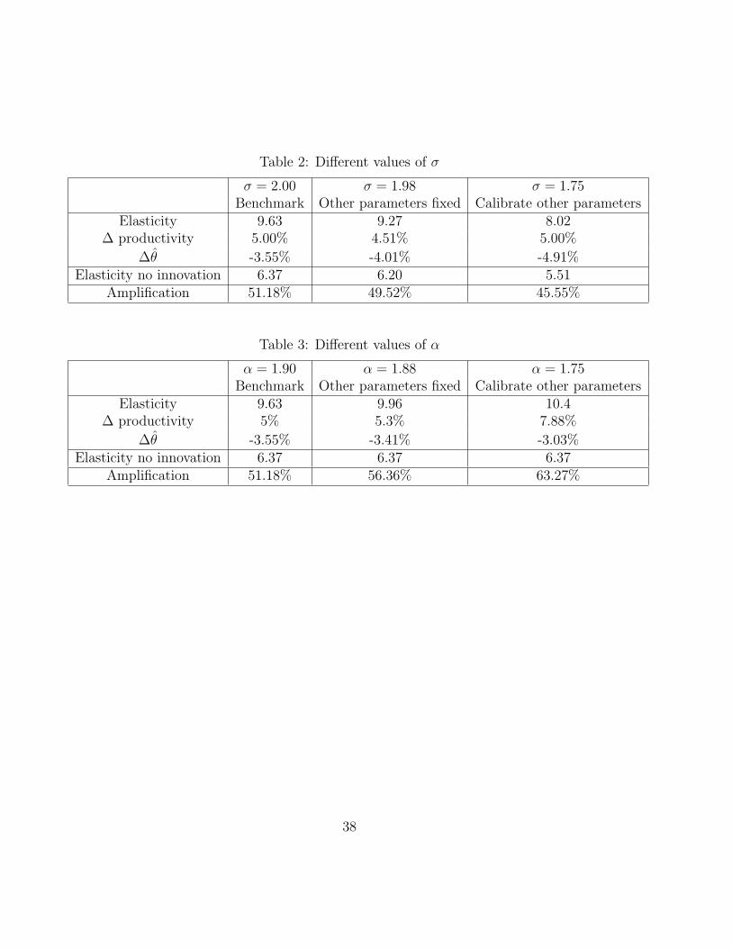
Table 2: Different values of σ
σ = 2.00 σ = 1.98 σ = 1.75Benchmark Other parameters fixed Calibrate other parameters
Elasticity 9.63 9.27 8.02∆ productivity 5.00% 4.51% 5.00%
∆θ -3.55% -4.01% -4.91%Elasticity no innovation 6.37 6.20 5.51
Amplification 51.18% 49.52% 45.55%
Table 3: Different values of α
α = 1.90 α = 1.88 α = 1.75Benchmark Other parameters fixed Calibrate other parameters
Elasticity 9.63 9.96 10.4∆ productivity 5% 5.3% 7.88%
∆θ -3.55% -3.41% -3.03%Elasticity no innovation 6.37 6.37 6.37
Amplification 51.18% 56.36% 63.27%
38
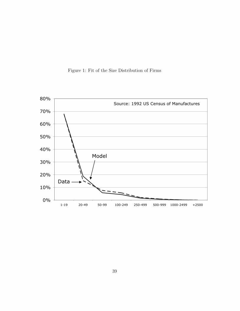
Figure 1: Fit of the Size Distribution of Firms
0%
10%
20%
30%
40%
50%
60%
70%
80%
1-19 20-49 50-99 100-249 250-499 500-999 1000-2499 +2500
Data
Model
Source: 1992 US Census of Manufactures
39
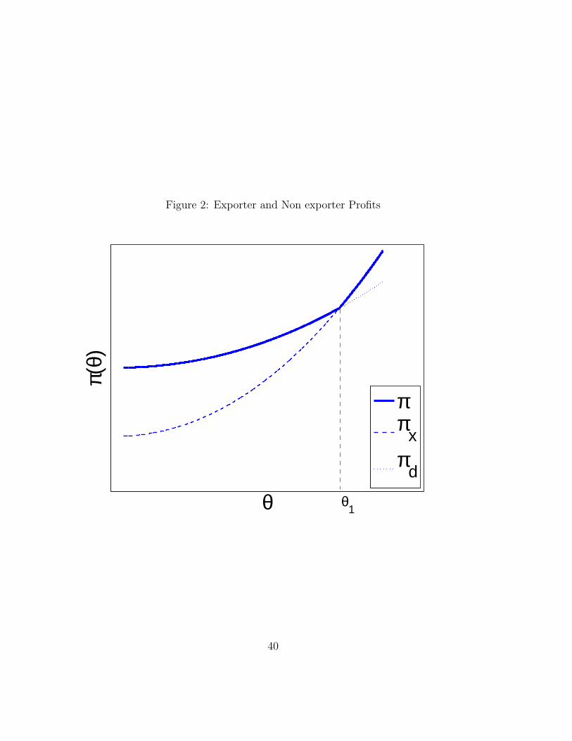
Figure 2: Exporter and Non exporter Profits
θ
π(θ)
ππ
x
πd
θ1
40
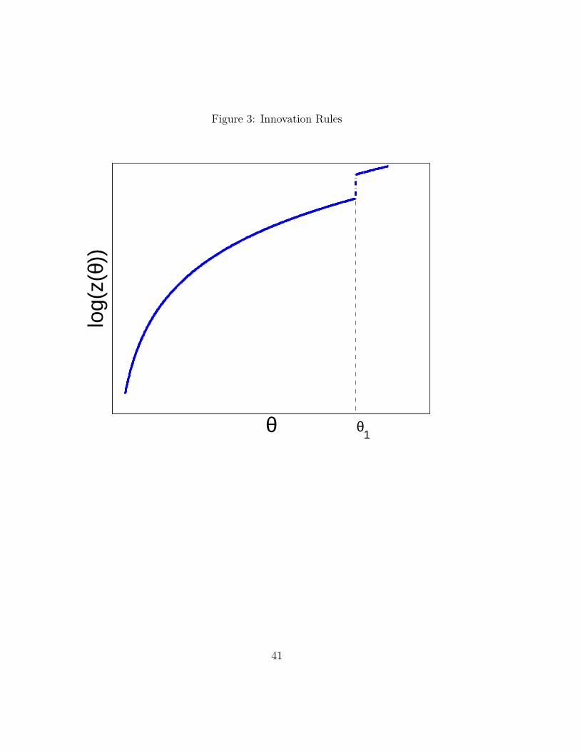
Figure 3: Innovation Rules
θ
log(
z(θ)
)
θ1
41
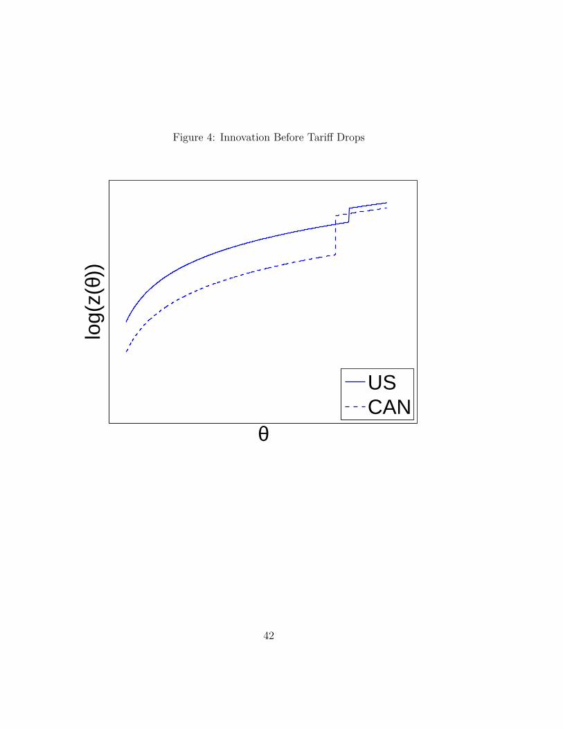
Figure 4: Innovation Before Tariff Drops
θ
log(
z(θ)
)
USCAN
42

Figure 5: US Innovation
θ
log(
z(θ)
)
τ88
τ96
43

Figure 6: CA Innovation
θ
log(
z(θ)
)
τ88
τ96
44

APPENDIX
A Measuring Productivity Increase in the Model
I measure the increase in productivity using chain weighted prices. In the data, real produc-
tivity is measured by calculating current productivity, and deflating it by some price level.
The price level is built by choosing a bundle off goods, and computing the value of that
bundle using current and base period prices.
Denote by period 0 variables those variables in the equilibrium with high tariffs and period 1
variables the low tariff variables. I deflate the productivity increase in current prices by two
price deflators, one that uses period 0 quantities and one that uses period 1 quantities. The
final increase in productivity is a geometric average of the increase using both indices, that
is, a chain weighted productivity increase.
The increase in current price productivity in country i is
∆Prodi =
∫
Ωip1(ω)Q1(ω)dω∫
Ωih1(ω)dω
∫
Ωip0(ω)Q0(ω)dω∫
Ωih0(ω)dω
=w1
w0
(A-1)
where ht(ω) is labor used in production of good ω in period t and Qt(ω) = Q1t(ω) + Q2t(ω)
is total output of good ω in period t.
I deflate ∆Prodi using two price indeces, one using period 0 quantities (Laspeyres price
deflator), and a second one using period 1 quantities (Paasche price deflator). These deflators
are
PL =
∫
Ωip1(ω)Q0(ω)dω
∫
Ωip0(ω)Q0(ω)dω
PP =
∫
Ωip1(ω)Q1(ω)dω
∫
Ωip0(ω)Q1(ω)dω
45
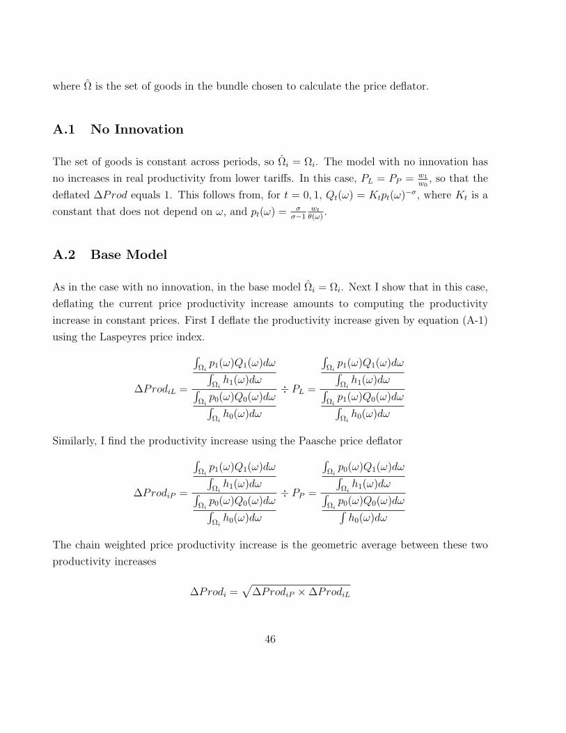
where Ω is the set of goods in the bundle chosen to calculate the price deflator.
A.1 No Innovation
The set of goods is constant across periods, so Ωi = Ωi. The model with no innovation has
no increases in real productivity from lower tariffs. In this case, PL = PP = w1
w0, so that the
deflated ∆Prod equals 1. This follows from, for t = 0, 1, Qt(ω) = Ktpt(ω)−σ, where Kt is a
constant that does not depend on ω, and pt(ω) = σσ−1
wt
θ(ω).
A.2 Base Model
As in the case with no innovation, in the base model Ωi = Ωi. Next I show that in this case,
deflating the current price productivity increase amounts to computing the productivity
increase in constant prices. First I deflate the productivity increase given by equation (A-1)
using the Laspeyres price index.
∆ProdiL =
∫
Ωip1(ω)Q1(ω)dω∫
Ωih1(ω)dω
∫
Ωip0(ω)Q0(ω)dω∫
Ωih0(ω)dω
÷ PL =
∫
Ωip1(ω)Q1(ω)dω∫
Ωih1(ω)dω
∫
Ωip1(ω)Q0(ω)dω∫
Ωih0(ω)dω
Similarly, I find the productivity increase using the Paasche price deflator
∆ProdiP =
∫
Ωip1(ω)Q1(ω)dω∫
Ωih1(ω)dω
∫
Ωip0(ω)Q0(ω)dω∫
Ωih0(ω)dω
÷ PP =
∫
Ωip0(ω)Q1(ω)dω∫
Ωih1(ω)dω
∫
Ωip0(ω)Q0(ω)dω∫
h0(ω)dω
The chain weighted price productivity increase is the geometric average between these two
productivity increases
∆Prodi =√
∆ProdiP × ∆ProdiL
46

A.3 Extensions
In the extensions in section 7, the set of goods produced in each country changes, so I must
take a stance on what the bundle of goods used to compute the price deflator is. I choose
the goods that are produced in both periods as the bundle.
47