innovation and trade policy in a globalized world · innovation and trade policy in a globalized...
TRANSCRIPT
Innovation and Trade Policy in a Globalized World∗
Ufuk AkcigitUniversity of Chicago, NBER, CEPR
Sina T. AtesFederal Reserve Board
Giammario ImpullittiUniversity of Nottingham
November 7, 2017
*** COMMENTS WELCOME ***
Abstract
We assess the effects of import tariffs and R&D subsidies as policy responses to foreigntechnological competition. To this end, we build a dynamic general equilibrium growth modelwhere firm innovation shapes the dynamics of technology endogenously, and, therefore, mar-ket leadership and trade flows, in a world with two large open economies at different stagesof development. The model accounts for competitive pressures exerted by both entrant andincumbent firms. Firms’ R&D decisions are driven by (i) the defensive innovation motive, (ii)the expansionary innovation motive, and (iii) technology spillovers. The theoretical investigationillustrates that, statically, globalization (defined as reduced trade barriers) has ambiguouseffects on welfare, while, dynamically, intensified globalization boosts domestic innovationthrough induced international competition. A calibrated version of the model reproducesthe foreign technological catch-up the U.S. experienced during the 1970s and early 1980s.Accounting for transitional dynamics, we use our model for policy evaluation and computeoptimal policies over different time horizons. The model suggests that the introduction of theResearch and Experimentation Tax Credit in 1981 proves to be an effective policy responseto foreign competition, generating substantial welfare gains in the long run. A counterfac-tual exercise shows that increasing trade barriers as an alternative policy response producesgains only in the very short run, and only when introduced unilaterally, while leading to largelosses in the medium and long run. Protectionist measures generate large dynamic losses fromtrade, distorting the impact of openness on innovation incentives and productivity growth.Finally, we show that less government intervention is needed in a globalized world, thanks toinnovation-stimulating effects of intensified international competition.
Keywords: Economic growth, short and long-run gains from globalization, foreign tech-nological catching up, innovation policy, trade policy, competition.
∗We thank seminar and conference participants at the NBER Summer Institute “International Trade & Investment”and “Macroeconomics and Productivity” groups, Harvard University, Stanford University, University of Pennsylvania,University of Nottingham, Bank of Italy, International Atlantic Economic Society and Italian Trade Study Group,CREST Paris, SKEMA, SED Conference, and CompNet Conference. We also thank Daniel J. Wilson for sharingand helping with his data. Akcigit gratefully acknowledges the National Science Foundation, the Alfred P. SloanFoundation, and the Ewing Marion Kauffman Foundation for financial support. The views in this paper are solelythe responsibilities of the authors and should not be interpreted as reflecting the view of the Board of Governors ofthe Federal Reserve System or of any other person associated with the Federal Reserve System.
Innovation and Trade Policy in a Globalized World
1 Introduction
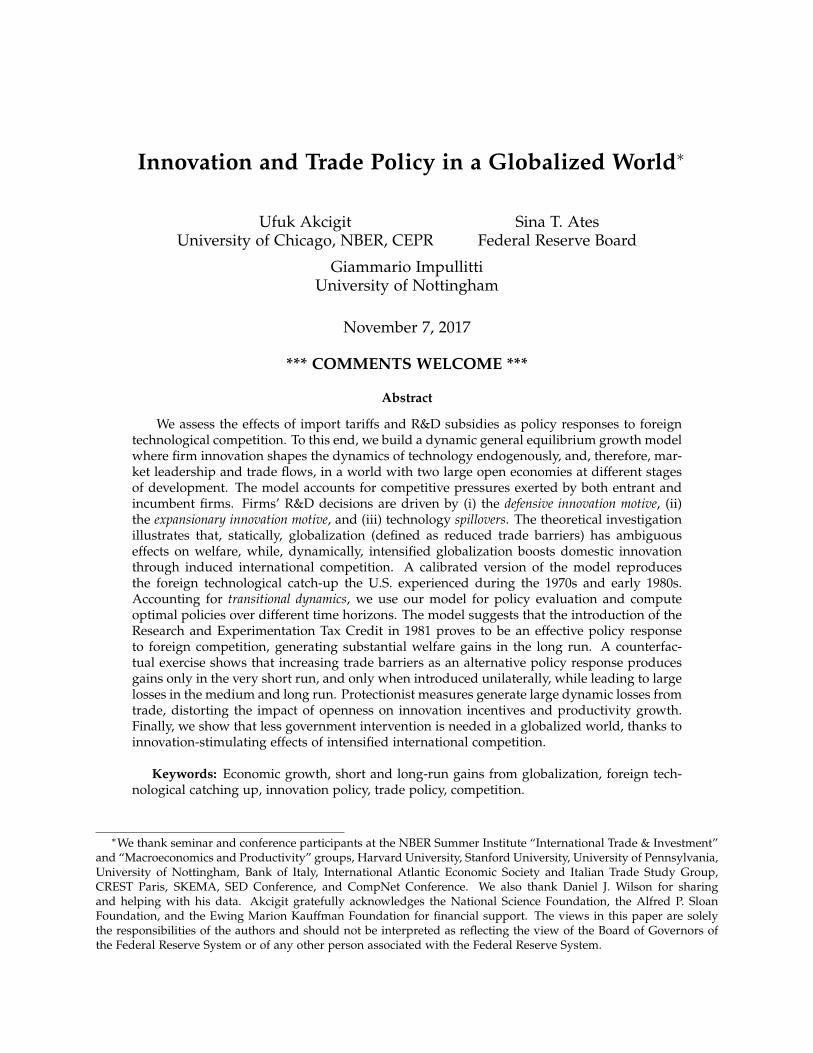
During the past presidential race, a heated debate centered on the position of the U.S. in its traderelationships. President Trump’s speeches focused on the U.S. losing its competitiveness to otherbig players in the world. A favored and widely discussed policy suggestion was raising barriersto international trade. Interestingly, similar concerns were raised also three decades ago, follow-ing the exposure of the U.S. during the 1970s and early 1980s to a remarkable convergence byadvanced countries such as Japan, Germany and France in terms of technology and productivity(see Figure 1). This generated an alarming concern among policy circles, including the Reaganadministration. As opposed to the recent focus on protectionist measures, the Reagan govern-ment, among other policies, introduced an R&D tax credit scheme in 1981 for the first time inU.S. history. In this paper, we evaluate policy responses to international technology competition,focusing on trade and innovation policies. We first provide a new set of empirical facts that areused to motivate the construction of a new dynamic general equilibrium theory of internationaltechnology competition specifically crafted to perform quantitative policy analysis.
Japan
Italy
France
Germany
CanadaUK
US2
4
6
8
Labo
r Pro
duct
ivity
Gro
wth
in M
anuf
actu
ring
(out
put/h
our,
in %
, 197
6−80
avg
.)
−2 2 6 10Growth in Patenting
(Patent Applications in the U.S., in %, 1976−80 avg.)
Figure 1: Convergence between the U.S. and its peers
Notes: The figure shows the relationship between growth of average labor productivity in manufacturing sector and growth inthe number of patent applications for the U.S. and its major trading partners between 1976 and 1980. We obtain data on patentapplications in the U.S. from the USPTO and on international productivity comparisons from Capdevielle and Alvarez (1981).
As illustrated in Figure 1, the U.S. performed poorly relative to its advanced peers in termsof labor productivity and innovation in the second half of the 1970s.1 The average growth inoutput per hours worked in manufacturing was the lowest in the U.S. Moreover, innovation rate,proxied by new patent applications registered in the U.S. by the residents of these foreign coun-
1The relationship over a longer time period is presented in Figure A.5 in Appendix A.3.
2

Innovation and Trade Policy in a Globalized World
tries, expanded substantially except for the U.K. Strikingly, patent applications by U.S. residentshave actually shrunk in absolute terms during the same period. In addition, we find that thelargest growth rates in patent applications have been recorded by those countries whose laborproductivity growth in manufacturing outpaced the U.S. the most. In parallel, U.S. Patent andTrademark Office (USPTO) data show that the ratio of foreign patents to total patents doubledbetween 1975 and 1985.2 While the U.S. held 70 percent of the patent applications in 1975, in 10years this fraction declined to around 55 percent.3
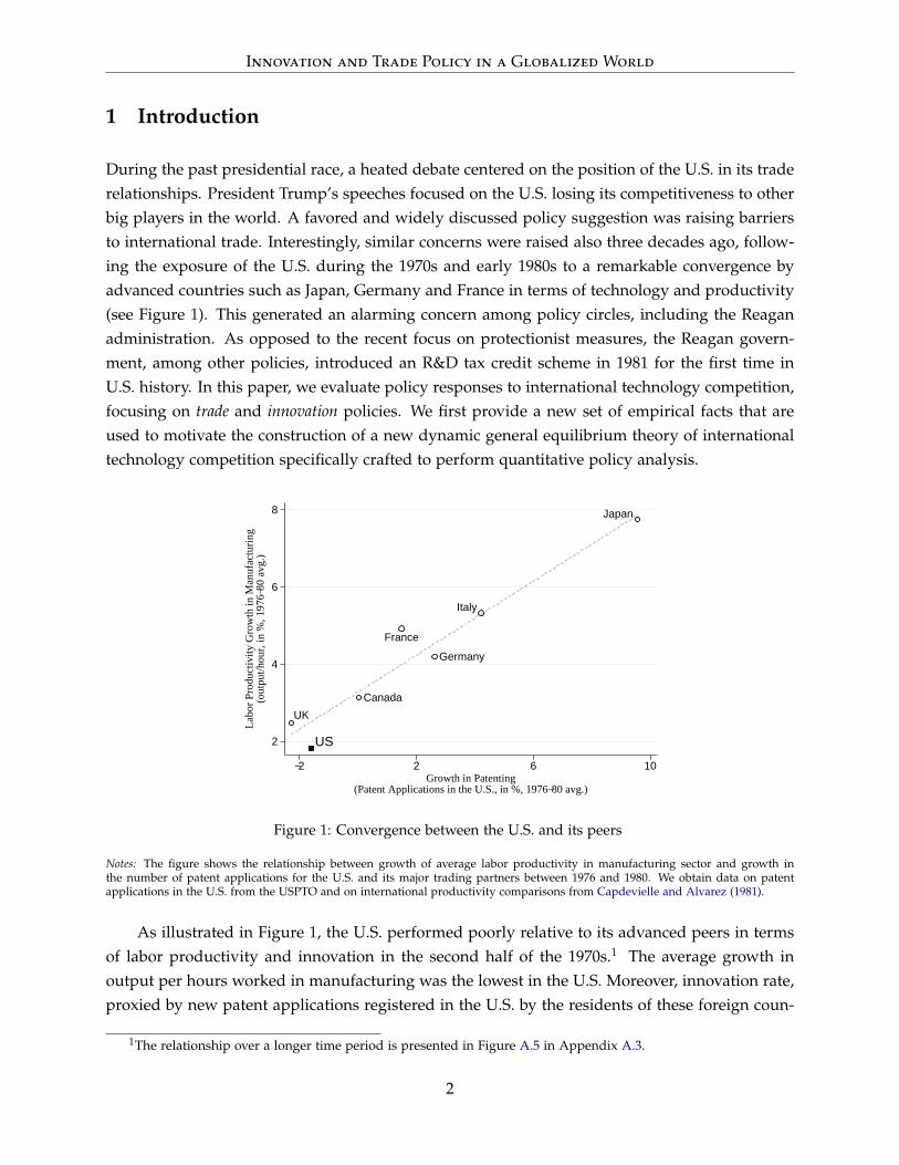
Concerns over U.S. competitiveness in those years led to the introduction of a set of demand-and supply-side policies explicitly targeting incentives for innovation. One of these policies wasthe introduction of the R&D tax credit, both at the federal and state levels. The first federal-levelR&D Tax credit was introduced in 1981. Upon these policy changes, aggregate R&D intensityof U.S. public firms showed a dramatic increase as shown by the solid black line in Figure2a. After the expected delay, the annual share of patents registered by U.S. residents in totalpatent applications picked up as well (see the dashed line in the same figure).4 Starting in1982 with Minnesota, several states followed suit as well and introduced state-level R&D taxcredits, as shown in Figure 2b. By contrast, there was no significant action in R&D policiesof the other major countries, as depicted in Figure 2c.5 Motivated by these facts, this paperprovides a new quantitative investigation of the effects of R&D subsidies in an open economy andcompares them to the effects of raising trade barriers as a response to rising foreign technologycompetition. This policy comparison also allows us to provide new theoretical insights andquantitative perspectives on the gains from globalization.
A sensible quantitative analysis of the economic processes presented above necessitates anopen economy framework where economic growth is shaped by the interplay of innovation andinternational technological competition. Moreover, global R&D races and international trade aredominated by large firms whose choices can affect market aggregates, giving rise to strategicmarket power. The aircraft industry is an example of a technology-intensive sector dominated bytwo firms, Airbus and Boeing, that compete strategically for global market leadership [Irwin andPavcnik (2004), Baldwin and Krugman (1988)]. The top 1 percent of U.S. trading firms accountfor about 80 percent of total U.S. trade and their large market shares allow them to affect marketprices [Bernard et al. (2017), Hottman et al. (2016)]. Hence, a model that allows for strategicinteraction between the competing firms is needed to analyze our facts and to generate newinsights on trade and innovation policies. Moreover, as our facts are intrinsically dynamic, a
2See Figure A.1 in Appendix A.1. This section gives a further account of the empirical findings on internationaltechnological competition and the relevant policies during the period of interest.
3Similar trends are found in countries’ share of global R&D at the sectoral level [see Impullitti (2010)].4Information on sales and R&D expenditures of U.S. public firms are obtained from the COMPUSTAT database.5Following Impullitti (2010), R&D subsidies are calculated using corporate tax data from Bloom et al. (2002),
who take into account different tax and credit systems. The subsidies reflect features of the tax system aimed atreducing the cost of R&D, particularly depreciation allowances and tax credits for R&D expenditures. This structureis responsible for the positive value of our subsidy measure initially. For more details, see Impullitti (2010).
3
Innovation and Trade Policy in a Globalized World
Introduction of federalR&D tax credit (ERTA)
.55
.6
.65
.7
US Share in Total Patents (dashed)
.02
.025
.03
.035
.04R
&D
/Sal
es (s
olid
)
1975 1980 1985 1990 1995Year
a) R&D and innovation intensity of the U.S. firms
MN MN MN MNIAIN
MNIAIN
WVWI
MNIAIN
WVWICA
MNIAIN
WVWICAKSND
MNIAIN
WVWICAKSNDOR
MNIAIN
WVWICAKSNDORIL
MNIAIN
WVWICAKSNDORIL
MA
MNIAIN
WVWICAKSNDORIL
MA
MNIAIN
WVWICAKSNDORIL
MANHCT
MNIAIN
WVWICAKSNDORIL
MANHCTAZMONJRI
MNIAIN
WVWICAKSNDORIL
MACTAZMONJRI
MNIAIN
WVWICAKSNDORIL
MACTAZMONJRIMENC
MNIAIN
WVWICAKSNDORIL
MACTAZMONJRIMENCPA
MNIAIN
WVWICAKSNDORIL
MACTAZMONJRIMENCPAGA
MNIAIN
WVWICAKSNDORIL
MACTAZMONJRIMENCPAGAMTUT
MNIAIN
WVWICAKSNDORIL
MACTAZMONJRIMENCPAGAMTUTMDHIDE
MNIAIN
WVWICAKSNDORIL
MACTAZMONJRIMENCPAGAMTUTMDHIDESCTXID
MNIAIN
WVWICAKSNDORIL
MACTAZMONJRIMENCPAGAMTUTMDHIDESCTXID
MNIAIN
WVWICAKSNDORMACTAZMONJRIMENCPAGAMTUTMDHIDESCTXIDLAVT
MNIAIN
WVWICAKSNDORIL
MACTAZMONJRIMENCPAGAMTUTMDHIDESCTXIDLAVTOH
MNIAIN
WVWICAKSNDORIL
MACTAZMONJRIMENCPAGAMTUTMDHIDESCTXIDLAVTOH
MNIAIN
WVWICAKSNDORIL
MACTAZMONJRIMENCPAGAMTUTMDHIDESCTXIDLAVTOHNE
1 1 13
56
89
1011 11
13
1716
1819
2022
25
28 2829
31 3132
0
10
20
30
Num
ber o
f Sta
tes w
ith T
ax C
redi
t(N
ames
of s
tate
s with
pos
itive
R&
D c
redi
t)
1980 1985 1990 1995 2000 2005Year
Source: Authors’ calculations, Wilson (2009)
b) Number of states
Introduction of R&Dtax credit (ERTA)
Changing the basecalculation
0
.05
.1
.15
.2
.25
Fede
ral/N
ation
al R&
D Su
bsid
y Rate
1980 1985 1990 1995Year
US UK JAP ITA FRA GER
c) Effective R&D tax credit rates across countries
Figure 2: Evolution of R&D credits in the U.S. and other major economies
Notes: Panel A shows the evolution of aggregate R&D intensity (defined as the ratio of total R&D spending over total sales) ofthe public U.S. firms listed in the COMPUSTAT database, and the share of patents registered by the U.S. residents in total patentsregistered in the USPTO database over 1975 to 1995. The ratios are calculated annually. Panel B shows the total number of U.S. stateswith a provision of R&D tax credits, along with their names, for every year since the first adoption of such measure in 1982. PanelC demonstrates effective R&D subsidy rates in the U.S. and its major trading partners over 1979-1995 (unavailable for Canada).
careful policy evaluation needs to take into account the changes along the transition path.
With these key points in mind, we build a new two-country dynamic endogenous growthmodel where innovation determines the dynamics of technology and global market leadership.Our framework builds on the step-by-step innovation models of Schumpeterian creative destruc-tion that allows for strategic interaction among competitors. In both countries, final good firmsproduce output combining a fixed factor and a set of intermediate goods, sourced from domes-tic and foreign producers. In each intermediate sector, a home and a foreign firm compete forglobal market shares and invest in R&D to improve the quality of their product. Free entry by a
4

Innovation and Trade Policy in a Globalized World
fringe of domestic and foreign firms creates an additional source of competitive pressure both onleaders and followers in each product line. International markets are characterized by trade costsand international diffusion of ideas in the form of knowledge spillovers. A theoretical investiga-tion of this setting shows that, statically, openness to trade benefits the fixed factor in the finalgoods production via higher-quality intermediate good imports, which translate into higher pro-ductivity in domestic final good production. By contrast, the effect on business owners, whichoperates through a combination of larger markets size and loss of markets to foreign rivals, isambiguous. In addition, trade openness impacts the economies’ dynamics by affecting motivesfor innovation.
The open economy dimension of our model redefines firms’ incentives to innovate that aretypical of the standard step-by-step models. The key driver of innovation in the generic step-by-step framework is the escape-competition effect, according to which incumbent firms have anincentive to move away from the follower in order to escape competition. A novel implicationof our model is that two such effects arise in a similar spirit. The main difference in an openeconomy with trade frictions is that vertical competition within each product line assumes aninternational dimension, as firms are from different countries. In each line, firms in both coun-tries compete to serve the domestic and foreign market. Innovation generates a ranking of theproduct lines based on the quality/productivity difference between the home firm and the for-eign firm. As in models of trade with firm heterogeneity (e.g. Melitz, 2003), trade costs generatequality cutoffs that partition the product space into exporting and non-exporting firms. But dif-ferently from these models where competition takes place horizontally between firms producingdifferent goods and firms are ranked based on their absolute productivity level, in our modelthe ranking and therefore the cutoffs are pinned down by the productivity of firms relative totheir foreign competitors. When the domestic intermediate good quality is too inferior relative toits foreign counterpart, domestic final good producers decide to source their intermediate goodsfrom abroad, which generates the first import cutoff of the quality. Likewise, if the relative qualityof the domestic producer is above a certain threshold, the foreign final good producer decides toimport from the domestic intermediate good producer, which generates the export cutoff of therelative quality.
The key feature of these two cutoffs is that innovation efforts are intensified around them.Just below the import cutoff, domestic firms exert additional effort to gain their leadership in thehome market; hence, we name it the defensive R&D effort. Likewise, when a domestic firm is justbelow the export cutoff, it exerts additional effort in order to improve its lead and conquer theforeign market. We call this effort the expansionary R&D effort. These two new effects generatea double-peaked R&D effort distribution over the relative quality space that, remarkably, is alsosupported in the USPTO patent data. From a policy point of view, the distinction betweendefensive and expansionary R&D is crucial, as they generate different responses to alternativeindustrial policies, as discussed below.
5
Innovation and Trade Policy in a Globalized World
Another important feature of our model is the free entry of new firms. In both the domesticand foreign economies, new entrants try to replace incumbents. The entry rate is state dependentin that there will be more domestic entry into those sectors where the domestic incumbentsmaintain a larger lead over their foreign rivals. This is another prediction of the model for whichwe find empirical support in the patent data. We observe more patents coming from new entrantsin patent classes where U.S. incumbents have a larger fraction of the patents.
We parameterize the model to match key trade, innovation and growth facts in the late 1970sand reproduce the evolution of global leadership in those years, with the U.S. initially represent-ing the technological frontier in most sectors while a set of European countries plus Japan leadsin a few. The transitional dynamics of the model reproduces the convergence in technologicalleadership observed in the patent data in the 1970s and early 1980s. We validate our model’smechanism with out-of-sample tests concerning the link between innovative activity and techno-logical leadership, and the elasticity of firm-level R&D spending to policy changes. In particular,we lay out striking similarities between the model and the data as to the innovation patterns offirms at different technological positions vis-a-vis their foreign competitors. Furthermore, simu-lating the calibrated model beyond the calibration period, we examine the dynamics of foreigntechnological convergence—a mode of globalization that has not been widely explored in theliterature—in absence of policy interventions. In particular, we demonstrate the significant dete-rioration in the position of U.S. firms in international technological competition that would havearisen in the absence of any policy intervention.
Next, we continue with policy analysis. First, we analyze welfare implications ofprotectionism—i.e., raising trade barriers unilaterally. The welfare implications of the policychange depend on the time horizon over which the policy is evaluated. Increasing the trade costgenerates short-run gains, as it tames international business stealing due to foreign catching-up.These gains more than compensate for the negative effect on aggregate productivity of replacingbetter-quality imported goods with inferior domestic counterparts. Over the first decade after a20 percent increase in trade barriers there are gains up to 0.2 percent of consumption. However,protective measures reduce incentives for domestic firms to do defensive innovation, weakeningthe foreign competitive pressures domestic firms are exposed to. As time goes by, this force dom-inates, leading to substantial drops in welfare in the long run. It operates through the key sourcesof gains from trade in this economy. First, declining defensive innovative effort limits the abilityof the economy to make up for the foregone productivity that would otherwise be generatedby the high-quality imports. Second, it reduces the growth of aggregate profit income. Weakerforeign competition, and the following reduction in defensive innovative activity, generated byprotectionism also shapes the optimal trade policy, calling for a more liberal regime when thewelfare impact is evaluated over a longer time horizon.
As an alternative policy option to protectionism, we feed the model the increase in U.S. R&Dsubsidies that took place in the early 1980s and assess the welfare properties of this policy dur-
6

Innovation and Trade Policy in a Globalized World
ing a period of growing foreign competition. The effective average U.S. R&D subsidy increasesfrom about 5 percent in the 1970s to approximately 19 percent in the post-1981 period. Feedingthe model this subsidy change generates non-negligible gains in both the short and long run.More than three decades after the subsidy increase, consumption is about 0.9 percent higher, andthis gain is driven by both business stealing and innovation. Reducing the cost of innovation,subsidies stimulate both U.S. entrants and incumbent firms’ R&D, thereby accelerating produc-tivity growth and allowing U.S. firms to obtain market leadership. With a 50-year horizon, theconsumption-equivalent welfare gain rises to 1.1 percent per year thanks to the stimulating effectof subsidies on innovation. We also show that the optimal subsidy level for the same horizon ismuch higher than the observed change. In fact, the observed increase in subsidies is an optimalresponse when only a horizon shorter than 10 years is considered, as the growth-stimulatingimpact of subsidies, which becomes stronger over time, calls for higher subsidies over longerhorizons.
Next, we analyze the optimal policy design when both options are available to the policy-maker. A key result is that the direction of the trade policy component crucially depends on theassumption about the response of the trade partners. When the policymaker creates the policyunder the assumption that unilateral changes are possible, the optimal policy favors protectionisttrade measures combined with aggressive R&D subsidies. This is due to the fact that protection-ist policies protect domestic profits yet lower the innovation incentives. Hence, aggressive R&Dsubsidies are needed to make up for the reduced innovation efforts. However, if the trade part-ners retaliate, the optimal policy reverses and calls for a regime as liberal as possible. The risk oflosing the export market plays the key role in this reversal.
Finally, our analysis shows that less policy intervention is needed as the world becomesmore globalized through reduced trade costs. This interesting result is due to the fact that lowertrade costs intensify competition in the global market place. More competitive markets inducemore innovation, both defensive and expansionary. In other words, as globalization takes place,markets take care of the innovation incentives and eliminate the need for policy intervention.
Taking stock, foreign technological catching-up has taken its toll on the technological leader-ship of U.S. firms and led to significant losses in their profits through business stealing. Increas-ing R&D subsidies during periods of accelerating foreign competition proves to be an effectiveresponse to foreign competition, while raising trade barriers generates only small short-run gainsand substantial losses in the long run. The key message of our analysis is that when a countryexperiences fiercer foreign technological competition R&D subsidies help national firms competewithout giving up gains from trade. Finally, optimal trade policy design crucially depends onthe possibility of foreign retaliation, in which case the potential loss of export markets calls for amore liberal trade regime.
7

Innovation and Trade Policy in a Globalized World
Literature Review This paper is related to several lines of research in the literature. The en-dogenous technical change framework that we use as the backbone of our economy is a modelof growth through step-by-step innovation as in Aghion et al. (2001, 2005) and in the latest de-velopments by Acemoglu and Akcigit (2012) and Acemoglu et al. (2016).6 These closed-economymodels are solved in steady state and they abstract from free entry. We propose the first openeconomy version of this class of models, introduce free entry, solve for its transition path andprovide a quantitative exploration of the gains from globalization and the role of innovationsubsidies in open economies.
On modeling the trade side, our setting draws similarities to the theoretical literature thatanalyzes the impact of trade exposure on (industry-level) aggregate productivity in models withheterogeneous firm productivities, pioneered by Melitz (2003).7 Our structural general equilib-rium framework incorporates several forces, such as competition and market size, whose impacton firm innovation is highlighted by recent empirical work that focuses on the nexus of inno-vation and trade [see Muendler (2004), Bustos (2011), Iacovone et al. (2011), Autor et al. (2016),Chen and Steinwender (2016), and, in particular, Bloom et al. (2016) and Aghion et al. (2017),among others].8 It also encompasses technology transfer alongside firm innovation as sources ofproductivity growth, in line with the empirical findings of Cameron et al. (2005). We contributeto this literature by formalizing and quantifying a new theory of endogenous firm decisions andopenness to trade.
Building on the seminal contributions of Rivera-Batiz and Romer (1991) and Grossmanand Helpman (1993), our analysis emphasizes the role of firms’ innovation decisions in shap-ing policy-induced aggregate dynamics and, thus, makes contact with a growing literature ondynamic gains from trade.9 A set of recent papers introduced knowledge diffusion into trademodels as a source that shapes dynamic gains [Perla et al. (2015), Buera and Oberfield (2016),and Sampson (2016), among others]. Impullitti and Licandro (2017), on the other hand, analyzegains from trade in a model of innovation-driven productivity growth with firm heterogene-
6Building on another strand of growth models pioneered by Romer (1990), Grossman and Helpman (1990) usean expanding variety model to analyze the role of international trade and trade policies in determining the long-rungrowth. The adoption of a step-by-step framework instead enables us to study explicitly the strategic interactionbetween firms and its implication for innovation and trade patterns.
7In the fashion of these models, firms with heterogeneous productivities select the markets to serve in our model.Conversely, openness to trade may affect the input-sourcing decisions of firms. For an analysis of this effect in a setupof heterogeneous firms, see Antràs and Helpman (2004).
8 While Bloom et al. (2016) show the positive effect of Chinese import penetration on the technical change in12 European countries, Aghion et al. (2017) examine the differential impact of market size and competition effectson innovation decisions of exporting French firms with heterogeneous initial productivity levels. They find that themarket size effect is the dominant force for firms that have higher productivity at times of increased demand. On arelated note, Mayer et al. (2014) and Mayer et al. (2016) look at the product range and mix of multi-product firms asanother source of within-firm productivity variations. They document the positive effect of increased export marketcompetition on firm productivity through adjustments in these margins.
9In this regard, our attempt advances the literature in the direction pointed out by Burstein and Melitz (2013).In their recent chapter, the authors stress the need for more research dynamic gains from trade, as opposed toextensively-studied static ones, and on the implications of firm and technology dynamics as a potential source.
8
Innovation and Trade Policy in a Globalized World
ity and variable markups. In their analysis of the balanced growth paths, they find that thegrowth effects of trade liberalization doubles the welfare gains obtainable in a static version ofthe model. Analyzing various extensions of the canonical Melitz (2003) framework, Burstein andMelitz (2013) discuss the effects of trade liberalization on firm dynamics. In parallel to our find-ings, they highlight how firms’ innovation responses determine transitional dynamics inducedby trade liberalization. Bloom et al. (2013) develop a trapped-factor model to show that tradeliberalization in a low wage country could reduce the opportunity cost of innovation. Our workcontributes to this literature by emphasizing the role of strategic interaction between firms inshaping their innovation responses, and thereby, the dynamic gains from trade. We also examinethese gains along the transition path, thanks to our framework that is capable of tracking theendogenous evolution of competition and innovation patterns in a tractable fashion. Last butnot least, endogenous productivity growth and transitional dynamics provide further channelsthrough which trade liberalization and policy may affect aggregate welfare, in addition to thoseconsidered by Atkeson and Burstein (2010) and Arkolakis et al. (2012).10
Finally, industrial policies in open economies have been studied by a large body of work.11
Spencer and Brander (1983) and Eaton and Grossman (1986) explore theoretically the strategicmotive to use tariffs and subsidies (to production and innovation) to protect the rents and themarket shares of domestic firms in an imperfectly competitive global economy.12 In a theoreticalsmall open-economy framework of endogenous growth, Grossman and Helpman (1991a) studythe implications of R&D subsidies and industrial policies for optimal long-run growth and wel-fare. Ossa (2015) sets up a quantitative economic geography model to study production subsidycompetition between U.S. states. In the spirit of our work, Impullitti (2010) uses a multi-countryversion of the standard Schumpeterian growth model to assess the welfare properties of R&Dsubsidies in an open economy, although his work is confined to steady state.13 Consideringthe trade policy, Demidova and Rodríguez-Clare (2009) find that an import tariff can be welfareenhancing in a static small open economy with firm heterogeneity and product differentiation.Recently, Costinot et al. (2015) and Costinot et al. (2016) provide intriguing insights on the type-dependent formulation of optimal policy design in static Ricardian and monopolistic competitionenvironments, respectively.14 In contrast to these studies, a distinct feature of our model is the
10Considering a simple model of sequential production in intermediate goods, Melitz and Redding (2014) alsopoint to trade-induced changes in domestic productivity as a source of departure from the findings of Arkolakiset al. (2012), which state that welfare gains from trade in a group of standard models can be derived from a fewaggregate statistics and, accordingly, should be fairly modest. Alessandria and Choi (2014) emphasize the significanceof accounting for transition in this regard.
11Institutional challenges in applying appropriate industrial polices are beyond the scope of this paper. Interestedreaders can see Rodrik (2004) for an extensive discussion.
12See Leahy and Neary (1997) and Haaland and Kind (2008) for recent contributions. While the literature focuseson static models, Grossman and Lai (2004) analyze strategic IPR policy in a multi-country endogenous growth model.
13The paper also relates to the recent quantitative analyzes of R&D subsidies in closed economy. See Acemoglu etal. (2013) and Akcigit et al. (2016a,b).
14 Analyzing trade policies over the business cycle, the recent work by Barattieri et al. (2017) explores the reces-sionary effects of protectionism in a DSGE framework.
9

Innovation and Trade Policy in a Globalized World
link between different modes of foreign competition and innovation at the firm level. We showthat in this setting, different policies affect different types of innovations: For instance, unilateralprotectionism distorts incentives for defensive R&D, whereas retaliation by trade partners distortsincentives for expansionary R&D. This relationship, and the resulting dynamic gains from tradeand transitional dynamics, are central to the design of optimal trade and innovation policy. Dif-ferentiating between the short and long run, we demonstrate the crucial dependence of policyimplications on the horizon considered along the transition.
The rest of the paper is organized as follows. Section 2 introduces the theoretical frameworkand presents analytical results. Section 3 outlines the calibration procedure and provides out-of-sample tests. Section 4 discusses policy implications and optimal policies. Section 5 presentssensitivity and robustness analysis. Finally, Section 6 concludes.
2 Model
In this section, we present a model of international technological competition in which firmsfrom two countries, indexed by c ∈ A, B , compete over the ownership of intermediate goodproduction. Each country has access to the same final good production technology. There is acontinuum of intermediate goods indexed by j ∈ [0, 1] used in final good production. The finalgood is used for consumption, production of intermediate goods and innovation. There is freetrade in intermediate and final good sectors and no trade in assets. Lack of trade in assets rulesout international borrowing and lending and enables the two countries grow at different ratesduring the transition.
In each production line for intermediate goods there are two active firms, one from eachcountry, engaging in price competition to obtain monopoly power of production. The firm thatproduces the variety of better quality after adjusting for the trade cost holds a price advantage.Firms innovate by investing resources to improve the quality of their product in the spirit of step-by-step models. If the quality difference between the products of two firms is large enough, thenthe firm with the leading technology can cover the trade cost and export to the foreign country.Because innovation success is a random process the global economy features a distribution offirms supplying products of heterogeneous quality. In addition to trade in intermediate and finalgoods, there is a second channel of interdependency linking the countries: trade in ideas. Theexchange of ideas consists of technology diffusion through international knowledge spillovers.
In addition to incumbent firms, there is an outside pool of entrant firms. These firms engagein research activity to obtain a successful innovation that enables them to replace the domesticincumbent in a particular product line. Introducing the entry margin allows the model to dis-tinguish the effects of domestic and foreign competition. Understanding these distinct forces isparticularly important once we use our model for the evaluation of different policies.
10

Innovation and Trade Policy in a Globalized World
2.1 Preferences
Consider the following continuous time economy. Both countries admit a representative house-hold with the following CRRA utility:
Ut =∫ ∞
texp(−ρ (s− t))
C1−ψcs − 11− ψ
ds, (1)
where Cct represents consumption at time t, ψ is the curvature parameter of the utility function,and ρ > 0 is the discount rate. The budget constraint of a representative household in country cat time t is
rct Act + Lcwct = PctCct + Act + Tct, (2)
where rct is the return to asset holdings of the household, Lc is the amount of fixed factor (couldbe labor or land) in country c, wct is the fixed factor income, Pct is the price of the consumptiongood in country c, and Tct is the lump-sum tax. Households in country c own all the firms in c;therefore, the asset market clearing condition requires that the asset holdings have to be equal tothe sum of firm values:
Act =∫ 1
0Vcjt + Vcjtdj,
where tilde “˜” denotes values referring to entrant firms. We assume full home bias in assetholding, an assumption that is robustly supported by the empirical evidence in the 1980s and1990s.15
2.2 Technology and Market Structure
2.2.1 Final Good
The final good, which is to be used for consumption, R&D expenditure and the input cost of theintermediate good production, is produced in perfectly competitive markets in both countriesaccording to the following technology:
Yct =Lβ
c
1− β
∫ 1
0qβ
sjtk1−βsjt dj; s ∈ A, B . (3)
Here, Lc is the amount of fixed factor in c, k j refers to the intermediate good j ∈ [0, 1], qj is thequality level of k j, and β is the share of fixed factor in total output. This production functionimplicitly imposes that in each sector j only the highest quality (after adjusting for trade costs)
15For instance, in 1989, 92 percent of the U.S. stock market was held by U.S. residents. Japan, the U.K., France andGermany show similar patterns, at 96 percent, 92 percent 89 percent, and 79 percent, respectively. A similar picturecan be observed until the early 2000s when the home bias started to decline [see, for example, Coeurdacier and Rey(2013)].
11

Innovation and Trade Policy in a Globalized World
intermediate good will be used by the final good producer. Intermediate goods can be obtainedfrom any country, whereas the fixed factor Lc is assumed to be immobile across countries. Wenormalize Lc = 1 in both countries to reduce notation.
Imports of intermediate goods are subject to iceberg trade costs. We assume that in orderto export one unit of an intermediate good, the exporting country needs to ship (1 + κ) units ofthat good, κ > 0. Note that firms in both countries may potentially produce each variety j, andin the absence of trade frictions, they are perfect substitutes after adjusting for their qualities. Asa result, final good producers will choose to buy their inputs from the firm that offers a higherquality of the same variety, once the prices are adjusted to reflect the trade costs. Final goodproducers in both countries have access to the same technology, which will allow us to focus onthe heterogeneity of the intermediate goods sector. Both countries produce the same identicalfinal good, which, under the assumption of frictionless trade in final goods, implies that the priceof the final output in both countries will be the same. We normalize that price to 1 without anyloss of generality.
2.2.2 Intermediate Goods and Innovation
Incumbents. In each product line j, two incumbent firms—one from each country c ∈ A, B—compete for the market leadership à la Bertrand. Each one of these infinitely-lived firms has thesame marginal cost of production η, yet they differ in terms of their quality of output, qcj. We saythat country A is the leader in j if
qAjt > qBjt
and the follower ifqAjt < qBjt.
Firms are in a neck-and-neck position when qAjt = qBjt. The quality qAjt improves through suc-cessive innovations in A or spillovers from B—we will shortly detail the process of spillovers.Each time there is an improvement in country c specific to product line j, the quality increases asfollows:
qcj(t+∆t) = λnt qcjt,
where λ > 1 and nt ∈ N is a random variable, which will be specified below. We assume thatinitially qcj0 = 1, ∀j ∈ [0, 1].
Let us denote by Nt =∫ t
0 nsds the number of quality jumps up to time t. Hence, the qualityof a firm at time t is qcjt = λNcjt . The relative state of a firm with respect to its foreign competitoris called the technology gap between two countries (in the particular product line) and can be
12

Innovation and Trade Policy in a Globalized World
summarized by a single integer mAjt ∈N such that
qAjt
qBjt=
λNAjt
λNBjt= λNAjt−NBjt ≡ λmAjt .
As we shall see, m is a sufficient statistic for describing line-specific values, and, therefore, wewill drop the subscript j when a line-specific value is denoted by m. We assume that there is arelatively large but exogenously given limit in the technology gap, m, such that the gap betweentwo firms is mct ∈ −m, ..., 0, ..., m .
Firms invest in R&D in order to obtain market leadership through improving the quality oftheir products. Let dcj and xcj denote the amount of R&D investment and the resulting Poissonarrival rate of innovation by country c in j, respectively. The production function of innovationstakes the following form:
xcjt =
(γc
dcjt
αcqcjt
) 1γc
.
Note that qcjt in the denominator captures the fact that a quality is more costly to improve if it ismore advanced. This production function implies the following cost function for generating anarrival rate of xcjt :
d(xcjt, qcjt
)= qcjt
αc
γcxγc
cjt. (4)
Entrants. In every product line there are potential entrants from both countries investing ininnovation to enter the market. The innovation technology for entrants is
xcjt =
(γc
dcjt
αcqcjt
) 1γc
.
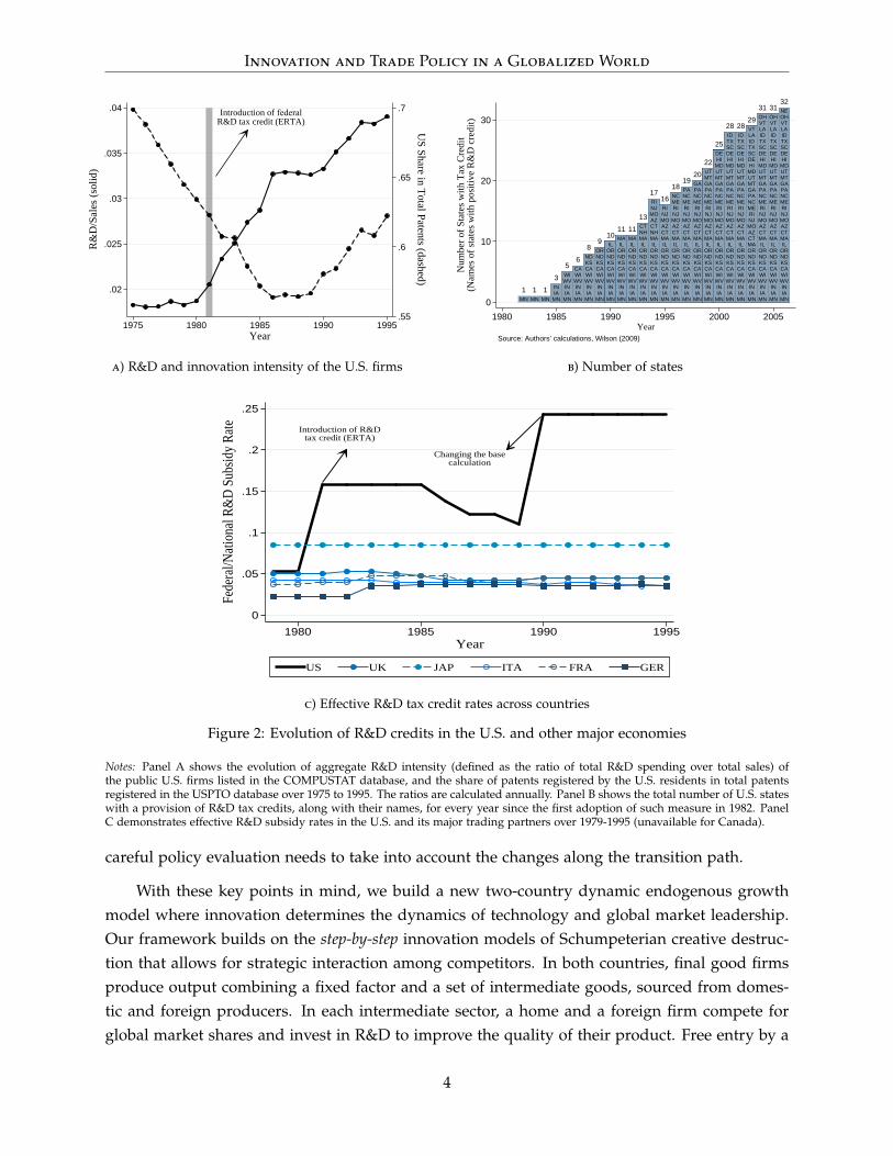
Figure 3 demonstrates the evolution of leadership in intermediate product lines driven byincumbent innovation, entry and exit. In the left panel, five product lines are shown. In thefirst two lines, firms from country B (designated by a square) lead, and in the next two lines,firms from country A (designated by a circle) lead. In the last line, firms are in neck-and-neckposition. Notice that technology gaps are heterogeneous across lines. For instance, in line 1,the incumbent firm from B
(f B1
)leads its competitor from A
(f A1
)by one gap, whereas f B
2
leads f A2 by three gaps. The right panel exhibits how these positions evolve. Country A seizes
technological leadership in the first two lines in two different ways. In line 1, an entrant fromA enters driving the previous incumbent f A
1 out of business. Moreover, it enters with a largeenough quality improvement moving ahead of the previous leader f B
1 . In line 2, f A2 generates an
innovation of a step size larger than three, which enables it to more than close the gap and tocapture the technological leadership. While in line 3 there is no change, in line 4 firms become
13

Innovation and Trade Policy in a Globalized World
neck-and-neck as a result of successful innovation by f B4 . In line 5, an entrant from B brings the
technological leadership to its country while driving out its country’s previous incumbent.
quality, q
productline, j
US FN
line 3line 1 line 2 line 4 line 5
qA1 = qA
2
qB1 = λqA
1
qB2 = λ3qA
2
line 1 line 2 line 4 line 5
entry
entry
a) Product lines
quality, q
productline, jline 3
qA1 = qA
2
qB1 = λqA
1
qB2 = λ3qA
2
line 1 line 2 line 4 line 5
entry
entry
exitexit
b) Entry, exit, and leadership
Figure 3: Evolution of product lines
Notes: Panel A exhibits the positions of competing incumbent firms with heterogeneous quality gaps in a set of product lines.Foreign firms (designated by blue squares) are technological leaders in the firs two lines, U.S. firms (red circle) are leaders in thenext two lines, and firms are in neck-and-neck position in the last line. Panel B illustrates the effects of innovation by incumbentsand entrants and the resulting dynamic of entry, exit, and technological leadership. Empty squares or circles denote the previousposition of firms that innovate or exit.
Lastly, notice that changes in technological leadership may not result in business stealingin existence of trade costs. A firm steals the business of its foreign competitor in two cases:either when a domestic incumbent—which is so technologically laggard that the product it canproduce is imported—improves its quality enough so that the domestic final good producerfinds it profitable to buy the domestic good, or, when a domestic incumbent improves enough topenetrate the foreign market.
Innovations and Step Size. Each innovation improves the relative position of the firm in thetechnological competition. Conditional on innovation, the new position at which the firm willend up is determined randomly by a certain probability mass distribution Fm (·).16 Because themaximum number of gaps is capped by m, there is a different number of potential gaps for eachfirm to reach depending on its current position in the technological competition. For instance, ifa firm is leading by 10 gaps, with a single innovation it can potentially open up the advantage to11, ..., m, whereas for a neck-and-neck firm, an innovation can help it reach 1, ..., m . Hence,the probability mass function that determines the new position, Fm (·), is a function of m. Inorder to keep the model parsimonious we assume that there exists a fixed given distribution
16Conversely, each innovation comes with an associated step size that is randomly generated by some probabilitymass function.
14

Innovation and Trade Policy in a Globalized World
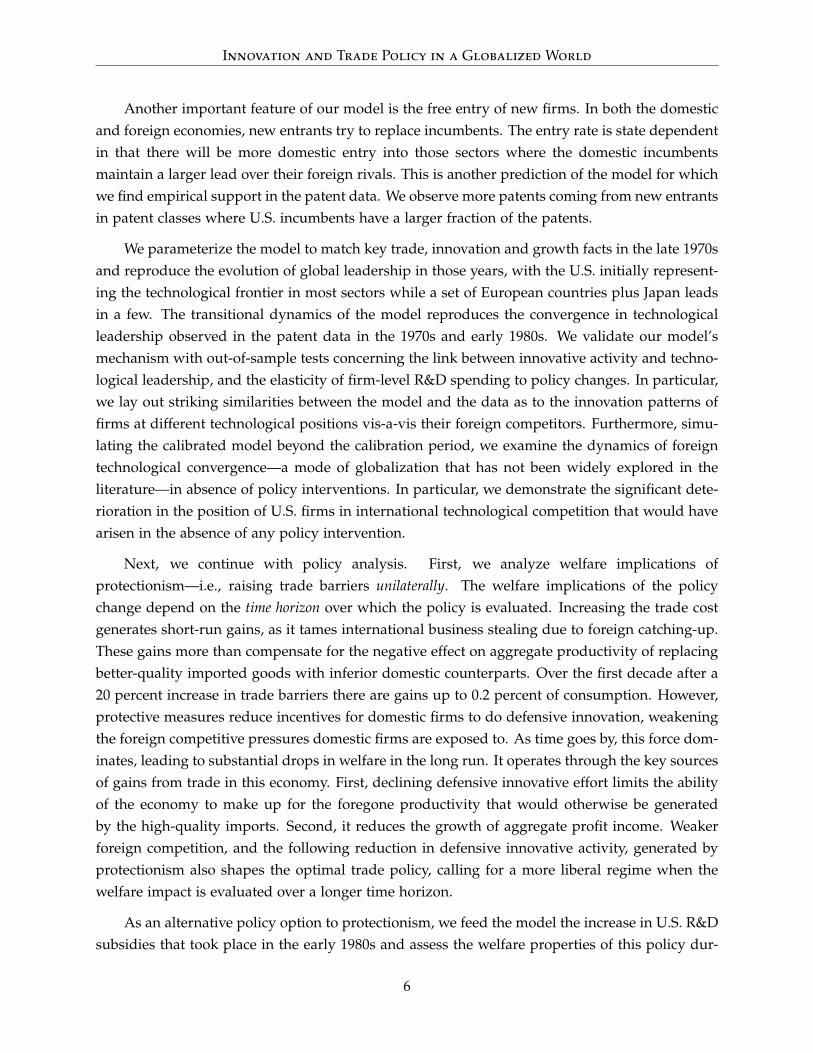
F (·), and we derive Fm (·) from this distribution in the following way. First, we define thebenchmark distribution over positions larger than −m, the most laggard position, as depicted inFigure 4a. We assume that it has the following functional form:
F (n) ≡ c0 (n + m)−φ ∀ n ∈ −m + 1, ..., m . (5)
This parametric structure is defined by only two parameters: a curvature parameter φ > 0 and ashifter c0 that ensures ∑n F (n) = 1. It implies a decaying probability in the new position n. Thisdecay translates into a decay in the probability of an innovation generating larger technologicaljumps.
F
gap size−m + 1 m
F(n) = c0(n + m)−φ
= F−m(n)
−m + 1 m
A
mm + 1
A
Fm(n) ∀n ∈ [m + 1, m]
a) Benchmark
F
gap size
−m + 1 m
−m + 1 m
A
mm + 1
A
Fm(n) ∀n ∈ [m + 1, m]
b) At position m
Figure 4: Probability mass function for new position
Notes: Panel A illustrates the function F (·), defined in equation (5), which we use to generate the position-dependent distributionsof innovation size. Thus, it describes also the probability distribution over potential positions, where an innovation can take the mostlaggard incumbent, denoted by Fm (·). Similarly, Panel B illustrates Fm (·) for a generic position m.
The highest gap size a firm can reach is m. Therefore, the step size distribution specific tothe firm’s position, Fm (·), is defined over positions n ∈ m + 1, ..., m and is derived as follows:
Fm (n) =
F (m + 1) +A (m) f or n = m + 1
F (s) f or n ∈ m + 2, ..., m. (6)
As demonstrated in Figure 4b, A (m) ≡ ∑ms=−m+1 F (s) is an additional probability of improving
15

Innovation and Trade Policy in a Globalized World
the current quality only one more step, on top of what F (·) would imply for that event, whichis given by F (m + 1). This specification for position-specific distributions implies that as firmsbecome technologically more advanced relative to their competitors, it is relatively harder toopen up the gap more than one step at a time. Moreover, their derivation comes at no additionalcost in terms of parameters due to the additive nature of A. Finally, notice that F−m (n) = F (n).
An explanation for this particular way of modeling innovation step sizes is in order. In thebasic step-by-step model, each innovation improves the existing quality of the follower either bya single step or by making the follower catch up with the leader no matter how big the initial gapis. Hence the former is dubbed “slow catch-up regime,” while the latter is dubbed “quick catch-up regime” in Acemoglu and Akcigit (2012). A slow catch-up regime would imply a slow processof convergence in leadership shares, in contrast to what is observed in the data and yet the quickcatch-up regime would have the opposite effect. Therefore, by incorporating F (n), we generalizethis feature and equip the model with enough flexibility to replicate the catch-up process foundin the data.17 The treatment of A (m) in the derivation of position-specific distributions servesthe same purpose. An alternative could involve an equal distribution of the truncated probabilityA (m) across potential positions m + 1, ..., m. This alternative would imply a relatively fatterright tail in Fm (n) and, thus, a higher chance of climbing up the position ladder. However, thisstructure would favor the U.S., most of whose firms are technological leaders in their products,as opposed to the foreign countries, whose firms are lagging in most product lines. Even thougha laggard firm can close the gap by a few steps, a leading firm in this alternative setup couldeasily open up the gap. This happens because for a leading firm, equally distributing A (m)
across a few better positions the firm has ahead means a higher chance of quickly reaching thesepositions again. Given that, in the data, the initial leadership distribution is strongly in favor ofthe U.S., this advantage for the leading firms would result in a shift of the distribution towardslarger gaps, operating against the convergence process in the data.
After a small time interval ∆t → 0, the resulting law of motion for the quality level of anincumbent from A that operates in product line j at position m (−m) can be summarized asfollows:
qAj(t+∆t) =
λnqAjt with probability
(xAjt + xAjt
)Fm (n)∆t for n ∈ m + 1, ..., m
qAjt with probability 1−(xAjt + xAjt
)Fm (n)∆t
qAj(t+∆t) =
λnqAjt with probability
(xAjt + xAjt
)F−m (n)∆t for n ∈ −m + 1, ..., 2m
qAjt with probability 1−(xAjt + xAjt
)F−m (n)∆t
λqAjt with probability(xBjt + xBjt
)Fm (n)∆t
Consider the quality levels associated with the incumbent firms from country A. In a product linewhere the firm from A is in position m, the quality improves if either the domestic incumbent or
17Note that this specification converges to the standard step-by-step model as φ→ ∞.
16

Innovation and Trade Policy in a Globalized World
entrant innovates. Moreover, the quality in a product line where the firm from A is in the highestpossible lag, −m, improves not only if the domestic incumbent and entrant innovates, but alsoif either the foreign incumbent or entrant innovates. The assumption of a maximum number ofgaps implies that, in industries where this maximum is reached, an additional innovation by theleader, despite improving its quality, cannot widen the gap further. The underlying economicintuition is that when the leader at gap m innovates, the technology at gap −m+ 1 becomes freelyavailable to the follower in this product line. Because in this economy the leader and the followerbelong to different countries by construction, this knowledge spillover implies a technology flowacross the countries’ borders. This spillover is a key feature in our economy, generating cross-country convergence in innovation, technology, and income.
2.3 Equilibrium
In this section, we will solve for the Markov Perfect Equilibrium of the model where the strategiesare functions of the payoff relevant state variable m. We will first start with the static equilibrium.Then we will build up the value functions for the intermediate producers and entrants and derivetheir closed form solutions along with the R&D decisions. These will help us characterize theevolution of the world economy over time. Henceforth we will drop the time index t when itcauses no confusion.
Definition 1 (Allocation) An allocation for this world economy consists of interest rate r; country-specific fixed factor price wc; country-specific aggregate output, consumption, R&D expenditure and in-termediate input expenditure Yc, Cc, Dc, Kc; and intermediate good prices, quantities, and innovationarrival rate pj, k j, k∗j , xcj, xcj in country c, product line j.
2.3.1 Households
We start with the maximization problem of the household. The Euler equation of the householdproblem determines the interest rate in the economy as
rct = gctψ + ρ.
2.3.2 Final and Intermediate Good Production
Next, we turn to the maximization problem of the final good producer. Using the productionfunction (3), the final good producers generate the following demand for the fixed factor Lc and
17

Innovation and Trade Policy in a Globalized World
intermediate good j ∈ [0, 1]:
wct =β
1− βLβ−1
c
∫ 1
0qβ
jtk1−βjt dj (7)
pjt = Lβc qβ
jtk−βjt . (8)
Now we consider the intermediate good producers’ problem. In our open economy setting,producers can sell their goods both domestically and internationally. However, as trade is sub-ject to iceberg costs, the producer faces different demand schedules on domestically sold andexported goods. Therefore, the producer earns different levels of profits on these goods depend-ing on the destination country. Let us start with the case of domestic business. We denote theconstant marginal cost of producing an intermediate variety by η. Then, the profit maximizationproblem of the monopolist in product line j becomes
π(qjt)= max
k jt≥0
Lβ
c qβjtk
1−βjt − ηk jt
∀j ∈ [0, 1] .
The optimal quantity and price for intermediate variety j follows from the first order conditions
k jt =
[1− β
η
] 1β
qjt and pj =η
1− β(9)
given that Lc is set to 1. The realized price is a constant markup over the marginal cost and is in-dependent of the individual product quality. Thus, the profit earned by selling each intermediategood domestically is
π(qjt)= πqjt,
where π ≡ ηβ−1
β (1− β)1−β
β β. Notice that in deriving profits, we assumed that the monopolist isable to charge the unconstrained monopoly price. Assumption 1 introduced below ensures thatthe leaders are able to act as unconstrained monopolists.
The problem when selling abroad is different because of the iceberg costs associated withtrade. In line with the trade literature, we define the iceberg cost as the proportional unit to beshipped additionally in order to sell one unit of good abroad. This means that when the firmconsiders meeting the foreign demand it will take into account that its marginal cost will be(1 + κ) η. Given the iceberg costs, only the firm with the higher cost-adjusted productivity willfind it profitable to sell in the other country. Hence, the firm from country A exports intermediategood j to country B if and only if
qAjt
(1 + κ)1−β
β
≥ qBjt.
In this Bertrand competition setting, the existence of a competitor with inferior quality—by def-inition, located in the foreign country—could potentially push the leader to limit pricing. To
18

Innovation and Trade Policy in a Globalized World
simplify the analysis we make the following assumption:
Assumption 1 In every product line, incumbents enter a two-stage game where each incumbent pays anarbitrarily small fee ε > 0 in the first stage in order to bid prices in the second stage.
Assumption 1 implies that only the incumbent with the highest cost-adjusted quality paysthe fee and therefore sets the monopoly price in the second stage. Under this assumption,following similar steps as in the case of domestic sales leads to the following optimal quantityexported and the associated profits:
k∗cjt =
[1− β
(1 + κ) η
] 1β
L f qcjt and p∗j =(1 + κ) η
1− β⇒ π∗
(qjt)= π∗L f qcjt, (10)
with π∗ = ((1 + κ) η)β−1
β (1− β)1−β
β β < π, where the star indicates the equilibrium in the exportmarket.
Figure 5 summarizes the effect of iceberg costs on the technology frontier of two competingcountries.
quality, q
productline, j
US1
US2
US1’
US2’
FN1
FN2FN1’
FN2’
US1 US2 US firms, when sold at home
US1’ US2’ US firms, when sold abroad
Export Domestic sale only Import0 1
Figure 5: Effect of iceberg cost on quality and trade flows
Notes: The figure exhibits the technology frontiers, defined as the product qualities of incumbent firms over all product lines, of twocountries in an example economy (shown by the solid lines). When exporting, the effective technology frontiers (given by the dashedlines) are lower than the actual ones because the exporters need to incur iceberg costs.
Just to fix ideas, in this figure product lines are (re)ordered according to the level of qualitiesin a descending order. The solid lines define the quality frontier of the domestic intermediateproducers, where H and F denote the home and the foreign country, respectively. The dashed
19
Innovation and Trade Policy in a Globalized World
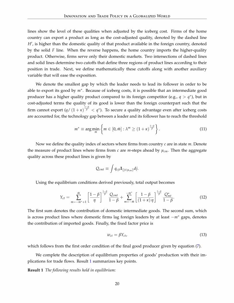
lines show the level of these qualities when adjusted by the iceberg cost. Firms of the homecountry can export a product as long as the cost-adjusted quality, denoted by the dashed lineH′, is higher than the domestic quality of that product available in the foreign country, denotedby the solid F line. When the reverse happens, the home country imports the higher-qualityproduct. Otherwise, firms serve only their domestic markets. Two intersections of dashed linesand solid lines determine two cutoffs that define three regions of product lines according to theirposition in trade. Next, we define mathematically these cutoffs along with another auxiliaryvariable that will ease the exposition.
We denote the smallest gap by which the leader needs to lead its follower in order to beable to export its good by m∗. Because of iceberg costs, it is possible that an intermediate goodproducer has a higher quality product compared to its foreign competitor (e.g., q > q∗), but incost-adjusted terms the quality of its good is lower than the foreign counterpart such that the
firm cannot export (q/ (1 + κ)1−β
β < q∗). To secure a quality advantage even after iceberg costsare accounted for, the technology gap between a leader and its follower has to reach the threshold
m∗ ≡ arg minm
m ∈ [0, m] : λm ≥ (1 + κ)
1−ββ
. (11)
Now we define the quality index of sectors where firms from country c are in state m. Denotethe measure of product lines where firms from c are m-steps ahead by µcm. Then the aggregatequality across these product lines is given by
Qcmt ≡∫
qcjtIj∈µcmdj.
Using the equilibrium conditions derived previously, total output becomes
Yct =m
∑m=−m∗+1
[1− β
η
] 1−ββ Qcmt
1− β+−m∗
∑m=−m
[1− β
(1 + κ) η
] 1−ββ Q∗mt
1− β. (12)
The first sum denotes the contribution of domestic intermediate goods. The second sum, whichis across product lines where domestic firms lag foreign leaders by at least −m∗ gaps, denotesthe contribution of imported goods. Finally, the fixed factor price is
wct = βYct, (13)
which follows from the first order condition of the final good producer given by equation (7).
We complete the description of equilibrium properties of goods’ production with their im-plications for trade flows. Result 1 summarizes key points.
Result 1 The following results hold in equilibrium:
20

Innovation and Trade Policy in a Globalized World
1. The final good price is equalized across countries.
2. When the flow of final goods is accounted for, trade is balanced for both countries.
Proof. See Appendix B.1.
2.3.3 Firm Values and Innovation
This subsection presents equilibrium firm values and innovation decisions.18
Incumbent Firms. We can write the value function for country A’s incumbents:19
rAtVAmt (qt)− VAmt (qt) = maxxAmt
Π (m) qt −
(1− τA
)αA
(xAmt)γA
γAqt
+ xAmt
m
∑nt=m+1
Fm (nt)[VAnt
(λ(nt−m)qt
)−VAmt (qt)
]+ xAmt [0−VAmt (qt)]
+(
xB(−m)t + xB(−m)t
) m
∑nt=−m+1
F−m (nt)[VA(−nt) (qt)−VAmt (qt)
]
where Π (m) is defined as
Π (m) =
πLc + π∗L f i f m ≥ m∗
πLc i f m∗ > m > −m∗
0 i f m ≤ −m∗.
The first line on the right-hand side denotes the operating profits net of R&D costs, where τA isthe R&D subsidy. From the definition of Π (m) we can see that exporting increases the size ofthe market, thereby increasing the incentives to innovate. This is the market-size effect. The secondline denotes the expected gains from innovation. This expectation is over potential new positions.The exact position is determined probabilistically by the step size of innovation. For firms thatare close to their rivals and, thus, feel the competition at its most intense, the innovation effortreflects a dominant incentive for taking over the competitor in order to gain market power. Thisis an escape-competition effect typical of step-by-step innovation models. A distinguishing featureof our model, however, is that this force emerges when rivals are apart by two distinct gapsof technology, instead of a single one as is typical of closed-economy versions. The first caseis when a laggard firm is one-step behind short of beating the foreign exporter and gainingaccess to domestic production. This leads to an intense innovation activity by the laggard firm,
18 In equilibrium, m is a sufficient statistic for firm value. Lemma 1 at the end of this subsection will verify thisresult. Accordingly, we replace subscript j with m unless otherwise necessary.
19The problem for incumbent firms from country B is defined reciprocally.
21
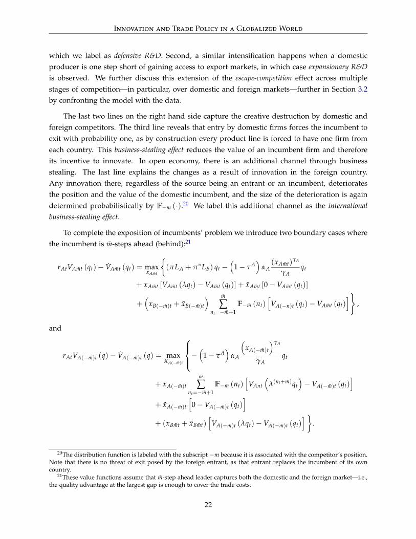
Innovation and Trade Policy in a Globalized World
which we label as defensive R&D. Second, a similar intensification happens when a domesticproducer is one step short of gaining access to export markets, in which case expansionary R&Dis observed. We further discuss this extension of the escape-competition effect across multiplestages of competition—in particular, over domestic and foreign markets—further in Section 3.2by confronting the model with the data.
The last two lines on the right hand side capture the creative destruction by domestic andforeign competitors. The third line reveals that entry by domestic firms forces the incumbent toexit with probability one, as by construction every product line is forced to have one firm fromeach country. This business-stealing effect reduces the value of an incumbent firm and thereforeits incentive to innovate. In open economy, there is an additional channel through businessstealing. The last line explains the changes as a result of innovation in the foreign country.Any innovation there, regardless of the source being an entrant or an incumbent, deterioratesthe position and the value of the domestic incumbent, and the size of the deterioration is againdetermined probabilistically by F−m (·).20 We label this additional channel as the internationalbusiness-stealing effect.
To complete the exposition of incumbents’ problem we introduce two boundary cases wherethe incumbent is m-steps ahead (behind):21
rAtVAmt (qt)− VAmt (qt) = maxxAmt
(πLA + π∗LB) qt −
(1− τA
)αA
(xAmt)γA
γAqt
+ xAmt [VAmt (λqt)−VAmt (qt)] + xAmt [0−VAmt (qt)]
+(
xB(−m)t + xB(−m)t
) m
∑nt=−m+1
F−m (nt)[VA(−n)t (qt)−VAmt (qt)
],
and
rAtVA(−m)t (q)− VA(−m)t (q) = maxXA(−m)t
−(
1− τA)
αA
(xA(−m)t
)γA
γAqt
+ xA(−m)t
m
∑nt=−m+1
F−m (nt)[VAnt
(λ(nt+m)qt
)−VA(−m)t (qt)
]+ xA(−m)t
[0−VA(−m)t (qt)
]+ (xBmt + xBmt)
[VA(−m)t (λqt)−VA(−m)t (qt)
] .
20The distribution function is labeled with the subscript −m because it is associated with the competitor’s position.Note that there is no threat of exit posed by the foreign entrant, as that entrant replaces the incumbent of its owncountry.
21These value functions assume that m-step ahead leader captures both the domestic and the foreign market—i.e.,the quality advantage at the largest gap is enough to cover the trade costs.
22

Innovation and Trade Policy in a Globalized World
The last term in the value function of m-step-behind incumbent captures the knowledgespillovers. When a leader at the maximum gap m innovates, the follower in this sector automat-ically sees its technology jump by a measure λ in order to maintain the maximum gap betweenthe two firms at m. Together with the market-size, escape-competition, and business-stealingeffects described above, the international knowledge spillover is the last key feature driving inno-vation in our framework. In each period the spillover keeps the laggard firms in the innovationrace, preventing them from falling too far behind. Because the innovation technology is the samefor all firms, laggards always have a chance to catch up.
The firms’ problems are characterized by an infinite-dimensional space as a result of thequality levels of intermediate goods. The following lemma renders the firm environment inde-pendent of the current quality of their products.
Lemma 1 The value functions are linear in quality such that Vcm(q) = qvcm for m ∈ −m, ..., m where
rAtvAmt − vAmt = maxxAmt
Π (m)−(1− τA) αA
(xAmt)γA
γA
+xAmt ∑mnt=m+1 Fm (nt)
[λ(nt−m)vAnt − vAmt
]+xAmt [0− vAmt]
+(
xB(−m)t + xB(−m)t
)∑m
nt=−m+1 F−m (nt)[vA(−nt) − vAmt
]
,
This ensures that the firm innovation decision does not depend on j once controlled for m.
Proof. See Appendix B.1.
The first order conditions of the problems defined above yield the following equilibriumcondition for an incumbent in state m:
xcmt =
[
1αc(1−τc) (λ− 1) vcmt
] 1γc−1 i f m = m[
1αc(1−τc) ∑m
n=m+1 Fm (n)
λ(nt−m)vcnt − vcmt
] 1γc−1 i f m < m
.
The equilibrium innovation rates for entrants become
xcmt =
[λvcmt · α−1
c] 1
γc−1 i f m = m[α−1
c ∑mn=m+1 Fm (n) λ(nt−m)vcnt
] 1γc−1 i f m < m
.
Entrants. Lastly, we formulate the entrant problem before defining the equilibrium of the sys-tem. Recall that entry is directed at individual product lines. Every period, a unit mass of en-trepreneurs in each product line attempt to innovate and enter the business. If the entrepreneursucceeds in her attempt, the entrant firm replaces the domestic incumbent; otherwise, the firmdisappears.
23

Innovation and Trade Policy in a Globalized World
An entrant improves on the domestic technology. The problem of an entrant that aims at aproduct line where the current domestic incumbent is m > 0 (m < 0) steps ahead (behind) is asfollows:
Vcmt (qt) = maxxcmt− αc
γc(xcmt)
γc qt + xcmt
m
∑nt=m+1
Fm (nt)Vcnt
(λ(nt−m)qt
), (14)
where Fm (·) denotes the probability distribution of potential step sizes, from which a randomstep will realize conditional on having an innovation. An entrant who fails to innovate exits theeconomy. Solving this problem leads to the following equilibrium value of the entrant firm:
Vcmt (qt) =
(1− 1
γc
)αc (xcmt)
γc qt > 0,
which is independent of the production line’s index j and is determined by the current gap size.
Before finally defining the equilibrium of the model, the government budget constraint canbe written as
Tc = τcm
∑s=−m
αcxγccstQcst, (15)
implying that the total expenditure on subsidies is equal to the lump-sum tax.
Lastly we define the equilibrium.
Definition 2 (Equilibrium) A Markov Perfect Equilibrium of this world economy is an allocation
rc, wc, pj, k j, k∗j , xcj, xcj, Yc, Cc, Dc, Kct∈[0,∞)c∈A,B,j∈[0,1]
such that (i) the sequence of prices and quantities pj, k j, k∗j satisfy (9)-(10) and maximize the operatingprofits of the incumbent firm in the intermediate good product line j; (ii) the R&D decisions
xcj, xcj
maximize the expected profits of firms taking wages wc, aggregate output Yc, the R&D decisions of otherfirms and government policy [τc]t≥0 as given; (iii) labor allocation Lc is the profit maximizing labor choiceof the final good producers; (iv) Yc is as given in equation (12); (v) wages wc and interest rates r clear thelabor and asset markets at every t; and (vi) government budget constraint (15) holds at all times.
Next, we introduce the term for aggregate consumption and the measurement of aggregatewelfare. We leave the analytical discussion of the evolution of the aggregate quantities such asQcmt and Qcmt, which summarize the dynamics of the model, to Appendix B.2.
24
Innovation and Trade Policy in a Globalized World
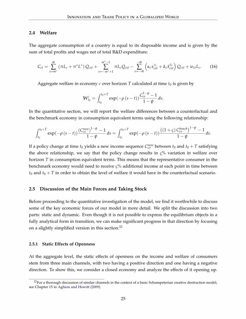
2.4 Welfare
The aggregate consumption of a country is equal to its disposable income and is given by thesum of total profits and wages net of total R&D expenditure:
Cct =m
∑s=m∗
(πLc + π∗L∗) Qcst +m∗−1
∑s=−m∗+1
πLcQcst −−m
∑s=−m
(αcxγc
cst + αc xγccst
)Qcst + wctLc. (16)
Aggregate welfare in economy c over horizon T calculated at time t0 is given by
Wct0=∫ t0+T
t0
exp(−ρ (s− t))C1−ψ
cs − 11− ψ
ds.
In the quantitative section, we will report the welfare differences between a counterfactual andthe benchmark economy in consumption equivalent terms using the following relationship:
∫ t0+T
t0
exp(−ρ (s− t))(Cnew
cs )1−ψ − 11− ψ
ds =∫ t0+T
t0
exp(−ρ (s− t))((1 + ς)Cbench
cs)1−ψ − 1
1− ψds.
If a policy change at time t0 yields a new income sequence Cnewcτ between t0 and t0 + T satisfying
the above relationship, we say that the policy change results in ς% variation in welfare overhorizon T in consumption equivalent terms. This means that the representative consumer in thebenchmark economy would need to receive ς% additional income at each point in time betweent0 and t0 + T in order to obtain the level of welfare it would have in the counterfactual scenario.
2.5 Discussion of the Main Forces and Taking Stock
Before proceeding to the quantitative investigation of the model, we find it worthwhile to discusssome of the key economic forces of our model in more detail. We split the discussion into twoparts: static and dynamic. Even though it is not possible to express the equilibrium objects in afully analytical form in transition, we can make significant progress in that direction by focusingon a slightly simplified version in this section.22
2.5.1 Static Effects of Openness
At the aggregate level, the static effects of openness on the income and welfare of consumersstem from three main channels, with two having a positive direction and one having a negativedirection. To show this, we consider a closed economy and analyze the effects of it opening up.
22For a thorough discussion of similar channels in the context of a basic Schumpeterian creative destruction model,see Chapter 15 in Aghion and Howitt (2009).
25
Innovation and Trade Policy in a Globalized World
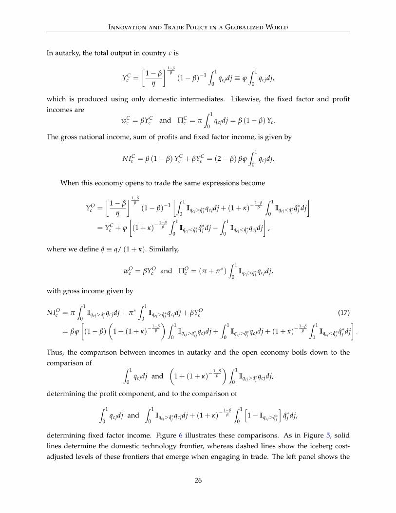
In autarky, the total output in country c is
YCc =
[1− β
η
] 1−ββ
(1− β)−1∫ 1
0qcjdj ≡ ϕ
∫ 1
0qcjdj,
which is produced using only domestic intermediates. Likewise, the fixed factor and profitincomes are
wCc = βYC
c and ΠCc = π
∫ 1
0qcjdj = β (1− β)Yc.
The gross national income, sum of profits and fixed factor income, is given by
NICc = β (1− β)YC
c + βYCc = (2− β) βϕ
∫ 1
0qcjdj.
When this economy opens to trade the same expressions become
YOc =
[1− β
η
] 1−ββ
(1− β)−1[∫ 1
0Iqcj>q∗j qcjdj + (1 + κ)
− 1−ββ
∫ 1
0Iqcj<q∗j q∗j dj
]= YC
c + ϕ
[(1 + κ)
− 1−ββ
∫ 1
0Iqcj<q∗j q∗j dj−
∫ 1
0Iqcj<q∗j qcjdj
],
where we define q ≡ q/ (1 + κ). Similarly,
wOc = βYO
c and ΠOc = (π + π∗)
∫ 1
0Iqcj>q∗j qcjdj,
with gross income given by
NIOc = π
∫ 1
0Iqcj>q∗j qcjdj + π∗
∫ 1
0Iqcj>q∗j qcjdj + βYO
c (17)
= βϕ
[(1− β)
(1 + (1 + κ)
− 1−ββ
) ∫ 1
0Iqcj>q∗cj
qcjdj +∫ 1
0Iqcj>q∗j qcjdj + (1 + κ)
− 1−ββ
∫ 1
0Iqcj<q∗j q∗j dj
].
Thus, the comparison between incomes in autarky and the open economy boils down to thecomparison of ∫ 1
0qcjdj and
(1 + (1 + κ)
− 1−ββ
) ∫ 1
0Iqcj>q∗j qcjdj,
determining the profit component, and to the comparison of
∫ 1
0qcjdj and
∫ 1
0Iqcj>q∗j qcjdj + (1 + κ)
− 1−ββ
∫ 1
0
[1− Iqcj>q∗j
]q∗j dj,
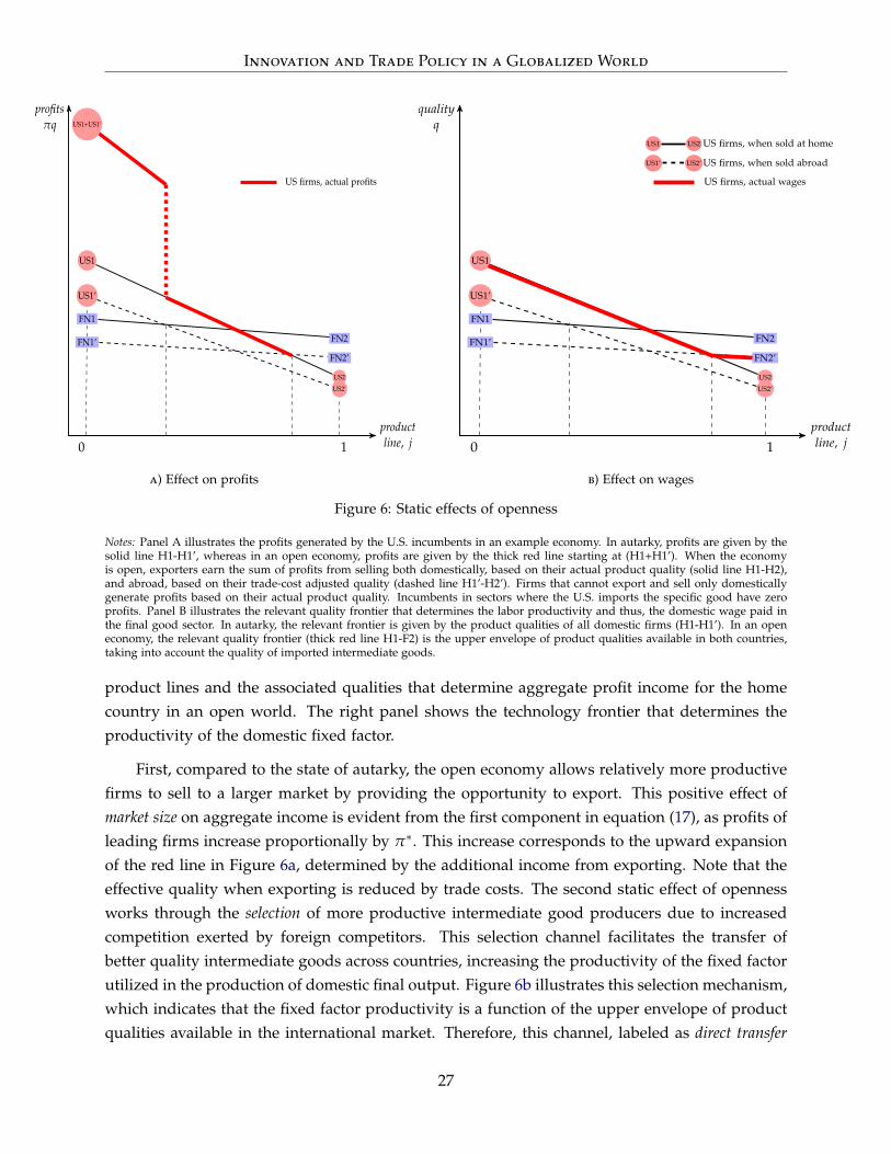
determining fixed factor income. Figure 6 illustrates these comparisons. As in Figure 5, solidlines determine the domestic technology frontier, whereas dashed lines show the iceberg cost-adjusted levels of these frontiers that emerge when engaging in trade. The left panel shows the
26
Innovation and Trade Policy in a Globalized World
profitsπq
productline, j
US1
US2
US1’
US2’
FN1
FN2FN1’
FN2’
0 1
US1+US1’
US firms, actual profits
qualityq
productline, j
US1 US2 US firms, when sold at home
US1’ US2’ US firms, when sold abroad
US firms, actual wages
a) Effect on profits
profitsπq
productline, j
US1
US2
US1’
US2’
FN1
FN2FN1’
FN2’
0 1
US1+US1’
US firms, actual profits
qualityq
productline, j
US1 US2 US firms, when sold at home
US1’ US2’ US firms, when sold abroad
US firms, actual wages
b) Effect on wages
Figure 6: Static effects of openness
Notes: Panel A illustrates the profits generated by the U.S. incumbents in an example economy. In autarky, profits are given by thesolid line H1-H1’, whereas in an open economy, profits are given by the thick red line starting at (H1+H1’). When the economyis open, exporters earn the sum of profits from selling both domestically, based on their actual product quality (solid line H1-H2),and abroad, based on their trade-cost adjusted quality (dashed line H1’-H2’). Firms that cannot export and sell only domesticallygenerate profits based on their actual product quality. Incumbents in sectors where the U.S. imports the specific good have zeroprofits. Panel B illustrates the relevant quality frontier that determines the labor productivity and thus, the domestic wage paid inthe final good sector. In autarky, the relevant frontier is given by the product qualities of all domestic firms (H1-H1’). In an openeconomy, the relevant quality frontier (thick red line H1-F2) is the upper envelope of product qualities available in both countries,taking into account the quality of imported intermediate goods.
product lines and the associated qualities that determine aggregate profit income for the homecountry in an open world. The right panel shows the technology frontier that determines theproductivity of the domestic fixed factor.
First, compared to the state of autarky, the open economy allows relatively more productivefirms to sell to a larger market by providing the opportunity to export. This positive effect ofmarket size on aggregate income is evident from the first component in equation (17), as profits ofleading firms increase proportionally by π∗. This increase corresponds to the upward expansionof the red line in Figure 6a, determined by the additional income from exporting. Note that theeffective quality when exporting is reduced by trade costs. The second static effect of opennessworks through the selection of more productive intermediate good producers due to increasedcompetition exerted by foreign competitors. This selection channel facilitates the transfer ofbetter quality intermediate goods across countries, increasing the productivity of the fixed factorutilized in the production of domestic final output. Figure 6b illustrates this selection mechanism,which indicates that the fixed factor productivity is a function of the upper envelope of productqualities available in the international market. Therefore, this channel, labeled as direct transfer
27
Innovation and Trade Policy in a Globalized World
of technology in Keller (2004), leads to a higher fixed factor income in both countries.23 However,the selection channel implies at the firm level that less productive domestic firms lose the profitsto foreign competitors, which they would earn otherwise in autarky, resulting in a decline ofaggregate profit income. As illustrated in Figure 6a, some product lines fail to generate profits,as they are substituted by imports. Proposition 1 summarizes the static effects of openness.24
Proposition 1 In the simplified environment described above:
A) The static change in income in the open economy relative to autarky is determined by the followingforces: i) exports / market size expansion; ii) technology transfer; iii) import penetration / destructionof laggard firms’ markets. The combined impact of these forces is ambiguous.
B) The static effect of unilateral trade policy liberalization (reduction in tariffs) on aggregate income isdetermined by the second and third channels. Therefore, the direction of its effect is ambiguous.
Proof. See Appendix B.1.
For instance, in an extreme case where a country is lagging in all sectors by a very smallmargin, opening to trade from autarky may decrease national income initially, as the small pro-ductivity gain from transferring slightly better technology may not compensate for the loss ofprofits in all sectors.
2.5.2 Dynamic Effects of Openness and Escape Competition
As explained in Section 2.3.3, market size and selection channels affect not only the aggregatevalues, but also firm decisions, introducing a dynamic component. A larger market size increasesincentives for innovation, whereas the threat of international business stealing, which is the lossof profits to better-quality foreign competitors underlying the selection effect, decreases the valueof a firm. However, an important dynamic channel whose impact is completely absent in a staticcomparison is escape competition, the incentive of firms producing goods of similar qualities toescape foreign competition and gain market dominance. In the remainder, we focus on thisrelatively less standard effect.
In order to emphasize the strategic interaction between intermediate producers introducedby the foreign competition, we focus on a special case of our model. In particular, we considera standard step-by-step open economy setting with two symmetric countries that abstracts fromfirm entry and minimizes the incentives for quality improvements. First, we take αc → ∞ im-plying zero entry in both countries. Second, we assume that λ = 1 + ε where ε is arbitrary closeto zero, implying that quality improvements from innovations are minuscule. Lastly, we also
23Notice that iceberg costs prevent the flow of all better-quality foreign goods available.24Additionally, scale effects arise in a setting where competing countries are of different sizes. For a discussion,
see Chapter 15 in Aghion and Howitt (2009).
28

Innovation and Trade Policy in a Globalized World
abstract from subsidies and trade costs and focus on the balance growth path for the sake ofexposition. In this environment firm values can be written as
rv−m = − x2−m
2+ x−m [v0 − v−m]
rv−m = − x2−m
2+ x−m [v0 − v−m] + xm [v−m−1 − v−m]
rv0 = − x20
2+ x0 [v1 − v0] + x0 [v−1 − v0]
rvm = 2π − x2m2
+ xm [vm+1 − vm] + x−m [v0 − vm]
rvm = 2π − x2m2
+ xm [vm − vm] + x−m [v0 − vm]
with m ∈ 1, ..., m− 1 .25 The following proposition argues that, in this environment, firms inneck-and-neck position have the highest innovation intensity.
Proposition 2 The above assumptions imply that
1. the innovation intensity becomes the highest at neck-and-neck position;
2. the followers innovate at the same intensity and strictly less than the neck-and-neck firms;
3. the leaders do not innovate.
Formally, x0 > x−m = x−m > xm = xm = 0 for m > 0.
Proof. See Appendix B.1.
Proposition 2 formalizes the fact that the positive effect of foreign competitive pressures oninnovation incentives becomes the strongest when firms compete against rivals producing goodsof similar quality. This effect is analogous to the one in closed-economy step-by-step models,but it gains an international aspect in the context of a small open economy. However, notice thatin our general model, the international structure modifies the escape-competition effect in moresubtle ways than merely shifting the origin of the competitive pressure from domestic to foreign.In fact, the intensification of innovation as a result of international competition arises at twopoints in our model instead of one. A combination of market size effect and trade costs drivesthis result. First, firms have an incentive to escape competition for two similar yet distinct reasons:to capture domestic profits and to capture export markets. In both cases, firms attempt to gainmarket power and expand profits; but in the first one, competition is against a foreign exporterover the domestic market, whereas in the second, competition is against a foreign firm over theirdomestic market. Furthermore, because of iceberg trade costs, these challenges do not arise whenactual product qualities are similar, as would happen in the simplified model in Proposition 2.
25Lemma 1 applies also in this environment. For the sake of the argument, we assume that neck-and-neck firmshave zero profits. We also drop country identifiers thanks to symmetry.
29
Innovation and Trade Policy in a Globalized World
Instead, they arise when trade-cost-adjusted qualities are close, which happens at two distinctpositions depending on the market to be captured—i.e., if it is about the domestic market orexports. If the home market is at stake, a laggard home firm tries to escape the competitivepressure exerted by a more advanced foreign competitor, whose product has a similar qualityonce adjusted for trade costs. If an export market is at stake, a relatively more advanced homefirm tries to overcome a laggard foreign firm, whose product quality is competitive once tradecosts are taken into account.
In the analysis above, firm entry was absent in order to highlight the incentives of interest.However, openness can indeed alter entrant incentives through its effect on the value of incum-bents. This is another way that openness affects firm decisions dynamically, as domestic entryleads to the destruction of domestic incumbents, creating a source of underinvestment to innova-tion by incumbents. In Section 3, we remove the restrictive feature of absence of entry, as well asother simplifying assumptions used in this subsection, such as quick catch-up by the followersand zero iceberg costs.
3 Quantitative Analysis
In this section, we study the quantitative implications of our theoretical framework. In particular,we focus on different channels of technological progress and quantify the welfare implicationsof the U.S. R&D policies. We also consider implications of alternative policy options that couldhave been introduced. We start our exploration with the calibration of our model.
3.1 Calibration
When mapping our two-country model to the data, we envision a world that consists of theU.S. and a weighted combination of the following seven countries, which we also employed inthe empirical section: Canada, France, Germany, Italy, Japan, Spain, and the U.K.26 The weightsassociated with each country, listed in Table 1, reflect the count of patents registered in the U.S.by the residents of a specific country in the initial year of the sample (1975) as a fraction of allforeign patents registered in the U.S. in that year.27 In the remainder of this section, country Awill represent the U.S. and country B the foreign country.
As Figures 2c shows, there is a significant break in the R&D policy before and after 1981.Moreover, as shown in Figures A.1 and A.3 in Appendix A.1, there is a strong convergence inthe relative shares of domestic and foreign patents registered in the U.S. as well as in the share
26These are the most innovation-intensive countries competing with the U.S, measured by their share of patentapplications in the USPTO patent data.
27Weights may not sum to 1 due to rounding.
30
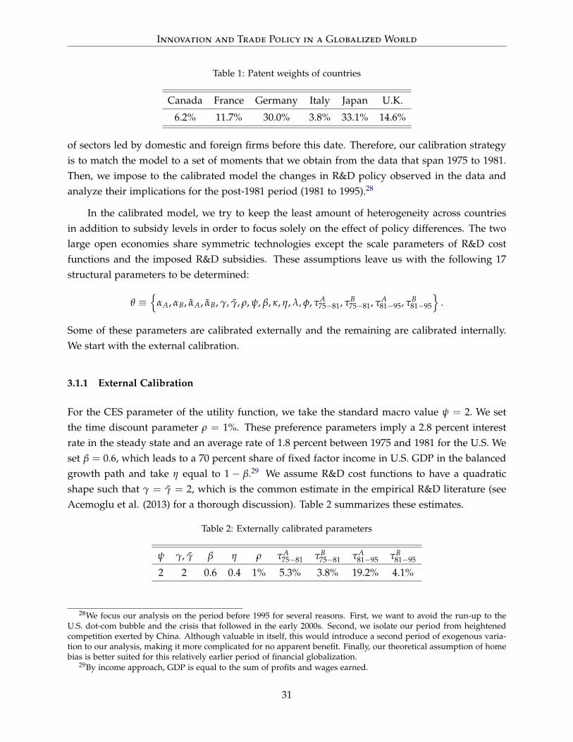
Innovation and Trade Policy in a Globalized World
Table 1: Patent weights of countries
Canada France Germany Italy Japan U.K.
6.2% 11.7% 30.0% 3.8% 33.1% 14.6%
of sectors led by domestic and foreign firms before this date. Therefore, our calibration strategyis to match the model to a set of moments that we obtain from the data that span 1975 to 1981.Then, we impose to the calibrated model the changes in R&D policy observed in the data andanalyze their implications for the post-1981 period (1981 to 1995).28
In the calibrated model, we try to keep the least amount of heterogeneity across countriesin addition to subsidy levels in order to focus solely on the effect of policy differences. The twolarge open economies share symmetric technologies except the scale parameters of R&D costfunctions and the imposed R&D subsidies. These assumptions leave us with the following 17structural parameters to be determined:
θ ≡
αA, αB, αA, αB, γ, γ, ρ, ψ, β, κ, η, λ, φ, τA75−81, τB
75−81, τA81−95, τB
81−95
.
Some of these parameters are calibrated externally and the remaining are calibrated internally.We start with the external calibration.
3.1.1 External Calibration
For the CES parameter of the utility function, we take the standard macro value ψ = 2. We setthe time discount parameter ρ = 1%. These preference parameters imply a 2.8 percent interestrate in the steady state and an average rate of 1.8 percent between 1975 and 1981 for the U.S. Weset β = 0.6, which leads to a 70 percent share of fixed factor income in U.S. GDP in the balancedgrowth path and take η equal to 1− β.29 We assume R&D cost functions to have a quadraticshape such that γ = γ = 2, which is the common estimate in the empirical R&D literature (seeAcemoglu et al. (2013) for a thorough discussion). Table 2 summarizes these estimates.
Table 2: Externally calibrated parameters
ψ γ, γ β η ρ τA75−81 τB
75−81 τA81−95 τB
81−95
2 2 0.6 0.4 1% 5.3% 3.8% 19.2% 4.1%
28We focus our analysis on the period before 1995 for several reasons. First, we want to avoid the run-up to theU.S. dot-com bubble and the crisis that followed in the early 2000s. Second, we isolate our period from heightenedcompetition exerted by China. Although valuable in itself, this would introduce a second period of exogenous varia-tion to our analysis, making it more complicated for no apparent benefit. Finally, our theoretical assumption of homebias is better suited for this relatively earlier period of financial globalization.
29By income approach, GDP is equal to the sum of profits and wages earned.
31

Innovation and Trade Policy in a Globalized World
A crucial set of parameters is the R&D subsidy rates. The numbers we use are those cal-culated in Impullitti (2010), which lack only Canada.30 These data go back to 1979. Given thatthe rates do not fluctuate much for the countries in the sample before the mid-1980s, we take thenumbers before 1979 to be the same as the ones in 1979. For the calibration part, the subsidy ratesfor both countries are 1975-1981 averages, which are again weighted for the foreign countries.When we simulate the model for the post-1981 period, we will recalculate the subsidy rates tomatch the averages across 1982 to 1995. Doing these, we also recalculate the weights of foreigncountries the same way but use 1981 patent counts; the weights are shown in Table 1.
3.1.2 Internal Calibration
We have seven parameters remaining: αA, αB, αA, αB, κ, λ, φ, one of which, φ, determines theshape of the generic step-size distribution. In order to calibrate them, we use six data pointsand the distribution of firms across technology gaps that we derived using USPTO patent data.We start with the discussion of the six moments, summarized in Table 3, that are not related tothe gap distribution. Moments for the foreign country are weighted averages of the values forindividual countries.
The first two moments are the average growth rates of total factor productivity (TFP) in bothcountries, calculated using TFP series in Coe et al. (2009). The next two moments are aggregateR&D as a percentage of GDP, which we obtain using the Main Science and Technology Indicators(MSTI) database of OECD. We use the non-defense R&D intensity numbers, which miss forJapan. However, Science and Engineering Indicators reports of NSF, based on MSTI data, provideestimates of this variable for Japan, which we use to amend our calculations with the OECD data.One issue to note is that MSTI starts in 1981, which is why for this variable we use the values inthis starting year. As a fifth target, we include the birth rate of new establishments for the U.S.computed using the BDS database.31 The sixth moment is the ratio of U.S. manufacturing exportsto GDP, which we derive using World Bank data. These moments allow us to determine sixparameters as follows. Aggregate R&D shares help determine scale parameters of the incumbentR&D cost functions αA, αB . The scale parameter of the entrant R&D cost for country A (αA)
is determined by the U.S. establishment birth rate. Then, TFP growth rates pin down the basicstep size λ and the entrant R&D cost for country B (αB) . Finally, the U.S. export-to-GDP ratiodetermines the iceberg cost κ as κ sets m∗, the minimum gap a firm needs to open up in order toexport, given λ.
The last parameter to be calibrated internally, φ, controls the curvature of the generic prob-ability function over technology gaps, F (n) . As manifested by equations (A.1), this function, by
30We address this issue by recalculating the patent weights after dropping Canada.31We prefer establishment entry instead of firm entry because while in the data firms enter at different sizes, in
our model every firm operates in one product line.
32
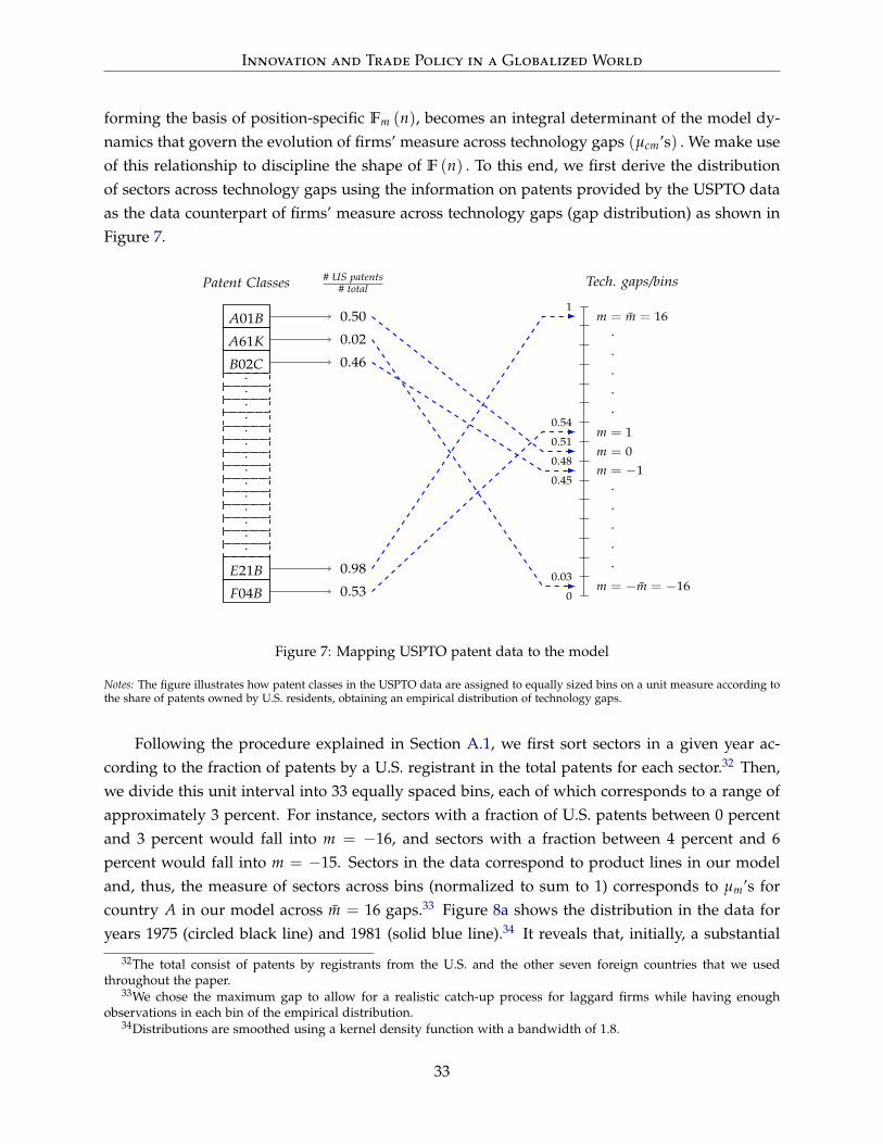
Innovation and Trade Policy in a Globalized World
forming the basis of position-specific Fm (n), becomes an integral determinant of the model dy-namics that govern the evolution of firms’ measure across technology gaps (µcm’s) . We make useof this relationship to discipline the shape of F (n) . To this end, we first derive the distributionof sectors across technology gaps using the information on patents provided by the USPTO dataas the data counterpart of firms’ measure across technology gaps (gap distribution) as shown inFigure 7.
A01B
A61K
B02C··············
E21B
F04B
Patent Classes
400+
clas
ses
400+
sect
ors
0.50
0.02
0.46
0.98
0.53
# US patents# total
·····
·····
m = −m = −160.03
m = −10.48
m = 00.51
m = 10.54
m = m = 161
0
0.45
Tech. gaps/bins
Figure 7: Mapping USPTO patent data to the model
Notes: The figure illustrates how patent classes in the USPTO data are assigned to equally sized bins on a unit measure according tothe share of patents owned by U.S. residents, obtaining an empirical distribution of technology gaps.
Following the procedure explained in Section A.1, we first sort sectors in a given year ac-cording to the fraction of patents by a U.S. registrant in the total patents for each sector.32 Then,we divide this unit interval into 33 equally spaced bins, each of which corresponds to a range ofapproximately 3 percent. For instance, sectors with a fraction of U.S. patents between 0 percentand 3 percent would fall into m = −16, and sectors with a fraction between 4 percent and 6percent would fall into m = −15. Sectors in the data correspond to product lines in our modeland, thus, the measure of sectors across bins (normalized to sum to 1) corresponds to µm’s forcountry A in our model across m = 16 gaps.33 Figure 8a shows the distribution in the data foryears 1975 (circled black line) and 1981 (solid blue line).34 It reveals that, initially, a substantial
32The total consist of patents by registrants from the U.S. and the other seven foreign countries that we usedthroughout the paper.
33We chose the maximum gap to allow for a realistic catch-up process for laggard firms while having enoughobservations in each bin of the empirical distribution.
34Distributions are smoothed using a kernel density function with a bandwidth of 1.8.
33

Innovation and Trade Policy in a Globalized World
mass of U.S. firms are technological leaders, with the mean gap being close to seven; however,subsequently, their distribution has shifted leftward, with the mean gap falling to around fourin 1981. This shift translates into a larger mass of U.S. firms in relatively smaller gap sizes and,therefore, signifies a strong foreign technological catch-up. The calibration of φ aims to matchthe dynamics of this catch-up process that occurred between 1975 and 1981, as described in thediscussion of the model fit below.
In order to obtain the model counterparts of our data targets, we simulate the two economiesbetween 1975 and 1981, initializing the model at the empirical gap distribution in 1975. Initially,we normalize the quality of U.S. intermediate goods to one—i.e., qAj1975 = 1 ∀j.35 We solvethe transition path of the model over 1975 to 1981 as described below. We derive the modelcounterparts of the six moments presented in Table 3 by taking averages of the simulated seriesover the relevant period. We also compute the evolution of the gap distribution in the modelusing equations (A.1) and try to hit the empirical gap distribution in 1981 as the terminal pointof the economy in transition.
-20 -15 -10 -5 0 5 10 15 200
0.01
0.02
0.03
0.04
0.05
0.06
0.07
0.08
0.09
Data = Model US, 1975Data US, 1981Model US, 1981
Technological gaps btw. domestic and foreign firmsa) Technological gap distribution: data and calibration
-20 -15 -10 -5 0 5 10 15 200
0.01
0.02
0.03
0.04
0.05
0.06
0.07
0.08
US
dist
ribu
tion
in 1
981
? = 0:4# ?
? = 0:8# ?
? = 1.37, calibrated
? = 1:2# ?
Technological gaps btw. domestic and foreign firms
b) Identification of φ
Figure 8: Gap distribution after policy changes
Notes: Panel A depicts three technology gap distributions and demonstrates the model’s performance (positive values on the hori-zontal axis denote U.S. technological leadership). The dotted solid line is the empirical distribution in 1975, which also defines theinitial distribution for the model simulation in the calibration. The solid blue line is the empirical distribution in 1981 and definesthe target distribution of the simulation. The dashed red line is the model-generated distribution in 1981, simulated at the calibratedparameters. Panel B illustrates the effect of φ (the curvature parameter of the step-size distribution function) on the simulated gapdistribution, the variation in which enables the identification of φ. It exhibits various model-generated distributions in 1981 thatresult from simulations with varying levels of φ as other parameters being held at their calibrated values.
35The quality levels of firms from B are initialized accordingly with respect to their position in technologicalcompetition. Mathematically, this normalization implies that if in product line j the firm from A is at position m, thenqBj1975 = λ−m, m ∈ −m, ..., m.
34

Innovation and Trade Policy in a Globalized World
Solution Algorithm and Model Fit. In order to solve the model, we first discretize it. Thesolution algorithm assumes that the economy starts in 1975 and transitions to the steady statein T periods, where each period is divided into (∆t)−1 = 25 sub-periods. The algorithm is aniterative backward solution method. The main procedure of the algorithm consists of solving forthe steady state and then deriving the values over the transition period going backward from thesteady state. A brief description follows:36
1. Let M be the set of data moments and Mm be the model counterpart. Define R (M−Mm)
as the objective function that calculates a weighted sum of the difference between data andmodel moments.
2. Guess a set of values for the internally calibrated parameters θguess.
3. Calculate the steady state, where time derivatives are zero by definition. Compute theinnovation rates, the implied growth rates, and finally the steady state interest rates.
4. Next calculate the equilibrium over the transition. Guess a time path for interest rateswith the terminal values being set to steady state at every iteration. Solve for firm valuesand innovation rates backward in time starting from the steady state. Using the resultingsequences, simulate the income path and its growth rate. Use the Euler equation to derivethe implied interest rates and compare them to the series fed initially.
5. Once step 4 converges, use the final interest rate series to compute the aggregate variablesand the model counterparts of the data moments.
6. Minimize R(M−Mm (θguess
))using a minimization routine. We use the sum of squared
errors as the objective function.37
The targeted moments and the model performance in matching these moments are summa-rized in Table 3 and Figure 8a.
Table 3: Model fit
Moment Estimate Target Source
TFP Growth U.S. 0.45% 0.55% Coe et al. (2009)1975-81
TFP Growth FN 2.13% 1.82% Coe et al. (2009) 1975-81
R&D/GDP U.S. 1.65% 1.75% OECD 1981
R&D/GDP FN 1.85% 1.96% OECD 1981
Entry Rate U.S. 10% 10% BDS 1977-81
Export Share U.S. 7.11% 7% WB 1975-81
36A detailed explanation of the steps is presented in Appendix C.2.37The moments that pertain to the gap distribution are weighted by the number of bins matched to make the total
weight of the distribution-related moments the same as the other targets.
35

Innovation and Trade Policy in a Globalized World
Along the transition, the catching-up country grows faster and has higher R&D-to-GDPratios than the leading country. The model captures well these difference between the twoeconomies observed in the data. The entry rate and the export shares are also well fitted. Finally,the position of the dashed line relative to the solid blue one in Figure 8a indicates that the modelperforms well in matching the 1981 distribution of technology gaps. Hence, the cross-countryconvergence mechanism built into the model reproduces the catching up observed in the data.The mechanism in the model is largely governed by the curvature of the step-size distribution,φ, and Figure 8b illustrates how different φ values result in varying shapes of technology gapdistribution. Each line in the figure represents the resulting distribution in 1981, after the modelis simulated at the calibrated parameter values except for different values of φ, starting from1975. Lower values of φ mean a flatter probability distribution F (n) over step sizes (or, equiva-lently, gaps ahead), allowing technologically laggard firms to catch up more quickly. Therefore,a low value of φ would imply a larger leftward shift in the initial distribution of U.S. firms overtechnology gaps. The position of the solid blue line in Figure 8b relative to the circled blackline, which represents the calibration result, illustrates this case. The converse happens for largervalues of φ as demonstrated by the relative position of the yellow dashed line, which is generatedby a value that is 20 percent higher than the calibrated one.
The distribution across new positions, F (n), is the engine of convergence. More precisely,the international knowledge spillover allows laggard firms from the foreign country to stay inthe global innovation race. Importantly, an innovation can generate an improvement of multiplesteps for laggard firms, whereas the number of potential steps to improve becomes smaller as afirm opens up the technological gap with its follower. In Gerschenkron (1962)’s terms, this struc-ture creates an “advantage of backwardness” for followers—i.e., laggard firms have an advantagein the number of steps they can improve with each innovation, while far-ahead leaders cannotopen their lead further quickly. Thus, foreign firms catch up with domestic firms along the tran-sition generating convergence. The cross-country convergence in our economy echoes that inthe Solow model with the key difference that while in Solow convergence is driven by decreas-ing returns in capital accumulation, in our economy knowledge spillovers and an “advantage ofbackwardness" drive the convergence.
Table 4: Internally calibrated parameters
R&D scale R&D scale Step size Iceberg F (n)
αA αB αA αB λ κ φ
0.69 1.14 44.6 8.77 1.49% 19.4% 1.35
The internally calibrated parameters resulting from this procedure are listed in Table 4. Thecombination of the iceberg cost κ and the step size λ imply m∗ = 11—i.e., a firm needs tolead by at least 11 technological gaps to export. The level of φ generates a considerable chance of
36
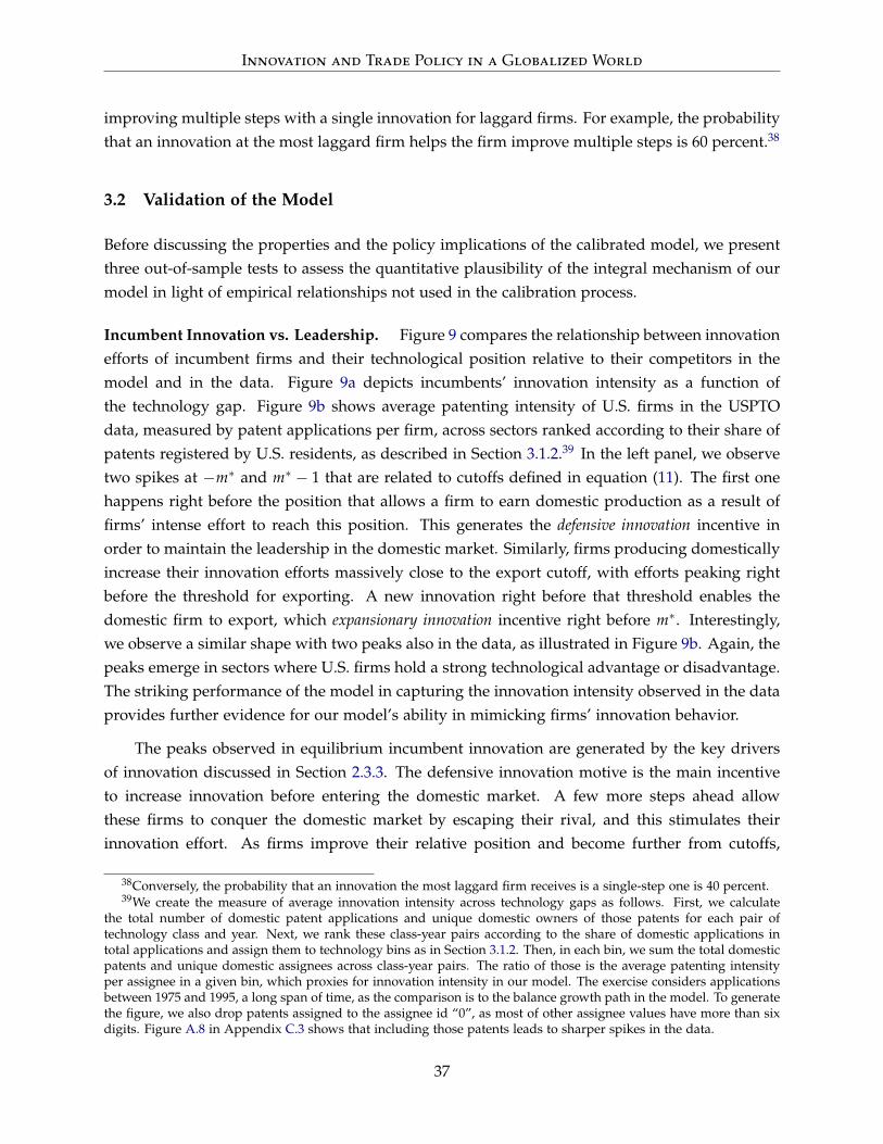
Innovation and Trade Policy in a Globalized World
improving multiple steps with a single innovation for laggard firms. For example, the probabilitythat an innovation at the most laggard firm helps the firm improve multiple steps is 60 percent.38
3.2 Validation of the Model
Before discussing the properties and the policy implications of the calibrated model, we presentthree out-of-sample tests to assess the quantitative plausibility of the integral mechanism of ourmodel in light of empirical relationships not used in the calibration process.
Incumbent Innovation vs. Leadership. Figure 9 compares the relationship between innovationefforts of incumbent firms and their technological position relative to their competitors in themodel and in the data. Figure 9a depicts incumbents’ innovation intensity as a function ofthe technology gap. Figure 9b shows average patenting intensity of U.S. firms in the USPTOdata, measured by patent applications per firm, across sectors ranked according to their share ofpatents registered by U.S. residents, as described in Section 3.1.2.39 In the left panel, we observetwo spikes at −m∗ and m∗ − 1 that are related to cutoffs defined in equation (11). The first onehappens right before the position that allows a firm to earn domestic production as a result offirms’ intense effort to reach this position. This generates the defensive innovation incentive inorder to maintain the leadership in the domestic market. Similarly, firms producing domesticallyincrease their innovation efforts massively close to the export cutoff, with efforts peaking rightbefore the threshold for exporting. A new innovation right before that threshold enables thedomestic firm to export, which expansionary innovation incentive right before m∗. Interestingly,we observe a similar shape with two peaks also in the data, as illustrated in Figure 9b. Again, thepeaks emerge in sectors where U.S. firms hold a strong technological advantage or disadvantage.The striking performance of the model in capturing the innovation intensity observed in the dataprovides further evidence for our model’s ability in mimicking firms’ innovation behavior.
The peaks observed in equilibrium incumbent innovation are generated by the key driversof innovation discussed in Section 2.3.3. The defensive innovation motive is the main incentiveto increase innovation before entering the domestic market. A few more steps ahead allowthese firms to conquer the domestic market by escaping their rival, and this stimulates theirinnovation effort. As firms improve their relative position and become further from cutoffs,
38Conversely, the probability that an innovation the most laggard firm receives is a single-step one is 40 percent.39We create the measure of average innovation intensity across technology gaps as follows. First, we calculate
the total number of domestic patent applications and unique domestic owners of those patents for each pair oftechnology class and year. Next, we rank these class-year pairs according to the share of domestic applications intotal applications and assign them to technology bins as in Section 3.1.2. Then, in each bin, we sum the total domesticpatents and unique domestic assignees across class-year pairs. The ratio of those is the average patenting intensityper assignee in a given bin, which proxies for innovation intensity in our model. The exercise considers applicationsbetween 1975 and 1995, a long span of time, as the comparison is to the balance growth path in the model. To generatethe figure, we also drop patents assigned to the assignee id “0”, as most of other assignee values have more than sixdigits. Figure A.8 in Appendix C.3 shows that including those patents leads to sharper spikes in the data.
37
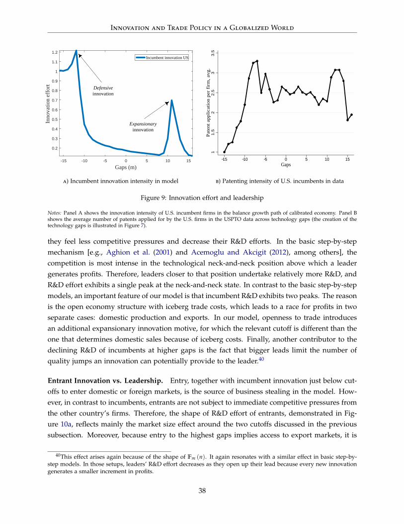
Innovation and Trade Policy in a Globalized World
-15 -10 -5 0 5 10 15
Gaps (m)
0.2
0.3
0.4
0.5
0.6
0.7
0.8
0.9
1
1.1
1.2In
nova
tion
effo
rt Defensive innovation
Expansionary innovation
Incumbent innovation US
a) Incumbent innovation intensity in model
11.
52
2.5
33.
5Pa
tent
app
licat
ion
per f
irm
, avg
.
−15 −10 −5 0 5 10 15Gaps
b) Patenting intensity of U.S. incumbents in data
Figure 9: Innovation effort and leadership
Notes: Panel A shows the innovation intensity of U.S. incumbent firms in the balance growth path of calibrated economy. Panel Bshows the average number of patents applied for by the U.S. firms in the USPTO data across technology gaps (the creation of thetechnology gaps is illustrated in Figure 7).
they feel less competitive pressures and decrease their R&D efforts. In the basic step-by-stepmechanism [e.g., Aghion et al. (2001) and Acemoglu and Akcigit (2012), among others], thecompetition is most intense in the technological neck-and-neck position above which a leadergenerates profits. Therefore, leaders closer to that position undertake relatively more R&D, andR&D effort exhibits a single peak at the neck-and-neck state. In contrast to the basic step-by-stepmodels, an important feature of our model is that incumbent R&D exhibits two peaks. The reasonis the open economy structure with iceberg trade costs, which leads to a race for profits in twoseparate cases: domestic production and exports. In our model, openness to trade introducesan additional expansionary innovation motive, for which the relevant cutoff is different than theone that determines domestic sales because of iceberg costs. Finally, another contributor to thedeclining R&D of incumbents at higher gaps is the fact that bigger leads limit the number ofquality jumps an innovation can potentially provide to the leader.40
Entrant Innovation vs. Leadership. Entry, together with incumbent innovation just below cut-offs to enter domestic or foreign markets, is the source of business stealing in the model. How-ever, in contrast to incumbents, entrants are not subject to immediate competitive pressures fromthe other country’s firms. Therefore, the shape of R&D effort of entrants, demonstrated in Fig-ure 10a, reflects mainly the market size effect around the two cutoffs discussed in the previoussubsection. Moreover, because entry to the highest gaps implies access to export markets, it is
40This effect arises again because of the shape of Fm (n). It again resonates with a similar effect in basic step-by-step models. In those setups, leaders’ R&D effort decreases as they open up their lead because every new innovationgenerates a smaller increment in profits.
38
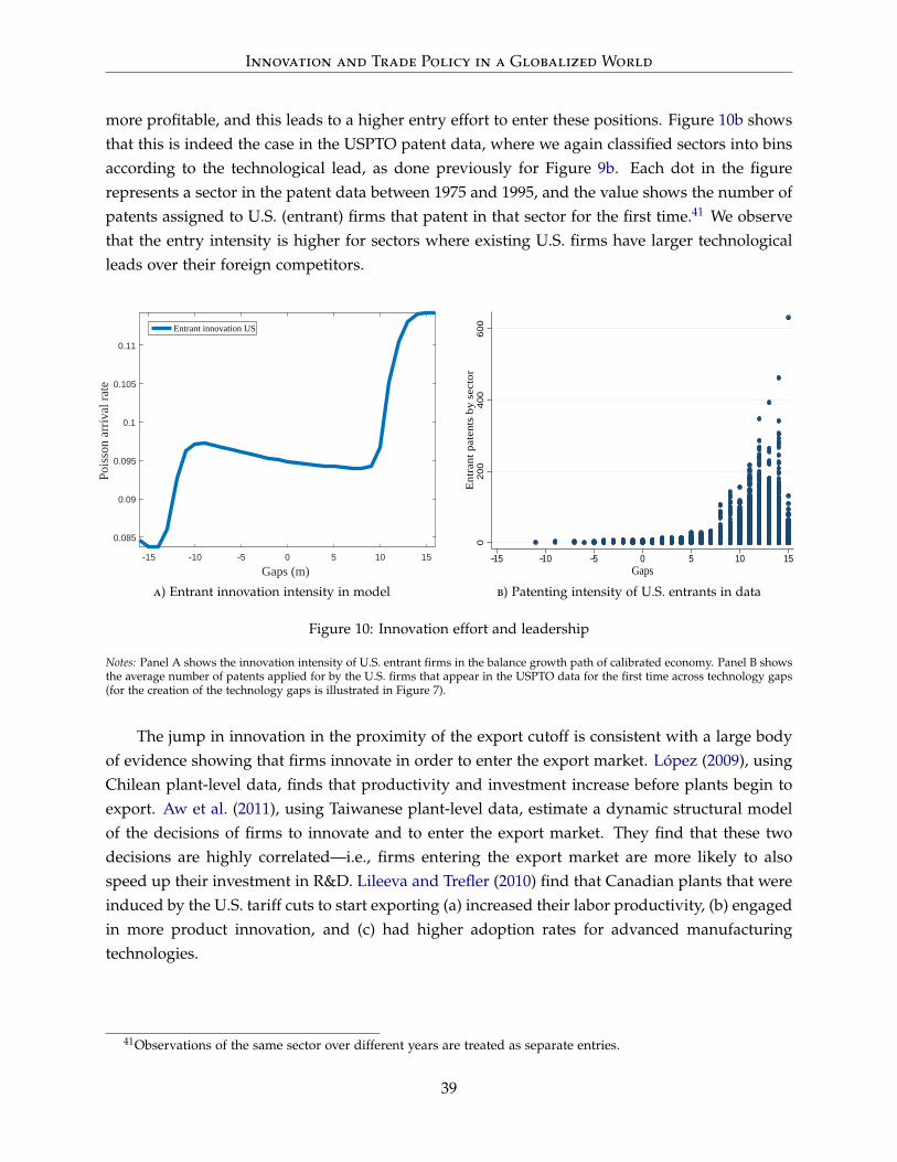
Innovation and Trade Policy in a Globalized World
more profitable, and this leads to a higher entry effort to enter these positions. Figure 10b showsthat this is indeed the case in the USPTO patent data, where we again classified sectors into binsaccording to the technological lead, as done previously for Figure 9b. Each dot in the figurerepresents a sector in the patent data between 1975 and 1995, and the value shows the number ofpatents assigned to U.S. (entrant) firms that patent in that sector for the first time.41 We observethat the entry intensity is higher for sectors where existing U.S. firms have larger technologicalleads over their foreign competitors.
-15 -10 -5 0 5 10 15
Gaps (m)
0.085
0.09
0.095
0.1
0.105
0.11
Pois
son
arri
val r
ate
Entrant innovation US
a) Entrant innovation intensity in model
020
040
060
0E
ntra
nt p
aten
ts b
y se
ctor
−15 −10 −5 0 5 10 15Gaps
b) Patenting intensity of U.S. entrants in data
Figure 10: Innovation effort and leadership
Notes: Panel A shows the innovation intensity of U.S. entrant firms in the balance growth path of calibrated economy. Panel B showsthe average number of patents applied for by the U.S. firms that appear in the USPTO data for the first time across technology gaps(for the creation of the technology gaps is illustrated in Figure 7).
The jump in innovation in the proximity of the export cutoff is consistent with a large bodyof evidence showing that firms innovate in order to enter the export market. López (2009), usingChilean plant-level data, finds that productivity and investment increase before plants begin toexport. Aw et al. (2011), using Taiwanese plant-level data, estimate a dynamic structural modelof the decisions of firms to innovate and to enter the export market. They find that these twodecisions are highly correlated—i.e., firms entering the export market are more likely to alsospeed up their investment in R&D. Lileeva and Trefler (2010) find that Canadian plants that wereinduced by the U.S. tariff cuts to start exporting (a) increased their labor productivity, (b) engagedin more product innovation, and (c) had higher adoption rates for advanced manufacturingtechnologies.
41Observations of the same sector over different years are treated as separate entries.
39

Innovation and Trade Policy in a Globalized World
Credit Elasticity of R&D. The ultimate source of growth in our model is innovation. There-fore, when analyzing the effect of policies on aggregate outcomes, a correct measurement ofthe responsiveness of innovative activity to policy changes is of utmost importance. In orderto evaluate our estimated model’s implications in that regard, we now investigate the empiricalelasticity of innovative activity to R&D credits and compare it with its model counterpart.
In order to measure the credit-elasticity of innovation, we exploit the state-level variationin the dates when credit policies came into action, and conduct a simple firm level regressionanalysis using the COMPUSTAT database. The regression specification is as follows:
ln Yjst = const. + ln Yjst−1 + ln SCst + ψj + ψt + ut , (18)
where ψj and ψt represent firm and year dummies, respectively, and ut is the error term. SCst isthe tax credit level in the state s where firm j operates. For the dependent variable Y we use bothR&D and patent counts. We utilize two different specifications for this regression that differ inthe inclusion of the lagged value of the dependent variable. The results are summarized in Table5. All versions (represented by columns of the table) reveal the positive effect of state level R&Dtax credits on the firms’ innovative activities. This effect is also robust to the existence of laggedvalues of the dependent variable in the regression.42
Table 5: The effect of R&D tax credit on innovation (excl. federal credits)
Dep. Var.:ln(R&Dt) ln(R&Dt) ln(Patentst) ln(Patentst)
(1) (2) (3) (4)
ln(R&Dt−1)- 0.631 - -- (106.67)∗∗∗ - -
ln(Patentt−1)- - - 0.499- - - (72.83)∗∗∗
ln(State creditt)3.153 0.524 2.948 1.203
(10.92)∗∗∗ (2.12)∗∗ (10.93)∗∗∗ (4.28)∗∗∗
Year Dummy Yes Yes Yes Yes
Firm Dummy Yes Yes Yes Yes
Notes: The table lists the results obtained from different OLS specifications that illustrate the effect of (U.S. state-level) tax credits onU.S. firms’ innovation. t-statistics are provided in parenthesis. ∗∗∗,∗∗ ,∗ denote significance at 1 percent,5 percent, and 10 percent,respectively.
The first column of Table 5 shows that, on average, the elasticity of R&D spending withrespect to changes in R&D credit is 3.15. To ensure the quantitative validity of firms’ responseto policy changes in our model, we derive the model counterpart of the same statistic. We
42A version of the regression analysis that also includes the federal credits can be found in Appendix A.2.
40

Innovation and Trade Policy in a Globalized World
first compute the log-difference in R&D expenditure for incumbent firms of country A in eachposition m right before and after the subsidy change from τA
75−81 to τA81−95. Following the same
steps used to create empirical variables, the average elasticity of R&D spending to subsidy isgiven by ∫ 1
0
d log(
αAxγcAj1981qj1981
)d log
(1 + τA
1981
) dj = ∑m
d log(αAxγc
Am1981QAm1981)
log(1 + τA
81−95
)− log
(1 + τA
75−81
) .
This model statistic has a value of 2.27 in contrast to 3.15 in the data. It implies that in the model,an increase in R&D subsidy induces a solid response of R&D expenditure, in line with its empir-ical counterpart, albeit its strength is somewhat weaker than in the data. Note that the empiricaleconomy-wide elasticity is likely to be lower than state-level elasticity due to reallocation of re-sources across states; therefore, it is also reassuring to see that our simulated macro elasticity isbelow the state-level empirical estimate.
3.3 Technological Convergence and Foreign Catching Up
Improvements in a country’s trade partners’ technology is a mode of globalization that has re-ceived less attention in the literature than the reduction of trade and offshoring barriers. Nowwe briefly explore how foreign technological catching-up manifests itself in the leading countryin our model, which again represents the U.S. Figure 11 shows the evolution of the average tech-nological lead that U.S. firms would have over their foreign competitors in the absence of anypolicy intervention.
1975 1980 1985 1990 1995 2000 2005
Years
1
2
3
4
5
6
Mea
n te
chno
logy
gap
of
U.S
. fir
ms
Figure 11: Average technology lead of the U.S. firms, no policy intervention
Notes: the figure exhibits the evolution of The average technology lead that the U.S. firms have over their foreign competitors acrossyears along the transition of the calibrated economy.
41

Innovation and Trade Policy in a Globalized World
The dramatic decline is the symptom of a strong international business-stealing effect,whereby foreign firms progressively capture leadership in more and more markets, and prof-its that were collected by the U.S. firms are now collected by the foreign firms. This business-stealing effect is crucial in shaping the welfare effects of foreign catching-up. In fact, shuttingdown the business stealing by foreign firms by allowing them to improve the quality of theirproducts only up to a step behind the U.S. incumbents generates substantial welfare gains inthe U.S. Concluding that the technological convergence hurt the U.S. economy, we now turn topolicy analysis.
4 Policy Evaluation
In this section we perform a quantitative investigation of various policies and assess their wel-fare implications. We discuss the design of optimal policies considering different horizons forpolicy, also taking into account the transition period. We start the discussion with protectionistmeasures. Then, we continue with R&D policies, analyzing both the observed post-1981 R&Dsubsidy changes and the optimal subsidy levels. We also consider the design of optimal jointpolicy and conclude with a discussion of how retaliation for domestic trade policies by tradepartners can alter the design of optimal policies.
4.1 Protectionist Response
In this subsection, we explore the implications of a unilateral increase in trade barriers as analternative to R&D subsidies and discuss how the optimal tariff policy varies over time hori-zons. Figure 12a shows the consumption-equivalent welfare gains/losses for the representativehousehold generated by a 20 percent rise in the trade cost κ in 1981. Compared to the path ina counterfactual economy that does not experience any policy intervention, protectionism seemsto pay off in the short run, where small gains are generated from the increase in home profits.However, over time, the gains decline and turn negative after two decades.
Digging deeper, unilaterally higher trade barriers generate initially a small increase in profitincome by protecting some sectors from import penetration, shifting market ownership towardhome firms. Recall, though, that the measure of most laggard firms that can benefit from tradeprotection is relatively small for the U.S., as indicated by the left tail of the dashed line in Figure8a. Therefore, the initial gain from laggard firms recapturing production in the domestic marketis limited. Moreover, the replacement of foreign exporters by the laggard home firms means thatthe high-quality foreign products are foregone and replaced by inferior domestic alternatives.This foregone intermediate good quality leads to significant welfare losses. Overall, the combinedwelfare effect is nevertheless positive over the short- to medium run.
42

Innovation and Trade Policy in a Globalized World
10 20 30 40 50 60 70 80 90 100
Time Periods
-0.5
-0.4
-0.3
-0.2
-0.1
0
0.1
0.2
Perc
enta
ge
Protection
a) Consumption equivalent welfare
-15 -10 -5 0 5 10 15
Gaps (m)
0.2
0.3
0.4
0.5
0.6
0.7
0.8
0.9
1
1.1
1.2
Inno
vatio
n ef
fort
Incumbent innovation USProtectionism
b) Innovation response to protectionism
Figure 12: Welfare effects of protectionism: unilateral 20 percent increase in trade barriers
Notes: The figure illustrates the effects of a unilateral 20 percent increase in U.S. trade barriers (protectionist U.S. policy withoutretaliatory response). Panel A shows the welfare change in consumption equivalent terms over different time horizons. Panel Bshows the shift in the innovation-effort profile of U.S. incumbent firms over technology gaps.
As time passes, the factor that governs variations in welfare is the decline in competitivepressures on domestic firms, which leads to a drop in innovative activity. Figure 12b shows thatinnovation efforts of most laggard U.S. firms decrease substantially. Because the protectionistpolicy shifts the threshold for losing the domestic market to a foreign competitor to the left,more firms move further from such an immediate threat. This weaker defensive innovationmotive leads to less innovation by these firms, making it harder to compensate for the loss ofimported frontier technology. Moreover, most U.S. firms, being either exporters or solid domesticproducers that are technologically close to or ahead of their competitors, are not affected byimport protection. As shown in Figure 12b, innovation decisions of this large group of firmsbarely change, implying that they do not contribute any additional boost to profit income orfactor productivity in response to the policy move.43 All in all, the short-run gains from profitsare subdued over time by the loss of foreign technology, while weaker defensive innovationincentive leads to less domestic innovation and, thus, to a slower growth of productivity andprofit income.
The negative relationship between the aggregate innovation effort and protection plays animportant role also for the design of optimal tariff policy. As shown in Figure 13a, the optimaltariff policy, where the U.S. sets the tariffs that imported goods are subject to unilaterally, iseffectively to close the borders to imports, when the relevant horizon over which the policymakercalculates the welfare is very short, such as a decade. However, the preferred level of tariffsdecreases as the relevant horizon becomes longer and suggests a more liberal tariff regime with
43Evidently, the time path of the average technology lead of the U.S. firms is lower than the one in the “no-intervention” case (see Figure A.7a in Appendix C.3).
43

Innovation and Trade Policy in a Globalized World
10 20 30 40 50 60 70 80 90 100
Horizon in years
0.2
0.4
0.6
0.8
1
1.2
1.4
Opt
imal
tari
ff r
ate
(in
mul
tiple
s of
5)
a) Optimal tariff policy over time horizons
0.5 0.6 0.7 0.8 0.9 1 1.1 1.2 1.3 1.4 1.5
Tariff rate (in multiples of 5)
0.1
0.12
0.14
0.16
0.18
0.2
0.22
0.24
Ave
rage
inno
vatio
n in
tens
ity
IncumbentEntrant
b) Average innovation over openness
Figure 13: Optimal tariff policy and innovation over openness
Notes: Panel A shows the optimal unilateral tariff policy for the U.S. over various policy horizons. On the vertical axis, (1 + x)implies x% higher (lower) trade cost relative to the calibrated value for values of x larger (smaller) than zero. Panel B shows thenegative effect of unilaterally higher U.S. tariff rates on average innovation intensity of both entrant and incumbent U.S. firms, with1 denoting the calibrated tariff rate.
respect to the calibrated economy when the horizon considered extends beyond two decades. AsFigure 13b demonstrates, the reason is the dampening effect of higher tariff rates imposed by thehome country on domestic aggregate innovation. This dynamic negative effect dominates staticgains over time and, therefore, implies lower tariffs for optimal policy when longer time horizonsare considered.
4.2 R&D Subsidies
As a result of the policy intervention to improve the competitiveness of U.S. companies, the levelof R&D subsidies in the U.S. increased significantly from an average of 5.1 percent in the pre-1981 period to an average of 19.2 percent in the subsequent period, while the foreign subsidyremained fairly constant at 3.8 percent and 4.1 percent in the respective periods. Figure 14 showsthe effect of the subsidy on the post-1981 distribution of technology gaps. On both panels, themodel gap distribution in 1981, which is closely calibrated to data in 1981, is the solid blue line.In the benchmark economy, which experiences no policy intervention, the transition leads to thedashed line in the left panel by the year 1995. By contrast, in the economy where subsidies wereintroduced instead in 1981, the resulting distribution in 1995 just becomes the solid blue line inthe right panel. The effect of higher subsidies is a small shift to the right relative to the dashedline, which represents the no-intervention case.44
44In the right panel, the circled line shows the drastic shift that would have arisen had the optimal level of R&Dsubsidy been introduced in 1981. We will discuss optimal subsidies in the next subsection.
44
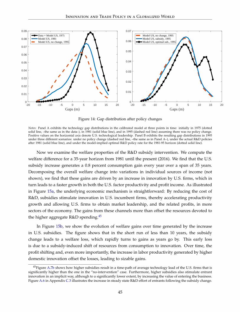
Innovation and Trade Policy in a Globalized World
-20 -15 -10 -5 0 5 10 15 20
Gaps (m)
0
0.01
0.02
0.03
0.04
0.05
0.06
0.07
0.08
0.09
Data = Model US, 1975Model US, 1981Model US, no change, 1995
-20 -15 -10 -5 0 5 10 15 20
Gaps (m)
0
0.01
0.02
0.03
0.04
0.05
0.06
0.07
Model US, no change, 1995Model US, subsidy, 1995Model US, optimal sub., 1995
Figure 14: Gap distribution after policy changes
Notes: Panel A exhibits the technology gap distributions in the calibrated model at three points in time: initially in 1975 (dottedsolid line, –the same as in the data–), in 1981 (solid blue line), and in 1995 (dashed red line) assuming there was no policy change.Positive values on the horizontal axis denote U.S. technological leadership. Panel B exhibits the resulting gap distributions in 1995under three different scenarios: under no policy change (dashed red line, –the same as in Panel A–), under the actual R&D policiesafter 1981 (solid blue line), and under the model-implied optimal R&D policy rate for the 1981-95 horizon (dotted solid line).
Now we examine the welfare properties of the R&D subsidy intervention. We compute thewelfare difference for a 35-year horizon from 1981 until the present (2016). We find that the U.S.subsidy increase generates a 0.8 percent consumption gain every year over a span of 35 years.Decomposing the overall welfare change into variations in individual sources of income (notshown), we find that these gains are driven by an increase in innovation by U.S. firms, which inturn leads to a faster growth in both the U.S. factor productivity and profit income. As illustratedin Figure 15a, the underlying economic mechanism is straightforward: By reducing the cost ofR&D, subsidies stimulate innovation in U.S. incumbent firms, thereby accelerating productivitygrowth and allowing U.S. firms to obtain market leadership, and the related profits, in moresectors of the economy. The gains from these channels more than offset the resources devoted tothe higher aggregate R&D spending.45
In Figure 15b, we show the evolution of welfare gains over time generated by the increasein U.S. subsidies. The figure shows that in the short run of less than 10 years, the subsidychange leads to a welfare loss, which rapidly turns to gains as years go by. This early lossis due to a subsidy-induced shift of resources from consumption to innovation. Over time, theprofit shifting and, even more importantly, the increase in labor productivity generated by higherdomestic innovation offset the losses, leading to sizable gains.
45Figure A.7b shows how higher subsidies result in a time-path of average technology lead of the U.S. firms that issignificantly higher than the one in the “no-intervention” case. Furthermore, higher subsidies also stimulate entrantinnovation in an implicit way, although to a significantly lower extent, by increasing the value of entering the business.Figure A.6 in Appendix C.3 illustrates the increase in steady state R&D effort of entrants following the subsidy change.
45
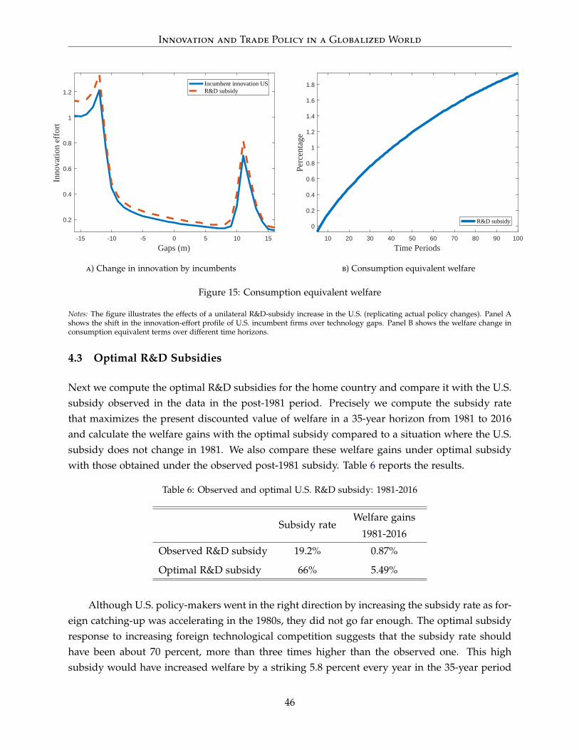
Innovation and Trade Policy in a Globalized World
-15 -10 -5 0 5 10 15
Gaps (m)
0.2
0.4
0.6
0.8
1
1.2
Inno
vatio
n ef
fort
Incumbent innovation USR&D subsidy
a) Change in innovation by incumbents
10 20 30 40 50 60 70 80 90 100
Time Periods
0
0.2
0.4
0.6
0.8
1
1.2
1.4
1.6
1.8
Perc
enta
ge
R&D subsidy
b) Consumption equivalent welfare
Figure 15: Consumption equivalent welfare
Notes: The figure illustrates the effects of a unilateral R&D-subsidy increase in the U.S. (replicating actual policy changes). Panel Ashows the shift in the innovation-effort profile of U.S. incumbent firms over technology gaps. Panel B shows the welfare change inconsumption equivalent terms over different time horizons.
4.3 Optimal R&D Subsidies
Next we compute the optimal R&D subsidies for the home country and compare it with the U.S.subsidy observed in the data in the post-1981 period. Precisely we compute the subsidy ratethat maximizes the present discounted value of welfare in a 35-year horizon from 1981 to 2016and calculate the welfare gains with the optimal subsidy compared to a situation where the U.S.subsidy does not change in 1981. We also compare these welfare gains under optimal subsidywith those obtained under the observed post-1981 subsidy. Table 6 reports the results.
Table 6: Observed and optimal U.S. R&D subsidy: 1981-2016
Subsidy rateWelfare gains
1981-2016
Observed R&D subsidy 19.2% 0.87%
Optimal R&D subsidy 66% 5.49%
Although U.S. policy-makers went in the right direction by increasing the subsidy rate as for-eign catching-up was accelerating in the 1980s, they did not go far enough. The optimal subsidyresponse to increasing foreign technological competition suggests that the subsidy rate shouldhave been about 70 percent, more than three times higher than the observed one. This highsubsidy would have increased welfare by a striking 5.8 percent every year in the 35-year period
46
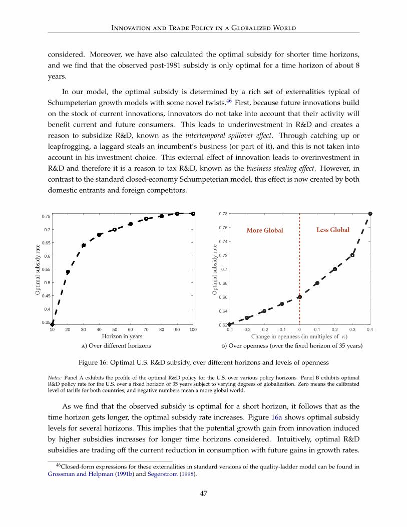
Innovation and Trade Policy in a Globalized World
considered. Moreover, we have also calculated the optimal subsidy for shorter time horizons,and we find that the observed post-1981 subsidy is only optimal for a time horizon of about 8years.
In our model, the optimal subsidy is determined by a rich set of externalities typical ofSchumpeterian growth models with some novel twists.46 First, because future innovations buildon the stock of current innovations, innovators do not take into account that their activity willbenefit current and future consumers. This leads to underinvestment in R&D and creates areason to subsidize R&D, known as the intertemporal spillover effect. Through catching up orleapfrogging, a laggard steals an incumbent’s business (or part of it), and this is not taken intoaccount in his investment choice. This external effect of innovation leads to overinvestment inR&D and therefore it is a reason to tax R&D, known as the business stealing effect. However, incontrast to the standard closed-economy Schumpeterian model, this effect is now created by bothdomestic entrants and foreign competitors.
10 20 30 40 50 60 70 80 90 100
Horizon in years
0.35
0.4
0.45
0.5
0.55
0.6
0.65
0.7
0.75
Opt
imal
sub
sidy
rat
e
a) Over different horizons
-0.4 -0.3 -0.2 -0.1 0 0.1 0.2 0.3 0.4Change in openness (in multiples of )
0.62
0.64
0.66
0.68
0.7
0.72
0.74
0.76
0.78O
ptim
al su
bsid
y ra
te
b) Over openness (over the fixed horizon of 35 years)
Figure 16: Optimal U.S. R&D subsidy, over different horizons and levels of openness
Notes: Panel A exhibits the profile of the optimal R&D policy for the U.S. over various policy horizons. Panel B exhibits optimalR&D policy rate for the U.S. over a fixed horizon of 35 years subject to varying degrees of globalization. Zero means the calibratedlevel of tariffs for both countries, and negative numbers mean a more global world.
As we find that the observed subsidy is optimal for a short horizon, it follows that as thetime horizon gets longer, the optimal subsidy rate increases. Figure 16a shows optimal subsidylevels for several horizons. This implies that the potential growth gain from innovation inducedby higher subsidies increases for longer time horizons considered. Intuitively, optimal R&Dsubsidies are trading off the current reduction in consumption with future gains in growth rates.
46Closed-form expressions for these externalities in standard versions of the quality-ladder model can be found inGrossman and Helpman (1991b) and Segerstrom (1998).
47

Innovation and Trade Policy in a Globalized World
The longer the horizon, the larger the perceived gain from increased growth rate of aggregateconsumption.
Another interesting result is shown in Figure 16b, where we plot the level of optimal subsidyin economies with varying degrees of openness over the same 35-year horizon. It is evident that ina more open economy with smaller iceberg costs, the level of optimal subsidies is lower, implyingthat a less aggressive policy is suitable. This result is again driven by the innovation-boostingeffect of foreign competition through intensification of escape-competition channel.
4.4 Optimal Innovation and Trade Policy
Having analyzed the implications of individual policy options, we now focus on the optimaljoint policy where the U.S. could use both R&D subsidy and one-sided tariff policy in tandem.Figure 17 plots the optimal levels of these policies over different horizons. The left panel showsthat the optimal subsidy levels are close to the ones found when R&D subsidies were consideredin isolation, being only slightly higher in some horizons. The right panel, however, shows thatstrongly protectionist policies are preferred over any horizon, effectively closing the borders toany import penetration. This is in stark contrast with Figure 13a, which shows that optimaltariffs decline with longer horizons, when considered in isolation. The reason is that, beingallowed to set subsidy levels freely, the home country can incentivize its firms to innovate at
10 20 30 40 50 60 70 80 90 100
Horizon in years
0.4
0.45
0.5
0.55
0.6
0.65
0.7
0.75
Opt
imal
R&
D s
ubsi
dy
a) Optimal R&D subsidy
10 20 30 40 50 60 70 80 90 100
Horizon in years
0
0.2
0.4
0.6
0.8
1
1.2
1.4
Opt
imal
tari
ff r
ate
(in
mul
tiple
s of
5)
b) Optimal tariff rate
Figure 17: Optimal joint policy
Notes: The figure illustrates the optimal mix of R&D subsidies and unilateral tariff rates for the U.S. across different policy horizons.Panel A shows the R&D subsidy level in the optimal policy mix for each horizon, and Panel B shows the unilateral tariff level inthe same mix. On the vertical axis, (1 + x) implies x% higher (lower) trade cost relative to the calibrated value for values of x larger(smaller) than zero.
48

Innovation and Trade Policy in a Globalized World
higher rates, compensating for the loss of innovative efforts as a result of lower competitivepressure that protectionism causes. Therefore, allowing the economy to adjust both marginsfreely, the joint policy alternative leads to a highly protectionist regime. However, it is crucialto note that when considering optimal policies, we assumed away any reaction from the foreigncountry and focused only on one-sided tariff policies. Next, we delve into the implications ofsuch a foreign response.
4.5 Effect of Foreign Retaliation on Optimal Policy
Until now, we analyzed the trade policy in a unilateral fashion: The home country could set itstariff rates freely, without facing a response from the foreign country. Although this analysisserves as a helpful benchmark, such unilateral moves would be unlikely in reality. The naturalquestion is, what would be the effect of foreign retaliation on the design of trade policy?47 Toanswer this question, we analyze our policy alternatives under the assumption that any changein tariffs imposed by the home country is perfectly matched by the foreign one. Figure 18 showsthe optimal joint policy in this modified setting with bilateral tariff changes (solid blue lines), injuxtaposition with the results obtained in the benchmark setting (dashed black lines).
10 20 30 40 50 60 70 80 90 100
Horizon in years
0.3
0.35
0.4
0.45
0.5
0.55
0.6
0.65
0.7
0.75
0.8
Opt
imal
R&
D s
ubsi
dy
UnilateralBilateral
a) Optimal R&D subsidy
10 20 30 40 50 60 70 80 90 100
Horizon in years
0.2
0.4
0.6
0.8
1
1.2
1.4
Opt
imal
tari
ff r
ate
(in
mul
tiple
s of
5)
UnilateralBilateral
b) Optimal tariff rate
Figure 18: Optimal joint policy in unilateral and bilateral tariff changes
Notes: The top panel compares horizon-dependent optimal joint policy in case of (trade-policy) retaliation to that in the baseline.Panel A compares R&D subsidies in the optimal mix, while Panel B contrasts trade policies in the optimal mix. On the vertical axis,(1 + x) implies x% higher (lower) trade cost relative to the calibrated value for values of x larger (smaller) than zero.
47The introduction of the Smoot-Hawley Tariff Act in the U.S. during the early stages of the Great Depressionprovides an example of how the unilateral introduction of trade policies could trigger retaliatory responses fromtrade partners, potentially harming the domestic economy.
49
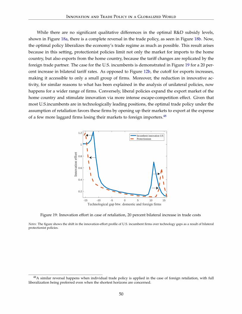
Innovation and Trade Policy in a Globalized World
While there are no significant qualitative differences in the optimal R&D subsidy levels,shown in Figure 18a, there is a complete reversal in the trade policy, as seen in Figure 18b. Now,the optimal policy liberalizes the economy’s trade regime as much as possible. This result arisesbecause in this setting, protectionist policies limit not only the market for imports to the homecountry, but also exports from the home country, because the tariff changes are replicated by theforeign trade partner. The case for the U.S. incumbents is demonstrated in Figure 19 for a 20 per-cent increase in bilateral tariff rates. As opposed to Figure 12b, the cutoff for exports increases,making it accessible to only a small group of firms. Moreover, the reduction in innovative ac-tivity, for similar reasons to what has been explained in the analysis of unilateral policies, nowhappens for a wider range of firms. Conversely, liberal policies expand the export market of thehome country and stimulate innovation via more intense escape-competition effect. Given thatmost U.S.incumbents are in technologically leading positions, the optimal trade policy under theassumption of retaliation favors these firms by opening up their markets to export at the expenseof a few more laggard firms losing their markets to foreign importers.48
-15 -10 -5 0 5 10 15
Technological gap btw. domestic and foreign firms
0.2
0.4
0.6
0.8
1
1.2
Inno
vatio
n ef
fort
Incumbent innovation USProtectionism
Figure 19: Innovation effort in case of retaliation, 20 percent bilateral increase in trade costs
Notes: The figure shows the shift in the innovation-effort profile of U.S. incumbent firms over technology gaps as a result of bilateralprotectionist policies.
48A similar reversal happens when individual trade policy is applied in the case of foreign retaliation, with fullliberalization being preferred even when the shortest horizons are concerned.
50

Innovation and Trade Policy in a Globalized World
5 Sensitivity and Robustness
5.1 Lower maximum technology gap m
Our first exercise considers the robustness of baseline results to the value of the maximum tech-nology gap that can separate two incumbent firms. In our baseline, this value is set to m = 16.As a robustness check, we calculate the empirical gap distribution by setting m = 10 and recali-brate our model accordingly. Figure 20 illustrates the effects of a unilateral increase in U.S. tradebarriers on incumbent firms’ innovation efforts and consumers’ welfare in the U.S. The findingsresonate with Figure 12 both qualitatively and quantitatively, except with a slightly larger wel-fare cost over the long-run. Furthermore, profiles of optimal unilateral policies over differenthorizons, shown in Figure 21, are similar to those found in the baseline calibration. Therefore,we conclude that our original findings are robust to the values of m.
10 20 30 40 50 60 70 80 90 100
Time Periods
-0.8
-0.7
-0.6
-0.5
-0.4
-0.3
-0.2
-0.1
0
0.1
0.2
Perc
enta
ge
Protection
a) Consumption equivalent welfare
-10 -5 0 5 10
Technological gaps btw. domestic and foreign firms
0.1
0.2
0.3
0.4
0.5
0.6
0.7
Inno
vatio
n ef
fort
Incumbent innovation USProtectionism
b) Innovation response to protectionism
Figure 20: Welfare effects of protectionism: unilateral 20 percent increase in trade barriers (m = 10)
Notes: The figure illustrates the effects of a unilateral 20 percent increase in U.S. trade barriers (protectionist U.S. policy withoutretaliatory response). Panel A shows the change in U.S. welfare in consumption equivalent terms over different time horizons. PanelB shows the shift in the innovation-effort profile of U.S. incumbent firms over technology gaps.
5.2 Quality-adjusted gap distribution
In this exercise, we test the robustness of our analysis to the use of citation-weighted patentcounts when forming moments from the data as well as the empirical technology gap distribu-tion. Using citation-weighted patents implies about 4 percent higher share for Japan among allcountries in 1975 at the expense of Germany, the share of which declines by the same amount. As
51

Innovation and Trade Policy in a Globalized World
10 20 30 40 50 60 70 80 90 100
Horizon in years
0.2
0.4
0.6
0.8
1
1.2
1.4
Opt
imal
tari
ff r
ate
(in
mul
tiple
s of
5)
a) Optimal tariff policy over time horizons
10 20 30 40 50 60 70 80 90
Horizon in years
0.35
0.4
0.45
0.5
0.55
0.6
0.65
0.7
0.75
Opt
imal
sub
sidy
rat
e
b) Optimal R&D policy over time horizons
Figure 21: Optimal unilateral policies (m = 10)
Notes: Panel A shows the optimal unilateral tariff policy for the U.S. over various policy horizons. On the vertical axis, (1+ x) impliesx% higher (lower) trade cost relative to the calibrated value for values of x larger (smaller) than zero. Panel B exhibits the profile ofthe optimal R&D policy for the U.S. over various policy horizons.
illustrated in Figure 22a, this reshuffling leads to only minimal changes in the empirical technol-ogy gap distribution, which holds true also for other moments. As a result, the calibration outputis very similar to baseline, as one would expect, when using the alternative measure. Therefore,we skip the rest of the results generated by this alternative calibration.
-20 -15 -10 -5 0 5 10 15 20
Gaps (m)
0
0.01
0.02
0.03
0.04
0.05
0.06
0.07
0.08
0.09
Data US, 1975Data US, 1975, no UK
a) Citation-weighted patents
-20 -15 -10 -5 0 5 10 15 20
Gaps (m)
0
0.01
0.02
0.03
0.04
0.05
0.06
0.07
0.08
0.09
Data US, 1975Data US, 1975, no UK
b) Dropping the U.K.
Figure 22: Alternative initial technological gap distribution
Notes: The figure contrasts alternative initial technological gap distributions (red dashed lines) with the baseline (solid blue lines).Panel A depicts the version omitting the U.K., while panel B shows the version based on citation-weighted patents.
52

Innovation and Trade Policy in a Globalized World
5.3 Dropping the U.K.
As illustrated in Figure 1, the U.K. has a similar productivity and innovation performance tothe U.S. in the late 1970s, in a stark contrast with the other advanced competitors of the U.S.Conjecturing that idiosyncratic factors may have negatively separated the performance of theU.K. from its peers, we recalibrate our model using data that exclude the U.K. For this exercise,we re-weight our targets using data on the remaining five foreign countries, and re-compute theempirical gap distribution. Figure 22b shows that the shift in the initial distribution caused bydropping the U.K. is minuscule, which is also the case with the other targets. Consequently,the parameter values obtained by this alternative calibration, as well as the quantitative results,barely differ from the baseline; hence, we do not repeat them here.
5.4 Lower discount rate ρ
In the baseline calibration, we fixed the discount rate of the households to 1 percent. In orderto test the sensitivity of our results to this parameter, we also ran an alternative calibration,setting the discount rate to 0.5 percent. Our calibration outcome barely changes in this exercisesuggesting that our analysis is robust to varying degrees of the discount rate. Because the effectsare negligible, we skip presenting the results here.
5.5 Excise tariffs
In the baseline exercises, trade policies operate through changes in the level of trade barriers—namely, iceberg costs. In this exercise, we explore the implications of a tariff policy in termsof an excise tax (subsidy) on imports, with the revenue (cost) generated being shared by thehouseholds via lump-sum subsidies (taxes). The profile of the optimal unilateral tariff policy,depicted in Figure 23, mirrors what we found in our baseline setting, although the magnitudeof liberalization, which is again optimal for a far-sighted policy maker, is relatively limited.This result should be expected because in this case, trade liberalization (via import subsidies)comes with an additional cost on households through lump-sum taxes that provide the necessaryfund for subsidies. However, the main message that protectionist policies are only optimal forpolicymakers that have relatively shorter horizons remains intact in this alternative setting.
6 Conclusion
In this paper, we shed light on a recurring debate about the competitiveness of U.S. firms relativeto their foreign competitors and how to improve their position. Motivated by a set of novel facts
53

Innovation and Trade Policy in a Globalized World
10 20 30 40 50 60 70 80 90 100
Horizon in years
0.4
0.5
0.6
0.7
0.8
0.9
1
1.1
1.2
1.3
1.4
Opt
imal
tari
ff r
ate
(in
mul
tiple
s of
5)
Figure 23: Optimal tariff policy with an excise tax
Notes: The figure shows the optimal unilateral tariff policy for the U.S. over various policy horizons. On the vertical axis, (1 + x)means that the U.S. introduces an excise tax on imports of x% of the calibrated trade-cost level. Negative values for x mean a subsidy.
on advanced foreign countries catching up to the U.S. during 1970s and 1980s, we build an openeconomy general equilibrium framework of endogenous growth and trade to evaluate the effec-tiveness of innovation and trade policies in improving the competitiveness of U.S. firms. Firminnovation decisions in our model are motivated by defensive and expansionary innovation mo-tives and domestic and international business-stealing effects. While knowledge spillovers anddecreasing returns to knowledge accumulation lead to cross-country convergence, productivitydifferences drive trade flows. While incorporating an extensive set of realistic relationships, ourmachinery is still well-suited for the analysis of transitional dynamics, which proves to be crucialin policy evaluation.
Our theoretical and quantitative analysis obtains several key results among various others.Theoretically, we show that in the static sense, increased openness benefits the fixed factor inproduction via higher quality intermediate imports raising its compensation, while the impacton business owners is ambiguous, as larger export demand and loss of markets to better foreignrivals exert opposing forces. In the dynamic sense, increased openness, and thus foreign compe-tition, encourages more domestic innovation through an intensified escape-competition channelon defensive and expansionary margins. Quantitatively, we first show that foreign technologicalcatching-up hurts U.S. welfare by stealing away business and profits of U.S. firms. However,over the longer run, the positive dynamic effect of increased foreign competition on domesticinnovation dominates by intensifying the escape-competition effect. Second, we assess that theintroduction of R&D subsidies in the U.S. was a viable response to restore the technological com-petitiveness of U.S. firms, with a notable welfare contribution in the medium term. Moreover,we show that the optimal subsidy is increasing over time horizons and decreasing in openness.
54
Innovation and Trade Policy in a Globalized World
The latter is an intriguing result, which owes again to the positive effect of foreign competitionon domestic innovation through the escape-competition channel. Finally, we consider a counter-factual protectionist response to foreign catching-up. We find that increasing trade barriers forimports unilaterally increases U.S. welfare only in the short run, chiefly through the substitu-tion of imports with domestic production leading to higher domestic profits. However, failingto incentivize U.S. firms to accelerate technological improvement, the protectionist policy can-not compensate for the loss of high quality imports and leads to substantial welfare losses in themedium to long run. Therefore, protectionist policies, despite helping businesses to retain profitsin the short run, make consumers worse off over the longer term.
55

Innovation and Trade Policy in a Globalized World
References
Acemoglu, Daron and Ufuk Akcigit, “Intellectual Property Rights Policy, Competition and In-novation,” Journal of the European Economic Association, 2012, 10 (1), 1–42.
, , Douglas Hanley, and William R. Kerr, “Transition to Clean Technology,” Journal of PoliticalEconomy, 2016, 124 (1), 52–104.
, , Nicholas Bloom, and William R. Kerr, “Innovation, Reallocation and Growth,” 2013.National Bureau of Economic Research Working Paper 18993.
Aghion, Philippe and Peter Howitt, The Economics of Growth, MIT Press, 2009.
, Antonin Bergeaud, Mathieu Lequien, and Marc Melitz, “The Impact of Exports on Innova-tion: Theory and Evidence,” 2017. Manuscript.
, Christopher Harris, and John Vickers, “Competition and Growth with Step-by-step Innova-tion: An Example,” European Economic Review, 1997, 41 (3), 771–782.
, , Peter Howitt, and John Vickers, “Competition, Imitation and Growth with Step-by-stepInnovation,” Review of Economic Studies, 2001, 68 (3), 467–492.
, Nicholas Bloom, Richard Blundell, Rachel Griffith, and Peter Howitt, “Competition andInnovation: An Inverted-U Relationship,” Quarterly Journal of Economics, 2005, 120 (2), 701–728.
Akcigit, Ufuk, Douglas Hanley, and Nicolas Serrano-Velarde, “Back to Basics: Basic ResearchSpillovers, Innovation Policy and Growth,” 2016. Centre for Economic Policy Research Discus-sion Paper 11707.
, , and Stefanie Stantcheva, “Optimal Taxation and R&D Policies,” 2016. National Bureauof Economic Research Working Paper 22908.
Alessandria, George and Horag Choi, “Establishment Heterogeneity, Exporter Dynamics, andthe Effects of Trade Liberalization,” Journal of International Economics, 2014, 94 (2), 207–223.
Antràs, Pol and Elhanan Helpman, “Global Sourcing,” Journal of Political Economy, 2004, 112 (3),552–580.
Arkolakis, Costas, Arnaud Costinot, and Andrés Rodríguez-Clare, “New Trade Models, SameOld Gains?,” American Economic Review, February 2012, 102 (1), 94–130.
Atkeson, Andrew and Ariel T. Burstein, “Innovation, Firm Dynamics, and International Trade,”Journal of Political Economy, 2010, 118 (3), 433–484.
Autor, David, David Dorn, Gordon H. Hanson, Gary Pisano, and Pian Shu, “Foreign Com-petition and Domestic Innovation: Evidence from U.S. Patents,” 2016. National Bureau ofEconomic Research 22879.
Autor, David H., David Dorn, and Gordon H. Hanson, “The China Syndrome: Local LaborMarket Effects of Import Competition in the United States,” American Economic Review, October2013, 103 (6), 2121–2168.
Aw, Bee Yan, Mark J. Roberts, and Daniel Yi Xu, “R&D Investment, Exporting, and ProductivityDynamics,” American Economic Review, 2011, 101 (4), 1312–1344.
56

Innovation and Trade Policy in a Globalized World
Baldwin, Richard and Paul Krugman, “Industrial Policy and International Competition in Wide-bodied Jet Aircraft,” in Richard Baldwin, ed., Trade Policy Issues and Empirical Analysis, Univer-sity of Chicago Press, 1988, pp. 45–78.
Barattieri, Alessandro, Matteo Cacciatore, and Fabio Ghironi, “Protectionism and the BusinessCycle,” 2017. Manuscript.
Bernard, Andrew B., J. Bradford Jensen, Stephen J. Redding, and Peter K. Schott, “GlobalFirms,” Journal of Economic Literature, 2017. forthcoming.
Bloom, Nicholas, Mirko Draca, and John Van Reenen, “Trade Induced Technical Change? TheImpact of Chinese Imports on Innovation, IT and Productivity,” Review of Economic Studies,2016, 83 (1), 87–117.
, Paul M Romer, Stephen J. Terry, and John Van Reenen, “A Trapped-factors Model of Inno-vation,” American Economic Review, Papers and Proceedings, 2013, 103 (3), 208–213.
, Rachel Griffith, and John Van Reenen, “Do R&D Tax Credits Work? Evidence from A Panelof Countries 1979–1997,” Journal of Public Economics, 2002, 85 (1), 1–31.
Buera, Francisco J. and Ezra Oberfield, “The Global Diffusion of Ideas,” 2016. National Bureauof Economic Research 21844.
Burstein, Ariel and Marc J. Melitz, “Trade Liberalization and Firm Dynamics,” in Daron Ace-moglu, Eddie Dekel, and Manuel Arellano, eds., Advances in Economics and Econometrics TenthWorld Congress. Applied Economics, Vol. 2, 2013, pp. 283–328.
Bustos, Paula, “Trade Liberalization, Exports, and Technology Upgrading: Evidence on the Im-pact of MERCOSUR on Argentinian Firms,” American Economic Review, 2011, 101 (1), 304–340.
Cameron, Gavin, James Proudman, and Stephen Redding, “Technological Convergence, R&D,Trade and Productivity Growth,” European Economic Review, 2005, 49 (3), 775–807.
Capdevielle, Patricia and Donato Alvarez, “International Comparisons of Trends in Productivityand Labor Costs,” Monthly Lab. Rev., 1981, 104, 14–20.
Chen, Cheng and Claudia Steinwender, “Import Competition, Heterogeneous Preferences ofManagers, and Productivity,” 2016. Harvard Business School Working Paper.
Coe, David T., Elhanan Helpman, and Alexander W. Hoffmaister, “International R&DSpillovers and Institutions,” European Economic Review, 2009, 53 (7), 723–741.
Coeurdacier, Nicolas and Helene Rey, “Home Bias in Open Economy Financial Macroeco-nomics,” Journal of Economic Literature, 2013, 51 (1), 63–115.
Costinot, Arnaud, Andrés Rodríguez-Clare, and Iván Werning, “Micro to Macro: Optimal TradePolicy with Firm Heterogeneity,” 2016. National Bureau of Economic Research 21989.
, Dave Donaldson, Jonathan Vogel, and Iván Werning, “Comparative Advantage and OptimalTrade Policy,” Quarterly Journal of Economics, 2015, 130 (2), 659–702.
Demidova, Svetlana and Andrés Rodríguez-Clare, “Trade Policy Under Firm-level Heterogene-ity in a Small Economy,” Journal of International Economics, June 2009, 78 (1), 100–112.
57

Innovation and Trade Policy in a Globalized World
Eaton, Jonathan and Gene M. Grossman, “Optimal Trade and Industrial Policy underOligopoly,” Quarterly Journal of Economics, 1986, 101 (2), 383–406.
Gerschenkron, Alexander, Economic Backwards in Historical Perspective: A Book of Essays, BelknapPress of Harvard University Press, 1962.
Grossman, Gene M. and Edwin L.-C. Lai, “International Protection of Intellectual Property,”American Economic Review, 2004, 94 (5), 1635–1653.
and Elhanan Helpman, “Comparative Advantage and Long-run Growth,” American EconomicReview, 1990, 80 (4), 796–815.
and , “Growth and Welfare in a Small Open Economy,” in E. Helpman and A. Razin, eds.,International Trade and Trade Policy, Cambridge, Mass.: MIT Press, 1991, chapter 8, pp. 141–163.
and , “Quality Ladders in the Theory of Growth,” Review of Economic Studies, 1991, 58 (1),43–61.
and , Innovation and Growth In the Global Economy, MIT press, 1993.
Haaland, Jan I. and Hans Jarle Kind, “R&D Policies, Trade and Process Innovation,” Journal ofInternational Economics, 2008, 74 (1), 170–187.
Hall, Bronwyn H., Adam B. Jaffe, and Manuel Trajtenberg, “The NBER Patent Citation DataFile: Lessons, Insights and Methodological Tools,” 2001. National Bureau of Economic Re-search 8498.
Hottman, Colin J., Stephen J. Redding, and David E. Weinstein, “Quantifying the Sources ofFirm Heterogeneity,” Quarterly Journal of Economics, 2016, 131 (3), 1291–1364.
Iacovone, Leonardo, Wolfgang Keller, and Ferdinand Rauch, “Innovation Responses to ImportCompetition,” 2011. Mimeo, Princeton University.
Impullitti, Giammario, “International Competition and US R&D Subsidies: A Quantitative Wel-fare Analysis,” International Economic Review, 2010, 51 (4), 1127–1158.
and Omar Licandro, “Trade, Firm Selection, and Innovation: The Competition Channel,”Economic Journal, 2017.
Irwin, Douglas A. and Nina Pavcnik, “Airbus versus Boeing Revisited: International Competi-tion in the Aircraft Market,” Journal of International Economics, 2004, 64 (2), 223–245.
Keller, Wolfgang, “International Technology Diffusion,” Journal of Economic Literature, 2004, 42(3), 752–782.
Leahy, Dermot and J. Peter Neary, “Public Policy towards R&D in Oligopolistic Industries,”American Economic Review, 1997, 87 (4), 642–662.
Lileeva, Alla and Daniel Trefler, “Improved Access to Foreign Markets Raises Plant-level Pro-ductivity for Some Plants,” Quarterly Journal of Economics, 2010, 125 (3), 1051–1099.
López, Ricardo A., “Do Firms Increase Productivity in Order to Become Exporters?,” OxfordBulletin of Economics and Statistics, 2009, 71 (5), 621–642.
Mayer, Thierry, Marc J. Melitz, and Gianmarco I.P. Ottaviano, “Product Mix and Firm Produc-tivity Responses to Trade Competition,” 2016. National Bureau of Economic Research 22433.
58
Innovation and Trade Policy in a Globalized World
, Marc Melitz, and Gianmarco I.P. Ottaviano, “Market Size, Competition, and the ProductMix of Exporters,” American Economic Review, 2014, 104 (2), 495–536.
Melitz, Marc, “The Impact of Trade on Intra-Industry Reallocations and Aggregate IndustryProductivity,” Econometrica, 2003, 71, 1695–1725.
Melitz, Marc J. and Stephen J. Redding, “Missing Gains from Trade?,” American Economic Re-view, 2014, 104 (5), 317–321.
Muendler, Marc-Andreas, “Trade, Technology, and Productivity: A Study of Brazilian Manufac-turers, 1986-1998,” 2004. CESifo Working Paper Series 1148.
Ossa, Ralph, “A Quantitative Analysis of Subsidy Competition in the US,” 2015. National Bureauof Economic Research Working Paper 20975.
Perla, Jesse, Christopher Tonetti, and Michael E. Waugh, “Equilibrium Technology Diffusion,Trade, and Growth,” 2015. National Bureau of Economic Research Working Paper 20881.
Rivera-Batiz, Luis A. and Paul M. Romer, “Economic Integration and Endogenous Growth,”Quarterly Journal of Economics, 1991, 106 (2), 531–555.
Rodrik, Dani, “Industrial Policy for the Twenty-first Century,” 2004. CEPR Discussion Paper4767.
Romer, Paul M., “Endogenous Technological Change,” Journal of Political Economy, 1990, 98, S71–S102.
Sampson, Thomas, “Dynamic Selection: An Idea Flows Theory of Entry, Trade, and Growth,”Quarterly Journal of Economics, 2016, 131 (1), 315–380.
Segerstrom, Paul S., “Endogenous Growth without Scale Effects,” American Economic Review,1998, 88, 1290–1310.
Spencer, Barbara J. and James A. Brander, “International R&D Rivalry and Industrial Strategy,”Review of Economic Studies, 1983, 50 (4), 707–722.
Wilson, Daniel J., “Beggar Thy Neighbor? The In-state, Out-of-state, and Aggregate Effects ofR&D Tax Credits,” Review of Economics and Statistics, 2009, 91 (2), 431–436.
59

Innovation and Trade Policy in a Globalized World
Appendices
A Additional Empirical Material
A.1 Empirical Facts
This section presents empirical regularities regarding the trends in global technological leader-ship and illustrates technological convergence between the U.S. and other major economies. Adescription of federal- and state-level R&D tax credit policies follows. The section concludes withsuggestive evidence of the effect of R&D tax credits on firm-level performance.
Fact 1: Technological Convergence
There is a striking change in the relative position of foreign countries relative to the U.S. inthe worldwide technological competition over the course of 1970s until mid-80s. Both in theaggregate and sectoral level, we observe a clear pattern of catching-up which we measure usingpatent and citation counts.
.2
.3
.4
.5
Shar
e
1965 1975 1985 1995Application Year
Foreign Share, patents Foreign Share, citations
Figure A.1: Share of foreign patents: 1965-1995
Figure A.1 shows the yearly change in the proportion of patents registered in the U.S. byforeigners using USPTO data on patent counts.49 It also depicts a similar ratio for the citationsthose patents received. Both lines show an obvious, increasing trend, which means that thegrowth in the number of foreign-based patents is higher than the growth in U.S.-based ones.
49The distinction between domestic and foreign patents is by geographic location of registry. For more detail, seeHall et al. (2001).
60

Innovation and Trade Policy in a Globalized World
Interestingly, in the following years the converge process comes to a halt, and we observed aninversion of the trend. Moreover, a glance at the absolute counts, shown in A.2, reveals that thechanges in the shares are chiefly driven by a surge in patent registrations by U.S. residents.
20000
40000
60000
80000
Pate
nts b
y co
untry
1965 1975 1985 1995Application Year
US patents Foreign Patents
a) Patent count
0
100000
200000
300000
400000
500000
Cita
tions
rece
ived
, by
coun
try
1965 1975 1985 1995Application Year
US citations Foreign citations
b) Citation count
Figure A.2: Evolution of R&D credits in the U.S.
Figure A.3 brings the analysis down to the level of patent classes (IPC4) using the same dataset. It delineates the percentage of sectors (broadly defined by patent classes) “owned” by theU.S.- and foreign-based firms over years as well as the percentage of sectors where they are in a“neck-and-neck” position. The ownership of a sector is defined by having more patents than acertain share of patents registered for the particular sector. The situation we call neck-and-neckarises when the difference of the shares of patents held by two countries is less than a threshold,which is 15 percent in this case. This implies that a sector is dominated (owned) by the firms of acountry if their share is above 57.5 percent, and it is neck-and-neck if their share is between 42.5percent and 57.5 percent. The figure shows the declining trend in the percentage of all sectorswhere U.S. firms are dominating until the mid-1980s. This observation demonstrates the relativestrengthening of foreign competitors in the technological competition. Notice that, in line withthe aggregate trends, we observe an inversion of the trend after 1985 also at the sectoral level.50
Fact 2: R&D Tax Incentives
Partly motivated by these and other similar facts, in the late 1970s concerns about the strength ofU.S. industry and its ability to compete in a fast moving global economy increased dramatically.The key issues focused on whether the new technologies arising from federally funded R&Dwere being fully and effectively exploited for the benefit of the national economy, whether therewere barriers slowing down private firms in creating and commercializing innovations and newtechnologies, and whether public-private collaboration in research and innovation could help the
50The results are unchanged when patents are weighted by citations received.
61

Innovation and Trade Policy in a Globalized World
0
0.1
0.2
0.3
0.4
0.5
0.6
0.7
0.8
0.9
1
% o
f IP
C4-
leve
l sec
tors
1975
1975
1975
1985
1985
1985
1995
1995
1995
Lead
Neck&Neck
Follow
Figure A.3: Leadership distribution: share of sectors with U.S. lead, neck-and-neck, foreign lead
U.S. economy in facing these new challenges (NSF, 2016, Tassey, 2007). Several new policy mea-sures were introduced in those years with a particular attention at avoiding unduly substitutionof government for private firms in activities that the latter can naturally perform better. Thesepolicies included several programs to facilitate transfer of the outcome of the federal R&D to pri-vate business (e.g. the National Cooperative Research act in 1984, the Technology Transfer Act,1986), policies strengthening intellectual property rights such as the Bayh-Dole Act (1980), andtax incentives to innovation which started with the Research and Experimentation Tax Credit in1981.
The R&E Tax credit introduced a 25 percent tax deduction on the increase in R&D spendingover the average of the past three years. In 1985 the statutory rate was reduced to 20 percent andin 1990 the base for eligibility was defined as the average of the 1984–1988 R&D to sales ratio(with a maximum of 16 percent) times current sales. The U.S. competitors in high-tech industries,Japan and the large European economies, introduced or had already in place tax incentives forinnovation. Using corporate tax data, Bloom et al. (2002) estimate the R&D subsidy producedby tax policies in the U.S., Japan and key European countries. The data take into account thedifferent tax and tax credit systems used in each country, and measure the reduction in the costof $1 of R&D investment produced by the tax system. Figure 2c shows the R&D tax subsidy forthe set of countries we are interested in.
The variations across countries are mainly due to the presence and effectiveness of a specifictax credit for R&D. The sudden increase in U.S. subsidies, for instance, takes place with theintroduction of the R&E tax credit in 1981 and with the revision of the base defining incrementalR&D in 1990. We can see that in 1980 the reduction in innovation cost attributable to the tax
62
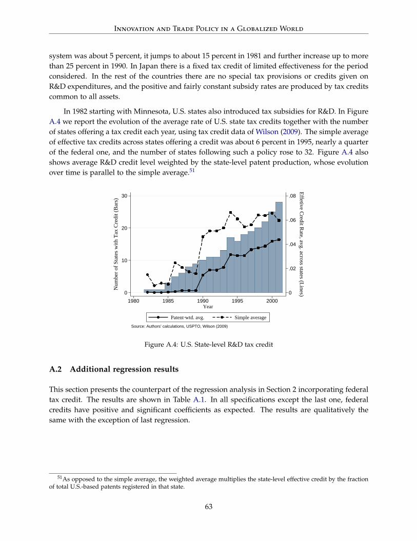
Innovation and Trade Policy in a Globalized World
system was about 5 percent, it jumps to about 15 percent in 1981 and further increase up to morethan 25 percent in 1990. In Japan there is a fixed tax credit of limited effectiveness for the periodconsidered. In the rest of the countries there are no special tax provisions or credits given onR&D expenditures, and the positive and fairly constant subsidy rates are produced by tax creditscommon to all assets.
In 1982 starting with Minnesota, U.S. states also introduced tax subsidies for R&D. In FigureA.4 we report the evolution of the average rate of U.S. state tax credits together with the numberof states offering a tax credit each year, using tax credit data of Wilson (2009). The simple averageof effective tax credits across states offering a credit was about 6 percent in 1995, nearly a quarterof the federal one, and the number of states following such a policy rose to 32. Figure A.4 alsoshows average R&D credit level weighted by the state-level patent production, whose evolutionover time is parallel to the simple average.51
0
.02
.04
.06
.08
Effetive Credit R
ate, avg. across states (Lines)0
10
20
30
Num
ber o
f Sta
tes w
ith T
ax C
redi
t (B
ars)
1980 1985 1990 1995 2000Year
Patent−wtd. avg. Simple average
Source: Authors’ calculations, USPTO, Wilson (2009)
Figure A.4: U.S. State-level R&D tax credit
A.2 Additional regression results
This section presents the counterpart of the regression analysis in Section 2 incorporating federaltax credit. The results are shown in Table A.1. In all specifications except the last one, federalcredits have positive and significant coefficients as expected. The results are qualitatively thesame with the exception of last regression.
51As opposed to the simple average, the weighted average multiplies the state-level effective credit by the fractionof total U.S.-based patents registered in that state.
63

Innovation and Trade Policy in a Globalized World
Table A.1: The Effect of R&D Tax Credit on Innovation (incl. Federal Credits)
Dep. Var.:ln(R&Dt) ln(R&Dt) ln(Patentst) ln(Patentst)
(5) (6) (7) (8)
ln(R&Dt−1)- 0.641 - -- (113.16)∗∗∗ - -
ln(Patentt−1)- - - 0.559- - - (77.22)∗∗∗
ln(State creditt)7.555 0.731 4.255 0.148
(28.72)∗∗∗ (3.26)∗∗ (16.74)∗∗∗ (0.55)
ln(Federal creditt)3.940 1.930 0.563 -0.341
(28.26)∗∗∗ (16.61)∗∗ (4.18)∗∗∗ (-2.41)∗∗
Year Dummy No No No No
Firm Dummy Yes Yes Yes Yes
A.3 Miscellaneous
Figure A.5 replicates Figure 1 over the slightly longer time period 1974-80. The message remainsintact.
Japan
ItalyFrance
Germany
Canada
UKUS
1
2
3
4
5
6
Labo
r Pro
duct
ivity
Gro
wth
in M
anuf
actu
ring
(out
put/h
our,
in %
, 197
4−80
avg
.)
−2 0 2 4 6 8Growth in Patenting
(Patent Applications in the U.S., in %, 1974−80 avg.)
Source: USPTO, Capdevielle and Alvarez (1981), and authors’ own calculation
Figure A.5: Convergence between the U.S. and its peers
64

Innovation and Trade Policy in a Globalized World
B Model and Derivations
B.1 Proofs
Result 1
1. Final Good Price EqualityIntuitively, trade in final good, which is not subject to iceberg costs, equates the final goodprice in both countries (to be 1 as the numeraire). The reason why it is economically viablefor competitive final good producers in both countries to operate, even when there is nofactor price equalitzation for intermediate goods due to trade costs, is that wages adjustaccordingly. Thus, adjustments in the prices of two factors of production guarantee that thefinal good production takes place in both countries at the break even point.To see this consider the profit of the representative final good producer:
Pc (t)Yc(t)−wc(t)Lc−∫ 1
0pj(t)k j(t)dj = Pc (t)Yc(t)−wc(t)Lc−
[∫Ωc
π
βqj(t)dj +
∫Ω∗
π∗
βq∗j (t)dj
].
Here we plugged in intermediate good price from equations (9) and (10). The final goodproducer buys some intermediate goods domestically and and exports some others. Wegroup intermediate goods according to their production location, denoting the measureof domestic and imported intermediate products by Ωc and Ω∗. Referring to the totalexpenditure on domestically bought and imported intermediate goods by ZK
c and MKc ,
respectively, we decompose further:
Pc (t)Yc(t)− wc(t)Lc −∫ 1
0pj(t)k j(t)dj = Pc (t)Yc(t)− wc(t)Lc −
(ZK
c + MKc
)= Pc (t)Yc(t)− βYc(t)− (1− β)Yc(t)
= (Pc (t)− 1)Yc(t).
For the competitive equilibrium in final good production to hold Pc (t) = 1 must hold at alltimes.
2. Trade BalanceWe will show this result in two steps. First, by production approach, GDP equals the sumof value added in final and intermediate good sectors:
GDPc =(
Yc −(
ZKc + MK
c
))+((
ZKc + XK
c
)− Kc
)= Yc − Kc +
(XK
c −MKc
)where Kc is the final good used in intermediate good production, XK
c and MKc represent
the value of exports and imports of intermediate goods, respectively. Then, the national
65

Innovation and Trade Policy in a Globalized World
accounting identity becomes
Yc − Kc +(
XKc −MK
c
)= Cc + Rc + (Xc −Mc)
= Cc + Rc +(
XKc −MK
c
)+(
XYc −MY
c
)where Cc is disposable income/consumption, Dc is investment in R&D, and the (Xc −Mc)
is net exports which we decompose into net exports of intermediate and final goods in thebottom line. Equivalently, the aggregate resource constraint follows as
Yc = Cc + Rc + Kc +(
XYc −MY
c
).
It implies that that the final output in excess of consumption, intermediate input and R&Dexpenditures becomes
(Yc − Dc − Kc)− Cc =(
XYc −MY
c
).
For the second step, denote aggregate sales and profits of domestic firms by Sc and Πc,respectively. We can write total profits as Πc ≡ Sc − Kc =
(ZK
c + XKc)− Kc. Total income
available for consumption is the sum of intermediate firm profits net of R&D expendituresand wages:
Cc = Πc − Dc + βYc.
Substituting this expression for Cc implies that the final output in excess of consumption,intermediate input and R&D expenditures is equal to minus net exports of intermediategoods:
(Yc − Rc − Kc)− Cc = (Yc − Dc − Kc)− (Πc − Dc + βYc)
= (1− β)Yc − (Πc + Kc)
= (1− β)Yc − Sc
=(
ZKc + MK
c
)−(
ZKc + XK
c
)= −
(XK
c −MKc
).
By the equality established previously we obtain
(Yc − Rc − Kc)− Cc =(
XYc −MY
c
)= −
(XK
c −MKc
)⇒(
XYc −MY
c
)+(
XKc −MK
c
)= 0.
66
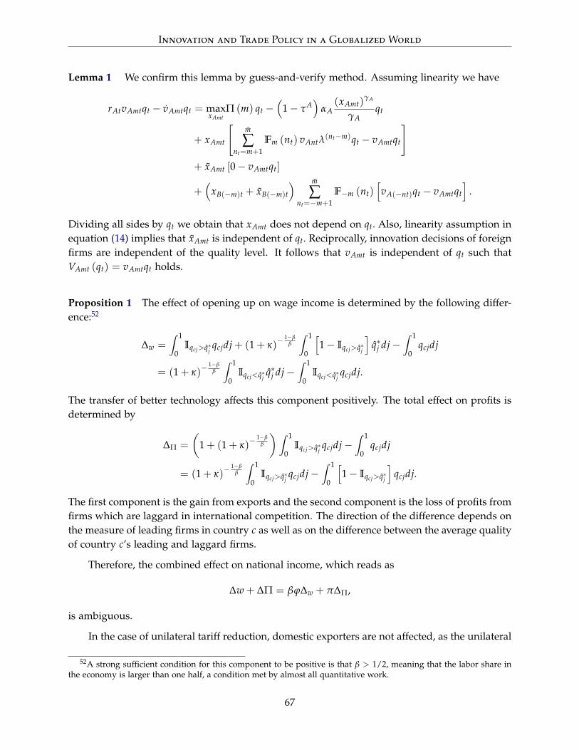
Innovation and Trade Policy in a Globalized World
Lemma 1 We confirm this lemma by guess-and-verify method. Assuming linearity we have
rAtvAmtqt − vAmtqt = maxxAmt
Π (m) qt −(
1− τA)
αA(xAmt)
γA
γAqt
+ xAmt
[m
∑nt=m+1
Fm (nt) vAntλ(nt−m)qt − vAmtqt
]+ xAmt [0− vAmtqt]
+(
xB(−m)t + xB(−m)t
) m
∑nt=−m+1
F−m (nt)[vA(−nt)qt − vAmtqt
].
Dividing all sides by qt we obtain that xAmt does not depend on qt. Also, linearity assumption inequation (14) implies that xAmt is independent of qt. Reciprocally, innovation decisions of foreignfirms are independent of the quality level. It follows that vAmt is independent of qt such thatVAmt (qt) = vAmtqt holds.
Proposition 1 The effect of opening up on wage income is determined by the following differ-ence:52
∆w =∫ 1
0Iqcj>q∗j qcjdj + (1 + κ)
− 1−ββ
∫ 1
0
[1− Iqcj>q∗j
]q∗j dj−
∫ 1
0qcjdj
= (1 + κ)− 1−β
β
∫ 1
0Iqcj<q∗j q∗j dj−
∫ 1
0Iqcj<q∗j qcjdj.
The transfer of better technology affects this component positively. The total effect on profits isdetermined by
∆Π =
(1 + (1 + κ)
− 1−ββ
) ∫ 1
0Iqcj>q∗j qcjdj−
∫ 1
0qcjdj
= (1 + κ)− 1−β
β
∫ 1
0Iqcj>q∗j qcjdj−
∫ 1
0
[1− Iqcj>q∗j
]qcjdj.
The first component is the gain from exports and the second component is the loss of profits fromfirms which are laggard in international competition. The direction of the difference depends onthe measure of leading firms in country c as well as on the difference between the average qualityof country c’s leading and laggard firms.
Therefore, the combined effect on national income, which reads as
∆w + ∆Π = βϕ∆w + π∆Π,
is ambiguous.
In the case of unilateral tariff reduction, domestic exporters are not affected, as the unilateral
52A strong sufficient condition for this component to be positive is that β > 1/2, meaning that the labor share inthe economy is larger than one half, a condition met by almost all quantitative work.
67

Innovation and Trade Policy in a Globalized World
tariff reduction only affects the cutoff for imports. Therefore, its effect is determined by the lossof domestic profits and the gains from technology transfer driven by the higher import volume.
Proposition 2 First, note that v−m = v−m and vm = vm satisfy the set of equation for m > 0.This implies that we have three distinct firm values and innovation rates, and that xm = xm = 0.
Now we show x0 > 0, x−m > 0 and x0 > x−m = x−m.
1. vm > v0 : Assume not such that v0 ≥ vm = v1. Then [v1 − v0] ≤ 0, and x0 = 0. Thisimplies v0 = 0 ≥ vm = v1. But v0 = 0 would mean rvm = 2π − x−mvm and thus vm > 0, acontradiction. Therefore x0 > 0.
2. v0 > v−m: Assume not such that v−m ≥ v0. Then x−m = 0 implying that v−m = 0 ≥ v0.This is possible only if x0 = 0. But since vm > v0 as shown above, x0 > 0, a contradiction.Therefore x−m > 0.
3. [vm − v0] > [v0 − v−m]: Assume not such that [v0 − v−m] ≥ [vm − v0] .This means v0 < 0unless x0 = 0. If v0 < 0, it is a contradiction by step 2. If x0 = 0 meaning that v0 = 0 it isa contradiction by step 1. Therefore [vm − v0] > [v0 − v−m] and x0 > x−m = x−m > xm =
xm = 0.
B.2 Aggregation and the distribution of leadership
The growth rate of this economy is determined by the changes in aggregate quality/productivityacross intermediate goods, Qcmt. In order to analyze the evolution of aggregate quality andbreaking it down into its various sources we need to consider all possible scenarios of inno-vation outcomes and keep track of the resulting changes in quality levels across product linesat each gap size. In the Appendix we describe all possible cases, and here we only report theresulting evolution of aggregate qualities. Changes in QAmt are characterized by the followingexpressions:53
QAmt =m−1
∑s=−m
Fs (m) (xAst + xAst) λm−sQAst +m
∑s=m+1
F−s (−m)(
xB(−s)t + xB(−s)t
)QAst
−[
xAmt + xB(−m)t + xAmt + xB(−m)t
]QAmt
QAmt =[(xAmt + xAmt) (λ− 1)− xB(−m)t − xB(−m)t
]QAmt +
m−1
∑s=−m
Fs (m) (xAst + xAst) λm−sQAst
QA(−m)t =[(xBmt + xBmt) (λ− 1)− xA(−m)t − xA(−m)t
]QA(−m)t +
m−1
∑s=−m
Fs (m) (xBst + xBst) QA(−s)t.
53The evolution of the variables for country B is given reciprocally.
68

Innovation and Trade Policy in a Globalized World
The first equation is the generic expression that describes the change in the aggregate qualityof intermediate goods produced by firms from country c at position m. The first sum capturesthe addition of new incumbents improving to gap m. An innovation with step size λm−s, by adomestic incumbent or entrant at position s < m happens with probability Fs (m), and it impliesthat the domestic incumbent in that product line will reach gap m. The second sum capturesthe addition of product lines, where the position of the domestic incumbent worsened to m froma better one. An improvement by foreign incumbents or entrants from position −s < −m to−m, which happens with probability F−s (−m), hits the domestic incumbent in that productline enjoying the position s > m and brings it down to gap m. The third component in theequation captures the fact that any innovation in a product line where the domestic incumbent isat position m causes a change in its position and thus, a negative change in the aggregate qualityindex across product lines of position m. The other two equations describe the boundary cases.In case of m, notice that innovation by the domestic incumbent or entrants does not change thegap between the domestic incumbent and the foreign follower due to spillover effects, but raisesthe average quality by the step size. Reciprocally, any innovation by the foreign incumbent orentrants improves the quality of the good that the most laggard domestic incumbents producedue to spillover effects.
The laws of motion that determine the measure of product lines where the incumbent fromcountry c is at position m are described by
µAmt = µB(−m)t = ∑m−1s=−m Fs (m) (xAst + xAst) µAst − µAmt
(xB(−m)t + xB(−m)t
)
µAmt = µB(−m)t =
∑ms=m+1 F−s (−m)
(xB(−s)t + xB(−s)t
)µAst
+∑m−1s=−m Fs (m) (xAst + xAst) µAst
−[
xAmt + xB(−m)t + xAmt + xB(−m)t
]µAmt
µA(−m)t = µBmt = ∑m−1s=−m Fs (m) (xBst + xBst) µA(−s)t − µA(−m)t
(xA(−m)t + xA(−m)t
).
(A.1)
The drivers of the dynamics are the same as in the case of aggregate quality indices, exceptthat step sizes are not relevant in determining the levels. Notice that the change in the measure ofposition-m product lines in a country corresponds to the change in the measure of position-(−m)
product lines in the other country. Moreover, because there is a unit measure of intermediateproduct lines we have ∑m µcm = 1. Therefore, information on 2m − 1 measures is enough todescribe the distribution of product lines according to the technological gap size between thetwo active incumbents from each country.
B.3 Derivation of Quality Dynamics
Here we introduce the changes in m in different scenarios and the derivation of Qcmt as re-sult of these changes.Tables below summarize different scenarios (DI (FI): Domestic (Foreign)
69

Innovation and Trade Policy in a Globalized World
Incumbent, DE (FE): Domestic (Foreign) entrant, DN (FN): Domestic (Foreign) competitor inneck-and-neck). The interpretation of a row in the following tables is “in Case X, which happenswith Innov. probability Y, the Effect W is carried into New Position Z”.
The case of m-step-ahead Leader is in country c :
m-step-ahead Leader is in country c
Case Innov. Effect New Position
DI innovates xcm λQc
m m
DE innovates xcm λQc
m m
FI innovates x f−mF−m (n) Qc
m −n
FE innovates x f−mF−m (n) Qc
m −n
Nothing1− xc
m − x f−m
−xcm − x f
−m
Qcm m
The case when m-step-ahead Leader (0 ≤ m < m) is in country c :
m-step-ahead Leader is in country c
Case Innov. Effect New Position
DI innovates xcmFm (n) λ(n−m)Qc
m n
DE innovates xcmFm (n) λ(n−m)Qc
m n
FI innovates x f−mF−m (n) Qc
m −n
FE innovates x f−mF−m (n) Qc
m −n
Nothing1− xc
m − x f−m
−xcm − x f
−m
Qcm m
The case when −m-step-behind Follower (0 < m < m) is in country c :
m-step-behind Follower is in country c
Case Innov. Effect New Position
DI innovates xc−mF−m (n) λ(n+m)Qc
−m n
DE innovates xc−mF−m (n) λ(n+m)Qc
−m n
FI innovates x fmFm (n) Qc
−m −n
FE leapfrogs x fmFm (n) Qc
−m −n
Nothing1− xc
−m − x fm
−xc−m − x f
m
Qc−m −m
70
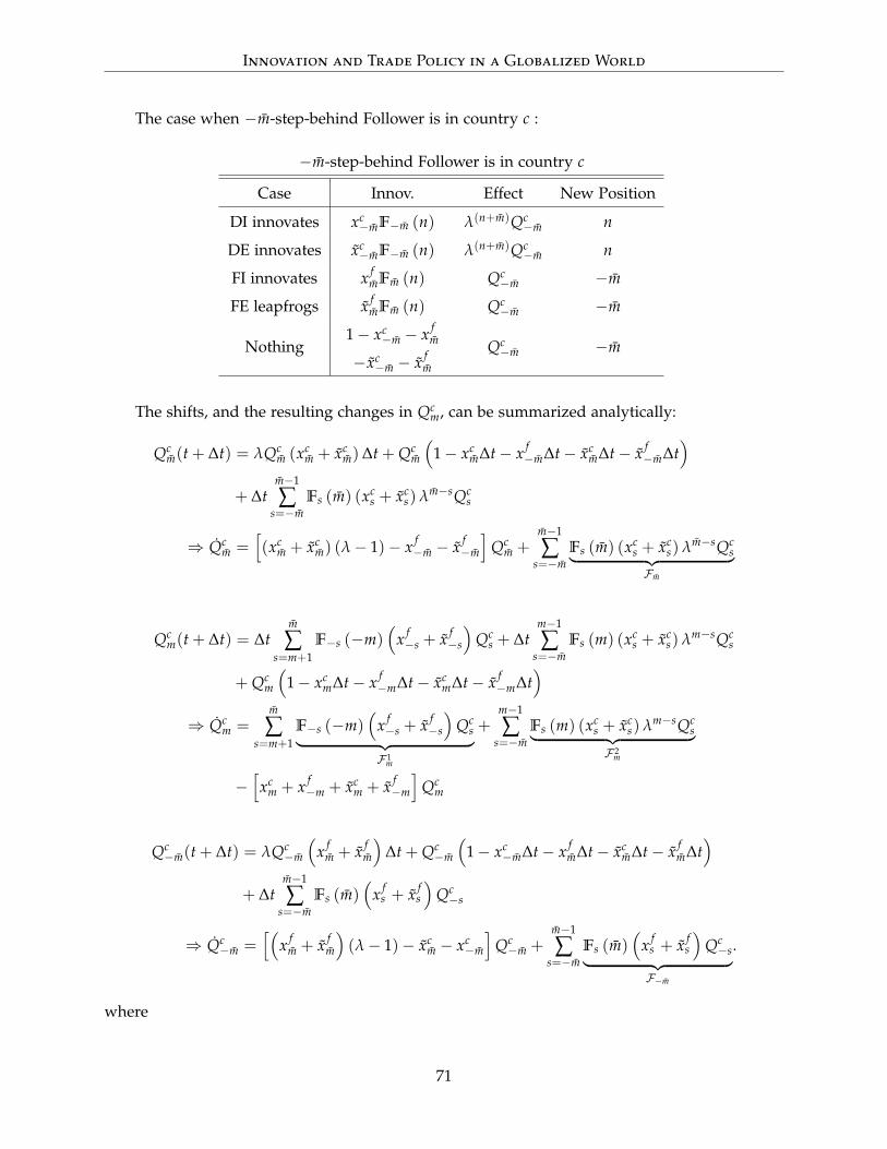
Innovation and Trade Policy in a Globalized World
The case when −m-step-behind Follower is in country c :
−m-step-behind Follower is in country c
Case Innov. Effect New Position
DI innovates xc−mF−m (n) λ(n+m)Qc
−m n
DE innovates xc−mF−m (n) λ(n+m)Qc
−m n
FI innovates x fmFm (n) Qc
−m −m
FE leapfrogs x fmFm (n) Qc
−m −m
Nothing1− xc
−m − x fm
−xc−m − x f
m
Qc−m −m
The shifts, and the resulting changes in Qcm, can be summarized analytically:
Qcm(t + ∆t) = λQc
m (xcm + xc
m)∆t + Qcm
(1− xc
m∆t− x f−m∆t− xc
m∆t− x f−m∆t
)+ ∆t
m−1
∑s=−m
Fs (m) (xcs + xc
s) λm−sQcs
⇒ Qcm =
[(xc
m + xcm) (λ− 1)− x f
−m − x f−m
]Qc
m +m−1
∑s=−m
Fs (m) (xcs + xc
s) λm−sQcs︸ ︷︷ ︸
Fm
Qcm(t + ∆t) = ∆t
m
∑s=m+1
F−s (−m)(
x f−s + x f
−s
)Qc
s + ∆tm−1
∑s=−m
Fs (m) (xcs + xc
s) λm−sQcs
+ Qcm
(1− xc
m∆t− x f−m∆t− xc
m∆t− x f−m∆t
)⇒ Qc
m =m
∑s=m+1
F−s (−m)(
x f−s + x f
−s
)Qc
s︸ ︷︷ ︸F 1
m
+m−1
∑s=−m
Fs (m) (xcs + xc
s) λm−sQcs︸ ︷︷ ︸
F 2m
−[
xcm + x f
−m + xcm + x f
−m
]Qc
m
Qc−m(t + ∆t) = λQc
−m
(x f
m + x fm
)∆t + Qc
−m
(1− xc
−m∆t− x fm∆t− xc
m∆t− x fm∆t
)+ ∆t
m−1
∑s=−m
Fs (m)(
x fs + x f
s
)Qc−s
⇒ Qc−m =
[(x f
m + x fm
)(λ− 1)− xc
m − xc−m
]Qc−m +
m−1
∑s=−m
Fs (m)(
x fs + x f
s
)Qc−s︸ ︷︷ ︸
F−m
.
where
71

Innovation and Trade Policy in a Globalized World
• Fm captures domestic firms at s < m reaching gap m with probability Fs (m) ;
• F 1m captures foreign firms at −s < −m reaching gap −m, thus hitting domestic incumbents
at s > m and bringing them down to gap m, with probability F−s (−m) ;
• F 2m captures domestic firms at s < m reaching gap m with probability Fs (m) ;
• F−m captures foreign firms at s < m reaching gap m, thus hitting domestic incumbents at−s > −m and bringing them down to gap m, with probability Fs (m) .
C Quantitative Appendix
C.1 System in Discrete Time
The discretized system is the system written in terms of instantaneous rate of changes, rightbefore we take the limit as ∆t → 0+ (discarding the terms with (∆t)2). For incumbents andentrants, it is described as follows:
rAt vA
mt+∆t −vA
mt+∆t − vAmt
∆t= Π (m)−
(1− τA
)αA
(xA
mt)γA
γA(A.2)
+ xAmt
m
∑n=m+1
Fm (n) λ(nt−m)vAnt+∆t − vA
mt+∆t
+ xAmt
[0− vA
mt+∆t
]+(
xB−mt + xB
−mt
) m
∑n=−m+1
F−m (n)[vA−nt+∆t − vA
mt+∆t
]
vcmt = −αc
γc(xc
mt)γc + xc
mt
m
∑n=m+1
Fm (n) λ(nt−m)vAnt+∆t − 0
. (A.3)
C.2 Solution Algorithm
1. Let M be the set of data moments and Mm be the model counterpart. Define R (M−Mm)
as the function that calculates a weighted sum of the difference between data and modelmoments.
2. Guess a set of values for the internally calibrated parameters θguess.
3. Calculate the steady state, where time derivatives are zero by definition. Start iterationh = 0 with the guess
rA
T , rBTh=0 .
(a) At iteration h, take
rAT , rB
Th given and solve incumbent firm values jointly for both
countries by backward iteration.
72

Innovation and Trade Policy in a Globalized World
i. Guess
vAmT+∆t, vB
mT+∆t
m∈−m,..,m. Assuming these to be true steady state values
compute innovation rates
xAmT, xA
mT, xBmT, xB
mT
m∈−m,..,m. Notice that these areinnovation rates at one period before as innovation is a forward looking decisionand thus, depends on next period value in discrete time.
ii. Compute
vAmT, vB
mT
m using the value function equations. By the definition of thesteady state, values at T + ∆t and T should be the same.
iii. Check ifmax
m,c
∥∥vcmT+∆t − vc
mT∥∥ < ε.
If not met, set
vcmT+∆t
m = vc
mTm and repeat.
(b) Take the steady state innovation rates, and set QAm0 = 1 ∀m. Iterate forward onaggregate quality indices Qcmt using the transition equations until growth rates of theimplied income processes for both countries stabilize. Call these
gA
T , gBTh .
(c) Check if
rAT , rB
Th and
gA
T , gBTh meet the Euler equation. If not, set
rA
T , rBTh+1 to
interest rates implied by the Euler equation with
gAT , gB
Th and repeat until conver-
gence.
4. Next calculate the equilibrium over the transition. Start iteration h = 0 by guessing a timepath for interest rates
rA
t , rBth=0
t=1975,...,1975+T . The terminal values are set to steady state atevery iteration.
(a) At iteration h, given terminal (steady state) values
vAmT, vB
mTh
m compute the
implied innovation rates
xAmT−∆t, xA
mT−∆t, xBmT−∆t, xB
mT−∆th
m . Then, given termi-
nal interest rates
rAT , rB
Th, compute
vA
mT−∆t, vBmT−∆t
hm . Iterate backwards us-
ing the
rAt , rB
th
t=1975,...,1975+T until t0 = 1975 to obtain the implied seriesxA
mt, xAmt, xB
mt, xBmth
mt=1975,...,1975+T .
(b) Set QAm0 = 1 ∀m. Using the implied innovation rates, compute Qcmt for t =
1975, ..., 1975 + T by forward iteration and back up the implied income processes.
(c) Compute income growth rates
gAt , gB
th
t . Using period-by-period Euler equations,check if
maxm,c,t
∥∥∥∥∥gcth − r
cth − ρ
ψ
∥∥∥∥∥ < ε.
for 1975, ..., 1975 + T − 1. If not, set
rAt , rB
th+1
t=1975,...,1975+T−1 to interest rates im-
plied by the Euler equation with
gAt , gB
th
t=1975,...,1975+T−1 and repeat until conver-gence.
5. Once step 4 converges, use the final interest rates
rAt , rB
t
t=1975,...,1975+T to compute theaggregate variables and the model counterparts of the data moments.
6. Minimize R(M−Mm (θguess
))using an optimization routine.
73

Innovation and Trade Policy in a Globalized World
C.3 Additional Figures
-15 -10 -5 0 5 10 15
Gaps (m)
0.2
0.4
0.6
0.8
1
1.2
Inno
vatio
n ef
fort
Incumbent innovation USR&D subsidy
a) Incumbents
-15 -10 -5 0 5 10 15
Gaps (m)
0.085
0.09
0.095
0.1
0.105
0.11
0.115
Pois
son
arri
val r
ate
Entrant innovation USR&D subsidy
b) Entrants
Figure A.6: Changes in R&D decisions after subsidy change
1985 1990 1995 2000 2005
Years
1
1.5
2
2.5
3
3.5
Mea
n te
chno
logy
gap
of
U.S
. fir
ms
No interventionProtectionism
a) 20 percent tariff hike
1985 1990 1995 2000 2005
Years
1
1.5
2
2.5
3
3.5
Mea
n te
chno
logy
gap
of
U.S
. fir
ms
No interventionHigher subsidy
b) Actual R&D policy
Figure A.7: Average technology lead of the U.S. firms, after policy intervention
74

Innovation and Trade Policy in a Globalized World
12
34
56
Pate
nt a
pplic
atio
n pe
r firm
, avg
.
−15 −10 −5 0 5 10 15Gaps
Figure A.8: Patenting intensity in USPTO data
D Robustness
D.1 Modeling Labor in the Intermediate Goods Sector
A central concern in the debate on gains from trade is the potential harm that import penetrationcan cause to domestic workers by stealing the market of the domestic firms [Autor et al. (2013)].In our baseline model, labor, which is used in the final good sector, benefits from trade liberal-ization thanks to the higher labor productivity, which is brought about by better-quality importsreplacing inferior domestic counterparts. In this section, we modify the baseline model in orderto allow trade to have an adverse impact on labor. In this version, labor is utilized in the pro-duction of intermediate goods; therefore, foreign catch-up leads to a wage loss as a by-productof business stealing. We re-estimate this new version of the model, and compare its key policyimplications with the ones of the baseline model.
Assume that final goods are produced by combining a fixed factor (again normalized to 1for both countries), while intermediate goods are produced using labor:
k jt =qct
ηljt.
Here, qct denotes the economy-wide labor productivity in intermediate good production, whichis common across all sectors. Equilibrium profits from domestic sales and exports become
π(qjt)=
[1− β
η
qct
wct
] 1−ββ
βqjt and π∗(qjt)=
[1− β
(1 + κ) η
qct
wct
] 1−ββ
βL f qcjt.
Market clearing condition for labor reads as Lc =∫ 1
0 lcjt dj. Normalizing the size of the labor
75

Innovation and Trade Policy in a Globalized World
force to 1 and solving for the wage yields
wct
qct= χq−β
ct
QDct + QX
ct + (1 + κ)β−1
β QXct︸ ︷︷ ︸
denote Qct
β
≡ χ
[Qct
qct
]β
.
Here, Qct can be interpreted as the average quality of sales of all active domestic firms, adjustedfor trade costs exported goods are subject to. In the special case where qct = Qct we have
wct = χQct.
Therefore, χQct replaces the term wctLct in the aggregate consumption defined in equation (16):
Cct =m
∑s=m∗
π∗F∗Qcst +m
∑s=−m∗+1
πFcQcst −−m
∑s=−m
αcxγccstQcst −
−m
∑s=−m
αc xγccstQcst
+ βm
∑m=−m∗+1
[1− β
η
] 1−ββ Qcmt
1− β+ β
−m∗
∑m=−m
[1− β
(1 + κ) η
] 1−ββ Q∗mt
1− β+ χQct (A.4)
where Fc, F∗ denote the fixed factor used in the final good production in home and foreigncountries, respectively.
D.1.1 Calibration
We recalibrate this model following similar steps as with the baseline version. This time we setβ to 0.2, allowing us to get a reasonable share of labor income around 65 percent. The rest ofthe external parameters share the baseline values. Internally calibrated parameters are presentedin Table A.2. As summarized in Table A.3, this model also performs well in matching the datatargets.
Table A.2: Internally Calibrated Parameters
R&D scale R&D scale Step size Iceberg F (n)
αA αB αA αB λ κ φ
0.16 0.69 21.0 31.2 0.82% 2.69% 0.77
76
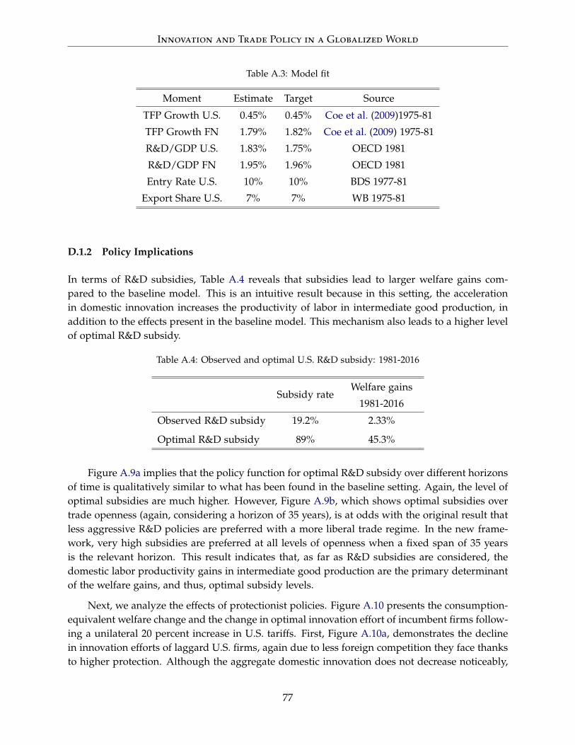
Innovation and Trade Policy in a Globalized World
Table A.3: Model fit
Moment Estimate Target Source
TFP Growth U.S. 0.45% 0.45% Coe et al. (2009)1975-81
TFP Growth FN 1.79% 1.82% Coe et al. (2009) 1975-81
R&D/GDP U.S. 1.83% 1.75% OECD 1981
R&D/GDP FN 1.95% 1.96% OECD 1981
Entry Rate U.S. 10% 10% BDS 1977-81
Export Share U.S. 7% 7% WB 1975-81
D.1.2 Policy Implications
In terms of R&D subsidies, Table A.4 reveals that subsidies lead to larger welfare gains com-pared to the baseline model. This is an intuitive result because in this setting, the accelerationin domestic innovation increases the productivity of labor in intermediate good production, inaddition to the effects present in the baseline model. This mechanism also leads to a higher levelof optimal R&D subsidy.
Table A.4: Observed and optimal U.S. R&D subsidy: 1981-2016
Subsidy rateWelfare gains
1981-2016
Observed R&D subsidy 19.2% 2.33%
Optimal R&D subsidy 89% 45.3%
Figure A.9a implies that the policy function for optimal R&D subsidy over different horizonsof time is qualitatively similar to what has been found in the baseline setting. Again, the level ofoptimal subsidies are much higher. However, Figure A.9b, which shows optimal subsidies overtrade openness (again, considering a horizon of 35 years), is at odds with the original result thatless aggressive R&D policies are preferred with a more liberal trade regime. In the new frame-work, very high subsidies are preferred at all levels of openness when a fixed span of 35 yearsis the relevant horizon. This result indicates that, as far as R&D subsidies are considered, thedomestic labor productivity gains in intermediate good production are the primary determinantof the welfare gains, and thus, optimal subsidy levels.
Next, we analyze the effects of protectionist policies. Figure A.10 presents the consumption-equivalent welfare change and the change in optimal innovation effort of incumbent firms follow-ing a unilateral 20 percent increase in U.S. tariffs. First, Figure A.10a, demonstrates the declinein innovation efforts of laggard U.S. firms, again due to less foreign competition they face thanksto higher protection. Although the aggregate domestic innovation does not decrease noticeably,
77

Innovation and Trade Policy in a Globalized World
10 20 30 40 50 60 70 80 90 100
Horizon in years
0.84
0.85
0.86
0.87
0.88
0.89
0.9
Opt
imal
sub
sidy
rat
e
a) Over different horizons
-0.4 -0.3 -0.2 -0.1 0 0.1 0.2 0.3 0.4
Change in openness (in multiples of 5)
0.76
0.78
0.8
0.82
0.84
0.86
0.88
0.9
Opt
imal
sub
sidy
rat
e
b) Over openness (over the fixed horizon of 35 years)
Figure A.9: Optimal U.S. R&D subsidy, over different horizons and levels of openness
as shown in Figure A.11a, the steady level of innovation cannot compensate for the loss of fore-gone technology of imported goods, and therefore, leads to a declining trend in welfare gainsover longer time periods.54 However, in sharp contrast with the baseline, the protectionist policyleads to welfare gains over all time horizons in this modified setting. The reason is that now pro-tectionist policies prohibit not only business stealing, but also “wage stealing”, i.e. the decline inwages because of the loss of domestic activity to foreign importers. This mechanism strengthensthe positive effect of protectionist policies.
-15 -10 -5 0 5 10 15
Gaps (m)
0.2
0.4
0.6
0.8
1
1.2
1.4
1.6
1.8
Inno
vatio
n ef
fort
Incumbent innovation USProtectionism
a) Consumption equivalent welfare
10 20 30 40 50 60 70 80 90 100
Time Periods
0.3
0.35
0.4
0.45
0.5
0.55
0.6
Perc
enta
ge
Protection
b) Innovation response of incumbents
Figure A.10: Welfare effects of protectionism: unilateral 20 percent increase in trade barriers
54Aggregate incumbent innovation is little affected by the changes in innovation efforts fo individual firms as aresult of protectionist policies because of the limited mass of firms affected.
78

Innovation and Trade Policy in a Globalized World
Turning to optimal unilateral tariffs over different time horizons, shown in Figure A.11b, weobserve that over any time horizon, a high enough tariff rate is preferred such that the economycloses its borders to any import penetration. This boundary result is again very different than itsbaseline counterpart of a declining optimal tariff policy over longer time horizons. Again, this isan intuitive result given that protectionist policies protect domestic wage income in this setting.Moreover, as opposed to the baseline model, the impact of protectionist policies on innovation ismuted in this setting, although we observe the negative effect on individual firms due to weakercompetition. This result arises because of the transitional dynamics of mass of firms affected bythe policy.55
0.5 0.6 0.7 0.8 0.9 1 1.1 1.2 1.3
Tariff rate (in multiples of 5)
0.1
0.15
0.2
0.25
0.3
0.35
0.4
Ave
rage
inno
vatio
n in
tens
ity
IncumbentEntrant
a) Optimal innovation response to tariffs
10 20 30 40 50 60 70 80 90 100
Horizon in years
0.6
0.8
1
1.2
1.35
Opt
imal
tari
ff r
ate
(in
mul
tiple
s of
5)
b) Optimal tariff policy
Figure A.11: Innovation response to tariffs and optimal tariff rate
Finally, Figure A.12 shows the optimal joint policy response, both in cases of unilateral(dashed black lines) and bilateral (solid blue lines) tariff changes. In the former setting, optimallevels of individual policies closely follow their counterparts obtained when policy alternativesare considered in isolation. Furthermore, as in the baseline model, the reversal in the trade policywhen the foreign country retaliates arises also in this modified model. This result implies thatthe gains from wider export markets for the home firms dominate the additional negative effectof import penetration on domestic wages.
55These dynamics limit the fall in welfare gains over time in Figure A.10b.
79

Innovation and Trade Policy in a Globalized World
10 20 30 40 50 60 70 80 90 100
Horizon in years
0.8
0.82
0.84
0.86
0.88
0.9
0.92
0.94
Opt
imal
R&
D s
ubsi
dy
UnilateralBilateral
a) Optimal R&D subsidy
10 20 30 40 50 60 70 80 90 100
Horizon in years
0.2
0.4
0.6
0.8
1
1.2
Opt
imal
tari
ff r
ate
(in
mul
tiple
s of
5)
UnilateralBilateral
b) Optimal tariff rate
Figure A.12: Optimal joint policy
80