Inorganic Chemistry

This page intentionally left blank

Inorganic Chemistry

James E. House

Illinois Wesleyan University and Illinois State University

AMSTERDAM • BOSTON • HEIDELBERG • LONDON • OXFORD • NEW YORKPARIS • SAN DIEGO • SAN FRANCISCO • SINGAPORE • SYDNEY • TOKYO

Academic Press is an imprint of Elsevier

Academic Press is an imprint of Elsevier 30 Corporate Drive, Suite 400, Burlington, MA 01803, USA 525 B Street, Suite 1900, San Diego, California 92101-4495, USA 84 Theobald’s Road, London WC1X 8RR, UK

� This book is printed on acid-free paper.

Copyright © 2008, Elsevier Inc. All rights reserved.

No part of this publication may be reproduced or transmitted in any form or by any means, electronic or mechanical, including photocopy, recording, or any information storage and retrieval system, without permission in writing from the publisher.

Permissions may be sought directly from Elsevier’s Science & Technology Rights Department in Oxford, UK: phone: ( � 44) 1865 843830, fax: ( � 44) 1865 853333, E-mail: permissions@elsevier.com. You may also complete your request on-line via the Elsevier homepage ( http://elsevier.com ), by selecting “ Support & Contact ” then “ Copyright and Permission ” and then “ Obtaining Permissions. ”

Library of Congress Cataloging-in-Publication Data

House, J. E. Inorganic chemistry / James E. House. p. cm. Includes index. ISBN 978-0-12-356786-4 (paper cover : alk. paper) 1. Chemistry, Inorganic—Textbooks. I. Title.

QD151.5.H68 2008 546—dc22 2008013083

British Library Cataloguing-in-Publication Data A catalogue record for this book is available from the British Library.

ISBN: 978-0-12-356786-4

For information on all Academic Press publications visit our Web site at www.books.elsevier.com

Printed in Canada

08 09 10 11 9 8 7 6 5 4 3 2 1

Contents

Preface xi

PART 1 Structure of Atoms and Molecules 1

CHAPTER 1 Light, Electrons, and Nuclei 3

1.1 Some Early Experiments in Atomic Physics 3 1.2 The Nature of Light 7 1.3 The Bohr Model 11 1.4 Particle-Wave Duality 15 1.5 Electronic Properties of Atoms 17 1.6 Nuclear Binding Energy 22 1.7 Nuclear Stability 24 1.8 Types of Nuclear Decay 25 1.9 Predicting Decay Modes 29

CHAPTER 2 Basic Quantum Mechanics and Atomic Structure 35

2.1 The Postulates 35 2.2 The Hydrogen Atom 44 2.3 The Helium Atom 49 2.4 Slater Wave Functions 51 2.5 Electron Confi gurations 52 2.6 Spectroscopic States 56

CHAPTER 3 Covalent Bonding in Diatomic Molecules 65

3.1 The Basic Ideas of Molecular Orbital Methods 65 3.2 The H 2 � and H 2 Molecules 73 3.3 Diatomic Molecules of Second-Row Elements 76 3.4 Photoelectron Spectroscopy 83 3.5 Heteronuclear Diatomic Molecules 84 3.6 Electronegativity 87 3.7 Spectroscopic States for Molecules 91

CHAPTER 4 A Survey of Inorganic Structures and Bonding 95

4.1 Structures of Molecules Having Single Bonds 95 4.2 Resonance and Formal Charge 105

4.3 Complex Structures—A Preview of Coming Attractions 117 4.4 Electron-Defi cient Molecules 125 4.5 Structures Having Unsaturated Rings 127 4.6 Bond Energies 129

CHAPTER 5 Symmetry and Molecular Orbitals 137

5.1 Symmetry Elements 137 5.2 Orbital Symmetry 145 5.3 A Brief Look at Group Theory 148 5.4 Construction of Molecular Orbitals 153 5.5 Orbitals and Angles 158 5.6 Simple Calculations Using the Hückel Method 161

PART 2 Condensed Phases 177

CHAPTER 6 Dipole Moments and Intermolecular Interactions 179

6.1 Dipole Moments 179 6.2 Dipole-Dipole Forces 184 6.3 Dipole-Induced Dipole Forces 186 6.4 London (Dispersion) Forces 187 6.5 The van der Waals Equation 191 6.6 Hydrogen Bonding 193 6.7 Cohesion Energy and Solubility Parameters 203

CHAPTER 7 Ionic Bonding and Structures of Solids 211

7.1 Energetics of Crystal Formation 211 7.2 Madelung Constants 216 7.3 The Kapustinskii Equation 219 7.4 Ionic Sizes and Crystal Environments 220 7.5 Crystal Structures 224 7.6 Solubility of Ionic Compounds 229 7.7 Proton and Electron Affi nities 234 7.8 Structures of Metals 237 7.9 Defects in Crystals 240 7.10 Phase Transitions in Solids 243 7.11 Heat Capacity 245 7.12 Hardness of Solids 248

CHAPTER 8 Dynamic Processes in Inorganic Solids 255

8.1 Characteristics of Solid-State Reactions 255 8.2 Kinetic Models for Reactions in Solids 258

vi Contents

8.3 Thermal Methods of Analysis 266 8.4 Effects of Pressure 267 8.5 Reactions in Some Solid Inorganic Compounds 270 8.6 Phase Transitions 272 8.7 Reactions at Interfaces 276 8.8 Diffusion in Solids 277 8.9 Sintering 280 8.10 Drift and Conductivity 282

PART 3 Acids, Bases, and Solvents 287

CHAPTER 9 Acid-Base Chemistry 289

9.1 Arrhenius Theory 289 9.2 Brønsted-Lowry Theory 292 9.3 Factors Affecting Strength of Acids and Bases 296 9.4 Acid-Base Character of Oxides 301 9.5 Proton Affi nities 302 9.6 Lewis Theory 305 9.7 Catalytic Behavior of Acids and Bases 309 9.8 The Hard-Soft Interaction Principle (HSIP) 313 9.9 Electronic Polarizabilities 323 9.10 The Drago Four-Parameter Equation 324

CHAPTER 10 Chemistry in Nonaqueous Solvents 331

10.1 Some Common Nonaqueous Solvents 331 10.2 The Solvent Concept 332 10.3 Amphoteric Behavior 335 10.4 The Coordination Model 335 10.5 Chemistry in Liquid Ammonia 336 10.6 Liquid Hydrogen Fluoride 342 10.7 Liquid Sulfur Dioxide 345 10.8 Superacids 349

PART 4 Chemistry of the Elements 353

CHAPTER 11 Chemistry of Metallic Elements 355

11.1 The Metallic Elements 355 11.2 Band Theory 356 11.3 Group IA and IIA Metals 359 11.4 Zintl Phases 367 11.5 Aluminum and Beryllium 370

Contents vii

11.6 The First-Row Transition Metals 372 11.7 Second- and Third-Row Transition Metals 374 11.8 Alloys 376 11.9 Chemistry of Transition Metals 379 11.10 The Lanthanides 387

CHAPTER 12 Organometallic Compounds of the Main Group Elements 395

12.1 Preparation of Organometallic Compounds 396 12.2 Organometallic Compounds of Group IA Metals 398 12.3 Organometallic Compounds of Group IIA Metals 400 12.4 Organometallic Compounds of Group IIIA Metals 403 12.5 Organometallic Compounds of Group IVA Metals 408 12.6 Organometallic Compounds of Group VA Elements 409 12.7 Organometallic Compounds of Zn, Cd, and Hg 410

CHAPTER 13 Chemistry of Nonmetallic Elements I. Hydrogen, Boron, Oxygen and Carbon 415

13.1 Hydrogen 415 13.2 Boron 422 13.3 Oxygen 433 13.4 Carbon 444

CHAPTER 14 Chemistry of Nonmetallic Elements II. Groups IVA and VA 463

14.1 The Group IVA Elements 463 14.2 Nitrogen 480 14.3 Phosphorus, Arsenic, Antimony, and Bismuth 497

CHAPTER 15 Chemistry of Nonmetallic Elements III. Groups VIA to VIIIA 523

15.1 Sulfur, Selenium, and Tellurium 523 15.2 The Halogens 545 15.3 The Noble Gases 564

PART 5 Chemistry of Coordination Compounds 575

CHAPTER 16 Introduction to Coordination Chemistry 577

16.1 Structures of Coordination Compounds 577 16.2 Metal-Ligand Bonds 582 16.3 Naming Coordination Compounds 583 16.4 Isomerism 585 16.5 A Simple Valence Bond Description of Coordinate Bonds 592 16.6 Magnetism 597 16.7 A Survey of Complexes of First-Row Metals 599

viii Contents

16.8 Complexes of Second- and Third-Row Metals 599 16.9 The 18-Electron Rule 601 16.10 Back Donation 604 16.11 Complexes of Dinitrogen, Dioxygen, and Dihydrogen 609

CHAPTER 17 Ligand Fields and Molecular Orbitals 617

17.1 Splitting of d Orbital Energies in Octahedral Fields 617 17.2 Splitting of d Orbital Energies in Fields of Other Symmetry 621 17.3 Factors Affecting Δ 625 17.4 Consequences of Crystal Field Splitting 627 17.5 Jahn-Teller Distortion 630 17.6 Spectral Bands 631 17.7 Molecular Orbitals in Complexes 633

CHAPTER 18 Interpretation of Spectra 645

18.1 Splitting of Spectroscopic States 645 18.2 Orgel Diagrams 650 18.3 Racah Parameters and Quantitative Methods 652 18.4 The Nephelauxetic Effect 655 18.5 Tanabe-Sugano Diagrams 658 18.6 The Lever Method 662 18.7 Jørgensen’s Method 665 18.8 Charge Transfer Absorption 666

CHAPTER 19 Composition and Stability of Complexes 671

19.1 Composition of Complexes in Solution 671 19.2 Job’s Method of Continuous Variations 673 19.3 Equilibria Involving Complexes 675 19.4 Distribution Diagrams 681 19.5 Factors Affecting the Stability of Complexes 685

CHAPTER 20 Synthesis and Reactions of Coordination Compounds 695

20.1 Synthesis of Coordination Compounds 695 20.2 Substitution Reactions in Octahedral Complexes 701 20.3 Ligand Field Effects 708 20.4 Acid-Catalyzed Reactions of Complexes 712 20.5 Base-Catalyzed Reactions of Complexes 713 20.6 The Compensation Effect 715 20.7 Linkage Isomerization 716 20.8 Substitution in Square Planar Complexes 719 20.9 The Trans Effect 721

Contents ix

20.10 Electron Transfer Reactions 725 20.11 Reactions in Solid Coordination Compounds 728

CHAPTER 21 Complexes Containing Metal-Carbon and Metal-Metal Bonds 739

21.1 Binary Metal Carbonyls 739 21.2 Structures of Metal Carbonyls 742 21.3 Bonding of Carbon Monoxide to Metals 744 21.4 Preparation of Metal Carbonyls 747 21.5 Reactions of Metal Carbonyls 748 21.6 Structure and Bonding in Metal Alkene Complexes 754 21.7 Preparation of Metal Alkene Complexes 760 21.8 Chemistry of Cyclopentadienyl and Related Complexes 761 21.9 Bonding in Ferrocene 764 21.10 Reactions of Ferrocene and Other Metallocenes 767 21.11 Complexes of Benzene and Related Aromatics 770 21.12 Compounds Containing Metal-Metal Bonds 773

CHAPTER 22 Coordination Compounds in Catalysis and Biochemistry 779

22.1 Elementary Steps in Catalysis Processes 780 22.2 Homogeneous Catalysis 792 22.3 Bioinorganic Chemistry 802

Appendix A: Ionization Energies 817

Appendix B: Character Tables for Selected Point Groups 821

Index 827

x Contents

No single volume, certainly not a textbook, can come close to including all of the important topics in inorganic chemistry. The fi eld is simply too broad in scope and it is growing at a rapid pace. Inorganic chemistry textbooks refl ect a great deal of work and the results of the many choices that authors must make as to what to include and what to leave out. Writers of textbooks in chemistry bring to the task backgrounds that refl ect their research interests, the schools they attended, and their personalities. In their writing, authors are really saying “this is the fi eld as I see it.“ In these regards, this book is similar to others.

When teaching a course in inorganic chemistry, certain core topics are almost universally included. In addition, there are numerous peripheral areas that may be included at certain schools but not at oth-ers depending on the interests and specialization of the person teaching the course. The course content may even change from one semester to the next. The effort to produce a textbook that presents cover-age of a wide range of optional material in addition to the essential topics can result in a textbook for a one semester course that contains a thousand pages. Even a “concise” inorganic chemistry book can be nearly this long. This book is not a survey of the literature or a research monograph. It is a text-book that is intended to provide the background necessary for the reader to move on to those more advanced resources.

In writing this book, I have attempted to produce a concise textbook that meets several objectives. First, the topics included were selected in order to provide essential information in the major areas of inor-ganic chemistry (molecular structure, acid-base chemistry, coordination chemistry, ligand fi eld theory, solid state chemistry, etc.). These topics form the basis for competency in inorganic chemistry at a level commensurate with the one semester course taught at most colleges and universities.

When painting a wall, better coverage is assured when the roller passes over the same area several times from different directions. It is the opinion of the author that this technique works well in teaching chemistry. Therefore, a second objective has been to stress fundamental principles in the discussion of several topics. For example, the hard-soft interaction principle is employed in discussion of acid-base chemistry, stability of complexes, solubility, and predicting reaction products. Third, the presentation of topics is made with an effort to be clear and concise so that the book is portable and user friendly. This book is meant to present in convenient form a readable account of the essentials of inorganic chemistry that can serve as both as a textbook for a one semester course upper level course and as a guide for self study. It is a textbook not a review of the literature or a research monograph. There are few references to the original literature, but many of the advanced books and monographs are cited.

Although the material contained in this book is arranged in a progressive way, there is fl exibility in the order of presentation. For students who have a good grasp of the basic principles of quantum mechanics and atomic structure, Chapters 1 and 2 can be given a cursory reading but not included in the required course material. The chapters are included to provide a resource for review and self study. Chapter 4 presents an overview structural chemistry early so the reader can become familiar with many types of inorganic structures before taking up the study of symmetry or chemistry of specifi c elements. Structures of inorganic solids are discussed in Chapter 7, but that material could easily be studied xi

Preface

before Chapters 5 or 6. Chapter 6 contains material dealing with intermolecular forces and polarity of molecules because of the importance of these topics when interpreting properties of substances and their chemical behavior. In view of the importance of the topic, especially in industrial chemistry, this book includes material on rate processes involving inorganic compounds in the solid state (Chapter 8). The chapter begins with an overview of some of the important aspects of reactions in solids before considering phase transitions and reactions of solid coordination compounds.

It should be an acknowledged fact that no single volume can present the descriptive chemistry of all the elements. Some of the volumes that attempt to do so are enormous. In this book, the presenta-tion of descriptive chemistry of the elements is kept brief with the emphasis placed on types of reac-tions and structures that summarize the behavior of many compounds. The attempt is to present an overview of descriptive chemistry that will show the important classes of compounds and their reac-tions without becoming laborious in its detail. Many schools offer a descriptive inorganic chemistry course at an intermediate level that covers a great deal of the chemistry of the elements. Part of the rationale for offering such a course is that the upper level course typically concentrates more heav-ily on principles of inorganic chemistry. Recognizing that an increasing fraction of the students in the upper level inorganic chemistry course will have already had a course that deals primarily with descriptive chemistry, this book is devoted to a presentation of the principles of inorganic chemistry while giving an a brief overview of descriptive chemistry in Chapters 12–15, although many topics that are primarily descriptive in nature are included in other sections. Chapter 16 provides a survey of the chemistry of coordination compounds and that is followed by Chapters 17–22 that deal with structures, bonding, spectra, and reactions of coordination compounds. The material included in this text should provide the basis for the successful study of a variety of special topics.

Doubtless, the teacher of inorganic chemistry will include some topics and examples of current or per-sonal interest that are not included in any textbook. That has always been my practice, and it provides an opportunity to show how the fi eld is developing and new relationships.

Most textbooks are an outgrowth of the author’s teaching. In the preface, the author should convey to the reader some of the underlying pedagogical philosophy which resulted in the design of his or her book. It is unavoidable that a different teacher will have somewhat different philosophy and method-ology. As a result, no single book will be completely congruent with the practices and motivations of all teachers. A teacher who writes the textbook for his or her course should fi nd all of the needed top-ics in the book. However, it is unlikely that a book written by someone else will ever contain exactly the right topics presented in exactly the right way.

The author has taught several hundred students in inorganic chemistry courses at Illinois State University, Illinois Wesleyan University, University of Illinois, and Western Kentucky University using the materials and approaches set forth in this book. Among that number are many who have gone on to graduate school, and virtually all of that group have performed well (in many cases very well!) on registration and entrance examinations in inorganic chemistry at some of the most prestigious institu-tions. Although it is not possible to name all of those students, they have provided the inspiration to see this project to completion with the hope that students at other universities may fi nd this book

xii Preface

useful in their study of inorganic chemistry. It is a pleasure to acknowledge and give thanks to Derek Coleman and Philip Bugeau for their encouragement and consideration as this project progressed. Finally, I would like to thank my wife, Kathleen, for reading the manuscript and making many helpful suggestions. Her constant encouragement and support have been needed at many times as this project was underway.

Preface xiii

This page intentionally left blank

Structure of Atoms and Molecules

Part 1

This page intentionally left blank

3

The study of inorganic chemistry involves interpreting, correlating, and predicting the properties and structures of an enormous range of materials. Sulfuric acid is the chemical produced in the largest ton-nage of any compound. A greater number of tons of concrete is produced, but it is a mixture rather than a single compound. Accordingly, sulfuric acid is an inorganic compound of enormous impor-tance. On the other hand, inorganic chemists study compounds such as hexaaminecobalt(III) chlo-ride, [Co(NH 3 ) 6 ]Cl 3 , and Zeise’s salt, K[Pt(C 2 H 4 )Cl 3 ]. Such compounds are known as coordination compounds or coordination complexes. Inorganic chemistry also includes areas of study such as non-aqueous solvents and acid-base chemistry. Organometallic compounds, structures and properties of solids, and the chemistry of elements other than carbon are areas of inorganic chemistry. However, even many compounds of carbon (e.g., CO 2 and Na 2 CO 3 ) are also inorganic compounds. The range of materials studied in inorganic chemistry is enormous, and a great many of the compounds and processes are of industrial importance. Moreover, inorganic chemistry is a body of knowledge that is expanding at a very rapid rate, and a knowledge of the behavior of inorganic materials is fundamental to the study of the other areas of chemistry.

Because inorganic chemistry is concerned with structures and properties as well as the synthesis of materials, the study of inorganic chemistry requires familiarity with a certain amount of information that is normally considered to be physical chemistry. As a result, physical chemistry is normally a pre-requisite for taking a comprehensive course in inorganic chemistry. There is, of course, a great deal of overlap of some areas of inorganic chemistry with the related areas in other branches of chemistry. A knowledge of atomic structure and properties of atoms is essential for describing both ionic and cova-lent bonding. Because of the importance of atomic structure to several areas of inorganic chemistry, it is appropriate to begin our study of inorganic chemistry with a brief review of atomic structure and how our ideas about atoms were developed.

1.1 SOME EARLY EXPERIMENTS IN ATOMIC PHYSICS

It is appropriate at the beginning of a review of atomic structure to ask the question, “ How do we know what we know? ” In other words, “ What crucial experiments have been performed and what do

Light, Electrons, and Nuclei

1 Chapter

4 CHAPTER 1 Light, Electrons, and Nuclei

the results tell us about the structure of atoms? ” Although it is not necessary to consider all of the early experiments in atomic physics, we should describe some of them and explain the results. The fi rst of these experiments was that of J. J. Thomson in 1898–1903, which dealt with cathode rays. In the experiment, an evacuated tube that contains two electrodes has a large potential difference generated between the electrodes as shown in Figure 1.1 .

Under the infl uence of the high electric fi eld, the gas in the tube emits light. The glow is the result of electrons colliding with the molecules of gas that are still present in the tube even though the pressure has been reduced to a few torr. The light that is emitted is found to consist of the spectral lines charac-teristic of the gas inside the tube. Neutral molecules of the gas are ionized by the electrons streaming from the cathode, which is followed by recombination of electrons with charged species. Energy (in the form of light) is emitted as this process occurs. As a result of the high electric fi eld, negative ions are accelerated toward the anode and positive ions are accelerated toward the cathode. When the pres-sure inside the tube is very low (perhaps 0.001 torr), the mean free path is long enough that some of the positive ions strike the cathode, which emits rays. Rays emanating from the cathode stream toward the anode. Because they are emitted from the cathode, they are known as cathode rays .

Cathode rays have some very interesting properties. First, their path can be bent by placing a magnet near the cathode ray tube. Second, placing an electric charge near the stream of rays also causes the path they follow to exhibit curvature. From these observations, we conclude that the rays are electri-cally charged. The cathode rays were shown to carry a negative charge because they were attracted to a positively charged plate and repelled by one that carried a negative charge.

The behavior of cathode rays in a magnetic fi eld is explained by recalling that a moving beam of charged particles (they were not known to be electrons at the time) generates a magnetic fi eld. The same principle is illustrated by passing an electric current through a wire that is wound around a com-pass. In this case, the magnetic fi eld generated by the fl owing current interacts with the magnetized needle of the compass, causing it to point in a different direction. Because the cathode rays are nega-tively charged particles, their motion generates a magnetic fi eld that interacts with the external mag-netic fi eld. In fact, some important information about the nature of the charged particles in cathode rays can be obtained from studying the curvature of their path in a magnetic fi eld of known strength.

Consider the following situation. Suppose a cross wind of 10 miles/hour is blowing across a tennis court. If a tennis ball is moving perpendicular to the direction the wind is blowing, the ball will follow

� �Cathode rays

■ FIGURE 1.1 Design of a cathode ray tube.

a curved path. It is easy to rationalize that if a second ball had a cross-sectional area that was twice that of a tennis ball but the same mass, it would follow a more curved path because the wind pressure on it would be greater. On the other hand, if a third ball having twice the cross-sectional area and twice the mass of the tennis ball were moving perpendicular to the wind direction, it would follow a path with the same curvature as the tennis ball. The third ball would experience twice as much wind pressure as the tennis ball, but it would have twice the mass, which tends to cause the ball to move in a straight line (inertia). Therefore, if the path of a ball is being studied when it is subjected to wind pressure applied perpendicular to its motion, an analysis of the curvature of the path could be used to deter-mine the ratio of the cross-sectional area to the mass of a ball, but neither property alone.

A similar situation exists for a charged particle moving under the infl uence of a magnetic fi eld. The greater the mass, the greater the tendency of the particle to travel in a straight line. On the other hand, the higher its charge, the greater its tendency to travel in a curved path in the magnetic fi eld. If a par-ticle has two units of charge and two units of mass, it will follow the same path as one that has one unit of charge and one unit of mass. From the study of the behavior of cathode rays in a magnetic fi eld, Thomson was able to determine the charge-to-mass ratio for cathode rays, but not the charge or the mass alone. The negative particles in cathode rays are electrons, and Thomson is credited with the discovery of the electron. From his experiments with cathode rays, Thomson determined the charge-to-mass ratio of the electron to be � 1.76 � 10 8 coulomb/gram.

It was apparent to Thomson that if atoms in the metal electrode contained negative particles (elec-trons), they must also contain positive charges because atoms are electrically neutral. Thomson pro-posed a model for the atom in which positive and negative particles were embedded in some sort of matrix. The model became known as the plum pudding model because it resembled plums embedded in a pudding. Somehow, an equal number of positive and negative particles were held in this material. Of course we now know that this is an incorrect view of the atom, but the model did account for sev-eral features of atomic structure.

The second experiment in atomic physics that increased our understanding of atomic structure was conducted by Robert A. Millikan in 1908. This experiment has become known as the Millikan oil drop experiment because of the way in which oil droplets were used. In the experiment, oil droplets (made up of organic molecules) were sprayed into a chamber where a beam of x-rays was directed on them. The x-rays ionized molecules by removing one or more electrons producing cations. As a result, some of the oil droplets carried an overall positive charge. The entire apparatus was arranged in such a way that a negative metal plate, the charge of which could be varied, was at the top of the chamber. By varying the (known) charge on the plate, the attraction between the plate and a specifi c droplet could be varied until it exactly equaled the gravitational force on the droplet. Under this condition, the droplet could be suspended with an electrostatic force pulling the drop upward that equaled the gravitational force pulling downward on the droplet. Knowing the density of the oil and having measured the diameter of the droplet gave the mass of the droplet. It was a simple matter to calculate the charge on the drop-let, because the charge on the negative plate with which the droplet interacted was known. Although some droplets may have had two or three electrons removed, the calculated charges on the oil droplets were always a multiple of the smallest charge measured. Assuming that the smallest measured charge

1.1 Some Early Experiments in Atomic Physics 5

6 CHAPTER 1 Light, Electrons, and Nuclei

corresponded to that of a single electron, the charge on the electron was determined. That charge is � 1.602 � 10 � 19 coulombs or � 4.80 � 10 � 10 esu (electrostatic units: 1 esu � 1 g 1/2 cm 3/2 sec � 1 ). Because the charge-to-mass ratio was already known, it was now possible to calculate the mass of the electron, which is 9.11 � 10 � 31 kg or 9.11 � 10 � 28 g.

The third experiment that is crucial to understanding atomic structure was carried out by Ernest Rutherford in 1911 and is known as Rutherford’s experiment. It consists of bombarding a thin metal foil with alpha ( α ) particles. Thin foils of metals, especially gold, can be made so thin that the thick-ness of the foil represents only a few atomic diameters. The experiment is shown diagrammatically in Figure 1.2 .

It is reasonable to ask why such an experiment would be informative in this case. The answer lies in understanding what the Thomson plum pudding model implies. If atoms consist of equal numbers of positive and negative particles embedded in a neutral material, a charged particle such as an α particle (which is a helium nucleus) would be expected to travel near an equal number of positive and nega-tive charges when it passes through an atom. As a result, there should be no net effect on the α particle, and it should pass directly through the atom or a foil that is only a few atoms in thickness.

A narrow beam of α particles impinging on a gold foil should pass directly through the foil because the particles have relatively high energies. What happened was that most of the α particles did just that, but some were defl ected at large angles and some came essentially back toward the source! Rutherford described this result in terms of fi ring a 16-inch shell at a piece of tissue paper and having it bounce back at you. How could an α particle experience a force of repulsion great enough to cause it to change directions? The answer is that such a repulsion could result only when all of the positive charge in a gold atom is concentrated in a very small region of space. Without going into the details, calculations showed that the small positive region was approximately 10 � 13 cm in size. This could be calculated because it is rather easy on the basis of electrostatics to determine what force would be required to change the direction of an α particle with a � 2 charge traveling with a known energy. Because the overall positive charge on an atom of gold was known (the atomic number), it was pos-sible to determine the approximate size of the positive region.

Goldfoil

αparticles

■ FIGURE 1.2 A representation of Rutherford’s experiment.

Rutherford’s experiment demonstrated that the total positive charge in an atom is localized in a very small region of space (the nucleus). The majority of α particles simply passed through the gold foil, indicating that they did not come near a nucleus. In other words, most of the atom is empty space. The diffuse cloud of electrons (which has a size on the order of 10 � 8 cm) did not exert enough force on the α particles to defl ect them. The plum pudding model simply did not explain the observations from the experiment with α particles.

Although the work of Thomson and Rutherford had provided a view of atoms that was essentially cor-rect, there was still the problem of what made up the remainder of the mass of atoms. It had been pos-tulated that there must be an additional ingredient in the atomic nucleus, and this was demonstrated in 1932 by James Chadwick. In his experiments a thin beryllium target was bombarded with α particles. Radiation having high penetrating power was emitted, and it was initially assumed that they were high-energy γ rays. From studies of the penetration of these rays in lead, it was concluded that the particles had an energy of approximately 7 MeV. Also, these rays were shown to eject protons having energies of approximately 5 MeV from paraffi n. However, in order to explain some of the observations, it was shown that if the radiation were γ rays, they must have an energy that is approximately 55 MeV. If an α particle interacts with a beryllium nucleus so that it becomes captured, it is possible to show that the energy (based on mass difference between the products and reactants) is only about 15 MeV. Chadwick studied the recoil of nuclei that were bombarded by the radiation emitted from beryllium when it was a target for α particles and showed that if the radiation consists of γ rays, the energy must be a function of the mass of the recoiling nucleus, which leads to a violation of the conservation of momentum and energy. However, if the radiation emitted from the beryllium target is presumed to carry no charge and consist of particles having a mass approximately that of a proton, the observations could be explained satisfactorily. Such particles were called neutrons, and they result from the reaction

9

44

213

612

61

0Be He C C� �→ →⎡⎣⎢

⎤⎦⎥ n

(1.1)

Atoms consist of electrons and protons in equal numbers and, in all cases except the hydrogen atom, some number of neutrons. Electrons and protons have equal but opposite charges, but greatly dif-ferent masses. The mass of a proton is 1.67 � 10 � 24 grams. In atoms that have many electrons, the electrons are not all held with the same energy; later we will discuss the shell structure of electrons in atoms. At this point, we see that the early experiments in atomic physics have provided a general view of the structures of atoms.

1.2 THE NATURE OF LIGHT

From the early days of physics, a controversy had existed regarding the nature of light. Some promi-nent physicists, such as Isaac Newton, had believed that light consisted of particles or “ corpuscles. ” Other scientists of that time believed that light was wavelike in its character. In 1807, a crucial experi-ment was conducted by T. Young in which light showed a diffraction pattern when a beam of light was passed through two slits. Such behavior showed the wave character of light. Other work by A. Fresnel and F. Arago had dealt with interference, which also depends on light having a wave character.

1.2 The Nature of Light 7

8 CHAPTER 1 Light, Electrons, and Nuclei

The nature of light and the nature of matter are intimately related. It was from the study of light emit-ted when matter (atoms and molecules) was excited by some energy source or the absorption of light by matter that much information was obtained. In fact, most of what we know about the structure of atoms and molecules has been obtained by studying the interaction of electromagnetic radiation with matter or electromagnetic radiation emitted from matter. These types of interactions form the basis of several types of spectroscopy, techniques that are very important in studying atoms and molecules.

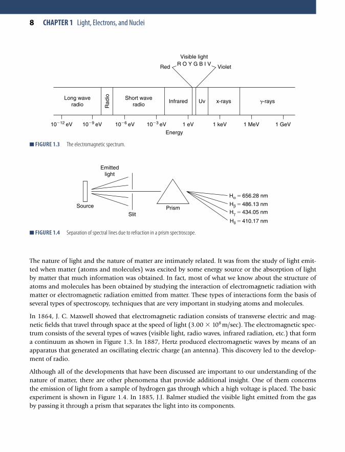
In 1864, J. C. Maxwell showed that electromagnetic radiation consists of transverse electric and mag-netic fi elds that travel through space at the speed of light (3.00 � 10 8 m/sec). The electromagnetic spec-trum consists of the several types of waves (visible light, radio waves, infrared radiation, etc.) that form a continuum as shown in Figure 1.3 . In 1887, Hertz produced electromagnetic waves by means of an apparatus that generated an oscillating electric charge (an antenna). This discovery led to the develop-ment of radio.

Although all of the developments that have been discussed are important to our understanding of the nature of matter, there are other phenomena that provide additional insight. One of them concerns the emission of light from a sample of hydrogen gas through which a high voltage is placed. The basic experiment is shown in Figure 1.4 . In 1885, J.J. Balmer studied the visible light emitted from the gas by passing it through a prism that separates the light into its components.

10�12 eV 10�9 eV 10�6 eV 10�3 eV 1 eV 1 keV 1 MeV 1 GeV

Energy

�-raysx-raysLong wave

radioShort wave

radioInfrared Uv

Visible lightR O Y G B I V

Rad

io

Red Violet

■ FIGURE 1.3 The electromagnetic spectrum.

PrismSource

Slit

Hα � 656.28 nm

Hβ � 486.13 nm

Hγ � 434.05 nm

Hδ � 410.17 nm

Emittedlight

■ FIGURE 1.4 Separation of spectral lines due to refraction in a prism spectroscope.

The four lines observed are as follows.

H nm 6562.8

H nm 4861.3

H nm 434

α

β

γ

� �

� �

� �

656 28

486 13

434 05

.

.

.

Å

Å

00.5 Å

H nm 4101.7 Åδ � �410 17.

This series of spectral lines for hydrogen became known as Balmer’s series, and the wavelengths of these four spectral lines were found to obey the relationship

1 12

12 2λ

� �RnH

⎛⎝⎜⎜⎜

⎞⎠⎟⎟⎟⎟

(1.2)

where λ is the wavelength of the line, n is an integer larger than 2, and R H is a constant known as Rydberg’s constant that has the value 109,677.76 cm � 1 . The quantity 1/ λ is known as the wave number (the number of complete waves per centimeter), which is written as ν ( “ nu bar ” ). From Eq. (1.2) it can be seen that as n assumes larger values, the lines become more closely spaced, but when n equals infi n-ity, there is a limit reached. That limit is known as the series limit for the Balmer series. Keep in mind that these spectral lines, the fi rst to be discovered for hydrogen, were in the visible region of the elec-tromagnetic spectrum. Detectors for visible light (human eyes and photographic plates) were available at an earlier time than were detectors for other types of electromagnetic radiation.

Eventually, other series of lines were found in other regions of the electromagnetic spectrum. The Lyman series was observed in the ultraviolet region, whereas the Paschen, Brackett, and Pfund series were observed in the infrared region of the spectrum. All of these lines were observed as they were emitted from excited atoms, so together they constitute the emission spectrum or line spectrum of hydrogen atoms.

Another of the great developments in atomic physics involved the light emitted from a device known as a black body. Because black is the best absorber of all wavelengths of visible light, it should also be the best emitter. Consequently, a metal sphere, the interior of which is coated with lampblack, emits radiation (blackbody radiation) having a range of wavelengths from an opening in the sphere when it is heated to incandescence. One of the thorny problems in atomic physics dealt with trying to predict the intensity of the radiation as a function of wavelength. In 1900, Max Planck arrived at a satisfactory relationship by making an assumption that was radical at that time. Planck assumed that absorption and emission of radiation arises from oscillators that change frequency. However, Planck assumed that the frequencies were not continuous but rather that only certain frequencies were allowed. In other words, the frequency is quantized . The permissible frequencies were multiples of some fundamental frequency, ν 0 . A change in an oscillator from a lower frequency to a higher one involves the absorption

1.2 The Nature of Light 9

10 CHAPTER 1 Light, Electrons, and Nuclei

of energy, whereas energy is emitted as the frequency of an oscillator decreases. Planck expressed the energy in terms of the frequency by means of the relationship

E h� ν (1.3)

where E is the energy, ν is the frequency, and h is a constant (known as Planck’s constant, 6.63 � 10 � 27 erg sec � 6.63 � 10 � 34 J sec). Because light is a transverse wave (the direction the wave is moving is perpendicular to the displacement), it obeys the relationship

λ ν � c (1.4)

where λ is the wavelength, ν is the frequency, and c is the velocity of light (3.00 � 10 10 cm/sec). By making these assumptions, Plank arrived at an equation that satisfactorily related the intensity and fre-quency of the emitted blackbody radiation.

The importance of the idea that energy is quantized is impossible to overstate. It applies to all types of energies related to atoms and molecules. It forms the basis of the various experimental techniques for studying the structure of atoms and molecules. The energy levels may be electronic, vibrational, or rotational depending on the type of experiment conducted.

In the 1800s, it was observed that when light is shined on a metal plate contained in an evacuated tube, an interesting phenomenon occurs. The arrangement of the apparatus is shown in Figure 1.5 . When the light is shined on the metal plate, an electric current fl ows. Because light and electricity are involved, the phenomenon became known as the photoelectric effect . Somehow, light is responsible for the generation of the electric current. Around 1900, there was ample evidence that light behaved as a wave, but it was impossible to account for some of the observations on the photoelectric effect by con-sidering light in that way. Observations on the photoelectric effect include the following:

1. The incident light must have some minimum frequency (the threshold frequency ) in order for electrons to be ejected.

2. The current fl ow is instantaneous when the light strikes the metal plate.

3. The current is proportional to the intensity of the incident light.

Light

Ejected electrons

� �

■ FIGURE 1.5 Apparatus for demonstrating the photoelectric eff ect.

In 1905, Albert Einstein provided an explanation of the photoelectric effect by assuming that the inci-dent light acts as particles. This allowed for instantaneous collisions of light particles ( photons ) with electrons (called photoelectrons), which resulted in the electrons being ejected from the surface of the metal. Some minimum energy of the photons was required because the electrons are bound to the metal surface with some specifi c binding energy that depends on the type of metal. The energy required to remove an electron from the surface of a metal is known as the work function ( w 0 ) of the metal. The ionization potential (which corresponds to removal of an electron from a gaseous atom) is not the same as the work function. If an incident photon has an energy that is greater than the work function of the metal, the ejected electron will carry away part of the energy as kinetic energy. In other words, the kinetic energy of the ejected electron will be the difference between the energy of the inci-dent photon and the energy required to remove the electron from the metal. This can be expressed by the equation

12

20mv hv w� �

(1.5)

By increasing the negative charge on the plate to which the ejected electrons move, it is possible to stop the electrons and thereby stop the current fl ow. The voltage necessary to stop the electrons is known as the stopping potential . Under these conditions, what is actually being determined is the kinetic energy of the ejected electrons. If the experiment is repeated using incident radiation with a different frequency, the kinetic energy of the ejected electrons can again be determined. By using light having several known incident frequencies, it is possible to determine the kinetic energy of the electrons corre-sponding to each frequency and make a graph of the kinetic energy of the electrons versus ν . As can be seen from Eq. (1.5), the relationship should be linear with the slope of the line being h , Planck’s con-stant, and the intercept is � w 0 . There are some similarities between the photoelectric effect described here and photoelectron spectroscopy of molecules that is described in Section 3.4.

Although Einstein made use of the assumption that light behaves as a particle, there is no denying the validity of the experiments that show that light behaves as a wave. Actually, light has characteristics of both waves and particles, the so-called particle-wave duality . Whether it behaves as a wave or a particle depends on the type of experiment to which it is being subjected. In the study of atomic and molecu-lar structure, it necessary to use both concepts to explain the results of experiments.

1.3 THE BOHR MODEL

Although the experiments dealing with light and atomic spectroscopy had revealed a great deal about the structure of atoms, even the line spectrum of hydrogen presented a formidable problem to the physics of that time. One of the major obstacles was that energy was not emitted continuously as the electron moves about the nucleus. After all, velocity is a vector quantity that has both a magnitude and a direction. A change in direction constitutes a change in velocity (acceleration), and an acceler-ated electric charge should emit electromagnetic radiation according to Maxwell’s theory. If the mov-ing electron lost energy continuously, it would slowly spiral in toward the nucleus and the atom would “ run down. ” Somehow, the laws of classical physics were not capable of dealing with this situation, which is illustrated in Figure 1.6 .

1.3 The Bohr Model 11

12 CHAPTER 1 Light, Electrons, and Nuclei

Following Rutherford’s experiments in 1911, Niels Bohr proposed in 1913 a dynamic model of the hydrogen atom that was based on certain assumptions. The fi rst of these assumptions was that there were certain “ allowed ” orbits in which the electron could move without radiating electromagnetic energy. Further, these were orbits in which the angular momentum of the electron (which for a rotat-ing object is expressed as mvr ) is a multiple of h /2 π (which is also written as � ),

mvr

nhn� �

2π�

(1.6)

where m is the mass of the electron, v is its velocity, r is the radius of the orbit, and n is an integer that can take on the values 1, 2, 3, … , and � is h /2 π . The integer n is known as a quantum number or, more specifi cally, the principal quantum number.

Bohr also assumed that electromagnetic energy was emitted as the electron moved from a higher orbital (larger n value) to a lower one and absorbed in the reverse process.

This accounts for the fact that the line spectrum of hydrogen shows only lines having certain wave-lengths. In order for the electron to move in a stable orbit, the electrostatic attraction between it and the proton must be balanced by the centrifugal force that results from its circular motion. As shown in Figure 1.7 , the forces are actually in opposite directions, so we equate only the magnitudes of the forces.

�

e�

mv2

re2

r 2

■ FIGURE 1.7 Forces acting on an electron moving in a hydrogen atom.

�

e�

■ FIGURE 1.6 As the electron moves around the nucleus, it is constantly changing direction.

The electrostatic force is given by the coulombic force as e 2 / r 2 while the centrifugal force on the elec-tron is mv 2 / r . Therefore, we can write

mv

r r

2 2

2�

e

(1.7)

From Eq. (1.7) we can calculate the velocity of the electron as

v

mr�

e2

(1.8)

We can also solve Eq. (1.6) for v to obtain

v �

nh

mr2π (1.9)

Because the moving electron has only one velocity, the values for v given in Eqs. (1.8) and (1.9) must be equal:

e2

2mr

nh

mr�

π (1.10)

We can now solve for r to obtain

r

n h

me�

2 2

2 24π (1.11)

In Eq. (1.11), only r and n are variables. From the nature of this equation, we see that the value of r , the radius of the orbit, increases as the square of n . For the orbit with n � 2, the radius is four times that when n � 1, etc. Dimensionally, Eq. (1.11) leads to a value of r that is given in centimeters if the constants are assigned their values in the cm-g-s system of units (only h , m , and e have units).

[(g cm /sec ) sec][g(g cm /sec) ]

cm2 2 2

1/2 3/2 2�

(1.12)

From Eq. (1.7), we see that

mv

r2

2�

e

(1.13)

Multiplying both sides of the equation by 1/2 we obtain

12 2

22

mvr

�e

(1.14)

1.3 The Bohr Model 13

14 CHAPTER 1 Light, Electrons, and Nuclei

where the left-hand side is simply the kinetic energy of the electron. The total energy of the electron is the sum of the kinetic energy and the electrostatic potential energy, � e 2 / r .

E mv

r r r r� � � � ��

12 2 2

22 2 2 2e e e e

(1.15)

Substituting the value for r from Eq. (1.11) into Eq. (1.15) we obtain

E

r

m

n h�� ��

e e2 2 4

2 222π

(1.16)

from which we see that there is an inverse relationship between the energy and the square of the value n . The lowest value of E (and it is negative!) is for n � 1 while E � 0 when n has an infi nitely large value that corresponds to complete removal of the electron. If the constants are assigned val-ues in the cm-g-s system of units, the energy calculated will be in ergs. Of course 1 J � 10 7 erg and 1 cal � 4.184 J.

By assigning various values to n , we can evaluate the corresponding energy of the electron in the orbits of the hydrogen atom. When this is done, we fi nd the energies of several orbits as follows:

n E

n E

n E

� � � �

� � � �

� � � �

�

�

1, 21.7 10 erg

2, 5.43 10 erg

3, 2.41 1

12

12

00 erg

4, 1.36 10 erg

5, 0.87 10 erg

6,

12

24

12

�

�

�

� � � �

� � � �

� �

n E

n E

n E �� �

� �

�0.63 10 erg

,

12

n E∞ 0

These energies can be used to prepare an energy level diagram like that shown in Figure 1.8 . Note that the binding energy of the electron is lowest when n � 1 and the binding energy is 0 when n � � .

Although the Bohr model successfully accounted for the line spectrum of the hydrogen atom, it could not explain the line spectrum of any other atom. It could be used to predict the wavelengths of spec-tral lines of other species that had only one electron such as He � , Li 2 � , and Be 3 � . Also, the model was based on assumptions regarding the nature of the allowed orbits that had no basis in classical physics. An additional problem is also encountered when the Heisenberg Uncertainty Principle is considered. According to this principle, it is impossible to know exactly the position and momentum of a par-ticle simultaneously. Being able to describe an orbit of an electron in a hydrogen atom is equivalent

to knowing its momentum and position. The Heisenberg Uncertainty Principle places a limit on the accuracy to which these variables can be known simultaneously. That relationship is

Δ Δ ≥x mv� ( ) � (1.17)

where Δ is read as the uncertainty in the variable that follows. Planck’s constant is known as the fun-damental unit of action (it has units of energy multiplied by time), but the product of momentum multiplied by distance has the same dimensions. The essentially classical Bohr model explained the line spectrum of hydrogen, but it did not provide a theoretical framework for understanding atomic structure.

1.4 PARTICLE-WAVE DUALITY

The debate concerning the particle and wave nature of light had been lively for many years when in 1924 a young French doctoral student, Louis V. de Broglie, developed a hypothesis regarding the nature of particles. In this case, the particles were “ real ” particles such as electrons. De Broglie realized that for electromagnetic radiation, the energy could be described by the Planck equation

E h

hc� �ν

λ (1.18)

n � 1

n � 2

n � 3n � 4n � 5

n � ∞

Lymanseries

Balmerseries

Paschenseries

Brackettseries

■ FIGURE 1.8 An energy level diagram for the hydrogen atom.

1.4 Particle-Wave Duality 15