inputs & assumptions: 2019-2020 integrated resource planning...nov 06, 2019 · based on the...
TRANSCRIPT

1
Inputs & Assumptions:
2019-2020 Integrated Resource Planning
November 2019

2
Table of Contents
Table of Contents
1. Introduction ...................................................................................................................................... 4
1.1 Overview of the RESOLVE model .................................................................................................................... 4
1.2 Document Contents ............................................................................................................................................. 5
1.3 Key Data and Model Updates ........................................................................................................................... 6
2. Load Forecast .................................................................................................................................... 8
2.1 CAISO Balancing Authority Area ...................................................................................................................... 8
2.2 CAISO Balancing Authority Area – Peak Demand .................................................................................... 15
2.3 Other Zones .......................................................................................................................................................... 19
3. Baseline Resources ........................................................................................................................ 21
3.1 Natural Gas, Coal, and Nuclear Generation ............................................................................................... 23
3.2 Renewables .......................................................................................................................................................... 26
3.3 Large Hydro .......................................................................................................................................................... 31
3.4 Energy Storage .................................................................................................................................................... 32
3.5 Demand Response ............................................................................................................................................. 33
4. Candidate Resources ..................................................................................................................... 35
4.1 Natural Gas ........................................................................................................................................................... 35
4.2 Renewables .......................................................................................................................................................... 35
4.3 Energy Storage .................................................................................................................................................... 56
4.4 Demand Response ............................................................................................................................................. 61
5. Pro Forma Financial Model .......................................................................................................... 64
6. Operating Assumptions ................................................................................................................ 65
6.1 Overview ............................................................................................................................................................... 65
6.2 Load Profiles and & Renewable Generation Shapes ............................................................................... 68
6.3 Operating Characteristics ................................................................................................................................ 75
6.4 Operational Reserve Requirements ............................................................................................................. 78

3
6.5 Transmission Topology ..................................................................................................................................... 81
6.6 Fuel Costs .............................................................................................................................................................. 84
7. Resource Adequacy Requirements ............................................................................................. 87
7.1 System Resource Adequacy ............................................................................................................................ 87
7.2 Local Resource Adequacy Constraint ........................................................................................................... 91
7.3 Minimum Retention of Gas-Fired Resources in Local Areas ................................................................ 92
8. Greenhouse Gas Emissions and Renewables Portfolio Standard .......................................... 94
8.1 Greenhouse Gas Constraint ............................................................................................................................ 94
8.2 Greenhouse Gas Accounting .......................................................................................................................... 95
8.3 RPS/SB100 Constraint ....................................................................................................................................... 96

4
1. Introduction
This document describes the key data elements and sources of inputs and assumptions for the
California Public Utilities Commission’s (CPUC’s) 2019-2020 Integrated Resource Planning
(2019-2020 IRP) modeling. It also summarizes the methodology for how different data
components are used by the RESOLVE model to develop the 2019-2020 Reference System
Portfolio.
The inputs, assumptions, and methodologies are applied to create optimal portfolios for the
CAISO electric system that reflect different assumptions regarding load growth, technology
costs and potential, fuel costs, and policy constraints. In some cases, multiple options are
included for use in 2019-2020 IRP scenarios and sensitivities modeling.
1.1 Overview of the RESOLVE model
The high-level, long-term identification of new resources that meet California’s policy goals is
developed using the RESOLVE resource planning model. The CPUC uses RESOLVE to develop
the Reference System Portfolio, a look into the future that identifies a portfolio of new and
existing resources that meets the GHG emissions planning constraint, provides ratepayer value,
and responds to reliability needs. The CPUC uses RESOLVE for the development of the
Reference System Portfolio because it is a publicly available and vetted tool. The CPUC uses the
process of soliciting party feedback on inputs and assumptions to ensure that RESOLVE contains
transparent, publicly available data sources and transparent methodologies to examine the
long-term planning questions posed within the Integrated Resource Planning process.
The CPUC also uses the Strategic Energy Risk Valuation Model (SERVM) as a separate tool more
specifically designed to examine system reliability once an optimal portfolio has been
determined by RESOLVE. RESOLVE and SERVM are used for different but related purposes –
RESOLVE focuses on creating a portfolio of resources, whereas SERVM focuses on system
reliability and production costs. SERVM is a probabilistic model that has more temporal and
geographical granularity than RESOLVE and can therefore provide a higher fidelity assessment
of operational performance. The 2019 IRP Reference System Portfolio development process
includes activities to align the inputs and outputs of RESOLVE and SERVM, to the extent
possible, through the use of common data sources to achieve reasonable agreement in outputs
between the models.
RESOLVE is formulated as a linear optimization problem. It co-optimizes investment and
dispatch for a selected set of days over a multi-year horizon to identify least-cost portfolios for
meeting carbon emission reduction targets, renewables portfolio standard goals, reliability
during peak demand events, and other system requirements. RESOLVE typically focuses on

5
developing portfolios for one zone, in this case the CAISO Balancing Authority Area, but
incorporates a representation of neighboring zones in order to characterize transmission flows
into and out of the region of interest. Zone in this context refers to a geographic region that
consists of a single balancing authority area (BAA) or a collection of BAAs in which RESOLVE
balances the supply and demand of energy. The CPUC IRP version of RESOLVE includes six
zones: four zones capturing California balancing authorities and two zones that represent
regional aggregations of out-of-state balancing authorities.1 The CAISO zone in RESOLVE
represents the CAISO balancing authority area.
RESOLVE can solve for:
• Optimal investments in renewable resources, energy storage technologies, demand
response resources, distributed energy resources, and new thermal gas plants, as well
as retention of existing thermal resources.
Subject to the following constraints:
• An annual constraint on delivered renewable energy that reflects Renewables Portfolio
Standard (RPS) policy;
• An annual constraint on greenhouse gas emissions;
• An annual Planning Reserve Margin (PRM) constraint to maintain capacity adequacy and
reliability;
• Operational restrictions on generators and resources;
• Hourly load and reserve requirements; and
• Constraints on the ability to develop specific new resources.
RESOLVE optimizes the buildout of new resources ten or more years into the future,
representing the fixed costs of new investments and the costs of operating the CAISO system
within the broader footprint of the Western Electricity Coordinating Council (WECC) electricity
system.
1.2 Document Contents
The remainder of this document is organized as follows:
1 A seventh resource-only zone was added in the 2019 IRP to simulate dedicated imports from Pacific Northwest hydroelectric resources. This zone does not have any load and does not represent a BAA.

6
• Section 2 (Load Forecast) documents the assumptions and corresponding sources used
to derive the forecast of load in CAISO and the WECC, including the impacts of demand-
side programs, load modifiers, and the impacts of electrification.
• Section 3 (Baseline Resources) summarizes assumptions on baseline resources. Baseline
resources are existing or planned resources that are assumed to be operational in the
year being modeled.
• Section 4 (Candidate Resources) discusses assumptions used to characterize the
potential new resources that can be selected for inclusion in the optimized, least-cost
portfolio. Candidate resources are incremental to baseline resources.
• Section 5 (Pro Forma) describes the financial model used to calculate levelized fixed
costs of candidate resources in RESOLVE.
• Section 6 (Operating Assumptions) presents the assumptions used to characterize
hourly electricity demand and the operations of each of the resources represented in
RESOLVE’s internal hourly production simulation model.
• Section 7 (Resource Adequacy Requirements) discusses the constraints imposed on the
RESOLVE portfolio to ensure system and local reliability needs are met, as well as
assumptions regarding the contribution of each resource towards these requirements.
• Section 8 (Greenhouse Gas Emissions and Renewables Portfolio Standard) discusses
assumptions and accounting used to characterize constraints on portfolio greenhouse
gas emissions and renewables portfolio standard targets.
1.3 Key Data and Model Updates
Since the publication of the “CPUC 2017 IRP RESOLVE Documentation: Inputs & Assumptions”2
in September 2017, CPUC staff and its consultant Energy and Environmental Economics, Inc.
(E3) implemented numerous updates to RESOLVE model functionality, inputs, and assumptions.
Key updates include:
• Updating the Load Forecast assumptions to align with the CEC 2018 Integrated Energy
Policy (IEPR) California Energy Demand Forecast Update (Section 2).
• Adding updates to allow for modeling out to 2045, including PATHWAYS load
assumptions through 2045 (Section 2.1.9).
• Updating the Baseline Resource assumptions to the most recent data available on
existing and planned resources within and outside of CAISO (Section 3.0).
2 Found at: http://cpuc.ca.gov/uploadedFiles/CPUCWebsite/Content/UtilitiesIndustries/Energy/EnergyPrograms/ElectPowerProcurementGeneration/irp/AttachmentB.RESOLVE_Inputs_Assumptions_2017-09-15.pdf

7
• Enabling RESOLVE to retain the economically optimal level of dispatchable gas
generators (Section 3.1.1).
• Revising the capital cost assumptions of renewable technologies (Section 4.2).
• Revising the capital cost assumptions of battery storage technologies (Section 4.3).
• Adding a declining storage ELCC curve to reflect lower battery storage capacity value at
higher levels of battery penetration (Section 7.1.5).
• Updating candidate renewable resource transmission zones and transmission
capabilities, including the ability to model multiple simultaneous (“nested”)
transmission constraints (Sections 4.2.1 and 4.2.7).
• Adding behind-the-meter (BTM) storage as a candidate resource (Section 4.3).
• Adding near-term deployment limits for Candidate Solar and Shed DR resources
(Sections 4.2.5 and 4.4.1).

8
2. Load Forecast
2.1 CAISO Balancing Authority Area
The primary source for CAISO load forecast inputs (both peak demand and total energy) in the
2019-2020 Reference System Portfolio is the CEC’s 2018 Integrated Energy Policy Report (IEPR)
Demand Forecast Update.3 The CEC’s 2018 Deep Decarbonization in a High Renewable Future
report is also used to provide long-term forecasts for the 2045 Framing Studies.
Many components of the CEC IEPR demand forecast are broken out so that the distinct hourly
profile of each of these factors can be represented explicitly in modeling. The components are
referred to in this document as “demand-side modifiers.” Hourly profiles for demand-side
modifiers are discussed in Section 6.2.1.
Demand-side modifiers include:
• Electric vehicles
• Building electrification4
• Other electrification
• Behind-the-meter PV
• Non-PV self-generation (predominantly behind-the-meter combined heat and power)
• Energy efficiency
• Time of use (TOU) rate impacts
Data sources for demand-side modifier assumptions are discussed in subsequent sections.
Demand forecast inputs are frequently presented as demand at the customer meter. However,
the RESOLVE dispatch optimization uses demand at the generator bus-bar. Consequently,
demand forecasts at the customer meter are grossed up for transmission & distribution losses
based on the average losses across the CAISO zone assumed in the CEC’s IEPR Demand Forecast
of 7.24%.
3 In the 2017-2018 IRP cycle, most of the demand data was extracted from IEPR Forms 1.1c, 1.5a, 1.5b, and 1.2. In the 2019-2020 IRP cycle, 2018 IEPR workbooks breaking out demand and demand modifier components for the CAISO area, hourly profiles, and installed capacity for BTM resources were also used to develop inputs for IRP modeling. 4 Building electrification estimates are not currently included in the 2018 IEPR’s Demand Forecast Update but are available from the CEC’s 2018 Deep Decarbonization in a High Renewables Future.

9
Baseline Consumption
Baseline consumption refers to a counterfactual forecast of electricity consumption that
captures economic and demographic changes in California but does not include the impact of
demand-side modifiers. The baseline consumption forecast used in the 2019-2020 IRP cycle is
derived from retail sales reported in the CEC’s 2018 IEPR Demand Forecast along with
accompanying information on the magnitude of embedded demand-side modifiers. Creating a
baseline consumption forecast enables different combinations of demand-side modifiers to be
used in the IRP, including combinations that are not explored in the IEPR Demand Forecast. The
derivation of baseline consumption from the retail sales forecast is shown in Table 1.
Table 1. Derivation of Baseline Consumption from the CEC IEPR Demand Forecast (GWh)
Component 2020 2022 2026 2030
CEC 2018 IEPR Retail Sales 207,518 207,673 206,438 202,653
+ Mid AAEE 5,930 10,186 19,550 27,940
+ Behind-the-Meter PV 16,931 21,537 28,503 35,123
+ Behind-the-Meter CHP 13,637 13,655 13,638 13,595
+ Other Self Generation5 751 737 708 681
- TOU rate effects 0 27 31 35
- Electric Vehicles 4,578 6,817 10,727 13,567
- Other Transport Electrification 222 306 520 683
= Baseline Consumption 239,966 246,638 257,559 265,707
Electric Vehicles
The 2019-2020 IRP cycle includes five options for forecasting future electric vehicle demand in
the 2019-2020 IRP cycle. The first two options are based directly on the IEPR Mid and High
Demand forecast. The remaining three options are based on scenarios from the CEC 2018 Deep
Decarbonization report, which extend beyond the 2030 timeframe to reflect different levels of
electrification. Post-2030 loads are described in section 2.1.9.
5 Non-PV, Non-CHP Self Generation. Includes storage losses.

10
Table 2. Electric vehicle forecast options (GWh)
RESOLVE Scenario Setting 2020 2022 2026 2030
CEC 2018 IEPR - Mid Demand 4,578 6,817 10,727 13,567
CEC 2018 IEPR - High Demand 4,765 7,205 12,040 15,160
CEC 2018 Deep Decarbonization - High Biofuels 1,110 1,946 5,862 11,099
CEC 2018 Deep Decarbonization - High Electrification 1,110 1,947 5,838 11,442
CEC 2018 Deep Decarbonization - High Hydrogen 1,110 1,947 5,838 11,442
Building Electrification
Two options for future building electrification demand are included in the 2019-2020 IRP cycle.
The first reflects the IEPR assumption of no incremental building electrification, and the second
is based on the assumptions in the CEC Deep Decarbonization report.
Table 3. Building electrification forecast options (GWh)
RESOLVE Scenario Setting 2020 2022 2026 2030
No Incremental Building Electrification6 - - - -
CEC 2018 Deep Decarbonization 7 - - 255 3,023
Other Transport Electrification
The forecast options for electrification of “other” end uses (e.g. ports, and airport ground
equipment) is based on the CEC 2018 IEPR Demand Forecast.
Table 4. Other transport electrification forecast options (GWh)
RESOLVE Scenario Setting 2020 2022 2026 2030
No Incremental Other Transport Electrification - - - -
CEC 2018 IEPR - Mid Demand 222 306 520 683
6 This is consistent with the IEPR demand forecast which does not include incremental building electrification, and
with the CARB 2016 Scoping Plan “SP” scenario. In the RESOLVE scenario tool workbook, an additional building electrification forecast “None through 2030” is included for post-2030 sensitivity analysis. 7 The High Electrification, High Hydrogen and High Biofuels Scenarios from the CEC’s 2018 “Deep Decarbonization in a High Renewables Future” have the same building electrification assumptions.

11
CEC 2018 Deep Decarbonization - High Biofuels 1,198 1,734 3,596 6,615
CEC 2018 Deep Decarbonization - High Electrification 1,198 1,734 3,596 6,617
CEC 2018 Deep Decarbonization - High Hydrogen 1,127 1,590 3,054 5,107
Behind-the-Meter PV
The 2019-2020 IRP scenarios include three options for behind-the-meter (BTM) PV adoption,
each of which is based on the CEC’s IEPR Demand Forecast. These options—Low, Mid, and
High—correspond to the 2018 High, Mid, and Low Demand Forecasts. Note that the IRP Low
BTM PV forecast is based on the IEPR High Demand Forecast and the IRP High BTM PV forecast
is based on the IEPR Low Demand Forecast. The naming of the IEPR forecasts corresponds to
the relative level of retail load in each of the forecasts, and higher amounts of BTM PV yield
lower retail load.
Table 5. Behind-the-meter PV forecast options (GWh)
RESOLVE Scenario Setting 2020 2022 2026 2030
CEC 2018 IEPR - Low PV 15,306 17,429 20,493 23,873
CEC 2018 IEPR - Mid PV 16,797 20,897 26,806 32,466
CEC 2018 IEPR - High PV 18,314 24,424 33,245 41,318
The 2018 IEPR includes forecasts for “Additional Achievable Photovoltaic” (AAPV) adoption to
account for behind-the-meter PV adoption attributable to 2019 Title 24 regulations for new
homes. AAPV adoption is incremental to behind-the-meter PV adoption included in the IEPR
demand forecast, and includes low-, mid-, and high- scenarios, shown in the table below.
Table 6. Additional Achievable Photovoltaic (AAPV) forecast options (GWh)
RESOLVE Scenario Setting 2020 2022 2026 2030
CEC 2018 IEPR - High-Low AAPV 148 768 2,127 3,345
CEC 2018 IEPR - Mid-Mid AAPV 134 640 1,697 2,657
CEC 2018 IEPR - Low-High AAPV 120 513 1,272 1,980

12
Behind-the-meter CHP and Other Non-PV Self Generation
The forecast of non-PV self-generation is based on the CEC 2018 IEPR Demand Forecast. On-site
combined heat & power (CHP) that does not export to the grid makes up the majority of this
component. Because emissions from BTM CHP are counted towards total electric sector
emissions, the portion of BTM CHP is separated from the total non-PV self-generation. The IEPR
primarily models on-site CHP using projections based on past on-site CHP generation data. CHP
units that export energy to the grid are separately discussed in section 3. Forecasts for BTM
CHP and the remaining non-PV self-generation are shown in the tables below.
Table 7. Forecast of Behind-the-meter CHP (GWh)
Scenario Setting 2020 2022 2026 2030
CEC 2018 IEPR - Mid Demand 13,637 13,655 13,638 13,595
Table 8. Forecast of other non-PV on-site self-generation (GWh)
Scenario Setting 2020 2022 2026 2030
CEC 2018 IEPR - Mid Demand 751 737 708 681
Energy Efficiency
The 2019-2020 IRP cycle includes three options for varying levels of energy efficiency
achievement among CAISO load-serving entities based on the scenarios included in the CEC’s
2018 IEPR Demand Forecast.8 “Additional Achievable Energy Efficiency” (AAEE) refers to
efficiency savings beyond current committed programs. The options presented below are based
on the IEPR Mid Demand Forecast - other IEPR AAEE scenarios could be included in sensitivity
analyses as necessary.
Table 9. Energy efficiency forecast options (GWh)
RESOLVE Scenario Setting 2020 2022 2026 2030
CEC 2018 IEPR - High Low AAEE 4,882 7,948 14,781 21,113
CEC 2018 IEPR - Mid Mid AAEE 5,930 10,186 19,550 27,940
8 AAEE scenarios in the 2018 are consistent with the 2017 Updated Demand Forecast AAEE Scenarios.

13
CEC 2018 IEPR - Low High AAEE 6,432 11,197 22,277 32,724
Time-of-Use Rate Impacts
The 2019-2020 cycle includes two options for representing different impacts of residential
time-of-use (TOU) rate implementation on retail load. The first assumes no impact to load
shape. The second corresponds to mid residential TOU scenarios from CEC’s IEPR Demand
Forecast. As modeled, TOU rates modify the hourly load profile but have little impact on annual
load.
Table 10. Residential TOU rate implementation load impacts (GWh)
RESOLVE Scenario Setting 2020 2022 2026 2030
None — — — —
CEC 2018 IEPR 0 27 31 35
2045 Framing Study Pathways loads
The CEC’s 2018 Deep Decarbonization in a High Renewable Future report is used to provide
long-term forecasts for the 2045 Framing Studies. E3’s PATHWAYS model provides load
forecasts for the three 2045 framing scenarios: High Electrification, High Biofuels and High
Hydrogen. Each scenario follows the PATHWAYS assumptions for load modifiers, including
electric vehicles, other transport electrification, building electrification, and hydrogen
production. Statewide PATHWAYS load is converted to CAISO load in the 2045 framing
scenarios assuming an 81% load share. The High Electrification scenario is picked as the default
scenario in the 2045 framing study because it provides a balanced decarbonization pathway
between electrification and low-carbon fuels with relatively low costs and commercially
available technologies.
All three scenarios follow the same assumptions on energy efficiency and baseline
consumption. Energy efficiency is scaled up over time from 2030 IEPR Mid Mid AAEE values to
reach PATHWAYS energy efficiency assumptions in 2050. PATHWAYS does not report baseline
consumption directly, but rather reports baseline consumption net of energy efficiency. A
baseline consumption forecast is created by combining efficiency assumptions with PATHWAYS
outputs. Baseline consumption, as a result, grows at a similar rate as in the CEC 2018 IEPR Mid
Demand forecast (~0.5% per year through 2050).

14
Table 11. CEC Pathways High Biofuels Load Forecast (GWh)
RESOLVE Scenario Setting 2020 2022 2026 2030 2045
Baseline Consumption 239,966 246,638 257,559 265,707 286,572
Electric Vehicles 1,110 1,946 5,862 11,099 30,485
Other Transport Electrification 1,198 1,734 3,596 6,615 26,852
Building Electrification - - 255 3,023 35,104
Hydrogen Production (GWh) 203 331 611 579 986
Energy Efficiency (5,930) (10,186) (19,550) (27,940) (46,390)
Total 236,547 240,463 248,333 259,083 333,609
Table 12. CEC Pathways High Electrification Pathways Load Forecast (GWh)
RESOLVE Scenario Setting 2020 2022 2026 2030 2045
Baseline Consumption 239,966 246,638 257,559 265,707 286,572
Electric Vehicles 1,110 1,947 5,838 11,442 38,427
Other Transport Electrification 1,198 1,734 3,596 6,617 28,209
Building Electrification - - 255 3,023 35,104
Hydrogen Production 276 499 1,563 4,476 31,913
Energy Efficiency (5,930) (10,186) (19,550) (27,940) (46,390)
Total 236,620 240,632 249,261 263,325 373,835
Table 13. CEC Pathways High Hydrogen Load Forecast (GWh)
RESOLVE Scenario Setting 2020 2022 2026 2030 2045
Baseline Consumption 239,966 246,638 257,559 265,707 286,572
Electric Vehicles 1,110 1,947 5,838 11,442 38,427
Other Transport Electrification 1,127 1,590 3,054 5,107 17,013
Building Electrification - - 255 3,023 35,104
Hydrogen Production 279 506 1,578 4,559 89,226
Energy Efficiency (5,930) (10,186) (19,550) (27,940) (46,390)

15
Total 236,552 240,495 248,734 261,898 419,952
2.2 CAISO Balancing Authority Area – Peak Demand
To ensure that the electricity system has adequate resources to reliably operate the system
during the hours of highest demand, RESOLVE’s planning reserve margin constraint guarantees
that all portfolios have at least a 15% margin above the 1-in-2 net peak demand in all modeled
years. The peak demand of the system can significantly impact resource portfolio selection by
increasing the value of resources that can produce energy during peak periods.
Both the timing and magnitude of peak demand are impacted by changes in demand-side
modifiers, including but not limited to behind-the-meter solar and storage, energy efficiency,
and new loads from electrification of transportation and other fossil-fueled end uses.
Calculation of system net peak demand takes into account the combined impact of all of the
demand-side modifiers.
Mid Managed Peak Demand Projection - Through 2030
To be consistent with the use of a Single Forecast Set9 for electric resource planning activities,
the CAISO managed net peak through 2030 is calculated using CEC 2018 IEPR “Mid case”
assumptions on the annual level of demand and various demand modifiers. An hourly 8760
timeseries of CAISO electric demand – net of demand modifiers – for the years 2018-2030 is
developed by combining normalized hourly demand shapes from the 2018 IEPR with annual
demand projections. Peak demand impacts for individual demand modifiers are not calculated
for the IEPR Mid case because interactive effects between hourly shapes and the timing of peak
demand result in demand modifier peak impacts that are interdependent and non-linear. As
outlined below, all demand modifiers with an hourly shape are added or subtracted from the
hourly consumption forecast, resulting in a peak demand in each year that is referred to as the
“Managed Peak” demand.
CAISO Hourly Consumption Load: Mid Baseline
+ Other Electrification: Mid (included in hourly consumption load)
9 Final 2018 Integrated Energy Policy Report Update, Volume II- Clean Version:
https://efiling.energy.ca.gov/getdocument.aspx?tn=226392

16
- Non-PV Self Generation (predominantly BTM CHP) (included in hourly
consumption load)
- Behind-the-Meter (BTM) Storage Peak Impact (included in hourly consumption
load)
+ Load from Vernon and SVP data centers
+ Time-Of-Use: Mid (can increase or decrease hourly demand)
+ Climate Change Impacts: Mid (can increase or decrease hourly demand)
+ Light-Duty Electric Vehicles: Mid
- Additional Achievable Energy Efficiency: Mid-Mid
- Committed BTM PV: Mid
- Additional Achievable BTM PV: Mid-Mid
= CAISO Managed Net Mid Peak, Coincident, through 2030, excluding Load Modifying
Demand Response (LMDR)
- LMDR: Mid
= CAISO Managed Net Mid Peak, Coincident, through 2030
Notes:
• The peak demand impacts of Other Electrification and non-PV Self Generation (including
BTM combined heat and power and BTM storage) are embedded in the CEC IEPR's
hourly consumption load shape, and therefore do not have separate hourly profiles.
• The CEC represents the peak discharge capability of BTM storage as the installed BTM
storage capacity, reduced by a 1% per year degradation rate (cumulative), and then de-
rated to 90% output during peak.
• The peak demand impacts of load modifying demand response are not represented
using an hourly load profile and are instead subtracted from the Managed Peak.
Peak Demand for Demand Sensitivities - Through 2030
The analysis above creates peak demand values for a central set of “Mid” demand assumptions.
Sensitivity analysis on components of the demand forecast requires peak demand forecasts
consistent with changes in the underlying demand components. The peak demand difference
from the “Mid” demand assumptions is calculated for the following demand modifiers:
• Baseline Consumption: High Demand

17
• Electric Vehicles: High Demand
• Energy Efficiency: High Low AAEE
• Energy Efficiency: Low High AAEE
• BTM PV: Low PV + High-Low AAPV (“Low” BTM PV)
• BTM PV: High PV + Low-High AAPV (“High” BTM PV)
The peak demand difference from Mid is calculated for each of the above demand modifiers
individually. The hourly (8760) profile of each demand modifier is adjusted to the level of
annual demand in the alternate IEPR forecast. For example, the peak impact of the High
Demand baseline is calculated by increasing hourly baseline demand to reflect annual values in
the IEPR High Load baseline forecast, while keeping all other demand modifiers at Mid levels.
The new peak demand value in each year (the maximum of the annual hourly timeseries for
CAISO Managed Net load) is subtracted from the peak demand value from the central set of
“Mid” demand assumptions, which has Baseline consumption at “Mid” levels.
Peak Demand for Post-2030 Years
RESOLVE simulations require peak demand forecasts for every year that is simulated. The CEC
2018 IEPR forecasts demand through 2030, but some scenarios explored in the 2019 IRP extend
past 2030, requiring an extrapolation of the peak demand to years beyond 2030.
To develop peak demand forecasts for years after 2030 for baseline consumption, electric
vehicles, energy efficiency, and BTM PV, information from the peak demand sensitivities is used
to calculate a normalized peak demand impact. For each of the demand modifiers, the peak
demand difference from Mid in the year 2030 is normalized to the increase or decrease in
annual demand, resulting in the peak demand increase per unit of demand modifier (Δ MWpeak
/ Δ GWhannual). This factor is used to calculate the increase or decrease in peak demand
resulting from a change in annual demand relative to 2030.
Building Electrification and Other Transportation Peak Demand Impact
The peak impact (Δ MWpeak / Δ GWhannual) of building and other transportation electrification
are calculated using an extrapolated hourly demand projection for the year 2050. The peak
demand impact is calculated by adding or removing a small amount of demand and observing
the change in peak.
Peak demand adjustment for modeling BTM PV and Storage as supply side
Resource adequacy needs are typically calculated with BTM resources represented on the
demand side. In this framework, BTM resources contribute to system peak needs by reducing
the 1:2 system peak. RESOLVE represents BTM PV and Storage resources as supply-side
resources in both hourly dispatch and resource adequacy retirements. Two adjustments are

18
made to the MW value of RESOLVE’s planning reserve margin constraint that align the supply-
side treatment of these resources with the typical demand-side resource adequacy
representation:
• The peak reduction from each resource is added back to RESOLVE’s planning reserve
margin MW need. This is necessary to avoid double counting the peak reduction of BTM
PV and storage.
o The peak reduction from BTM PV is calculated by removing Committed and
AAPV hourly production profiles from the “Mid” load profile and recalculating
the peak demand in each year.
o The peak reduction from BTM storage does not vary by hour, so the BTM storage
peak reduction is added back to the planning reserve margin target directly.
• Demand-side resources reduce the capacity needed above the peak load because the
planning reserve margin (PRM) is calculated as a percentage (typically 15%) above the
managed load peak. Consistent with Resource Adequacy accounting, demand-side
resources reduce the managed load peak, so the 15% margin above 1-in-2 peak demand
is not held for these resources. When modeling demand-side resources on the supply
side, the planning reserve margin that is input into RESOLVE is reduced by the PRM
percentage multiplied by the MW of peak reduction from BTM resources modeled on
the supply-side in RESOLVE.
Figure 2.1. Translation of demand-side resources to the supply-side in RESOLVE. Diagram is conceptual
and is not to scale. The heavy black line indicates the PRM MW target.
Pe
ak C
apac
ity
(MW
)
PRM Calculation with
BTM resources on the
demand-side
PRM Calculation without
PRM margin reduction for
BTM (not used)
PRM Calculation in RESOLVE -
with BTM resources on the
supply-side
(4) 15% PRM on supply-side BTM resources
(15% * (3))
(PRM margin from BTM resources modeled
as supply not included)
(3) Peak Capacity reduction from BTM PV
and Storage, added back to supply side (3) Peak Capacity reduction from BTM PV and
Storage, added back to supply side
(2) 15% PRM on Managed Peak
(15% * (1))
(2) 15% PRM on Managed Peak
(15% * (1))
(2) 15% PRM on Managed Peak
(15% * (1))
(1) Managed Net Load Peak (1) Managed Net Load Peak (1) Managed Net Load Peak

19
2.3 Other Zones
RESOLVE uses a zonal transmission topology to simulate flows among the various regions in the
Western Interconnection. RESOLVE includes six zones: four zones capturing California balancing
authorities (Balancing Authority of Northern California (BANC), California Independent System
Operator (CAISO), Los Angeles Department of Water and Power (LADWP), and Imperial
Irrigation District (IID)) and two zones that represent regional aggregations of out-of-state
balancing authorities.10 The constituent balancing authorities included in each RESOLVE zone
are shown in Table 45 (Section 6.5).
Demand forecasts for zones outside CAISO are developed by a process similar to CAISO
forecasts. Forecasts are taken from two sources:
• For each of the zones within California (LADWP, BANC, and IID) but external to CAISO,
the CEC’s IEPR net energy for load is forecasted using Single Forecast Set assumptions,
including mid demand baseline, mid AAEE, and mid AAPV.11
• For the zones outside of California (the Pacific Northwest and the Southwest), WECC’s
2028 Anchor Data Set (ADS) Phase 2 V1.2 is used as the basis for load projections. Sales
forecasts net of demand-side modifiers are combined with available information in the
ADS related to demand-side modifier and consumption forecasts. This data is then be
aggregated to the RESOLVE zones.
The demand forecasts for each non-CAISO zone are grossed up for transmission and
distribution losses. Demand forecasts for zones outside CAISO are shown in the table below.
10 The 2019 IRP includes an additional resource-only zone to simulate dedicated Pacific Northwest Hydro imports. This zone does not have any load and is not included here. 11 See for Section 6.5 for details on the zonal topology used in RESOLVE.

20
Table 14. Non-CAISO Net Energy for Load - grossed up for T&D losses (GWh)
RESOLVE Zone 2020 2022 2026 2030 2045
NW 240,828 243,368 248,416 253,973 273,690
SW 142,457 146,338 152,407 158,873 183,496
LDWP 27,417 27,401 26,595 25,622 22,638
IID 3,883 3,895 3,888 3,861 3,767
BANC 19,032 18,979 18,690 18,651 18,353

21
3. Baseline Resources
Baseline resources are resources that are currently online or are contracted to come online
within the planning horizon. Being “contracted” refers to a resource holding signed contract/s
with an LSE/s for much of its energy and capacity for a significant portion of its useful life. The
contracts refer to those approved by the CPUC and/or the LSE’s governing board, as applicable.
These criteria indicate the resource is relatively certain to come online.
The capacity of baseline resources is an input to capacity expansion modeling, as opposed to
candidate resources, which are selected by the model and are incremental to the baseline. For
some resources, baseline resource capacity is reduced over time to reflect announced
retirements. An estimation of baseline resource capital costs is used when calculating total
revenue requirements and electricity rates.
Baseline resources include:
• Existing resources: Resources that have already been built and are currently
available, net of expected future retirements.
• Resources under development: Resources that have contracts approved by the
CPUC or the board of a community choice aggregator (CCA) or energy service
provider (ESP) and are far enough along in the development process that it is
reasonable to assume that the resource will be completed. To reflect the potential
for project failure these resources are discounted by 5 percent, a value based on RPS
Procurement Plans and stakeholder feedback.
• Resources not optimized: Future projected resource additions that are expected, but
not appropriate for optimization (e.g., achievement of the CPUC storage target).
• Resources under development in non-CAISO balancing areas: The IRP process does
not optimize resource additions for balancing areas outside CAISO, but changes in
the generation portfolio of balancing areas outside of CAISO may influence portfolio
selection within the CAISO area. Consequently, baseline resources are added to
other balancing areas to meet policy and reliability targets outside of CAISO.
Baseline resources are assembled from the primary sources listed in Error! Reference source
not found. and are further described below.

22
Table 15. Data Sources for Baseline Resources
Zone Online Status Generator type Dataset used
In CAISO Existing Renewable, Storage,
and Non-Renewable
CAISO Master Generating Capability
List, CAISO Master File
In CAISO Under
development
Renewable and Storage RPS Contract Database and data
requests
In CAISO Under
development
Non-Renewable WECC ADS
Out of CAISO Existing and under
development
Renewable, Storage
and Non-Renewable
WECC ADS, with supplemental solar
resources for SB100 compliance
● The list of generators currently operational inside the CAISO is compiled from the CAISO
Master Generating Capability List12. These generators serve load inside CAISO and are
composed of renewable and non-renewable generation resources, as well as some
demand response resources. The CAISO Master Generating Capability List information is
supplemented by the CAISO Master File, a confidential data set with unit-specific
operational attributes. The CAISO Master File also includes information related to
dynamically scheduled generators. These generators are physically located outside of
the CAISO but can participate in the CAISO market as if they were internal to CAISO.
However, because they have no obligation to sell into CAISO they are modeled as
unspecified imports and do not have special priority given to their energy dispatch.
● Future renewable generators that will serve IOU-related CAISO load are compiled from
the January 2019 version of the RPS contracts database maintained by CPUC staff and
supplemented by data requests from CCAs and ESPs.
● The TEPPC ADS is used for renewable generators outside of CAISO. For LADWP, BANC,
and IID, additional solar resources are added to the portfolio if TEPPC ADS renewable
resources fall short of the amount of renewable generation needed under a 60% RPS by
2030.
● For generators outside of CAISO, including areas within California such as LADWP and
SMUD, generator listings and their associated operating information are taken from the
most current version of the WECC’s 2028 Anchor Data Set (ADS) Phase 2 V1.2.
12 Available at: http://oasis.caiso.com/mrioasis/logon.do

23
3.1 Natural Gas, Coal, and Nuclear Generation
Modeling Methodology
Natural gas, coal, and nuclear resources are represented in RESOLVE by a limited set of
resource classes by zone, with operational attributes set at the capacity weighted average for
each resource class in that zone. The capacity weighted averages are calculated from individual
unit attributes available in the CAISO Master File or the WECC ADS. The following resource
classes are modeled: Nuclear, Coal, Combined Cycle Gas Turbine (CCGT), Gas Steam, Peaker,
Reciprocating Engine, and Combined Heat and Power (CHP).
To more accurately reflect different classes of gas generators in the CAISO zone, CAISO’s gas
generators are further divided into subcategories. Resources are grouped and differentiated
into subcategories based on natural breakpoints in operating efficiency observed in the
distribution of data within class averages:
• The CCGT generator category is divided into two subcategories based on generator
efficiency: higher efficiency units are represented as “CAISO_CCGT1” and lower
efficiency units are represented as “CAISO_CCGT2”.
• The Peaker generator category is the aggregation of natural gas frame and
aeroderivative technologies and is divided into two subcategories: higher efficiency
units are represented as “CAISO_Peaker1” and lower efficiency units are represented as
“CAISO_Peaker2”.
• The “CAISO_ST” generator category represents the existing fleet of steam turbines, all
of which are scheduled to retire by default at the end of 2020 to achieve compliance
with the State Water Board’s Once-Through-Cooling (OTC) regulations. Sensitivity
analysis explores alternative retirement assumptions for OTC steam units.
• The “CAISO_Reciprocating_Engine” generator category represents existing gas-fired
reciprocating engines on the CAISO system.
• The “CHP” generator category represents non-dispatchable cogeneration facilities with
thermal hosts, which are modeled as firm resources in RESOLVE. “Firm” refers to
around-the-clock power production at a constant level.
The capacity of fossil-fueled and nuclear thermal generators that have formally announced
retirement are removed from baseline thermal capacity using the announced retirement
schedule.

24
Economic Retention
In the 2017 IRP, existing thermal resources were assumed to be available indefinitely unless
retirement had already been announced. In the 2019-2020 IRP, the RESOLVE model has been
updated to determine the optimal level of dispatchable gas resources to retain that minimizes
overall CAISO system costs.
Fixed operations and maintenance costs (fixed O&M) of baseline gas-fired resources are
considered in RESOLVE’s optimization logic such that dispatchable gas generators will only be
retained by the model, subject to reliability constraints, if it is cost-effective to do so. Fixed
O&M costs are derived from NREL’s 2018 Annual Technology Baseline.13
• Retention decisions are made for CCGTs, Peakers, and Reciprocating Engines.
• Gas resources located in local capacity regions are retained to maintain local reliability
(Section 7.3)
• Combined heat and power (CHP) facilities are retained indefinitely due to the presence
of a thermal host.
• OTC plants (CAISO_ST) are already scheduled for retirement and are retired on
schedule. Retention decisions for these plants are not made by RESOLVE.
Note that RESOLVE's thermal economic retention functionality assesses whether it is economic
to retain gas capacity for CAISO ratepayers, but does not assess whether gas capacity should
retire. Other offtakers may contract with gas plants balanced by CAISO, even if CAISO
ratepayers do not. In addition, gas plant operators may choose to keep plants online without a
long-term contract.
CAISO Resources
Baseline natural gas, coal, and nuclear resources serving CAISO load are drawn from a
combination of the CAISO Master Generating Capability List and the CAISO Master File. Planned
new generation for the CAISO area is taken from the WECC 2028 Anchor Data Set.
Table 16. Baseline Conventional Resources in the CAISO balancing area (MW)
Resource Class 2020 2022 2026 2030
CHP 2,296 2,296 2,296 2,296
13 https://atb.nrel.gov/electricity/2018/

25
Resource Class 2020 2022 2026 2030
Nuclear* 2,935 2,935 635 635
CCGT1 12,049 13,333 13,333 13,333
CCGT2 2,928 2,928 2,928 2,928
Coal** 480 480 - -
Peaker1 4,914 4,914 4,914 4,914
Peaker2 3,683 3,683 3,683 3,683
Advanced CCGT - - - -
Aero CT - - - -
Reciprocating Engine 255 255 255 255
ST (default) 4,577 - - -
Total 34,118 30,824 28,044 28,044
*Diablo Canyon units are assumed to retire in 2024 and 2025. The share of Palo Verde Nuclear Generating Station capacity
contracted to CAISO LSEs is included in all years and is modeled within CAISO in RESOLVE. After retirement of Diablo Canyon in
2025, all remaining CAISO nuclear capacity is from Palo Verde.
** Dedicated imports from the Intermountain Power Plant, located in Utah.
There are three scenarios that reflect different assumptions about the timing and amount of
OTC retirements for the 2019-20 RSP. Under full extension, all OTC plants that are assumed to
be operational at the end of 2020 are continued through 2023. Under the partial extension, 1,4
GW of OTC plants are assumed to retire in 2021 and the remaining continue through 2023.
Resource Class 2020 2022 2026 2030
ST (default) 4,577 - - -
ST (partial extension) 4,577 2,289 - -
ST (full extension) 4,577 3,733 - -
Other Zones
For zones external to the CAISO, the baseline gas, coal, and nuclear generation fleet is based on
the WECC 2028 ADS. The ADS is used to characterize the existing and anticipated future
generation fleet in each non-CAISO zone. The ADS uses utility integrated resource plans to
inform changes in the generation portfolio, including announced retirements of coal generators
and near-term planned additions.

26
Table 17. Baseline conventional resources in external zones (MW)
Zone Resource Class 2020 2022 2026 2030
NW Nuclear 1,170 1,170 1,170 1,757
Coal 10,665 8,796 8,126 7,364
CCGT 9,068 9,573 9,573 9,573
Peaker 2,993 2,993 2,993 2,993
Subtotal, NW 23,896 22,532 21,862 21,687
SW Nuclear* 2,998 2,998 2,998 2,998
Coal 7,168 7,168 6,266 6,141
CCGT 17,015 17,015 19,421 19,741
Peaker 5,989 6,262 6,808 6,302
ST 1,612 1,612 1,319 967
Subtotal, SW 31,783 32,056 33,813 33,150
LDWP Nuclear* 407 407 407 407
Coal 1,700 1,700 - -
CCGT 2,292 2,292 2,986 2,755
Peaker 1,545 1,545 1,647 1,647
ST 992 992 371 197
Subtotal, LDWP 6,936 6,936 5,411 5,006
IID CCGT 255 255 255 255
Peaker 397 397 327 327
Subtotal, IID 652 652 582 582
BANC CCGT 1,863 1,863 1,863 1,798
Peaker 867 867 867 867
Subtotal, BANC 2,730 2,730 2,730 2,664
* In RESOLVE, Palo Verde is split between zones according to contractual ownership shares.
3.2 Renewables
Baseline renewable resources include all existing RPS eligible resources (solar, wind, biomass,
geothermal, and small hydro) in each zone. Renewable resources with contracts already
approved by the CPUC, CCA, or ESP boards, as well as those under development, are included in

27
the baseline, though these resources are discounted by 5 percent to allow for contract or
project failure.
Baseline behind-the-meter solar capacity is discussed in Sections 2.1.5 and 2.2 above.
CAISO
CAISO baseline renewable resources include (1) existing resources, whether under contract or
not, and (2) resources that have executed contracts with LSEs. As described above, information
on existing renewable resources within CAISO is compiled from the CAISO Master Generating
Capability List and the CAISO Master File.
Information on resources that are under development with approved contacts is compiled from
the CPUC IOU contract database. The CPUC maintains a database of all the IOUs’ active and
past contracting activities for renewable generation. Utilities submit monthly updates to this
database with changes in contracting activities. Renewable contract information obtained from
data requests to CCAs and ESPs is used to supplement the CPUC IOU contract database. The
baseline renewable resource capacity in CAISO is shown in Table 18.
Table 18. Baseline Renewables in CAISO (MW)
Resource Class 2020 2022 2026 2030
Small Hydro 967 967 967 967
Biomass 937 937 937 935
Geothermal 1,896 1,896 1,896 1,896
Solar 14,413 14,990 14,990 14,990
Wind 8,549 8,649 8,649 8,649
Total 26,762 27,439 27,439 27,437
Other Zones
3.2.2.1 Other California Entities
For non-CAISO entities in California (those in the balancing authority areas IID, LADWP or
BANC), the renewable resource portfolio is derived from the 2028 WECC ADS. The 2019-2020
IRP cycle assumes that entities in each of the non-CAISO BAAs in California comply with the

28
current RPS statute (60% RPS by 2030 and interim targets before 2030).14 If renewable
resources in the WECC ADS are not sufficient to ensure RPS compliance, utility-scale solar
resources are added to fill the renewable net short. RPS-compliant resource portfolios are
developed outside of RESOLVE and input to the model – RESOLVE does not optimize renewable
resource capacity for non-CAISO BAAs. Baseline renewable capacities for other California
entities are shown in Table 19.
Table 19. Baseline Renewables in Other California Entities (MW)
Zone Resource Class 2020 2022 2026 2030
BANC Biomass 18 18 18 18
Geothermal - - - -
Small Hydro 41 41 41 41
Solar 2,078 2,443 3,135 3,777
Wind - - - -
BANC Total 2,136 2,502 3,194 3,836
IID Biomass 77 77 77 77
Geothermal 709 709 709 709
Small Hydro - - - -
Solar 139 139 139 116
Wind - - - -
IID Total 925 925 925 902
LDWP Biomass - - - -
Geothermal - - - -
Small Hydro 56 56 56 56
Solar 2,411 2,896 3,460 3,460
Wind 418 418 705 705
LDWP Total 2,885 3,370 4,221 4,221
14 SB 100 was signed into law on September 10, 2018. SB 100 establishes a new RPS target of 60% by 2030. https://leginfo.legislature.ca.gov/faces/billNavClient.xhtml?bill_id=201720180SB100

29
3.2.2.2 Non-California LSEs
The portfolios of renewable resources in the NW and SW are based on WECC’s 2028 Anchor
Data Set, developed by WECC staff with input from stakeholders. Some of the resources in the
ADS that are located outside of California represent resources under long-term contract to
California LSEs. Since these resources are captured in the portfolios of CAISO and other
California LSEs, they are removed from the baseline resource capacity of the non-California
LSEs. Baseline renewable capacities for non-California LSEs are shown in Table 20.
Table 20. Baseline Renewables in non-California LSEs (MW)
Zone Resource Class 2020 2022 2026 2030
NW Biomass 592 584 584 544
Geothermal 142 142 142 142
Small Hydro 41 41 41 41
Solar 2,666 2,666 2,666 2,661
Wind 11,058 11,057 11,057 10,956
NW Total 14,499 14,490 14,490 14,344
SW Biomass 113 113 113 108
Geothermal 659 702 702 665
Small Hydro - - - -
Solar 1,548 1,672 1,855 1,831
Wind 2,286 2,286 2,277 1,873
SW Total 4,606 4,773 4,947 4,477
Resources that have a contract to supply RECs to a CAISO LSE but are not dynamically scheduled into CAISO are modeled as supplying RECs to CAISO RPS requirements, but energy from these projects is added to the local zone’s energy balance. The list of these resources is shown in Table 21.

30
Table 21.Renewable plants outside of CAISO attributed to CAISO loads
Generator Name Capacity Contracted to
CAISO (MW)
Arlington Wind Power Project-GEN1 103
Big Horn Wind Project-1 105
Big Horn Wind II-1 18
NaturEner Glacier Wind Energy 1-NGW1 107
NaturEner Glacier Wind Energy 2-NGW2 104
Goshen Phase II-1_Jolly Hills 90
Goshen Phase II-2_Jolly Hills 39
Horse Butte Wind I, LLC-1 7
Horseshoe Bend Wind LLC-1 AKA Shepherds Flat - South 145
Juniper Canyon I Wind Project-1 5
Klondike Wind Power-Ph 1 24
Klondike Windpower III-1 90
Luning Solar Energy Project 1 55
Macho Springs Wind Farm GEN 50
Midway Solar Farm 50
Milford Wind Corridor Project 1A 5
Nippon Biomass-ST1 20
North Hurlburt Wind LLC-1 AKA Shepherds Flat 133
Pebble Springs Wind LLC-1 20
NaturEner Rim Rock Energy-RR 189
RooseveltBiogasCC (Total CC Plant) 26
Salton Sea Unit 5 TG51 50
Second Imperial Geothermal Company - Heber II 1-12 33
South Hurlburt Wind LLC-4 AKA Shepherds Flat 145
Tieton Dam Hydro Electric Project-UNIT1 7
Turquoise Solar 10
Vantage Wind Energy LLC-1 96

31
3.3 Large Hydro
The existing large hydro resources in each zone of RESOLVE are assumed to remain unchanged
over the timeline of the analysis. The large hydro resources in RESOLVE are represented as
providing energy to their local zone, with the exception of Hoover, which is split among the
CAISO, LADWP, and SW zones in proportion to ownership shares.
A fraction of the total Pacific Northwest hydro capacity is made available to CAISO as a directly
scheduled import. In the 2017-18 IRP, specified hydro imports from the Pacific Northwest were
included in RESOLVE as a reduction in annual electricity supply GHG emissions of 2.8 MMT. For
the 2019-20 IRP, specified imports of hydro power from the Pacific Northwest are included as a
baseline hydro resource and are dispatched on an hourly basis in RESOLVE (Section 6.5.2). The
quantity of specified hydro imported into California is based on historical import data from BPA
and Powerex for reported in CARB’s GHG emissions inventory.15 Annual specified imports (in
GWh/yr) are converted to an installed capacity using the annual capacity factor of NW Hydro –
this is for modeling purposes and is not meant to reflect contractual obligations for capacity.
Table 22. Large Hydro Installed Capacity
Region Total (MW)
BANC 2,724
CAISO 7,070
IID 84
LADWP 234
NW 31,478
NW Hydro for CAISO 2,852
SW 2,680
15 CARB GHG Current California Emission Inventory Data available at: https://ww2.arb.ca.gov/ghg-inventory-data

32
3.4 Energy Storage
Pumped Storage
Existing pumped storage resources in CAISO are based on the CAISO Master Generating
Capability List and shown below.
Table 23. Existing pumped storage resources in CAISO
Unit Capacity (MW)
Eastwood 200
Helms 1218
Lake Hodges 40
O'Neil 25.2
Other (WNDGPP) 116
Total 1599
The individual existing pumped storage resources shown in the table are aggregated into one
resource class. The total storage capability of existing pumped storage in MWh is calculated
based on input assumptions in CAISO’s 2014 LTPP PLEXOS database. Because of RESOLVE’S 24-
hour dispatch window, the capability to store energy beyond one day is not captured in
RESOLVE.
Baseline Battery Storage
Baseline storage resources in the 2019-2020 IRP cycle include all battery storage that is
currently installed in the CAISO footprint, as well as further battery storage development that is
likely to occur due to state policy mandate. Specifically, 1,285 MW of battery storage is
modeled to fulfill the CPUC procurement targets established in response to AB 2514.16 The
remaining 40 MW of the total 1,325 MW of AB 2514 targets is the Lake Hodges Pumped Hydro
project, which is included with pumped storage. Mandated battery storage capacity not already
installed or contracted is allocated between wholesale (transmission and distribution
16 AB 2514 was signed into law on September 29, 2010. https://leginfo.legislature.ca.gov/faces/billNavClient.xhtml?bill_id=200920100AB2514

33
interconnection domain) and behind-the-meter installations (customer-side) in-line with
AB2514.
In addition to the mandated procurement amount, staff use LSEs’ responses to an April 2019
data request to identify the following:
• Online dates and capacity, where IOUs have procured storage earlier than required by
AB2514. For each IOU and each sub-domain, the greater of actual and mandated
procurement is assumed.
• Additional behind-the-meter storage installations resulting from the Small Generator
Incentive Program (SGIP) not already accounted for under other mandated
procurement, including AB2514.
• Non-IOU storage procurement.
Based on the April 2019 data from LSEs, baseline utility scale storage resources are assumed to
have an average duration of 4 hours. Baseline behind-the meter storage resources that are LSE-
procured are assumed to have an average duration of 4 hours, with the remaining behind-the-
meter storage resources assumed to have 2 hours duration.
Table 24. Baseline Battery Storage (MW)
Battery Storage Resource 2020 2022 2026 2030
Utility-scale 971 1,420 1,617 1,617
Behind-the-meter 722 942 1,320 1,647
3.5 Demand Response
Shed (or “conventional”) demand response reduces demand only during peak demand events.
The 2019-2020 IRP treats the IOUs’ existing shed demand response programs as baseline
resources. Shed demand response procured through the Demand Response Auction
Mechanism (DRAM) is included. The assumed peak load impact for each utility’s programs is
based on the April 1, 2018 Demand Response Load Impact Report.17 As shown in Table 25,
RESOLVE includes two options for baseline shed demand response capacity.
17 CPUC Decision (D.)16-06-029, Decision Adopting Bridge Funding for 2017 Demand Response Programs and Activities, authorized PG&E and SDG&E to eliminate their Demand Bidding Program (DBP) starting in 2017, and SCE

34
Table 25. Baseline Shed Demand Response (MW)
Scenario Setting Region 2020 2022 2026 2030
Reliability &
Economic Programs
(default)
PG&E 541 541 541 541
SCE 1,019 1,019 1,019 1,019
SDG&E 56 56 56 56
Total 1,617 1,617 1,617 1,617
Total, with avoided losses 1,752 1,752 1,752 1,752
Reliability Programs
Only
PG&E 541 541 330 330
SCE 1,019 1,019 696 696
SDG&E 56 56 7 7
Total 1,617 1,617 1,033 1,033
Total, with avoided losses 1,752 1,752 1,119 1,119
An additional 443 MW of interruptible pumping load from the CAISO NQC list is included as
baseline shed DR capacity in all years.
to eliminate its DBP program starting in 2018 (at p.43). D.16-06-029 also authorizes decreases in Aggregator Managed Portfolio (AMP) program capacity. The effects of these authorizations should be captured in the April 1, 2018, DR Load Impact Report.

35
4. Candidate Resources
“Candidate” resources represent the menu of new resource options from which RESOLVE can
select to create an optimal portfolio. RESOLVE can add many different types of resources,
including natural gas generation, renewables, energy storage, and demand response. The
optimal mix of candidate resources is a function of the relative costs and characteristics of the
entire resource portfolio (both baseline and candidate) and the constraints that the portfolio
must meet. Capital costs are included in the RESOLVE optimization for candidate resources,
whereas capital costs are excluded for baseline resources.
Generation profiles and operating characteristics are addressed in Section 6.
4.1 Natural Gas
The 2019-2020 IRP includes three technology options for new natural gas generation: Advanced
Combined Cycle (CCGT), Aeroderivative Combustion Turbine, and Reciprocating Engine. Each
option has different costs, efficiency, and operational characteristics. Natural gas generator all-
in fixed costs are derived from NREL’s 2018 Annual Technology Baseline.18 Natural gas fuel costs
are discussed in Section 6.6. Operational assumptions for these plants are summarized in
Section 6.3. The first year new natural gas generation is assumed to be able to come online is
2025.
Table 26. All-in fixed costs for candidate natural gas resources in 2020 (2016$)
Resource Class Capital Cost
($/kW)
Fixed O&M Cost
($/kW-yr)
All-In Fixed Cost
($/kW-yr)
CAISO_Advanced_CCGT $1,250 $11.1 $137
CAISO_Aero_CT $1,250 $13.7 $147
CAISO_Reciprocating_Engine $1,250 $13.7 $147
4.2 Renewables
RESOLVE can select from the following candidate renewable resources:
• Biomass
18 https://atb.nrel.gov/electricity/2018/

36
• Geothermal
• Solar Photovoltaic
• Onshore Wind
• Offshore Wind (sensitivity only)
Candidate solar photovoltaic resources are represented as either utility-scale or distributed.
Utility-scale and distributed solar resources differ in cost (Section 4.2.6.1), transmission (Section
4.2.7), and performance (Section 6.2) assumptions. Given the limited potential and higher costs
for distributed wind (relative to larger windfarms), this resource is not included as a candidate
resource in final 2019 IRP results.
Offshore wind is an optional candidate resource and included in sensitivities in the 2019-2020
IRP cycle. Assumptions about the potential, cost and performance of offshore wind are
described below.
Resource Potential and Renewable Transmission Zones
Stakeholder feedback has informed updates to the 2017-2018 IRP assumptions on the potential
of candidate renewable resources, which were based on data developed by Black & Veatch for
the CPUC’s RPS Calculator v.6.3.19 The Black & Veatch study includes an assessment of
potentially viable sites and resource potential within those sites to determine an overall
technical potential for each renewable technology.
The Black & Veatch study uses geospatial analysis to identify potential sites for renewable
development in California and throughout the Western Interconnection. For input into
RESOLVE, the detailed geospatial dataset developed by Black & Veatch is aggregated into
“transmission zones.” In the 2017-2018 cycle, the transmission zones were expressed as
groupings of Competitive Renewable Energy Zones (CREZs). These groupings have been
updated for the 2019-2020 cycle to incorporate CAISO’s most recent transmission capability
estimates.20 Specifically, geospatial information on the extent of transmission constraints is
used to assign individual wind, solar, and geothermal resources in the Black & Veatch dataset to
19 Black & Veatch, RPS Calculator V6.3 Data Updates. Available at: http://www.cpuc.ca.gov/uploadedFiles/CPUC_Website/Content/Utilities_and_Industries/Energy/Energy_Programs/Electric_Power_Procurement_and_Generation/LTPP/RPSCalc_CostPotentialUpdate_2016.pdf. Note that although the data was developed with the intention of incorporating it into a new version of the RPS Calculator, no version 6.3 was been developed. This is because the IRP system plan development process replaced the function previously served by the RPS Calculator. 20 Transmission Capability Estimates for Inputs to the CPUC Integrated Resource Plan Portfolio Development. http://www.caiso.com/Documents/TransmissionCapabilityEstimates-Inputs-CPUCIntegratedResourcePlanPortfolioDevelopment-Call052819.html
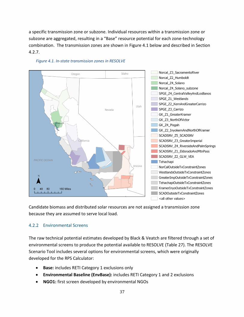
37
a specific transmission zone or subzone. Individual resources within a transmission zone or
subzone are aggregated, resulting in a “Base” resource potential for each zone-technology
combination. The transmission zones are shown in Figure 4.1 below and described in Section
4.2.7.
Figure 4.1. In-state transmission zones in RESOLVE
Candidate biomass and distributed solar resources are not assigned a transmission zone
because they are assumed to serve local load.
Environmental Screens
The raw technical potential estimates developed by Black & Veatch are filtered through a set of
environmental screens to produce the potential available to RESOLVE (Table 27). The RESOLVE
Scenario Tool includes several options for environmental screens, which were originally
developed for the RPS Calculator:
• Base: includes RETI Category 1 exclusions only
• Environmental Baseline (EnvBase): includes RETI Category 1 and 2 exclusions
• NGO1: first screen developed by environmental NGOs

38
• NGO1&2: second screen developed by environmental NGOs
• DRECP/SJV: includes RETI Categories 1 and 2 plus preferred development areas only in
the DRECP (Desert Renewable Energy Conservation Plan)21 and San Joaquin Valley (SJV) .
DRECP/SJV is the default screen for the 2019-2020 IRP.
• Conservative: the potential when all the above screens are applied simultaneously
A more detailed explanation of each environmental screen is available in the Black & Veatch,
RPS Calculator V6.3 Data Updates.22
In the 2017-2018 IRP, candidate solar capacity as calculated from Black and Veatch geospatial
analysis was discounted by 95% to reflect land use constraints and preference for geographic
diversity. This value has been updated to 80% in the 2019-2020 IRP because geographic
diversity is largely enforced by transmission limits. As a result, the solar potential reflected in
Table 27 is four times the 2017-2018 IRP values for most solar resources.
Adjustments are made to the supply curve potentials for certain resources under all
environmental screens. As described in Section 3.2.2.1, a small amount (6,116 MW by 2030) of
the in-state solar is assumed to be developed by California entities outside of CAISO to meet
incremental RPS needs and is therefore made be unavailable to CAISO LSEs for development. In
addition, planned resources with an online date after December 31, 2018 that are included in
the baseline are subtracted from the available potential in the supply curve. Finally, reflecting
commercial interest and recent CAISO interconnection queue capacity, 866 MW of Northern
California wind resources are assumed available under all screens.
Table 27. California renewable potential under various environmental screens
Resource Type Resource Base Env Base NGO1 NGO1&2 DRECP/ SJV Conservative
Biomass InState_Biomass 1,147 1,147 1,147 1,147 1,147 1,147
Geothermal Greater_Imperial 1,352 1,352 1,352 1,352 1,352 1,352
Inyokern_North_Kramer 24 24 24 24 24 24
Northern_California_Ex 469 469 469 469 469 469
Riverside_Palm_Springs 32 32 32 32 32 32
Solano 135 135 135 135 135 135
Geothermal, subtotal 2,012 2,012 2,012 2,012 2,012 2,012
21 https://www.drecp.org/ 22 http://www.cpuc.ca.gov/uploadedFiles/CPUC_Website/Content/Utilities_and_Industries/Energy/Energy_Programs/Electric_Power_Procurement_and_Generation/LTPP/RPSCalc_CostPotentialUpdate_2016.pdf

39
Solar Carrizo 12,021 9,842 11,939 5,867 9,907 5,867
Central_Valley_North_Los_Banos 28,170 19,759 27,707 16,651 12,873 11,801
Distributed 36,605 36,605 36,605 36,605 36,605 36,605
Mountain_Pass_El_Dorado 1,152 60 1,152 41 248 41
Greater_Imperial 27,759 18,632 27,366 17,714 35,216 14,455
Inyokern_North_Kramer 5,211 2,318 5,209 2,265 21,168 1,524
Kern_Greater_Carrizo 20,041 18,280 18,732 12,847 8,329 8,329
Kramer_Inyokern_Ex 8,484 6,138 8,409 6,134 4,508 4,508
North_Victor 6,992 5,886 6,949 5,779 4,608 4,256
Northern_California_Ex 68,912 41,306 67,698 33,367 41,532 33,367
Riverside_Palm_Springs 11,777 5,711 11,757 5,396 57,071 5,396
Sacramento_River 28,684 23,260 27,346 19,784 23,484 19,784
SCADSNV 10,224 3,121 10,122 3,076 5,608 2,162
Solano 16,588 11,937 15,521 9,724 12,025 9,724
Solano_subzone - 4 - 4 - -
Southern_California_Desert_Ex 6,290 3,067 6,230 2,944 43,713 566
Tehachapi_Ex 2,202 1,487 2,168 1,481 1,488 1,481
Tehachapi 17,650 13,480 17,363 13,294 3,801 3,801
Westlands_Ex_Solar 5,358 4,394 5,304 4,269 4,404 4,269
Westlands_Solar 26,671 24,705 26,305 22,599 56,151 22,599
Solar, subtotal 340,791 249,992 333,882 219,841 382,739 190,535
Wind Carrizo 288 288 288 244 287 244
Central_Valley_North_Los_Banos 398 173 352 91 173 91
Distributed - - - - - -
Greater_Imperial 785 - 782 - - -
Greater_Kramer 445 80 389 80 - -
Humboldt 34 34 34 34 34 34
Kern_Greater_Carrizo 69 60 69 60 60 60
Kramer_Inyokern_Ex 81 - 77 - - -
Northern_California_Ex 866 866 866 866 866 866
SCADSNV 100 - 96 - - -
Solano_subzone 50 18 46 1 18 1
Solano 576 550 524 453 542 445
Southern_California_Desert_Ex 48 48 48 48 - -
Tehachapi 802 583 791 572 275 273
Westlands_Ex - - - - - -
Wind, subtotal 4,542 2,700 4,362 2,449 2,255 2,014

40
Out of State Resource Potential
The available potential for out-of-state resources relies primarily on Black & Veatch’s
assessment of renewable resource potential that identifies “high-quality” resources in Western
Renewable Energy Zones (WREZs). WREZ resource potential is aggregated into regional bundles
to create candidate out-of-state renewable resources for RESOLVE. Some of these resources
are assumed to require investments in new transmission to deliver to California loads. These
estimates of resource potential are supplemented with assumptions regarding the availability
of lower capacity factor renewables that may be interconnected on the existing transmission
system.
To explore different levels of out-of-state resource availability, the 2019-2020 IRP cycle includes
four “screens” for out-of-state resources23:
• None: no candidate out-of-state resources are included except for Baja California wind
and Southern Nevada wind and solar resources that directly connect to the CAISO
transmission system.
• Existing Tx Only: only resources that can be interconnected on the existing transmission
system and delivered to California are included as candidate resources.
• Existing & NM/WY wind: New Mexico and Wyoming out-of-state wind resources
requiring major investments in new transmission, are included as candidate resources.
• Existing & New Tx: all out-of-state resources, including those requiring major
investments in new transmission, are included as candidate resources.
The amount of renewable potential included under each screen is summarized in Table 28. All
estimates of potential shown in this table—with the exception of resources assumed to
interconnect to the existing transmission system—are based on Black & Veatch’s potential
assessment. The Existing & NM/WY wind screen is the default screen for the 2019 IRP, however
the default potential of out-of-state wind is limited to 3,000 MW (1,500 MW of Wyoming and
1,500 MW of New Mexico wind resources) to reflect the likelihood that at least one large high-
voltage transmission line (~1,500 MW) to each of these wind resources could be built.
Reflecting commercial interest and recent CAISO interconnection queue capacity, 600 MW of
Baja California wind resources are available for selection in all model runs.
23 Information regarding individual land use screens is available in the Renewable Energy Transmission Initiative 2.0 Plenary Report. https://www.energy.ca.gov/reti/reti2/documents/index.html

41
Table 28. Out-of-state renewable potential under various scenario settings
Type Resource Renewable Potential (MW)
None Existing Tx
Only
Existing &
NM/WY wind
Existing & New
Tx
Geothermal Pacific
Northwest
— — 832
Southern
Nevada
320 320 320 320
Subtotal,
Geothermal
— — — 1,152
Solar Arizona — — — 77,080
New Mexico — — — 664
Southern
Nevada
148,600 148,600 148,600 148,600
Utah — — — 57,656
Subtotal, Solar 148,600 148,600 148,600 284,000
Wind Arizona — — — 2,900
Baja California 600 600 600 600
Idaho — — — 6,869
New Mexico
(Existing Tx)
— 500 500 500
New Mexico
— — 34,580 (Full)
1,500
(Limited)
34,580
Pacific
Northwest
(Existing Tx)
— 1,500 1,500 1,500
Pacific
Northwest
— — — 11,072
Southern
Nevada
442 442 442 442
Utah — — — 5,033
Wyoming
— — 33,862 (Full)
1,500
(Limited)
33,862
Subtotal, Wind 1,042 3,042 71,484 (Full) 97,358

42
Offshore Wind Resource Potential
Data for offshore wind potential is sourced from the UC Berkeley study California Offshore
Wind: Workforce Impacts and Grid Integration.24 The report identifies offshore wind resource
zones based on existing BOEM call areas for California, as well as potential future development
sites identified in studies by BOEM and NREL. Resources in the Morro Bay, Diablo Canyon,
Humboldt Bay, Cape Mendocino, and Del Norte zones are included in the 2019-2020 IRP. The
offshore wind resource potential assumptions are shown below.
Table 29. Offshore Wind Resource Potential
Offshore Wind Resource Zone Resource Potential Area (Sq. km) Resource Potential (MW)
Del Norte 2,201 6,604
Cape Mendocino 2,072 6,216
Diablo Canyon 1,441 4,324
Morro Bay 806 2,419
Humboldt Bay 536 1,607
Total 7,051 21,171
Note that the offshore resource potential shown in Table 29 represents that amount that could
be developed offshore. Onshore transmission limitations in RESOLVE described in section 4.2.7
effectively reduce the available resource significantly, especially for the remote Northern
California resources (Humboldt Bay, Cape Mendocino, and Del Norte).
First Available Year and Annual Deployment Limits
Assumptions for the first available year of candidate renewables resource types in the 2019-
2020 IRP cycle reflect feasible timelines for bring resources online based on the current
interconnection queue and typical development timelines. The first available year in RESOLVE is
applied on a resource-by-resource basis; accordingly, a range of years applies when
summarizing by resource type in Table 30.
24 Available at: http://laborcenter.berkeley.edu/offshore-wind-workforce-grid/

43
Table 30. First available year by candidate renewable resource type
Resource Type First Available Year
Solar PV 2020
Wind (CA onshore) 2022-2023
Wind (OOS onshore) 2026
Wind (offshore) 2030
Geothermal 2024-2026
Biomass 2020
Pumped Storage 2026
Battery Storage 2020
In addition to limiting the deployment of resources based on the first available year, RESOLVE
can also enforce annual deployment limits over a group of resources. The 2019-2020 IRP
includes the option to limit the sum of candidate utility-scale and candidate distributed solar
resource selection to 2 GW/yr from 2020 through 2023. Historical levels of utility-scale solar
development in CAISO and California inform the choice of the 2 GW/yr value. Growth in
baseline BTM and utility-scale solar capacity is not included under the 2 GW/yr limit.
Resource Cost
NREL’s 2018 Annual Technology Baseline is used as the primary basis for renewable generation
cost updates.25 The assumptions for RESOLVE renewable resources are shown in the tables
below for in-state, out-of-state, and offshore wind resources, respectively. The input to
RESOLVE is an assumed levelized fixed cost ($/kW-yr) for each resource; this is translated into
the levelized cost of energy ($/MWh) for comparability with typical Power Purchase
Agreements (PPA) entered into between LSEs and third-party developers.
25 Biomass capital costs were revised from Annual Technology Baseline assumptions based on stakeholder input

44
Table 31. California renewable resource cost & performance assumptions
Capital Cost (2016 $/kW) Implied Levelized Cost of Energy
(2016 $/MWh)
Resource Capacity
Factor 2020 2022 2026 2030 2020 2022 2026 2030
Biomasss InState_Biomass 85% $4,138 $4,063 $3,997 $3,941 $115 $114 $117 $118
Geothermal
Greater_Imperial_Geothermal 88% $5,212 $5,186 $5,133 $5,080 $83 $83 $91 $94
Inyokern_North_Kramer_Geothermal 80% $5,212 $5,186 $5,133 $5,080 $91 $91 $101 $103
Northern_California_Ex_Geothermal 81% $5,212 $5,186 $5,133 $5,080 $90 $90 $99 $102
Riverside_Palm_Springs_Geothermal 80% $5,212 $5,186 $5,133 $5,080 $91 $91 $101 $103
Solano_Geothermal 90% $5,212 $5,186 $5,133 $5,080 $81 $81 $89 $92
Solar (solar capital
costs shown in $/kW-
ac)
Carrizo_Solar 32% $1,334 $1,250 $1,193 $1,136 $28 $26 $30 $29
Central_Valley_North_Los_Banos_Solar 30% $1,334 $1,250 $1,193 $1,136 $30 $28 $33 $32
Distributed_Solar 23% $2,201 $2,040 $1,779 $1,517 $59 $54 $59 $52
Greater_Imperial_Solar 34% $1,334 $1,250 $1,193 $1,136 $26 $24 $29 $28
Inyokern_North_Kramer_Solar 36% $1,334 $1,250 $1,193 $1,136 $25 $23 $27 $26
Kern_Greater_Carrizo_Solar 31% $1,334 $1,250 $1,193 $1,136 $29 $27 $31 $30
Kramer_Inyokern_Ex_Solar 36% $1,334 $1,250 $1,193 $1,136 $25 $23 $27 $26
North_Victor_Solar 36% $1,334 $1,250 $1,193 $1,136 $25 $23 $27 $26
Northern_California_Ex_Solar 30% $1,334 $1,250 $1,193 $1,136 $30 $27 $32 $31
Riverside_Palm_Springs_Solar 34% $1,334 $1,250 $1,193 $1,136 $26 $24 $28 $28
Sacramento_River_Solar 29% $1,334 $1,250 $1,193 $1,136 $31 $28 $33 $32
SCADSNV_Solar 34% $1,334 $1,250 $1,193 $1,136 $26 $24 $29 $28
Solano_Solar 29% $1,334 $1,250 $1,193 $1,136 $31 $28 $33 $32
Solano_subzone_Solar 28% $1,334 $1,250 $1,193 $1,136 $32 $30 $35 $34
Southern_California_Desert_Ex_Solar 35% $1,334 $1,250 $1,193 $1,136 $26 $24 $28 $27
Tehachapi_Ex_Solar 31% $1,334 $1,250 $1,193 $1,136 $29 $26 $31 $30

45
Tehachapi_Solar 35% $1,334 $1,250 $1,193 $1,136 $25 $23 $28 $27
Westlands_Ex_Solar 32% $1,334 $1,250 $1,193 $1,136 $28 $26 $30 $29
Westlands_Solar 30% $1,334 $1,250 $1,193 $1,136 $29 $27 $32 $31
Wind
Carrizo_Wind 30% $1,693 $1,692 $1,692 $1,694 $50 $55 $63 $63
Central_Valley_North_Los_Banos_Wind 30% $1,693 $1,692 $1,692 $1,694 $50 $56 $63 $63
Greater_Imperial_Wind 35% $1,615 $1,602 $1,580 $1,563 $39 $45 $52 $52
Greater_Kramer_Wind 31% $1,681 $1,678 $1,674 $1,674 $48 $53 $61 $61
Humboldt_Wind 33% $1,624 $1,612 $1,593 $1,580 $42 $47 $54 $54
Kern_Greater_Carrizo_Wind 28% $1,693 $1,692 $1,692 $1,694 $54 $59 $66 $66
Kramer_Inyokern_Ex_Wind 29% $1,693 $1,692 $1,692 $1,694 $53 $58 $65 $66
Northern_California_Ex_Wind 30% $1,687 $1,685 $1,683 $1,683 $49 $54 $61 $62
SCADSNV_Wind 31% $1,647 $1,639 $1,626 $1,618 $46 $52 $59 $59
Solano_subzone_Wind 32% $1,693 $1,692 $1,692 $1,694 $46 $52 $59 $59
Solano_Wind 30% $1,685 $1,683 $1,680 $1,680 $49 $54 $61 $62
Southern_California_Desert_Ex_Wind 27% $1,693 $1,692 $1,692 $1,694 $57 $62 $69 $69
Tehachapi_Wind 33% $1,634 $1,624 $1,607 $1,596 $42 $47 $55 $54

46
Table 32. Out-of-state renewable resource cost & performance assumptions. Costs in this table do not include the incremental cost of new, long
distance transmission lines.
Capital Cost (2016 $/kW) Implied Levelized Cost of Energy
(2016 $/MWh)
Resource Capacity Factor 2020 2022 2026 2030 2020 2022 2026 2030
Pacific_Northwest_Geothermal 84% $5,109 $5,083 $5,031 $4,980 $85 $85 $94 $96
Southern_Nevada_Geothermal* 80% $5,056 $5,031 $4,980 $4,929 $88 $89 $98 $100
Arizona_Solar 34% $1,291 $1,210 $1,155 $1,100 $26 $24 $28 $27
New_Mexico_Solar 33% $1,273 $1,193 $1,138 $1,084 $26 $24 $28 $27
Utah_Solar 30% $1,281 $1,201 $1,146 $1,091 $29 $26 $31 $30
Southern_Nevada_Solar* 32% $1,296 $1,215 $1,159 $1,104 $27 $25 $30 $29
Arizona_Wind 29% $1,657 $1,656 $1,655 $1,658 $50 $55 $62 $63
Baja_California_Wind* 36% $1,583 $1,574 $1,558 $1,547 $37 $42 $49 $49
Idaho_Wind 32% $1,630 $1,627 $1,623 $1,622 $45 $50 $57 $57
New_Mexico_Wind 44% $1,472 $1,442 $1,388 $1,345 $27 $33 $39 $38
NW_Ext_Tx_Wind 30% $1,695 $1,694 $1,694 $1,696 $50 $55 $62 $63
Pacific_Northwest_Wind 32% $1,654 $1,649 $1,641 $1,637 $45 $51 $58 $58
SW_Ext_Tx_Wind 36% $1,576 $1,565 $1,547 $1,533 $36 $41 $48 $48
Utah_Wind 31% $1,629 $1,625 $1,619 $1,617 $47 $52 $59 $59
Wyoming_Wind 44% $1,476 $1,443 $1,387 $1,340 $27 $32 $39 $38
Southern_Nevada_Wind* 28% $1,660 $1,659 $1,659 $1,661 $54 $59 $66 $66
*Assumed to directly interconnect to the CAISO system

47
Table 33. Offshore wind resource cost & performance assumptions. Only 2030 costs are used in RESOLVE because offshore wind is available for
selection starting in 2030.
Capital Cost (2016 $/kW) Implied Levelized Cost of Energy
(2016 $/MWh)
Resource Capacity Factor 2020 2022 2026 2030 2020 2022 2026 2030
Humboldt_Bay_Offshore_Wind 52% $5,058 $4,707 $4,086 $3,559 $80 $83 $88 $76
Morro_Bay_Offshore_Wind 55% $5,058 $4,707 $4,086 $3,559 $75 $77 $81 $71
Diablo_Canyon_Offshore_Wind 46% $5,353 $4,988 $4,343 $3,794 $94 $97 $103 $90
Cape_Mendocino_Offshore_Wind 53% $5,058 $4,707 $4,086 $3,559 $78 $81 $85 $74
Del_Norte_Offshore_Wind 52% $5,058 $4,707 $4,086 $3,559 $80 $83 $88 $76

48
4.2.6.1 Solar Capital Cost Assumptions
The NREL Annual Technology Baseline is used to determine both capital costs and operating
costs of solar PV resources for each forecast year. Both utility-scale and distributed solar PV
cost projections use Annual Technology Baseline data.
Three capital cost trajectories are developed based on the Annual Technology Baseline. The
“Low” case follows a more ambitious trajectory fueled by increased R&D funding,
improvements in technology, and/or aggressive global demand, while the “Mid” case
represents a medium level scenario. The “High” case assumes no improvements beyond
present-day cost levels. The impact of tariffs on PV modules is not part of the 2018 Annual
Technology Baseline’s base capital costs but is included as a capital cost adder in certain
scenarios that could be utilized in the 2019-2020 IRP process.
Table 34. Cost trajectories for solar PV (% of 2016 capital cost)
RESOLVE Scenario Setting 2020 2022 2026 2030
Low 48% 45% 39% 34%
Mid 54% 41% 49% 44%
High 65% 66% 66% 66%
The Annual Technology Baseline’s solar cost data is location-independent (developed to be free
of geographical factors) and regional adjustments are made to reflect California and out-of-
state conditions, if material. Consistent with current industry practice, cost calculations assume
a single-axis tracking system with a 1.35 inverter loading ratio for utility-scale solar and a fixed-
tilt system with 1.1 inverter loading ratio for distributed solar. The inverter loading ratio
measures the amount of DC solar cells per the inverters rated AC output. For example, a 10
MW-AC inverter would typically be used for a solar system with 13.5 MW-DC of photovoltaics.
Solar O&M is estimated based on an average ratio of O&M to capital expenditure (CAPEX)
reported in the Annual Technology Baseline. This treatment implicitly assumes that the same
historical correlations seen in O&M and CAPEX cost reductions will hold into the future.
4.2.6.2 Wind Capital Cost Assumptions
NREL’s 2018 Annual Technology Baseline also provides estimates of onshore wind costs. The
Annual Technology Baseline develops regional sets of CAPEX values for a full range of observed
wind speeds, resulting in a total of 10 bins, or “techno-resource groups” (TRGs). Zones with
lower wind speeds are assumed to employ higher rotors to compensate, and therefore

49
correspond to a higher CAPEX per MW of installed capacity. TRGs that resemble California and
out-of-state wind conditions are used in the 2019-2020 IRP cycle. As for solar, the Annual
Technology Baseline provides base CAPEX and O&M values for wind, as well as three cost
trajectories: Low, Mid, and Constant. The Annual Technology Baseline’s estimates of the O&M
of wind do not include regional variants and are assumed to be the same at all locations. NREL
notes significant uncertainty in its estimation of wind O&M costs, largely due to limited publicly
available data and the tendency for wind O&M to vary significantly by project due to vintage,
capacity, location.
Table 35. Cost trajectories for wind26 (% of 2016 capital cost)
RESOLVE Scenario Setting 2020 2022 2026 2030
Low 94% 86% 68% 51%
Mid 98% 98% 97% 96%
High 103% 103% 103% 103%
CAISO Transmission Cost & Availability
Candidate renewable resources in RESOLVE are selected as fully deliverable (Full Capacity
Deliverability Status, or FCDS) resources or energy only (Energy Only Deliverability Status, or
EO) resources, each representing a different classification of deliverability status by CAISO. A
resource with FCDS is included in RESOLVE’s resource adequacy constraint and is counted
towards system resource adequacy, as described in Section 7.1. An EO resource is excluded
from RESOLVE’s resource adequacy constraint, thereby not providing any resource adequacy
value. The FCDS or EO status of a resource does not impact how it is represented in RESOLVE’s
operational module – the total installed capacity of the resource is used when simulating hourly
system operations, regardless of FCDS or EO designation.
In each transmission zone, RESOLVE selects resources in three categories:
• FCDS resources on the existing system. Each transmission zone is characterized by the
amount of new resource capacity that can be installed on the existing system while still
receiving full capacity deliverability status. Renewables within each transmission zone
compete with one another for existing, zero marginal cost FCDS transmission capacity.
26 Shown for TRG 6 (36% capacity factor). Lower TRGs have steeper cost declines trajectories, while higher TRGs have slower declines.

50
RESOLVE will typically prioritize FCDS for resources with a higher resource adequacy
contribution.
• EO resources on the existing system. Each transmission zone is also characterized by
the amount of incremental energy-only capacity that can be installed beyond the FCDS
limits (i.e. this quantity is additive to the FCDS limit). For each renewable resource,
RESOLVE can choose for it to have EO status on the existing transmission system if EO
capacity is available. In this case, the renewable resource does not contribute to the
planning reserve margin.
• FCDS resources on new transmission. Resources in excess of the limits of the existing
system may be installed but require investment in new transmission. This may occur (1)
if both the FCDS and EO limits are reached; or (2) if the FCDS limit is reached and the
value of new capacity exceeds the cost of the new transmission investment.
Figure 4.2. Conceptual diagram of transmission costs and capacity for candidate renewable resources
in RESOLVE
RESOLVE does not currently include the option to upgrade the transmission system to increase
the energy only capacity of a transmission zone.
Candidate distributed solar and wind resources are assumed to be fully deliverable on the
existing transmission system and do not incur additional transmission costs. These resources
are assigned a transmission zone of “None.”

51
CAISO has produced transmission capability and cost estimates for use in IRP modeling.27
CAISO’s whitepaper includes a table with a list of electrical zones, transmission capability
estimates of the existing transmission system, and the cost and capacity of potential upgrades.
CAISO’s estimates are adjusted for use in RESOLVE (Table 37) by:
• Subtraction of baseline resource capacity that is projected to come online in 2019 or
later from CAISO’s transmission capability estimates. Resources brought online after
2018 must be allocated incremental transmission capacity because CAISO’s transmission
capability values include all resources online at the end of 2018.
• Conversion of upgrade cost and upgrade capacity into levelized, $/kW-yr values that are
consistent with the “nested” transmission constraint formulation in RESOLVE (described
below). RESOLVE does not impose limitations on the size of new transmission
investments.
In the whitepaper CAISO identifies multiple layers of transmission constraints for many
transmission zones. These “nested” constraints represent multiple concurrent limitations to
delivering energy from renewable resource zones to load centers (Figure 4.3). While only one
limit may be binding at a time, all limits must be modeled simultaneously to ensure that no
limits are exceeded. In RESOLVE, nested constraints are modeled by allowing candidate
resources to be assigned to multiple (nested) transmission zones. By allowing multiple
assignments, a candidate resource counts towards the FCDS and EO limits in all of the zones ad
subzones to which it is assigned.
27 http://www.caiso.com/Documents/TransmissionCapabilityEstimates-Inputs-CPUCIntegratedResourcePlanPortfolioDevelopment-Call052819.html

52
Figure 4.3. Diagram of nested transmission constraints
Transmission upgrade costs from the CAISO whitepaper are implemented in RESOLVE using the
incremental cost to upgrade transmission from inner nested zone to the next outer nest,
thereby creating a “layer cake” of transmission upgrade costs to get to the wider CAISO
transmission system. For example, in Figure 4.3, resources R1 and R2 contribute to the existing
FCDS capability limit (or energy only limit) for both Zone 1 and Zone 2. Resource R3 only
contributes to the corresponding limits for Zone 1. Selecting resources R1 and R2 may trigger an
upgrade (illustrated with a yellow arrow pointing from Zone 2 to Zone 1) to increase
deliverability into the next constrained layer (Zone 1). Separately, all three resources may
trigger a transmission upgrade to ensure deliverability out of Zone 1 into the rest of the CAISO
system (the red arrow pointing out of Zone 1). If it is necessary to upgrade both transmission
lines (yellow and red arrows) to deliver capacity from R1 or R2 to the rest of the CAISO system,
the sum of the cost to build capacity along the yellow and red arrows is incurred.
Table 37 includes the incremental cost to build new FCDS transmission. For subzones that are
within another zone, this is the cost to build transmission to the next zone level (from right to
left on Table 36). For zones that are an outermost transmission zone, the incremental cost is
equal to the total cost to build new FCDS transmission because only one upgrade is required to
reach load centers. For zones that are not an outermost transmission zone, transmission costs
may be incurred at multiple levels of transmission zones. The nested zone formulation also
applies for FCDS and EO availability on existing transmission in Table 36 – for resources that are
in a subzone, transmission capacity must also be reserved in all outer zones.

53
Table 36. RESOLVE transmission zone “nested” hierarchy
Outermost Transmission Zone Subzone Level 1 Subzone Level 2 (Innermost)
Southern CA Desert and Southern
Nevada
(SCADSNV)
Mountain_Pass_El_Dorado
(Eldorado/Mtn Pass) -
GLW_VEA (Southern Nevada) -
Greater_Imperial (Greater Imperial)* -
Riverside_Palm_Springs (Riverside
East & Palm Springs)* -
SPGE (Southern PG&E)**
Kern_Greater_Carrizo (Kern and
Greater Carrizo) Carrizo (Carrizo)
Central_Valley_North_Los_Bano
s (Central Valley North & Los Banos) -
Greater_Kramer (Greater Kramer (North
of Lugo))*** North_Victor (North of Victor)
Inyokern_North_Krame
r (Inyokern and North of
Kramer)
Sacramento_River (Northern
CA/Sacramento River)
Solano (Solano) Solano Subzone
(Solano_subzone)
Humboldt (Humboldt) -
Tehachapi (Tehachapi) - -
Kramer_Inyokern_Ex
“_Ex” zones have available transmission capacity- indicated by active capacity in
CAISO’s interconnection queue- but are outside of CAISO’s defined transmission
zones. The “_Ex” zones do not have subzones in RESOLVE.
Northern_California_Ex
Southern_California_Desert_Ex
Tehachapi_Ex
Westlands_Ex
OffshoreWind_UnknownCost
CAISO's Whitepaper does not identify transmission upgrades that would be
able to deliver offshore wind (or other candidate resource) capacity from the
Northern California coast to demand centers. This zone is included for offshore
wind resources with unknown cost to develop onshore transmission. A
limitingly high upgrade cost is assumed due to lack of data. This zone does not
have any subzones.
None
The “None” zone bypasses transmission zone limitations, giving resources in
this “zone” unlimited fully deliverable transmission. Only appropriate for
distributed resources, and/or resources that serve local load. This zone does
not have any subzones.

54
CAISO zone or sub-zone name shown in parentheses. Notes:
* CAISO identifies overlap between the Greater Imperial and Riverside East & Palm Springs transmission
zones. RESOLVE models resources in this overlapping area within Greater Imperial but not Riverside East
& Palm Springs because transmission availability of the Greater Imperial zone is more limiting.
** To adapt CAISO transmission constraint data into a format that is compatible with the RESOLVE
nested constraint formulation, The Westlands subzone identified by CAISO is split between two zones in
RESOLVE: 1) Kern and Greater Carrizo and 2) Central Valley North & Los Banos. The Westlands_Ex zone
is used for resource capacity outside of the geographical extent of CAISO’s Westlands zone.
*** Pisgah zone not modeled in RESOLVE due to a lack of candidate resources.

55
Table 37. Transmission availability & cost in CAISO
Transmission Zone or Subzone
Incremental
Deliverability Cost
($/kW-yr)
FCDS Availability on
Existing Transmission,
Net of Post-2018 COD
Baseline Capacity
(MW)
Energy-Only
Availability on
Existing Transmission
(MW)***
Carrizo $10 187 0
Central_Valley_North_Los_Banos $36 791 0
GLW_VEA $14 596 0
Greater_Imperial $221 919 1900
Greater_Kramer $48 597 0
Humboldt $999** 0 100
Inyokern_North_Kramer $161 97 0
Kern_Greater_Carrizo $21 784 700
Kramer_Inyokern_Ex* $48 860 0
Mountain_Pass_El_Dorado $7 250 2150
None $0 0 0
North_Victor $161 300 0
Northern_California_Ex* $19 866 0
Riverside_Palm_Springs $88 2665 2550
OffshoreWind_UnknownCost $999** 0 0
Sacramento_River $19 1995 2600
SCADSNV $102 2434 6600
Solano $21 599 700
Solano_subzone $999** 0 0
Southern_California_Desert_Ex* $102 862 0
SPGE $7 675 700
Tehachapi $13 3677 800
Tehachapi_Ex* $13 1870 0
Westlands_Ex* $7 1779 0
* Resources that end in “Ex” refers to areas outside of the CAISO transmission cost and availability estimates
** $/999 kW-yr indicates that the upgrade cost is unknown, so an extremely high value is placed on transmission
upgrades.
*** Zero is assumed for zones where Estimated EO Capability is noted as “TBD” in CAISO’s whitepaper, except for
the Kern_Greater_Carrizo subzone (and SPGE zone), which include 700 MW of EO capability from CAISO’s “Tx
Capability Estimates for 2019-2020 TPP
Out-of-State Transmission Cost
New out-of-state resources delivered to the CAISO system are attributed an additional
transmission cost, representing either the cost to wheel power across adjacent utilities’ electric

56
systems (for resources delivered on existing transmission) or the cost of developing a new
transmission line (for resources delivered on new transmission). Wheeling costs on the existing
system are derived from utilities’ Open Access Transmission Tariffs; the cost of new
transmission lines are based on assumptions developed for the CEC’s Renewable Energy
Transmission Initiative 2.0 (RETI 2.0).28
Table 38. Transmission costs for out-of-state resources
Zone Existing Transmission
Cost ($/kW-yr)
New Transmission Cost
($/kW-yr)
Arizona — $29
Idaho — $129
New Mexico $72 $121
Northwest $34 $99
Utah — $69
Wyoming — $125
Resources that require new transmission to reach the CAISO system are assumed to be
delivered to a specific CAISO transmission zone or subzone. Each out-of-state resource must
compete for CAISO transmission capacity with other candidate renewable resources located
inside the CAISO system. The total cost to deliver out-of-state resources on new transmission to
CAISO load centers is the cost shown in Table 38, plus any additional cost to develop
transmission in CAISO transmission zones and/or subzones (Section 4.2.7) if the capacity of the
existing CAISO transmission system is not sufficient.
4.3 Energy Storage
Energy storage cost and performance characteristics can vary significantly by technical
configuration and use case. To flexibly model energy storage systems of differing sizes and
durations, the cost of storage is broken into two components: capacity ($/kW) and duration
($/kWh). The capacity cost refers to all costs that scale with the rated installed power (kW)
while the duration costs refers to all costs that scale with the energy of the storage resource
(kWh). This breakout is intended to capture the different drivers of storage system costs. For
28 https://www.energy.ca.gov/reti/

57
example, a 1 kW battery system would require the same size inverter whether it is a four- or
six-hour battery but would require additional cells in the longer duration case.
For pumped storage, capacity costs are the largest fraction of total costs and relate to the costs
of the turbines, the penstocks, the interconnection, etc., while duration costs are relatively
small and mainly cover the costs of preparing a reservoir. For Lithium Ion (Li-ion) batteries, the
capacity costs mainly relate to the cost of an inverter and other power electronics for the
interconnection, while the duration costs relate to Li-ion battery cells. For flow batteries, the
capacity costs relate to the cost of an inverter and other power electronics, as well as the ion
exchange membrane and fluids pumps, while the duration costs mainly relate to the tanks and
the electrolyte. As a result, the capacity component of flow battery costs is higher than that of
Li-ion, while the duration component is lower.
Pumped Storage
As in the 2017-2018 IRP cycle, the capital costs of candidate pumped storage resources for the
2019-2020 IRP are based on Lazard’s Levelized Cost of Storage 2.0 (2016).29 Pumped storage
costs are assumed to remain constant in real terms. Candidate pumped storage resources must
have at least 12 hours of duration.
Table 39. Pumped storage cost components
Cost Component Capital Cost -
Power ($/kW)
Capital Cost -
Energy ($/kWh)
Fixed O&M Cost
($/kW-yr)
Capital Cost - Power ($/kW) $1,307 $131 $13
These capital costs are fed into a pro forma model to estimate levelized fixed costs, using the
following assumptions:
• Financing lifetime of 50 years
• Fixed O&M of $13/kW-yr with an annual escalation of 2%
• No variable O&M costs
29 Later releases of Lazard do not include pumped storage costs. Available at: https://www.lazard.com/perspective/levelized-cost-of-storage-analysis-20/. E3 used the average of the range provided in p. 31 of the Appendix. For the breakout of power to energy cost, E3 used the specified duration (8-hours) and assumed energy costs per kWh are 1/10th of the power costs per kW.

58
• After-tax WACC of 9.13%.
The resulting all-in levelized fixed costs are shown below.
Table 40. Pumped storage all-in levelized fixed costs.
Cost Component 2020 2022 2026 2030
Levelized Power Cost
($/kW)
$131 $118 $107 $109
Levelized Energy Cost
($/kWh)
$11 $10 $9 $9
The pumped storage resource potential assumptions are shown in the table below.
Table 41. Available potential by year (MW) for candidate pumped storage resources.
Resource Class 2020 2022 2026 2030
Potential (MW) - - 4,000 4,000
Battery Storage
Battery storage costs are attributed to either the capacity or duration category using AC and DC
storage component cost data and comparisons of storage costs at differing durations.30 The
types of costs included in each category are summarized below:
• Capacity (kW): Inverter, switches and breakers, other balance of system and
Engineering, procurement and construction (EPC) costs.
• Duration (kWh): Battery cell modules, racking frame/cabinet, battery management
system.
The total cost of an energy storage system is calculated by summing the cost for each capacity
and duration “building block.” Reflecting the hourly dispatch interval used in RESOLVE,
candidate battery storage resources must have at least 1 hour of duration.
30 Duration costs are considered to include all costs in Lazard’s “Initial capital cost - DC” category, whereas capacity costs include both “Initial capital cost – AC” and “Other Owners Costs.”

59
The 2019-2020 IRP cycle includes both wholesale and Behind-The-Meter (BTM) battery storage
as candidate resources and relies on storage cost assumptions from Lazard’s Levelized Cost of
Storage 4.0 (2018) and supplemented by NREL’s Solar and Storage Report.31, 32 Cost
assumptions for candidate wholesale storage are derived from Lazard’s peaker replacement use
case using the methodology described above. Both Li-ion and Flow technologies are included as
candidate wholesale battery storage resources. While paired battery technologies are not
explicitly modeled in RESOLVE, paired battery storage can be represented with a separate cost
trajectory that includes ITC benefits and other co-location cost savings. Candidate BTM battery
storage is assumed to be Li-ion technology, with costs derived from Lazard’s commercial use
case for Li-ion.
Given the uncertainty regarding future battery costs, the 2019-2020 IRP inputs include low, mid
and high cost options to reflect a range of potential cost trajectories. In addition to breaking out
capital costs between capacity and duration, different O&M costs are attributed to each of
these categories. For example, warranty and augmentation costs are assumed to cover battery
cell performance, thus are attributed to the duration category.
Forecasts for storage cost declines are based on Lazard through 2022, the last year of the
Lazard forecast. After 2022, it is assumed the pace of cost reductions slows to zero at a linear
rate through 2030 (i.e. storage costs flatten out by 2030). Cost reduction factors are applied
equally to capital costs in the capacity and duration categories.
31 Available at: https://www.lazard.com/media/450774/lazards-levelized-cost-of-storage-version-40-vfinal.pdf 32 Available at: https://www.nrel.gov/docs/fy19osti/71714.pdf

60
Table 42. Capital cost assumptions for candidate battery resources
Resource Cost Component Case 2020 2022 2026 2030
Li-Ion
Battery
(Utility-
Scale)
Capital Cost –
Power ($/kW)
Low $177 $147 $107 $88
Mid $191 $162 $122 $105
High $228 $196 $153 $137
Capital Cost –
Energy ($/kWh)
Low $221 $184 $133 $110
Mid $265 $224 $169 $145
High $392 $338 $264 $235
Fixed O&M (%) All 1.5% 1.5% 1.5% 1.5%
Li-Ion
Battery
(Utility-
Scale,
paired)
Capital Cost –
Power ($/kW)
Low $47 $39 $28 $23
Mid $50 $43 $32 $28
High $60 $52 $40 $36
Capital Cost –
Energy ($/kWh)
Low $221 $184 $133 $110
Mid $265 $224 $169 $145
High $392 $338 $264 $235
Fixed O&M (%) All 1.5% 1.5% 1.5% 1.5%
Li-Ion
Battery
(BTM)
Capital Cost –
Power ($/kW)
Low $180 $150 $111 $96
Mid $245 $207 $157 $139
High $300 $259 $202 $180
Capital Cost –
Energy ($/kWh)
Low $382 $318 $234 $204
Mid $546 $462 $350 $309
High $686 $590 $461 $411
Fixed O&M (%) All 3.20% 3.20% 3.20% 3.20%
Flow
Battery
Capital Cost –
Power ($/kW)
Low $611 $545 $452 $415
Mid $1,240 $1,119 $944 $872
High $1,882 $1,717 $1,473 $1,373
Capital Cost –
Energy ($/kWh)
Low $169 $151 $125 $115
Mid $222 $200 $169 $156
High $276 $252 $216 $202
Fixed O&M (%) All 0.80% 0.80% 0.80% 0.80%
Battery capital costs are fed into a pro forma model to estimate levelized fixed costs, using the
following assumptions: financing lifetime of 20 years (10 years for BTM batteries), ITC eligibility,
and after-tax WACC of 9.13%. The resulting all-in levelized fixed costs of the mid case are shown
in Table 43.

61
Table 43. Candidate battery levelized fixed costs - Mid
Resource Cost Component 2020 2022 2026 2030
Li-Ion
Battery
Levelized Fixed Cost
– Power ($/kW-yr) $24 $19 $13 $11
Levelized Fixed Cost
– Energy ($/kWh-yr) $42 $33 $23 $19
Li-Ion
Battery
(Paired)
Levelized Fixed Cost
– Power ($/kW-yr) $5 $4 $3 $3
Levelized Fixed Cost
– Energy ($/kWh-yr) $32 $25 $20 $17
Li-Ion
Battery
(BTM)
Levelized Fixed Cost
– Power ($/kW-yr) $51 $42 $30 $27
Levelized Fixed Cost
– Energy ($/kWh-yr) $131 $106 $76 $66
Flow
Battery
Levelized Fixed Cost
– Power ($/kW-yr) $143 $120 $94 $87
Levelized Fixed Cost
– Energy ($/kWh-yr) $26 $22 $16 $14
RESOLVE does not limit the available potential for candidate battery storage resources.
4.4 Demand Response
Shed Demand Response
Shed (or “conventional”) demand response reduces demand only during peak demand events.
Assumptions on the cost, performance, and potential of candidate new shed demand response
resources are based on Lawrence Berkeley National Laboratory’s report for the CPUC: Final
Report on Phase 2 Results: 2025 California Demand Response Potential Study.33 The resource
potential supply curve is based on data outputs from LBNL’s DRPATH model, with the scenario
assumptions outlined below in Table 44. DRPATH potential estimates are not incremental to
existing demand response programs. Consequently, LSE demand response programs, including
demand response procured through DRAM, are removed from the DRPATH supply curve
because these programs are represented as baseline resources (see Section 3.5). On the
assumption that lower cost DR has been the focus of LSE DR programs, DR potential is removed
33 Lawrence Berkeley National Laboratory, Final Report on Phase 2 Results: 2025 California Demand Response Potential Study (2017). Available at: http://www.cpuc.ca.gov/General.aspx?id=10622

62
from the supply curve in order of least to most expensive (Figure 4.4Error! Reference source
not found.). To reflect the lead time that would be required to ramp up shed DR availability, the
potential of each tranche of the Shed DR supply curve is phased in linearly between 2020 and
2025. Sensitivity analysis explores resource portfolio selection when all shed DR potential is
available in all modeled years.
Table 44. Scenario assumptions for LBNL’s DRPATH model used to generate shed DR supply curve data
for IRP modeling
Category Assumption
Base year 2020
DR Availability
Scenario
Medium
Weather 1 in 2 weather year
Energy
Efficiency
Scenario
Mid AAEE
Rate Scenario Rate Mix 1—TOU and CPP (as defined by
LBNL report)
Cost
Framework
Gross
Figure 4.4. Conventional Demand Response Supply Curve
Shift Demand Response
“Shift” demand response (also called “flexible load”) in RESOLVE is an energy-neutral resource
that can move demand within a day, subject to hourly and daily constraints on the amount of
-
200
400
600
800
1,000
1,200
$25 $50 $75 $100 $125 $150 $175 $200
Pea
k Lo
ad Im
pact
Annualized Cost ($/kW-yr)
Conventional DR supply curve
Remaining Potential in Supply Curve
Baseline

63
energy that can be shifted. End-use energy consumption in RESOLVE can be shifted, for
example, from on-peak hours to off-peak hours; the maximum amount of energy shifted in one
day is the daily energy budget. The quantity of shift demand response is reported in units of
(MWh/day)-yr, which is the average available daily energy budget for a given year. RESOLVE
includes a constraint that sets a maximum quantity of energy that can be shifted in one hour. It
is currently assumed that the full daily energy budget is available on every day of the year. It is
also assumed that there is no efficiency loss penalty incurred by shifting loads to other times of
the day.
Assumptions on the cost, performance, and potential of candidate advanced demand response
resources are based on Lawrence Berkeley National Laboratory’s report for the CPUC: Final
Report on Phase 2 Results: 2025 California Demand Response Potential Study.34 The resource
potential supply curve is based on data outputs from LBNL’s DRPATH model, with the same set
of scenario assumptions used to create the Shed DR supply curve (see Table 44).
Figure 4.5. Shift demand response: total annual costs vs potential daily energy budget
The 2019 IRP does not include a scenario in which shift DR is available for selection as a
candidate resource.
34 Lawrence Berkeley National Laboratory, Final Report on Phase 2 Results: 2025 California Demand Response
Potential Study (2017). Available at: http://www.cpuc.ca.gov/General.aspx?id=10622

64
5. Pro Forma Financial Model
This section describes the purpose of and methodology behind the pro forma financial model.
The pro forma model is a discounted cash flow model used to calculate the levelized costs of
different candidate resources. The primary outputs from the model are the levelized fixed costs
for each resource. Levelized fixed costs calculated by the pro forma include the overnight
capital cost for each resource, financing costs (including investor returns on a project), fixed
O&M costs, and any capital-based tax credits, such as the Investment Tax Credit (ITC) and the
Production Tax Credit (PTC), which are used to offset capital costs.
The pro forma used for the 2019-2020 IRP assumes financing is provided by an Independent
Power Producer (IPP), which reflects current development practices in which most new
resources in California are third-party owned and contracted with LSEs rather than financed by
LSEs themselves. Financing assumptions assumed in the pro forma model are based on NREL’s
2018 Annual Technology Baseline.35
Levelized costs are calculated in the pro forma using real levelization to yield costs that are flat
in real dollar terms. This approach discounts annual project costs using a nominal discount rate
(nominal return on equity) and discounts energy and capacity using a real discount rate (real
return on equity). This is a standard approach that yields levelized costs in flat real terms for
input to the RESOLVE model.
The pro forma also requires information on variable costs (such as fuel and variable O&M) and
resource performance characteristics. These inputs are considered in the pro forma financing
optimization but have minimal impacts on levelized fixed costs. In addition, variable costs
included in the pro forma model do not directly flow through to RESOLVE as inputs in the
modeling process.
35 Financing assumptions include WACC, cost of debt and debt fraction. E3 adjusted NREL’s cost of debt to reflect the current rate environment. based on the spread to the Industrial Baa bond rate, as used by EIA in the Annual Energy Outlook.

65
6. Operating Assumptions
6.1 Overview
RESOLVE’s objective function includes the annual cost to operate the electric system across
RESOLVE’s footprint; this cost is quantified using a linear production cost model. Components
of RESOLVE’s operational model include:
• Aggregated generation classes: Rather than modeling each generator independently,
generators in each zone are grouped together into categories with other plants whose
operational characteristics are similar (e.g. nuclear, coal, gas CCGT, gas peaker).
Grouping like plants together reduces the computational complexity of the problem
without significantly impacting the underlying economics of power system operations.
• Linearized unit commitment: RESOLVE includes a linear version of a traditional
production simulation model. In RESOLVE’s implementation, the commitment variable
for each class of generators is a continuous variable rather than an integer variable.
Constraints on operations (e.g. Pmin, Pmax, ramp rate limits, minimum up & down time,
start profile) limit the flexibility of each class’ operations.
• Co-optimization of energy & ancillary services: RESOLVE dispatches generation to meet
demand across the Western Interconnection while simultaneously reserving headroom
and footroom on resources within CAISO to meet the contingency and flexibility reserve
needs of the CAISO balancing authority.
• Zonal transmission topology: RESOLVE uses a zonal transmission topology to simulate
flows among the various regions in the Western Interconnection. RESOLVE includes six
zones: four zones capturing California balancing authorities and two zones that
represent regional aggregations of out-of-state balancing authorities.36 The constituent
balancing authorities included in each RESOLVE zone are shown in Table 45.
36 A seventh resource-only zone was added in the 2019 IRP to simulate dedicated imports from Pacific Northwest hydro. This zone does not have any load and does not represent a BAA.

66
Table 45. Constituent balancing authorities in each RESOLVE zone
RESOLVE Zone Balancing Authorities
BANC Balancing Authority of Northern California (BANC)
Turlock Irrigation District (TID)
CAISO California Independent System Operator (CAISO)
LADWP Los Angeles Department of Water and Power (LADWP)
IID Imperial Irrigation District (IID)
NW Avista Corporation (AVA)
Bonneville Power Administration (BPA)
Chelan County Public Utility District (CHPD)
Douglas County Public Utility District (DOPD)
Grant County Public Utility District (GCPD)
Idaho Power Company (IPC)
NorthWestern Energy (NWMT)
Pacificorp East (PACE)
Pacificorp West (PACW)
Portland General Electric Company (PGE)
Puget Sound Energy (PSE)
Seattle City Light (SCL)
Sierra Pacific Power (SPP)
Tacoma Power (TPWR)
WAPA – Upper Wyoming (WAUW)
SW Arizona Public Service Company (APS)
El Paso Electric Company (EPE)
Nevada Power Company (NEVP)
Public Service Company of New Mexico (PNM)
Salt River Project (SRP)
Tucson Electric Power Company (TEP)
WAPA – Lower Colorado (WALC)
Excluded (not modeled) Alberta Electric System Operator (AESO)
British Columbia Hydro Authority (BCHA)
Comision Federal de Electricidad (CFE)
Public Service Company of Colorado (PSCO)
WAPA – Colorado-Missouri (WACM)

67
• Representative sampling of days: RESOLVE differs from production cost models in that
production cost models simulate a fixed set of resources, whereas the capacity of new
and existing resources can be adjusted by RESOLVE in response to short-run (within
year) and long-run (years to decades) economics and constraints. Simulating investment
decisions concurrently with operations necessitates simplification of production cost
modeling. RESOLVE incorporates a smart day sampling algorithm to reduce the number
of simulated days from 365 (a full year) to 37. Load, wind, and solar profiles for these 37
days, sampled from the historical meteorological record of the period 2007-2009, are
selected and assigned weights so that taken in aggregate, they produce a reasonable
representation of complete distributions of potential conditions; daily hydro conditions
are sampled separately from low (2008), medium (2009), and high (2011) hydro years to
provide a wide distribution of potential hydro conditions. An optimization algorithm
selects the days and identifies the weight for each day such that distributions of load,
net load, wind, and solar generation match long-run distributions. This allows RESOLVE
to approximate annual operating costs and dynamics while maintaining reasonable
model runtime.

68
Table 46. RESOLVE's 37 days and associated weights
Index Weather
Date
Hydro
Condition
Day
Weight
Index Weather
Date
Hydro
Condition
Day
Weight
1 1/1/07 High 14.250 20 5/7/08 High 5.808
2 1/2/07 Mid 5.908 21 5/19/08 Low 15.361
3 2/12/07 High 28.022 22 6/2/08 Low 17.733
4 3/6/07 High 14.341 23 8/3/08 Mid 20.807
5 3/20/07 Low 6.699 24 10/28/08 Low 1.167
6 4/2/07 High 0.495 25 11/5/08 Mid 12.447
7 4/8/07 Low 2.197 26 12/20/08 High 33.401
8 4/15/07 Low 1.133 27 1/6/09 Mid 0.881
9 5/5/07 Mid 5.384 28 1/21/09 Mid 7.922
10 5/29/07 High 3.902 29 3/26/09 High 8.913
11 6/2/07 High 9.228 30 4/4/09 Low 3.381
12 6/16/07 High 1.631 31 4/17/09 High 9.045
13 7/17/07 Mid 31.789 32 4/24/09 High 5.718
14 8/7/07 High 4.542 33 4/25/09 Low 4.810
15 9/2/07 High 13.817 34 4/25/09 High 0.903
16 9/26/07 Low 16.348 35 6/24/09 High 1.748
17 11/27/07 High 19.042 36 8/17/09 Low 5.811
18 1/28/08 Mid 0.664 37 10/6/09 High 28.928
19 4/4/08 High 0.822 Total 365.000
6.2 Load Profiles and & Renewable Generation Shapes
Hourly load, wind, and solar generation profiles (“shapes”) are a key data input to RESOLVE’s
internal hourly production simulation model. The following sections describe the sources and
assumptions for how these profiles are derived.

69
Load Profiles
Load profiles are based on historical loads for the zones of interest as reported by the Western
Electricity Coordinating Council (WECC) for 2007-2009. These profiles are assumed to reflect
the baseline consumption profile because at that time there was virtually no behind-the-meter
PV, electric vehicles, additional energy efficiency, or time-of-use rate impacts. For the non-
CAISO zones, the profiles are used without modification. For the CAISO zone, the final load
profile is created by adding or subtracting load modifier shapes from the baseline consumption
load profile on an hourly basis. Load modifiers with hourly shapes include: energy efficiency,
electric vehicles, building electrification, other electrification, and time-of-use rate impacts. In
addition, behind-the-meter PV is modeled with an hourly production profile.
6.2.1.1 Energy Efficiency Profiles
Energy efficiency is modeled as a load-modifier (not a candidate resource) in the 2019-2020
IRP. Load-modifier energy efficiency hourly profiles use data from the CEC’s 2018 IEPR Demand
Forecast.
6.2.1.2 Electric Vehicle Load Profiles
EV load profiles included in the CEC 2018 IEPR Demand Forecast are used as the default EV
charging profiles in the 2019-2020 IRP.
RESOLVE has the capability to simulate flexible EV charging, which lets the EV charging shape be
adjusted in RESOLVE’s internal production simulation subject to constraints on charging
flexibility. For vehicles that can charge flexibly, the optimal charging shape is constrained by the
amount of vehicles that are plugged in, which defines how much charge capacity is available,
and the instantaneous driving demand for that hour, which affects the state-of-charge of the
fleet. The default assumption is to have no flexible EV charging simulated within RESOLVE.
However, driver behavior response to TOU rates and other incentives, to the extent captured in
the IEPR EV load profiles, is reflected in IRP modeling.
6.2.1.3 Building Electrification Load Profiles
Building space heating load shapes come from E3’s RESHAPE model. As inputs, RESHAPE
incorporates a characterization of California's residential and commercial buildings from EIA
Residential Energy Consumption Survey (RECS) and Commercial Buildings Energy Consumption
Survey (CBECS) data, county-level weather data from NOAA’s North American Regional
Reanalysis, and forecasts of heat pump adoption, building growth, and building shell efficiency
from the PATHWAYS model. RESHAPE first generates hourly heating demands, then uses
representative heat pump technologies to model hourly electric loads. Electric loads are
generated at the county level, then aggregated into a diversified statewide load shape. The

70
space heating load shapes are integrated with PATHWAYS water heating, cooking, and clothes
drying shapes to determine an aggregate building electrification shape.
6.2.1.4 Other Electrification Load Profiles
The Other Transportation load shape is based on the PATHWAYS model industrial load shape.
6.2.1.5 Time-of-Use Rates Adjustment Profiles
Time-of-use (TOU) rate profile impacts are based on the CEC’s 2018 IEPR. TOU load impacts are
binned into month-hour averages and applied to the relevant periods of the 37 modeled days.
6.2.1.6 Hydrogen Load Flexibility Assumptions
Hydrogen electrolysis load – only modeled in the 2045 Framing Studies – does not have a fixed
profile, and is instead modeled as a flexible load in RESOLVE. The PATHWAYS model provides
annual electrolysis demand, which is used in conjunction with flexibility assumptions in
RESOLVE to determine the timing of hydrogen load. Within each year simulated by RESOLVE,
hydrogen electrolysis load is assumed to be constant on each day, and electrolyzer capacity is
assumed to be built at four times the daily average demand. This is roughly the capacity
necessary to meet daily hydrogen demand only during mid-day hours – hours in which solar
energy is likely to be abundant. 25% of electrolysis load is assumed to be baseload and
inflexible. The remaining 75% of electrolysis load can be dispatched within each RESOLVE day,
and load cannot be shared between days. No planning reserve margin impact of hydrogen
production is included – conceptually hydrogen electrolysis acts like a load that provides shed
demand response by relying on hydrogen storage capacity.
Solar Profiles
Solar profiles for RESOLVE are created using NREL’s PVWATTSv5 calculator.37 The software
creates PV production profiles based on weather data from the National Solar Radiation
Database (NSRDB),38 and is used to produce both utility-scale and behind-the-meter solar
profiles. 2007-2009 NSRDB weather data is used.
For each of the candidate solar resources modeled in RESOLVE, PV production profiles for
representative latitude-longitude coordinates are simulated with a north-south single-axis
tracking configuration and an inverter loading ratio of 1.3. Aggregate profiles are obtained by
averaging production profiles across the representative locations. Baseline utility-scale solar
37 See: https://pvwatts.nrel.gov/downloads/pvwattsv5.pdf 38 See: https://nsrdb.nrel.gov/current-version

71
profiles are simulated using location, and tracking/tilt information for existing solar installations
from 2017 EIA Form 860 Schedule 3. Installed capacity for individual baseline solar installations
is used to create a single weighted-average baseline CAISO solar profile. A behind-the-meter PV
weighted-average CAISO profile is created using locational and installed capacity information
from the California Solar Initiative database. An inverter loading ratio of 1.1 is assumed for
behind-the-meter PV.
Before the solar profiles can be used in RESOLVE, they are scaled such that the weighted
capacity factor of the 37 modeled days matches a long-run average capacity factor. This step is
taken to ensure that the day sampling process does not result in over- or under-production for
individual solar resources relative to the long-run average. The reshaping is done by linearly
scaling the shape up or down until the target capacity factor is met. When scaling up, the
maximum capacity factor is capped at 100% to ensure that a profile’s hourly production does
not exceed its rated installed capacity. The scaling process mimics increasing/decreasing the
inverter loading ratio. Solar resource profile capacity factors are scaled using the following data:
• Candidate resources - average simulated capacity factor from historical 2007-2009
weather conditions
• Baseline resources within CAISO – weighted average capacity factor from the CPUC RPS
contracts database
• Baseline resources outside of CAISO – weighted average capacity factor from the 2026
WECC Common Case
• Behind-the-meter PV – CEC 2018 IEPR BTM PV capacity factor
Solar capacity factors are shown in Table 47. 39
39 Note the naming convention for baseline renewable resources is [BAA]_[Solar/Wind]_for_[REC recipient: CAISO or Other]. For example generation from the “CAISO_Solar_for_Other” resource is included in CAISO’s load resource balance equation and RECs from this resource are not included in CAISO’s RPS constraint. Generation from the “IID_Solar_for_CAISO” resource is balanced by IID and RECs from this resource are included in CAISO’s RPS constraint.

72
Table 47. Solar Capacity Factors in RESOLVE
Category Resource Capacity Factor
Baseline Resources
BANC_Solar_for_Other 29%
CAISO_Solar_for_CAISO 28%
CAISO_Solar_for_Other 28%
Customer_PV 20%
IID_Solar_for_CAISO 34%
IID_Solar_for_Other 31%
LDWP_Solar_for_Other 30%
NW_Solar_for_Other 24%
SW_Solar_for_CAISO 32%
SW_Solar_for_Other 27%
Candidate Resources
Arizona_Solar 31%
Baja_California_Solar 31%
Carrizo_Solar 31%
Central_Valley_North_Los_Banos_Solar 29%
Distributed_Solar 21%
Greater_Imperial_Ex_Solar 31%
Greater_Imperial_Solar 31%
Greater_Kramer_Solar 32%
Inyokern_North_Kramer_Solar 32%
Kern_Greater_Carrizo_Solar 31%
Kramer_Inyokern_Ex_Solar 32%
New_Mexico_Solar 30%
North_Victor_Solar 32%
Northern_California_Ex_Solar 28%
Pisgah_Solar 32%
Riverside_Palm_Springs_Solar 31%
Sacramento_River_Solar 28%
SCADSNV_Solar 31%
Solano_Solar 29%
Solano_subzone_Solar 29%
Southern_California_Desert_Ex_Solar 31%
Southern_Nevada_Solar 31%
Tehachapi_Ex_Solar 32%
Tehachapi_Solar 32%
Utah_Solar 29%
Westlands_Ex_Solar 31%

73
Wind Profiles
Hourly shapes for wind resources are obtained from NREL’s Wind Integration National Dataset
(“WIND”) Toolkit.40 For each of the wind resources modeled in RESOLVE, wind production
profiles are collected for the years 2007-2009 from a set of representative locations. The
profiles are then scaled using a filter such that the weighted capacity factor of the 37 modeled
days matches a long-run average capacity factor. The filter mimics small differences in turbine
power curves, slightly increasing or decreasing wind production in a manner that preserves
hourly ramps. Wind resource profile capacity factors are scaled using the following data:
• Candidate onshore resources – CPUC RPS Calculator v.6.3 supply curve41
• Candidate offshore wind resources – average simulated capacity factor from historical
2007-2009 weather conditions42
• Baseline resources within CAISO – weighted average capacity factor from the CPUC RPS
contracts database
• Baseline resources outside of CAISO – weighted average capacity factor from the 2026
WECC Common Case
40 See: https://www.nrel.gov/grid/wind-toolkit.htm
41 Black & Veatch, RPS Calculator V6.3 Data Updates. Available at: http://www.cpuc.ca.gov/uploadedFiles/CPUC_Website/Content/ Utilities_and_Industries/Energy/Energy_Programs/Electric_Power_Procurement_and_Generation/LTPP/RPSCalc_CostPotentialUpdate_2016.pdf. Note that although the data was developed with the intention of incorporating it into a new version of the RPS Calculator, no version 6.3 was been developed. This is because the IRP system plan development process replaced the function previously served by the RPS Calculator. 42 Assumptions are consistent with the “California Offshore Wind: Workforce Impacts and Grid Integration” report: http://laborcenter.berkeley.edu/offshore-wind-workforce-grid/. Profiles are obtained from NREL’s Toolkit and assume a next-generation 12-MW turbine with a hub height of 150 meters (nearly 500 feet) and a power curve similar to the GE Haliade-X turbine. Due to a paucity of generation data for sites within the boundaries of the selected resource zones, this study uses single representative sites from NREL’s Wind Toolkit database for each of the five resource zones. As a result, the simulated power output for each zone may not reflect the full range of local wind conditions in the areas surrounding each site.

74
Table 48. Wind Capacity Factor in RESOLVE
Category Resource Capacity
Factor
Baseline
Resources
BANC_Wind_for_Other 30%
CAISO_Wind_for_CAISO 28%
CAISO_Wind_for_Other 28%
IID_Wind_for_Other 34%
LDWP_Wind_for_CAISO 30%
LDWP_Wind_for_Other 30%
NW_Wind_for_CAISO 27%
NW_Wind_for_Other 29%
SW_Wind_for_CAISO 48%
SW_Wind_for_Other 44%
Candidate
Resources
Arizona_Wind 30%
Baja_California_Wind 36%
Carrizo_Wind 31%
Central_Valley_North_Los_Banos_Wind 31%
Greater_Imperial_Ex_Wind 34%
Greater_Imperial_Wind 34%
Greater_Kramer_Wind 31%
Humboldt_Wind 29%
Idaho_Wind 32%
Inyokern_North_Kramer_Wind 31%
Kern_Greater_Carrizo_Wind 31%
Kramer_Inyokern_Ex_Wind 31%
New_Mexico_Wind 44%
North_Victor_Wind 31%
Northern_California_Ex_Wind 29%
NW_Ext_Tx_Wind 30%
Pacific_Northwest_Wind 32%
Pisgah_Wind 31%
Riverside_Palm_Springs_Wind 34%
Sacramento_River_Wind 29%
SCADSNV_Wind 30%
Solano_subzone_Wind 30%
Solano_Wind 30%

75
Southern_California_Desert_Ex_Wind 30%
Southern_Nevada_Wind 28%
SW_Ext_Tx_Wind 36%
Tehachapi_Ex_Wind 34%
Tehachapi_Wind 34%
Utah_Wind 31%
Westlands_Ex_Wind 31%
Wyoming_Wind 44%
Candidate
Offshore
Wind
Resources
Cape_Mendocino_Offshore_Wind 53%
Del_Norte_Offshore_Wind 52%
Diablo_Canyon_Offshore_Wind 46%
Humboldt_Bay_Offshore_Wind 52%
Morro_Bay_Offshore_Wind 55%
6.3 Operating Characteristics
Natural Gas, Coal, and Nuclear
The thermal fleet in RESOLVE is represented by a limited number of resources within each zone,
each representing a class of thermal generating units (CCGT, Steam Turbine, Peaker, etc.).
Within each zone, each resource uses weighted-average operating parameters that are
calculated from unit-level data. Constraints on gas and coal plant operation are based on a
linearized version of the unit commitment problem. The principal operating characteristics
(Pmax, Pmin, heat rate, start cost, start fuel consumption, etc.) for each resource class are
compiled from the January 2019 vintage version of the CAISO MasterFile and the WECC 2028
Anchor Data Set Phase 2 V1.2. Variable operations and Maintenance Costs (VO&M) are sourced
from a 2018 Nexant report submitted to CAISO.43 Several plant types are modeled using
operational information from other sources:
• The CAISO_Aero_CT and CAISO_Advanced_CCGT operating characteristics are based on
manufacturer specifications of the latest available models of these class.
• The CAISO_CHP plant type is modeled as a must-run resource with an assumed net heat
rate of 7,600 Btu/kWh, which is based on CARB’s Scoping Plan assumptions for
43 See http://www.caiso.com/Documents/VariableOperationsandMaintenanceCostReport-Dec212018.pdf

76
cogeneration. A monthly generation schedule for CAISO_CHP is developed using
historical settlement data.
Monthly derates for each plant reflect assumptions regarding the timing of annual maintenance
requirements. Nuclear maintenance and refueling is assumed to be split between the spring
(April & May) and the fall (September & October) so that the plants can be available to meet
summer and winter peaks. Annual maintenance of the coal fleets in the WECC is assumed to
occur during the spring months, when wholesale market economics tend to suppress coal
capacity factors due to low loads, high hydro availability, and high solar availability.
Hydro
Power production from the hydro fleet in each zone is constrained on each day by three
constraints:
Daily energy budget: the total amount of energy, in MWh, to be dispatched throughout the
day.
Daily maximum and maximum output: upper and lower limits, in MW, for power production
intended to capture limits on the flexibility of the regional hydro system due to hydrological,
biological, and other factors.
Ramping capability: within CAISO, the ramping capability of the fleet is further constrained by
hourly and multi-hour ramp limitations (up to four hours), which are derived from historical
CAISO hydro operations.
In the CAISO, these constraints are drawn from the actual historical record: the daily budget
and minimum/maximum output are based on actual CAISO operations on the day of the year
from the appropriate hydrological year (low = 2008, mid = 2009, high = 2011) that matches the
canonical day used for load, wind, and solar conditions. As an example, RESOLVE representative
day #3 uses February 12, 2007 for load, wind, and solar conditions and uses 2011 hydro
conditions; therefore, the daily hydro budget and operational range is based on actual CAISO
daily operations on February 12, 2011).

77
Figure 6.1. CAISO hydro energy budgets
In the chart above, each of the 37 days is shown as a light blue point according to its calendar month. The size of the bubble in the
diagram above represents the weight assigned to that day in RESOLVE. The dark blue points represent the average hydro budget
for all days in that month.
Outside CAISO, assumed daily energy budgets are derived from monthly historical hydro
generation as reported in EIA Form 906/923 (e.g., in the example discussed above for day #3,
the daily energy budgets for other regions is based on average conditions in February 2011).
Minimum and maximum output for regions outside CAISO are based on functional relationships
between daily energy budgets and the observed operable range of the hydro fleet derived from
historical data gathered from WECC.
The Pacific Northwest Hydro fleet is divided into two resources: NW_Hydro, which serves load
primarily in the NW and is located in the NW zone, and NW_Hydro_for_CAISO, which is
modeled as a dedicated import into CAISO. Both hydro resources use the historical maximum
and average capacity factor of the NW hydro fleet on the appropriate month and year for each
sampled day. To maintain historical streamflow levels for the aggregate fleet of NW hydro
generators, fleet-wide minimum output levels are enforced on the NW_Hydro resource. A
minimum output constraint is not enforced for NW_Hydro_for_CAISO.
Energy Storage
In RESOLVE’s internal production simulation, storage devices can perform energy arbitrage and
can commit available headroom and footroom to operational reserve requirements. For
storage devices, headroom and footroom are defined as the difference between the current

78
operating level and maximum discharge or charge capacity (respectively). For example, a 100
MW battery charging at 50 MW has a headroom of 150 MW (100 – (-50)) and a footroom of 50
MW.
Reflecting operational constraints and lack of direct market signals, BTM storage devices in the
2019-2020 IRP can perform energy arbitrage but do not contribute to operational reserve
requirements.
For all storage devices, RESOLVE does not include minimum generation or minimum
“discharging” constraints, allowing them to charge or discharge over a continuous range. For
pumped storage, this is a simplification because pumps and generators typically have a
somewhat limited operating range. RESOLVE does not include ramp rates for storage devices,
implicitly assuming that they can ramp quickly over their full operable range. The round-trip
efficiency for each storage technology (Li-ion, Flow, and Pumped Storage) is based on the most
recent information in the Lazard’s Levelized Cost of Storage report.
Table 49. Assumptions for new energy storage resources
Technology Round-Trip Efficiency Minimum Duration (hours)
Li-Ion Battery (Utility Scale) 85% 1
Li-Ion Battery (BTM) 85% 1
Flow Battery 70% 1
Pumped Storage 81% 12
6.4 Operational Reserve Requirements
As described in Table 50 below, RESOLVE models reserve products that ensure reliable
operation during normal conditions (regulation and load following) and contingency events
(frequency response and spinning reserve). Reserves are modeled for each hour of the 37
representative days.
Reserves can be provided by available headroom or footroom from various resources, subject
to operating limits (Table 50). For generators, headroom and footroom represent the difference
between the current operating level and the maximum and minimum generation output,
respectively. For storage resources, the operational range from the current operating level to
maximum output (headroom) and maximum charging (footroom) is available, subject to
constraints on energy availability. Reserves are modeled as mutually exclusive, meaning that

79
headroom or footroom committed to one reserve product cannot be used towards other
requirements.
Reserves are only modeled for the CAISO zone due to computational limitations. Given that the
CAISO generation fleet does not include coal- or oil-fired generators, Table 50 uses the term
“gas-fired” to describe the contribution of dispatchable thermal resources reserve
requirements. Geothermal and biomass resources are not modeled as providing reserves.
Table 50. Reserve types modeled in RESOLVE
Product Description RESOLVE Requirement Operating Limits
Regulation
Up/Down
Frequency regulation
operates on the 4-second to
5-minute timescale. This
reserve product ensures that
the system’s frequency,
which can deviate due to
real-time swings in the
load/generation balance,
stays within a defined band
during normal operations. In
practice, this is controlled by
generators on Automated
Generator Control (AGC),
which are sent a signal based
on the frequency deviations
of the system.
The requirement varies hourly
and is formulated using a root
mean square of the following
values for each hour: 1% of
the hourly CAISO load; a 95%
confidence interval (CI) of
forecast error of the 5-minute
wind profile within a given
season-hour; and a 95% CI of
the forecast error of the 5-
minute solar profile within a
given season-hour. The
calculation is performed
separately for regulation up
and regulation down.
Gas-fired generators can
provide available
headroom/footroom,
limited by their 10-minute
ramp rate. Storage
resources and hydro
generators are only
constrained by available
headroom/footroom.
Load
Following
Up/Down
This reserve product ensures
that sub-hourly variations
from load, wind, and solar
forecasts, as well as lumpy
blocks of
imports/exports/generator
commitments, can be
addressed in real-time.
Hourly requirements are
based on a 95% CI of the
subhourly net load forecast
error within a given season-
hour. The calculation is
performed separately for load
following up and load
following down.
Gas-fired generators can
provide all available
headroom/footroom,
limited by their 10-minute
ramp rate. Storage
resources and hydro
generators are only
constrained by available
headroom/footroom.
Frequency
Response
Resources that provide
frequency response
headroom must increase
output within a few seconds
in response to large dips in
system frequency. Frequency
response is operated through
governor or governor-like
770 MW of headroom is held
in all hours on gas-fired,
conventional hydroelectric,
pumped storage, and battery
resources. At least half of the
headroom (385 MW) must be
held on gas-fired and battery
resources.
Reflecting governor
response limitations, gas-
fired generators can
contribute available
headroom up to 8% of their
committed capacity.
Wholesale battery storage,
pumped storage, and

80
Product Description RESOLVE Requirement Operating Limits
response and is typically only
deployed in contingency
events.
conventional hydroelectric
resources are constrained
by available headroom.
Spinning
Reserve
Spinning reserve ensures that
enough headroom is
committed on available
resources to replace a
sudden loss of power from
large generation units or
transmission lines. Spinning
reserve is a type of
contingency reserve.
The requirement is 3% of the
hourly CAISO load.
Gas-fired generators can
provide all available
headroom, limited by their
10-minute ramp rate.
Storage resources and hydro
generators are constrained
by available
headroom/footroom.
RESOLVE ensures that
storage has enough state-
of-charge available to
provide spinning reserves,
but deployment (which
would reduce the state-of-
charge) is not explicitly
modeled.
Non-
Spinning
Reserve
Ensures that enough
headroom is committed on
available resources to replace
spinning reserves within a
given timeframe
Not modeled due to small
impact on total system cost
N/A
The energy impact associated with deployment of reserves is modeled for regulation and load
following. The default assumption for deployment of these reserves is 20%. In other words, for
every MW of regulation or load following up provided in a certain hour, the resource providing
the reserve must produce an additional 0.2 MWh of energy (and vice versa for regulation / load
following down). For storage resources, reserve deployment changes the state of charge of the
storage device. For thermal resources, reserve deployment results in increased or decreased
fuel burn depending on the direction of the reserve. Conventional hydro resources are
constrained by a daily energy budget, so reserve deployment will result in dispatch changes in
other hours of the same day. Deployment is not modeled for spinning reserve and primary
frequency response because these reserves are called upon infrequently. It is assumed that
variable renewables (wind and solar) can provide load following down, but only up to 50% of
the load following down requirement. This allows renewables to be curtailed on the subhourly
level to provide reserves. Wind and solar resources are not assumed to provide any reserve
product other than load following down.
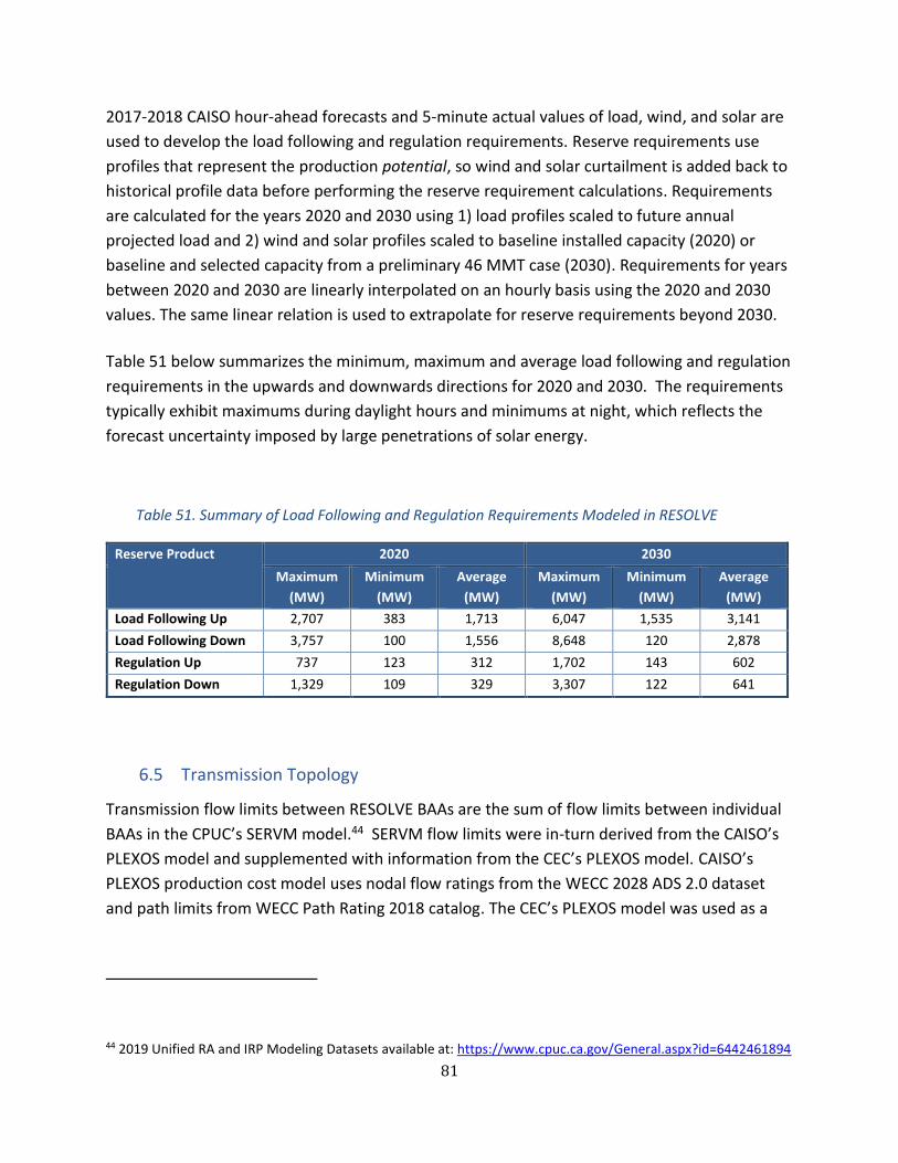
81
2017-2018 CAISO hour-ahead forecasts and 5-minute actual values of load, wind, and solar are
used to develop the load following and regulation requirements. Reserve requirements use
profiles that represent the production potential, so wind and solar curtailment is added back to
historical profile data before performing the reserve requirement calculations. Requirements
are calculated for the years 2020 and 2030 using 1) load profiles scaled to future annual
projected load and 2) wind and solar profiles scaled to baseline installed capacity (2020) or
baseline and selected capacity from a preliminary 46 MMT case (2030). Requirements for years
between 2020 and 2030 are linearly interpolated on an hourly basis using the 2020 and 2030
values. The same linear relation is used to extrapolate for reserve requirements beyond 2030.
Table 51 below summarizes the minimum, maximum and average load following and regulation
requirements in the upwards and downwards directions for 2020 and 2030. The requirements
typically exhibit maximums during daylight hours and minimums at night, which reflects the
forecast uncertainty imposed by large penetrations of solar energy.
Table 51. Summary of Load Following and Regulation Requirements Modeled in RESOLVE
Reserve Product 2020 2030
Maximum
(MW)
Minimum
(MW)
Average
(MW)
Maximum
(MW)
Minimum
(MW)
Average
(MW)
Load Following Up 2,707 383 1,713 6,047 1,535 3,141
Load Following Down 3,757 100 1,556 8,648 120 2,878
Regulation Up 737 123 312 1,702 143 602
Regulation Down 1,329 109 329 3,307 122 641
6.5 Transmission Topology
Transmission flow limits between RESOLVE BAAs are the sum of flow limits between individual
BAAs in the CPUC’s SERVM model.44 SERVM flow limits were in-turn derived from the CAISO’s
PLEXOS model and supplemented with information from the CEC’s PLEXOS model. CAISO’s
PLEXOS production cost model uses nodal flow ratings from the WECC 2028 ADS 2.0 dataset
and path limits from WECC Path Rating 2018 catalog. The CEC’s PLEXOS model was used as a
44 2019 Unified RA and IRP Modeling Datasets available at: https://www.cpuc.ca.gov/General.aspx?id=6442461894

82
supplemental data source for paths that did not have enough geographic resolution in CAISO’s
dataset.
Figure 6.2. Transmission topology used in RESOLVE (transfer limits shown in MW)
In addition to the physical underlying transmission topology, RESOLVE also includes constraints
on simultaneous net imports into, and exports out of CAISO. The net export constraint is
included to capture explicitly the uncertainty in the size of the future potential market for
California’s exports of surplus renewable power.
Table 52. Assumed CAISO net export limit (MW)
2020 2022 2026 2030
Net Export
Limit
2,000 3,000 4,000 5,000

83
Hurdle Rates
RESOLVE incorporates hurdle rates for transfers between zones; these hurdle rates are
intended to capture the transactional friction to trade energy across neighboring transmission
systems. Hurdle rates in RESOLVE are tied to the zone of export, and are derived from the
hurdle rates used in the SERVM model. SERVM hurdle rates were in-turn derived from the
CAISO’s PLEXOS model and supplemented with information from the CEC’s PLEXOS model.
RESOLVE’s NW and SW zones represent an aggregation of multiple BAAs, making it likely that
the transmission systems of multiple BAAs would be used to export energy from these regions
to CAISO. Consequently, hurdle rates to export from the NW and SW are calculated as the
average export hurdle of the constituent BAAs, plus an additional hurdle for a zone adjacent to
CAISO: APS for the SW and BPA for the NW.
Table 53. Hurdle Rates in RESOLVE ($/MWh)
Export Zone Hurdle Rate ($/MWh)
From BANC $2.42
From CAISO $10.39
From IID $3.18
From LDWP $5.59
From NW $4.91
From SW $7.35
In addition to cost-based hurdle rates, an additional cost from CARB’s cap and trade program is
added to unspecified imports into California; this cost is calculated based on the relevant year’s
carbon allowance cost and a deemed rate of 0.428 metric tons/MWh.45
Transmission Topology for Specified Imports of NW Hydro
As shown in Figure 6.3, the 2019 IRP RESOLVE model has been updated to represent specified
hydro imports from the Pacific Northwest on an hourly basis. The resource
45 Based on CARB’s rules for CARB's Mandatory Greenhouse Gas Reporting Regulation, available at:
https://ww2.arb.ca.gov/mrr-regulation

84
NW_Hydro_for_CAISO is located in a new zone called CAISO_NW_Hydro. The
CAISO_NW_Hydro zone is in between the NW and CAISO zones and does not have any load. All
unspecified imports from the NW to CAISO, and exports from CAISO to the NW, must pass
through the CAISO_NW_Hydro zone. Emissions from unspecified imports from the NW are
counted towards CAISO’s GHG limit, and incur CARB cap and trade emission permit costs using
CARB GHG intensity for unspecified imports. Transfer limits into and out of CAISO are applied to
the NW_to_CAISO transmission line between the CAISO zone and the CAISO_NW_Hydro zone.
The NW_to_CAISO line is subject to the simultaneous import and export limits between
California and the Northwest.
Figure 6.3. Transmission Topology of NW Hydro Imports in RESOLVE
6.6 Fuel Costs
Three options for fuel costs are included in RESOLVE, each of which is based on a WECC burner
tip price estimate from the CEC’s NAMGas model run posted in April 2019.46 Prices for each
RESOLVE region are aggregated from NAMGas burner tip information using the average of the
region of interest.
46 Available here: https://ww2.energy.ca.gov/assessments/ng_burner_tip.html.

85
Table 54. Fuel Cost Forecast – Low ($/MMBtu, 2016$)
Fuel Type 2020 2022 2026 2030
CA_Natural_Gas $3.64 $3.53 $3.54 $3.53
NW_Natural_Gas $3.16 $3.14 $3.16 $3.17
SW_Natural_Gas $1.90 $1.84 $1.87 $1.87
CA_Coal $2.00 $2.00 $2.00 $2.00
Coal $2.00 $2.00 $2.00 $2.00
Uranium $0.70 $0.70 $0.70 $0.70
Table 55. Fuel Cost Forecast – Mid ($/MMBtu, 2016$).
Fuel Type 2020 2022 2026 2030
CA_Natural_Gas $4.30 $4.31 $4.34 $4.36
NW_Natural_Gas $3.35 $3.36 $3.38 $3.40
SW_Natural_Gas $2.57 $2.59 $2.61 $2.64
CA_Coal $2.00 $2.00 $2.00 $2.00
Coal $2.00 $2.00 $2.00 $2.00
Uranium $0.70 $0.70 $0.70 $0.70
Table 56. Fuel Cost Forecast – High ($/MMBtu, 2016$).
Fuel Type 2020 2022 2026 2030
CA_Natural_Gas $4.92 $5.03 $5.10 $5.10
NW_Natural_Gas $3.52 $3.56 $3.58 $3.60
SW_Natural_Gas $3.15 $3.27 $3.31 $3.32
CA_Coal $2.00 $2.00 $2.00 $2.00
Coal $2.00 $2.00 $2.00 $2.00
Uranium $0.70 $0.70 $0.70 $0.70

86
The 2019-2020 IRP assumptions include three options for carbon costs. Each option is based on
revised 2019 IEPR Preliminary Nominal Carbon Price Projections.47 The carbon projections
increase 5% year-over-year in real terms. Nominal prices are converted to real $2016 for use in
RESOLVE. RESOLVE only applies these carbon prices to resources in California, as well as
unspecified imports into CAISO. 2019-2020 IRP inputs also include the option to run RESOLVE
without a carbon price via the “Zero” trajectory. The “Low” trajectory is used by default.
Table 57. Carbon Cost Forecast Options ($/tCO2, 2016$)
Fuel Type 2020 2022 2026 2030
Low $15.25 $16.84 $20.59 $25.25
Mid $17.84 $22.58 $36.26 $58.21
High $18.61 $24.55 $42.86 $74.80
Zero - - - -
47 Available at: https://efiling.energy.ca.gov/GetDocument.aspx?tn=227328&DocumentContentId=58424

87
7. Resource Adequacy Requirements
7.1 System Resource Adequacy
To ensure that the optimized generation fleet is sufficient to meet resource adequacy needs
throughout the year, RESOLVE includes a planning reserve margin constraint for the CAISO
balancing area that requires the total available generation plus available imports in each year to
meet or exceed a 15% margin above the annual 1-in-2 peak demand. The CAISO 1-in-2
managed peak demand in each year is calculated by adding or subtracting demand-side
modifiers from the baseline consumption forecast (Section 2.2). As discussed below, the
contribution of each resource to the 15% margin requirement depends on its performance
characteristics and availability to produce power during the most constrained periods of the
year.
Gas, Coal, and Nuclear Resources
The contribution of gas, coal, and nuclear generators to resource adequacy is based on CAISO’s
Net Qualifying Capacity (NQC) list. The weighted-average NQC value for each class of generator
(CCGT, CT, ST, Nuclear, etc.), expressed as a percentage of nameplate capacity, is calculated
from the NQC list for September. In RESOLVE, this percentage is multiplied by the nameplate
capacity of each class of generator to arrive at the contribution of existing and new resources
towards the planning reserve margin. For most gas, coal, and nuclear generators, these
percentages are relatively close to 100%. Note that the only coal resource in CAISO is the
Intermountain Power Plant – a dedicated import from Utah.
Table 58. Assumed Net Qualifying Capacity (NQC) for thermal generators (% of maximum capability)
Resource Class NQC (% of max)
CHP 63%
Nuclear 99%
CCGT1 94%
CCGT2 100%
Coal 98%
Peaker1 92%
Peaker2 96%
Advanced_CCGT 95%
Aero_CT 95%
Reciprocating_Engine 100%
Gas Steam (ST) 100%

88
Hydro
The NQC of existing hydroelectric resources is based on CAISO’s NQC list for September.
Demand Response
The contribution of demand response resources to the resource adequacy requirement,
including new shed DR resources selected by RESOLVE, is assumed to be equal to the 1-in-2 ex
ante peak load impact.
Renewables
Renewable resources with full capacity deliverability status (FCDS) (Section 4.2.7) are assumed
to contribute to system resource adequacy requirements. Within RESOLVE, these resources fall
into two categories: (1) firm, which includes biomass, geothermal, and small hydro; and (2)
variable resources, which includes both solar and wind resources. The treatment of each
category reflects the differences in their intermittency.
For candidate firm renewables, the contribution of each resource to resource adequacy is
assumed to be equivalent to its average annual capacity factor (i.e., a geothermal resource with
an 80% capacity factor is also assumed to have 80% net qualifying capacity). This assumption
reflects the characteristic of firm resources that they produce energy throughout the year with
a flat profile, and thereby their contribution to peak needs is not materially different from their
average levels of production throughout the year. The capacity contribution of a candidate firm
renewable resources is only counted towards the planning reserve margin constraint if
RESOLVE allocates FCDS transmission capacity to the firm resource (Section 4.2.7). The NQC of
baseline firm renewable resources is based on CAISO’s NQC list for September.
To measure the contribution of variable renewable resources to system resource adequacy
needs, RESOLVE uses the concept of “Effective Load Carrying Capability” (ELCC), defined as the
incremental load that can be met when that resource is added to a system while preserving the
same level of reliability. The contribution of wind and solar resources to resource adequacy
needs depends not only on the coincidence of the resource with peak loads, but also on the
characteristics of the other variable resources on the system. This relationship is illustrated by
the phenomenon of the declining marginal capacity value of solar resources as the “net” peak
demand shifts away from periods of peak solar production, as shown in Figure 7.1. Correctly
accounting for the capacity contribution of variable renewable resources requires a
methodology that accounts for the ELCC of the collective portfolio of intermittent resources on
the system.

89
Figure 7.1. Illustrative example of the declining marginal ELCC of solar PV with increasing penetration48
To approximate the cumulative ELCC of the CAISO’s wind and solar generators, RESOLVE
incorporates a three-dimensional ELCC surface much like the one derived for Version 6 of the
CPUC’s RPS Calculator.49 The surface expresses the total ELCC of a portfolio of wind and solar
resources as a function of the penetration of each of those two resources; each point on the
surface is the result of a single model run of E3’s Renewable Energy Capacity Planning (RECAP)
model. To incorporate the results into RESOLVE, the surface is translated into a multivariable
linear piecewise function, in which each facet of the surface is expressed as a linear function of
two variables: (1) solar penetration, and (2) wind penetration. The surface is normalized by
annual load, such that the ELCC of a portfolio of resources will adjust with increases or
decreases in load.
Each facet on the surface is a multivariate linear equation of the form fi(S,W) = aiS + biW + ci,
where fi(S,W) is the total ELCC provided by wind & solar (expressed as a percentage of 1-in-2
peak demand) and S and W represent the penetrations of solar and wind, respectively
(measured as a percentage of annual load). Because of the declining marginal ELCC of solar and
wind (and the corresponding convexity of this surface), the cumulative ELCC F(S,W) for any
penetration of wind and solar can be evaluated as the minimum of all twenty-four linear
equations: F(S,W) = min[fi(S,W)].
BTM PV is modeled as a supply-side resource within the system resource adequacy constraint,
and is therefore not represented as a demand-side modifier. Within the RESOLVE optimization,
48 For additional information see the RPSCalcWkshp_0203ResourceValuation.pptx and is located in the 02_RPS Calculator 6.0 Workshop_Feb2015 folder. Materials are available for download at: http://www.cpuc.ca.gov/WorkArea/DownloadAsset.aspx?id=9366 49Ibid

90
the capacity value of BTM PV is calculated using the ELCC value of solar as described above.
Additional adjustments are made to the planning reserve margin target to move BTM PV to the
supply side (Section 2.2.5).
Energy Storage
For energy storage, a use-limited resource, the contribution to the planning reserve margin is a
function of both the capacity and the duration of the storage device. To align with resource
adequacy accounting protocols, RESOLVE assumes a resource with four hours of duration
counts its full capacity towards the planning reserve margin, up to a capacity threshold (see the
ELCC curve below). For resources with a duration of less than four hours, the capacity
contribution is derated in proportion to the duration relative to a four-hour storage device (e.g.
a 2-hour energy storage resource receives half the capacity credit of a 4-hour resource). This
logic is applied to all baseline and candidate storage resources.
Battery storage does not provide equivalent capacity to dispatchable thermal resources at
higher battery storage penetrations because storage flattens the net peak, requiring longer
duration and/or higher stored energy volumes. Also, increasing penetrations face the
challenge of having enough energy to charge to support peak demand. Consequently, RESOLVE
includes a declining storage ELCC curve for utility-scale Li-Ion and Flow batteries that reduces
the capacity value of battery storage at higher battery storage penetrations.
Astrape consulting used the SERVM model and CPUC’s SERVM model database populated with
a preliminary RESOLVE 46 MMT portfolio to calculate the capacity contribution of storage in
2030 across a wide range of storage capacities (Figure 7.2) . The portfolio used to develop the
ELCC curve includes significant BTM and utility-scale solar capacity that can be used to charge
batteries, and may therefore overstate battery capacity value in a power system with lower
levels of solar deployment.

91
Figure 7.2. Battery Storage ELCC Curve
The marginal battery capacity value as calculated in the RESOLVE optimization, expressed as a
percentage of the battery power capacity, is equal to: Marginal ELCC [%, from Figure 7.2] *
Min(1, Duration [hours]/4 hours).
Imports
Reflecting historical levels of RA import capacity, 5 GW is used as the default assumption for
available RA import capacity (Table 59). CAISO’s contractual shares of Palo Verde, Hoover and
Intermountain Power Plant (IPP) are modeled within CAISO in RESOLVE, the capacity of these
resources (-1,937 MW in 2020) are deducted from the import capability to determine the
contribution of imports to the Planning Reserve Margin. Other options for RA import capacity
include the Maximum Import Capability into CAISO, and a “Low” option that roughly
approximates the capacity of dedicated import resources modeled in RESOLVE in 2020.
Table 59. Options for assumed import capability for resource adequacy.
RA Import Option Capacity (MW)
Maximum Import Capability (High) 11,665
Default 5,000
Low 2,000
7.2 Local Resource Adequacy Constraint
RESOLVE includes a constraint that requires that sufficient generation capacity must be
maintained or added to meet the local needs in Local Capacity Resource (LCR) areas. To

92
characterize local capacity needs, RESOLVE relies on the CAISO’s Transmission Planning Process
(TPP). The 2018-19 TPP50 does not identify any local areas as overall deficient, so RESOLVE does
not include any incremental local capacity need.
7.3 Minimum Retention of Gas-Fired Resources in Local Areas
Many dispatchable gas plants that would potentially not be economically retained by RESOLVE
are currently serving local capacity needs. While no incremental need for new capacity in local
areas is modeled in the 2019-2020 cycle, the CAISO Local Capacity Technical Study (LCT Study)51
demonstrates that electrical areas and sub-areas have limited transmission import capability.
The LCT study determines the minimum generation capacity (MW) needed to fill local needs in
case one or more transmission or generation elements is not available. CPUC Staff analysis uses
the LCT Study to determine the minimum generation capacity that comes from thermal
generation, referred to as Market Gas in the LCT Study. Market Gas values are used from the
Category C Performance Criteria by Sub-Area, meaning the situation that would result from the
loss of one element, time for adjustment, then loss of another element. The Minimum Thermal
(Market Gas) requirement is calculated as the total MW Deficiency, less the generation other
than Market Gas available in the Sub-Area. The minimum thermal requirement is allocated to
individual units using the CAISO effectiveness factors list in Attachment B of the LCT, and the
individual units are aggregated to RESOLVE generator classes. The RESOLVE optimization
enforces the minimum retention values (Table 60) for each class of generator in each year.
Table 60. Minimum gas retention
RESOLVE Resource 2030 Planned
Capacity (MW)
LCR capacity -
retained
indefinitely (MW)
Retention
decided by
RESOLVE (MW)
CAISO_CCGT1 13,333 8,412 4,921
CAISO_CCGT2 2,928 1,885 1,043
Peaker1 4,914 3,163 1,751
Peaker2 3,683 1,309 2,374
CAISO_Reciprocating_Engine 255 184 71
50 CAISO 2018-’19 Transmission Plan, Appendix D: Local Capacity Technical Analysis, available at: http://www.caiso.com/Documents/Final2019LocalCapacityTechnicalReport.pdf 51 http://www.caiso.com/informed/Pages/StakeholderProcesses/LocalCapacityRequirementsProcess.aspx

93

94
8. Greenhouse Gas Emissions and Renewables Portfolio Standard
8.1 Greenhouse Gas Constraint
RESOLVE includes optionality to enforce a greenhouse gas (GHG) constraint on CAISO
emissions. For the 2019-2020 IRP cycle, least-cost portfolios are generated in RESOLVE under
different policy assumptions about the size of the electric sector’s share, with respect to that of
other sectors, in reducing statewide GHG emissions by 2030. To set the bookends of this
analysis, staff referred to the CARB-established GHG planning target range for the electric
sector of 30–53 MMTCO2 statewide by 2030. This range is informed by the 2017 Scoping Plan
Update and further supported by CPUC’s IRP analysis in developing the 2017-2018 Reference
System Plan. As in the previous IRP cycle, the statewide emissions of the electricity sector are
be multiplied by 81%—the share of ARB’s forecasted 2030 allocation of emissions allowances to
distribution utilities within the CAISO footprint52—to yield a target for CAISO LSEs.
Table 61. Options for GHG constraints (million metric tons – CAISO footprint)
Scenario Setting 2020 2022 2026 2030
30 MMT by 2030 statewide 49.4 44.4 34.3 24.3
38 MMT by 2030 statewide 50.9 47.0 39.0 31.1
42 MMT by 2030 statewide 51.6 48.1 41.1 34.0
46 MMT by 2030 statewide 52.5 49.6 43.7 37.9
52 MMT by 2030 statewide 53.5 51.2 46,.7 42.1
Table 62. 2045 Framing Study Pathways GHG constraints (million metric tons – CAISO footprint)
Scenario Setting 2020 2022 2026 2030 2045
CEC Pathways High Electrification 50.0 45.4 36.2 26.9 10.3
CEC Pathways High Biofuels 50.4 46.1 37.4 28.8 12.3
CEC Pathways High Hydrogen 49.9 45.2 35.8 26.5 15.5
52 CARB’s allowance allocation to distribution utilities from 2021-2030 is available here: https://www.arb.ca.gov/regact/2016/capandtrade16/ attach10.xlsx

95
8.2 Greenhouse Gas Accounting
RESOLVE tracks greenhouse gas emissions attributed to entities within the CAISO footprint
using a method consistent with the California Air Resources Board’s (CARB) regulation of the
electric sector under California’s cap & trade program.
CAISO Generators
The annual emissions of generators within the CAISO is calculated in RESOLVE as part of the
dispatch simulation based on (1) the annual fuel consumed by each generator; and (2) an
assumed carbon content for the corresponding fuel.
Imports to CAISO
RESOLVE attributes emissions to generation that is imported to CAISO based on the deemed
emissions rate for unspecified imports as determined by CARB. The assumed carbon content of
imports based on this deemed rate is 0.428 metric tons per MWh53—a rate slightly higher than
the emissions rate of a combined cycle gas turbine.
Specified imports to CAISO are modeled as if the generator is located within CAISO, therefore any
emissions associated with specified imports are included with emissions associated with CAISO
generators. The majority of specified imports to CAISO are non-emitting resources, though
imports from the coal-fired Intermountain Power Plant are simulated through the mid-2020s.
Behind-the-meter CHP Emissions Accounting
CARB Scoping Plan electric sector emissions accounting includes emissions from behind-the-
meter CHP generation. BTM CHP is represented as a reduction in load in the IRP, and therefore
emissions from BTM CHP are not directly captured in RESOLVE’s generation dispatch.54 To
retain consistency with CARB’s Scoping Plan accounting conventions in the 2019-2020 IRP cycle,
emissions associated with BTM CHP generation are included under the GHG constraint, thereby
reducing the emissions budget available for supply-side resources. BTM CHP emissions are
calculated from the 2018 IEPR load forecast, totaling 5.5 MMT/yr in each year from 2020-2030.
53 Rules for CARB's Mandatory Greenhouse Gas Reporting Regulation are available here: https://ww2.arb.ca.gov/mrr-regulation 54 Due to these accounting discrepancies, in 2017 there was an estimated 4 MMT difference between RESOLVE and the Scoping Plan. Specifically, a 42 MMT target in RESOLVE was equivalent to a 46 MMT in the Scoping Plan.

96
8.3 RPS/SB100 Constraint
Senate Bill 100 (SB100) increased the state’s renewable portfolio standard to 60% by 2030 and
set a goal to supply 100% of retail electricity sales from carbon-free resources by 2045.
RPS requirement
RESOLVE includes a constraint that enforces RPS compliance in CAISO in all modeled years. This
results in the selection of a least-cost portfolio of candidate renewable resources to meet RPS
compliance, while satisfying any additional constraints. Enforcing the RPS and/or greenhouse
gas constraints (discussed in the previous section) typically result in selection of candidate
renewable resources. However, only one of these constraints will typically be binding- either
the RPS requirements will result in a lower emitting portfolio than the GHG limit, or the GHG
constraint will result in higher renewable build than the RPS requirement. Reflecting SB100,
renewables, nuclear and hydro are assumed to be RPS/SB100 eligible resources after 2030
(Figure 8.1). The retail sales compliance trajectory after 2030 is a modeling assumption and
does not reflect policy direction.
Figure 8.1. RPS/SB100 compliance
RPS Banking
As a compliance option for CAISO’s RPS requirement, RESOLVE includes the ability to retire
banked Renewable Energy Certificates (RECs) - renewable generation in excess of an LSE’s RPS
compliance requirements that can be redeemed during subsequent compliance periods. The
volume of RECs that are banked at any point in time can be material, and the timing of REC

97
redemption may significantly impact the selection of candidate resources if the RPS constraint
is driving renewable investment. For the 2019-2020 IRP cycle, RESOLVE models a specified
schedule of bank redemption (GWh in each year). This approach was used for the 2017-2018
IRP cycle. IOU’s 2018 RPS Plans are compiled to determine the starting bank in 2018. A schedule
of REC bank accrual and redemption is then calculated by comparing CAISO-wide RPS
requirements to baseline physical renewable production potential.