NBER WORKING PAPER SERIES

INPUTS IN THE PRODUCTION OF EARLY CHILDHOOD HUMAN CAPITAL:EVIDENCE FROM HEAD START

Christopher Walters

Working Paper 20639http://www.nber.org/papers/w20639

NATIONAL BUREAU OF ECONOMIC RESEARCH1050 Massachusetts Avenue

Cambridge, MA 02138October 2014

A version of this article is forthcoming at The American Economic Journal: Applied Economics. Iam grateful to Joshua Angrist, Aviva Aron-Dine, David Autor, David Card, David Chan, Hilary Hoynes,Guido Imbens, Patrick Kline, Alex Mas, Enrico Moretti, Christopher Palmer, Parag Pathak, Jesse Rothstein,Tyler Williams, two anonymous referees, and seminar participants at MIT, UC Berkeley, and the NBEREducation Program Spring meetings for useful comments and suggestions. This work was supportedby Institute for Education Sciences award number R305A120269 and a National Academy of Education/SpencerDissertation Fellowship. The views expressed herein are those of the author and do not necessarilyreflect the views of the National Bureau of Economic Research.

NBER working papers are circulated for discussion and comment purposes. They have not been peer-reviewed or been subject to the review by the NBER Board of Directors that accompanies officialNBER publications.

© 2014 by Christopher Walters. All rights reserved. Short sections of text, not to exceed two paragraphs,may be quoted without explicit permission provided that full credit, including © notice, is given tothe source.

Inputs in the Production of Early Childhood Human Capital: Evidence from Head StartChristopher WaltersNBER Working Paper No. 20639October 2014JEL No. I21,J24

ABSTRACT

Studies of small-scale "model" early-childhood programs show that high-quality preschool can havetransformative effects on human capital and economic outcomes. Evidence on the Head Start programis more mixed. Inputs and practices vary widely across Head Start centers, however, and little is knownabout variation in effectiveness within Head Start. This paper uses data from a multi-site randomizedevaluation to quantify and explain variation in effectiveness across Head Start childcare centers. Ianswer two questions: (1) How much do short-run effects vary across Head Start centers? and (2) Towhat extent do inputs, practices, and child characteristics explain this variation? To answer the firstquestion, I use a selection model with random coefficients to quantify heterogeneity in Head Starteffects, accounting for non-compliance with experimental assignments. Estimates of the model showthat the cross-center standard deviation of cognitive effects is 0.18 test score standard deviations, whichis larger than typical estimates of variation in teacher or school effectiveness. Next, I assess the roleof observed inputs, practices and child characteristics in generating this variation, focusing on inputscommonly cited as central to the success of model programs. My results show that Head Start centersoffering full-day service boost cognitive skills more than other centers, while Head Start centers offeringfrequent home visiting are especially effective at raising non-cognitive skills. Head Start is also moreeffective for children with less-educated mothers. Centers that draw more children from center-basedpreschool have smaller effects, suggesting that cross-center differences in effects may be partiallydue to differences in counterfactual preschool options. Other key inputs, including the High/Scopecurriculum, teacher education, and class size, are not associated with increased effectiveness in HeadStart. Together, observed inputs explain about one-third of the variation in Head Start effectivenessacross experimental sites.

Christopher WaltersDepartment of EconomicsUniversity of California at Berkeley530 Evans Hall #3880Berkeley, CA 94720-3880and NBERcrwalters@econ.berkeley.edu

1 Introduction

Studies of small-scale “model” early-childhood education programs show that preschool attendance can boost

outcomes in the short- and long-run. In the High/Scope Perry Preschool Project, a randomized trial that

took place in the early 1960s, 123 disadvantaged children were randomly assigned to either an intensive

preschool program or a control group without access to the program. Subsequent analyses showed that

participation in the Perry program increased average IQ at age 5 by nearly a full standard deviation, and

had lasting impacts on educational attainment, criminal behavior, drug use, employment, and earnings

(Anderson 2008; Berruta-Clement et al. 1984; Heckman et al. 2010b; Schweinhart et al. 1997, 2005).1

Heckman et al. (2010a) estimate the annual social rate of return to the Perry Project at between 7 and 10

percent. The North Carolina Abecedarian Project, another small-scale intervention, had similarly dramatic

effects (Campbell and Ramey 1994, 1995). The striking success of these programs has led some analysts to

argue that the returns to educational intervention peak early in life (Heckman 2011). These findings have

also motivated recent calls for expansion of publicly-provided preschool (Obama 2013).

In contrast, evidence on the effects of large-scale early childhood programs is more mixed. Early quasi-

experimental studies of Head Start, the largest early childhood program in the United States, showed positive

effects on cognitive skills, child mortality, and long-term outcomes (Currie and Thomas 1995; Ludwig and

Miller 2007; Garces et al. 2002; Deming 2009).2 More recently, results from the Head Start Impact Study

(HSIS), the first randomized evaluation of Head Start, showed smaller, less-persistent gains. The HSIS

experiment involved random assignment of more than 4,000 children to Head Start or a control group at

over 300 childcare centers throughout the US. The HSIS treatment group outscored the control group by

roughly 0.1 standard deviations on measures of cognitive skill during preschool, but these gains did not

persist into kindergarten (US Department of Health and Human Services 2010, 2012). Moreover, the HSIS

experiment showed little evidence of effects for a wide range of non-cognitive and health outcomes (US

Department of Health and Human Services 2010).3

Inputs and practices vary widely across Head Start centers, however, and little is known about variation

in effectiveness within Head Start. This paper uses HSIS data to quantify and explain variation in effects

across Head Start childcare centers, with an eye towards reconciling the effects of model programs and

those of Head Start. Specifically, I assess the role that inputs, practices, and child characteristics play in

generating differences in effectiveness across Head Start centers. Some centers use inputs more similar to

successful model programs than others. For example, one-third of Head Start centers use the High/Scope

curriculum, the centerpiece of the Perry Preschool experiment. Head Start centers also differ with respect

1Anderson (2008) argues that the Perry Project produced significant long-term benefits only for girls.2Other studies finding positive effects of larger-scale programs include analyses of the Chicago Child-Parent centers and

some state pre-kindergarten programs (Reynolds 1998; Gormley and Gayer 2005; Wong et al. 2008). Cascio and Schanzenbach(2013) find small effects of programs in Georgia and Oklahoma for poor children, and no effects for richer children. Fitzpatrick(2008) finds small effects for Georgia’s program, though some subgroups benefit.

3In other analyses of the HSIS data, Gelber and Isen (2013) show that Head Start participation increased parental involve-ment with children after the program ended, while Bitler et al. (2014) show larger quantile treatment effects at lower quantilesof the distribution of Peabody Picture and Vocabulary Test (PPVT) scores.

2

to teacher characteristics, class size, instructional time, frequency of home visits, and instructor experience,

all of which have been cited as central to the success of model programs (Schweinhart 2007; Chetty et al.

2011). In addition, the characteristics of Head Start applicants and the availability of alternative preschool

options vary across centers. The aim of this paper is to assess the contribution of these key inputs and

characteristics to cross-center differences in Head Start effects.

My analysis proceeds in two steps. First, to ask whether there is meaningful variation to be explained

by program characteristics, I quantify heterogeneity in causal effects across Head Start centers. This inves-

tigation is complicated by non-compliance with random assignment in the HSIS experiment. Instrumental

variables (IV) is the standard procedure for dealing with non-compliance, but IV has poor properties in

small samples, and center-specific samples in the HSIS are small (Nelson and Startz 1990). To deal with

this problem, I use a random coefficients version of the Heckman (1979) sample selection model to directly

estimate the cross-site distribution of treatment effects, circumventing the need to work with poorly-behaved

center-specific instrumental variables estimates. The random coefficients estimates reveal substantial het-

erogeneity in short-run Head Start effectiveness: the cross-center standard deviation of short-run cognitive

effects is 0.18 test score standard deviations, larger than typical estimates of variation in teacher and school

effectiveness (Deming 2013; Chetty et al. 2013a; Kane et al. 2008).

In a second step, I ask whether this variation can be explained by differences in observed program and

child characteristics. My results show that some inputs play a role: Head Start centers offering full-day

programs boost cognitive skills more than other centers, while centers offering frequent home visits are

especially effective at raising non-cognitive skills. High/Scope Head Start centers are no more effective than

other centers, however, and short-run effects are uncorrelated with teacher education, class size, and center

director experience. Short-run cognitive effects are larger for children with less educated mothers, but Head

Start effectiveness is weakly related to other measures of family background and baseline skills. To investigate

the role of alternative preschoool options, I estimate the relationship between Head Start effectiveness and

the share of children drawn from other preschools rather than home-based care. This analysis suggests that

counterfactual preschool choices play a role: cognitive gains are smaller for centers that draw more children

from center-based preschool. Together, observed inputs, practices, and child characteristics explain about

one-third of the variation in Head Start effectiveness.

An important caveat to these findings is that inputs are not randomly assigned to Head Start centers.

While the experimental variation used here eliminates selection bias in comparisons of students offered and

not offered Head Start, centers with different observed characteristics may differ systematically on unobserved

dimensions. As a result, relationships between inputs and effectiveness may not reflect causal impacts of

changing inputs in isolation. Nevertheless, these relationships are important for two reasons. First, observed

predictors of program effectiveness can help policymakers to identify high- and low-performing programs.

The ability to target high- or low-performers is useful for policies that aim to expand effective programs

or improve ineffective ones. Second, my estimates of the relationships between inputs and impacts show

3

that some key inputs used by model programs are not sufficient to create effective preschools. For example,

Schweinhart (2007) argues that the High/Scope curriculum was central to the success of the Perry Preschool

Project. I find that High/Scope is not related to program effectiveness in Head Start. This shows that the

High/Scope curriculum alone does not guarantee a successful preschool program.

In addition to the literature on preschool effects, this paper contributes to several other strands of

research. A recent series of studies relates variation in effectiveness across education programs, including

charter schools, kindergarten classrooms, and teachers, to observed program characteristics (Kane et al. 2008;

Chetty et al. 2011; Hoxby and Murarka 2009; Angrist et al. 2013; Dobbie and Fryer 2013). I apply a similar

approach to study the relationship between inputs and Head Start effects. Hotz et al. (2005), Raudenbush

et al. (2012), and Allcott (2014) analyze variation in effects across sites in multi-site randomized controlled

trials, while Chandra et al. (2013) and Syverson (2011) use empirical Bayes and random coefficients methods

to measure variation in productivity across hospitals and other firms. The analysis here includes elements

of each of these approaches.

The rest of the paper is organized as follows. The next section provides background on Head Start and

describes the HSIS data. Section 3 summarizes the average impact of Head Start on summary indices of

cognitive and non-cognitive skills. Section 4 outlines the random coefficients model used to investigate effect

heterogeneity, and reports the results of this investigation. Section 5 analyzes the link between Head Start

effectiveness and observed inputs, practices, and child characteristics. Section 6 concludes.

2 Data and Background

2.1 Head Start and the Head Start Impact Study

Head Start, the largest early-childhood program in the United States, enrolls roughly one million 3- and

4-year-old children at a cost of about $8 billion annually. The program awards grants to public, private

non-profit, and for-profit organizations that provide childcare services to children below the Federal Poverty

Line, though up to 35 percent of children attending a Head Start childcare center can be from households

between 100 and 135 percent of this income threshold. Grantees are required to match at least 20 percent of

federal Head Start funding. Head Start is based on a “whole child” model of school readiness that emphasizes

non-cognitive social and emotional development in addition to cognitive skills. The grant-based nature of

the program allows for a wide variety of childcare settings and practices, though all grantee agencies must

meet a set of program-wide performance standards (US Department of Health and Human Services 2011;

US Office of Head Start 2012).

The data used here come from the Head Start Impact Study (HSIS), a randomized evaluation of the Head

Start program. The 1998 Head Start Reauthorization Act included a congressional mandate to determine

the program’s effects. As a result, the US Department of Health and Human Services (DHHS) conducted

a nationally representative randomized controlled trial (DHHS 2010, 2012). The HSIS data includes in-

4

formation on 84 regional Head Start programs, 353 Head Start centers, and 4,442 children, each of whom

applied to a sample Head Start center in Fall 2002. Sixty percent of applicants were randomly assigned the

opportunity to attend Head Start (“treatment”), while the remaining applicants were denied this opportu-

nity (“control”). Randomization took place at the Head Start center level; the HSIS data includes weights

reflecting the probability of assignment for each child, which are used to adjust for these differences below.4

The HSIS sample includes two age groups, with 55 percent of students entering at age 3 and 45 percent

entering at age 4. Three-year-old applicants could attend Head Start for up to two years before entering

kindergarten, and three-year-olds assigned to the control group could re-apply to Head Start centers as

four-year-olds the next year. Four-year-old applicants could attend for a maximum of one year. The data

used here follow the treatment and control groups through 1st grade. DHHS (2010) provides a complete

description of the HSIS experimental design and data collection procedures. The Online Appendix details

the procedure used to construct my sample from the HSIS data.

2.2 Outcomes

The HSIS data include a large number of outcomes, collected for up to 4 years after random assignment.

I organize these outcomes into summary indices of cognitive and non-cognitive skills. Table 1 lists the

outcomes included in each group. Cognitive outcomes include scores on the Peabody Picture and Vocabu-

lary Test (PPVT) and several Woodcock Johnson III (WJIII) measures of cognitive ability. Non-cognitive

outcomes, derived from parental surveys, include measures of social skills (making friends, hitting and fight-

ing) and attention-span (concentration, restlessness). I exclude non-cognitive measures for which almost all

respondents (90% or more) gave the same answer.5

Following Kling et al. (2007) and Deming (2009), I construct indices to summarize the impact of Head

Start attendance across the outcomes listed in each column of Table 1. Specifically, I define the summary

index

Yi ≡1L

L∑`=1

(yi` − µ`σ`

), (1)

where yi` is outcome ` for student i, and µ` and σ` are the control group mean and standard deviation

of this outcome. I define outcomes so that positive signs mean better performance, and standardize them

separately by year and age cohort.

2.3 Applicant Characteristics

Head Start applicants typically come from families with low socioeconomic status. This can be seen in the

first column of Table 2, which presents mean demographic characteristics for the HSIS control group. The

4Some small centers were aggregated together to conduct the random assignment. Other centers conducted multiple roundsof random assignment with differing admission probabilities, and the HSIS weights do not account for these differences. Thediscussion in DHHS (2010) suggests that any such differences are likely to be small, however.

5The HSIS data also includes measures of non-cognitive skills reported by teachers. I do not use these measures since theyare unavailable for many children before kindergarten, and my analysis focuses on outcomes during preschool.

5

demographic variables come from a baseline survey of parents conducted in the Fall of 2002; parents of

3,577 HSIS applicants (81 percent) responded to this survey. The Head Start population is disadvantaged

on observable dimensions: roughly two-thirds of children in the sample are non-white, and about half live in

two-parent households. Thirty-nine percent of mothers in the sample did not complete high school, and 17

percent are teenagers. The average household income in the sample is $1,507 per month.6

To check experimental balance, column (2) of Table 2 shows coefficients from regressions of baseline

characteristics on assignment to Head Start, weighting by the HSIS baseline child weights to adjust for

differences in the probability of assignment across centers. The treatment/control differences in means are

statistically insignificant for all baseline variables except special needs status, and the joint p-value from a

test of the hypothesis that assignment to Head Start is unrelated to all characteristics is 0.31. This suggests

that random assignment was successful.7

The last two rows of Table 2 show the effects of assignment to Head Start on applicants’ preschool choices.

Applicants assigned to Head Start were 66 percentage points more likely to participate in the program than

applicants from the control group in the first year after random assignment. Sixteen percent of students from

the control group attended Head Start, most likely by applying to other nearby Head Start centers outside

the experimental sample. Eighteen percent of children assigned to Head Start did not participate in the

program. Together, these facts show that non-compliance with experimental assignments is an important

feature of the HSIS data, which motivates the instrumental variables approach taken below. The last row

of Table 2 shows that a Head Start offer increases the probability of attending any center-based preschool

program by 44 percentage points. This implies that two-thirds (0.442/0.663) of children induced to attend

Head Start by the experimental offer would not have attended preschool otherwise, while the remaining

one-third would have attended another preschool center if denied the opportunity to attend Head Start.

2.4 Center Characteristics

In addition to background information on applicants, the HSIS data includes detailed information on Head

Start centers and their practices. I focus on inputs and practices that have been cited as central to the

success of small-scale model programs. Schweinhart (2007) offers one view of the inputs that drove the

success of the Perry Preschool Project:

“The external validity or generalizability of the study findings extends to those programs that

are reasonably similar to the High/Scope Perry Preschool Program. A reasonably similar program

6The parent survey includes two questions about household income. One question asks for exact monthly income. Forparents who do not answer this question, a followup question asks where income falls in a set of possible categories. For parentswho answer the second question, I impute income as the midpoint of the reported range.

7Even with successful random assignment, non-random attrition has the potential to bias the experimental results. AppendixTable A1 shows attrition rates for the HSIS sample by year and outcome group, as well as treatment/control differencesconditional on the controls included in Table 4. In preschool, outcomes are observed for 82 to 84 percent of children; thefollow-up rate falls slightly in elementary school. Cognitive outcomes in preschool are observed slightly more frequently forchildren in the treatment group (3 to 5 percentage points). This modest differential attrition seems unlikely to drive the resultsreported below.

6

is a preschool education program run by teachers with bachelor’s degrees and certification in

education, each serving up to 8 children living in low-income families. The program runs 2 school

years for children who are 3 and 4 years of age with daily classes of 2.5 hours or more, uses

the High/Scope model or a similar participatory education approach, and has teachers visiting

families at least every two weeks or scheduling regular parent events.”

This account of the Perry program’s effects emphasizes six key inputs: teacher education, teacher certifi-

cation, class size, instruction time, the High/Scope curriculum, and home visiting. High/Scope is a par-

ticipatory curriculum that emphasizes childrens’ hands-on choices and experiences rather than adult-driven

instruction (Epstein 2007). Schweinhart (2007) places particular weight on the High/Scope curriculum, ar-

guing that results from the Perry Project and the followup High/Scope Preschool Curriculum Comparison

Study “[suggest] that the curriculum had a lot to do with the findings.”

No Head Start center replicates the Perry model, which used high levels of all six inputs and spent roughly

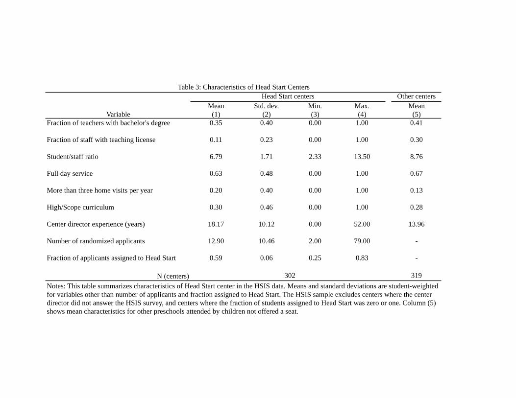
30 percent more than the average Head Start program on a per-pupil, per-year basis.8 There is substantial

variation in each of the six key Perry inputs within Head Start, however. This can be seen in Table 3,

which summarizes characteristics of centers in the HSIS sample. Thirty percent of Head Start centers use

the High/Scope curriculum. Thirty-five percent of Head Start teachers have bachelor’s degrees, and 11

percent hold teaching licenses, but the fractions with these credentials range from zero to 100 percent across

centers. The average Head Start center has 6.8 children for every staff member; the cross-center standard

deviation of class size is 1.7 children. Sixty-three percent of Head Start centers provide full-day service,

and 20 percent offer more than three home visits per year. Table 3 also reports information on years of

experience for Head Start center directors; Chetty et al. (2011) cite teacher experience as a strong predictor

of classroom effectiveness in the Tennessee STAR class size experiment. The average center director has 18

years of experience working in center-based preschools, and the standard deviation of director experience

across centers is 10 years. In Section 5, I explore whether this variation in inputs can explain differences in

effectiveness across Head Start centers.

3 Pooled Estimates

Before investigating heterogeneity in causal effects, I summarize the average impact of Head Start using

pooled equations of the form

Yi = α+ βDi +X ′iλ+ εi, (2)

where Yi is a summary index of outcomes for student i, Di is a dummy for Head Start attendance, and Xi

is a vector of the baseline controls from Table 2, included to increase precision. The attendance dummy is

8Heckman et al. (2010a) report that the Perry program cost about $17,759 per child over 2 years (2006 dollars), or $8,880per year. Per-child expenditure in Head Start was $7,600 in 2011, which is $6,800 deflated to 2006 dollars using the ConsumerPrice Index series available at http://www.bls.gov (DHHS 2011).

7

instrumented with an indicator for assignment to Head Start, Zi, with first stage equation

Di = κ+ πZi +X ′iδ + ηi. (3)

I estimate these equations by weighted two-stage least squares using the HSIS baseline child weights to

account for differences in the probability of assignment across centers. These weights multiply the inverse

probability of a child’s experimental assignment by the probability that a child’s center was sampled from the

national population (DHHS 2010). Estimates using other weighting schemes, or including center fixed effects

in equations (2) and (3), were very similar to those reported below. The coefficient β can be interpreted as a

a weighted average of center-specific local average treatment effects (LATEs), defined as effects of Head Start

attendance on students induced to attend by the experimental offer (Angrist and Imbens 1995).9 Standard

errors for these and all subsequent models allow for clustering by center of random assignment.

Estimates of equations (2) and (3) reveal that Head Start attendance boosts outcomes during preschool,

but these effects fade out quickly once children leave the program. Table 4 reports estimates of effects for

cognitive and non-cognitive skills, separately by grade and assignment cohort. Column (1) shows that in

the first year after random assignment, applicants assigned to treatment were 68 percentage points more

likely to attend Head Start than applicants in the control group. The corresponding second-stage estimates

for cognitive skills, reported in column (2), show that Head Start attendance increased cognitive skills by

0.17 standard deviations for three-year-olds and 0.09 standard deviations for four-year-olds. These estimates

are statistically significant at the 5-percent level. In contrast, estimates for non-cognitive skills, reported in

column (4), show no evidence of an effect: the point estimate for three-year-olds is positive, the estimate for

four-year-olds is negative, and neither is statistically significant.

In Spring 2004, members of the three-year-old cohort were still enrolled in Head Start. The cognitive

point estimate for this time period is comparable to the Spring 2003 estimate (0.15 standard deviations),

but is less precise (s.e. = 0.08). The decline in precision between 2003 and 2004 is driven by a decline in

compliance for the three-year-old cohort: many children in the control group re-applied to Head Start and

were admitted at age 4, reducing the first stage from 0.68 to 0.36.10 Similarly, the non-cognitive estimate

for three-year-olds in Spring 2004 is positive, but imprecise.

The remaining rows of Table 4 show that the effects of Head Start attendance dissipate once children

exit the program. The cognitive estimate for the three-year-old cohort in Spring 2005 is close to zero, and

the estimate for four-year-olds in Spring 2004 is negative and marginally significant. A positive effect of 0.1

standard deviations can be rejected at the 5-percent confidence level for the four-year-old cohort. Estimates

for both cohorts are small and statistically insignificant in later periods. Non-cognitive estimates are not

9Angrist and Imbens (1995) show that two-stage least squares estimation of a system using all center-by-treatment inter-actions as instruments produces a weighted average of center-specific LATEs, with weights proportional to the variance of thefirst stage fitted values. Estimates from this saturated model were similar to weighted least squares estimates of equations (2)and (3).

10Head Start participation in Spring 2004 is measured from the parental survey since an administrative measure of partici-pation is only available in Spring 2003. See the Online Appendix.

8

statistically distinguishable from zero in any time period for either cohort. Together, these results show little

evidence of cognitive or non-cognitive effects of Head Start after children leave preschool.

4 Variation in Head Start Effects

4.1 Variation in Instrumental Variables Estimates

I next turn to the primary contribution of this paper: Quantifying and explaining variation in short-run

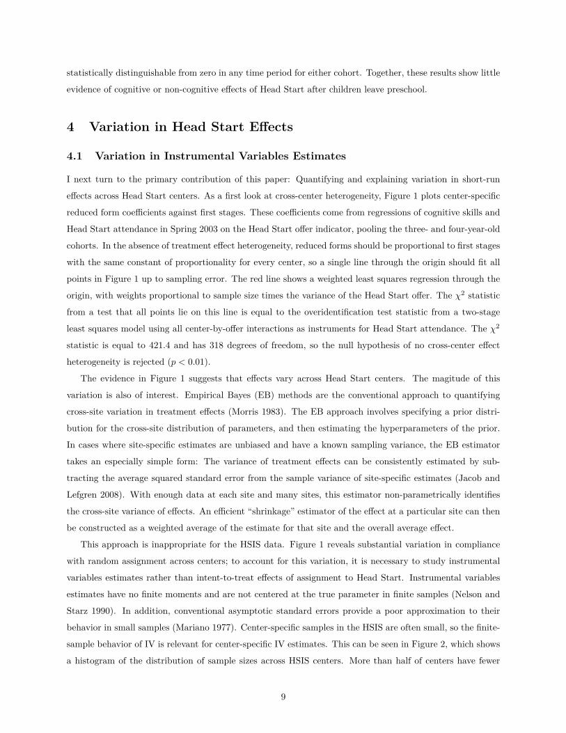
effects across Head Start centers. As a first look at cross-center heterogeneity, Figure 1 plots center-specific

reduced form coefficients against first stages. These coefficients come from regressions of cognitive skills and

Head Start attendance in Spring 2003 on the Head Start offer indicator, pooling the three- and four-year-old

cohorts. In the absence of treatment effect heterogeneity, reduced forms should be proportional to first stages

with the same constant of proportionality for every center, so a single line through the origin should fit all

points in Figure 1 up to sampling error. The red line shows a weighted least squares regression through the

origin, with weights proportional to sample size times the variance of the Head Start offer. The χ2 statistic

from a test that all points lie on this line is equal to the overidentification test statistic from a two-stage

least squares model using all center-by-offer interactions as instruments for Head Start attendance. The χ2

statistic is equal to 421.4 and has 318 degrees of freedom, so the null hypothesis of no cross-center effect

heterogeneity is rejected (p < 0.01).

The evidence in Figure 1 suggests that effects vary across Head Start centers. The magitude of this

variation is also of interest. Empirical Bayes (EB) methods are the conventional approach to quantifying

cross-site variation in treatment effects (Morris 1983). The EB approach involves specifying a prior distri-

bution for the cross-site distribution of parameters, and then estimating the hyperparameters of the prior.

In cases where site-specific estimates are unbiased and have a known sampling variance, the EB estimator

takes an especially simple form: The variance of treatment effects can be consistently estimated by sub-

tracting the average squared standard error from the sample variance of site-specific estimates (Jacob and

Lefgren 2008). With enough data at each site and many sites, this estimator non-parametrically identifies

the cross-site variance of effects. An efficient “shrinkage” estimator of the effect at a particular site can then

be constructed as a weighted average of the estimate for that site and the overall average effect.

This approach is inappropriate for the HSIS data. Figure 1 reveals substantial variation in compliance

with random assignment across centers; to account for this variation, it is necessary to study instrumental

variables estimates rather than intent-to-treat effects of assignment to Head Start. Instrumental variables

estimates have no finite moments and are not centered at the true parameter in finite samples (Nelson and

Starz 1990). In addition, conventional asymptotic standard errors provide a poor approximation to their

behavior in small samples (Mariano 1977). Center-specific samples in the HSIS are often small, so the finite-

sample behavior of IV is relevant for center-specific IV estimates. This can be seen in Figure 2, which shows

a histogram of the distribution of sample sizes across HSIS centers. More than half of centers have fewer

9

than 10 applicants, and few have more than 25.

Table 5 illustrates the poor finite-sample behavior of center-specific IV estimates for cognitive skills in

Spring 2003. The IV estimate for center j, β̂j , is the ratio of the center-specific reduced form and first

stage. The sample standard deviation of these estimates is large (1.44 test score standard deviations), and

estimates for some centers are implausible (as large as 14.8 standard deviations). The wide dispersion in

center-specific estimates is evident in Figure 3, which shows a histogram of β̂j , excluding estimates in excess

of 2 in absolute value to keep the scale reasonable.

Moreover, the asymptotic standard errors associated with these estimates yield nonsensical results. The

average standard error is 1.3 standard deviations. An estimate of the variance of βj is given by

σ̂2β = 1

J

∑j

((β̂j − β̄

)2− SE

(β̂j

)2). (4)

As a result of extremely large standard errors for some centers, this estimate is negative and large (-39.2

standard deviations), and the associated standard error shows that it is almost completely uninformative.

Since the IV asymptotic standard errors may be most inaccurate for the smallest centers, Table 5 also shows

a variance estimate that weights centers by sample size. This estimate is negative and similar in magnitude

to the unweighted estimate (-36 standard deviations); weighting improves precision, but the standard error

of the weighted variance estimate is still extremely large (35 standard deviations). These negative variance

estimates, and the associated sampling uncertainty, make it clear that the β̂j and their asymptotic standard

errors are not informative about the extent of effect heterogeneity across centers. I next describe a framework

that consistently quantifies variation in Head Start effects despite small within-center sample sizes.

4.2 Random Coefficients Framework

My approach to quantifying effect variation uses a sample selection model to describe potential outcomes

and Head Start participation conditional on Zi and center-specific parameters. I treat the parameters at

each center as draws from a prior distribution of random coefficients, and derive an integrated likelihood

function for the sample that depends only on the hyperparameters of this distribution. I then estimate the

hyperparameters by maximum likelihood. This approach circumvents the need to compute β̂j for every Head

Start center.

Let Yij(1) and Yij(0) denote potential outcomes in and out of Head Start for student i applying to Head

Start center j. Potential outcomes can be written

Yij(d) = αdj + εidj , d ∈ {0, 1}, (5)

10

where E [εidj ] = 0. The Head Start participation decision is described by

Dij = 1 {λj + πjZij > ηij} . (6)

The vector of parameters at center j is therefore

θj ≡ (α1j , α0j , λj , log πj)′ . (7)

The average effect of Head Start attendance at center j is α1j − α0j . Note that the parameter vector is

defined in terms of log πj , which guarantees that a Head Start offer weakly increases the probability of Head

Start participation for any value of θj .

I assume the following parametric structure for the within-center distribution of potential outcomes:

(εi1j , εi0j , ηij)′|Zij ∼ N (0,Σ) . (8)

Conditional on the center-specific parameters θj , assumption (8) yields a two-sided version of the Heckman

(1979) sample selection (Heckit) model. The likelihood of the observed outcomes for student i is given by

Lij(Yij , Dij |Zij ; θj) =[

Φ(σ1(λj + πjZij)− ρ1(Yij − α1j)

σ1√

1− ρ21

)1σ1φ

(Yij − α1j

σ1

)]Dij

(9)

×

[(1− Φ

(σ0(λj + πjZij)− ρ0(Yij − α0j)

σ0√

1− ρ20

))1σ0φ

(Yij − α0j

σ0

)]1−Dij

,

where σd is the standard deviation of εidj and ρd is its correlation with ηij .11

Next, I assume that the cross-center distribution of parameters follows a normal distribution:

θj |Zj ∼ N (θ0, V0) , (10)

where Zj is the vector of experimental offers for children at center j. The variance matrix V0 captures

heterogeneity in outcome distributions and experimental compliance across Head Start centers. To estimate

θ0 and V0, I integrate the site-specific parameters out of the likelihood function. The integrated likelihood

for center j is

LIj (Yj , Dj |Zj ; θ0, V0) =ˆ ∏

i

Lij (Yij , Dij |Zij ; θ)φm (θ; θ0, V0) dθ, (11)

where φm(x;µ, V ) is the multivariate normal density function. The integral in equation (11) does not have11There are two standard concerns with the Heckit model. First, without excluded instruments, the model is identified only

by functional form restrictions (Heckman 1990). This is not a problem in the present context because the Head Start offeris a strong instrument. Second, even with an excluded instrument, the functional form assumptions may be incorrect. As acheck on the plausibility of assumption (8), Appendix Table A2 compares estimates from a version of the Heckit model withno center heterogeneity to results from instrumental variables estimation. The maximum likelihood estimates of the first- andsecond-stage parameters closely match the IV estimates, suggesting that the Heckit model is not badly misspecified.

11

a closed form, so I approximate it by simulation, using 1,000 draws of θj for each Head Start center. An

empirical Bayes (EB) estimator of θ0 and V0 maximizes the sum of logarithms of simulated likelihoods

across Head Start centers.

4.3 Random Coefficients Estimates

Table 6 reports key parameter estimates from the normal random coefficients model for Spring 2003, pooling

the three- and four-year-old cohorts.12 The full set of parameter estimates is reported in Appendix Table A3.

I focus on Spring 2003 because effects for this period are largest and most precisely estimated; in addition,

the evidence in Chetty et al. (2011) suggests that immediate impacts of early-childhood programs may

predict long-run effects better than impacts in later time periods. Results for Spring 2005 are reported in

Appendix Tables A3 and A4.

The estimated parameter distributions reveal substantial heterogeneity in parameters across Head Start

centers. Consistent with the first stage estimates in Table 4, the mean compliance probability is 0.74. Com-

pliance rates vary substantially across sites: The cross-site standard deviation of the compliance probability

is 0.22. This implies that about 20 percent of centers have compliance probabilities below 0.5.

Table 6 also shows estimates of the cross-center distribution of causal effects. The estimate of the

average effect for cognitive skills is 0.11 standard deviations, while the mean non-cognitive effect is 0.02.

The cross-center standard deviation of Head Start effects, given by√V ar(α1j − α0j), is estimated to be

0.18 standard deviations for cognitive skills. This implies substantial treatment effect variation across Head

Start centers. For comparison, estimates of the standard deviations of school and teacher effectiveness are

typically around 0.1 test score standard deviations (Chetty et al. 2013a; Deming 2013; Kane et al. 2008).

My estimates therefore suggest that variation in short-run Head Start effectiveness is larger than variation

in value-added across teachers or schools. The standard deviation of effects for non-cognitive skills is smaller

(0.068 standard deviations). Figure 4 summarizes the estimated random coefficient distributions, comparing

them to histograms of center-specific first stage and IV estimates.13 The estimated parameter distributions

show much less dispersion than the distributions of center-specific estimates; nonetheless, these distributions

display substantively important heterogeneity.

The random coefficients estimates suggest that some Head Start centers have negative effects: 27 percent

of centers (Φ(−0.11/0.18)) are estimated to have cognitive effects below zero. To some extent, this is an

12Within a center, three- and four-year-old applicants sometimes faced different probabilities of assignment to Head Start.I reweight likelihood contributions to account for these differences. Specifically, the likelihood contribution of child i is Lwi

ij ,where Lij is the expression for the likelihood given in equation (11) and wi is a weight proportional to child i’s base HSISweight, normalized to sum to the total sample size.

13The first stage for center j is the difference in attendance probabilities between offered and non-offered applicants, givenby

FSj = Φ (λj + πj)− Φ (λj).

Since (λj , log πj) is assumed to be multivariate normal, the expression inside the first CDF is the sum of a normal randomvariable and a correlated log normal, which is not normally distributed. This functional form implies that the first stage isbetween 0 and 1 for all centers, a key assumption of instrumental variables models.

12

artifact of the assumed distribution for θj , which has full support on the real line. There is no reason to

expect Head Start effects to be positive for all centers or children, however. Head Start does not charge

tuition, and some parents who would otherwise spend money or time on higher-quality childcare may be

willing to forego quality in exchange for this subsidy. Cohodes and Goodman (forthcoming) find evidence of

this phenomenon in the higher education sphere: Massachusetts’ Adams Scholarship program induces some

students to substitute from expensive private institutions to less expensive public ones, reducing degree

attainment in the process.

As a check on the robustness of the random coefficient results to changes in functional form assumptions,

I estimated an alternative version of the model assuming that θj is drawn from a finite set of possible types

rather than a normal distribution. The finite-type estimates are reported in Appendix Table A5. These

estimates also suggest substantial effect heterogeneity across Head Start centers. The implied cross-center

standard deviations of effects for three- and five-type models are 0.12 and 0.22 standard deviations, roughly

similar to the normal estimate of 0.18. This result implies that the key conclusions of the random coefficients

analysis are not sensitive to the assumed functional form for the distribution of θj .

To provide further context for these estimates, I next compute the implied earnings effect of an improve-

ment in Head Start quality, using the relationships between test score effects and lifetime earnings reported

by Chetty et al. (2013b). Chetty et al. (2013b) show that a one-standard-deviation increase in teacher

value-added in a single grade translates into a 1.3 percent increase in lifetime earnings. If the mapping

between the short-run effect of Head Start on test scores and its effect on earnings is the same as this map-

ping for teachers, my results imply that a Head Start center at the 84th percentile of program quality (one

standard deviation above average) will boost lifetime earnings by 1.8 percent relative to the average Head

Start center. Assuming that children in the HSIS data will earn roughly the same amount as their parents

relative to the national median (a conservative assumption since earnings revert to the mean), and using

the same assumptions on lifetime earnings trajectories used by Chetty et al. (2013b), this translates into

an earnings effect of about $3,400 per child in 2010 dollars.14 This calculation shows that the magnitude of

cross-center variation in Head Start effectiveness is large enough to matter for later outcomes, and is also

large relative to the per-child cost of the program (roughly $7,600; DHHS 2011).

14Chetty et al. (2013b) report that the standard deviation of teacher quality is 0.13 test score standard deviations. Theyargue that a one-standard-deviation move upwards in this teacher quality distribution for one year raises students’ earningsby 1.3 percent. The implied earnings gain per standard deviation of test scores is therefore (1.3/0.13) = 10 percent. Iestimate that the standard deviation of Head Start quality is 0.18 test score standard deviations, so a one standard deviationincrease in Head Start quality boosts earnings by 0.18·10 = 1.8 percent. Chetty et al. (2013b) estimate that the meanpresent value of lifetime earnings is roughly $522,000 at age 12 in 2010 dollars, which is $434,000 discounted back to age5 at a 3-percent rate. The average HSIS family earned $18,085 per year, or 44 percent of the US median in 2002 (seehttp://www.census.gov/prod/2003pubs/p60-221.pdf). The average present discounted value of earnings at age 5 for children inthe HSIS sample can therefore be conservatively estimated as 0.44 · $434, 000 = $190,960. The earnings impact of a 1 standarddeviation increase in Head Start quality can then be approximated as $190,960·0.018= $3,437.28.

13

5 Explaining Head Start Effects

5.1 Definitions of Inputs

The estimates reported above show that some Head Start programs are substantially more effective than

others. In the remainder of the paper, I ask whether this variation in effectiveness can be explained by

observed inputs. I assess the contributions of three sets of variables: Head Start center characteristics, child

characteristics, and counterfactual preschool choices.

The analysis of center characteristics focuses on the seven variables listed in Table 3: The High/Scope

curriculum, teacher education and certification, class size, instructional time, home visting, and center

director experience. These variables are often cited as key contributors to the success of model preschool

programs (Schweinhart 2007; Chetty et al. 2011). Child characteristics include mother’s education, family

income, and baseline cognitive and non-cognitive skills. These variables seem likely to be closely linked

with human capital. The Perry Preschool Project enrolled a population of very disadvantaged children

(Schweinhart 2005). The analysis here asks whether differences in child characteristics partly explain the

difference in effectiveness between Head Start and model programs.

I also investigate the role of differences in private preschool attendance rates across centers. Children in

the HSIS sample can participate in three types of childcare: Head Start, other center-based preschool, or

home care (no preschool). As shown in Table 2, the effect of a Head Start offer on the probability of Head

Start attendance is larger than its effect on preschool attendance. This implies that some applicants would

attend other preschools in the absence of Head Start. If private preschool affects cognitive skills relative to

no preschool, differences in private preschool participation rates may drive cross-center variation in Head

Start effects even if Head Start programs are of uniform quality.

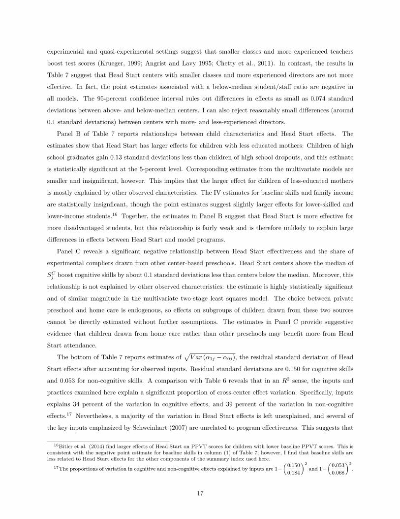
To investigate this issue, I estimate the share of students drawn into Head Start from other preschools

at center j using the regression

Cij = τCj + ρCj Zij + uCij , (12)

where Cij is an indicator for attending non-Head Start center-based preschool. The coefficient ρCj measures

the reduction in other center-based preschool attendance caused by a Head Start offer. Similarly, the share

of students drawn from no preschool is estimated using the regression

Nij = τNj + ρNj Zij + uNij , (13)

where Nij is an indicator for attending no preschool. Under the assumption that a Head Start offer does not

affect the choice of private vs. no preschool,15 the share of Head Start compliers drawn from other preschool

15This assumption can be motivated by a revealed preference argument: The availability of private preschool is unaffectedby a Head Start offer, so preferences for private vs. no preschool should not be affected by the offer. A shift between privateand no preschool in response to a Head Start offer would violate the exclusion restriction required for the offer to be a validinstrument for Head Start attendance.

14

centers is given by

SCj =(−ρCj

)(−ρNj

)+(−ρCj

) . (14)

I estimate equations (12) and (13) by weighted least squares using the HSIS child weights, setting positive

coefficients to zero to keep SCj beween zero and one. Figure 5 shows a histogram of SCj . This figure reveals

that the share of compliers who would attend other preschools in the absence of Head Start varies across

centers. At about 10 percent of centers, all compliers attend other preschools if denied the opportunity to

attend Head Start. About twenty percent of centers appear to draw children only from home care. The

remaining 70 percent draw children from a mix of private preschool and no preschool.

I investigate the relationship between inputs and Head Start effects using two approaches. First, I

estimate interacted two-stage least squares models, with second- and first-stage equations of the form

Yij = α+ P ′ijφ+ βDij +Dij · P ′ijψ +X ′ijγ + εij , (15)

Dij = κ+ P ′ijν + πZij + Zij · P ′ijτ +X ′ijδ + ηij , (16)

where Pij is a vector of child i’s characteristics and the characteristics of her center of random assignment.

The first stage equations for the interactions of Dij and Pij are analogous to equation (16). This approach

compares IV estimates for groups of centers and children with different values of Pij . Since samples at groups

of centers using different inputs are larger than samples at individual centers, this IV analysis is not subject

to the finite-sample issues discussed in Section 3. The vector ψ captures the relationship between the effect

of Head Start attendance and observed inputs. I estimate two sets of interaction models: bivariate models

that include inputs in Pij one at a time, and multivariate models that include all inputs simultaneously.

Equations (15) and (16) are estimated using binary measures of each input; for continuous variables, these

indicators equal one for centers above the sample median. An analysis using continuous measures yielded

similar but less-precise results.

Second, I extend the selection model to incorporate dependence between inputs and causal effects. The

potential outcome and selection equations are

Yij(d) = αdj + P ′ijψd + εijd, d ∈ {0, 1}, (17)

Dij = 1{λj + P ′ijν + exp

(log πj + P ′ijτ

)· Zi > ηij

}, (18)

where (εi1j , εi0j , ηij) and (α1j , α0j , λj , log πj) are assumed to be normally distributed as before. The vector

(ψ1 − ψ0) measures the relationship between inputs and Head Start effects. This approach relies in part on

parametric assumptions, so it is likely to be less robust than two-stage least squares. The advantage of the

random coefficients approach is that it generates an estimate of V0, the residual variation in center-specific

15

parameters remaining after accounting for observed inputs. It can therefore be used to measure the share of

effect heterogeneity explained by Pij .

5.2 Relationships Between Inputs and Head Start Effects

Table 7 reports the results of the analysis of inputs. Panel A shows estimates of relationships between Head

Start effectiveness and center characteristics. The estimates reveal that centers offering full-day service and

frequent home visiting are more effective. On average, cognitive effects of full-day Head Start centers are

0.14 standard deviations larger than effects of centers that do not offer this service. Corresponding estimates

for the multivariate interaction and maximum likelihood models are somewhat smaller but still statistically

significant. This implies that the relative effectiveness of full-day centers is not explained by other inputs.

Centers that offer frequent home visits per year are especially effective at raising non-cognitive skills: The

bivariate model shows that centers offering more than three home visits per year boost non-cognitive skills

by 0.11 standard deviations more than centers providing three or less visits, and this estimate is statistically

significant. The multivariate and maximum likelihood estimates show that frequent home visiting is also

associated with larger effects on cognitive skills.

The remaining estimates in Panel A of Table 7 show that other center characteristics are mostly unrelated

to Head Start effectiveness, though these estimates vary in precision. High/Scope centers do not boost scores

more than non-High/Scope centers; the interaction terms associated with High/Scope are close to zero in all

models. Moreover, this difference is precisely estimated. The hypothesis that High/Scope centers are 0.15

standard deviations more effective than other centers is rejected at the 5-percent confidence level for both

cognitive and non-cognitive skills. This result weighs against the view that the High/Scope curriculum alone

generated the success of the Perry Preschool Project.

Estimates of the relationships between Head Start effectiveness and teacher education and licensing are

statistically insignificant in most models. This result is consistent with studies of teacher value-added, which

typically find weak relationships between teacher effectiveness and credentials (Kane et al. 2008). The

estimate for teacher education is reasonably precise. In the bivariate model, the interaction coefficient on

an indicator for any staff with a bachelor’s degree is 0.026, with a standard error of 0.063. The upper

bound of the 95-percent confidence interval associated with this estimate is 0.15. The mean share with a

bachelor’s degree among centers with any bachelor’s degrees is 0.6. This implies that I can reject relatively

small differences in effects between centers that differ substantially in mean teacher education. The results

for licensing are less clear. Licensing estimates are positive in all models; the cognitive bivariate estimate is

marginally significant, and the 95-percent confidence interval in the multivariate model includes effects as

large as 0.22 standard deviations. These estimates suggest that there may be a relationship between teacher

licensing and Head Start effectiveness, but the research design used here does not have the power to detect

it.

The results for student/staff ratios and director experience are more surprising. Estimates from both

16

experimental and quasi-experimental settings suggest that smaller classes and more experienced teachers

boost test scores (Krueger, 1999; Angrist and Lavy 1995; Chetty et al., 2011). In contrast, the results in

Table 7 suggest that Head Start centers with smaller classes and more experienced directors are not more

effective. In fact, the point estimates associated with a below-median student/staff ratio are negative in

all models. The 95-percent confidence interval rules out differences in effects as small as 0.074 standard

deviations between above- and below-median centers. I can also reject reasonably small differences (around

0.1 standard deviations) between centers with more- and less-experienced directors.

Panel B of Table 7 reports relationships between child characteristics and Head Start effects. The

estimates show that Head Start has larger effects for children with less educated mothers: Children of high

school graduates gain 0.13 standard deviations less than children of high school dropouts, and this estimate

is statistically significant at the 5-percent level. Corresponding estimates from the multivariate models are

smaller and insignificant, however. This implies that the larger effect for children of less-educated mothers

is mostly explained by other observed characteristics. The IV estimates for baseline skills and family income

are statistically insignficant, though the point estimates suggest slightly larger effects for lower-skilled and

lower-income students.16 Together, the estimates in Panel B suggest that Head Start is more effective for

more disadvantaged students, but this relationship is fairly weak and is therefore unlikely to explain large

differences in effects between Head Start and model programs.

Panel C reveals a significant negative relationship between Head Start effectiveness and the share of

experimental compliers drawn from other center-based preschools. Head Start centers above the median of

SCj boost cognitive skills by about 0.1 standard deviations less than centers below the median. Moreover, this

relationship is not explained by other observed characteristics: the estimate is highly statistically significant

and of similar magnitude in the multivariate two-stage least squares model. The choice between private

preschool and home care is endogenous, so effects on subgroups of children drawn from these two sources

cannot be directly estimated without further assumptions. The estimates in Panel C provide suggestive

evidence that children drawn from home care rather than other preschools may benefit more from Head

Start attendance.

The bottom of Table 7 reports estimates of√V ar (α1j − α0j), the residual standard deviation of Head

Start effects after accounting for observed inputs. Residual standard deviations are 0.150 for cognitive skills

and 0.053 for non-cognitive skills. A comparison with Table 6 reveals that in an R2 sense, the inputs and

practices examined here explain a significant proportion of cross-center effect variation. Specifically, inputs

explains 34 percent of the variation in cognitive effects, and 39 percent of the variation in non-cognitive

effects.17 Nevertheless, a majority of the variation in Head Start effects is left unexplained, and several of

the key inputs emphasized by Schweinhart (2007) are unrelated to program effectiveness. This suggests that

16Bitler et al. (2014) find larger effects of Head Start on PPVT scores for children with lower baseline PPVT scores. This isconsistent with the negative point estimate for baseline skills in column (1) of Table 7; however, I find that baseline skills areless related to Head Start effects for the other components of the summary index used here.

17The proportions of variation in cognitive and non-cognitive effects explained by inputs are 1−(0.150

0.184

)2and 1−

(0.0530.068

)2.

17

some important drivers of successful preschool programs have yet to be identified.18

6 Conclusion

Studies of small-scale model early-childhood programs show that early intervention can boost outcomes in

the short- and long-run. Randomized evidence from the Head Start Impact Study (HSIS) suggests that

the Head Start program produces smaller short-run gains. This paper uses data from the HSIS to quantify

impact variation across Head Start centers and ask whether differences in key inputs used by model programs

can explain this variation. Estimates of a random coefficients selection model reveal substantial variation

in effectiveness across Head Start centers, particularly with respect to cognitive skills. Centers that offer

full-day service and frequent home visiting are more effective than other centers, as are centers that draw

more students from home care rather than center-based preschool. Other inputs typically cited as important

to the success of small-scale programs, including the High/Scope curriculum, teacher education, and class

size, do not predict program effectiveness in Head Start. Children of high school dropout mothers benefit

more from Head Start, but family income and baseline skills weakly predict gains. Together, observed inputs

and characteristics explain about one third of the variation in short-run cognitive effects across Head Start

centers.

It is important to emphasize that educational practices and applicant populations are not randomly

assigned to Head Start centers, so the estimates reported here may not reflect causal impacts of changing

inputs in isolation. Since Head Start centers face budget constraints, spending more on observed inputs

may require cutting spending on unobserved dimensions. As a result, my estimates may be biased towards

zero relative to the causal effects of improving inputs. Nonetheless, this analysis shows that some inputs

predict Head Start effectiveness, while others do not. The results provide no evidence that adoption of

the High/Scope curriculum or teacher education requirements would improve program effectiveness in Head

Start. This finding is relevant to recent policy changes that mandate increased education levels for Head

Start teachers (DHHS 2008). My results show that full-day service and home visiting are most predictive

of short-run Head Start effectiveness, and that efforts to target children who would not otherwise attend

preschool might boost the effects of the program. Identifying factors that explain the large residual variation

in program effectiveness is an important task for future research.

18While short-run effects are the focus of this paper, Appendix Tables A4 and A6 repeat the analysis of heterogeneity andinputs for Spring 2005. There is much less effect variation in Spring 2005 than in Spring 2003, and relationships with inputsare less precisely estimated in this period. The inputs that predict short-run gains do not seem to predict longer-run gains,which suggests that larger short-run effects are not associated with less fadeout.

18

Notes: This figure plots center-specific reduced form differences in cognitive skills in Spring 2003 against first stage differences in Head Start attendance rates. The red line comes from a weighted least squares regression through the origin, with weights proportional to NP(Z)[1 - P(Z)], where N is sample size and P(Z) is the fraction of applicants offered Head Start. The slope is 0.14 (SE = 0.03). The chi-squared statistic from a test that all points lie on the line is 421.4 (degrees of freedom = 318, p = 0.00).

Figure 1: Center-specific Reduced Forms and First Stages

-2-1

01

2R

educ

ed fo

rm

-.5 0 .5 1First stage

Figure 2: Histogram of Sample Sizes Across Head Start Centers

Notes: This figure shows the histogram of center-specific sample sizes in the HSIS experiment. The data are grouped into bins of 5 children (0 to 5, 6 to 10, etc.).

Notes: This figure plots the histogram of center-specific IV estimates for cognitive skills in Spring 2003. Estimates greater than 2 in absolute value are excluded.

Figure 3: Histogram of Center-specific IV Estimates

B. Cognitive effect C. Non-cognitive effectNotes: This figure plots maximum simulated likelihood estimates of the cross-center distributions of parameters in Spring 2003. The bars are histograms of center-specific first stage and IV estimates. The red curves are kernel density estimates produced using 200,000 draws from the distributions listed in Table A3. The densities are estimated with a triangle kernel. The bandwidth is 0.05 for panel A and 0.1 for panels B and C.

Figure 4: Estimates of Cross-center Parameter Distributions

A. First stage

01

23

4D

ensi

ty-.5 0 .5 1

First stage

0.5

11.

52

Den

sity

-2 -1 0 1 2Cognitive effect

01

23

45

Den

sity

-2 -1 0 1 2Non-cognitive effect

Figure 5: Distribution of Center-based Preschool Complier Share

Notes: This figure shows the histogram of center-specific shares of compliers attending non-Head Start center-based preschool. The data are grouped into bins of width 0.05.

0.0

5.1

.15

.2Fr

actio

n of

cen

ters

0 .2 .4 .6 .8 1Share of compliers attending center-based preschool

Cognitive skills Non-cognitive skills(1) (2)

Peabody Picture and Vocabulary Test III (PPVT) Takes care of personal thingsColor names Asks for assistance with tasks

Test de Vocabularioen Imagenes Peabody (TVIP adapted) Makes friends easilyWoodcock-Johnson III Oral Comprehension Enjoys learning

Preschool Comprehensive Test of Phonological and Print Processing (CTOPPP) Has temper tantrumsSpanish CTOPPP Cannot concentrate/pay attention for long

Woodcock-Johnson III Word Attack Is very restless/fidgets a lotMcCarthy Draw-a-design Likes to try new things

Letter naming Shows imagination in work and playWoodcock-Johnson III Letter-Word Identification Hits and fights with others

Bateria R Woodock-Munoz Identificacion de Letras y Palabras Accepts friends' ideas in playingWoodcock-Johnson III Spelling

Bateria R Woodcock-Munoz DictadoWoodcock-Johnson III Applied Problems

Woodcock-Johnson III Quantitative ConceptsCounting Bears

Bateria R Woodcock-Munoz Problemas AplicadosNotes: This table lists the cognitive and non-cognitive outcomes used in the analysis. Summary indices are averages of standardized outcomes in each category.

Table 1: Outcomes Included in Summary Indices

Control mean Offer differentialVariable (1) (2)

Male 0.490 0.011(0.023)

Black 0.259 0.009(0.011)

Hispanic 0.411 0.000(0.014)

Home language is Spanish 0.332 -0.013(0.014)

Special needs 0.112 0.020*(0.011)

Mother is married 0.478 -0.016(0.020)

Both parents live at home 0.531 -0.016(0.020)

Teen mother 0.165 -0.023(0.016)

Mother is high school dropout 0.389 -0.022(0.016)

Mother attended college 0.281 0.020(0.018)

Monthly household income 1507.124 -25.060(61.350)

Baseline cognitive skills -0.003 0.014(0.023)

Baseline non-cognitive skills 0.001 0.033(0.022)

Three-year-old cohort 0.534 -0.001(0.013)

Attended Head Start in 1st year 0.160 0.663***(0.023)

Attended any preschool in 1st year 0.460 0.442***(0.025)

Joint p-value for baseline characteristics - 0.313

N (total)N (completed survey)

Table 2: Characteristics of Head Start Applicants

4,4423,577

Notes: Column (1) shows means of baseline characteristics for Head Start applicants assigned to the control group. Column (2) shows coefficients from regressions of each characteristics on assignment to Head Start. The means and regressions are weighted using the HSIS baseline child weights. The p-value is from a test of the hypothesis that coefficients for all baseline characteristics are zero. Standard errors are clustered at the Head Start center level.***significant at 1%; **significant at 5%; *significant at 10%

Other centersMean Std. dev. Min. Max. Mean

Variable (1) (2) (3) (4) (5)Fraction of teachers with bachelor's degree 0.35 0.40 0.00 1.00 0.41

Fraction of staff with teaching license 0.11 0.23 0.00 1.00 0.30

Student/staff ratio 6.79 1.71 2.33 13.50 8.76

Full day service 0.63 0.48 0.00 1.00 0.67

More than three home visits per year 0.20 0.40 0.00 1.00 0.13

High/Scope curriculum 0.30 0.46 0.00 1.00 0.28

Center director experience (years) 18.17 10.12 0.00 52.00 13.96

Number of randomized applicants 12.90 10.46 2.00 79.00 -

Fraction of applicants assigned to Head Start 0.59 0.06 0.25 0.83 -

N (centers) 319

Table 3: Characteristics of Head Start Centers

Notes: This table summarizes characteristics of Head Start center in the HSIS data. Means and standard deviations are student-weighted for variables other than number of applicants and fraction assigned to Head Start. The HSIS sample excludes centers where the center director did not answer the HSIS survey, and centers where the fraction of students assigned to Head Start was zero or one. Column (5) shows mean characteristics for other preschools attended by children not offered a seat.

302

Head Start centers

First stage IV estimate First stage IV estimateTime period Cohort (1) (2) (3) (4)Spring 2003 3-year-olds 0.679*** 0.171*** 0.679*** 0.053

(0.031) (0.040) (0.031) (0.035)2070 2070 2062 2062

4-year-olds 0.684*** 0.088** 0.685*** -0.041(0.034) (0.037) (0.032) (0.032)1638 1638 1631 1631

Spring 2004 3-year-olds 0.362*** 0.152* 0.358*** 0.083(0.031) (0.079) (0.031) (0.071)2046 2046 2032 2032

4-year-olds 0.693*** -0.080* 0.693*** -0.035(0.033) (0.045) (0.032) (0.041)1535 1535 1555 1555

Spring 2005 3-year-olds 0.375*** -0.014 0.379*** 0.045(0.033) (0.090) (0.033) (0.088)1927 1927 1996 1996

4-year-olds 0.668*** 0.003 0.668*** -0.064(0.034) (0.062) (0.034) (0.044)1527 1527 1576 1576

Spring 2006 3-year-olds 0.367*** 0.058 0.372*** 0.030(0.032) (0.104) (0.032) (0.076)1876 1876 1957 1957

Cognitive skills Non-cognitive skillsTable 4: Effects of Head Start on Cognitive and Non-cognitive Skills by Cohort and Year

Notes: This table reports estimates of the effect of Head Start attendance on summary indices of cognitive and non-cognitive skills. Estimates come from instrumental variables models using assignment to Head Start as an instrument for Head Start attendance. All models use the HSIS baseline child weights and control for the baseline covariates listed in Table 2. Missing covariates are set to zero, and dummies for missing values are included. Standard errors are clustered at the Head Start center level.***significant at 1%; **significant at 5%; *significant at 10%

Mean Std. dev. Min. Max.(1) (2) (3) (4)

IV estimate 0.238 1.437 -4.541 14.804

IV asymptotic standard error 1.304 6.299 0.047 91.122

Unweighted:Weighted:

Implied cross-center variance of effectsNotes: This table summarizes the distribution of center-specific instrumental variables estimates for cognitive skills in Spring 2003. The estimate for each center comes from a separate IV regression of cognitive skills on Head Start attendance instrumented by Head Start assignment, pooling the 3- and 4-year-old cohorts and using the HSIS child weights.The sample excludes centers with less than 3 applicants and centers with first stages equal to exactly zero. Two other centers with small samples and first stages very close to zero are also dropped. The sample includes 286 centers. The implied cross-center variance of effects is the sample variance of the IV estimates minus the average squared standard error. The weighted variance calculation weights observations by the reciprocal of the IV standard error Standard errors of variance estimates are in parentheses.

Table 5: Finite-sample Behavior of Center-specific Instrumental Variables Estimates

-39.18 (1195.02)-35.98 (34.98)

Estimate Standard error Estimate Standard errorParameter Description (1) (2) (3) (4)

E[Φ(λj+πj) - Φ(λj)] Mean compliance probability 0.743*** 0.022 0.744*** 0.021

[Var(Φ(λj+πj) - Φ(λj))]1/2 Std. dev. of compliance probability 0.220*** 0.011 0.203*** 0.011

E[α1j] Mean treated outcome 0.105*** 0.026 0.024 0.017

E[α0j] Mean non-treated outcome -0.009 0.029 0.000 0.016

E[α1j - α0j] Mean Head Start effect 0.114*** 0.035 0.024 0.021

[Var(α1j - α0j)]1/2 Std. dev. of Head Start effects 0.184*** 0.016 0.068*** 0.007

Table 6: Random Coefficients Estimates for Spring 2003Cognitive skills Non-cognitive skills

Notes: This table lists maximum simulated likelihood estimates of parameters of the cross-center distribution of Head Start effects in Spring 2003. The sample pools the three- and four-year-old cohorts, and observations are weighted using the HSIS baseline child weights. The MSL procedure uses 1,000 simulations for each Head Start center. Standard errors are robust to misspecification and are clustered at the Head Start center level.***significant at 1%; **significant at 5%; *significant at 10%

Bivariate Multivariate Bivariate Multivariate(1) (2) (3) (4) (5) (6)

A. Center characteristicsAny staff with bachelor's degree 0.026 0.050 0.001 0.012 -0.041 -0.022

(0.063) (0.048) (0.043) (0.051) (0.050) (0.032)

Any staff have teaching license 0.127* 0.090 0.034 0.087 0.085 0.030(0.068) (0.064) (0.044) (0.052) (0.056) (0.040)

Low student/staff ratio -0.044 -0.061 -0.068 0.033 0.046 0.031(0.059) (0.050) (0.049) (0.053) (0.051) (0.032)

Full day service 0.138** 0.089* 0.083* -0.043 -0.031 -0.002(0.055) (0.047) (0.043) (0.053) (0.050) (0.031)

More than three home visits per year 0.024 0.110* 0.092* 0.112** 0.088 0.094**(0.070) (0.064) (0.055) (0.050) (0.056) (0.037)

High/Scope curriculum -0.009 0.005 -0.023 0.042 0.085 0.024(0.066) (0.054) (0.048) (0.053) (0.057) (0.035)

High center director experience 0.022 0.055 0.021 -0.011 -0.007 -0.013(0.061) (0.053) (0.044) (0.052) (0.053) (0.034)

B. Child characteristicsMother graduated high school -0.127** -0.077 -0.024 0.015 -0.010 -0.034

(0.062) (0.057) (0.042) (0.049) (0.046) (0.032)

High income -0.011 -0.003 -0.079* 0.008 0.041 0.020(0.061) (0.054) (0.044) (0.047) (0.043) (0.027)

High baseline skills -0.085 -0.004 0.019 0.023 -0.005 -0.020(0.055) (0.051) (0.035) (0.047) (0.049) (0.032)

C. Counterfactual preschool choicesHigh center-based preschool complier share -0.099* -0.117** -0.076* -0.011 -0.019 -0.004

(0.054) (0.051) (0.045) (0.047) (0.049) (0.032)

Residual std. dev. of Head Start effects - - 0.150 - - 0.053R-squared 0.337 0.393

***significant at 1%; **significant at 5%; *significant at 10%

Cognitive skills Non-cognitive skillsTable 7: Relationships Between Inputs and Head Start Effects

Notes: This table reports estimates of relationships between Head Start effects and inputs in Spring 2003. Two-stage least squares models instrument Head Start attendance and its interactions with inputs using assignment to Head Start and its interactions with inputs, with the same weighting scheme and controls as in Table 4. High (low) values of inputs are values above (below) the sample median. The bivariate models in columns (1) and (4) estimate a separate interaction model for each input, while the multivariate models in columns (2)-(3) and (5)-(6) include all interactions simultaneously. Main effects of interacting variables are included as controls. Bivariate models exclude observations with missing values for the relevant input; multivariate models exclude observations with missing values for any input. Standard errors are clustered at the Head Start center level.

Two-stage least squares Maximum likelihood

Two-stage least squares Maximum likelihood

References

1. Allcott, H. (2014). “Site Selection Bias in Program Evaluation.” Mimeo, New York University.

2. Anderson, M. (2008). “Multiple Inference and Gender Differences in the Effects of Early Intervention:A Reevaluation of the Abecedarian, Perry Preschool, and Early Training Projects.” Journal of theAmerican Statistical Association 103(484).

3. Angrist, J., and Imbens, G. (1995). “Two-stage Least Squares Estimation of Average Causal Effects inModels with Variable Treatment Intensity.” Journal of the American Statistical Association 90(430).

4. Angrist, J., and Lavy, V. (1999). “Using Maimonides’ Rule to Estimate the Effect of Class Size onScholastic Achievement.” Quarterly Journal of Economics 114(2).

5. Berruta-Clement, J., Schweinhart, L., Barnett, W., Epstein, A., and Weikart, D. (1984). ChangedLives: The Effects of the Perry Preschool Program on Youths Through Age 19. Ypsilanti, MI:High/Scope Press.

6. Bertrand, M., and Pan, J. (2013). “The Trouble with Boys: Social Influences and the Gender Gap inDisruptive Behavior.” American Economic Journal: Applied Economics 5(1).

7. Bitler, M., Domina, T., and Hoynes, H. (2014). “Experimental Evidence on Distributional Effects ofHead Start.” NBER Working Paper no. 20434.

8. Campbell, F., and Ramey, C. (1994). “Effects of Early Intervention on Intellectual and AcademicAchievement: A Follow-up Study of Children from Low-Income Families.” Child Development 65(2).

9. Campbell, F., and Ramey, C. (1995). “Cognitive and School Outcomes for High-Risk African-AmericanStudents at Middle Adolescence: Positive Effects of Early Intervention.” American Educational Re-search Journal 32(4).

10. Cascio, E., and Schanzenbach, D. (2013). “The Impacts of Expanding Access to High-Quality PreschoolEducation.” Brookings Papers on Economic Activity.

11. Chandra, A., Finkelstein, A., Sacarny, A., and Syverson, C. (2013). “Healthcare Exceptionalizm?Productivity and Allocation in the US Healthcare Sector.” NBER Working Paper no. 19200.

12. Chetty, R., Hilger, N., Saez, E., Schanzenbach, D., and Yagan, D. (2011). “How Does Your Kinder-garten Classroom Affect Your Earnings? Evidence from Project STAR.” Quarterly Journal of Eco-nomics 126(4).

13. Chetty, R., Friedman, J., and Rockoff, J. (2013a). “Measuring the Impacts of Teachers I: EvaluatingBias in Teacher Value-added Estimates.” NBER Working Paper no. 19423.

14. Chetty, R., Friedman, J., and Rockoff, J. (2013b). “Measuring the Impacts of Teachers II: TeacherValue-added and Student Outcomes in Adulthood.” NBER Working Paper no. 19424.

15. Cohodes, S., and Goodman, J. (forthcoming). “Merit Aid, College Quality, and College Completion:Massachusetts’ Adams Scholarship as an In-Kind Subsidy.” American Economic Journal: AppliedEconomics.

16. Currie, J., and Thomas, D. (1995). “Does Head Start Make a Difference?” American Economic Review85(3).

17. Deming, D. (2009). “Early Childhood Intervention and Life-Cycle Skill Development: Evidence fromHead Start.” American Economic Journal: Applied Economics 1(3).

18. Deming, D. (2013). “Using School Choice Lotteries to Test Measures of School Effectiveness.” NationalBureau of Economic Research Working Paper no. 19803.

31

19. Dobbie, W., and Fryer, R. (2011). “Are High Quality Schools Enough to Increase Achievement Amongthe Poor? Evidence from the Harlem Children’s Zone.” American Economic Journal: Applied Eco-nomics 3(3).

20. Epstein, A. (2007). Essentials of Active Learning in Preschool: Getting to Know the High/ScopeCurriculum. Ypsilanti, MI: High/Scope Press.

21. Fitzpatrick, M. (2008). “Starting School at Four: The Effect of Universal Pre-Kindergarten on Chil-dren’s Academic Achievement.” The B.E. Journal of Economic Analysis and Policy 8(1).

22. Garces, E., Thomas, D., and Currie, J. (2002). “Longer-term Effects of Head Start.” American Eco-nomic Review 92(4).

23. Gelber, A., and Isen, A. (2013). “Children’s Schooling and Parents’Behavior: Evidence from the HeadStart Impact Study.” Journal of Public Economics 101.

24. Gibbs, C., Ludwig, J., and Miller, D. (2011). “Does Head Start Do Any Lasting Good?” NationalBureau of Economic Research Working Paper no. 17452.

25. Gormley, W., and Gayer, T. (2005). “Promoting School Readiness in Oklahoma: An Evaluation ofTulsa’s Pre-K Program.” Journal of Human Resources 40.

26. Hanushek, E. (2009). “Teacher Deselection.” In: Creating a New Teaching Profession, D. Goldhaberand J. Hannaway, eds. Washington, DC: Urban Institute Press.

27. Heckman, J. (1979). “Sample Selection Bias as a Specification Error.” Econometrica 47(1).

28. Heckman, J. (1990). “Varieties of Selection Bias.” The American Economic Review 80(2).

29. Heckman, J. (2011). “The American Family in Black and White: A Post-Racial Strategy for ImprovingSkills to Promote Equality.” IZA Discussion Paper no. 5495.

30. Heckman, J., Moon, S., Pinto, R., Savelyev, P., and Yavitz, A. (2010a). “The Rate of Return to theHigh/Scope Perry Preschool Program.” Journal of Public Economics 94.

31. Heckman, J., Moon, S., Pinto, R., Savelyev, P., and Yavitz, A. (2010b). “Analyzing Social Experimentsas Implemented: A Reexamination of the Evidence from the High/Scope Perry Preschool Program.”Quantitative Economics 1(1).

32. Heckman, J., Malofeeva, L., Pinto, R., and Savelyev, P. (2013). “Understanding the MechanismsThrough Which an Influential Early Childhood Program Boosted Adult Outcomes.” American Eco-nomic Review 103(6).

33. Heckman, J., Urzua, S., and Vytlacil, E. (2006). “Understanding Instrumental Variables in Modelswith Essential Heterogeneity.” The Review of Economics and Statistics 88(3).

34. Hotz, V., Imens, G., and Mortimer, J. (2005). “Predicting the Efficacy of Future Training ProgramsUsing Past Experiences at Other Locations.” Journal of Econometrics 125(1-2).

35. Imbens, G., and Angrist, J., (1994). “Identification and Estimation of Local Average Treatment Ef-fects.” Econometrica 62(2).

36. Imbens, G., and Rubin, D. (1997). “Bayesian Inference for Causal Effects in Randomized Experimentswith Noncompliance.” Annals of Statistics 25(1).

37. Jacob, B. (2002). “Where the Boys Aren’t: Non-cognitive Skills, Returns to School and the GenderGap in Higher Education.” Economics of Education Review 21.

38. Jacob, B., and Lefgren, L. (2008). “Principals as Agents: Subjective Performance Assessment inEducation.” Journal of Labor Economics 26(1).

32

39. Kane, T., Rockoff, J., and Staiger, D. (2008). “What does Certification Tell Us About Teacher Effec-tiveness? Evidence from New York City.” Economics of Education Review 27(6).

40. Kling, J., Liebman, J., and Katz, L. (2007). “Experimental Analysis of Neighborhood Effects.” Econo-metrica 75(1).

41. Krueger, A. (1999). “Experimental Estimates of Education Production Functions.” Quarterly Journalof Economics 114(2).

42. Ludwig, J., and Miller, D. (2007). “Does Head Start Improve Children’s Life Chances? Evidence froma Regression Discontinuity Design.” Quarterly Journal of Economics 122(1).

43. Mariano, R. (1977). “Finite Sample Properties of Instrumental Variable Estimators of StructuralCoefficients.” Econometrica 45(2).

44. Morris, C. (1983). “Parametric Empirical Bayes Inference: Theory and Applications.” Journal of theAmerican Statistical Association 78(381).

45. Nelson, C., and Startz, R. (1990). “Some Further Results on the Exact Small Sample Properties ofthe Instrumental Variable Estimator.” Econometrica 58(4).

46. Obama, B. (2013). The White House, Office of the Press Secretary. Remarks by the President in stateof the union address.

47. Raudenbush, S., Reardon, S., and Nomi, T. (2012). “Statistical Analysis for Multisite Trials UsingInstrumental Variables with Random Coefficients.” Journal of Research on Educational Effectiveness5(3).

48. Reynolds, A. (1998). “Extended Early Childhood Intervention and School Achievement: Age ThirteenFindings from the Chicago Longitudinal Study.” Child Development 69(1).

49. Schweinhart, L. (2007). “How to Take the High/Scope Perry Preschool to Scale.” Paper prepared forthe National Invitational Conference of the Early Childhood Research Collaborative.

50. Schweinhart, L., Montie, J., Xiang, Z., Barnett, W., Belfield, C., and Nores, M. (2005). LifetimeEffects: The High/Scope Perry Preschool Study Through Age 40. Ypsilanti, MI: High/Scope Press.

51. Schweinhart, L., and Weikart, D. (1997). Lasting Differences: The High/Scope Preschool CurriculumComparison Study Through Age 23. Ypsilanti, MI: High/Scope Press.

52. Syverson, C. (2011). “What Determines Productivity?” Journal of Economic Literature 49(2).

53. US Department of Health and Human Services, Administration for Children and Families (2008).“Statutory Degree and Credentialing Requirements for Head Start Teaching Staff.” http://eclkc.ohs.acf.hhs.gov/hslc/standards/IMs_and_PIs_in_PDF/PDF_IMs/IM2008/ACF-IM-HS-08-12.pdf. AccessedMarch 27, 2013.

54. US Department of Health and Human Services, Administration for Children and Families (2010).“Head Start Impact Study, Final Report.” Washington, DC.

55. US Department of Health and Human Services, Administration for Children and Families (2011).“Head Start Program Facts, Fiscal Year 2011.” http://eclkc.ohs.acf.hhs.gov/hslc/mr/factsheets/docs/hs-program-fact-sheet-2011-final.pdf. Accessed March 27, 2013.

56. US Department of Health and Human Services, Administration for Children and Families (2012).“Third Grade Follow-up to the Head Start Impact Study.” Washington, DC .

57. US Office of Head Start (2012). “Head Start Services.” http://www.acf.hhs.gov/programs/ohs/about/head-start. Accessed March 27, 2013.

58. Wong, V., Cook, T., Barnett, W., and Jung, K. (2008). “An Effectiveness-based Evaluation of FiveState Pre-kindergarten Programs.” Journal of Policy Analysis and Management 27(1).

33

Online Appendix

The data for this analysis come from the Head Start Impact Study (HSIS). The HSIS data includes informa-

tion on 4,442 students. Each student applied to one of 353 Head Start centers in Fall 2002, and each center

is associated with one of 84 regional Head Start program areas. The data includes separate files with infor-

mation on test scores, answers to parental surveys, and Head Start center characteristics. This Appendix

describes the procedure used to clean each data source and construct the data set used for analysis.

Test Score Data

Test score information comes from a series of assessments conducted in Fall 2002, Spring 2003, Spring 2004,

Spring 2005 and Spring 2006. From each assessment file, I extract raw scores for the 17 tests listed in

column (1) of Table 1. These 17 tests are the main outcomes examined by DHHS (2010). The data also

include a few other tests (for example, the Leiter Sustained Attention Task), but DHHS (2010) expresses

reservations about their reliability and hence they are excluded. Not all tests were administered every year,

and there were some differences in the tests administered to Spanish-speaking and English-speaking students;

for example, the TVIP and Spanish CTOPPP were administered to Spanish speakers only. To construct

the cognitive summary index outcome, I standardize each test relative to the control group among students

who took the test separately for each cohort and assessment period. I then compute the mean of observed

standardized outcomes for each child. Finally, I append together the data sets for each assessment period,

and use a unique student identifier to reshape the data into a wide format file with one observation per

student and a separate variable for the cognitive summary index in each assessment period.

Parent Survey Data

Baseline demographics

Information on student demographics is drawn from a baseline survey of parents conducted in Fall 2002.

Eighty-one percent of households responded to this survey (3,577 of 4,442). This demographic information is

supplemented with a set of derived variables from the HSIS “Covariates and Subgroups” data file. This file

combines the baseline survey with information collected during experimental recruitment to fill in missing

values for some demographic variables. When variables are present in both files, information from the

“Covariates and Subgroups” file is used.

Non-cognitive outcomes

Indices of non-cognitive skill are constructed from the baseline parental survey and follow-up surveys

conducted in Spring 2003, Spring 2004, Spring 2005 and Spring 2006. I begin with the all social and emotional

outcomes analyzed by DHHS (2010). Each outcome is redefined so that a positive sign is favorable, and

then standardized relative to the control group separately by cohort and survey period. I also retain raw

measures of each outcome. I then append together the files for all periods. To exclude outcomes without

34

meaningful variation, I compute the mean of each raw outcome over all survey periods, and drop outcomes

where more than 90% of responses were the same. This produces the set of outcomes listed in column (2)

of Table 1. I then compute the non-cognitive summary index for each survey period as the mean of the

remaining standardized outcomes. Finally, I use the unique student identifier to reshape the data into a

wide format file with one observation per student and a separate variable for the non-cognitive summary

index in each survey period.

Measuring Head Start Assignment and Attendance

Head Start assignment comes from an administrative variable generated at the time of random assignment.

Head Start attendance in Spring 2003 is also measured administratively. To measure Head Start attendance

in later periods, I combine this administrative measure with parental survey information. Specifically, I

set Head Start attendance equal to one for Spring 2004, Spring 2005 and Spring 2006 if the Spring 2003

administrative measure is one, or if a parent indicated Head Start attendance at any time up to the relevant

time period. For time periods after Spring 2003, the Head Start attendance variable is missing for children

whose parents did not respond to the survey, because attendance cannot be accurately measured for these

students. This restriction does not affect the main results, which focus on Spring 2003.

Center Characteristics

The characteristics of Head Start centers are measured from a childcare center director survey conducted in

Spring 2003. The survey attempted to collect information from directors of all childcare centers attended by

sample children, including members of the control group who attended childcare outside of Head Start centers

in the experimental sample. The director survey data set is a student-level file, with variables capturing

responses of the center director at the center attended by each child. The seven inputs listed in Table 3 are

derived from the following questions:

• High/Scope curriculum: “If your principal curriculum has a name, what is that name?” Centers

are coded as High/Scope if the director selected High/Scope from among a list of possible answers to

this question.

• Fraction of staff with bachelors degree: “Approximately what percentage of lead and assistant

teachers in your center have a bachelors degree or higher?”

• Fraction of staff with teaching license: “Approximately what percentage of lead and assistant

teachers in your center have a teaching certificate or license?”

• Student/staff ratio: This variable is an administrative measure that divides the sum of male female

enrollment at a center by the number of staff at the center.

35

• Full-day service: “What child care options are provided at the center?” Centers are coded as full-day

if the director selected “full-day” from a list of possible responses to this question.

• More than three home visits per year: “How many home visits are required per program year?”

Directors were given a list of possible responses to this question. About 1 percent of responses were

“1 visit,” 79 percent of responses were “2-3 visits,” and 20 percent of responses were “more than three

visits.”

• Center director experience: “How many years have you worked with the following types of center-

based and child care programs?” Directors were asked to answer this question for three categories:

“Head Start,” “Non-Head Start center-based programs,” and “Non center-based child care programs.”

Director experience is measured as the sum of years spent in Head Start and non-Head Start center-

based programs.

I use these questions to derive the characteristics of each center of random assignment. To this end, I keep

observations administratively coded as both assigned to the treatment group and attending Head Start.

In some cases, codes for the center director were different for such students within a center of random

assignment. I use responses for the center director most frequently associated with treated students at a

given center of random assignment. For 7 percent of centers, there were two center director interviews

associated with an equal number of treated students. I break ties randomly to determine which responses

to use in these cases. I then keep one observation per center of random assignment. The resulting data set

has information for 89 percent (314 out of 353) of centers in the HSIS experiment.

Constructing the Analysis Data Set

The procedure described above yields 5 data files: A test score file, a baseline demographic file, a non-

cognitive outcome file, a file coding Head Start attendance after Spring 2003, and a center characteristics

file. I merge the first four of these files using a unique student identifier. I then merge the resulting file with

the center characteristics file using an identifier for center of random assignment. Finally, I merge on a sixth

file containing the HSIS baseline child weights, which yields the final data set used for analysis.

36

Follow-up rate Differential Follow-up rate DifferentialTime period Cohort (1) (2) (3) (4)Spring 2003 3-year-olds 0.842 0.027* 0.838 0.003

(0.015) (0.013)2449 2449

4-year-olds 0.814 0.047** 0.813 0.018(0.019) (0.016)1993 1993

Spring 2004 3-year-olds 0.835 0.021 0.821 0.026(0.019) (0.020)2449 2449

4-year-olds 0.770 0.009 0.780 0.015(0.022) (0.018)1993 1993

Spring 2005 3-year-olds 0.787 -0.003 0.819 0.008(0.019) (0.017)2449 2449

4-year-olds 0.766 0.010 0.781 0.026(0.025) (0.025)1993 1993

Spring 2006 3-year-olds 0.766 0.016 0.805 0.032*(0.020) (0.019)2449 2449

Notes: This table reports attrition rates for the HSIS sample. Columns (1) and (3) show fractions of children with observed outcomes by cohort and time period. Columns (2) and (4) report treatment/control differences. These differences are coefficients from regressions of a dummy for an observed outcome on treatment status, with the same controls and weighting scheme as in Table 4.***significant at 1%; **significant at 5%; *significant at 10%

Cognitive skills Non-cognitive skillsTable A1: Attrition by Cohort and Year

First stage Head Start effect First stage Head Start effectOutcome (Spring 2003) (1) (2) (3) (4)

Cognitive skills 0.681*** 0.133*** 0.719*** 0.137***(0.026) (0.030) (0.019) (0.033)

Non-cognitive skills 0.681*** 0.010 0.719*** 0.026(0.025) (0.025) (0.018) (0.021)

Table A2: Comparison of Instrumental Variables and Maximum Likelihood Estimates

***significant at 1%; **significant at 5%; *significant at 10%

Instrumental variables Maximum likelihood

Notes: This table compares parameter estimates from instrumental variables to maximum likelihood estimates of the selection model described in the text with no cross-center heterogeneity. The sample pools the three- and four-year-old cohorts. IV models use the same controls and weighting scheme as in Table 4. Standard errors are clustered at the Head Start center level.

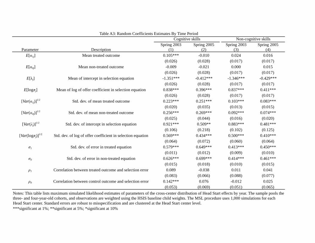
Spring 2003 Spring 2005 Spring 2003 Spring 2005Parameter Description (1) (2) (3) (4)

E[α1j] Mean treated outcome 0.105*** -0.010 0.024 0.016(0.026) (0.028) (0.017) (0.017)

E[α0j] Mean non-treated outcome -0.009 -0.021 0.000 0.015(0.026) (0.028) (0.017) (0.017)

E[λj] Mean of intercept in selection equation -1.351*** -0.412*** -1.346*** -0.429***(0.026) (0.028) (0.017) (0.017)

E[logπj] Mean of log of offer coefficient in selection equation 0.838*** 0.396*** 0.837*** 0.411***(0.026) (0.028) (0.017) (0.017)

[Var(α1j)]1/2 Std. dev. of mean treated outcome 0.223*** 0.251*** 0.103*** 0.083***(0.020) (0.035) (0.013) (0.015)

[Var(α0j)]1/2 Std. dev. of mean non-treated outcome 0.256*** 0.269*** 0.092*** 0.074***(0.025) (0.044) (0.016) (0.020)

[Var(λj)]1/2 Std. dev. of intercept in selection equation 0.921*** 0.509** 0.883*** 0.481***(0.106) (0.218) (0.102) (0.125)

[Var(logπj)]1/2 Std. dev. of log of offer coefficient in selection equation 0.569*** 0.434*** 0.500*** 0.410***(0.064) (0.072) (0.060) (0.064)

σ1 Std. dev. of error in treated equation 0.579*** 0.649*** 0.413*** 0.450***(0.011) (0.012) (0.009) (0.010)

σ0 Std. dev. of error in non-treated equation 0.626*** 0.699*** 0.414*** 0.461***(0.015) (0.018) (0.010) (0.015)

ρ1 Correlation between treated outcome and selection error 0.089 -0.038 0.011 0.041(0.083) (0.066) (0.088) (0.077)

ρ0 Correlation between control outcome and selection error 0.142*** 0.076 -0.012 0.025(0.053) (0.069) (0.051) (0.065)

Table A3: Random Coefficients Estimates By Time PeriodCognitive skills Non-cognitive skills

Notes: This table lists maximum simulated likelihood estimates of parameters of the cross-center distribution of Head Start effects by year. The sample pools the three- and four-year-old cohorts, and observations are weighted using the HSIS baseline child weights. The MSL procedure uses 1,000 simulations for each Head Start center. Standard errors are robust to misspecification and are clustered at the Head Start center level.***significant at 1%; **significant at 5%; *significant at 10%

Estimate Standard error Estimate Standard errorParameter Description (1) (2) (3) (4)

E[Φ(λj+πj) - Φ(λj)] Mean compliance probability 0.520*** 0.023 0.527*** 0.022

[Var(Φ(λj+πj) - Φ(λj))]1/2 Std. dev. of compliance probability 0.184*** 0.011 0.174*** 0.011

E[α1j] Mean treated outcome -0.014 0.029 0.019 0.018

E[α0j] Mean non-treated outcome -0.029 0.097 -0.004 0.027

E[α1j - α0j] Mean Head Start effect 0.015 0.095 0.022 0.033

[Var(α1j - α0j)]1/2 Std. dev. of Head Start effects 0.065** 0.028 0.033*** 0.007

Table A4: Random Coefficients Estimates for Spring 2005Cognitive skills Non-cognitive skills

Notes: This table lists maximum simulated likelihood estimates of parameters of the cross-center distribution of Head Start effects in Spring 2005. The sample pools the three- and four-year-old cohorts, and observations are weighted using the HSIS baseline child weights. The MSL procedure uses 1,000 simulations for each Head Start center. Standard errors are robust to misspecification and are clustered at the center level.***significant at 1%; **significant at 5%; *significant at 10%

Type 1 Type 2 Type 3 Type 1 Type 2 Type 3 Type 4 Type 5Parameter Description (1) (2) (3) (4) (5) (6) (7) (8)α1

k Mean treated outcome -0.055** 0.385*** 0.069 -0.059** 0.355*** 0.408*** 0.116 0.106(0.027) (0.033) (0.054) (0.027) (0.039) (0.095) (0.104) (0.064)

α0k Mean control outcome -0.184*** 0.249*** 0.281** -0.171*** 0.318*** -0.144 0.925*** 0.005

(0.032) (0.038) (0.133) (0.032) (0.043) (0.109) (0.192) (0.139)

α1k - α0

k Head Start effect 0.130*** 0.135*** -0.211 0.112*** 0.037 0.552*** -0.809*** 0.101(0.039) (0.046) (0.131) (0.040) (0.052) (0.137) (0.199) (0.154)

Φ(λk+πk) - Φ(λk) Compliance probability 0.760*** 0.865*** 0.214*** 0.748*** 0.842*** 0.936*** 0.552*** 0.012(0.020) (0.019) (0.079) (0.022) (0.024) (0.033) (0.103) (0.099)

Pk Type probability 0.524*** 0.344*** 0.133*** 0.518*** 0.263*** 0.097** 0.034** 0.088***(0.051) (0.045) (0.032) (0.052) (0.047) (0.039) (0.017) (0.027)

Std. dev. of Head Start effects 0.116 0.222

Three-type model Five-type modelTable A5: Maximum Likelihood Estimates of Finite-type Models

Notes: This table reports maximum likelihood estimates of finite-type models for cognitive skills in Spring 2003. Columns (1)-(3) come from a model assuming Head Start centers belong to one of three types, while columns (4)-(8) come from a model assuming centers belong to one of five types. Standard errors are robust to misspecification and are clustered at the center level.

Pk ((α1k −α0

k )− (α1 −α 0 ))2∑#$ %&1/2

Bivariate Multivariate Bivariate MultivariateVariable (1) (2) (3) (4) (5) (6)

A. Center characteristicsAny staff with bachelor's degree 0.034 0.003 0.023 0.065 0.026 -0.003

(0.077) (0.069) (0.050) (0.072) (0.069) (0.033)

Any staff have teaching license -0.012 -0.011 0.038 0.003 -0.057 -0.008(0.083) (0.084) (0.051) (0.072) (0.079) (0.036)

Low student/staff ratio -0.041 -0.044 -0.060 0.027 0.050 0.031(0.077) (0.076) (0.050) (0.071) (0.069) (0.034)

Full day service -0.035 0.000 0.043 0.014 -0.020 -0.016(0.080) (0.075) (0.049) (0.074) (0.069) (0.032)

More than three home visits per year 0.028 0.009 0.093 0.008 0.002 -0.033(0.100) (0.093) (0.061) (0.093) (0.082) (0.041)

High/Scope curriculum -0.070 -0.104 0.026 0.124* 0.123* 0.041(0.080) (0.078) (0.051) (0.069) (0.067) (0.033)

High center director experience 0.006 -0.024 0.004 0.026 0.027 0.010(0.077) (0.071) (0.050) (0.070) (0.063) (0.032)

B. Child characteristicsMother graduated high school 0.117 0.119* -0.028 -0.059 -0.108* -0.024

(0.077) (0.072) (0.054) (0.060) (0.062) (0.036)

High income -0.065 -0.105 -0.104** 0.115* 0.126** 0.016(0.080) (0.072) (0.047) (0.059) (0.058) (0.034)

High baseline skills 0.112 -0.004 -0.052 0.008 0.039 0.029(0.078) (0.066) (0.045) (0.060) (0.060) (0.036)

C. Counterfactual childcare choicesHigh center-based preschool complier share 0.059 0.080 -0.048 0.029 0.025 -0.023

(0.074) (0.078) (0.052) (0.061) (0.063) (0.031)

Residual std. dev. of Head Start effects - - 0.062 - - 0.027R-squared 0.099 0.345

Notes: This table reports estimates of relationships between Head Start effects and inputs in Spring 2005. Two-stage least squares models instrument Head Start attendance and its interactions with inputs using assignment to Head Start and its interactions with inputs, with the same weighting scheme and controls as in Table 4. Columns (1) and (4) estimate a separate interaction model for each input, while columns (2)-(3) and (5)-(6) include all interactions simultaneously. Main effects of interacting variables are included as controls. Standard errors are clustered at the Head Start center level.***significant at 1%; **significant at 5%; *significant at 10%

Table A6: Relationships Between Inputs and Head Start Effects in Spring 2005Cognitive skills Non-cognitive skills

Two-stage least squares Maximum likelihood

Two-stage least squares Maximum likelihood