Inspecting the Mechanism:

Leverage and the Great Recession in the Eurozone∗

Philippe Martin†and Thomas Philippon‡

May 2015

Abstract

We provide a comprehensive account of the dynamics of eurozone countries from 2000 to 2012.

We analyze private leverage, fiscal policy, labor costs and interest rates and we propose a strategy

to separate the impact of credit cycles, excessive government spending, and sudden stops. We

then ask how eurozone countries would have fared with different policies. We find that most

countries could have stabilized their employment if they had followed more conservative fiscal

policies during the boom. Macro-prudential policies and an early intervention by the central

bank to prevent market segmentation would also have significantly reduced the recession.

JEL Codes: E00, E62, F41, F44, F45, G01

∗We thank Pierre Olivier Gourinchas, Nobu Kiyotaki, Fiorella De Fiore, Emi Nakamura, Vania Stavrakeva, IvanWerning and Philip Lane for their discussions, as well as Mark Aguiar, Olivier Blanchard, Ariel Burstein, GiovanniDell’Arricia, Gita Gopinath, Gianluca Violante, Caterina Mendicino, Mark Gertler, Virgiliu Midrigan and seminarparticipants at AEA, NY Fed, NYU, Harvard, Berkeley, Oxford, IMF, Warwick, Maryland, TSE, PSE, Banquede France, CREI, ECB, Warwick, ESSIM-CEPR, the NBER IF and the NBER EFG for their comments. JosebaMartinez provided outstanding research assistance. We thank the Fondation Banque de France for financial support.Philippe Martin is also grateful to the Banque de France Sciences Po partnership for its financial support.

†Sciences Po and CEPR‡New York University, CEPR and NBER

1

1 Introduction

The lesson to be learned from the crisis is that a currency union needs ironclad budget

discipline to avert a boom-and-bust cycle in the first place. Hans Werner Sinn (2010)

On the eve of the crisis (Spain) had low debt and a budget surplus. Unfortunately, it

also had an enormous housing bubble, a bubble made possible in large part by huge loans

from German banks to their Spanish counterparts. Paul Krugman (2012)

The situation of Spain is reminiscent of the situation of emerging economies that have

to borrow in a foreign currency...they can suddenly be confronted with a “sudden stop”

when capital inflows suddenly stop leading to a liquidity crisis. Paul de Grauwe (2012)

Countries which lost competitiveness prior to the crisis experienced the lowest growth

after the crisis. Lorenzo Bini Smaghi (2013)

These quotes illustrate a persistent disagreement about the best way to interpret the eurozone crisis.

Some argue that the crisis stems from a lack of fiscal discipline, some emphasize excessive private

leverage, while others focus on sudden stops or competitiveness divergence due to fixed exchange

rates. Most observers understand that all these factors have played a role, but do not offer a way

to quantify their respective importance. In this context it is difficult to frame policy prescriptions

on macroeconomic policies and on reforms of the eurozone. Moreover, given the scale of the crisis,

understanding the dynamics of the eurozone is one of the major challenge for macroeconomics today.

In this context, we propose a quantitative model to understand the dynamics of countries within

the eurozone.

The ultimate goal of this paper is to perform counterfactual experiments. For instance, we want

to understand what would have happened to a particular country if it had run a different fiscal policy

during the boom years, or if the eurozone had been able to prevent sudden stops. Our contribution

is to propose a model and an identification strategy to answer these questions. Needless to say, this

is a difficult task that requires several steps: (i) specify a model and collect the data; (ii) find an

identification strategy; (iii) run counterfactual experiments.

We analyze the dynamics of private debt, fiscal policy, and funding costs in a collection of small

open economies within a monetary union. Each economy has an independent fiscal authority and

is populated by patient and impatient agents. Impatient agents borrow from patient agents at

home and abroad, and are subject to time-varying borrowing limits. Governments borrow, tax, and

spend. Funding costs are linked to private and public debt sustainability. Nominal wages adjust

slowly and changes in nominal expenditures affect employment.

Business Cycle Accounting in the Eurozone Our first contribution is to perform a business

cycle accounting exercise for the eurozone. We show that the parsimonious model outlined above

does a fairly good job at replicating the dynamics of each country from 2000 to 2012. It is important

to emphasize that we focus on the dynamics of each country relative to the eurozone average. This

2

approach helps us identify the model by netting out some aspects of monetary policy and exchange

rate fluctuations. For instance, we seek to explain relative employment and inflation in Spain, but

not aggregate employment and inflation in the eurozone. We show that, given the relative paths of

private debt, government spending and interest rates from 2000 to 2012, the model predicts fairly

well the relative paths for GDP, employment, inflation, net exports, etc. All the driving variables

are directly observable and the model has very few degrees of freedom.

It is clear, however, that this exercise cannot tell us what caused the recessions in different

countries. Private debt, fiscal policy and funding costs are endogenous equilibrium objects, and we

want instead to identify “sudden stop” shocks, “private lending” shocks, and “discretionary” fiscal

choices. All these shocks affect interest rates, debt dynamics, and via general equilibrium effects

and policy responses, output and employment. We therefore need an identification strategy.

Identification Strategy The strategy we propose is based on a combination of functional re-

strictions, instrumental variable regressions, and the use of a control group.

We first specify the decision rule that pins down government spending as a function of the state

of the economy. We assume that the government seeks to stabilize employment near its natural

rate, cuts spending in response to an increase in borrowing costs, and is subject to a country-specific

spending bias. The first two components of the decision rule are the same in all countries. The

third component contains one parameter per country, which is the bias needed to reconcile actual

and predicted average spending during the boom. We estimate a small (essentially zero) “political

economy” bias in several countries, such as Germany and Portugal, and a large one in some other

countries, such as Greece for instance.

We then model sudden stops as a common risk factor that increases after 2008, and we show that

it materializes in countries with high public and private debts, including implicit liabilities linked

to bank recapitalization costs. We use instrumental variables to estimate the impact of public and

private debts on the economy’s cost of funds, assuming that governments did not anticipate that a

crisis would come at the end of the boom.

The last identification issue is the most difficult. We need to ascertain how the sudden stop

affects the dynamics of private debt. This is complicated because private deleveraging can happen

even without sudden stop and because we are not willing to impose the same restrictions regarding

functional forms and anticipations on private agents as we impose on governments. Our key idea

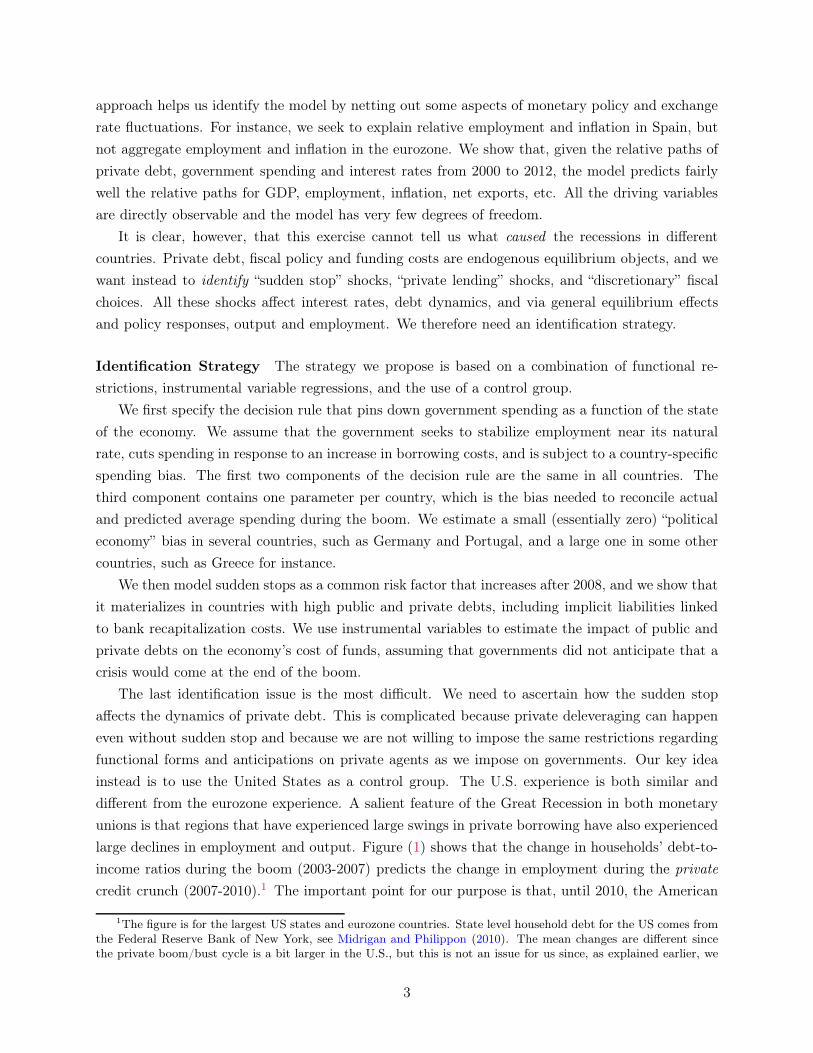
instead is to use the United States as a control group. The U.S. experience is both similar and

different from the eurozone experience. A salient feature of the Great Recession in both monetary

unions is that regions that have experienced large swings in private borrowing have also experienced

large declines in employment and output. Figure (1) shows that the change in households’ debt-to-

income ratios during the boom (2003-2007) predicts the change in employment during the private

credit crunch (2007-2010).1 The important point for our purpose is that, until 2010, the American

1The figure is for the largest US states and eurozone countries. State level household debt for the US comes fromthe Federal Reserve Bank of New York, see Midrigan and Philippon (2010). The mean changes are different sincethe private boom/bust cycle is a bit larger in the U.S., but this is not an issue for us since, as explained earlier, we

3

and European experiences look strikingly similar. In both cases, there is a significant dispersion

of leverage and employment, a very good fit, and (almost) the same slopes. This suggests similar

structural parameters governing the endogenous propagation mechanism.

Figure 1: First Stage of the Great Recession: Household Borrowing predicts Employment Bust inthe US and the EZ

AZ

CA

FL

IL

MI

NJ

NV

NY

OH

PATX

USA

AUT

BEL

DEU

ESP

FIN

FRA GRE

IRL

ITA

NLD

PRT

−.06

−.04

−.02

0.0

2Ch

ange

Em

p/Po

p 20

07−2

009

−.1 .1 .3 .5Change Household Debt/GDP 2003−2007

A significant difference between the two regions appears only after 2010 when the eurozone

experiences sudden stops, financial fragmentation, and sovereign debt crises coupled with the risk

of a breakup of the currency union.2 States within the U.S. do not experience sudden stops, but

they reduce their private leverage nonetheless. Our identification strategy is then to use actual

private debt dynamics across the U.S. to construct predicted debt series across eurozone countries.

We argue that these are the private debt dynamics that would prevail in the eurozone without

financial fragmentation. Importantly, these predicted debt series are far from constant and failure

to recognize this fact would lead to severe biases in the estimations of the true causes of the eurozone

crisis.

Structural Model and Counter-Factual Experiments Our structural model therefore fea-

tures endogenous private debt, fiscal policy and cost of funds. The exogenous driving forces are a

time varying risk of sudden stop (one time series), country specific political economy biases (one

number per country), and the predicted private debt series (one time series per country). We show

that this structural model fits the data well. Given the exogenous driving forces, the model predicts

fairly well the relative paths of GDP, employment, inflation, net exports, public debt and private

focus on dynamics relative to the average.2Sudden stops were frequent in the 19th and 20th centuries but we do not know of any other historical example

of a sudden stop inside a monetary union. See Accominotti and Eichengreen (2013).

4

debt from 2000 to 2012. This is a demanding exercise since we ask the model to predict the booms,

the turning points and the busts for all the series and all the countries.

The critical advantage of the structural model – compared to the model that takes as given the

paths of private debt, government spending and spreads, as explained above – is that we can use

the structural model to perform counterfactual experiments. We perform four such experiments.

We first ask how countries would have fared if they had followed more conservative fiscal policies

during the boom. To do so, we shut down the “political economy spending bias” of the structural

model. We find that such policies lead to lower spreads and less need for fiscal austerity during the

bust. Periphery countries partially stabilize their employment. This is especially true for Greece,

and to a lesser extent for Ireland and Spain. For Ireland, however, this more conservative policy

requires buying back the entire stock of public debt, which suggests that fiscal policy is unlikely to

be enough as a stabilization tool against a large credit boom.

We then ask how these countries would have fared if they had conducted macro-prudential

policies to limit the increase in private debt. This policy stabilizes private demand and therefore

employment, and it reduces the need for bank recapitalization, leading to lower spreads and more

room for countercyclical fiscal policy, especially in Ireland. Our experiment also uncovers a new

interaction between macro-prudential and fiscal policies. A biased government substitutes public

debt for private debt in response to restrictive macro-prudential policy, thereby undoing some of

the macro-prudential benefits. This suggests a complementarity between fiscal rules and macro-

prudential rules.

In a third counterfactual experiment, we assume that the European Central Bank’s OMT pro-

gram (and Mario Draghi’s “Whatever it takes” speech) is announced in 2008 rather than in 2012.

This reduces the risk of a breakup of the eurozone, prevents the increase in spreads, and allows

the four periphery countries to stabilize employment after 2010. Interestingly, the counter-factual

employment dynamics across the eurozone then look similar to the observed dynamics across the

United States.

In our last counterfactual, we let countries engineer a 10% fiscal devaluation in 2009. This

generates a boom in exports, a shorter and milder recession, and a successful fiscal adjustment with

a lower public debt in 2012. Overall, our results are consistent with many policy makers’ beliefs

about the crisis, but we are the first to formalize and quantify them.

Literature review Our paper is most directly related to three lines of research: macro-economic

models with credit frictions, in particular that of Eggertsson and Krugman (2012); open-economy

models with interest rates shocks, as in Neumeyer and Perri (2005); and analyses of the eurozone

crisis such as Lane (2012) for instance.

Kiyotaki and Moore (1997), Bernanke et al. (1999) and Gertler and Kiyotaki (2010) consider

credit constraints that limit corporate investment, while we put more emphasis on household credit,

as Mian and Sufi (2012), Midrigan and Philippon (2010) and Eggertsson and Krugman (2012). This

difference matters mostly when we fit the model with cross-sectional data. A striking feature of

5

the data is the strong correlation between household leverage and employment at the micro-level.

Mian and Sufi (2012) show that differences in household debt overhang explains why unemployment

is higher in some counties than in others. These facts are not easily explained by a “local lending

channel” or by credit constraints that operate only at the firm level, presumably because business

lending is not very localized in the U.S.3

The literature on sudden stops in emerging markets focuses on the rapid imposition of an

external credit constraint, and usually emphasizes Fisherian amplification when debts and in-

comes are denominated in different currencies (see Christiano and Roldos 2004; Chari et al. 2005;

Mendoza and Smith 2006; Mendoza, 2010; Korinek and Mendoza 2013). The sudden stops them-

selves can be explained by multiple equilibria in international financial markets with transaction

costs, as in Martin and Rey (2006). By contrast, we focus on countries that belong to a monetary

union and our model integrates, for the first time to our knowledge, both domestic and external

debt dynamics. This is critical for understanding the eurozone crisis since, as we have explained,

private deleveraging would have created a recession even without an external credit constraint.

In Neumeyer and Perri (2005) interest rates shocks, either exogenous or induced by productivity

shocks, generate sudden stops and current account reversals because they induce a working capital

shortage. In our model, the increase in interest rates generates a demand shock through a fall in

private and public expenditures.

Our business cycle accounting exercise is similar in spirit to the work of Chari et al. (2007) but

we emphasize different shocks. While most of the sudden stop literature has emphasized credit

constraints, Gopinath (2004) and Aguiar and Gopinath (2007) have focused on TFP shocks. In

Aguiar and Gopinath (2007) a negative shock to trend growth leads to a fall in consumption and an

increase in the trade balance.4 TFP shocks are certainly important in emerging markets, but they do

not seem to explain the dynamics of euro area countries during the great recession. Countries hit by

sudden stops (Greece, Ireland, Italy, Spain, Portugal) do not experience the largest reversals in trend

TFP growth, and there is no correlation between changes in TFP growth and employment losses

during the recession (see figure (21) in Appendix B.1). In fact, the only country that shows signs of

TFP growth during the boom years is Greece, but the reliability of these numbers is questionable.

Our paper is related to the literature on sovereign credit risk (see Eaton and Gersovitz 1982;

Arellano 2008; Mendoza and Yue 2012) but we do not actually model strategic default decisions.

We focus instead on how sovereign default risk affects the real economy. Corsetti et al. (2013) model

3Mian and Sufi (2010) find that the predictive power of household borrowing remains the same in counties dom-inated by national banks. It is also well known that businesses entered the recession with historically strong balancesheets and were able to draw on existing credit lines, as shown by Ivashina and Scharfstein (2008). On the other hand,our model is perfectly consistent with firm level credit constraints in addition to household level credit constraints, asdiscussed recently by Giroud and Mueller (2015). Our approach is also consistent with the lending constraints viewof Justiniano et al. (2014).

4Gopinath (2004) proposes a model with a search friction to generate asymmetric responses to symmetric shocks.A search friction in foreign investors’ entry decision into emerging markets creates an asymmetry in the adjustmentprocess of the economy: An increase in traded sector productivity raises GDP on impact, and it continues to growto a higher long-run level. On the other hand, a decline in traded sector productivity causes GDP to contract in theshort run by more than it does in the long-run. Aguiar and Gopinath (2007) do not study the response of the labormarket but it is well known that income effects tend move consumption and hours in opposite directions.

6

such a “sovereign risk channel” through which sovereign default risk raises the private sector cost of

funds. A high cost of funds forces the government to cut spending and our model is qualitatively

and quantitatively consistent with the recent research on fiscal multipliers at the regional level (see

Nakamura and Steinsson, 2014; Farhi and Werning 2013).

The papers by Lane (2012) and Shambaugh (2012) provide a thorough description of the

four dimensions of the eurozone crisis: public debt, private debt, sudden stop and competitive-

ness. The specific role of the boom/bust cycle in capital flows is analyzed by Lane (2013) while

Gourinchas and Obstfeld (2012) show that domestic credit expansion is the most robust predictor of

financial crises. Battistini et al. (2014) argue that the perceived risk of a eurozone breakup is a key

driver of financial fragmentation during the crisis. Schmitt-Grohe and Uribe (2012) emphasize the

role of downward wage rigidity. Some papers also compare and describe the specific circumstances

of individual countries. Fernández Villaverde et al. (2013) argue that loose financing conditions and

capital inflows following the creation of the euro relaxed the pressure for reforms in the four periph-

ery countries. Reis (2013) argues that capital misallocation explains the low growth of Portugal

between 2000 and 2007. Whelan (2014) stresses the role of cheap credit and lax banking regulation

in Ireland, and Cunat and Guadalupe (2009) analyzes the lending behavior of the Spanish Cajas in

the run up to the crisis. While our model cannot do justice to the specificities of every single coun-

try, it nonetheless gives an interpretation of the crisis that is consistent with the views expressed in

these various papers.

The remaining of the paper is organized as follows. In Section 2 we present the model and in

section 3 we analyze its dynamic properties. Section 4 compares the predictions of the reduced form

model to the data. In Section 5 we estimate the structural relations between private leverage, fiscal

policy and sudden stops. The structural model is used to conduct our counterfactual experiments

in section 6. Section 7 concludes. There are also several Appendices presenting the data sources,

the various adjustments that need to be made to the raw data, the details of the model, and the

simulations.

2 Model

We model a currency union with several regions. We follow Gali and Monacelli (2008) and study

a small open economy that trades with other regions. Each region j produces a tradable domestic

good and is populated by households who consume the domestic good and a basket of foreign

goods. Following Mankiw (2000) and more recently Eggertsson and Krugman (2012), we assume

that households are heterogenous in their degree of time preference. More precisely, in region j,

there is a fraction χj of impatient households, and 1 − χj of patient ones. Patient households

(indexed by i = s for savers) have a higher discount factor than borrowers (indexed by i = b for

borrowers): β ≡ βs > βb. Saving and borrowing are measured in units of the common currency

(euros).

7

2.1 Within period trade and production.

Consider household i in region j at time t. Within period, all households have the same log

preferences over the consumption of home goods (h), foreign goods (f), and labor supply:

ui,j,t = αj log

!

Chi,j,t

αj

"

+ (1− αj) log

!

Cfi,j,t

1− αj

"

− ν (Ni,j,t)

With these preferences, households of region j spend a fraction αj of their income on home goods,

and 1 − αj on foreign goods. The parameter αj measures how closed the economy is, because of

home bias in preferences or trade costs. The demand functions are then:

P hj,tC

hi,j,t = αjXi,j,t,

P ft C

fi,j,t = (1− αj)Xi,j,t.

where

Xi,j,t ≡ P hj,tC

hi,j,t + P f

t Cfi,j,t

measures total spending by household i in region j in period t, P hj,t is the price of home goods in

country j and P ft is the price index of foreign goods. This gives the indirect utility

U (Xi,j,t, Pj,t) = log (Xi,j,t)− log Pj,t − ν (Ni,j,t) ,

where the CPI of country j is log Pj,t = αj logP hj,t + (1− αj) logP

fj,t, the PPI is P h

j,t, and the terms

of trade are P ft

Phj,t

. Foreign demand for the home good also has a unit elasticity with respect to export

price P hj,t. Production is linear in labor Nj,t and competitive, so

P hj,t = Wj,t.

Market clearing in the goods market requires

Nj,t = χjChb,j,t + (1− χj)C

hs,j,t +

Fj,t

P hj,t

+Gj,t

P hj,t

, (1)

where Fj,t is foreign demand and Gj,t are nominal government expenditures. Note that we assume

that the government spends only on domestic goods. Define nominal gross domestic product as

Yj,t ≡ Wj,tNj,t,

and total private expenditures as

Xj,t ≡ χjXb,j,t + (1− χj)Xs,j,t.

8

It is useful to write the market clearing condition in nominal terms (in euros) as follows:

Yjt = αjXj,t + Fj,t +Gj,t. (2)

2.2 Inter-temporal budget constraints

Let Bj,t be the face value of the debt issued in period t − 1 by impatient households and due in

period t. Each household supplies labor at the prevailing wage and receives wage income net of

taxes (1− τj,t)Wj,tNj,t. They also receive transfers from the government Zj,t. It will be convenient

to define disposable income (after tax and transfers but before interest payments) as

Yj,t ≡ (1− τj,t)Yj,t + Zj,t.

The budget constraint of impatient households in countryj is then

Bj,t+1

1 + rj,t+ Yj,t = Xb,j,t +Bj,t, (3)

where rj,t is the nominal cost of funds between t and t + 1. Notice that the budget constraint

is written without the possibility of default by the borrower. In such a case, and without taking

into account issues of market liquidity, the cost of fund is the same as the interest rate. When we

discuss the model, we therefore refer to rj,t as the interest rate. But when we turn to the data, it

is obviously critical to remember that rj,t is really meant to capture the cost of funds. We assume

that interest rates are time-varying and potentially country-specific. Borrowing is subject to the

exogenous limit Bhj,t:

Bj,t ≤ Bhj,t. (4)

The savers’ budget constraint is:

Sj,t + Yj,t = Xs,j,t +Sj,t+1

1 + rj,t, (5)

so their Euler equation is1

Xs,j,t= Et

#

β (1 + rj,t)

Xs,j,t+1

$

. (6)

Note that financial markets clear in two ways in our model. Given that impatient agents are

quantity constrained, interest rates do not affect their borrowing. For the patient agents, their

saving is determined by the interest rate through the Euler equation.

The government budget constraint is:

Bgj,t+1

1 + rj,t+ τj,tYjt = Gj,t + Zj,t +Bg

j,t, (7)

where Bgj,t is public debt issued by government j at time t− 1.

9

2.3 Exports and foreign assets

Nominal exports are Fj,t and nominal imports are (1− αj)Xj,t since the government does not buy

imported goods while private agents spend a fraction 1− αj on foreign goods. So net exports are:

Ej,t = Fj,t − (1− αj)Xj,t. (8)

The net foreign asset position of the country at the end of period t, measured in market value, is:

Aj,t ≡ (1− χj)Sj,t+1

1 + rj,t− χj

Bhj,t+1

1 + rj,t−

Bgj,t+1

1 + rj,t. (9)

Adding up the budget constraints, we have the spending equation

Xj,t +Gj,t = Yj,t + χj

!

Bhj,t+1

1 + rj,t−Bh

j,t

"

− (1− χj)

%

Sj,t+1

1 + rj,t− Sj,t

&

+Bg

j,t+1

1 + rj,t−Bg

j,t (10)

Total spending (public and private) equals total income (nominal GDP) plus total net borrowing.

If we combine with the market clearing condition (2), we get the current account condition

CAj,t ≡ Aj,t −Aj,t−1 = Ej,t + rj,t−1Aj,t−1,

It will often be convenient to rewrite (10) with disposable income as

(1− αj) Yj,t = αjχj

!

Bhj,t+1

1 + rj,t−Bh

j,t

"

−αj (1− χj)

%

Sj,t+1

1 + rj,t− Sj,t

&

+Fj,t +Bg

j,t+1

1 + rj,t−Bg

j,t. (11)

2.4 Employment and Prices

The system above completely pins down the dynamics of nominal variables: Yj,t,Xi,j,t, etc. Em-

ployment (real output) is given by Nj,t =Yj,t

Wj,t. We assume that wages are sticky and we ration the

labor market uniformly across households. This assumption simplifies the analysis because we do

not need to keep track separately of the labor income of patient and impatient households within a

country. Not much changes if we relax this assumption, except that we lose some tractability.5 We

5In response to a negative shock, impatient households would try to work more. The prediction that hoursincrease more for credit constrained households appears to be counter-factual however. One can fix this by assuminga low elasticity of labor supply, which essentially boils down to assuming that hours worked are rationed uniformly inresponse to slack in the labor market. Assuming that the elasticity of labor supply is small (near zero) also means thatthe natural rate does not depend on fiscal policy. In an extension we study the case where the natural rate is definedby the labor supply condition in the pseudo-steady state ν′ (n⋆

i ) = (1− τj)wj

xi,j. We can then ration the labor market

relative to their natural rate: ni,j,t =n⋆i (τ)!

i n⋆i(τ)nj,t where n⋆

i (τ ) is the natural rate for household i in country. This

ensures consistency and convergence to the correct long run equilibrium. Steady state changes in the natural rate arequantitatively small, however, so the dynamics that we study are virtually unchanged. See Midrigan and Philippon(2010) for a discussion.

10

assume the following Phillips curve

Wj,t

Wj,t−1=

%

Nj,t

Nj

&κ

, (12)

where Nj is the natural rate of employment. There are several points to discuss about this speci-

fication. We assume that the natural rate Nj is constant within country. This assumption will be

rejected for Germany following the Hartz labor market reforms of 2003-2005 and our model will

under-predict relative employment in Germany. Since our focus is on the crisis-hit countries we do

not view this as an important problem. Another important assumption is that κ is the same in all

regions (i.e., we write κ and not κj). This assumption is motivated by existing research, notably

Montoya and Dohring (2011) who find fairly similar Phillips curve coefficients across eurozone coun-

tries.6 The same authors also find that the coefficients on inflation expectations are small relative to

the backward-looking terms, which is why we omit the forward looking component for simplicity.7

2.5 Discussion of the main modeling assumptions

We have left out of the model all items that do not seem strictly necessary to identify the sources

of the Great Recession across eurozone countries.8 The first version of the model had an explicit

housing sector, but we decided to remove it to simplify the paper. Given the importance of housing

in explaining the rise in household debt in Spain and Ireland, this choice deserves an explicit

discussion. Obviously, we are not arguing that housing does not matter. It does, but the right

question is exactly how, and more precisely, whether it matters independently of debt. In the class

of models that we are considering, it turns out that housing matters (essentially) through debt.

The reason can be understood from the work of Midrigan and Philippon (2010), where the debt

constraint (4) is derived from a standard collateral constraint: Bj,t ≤ ηQj,tHj,t, where Qj,t and Hj,t

are the price and quantity of housing, and η is a parameter (which can be time varying if needed

but this is immaterial for our discussion). If the supply of housing is fixed at the island level and

Hj,t = Hj is an equilibrium condition, then the dynamics of this economy are exactly the same

as the dynamics of an economy without housing where we exogenously impose Bhj,t = ηQj,tHj. It

6Montoya and Dohring (2011) find that the “estimates for the Member States are fairly well in line with theestimates for the euro area aggregate.” For the main coefficient of interest, only two countries have estimates aboveor below one standard deviation of the euro area estimate. Importantly, there is no geographical pattern in thedistribution of the coefficients, which we interpret as saying that the differences are probably just noise.

7This is not a strong assumption. As explained in the introduction, we focus on relative dynamics, i.e. thedynamics of a country relative to the eurozone average. For nominal wages, we write Wj,t = W ∗

t wj,t, where W ∗t is

a wage index for the eurozone, and wj,t is the country specific deviation from the average. We can assume that W ∗t

follows a standard Neo-Keynesian Phillips curve, as in Chapter 6 of Gali (2008). We do not dispute that changes inexpected inflation via monetary policy signaling are important, but they are captured by W ∗

t . For wj,t we find thatthe simple Phillips curve (12) does a good job matching the data. We have also estimated a more general model andfound that the forward looking component does not improve the fit of the model.

8We also ignore corporate investment but this is a lesser concern. First, for all firms (SMEs) that are creditconstrained, we simply add their debts to our constrained households’ debts since what matters is only the impliedbudget constraint. Other firms follow a q-equation similar to our Euler equation. There is only a quantitativedifference in how we interpret the inter-temporal elasticity given that spending on durable goods can be more sensitiveto interest rates than spending on non-durable goods.

11

is indeed easy to check that both the first order conditions and the market clearing conditions are

identical in the two economies. In that case, housing matters only through debt and we find it

more transparent to model debt directly. The equivalence breaks down if the quantity of housing

is endogenous because the labor market clearing condition must include construction workers. The

downside of not including housing explicitly is therefore only that we might fail to capture the

differential dynamics of hours worked in construction relative to hours worked in the rest of the

economy. We argue that this is a small price to pay for a major simplification.9

Another simplification of our approach is that we model directly the (private and public) cost of

funds, instead of modeling the details of each domestic financial system. It is important to emphasize

that we will nonetheless take into account the feedback between sovereign debt and private credit,

as well as the impact of bank recapitalizations on sovereign risk. These are the main channels of

contagion that have been discussed in the context of the eurozone crisis. It is of course possible to

study banking debt overhang in a fully specified model – as in Philippon and Schnabl (2013) for

instance – but the economic consequences of debt overhang ultimately occur through the cost of

funds. The structural equation we would end up estimating would be exactly the same as the one

we are actually going to estimate, so our simulation would be exactly the same. The downside of

not modeling banking explicitly is that we cannot answer micro questions about banking. We are

able to quantify the benefits of limiting private credit expansion, but we are not able to say if this

should be done via direct supervision, capital adequacy ratios, or liquidity regulations. These are

important topics for future research.

3 Dynamic Properties of the Model

We now study the dynamics of a small open economy subject to shocks to the borrowing limit

of impatient households Bhj,t, to foreign demand Fj,t, to interest rates, and to fiscal policy. We

present some simple impulse response functions to build intuition about the mechanics of the model.

The details of the assumptions and policy functions used to compute these impulse responses are

in Appendix A.6, while Martinez and Philippon (2014) provide a more theoretical discussion of

the same framework, in particular regarding the behavior of savers. Here we only mention one

insight that is useful to interpret the impulse responses. Saver’s spending (in euros) reacts neither

to Bhj,t, nor to Gj,t nor to Zj,t, because shocks to these variables affect the path of disposable

income but not the net present value (in euros) of disposable income. As a result, these shocks

affect the expenditures of impatient agents (that are effectively hand-to-mouth) but not those of

patient agents. Shocks to foreign demand or to interest rates, on the other hand, affect directly

the expenditures of patient agents. These results rely on the log preferences of Cole and Obstfeld

(1991). They are convenient because they allow us to solve the nominal side of the model (all

9Even with endogenous construction the dynamics of nominal spending are the same. The equivalence holds inour setup because we have two permanent types of households, patient and impatient. It would not necessarily holdin the more advanced setup of Kaplan and Violante (2011) where precautionary savings are important. In that casemodeling housing separately could bring new insights, but this is far beyond the scope of this paper.

12

variables in euros) independently of the Phillips curve, and we show later that they seem consistent

with the data. Of course, even when nominal expenditures remain constant, real consumption

changes because prices (equal to wages) react to changes in aggregate spending.

We now outline how we compute the dynamics of a country relative to the eurozone, and then

we present the impulse responses to the various shocks.

3.1 Scaling and Spreads

We now define the country specific component of the variables of the model. We denote by “*”

variables that are measured at the level of the monetary union as whole. We assume that the vari-

ance of interest rate shocks is small and we linearize the Euler equation (6) as Et [Xs,j,t+1] ≈β (1 + rj,t)Xs,j,t. The equivalent equation for the monetary union as a whole is Et

'

X∗s,t+1

(

≈β (1 + r∗t )X

∗s,t, where r∗t is the interest rate for the monetary union as a whole. We define the

spread as:

1 + ρj,t ≡1 + rj,t1 + r∗t

In Appendix A.1 we scale all our variables by aggregate (unconstrained) spending X∗s,t. We define

xs,j,t ≡Xs,j,t

X∗s,t

. (13)

We can then write the Euler equation as

Et [xs,j,t+1] ≈ (1 + ρj,t) xs,j,t. (14)

From now on we work only with scaled variables (in lower case). For example, the patient budget

constraint becomes:

xs,j,t +β

1 + ρj,tsj,t+1 = sj,t + yj,t.

Similarly the scaled Phillips curve is:

wj,t

wj,t−1= 1 + κ (nj,t − 1) .

where nj,t ≡Nj,t/Nj

N∗t /N

∗ is employment of country j in deviation to its natural level and to the eurozone

level.

Finally, we assume throughout the paper that Et [fj,t+1] = fj,t so that the shocks to foreign

demand are assumed to be permanent. In the empirical section we will assume that spreads follow

an AR(1) process with persistence θ, so Et [ρt+1] = θρt.

13

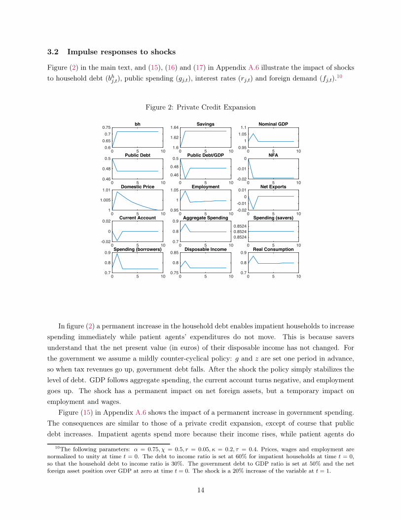
3.2 Impulse responses to shocks

Figure (2) in the main text, and (15), (16) and (17) in Appendix A.6 illustrate the impact of shocks

to household debt (bhj,t), public spending (gj,t), interest rates (rj,t) and foreign demand (fj,t).10

Figure 2: Private Credit Expansion

0 5 100.6

0.650.7

0.75bh

0 5 101.6

1.62

1.64Savings

0 5 100.95

11.05

1.1Nominal GDP

0 5 100.46

0.48

0.5Public Debt

0 5 100.46

0.48

0.5Public Debt/GDP

0 5 10-0.02

-0.01

0NFA

0 5 101

1.005

1.01Domestic Price

0 5 100.95

1

1.05Employment

0 5 10-0.02-0.01

00.01

Net Exports

0 5 10-0.02

0

0.02Current Account

0 5 100.7

0.8

0.9Aggregate Spending

0 5 10

0.85240.85240.8524

Spending (savers)

0 5 100.7

0.8

0.9Spending (borrowers)

0 5 100.75

0.8

0.85Disposable Income

0 5 100.7

0.8

0.9Real Consumption

In figure (2) a permanent increase in the household debt enables impatient households to increase

spending immediately while patient agents’ expenditures do not move. This is because savers

understand that the net present value (in euros) of their disposable income has not changed. For

the government we assume a mildly counter-cyclical policy: g and z are set one period in advance,

so when tax revenues go up, government debt falls. After the shock the policy simply stabilizes the

level of debt. GDP follows aggregate spending, the current account turns negative, and employment

goes up. The shock has a permanent impact on net foreign assets, but a temporary impact on

employment and wages.

Figure (15) in Appendix A.6 shows the impact of a permanent increase in government spending.

The consequences are similar to those of a private credit expansion, except of course that public

debt increases. Impatient agents spend more because their income rises, while patient agents do

10The following parameters: α = 0.75,χ = 0.5, r = 0.05, κ = 0.2, τ = 0.4. Prices, wages and employment arenormalized to unity at time t = 0. The debt to income ratio is set at 60% for impatient households at time t = 0,so that the household debt to income ratio is 30%. The government debt to GDP ratio is set at 50% and the netforeign asset position over GDP at zero at time t = 0. The shock is a 20% increase of the variable at t = 1.

14

not change their nominal spending and nominal interest rates in the small open economy do not

change. Prices are permanently higher in the long run. Figures (2) and (15) show the response

of the economy to two types of autonomous spending: that of constrained agents, and that of the

government. The spending multipliers are increasing functions of αi and χi. A higher share of

impatient agents in the economy implies that an increase in disposable income has a larger impact

on aggregate expenditures. A higher share of spending on domestic goods reduces leakage through

imports. Figure (16) in Appendix A.6 shows the response to an increase in domestic interest

rates.11 It induces patient households to save more, so it reduces their expenditures and generates a

recession (fall in nominal GDP and in employment) that forces impatient households to reduce their

spending. Imports fall and the net foreign asset position improves. Because of lower tax revenues,

the recession increases public debt. Figure (17) in the Appendix shows that an increase in foreign

demand permanently increases nominal GDP. Spending of both patient and impatient households

increase. The net foreign asset position improves. Public debt falls because of higher tax revenues.

4 Reduced Form Model

We simulate 11 eurozone countries from 2000 to 2012: Austria, Belgium, Germany, Spain, Finland,

France, Greece, Ireland, Italy, Netherlands and Portugal and calibrate the shocks on the observed

data. The data sources are described in Appendix B.1.

4.1 Calibration

The parameters used in the simulations are presented in Table (1). The discount factor (of patient

households) and the Philipps curve parameter are standard. The country-specific parameters – the

share of credit constrained households (χj) and the domestic share of consumption (αj) – are shown

on Figure (3).

Table 1: ParametersParameter Name ValueAnnual discount factor (patient) β 0.98Domestic share of consumption αj country specificShare of credit constrained households χj country specificPhillips curve parameter κ 0.3Persistence of spreads shocks θ 0.5

Trade: For the country specific domestic share of consumption, αj , we rely on Bussiere et al.

(2011) who compute the total import content of consumption expenditures, including the value

11For these impulse response functions we assume an iid process for the spread shock. However, for simulationswe use an AR process with the estimated persistence parameter θ.

15

of indirect imports. For our sample of countries the average implied domestic share in 2005 (the

latest date in their study) is 72.7%. The lowest is 66.4% for Belgium and the highest is 78.7% for

Italy. For foreign demand Fj,t, given the absence of an intermediate goods sector in our model, we

take the domestic value added that is associated with final consumption in the rest of the world,

which corresponds to value added based exports. As detailed in Appendix B.1, we use the data

from the OECD-WTO Trade in Value-Added (TiVA) initiative to measure this. The scaled value-

added based exports are shown in figure (26) in Appendix B.3. Finally, we take into account net EU

transfers, which are the difference between EU spending in the country and the country contribution

to the EU. In our model, such transfers play exactly the same role as foreign demand, so we add

EU net transfers to exports in the goods market equation.

Figure 3: Share of credit constrained households (χj) and domestic share of consumption (αj)

AUT

BEL

DEU

ESP

FIN

FRA

GRE

IRL

ITA

NLD

PRT

.6.6

5.7

.75

.8al

pha

.3 .4 .5 .6 .7chi

Share of Constrained Households: For the country specific share of credit constrained house-

holds, χj, we use a measure based on the Eurosystem Household Finance and Consumption Survey

(HFCS).12 For each country, we use the fraction of households with liquid assets below two months

of total household gross income to approximate the share of credit constrained households.13 The

12The survey took place in 2010. In Greece and Spain, the data were collected in 2009 and 2008-09 respectively.This survey has been used recently by Kaplan et al. (2014) to quantify the share of hand-to-month households. Theydefine these as consumers who spend all of their available resources in every pay-period, and hence do not carryany wealth across periods. They argue that measuring this behavior using data on net worth (as consistent withheterogeneous-agent macroeconomic models) is misleading because this misses what they call the wealthy hand-to-mouth households. These are households who hold sizable amounts of wealth in illiquid assets (such as housing orretirement accounts), but very little or no liquid wealth, and therefore consume all of their disposable income everyperiod. They define hand-to-mouth consumers as those households in the survey whose average balances of liquidwealth are positive but equal to or less than half their earnings.

13We thank Caterina Mendicino from the ECB who provided us the data. At the eurozone level, the medianhousehold has 18.6% of its annual income (equivalent to just above two months’ income) available in the form of

16

average for our set of countries is 48% with a maximum of 64.8% for Greece and a minimum of

34.7% for Austria. Ireland did not participate in the survey so for this country we use the average

of the eurozone. Note that bhj,t in the model is debt per impatient household so the counterpart to

the empirical measure of aggregate debt is χjbhj,t.

Funding Costs: The cost of fund ρj,t enters the Euler equation of unconstrained agents. It

represents the expected return of savers, the funding cost of firms, etc. The true cost of funds is not

directly observable and we base our estimates on several interest rates: (i) loans rates for SMEs; (ii)

deposit rates; (iii) wholesale bank funding costs; and (iv) yields on 10-year government bonds. In

all cases we compute the difference between the rate in country j and the median of the eurozone

in year t.

The link between interest rate spreads and funding costs can be complicated. On the one hand,

interest rates are not expected returns because they include expected credit losses. On the other

hand, we know from a large literature in finance that credit spreads create significant differences in

funding costs. This is the basic point of all models with distress costs, agency costs, debt overhang,

safety premia, etc. All these models predict that funding costs are increasing in credit spreads, but

less than one-for-one. Banks clearly play a special role during the crisis. Many borrowers depend

on bank loans and the funding costs of banks are therefore critical for the economy. We use data

on banks CDSs to estimate wholesale funding costs. Deposit rates are also informative even though

they tend to move more slowly than market rates. They also depend on the credibility of the deposit

insurance system. Debt overhang in the banking sector makes it more attractive for banks to invest

in the debt of their home sovereign, and this can crowd out private lending.14

We want our synthetic measure to be as broad as possible, so ideally we want to use the average

of (i) loans rates for SMEs; (ii) deposit rates; (iii) wholesale bank funding costs. Unfortunately we

are severely constrained by data availability, as explained in Appendix B.1. The only series that are

available for all countries and all years are the spreads on government bonds. We therefore project

our three spreads (SME loans, deposits, wholesale funding) on the sovereign spreads and we take

the average of the projected values.15

ρj,t ≡1

3

)

ˆSMEj,t + ˆDEPOj,t + ˆWHOLEj,t

*

.

Figure (27) in Appendix B.3 shows the government bond spreads and our synthetic measure ρj,t.

They are of course strongly correlated, but the important point is that ρj,t is a lot less volatile than

the government spread. In the case of Greece for instance, the sovereign spreads exceeds 20% in

liquid assets (see ECB-HFCS (2013)). Net liquid assets are the sum of deposits, mutual funds, bonds, non selfemployment business wealth, (publicly traded) shares and managed accounts, net of credit line/overdraft debt, creditcard debt and other non mortgage debt

14In the limit of a model à la Myers (1977), the bank may end up treating the entire yield as an expected returnbecause it only cares about the non-default state. See Philippon and Schnabl (2013) for a discussion of debt overhang.

15We regress each of the country specific interest spreads (loans for SMEs, deposit rates and wholesale bankfunding costs captured by CDS rates) on a piecewise linear function of the 10-year government bonds spread. Wethen take the simple average of the predicted values.

17

some years, and this is clearly a reflection of credit risk. Using this raw number in the simulations

would make no sense and would lead to too much volatility in spending. As we show below, our

synthetic measure seems to perform reasonably well in the simulations.

Finally, agents in our model need to have an estimate of the persistence parameter θ for the

ρj,t series. A higher persistence amplifies the effect of a given spread shock because it increases its

impact on the net present value of future income. It is clearly important to use a longer sample to

estimate the persistence so we extend all our spreads series to 2014 and we estimate θ by running

a panel regression with year and country fixed effects. We estimate θ to be 0.5, which means that

if the spread is 100bps this year, agents anticipate that it will be 50bps next year.

Scaling: We scale the data in a manner consistent with equation (13). We construct the following

benchmark level of nominal GDP for country j at time t:

Yj,t ≡Yj,t0

Lj,t0

Lt0

Yt0

Yt

LtLj,t,

where t0 is the base year (2002 in our simulations), Yj,t is GDP, Lj,t is population, and Yt and Lt

denote the aggregate GDP and population for the eurozone. In words, the benchmark is the nominal

GDP the country would have if it had the same per-capita growth rate as the eurozone together with

its actual population growth. The key point is that the only country level time-varying variable that

we take as exogenous is population growth. We scale all our variables in euros by the benchmark

GDP. For GDP itself, we define

yj,t ≡Yj,t

Yj,t

,

which is one in the base year. For sovereign debt, we define

bgj,t ≡Bg

j,t

Yj,t

,

which is equal to the actual debt to GDP ratio in the base year t0, but then tracks the level of debt

for t > t0, as in the model. This is important when we consider deleveraging. With large fiscal

multipliers, a reduction in debt might leave the debt to GDP ratio unchanged in the short run. Ratios

often give a misleading view of deleveraging efforts. Figure (24) in Appendix B.3 shows the scaled

private and sovereign debt series. Figure (25) shows scaled public spending and transfers. Note also

that government spending is adjusted for expenditures on bank recapitalization. Prices and wages

are the same in our model so we use the average of unit labor costs and consumer prices scaled by the

average unit labor cost and consumer prices in the eurozone. For employment, we use employment

per capita in deviation to the eurozone average and the base year: ni,t =Nj,t/Lj,t

Nj,2002/Lj,2002

N∗j,2002/L

∗j,2002

N∗j,t/L

∗j,t

.

18

4.2 Reduced Form Simulations

In our business cycle accounting exercise we take as given the observed series for private debt (bhj,t),

fiscal policy (gj,t, zj,t, τj) and interest rate spreads (ρj,t). We define the reduced form model ℜ as a

mapping

ℜ :)

bhj,t, gj,t, zj,t, ρj,t*

−→)

bgj,t, yj,t, nj,t, pj,t, ej,t, ..*

. (15)

The scaled data on observed shocks that feed the model for each country are shown in figures (24),

(25), (26) and (27) in Appendix B.3. For each country, we simulate the path between 2001 and

2012 of nominal GDP yj,t, employment nj,t, wages wj,t, net exports ej,t and public debt bgj,t. Figure

(4) shows the simulated and observed nominal GDP and net exports series. Figures (18) and (19)

in Appendix A.7 show employment and wages.

Figure 4: Reduced Form Model, Nominal GDP and Net ExportsGDP Net Exports

2001 2004 2008 2012

1

1.2

AUT

2001 2004 2008 2012

1

1.2

BEL

2001 2004 2008 2012

1

1.2

DEU

2001 2004 2008 2012

1

1.2

ESP

2001 2004 2008 2012

1

1.2

FIN

2001 2004 2008 2012

1

1.2

FRA

2001 2004 2008 2012

1

1.2

GRE

2001 2004 2008 2012

1

1.2

IRL

2001 2004 2008 2012

1

1.2

ITA

2001 2004 2008 2012

1

1.2

NLD

2001 2004 2008 2012

1

1.2

PRT

year

data

reduced form model

2001 2004 2008 2012

−0.10

0.10.2

AUT

2001 2004 2008 2012

−0.10

0.10.2

BEL

2001 2004 2008 2012

−0.10

0.10.2

DEU

2001 2004 2008 2012

−0.10

0.10.2

ESP

2001 2004 2008 2012

−0.10

0.10.2

FIN

2001 2004 2008 2012

−0.10

0.10.2

FRA

2001 2004 2008 2012

−0.10

0.10.2

GRE

2001 2004 2008 2012

−0.10

0.10.2

IRL

2001 2004 2008 2012

−0.10

0.10.2

ITA

2001 2004 2008 2012

−0.10

0.10.2

NLD

2001 2004 2008 2012

−0.10

0.10.2

PRT

year

data

reduced form model

The reduced form model reproduces well the cross sectional dynamics in the eurozone for nominal

GDP and net exports. In particular, it replicates well the boom and bust dynamics on nominal

GDP and the current account reversal for countries hit by the crisis. It is important to emphasize

that there is essentially no degree of freedom in our simulations. No parameter is set to match the

aggregate data. The model is entirely constrained by observable micro estimates and by equilibrium

conditions. The only parameter that we can adjust is the slope of the Phillips curve κ but it does

not affect the nominal GDP in euro, it only pins down the allocation of nominal GDP between

prices and quantities (employment).

It is nonetheless important to focus on the errors made by the model. There are three main

simulations errors. One is that the model over-predicts the boom/bust cycle in Greece. We think

that one reason might be that the increase in government spending took the form of higher wages

19

to public servants. To the extent that these agents are not credit constrained, our model can over-

estimate the departures from Ricardian equivalence. The second issue is the timing of Irish net

exports. The data seem to lag the model by one year. We are not quite sure why this is the case,

and this issue will appear again in our structural simulations. The third issue is in fact a good sign:

in Germany, the model fails to account the increase in the natural rate of employment following the

Hartz reforms of 2003-2005. We think this should show up as a change in the Phillips curve, and it

does.

5 Structural Model

Private leverage, spreads and fiscal policy are interrelated and our goal in this section is to identify

the structural relations between the three variables. We think of country dynamics as being driven

by three structural shocks. The first one is a boom/bust cycle in private debt, which we call credit

cycle for short. The second one is a political economy bias in government spending that creates

fiscal imbalances. The third is a sudden stop that threatens the stability of the eurozone. Formally,

we think of the structural model ℑ as a mapping

ℑ : (Credit Cycle, Political Economy, Sudden Stop) −→)

bhj,t, gj,t, ρj,t, yj,t, ...*

(16)

The key point of the structural model is to explain the variables that we took as exogenous in the

reduced form model (15). Our identification strategy is based on a mix of theoretical modeling and

empirical identification using instrumental variables. We do not claim to provide micro-foundations

for every detail of the model. Given the range of data and economic forces that we need to capture,

this is not feasible. But we mean that, either there is an explicit theoretical equation, or there is an

empirical equation that allows us to identify the influence of one variable on the others.

5.1 Using the U.S. to Identify Private Debt Dynamics

A serious identification challenge is to figure out how private deleveraging would play out if without

sudden stops. It is clear that there would be some deleveraging in any case, but exactly how fast

and how much, we do not know. It is also rather intuitive that places that experience the largest

increase in debt during the boom experience the largest decrease during the bust. This makes it

particularly difficult to come up with plausible instruments. Our identification strategy is then

to use the United States as a control group to estimate deleveraging without sudden stops. We

estimate the following model for deleveraging in a panel of U.S. states

bh,USj,t = α1b

h,USj,t−1 +

+

k=2002,2005,2008

αkbh,USj,k + ϵj,t

20

for t = 2009, .., 2012, j = 1, ..52, and bhj,t is household debt in state j at time t, rescaled exactly

as explained above for the eurozone.16 The idea is that these private leverage cycles reflect various

global and financial factors: low real rates, financial innovations, regulatory arbitrage of the Basel

rules by banks, real estate bubbles, bank governance, etc.17 To a large extent these forces were

present both in Europe and in the US. The difference of course is that there was no sudden stops

within the US. Hence, we interpret the US experience as representative of a deleveraging outcome in

a monetary union without sudden stops.18 The estimated coefficients αUSk are negative, capturing

the fact that states that accumulate more private debt during the boom deleverage more during the

bust. We then take the estimated coefficients αk and use them to construct predicted deleveraging

in eurozone countries:

bhj,t = α1bh,j,t−1 +

+

k=2002,2005,2008

αkbh,j,k

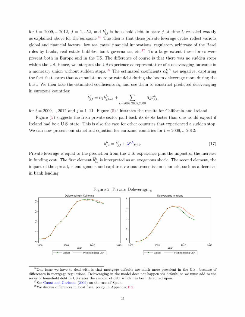
for t = 2009, .., 2012 and j = 1..11. Figure (5) illustrates the results for California and Ireland.

Figure (5) suggests the Irish private sector paid back its debts faster than one would expect if

Ireland had be a U.S. state. This is also the case for other countries that experienced a sudden stop.

We can now present our structural equation for eurozone countries for t = 2009, .., 2012:

bhj,t = bhj,t + λρ,hρj,t. (17)

Private leverage is equal to the prediction from the U.S. experience plus the impact of the increase

in funding cost. The first element bhj,t is interpreted as an exogenous shock. The second element, the

impact of the spread, is endogenous and captures various transmission channels, such as a decrease

in bank lending.

Figure 5: Private Deleveraging

.81

1.2

1.4

1.6

2000 2005 2010 2015year

Actual Predicted using USA

Deleveraging in California

.6.8

11.

21.

4

2000 2005 2010 2015year

Actual Predicted using USA

Deleveraging in Ireland

16One issue we have to deal with is that mortgage defaults are much more prevalent in the U.S., because ofdifferences in mortgage regulations. Deleveraging in the model does not happen via default, so we must add to theseries of household debt in US states the amount of debt which has been defaulted upon.

17See Cunat and Garicano (2009) on the case of Spain.18We discuss differences in local fiscal policy in Appendix B.2.

21

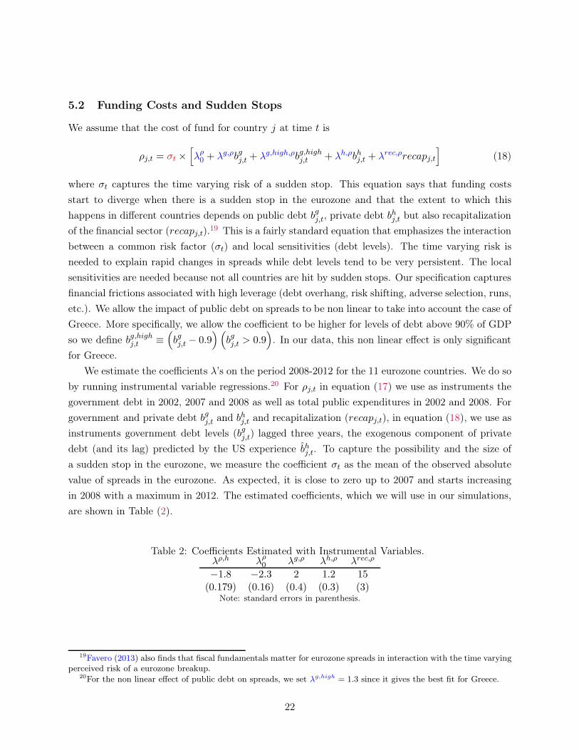
5.2 Funding Costs and Sudden Stops

We assume that the cost of fund for country j at time t is

ρj,t = σt ×,

λρ0 + λg,ρbgj,t + λg,high,ρbg,highj,t + λh,ρbhj,t + λrec,ρrecapj,t

-

(18)

where σt captures the time varying risk of a sudden stop. This equation says that funding costs

start to diverge when there is a sudden stop in the eurozone and that the extent to which this

happens in different countries depends on public debt bgj,t, private debt bhj,t but also recapitalization

of the financial sector (recapj,t).19 This is a fairly standard equation that emphasizes the interaction

between a common risk factor (σt) and local sensitivities (debt levels). The time varying risk is

needed to explain rapid changes in spreads while debt levels tend to be very persistent. The local

sensitivities are needed because not all countries are hit by sudden stops. Our specification captures

financial frictions associated with high leverage (debt overhang, risk shifting, adverse selection, runs,

etc.). We allow the impact of public debt on spreads to be non linear to take into account the case of

Greece. More specifically, we allow the coefficient to be higher for levels of debt above 90% of GDP

so we define bg,highj,t ≡)

bgj,t − 0.9* )

bgj,t > 0.9*

. In our data, this non linear effect is only significant

for Greece.

We estimate the coefficients λ’s on the period 2008-2012 for the 11 eurozone countries. We do so

by running instrumental variable regressions.20 For ρj,t in equation (17) we use as instruments the

government debt in 2002, 2007 and 2008 as well as total public expenditures in 2002 and 2008. For

government and private debt bgj,t and bhj,t and recapitalization (recapj,t), in equation (18), we use as

instruments government debt levels (bgj,t) lagged three years, the exogenous component of private

debt (and its lag) predicted by the US experience bhj,t. To capture the possibility and the size of

a sudden stop in the eurozone, we measure the coefficient σt as the mean of the observed absolute

value of spreads in the eurozone. As expected, it is close to zero up to 2007 and starts increasing

in 2008 with a maximum in 2012. The estimated coefficients, which we will use in our simulations,

are shown in Table (2).

Table 2: Coefficients Estimated with Instrumental Variables.λρ,h λρ

0 λg,ρ λh,ρ λrec,ρ

−1.8 −2.3 2 1.2 15(0.179) (0.16) (0.4) (0.3) (3)

Note: standard errors in parenthesis.

19Favero (2013) also finds that fiscal fundamentals matter for eurozone spreads in interaction with the time varyingperceived risk of a eurozone breakup.

20For the non linear effect of public debt on spreads, we set λg,high = 1.3 since it gives the best fit for Greece.

22

5.3 Fiscal Policy

Our last task is to specify a fiscal policy function for the different governments. We assume that the

government seeks to stabilize employment but is constrained by its cost of funds. The government

cuts spending when ρj,t is positive.21 We allow the funding constraint to have a stronger impact

for higher levels of the rescaled spreads (above 100 basis points): ρhighj,t ≡ max (ρj,t − 0.01, 0). This

non linear effect is important for Greece and to a lesser extent for Portugal. Hence, the policy rule

for government spending, with parameters γn, γρ and γρ,high, is given by:

gj,t = gj,t + γn (nj,t − n) + γρρj,t + γρ,highρhighj,t , (19)

zj,t = zj,t + γn (nj,t − n) + γρρj,t + γρ,highρhighj,t ,

where gj,t and zj,t are country specific drifts,

gj,t = gj,0 + δgj (min(t, t1)− t0)− δgj max (t− t1, 0) , (20)

zj,t = zj,0 + δzj (min(t, t1)− t0)− δzj max (t− t1, 0) ,

with t0 = 2002 and t1 = 2008. Hence, δgj represents the average “excess” annual spending growth

rate during the boom years. We interpret this drift as a political bias in spending decisions that is

reversed after 2008.22 What matters for us is that countries display different degrees of spending

bias during the boom years, and we want to analyze to what extent this spending drift during the

boom years contributes to the crisis.

Table 3: Fiscal policy coefficientsγn γρ γρ,high

−0.8 −2.5 −1.0

Table 4: Biases in government spendingδgj δzj

Spain Greece Ireland Portugal Spain Greece Ireland Portugal1.5% 0% 0.5% 0% 1.0% 3.5% 2.0% 0%

21In fact we use the lagged spread simply because it fits better, which probably reflects implementation lags infiscal policy. This is not related to the identification of the model and our results are not sensitive to this detail.

22The fact that it is reversed is not very important for our results. We could assume that gj,t stays constantafter t1 and our simulations would be similar. In fact, our counter-factual results would be stronger since the modelwould then choose a larger γρ to fit the data. But this can create issues of debt sustainability if we simulate themodel beyond 2012 and we assume that the spreads normalize. In practice we also see that governments are tryingto reverse some of the spending decisions they made during the boom years. The change in political bias might comefrom new fiscal rules agreed at the EU level, from explicit requirements for countries in a program, or more broadlyfrom a shift in attitudes and beliefs about fiscal responsibility

23

We focus on the four countries that are most harshly hit by the crisis, namely Spain, Greece,

Ireland and Portugal. We choose our parameters in the policy rule γn andγρ and the spending

and transfer drift coefficients δgj and δzj such that the model reproduces dynamics of public debt

(equivalently, spending and net taxes) during the boom. This leads us to the parameters given

in Tables (3) and (4). The spending biases necessary to reproduce the debt dynamics is larger in

Greece than in the other periphery countries. It is intermediate in Ireland and Spain and null in

Portugal. In Greece, the fiscal drift is entirely in the form of transfers reflecting the high growth

rate of wages in the public sector and the impact of the pension system in the boom years (see

Fernández Villaverde et al. (2013)). Finally, we need to take into account the Greek debt restruc-

turing. Greece benefits from low interest rates, extended repayment periods for the EU and IMF

rescue package, and a large reduction of outstanding debt. Altogether, we estimate that this is

equivalent to a decrease of 50 points of GDP, mostly in 2012.

Table 5: : Goodness of fit, structural modelESP GRE IRL PRT

yj,t 0.87 0.61 0.78 0.39nj,t 0.95 0.62 0.92 0.50pj,t 0.95 0.23 0.73 0.74bgj,t 0.93 0.95 0.94 0.92

ρj,t 0.90 0.87 0.98 0.82ej,t 0.80 0.70 0.2 0.75

Note: Goodness of fit is the share of variance explained by the model. It is measured as 1 − rssj/tssjwhere tssj is the total sum of squares and rssj is the residual sum of squares. For instance, for GDP, wehave tssj ≡

!2012t=2001 (yj,t − yj)

2, where yj,t and yj are the actual GDP and its sample mean, and rssj ≡

!2012t=2001

"

yj,t − yj,t + ¯yj − yj#2

, where yj,t is the prediction of the model and ¯yj its sample mean.

5.4 Fit of the structural model

The structural model is a constrained version of the reduced form model presented earlier. We can

now formally write equation (16) as

ℑ :)

bhj,t; δgj , δ

zj ;σt

*

−→)

bhj,t, gj,t, zj,t, ρj,t; bgj,t, yj,t, nj,t, pj,t, ej,t, ..

*

(21)

subject to the equilibrium condition of the model and the structural equations (17), (18) and (19).

There are three sets of exogenous factors: the fiscal biases δgj and δzj , the predicted private credit

cycle bhj,t, and the sudden stop shock σt.

24

Figure 6: Structural Model, Nominal GDP and EmploymentGDP Employment

2001 2004 2008 2012

0.9

0.95

1

1.05

1.1

1.15

1.2

ESP

2001 2004 2008 2012

0.9

0.95

1

1.05

1.1

1.15

1.2

GRE

2001 2004 2008 2012

0.9

0.95

1

1.05

1.1

1.15

1.2

IRL

2001 2004 2008 2012

0.9

0.95

1

1.05

1.1

1.15

1.2

PRT

year

databenchmark model

2001 2004 2008 2012

0.85

0.9

0.95

1

1.05

1.1ESP

2001 2004 2008 2012

0.85

0.9

0.95

1

1.05

1.1GRE

2001 2004 2008 2012

0.85

0.9

0.95

1

1.05

1.1IRL

2001 2004 2008 2012

0.85

0.9

0.95

1

1.05

1.1PRT

year

databenchmark model

Figure 7: Structural Model, Government Debt and Funding CostsGovernment Debt Funding Costs

2001 2004 2008 2012

0.4

0.6

0.8

1

1.2

1.4

1.6

1.8ESP

2001 2004 2008 2012

0.4

0.6

0.8

1

1.2

1.4

1.6

1.8GRE

2001 2004 2008 2012

0.4

0.6

0.8

1

1.2

1.4

1.6

1.8IRL

2001 2004 2008 2012

0.4

0.6

0.8

1

1.2

1.4

1.6

1.8PRT

year

databenchmark model

2001 2004 2008 2012−0.02

0

0.02

0.04

0.06

0.08ESP

2001 2004 2008 2012−0.02

0

0.02

0.04

0.06

0.08GRE

2001 2004 2008 2012−0.02

0

0.02

0.04

0.06

0.08IRL

2001 2004 2008 2012−0.02

0

0.02

0.04

0.06

0.08PRT

year

databenchmark model

Figure (6) compares the actual and predicted series for nominal GDP and employment in the

four periphery countries.23 Figure (7) does the same for public debt and funding costs. The model

accounts well for the timing and amplitude of the boom and bust episodes. Table (5) reports the

23As with the reduced form figures, we add the difference between the mean of the data and the mean of thestructural model. The observed and predicted net exports are shown in figure (20) in Appendix A.7

25

goodness of fit of the structural model, defined as the share of the variance explained by the model.

The goodness of fit is a number between −∞ and 1. It is positive if the model helps reduce the

unexplained variance, and it is one if the model fits perfectly. The fit is good, but there are some

issues. The model over-predicts employment and nominal GDP in Greece during the boom (see the

discussion above for the reduced form case). There is some timing issues with Ireland. In Portugal,

funding costs are a bit low and the model misses the downward employment trend early in the

sample. But, overall, the goodness of fit makes us confident that we can use the model to perform

our counter-factual experiments.24

6 Counterfactual experiments

The goal of this section is to provide counterfactual simulations of what would happen to Greece,

Spain, Ireland and Portugal if they followed a different set of policies. We consider four counterfac-

tuals:

• fiscal policy: what happens with more conservative fiscal policies before 2008?

• macro-prudential policies: what happens with limits on private debt before 2008?

• monetary policy: what happens if ECB prevents the sudden stop in 2008?

• fiscal devaluation: what happens if these countries devalue in 2009?

For the counterfactual experiments, we use the structural equations (17), (18) and (19) with the

estimated coefficients discussed above. In all our experiments, we report on the same graph the

actual data and the predicted counter-factual series.25 The simulations generate series for public

debt, private debt, employment, nominal GDP, net exports and spreads on the period 2001-2012,

using debt in 2000 as an initial point.

6.1 Counterfactual with a more conservative fiscal policy in the boom

How would countries have fared if they had followed more conservative fiscal policies during the

boom? We answer this question by setting δgj and δzj equal to zero for the four periphery countries.

For Spain, Ireland and Portugal all the other benchmark parameters are left unchanged. For Greece,

we need to deal with the debt relief issue. Given that the counterfactual conservative fiscal policy

generates debt to GDP ratios much lower than in the data in 2011 and 2012, we assume that debt

relief would not have taken place. Hence, for Greece the counterfactual is the combination of a more

24It might be worth emphasizing that the fit is absolutely not mechanical. Recall that our model has no productivityshock, which means that we do not extract any information from the actual GDP series. Another important fact,that we do not have the space to discuss here, is that all these results change dramatically if we use the wrong series.The goodness of fit turns negative if we do not use Trade in Value-Added to estimate foreign demand shocks, or (evenworse) if we use the raw government spread as an estimate of ρ.

25The predicted series is defined as data + (structural model with counterfactual parameters - structural modelwith benchmark parameters).

26

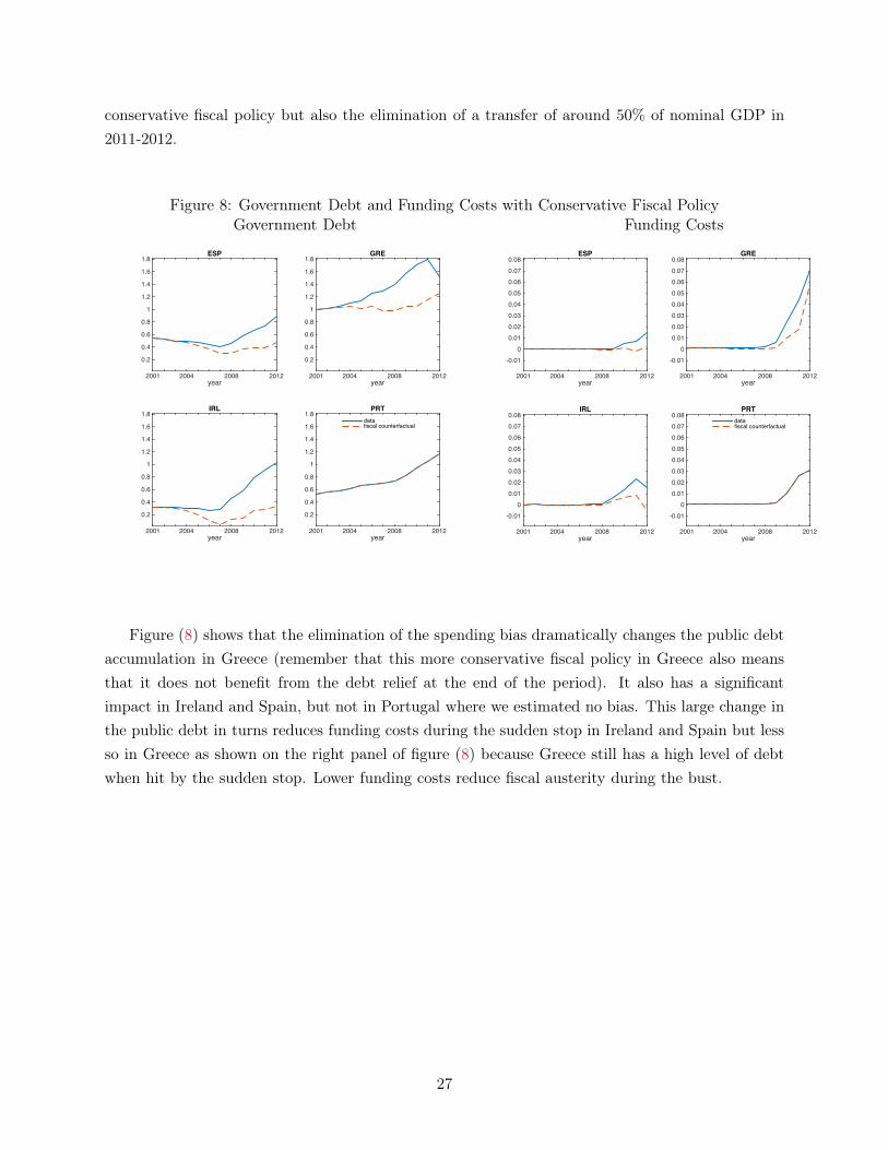
conservative fiscal policy but also the elimination of a transfer of around 50% of nominal GDP in

2011-2012.

Figure 8: Government Debt and Funding Costs with Conservative Fiscal PolicyGovernment Debt Funding Costs

year2001 2004 2008 2012

0.2

0.4

0.6

0.8

1

1.2

1.4

1.6

1.8ESP

year2001 2004 2008 2012

0.2

0.4

0.6

0.8

1

1.2

1.4

1.6

1.8GRE

year2001 2004 2008 2012

0.2

0.4

0.6

0.8

1

1.2

1.4

1.6

1.8IRL

year2001 2004 2008 2012

0.2

0.4

0.6

0.8

1

1.2

1.4

1.6

1.8PRT

datafiscal counterfactual

year2001 2004 2008 2012

-0.010

0.010.020.030.040.050.060.070.08

ESP

year2001 2004 2008 2012

-0.010

0.010.020.030.040.050.060.070.08

GRE

year2001 2004 2008 2012

-0.010

0.010.020.030.040.050.060.070.08

IRL

year2001 2004 2008 2012

-0.010

0.010.020.030.040.050.060.070.08

PRTdatafiscal counterfactual

Figure (8) shows that the elimination of the spending bias dramatically changes the public debt

accumulation in Greece (remember that this more conservative fiscal policy in Greece also means

that it does not benefit from the debt relief at the end of the period). It also has a significant

impact in Ireland and Spain, but not in Portugal where we estimated no bias. This large change in

the public debt in turns reduces funding costs during the sudden stop in Ireland and Spain but less

so in Greece as shown on the right panel of figure (8) because Greece still has a high level of debt

when hit by the sudden stop. Lower funding costs reduce fiscal austerity during the bust.

27

Figure 9: Employment with Conservative Fiscal Policy

year2001 2004 2008 2012

0.85

0.9

0.95

1

1.05

1.1ESP

year2001 2004 2008 2012

0.85

0.9

0.95

1

1.05

1.1GRE

year2001 2004 2008 2012

0.85

0.9

0.95

1

1.05

1.1IRL

year2001 2004 2008 2012

0.85

0.9

0.95

1

1.05

1.1PRT

datafiscal counterfactual

Figure (9) shows that a conservative fiscal policy allows Greece to stabilizes employment. The

actual employment loss of 15.8 percentage points (relative to the eurozone average) between 2008 and

2012 would have been almost halved with this more conservative fiscal policy. The counterfactual

conservative fiscal policies in Spain and Ireland do not eliminate the boom-bust cycle but allow for

an earlier exit from the recession, especially in Ireland. We have also checked that a counterfactual

with a pro-active fiscal adjustment reducing Portuguese public debt during the period 2001-2008

would have allowed Portugal to have a somewhat milder recession.

Finally, note that, in the counterfactual experiment, Ireland eliminates all public debt by the

end of the boom, and Spain reduces its public debt to around 30% of GDP. This does not seem very

realistic, and it suggests that fiscal policy is unlikely to be enough to stabilize an economy subject

to a large buildup of private debt. We therefore now turn to macro-prudential policies.

6.2 Counterfactual with macro-prudential policies in the boom

In this counterfactual we imagine that countries are able to prevent the private leverage boom. We

assume that bhj,t remains constant. We take into account the impact of such policy on the recapi-

talization of financial institutions during the bust: using a cross-sectional regression, we estimate

that a reduction of private debt by one euro during the boom reduces recapitalization needs by

0.25 euro during the bust. The macro-prudential policy in the boom therefore reduces public debt

and spreads. Figure (10) shows that this macro-prudential policy partially stabilizes employment

in all four countries. This is especially true in Ireland: whereas in the data employment falls from

2008 to 2012 by almost 12% more than the Eurozone average, in the counterfactual it falls by only

28

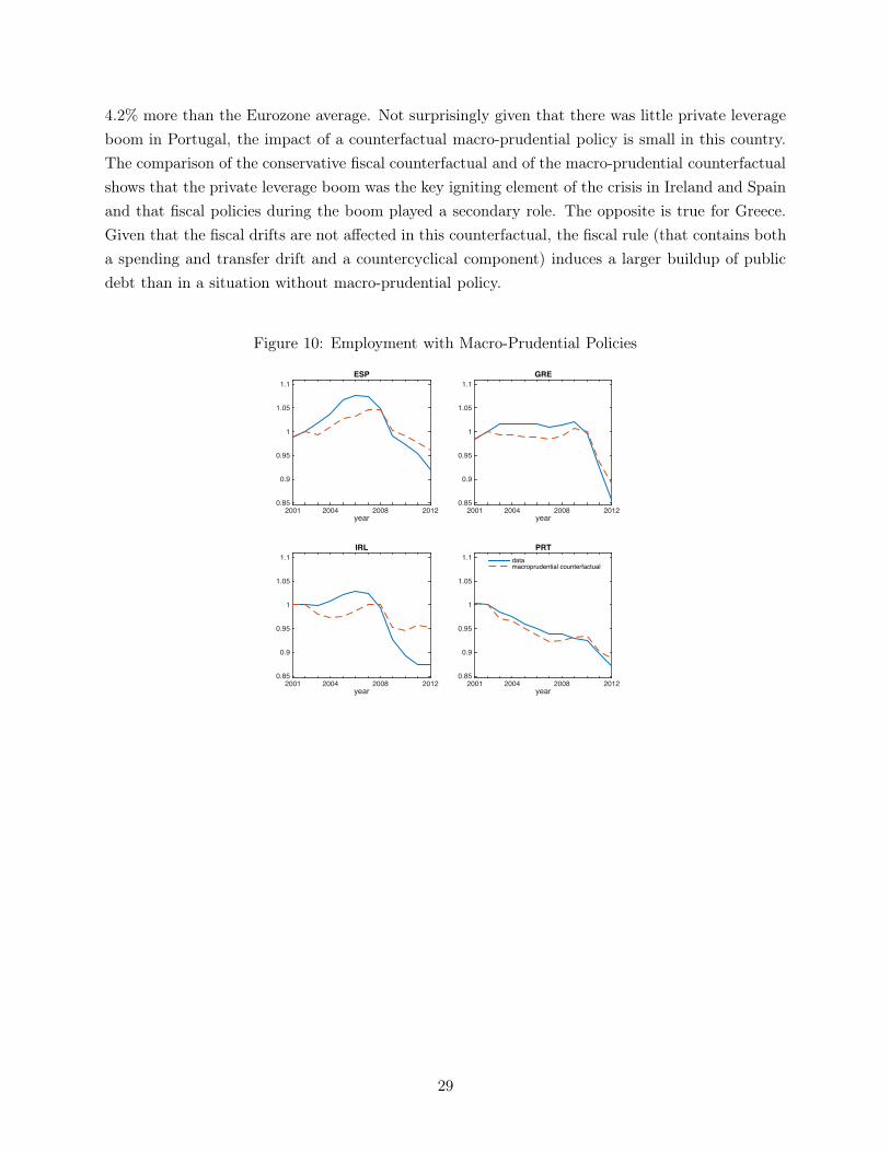
4.2% more than the Eurozone average. Not surprisingly given that there was little private leverage

boom in Portugal, the impact of a counterfactual macro-prudential policy is small in this country.

The comparison of the conservative fiscal counterfactual and of the macro-prudential counterfactual

shows that the private leverage boom was the key igniting element of the crisis in Ireland and Spain

and that fiscal policies during the boom played a secondary role. The opposite is true for Greece.

Given that the fiscal drifts are not affected in this counterfactual, the fiscal rule (that contains both

a spending and transfer drift and a countercyclical component) induces a larger buildup of public

debt than in a situation without macro-prudential policy.

Figure 10: Employment with Macro-Prudential Policies

year2001 2004 2008 2012

0.85

0.9

0.95

1

1.05

1.1ESP

year2001 2004 2008 2012

0.85

0.9

0.95

1

1.05

1.1GRE

year2001 2004 2008 2012

0.85

0.9

0.95

1

1.05

1.1IRL

year2001 2004 2008 2012

0.85

0.9

0.95

1

1.05

1.1PRT

datamacroprudential counterfactual

29

Figure 11: Government Debt and Funding Costs with Macro-Prudential PoliciesGovernment Debt Funding Costs

year2001 2004 2008 2012

0.4

0.6

0.8

1

1.2

1.4

1.6

1.8

2

ESP

year2001 2004 2008 2012

0.4

0.6

0.8

1

1.2

1.4

1.6

1.8

2

GRE

year2001 2004 2008 2012

0.4

0.6

0.8

1

1.2

1.4

1.6

1.8

2

IRL

year2001 2004 2008 2012

0.4

0.6

0.8

1

1.2

1.4

1.6

1.8

2

PRTdatamacroprudential counterfactual

year2001 2004 2008 2012

-0.010

0.010.020.030.040.050.060.070.08

ESP

year2001 2004 2008 2012

-0.010

0.010.020.030.040.050.060.070.08

GRE

year2001 2004 2008 2012

-0.010

0.010.020.030.040.050.060.070.08

IRL

year2001 2004 2008 2012

-0.010

0.010.020.030.040.050.060.070.08

PRTdatamacroprudential counterfactual

The public debt buildup in the boom can be seen in figure (11) in Spain, Greece and Ireland:

larger public debt is substituted to private debt to achieve the employment target. There are

two opposite effects on spreads: on the one hand the reduction in private leverage and in bank

recapitalization reduces spreads. On the other hand, the larger buildup of public debt pushes spreads

upward. In Ireland, the first effect clearly dominates as spreads disappear in this counterfactual

(see figure 11) largely because this counterfactual eliminates the need for bank recapitalization. In

the other three countries, this is not the case. This counterfactual suggests that macro-prudential

policies that do not come with a more prudent fiscal rule may not have been sufficient to generate a

fiscally sustainable stabilization of employment. In this sense, macro-prudential policies to constrain

private leverage and prudent fiscal policies to constrain public debt are complements not substitutes.

Indeed, we checked that in the case of Ireland and Spain, only a counterfactual that combines

prudent fiscal policies and macro-prudential policies succeeds in stabilizing both total debt and

employment.

6.3 Counterfactual with “whatever it takes” in 2008

In this counterfactual we ask the following question: what would have happened if the announce-

ments of July 2012 (Mario Draghi’s declaration “Whatever it takes”) and September 2012 (the OMT

program) had come earlier. These announcements were successful in reducing the risk of a euro

breakup, financial fragmentation and the sudden stop. The experiment is to imagine that these

actions were implemented and successful in 2008 rather than 2012. Specifically, we assume that σt,

30

the mean of the absolute value of spreads in the eurozone, in equation (18), is kept at its low 2007

level from 2008 on. This effectively eliminates (in Spain and Ireland) or strongly reduces (in Greece

and Portugal) the dramatic rise in funding costs as illustrated in figure (12).

Figure 12: Funding Costs with Early ECB Intervention

year2001 2004 2008 2012

-0.02-0.01

00.010.020.030.040.050.060.070.08

ESP

year2001 2004 2008 2012

-0.02-0.01

00.010.020.030.040.050.060.070.08

GRE

year2001 2004 2008 2012

-0.02-0.01

00.010.020.030.040.050.060.070.08

IRL

year2001 2004 2008 2012

-0.02-0.01

00.010.020.030.040.050.060.070.08

PRTdatano segmentation counterfactual

Figure 13: Employment and Government Debt with Early ECB InterventionEmployment Government Debt

year2001 2004 2008 2012

0.85

0.9

0.95

1

1.05

1.1ESP

year2001 2004 2008 2012

0.85

0.9

0.95

1

1.05

1.1GRE

year2001 2004 2008 2012

0.85

0.9

0.95

1

1.05

1.1IRL

year2001 2004 2008 2012

0.85

0.9

0.95

1

1.05

1.1PRT

datano segmentation counterfactual

year2001 2004 2008 2012

0.4

0.6

0.8

1

1.2

1.4

1.6

1.8ESP

year2001 2004 2008 2012

0.4

0.6

0.8

1

1.2

1.4

1.6

1.8GRE

year2001 2004 2008 2012

0.4

0.6

0.8

1

1.2

1.4

1.6

1.8IRL

year2001 2004 2008 2012

0.4

0.6

0.8

1

1.2

1.4

1.6

1.8PRT

datano segmentation counterfactual

31

The lower funding costs enable countries to stabilize employment (see figure 13). Interestingly,

the employment dynamics of Ireland then look similar to the ones of many U.S. states. There is a

large private leverage boom/bust cycle, but it is followed by a recovery starting in 2011. Finally,

although not stabilized, public debt is a bit lower than in the data as illustrated in figure (13). This

is due to larger fiscal receipts thanks to better GDP growth. Lower funding costs affect aggregate

spending and employment through three channels: 1) savers do not slash spending as much (see the

Euler equation 14); 2) the leverage of borrowers does not fall as much (see equation 17) which in

turn positively affects their spending; 3) fiscal austerity is reduced because fiscal policy (19) is less

constrained by the funding costs. We have checked that in all countries the fiscal channel is by far

the most important channel through which lower funding costs help stabilize employment.

6.4 Counterfactual with fiscal devaluation

In this counterfactual we ask the following question: what would have happened if periphery coun-

tries had been able to engineer a fiscal devaluation during the bust in order to recoup part of the

competitiveness they had lost during the boom years? This is close to a “flexible” exchange rate

counterfactual, but it is not identical because a fiscal devaluation does not impact the net foreign

asset position.26

Figure 14: Employment and Government Debt with Fiscal DevaluationEmployment Government Debt

year2001 2004 2008 2012

0.85

0.9

0.95

1

1.05

1.1

ESP

year2001 2004 2008 2012

0.85

0.9

0.95

1

1.05

1.1

GRE

year2001 2004 2008 2012

0.85

0.9

0.95

1

1.05

1.1

IRL

year2001 2004 2008 2012

0.85

0.9

0.95

1

1.05

1.1

PRTdatafiscal devaluation

year2001 2004 2008 2012

0.4

0.6

0.8

1

1.2

1.4

1.6

1.8ESP

year2001 2004 2008 2012

0.4

0.6

0.8

1

1.2

1.4

1.6

1.8GRE

year2001 2004 2008 2012

0.4

0.6

0.8

1

1.2

1.4

1.6

1.8IRL

year2001 2004 2008 2012

0.4

0.6

0.8

1

1.2

1.4

1.6

1.8PRT

datafiscal devaluation

26See Franco (2013) and Farhi et al. (2014) for conditions under which a fiscal devaluation is equivalent to anexchange rate adjustment.

32

More precisely, we assume that the fiscal devaluation is achieved through the combination of a

VAT tax on all domestic expenditures (private and public) and a payroll subsidy on wages. Appendix

A.8 details how the equilibrium conditions are amended. The VAT is paid by firms and rebated to

exporters. The payroll subsidy on labor is paid to domestic firms. To simplify further we assume

that the VAT rate and the payroll subsidy are equal to τv,j,t. Hence, export prices p∗j,t fall so foreign

demand increases to fj,t(1−τv,j,t)phj,t

due to unit elasticity, while domestic prices for domestic consumers

remain unchanged27. The fiscal devaluation is made fiscally neutral through a lump sum transfer

Γj,t to households such that:

Γj,t=τv,j,t(χjxb,j,t + (1− χj) xs,j,t + gj,t)− τv,j,twj,tnj,t

so that the revenues from the VAT equal the cost of the payroll subsidy and the transfer. However,

the indirect effects on income tax revenues that arise from the stimulative effects of a fiscal devalua-

tion on output remain as would be the case of an exchange rate devaluation. The fiscal devaluation

is applied starting in 2009. We set the VAT rate at 10% so that export volumes increase by the

same amount. The increase in exports attenuates the fall in employment in all countries as shown

in figure (14). Another effect of the fiscal devaluation is that the better employment figures induce

governments to cut spending and transfers. Because of this and because of the stimulative effect of

the fiscal devaluation on income taxes the trajectory of public debt is improved, as shown in figure

(14). This improvement in the debt dynamics is quite large in all countries: in 2012 public debt is

for example lower by around 20 percentage points of GDP in Ireland. This suggests that a condition

for a successful fiscal adjustment is that countries can benefit from such a change in relative prices.

In all countries, because of the reduction in public debt, funding costs are a bit lower.

7 Conclusion

Understanding the dynamics of the Eurozone is a major challenge for macroeconomics. Eurozone

countries have experienced extraordinary levels of real and financial volatility. Unemployment rates

have diverged to an extent that no one anticipated. While most observers recognize that private

leverage, fiscal policy, sudden stops and loss of competitiveness all played a role, it has proven

challenging to analyze them jointly, and even more difficult to disentangle them.

Our paper makes three contributions. We present a model that accounts simultaneously for

domestic credit, fiscal policy, and current account dynamics. We create a data set for 11 countries

over 13 years that covers the variables of interest and deals with the various accounting issues.

Finally, and most importantly, we propose a new identification strategy that allows us to run counter-

factual experiments regarding fiscal policy, macro-prudential policy, ECB interventions, and fiscal

devaluations. The results from our counter-factual experiments on employment are summarized

in Table 6. Stronger fiscal discipline during the boom would have made the recession less severe,

27Domestic prices and wages actually increase relative to data but only indirectly because of higher employment.

33

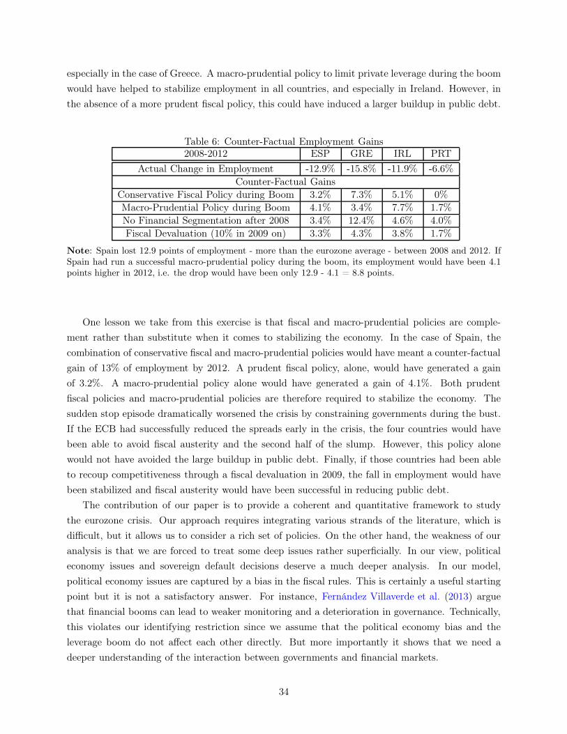
especially in the case of Greece. A macro-prudential policy to limit private leverage during the boom

would have helped to stabilize employment in all countries, and especially in Ireland. However, in

the absence of a more prudent fiscal policy, this could have induced a larger buildup in public debt.

Table 6: Counter-Factual Employment Gains2008-2012 ESP GRE IRL PRT

Actual Change in Employment -12.9% -15.8% -11.9% -6.6%Counter-Factual Gains

Conservative Fiscal Policy during Boom 3.2% 7.3% 5.1% 0%Macro-Prudential Policy during Boom 4.1% 3.4% 7.7% 1.7%No Financial Segmentation after 2008 3.4% 12.4% 4.6% 4.0%Fiscal Devaluation (10% in 2009 on) 3.3% 4.3% 3.8% 1.7%

Note: Spain lost 12.9 points of employment - more than the eurozone average - between 2008 and 2012. IfSpain had run a successful macro-prudential policy during the boom, its employment would have been 4.1points higher in 2012, i.e. the drop would have been only 12.9 - 4.1 = 8.8 points.

One lesson we take from this exercise is that fiscal and macro-prudential policies are comple-

ment rather than substitute when it comes to stabilizing the economy. In the case of Spain, the

combination of conservative fiscal and macro-prudential policies would have meant a counter-factual

gain of 13% of employment by 2012. A prudent fiscal policy, alone, would have generated a gain

of 3.2%. A macro-prudential policy alone would have generated a gain of 4.1%. Both prudent

fiscal policies and macro-prudential policies are therefore required to stabilize the economy. The

sudden stop episode dramatically worsened the crisis by constraining governments during the bust.

If the ECB had successfully reduced the spreads early in the crisis, the four countries would have

been able to avoid fiscal austerity and the second half of the slump. However, this policy alone

would not have avoided the large buildup in public debt. Finally, if those countries had been able

to recoup competitiveness through a fiscal devaluation in 2009, the fall in employment would have

been stabilized and fiscal austerity would have been successful in reducing public debt.

The contribution of our paper is to provide a coherent and quantitative framework to study

the eurozone crisis. Our approach requires integrating various strands of the literature, which is

difficult, but it allows us to consider a rich set of policies. On the other hand, the weakness of our

analysis is that we are forced to treat some deep issues rather superficially. In our view, political

economy issues and sovereign default decisions deserve a much deeper analysis. In our model,

political economy issues are captured by a bias in the fiscal rules. This is certainly a useful starting

point but it is not a satisfactory answer. For instance, Fernández Villaverde et al. (2013) argue

that financial booms can lead to weaker monitoring and a deterioration in governance. Technically,

this violates our identifying restriction since we assume that the political economy bias and the

leverage boom do not affect each other directly. But more importantly it shows that we need a

deeper understanding of the interaction between governments and financial markets.

34

Similarly, we summarize sovereign default risk by a bond pricing equation. We are of course

careful to estimate this equation with plausible instruments and to make sure that it fits well,

which is critical for our experiments. But this clearly is not a satisfactory treatment of strategic

sovereign default. Moreover, this approach does not help us to analyze reforms that would severe

the link between sovereign risk and the private cost of funds. A sensible goal for the eurozone is to

make sure that governments can default within the currency union and without destroying private

financial markets. Understanding what is required to reach this goal is an important avenue for

future research.

35

References

Accominotti, O. and B. Eichengreen (2013). The mother of all sudden stops: Capital flows andreversals in europe, 1919-1932. Berkeley Economic History Laboratory Working Paper 2013/7.

Aguiar, M. and G. Gopinath (2007). Emerging market business cycles: the cycle is the trend.Journal of Political Economy 115, 69–102.

Arellano, C. (2008). Default risk and income fluctuations in emerging economies. American Eco-nomic Review 98 (3), 690–712.

Battistini, N., M. Pagano, and S. Simonelli (2014, April). Systemic risk, sovereign yields and bankexposures in the euro crisis. Economic Policy 29 (78), 203 – 251.

Bernanke, B., M. Gertler, and S. Gilchrist (1999). The financial accelerator in a quantitativebusiness cycle framework. In J. B. Taylor and M. Woodford (Eds.), Handbook of Macroeconomics,Volume 1C. Elsevier Science, North Holland.

Bussiere, M., G. Callegari, F. Ghironi, G. Sestieri, and N. Yamano (2011). Estimating trade elas-ticities: Demand composition and the trade collapse of 2008-09. NBER Working Paper 17712.

Chari, V., P. Kehoe, and E. McGrattan (2005). Sudden stops and output drops. American EconomicReview Papers and Proceedings 95 (2), 381–387.

Chari, V. V., P. J. Kehoe, and E. R. McGrattan (2007, Oct). Business cycle accounting. Econo-metrica 75 (3), 781–836.

Christiano, Lawrence J., C. G. and J. Roldos (2004). Monetary policy in a financial crisis. Journalof Economic Theory 119, 1–245.

Cole, H. and M. Obstfeld (1991). Commodity trade and international risk sharing: How much dofinancial markets matter. Journal of Monetary Economics 28, 3–24.

Corsetti, G., K. Kuester, A. Meier, and G. J. Müller (2013). Sovereign risk, fiscal policy, andmacroeconomic stability. Economic Journal (123), 99 – 132.

Cunat, V. and L. Garicano (2009). Did good cajas extend bad loans? governance, human capitaland loan portfolios. FEDEA Monograph, "The Crisis of the Spanish Economy .

Cunat, V. and M. Guadalupe (2009). Executive compensation and competition in the banking andfinancial sectors. Journal of Banking and Finance 33, 439–474.

Eaton, J. and M. Gersovitz (1982). Debt with potential repudiation: Theoretical and empiricalanalysis. The Review of Economic Studies 48 (2), 289–309.

ECB-HFCS (2013, April). The eurosystem household, finance and consumption survey, results fromthe first wave. Statistics Paper Series 2, European Central Bank.

Eggertsson, G. and P. Krugman (2012). Debt, deleveraging, and the liquidity trap:a fisher-minsky-koo approach. Quarterly Journal of Economics (127(3)), 1469–1513.

Farhi, E., G. Gopinath, and O. Itskhoki (2014). Fiscal devaluations. Review of Economic Studies 81,725–760.

36

Farhi, E. and I. Werning (2013). Fiscal multipliers: Liquidity traps and currency unions.

Favero, C. (2013). Modelling and forecasting government bond spreads in the euro area: a gvarmodel. Journal of Econometrics 117 (2), 343–356.

Fernández Villaverde, J., L. Garicano, and T. Santos (2013). Political credit cycles: the case of theeurozone. Journal of Economc Perspectives 27 (3), 145–66.

Franco, F. (2013). Fiscal devaluation in portugal. Mimeo.

Gali, J. (2008). Monetary Policy, Inflation, and the Business Cycle. Princeton University Press.

Gali, J. and T. Monacelli (2008). Optimal monetary and fiscal policy in a currency union. Journalof International Economics 76, 116–132.

Gertler, M. and N. Kiyotaki (2010). Financial intermediation and credit policy in business cycleanalysis. Working Paper, NYU.

Giroud, X. and H. Mueller (2015). Firm leverage and unemployment during the great recession.mimeo NYU.

Gopinath, G. (2004). Lending booms, sharp reversals and real exchange rate dynamics. Journal ofInternational Economics 62, 1–23.

Gourinchas, P.-O. and M. Obstfeld (2012). Stories of the twentieth century for the twenty-first.American Economic Journal Macro 4 (1), 226–265.

Ivashina, V. and D. Scharfstein (2008). Bank lending during the financial crisis of 2008. HarvardBusiness School Working Paper.

Justiniano, A., G. Primiceri, and A. Tambalotti (2014). Credit supply and the housing boom.mimeo Northwestern.

Kaplan, G. and G. Violante (2011). A model of the consumption response to fiscal stimulus pay-ments. mimeo NYU.

Kaplan, G., G. L. Violante, and J. Weidner (2014). The wealthy hand-to-mouth. Working Paper.

Kiyotaki, N. and J. Moore (1997, Apr). Credit cycles. Journal of Political Economy 105 (2), 211–248.

Korinek, A. and E. G. Mendoza (2013). From sudden stops to fisherian deflation: Quantitativetheory and policy implications. NBER WP 19362.

Lane, P. (2012). The european sovereign debt crisis. Journal of Economic Perspectives 26 (3), 49–68.

Lane, P. (2013). Capital flows in the euro area. European Economy, Economic Papers 497.

Lee, D. and W. van der Klaauw (2012, November). An introduction to the frbny consumer creditpanel. Federal Reserve Bank of New York Staff Reports.

Mankiw, N. G. (2000). The savers-spenders theory of fiscal policy. American Economic ReviewPapers and Proceedings, 120–125.

Martin, P. and H. Rey (2006). Globalization and emerging markets: With or without crash?American Economic Review vol 96, n5, 1631–51.

37

Martinez, J. and T. Philippon (2014). Does a currency union need a capital market union? WorkingPaper, NYU.

Mendoza, E. G. (2010). Sudden stops, financial crises, and leverage. American Economic Re-view 100, 1941–1966.

Mendoza, E. G. and K. Smith (2006). Quantitative implications of a debt-deflation theory of suddenstops and asset prices. The Journal of International Economics Volume 70, Issue 1, 82–114.

Mendoza, E. G. and V. Z. Yue (2012). A general equilibrium model of sovereign default and businesscycles. The Quarterly Journal of Economics 127, 889–946.

Mian, A. and A. Sufi (2010). Household leverage and the recession of 2007-2009. IMF EconomicReview 1, 74–117.

Mian, A. and A. Sufi (2012). What explains high unemployment? the aggregate demand channel.Working Paper.

Midrigan, V. and T. Philippon (2010). Household leverage and the recession. NYU Working Paper.

Montoya, L. and B. Dohring (2011, October). The improbable renaissance of the phillips curve:The crisis and euro area inflation dynamics. European Commission Economic Paper.

Myers, S. C. (1977). Determinants of corporate borrowing. Journal of Financial Economics 5,147–175.

Nakamura, E. and J. Steinsson (2014). Fiscal stimulus in a monetary union: Evidence from u.s.regions. The American Economic Review .

Neumeyer, P. A. and F. Perri (2005). Business cycles in emerging economies: the role of interestrates. Journal of Monetary Economics 52 (2), 345–380.

Philippon, T. and P. Schnabl (2013, February). Efficient recapitalization. Journal of Finance 68 (1),1–42. NBER WP 14929.

Reis, R. (2013, Spring). The portuguese slump and crash and the euro crisis. Brookings Papers onEconomic Activity , 143–193.

Schmitt-Grohe, S. and M. Uribe (2012). Downward nominal wage rigidity, currency pegs, andinvoluntary unemployment. Working Paper.

Shambaugh, J. C. (2012, Spring). The euro’s three crises. Brookings Papers on Economic Activ-ity 212-219.

Whelan, K. (2014, March). Ireland’s economic crisis: The good, the bad and the ugly. Journal ofMacroeconomics.

38

A For Online Publication: Model and Simulation Appendix

A.1 Scaling

We have already defined the Euler equations for countryj and the monetary union (with an asterisk):

Et [Xs,j,t+1] ≈ β (1 + rj,t)Xs,j,t ; Et'

X∗s,t+1

(

≈ β.

1 + r∗s,t/

X∗s,t.

and the spread as

1 + ρj,t ≡1 + rj,t1 + r∗s,t

If we scale the budget constraint (assuming perfect foresight, or equivalently, neglecting the condi-tional variance of the aggregate shocks), we get

Xs,j,t

X∗s,t

+Sj,t+1

X∗s,t+1

X∗s,t+1

X∗s,t

1 + rj,t=

Sj,t

X∗s,t

+Yj,t

X∗s,t

and up to the usual approximation we have

xs,j,t +β

1 + ρj,tsj,t+1 = sj,t + yj,t

For the Phillips Curve we start from (12) and the equivalent equation at the eurozone level:

W ∗t

W ∗t−1

=

%

N∗t

N∗

&κ

.

Then we define

nj,t ≡Nj,t/Nj

N∗t /N

∗and wj,t ≡

Wj,t

W ∗j,t

.

To a first order approximation we then have

wj,t

wj,t−1= 1 + κ (nj,t − 1) .

Notice that this kind of log linear relation would hold even if the aggregate wage has a forwardlooking component so in fact we only need to assume that the country specific component follows(12).28 Since

nj,t =yj,twj,t

we have

(wj,t)2

wj,t−1+ (κ− 1)wj,t − κyj,t = 0

28In logs, we can write logWjt = logW ∗jt + logwjt. For the aggregate component we can then write: logW ∗

jt =ζEt logW

∗jt+1 + (1− ζ) logW ∗

jt−1 + κ∗$

logN∗t − log N∗

%

, where ζ captures the kind of hybrid Phillips curve thatmany people have estimated. In particular, our model is perfectly consistent with the idea that monetary policycan influence expected inflation at the aggregate level. We only assume that the country specific component follows:logwjt = logwjt−1 + κ log njt. We have also estimated a country specific forward looking component but found it tobe insignificant. For the sake of simplicity we therefore omit it.

39

Defining ∆ ≡ (κ− 1)2 + 4κ yj,twj,t−1

, we find that

wj,t

wj,t−1=

1− κ+√∆

2

Note that if yj,twj,t−1

= 1, then ∆ = (κ+ 1)2, and wj,t

w,t−1= 1.

A.2 Budget constraints

Let us first rewrite the budget constraints and market clearing conditions. Using the market clearingcondition, and competition phj,t = wj,t, we get

yj,t = αj (χjxb,j,t + (1− χj)xs,j,t) + fj,t + gj,t.

Nominal exports are fj,t, nominal imports are (1− χj) pfj,tc

fs,j,t + χjp

fj,tc

fb,j,t since the government

does not buy imported goods. So net exports are ej,t = fj,t − (1− αj) (χjxb,j,t + (1− χj)xs,j,t) .We define disposable (after-tax) income as yj,t ≡ (1− τj,t) yj,t + zj,t.

We can then write the system for nominal variables

• xb,j,t =β

1+ρj,tbhj,t+1 + yj,t − bhj,t, budget constraint of impatient agents

• xs,j,t = sj,t + yj,t − β1+ρj,t

sj,t+1, budget constraint of patient agents

• yj,t = αj (χjxb,j,t + (1− χj) xs,j,t) + fj,t + gj,t, market clearing

• gj,t + zj,t − τj,tyj,t =β

1+ρj,tbgj,t+1 − bgj,t, budget constraint of the government

• ej,t =1αj

(fj,t − (1− αj) (yj,t − gj,t)), definition of net exports

Combining the first four equations, we get market clearing at time t:

(1− αj) yj,t = αjχj

!

βbhj,t+1

1 + ρj,t− bhj,t

"

+αj (1− χj)

%

sj,t − βsj,t+1

1 + ρj,t

&

+βbgj,t+1

1 + ρj,t−bgj,t+fj,t. (22)

A.3 Pseudo-Steady State

We consider a steady state with constant interest rates equal to the rate of time preference ofsavers, i.e. β (1 + rj) = 1 and the spread is zero: ρj = 0. The borrowing limit bhj is exogenousand we consider equilibria where the borrowing constraint (4) binds. Our notion of steady state iscomplicated by the fact that savings sj are history-dependent. We define a steady state as the longrun equilibrium of an economy with initial savings sj and government debt bgj , subject to no furthershocks, constant government spending and constant government debt. All nominal quantities are

40

constant and employment is at its natural rate n.29 The long-run equilibrium conditions are

phj n = χjαjxb,j + (1− χj)αjxs,j + f + gj

xb,j = yj −r

1 + rbhj

xs,j = yj +r

1 + rsj

τjphj n = gj + zj +

r

1 + rbgj

Nominal output (the price of home goods) is pinned down by

phj n = αj

)

(1− τj) phj n+ zj

*

+ αjr

1 + r

.

(1− χj) sj − χj bj/

+ fj + gj .

There are several ways to specify government policy. Here we assume that the policy is to keepgovernment debt and nominal spending gj constant. Long run nominal output is then given by

phj n =αj

1− αjraj +

fj1− αj

+ gj (23)

where recall that we have defined a as net foreign assets. This equation shows the determinants ofthe long run price level. The long run price level depends on the exogenous components of spending:net asset income, foreign demand, and government spending. All these are inflationary. For a giventax rate τj, transfers are then chosen to satisfy the government’s budget constraint:

zj = τjphj n− gj −

r

1 + rbgj .

A.4 Euler Equation and Expected Income

We use a linear approximation of the Euler equation of savers:

Et [xs,j,t+1] = (1 + ρj,t) xs,j,t.

Consider the following experiment. Savers enter the period with a given level of savings. Then thereis a shock to interest rates. For instance, starting from a steady state where ρj = 0, if the new rateis such that ρj > 0, savings jumps up, and if the new rate is such that ρj < 0, spending jumps up.The budget constraint at time t is

xs,j,t = sj,t + yj,t − βsj,t+1

1 + ρj,t

and the expected budget constraint at time t+ 1 is

Et

#

βsj,t+2

1 + ρj,t+1

$

= sj,t+1 + Et [yj,t+1 − xs,j,t+1] .

Combining the budget constraints and the linearized Euler equation, we get

(1 + β)sj,t+1 + Et [yj,t+1]− Et

#

βsj,t+2

1 + ρj,t+1

$

= (1 + ρj,t) (sj,t + yj,t) . (24)

29We consider here the case where labor supply is inelastic, so n is effectively exogenous.

41

A.5 Equilibrium Conditions of the Model

We assume an AR(1) process for the spread:

• Et [ρj,t+1] = θρj,t, spreads

The equilibrium conditions are then

• Et [xs,j,t+1] = (1 + ρj,t) xs,j,t, Euler equation

• xb,j,t =β

1+ρj,tbhj,t+1 + yj,t − bhj,t, budget constraint of impatient agents

• xs,j,t = sj,t + yj,t − β1+ρj,t

sj,t+1, budget constraint of patient agents

• yj,t = αj (χjxb,j,t + (1− χj) xs,j,t) + fj,t + gj,t, market clearing

• gj,t + zj,t − τj,tyj,t = βbgj,t+1

1+ρj,t− bgj,t, budget constraint of the government

• ej,t =1αj

(fj,t − (1− αj) (yj,t − gj,t)), net exports

• yj,t = (1− τj) yj,t + zj,t, disposable income

• sj,t+1 = (1 + ρj,t) (sj,t + yj,t)−1−βθ(1+ρj,t)

1−βθ Et [yj,t+1], saving dynamics

• (1− αj) yj,t = αjχj

%

βbhj,t+1

1+ρj,t− bhj,t

&

+αj (1− χj))

sj,t − β sj,t+1

1+ρj,t

*

+βbgj,t+1

1+ρj,t−bgj,t+fj,t, market

clearing

•)

1− αj + αj

)

(1− χj)βθ

1−βθρj,t**

Et [yj,t+1] = (1− β))

αj (1− χj) sj,t+1 − αjχjbhj,t+1 − bgj,t+1

*

+

fj,t − θβρj,t)

αjχjbhj,t+1 + bgj,t+1

*

, expected market clearing

• nj,t =yj,twj,t

, labor market

• wj,t−wj,t−1

wj,t−1= κ (nj,t − nj), inflation

A.6 Impulse Response Functions

To compute the impulse response functions of the model we need to make an assumption about thepath of household debt and fiscal policy

Assumptions A1.

• Shocks on borrowing constraints are such that Et

,

bhj,t+2

-

= bhj,t+1.

• Fiscal policy is such that Et

,

bgj,t+2

-

= bgj,t+1 and the tax rate τj is constant.

• The variance of interest rates and foreign demand is small, and βb is small enough that bj,t =bhj,t at all times.

• Spreads are iid: Et [ρj,t+1] = 0. Savers anticipate spreads to last only one year.

42

Assumptions A1 are only necessary to solve for the entire path of macroeconomic variables shown inthe impulse response functions. The first condition says that shocks on borrowing are permanent.The second defines a class of fiscal policies. The third point is purely technical. It allows us tolinearize Euler equations. We assume that the shocks are small enough that impatient householdsfind it optimal to borrow up to the constraint (this is a joint restriction on the discount factor andthe size of the shocks). Note that the last assumption does not impose that the interest rate in themonetary union is iid, only that deviations for a particular country are expected to last one year.Assumptions A1 are not necessary for the reduced form and structural simulations.

We now look for decision rules for the savers {sj,t}t=1,2... and the other variables of the model,

yj,t, phj,t, etc. We get the following Lemma:

Lemma 1. Under A1 and Et [fj,t+1] = fj,t savings dynamics satisfy Et [sj,t+2] = sj,t+1.

Proof. We guess and verify that the Lemma is correct. Suppose the Lemma is true, then we obtaintwo important equations. Equation (24) becomes

sj,t+1 = (1 + ρj,t) (sj,t + yj,t)− Et [yj,t+1] , (25)

and expected market clearing at t+ 1 is

(1− αj)Et [yj,t+1] = (1− β))

αj (1− χj) sj,t+1 − αjχbhj,t+1 − bgj,t+1

*

+ fj,t. (26)

Therefore

(1− αj) sj,t+1 = (1− αj) (1 + ρj,t) (sj,t + yj,t)−(1− β))

αj (1− χj) sj,t+1 − αjχbhj,t+1 − bgj,t+1

*

−fj,t

1− αj.

Using market clearing at time t we get

sj,t+1

1 + ρj,t− sj,t =

αjχj

1− αjχj

!

bhj,t+1

1 + ρj,t− bhj,t

"

+1

1− αjχj

!

bgj,t+1

1 + ρj,t− bgj,t +

ρj,t1 + ρj,t

fj,t1− αj

"

(27)

Savings inherit the dynamic properties of bhj,t and bgj,t. Since we assume small shocks and Et [ρj,t+1] =0, this validates our conjecture that Et [sj,t+2] = sj,t+1.

Equilibrium conditions The five equilibrium conditions of the model with θ = 0 are

1. sj,t+1 = (1 + ρj,t) (sj,t + yj,t)− Et [yj,t+1]

2. (1− αj)Et [yj,t+1] = (1− β))

αj (1− χj) sj,t+1 − αjχjbhj,t+1 − bgj,t+1

*

+ fj,t.

3. (1− αj) yj,t = αjχj

%

bhj,t+1

1+rj,t− bhj,t

&

+ αj (1− χj))

sj,t − β sj,t+1

1+ρj,t

*

+ βbgj,t+1

1+ρj,t− bgj,t + fj,t.

4. gj,t + zj,t − τjyj,t = βbgj,t+1

1+ρj,t− bgj,t

5. yj,t = (1− τj) yj,t + zj,t

The five unknown endogenous variables are yj,t, yj,t, bgj,t, sj,t+1, and Et [yj,t+1]. The exogenous

shocks are bhj,t, fj,t and ρj,t. The policy shocks variables are transfers and public expenditure, zj,tand gj,t respectively. The state space of predetermined endogenous variables is sj,t and bgj,t.

43

We specify the policy function of the government in order to compute the impulse responses.We are interested in simple rules that deliver the property that the public debt follows a random

walk: Et

,

bgj,t+2

-

= bgj,t+1 and deliver some automatic stabilization. We assume that spending and

transfers are predetermined. From the government budget constraint, this means that a recessionat time t automatically increases government debt at time t. To maintain fiscal stability, we specify

that transfers adjust from t to t + 1 to keep public debt constant thereafter: Et

,

bgj,t+2

-

= bgj,t+1.

More precisely, we specify the general policy rule as follows

1. Fiscal variables gj,t and zj,t are pre-determined. Government debt bgj,t is determined in equi-librium at time t.

2. Set transfers zj,t+1 for next period so that Et

,

bgj,t+2

-

= bgj,t+1 assuming a martingale for gj,t.

(a) The expected budget constraint is

τjEt [yj,t+1] = gj,t + zj,t+1 + (1− β) bgj,t+1

(b) By definition we have

Et [yj,t+1] = (1− τj)Et [yj,t+1] + zj,t+1

(c) Therefore (recall that Et [yj,t+1] is part of our solution at time t), zj,t+1 is given by

zj,t+1 = τjEt [yj,t+1]− (1− τj) gj,t − (1− τj) (1− β) bgj,t+1

Figures (15), (16) and (17) illustrate the impulse response functions of the model for a shock tohousehold debt (bhj,t), public spending (gj,t), interest rates (rj,t) and foreign demand (fj,t) respec-tively.

Figure 15: Fiscal Expansion

0 5 100.2

0.22

0.24g

0 5 101.6

1.62

1.64Savings

0 5 101

1.021.041.06

Nominal GDP

0 5 100.5

0.51

0.52Public Debt

0 5 100.49

0.495

0.5Public Debt/GDP

0 5 10

×10-3

-4

-2

0NFA

0 5 101

1.02

1.04Domestic Price

0 5 101

1.05Employment

0 5 10

×10-3

-5

0

5Net Exports

0 5 10

×10-3

-5

0

5Current Account

0 5 100.78

0.8

0.82Aggregate Spending

0 5 10

0.85240.85240.8524

Spending (savers)

0 5 100.74

0.76

0.78Spending (borrowers)

0 5 100.75

0.8

0.85Disposable Income

0 5 100.78

0.8

0.82Real Consumption

44

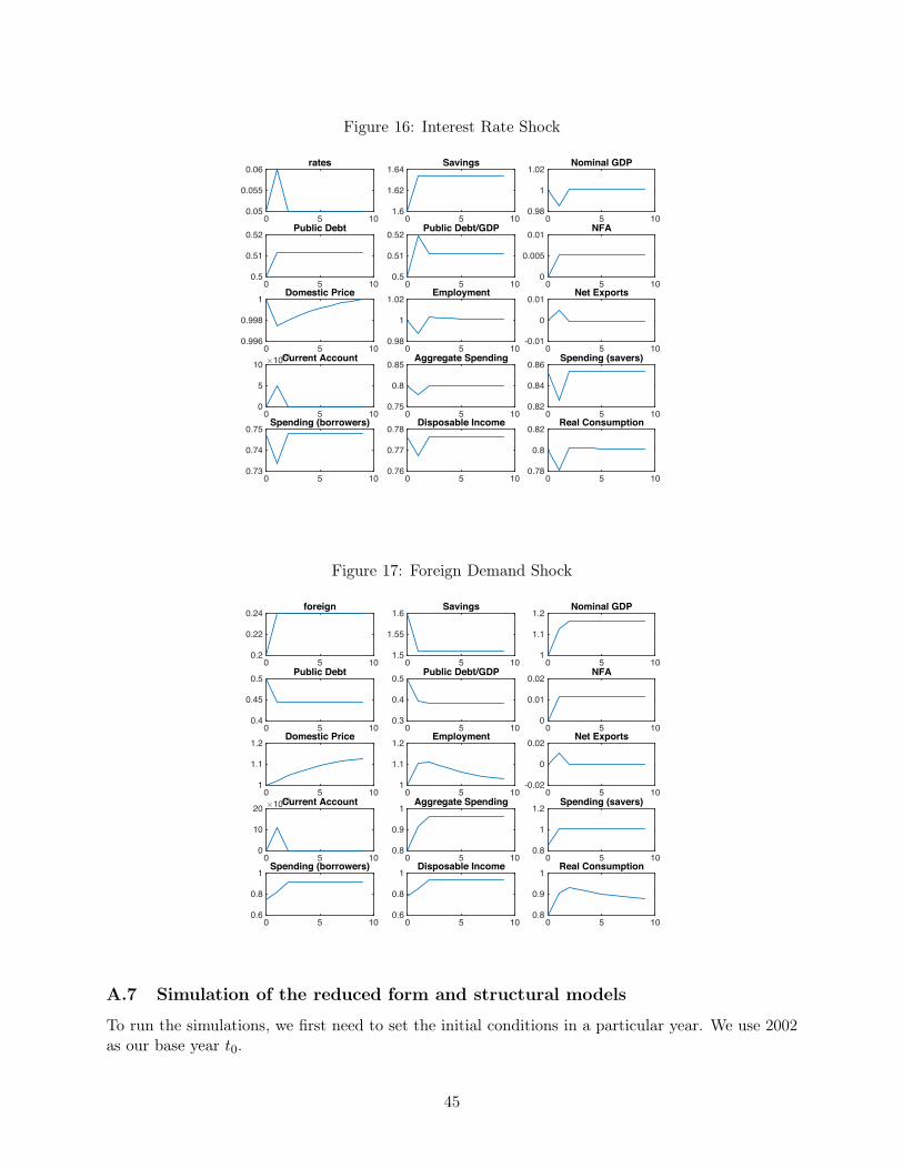
Figure 16: Interest Rate Shock

0 5 100.05

0.055

0.06rates

0 5 101.6

1.62

1.64Savings

0 5 100.98

1

1.02Nominal GDP

0 5 100.5

0.51

0.52Public Debt

0 5 100.5

0.51

0.52Public Debt/GDP

0 5 100

0.005

0.01NFA

0 5 100.996

0.998

1Domestic Price

0 5 100.98

1

1.02Employment

0 5 10-0.01

0

0.01Net Exports

0 5 10

×10-3

0

5

10Current Account

0 5 100.75

0.8

0.85Aggregate Spending

0 5 100.82

0.84

0.86Spending (savers)

0 5 100.73

0.74

0.75Spending (borrowers)

0 5 100.76

0.77

0.78Disposable Income

0 5 100.78

0.8

0.82Real Consumption

Figure 17: Foreign Demand Shock

0 5 100.2

0.22

0.24foreign

0 5 101.5

1.55

1.6Savings

0 5 101

1.1

1.2Nominal GDP

0 5 100.4

0.45

0.5Public Debt

0 5 100.3

0.4

0.5Public Debt/GDP

0 5 100

0.01

0.02NFA

0 5 101

1.1

1.2Domestic Price

0 5 101

1.1

1.2Employment

0 5 10-0.02

0

0.02Net Exports

0 5 10

×10-3

0

10

20Current Account

0 5 100.8

0.9

1Aggregate Spending

0 5 100.8

1

1.2Spending (savers)

0 5 100.6

0.8

1Spending (borrowers)

0 5 100.6

0.8

1Disposable Income

0 5 100.8

0.9

1Real Consumption

A.7 Simulation of the reduced form and structural models

To run the simulations, we first need to set the initial conditions in a particular year. We use 2002as our base year t0.

45

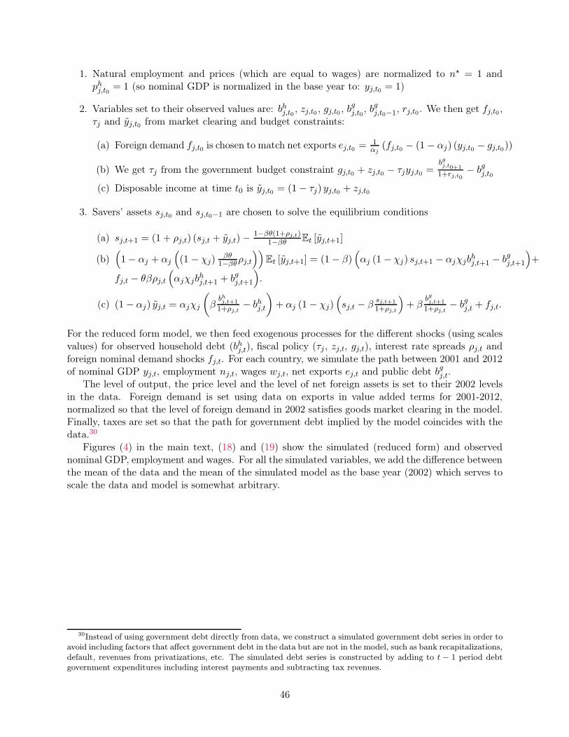
1. Natural employment and prices (which are equal to wages) are normalized to n⋆ = 1 andphj,t0 = 1 (so nominal GDP is normalized in the base year to: yj,t0 = 1)

2. Variables set to their observed values are: bhj,t0 , zj,t0 , gj,t0 , bgj,t0

, bgj,t0−1, rj,t0 . We then get fj,t0 ,τj and yj,t0 from market clearing and budget constraints:

(a) Foreign demand fj,t0 is chosen to match net exports ej,t0 = 1αj

(fj,t0 − (1− αj) (yj,t0 − gj,t0))

(b) We get τj from the government budget constraint gj,t0 + zj,t0 − τjyj,t0 =bgj,t0+11+rj,t0

− bgj,t0

(c) Disposable income at time t0 is yj,t0 = (1− τj) yj,t0 + zj,t0

3. Savers’ assets sj,t0 and sj,t0−1 are chosen to solve the equilibrium conditions

(a) sj,t+1 = (1 + ρj,t) (sj,t + yj,t)−1−βθ(1+ρj,t)

1−βθ Et [yj,t+1]

(b))

1− αj + αj

)

(1− χj)βθ

1−βθρj,t**

Et [yj,t+1] = (1− β))

αj (1− χj) sj,t+1 − αjχjbhj,t+1 − bgj,t+1

*

+

fj,t − θβρj,t)

αjχjbhj,t+1 + bgj,t+1

*

.

(c) (1− αj) yj,t = αjχj

%

βbhj,t+1

1+ρj,t− bhj,t

&

+ αj (1− χj))

sj,t − β sj,t+1

1+ρj,t

*

+ βbgj,t+1

1+ρj,t− bgj,t + fj,t.

For the reduced form model, we then feed exogenous processes for the different shocks (using scalesvalues) for observed household debt (bhj,t), fiscal policy (τj , zj,t, gj,t), interest rate spreads ρj,t andforeign nominal demand shocks fj,t. For each country, we simulate the path between 2001 and 2012of nominal GDP yj,t, employment nj,t, wages wj,t, net exports ej,t and public debt bgj,t.

The level of output, the price level and the level of net foreign assets is set to their 2002 levelsin the data. Foreign demand is set using data on exports in value added terms for 2001-2012,normalized so that the level of foreign demand in 2002 satisfies goods market clearing in the model.Finally, taxes are set so that the path for government debt implied by the model coincides with thedata.30

Figures (4) in the main text, (18) and (19) show the simulated (reduced form) and observednominal GDP, employment and wages. For all the simulated variables, we add the difference betweenthe mean of the data and the mean of the simulated model as the base year (2002) which serves toscale the data and model is somewhat arbitrary.

30Instead of using government debt directly from data, we construct a simulated government debt series in order toavoid including factors that affect government debt in the data but are not in the model, such as bank recapitalizations,default, revenues from privatizations, etc. The simulated debt series is constructed by adding to t − 1 period debtgovernment expenditures including interest payments and subtracting tax revenues.

46

Figure 18: Reduced Form Model, Employment

2001 2004 2008 20120.8

1

AUT

2001 2004 2008 20120.8

1

BEL

2001 2004 2008 20120.8

1

DEU

2001 2004 2008 20120.8

1

ESP

2001 2004 2008 20120.8

1

FIN

2001 2004 2008 20120.8

1

FRA

2001 2004 2008 20120.8

1

GRE

2001 2004 2008 20120.8

1

IRL

2001 2004 2008 20120.8

1

ITA

2001 2004 2008 20120.8

1

NLD

2001 2004 2008 20120.8

1

PRT

year

data

reduced form model

Figure 19: Reduced Form Model, Wages

2001 2004 2008 20120.95

11.05

1.11.15

AUT

2001 2004 2008 20120.95

11.05

1.11.15

BEL

2001 2004 2008 20120.95

11.05

1.11.15

DEU

2001 2004 2008 20120.95

11.05

1.11.15

ESP

2001 2004 2008 20120.95

11.05

1.11.15

FIN

2001 2004 2008 20120.95

11.05

1.11.15

FRA

2001 2004 2008 20120.95

11.05

1.11.15

GRE

2001 2004 2008 20120.95

11.05

1.11.15

IRL

2001 2004 2008 20120.95

11.05

1.11.15

ITA

2001 2004 2008 20120.95

11.05

1.11.15

NLD

2001 2004 2008 20120.95

11.05

1.11.15

PRT

year

data

reduced form model

47

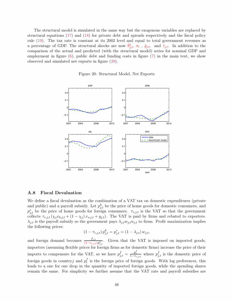
The structural model is simulated in the same way but the exogenous variables are replaced bystructural equations (17) and (18) for private debt and spreads respectively and the fiscal policyrule (19). The tax rate is constant at its 2002 level and equal to total government revenues asa percentage of GDP. The structural shocks are now bhj,t, σt , gj,t. and zj,t. In addition to thecomparison of the actual and predicted (with the structural model) series for nominal GDP andemployment in figure (6), public debt and funding costs in figure (7) in the main text, we showobserved and simulated net exports in figure (20).

Figure 20: Structural Model, Net Exports

2001 2004 2008 2012

−0.1

0

0.1

0.2

ESP

2001 2004 2008 2012

−0.1

0

0.1

0.2

GRE

2001 2004 2008 2012

−0.1

0

0.1

0.2

IRL

2001 2004 2008 2012

−0.1

0

0.1

0.2

PRT

year

databenchmark model

A.8 Fiscal Devaluation

We define a fiscal devaluation as the combination of a VAT tax on domestic expenditures (privateand public) and a payroll subsidy. Let phj,t be the price of home goods for domestic consumers, andp∗j,t be the price of home goods for foreign consumers. τv,j,t is the VAT so that the governmentcollects τv,j,t (χjxb,j,t + (1− χj) xs,j,t + gj,t). The VAT is paid by firms and rebated to exporters.λj,t is the payroll subsidy so the government pays λj,twj,tnj,t to firms. Profit maximization impliesthe following prices:

(1− τv,j,t) phj,t = p∗j,t = (1− λj,t)wj,t,

and foreign demand becomes fj,t(1−τv,j,t)phj,t

. Given that the VAT is imposed on imported goods,

importers (assuming flexible prices for foreign firms as for domestic firms) increase the price of their

imports to compensate for the VAT, so we have pfj,t =pft

1−τv,j,twhere pfj,t is the domestic price of

foreign goods in countryj and pft is the foreign price of foreign goods. With log preferences, thisleads to a one for one drop in the quantity of imported foreign goods, while the spending sharesremain the same. For simplicity we further assume that the VAT rate and payroll subsidies are

48

equal, τv,j,t = λj,t so that phj,t = wj,t, yj,t = wj,tnj,t = pj,tnj,t and domestic prices to domesticconsumers are unchanged. We also assume Et [τv,j,t+1] = τv,j,t. The government budget constraint,is then:

βbgj,t+1

1 + ρj,t+ (τj,t − τv,j,t)wj,tnj,t + τv,j,t(χjxb,j,t + (1− χj) xs,j,t + gj,t) = gj,t + zj,t + Γj,t + bgj,t,

where Γj,t is a lump sum transfer to households. We set this transfer so that the fiscal devaluationis neutral for the government budget constraint in the sense that the budget constraint remains:

βbgj,t+1

1 + ρj,t+ τj,tyj,t = gj,t + zj,t + bgj,t,

so the lump sum transfer is:

Γj,t = τv,j,t(χjxb,j,t + (1− χj) xs,j,t + gj,t)− τv,j,twj,tnj,t.

Market clearing becomes:

nj,t = αjχjxb,j,t + (1− χj)xs,j,t

phj,t+

fj,t(1− τv,j,t)phj,t

+gj,tphj,t

,

and budget constraints are

xb,j,t = βbhj,t+1

1 + ρj,t+ yj,t − bhj,t ; xs,j,t = sj,t + yj,t − β

sj,t+1

1 + ρj,t

where net income is now defined as :

yj,t = (1− τj) yj,t + zj,t + Γj,t

Substitute the government budget constraint and for consumptions from the budget constraintsto get market clearing:

(1− αj) yj,t =)

αj +τv,j,t

1−τv,j,t

*

#

χj

%

βbhj,t+1

1+ρj,t− bhj,t

&

+ (1− χj))

sj,t − β sj,t+1

1+ρj,t

*

$

+ 11−τv,j,t

%

fj,t + βbgj,t+1

1+ρj,t− bgj,t

&

Assuming permanent shocks on foreign demand, Et

,

bgj,t+2

-

= bgj,t+1, small shocks on spreads

and Et [τv,j,t+1] = τv,j,t, expected market clearing at t+ 1 is:

%

1− αj +

%

αj +τv,j,t

1− τv,j,t

&

(1− χj)βθρj,t1− βθ

&

Et [yj,t+1] =

(1− β)

#%

αj +τv,j,t

1− τv,j,t

&

)

(1− χj) sj,t+1 − χjbhj,t+1

*

−%

1

1− τv,j,t

&

bgj,t+1

$

−βθρj,t

0

%

αj +τv,j,t

1− τv,j,t

&

χjbhj,t+1 +

bgj,t+1

1− τv,j,t

1

+fj,t

1− τv,j,t

The fiscal neutrality condition is Γj,t = τv,j,t,

1−αj

αj(yj,t − gj,t) +

1αj

fj,t1−τv,j,t

-

.

49

B For Online Publication: Data Appendix

B.1 Eurozone

Most economic data for Eurozone countries (employment, population, GDP, consumption, gov-ernment debt, expenditures, EU transfers...) comes from Eurostat. We use data for 11 eurozonecountries from 2000 to 2012. Austria, Belgium, Germany, Spain, Finland, France, Greece, Ire-land, Italy, Netherlands and Portugal. We excluded Luxembourg for which household debt data isavailable only starting in 2005 and other countries that joined in 2007 and later.

The data on household debt comes from the BIS which itself compiled the data from nationalcentral banks. This is debt of household and non-profit institutions serving households. Creditcovers all loans and debt securities and comes from both domestic and foreign lenders. The seriescapture the outstanding amount of credit at the end of the reference quarter.

We call government expenditures total government expenditures net of transfers, interest pay-ments and bank recapitalization. The data on spending on bank recapitalization comes fromEurostat. It includes interest payable, capital injections recorded as deficit-increasing (capital trans-fer) and calls on guarantees and is net of revenues generated by bank recapitalization (guaranteefees, interest and dividends). Transfers is the addition of direct social benefits and of social transfersin kind.

Wages and prices, equal in the model, are proxied by the average of unit labor costs and con-sumer prices. Both come from Eurostat and the former are defined as the ratio of labor costs tolabor productivity. For exports we measure the domestic value added that is associated with finalconsumption in the rest of the world, which corresponds to value added based exports. We usethe data from the OECD-WTO Trade in Value-Added (TiVA) initiative to measure domestic valueadded embodied in gross exports. Data is available only in 2000, 2005, 2008 and 2009. For missingyears, we use the ratio of gross exports (from Eurostat) to value added gross exports of the nearestyear and multiply this ratio by the gross exports of the missing year to obtain an approximation ofvalue added exports of the missing years.

We use annual averages of 10 year government bond rates as long term rates. The source isOECD. For the loans rates for SMEs and deposit rates, we use ECB data. SME loans are up to onemillion euros. Data is missing for Belgium (2003-2005), Greece, Ireland, Italy, Portugal (2000-2002)and Portugal (2007-2010). The deposit rates have maturity of up to one year. Irish data is missing.For the other countries, it starts in 2003. For 5 year CDS we use IMF data which starts only in2008.

The source for the TFP in figure (21) is the Conference Board.

B.2 United States

Data for the United States comes from the BEA, the Flow of Funds (FoF), and from the FRBNYConsumer Credit Panel. BEA and FoF data are standard and widely used so we do not discussthem.

The FRBNY Consumer Credit Panel is described in Lee and van der Klaauw (2012). It is anew longitudinal database with detailed information on consumer debt and credit. This panel is arandom sample from consumer credit reports. It is available from 1999 onwards. Credit reportingagencies compile and maintain credit histories for all U.S. residents who have applied for or takenout a loan. Credit bureaus continuously collect information on individual consumers’ debt andcredit from lenders and creditors. Most individuals begin building a credit history when they firstobtain and use a credit or retail card or take out a student loan, usually when they are at least 18years of age. New immigrants with little or no credit history from their home country are often older

50

Figure 21: Changes in Trend TFP Do Not Explain the Eurozone Crisis

AUT

BEL

DEU

ESP

FINFRA

GRE

IRL

ITANLD

PRT

−.2

−.15

−.1

−.05

0.0

5Ch

ange

in E

mpl

oym

ent R

ate

−.04 −.03 −.02 −.01 0 .01Change in trend TFP

Notes: Horizontal Axis is average TFP growth during 2008-2012 minus average TFP growth during 2000-2007(source: Conference Board). Vertical Axis is change in employment rate between 2008 and 2012.

when a credit file is first created for them. The sample design implies that the target populationconsists of all US residents with a credit history. In addition to most individuals younger than 18,who had little need or opportunity for credit activity, the target population excludes individualswho have never applied for or qualified for a loan.

The data at the State level is available in three data sets on the FRBNY web site:

• State level data for all States from 1999 to 2012, annual data for Q4 only.

• Selected states from 1999 to 2003, quarterly data.

• Selected states from 2003 to 2014, quarterly data.

Lee and van der Klaauw (2012) argue that household debt estimates based on the FRBNY Con-sumer Credit Panel are similar to estimates reported in the Board of Governors’ Flow of FundsAccounts. There are differences, however. First, the household debt measures in the Flow of Fundsare not based on direct data but instead are derived as residual amounts. Total mortgage debtand non-mortgage debt in the second quarter of 2010 were respectively $9.4 and $2.3 trillion, thecomparable amounts in the FoF for the same quarter were $10.2 and $2.4 trillion, respectively.

Second, the FoF measure of household mortgage debt includes some mortgage debt held bynonprofit organizations (churches, universities, etc.). On the other hand, FRBNY estimates excludesome debt held by individuals without social security numbers. There may also be differences inthe speed at which changes in various types of debt are recorded, where new mortgage accountsusually appear on credit reports with some delay, making some direct comparisons difficult. Thecomparison is shown in figure (22).

Local Fiscal Policy One potential issue is whether fiscal policy was not also active in the US.Perhaps private debt bubbles were associated with large fiscal revenues and large spending. Thisprobably happened to some extent, but compared to the Eurozone, these effects are small (of coursewe are only talking about cross-sectional variation in government spending). Figure (23) shows thisfor two states and two countries. A regression for all the states and all the countries shows that thelink between private debt and government spending was at least four times smaller in the US thanin Europe.

51

Figure 22: Comparison of Household Debt Measures

Figure 23: Government Spending

.2.2

5.3

.35

.4.4

5

2000 2004 2008 2012year

Spain Ireland Florida Arizona

Government Spending

We therefore argue that the US provides a benchmark for private deleveraging without suddenstops, and with relatively neutral (cross-sectional) fiscal policy.

B.3 Scaled data

The scaled data for household and public debt, government expenditures and transfers, 10 yeargovernment bonds, foreign demand, and spreads and our scaled measure of ρj,t are shown in figures(24), (25), (26) and (27) respectively.

52

Figure 24: Household and Public Debt

0.5

11.

52

0.5

11.

52

0.5

11.

52

2000 2004 2008 2012

2000 2004 2008 2012 2000 2004 2008 2012 2000 2004 2008 2012

AUT BEL DEU ESP

FIN FRA GRE IRL

ITA NLD PRT

Scaled household debt Scaled public debt

year

Graphs by country

Figure 25: Government Expenditures and Transfers

.1.2

.3.4

.1.2

.3.4

.1.2

.3.4

2000 2004 2008 2012

2000 2004 2008 2012 2000 2004 2008 2012 2000 2004 2008 2012

AUT BEL DEU ESP

FIN FRA GRE IRL

ITA NLD PRT

scaled govt exp scaled transfers

year

Graphs by country

53

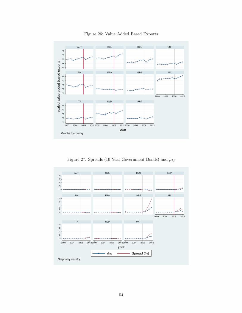
Figure 26: Value Added Based Exports

.1.2

.3.4

.5.1

.2.3

.4.5

.1.2

.3.4

.5

2000 2004 2008 2012

2000 2004 2008 2012 2000 2004 2008 2012 2000 2004 2008 2012

AUT BEL DEU ESP

FIN FRA GRE IRL

ITA NLD PRT

scal

ed v

alue

add

ed b

ased

exp

orts

yearGraphs by country

Figure 27: Spreads (10 Year Government Bonds) and ρj,t

0.0

5.1

.15

.20

.05

.1.1

5.2

0.0

5.1

.15

.2

2000 2004 2008 2012

2000 2004 2008 2012 2000 2004 2008 2012 2000 2004 2008 2012

AUT BEL DEU ESP

FIN FRA GRE IRL

ITA NLD PRT

rho Spread (%)

year

Graphs by country

54