ORI GIN AL PA PER

Instability, investment, disasters, and demography:natural disasters and fertility in Italy (1820–1962)and Japan (1671–1965)

C.-Y. Cynthia Lin

Published online: 19 February 2010

� The Author(s) 2010. This article is published with open access at Springerlink.com

Abstract This article examines whether natural disasters affect fertility—a topic

little explored but of policy importance given relevance to policies regarding

disaster insurance, foreign aid, and the environment. The identification strategy

uses historic regional data to exploit natural variation within each of two coun-

tries: one European country—Italy (1820–1962), and one Asian country—Japan

(1671–1965). The choice of study settings allows consideration of Jones’ (The

European miracle, Cambridge University Press, Cambridge, 1981) theory that

preindustrial differences in income and population between Asia and Europe

resulted from the fertility response to different environmental risk profiles.

According to the results, short-run instability, particularly that arising from the

natural environment, appears to be associated with a decrease in fertility—thereby

suggesting that environmental shocks and economic volatility are associated with

a decrease in investment in the population size of future generations. The results

also show that, contrary to Jones’ (The European miracle, Cambridge University

Press, Cambridge, 1981) theory, differences in fertility between Italy and Japan

cannot be explained away by disaster proneness alone. Research on the effects of

natural disasters may enable social scientists and environmentalists alike to better

predict the potential effects of the increase in natural disasters that may result

from global climate change.

Keywords Natural disasters � Fertility � Environmental shock � Instability

C.-Y. C. Lin (&)

Agricultural and Resource Economics, University of California at Davis,

One Shields Avenue, Davis, CA 95616, USA

e-mail: cclin@primal.ucdavis.edu

123

Popul Environ (2010) 31:255–281

DOI 10.1007/s11111-010-0103-3

Introduction

Dynamic demographic–economic relationships have been of interest to social

scientists ever since Malthus proposed an economic theory of population growth in

the late eighteenth century (see e.g., NBER 1960; Schofield and Wrigley 1985;

Lindahl-Kiessling and Landberg 1994; Galor 2004). However, while it may describe

long-run relationships between population and income in preindustrial Western

societies, the classical Malthusian theory fares less well in more general contexts.

One possible reason is that, in focusing primarily on the extent to which wages and

vital rates exert influence on each other in steady state over the long run of several

generations, the classical theory has overlooked the possible effects of environ-

mental shocks and other forms of short-run instability on the demographic–

economic system that occur within a single generation.

Individuals behave differently under conditions of instability, risk, and uncer-

tainty than they do under conditions of perfect certitude. For example, ample

empirical evidence suggests that household-level income volatility leads to lower

investment in both physical and human capital at the micro level, and that country-

level economic volatility leads to lower government spending and lower mean

growth at the macro level (Blattman et al. 2007, and references therein). In a similar

fashion, sources of instability are likely to affect fertility decisions as well.

According to Cain (1983): ‘‘If people are motivated by a principle of safety-first,

[their fertility behavior] may be influenced less by average mortality experience

than by variance in that experience, and particularly the tail of the distribution that

contains the worst records’’ (p. 698). Just as individuals in unstable economic

environments may be less willing to invest in capital, individuals in volatile natural

environments may be less willing to invest in bearing children.1

The purpose of this article is to expand upon the existing literature on population

and the economy by examining whether natural disasters affect fertility. The

identification strategy uses regional data to exploit the natural variation within each

of two countries: one European country—Italy, and one Asian country—Japan. The

time periods under consideration are 1820–1962 for Italy and 1671–1965 for Japan.

An analysis of the effects of environmental shocks on fertility is important for

two reasons. First, because there are considerable differences in the stability of the

natural environment across the world, studies of the effects of environmental

shocks on demographic–economic relationships may enable economists to better

understand the sources of cross-country differences in population growth and

income.

There is an extensive literature that theoretically and conceptually discusses the

consequences of population growth on a country’s economy (see e.g., Lee and

Edwards 2001; Coale and Hoover 1969; Spengler 1969; Stavig 1979, and references

therein). In his empirical study of 94 countries over the period 1955–1971, Stavig

(1979) finds that rapid population increase had a negative impact on changes in

many crucial economic indicators—including change in per capita gross capital

1 In this article, the phrase ‘‘investing in children’’ is used to capture the bearing of new children rather

than investments in the health and education of existing children.

256 Popul Environ (2010) 31:255–281

123

formation, government consumption, manufacturing, and exports—many of which

are highly correlated to change in per capita GNP.

If population size affects the living standard, then an understanding of all the

factors influencing population growth, including environmental ones, is essential for

understanding global income inequality and past, current, and future economic

development. For instance, Jones (1981) makes the bold claim that differences in

Asian and European population growth and income prior to the Industrial

Revolution were due to the fertility response to different risk profiles; Asia’s

natural disaster-prone environment was to blame for its lower income.

A second reason why research on environmental shocks is important is that it has

implications for policies regarding disaster insurance, foreign aid, and the

environment. For example, if natural disasters cause a decrease in fertility because

they make families reluctant to invest in having children, then risk-sharing policies

such as disaster insurance can help mitigate these effects. Similarly, if economic

volatility is associated with a decline in fertility, then foreign aid policies that

minimize the volatility can attenuate the impact on fertility.

In addition to the relationship between environmental shocks and fertility, this

article also examines the relationship between economic volatility and fertility.

Economic volatility is included as well because it is another form of short-run

instability that may affect fertility, and because economic volatility has been found

in other studies to lower investment in physical and human capital (Blattman et al.

2007, and references therein). This article examines whether economic volatility,

like environmental instability, may be associated with changes in fertility.

Italy and Japan were chosen for the empirical analysis based on the following

factors: the availability of region-level data, the prevalence of natural disasters,

and the need for a country each from Europe and Asia. The choice of two natural

disaster-prone countries, one from Europe and one from Asia, enables one to

build upon Jones’ (1981) theory that differences in fertility behavior in Asia and

Europe were a result of differences in the prevalence of natural disasters—not

differences in culture, society, history, or politics—and, therefore, that any other

society subjected to the volatility of the Asian environment would have responded

in a similar manner. This article is a first cut at comparing causes of historical

fertility in Asia and Europe; a more thorough analysis will be the subject of

future study.

According to the results, natural disasters have a significant association with

fertility in both countries. In Italy, earthquakes had a robust negative association

with fertility, particularly marital fertility. In Japan, tsunamis had a robust negative

association with fertility while earthquakes had a significant positive association

with fertility in some specifications. Short-run economic volatility has a significant

negative association with fertility in Italy, but no association in Japan.

The remainder of this article is as follows. Section ‘‘Previous literature’’ surveys

the relevant literature. Section ‘‘Determinants of fertility’’ describes the mecha-

nisms through which income, mortality, and instability may affect fertility. The data

are described in Section ‘‘Data’’, and the estimation methodology is described in

Section ‘‘Econometric methodology’’. Results are presented in Section ‘‘Results’’.

Section ‘‘Concluding remarks’’ concludes.

Popul Environ (2010) 31:255–281 257

123

Previous literature

Environment, demography, and economic growth

This article relates to several existing branches of literature. First, it draws upon the

literature on the effects of the environment on economic development (see e.g.,

Diamond 1997; Gallup et al. 1999; Sachs 2001; Boserup 1996; Pebley 1998), and

the literature on the link between economic growth and population growth (Bloom

and Sachs 1998; Bloom and Williamson 1998; Bloom et al. 2003).

This article relates most closely to the study of Portner (2006), who uses data on

hurricanes in Guatemala over the last 120 years combined with a recent household

survey to analyze how decisions on education and fertility respond to hurricane risk

and shocks. By measuring risks and shocks separately, Portner is able to separate

out the impact of shocks on fertility in the short-run from the impact of risk on

fertility in the long-run. Portner uses the average percent chance of being hit by a

hurricane in a year, as averaged over all the years in his data, as his measure of risk.

Risk is, therefore, a time-invariant variable. By using county fixed effects that

absorb the effect of all county-level time invariant variables, including risk, this

article similarly controls for risk to identify the short-run effect of an environmental

shock.

This article also relates to the study of Kalipeni (1996), whose analysis of the

demographic response to environmental pressure in Malawi finds that areas that are

experiencing intense environmental pressure are also beginning to go through a

fertility transition. In particular, Kalipeni finds evidence of declining fertility rates

in response to environmental pressure particularly in areas with high population

densities. This article similarly examines the association between the environment

and fertility.

Previous studies have shown that instability in the environment in the form of

famines and wars have a negative effect on fertility. In his analysis of South Asian

famines, Dyson (1991) finds a reduction in conceptions prior to a famine even

without a major rise in the death rate, perhaps due to conscious planning during the

periods of mounting adversity preceding a famine. Boyle and Grada (1986) find that

at the onset of the Great Irish Famine of 1845–1849, the fertility rate dropped to

75% of its pre-Famine level and remained at this level for the duration of the

famine. In their study of Angola et al. (2002) find evidence of a wartime drop in

fertility. In their study of Cambodia et al. (2007) find a one-third decline in fertility

during the Khmer Rouge regime, under which 25% of the Cambodian population

died.

Asia versus Europe

The choice to examine both an Asian country and a European country relates to

Jones’ (1981) theory that preindustrial differences in income and population

between Asia and Europe resulted from the fertility response to different

environmental risk profiles.

258 Popul Environ (2010) 31:255–281

123

According to Jones’ theory, because Asians were faced with a more natural

disaster-prone environment, they accumulated a population surplus as a form of

demographic insurance against catastrophe; they, therefore, had a higher fertility

rate, a higher marriage rate, and a lower age at marriage in steady state than their

European counterparts did. This strategy of family size maximization resulted in

lower consumption levels, lower savings rate, less investment in human capital, and

larger disparities in income in Asia than in Europe. Thus, according to Jones,

preindustrial differences in environmental risk had dire consequences on social and

economic inequality both within and between the two regions. Natural disasters

were to blame for Asia’s relative poverty. Moreover, Jones claims, demographic

choices were a result of the risk profile of the environment; if the risk profile were to

change, then the steady-state choices would change as well.

This article expands upon Jones’ study in two main ways. Jones uses measures of

the incidence and effects of a natural disaster that are potentially endogenous to

fertility. For example, one measure Jones uses is the death toll from a disaster,

which is endogenous because it depends in part on the population density, which is

in turn affected by fertility. In contrast, this article instead uses measures that are

exogenous: the number and geophysical magnitude of disasters, neither of which are

affected by fertility.

The second innovation in this article is that is focuses on the short-run behavioral

effects of a disaster rather than its long-run steady-state implications. While the

long-run steady state takes place over centuries and multiple generations, short-run

behavioral effects take place over decades, within a single generation. Jones’ theory

describes the steady-state relationships among population growth, economic

development, and environmental instability. While greater environmental instability

may lead to greater population growth in the long-run steady state, it is likely that

the effect might be the opposite during short-run transitions. In the immediate

aftermath of a disaster, one might expect risk-averse individuals to react by

decreasing, rather than increasing, long-term investments in assets such as children.

The latter short-run behavioral response is the focus of this article.

Volatility and investment

This article also innovates upon the burgeoning literature linking economic

volatility to lower investment. At the microeconomic level, empirical evidence

suggests that households respond to income volatility by diversifying and skewing

their income-generating activities toward low-risk alternatives with lower returns,

thereby decreasing their investment in physical and human capital (Blattman et al.

2007, and references therein). For example, Rosenzweig and Wolpin (1993) find

that risk-averse farmers faced with borrowing constraints and low and uncertain

incomes underinvest in assets needed for agricultural production and consumption

smoothing, thus leading to output losses, lower incomes, and greater income

volatility. Similarly, income volatility causes parents to underinvest in the health

and education of their children (Frankenberg et al. 1999; Thomas et al. 2004).

Empirical evidence suggests that economic instability decreases investment at

the macroeconomic level as well. For example, in their examination of 92

Popul Environ (2010) 31:255–281 259

123

developed and developing economies between 1962 and 1985, Ramey and Ramey

(1995) find that countries with high macroeconomic volatility have lower

government spending and lower mean growth. Countries that face borrowing

constraints and terms of trade shocks may have difficulty smoothing public

investment and expenditure (Blattman et al. 2007).

In some ways, giving birth to a child is a form of investment just as investing in

capital is. As noted by Becker (1960), children are a durable consumption and

production good. The motives for having children may include both the direct

satisfaction children are expected to provide their parents and the indirect

satisfaction they may render by working in the household or family business or

by remitting money income to their parents (Willis 1973). In traditional societies,

children are beneficial to parents from an early age as a source of labor; they

represent an investment for support in old age, an insurance against risk in a

hazardous environment, and enhance the physical security and political influence of

the family unit (Cleland and Wilson 1987). Childbirth requires huge up-front costs

in terms of time and money, and the potential insurance benefits of having children

accrue in the future. Economic uncertainty can, therefore, lead to lower levels of

fertility (Kohler et al. 2002; Perelli-Harris 2005). This article expands on the

literature connecting income volatility with lower capital investment and depressed

long-run economic performance by examining whether natural disasters and

economic volatility affects investment in the future population size.

Determinants of fertility

What factors determine fertility? The classical Malthusian theory posits that fertility

is affected by income and mortality; the hypothesis of this article is that short-run

shocks should have an effect as well. This section describes the mechanisms through

which each of these factors may affect fertility.

There are several possible theories for how fertility may respond to income.

Malthusian theory predicts that wages should have a positive effect on fertility

through its effect on increasing the marriage rate (Lee and Wang 1999), perhaps

because in Europe, couples could not marry before they acquired an economic

means of support (Lee 1973). Another possible reason for a positive relationship

between wages and fertility is that higher incomes lead to better nutrition, which in

turn enhances fecundity (Lee 1985). Moreover, because children are a consumer

durable, an increase in income should increase both the quality and quantity of

children (Becker 1960).

On the other hand, it is also possible for higher wages to have a negative effect on

fertility. One reason why fertility may decrease with income is that higher wages

diminish the need for children as a form of insurance. For instance, higher income

levels may be associated with the development of other forms of insurance (Cleland

and Wilson 1987). A second reason is that higher income levels may be associated

with a stronger social custom against marriage or a stronger social custom favoring

quality of children rather than quantity. Third, when one’s earnings in the labor

market are high, then the opportunity cost of marriage and of raising children are

260 Popul Environ (2010) 31:255–281

123

high as well (Mason 1997). Thus, because theory suggests that wages can have

either a positive or negative effect on fertility, it is possible that wages have no net

effect.

In addition to the wage, a second determinant of fertility that is included in the

Malthusian model is the crude death rate. The classical economic theory of

population growth predicts that fertility should increase with mortality. For

example, if couples desire to have a certain number of surviving children, then

higher rates of infant and child mortality would induce higher levels of marital

fertility, for parents would endeavor to replace the children they have lost. Likewise,

in some preindustrial populations, age at death of one’s father would affect the

timing of inheritance and, therefore, of one’s marriage (Lee 1973), so that a higher

death rate would lead to earlier marriage and, therefore, a higher birth rate as well.

On the other hand, as with other forms of risk, mortality risk may affect

individual behavior and, in particular, reduce long-term investing. To the extent that

the crude death rate is a measure of mortality risk, therefore, it is possible that

fertility decreases with mortality. For instance, if child death rates are high, then

children become a more risky investment, and parents may choose to invest less in

having them. Likewise, if adult death rates are high, then parents may be more

cautious about having a child if they do not believe they will live long enough to

care for the child, or long enough to reap any potential old age insurance benefits

from investing in children.

While the classical economic theory has focused primarily on income and

mortality, this article focuses instead on an additional determinant of fertility:

environmental shocks, as measured by the number and magnitude of natural

disasters. Income and mortality are used as controls. According to Jones (1981),

who hypothesized that families living in a more natural disaster-prone environment

would accumulate a population surplus as a form of demographic insurance against

catastrophe, one would expect natural disasters to have a positive effect on fertility.

However, it is also possible that short-run environmental shocks may decrease

fertility, perhaps because the shock makes individuals less willing to make the long-

term investments required to raise a family. Another reason individuals might have

lower fertility in the short run after an environmental shock is that the disaster

causes a disruption in family life and social organization, for example by causing

the death and/or break-up of families, by destroying houses, or by causing

individuals to lose their jobs. This article investigates the effects of short-run

environmental shocks, and, therefore, hypothesizes that environmental shocks are

associated with a decrease in fertility.

In addition to natural disasters, a second form of short-run instability considered in

this article is economic volatility, as measured by the variance of the detrended wage.

Economic theory predicts that greater economic volatility will lower investment in

human and physical capital (Blattman et al. 2007). In this article, it is hypothesized

that, like natural disasters, greater economic volatility will also lower the investment

in the future population size, and is, therefore, associated with lower fertility.

Social factors influence fertility as well. Societal norms about reproduction affect

fertility (Munshi and Myaux 2006; Thomson and Goldman 1987). Fertility

decisions often occur in specified social contexts. For example, a woman’s social

Popul Environ (2010) 31:255–281 261

123

network and social world may affect her fertility behavior (Madhavan et al. 2003).

Social influences would affect the short-run and long-run responses to shocks. These

social factors are addressed in several ways. First, analyzing Italy and Japan

separately allows for country-level social differences between the two countries.

Second, a region-level fixed effects model allows for region-level social factors.

Third, a spatial model allows for social spillovers between neighboring regions, and,

therefore, for social networks that may possibly spill over from one region to the

next.2

Data

Demographic, economic, and disaster data for Italy (1820–1962) and Japan (1671–

1965) are used. Data from many countries were initially gathered, but Italy and Japan

were chosen for the final analysis based on the following factors: the availability of

region-level data, the prevalence of natural disasters, and the need for a country each

from Europe and Asia.3 The choice of two natural disaster-prone countries, one from

Europe and one from Asia, enables one to build upon Jones’ (1981) theory that

differences in fertility behavior in Asia and Europe were a result of differences in the

prevalence of natural disasters—not differences in culture, society, history, or

politics—and, therefore, that any other society subjected to the volatility of the Asian

environment would have responded in a similar manner. The data sources used for

Italy and Japan are detailed in Appendixes 1 and 2, respectively.

Demographic data were compiled from various print sources or extracted from

the Princeton European Fertility Project online demographic data set (Treadway

1980). These variables include the following measures of fertility: crude birth rates,

the index of total fertility (If), the index of marital fertility (Ig), and the index of

non-marital fertility (Ih).4 They also include crude death rates. The print sources for

2 These models also address possible country-level or region-level biological influences as well.3 Other countries and regions for which data were initially gathered include: Austria-Hungary, Belgium,

China, Denmark, England, France, Germany, India, Netherlands, Romania, Scandinavia, Serbia, Sweden,

Southeast Asia, Switzerland, and Taiwan, but these countries were not used because region-level panel

data for crude birth rates and crude death rates were too sparse, and/or natural disasters were too

infrequent.4 If is defined as the ratio of the number of births the women in a given population actually have to the

number they would have had if they were subjected to a maximal well-recorded age-specific fertility

schedule (that of the Hutterites). Ig is defined as the ratio of the number of births the married women in a

given population actually have to the number they would have had if they were subjected to the maximal

age-specific fertility schedule. Ih is the ratio of the number of births the unmarried women in a given

population actually have to the number they would have had if they were subjected to the maximal age-

specific fertility schedule. The index of marital status (Im), which is not used in this article, is the ratio of

the number of births married women would experience if subjected to the maximal age-specific fertility

schedule to the number of births all women would experience if subjected to that same maximal fertility

schedule; it is an index of the extent to which the marital status distribution would contribute to the

attainment of maximal fertility in a population in which all births were to married women.

The fertility indices have the following relationship:

If � Im � Igþ 1��Imð Þ � Ih

(Treadway 1980).

262 Popul Environ (2010) 31:255–281

123

Italy’s demographic data are Livi-Bacci (1977) and del Panta (1979). The print

sources for Japan’s demographic data are Hanley and Yamamura (1977); Morris and

Smith (1985); Smith (1977); Jannetta and Preston (1998).

Annual real wage data were from Jeffrey Williamson: the Italian wage index

(1900 = 100) was taken from Williamson (1995) while the Japanese wage index

(1934–1936 = 100) was provided in digital form. This wage data was used to

calculate, for each year, the variance of the detrended wage over the past 20 years

prior to and including that year in the base case.5 Whenever possible, the variables

for both the level and the variance of the wage were averaged over the same years

over which observations for the demographic dependent variable spanned in any

given regression.6 All averages were centered on the floor of the midpoint of the

years covered in the average.

Daily natural disaster data on the number and magnitudes of earthquakes,

tsunamis, and volcanos were taken from the National Geophysical Data Center web

site (Dunbar et al. 1999; Lockridge 1999; Whiteside 1999). In order to measure the

severity of the earthquake, either the Modified Mercalli Intensity Scale of 1931,

which takes on integer values from 1 (least intense) to 12 (most intense); or the

geophysical magnitude, where each increase in magnitude represents a 10 fold

increase surface wave amplitude,7 is used. The magnitude of a tsunami is defined as

the log of twice the maximum runup height of the wave; this value is incremented

by 2, so that the minimum value is 1 instead of –1.8 For the volcano magnitude, the

volcano explosivity index is incremented by 1, so that it takes on integer values

from 1 (tephra volume = 1E4, column height \0.1 km above crater) to 9 (tephra

volume C1E12, column height[25 km above sea level). For all types of disaster, a

magnitude or intensity of 0 denotes no disaster.

From the raw natural disaster data, variables are constructed for each year in the

data set for (1) the number of each type of disaster over the past 20 years prior to

and including that year, and for (2) the sum of the geophysical magnitudes of all

occurrences of earthquakes, tsunamis, and volcanos over the past 20 years prior to

and including that year. For example, for the 1880 observation, environmental

shocks are aggregated over 1861–1880. When multiple observations existed for any

given disaster, an average of the magnitudes reported was taken.

In the base case, both the measure of environmental shock and the measure of

short-run economic volatility consider events that have occurred over the previous

20 years. This is because individuals who are making choices about marriage,

5 The variance of the wage was then divided by 1000 so that the magnitude of its coefficients in the

various regressions would not be too small.6 Some of the original wage data for preindustrial epochs has already been interpolated over several

years.7 While some records report both the earthquake magnitude and the earthquake intensity, others report

only one. Whether the earthquake magnitude or the earthquake intensity is used in the regressions as the

measure of the severity of the earthquake depends on which variable has more observations for that

country. When an earthquake occurs but either the magnitude or the intensity is not reported, then this

value is coded as missing, not 0 (which denotes no disaster).8 This enables 0 to denote no disaster.

Popul Environ (2010) 31:255–281 263

123

childbearing, and potential tradeoffs with their careers do so in their early twenties,9

and, therefore, have experienced the previous two decades of environmental

disasters and economic instability. As a robustness check, the previous 10 years is

also used to measure short-run instability.10

The demographic, economic, and natural disaster data are used to construct a

panel data set for Italy and a panel data set for Japan.

For the Italian panel, the unit of observation is a region. There are 18 regions in

Italy; following del Panta (1979), these regions can be grouped into five

geographical areas: Northwest, Northeast, Center, South, and Islands. The panel

covers all 18 regions and spans the years 1820–1962. While measures of fertility

were available at the region level, the measures of mortality compiled were at the

level of the geographical area.11 Thus, for each geographical area, the area’s values

for the crude death rates were used for all regions in the area. The same national

Italian wage data, which reflect mainly the wages in Northern Italy, were applied to

all regions. Volcano data were matched to the region in which the volcano was

located. All other natural disaster data were matched to the region based on the

location(s) named in the source, or, when the location name could not be located in

any region, on the latitudes and longitudes given. Disasters that occur in areas larger

than a region are assumed to strike all regions in that area; disasters that occur in

areas smaller than a region are assumed to affect the entire region.

In the panel data set for Italy, the fertility variables generally each span 3 years per

observation. For example, for the fertility indices, there are up to 11 observations of

each fertility index for each region: (1) 1862–1866, (2) 1870–1872, (3) 1880–1882,

(4) 1890–1892, (5) 1900–1902, (6) 1910–1912, (7) 1921–1926, (8) 1930–1932,

(9) 1935–1937, (10) 1950–1952, and (11) 1960–1962. Of the 18 regions, 14 regions

have observations during 1862–1866, and 16 regions have observations during

1870–1912; all the 18 regions have observations from 1921–1962. For the crude birth

rate data, there are several more observations over other 3-year intervals for some of

the regions, so the crude birth rate data extends back to 1820.

Because the fertility data spans mostly 3 years per observation, the natural

disaster variables, which represent the sum of either the number or intensity of

natural disasters over the last 10 or 20 years, are averaged over 3 years. Similarly,

9 For the data gathered for this article, the minimum mean age at marriage for females was 21.8 for Italy

and 22.9 for Japan. For men in Italy, the minimum mean age at marriage is 27.1 (Lin 2004). The data set

compiled does not include data on the mean age at marriage for men in Japan.10 The measure of shocks used by Portner (2006) is the number of hurricanes between the year the

woman enters her fertility period, taken to be 15 years, and her 29th year (thus spanning a 14-year time

period) or the survey year, whatever is first. The reason for the 29-year cutoff is that the majority of

women have most of their children before they turn 30.11 The few figures that were found for regional crude death rates covered only seven regions with only 2–

6 observations each (del Panta 1979, p. 226). Moreover, periods of major crises were excluded from these

data; such an exclusion would bias the results of this study. Another alternative would be to calculate

regional averages from the provincial crude death rates reported in Hoffman (1981). I chose not to do so

for this study because the provincial data covered fewer time intervals than the geographical data did (5

per province as opposed to 9 per geographical area).

264 Popul Environ (2010) 31:255–281

123

the real wage and the variance of the wage (which is the variance in the detrended

wage over the past 10 or 20 years, divided by 1000) are averaged over 3 years as

well. Because the wage data begin in 1871, and because at least 10 prior years of

wage data are needed to form the variance of the wage, the regressions that

include the variance of the wage span the years 1880–1962. Geographical area-

level crude death rates span 4–5 years per observation. All the variables spanning

multiple years are centered on the floor of the midpoint of the years covered in the

average. For example, for each region in Italy, a birth rate that spans the three

years 1880–1882 is coupled with the average of the natural disaster variable for

the three 20-year ranges 1861–1880, 1862–1881, and 1863–1882, and the

observation is centered on the floor of the midpoint of the years covered in the

average, which in this case is the year 1881, the midpoint of 1880–1882. See

Appendix 1.

The Japan panel consists of data from 13 mura (villages), one shi (city) and one

han (domain), and spans the years 1671–1965. For lack of a better term, the level at

which an observation applies—whether it be a village, city or domain—is called a

‘‘place.’’ Observations are available for different years for each place, and each unit

of observation covers from 1 to 41 years depending on the place. For example, for

the domain, Morioka, there are 15 1-year observations: one every 10 years from

1680 to 1790, and also the years 1803, 1828, and 1840. The observations for the

other places cover different years. Each of the places can be matched to one of the

11 regions in Japan. Regressions include either place or region fixed effects.

The same national Japanese wage data were applied to all places; the data

were constructed by Jeffrey Williamson from pre-1930 wage data for Kyoto and

Kamikawarabayashi (near Osaka) and post-1930 wage data for Tokyo. The wage

data span the years 1727–1938. Volcano data were matched to the prefecture in

which the volcano was located. All other natural disaster data were matched to

the prefecture based on the location(s) named in the source, or, when the

location name could not be located in any prefecture, on the latitudes and

longitudes given. Disasters that occur in areas larger than a prefecture are

assumed to strike all prefectures in that area; disasters that occur in areas smaller

than a prefecture are assumed to affect the entire prefecture. All the places are

assumed to be affected by the disasters matched to the prefecture(s) in which

they are located.

For the panel data set for Japan, crude birth rates span 1–41 years per

observation, with an average span of approximately 10 years. Consequently, the

natural disaster variables, which represent the sum of either the number or intensity

of natural disasters over the last 20 years, are averaged over 10 years. Similarly, the

real wage and the variance of the wage (which is the variance in the detrended wage

over the past 10 years, divided by 1000) are averaged over 10 years as well.

Because the wage data span the years 1727–1938, and because at least 10 prior

years of wage data are needed to construct the variance of the wage variable, the

regressions that include the variance of the wage span the years 1737–1935. Crude

death rates span the same number of years as the crude birth rate for each

observation. All variables spanning multiple years are centered on the floor of the

midpoint of the years covered in the average. See Appendix 2.

Popul Environ (2010) 31:255–281 265

123

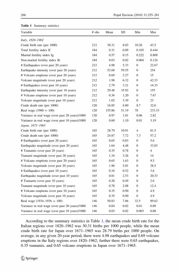
According to the summary statistics in Table 1, the mean crude birth rate for the

Italian regions over 1820–1962 was 30.31 births per 1000 people, while the mean

crude birth rate for Japan over 1671–1965 was 28.79 births per 1000 people. On

average, in any given 20-year period, there were 4.98 earthquakes and 0.69 volcano

eruptions in the Italy regions over 1820–1962; further there were 0.65 earthquakes,

0.35 tsunamis, and 0.65 volcano eruptions in Japan over 1671–1965.

Table 1 Summary statistics

Variable # obs Mean SD Min Max

Italy, 1820–1962

Crude birth rate (per 1000) 212 30.31 8.03 10.26 43.5

Total fertility index If 184 0.31 0.09 0.105 0.444

Marital fertility index Ig 184 0.57 0.15 0.222 0.809

Non-marital fertility index Ih 184 0.03 0.02 0.004 0.124

# Earthquakes (over past 20 years) 212 4.98 5.33 0 22.67

Earthquake intensity (over past 20 years) 212 52.60 59.55 0 254

# Volcano eruptions (over past 20 years) 212 0.69 2.27 0 15

Volcano magnitude (over past 20 years) 212 1.98 6.32 0 42.33

# Earthquakes (over past 10 years) 212 2.79 3.21 0 14.33

Earthquake intensity (over past 10 years) 212 29.48 35.92 0 155

# Volcano eruptions (over past 10 years) 212 0.36 1.20 0 7.67

Volcano magnitude (over past 10 years) 212 1.02 3.39 0 23

Crude death rate (per 1000) 120 16.85 6.80 8.7 32.6

Real wage (1900 = 100) 120 155.86 51.19 78 233.33

Variance in real wage (over past 20 years)/1000 120 0.97 1.01 0.06 2.82

Variance in real wage (over past 10 years)/1000 120 0.60 1.10 0.01 3.19

Japan, 1671–1965

Crude birth rate (per 1000) 165 28.79 10.91 4 81.5

Crude death rate (per 1000) 165 24.87 7.72 7.3 57.2

# Earthquakes (over past 20 years) 165 0.65 0.83 0 5.6

Earthquake magnitude (over past 20 years) 165 1.64 4.48 0 33.83

# Tsunamis (over past 20 years) 165 0.35 0.78 0 4

Tsunami magnitude (over past 20 years) 165 1.34 3.26 0 14

# Volcano eruptions (over past 20 years) 165 0.65 1.63 0 9.5

Volcano magnitude (over past 20 years) 165 1.96 5.01 0 28.5

# Earthquakes (over past 10 years) 165 0.34 0.52 0 3.6

Earthquake magnitude (over past 10 years) 165 0.81 2.53 0 20.33

# Tsunamis (over past 10 years) 165 0.20 0.49 0 2.6

Tsunami magnitude (over past 10 years) 165 0.78 2.08 0 12.4

# Volcano eruptions (over past 10 years) 165 0.35 0.90 0 4.9

Volcano magnitude (over past 10 years) 165 0.35 0.90 0 4.9

Real wage (1934–1936 = 100) 146 50.83 7.86 32.5 89.62

Variance in real wage (over past 20 years)/1000 146 0.04 0.02 0.01 0.09

Variance in real wage (over past 10 years)/1000 146 0.03 0.02 0.003 0.08

266 Popul Environ (2010) 31:255–281

123

Econometric methodology

The identification strategy employed in this article uses regional data to exploit

natural within-country variation for both Italy and Japan. With panel data, region

fixed effects can be used to control for time-invariant, region-specific omitted

variables such as local culture or local attitudes toward risk or mortality, or local

economic factors; and the country-specific time trend (the coefficient on year) can

be used to control for national trends including country-level changes in social

attitudes, cultural values, network behavior, and/or people’s fertility preferences.

The fixed effects also control for the average long-run steady-state environmental

risk faced by a particular region, thus enabling one to identify the effects of a short-

run environmental shock. The fixed effects similarly control for steady-state

differences in the economic volatility of different regions (e.g., their local economic

risk profiles).

The primary innovation of this article is to include measures of short-run

instability in traditional regressions of fertility on income and mortality. The

number and magnitudes of natural disasters are used to measure environmental

shocks and the variance of the detrended wage is used to measure economic

volatility.12 The joint significance of the natural disaster variables as well as the

joint significance of the economic variables are tested.

All regressions are OLS. For the economic variables, it is, therefore, assumed that

neither the real wage nor the variance of the wage is likely to be endogenous to the

contemporaneous birth rate because babies are too young to have an effect on the

labor market.13 For environmental shocks, exogenous measures are used:

the number and geophysical magnitude of natural disasters, neither of which are

affected by fertility.

For the crude death rate, one potential omitted variable that may cause the crude

death rate to be endogenous to fertility is famine, which not only elevates mortality

but also depresses fertility (Lee 1985; Maharatna 1996). Controlling for natural

disasters addresses this problem, at least in part, as natural disasters are often a cause

of famine. Moreover, any endogeneity of mortality to fertility would operate

through the number of births, not the birth rate. Fortunately, there does not appear to

be any major documented famine either in Italy over the period 1820–1962 or in

Japan over the period 1671–1965.14 Thus, it is assumed that, as with the other

regressors, the crude death rate is exogenous as well.

In using historical data, one may worry that the data may be noisy measurements

of the true values. Classical measurement error biases the coefficients toward zero

(Wooldridge 2002), which means that the effects may be underestimated. Thus, the

12 Previous regressions also included the minimum and the maximum of the detrended wage over the

past 10 years. However, because these variables did not turn out to be significant and because they had

little effect on the coefficient estimates of the other variables, but merely served to depress the degrees of

freedom, I excluded them in the analysis presented here.13 It is possible that the birth rate may affect wages through, for example, the wages of pediatricians, of

childcare professionals, or the labor supply of women, but I assume that these effects are not of first-order.14 See e.g., the list of famines in Walford (1970).

Popul Environ (2010) 31:255–281 267

123

results provide lower bounds to the magnitudes of the effects of natural disasters and

economic volatility.

Because local economic data were not available for the time periods and regions

analyzed, the fixed effects model does not pick up local short-run economic shocks

unless they are correlated with national economic shocks. Therefore, in order to

control for local short-run economic shocks, regressions are also run using regional

fixed effects, year effects, and variables interacting the regional area dummies with

year dummies. The spatial span for the regional variables to be interacted with year

is at the level of a geographical area for Italy, since its natural disaster variables are

at the level of a region, and at the level of a region for Japan—since its natural

disaster variables are at the level of a place. For both countries, these regressions

cannot include the wage or the variance of the wage, which are at a national level, as

they only have one value each per year, because they include year effects. For Italy

only, these regressions cannot include the crude death rate, which is at the

geographical area level, because they include geographical area fixed effects.

Because they include variables interacting regional area and year, these regressions

control for all the factors other than natural disasters (and mortality for Japan) that

vary by locality and time, including local economic shocks (and mortality for Italy).

In order to account for possible spatial spillovers, for example, due to social

influences that may spill over across regional borders, a spatial lag model is run for

Italy,15 where the crude birth rate z is given by

z ¼ qWzþ Xb1 þWXb2 þ e; ð1Þ

where W is a weight matrix, X is a matrix of explanatory variables including natural

disasters, and e is i.i.d. normal. The weight matrix W assigns a ‘‘1’’ to all contiguous

neighboring regions and a ‘‘0’’ to all other regions. Because they have no neighbors,

the regions of Sardegna and Sicilia are dropped from the spatial analysis. The

parameter q indicates the extent of spatial interaction between neighboring

observations.

Results

What are the effects of instability on the crude birth rate in Italy? According to the

base case results (model 1) in Table 2, the number of earthquakes and the variance

in the detrended wage both have significant negative associations with the birth rate.

For example, one additional earthquake in the previous 20 years decreases the crude

birth rate by 24 births per 100,000 people. Relative to the mean crude birth rate for

Italy over this time period (1880–1962) of 26.46 per 1000, this is a 0.91% decrease.

Volcano eruptions do not have a significant effect on fertility. However, all the

disaster variables are jointly significant, as are the economic variables.

When the magnitudes of the disasters are used instead of the number (model 2),

the earthquake intensity and the variance in the wage both have significant negative

15 A spatial lag model could not be run for Japan because the villages, city, and domain chosen do not

neighbor each other (they do not share common borders with each other).

268 Popul Environ (2010) 31:255–281

123

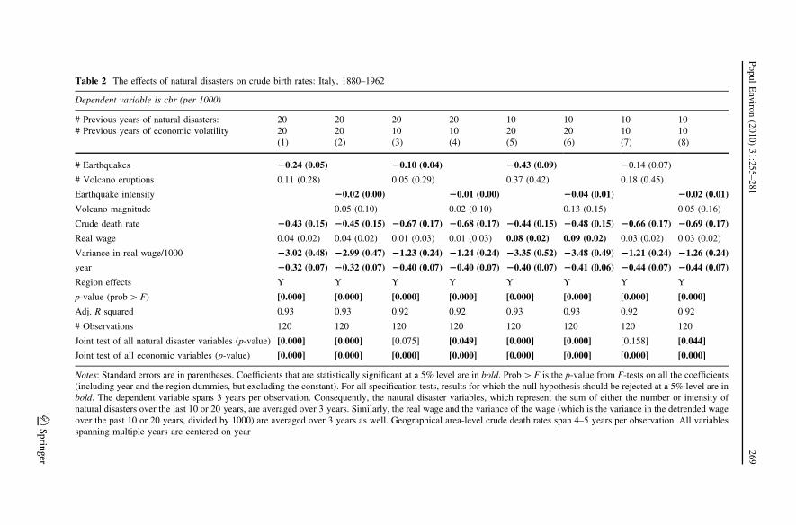
Table 2 The effects of natural disasters on crude birth rates: Italy, 1880–1962

Dependent variable is cbr (per 1000)

# Previous years of natural disasters: 20 20 20 20 10 10 10 10

# Previous years of economic volatility 20 20 10 10 20 20 10 10

(1) (2) (3) (4) (5) (6) (7) (8)

# Earthquakes 20.24 (0.05) 20.10 (0.04) 20.43 (0.09) 20.14 (0.07)

# Volcano eruptions 0.11 (0.28) 0.05 (0.29) 0.37 (0.42) 0.18 (0.45)

Earthquake intensity 20.02 (0.00) 20.01 (0.00) 20.04 (0.01) 20.02 (0.01)

Volcano magnitude 0.05 (0.10) 0.02 (0.10) 0.13 (0.15) 0.05 (0.16)

Crude death rate 20.43 (0.15) 20.45 (0.15) 20.67 (0.17) 20.68 (0.17) 20.44 (0.15) 20.48 (0.15) 20.66 (0.17) 20.69 (0.17)

Real wage 0.04 (0.02) 0.04 (0.02) 0.01 (0.03) 0.01 (0.03) 0.08 (0.02) 0.09 (0.02) 0.03 (0.02) 0.03 (0.02)

Variance in real wage/1000 23.02 (0.48) 22.99 (0.47) 21.23 (0.24) 21.24 (0.24) 23.35 (0.52) 23.48 (0.49) 21.21 (0.24) 21.26 (0.24)

year 20.32 (0.07) 20.32 (0.07) 20.40 (0.07) 20.40 (0.07) 20.40 (0.07) 20.41 (0.06) 20.44 (0.07) 20.44 (0.07)

Region effects Y Y Y Y Y Y Y Y

p-value (prob [ F) [0.000] [0.000] [0.000] [0.000] [0.000] [0.000] [0.000] [0.000]

Adj. R squared 0.93 0.93 0.92 0.92 0.93 0.93 0.92 0.92

# Observations 120 120 120 120 120 120 120 120

Joint test of all natural disaster variables (p-value) [0.000] [0.000] [0.075] [0.049] [0.000] [0.000] [0.158] [0.044]

Joint test of all economic variables (p-value) [0.000] [0.000] [0.000] [0.000] [0.000] [0.000] [0.000] [0.000]

Notes: Standard errors are in parentheses. Coefficients that are statistically significant at a 5% level are in bold. Prob [ F is the p-value from F-tests on all the coefficients

(including year and the region dummies, but excluding the constant). For all specification tests, results for which the null hypothesis should be rejected at a 5% level are in

bold. The dependent variable spans 3 years per observation. Consequently, the natural disaster variables, which represent the sum of either the number or intensity of

natural disasters over the last 10 or 20 years, are averaged over 3 years. Similarly, the real wage and the variance of the wage (which is the variance in the detrended wage

over the past 10 or 20 years, divided by 1000) are averaged over 3 years as well. Geographical area-level crude death rates span 4–5 years per observation. All variables

spanning multiple years are centered on year

Po

pu

lE

nv

iron

(20

10

)3

1:2

55

–2

81

26

9

123

coefficients. Once again, the disaster variables are jointly significant, and the

economic variables are jointly significant. Earthquakes, earthquake intensity, and

economic volatility continue to have a significant negative association with the

crude birth rate even when the number of previous years of either disasters or

economic volatility, or both, is changed from 20 to 10.16

The results for the crude birth rate in Italy show that short-run instability doesaffect fertility behavior. However, the effect is the opposite of the one that would

occur as predicted by Jones (1981) as a result of long-run steady-state instability.

According to Jones (1981), who hypothesized that families living in a more natural

disaster-prone environment would accumulate a population surplus as a form of

demographic insurance against catastrophe, one would expect natural disasters to

have a positive effect on fertility. Instead, the results suggest that individuals react

to natural disasters by decreasing, not increasing, their fertility, perhaps because the

shock makes individuals less willing to make the long-term investments required to

raise a family. The direction of the result is thus consistent with the hypothesis that

individuals respond to short-run instability by decreasing such long-term invest-

ments as bearing and raising children.

In addition to natural disasters, a second form of short-run instability considered

is economic volatility, as measured by the variance of the detrended wage. Although

economic theory predicts that greater economic volatility will lower investment in

human and physical capital (Blattman et al. 2007), it is agnostic about its effects on

fertility. The empirical results of this article suggest that, just as with environmental

instability, individuals react to volatile wages by decreasing their fertility. The

direction of the result is also consistent with the hypothesis that individuals respond

to short-run instability by decreasing such long-term investments as bearing and

raising children.

Are the results for the crude birth rate robust to other measures of fertility in

Italy? As seen in Table 3, which presents the results from the base case using 20

previous years for both environmental shocks and economic volatility, the

significant negative coefficients in the base case models 1 and 2 of Table 2 on

either earthquake number or earthquake intensity and on the variance in the wage, as

well the joint significance of the disaster and economic variables, respectively, also

hold for both total fertility and marital fertility as well. Non-marital fertility is

affected only by the number of earthquakes, and not by the earthquake intensity or

economic volatility.

Table 4 reports the results when geographical area–year interactions are included

to control for all other factors other than natural disasters that vary by locality and

time, including local economic shocks and local mortality. When geographical

area–year interactions are included, natural disasters are no longer significant for

either the crude birth rate or total fertility, but both the number and the intensity of

earthquakes have a significant negative effect on marital fertility. For non-marital

fertility, the number of earthquakes has a significant positive effect, which may

explain why the net effect of earthquakes on total fertility is insignificant, and the

16 The exception is that when only 10 previous years are considered for both disasters and economic

volatility (model 7), disasters no longer have a significant effect.

270 Popul Environ (2010) 31:255–281

123

Table 3 The effects of natural disasters on fertility: Italy, 1880–1962

Dependent variable

Total fertility If Marital fertility Ig Non-marital fertility Ih

(1) (2) (3) (4) (5) (6)

# Earthquakes 20.44 (0.06) 20.89 (0.13) 20.06 (0.03)

# Volcano eruptions 0.17 (0.34) 0.68 (0.69) 20.13 (0.16)

Earthquake intensity 20.04 (0.01) 20.08 (0.01) 20.00 (0.00)

Volcano magnitude 0.09 (0.11) 0.25 (0.23) 20.03 (0.06)

Crude death rate 20.52 (0.18) 20.54 (0.18) 21.71 (0.38) 21.76 (0.37) 20.11 (0.09) 20.11 (0.09)

Real wage 0.02 (0.03) 0.02 (0.03) 0.01 (0.06) 0.00 (0.06) 20.00 (0.01) 0.00 (0.01)

Variance in real wage/1000 24.24 (0.58) 24.19 (0.56) 29.57 (1.18) 29.55 (1.14) 20.42 (0.28) 20.36 (0.28)

Year 20.28 (0.08) 20.28 (0.08) 20.57 (0.17) 20.56 (0.17) 20.07 (0.04) 20.07 (0.04)

Region effects Y Y Y Y Y Y

p-value (prob [ F) [0.000] [0.000] [0.000] [0.000] [0.000] [0.000]

Adj. R squared 0.92 0.92 0.89 0.90 0.65 0.64

# Observations 120 120 120 120 120 120

Joint test of all natural disaster variables (p-value) [0.000] [0.000] [0.000] [0.000] [0.082] [0.161]

Joint test of all economic variables (p-value) [0.000] [0.000] [0.000] [0.000] [0.317] [0.430]

Notes: Standard errors are in parentheses. Coefficients that are statistically significant at a 5% level are in bold. Prob [ F is the p-value from F-tests on all the coefficients

(including year and the region dummies, but excluding the constant). For all specification tests, results for which the null hypothesis should be rejected at a 5% level are in

bold. Each dependent variable spans 3 years per observation. Consequently, the natural disaster variables, which represent the sum of either the number or intensity of

natural disasters over the last 20 years, are averaged over 3 years. Similarly, the real wage and the variance of the wage (which is the variance in the detrended wage over

the past 20 years, divided by 1000) are averaged over 3 years as well. Geographical area-level crude death rates span 4–5 years per observation. All variables spanning

multiple years are centered on year

Po

pu

lE

nv

iron

(20

10

)3

1:2

55

–2

81

27

1

123

number of volcano eruptions has a significant negative effect, but, because the

p-value on the joint test of the number of natural disasters is higher and because

neither earthquake intensity nor volcano magnitude has a significant effect, the

effects of natural disasters on non-marital fertility are weaker than they are on

marital fertility.

Taken together, the results using the regional data for Italy provide strong

evidence that fertility behavior is negatively associated with environmental shocks

and short-run economic volatility. The channel through which this occurs appears to

be marital fertility: married couples who experienced natural disasters and volatile

wages over the previous two decades will tend to have fewer children.

As seen in the results of the spatial lag model in Table 5, natural disasters

continue to have a significant negative association with the crude birth rate even

when spatial spillovers are taken into account. When region fixed effects are used,

economic volatility is negatively associated with the crude birth rate as well. Thus,

Table 4 The effects of natural disasters on fertility using geographical area–year interactions: Italy,

1820–1962

Dependent variable

cbr (per 1000) Total fertility If Marital fertility

IgNon-marital

fertility Ih

(1) (2) (3) (4) (5) (6) (7) (8)

# Earthquakes 20.16

(0.20)

20.15

(0.24)

20.96(0.48)

0.27(0.11)

# Volcano eruptions 20.07

(0.12)

20.09

(0.14)

20.18

(0.28)

20.13(0.06)

Earthquake intensity 20.02

(0.02)

20.01

(0.03)

20.12(0.06)

0.02

(0.01)

Volcano magnitude 20.02

(0.04)

20.04

(0.05)

20.03

(0.10)

20.04

(0.02)

Geographical area effects Y Y Y Y Y Y Y Y

year effects Y Y Y Y Y Y Y Y

Geographical area—year

effects

Y Y Y Y Y Y Y Y

p-value (Prob [ F) [0.000] [0.000] [0.000] [0.000] [0.000] [0.000] [0.000] [0.000]

Adj. R squared 0.90 0.90 0.90 0.90 0.86 0.86 0.64 0.63

# Observations 212 212 184 184 184 184 184 184

Joint test of all natural

disaster variables (p-

value)

[0.344] [0.319] [0.368] [0.410] [0.012] [0.015] [0.041] [0.183]

Notes: Standard errors are in parentheses. Fertility indices are multiplied by 100. Coefficients that are

statistically significant at a 5% level are in bold. Prob [ F is the p-value from F-tests on all the coef-

ficients (excluding the constant). For all specification tests, results for which the null hypothesis should be

rejected at a 5% level are in bold. Each dependent variable spans 3 years per observation. Consequently,

the natural disaster variables, which represent the sum of either the number or intensity of natural

disasters over the last 20 years, are averaged over 3 years. All variables spanning multiple years are

centered on year

272 Popul Environ (2010) 31:255–281

123

the negative association of natural disasters and economic volatility with fertility is

robust to spatial effects.

The story is somewhat different for Japan, as seen in Table 6. When 20 previous

years of natural disasters are considered, the number of tsunamis has a significant

negative association with the crude birth rate. In the base case (model 1), an

additional tsunami in the previous 20 years decreases the crude birth rate by 246

births per 100,000 people. Relative to the mean crude birth rate for Japan over this

time period (1727–1935) of 29.07 per 1000, this is a 8.46% decrease. Tsunamis no

longer have a significant effect when only 10 previous years of natural disasters is

used instead of 20. Tsunami magnitude has no significant effect on fertility. Neither

volcano eruptions or earthquakes have a significant effect on fertility in any of the

models. Unlike for Italy, economic volatility does not have any effect in any of the

models.

Table 7 reports the results when region–year interactions are included to control

for all the factors other than natural disasters that vary by locality and time,

including local economic shocks. When geographical area–year interactions are

included, tsunamis continue to have a negative effect on fertility, this time both in

number and magnitude. Unlike before, earthquakes have a significant positive effect

on fertility, both in number and magnitude. As before, the crude death rate has no

significant effect.

The results that natural disasters still have a significant effect on fertility even

after controlling for local time-varying effects such as local mortality and local

wages suggests that natural disasters in of themselves affect fertility, even when

Table 5 The effects of natural disasters on crude birth rates using a spatial lag model: Italy, 1880–1962

Dependent variable is cbr (per 1000)

(1) (2) (3) (4)

# Earthquakes 20.33 (0.10) 20.21 (0.05)

# Volcano eruptions 0.31 (0.49) 20.62 (0.60)

Earthquake intensity 20.04 (0.01) 20.02 (0.00)

Volcano magnitude 0.10 (0.16) 20.14 (0.18)

Crude death rate 0.85 (0.25) 20.31 (0.14) 0.73 (0.24) 20.32 (0.14)

Real wage 20.04 (0.05) 0.03 (0.02) 0.05 (0.05) 0.03 (0.02)

Variance in real wage/1000 23.68 (1.02) 22.75 (0.52) 24.13 (0.98) 22.76 (0.51)

year 0.19 (0.13) 20.26 (0.07) 0.19 (0.12) 0.26 (0.07)

Region effects N Y N Y

q 0.01 (0.01) 0.04 (0.02) 0.01 (0.01) 0.04 (0.02)

# Observations 106 106 106 106

Notes: Standard errors are in parentheses. Coefficients that are statistically significant at a 5% level are in

bold. The dependent variable spans 3 years per observation. Consequently, the natural disaster variables,

which represent the sum of either the number or intensity of natural disasters over the last 20 years, are

averaged over 3 years. Similarly, the real wage and the variance of the wage (which is the variance in the

detrended wage over the past 20 years, divided by 1000) are averaged over 3 years as well. Geographical

area-level crude death rates span 4–5 years per observation. All variables spanning multiple years are

centered on year

Popul Environ (2010) 31:255–281 273

123

Table 6 The effects of natural disasters on crude birth rates: Japan, 1737–1935

Dependent variable is cbr (per 1000)

# Previous years of natural disasters: 20 20 20 20 10 10 10 10# Previous years of economic volatility 20 20 10 10 20 20 10 10

(1) (2) (3) (4) (5) (6) (7) (8)

# Earthquakes 0.86 (1.73) 20.67 (1.71) 1.90 (2.06) 1.62 (2.20)

# Tsunamis 22.46 (1.21) 22.76 (1.12) 22.43 (1.75) 22.81 (1.80)

# Volcano eruptions 0.90 (0.84) 0.86 (0.84) 2.50 (1.80) 2.32 (1.81)

Earthquake magnitude 20.14 (0.40) 20.15 (0.41) 20.64 (0.57) 20.51 (0.57)

Tsunami magnitude 20.48 (0.38) 20.55 (0.36) 20.04 (0.52) 20.24 (0.53)

Volcano magnitude 0.24 (0.28) 0.23 (0.28) 0.46 (0.57) 0.39 (0.57)

Crude death rate 20.02 (0.10) 20.01 (0.10) 20.02 (0.10) 20.01 (0.10) 20.04 (0.10) 20.02 (0.10) 20.03 (0.10) 20.01 (0.10)

Real wage 0.07 (0.16) 0.06 (0.16) 0.03(0.16) 0.04 (0.16) 0.10 (0.16) 0.12 (0.17) 25.35 (53.81) 0.03 (0.17)

Variance in real wage/1000 31.17 (45.37) 27.35 (45.26) 10.21 (46.23) 7.95 (46.90) 61.61 (44.05) 63.58 (42.90) 11.66 (50.06)

year 20.02 (0.05) 20.01 (0.04) 20.00 (0.05) 0.01 (0.04) 20.04 (0.05) 20.03 (0.04) 20.01 (0.05) 0.00 (0.04)

Place effects Y Y Y Y Y Y Y Y

p-value (Prob [ F) [0.000] [0.000] [0.000] [0.000] [0.000] [0.000] [0.000] [0.000]

Adj. R squared 0.50 0.50 0.50 0.50 0.50 0.49 0.49 0.48

# Observations 146 146 146 146 146 146 146 146

Joint test of all natural disastervariables (p-value)

[0.131] [0.185] [0.069] [0.095] [0.233] [0.354] [0.218] [0.391]

Joint test of all economicvariables (p-value)

[0.782] [0.819] [0.966] [0.969] [0.300] [0.334] [0.895] [0.966]

Notes: Standard errors are in parentheses. Coefficients that are statistically significant at a 5% level are in bold. Prob [ F is the p-value from F-tests on all the coefficients(including year and the region dummies, but excluding the constant). For all specification tests, results for which the null hypothesis should be rejected at a 5% level are inbold. Crude birth rates span 1–41 years per observation, with an average span of approximately 10 years. Consequently, the natural disaster variables, which represent thesum of either the number or intensity of natural disasters over the last 10 or 20 years, are averaged over 10 years. Similarly, the real wage and the variance of the wage(which is the variance in the detrended wage over the past 10 or 20 years, divided by 1000) are averaged over 10 years as well. Crude death rates span the same number ofyears as the crude birth rate for each observation. All variables spanning multiple years are centered on year

27

4P

op

ul

En

viro

n(2

01

0)

31

:25

5–

28

1

123

controlling for its effect on the wage and on mortality. Natural disasters do not

simply operate through disaster-induced reductions in income or through disaster-

induced mortality. In order to further investigate whether natural disasters operate

through the mortality channel alone, I aggregated the crude death rates over the

previous 20 years and used that variable instead of the number of natural disasters

over the previous 20 years. The results are presented in Table 8. The coefficient on

the crude death rate over the previous 20 years is not significant for either Italy or

Japan. As with the previous results with the natural disaster regressions, the

coefficient on the variance of the wage over the previous 20 years is significant and

negative for Italy. The insignificant coefficients on the crude death rate over the

previous 20 years may be because the crude death rate is a noisy measure of the

number of deaths due to disasters, and because individual fertility may respond to

the other disruptions resulting from the natural disaster than death alone. Thus,

natural disasters have an effect on fertility that extends beyond its effect on

mortality. Mortality is not the only channel from natural disasters to fertility.

The results, therefore, show that natural disasters have a significant negative

association with fertility in Italy and a significant negative effect for tsunamis and

Table 7 The effects of natural disasters on crude birth rates using region–year interactions: Japan, 1671–

1965

Dependent variable is cbr (per 1000)

(1) (2)

# Earthquakes 4.64 (1.76)

# Tsunamis 212.17 (2.82)

# Volcano eruptions 20.38 (1.42)

Earthquake magnitude 0.86 (0.35)

Tsunami magnitude 22.14 (0.66)

Volcano magnitude 20.09 (0.36)

Crude death rate 0.24 (0.14) 0.24 (0.14)

Region effects Y Y

year effects Y Y

Region—year effects Y Y

p-value (prob [ F) [0.000] [0.000]

Adj. R squared 0.89 0.89

# Observations 165 165

Joint test of all natural disaster variables (p-value) [0.004] [0.051]

Notes: Standard errors are in parentheses. Coefficients that are statistically significant at a 5% level are in

bold. Prob [ F is the p-value from F-tests on all the coefficients (excluding the constant). For all

specification tests, results for which the null hypothesis should be rejected at a 5% level are in bold. Crude

birth rates span 1–41 years per observation, with an average span of approximately 10 years. Conse-

quently, the natural disaster variables, which represent the sum of either the number or intensity of natural

disasters over the last 20 years, are averaged over 10 years. Crude death rates span the same number of

years as the crude birth rate for each observation. All variables spanning multiple years are centered on

year

Popul Environ (2010) 31:255–281 275

123

positive effect for earthquakes in Japan. Short-run economic volatility has negative

associations with fertility in Italy, but not in Japan. Thus, at least in Italy, short-run

instability, particularly that arising from the natural environment, is associated with

lower investment in the population size of future generations.

Concluding remarks

The research in this article presents a detailed investigation of the effects of

environmental and economic instability on fertility and its components in both Italy

and Japan. For identification, regional data are used to exploit the natural variation

within each of these two countries.

Three results deserve special mention. First, environmental shocks have a

significant association with fertility behavior in both countries, even after

controlling for year, the death rate, the wage, short-run economic volatility, and

steady-state risk. The sign of the association varies by country and disaster type. In

Italy, earthquakes had a robust negative association with fertility, particularly

marital fertility. In Japan, tsunamis had a robust negative association with fertility,

while earthquakes had a significant positive association with fertility in some

specifications.

Table 8 The effects of mortality on crude birth rates in Italy (1880–1962) and Japan (1737–1935)

Dependent variable is cbr (per 1000)

Country Italy Japan

# Previous years of economic volatility 20 20

(1) (2)

Crude death rate over previous 20 years 20.04 (0.03) 0.00 (0.01)

Contemporaneous crude death rate 20.35 (0.17) 20.02 (0.10)

Real wage 0.05 (0.03) 0.04 (0.17)

Variance in real wage over previous 20 years/1000 21.69 (0.40) 64.12 (43.94)

Year 20.38 (0.07) -0.03 (0.04)

Region or place effects Y Y

p-value (prob [ F) [0.000] [0.000]

Adj. R squared 0.91 0.49

# Observations 120 146

Joint test of all economic variables (p-value) [0.000] [0.296]

Notes: Standard errors are in parentheses. Coefficients that are statistically significant at a 5% level are in

bold. Prob [ F is the p-value from F-tests on all the coefficients (including year and the region dummies,

but excluding the constant). For all specification tests, results for which the null hypothesis should be

rejected at a 5% level are in bold. The crude birth rate variable spans 3 years per observation for Italy and

1–41 years with an average span of approximately 10 years for Japan. Consequently, the real wage and

the variance of the wage (which is the variance in the detrended wage over the past 20 years, divided by

1000) are averaged over 3 years for Italy and 10 years for Japan. For Italy, geographical area-level crude

death rates span 4–5 years per observation. For Japan, rude death rates span the same number of years as

the crude birth rate for each observation. All variables spanning multiple years are centered on year

276 Popul Environ (2010) 31:255–281

123

A second important result is that short-run economic volatility, as measured by

the variance of the detrended wage, has a significant negative association with

fertility in Italy. Taken together, the significant negative association between short-

run instability and fertility behavior in Italy suggest that, just as economic instability

decreases investment in physical and human capital, environmental shocks and

economic volatility are associated with a decrease in investment in the population

size of future generations.

These results have many important implications. First, the results have

implications for understanding differences in income and population growth both

within and between countries and both throughout the past and in the present.

Second, they have implications for policies regarding disaster insurance, foreign aid,

and the environment. Third, these results have important implications for the

development of models of behavior under uncertainty. Fourth, the results have

implications for the design of policies for risk-sharing. If natural disasters cause a

decrease in fertility because they make families reluctant to invest in having

children, then risk-sharing policies such as disaster insurance can help mitigate

these effects. Moreover, in countries such as Italy where economic volatility is

associated with a decline in fertility, policies such as foreign aid or prohibitions

against cutting wages that minimize the volatility can attenuate the impact on

fertility. These policies can be the subject of future research.

The third important result is that, just as there are differences in how fertility

rates in Italy and Japan respond to natural disasters, there are systematic differences

in how fertility rates in these two countries respond economic volatility. The

variance in the detrended wage has a negative association on the crude birth rate,

total fertility and marital fertility in Italy, but an insignificant effect on the crude

birth rate in Japan. One possible reason why the fertility choices of the Japanese

respond less to economic volatility than do those of the Italians is that there may be

some institutions in Japan, such as cultural norms, that already provide the Japanese

with insurance against economic volatility. Another possible reason is that, as seen

in the summary statistics in Table 1, the Japanese wage appears less volatile than

the Italian wage, and thus may be too stable to have much of an effect of fertility.

The different effects of natural disasters and economic volatility on Italy versus

Japan highlight the importance of country-specific factors such as social attitudes,

cultural values, network behavior, history, politics, and people’s fertility prefer-

ences. Contrary to Jones’ (1981) theory, differences in fertility between Italy and

Japan cannot be explained away by disaster proneness alone. These other factors

vary by country, and are likely to be different for other countries in Asia and Europe

as well.

The main results are, therefore, that natural disasters have a significant

association with fertility in both countries. In Italy, earthquakes had a robust

negative association with fertility, particularly marital fertility. In Japan, tsunamis

had a robust negative association with fertility while earthquakes had a significant

positive association with fertility in some specifications. Short-run economic

volatility has a significant negative association with fertility in Italy but no

association in Japan. These results should be of interest to economists, historians,

environmentalists, and policymakers alike.

Popul Environ (2010) 31:255–281 277

123

Acknowledgment I would like to thank Jeffrey Williamson for his advice and guidance throughout this

project. I also benefited from discussions with Oded Galor, Claudia Goldin, Jerry Green, Lori Hunter,

Dale Jorgenson, Michael Kremer, Satomi Kurosu, Ronald Lee, Lant Pritchett, Mark Rosenzweig,

Amartya Sen, Robert Stavins, and Kip Viscusi. Participants at workshops in economic development and

in economic history at Harvard University provided helpful comments. Countless individuals provided

invaluable assistance during the data collection process, most notably Susan Hanley and James Z. Lee. I

received financial support from an EPA Science to Achieve Results graduate fellowship, a National

Science Foundation graduate research fellowship, and a Repsol YPF–Harvard Kennedy School Pre-

Doctoral Fellowship in energy policy. All errors are my own.

Open Access This article is distributed under the terms of the Creative Commons Attribution Non-

commercial License which permits any noncommercial use, distribution, and reproduction in any med-

ium, provided the original author(s) and source are credited.

Appendix 1

See Table 9.

Appendix 2

See Table 10.

Table 9 Raw data for Italy, 1820–1962

Variable Source

Regional variables

Crude birth rate (per 1000) Livi-Bacci 1977, pp. 22–23 and 62

Total fertility index If Treadway 1980

Marital fertility index Ig Treadway 1980

Non-marital fertility index Ih Treadway 1980

Natural disaster variables

# Earthquakes Dunbar et al. 1999

Earthquake intensity (Modified Mercalli Intensity) Dunbar et al. 1999

# Volcano eruptions Whiteside 1999

Volcano magnitude (volcano explosivity index ? 1) Whiteside 1999

Geographical area-level variables

Crude death rate (per 1000) Del Panta 1979, p. 226

National variables

Real wage (1900 = 100) Williamson 1995

278 Popul Environ (2010) 31:255–281

123

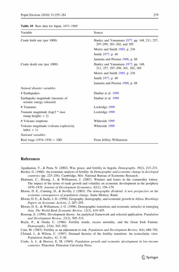
References

Agadjanian, V., & Prata, N. (2002). War, peace, and fertility in Angola. Demography, 39(2), 215–231.

Becker, G. (1960). An economic analysis of fertility. In Demographic and economic change in developedcountries (pp. 225–256). Cambridge, MA: National Bureau of Economic Research.

Blattman, C., Hwang, J., & Williamson, J. (2007). Winners and losers in the commodity lottery:

The impact of the terms of trade growth and volatility on economic development in the periphery

1870–1939. Journal of Development Economics, 82(1), 156–179.

Bloom, D. E., Canning, D., & Sevilla, J. (2003). The demographic dividend: A new perspective on theeconomic consequences of population change. Santa Monica: Rand.

Bloom, D. E., & Sachs, J. D. (1998). Geography, demography, and economic growth in Africa. BrookingsPapers on Economic Activity, 2, 207–295.

Bloom, D. E., & Williamson, J. G. (1998). Demographic transitions and economic miracles in emerging

Asia. The World Bank Economic Review, 12(3), 419–455.

Boserup, E. (1996). Development theory: An analytical framework and selected application. Populationand Development Review, 22(3), 505–515.

Boyle, P., & Grada, C. (1986). Fertility trends, excess mortality, and the Great Irish Famine.

Demography, 23(4), 543–562.

Cain, M. (1983). Fertility as an adjustment to risk. Population and Development Review, 9(4), 688–702.

Cleland, J., & Wilson, C. (1987). Demand theories of the fertility transition: An iconoclastic view.

Population Studies, 41, 5–30.

Coale, A. J., & Hoover, E. M. (1969). Population growth and economic development in low-incomecountries. Princeton: Princeton University Press.

Table 10 Raw data for Japan, 1671–1965

Variable Source

Crude birth rate (per 1000) Hanley and Yamamura 1977, pp. 148, 211, 257,

297–299, 301–302, and 305

Morris and Smith 1985, p. 236

Smith 1977, p. 40

Jannetta and Preston 1998, p. 88

Crude death rate (per 1000) Hanley and Yamamura 1977, pp. 148,

211, 257, 297–299, 301, 302, 305

Morris and Smith 1985, p. 236

Smith 1977, p. 40

Jannetta and Preston 1998, p. 88

Natural disaster variables

# Earthquakes Dunbar et al. 1999

Earthquake magnitude (measure of

seismic energy released)

Dunbar et al. 1999

# Tsunamis Lockridge 1999

Tsunami magnitude (log(2 * max

runup height) ? 2)

Lockridge 1999

# Volcano eruptions Whiteside 1999

Volcano magnitude (volcano explosivity

index ? 1)

Whiteside 1999

National variables

Real wage (1934–1936 = 100) From Jeffrey Williamson

Popul Environ (2010) 31:255–281 279

123

del Panta, L. (1979). Italy. In W. Lee (Ed.), European demography and economic growth (pp. 196–235).

New York: St. Martin’s Press.

Diamond, J. (1997). Guns, germs, and steel. New York: W. W. Norton & Company.

Dunbar, P., Lockridge, P., & Whiteside, L. (1999). National geophysical data center [NGDC] significant

earthquake database. Cited June 22, 2002. ftp://ftp.ngdc.noaa.gov/Solid_Earth/Natural_Hazards/

Seismicity/Signif_EQ/.

Dyson, T. (1991). On the demography of South Asian famines part II. Population Studies, 45, 279–297.

Frankenberg, E., Beegle, K., Thomas, D., & Suriastini, W. (1999). Health, education and the economic

crisis in Indonesia (Working paper, University of California at Los Angeles). http://chd.ucla.edu/

IFLS/ppr/edhltxt.pdf.

Gallup, J., Sachs, J., & Mellinger, A. (1999). Geography and economic development. InternationalRegional Science Review, 22, 179–232.

Galor, O. (2004). The demographic transition and the emergence of sustained economic growth (Working

paper, Brown University).

Hanley, S., & Yamamura, K. (1977). Economic and demographic change in preindustrial Japan 1600–1868. Princeton: Princeton University Press.

Heuveline, P., & Poch, B. (2007). The phoenix population: Demography crisis and rebound in Cambodia.

Demography, 44(2), 405–426.

Hoffman, E. (1981). The sources of mortality changes in Italy since unification. New York: Arno Press.

Jannetta, A., & Preston, S. (1998). Two centuries of mortality change in central Japan: The evidence from

a temple death register. In M. Smitka (Ed.), Historical demography and labor markets in prewarJapan (pp. 79–99). New York: Garland Publishing, Inc.

Jones, E. (1981). The European miracle. Cambridge: Cambridge University Press.

Kalipeni, E. (1996). Demographic response to environmental pressure in Malawi. Population andEnvironment, 17(4), 285–308.

Kohler, H. -P., Billari, F. C., & Ortega, J. A. (2002). The emergence of lowest-low fertility in Europe

during the 1990s. Population and Development Review, 28, 641–680.

Lee, R. (1973). Population in preindustrial England: An econometric analysis. Quarterly Journal ofEconomics, 87(4), 581–607.

Lee, R. (1985). Population homeostasis and English demographic history. Journal of InterdisciplinaryHistory, 15(4), 635–660.

Lee, R., & Edwards, R. (2001). The fiscal impact of population change. In J. S. Little & R. K. Triest

(Eds.), Seismic shifts: The economic impact of demographic change (Federal Reserve Bank of

Boston conference series no. 46) pp. 220–237.

Lee, J., & Wang, F. (1999). One quarter of humanity: Malthusian mythology and Chinese realities: 1700–2000. Cambridge, MA: Harvard University Press.

Lin, C.- Y. C. (2004). The effects of natural disasters and economic volatility on fertility (Working paper

(distributed via SSRN), Harvard University). http://ssrn.com/abstract=590421.

Lindahl-Kiessling, K., & Landberg, H. (Eds.). (1994). Population, economic development, and theenvironment. Oxford: Oxford University Press.

Livi-Bacci, M. (1977). A history of Italian fertility during the last two centuries. Princeton: Princeton

University Press.

Lockridge, P. (1999). National geophysical data center [NGDC] tsunami database. Cited June 22, 2002.

ftp://ftp.ngdc.noaa.gov/Solid_Earth/Natural_Hazards/Tsunami/.

Madhavan, S., Adams, A., & Simon, D. (2003). Women’s networks and the social world of fertility

behavior. International Family Planning Perspectives, 29(2), 58–68.

Maharatna, A. (1996). The demography of famines. Oxford: Oxford University Press.

Mason, A. (1997). The response of fertility and mortality to economic crisis and structural adjustment

policy during the 1980s: A review. In G. P. Tapinos, A. Mason, & J. Bravo (Eds.), Demographicresponses to economic adjustment in Latin America (pp. 17–34). Oxford: Oxford University Press.

Morris, D., & Smith, T. (1985). Fertility and mortality in an outcaste village in Japan, 1750–1869. In S.

Hanley & A. Wolf (Eds.), Family and population in East Asian history (pp. 229–246). Stanford:

Stanford University Press.

Munshi, K., & Myaux, J. (2006). Social norms and the fertility transition. Journal of DevelopmentEconomics, 80, 1–38.

National Bureau of Economic Research [NBER]. (1960). Demographic and economic change indeveloped countries. Princeton: Princeton University Press.

Pebley, A. R. (1998). Demography and the environment. Demography, 35(4), 377–389.

280 Popul Environ (2010) 31:255–281

123

Perelli-Harris, B. (2005). The path to lowest-low fertility in Ukraine. Population Studies, 59(1), 55–70.

Portner, C. C. (2006). Gone with the wind?: Hurricance risk, fertility and education. (Working paper,

University of Washington).

Ramey, G., & Ramey, V. R. (1995). Cross-country evidence on the link between volatility and growth.

The American Economic Review, 85(5), 1138–1151.

Rosenzweig, M., & Wolpin, K. (1993). Credit market constraints, consumption smoothing, and the

accumulation of durable production assets in low-income countries: Investments in bullocks in

India. Journal of Political Economy, 101(2), 223–244.

Sachs, J. (2001). Tropical underdevelopment. NBER working paper series (Working Paper No. 8119,

Cambridge, MA).

Schofield, R., & Wrigley, E. (1985). Population and economy: From the traditional to the modern world.

Journal of Interdisciplinary History, 15(4), 561–569.

Smith, T. (1977). Nakahara: Family farming and population in a Japanese village, 1717–1830. Stanford:

Stanford University Press.

Spengler, J. J. (1969). Economics and demography. In P. M. Hauser & O. D. Duncan (Eds.), The study ofpopulation. Chicago: University of Chicago Press.

Stavig, G. R. (1979). The impact of population growth on the economy of countries. EconomicDevelopment and Cultural Change, 27(4), 735–750.

Thomas, D., Beegle, K., Frankenberg, E., Sikoki, B., Strauss, J., & Teruel, G. (2004). Education in a

crisis. Journal of Development Economics, 74(1), 53–85.

Thomson, E., & Goldman, P. (1987). Measuring fertility norms. Population and Environment, 9(3),

173–185.

Treadway, R. (1980). Princeton European fertility project: Demographic data. Cited June 7, 2002.

http://opr.princeton.edu/archive/eufert/demog.html.

Walford, C. (1970). The famines of the world, past and present. New York: B. Franklin.

Whiteside, L. (1999). National geophysical data center [NGDC] volcano database. Cited June 22, 2002.

ftp://ftp.ngdc.noaa.gov/Solid_Earth/Natural_Hazards/volcano/.

Williamson, J. (1995). The evolution of global labor markets since 1830: Background evidence and

hypotheses. Explorations in Economic History, 32, 141–196.

Willis, R. J. (1973). A new approach to the economic theory of fertility behavior. The Journal of PoliticalEconomy, 81(2), S14–S64.

Wooldridge, J. (2002). Econometric analysis of cross section and panel data. Cambridge: MIT Press.

Popul Environ (2010) 31:255–281 281

123