RHEINISCH-WESTFÄLISCHE TECHNISCHE HOCHSCHULE AACHEN

Institut fur Mathematik

Energetics and dynamics of globalintegrals modeling interaction

between stiff filaments

by

Philipp ReiterDieter Felix

Heiko von der MoselWolfgang Alt

Report No. 21 2008

April 2008

Institute for Mathematics, RWTH Aachen University

Templergraben 55, D-52062 AachenGermany

Energetics and dynamics of global integrals modeling

interaction between stiff filaments

Philipp Reiter, Dieter Felix, Heiko von der Mosel, Wolfgang Alt

April 21, 2008

Abstract

The attractive and spacing interaction between pairs of filaments viacross-linkers, e.g. myosin dimers connecting actin filaments, is modeledby global integral kernels for negative binding energies between two in-tersecting stiff and long rods in a (projected) 2-dimensional situation, forsimplicity. Whereas maxima of the global energy functional represent in-tersection angles of ‘minimal contact’ between the filaments, minima areapproached for energy values tending to −∞, representing the two de-generate states of parallel and anti-parallel filament alignment. Standarddifferential equations of negative gradient flow for such energy functionalsshow convergence of solutions to one of these degenerate equilibria in finitetime, thus called ‘super-stable’ states.

By considering energy variations under virtual rotation or translationof one filament with respect to the other, integral kernels for the resultinglocal forces parallel and orthogonal to the filament are obtained. Forthe special modeling situation that these variations only activate ‘springforces’ in direction of the cross-links, explicit formulas for total torque andtranslational forces are given and calculated for typical examples. Again,the two degenerate alignment states are locally ‘super-stable’ equilibriaof the assumed over-damped dynamics, but also other stable states oforthogonal arrangement and different asymptotic behavior can occur.

These phenomena become apparent if stochastic perturbations of thelocal force kernels are implemented as additive Gaussian noise inducedby the cross-link binding process with appropriate scaling. Then globalfilament dynamics is described by a certain type of degenerate stochas-tic differential equations yielding asymptotic stationary processes aroundthe alignment states, which have generalized, namely bimodal Gaussiandistributions. Moreover, stochastic simulations reveal characteristic slid-ing behavior as it is observed for myosin-mediated interaction betweenactin filaments. Finally, the forgoing explicit and asymptotic analysis aswell as numerical simulations are extended to the more realistic modelingsituation with filaments of finite length.

KeywordsActin filaments · Polymer cross-linking · Myosin dimers · Interaction energy ·Knot energies · Filament alignment · Torque · Stochastic differential equations· Generalized Gauss distributions

1

1 Introduction

Contact avoidance of a closed curve Γ in 3-dimensional space (like a cyclic poly-mer, for example, certain modified DNA strands) can be modeled by defininga global knot energy. According to [17], Def. 1.1, a real-valued functional onthe space of knots is called a knot energy, if it is bounded from below and self-repulsive, i. e. blows up on sequences of embedded curves converging to a curvewith a self-intersection. A large family of knot energies may be represented byglobal integrals of the form

EΓ =

∫

Γ

∫

ΓHrep

(γ(s) − γ(s), γ′(s), γ′(s)

)µ(s, s) . (1)

Here γ : I → Γ ⊂ R3 denotes a suitable curve parametrization with arc length

coordinate s ∈ I := L · S1, such that |γ′(s)| = 1 and L is the curve length.

Moreover, µ describes a certain measure on I × I as, for example, the sim-ple product measure ds · ds. The positive integral kernel, Hrep, describes therepulsive energy between points γ(s) and γ(s) distant along the curve (withs 6= s), growing to infinity when these two points approach each other. Thus,the global knot energy EΓ models mutual repulsion between different parts ofthe curve. Minimization of such energy functionals may lead to simple circlesor, depending on the knot class, to so-called ‘ideal knots’, which represent statesof maximal ‘distance’ or minimal ‘contact’ between curve parts ([16], [22], [21]).Though existence and regularity of minimizers have been proven for certainclasses of knot energies ([5], [19], [6], [3], [23] and [20]), analytical treatmentand a thorough numerical simulation of corresponding dynamical gradient flowsystems are rare, see [7], [13], [4].

When considering the contrary case of mutual attraction between two, not nec-essarily closed curves Γ and Γ, the obvious idea is to just reverse the sign inthe energy integral (1) and define H = −Hrep as the integral kernel of a corre-sponding global interaction energy

E = EΓ ,eΓ =

∫

Γ

∫

eΓH

(γ(s) − γ(s), γ′(s), γ′(s)

)µ(s, s) . (2)

However, under the analogous conditions mentioned above for the repulsivekernels, minimization of this global interaction energy will occur for E → −∞,namely if the two curves tend to contact each other, so that locally the inte-grand H(z, θ, θ) grows towards infinitely large negative values for a vanishingdistance vector z = γ − γ. For most of the used model kernels, the type ofsingularity that occurs in the contact limit, depends on the relation betweenthe two local tangent vectors θ = γ′ and θ = γ′. In general, the dynamic prop-erties of the resulting negative gradient flow for E in (2) would correspond toa reversed positive gradient flow for the repulsive knot energy Erep in (1), andone might expect energy blow-up in finite time.

2

In the following prototypical case study we want to explain and quantitativelycharacterize such a blow-up behavior of global attraction energies and analysethe resulting stability properties under stochastic perturbations. For simplicity,we restrict our analysis to an idealized 2-dimensional model of long and stiffpolymer filaments that stay in close contact to each other (as approximatelytrue for actin filaments in cytoskeletal protein networks [1]). In our model,such filaments are represented by two straight (infinite) lines Γ and Γ ⊂ R

2

which (generically) always intersect: in a real 3-d situation this constellation isapproximately realized for two generically non-intersecting filaments by iden-tifying the two parallel planes, each of which contains one of the two straightfilaments, under the assumption that the distance dmin between these planesdoes not change much and stays very small, so that we can consider the 2-dlimit situation as dmin → 0 .

In particular, we investigate the dynamic interaction effects induced by mutualbinding of certain short and relatively stiff cross-linking polymers (e.g. filamin,α-actinin or myosin dimers), which reveal thermal fluctuations at their twobinding sites but have a minimal cross-link length d ≫ dmin, thereby serving,in a twofold manner, as ‘attractors’ and as ‘spacers’ between the filaments, cf.the illustrating sketch of different cross-linking geometries in Figure 2 of [9].Since then the integrand H(z, θ, θ) in model equation (2) has its support in theouter domain z ∈ R

2 : |z| = ρ ≥ d, the contact singularity at zero distancebetween corresponding binding sites (i.e. ρ → 0) is avoided, but it is replacedby a new singularity appearing for filament alignment, namely when the twofilament directions approach each other in a parallel or anti-parallel manner,i.e. for θ ∓ θ → 0.

In the first modeling section 2 we derive, under quite general assumptions, sim-ple model functions for interaction energies between such filament pairs andpresent degenerate ordinary differential equations for the corresponding nega-tive gradient flow that describes the relative rotation dynamics. By computingthe variation of energy with respect to suitable variables, in section 3 we de-rive expressions for the forces, which are locally exerted onto one filament viadifferent actions of cross-linkers, and supply degenerate ordinary differentialequations for relative translations between two filaments.

Then, by considering a further modeling and analysis step in section 4, wediscuss consistent models for stochastic force perturbations. These lead to atypical class of degenerate stochastic differential equations with additive Gaus-sian noise terms that have certain scaling properties near the singularity.

Finally, in section 5, we briefly discuss the more realistic model situation withstiff filaments of finite length, whereby the singularities in the dynamic differ-ential equations are smoothed in a specific manner.

3

2 Measures and energies for cross-link interactions

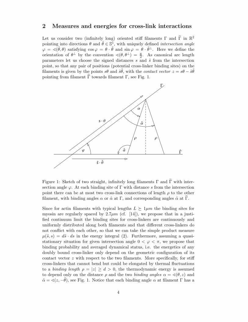
Let us consider two (infinitely long) oriented stiff filaments Γ and Γ in R2

pointing into directions θ and θ ∈ S1, with uniquely defined intersection angle

ϕ = ∢(θ, θ) satisfying cosϕ = θ · θ and sinϕ = θ · θ⊥. Here we define theorientation of θ⊥ by the convention ∢(θ, θ⊥) = π

2 . As canonical arc lengthparameters let us choose the signed distances s and s from the intersectionpoint, so that any pair of positions (potential cross-linker binding sites) on thefilaments is given by the points sθ and sθ, with the contact vector z = sθ − sθpointing from filament Γ towards filament Γ, see Fig. 1.

Γ

Γ

ρ ρ

s · θ

s · θ

ϕ

α

α

α

Figure 1: Sketch of two straight, infinitely long filaments Γ and Γ with inter-section angle ϕ. At each binding site of Γ with distance s from the intersectionpoint there can be at most two cross-link connections of length ρ to the otherfilament, with binding angles α or α at Γ, and corresponding angles α at Γ.

Since for actin filaments with typical lengths L 1µm the binding sites formyosin are regularly spaced by 2.7µm (cf. [14]), we propose that in a justi-fied continuum limit the binding sites for cross-linkers are continuously anduniformly distributed along both filaments and that different cross-linkers donot conflict with each other, so that we can take the simple product measureµ(s, s) = ds · ds in the energy integral (2). Furthermore, assuming a quasi-stationary situation for given intersection angle 0 < ϕ < π, we propose thatbinding probability and averaged dynamical status, i.e. the energetics of anydoubly bound cross-linker only depend on the geometric configuration of itscontact vector z with respect to the two filaments. More specifically, for stiffcross-linkers that cannot bend but could be elongated by thermal fluctuationsto a binding length ρ = |z| ≥ d > 0, the thermodynamic energy is assumedto depend only on the distance ρ and the two binding angles α = ∢(θ, z) andα = ∢(z,−θ), see Fig. 1. Notice that each binding angle α at filament Γ has a

4

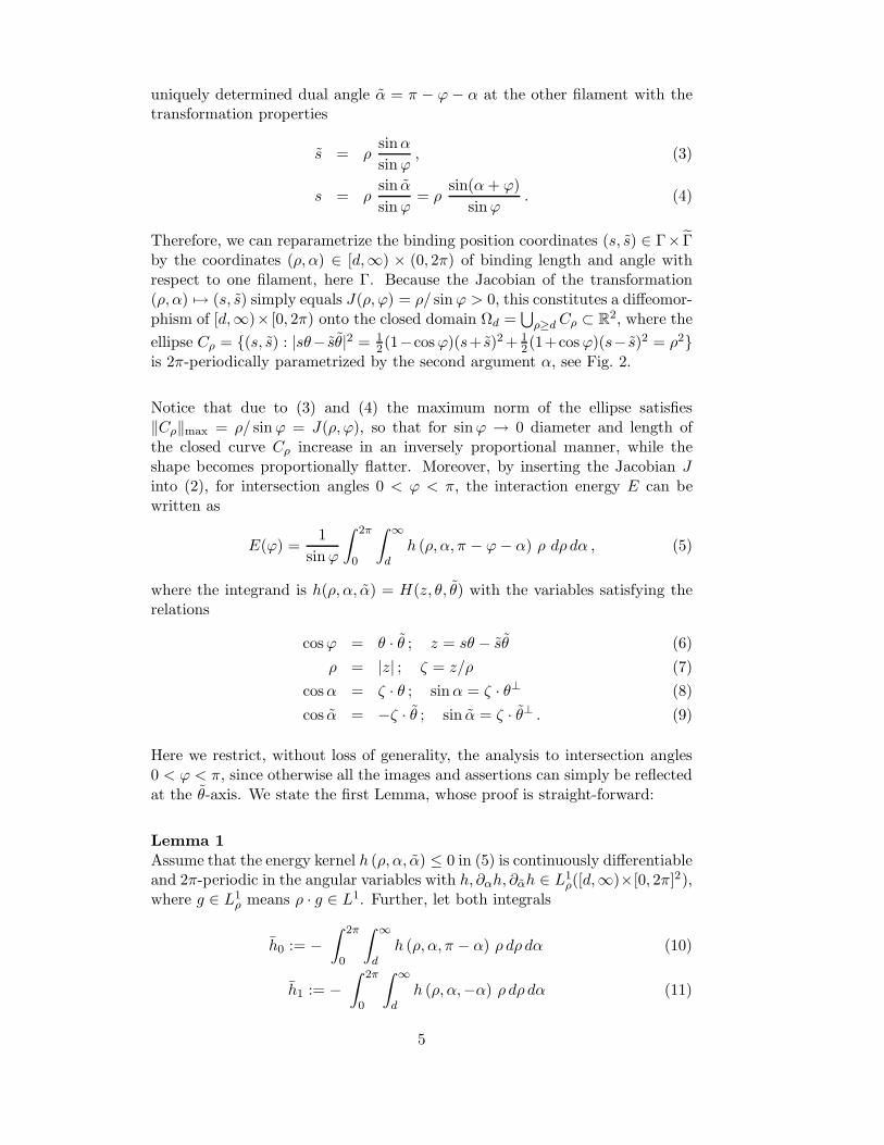
uniquely determined dual angle α = π − ϕ − α at the other filament with thetransformation properties

s = ρsinα

sinϕ, (3)

s = ρsin α

sinϕ= ρ

sin(α+ ϕ)

sinϕ. (4)

Therefore, we can reparametrize the binding position coordinates (s, s) ∈ Γ× Γby the coordinates (ρ, α) ∈ [d,∞) × (0, 2π) of binding length and angle withrespect to one filament, here Γ. Because the Jacobian of the transformation(ρ, α) 7→ (s, s) simply equals J(ρ, ϕ) = ρ/ sinϕ > 0, this constitutes a diffeomor-phism of [d,∞)× [0, 2π) onto the closed domain Ωd =

⋃ρ≥d Cρ ⊂ R

2, where the

ellipse Cρ = (s, s) : |sθ− sθ|2 = 12(1−cosϕ)(s+ s)2 + 1

2(1+cosϕ)(s− s)2 = ρ2is 2π-periodically parametrized by the second argument α, see Fig. 2.

Notice that due to (3) and (4) the maximum norm of the ellipse satisfies‖Cρ‖max = ρ/ sinϕ = J(ρ, ϕ), so that for sinϕ → 0 diameter and length ofthe closed curve Cρ increase in an inversely proportional manner, while theshape becomes proportionally flatter. Moreover, by inserting the Jacobian Jinto (2), for intersection angles 0 < ϕ < π, the interaction energy E can bewritten as

E(ϕ) =1

sinϕ

∫ 2π

0

∫ ∞

dh (ρ, α, π − ϕ− α) ρ dρ dα , (5)

where the integrand is h(ρ, α, α) = H(z, θ, θ) with the variables satisfying therelations

cosϕ = θ · θ ; z = sθ − sθ (6)

ρ = |z| ; ζ = z/ρ (7)

cosα = ζ · θ ; sinα = ζ · θ⊥ (8)

cos α = −ζ · θ ; sin α = ζ · θ⊥ . (9)

Here we restrict, without loss of generality, the analysis to intersection angles0 < ϕ < π, since otherwise all the images and assertions can simply be reflectedat the θ-axis. We state the first Lemma, whose proof is straight-forward:

Lemma 1Assume that the energy kernel h (ρ, α, α) ≤ 0 in (5) is continuously differentiableand 2π-periodic in the angular variables with h, ∂αh, ∂αh ∈ L1

ρ([d,∞)×[0, 2π]2),where g ∈ L1

ρ means ρ · g ∈ L1. Further, let both integrals

h0 := −∫ 2π

0

∫ ∞

dh (ρ, α, π − α) ρ dρ dα (10)

h1 := −∫ 2π

0

∫ ∞

dh (ρ, α,−α) ρ dρ dα (11)

5

s

s

Cd

Cρ

d < ρ

s− s+

Figure 2: Representation of possible cross-linker states in the (s, s) coordinatespace with Cρ denoting all pairs of binding sites that are connected by a cross-link of length ρ. For minimal length ρ = d the binding energy k(ρ) in (17)has a negative jump representing the repulsive function of such cross-linkers onCd, thereby serving as ‘spacers’ between the filaments. As argued in the text,the ellipses become longer and flatter (around one or the two diagonals) forsinϕ→ 0. The marked interval [s−, s+] on the s-axis denotes the binding siteson a shorter filament Γ with finite length L = s+ − s−, intersecting a muchlonger filament Γ, see section 5.

be positive. Then the energy functional E in (5) is continuously differentiableon the open interval (0, π) with the following asymptotic behavior near the twosingular boundary points ϕ∗ = 0 and π (with h = h0 or h1, respectively):

E(ϕ) = − h

sinϕ+ O (1) , (12)

dE(ϕ)

dϕ=

h cosϕ

sin2 ϕ+ O

(1

sinϕ

). (13)

Proposition 1 (Degenerate negative gradient flow)According to Lemma 1 the two intersection angles ϕ∗ = 0 and π, represent-ing parallel and anti-parallel orientation of the two filaments, respectively, are

6

locally stable steady states of the negative gradient flow described by the stan-dard differential equation with ‘relaxation rate’ λ > 0 (and with notation

ϕ(t) = dϕ(t)dt ):

ϕ = −λ · dE(ϕ)

dϕ. (14)

This differential equation degenerates at ϕ∗ = 0 and π so that the asymptoticdifference y = sinϕ = |ϕ− ϕ∗| + O(|ϕ − ϕ∗|3) fulfills

y = −λhy−2 + O(y−1) . (15)

Thus, these so-called ‘super-stable’ steady states are reached in finite positivetime t∗ such that

y(t) ∼[3λh(t∗ − t)

] 1

3 for tր t∗ . (16)

We continue by specifying physically consistent models of the interaction energykernel h in (5). While neglecting any small bending of a cross-linking polymer,which is approximately justified for myosin [14] and to a lesser degree also forα-actinin [24], we only consider thermal fluctuations of flexible binding chainsat both ends and approximately describe the cross-link by a stochastically elon-gated linear spring with Hooke spring constant η > 0, but only beyond a fixedresting length d. This reflects the assumed condition that simultaneous bindingof a cross-linker to both filaments cannot occur if the spring is under compres-sion. Since energy is consumed by binding, the resulting ‘half-spring’ energyinduced by such a doubly bound cross-linker can be written as a function ofcross-link distance ρ:

0 > − k(ρ) = − k0 · e−η2[ρ−d]2+ for ρ ≥ d , (17)

k(ρ) = 0 for ρ < d .

This energy distribution does not depend on the binding angles, it vanishes forlengths ρ < d, jumps to the minimal value −k0 at ρ = d and increases to zerowith increasing spring elongation ρ→ ∞, see Fig. 3. Then the action applied bya cross-linker onto the filaments can be expressed by the ‘variational’ incrementdk(ρ) = −k(ρ) · µf (ρ) in distributional sense, with a scalar force distributionµf given by

µf (ρ) = η[ρ− d]+ dρ − δρ=d . (18)

Whereas the first term models the attractive force by an elongated Hooke spring,the negative δ-distribution represents the repulsive action by a cross-linker atminimal length, then serving as ‘spacer’ between the filaments.

On the other hand, let us assume that the successive cross-link binding to oneand the other filament are independent of each other and do not depend on theactual spring elongation ρ, but only on the two binding angles α and α (com-pare, for example, the preferred binding of α-actinin dimers to actin filaments

7

0 0.5 1 1.5 2 2.5−3

−2.5

−2

−1.5

−1

−0.5

0

0.5

cross−link length: ρ

half−spring energy distribution

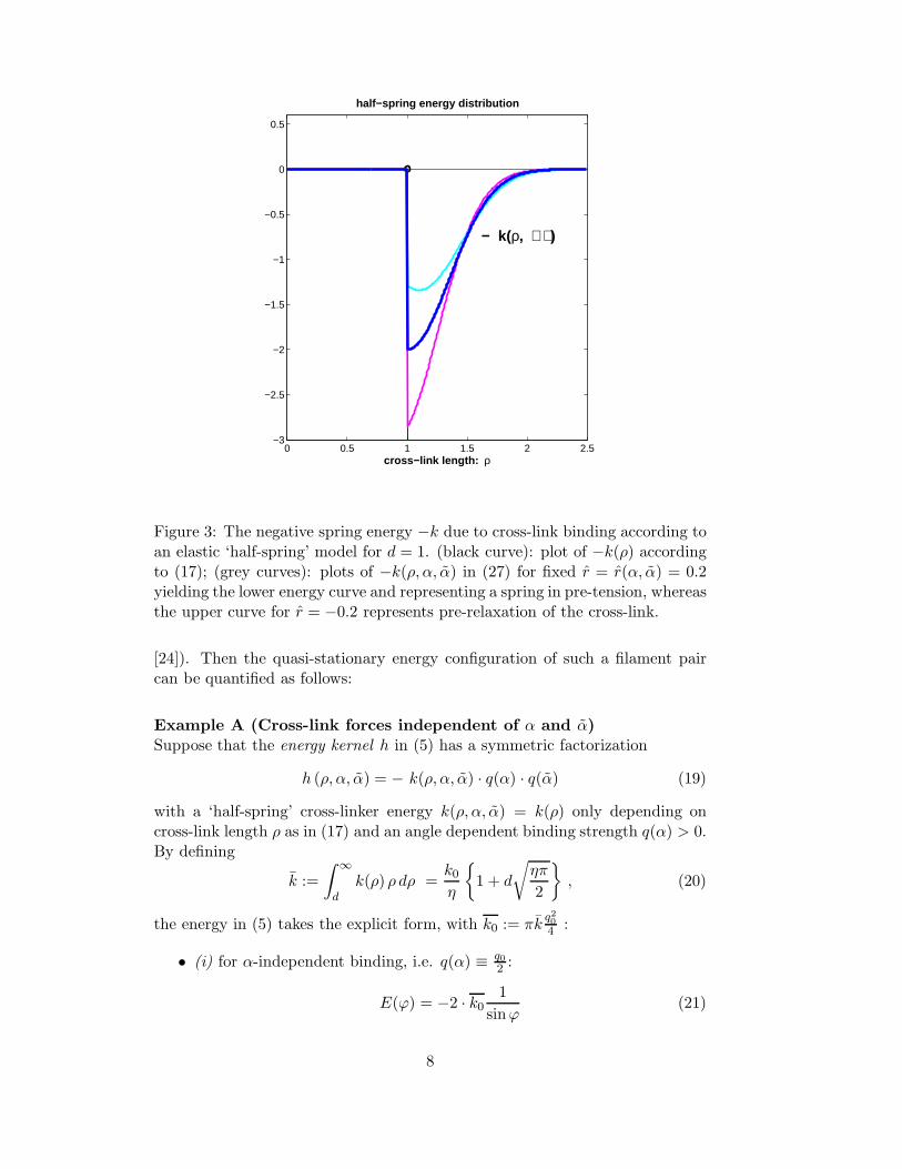
− k(ρ, ⋅ ⋅ )

Figure 3: The negative spring energy −k due to cross-link binding according toan elastic ‘half-spring’ model for d = 1. (black curve): plot of −k(ρ) accordingto (17); (grey curves): plots of −k(ρ, α, α) in (27) for fixed r = r(α, α) = 0.2yielding the lower energy curve and representing a spring in pre-tension, whereasthe upper curve for r = −0.2 represents pre-relaxation of the cross-link.

[24]). Then the quasi-stationary energy configuration of such a filament paircan be quantified as follows:

Example A (Cross-link forces independent of α and α)Suppose that the energy kernel h in (5) has a symmetric factorization

h (ρ, α, α) = − k(ρ, α, α) · q(α) · q(α) (19)

with a ‘half-spring’ cross-linker energy k(ρ, α, α) = k(ρ) only depending oncross-link length ρ as in (17) and an angle dependent binding strength q(α) > 0.By defining

k :=

∫ ∞

dk(ρ) ρ dρ =

k0

η

1 + d

√ηπ

2

, (20)

the energy in (5) takes the explicit form, with k0 := πkq20

4 :

• (i) for α-independent binding, i.e. q(α) ≡ q0

2 :

E(ϕ) = −2 · k01

sinϕ(21)

8

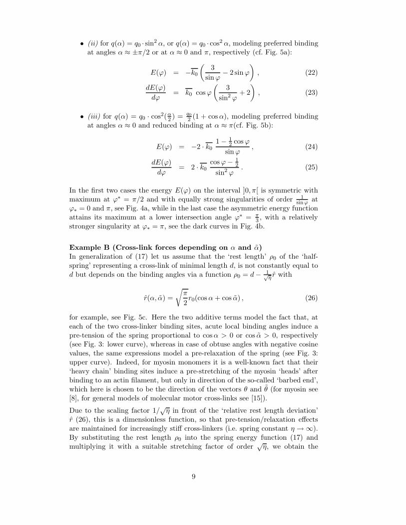
• (ii) for q(α) = q0 · sin2 α, or q(α) = q0 · cos2 α, modeling preferred bindingat angles α ≈ ±π/2 or at α ≈ 0 and π, respectively (cf. Fig. 5a):

E(ϕ) = −k0

(3

sinϕ− 2 sinϕ

), (22)

dE(ϕ)

dϕ= k0 cosϕ

(3

sin2 ϕ+ 2

), (23)

• (iii) for q(α) = q0 · cos2(α2 ) = q0

2 (1 + cosα), modeling preferred bindingat angles α ≈ 0 and reduced binding at α ≈ π(cf. Fig. 5b):

E(ϕ) = −2 · k01 − 1

2 cosϕ

sinϕ, (24)

dE(ϕ)

dϕ= 2 · k0

cosϕ− 12

sin2 ϕ. (25)

In the first two cases the energy E(ϕ) on the interval ]0, π[ is symmetric withmaximum at ϕ∗ = π/2 and with equally strong singularities of order 1

sin ϕ atϕ∗ = 0 and π, see Fig. 4a, while in the last case the asymmetric energy functionattains its maximum at a lower intersection angle ϕ∗ = π

3 , with a relativelystronger singularity at ϕ∗ = π, see the dark curves in Fig. 4b.

Example B (Cross-link forces depending on α and α)In generalization of (17) let us assume that the ‘rest length’ ρ0 of the ‘half-spring’ representing a cross-link of minimal length d, is not constantly equal tod but depends on the binding angles via a function ρ0 = d− 1√

η r with

r(α, α) =

√π

2r0(cosα+ cos α) , (26)

for example, see Fig. 5c. Here the two additive terms model the fact that, ateach of the two cross-linker binding sites, acute local binding angles induce apre-tension of the spring proportional to cosα > 0 or cos α > 0, respectively(see Fig. 3: lower curve), whereas in case of obtuse angles with negative cosinevalues, the same expressions model a pre-relaxation of the spring (see Fig. 3:upper curve). Indeed, for myosin monomers it is a well-known fact that their‘heavy chain’ binding sites induce a pre-stretching of the myosin ‘heads’ afterbinding to an actin filament, but only in direction of the so-called ‘barbed end’,which here is chosen to be the direction of the vectors θ and θ (for myosin see[8], for general models of molecular motor cross-links see [15]).

Due to the scaling factor 1/√η in front of the ‘relative rest length deviation’

r (26), this is a dimensionless function, so that pre-tension/relaxation effectsare maintained for increasingly stiff cross-linkers (i.e. spring constant η → ∞).By substituting the rest length ρ0 into the spring energy function (17) andmultiplying it with a suitable stretching factor of order

√η, we obtain the

9

0 pi/2 pi−10

−8

−6

−4

−2

0

2

4

6

8

10− lambda * dE/dphi

0 pi/2 pi−10

−8

−6

−4

−2

0

2

4

6

8

10− lambda * dE/dphi

E1 (A)E2 (A)

E3 (A)E3 (B)

(a) (b)

Figure 4: Plots of interaction energies E(ϕ) between two filaments (the negativeconcave curves) and of their negative gradient flow rates −λ ·E′(ϕ) (the mono-tone curves) according to (a) eqs. (21) in Example A(i) and (22) in ExampleA(ii); to (b) eqs. (24) in Example A(iii) and (34) in Example B(iii).

following (absolute value of the) modified energy function

kη(ρ, α, α) =√η κ e

2q

2

πr(α,α)

e−1

2(√

η[ρ−d]++r(α,α))2

for ρ ≥ d , (27)

kη(ρ, α, α) = 0 for ρ < d .

In fact, its integral k, measuring the averaged potential energy of a single cross-link, is independent of the spring constant η:

k :=

∫ ∞

dkη(ρ, •, •) dρ

= κe2

q2

πr∫ ∞

0e−

1

2(r+r)2 dr

=

√π

2κe

2q

2

πr(1 − erfc(r)) , (28)

with erfc(r) :=√

2π

∫ r0 exp(− s2

2 )ds and erfc(∞) = 1. Whereas k only depends

on the two binding angles via r = r(α, α) in (26), the total spring energy in

10

analogy to (20), namely

kη =

∫ ∞

dkη(ρ, •, •) ρ dρ

=

(d− r√

η

)k +

κ√ηe− 1

2r2+2

q2

πr, (29)

also depends on η, but converges towards d · k for η → ∞. Thus, with theanalogous definition of the kernel h = hη (19), the total energy functional (5)for a filament pair can in general be computed as

Eη(ϕ) = − 1

sinϕ

∫ 2π

0kη(α, π − ϕ− α) · q(α) · q(π − ϕ− α) dα . (30)

However, in the limit η → ∞ of infinitely stiff cross-linkers, the original energydistribution kη(ρ, •, •) ρ dρ converges to the Dirac measure d · k δρ=d, so thatthe energy functional E(ϕ) = E∞(ϕ) can be represented as a global integral(2) with the singular kernel

H(z, θ, θ)µd(s, s) = −d · k(α, α) · q(α) · q(α) dα δρ=d . (31)

Here µd(s, s) describes the 1-dimensional Hausdorff measure on the quasi-ellipticcurve Cd = ρ = |z(s, s)| = d in the original (s, s)-coordinates according to(3)–(4), see also Fig. 2.

In general, calculation of E(ϕ) as an explicit function of the intersection angleϕ in closed form is not possible, however, by approximating the error-functionerfc in (28) for small values of the pre-tension strength r0 in (26), we obtain

e2

q2

πr(1 − erfc(r)) = (1+2

√2π r+O(r2))(1−

√2π r+O(r2)) = 1+

√2π r+O(r2)

and thus the simple approximative kernel representation

k(α, α) =

√π

2κ

(1 + r0(cosα+ cos α) + O(r20)

). (32)

Finally, under this assumption we derive the following explicit energy formulas,which we restrict to the two cases (i) and (iii) defined in Example A:

• (i) for α-independent binding, i.e. q(α) ≡ q0

2 :

E(ϕ) = −2 · κ0d

sinϕ, (33)

with κ0 :=(

π2

) 3

2 κq20

2 , the same standard formula as in (21), and

• (iii) for q(α) = q0

2 (1 + cosα), modeling preferred binding at angles α ≈ 0and reduced binding at α ≈ π:

E(ϕ) = −2 · κ0d

sinϕ

1 − 1

2cosϕ+ r0(1 − cosϕ)

, (34)

dE(ϕ)

dϕ= 2 · κ0 d

(1 + r0) cosϕ− (12 + r0)

sin2 ϕ. (35)

11

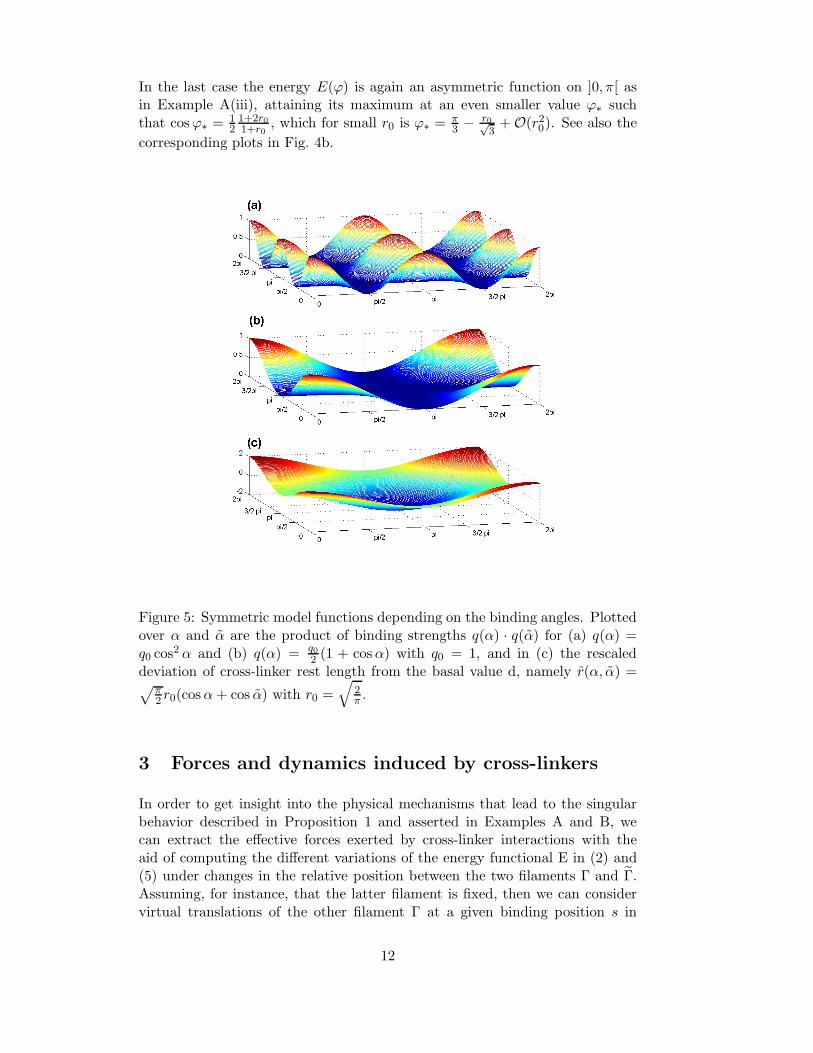
In the last case the energy E(ϕ) is again an asymmetric function on ]0, π[ asin Example A(iii), attaining its maximum at an even smaller value ϕ∗ suchthat cosϕ∗ = 1

21+2r0

1+r0, which for small r0 is ϕ∗ = π

3 − r0√3

+ O(r20). See also the

corresponding plots in Fig. 4b.

Figure 5: Symmetric model functions depending on the binding angles. Plottedover α and α are the product of binding strengths q(α) · q(α) for (a) q(α) =q0 cos2 α and (b) q(α) = q0

2 (1 + cosα) with q0 = 1, and in (c) the rescaleddeviation of cross-linker rest length from the basal value d, namely r(α, α) =√

π2 r0(cosα+ cos α) with r0 =

√2π .

3 Forces and dynamics induced by cross-linkers

In order to get insight into the physical mechanisms that lead to the singularbehavior described in Proposition 1 and asserted in Examples A and B, wecan extract the effective forces exerted by cross-linker interactions with theaid of computing the different variations of the energy functional E in (2) and(5) under changes in the relative position between the two filaments Γ and Γ.Assuming, for instance, that the latter filament is fixed, then we can considervirtual translations of the other filament Γ at a given binding position s in

12

two orthogonal directions ζ and ζ⊥, i.e. in direction of the cross-linker contactvector z = ρ · ζ, see (6)–(7), and orthogonal to it. The first variation (δζ)means that the cross-linker length ρ is increased, say by dρ, while both bindingangles α and α stay fixed. The other variation (δζ⊥) induces a rotation of thecross-linker around the fixed binding site s on Γ such that the local turn, sayby dσ, of the lever (with constant length ρ) induces changes of both bindingangles α and α by dα = −dα = 1/ρ dσ, since the sum α+ α = π−ϕ stays fixeddue to pure translation of the whole filament Γ under constant ϕ. Thus, theforce resulting from virtual spring length variations (δζ) is the contracting orspacing spring force, which in terms of the kernel h (19) can be written as

Kf (s, s) = − ∂ρh(ρ, α, α) · ζ = ∂ρk(ρ, α, α) · q(α) · q(α) · ζ , (36)

where the ‘unit cross-link vector’ is ζ = ζθ(α) = (cosα)θ+(sinα)θ⊥, cf. (7)–(9).On the other hand, from rotational variations (δζ⊥) we obtain the sum of twocross-link torque forces

Kω(s, s) = −1

ρ∂αh(ρ, α, α) · ζ⊥ , (37)

Kω(s, s) =1

ρ∂αh(ρ, α, α) · ζ⊥ , (38)

so that the total force exerted by a cross-linker connection from the fixed bindingsite s at Γ to the binding site s on Γ is given by the following force kernelK : Γ × Γ → R

2:K = Kf +Kω +Kω . (39)

Remark (Integral representation of total forces)First, let us mention that integration over the local spring force in (36) yields,using integration by parts over ρ, an explicit expression for the total force dueto contractile/spacing action of cross-linkers in terms of the integral kernel h:

Kf :=

∫

Γ

∫

eΓKf (s, s) ds ds = − 1

sinϕ

∫ 2π

0

∫ ∞

0∂ρh(ρ, α, α) · ζ ρdρ dα

=1

sinϕ

∫ 2π

0

∫ ∞

0h(ρ, α, α) · ζ dρ dα , (40)

where this identity also holds for Example B, even in the limiting case of in-finite stiffness (η → ∞) for the kernel in (31). Then, introducing the nota-tion hϕ(ρ, α) = h(ρ, α, π − ϕ − α) and noticing ∂αhϕ = ∂αh − ∂αh as well asζ(α) = −∂αζ

⊥(α), we conclude that the total force onto Γ vanishes:

K =

∫

Γ

∫

eΓK(s, s) ds ds

=1

sinϕ

∫ 2π

0

∫ ∞

d

h · ζ − ∂αhϕ · ζ⊥

dρ dα

= − 1

sinϕ

∫ ∞

d

∫ 2π

0∂α(hϕ · ζ⊥) dα dρ = 0 .

13

This assertion has to be true since the defining energy E(ϕ) does only dependon ϕ and is therefore invariant under pure translations of one filament withrespect to the other. Thus, the only global dynamic action on the filamentpair is the total torque Ω = − δE

δϕ = −E′(ϕ) to be computed by variation of Ewith respect to the intersection angle ϕ itself, while holding s and s fixed. Thiscan be computed and identified with the integral formula obtained by usingthe local forces in (36)–(38) and the mechanical lever laws for torque moments,with virtual rotation around the fixed intersection point (s = s = 0), yieldingthe following equality

Ω =

∫

Γ

∫

eΓ

sθ⊥ · (σKf +Kω) + sθ⊥ · ((1 − σ)Kf +Kω)

ds ds . (41)

Here σ is an arbitrary fraction of unity, e.g. σ = 1/2, because one observes thesymmetric identity

sθ⊥ · ζ = sθ⊥ · ζ =ρ

sinϕsinα · sin α . (42)

Thus, the resulting differential equation for temporal changes in ϕ (see Prop.3 below) is the negative gradient flow (14). However, the local forces appear-ing in the two kernels Kω and Kω arise from variations (δζ⊥) that change thebinding angles, so that in the presented energy model they can be associatedto resisting ‘torque’ forces of cross-linkers that stay bounded to actin filamentsduring the variation of binding angles. Such a model (satisfying the gradientflow kinetics) could be relevant for physical situations of steadily cross-linkedmolecules, whereas for the biophysical situation of ongoing dissociation and re-association of cross-linking dimers (as myosin or filamin) on a mesoscale (ofseveral seconds) during slow filament motion on a macroscale (of minutes), wehave to modify the model. Since for computing the virtual forces, only varia-tions on an even faster microscale (fractions of seconds) are considered, we canassume that during this short time the cross-links stay bounded. Then due tothe model interpretation of the binding strengths, q(α) and q(α), these wouldnot change, and the only remaining variations are that of the spring energyk(ρ, α, α). Moreover, if we suppose that the angle-dependence of k (for themodel in Example B) via the pre-tension/relaxation function r has been real-ized already during binding of the cross-link, then the only effective variationthat remains is the one in cross-linker length (δζ). Thus, as local force vectorkernel we can take K = Kf and assume Kω = Kω = 0. Splitting K into itscomponents parallel and orthogonal to the filament Γ, namely K = K‖θ+K⊥θ⊥

and using the relations (8)–(9) as well as (42), we obtain the following explicitformulas for the total torque and parallel and orthogonal force components ex-pressed in (ρ, α, α)-coordinates:

Proposition 2 (Total torque and forces onto one filament)Assume that bound cross-links only apply forces to the filaments due to elon-gation of their ‘half-spring’ but not due to bending or tilting of their binding

14

angles, thus Kω = Kω = 0. Then under the assumption that filament Γ isfixed, local variation of cross-linkers leads to the force kernel K = Kf in (36)yielding the following global torque Ω and the parallel and orthogonal forcesF ‖ =

∫Γ

∫eΓK‖(s, s) ds ds and F⊥ =

∫Γ

∫eΓK⊥(s, s) ds ds onto filament Γ (again

using integration by parts):

Ω = − 1

sin2 ϕ

∫ 2π

0

∫ ∞

d∂ρh(ρ, α, α) ρ2dρ sinα sin α dα

=2

sin2 ϕ

∫ 2π

0

∫ ∞

dh(ρ, α, α) ρ dρ sinα sin α dα (43)

F ‖ =1

sinϕ

∫ 2π

0

∫ ∞

dh(ρ, α, α) dρ cosα dα (44)

F⊥ =1

sinϕ

∫ 2π

0

∫ ∞

dh(ρ, α, α) dρ sinα dα (45)

with the total translational force given by

K = Kf = F ‖ θ + F⊥θ⊥ . (46)

Before computing explicit expressions for Ω, F ‖ and F⊥ as functions of ϕ inspecific examples, let us write down the dynamical equations describing theresulting motion of one filament with respect to the other.

Proposition 3 (Over-damped dynamics of filament motion)Let us assume that one filament, say Γ, is held fixed and represented by theoriented x-axis, for instance. Then the dynamics of the other filament, Γ, underover-damping conditions (i.e. strong friction relative to inertia) is determinedby the following force balance equations for the three independent types ofmotion (rotation, parallel and orthogonal translation), where each of them caneventually have a different friction coefficient (λ−1):

dϕ

dt= λ Ω , (47)

ds

dt= λ‖ F

‖ , (48)

ds⊥

dt= λ⊥ F⊥ , (49)

with the torque Ω the other forces defined in (43)–(45). Let us remark that forfinite filaments the inverse friction coefficients λ due to Stokes formula woulddepend on its length L in a manner that λ⊥ = 2 · λ‖ ∼ L−1, but λ ∼ L−2,compare section 5.In general, the motion of Γ is completely determined by the intersection coor-dinate x = R(t) with filament Γ (the x-axis), the intersection angle ϕ = Φ(t)and the signed segment length s = S(t) between the intersection point (R(t), 0)and a freely chosen but fixed point (X(t), Y (t)) on filament Γ, e.g. the filamentmass center, see Fig. 7d below. Thus we obtain the representation

X = R+ S cos Φ , Y = S sin Φ , (50)

15

where the defining time-dependent variables Φ, S, R satisfy the system of differ-ential equations (again for angles 0 < Φ < π, without restriction of generality):

dΦ

dt= λ Ω(Φ) , (51)

dS

dt= λ‖ F

‖(Φ) +λ⊥

tan ΦF⊥(Φ) , (52)

dR

dt= − λ⊥

sin ΦF⊥(Φ) . (53)

The last equation (53) and the second term in equation (52) arise from orthogo-nal shifts of filament Γ. Thus, for infinitely long filaments the ‘leading’ degener-ate ODE (51) autonomously determines the dynamics of filament intersectionangle Φ(t), whereas subsequent integration of the other two, Φ(t)-dependentequations (52)–(53) yields the relative position of one filament with respect tothe other. For filaments of finite length, the analogous ODE system turns outto be nonlinearly coupled in the first two variables, see section 5.

In order to characterize and visualize different types of filament dynamics forthe various interaction models, we now compute the torque Ω(ϕ) as well as theforce terms F ‖(ϕ) and F⊥(ϕ) for the examples introduced in section 2:

Example A (Cross-link forces only depending on ρ)With the conditions and definitions after eq. (20) we can state:

• (i) and (ii) Since in these cases the force kernel h(ρ, α, π −ϕ−α) in (40)turns out to be an odd function of the periodic variable α, both integratedforces F ‖ and F⊥ vanish. Thus, for these models with symmetric interac-tion energy E(ϕ) = E(π−ϕ) the filament dynamics shows no translations,only rotation around the fixed intersection point. In the standard case(i) we obtain the torque Ω = −E′(ϕ) for the energy in (21) and, thus, aresulting negative gradient flow. On the contrary, this does not hold for(ii), where in case of q(α) = q0 sin2 α we have

Ω(ϕ) = −k0 cosϕ

5

sin2 ϕ− 2

, (54)

and for q(α) = q0 cos2 α

Ω(ϕ) = −k0 cosϕ

1

sin2 ϕ− 2

. (55)

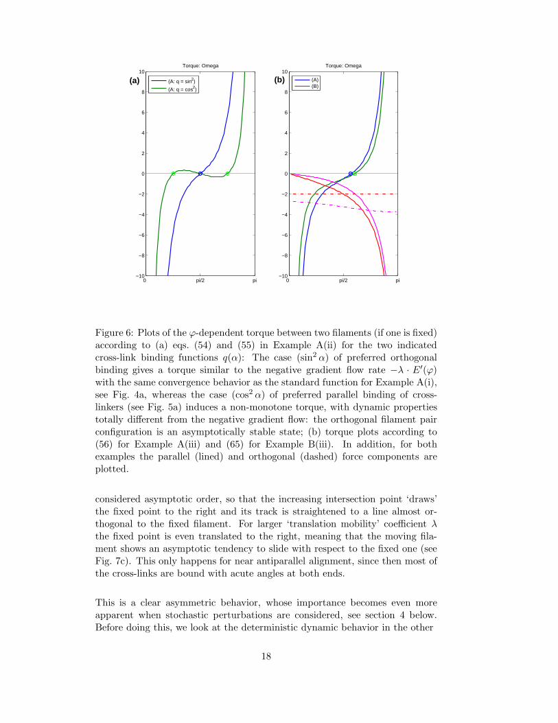
Whereas in the first case the symmetric function Ω(ϕ) is monotone in-creasing with the unstable zero ϕ∗ = π/2, in the second case this or-thogonal configuration is a stable equilibrium state with two additionalunstable zeros at ϕ∗ = π/2 ± π/4, see the plots in Fig. 6a.

16

• (iii) With the asymmetric binding strength q(α) = q0

2 (1 + cosα) also thetorque function becomes asymmetric according to (43):

Ω(ϕ) = −k0

2 cosϕ− 1

2

sin2 ϕ+ 1

, (56)

while the global forces according to (44) and (45) are

F ‖(ϕ) = −2kη1 − cosϕ

sinϕ, (57)

F⊥(ϕ) = −2kη , (58)

with kη =(

π2

) 3

2 k0√η

q20

4 . Notice that the total orthogonal force onto the

filament in (58) is just a negative constant (for 0 < ϕ < π)!

Only for the last Example A(iii) the intersection point (R, 0) between the mov-ing filament and the fixed one changes due to parallel and orthogonal net forces,see Fig. 6b. Since there is a constant orthogonal ‘right-shift’ of the filament (tothe right side with respect to its orientation vector θ) but a simultaneous par-allel ‘back-draw’, at least for angles Φ > 0, one cannot easily conclude, inwhich direction the filament is translocated. Therefore, we have to study theODE-System (51)–(53), which for parameter values k0 = 2kη = 1 (equivalent

to d +√

2πη = 1) and inverse frictions λ = 1, λ‖ = λ and λ⊥ = 2 · λ (all

parameters and variables in dimensionless units) yields

dΦ

dt= −

2 cos Φ − 1

2

sin2 Φ+ 1

, (59)

dS

dt= −λ1 + cos Φ

sin Φ, (60)

dR

dt= 2 · λ 1

sin Φ. (61)

According to Fig. 6b the intersection angle Φ(t) generically converges to one ofthe two alignment states, where with (15)–(16) we obtain the following asymp-totic behavior:At parallel alignment, see Fig. 7b, we have the rapid convergence Φ(t) ∼[t∗ − t]

1/3+ in finite time, so that by R(t) ∼ 2λ

Φ(t) ∼ −S(t) we obtain the cor-

responding convergence R∗ −R(t) ∼ [t∗ − t]2/3+ ∼ Φ(t)2. Thus, the intersection

point R(t) increases a bit, but gets stationary at a certain value R∗ even morerapidly than the intersection angle. Since on this asymptotic order the sum(R+ S)(t) ∼ R∗ + S∗ is already stationary, the fixed point (marked in Fig. 7d)on the moving filament does perform an almost circular arc while approachingthe fixed filament.At antiparallel alignment, see Fig. 7a, we get the same asymptotic behavior for

Φ(t) = π − Φ(t) and R(t), even with a bit stronger coefficient, but now thesegment length S(t) ∼ S∗ on the moving filament is already stationary on the

17

0 pi/2 pi−10

−8

−6

−4

−2

0

2

4

6

8

10Torque: Omega

0 pi/2 pi−10

−8

−6

−4

−2

0

2

4

6

8

10Torque: Omega

(A: q = sin2)

(A: q = cos2)

(A)(B)

(a) (b)

Figure 6: Plots of the ϕ-dependent torque between two filaments (if one is fixed)according to (a) eqs. (54) and (55) in Example A(ii) for the two indicatedcross-link binding functions q(α): The case (sin2 α) of preferred orthogonalbinding gives a torque similar to the negative gradient flow rate −λ · E′(ϕ)with the same convergence behavior as the standard function for Example A(i),see Fig. 4a, whereas the case (cos2 α) of preferred parallel binding of cross-linkers (see Fig. 5a) induces a non-monotone torque, with dynamic propertiestotally different from the negative gradient flow: the orthogonal filament pairconfiguration is an asymptotically stable state; (b) torque plots according to(56) for Example A(iii) and (65) for Example B(iii). In addition, for bothexamples the parallel (lined) and orthogonal (dashed) force components areplotted.

considered asymptotic order, so that the increasing intersection point ‘draws’the fixed point to the right and its track is straightened to a line almost or-thogonal to the fixed filament. For larger ‘translation mobility’ coefficient λthe fixed point is even translated to the right, meaning that the moving fila-ment shows an asymptotic tendency to slide with respect to the fixed one (seeFig. 7c). This only happens for near antiparallel alignment, since then most ofthe cross-links are bound with acute angles at both ends.

This is a clear asymmetric behavior, whose importance becomes even moreapparent when stochastic perturbations are considered, see section 4 below.Before doing this, we look at the deterministic dynamic behavior in the other

18

−10 −8 −6 −4 −2 0 2−5

−4

−3

−2

−1

0

1

2

3

4

5

(a)

−4 −2 0 2 4 6 8 10−5

−4

−3

−2

−1

0

1

2

3

4

5

(b)

−8 −6 −4 −2 0 2 4−5

−4

−3

−2

−1

0

1

2

3

4

(c)

−4 −2 0 2 4 6 8 10−5

−4

−3

−2

−1

0

1

2

3

4

5

(d)

(X,Y)

SR

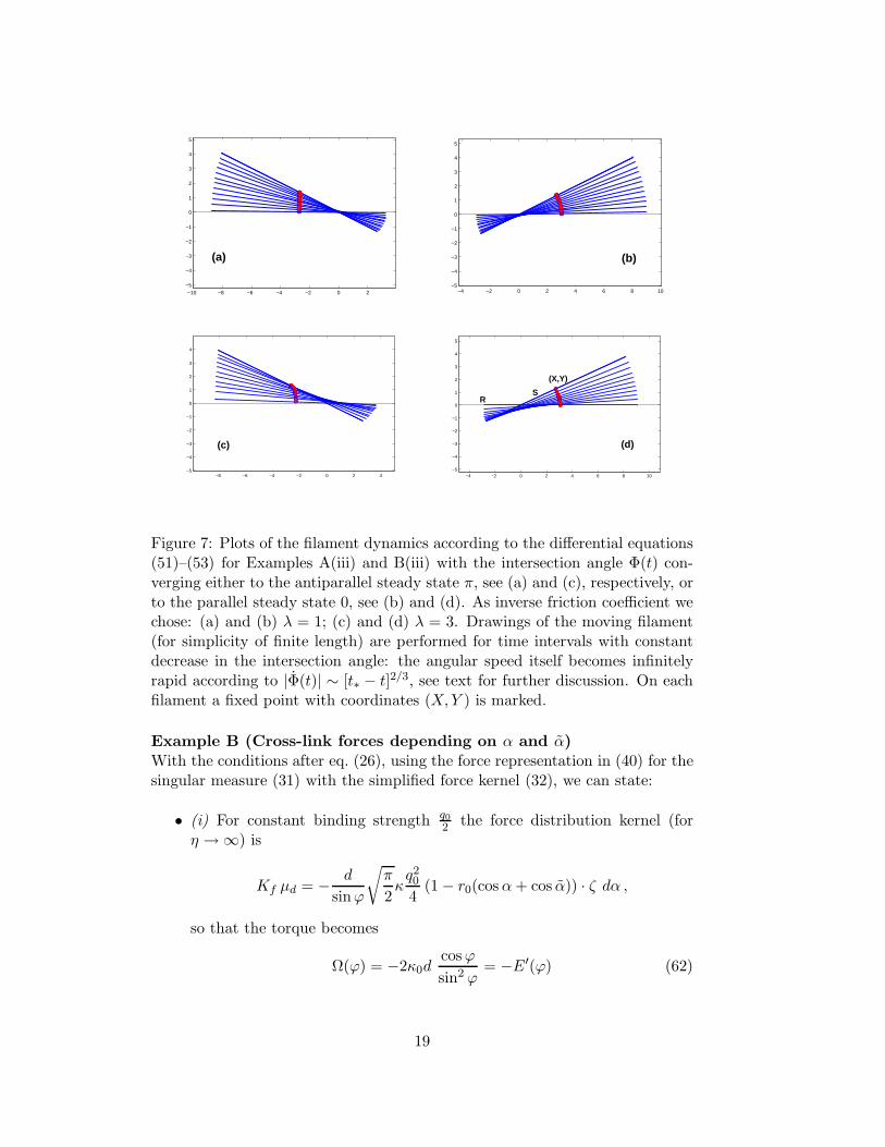
Figure 7: Plots of the filament dynamics according to the differential equations(51)–(53) for Examples A(iii) and B(iii) with the intersection angle Φ(t) con-verging either to the antiparallel steady state π, see (a) and (c), respectively, orto the parallel steady state 0, see (b) and (d). As inverse friction coefficient wechose: (a) and (b) λ = 1; (c) and (d) λ = 3. Drawings of the moving filament(for simplicity of finite length) are performed for time intervals with constantdecrease in the intersection angle: the angular speed itself becomes infinitelyrapid according to |Φ(t)| ∼ [t∗ − t]2/3, see text for further discussion. On eachfilament a fixed point with coordinates (X,Y ) is marked.

Example B (Cross-link forces depending on α and α)With the conditions after eq. (26), using the force representation in (40) for thesingular measure (31) with the simplified force kernel (32), we can state:

• (i) For constant binding strength q0

2 the force distribution kernel (forη → ∞) is

Kf µd = − d

sinϕ

√π

2κq204

(1 − r0(cosα+ cos α)) · ζ dα ,

so that the torque becomes

Ω(ϕ) = −2κ0dcosϕ

sin2 ϕ= −E′(ϕ) (62)

19

and the two force components

F ‖(ϕ) = −κ0 r01 − cosϕ

sinϕ(63)

F⊥(ϕ) = −κ0 r0 . (64)

Notice that these forces have exactly the same structure as in ExampleA(iii) above, but with a symmetric torque function as in the standardcase A(i).

• (iii) For asymmetric binding as in Example A(iii) but with angle depen-dent force we analogously obtain

Ω(ϕ) = −κ0

2d

(4 + r0(1 − cosϕ)2) · cosϕ− 1

sin2 ϕ+ 2(1 + r0) + r0 cosϕ

(65)and

F ‖(ϕ) = − κ0

sinϕ

(1 + r0 −

3

4r0 cosϕ)(1 − cosϕ) +

r04

sin2 ϕ

(66)

F⊥(ϕ) = −κ0

1 +

5

4r0 −

r02

cosϕ

. (67)

One can show that both force functions F ‖ and F⊥ are negative andmonotone decreasing in the variable ϕ, see Fig. 6b.

According to the plots in Fig. 6b this last Example B(iii) modeling myosin actionbetween the two filaments, shows qualitatively the same behavior as the Exam-ple A(iii) with the same cross-linker binding strength function, namely preferredpolar binding in direction of the oriented filaments. Indeed, the asymptotic co-efficients are a bit larger and produce an even more rapid convergence duringantiparallel alignment and a stronger sliding effect near antiparallel alignment(see Fig. 7). Thus, the additional assumption of angle-dependent cross-linkerforce in (27) for Examples B strengthens the asymmetric convergence behav-ior, which obviously is induced already by the assumed asymmetric cross-linkerbinding. Again, with additional stochastic noise introduced in the followingsection, these effects will become more prominent.

4 Stochastic dynamics

So far the dynamic action of the cross-links was modeled in a mean field ap-proximation, where with an assumed constant reservoir of cross-linking dimersin solution the energy integral kernel hϕ(ρ, α) = ρ

sinϕh(ρ, α, α) according to (5)measured the mean expected density distribution of bound cross-linkers withrespect to their length (ρ) and binding angle (α). Moreover, according to (36)the density of mean force locally exerted by cross-linkers onto one filament could

20

be expressed by the kernel Kϕ(ρ, α) = − ρsinϕ∂ρh(ρ, α, α) · ζ(α). Regarding that

molecular association and dissociation of cross-linkers are Poisson processes,then also the expected variance will be locally distributed as proportional tohϕ. Thus, for any given intersection angle ϕ there is a constant bf measuring thenoise amplitude (depending on temperature), so that per infinitesimally smalltime step dt the local impulse increment density induced by cross-linkers, usuallygiven by dtP = Kϕ dt, can now be written as a sum dtP = Kdet

ϕ dt+Kstochϕ dWt

with a deterministic increment dt and a stochastic Wiener increment dWt:

dtP (s, s) ds ds =

(−∂ρh

ρ

sinϕdt+ bf

√h

ρ

sinϕdWt

)dρ dα · ζ . (68)

Then, computing the total impulse increment dtP = Kdet dt + Kstoch dWt ac-cording to the first integral representation in (40) we obtain stochastic integralsfor each of the two force components of K = F ‖θ + F⊥θ⊥ with the followingproperties:

Proposition 4 (Stochastic differential equations for filament motion)In the situation of Proposition 3, with stochastic noise introduced as describedabove, instead of (47)–(49) we obtain a system of degenerate stochastic differ-ential equations (for any 2π-periodic ϕ)

dϕ = λ

(sign(sinϕ)Ωdet(ϕ) dt + b(ϕ)| sinϕ|− 3

2 dWt

), (69)

ds = λ‖(F

‖det(ϕ) dt + b‖(ϕ)| sinϕ|− 1

2 dWt

), (70)

ds⊥ = λ⊥(sign(sinϕ)F⊥

det(ϕ) dt + b⊥(ϕ)| sinϕ|− 1

2 dWt

). (71)

Here the deterministic parts of torque and translation forces are given by theintegrals defined in (43)–(45), or by the computed formulas in Examples A andB of section 3 (as they are given for positive ϕ only). Moreover, the relative noisecoefficients b#(ϕ) depend continuously on cosϕ and sinϕ, satisfying analogousintegral representations for the variances of the stochastic torque and forcecomponents

b2 = | sinϕ|3 Var(Ωstoch) = b2f

∫ 2π

0

∫ ∞

d|h(ρ, α, α)|ρ3dρ (sinα sin α)2dα(72)

b2‖ = | sinϕ|Var(F‖stoch) = b2f

∫ 2π

0

∫ ∞

d|h(ρ, α, α)| ρdρ cos2 αdα (73)

b2⊥ = | sinϕ|Var(F⊥stoch) = b2f

∫ 2π

0

∫ ∞

d|h(ρ, α, α)| ρdρ sin2 αdα . (74)

Since the deterministic non-linearities degenerate like Ωdet ∼ | sinϕ|−2 and

F#det ∼ | sinϕ|−1, the stochastic increments in eqs. (69)–(71) degenerate at a

lower order. In particular, using the same notation as for the asymptotic deter-ministic equation (15), near the singularities ϕ∗ = 0 and π the leading stochasticequation (69) can asymptotically be written as

dy = −a · |y|−m dt+ b · |y|γ−m dWt (75)

21

with m = 2 and γ = 12 . This class of degenerate SDEs does not always lead to

well defined stationary processes:

0 0.5 1 1.5 2 2.5 3 3.5 4 4.5 5−1.5

−1

−0.5

0

0.5

1

1.5

(a)

0 200 400 600 800 1000−1.5

−1

−0.5

0

0.5

1

1.5

(b)

Figure 8: Properties of the asymptotic process yt for the stochastic variablesin Φt satisfying (75) with γ = 1

2 and m = 2. (a) Stochastic path (black)together with the path of the transformed variable zt = y3

t (grey), usu-ally of lower absolute value; (b) empirical distribution of the yt values (his-togram) and theoretical probability distribution according to (76): p(y) =2ν

√ν/π y2 exp(−ν y2) with ν = a/b2, here a = 1 and b = 0.3.

Lemma 2 (Resolving power law singularities in SDEs)The degenerate SDE in (75) with m > 0 describes a nontrivial generalizedGauss process that is asymptotically stationary only if the exponents satisfythe condition 0 < γ < m+1

2 . The stationary process has the symmetric bimodalprobability distribution

p(y) dy = pm · |y|me−2a

µb2|y|µ

dy (76)

with µ = m+ 1− 2γ > 0 and a positive scaling factor pm, see Fig. 8b. Realiza-tions of the stationary process randomly switch between positive and negativevalues, with super-exponentially long switching intervals (‘resting times’) andintermittent phases of very fast oscillations, see Fig. 8a.

Proof: Consider the transformed stochastic variable z = sign(y)|y|m+1 satis-fying the following non-continuous SDE, with a right-hand side that performsa negative jump at zero, a so-called ‘negative sign-type’ SDE:

dz = −(m+ 1)a · sign(z) dt + (m+ 1)b · |z|β dWt (77)

with β = γm+1 > 0. Computation of the Kolmogorov forward equation re-

veals that (77) possesses stationary solutions only if β < 1/2, with sym-metric unimodal stationary distribution p(z) ∼ exp(−ν|z|1−2β), where ν =a/

((m+ 1)(1

2 − β)b2). While the deterministic solution without noise consists

of straight lines reaching the absorbing state zero in finite time, the stochasticrealizations show weighted random increments with sufficiently strong pertur-bations of amplitude |z|β > √

z, which are able to drive the solution away from

22

zero, fast enough to overcome the deterministic absorption.

Applying the results of Lemma 2 to the original asymptotic differential equa-tion (75) for the stochastic variable yt = sin Φt, satisfying the condition 0 <γ = 1

2 <32 = m+1

2 for m = 2, we conclude that the stochastic perturbations of

order | sinϕ|− 3

2 in (69) are not too strong, but strong enough to overcome theinfinitely fast ‘attraction’ to zero by the deterministic term dϕ/dt ∼ | sinϕ|−2

and to induce a bimodal stationary distribution, see the stochastic realizationin Fig. 8. Interpreted in terms of the biophysical model, this asymptotic re-sult says that the more cross-linkers are active to attract the two filamentstowards alignment, with infinitely increasing speed for sinΦt → 0, the morefluctuations of the stochastic binding process occur and disturb the attraction,strongly enough to prevent complete alignment. Instead, the intersection anglebetween the two filaments steadily fluctuates around zero, not in a Gaussianmanner as for regularly stable steady states, but with a generalized biomodalGauss distribution so that too small angles are avoided.

0 pi/2 pi

0

pi/2

pi

regularizing angular transformation

phi

ψ

Λ

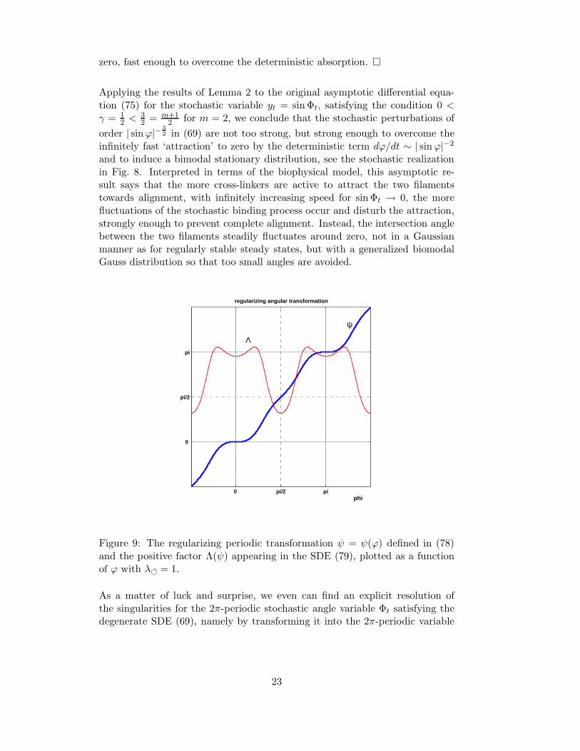
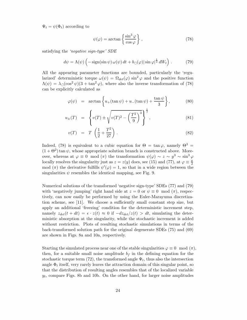
Figure 9: The regularizing periodic transformation ψ = ψ(ϕ) defined in (78)and the positive factor Λ(ψ) appearing in the SDE (79), plotted as a functionof ϕ with λ = 1.

As a matter of luck and surprise, we even can find an explicit resolution ofthe singularities for the 2π-periodic stochastic angle variable Φt satisfying thedegenerate SDE (69), namely by transforming it into the 2π-periodic variable

23

Ψt = ψ(Φt) according to

ψ(ϕ) = arctan

sin3 ϕ

cosϕ

, (78)

satisfying the ‘negative sign-type’ SDE

dψ = Λ(ψ)(− sign(sinψ)ω(ψ) dt + b(ϕ)| sinϕ| 12 dWt

). (79)

All the appearing parameter functions are bounded, particularly the ‘regu-larized’ deterministic torque ω(ψ) = Ωdet(ϕ) sin2 ϕ and the positive functionΛ(ψ) = λ(cos2 ψ)(3 + tan2 ϕ), where also the inverse transformation of (78)can be explicitly calculated as

ϕ(ψ) = arctan

u+(tanψ) + u−(tanψ) +

tanψ

3

, (80)

u±(T ) =

v(T ) ±

√

v(T )2 −(T 2

9

)3

1

3

, (81)

v(T ) = T

(1

2+T 2

27

). (82)

Indeed, (78) is equivalent to a cubic equation for Θ = tanϕ, namely Θ3 =(1 + Θ2) tanψ, whose appropriate solution branch is constructed above. More-over, whereas at ϕ ≡ 0 mod (π) the transformation ψ(ϕ) ∼ z ∼ y3 ∼ sin3 ϕlocally resolves the singularity just as z = z(y) does, see (15) and (77), at ϕ ≡ π

2mod (π) the derivative fulfills ψ′(ϕ) = 1, so that in a wide region between thesingularities ψ resembles the identical mapping, see Fig. 9.

Numerical solutions of the transformed ‘negative sign-type’ SDEs (77) and (79)with ‘negatively jumping’ right hand side at z = 0 or ψ ≡ 0 mod (π), respec-tively, can now easily be performed by using the Euler-Marayuma discretiza-tion scheme, see [11]. We choose a sufficiently small constant step size, butapply an additional ‘freezing’ condition for the deterministic increment step,namely zdet(t + dt) = ǫ · z(t) ≈ 0 if −dzdet/z(t) > dt, simulating the deter-ministic absorption at the singularity, while the stochastic increment is addedwithout restriction. Plots of resulting stochastic simulations in terms of theback-transformed solution path for the original degenerate SDEs (75) and (69)are shown in Figs. 8a and 10a, respectively.

Starting the simulated process near one of the stable singularities ϕ ≡ 0 mod (π),then, for a suitable small noise amplitude bf in the defining equation for thestochastic torque term (72), the transformed angle Ψt, thus also the intersectionangle Φt itself, very rarely leaves the attraction domain of this singular point, sothat the distribution of resulting angles resembles that of the localized variableyt, compare Figs. 8b and 10b. On the other hand, for larger noise amplitudes

24

0.06 0.065 0.07 0.075 0.08 0.085 0.09 0.0952.95

3

3.05

3.1

3.15

3.2

3.25

3.3

3.35

(a)

0 50 100 150 200 250

2.95

3

3.05

3.1

3.15

3.2

3.25

3.3 (b)

0 0.01 0.02 0.03 0.04 0.05 0.06 0.07 0.08 0.09

−2

0

2

4

6

8(c)

Figure 10: Properties of the stochastic intersection angle dynamics Φt satisfying(69) for Example A(iii) with the same parameters as in Fig. 7b and with equalnoise coefficients b# = 0.5 (time step had been chosen as dt = 0.0005). (a)The stochastic path (black) is part of the longer time series in (c) during thestationary phase of small fluctuations around π; (b) empirical distribution ofthe Φt values for the stationary phase; (c) longer time series of the intersectionangle Φt (black with tiny fluctuations) together with the other two stochasticvariables determining the position of the moving filament, namely the sectionlength St (upper curve) and the x-value of the intersection point with the fixedfilament Rt (lower curve). The corresponding visualization of filament motionis depicted below in Fig. 12a and supplementary Movie A12.

bf the stochastic angular path can switch from one singularity to the other, de-pending on its stability measured by the value of ω(cosϕ, sinϕ) for cosϕ = ±1.

Finally, let us apply the so far performed asymptotic and numerical analy-sis to the full degenerate SDE system in (69)–(71) in order to visualize andinterpret the resulting dynamics of interactive filament motion. For this wehave to stochastically and numerically solve the ‘just integrating’ degenerateSDEs for st and s⊥t , (70) and (71), which have additive Gaussian increments

with noise amplitude proportional to | sin Φt|−1

2 . Therefore the variance ofthese stochastic increments is bounded by the expectation value E(| sin Φt|−1) =O

(1 + E(|yt|−1)

)< ∞, because with the aid of (76) the probability distribu-

tion for the well-defined inverse process ut = (yt)−1 can easily be calculated

as p(u) ∼ u−4 exp(−ν u−2) having finite mean value and variance. Thus, alsothe stochastic process Σt = (sin Φt)

−1 is a well defined generalized Gaussian

25

process so that, for example, the SDE for st in (70) is of the type

dst = a(Φt) · |Σt| dt + b(Φt) ·√

|Σt| dWt , (83)

being integrable and resulting in non-stationary stochastic solutions st. Thesame is valid for solutions s⊥t of (71). Numerically, these two stochastic dif-ferential equations are simultaneously solved together with the solution of thedegenerate SDE (79) for Ψt, again using the Euler-Marayuma method, wherealso the deterministic increments dsdet and ds⊥det are locked into the ‘freez-ing’ condition for the variable Ψt. Notice that near the singularities we have|Σt| ∼ |Ψt|−

1

3 .

We can then visualize the stochastic motion of filament Γ with respect to thefixed filament Γ by using the equations in (50) and calculating the incrementsof the defining variables St and Rt in analogy to eqs. (52)–(53), namely

dSt = dst + Σt · cos Φt ds⊥t , (84)

dRt = −Σt ds⊥t . (85)

−8 −6 −4 −2 0 2 4 6 8 10

−4

−2

0

2

4

6

(a)

−8 −6 −4 −2 0 2 4 6 8 10−6

−4

−2

0

2

4

6

(b)

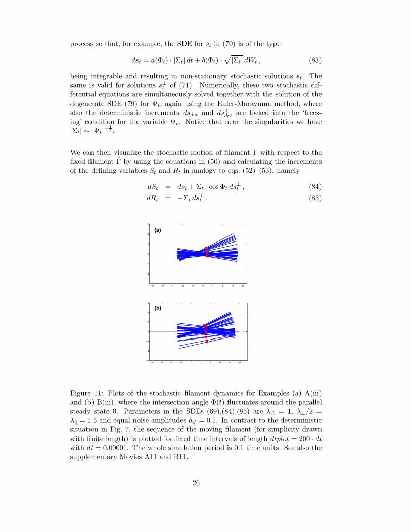
Figure 11: Plots of the stochastic filament dynamics for Examples (a) A(iii)and (b) B(iii), where the intersection angle Φ(t) fluctuates around the parallelsteady state 0. Parameters in the SDEs (69),(84),(85) are λ = 1, λ⊥/2 =λ‖ = 1.5 and equal noise amplitudes b# = 0.1. In contrast to the deterministicsituation in Fig. 7, the sequence of the moving filament (for simplicity drawnwith finite length) is plotted for fixed time intervals of length dtplot = 200 · dtwith dt = 0.00001. The whole simulation period is 0.1 time units. See also thesupplementary Movies A11 and B11.

26

−10 −5 0 5 10 15

−6

−4

−2

0

2

4

6 (a)

−10 −5 0 5 10 15

−6

−4

−2

0

2

4

6

(b)

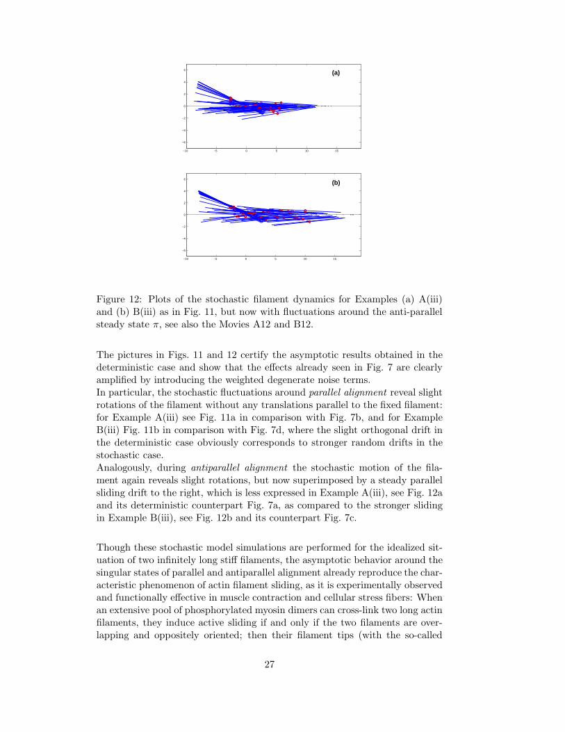
Figure 12: Plots of the stochastic filament dynamics for Examples (a) A(iii)and (b) B(iii) as in Fig. 11, but now with fluctuations around the anti-parallelsteady state π, see also the Movies A12 and B12.

The pictures in Figs. 11 and 12 certify the asymptotic results obtained in thedeterministic case and show that the effects already seen in Fig. 7 are clearlyamplified by introducing the weighted degenerate noise terms.In particular, the stochastic fluctuations around parallel alignment reveal slightrotations of the filament without any translations parallel to the fixed filament:for Example A(iii) see Fig. 11a in comparison with Fig. 7b, and for ExampleB(iii) Fig. 11b in comparison with Fig. 7d, where the slight orthogonal drift inthe deterministic case obviously corresponds to stronger random drifts in thestochastic case.Analogously, during antiparallel alignment the stochastic motion of the fila-ment again reveals slight rotations, but now superimposed by a steady parallelsliding drift to the right, which is less expressed in Example A(iii), see Fig. 12aand its deterministic counterpart Fig. 7a, as compared to the stronger slidingin Example B(iii), see Fig. 12b and its counterpart Fig. 7c.

Though these stochastic model simulations are performed for the idealized sit-uation of two infinitely long stiff filaments, the asymptotic behavior around thesingular states of parallel and antiparallel alignment already reproduce the char-acteristic phenomenon of actin filament sliding, as it is experimentally observedand functionally effective in muscle contraction and cellular stress fibers: Whenan extensive pool of phosphorylated myosin dimers can cross-link two long actinfilaments, they induce active sliding if and only if the two filaments are over-lapping and oppositely oriented; then their filament tips (with the so-called

27

‘barbed ends’ anchored in the Z-lines or the plasma membrane) move towardseach other so that, for instance, in a muscle cell the sarcomeres can eventuallybe contracted. The reason is that, as the model assumptions suppose, myosindimers preferentially bind to an actin filament with its head oriented towardsthe ‘barbed end’, see the model in Example A(iii) and Fig. 5b, and that un-der this condition they can also perform a stochastic power-stroke inducing apre-tension of their elastic ‘springs’ (between head and tail), see the additionalmodel assumptions in Example B(iii) and Fig. 5c.

We emphasize the difference between this ‘active’ dynamics and the simple neg-ative gradient flow dynamics as shown by the symmetric model A(i). There,also during stochastic motion of a filament pair, the mutual interaction energyalways tends to the (infinitely negative) energy minimum of alignment. In con-trast, for the asymmetric ‘myosin-like’ models A(iii) and B(iii) the additionalenergy, which is fed into the filament pair system due to preferential bindingand hydrolysis-mediated active force application by the cross-linkers, inducesthe additional phenomenon of angle-dependent filament sliding, an ‘active’ ef-fect that is superimposed onto the simple physical law of energy minimization.

As already mentioned in section 2, Fig. 2, the trace Cd of all possible cross-linker states of minimal length is an ellipse along one of the diagonals s =sors = −s, increasing in size proportionally to 1/| sinϕ| as the intersectionangle |ϕ| or |π−ϕ| between the filaments becomes smaller. This means nothingelse than that, in the same manner, the filament part carrying bound cross-links increases in size. However, due to the model assumptions above, withthe amount of active cross-linkers also the variance of induced ‘molecular noise’likewise increases, so that the resulting stationary stochastic process shows avanishing probability of ‘true’ alignment. More precisely, as can be seen in theasymptotic histogram in Fig. 10b, small intersection angles very rarely occur,but there is a clear hump around a positive mean absolute angular deviation,which can be explicitly computed, with a finite expected value for the inversesine, namely E(| sin Φt|−1) <∞. This has the important consequence that alsothe mean number of active cross-linkers and the mean interval length of occu-pied binding sites on each filament stay finite during the fluctuating alignmentprocess.

Thus, although the hypothesis of infinite filament length, which has been sup-posed for the current model, induces a degenerate convergence of the determin-istic dynamics to complete alignment along the whole infinite filaments in finitetime, the implementation of an appropriately modeled and scaled stochasticnoise reverses this extreme behavior near the singularity and makes very smallintersection angles very rare, so that most of the time only finite parts of thefilaments are connected by cross-linkers.

Nevertheless, for applying these model results to biopolymer dynamics, the

28

additional effects due to finite filament length should be investigated, which isbriefly undertaken in the following last section.

5 Dynamics of a filament with finite length

In order to explore the effects due to a more realistic modeling of semi-flexiblefilaments as stiff rods having finite length, we consider the simplified situationof pairing a short filament with a relatively long filament. Therefore, we couldassume that the longer filament stays fixed and that the smaller filament per-forms its ‘interaction dance’ on the middle part of this fixed filament, therebynot reaching its ends. Consequently, the fixed filament can be supposed asinfinitely long.

Under these conditions the forgoing model equations in section 3 have just tobe adapted in order to calculate torque and translation forces onto the movingfilament Γ. Again supposing that only the spring forces of cross-linkers comeinto action, then under the simplifying assumption made in Example B, namelythat the cross-link length is approximately constant, ρ ≡ d, the measure valuedversion of the local force kernel Kf = K(s, s) can be used as it appears in (40)and (31). However, the integration domain in the (s, s)-space is now restrictedto those parts of the ellipse Cd whose s-values lie on the filament, see Fig. 2. Letus remind that s denotes the arc length on filament Γ with s = 0 representingthe intersection point with the other filament. Choosing the mass center as fixedpoint (X(t), Y (t)) on the moving filament, then according to the terminologyin (50) the variable S = S(t) denotes the s-value of this center point, so thatwith finite filament length L the condition for s to represent an arbitrary pointon the filament is

|s− S| ≤ L

2. (86)

Since the integration in all torque and force integrals is performed only on thecurve Cd, the relevant s-values representing occupied cross-link binding sites,see (4), satisfy

|s| = |d · sin(ϕ+ α)

sinϕ| ≤ d

sinϕ, (87)

where we again restrict the derivation of this formula to the case 0 < ϕ < π.For all these s-positions except the extreme ones, there are two angles α andα = π − 2ϕ − α, under which cross-linkers can bind, see Figs. 1 and 2. Thenthe twofold integration domain is given by the intersection of both conditions(86) and (87) yielding s−(ϕ, S) ≤ s ≤ s+(ϕ, S) with

s±(ϕ, S) = ±min(d

sinϕ,L

2± S) . (88)

Transformation into the α-parametrization, using the property

ds = cos(ϕ+ α)d

sinϕdα (89)

29

gives a well-determined integration domain α ∈ Aϕ,S and a ‘symmetry-map’α 7→ α with the property sin(ϕ + α) = sin(ϕ + α), so that both angles belongto the same binding site s and that any of the integral representations with akernel g = gϕ(α) as in eqs. (43)–(45) can be written as a twofold integral overs, expressed by the sum of two integrands, namely gϕ(α) and gϕ(α):

d

sinϕ

∫

Aϕ,S

gϕ(α) dα =

∫ s+(ϕ,S)

s−

(ϕ,S)

gϕ(α) + gϕ(α)

cos(ϕ+ α)ds

=d

sinϕ

∫ r+(ϕ,S)

r−

(ϕ,S)

gϕ(α) + gϕ(α)√1 − r2

dr . (90)

In the last integral transformation we have used the substitution of s in (4) bythe ‘normalized’ variable

r = sin (ϕ+ α) =sinϕ

ds (91)

with integration domain limited by

r+(ϕ, S) = min

1,

sinϕ

d

(S +

L

2

)(92)

r−(ϕ, S) = max

−1,

sinϕ

d

(S − L

2

). (93)

In dependence of the occurring angles α, α = π−ϕ−α and α = π−2ϕ−α withthe properties ˜α = α+ϕ and α = α−ϕ we can state the following formulas forthe trigonometric functions, by using the subsidiary function Qr :=

√1 − r2,

sin α = sin ˜α = r

cos α = − cos ˜α = −Qr

sinα = r cosϕ−Qr sinϕ ; cosα = r sinϕ+Qr cosϕ

sin α = r cosϕ+Qr sinϕ ; cos α = r sinϕ−Qr cosϕ .

With the aid of these formulas the integral in (90) over r for any of the torqueand force representations in section 3 can be explicitly calculated in terms ofthe integration limits. For computing the torque, for instance, in the case ofinfinitely long filaments the virtual rotation was performed around the inter-section point, which now has to be replaced by the mass center. Thus, usinga generalized version of (41) provides the following integral representation forthe total torque onto filament Γ:

Ω(ϕ, S) =

∫

Γ

∫

eΓ(s− S) θ⊥ ·Kf ds ds

=h/2π

sinϕ

∫

Aϕ,S

kϕ(α)

(d

sinϕsin α− S

)sinα q(α) q(α) dα . (94)

Similar representations can be obtained for the forces F ‖ and F⊥.

30

Let us define the second auxiliary function Gr = 1π (arcsin(r) − r Qr), being an

odd function on the maximal integration interval [−1, 1] with infinite slope atr = ±1 and flat asymptotics Gr ∼ 2

3π r3 near r = 0. Then we obtain for

Example A(i) with infinitely stiff cross-linkers:

Ω(ϕ, S) = −2κ0cosϕ

sinϕ

(d

sinϕ

1

2[Gr+(ϕ,S) −Gr

−(ϕ,S)] −

S

π[Qr

−(ϕ,S) −Qr+(ϕ,S)]

),

F ‖(ϕ, S) = −2κ0

π[Qr

−(ϕ,S) −Qr+(ϕ,S)] ,

F⊥(ϕ, S) = −2κ0

π

1

tanϕ[Qr

−(ϕ,S) −Qr+(ϕ,S)] .

In general, the ODEs for the three dynamic variables Φ(t), S(t) and R(t) canbe taken as in (51)–(53), now with the nonlinearities also depending on S(t)and, clearly, on the length L of the filament (including the inverse frictioncoefficients). The consequence is that now the first two differential equationsconstitute a nonlinearly coupled ODE system:

dΦ

dt= λ Ω(Φ, S) , (95)

dS

dt= λ FS(Φ, S) := λ‖ F

‖(Φ, S) +λ⊥

tan ΦF⊥(Φ, S) . (96)

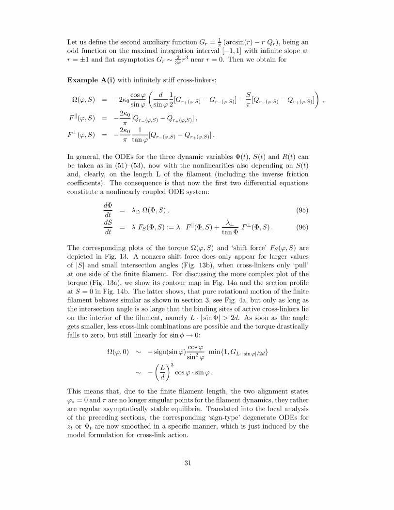
The corresponding plots of the torque Ω(ϕ, S) and ‘shift force’ FS(ϕ, S) aredepicted in Fig. 13. A nonzero shift force does only appear for larger valuesof |S| and small intersection angles (Fig. 13b), when cross-linkers only ‘pull’at one side of the finite filament. For discussing the more complex plot of thetorque (Fig. 13a), we show its contour map in Fig. 14a and the section profileat S = 0 in Fig. 14b. The latter shows, that pure rotational motion of the finitefilament behaves similar as shown in section 3, see Fig. 4a, but only as long asthe intersection angle is so large that the binding sites of active cross-linkers lieon the interior of the filament, namely L · | sin Φ| > 2d. As soon as the anglegets smaller, less cross-link combinations are possible and the torque drasticallyfalls to zero, but still linearly for sinφ→ 0:

Ω(ϕ, 0) ∼ − sign(sinϕ)cosϕ

sin2 ϕmin1, GL·| sinϕ|/2d

∼ −(L

d

)3

cosϕ · sinϕ .

This means that, due to the finite filament length, the two alignment statesϕ∗ = 0 and π are no longer singular points for the filament dynamics, they ratherare regular asymptotically stable equilibria. Translated into the local analysisof the preceding sections, the corresponding ‘sign-type’ degenerate ODEs forzt or Ψt are now smoothed in a specific manner, which is just induced by themodel formulation for cross-link action.

31

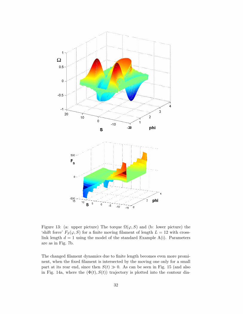
Figure 13: (a: upper picture) The torque Ω(ϕ, S) and (b: lower picture) the‘shift force’ FS(ϕ, S) for a finite moving filament of length L = 12 with cross-link length d = 1 using the model of the standard Example A(i). Parametersare as in Fig. 7b.

The changed filament dynamics due to finite length becomes even more promi-nent, when the fixed filament is intersected by the moving one only for a smallpart at its rear end, since then S(t) ≫ 0. As can be seen in Fig. 15 (and alsoin Fig. 14a, where the (Φ(t), S(t)) trajectory is plotted into the contour dia-

32

phi

S

0.5 1 1.5 2 2.5 3

−10

−5

0

5

10(a)

0 0.5 1 1.5 2 2.5 3−20

−15

−10

−5

0

5

10

15

20

phi

Ω( . ,0)

(b)

Figure 14: (a) Contour lines of the torque Ω(ϕ, S) together with a specifictrajectory of eqs. (95)–(96), and (b) profile of Ω(ϕ, 0) for the situation whenthe intersection point is the mass center of the moving filament, see the textfor comparison with the corresponding plot in Fig. 4a.

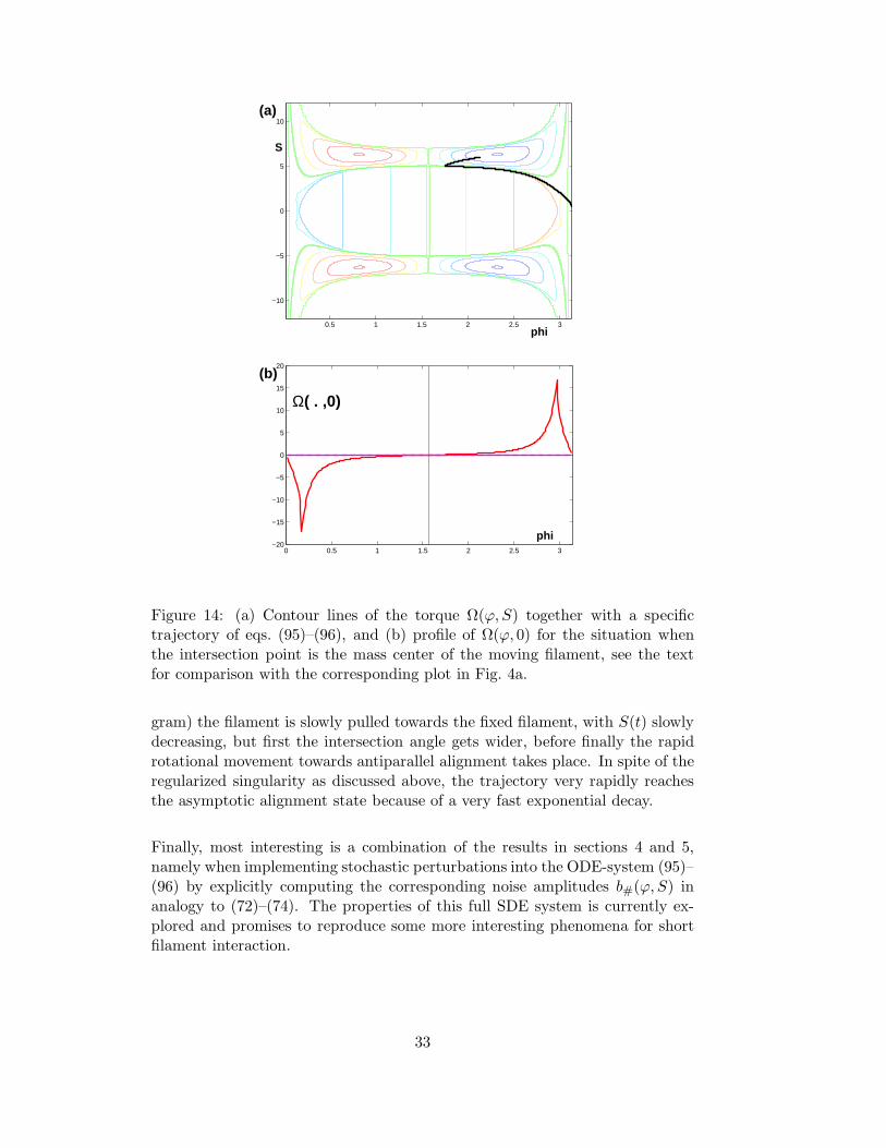
gram) the filament is slowly pulled towards the fixed filament, with S(t) slowlydecreasing, but first the intersection angle gets wider, before finally the rapidrotational movement towards antiparallel alignment takes place. In spite of theregularized singularity as discussed above, the trajectory very rapidly reachesthe asymptotic alignment state because of a very fast exponential decay.

Finally, most interesting is a combination of the results in sections 4 and 5,namely when implementing stochastic perturbations into the ODE-system (95)–(96) by explicitly computing the corresponding noise amplitudes b#(ϕ, S) inanalogy to (72)–(74). The properties of this full SDE system is currently ex-plored and promises to reproduce some more interesting phenomena for shortfilament interaction.

33

−15 −10 −5 0 5

−4

−2

0

2

4

6

8

10

12(a)

0 1 2 3 4 5 6−6

−4

−2

0

2

4

6

Φt

Ψt

St

π − Rt

(b)

Figure 15: Deterministic dynamics of a finite moving filament on a fixed in-finite filament (the x-axis) for model A(i) with parameters and conditions asin Fig. 13. In (a: upper picture) the filament finally aligns antiparallelly, butthe intersection angle π − Φt first increases towards π/2 while the filament ispulled down, before the angle rapidly adjusts to alignment, see the dark curvein (b: lower picture) and Movie A15. The convergence of Φt → π as well as ofthe two other variables St and Rt towards a steady state is not performed infinite time: due to the smoothed Ω function (see Fig. 14b) there remain tinydeviations that are exponentially decreasing, though with a fast rate of order(L/d)3 = 123 in our case.

6 Summary and further applications

The most important feature of the presented continuum model, for the inter-action between stiff filaments, is the possibility to derive explicit local forcekernels for a variety of applicable cross-linking mechanisms, which then can beused to calculate torques and translational forces between the ‘rods’ as explicitglobal integrals depending only on the geometric constellation. Clearly, this isvalid only under the assumed hypothesis that there is a continuum of potential

34

cross-link binding sites and a pseudo-stationary equilibrium in the Poisson pro-cess of binding and unbinding. However, not only the mean binding strength independence of the geometric variables is condensed into a deterministic model;also the stochastic fluctuations are modeled and simulated according to an ap-propriate Gaussian noise kernel in the global integrals. Then, stochastic inte-gration provides explicit variance expressions for the additive stochastic torquesand forces, leading to a system of degenerate stochastic differential equations(SDEs) for the filament variables (position and direction).

So far we have restricted the derivation of local force kernels to the case that stiffcross-linkers (as e.g. myosin dimers) apply forces only in direction of their ‘con-nection vector’. However, many cross-linking polymers could be bent or twisted(as filamin, fascin or α-actinin) and thus could exert torque moments onto theattached filaments (see e.g. [24],[18]). Under suitable model assumptions on thetype and angular dependence of cross-linker micromechanics, analogous explicitkernels for the corresponding forces (Kω and Kω in our notation) can then bederived. Obviously, the resulting degenerate differential equations could havedifferent asymptotics and reveal a variety of other convergence and fluctuationproperties.

As one advantage of this simplified model we have demonstrated a thoroughasymptotic analysis around the singular states of parallel and antiparallel align-ment, from which some basic properties of the stochastic processes can be quan-titatively extracted. Moreover, the presented regularization procedures are alsoused for consistent numerical procedures to simulate the degenerate stochasticdynamics, which reveals typical properties of actin filament sliding in the casethat ‘contractile’ myosin dimers act as cross-linkers.

As a further advantage, the explicitly computable (deterministic and stochastic)integrals could be easily used for more realistic worm-like-chain (WLC) modelsof longer semi-flexible filaments, if just applied to all possible pair interactionsbetween piecewise straight segments of the discretized filaments. The resultingnumerical algorithms, which reflect the approximative pseudo-stationary cross-linking process, could well compete with so far used ‘molecular dynamics’ sim-ulations that uses multi-particle methods to represent individual cross-linkers(see e.g. [15]), particulary when applied to whole networks of interacting fila-ments as they currently are observed in experiments, see [1], for instance.

Moreover, for the real 3-dimensional biological system of semi-flexible actin fil-aments, most of the 2-dimensional dynamic properties presented here can becarried over and used as a basic description for more generalized interactionmodel: There is an additional degree of freedom not only in filament rotationand bending, but also in parametrizing the space angles of cross-link binding.Finally, we hope that an application of our approach, namely to derive explicitlocal interaction kernels from detailed molecular mechanisms on a microscale,

35

could give an input to the improvement or new development of more physio-logical (than purely phenomenological) continuum models for thermodynamicaland fluid dynamical theories of polymer networks (see e.g. [2] or [10]), particu-larly for modeling and simulating the contractile actin-myosin cytoskeleton inbiological cells (see [12]).

AcknowledgementWe thank the DFG for generously supporting this research, particularly withinthe Special Research Program (SFB 611) on Singular Phenomena and Scalingin Mathematical Models at Bonn University.

Supplementary materialVisualization of the stochastic filament dynamics depicted in Figs. 11, 12 and15 in a form of picture sequences (Movies [A11, B11], [A12, B12] and A15) willbe available under www.theobio.uni-bonn.de\~filaments-stochastic.

References

[1] P.M. Bendix et al. and D.A. Weitz. A quantitative analysis of con-tractility in active cytoskeletal protein networks. Biophys. J. 94:3126–3136, 2008.

[2] I. Borukhov, R.F. Bruinsma, W.M. Gelbart and A.J. Liu. Struc-tural polymorphism of the cytoskeleton: a model of linker-assistedfilament aggretation. Proc. Natl. Acad. Sc. USA 102: 3673–3678,2005.

[3] S. Blatt and P. Reiter. Does finite knot energy lead to differentia-bility? Preprint no. 12, Institut fur Mathematik, RWTH Aachen2006; see http://www.instmath.rwth-aachen.de/→ preprints.

To appear in J. Knot Theory Ramifications.

[4] J. Cantarella, M. Piatek and E. Rawdon. Visualizing the tighteningof knots. In: VIS’05: Proc. of the 16th IEEE Visualization 2005,pp. 575–582. IEEE Computer Society, Washington, DC, 2005.

[5] M.H. Freedman, Zheng-Xu He and Zhenghan Wang. Mobius energyof knots and unknots. Ann. of Math.(2), 139(1): 1–50, 1994.

[6] O. Gonzalez, J.H. Maddocks, F. Schuricht and H. von der Mosel.Global curvature and self-contact of nonlinearly elastic curves androds. Calc. Var. Partial Differential Equations, 14(1): 29–68, 2002.

[7] Zheng-Xu He. The Euler-Lagrange equation and heat flow for theMobius energy. Comm. Pure Appl. Math., 53(4): 399–431, 2000.

36

[8] S. Highsmith. Lever arm model for force generation by actin-myosin-ATP. Biochemistry 38: 791-797, 1999.

[9] L.W. Janson and D.L. Taylor. Actin-crosslinking protein regula-tion of filament movement in motility assays: a theoretical model.Biophys. J. 67: 973-982, 1994.

[10] J.F. Joanny, F. Julicher, K. Kruse and J. Prost. Hydrodynamictheory for multicomponent active polar gels. New J. Phys. 9: 422,2007.

[11] P.E. Kloeden and E. Platen. Numerical Solution of Stochastic Dif-ferential Equations. Springer, Berlin, 1992.

[12] S.A. Koestler, S. Auinger, M. Vinzenz, K. Rottner and J.V. Small.Differentially oriented populations of actin filaments generated inlamellipodia collaborate in pushing and pausing at the cell front.Nature Cell Biol. 10.1038/ncb1692, 2008.

[13] R.B. Kusner and J.M. Sullivan. Mobius-invariant knot energies. In[22], pp. 315–352, 1998.

[14] Xiumei Liu and G.H. Pollack. Stepwise sliding of single actin andmyosin filaments. Biophys. J. 86: 353-358, 2004.

[15] F. Nedelec. Computer simulations reveal motor properties gener-ating stable antiparallel microtubule interaction. J. Cell Biol. 158:1005–1015, 2002.

[16] J. O’Hara. Energy of a knot. Topology, 30(2): 241–247, 1991.

[17] J. O’Hara. Energy of knots and conformal geometry. Vol. 33 of:Series on Knots and Everything. World Scientific Publishing Co.Inc., River Edge, NJ, 2003.

[18] O. Peletier et al. and C.R. Safinya. Structure of actin cross-linkeswith α-actinin: a network of bundels. Phys. Rev. Letters 91(14):148102, 2003.

[19] P. Reiter. Knotenenergien. Diploma thesis, Math. Inst. Univ. Bonn,2004.

[20] P. Reiter. On repulsive knot energies. PhD thesis, RWTH Aachen,to appear in Oct. 2008.

[21] F. Schuricht and H. von der Mosel. Characterization of ideal knots.Calc. Var. Partial Differential Equations 19: 281–305, 2004.

[22] A. Stasiak, V. Katritch and L.H. Kauffman, editors. Ideal knots.Vol. 19 of: Series on Knots and Everything. World Scientific Pub-lishing Co. Inc., River Edge, NJ, 1998.

37

[23] P. Strzelecki and H. von der Mosel. On rectifiable curves with Lp-bounds on global curvature: Self-avoidance, regularity, and mini-mizing knots. Math. Z. 257: 107–130, 2007.

[24] J. Ylanne, K. Scheffzek, P. Young and M. Saraste. Crystal structureof the α-actinin rod reveals an extensive torsional twist. Structure9: 597–604, 2001.

38