institutions and economic growth: in search of robustness witkowski... · 1 mariusz próchniak,...
TRANSCRIPT

1
Mariusz Próchniak, Bartosz Witkowski
WARSAW SCHOOL OF ECONOMICS (POLAND)
Institutions and Economic Growth: In Search of Robustness
Mariusz Próchniak, Ph.D.Department of Economics II, Warsaw School of Econom ics
Al. Niepodległo ści 162, 02-554 Warszawa, PolandE-mail: [email protected]
Bartosz Witkowski, Ph.D.Institute of Econometrics, Warsaw School of Economic s
Al. Niepodległo ści 162, 02-554 Warszawa, PolandE-mail: [email protected]
This research project has been financed by the Nati onal Bank of Poland within the frame of the competition for research grants scheduled fo r 2013.
2
1. Introduction
2. Review of the literature
3. Bayesian model averaging
4. Data
5. Results
6. Conclusions
References
CONTENTS

2
3
MOTIVATION
• Many papers on the impact of the regulatory framework oneconomic growth have emerged in recent years. The conclusionsobtained by various authors depend on the analyzed sample,model specification, and the estimation method.
• Some questions are not solved yet (whether the relationship islinear or nonlinear; what freedoms contribute the most toeconomic growth; or what is the strength of the impact)?
• Sala-i-Martin, Doppelhofer, and Miller (SDM, 2004) use Bayesianaveraging of classical estimates (BACE) approach. Instead ofusing one model, they estimate a large number of equationscorresponding to numerous possible sets of explanatory variableschosen from an initially selected group of ‘candidate-variables’.The results are then averaged using specified weights.
• This study applies the SDM approach to the Blundell and Bond’sGMM system estimator.
4
THE AIMS OF THE ANALYSIS
• To analyze the relationship between regulatory variables(economic freedom, quality of governance, democracy level, doingbusiness indicators, transition indicators) and economic growth.
• Focus on:
� nonlinear impact;� level of and change in the regulatory variables;� components of the aggregated indices.
• The analysis is mostly based on ‘overlapping’ panel data in theform of 5- or 10-year subperiod averages.
• The analysis covers the 1970-2012 period and the following groupsof countries:
� world economies (max. 171);� EU27 countries;� post-socialist countries.

3
5
BACKGROUND – empirical evidence (1/4)
• De Haan et al. (2006): wide review of empirical studies on therelationship between economic freedom and economic growth(more than 30 empirical studies).
⇒⇒⇒⇒ Economic freedom is important in explaining differences ineconomic performance, however most studies have seriousdrawbacks, including lacking sensitivity analysis and poorspecifications of the growth model.
• Pääkkönen (2010): 25 transition economies, 1998-2005,relationship between economic freedom and economic growth.
⇒⇒⇒⇒ Growth researchers should test for the presence ofnonlinearities.
• Bergh and Karlsson (2010): 29 OECD countries, 1970-1995.
⇒⇒⇒⇒ Unexpectedly, the idea that economic freedom matters haslittle support.
6
BACKGROUND – empirical evidence (2/4)
• Justesen (2008): causal relationship between economic freedomand economic growth using the Granger causality tests.
⇒ At least some aspects of economic freedom are importantdeterminants of GDP growth; the analysis raises doubts as towhether all dimensions of economic freedom matter.
⇒ Hence, analysis of component indicators is important.
• Aixalá and Fabro (2009): causality between economic growthand: economic freedom, civil liberties and political rights.
⇒ Bilateral causality between economic freedom, civil libertiesand growth; when the analysis works with changes (notlevels), only the relation between changes in economicfreedom and growth is significant and also bilateral.
⇒ It is appropriate to analyze both the level of and the change ininstitutional variables; bilateral relationship justifies thetreatment of regulatory variables as endogenous.

4
7
BACKGROUND – empirical evidence (3/4)
• Peev and Mueller (2012): the interrelationships betweendemocracy, economic freedoms, and economic growth.
⇒ Trade freedom, monetary freedom and freedom fromcorruption are the most important economic growthdeterminants in transition countries; democracy can have alsoan adverse effect on economic growth, by producing largerpublic sectors and public deficits.
⇒ It is worth to carry out a more advanced analysis coveringmore countries and aiming to find which areas of freedomaffect mostly economic growth and whether some negativeeffects between institutional variables (like democracy) andeconomic growth are indeed evidenced.
8
BACKGROUND – empirical evidence (4/4)
• Some other studies described in the report:
� Heckelman and Knack (2009)
� Azman-Saini, Baharumshah, and Law (2010)
� Compton, Giedeman, and Hoover (2011)
� Williamson and Mathers (2011)
� Fabro and Aixalá (2012)

5
• Problem 1: in growth models there are hardly any „sure” independent variables and no single specification is obvious.
� Apply Bayesian Model Averaging: estimate models with allpossible subsets of the candidate independent variables, thenaverage the results using posterior probability weights.
• Problem 2: the relationship need not be linear.
���� Introduce squares of institutional environment variables.
• Problem 3: equations are autoregressive.
���� Use Blundell and Bond method of estimation.
• Problem 4: series in the panel of countries are short and there arefew observations to use GMM in a reasonable way.
� Use overlapping periods: e.g. t=1 covers period 1991-1995, t=2 covers period 1992-1996, t=3 covers 1993-1997; since for the dependent variable we use only the starting and ending valuethese are not redundant.
ECONOMETRIC SOLUTION
9
• Prior probability of model Mj (assumption!):
• Posterior probability with the use of dataset D:
• Problem with computation:
• Finally with GMM estimation:
• Estimates of „influence” parameters:
( ) ( ) jj KK
KkK
Kk
jM−
−= 1)(P
∑=
=J
iii
jjj
MDM
MDMDM
1
)|(P)(P
)|(P)(P)|(P
∫= jjjjj MDMD θθθ d)|(P),(L)|(P
∑=
−
−
−
−=
J
ii
Ki
jK
jj
nnM
nnMDM
i
j
1
2/'
2/'
])ˆQ(5.0exp[)P(
])ˆQ(5.0exp[)P()|P(
θ
θ
∑=
=J
jjrjr β|DM
1,
ˆ)(Pβ̂ ∑∑==
−⋅+⋅=J
jrjrj
J
jjrjr β|DM|DM
1
2,
1, )ˆˆ()P()ˆVar()P()ˆ(Var βββ
10
MAIN FORMULAS OF BAYESIAN MODEL AVERAGING

6
MAIN FORMULAS
∆������� = � + ������,�� + �′�� + �� + ���
������� = � + ( +1)������,�� + �′�� + �� + ���
11
• The classical Barro regression:
• The transformed model:
DATA
12
Regulations (institutions) are measured by the following indicators:
• the Heritage Foundation index of economic freedom,
• the Fraser Institute index of economic freedom,
• the World Bank worldwide governance indicators,
• the Freedom House democracy index,
• the World Bank doing business indicators,
• the EBRD transition indicators.
Institutional variables are included:
• as the overall indicator or the component indicators,
• as the level (arithmetic average of the values recorded over agiven subperiod) or the change (between the initial and the finalyear of a given subperiod).
All the institutional variables are also included in a squared form.

7
13
DATA
• The explained variable - economic growth:
Change in GDP per capita at purchasing power parity (PPP) inconstant prices.
Source: PWT.
• All the regression equations include regulatory variables:
• the aggregated index or the component indicators (the latterones randomly chosen).
• Since it is believed that there does exist the beta-convergence,initial GDP per capita also appears in each estimated equation.
Table 1 Analyzed models (in the BMA sense)
Model no.
Regulatory variable(s) Data
transformation
Heritage Foundation
1 Level of the index of economic freedom 5-year overlapping panel
2 Levels of the components of the index of economic freedom 3 Change in the index of economic freedom 4 Changes in the components of the index of economic freedom
Fraser Institute
5 Level of the index of economic freedom 10-year overlapping panel
6 Change in the index of economic freedom 7 Levels of the components of the index of economic freedom 8 Changes in the components of the index of economic freedom
World Bank
9 Level of the worldwide governance indicator 5-year overlapping panel
10 Levels of the components of the worldwide governance indicator 11 Change in the worldwide governance indicator 12 Changes in the components of the worldwide governance indicator
Freedom House
13 Level of the democracy index 10-year overlapping panel
14 Levels of the components of the democracy index and freedom of the press 15 Change in the democracy index 16 Changes in the components of the democracy index and freedom of the press
World Bank
17 Levels of the doing business indicators Cross-sectional data 18 Changes in the doing business indicators
EBRD
19 Level of the transition indicator 5-year overlapping panel
20 Levels of the components of the transition indicator 21 Change in the transition indicator 22 Changes in the components of the transition indicator

8
Table 2 The list of control variables
Name Description Typea
lngdp0 Lagged log GDP per capita at PPP (constant prices) E inv Investment (% of GDP) E school_tot Average years of total schooling (population ages 15+) E school_ter Percentage of population (ages 15+) with completed tertiary education E edu_exp Education expenditure (% of GNI) E gov_cons General government consumption expenditure (% of GDP) E gov_rev General government revenue (% of GDP) E gov_bal General government balance (% of GDP) E open Openness ((exports + imports) / GDP) E cab Current account balance (% of GDP) E fdi Net FDI inflow (% of GDP) E
cred Annual change (in % points) of the domestic credit provided by banking sector in % of GDP
E
inf Inflation (annual %) E serv Services value added (% of GDP) E life Log of life expectancy at birth (years) X fert Log of fertility rate (births per woman) X pop_15_64 Population ages 15-64 (% of total) X pop_den Log of population density (people per sq. km of land area) X pop_gr Population growth (annual %) X pop_tot Log of population, total X
a E – endogenous variable; X – exogenous variable.
Table 3 Control variables included in the respective BMA models
Variable Model
1-4 Model
5-8 Model 9-12
Model 13-16
Model 17-18
Model 19-22
lngdp0 x x x x x x inv x x x x x x school_tot x x
x
school_ter x x
x
edu_exp x
x x
gov_cons x x x x x x gov_rev
x
x
gov_bal
x
x
open x x x x x x cab
x
fdi x
x x x
cred x
x x
inf x x x x x
serv
x
life x x x x x
fert x x x x x
pop_15_64 x x x x x x pop_den x
x x x x
pop_gr x x x x x x pop_tot x x x x x x
“x” means that a given variable is included.

9
Table 5 Data coverage of the respective BMA models
Model Number
of observations Number
of countries
Number of observations
per country (avg.) Maximum perioda
1 1856 134 13.9 (1992)1997-2012 2 1856 134 13.9 (1992)1997-2012 3 1500 129 11.6 (1995)2000-2012 4 1500 129 11.6 (1995)2000-2012 5 2584 111 23.3 (1970)1980-2010 6 2584 111 23.3 (1970)1980-2010 7 2136 110 19.4 (1970)1980-2010 8 2136 110 19.4 (1970)1980-2010 9 1985 160 12.4 (1993)1998-2012 10 1985 160 12.4 (1993)1998-2012 11 1557 160 9.7 (1996)2001-2011 12 1557 160 9.7 (1996)2001-2011 13 2726 123 22.2 (1970)1980-2012 14 1569 122 12.9 (1988)1998-2012 15 2535 123 20.6 (1972)1982-2011 16 989 119 8.3 (1993)2003-2011 17 154 154 1 2005-2012 18 154 154 1 2005-2012 19 456 27 16.9 (1989)1994-2012 20 456 27 16.9 (1989)1994-2012 21 456 27 16.9 (1989)1994-2012 22 456 27 16.9 (1989)1994-2012
a The earliest year for which initial GDP is included (in the case of panel data) is given in brackets.
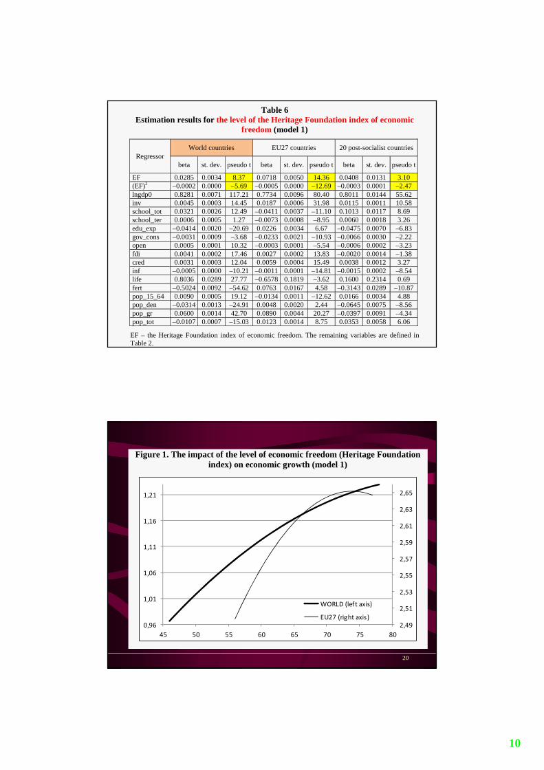
RESULTS – ECONOMIC FREEDOM
• Economic freedom contributes to economic growth.
• Countries with greater scope of economic freedom record onaverage the more rapid output growth.
• This relationship is nonlinear and statistically significant.
• The most beneficial effect on economic growth appears in thecountries with low scope of economic freedom: making thecountry more economically free has greater benefit in terms ofoutput acceleration if the level of economic freedom is low.
18
10
Table 6 Estimation results for the level of the Heritage Foundation index of economic
freedom (model 1)
Regressor World countries EU27 countries 20 post-socialist countries
beta st. dev. pseudo t beta st. dev. pseudo t beta st. dev. pseudo t
EF 0.0285 0.0034 8.37 0.0718 0.0050 14.36 0.0408 0.0131 3.10 (EF)2 –0.0002 0.0000 –5.69 –0.0005 0.0000 –12.69 –0.0003 0.0001 –2.47 lngdp0 0.8281 0.0071 117.21 0.7734 0.0096 80.40 0.8011 0.0144 55.62 inv 0.0045 0.0003 14.45 0.0187 0.0006 31.98 0.0115 0.0011 10.58 school_tot 0.0321 0.0026 12.49 –0.0411 0.0037 –11.10 0.1013 0.0117 8.69 school_ter 0.0006 0.0005 1.27 –0.0073 0.0008 –8.95 0.0060 0.0018 3.26 edu_exp –0.0414 0.0020 –20.69 0.0226 0.0034 6.67 –0.0475 0.0070 –6.83 gov_cons –0.0031 0.0009 –3.68 –0.0233 0.0021 –10.93 –0.0066 0.0030 –2.22 open 0.0005 0.0001 10.32 –0.0003 0.0001 –5.54 –0.0006 0.0002 –3.23 fdi 0.0041 0.0002 17.46 0.0027 0.0002 13.83 –0.0020 0.0014 –1.38 cred 0.0031 0.0003 12.04 0.0059 0.0004 15.49 0.0038 0.0012 3.27 inf –0.0005 0.0000 –10.21 –0.0011 0.0001 –14.81 –0.0015 0.0002 –8.54 life 0.8036 0.0289 27.77 –0.6578 0.1819 –3.62 0.1600 0.2314 0.69 fert –0.5024 0.0092 –54.62 0.0763 0.0167 4.58 –0.3143 0.0289 –10.87 pop_15_64 0.0090 0.0005 19.12 –0.0134 0.0011 –12.62 0.0166 0.0034 4.88 pop_den –0.0314 0.0013 –24.91 0.0048 0.0020 2.44 –0.0645 0.0075 –8.56 pop_gr 0.0600 0.0014 42.70 0.0890 0.0044 20.27 –0.0397 0.0091 –4.34 pop_tot –0.0107 0.0007 –15.03 0.0123 0.0014 8.75 0.0353 0.0058 6.06
EF – the Heritage Foundation index of economic freedom. The remaining variables are defined in Table 2.
Figure 1. The impact of the level of economic freedom (Heritage Foundation index) on economic growth (model 1)
2,49
2,51
2,53
2,55
2,57
2,59
2,61
2,63
2,65
0,96
1,01
1,06
1,11
1,16
1,21
45 50 55 60 65 70 75 80
WORLD (left axis)
EU27 (right axis)
20
11
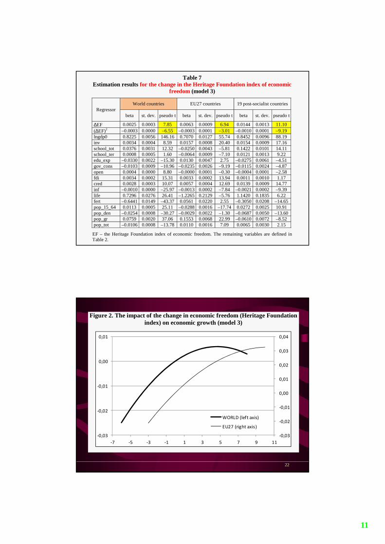
Table 7 Estimation results for the change in the Heritage Foundation index of economic
freedom (model 3)
Regressor World countries EU27 countries 19 post-socialist countries
beta st. dev. pseudo t beta st. dev. pseudo t beta st. dev. pseudo t
∆EF 0.0025 0.0003 7.85 0.0063 0.0009 6.94 0.0144 0.0013 11.10 (∆EF)2 –0.0003 0.0000 –6.55 –0.0003 0.0001 –3.01 –0.0010 0.0001 –9.19 lngdp0 0.8225 0.0056 146.16 0.7070 0.0127 55.74 0.8452 0.0096 88.19 inv 0.0034 0.0004 8.59 0.0157 0.0008 20.40 0.0154 0.0009 17.16 school_tot 0.0376 0.0031 12.32 –0.0250 0.0043 –5.81 0.1422 0.0101 14.11 school_ter 0.0008 0.0005 1.60 –0.0064 0.0009 –7.10 0.0121 0.0013 9.22 edu_exp –0.0330 0.0022 –15.30 0.0130 0.0047 2.75 –0.0275 0.0061 –4.51 gov_cons –0.0103 0.0009 –10.96 –0.0235 0.0026 –9.19 –0.0115 0.0024 –4.87 open 0.0004 0.0000 8.80 –0.0000 0.0001 –0.30 –0.0004 0.0001 –2.58 fdi 0.0034 0.0002 15.31 0.0033 0.0002 13.94 0.0011 0.0010 1.17 cred 0.0028 0.0003 10.07 0.0057 0.0004 12.69 0.0139 0.0009 14.77 inf –0.0010 0.0000 –25.97 –0.0013 0.0002 –7.84 –0.0021 0.0002 –9.39 life 0.7296 0.0276 26.41 –1.2265 0.2129 –5.76 1.1420 0.1835 6.22 fert –0.6441 0.0149 –43.37 0.0561 0.0220 2.55 –0.3050 0.0208 –14.65 pop_15_64 0.0113 0.0005 25.11 –0.0288 0.0016 –17.74 0.0272 0.0025 10.91 pop_den –0.0254 0.0008 –30.27 –0.0029 0.0022 –1.30 –0.0687 0.0050 –13.60 pop_gr 0.0759 0.0020 37.06 0.1553 0.0068 22.99 –0.0610 0.0072 –8.52 pop_tot –0.0106 0.0008 –13.78 0.0110 0.0016 7.09 0.0065 0.0030 2.15
EF – the Heritage Foundation index of economic freedom. The remaining variables are defined in Table 2.
Figure 2. The impact of the change in economic freedom (Heritage Foundation index) on economic growth (model 3)
-0,03
-0,02
-0,01
0,00
0,01
0,02
0,03
0,04
-0,03
-0,02
-0,01
0,00
0,01
-7 -5 -3 -1 1 3 5 7 9 11
WORLD (left axis)
EU27 (right axis)
22
12
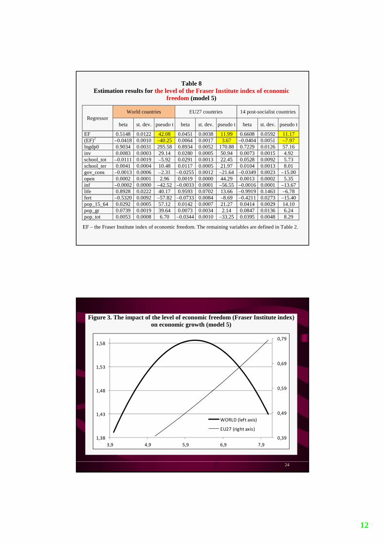
Table 8 Estimation results for the level of the Fraser Institute index of economic
freedom (model 5)
Regressor World countries EU27 countries 14 post-socialist countries
beta st. dev. pseudo t beta st. dev. pseudo t beta st. dev. pseudo t
EF 0.5148 0.0122 42.08 0.0451 0.0038 11.99 0.6608 0.0592 11.17 (EF)2 –0.0418 0.0010 –40.25 0.0064 0.0017 3.67 –0.0404 0.0051 –7.97 lngdp0 0.9034 0.0031 295.58 0.8934 0.0052 170.88 0.7229 0.0126 57.16 inv 0.0083 0.0003 29.14 0.0280 0.0005 50.94 0.0073 0.0015 4.92 school_tot –0.0111 0.0019 –5.92 0.0291 0.0013 22.45 0.0528 0.0092 5.73 school_ter 0.0041 0.0004 10.48 0.0117 0.0005 21.97 0.0104 0.0013 8.01 gov_cons –0.0013 0.0006 –2.31 –0.0255 0.0012 –21.64 –0.0349 0.0023 –15.00 open 0.0002 0.0001 2.96 0.0019 0.0000 44.29 0.0013 0.0002 5.35 inf –0.0002 0.0000 –42.52 –0.0033 0.0001 –56.55 –0.0016 0.0001 –13.67 life 0.8928 0.0222 40.17 0.9593 0.0702 13.66 –0.9919 0.1463 –6.78 fert –0.5320 0.0092 –57.82 –0.0733 0.0084 –8.69 –0.4211 0.0273 –15.40 pop_15_64 0.0292 0.0005 57.12 0.0142 0.0007 21.27 0.0414 0.0029 14.10 pop_gr 0.0739 0.0019 39.64 0.0073 0.0034 2.14 0.0847 0.0136 6.24 pop_tot 0.0053 0.0008 6.70 –0.0344 0.0010 –33.25 0.0395 0.0048 8.29
EF – the Fraser Institute index of economic freedom. The remaining variables are defined in Table 2.
Figure 3. The impact of the level of economic freedom (Fraser Institute index) on economic growth (model 5)
0,39
0,49
0,59
0,69
0,79
1,38
1,43
1,48
1,53
1,58
3,9 4,9 5,9 6,9 7,9
WORLD (left axis)
EU27 (right axis)
24
13
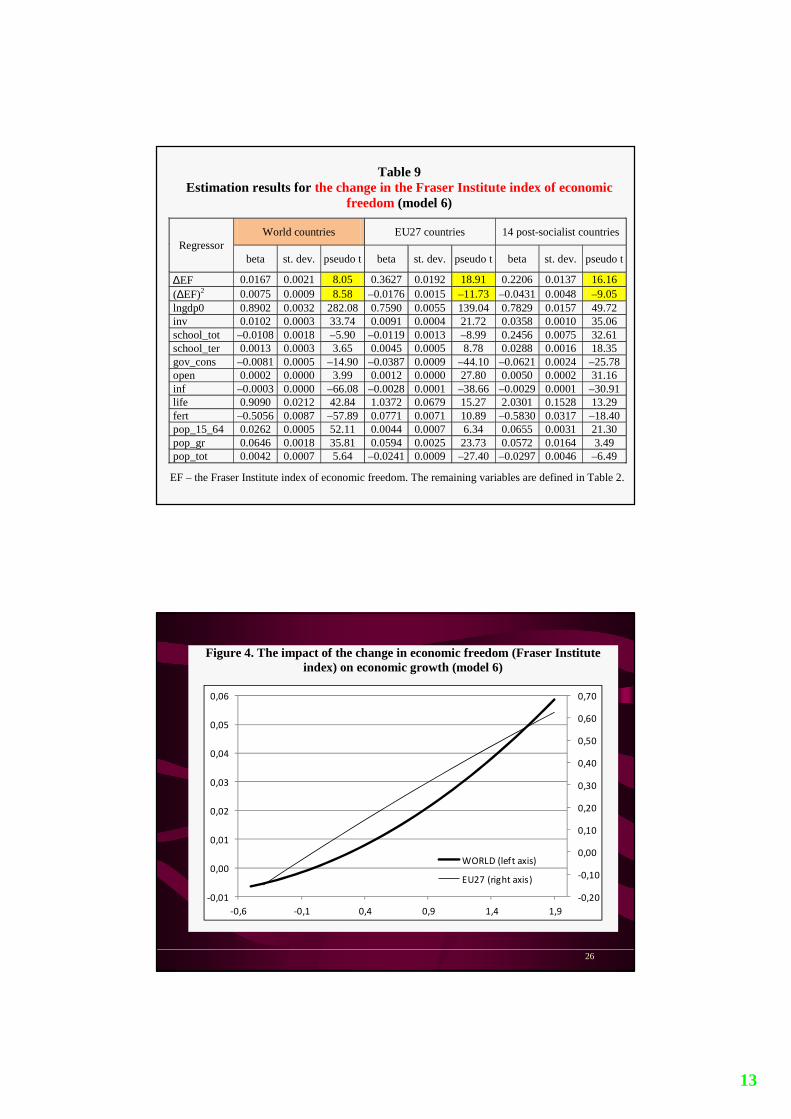
Table 9 Estimation results for the change in the Fraser Institute index of economic
freedom (model 6)
Regressor World countries EU27 countries 14 post-socialist countries
beta st. dev. pseudo t beta st. dev. pseudo t beta st. dev. pseudo t
∆EF 0.0167 0.0021 8.05 0.3627 0.0192 18.91 0.2206 0.0137 16.16 (∆EF)2 0.0075 0.0009 8.58 –0.0176 0.0015 –11.73 –0.0431 0.0048 –9.05 lngdp0 0.8902 0.0032 282.08 0.7590 0.0055 139.04 0.7829 0.0157 49.72 inv 0.0102 0.0003 33.74 0.0091 0.0004 21.72 0.0358 0.0010 35.06 school_tot –0.0108 0.0018 –5.90 –0.0119 0.0013 –8.99 0.2456 0.0075 32.61 school_ter 0.0013 0.0003 3.65 0.0045 0.0005 8.78 0.0288 0.0016 18.35 gov_cons –0.0081 0.0005 –14.90 –0.0387 0.0009 –44.10 –0.0621 0.0024 –25.78 open 0.0002 0.0000 3.99 0.0012 0.0000 27.80 0.0050 0.0002 31.16 inf –0.0003 0.0000 –66.08 –0.0028 0.0001 –38.66 –0.0029 0.0001 –30.91 life 0.9090 0.0212 42.84 1.0372 0.0679 15.27 2.0301 0.1528 13.29 fert –0.5056 0.0087 –57.89 0.0771 0.0071 10.89 –0.5830 0.0317 –18.40 pop_15_64 0.0262 0.0005 52.11 0.0044 0.0007 6.34 0.0655 0.0031 21.30 pop_gr 0.0646 0.0018 35.81 0.0594 0.0025 23.73 0.0572 0.0164 3.49 pop_tot 0.0042 0.0007 5.64 –0.0241 0.0009 –27.40 –0.0297 0.0046 –6.49
EF – the Fraser Institute index of economic freedom. The remaining variables are defined in Table 2.
Figure 4. The impact of the change in economic freedom (Fraser Institute index) on economic growth (model 6)
-0,20
-0,10
0,00
0,10
0,20
0,30
0,40
0,50
0,60
0,70
-0,01
0,00
0,01
0,02
0,03
0,04
0,05
0,06
-0,6 -0,1 0,4 0,9 1,4 1,9
WORLD (left axis)
EU27 (right axis)
26
14
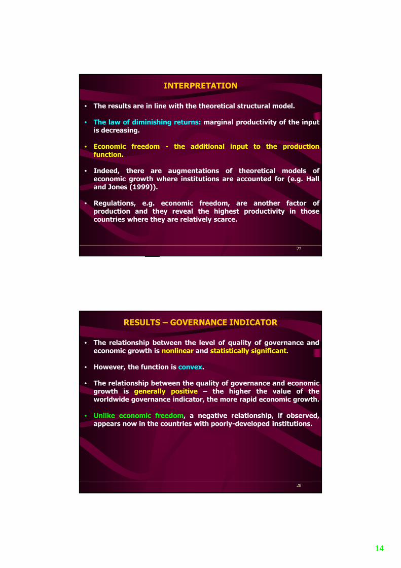
INTERPRETATION
• The results are in line with the theoretical structural model.
• The law of diminishing returns: marginal productivity of the inputis decreasing.
• Economic freedom - the additional input to the productionfunction.
• Indeed, there are augmentations of theoretical models ofeconomic growth where institutions are accounted for (e.g. Halland Jones (1999)).
• Regulations, e.g. economic freedom, are another factor ofproduction and they reveal the highest productivity in thosecountries where they are relatively scarce.
27
RESULTS – GOVERNANCE INDICATOR
• The relationship between the level of quality of governance andeconomic growth is nonlinear and statistically significant.
• However, the function is convex.
• The relationship between the quality of governance and economicgrowth is generally positive – the higher the value of theworldwide governance indicator, the more rapid economic growth.
• Unlike economic freedom, a negative relationship, if observed,appears now in the countries with poorly-developed institutions.
28
15
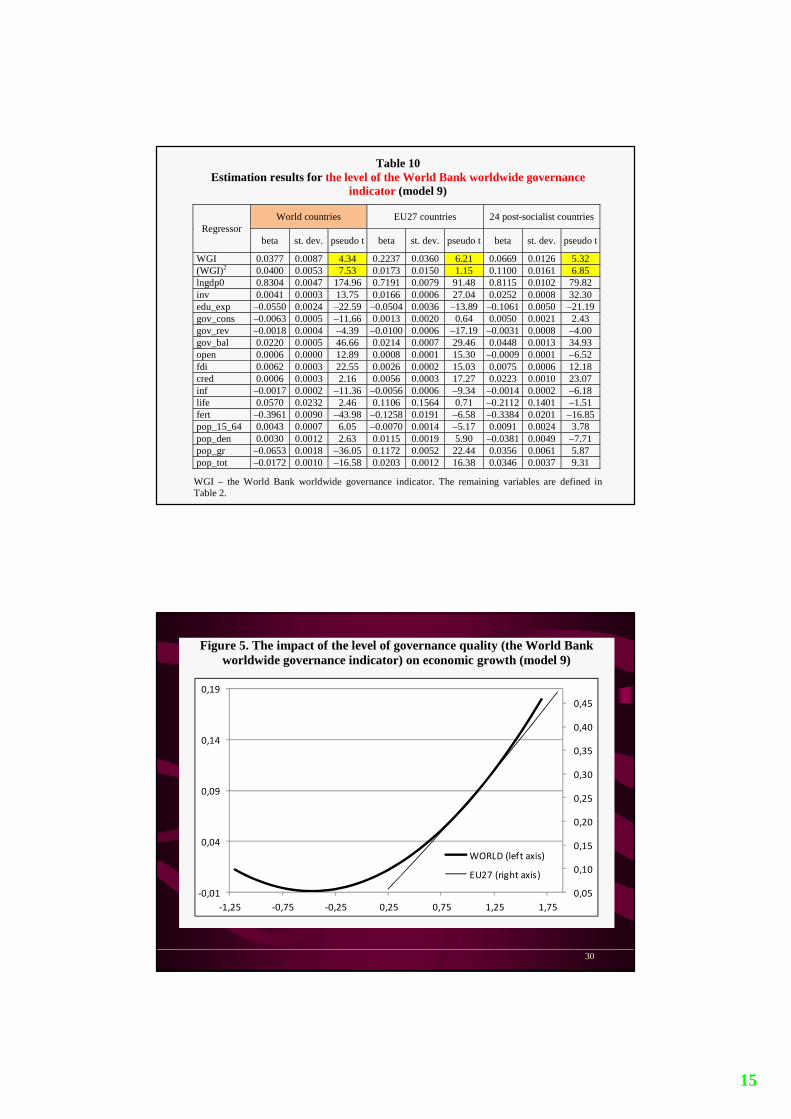
Table 10 Estimation results for the level of the World Bank worldwide governance
indicator (model 9)
Regressor World countries EU27 countries 24 post-socialist countries
beta st. dev. pseudo t beta st. dev. pseudo t beta st. dev. pseudo t
WGI 0.0377 0.0087 4.34 0.2237 0.0360 6.21 0.0669 0.0126 5.32 (WGI)2 0.0400 0.0053 7.53 0.0173 0.0150 1.15 0.1100 0.0161 6.85 lngdp0 0.8304 0.0047 174.96 0.7191 0.0079 91.48 0.8115 0.0102 79.82 inv 0.0041 0.0003 13.75 0.0166 0.0006 27.04 0.0252 0.0008 32.30 edu_exp –0.0550 0.0024 –22.59 –0.0504 0.0036 –13.89 –0.1061 0.0050 –21.19 gov_cons –0.0063 0.0005 –11.66 0.0013 0.0020 0.64 0.0050 0.0021 2.43 gov_rev –0.0018 0.0004 –4.39 –0.0100 0.0006 –17.19 –0.0031 0.0008 –4.00 gov_bal 0.0220 0.0005 46.66 0.0214 0.0007 29.46 0.0448 0.0013 34.93 open 0.0006 0.0000 12.89 0.0008 0.0001 15.30 –0.0009 0.0001 –6.52 fdi 0.0062 0.0003 22.55 0.0026 0.0002 15.03 0.0075 0.0006 12.18 cred 0.0006 0.0003 2.16 0.0056 0.0003 17.27 0.0223 0.0010 23.07 inf –0.0017 0.0002 –11.36 –0.0056 0.0006 –9.34 –0.0014 0.0002 –6.18 life 0.0570 0.0232 2.46 0.1106 0.1564 0.71 –0.2112 0.1401 –1.51 fert –0.3961 0.0090 –43.98 –0.1258 0.0191 –6.58 –0.3384 0.0201 –16.85 pop_15_64 0.0043 0.0007 6.05 –0.0070 0.0014 –5.17 0.0091 0.0024 3.78 pop_den 0.0030 0.0012 2.63 0.0115 0.0019 5.90 –0.0381 0.0049 –7.71 pop_gr –0.0653 0.0018 –36.05 0.1172 0.0052 22.44 0.0356 0.0061 5.87 pop_tot –0.0172 0.0010 –16.58 0.0203 0.0012 16.38 0.0346 0.0037 9.31
WGI – the World Bank worldwide governance indicator. The remaining variables are defined in Table 2.
Figure 5. The impact of the level of governance quality (the World Bank worldwide governance indicator) on economic growth (model 9)
0,05
0,10
0,15
0,20
0,25
0,30
0,35
0,40
0,45
-0,01
0,04
0,09
0,14
0,19
-1,25 -0,75 -0,25 0,25 0,75 1,25 1,75
WORLD (left axis)
EU27 (right axis)
30
16
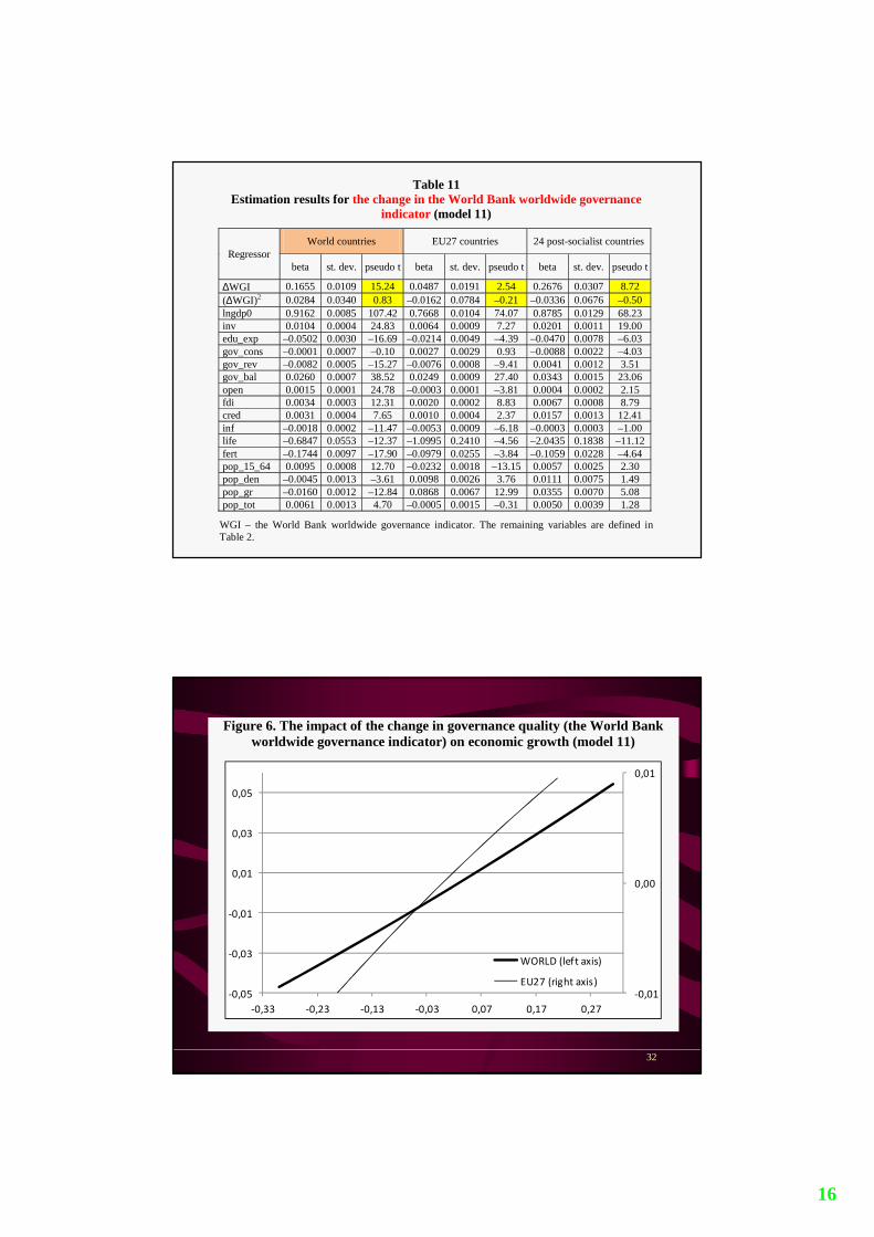
Table 11 Estimation results for the change in the World Bank worldwide governance
indicator (model 11)
Regressor World countries EU27 countries 24 post-socialist countries
beta st. dev. pseudo t beta st. dev. pseudo t beta st. dev. pseudo t
∆WGI 0.1655 0.0109 15.24 0.0487 0.0191 2.54 0.2676 0.0307 8.72 (∆WGI)2 0.0284 0.0340 0.83 –0.0162 0.0784 –0.21 –0.0336 0.0676 –0.50 lngdp0 0.9162 0.0085 107.42 0.7668 0.0104 74.07 0.8785 0.0129 68.23 inv 0.0104 0.0004 24.83 0.0064 0.0009 7.27 0.0201 0.0011 19.00 edu_exp –0.0502 0.0030 –16.69 –0.0214 0.0049 –4.39 –0.0470 0.0078 –6.03 gov_cons –0.0001 0.0007 –0.10 0.0027 0.0029 0.93 –0.0088 0.0022 –4.03 gov_rev –0.0082 0.0005 –15.27 –0.0076 0.0008 –9.41 0.0041 0.0012 3.51 gov_bal 0.0260 0.0007 38.52 0.0249 0.0009 27.40 0.0343 0.0015 23.06 open 0.0015 0.0001 24.78 –0.0003 0.0001 –3.81 0.0004 0.0002 2.15 fdi 0.0034 0.0003 12.31 0.0020 0.0002 8.83 0.0067 0.0008 8.79 cred 0.0031 0.0004 7.65 0.0010 0.0004 2.37 0.0157 0.0013 12.41 inf –0.0018 0.0002 –11.47 –0.0053 0.0009 –6.18 –0.0003 0.0003 –1.00 life –0.6847 0.0553 –12.37 –1.0995 0.2410 –4.56 –2.0435 0.1838 –11.12 fert –0.1744 0.0097 –17.90 –0.0979 0.0255 –3.84 –0.1059 0.0228 –4.64 pop_15_64 0.0095 0.0008 12.70 –0.0232 0.0018 –13.15 0.0057 0.0025 2.30 pop_den –0.0045 0.0013 –3.61 0.0098 0.0026 3.76 0.0111 0.0075 1.49 pop_gr –0.0160 0.0012 –12.84 0.0868 0.0067 12.99 0.0355 0.0070 5.08 pop_tot 0.0061 0.0013 4.70 –0.0005 0.0015 –0.31 0.0050 0.0039 1.28
WGI – the World Bank worldwide governance indicator. The remaining variables are defined in Table 2.
Figure 6. The impact of the change in governance quality (the World Bank worldwide governance indicator) on economic growth (model 11)
-0,01
0,00
0,01
-0,05
-0,03
-0,01
0,01
0,03
0,05
-0,33 -0,23 -0,13 -0,03 0,07 0,17 0,27
WORLD (left axis)
EU27 (right axis)
32

17
INTERPRETATION
• The differences between these models and the earlier onessuggest that the results are not entirely robust to the sample ofcountries and to the exact measure of the regulatory variable.
• Regulatory variables taken from different sources cover variousareas of institutions and they do not exhibit an identical impact oneconomic growth.
• The institutional environment is a very wide economic, politicaland social concept and even considering relatively similar (butsurely not the same) indices measuring regulations we do notobtain the same results.
• This finding will be reinforced later when considering compositeindicators of the aggregated indices, and the democracy index.
33
RESULTS – DEMOCRACY INDEX
• The level of democracy reveals a statistically significant andnonlinear impact on GDP dynamics.
• The direction of this relationship is different in the whole analyzedsample of countries and in the EU27 group.
• The association between the level of democracy and GDPdynamics is rather negative in the whole sample of countries.
34

18
Table 12 Estimation results for the level of the Freedom House democracy index (model
13)
Regressor World countries EU27 countriesa 19 post-socialist countries
beta st. dev. pseudo t beta st. dev. pseudo t beta st. dev. pseudo t
DEM –0.0549 0.0099 –5.56 0.3558 0.0314 11.33 –0.2417 0.0277 –8.72 (DEM)2 0.0049 0.0012 4.13 –0.0251 0.0028 –9.09 0.0313 0.0029 10.74 lngdp0 0.8888 0.0036 247.77 0.8403 0.0070 120.28 0.7997 0.0103 77.99 inv 0.0027 0.0002 11.33 0.0044 0.0004 10.20 0.0105 0.0009 12.10 school_tot –0.0270 0.0020 –13.73 0.0039 0.0012 3.22 0.1441 0.0072 19.89 school_ter –0.0001 0.0003 –0.20 0.0051 0.0005 10.21 0.0109 0.0013 8.13 edu_exp –0.0441 0.0018 –24.18 0.0024 0.0022 1.13 –0.0628 0.0051 –12.26 gov_cons –0.0101 0.0006 –17.40 –0.0191 0.0011 –17.20 –0.0292 0.0018 –16.00 open 0.0009 0.0000 19.71 0.0001 0.0000 2.09 –0.0013 0.0002 –7.94 cab 0.0049 0.0004 13.67 0.0059 0.0004 13.71 0.0086 0.0014 6.38 fdi 0.0061 0.0005 11.46 0.0052 0.0005 11.39 –0.0019 0.0012 –1.61 cred 0.0019 0.0005 4.02 0.0029 0.0004 6.84 0.0093 0.0008 11.42 inf –0.0000 0.0000 –2.68 –0.0015 0.0001 –23.51 –0.0008 0.0001 –14.01 serv –0.0035 0.0003 –11.91 0.0026 0.0003 7.82 0.0025 0.0005 4.64 life 0.6368 0.0204 31.23 0.8363 0.0896 9.34 –0.1246 0.1359 –0.92 fert –0.3132 0.0068 –46.28 –0.1347 0.0128 –10.51 –0.4783 0.0246 –19.41 pop_15_64 0.0164 0.0004 44.61 –0.0010 0.0007 –1.44 –0.0042 0.0026 –1.63 pop_den –0.0118 0.0008 –14.69 –0.0028 0.0014 –2.03 –0.1073 0.0063 –16.98 pop_gr –0.0015 0.0017 –0.90 –0.0243 0.0029 –8.39 –0.0481 0.0071 –6.80 pop_tot –0.0043 0.0007 –6.29 –0.0052 0.0013 –3.96 0.0268 0.0031 8.60
a Without Greece. DEM – the Freedom House democracy index. The remaining variables are defined in Table 2.
Figure 7. The impact of the level of democracy (Freedom House index) on economic growth (model 13)
1,20
1,21
1,22
1,23
1,24
1,25
1,26
1,27
-0,16
-0,15
-0,14
-0,13
-0,12
-0,11
-0,10
-0,09
-0,08
-0,07
1,5 2,5 3,5 4,5 5,5 6,5
WORLD (left axis)
EU27 (right axis)
36

19
Table 13 Estimation results for the change in the Freedom House democracy index
(model 15)
Regressor World countries EU27 countriesa 19 post-socialist countries
beta st. dev. pseudo t beta st. dev. pseudo t beta st. dev. pseudo t
∆DEM –0.0059 0.0018 –3.26 0.0230 0.0031 7.36 –0.0175 0.0064 –2.72 (∆DEM)2 –0.0057 0.0006 –9.44 –0.0150 0.0008 –18.54 –0.0045 0.0015 –3.05 lngdp0 0.8776 0.0046 192.82 0.8241 0.0116 71.07 0.9094 0.0107 85.03 inv 0.0015 0.0003 5.18 0.0028 0.0005 6.03 0.0121 0.0011 10.91 school_tot –0.0136 0.0019 –7.28 0.0090 0.0014 6.67 0.0851 0.0104 8.21 school_ter –0.0001 0.0004 –0.37 0.0085 0.0006 15.08 0.0038 0.0017 2.26 edu_exp –0.0292 0.0021 –13.88 0.0175 0.0024 7.20 –0.0203 0.0058 –3.52 gov_cons –0.0033 0.0005 –6.12 –0.0060 0.0012 –5.17 –0.0198 0.0022 –8.90 open 0.0002 0.0001 4.42 0.0006 0.0001 10.95 –0.0010 0.0002 –5.24 cab 0.0034 0.0004 9.31 0.0082 0.0006 14.80 0.0017 0.0013 1.31 fdi 0.0066 0.0006 10.96 0.0079 0.0005 16.93 –0.0002 0.0015 –0.15 cred 0.0028 0.0005 5.14 0.0022 0.0005 4.50 0.0067 0.0011 5.97 inf –0.0000 0.0000 –2.12 –0.0012 0.0001 –14.07 –0.0006 0.0001 –6.81 serv –0.0040 0.0004 –10.71 0.0031 0.0004 8.71 0.0022 0.0007 3.02 life 0.3435 0.0210 16.36 0.4807 0.1278 3.76 0.1029 0.1461 0.70 fert –0.3617 0.0139 –26.00 –0.0680 0.0083 –8.21 –0.2877 0.0263 –10.93 pop_15_64 0.0037 0.0005 7.14 0.0021 0.0011 1.81 0.0054 0.0030 1.82 pop_den –0.0115 0.0009 –13.04 –0.0054 0.0015 –3.70 –0.0384 0.0060 –6.42 pop_gr 0.0470 0.0025 18.47 –0.0345 0.0031 –11.08 –0.0616 0.0075 –8.17 pop_tot –0.0031 0.0007 –4.32 –0.0087 0.0012 –7.03 0.0102 0.0038 2.65
a Without Greece. DEM – the Freedom House democracy index. The remaining variables are defined in Table 2.
Figure 8. The impact of the change in democracy (Freedom House index) on economic growth (model 15)
-0,04
-0,03
-0,02
-0,01
0,00
0,01
-0,05
-0,04
-0,03
-0,02
-0,01
0,00
0,01
-1,6 -0,6 0,4 1,4 2,4
WORLD (left axis)
EU27 (right axis)
38

20
INTERPRETATION
• At the first view, this relationship may be interpreted as spurious.
• However, the results might confirm that democracy reveals anonlinear impact on economic growth and the fastest-growingcountries are those which are the most and the least democratic.
• E.g. some non-democratic countries (United Arab Emirates orChina) revealed during the last decades very rapid economicgrowth, like several democratic countries (Luxembourg or theUnited States).
• It may be the case that a medium level of democracy is the mostdetrimental to growth.
39
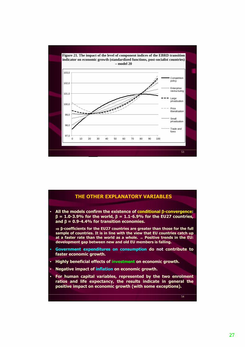
RESULTS – TRANSITION INDICATOR
• The progress in structural (market) reforms shows a positiveimpact on output growth.
• The level of the EBRD transition indicator affects GDP dynamics ina nonlinear way.
40

21
Table 14 Estimation results for the level of and the change in the EBRD transition
indicator (models 19 and 21)
Regressor
Model 19: 27 post-socialist countries
Model 21: 27 post-socialist countries
beta st. dev. pseudo t beta st. dev. pseudo t
TRAN –0.1836 0.0506 –3.63 (TRAN)2 0.0515 0.0092 5.61 ∆TRAN 0.0111 0.0209 0.53 (∆TRAN)2 –0.1237 0.0135 –9.14 lngdp0 0.8851 0.0110 80.68 0.8755 0.0101 86.39 inv 0.0119 0.0007 16.90 0.0172 0.0009 19.83 gov_cons –0.0384 0.0018 –21.36 –0.0272 0.0018 –15.10 open 0.0009 0.0002 5.42 0.0015 0.0002 8.05 pop_15_64 0.0656 0.0014 48.28 0.0641 0.0016 40.16 pop_den –0.1151 0.0039 –29.83 –0.0073 0.0046 –1.58 pop_gr 0.0034 0.0034 1.01 –0.0506 0.0042 –11.94 pop_tot –0.0123 0.0027 –4.48 –0.0048 0.0031 –1.54
TRAN – the EBRD transition indicator. The remaining variables are defined in Table 2.
Figure 9. The impact of the level in the progress of market reforms (the EBRD transition indicator) on economic growth in the post-socialist countries (model
19)
-0,20
-0,15
-0,10
-0,05
0,00
0,05
0,10
1,5 2 2,5 3 3,5 4
42

22
INTERPRETATION
• Transition countries, to accelerate economic growth and to comecloser to Western Europe in terms of the level of development,should undertake market reforms in the areas of privatization,enterprise restructuring, international trade and foreign exchangesystem, price liberalization etc.
• There is much room to carry out such reforms especially in thenon-EU transition countries, namely post-Yugoslav republics(Serbia and Montenegro, Bosnia and Herzegovina, Macedonia) andthe CIS countries (Ukraine, Belarus as well as Caucasian andCentral Asian republics).
43
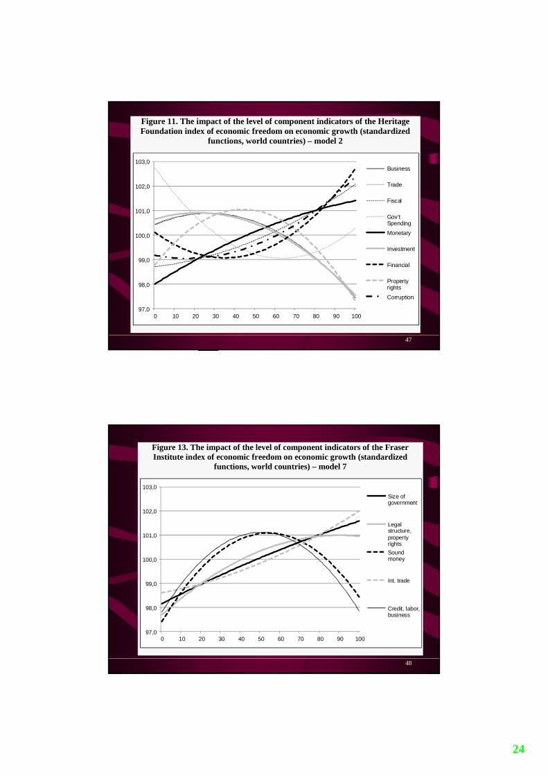
COMPONENT INDICATORS (1/3)
• First, the individual component indicators of the aggregatedregulatory indices sometimes reveal similar behavior as regardsthe impact on economic growth.
• This concerns mainly the component indices of the HeritageFoundation index of economic freedom for which the positiverelationship with economic growth was evidenced in the case ofmost of them.
• Component indices of the EBRD transition indicator (in levels) alsoreveal a positive impact on economic growth.
• Some similar tendencies may also be found for componentindicators of the Fraser Institute index of economic freedom andthe worldwide governance indicator.
44

23
COMPONENT INDICATORS (2/3)
• Second, the similarity of the results is not a rule.
• It may be argued that various areas of regulations affect the paceof economic growth differently, taking into account also thestatistical significance of the impact as well as the character of anonlinear relationship (concave vs. convex functions).
⇒⇒⇒⇒ The results are not robust to a selected institutional variable.
• Cause: indices analyzed in this study cover different regulatoryenvironment; and various institutional areas may exhibit differentimpact on economic growth.
⇒⇒⇒⇒ The need for further testing of the relationship betweenregulations (institutions) and economic growth – also with theuse of non-econometrical approaches.
45
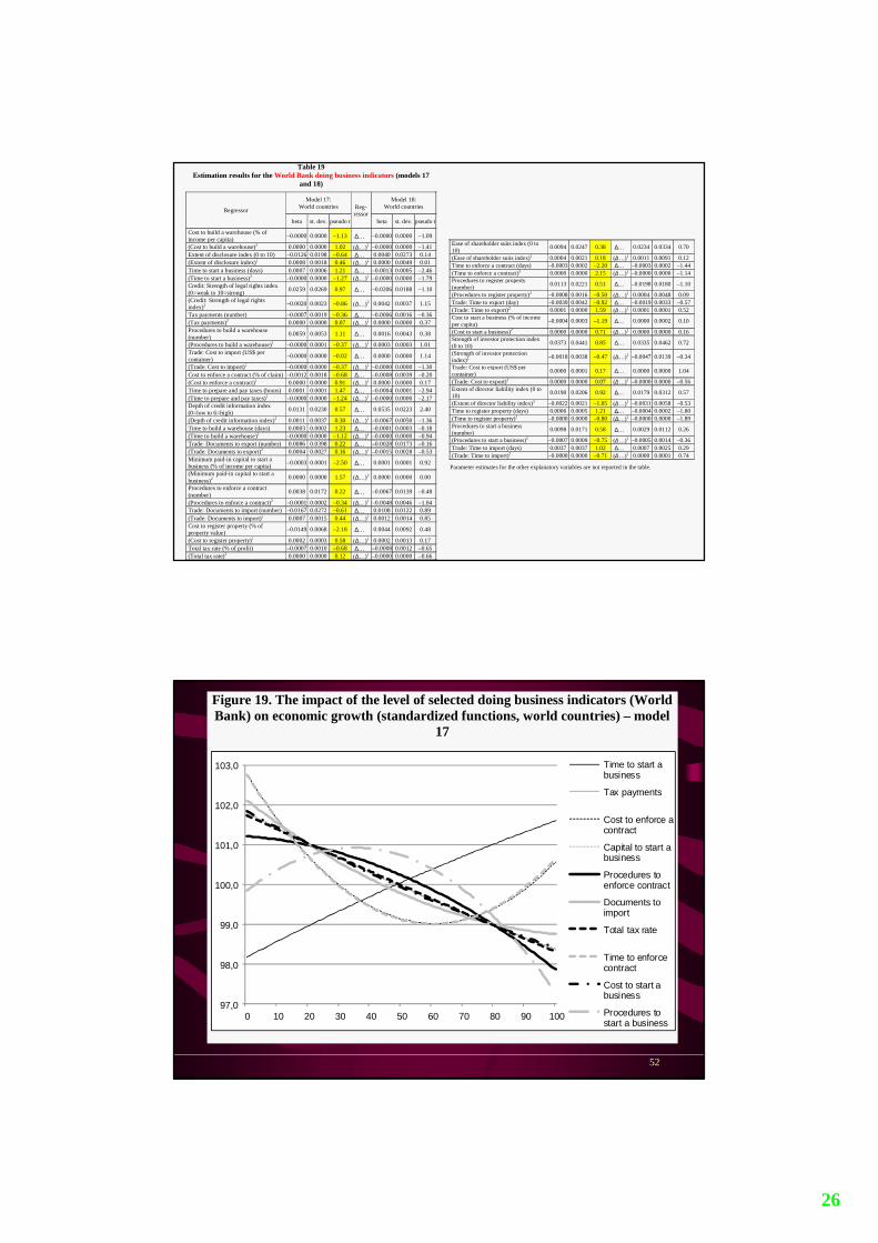
COMPONENT INDICATORS (3/3)
• Almost all the doing business indicators do not reveal astatistically significant association with economic growth.
⇒ The analysis based on panel data with the use of overlappingperiods is better than that based on cross-sectional data in thesense that the former one leads more often to statisticallysignificant results.
⇒ If the whole analysis presented here was carried out based oncross-sectional data, it would be possible to get the majority ofinsignificant results and the conclusions would be very weak.
46
24
Figure 11. The impact of the level of component indicators of the Heritage Foundation index of economic freedom on economic growth (standardized
functions, world countries) – model 2
97,0
98,0
99,0
100,0
101,0
102,0
103,0
0 10 20 30 40 50 60 70 80 90 100
Business
Trade
Fiscal
Gov'tSpending
Monetary
Investment
Financial
Propertyrights
Corruption
47
Figure 13. The impact of the level of component indicators of the Fraser Institute index of economic freedom on economic growth (standardized
functions, world countries) – model 7
97,0
98,0
99,0
100,0
101,0
102,0
103,0
0 10 20 30 40 50 60 70 80 90 100
Size ofgovernment
Legalstructure,propertyrights
Soundmoney
Int. trade
Credit, labor,business
48

25
Figure 15. The impact of the level of component indices of the World Bank worldwide governance indicator on economic growth (standardized functions,
world countries) – model 10
97,0
98,0
99,0
100,0
101,0
102,0
103,0
0 10 20 30 40 50 60 70 80 90 100
Voice &accountability
Politicalstability
Governmenteffectiveness
Regulatoryquality
Rule of law
Corruption
49
Figure 17. The impact of the level of component indicators of the Freedom House democracy index and freedom of the press index on economic growth
(standardized functions, world countries) – model 14
97,0
98,0
99,0
100,0
101,0
102,0
103,0
0 10 20 30 40 50 60 70 80 90 100
Politicalrights
Civilliberties
Freedomof thepress
50
26
Table 19 Estimation results for the World Bank doing business indicators (models 17
and 18)
Regressor
Model 17: World countries Reg-
ressor
Model 18: World countries
beta st. dev. pseudo t beta st. dev. pseudo t
Cost to build a warehouse (% of income per capita)
–0.0000 0.0000 –1.13 ∆… –0.0000 0.0000 –1.09
(Cost to build a warehouse)2 0.0000 0.0000 1.02 (∆…)2 –0.0000 0.0000 –1.41 Extent of disclosure index (0 to 10) –0.0126 0.0198 –0.64 ∆… 0.0040 0.0273 0.14 (Extent of disclosure index)2 0.0008 0.0018 0.46 (∆…)2 0.0000 0.0049 0.01 Time to start a business (days) 0.0007 0.0006 1.21 ∆… –0.0013 0.0005 –2.46 (Time to start a business)2 –0.0000 0.0000 –1.27 (∆…)2 –0.0000 0.0000 –1.79 Credit: Strength of legal rights index (0=weak to 10=strong)
0.0259 0.0269 0.97 ∆… –0.0206 0.0188 –1.10
(Credit: Strength of legal rights index)2
–0.0020 0.0023 –0.86 (∆…)2 0.0042 0.0037 1.15
Tax payments (number) –0.0007 0.0019 –0.36 ∆… –0.0006 0.0016 –0.36 (Tax payments)2 0.0000 0.0000 0.07 (∆…)2 0.0000 0.0000 0.37 Procedures to build a warehouse (number)
0.0059 0.0053 1.11 ∆… 0.0016 0.0043 0.38
(Procedures to build a warehouse)2 –0.0000 0.0001 –0.37 (∆…)2 0.0003 0.0003 1.01 Trade: Cost to import (US$ per container)
–0.0000 0.0000 –0.02 ∆… 0.0000 0.0000 1.14
(Trade: Cost to import)2 –0.0000 0.0000 –0.37 (∆…)2 –0.0000 0.0000 –1.30 Cost to enforce a contract (% of claim) –0.0012 0.0018 –0.68 ∆… –0.0008 0.0039 –0.20 (Cost to enforce a contract)2 0.0000 0.0000 0.91 (∆…)2 0.0000 0.0000 0.17 Time to prepare and pay taxes (hours) 0.0001 0.0001 1.47 ∆… –0.0004 0.0001 –2.94 (Time to prepare and pay taxes)2 –0.0000 0.0000 –1.24 (∆…)2 –0.0000 0.0000 –2.17 Depth of credit information index (0=low to 6=high)
0.0131 0.0230 0.57 ∆… 0.0535 0.0223 2.40
(Depth of credit information index)2 0.0011 0.0037 0.30 (∆…)2 –0.0067 0.0050 –1.36 Time to build a warehouse (days) 0.0003 0.0002 1.23 ∆… –0.0001 0.0003 –0.18 (Time to build a warehouse)2 –0.0000 0.0000 –1.12 (∆…)2 –0.0000 0.0000 –0.94 Trade: Documents to export (number) 0.0086 0.0398 0.22 ∆… –0.0028 0.0173 –0.16 (Trade: Documents to export)2 0.0004 0.0027 0.16 (∆…)2 –0.0015 0.0028 –0.53 Minimum paid-in capital to start a business (% of income per capita)
–0.0003 0.0001 –2.50 ∆… 0.0001 0.0001 0.92
(Minimum paid-in capital to start a business)2
0.0000 0.0000 1.57 (∆…)2 0.0000 0.0000 0.00
Procedures to enforce a contract (number)
0.0038 0.0172 0.22 ∆… –0.0067 0.0139 –0.48
(Procedures to enforce a contract)2 –0.0001 0.0002 –0.34 (∆…)2 –0.0048 0.0046 –1.04 Trade: Documents to import (number) –0.0167 0.0272 –0.61 ∆… 0.0108 0.0122 0.89 (Trade: Documents to import)2 0.0007 0.0015 0.44 (∆…)2 0.0012 0.0014 0.85 Cost to register property (% of property value)
–0.0149 0.0068 –2.18 ∆… 0.0044 0.0092 0.48
(Cost to register property)2 0.0002 0.0003 0.58 (∆…)2 0.0002 0.0013 0.17 Total tax rate (% of profit) –0.0007 0.0010 –0.68 ∆… –0.0008 0.0012 –0.65 (Total tax rate)2 0.0000 0.0000 0.12 (∆…)2 –0.0000 0.0000 –0.66
Ease of shareholder suits index (0 to 10)
0.0094 0.0247 0.38 ∆… 0.0234 0.0334 0.70
(Ease of shareholder suits index)2 0.0004 0.0021 0.18 (∆…)2 0.0011 0.0091 0.12 Time to enforce a contract (days) –0.0003 0.0002 –2.20 ∆… –0.0003 0.0002 –1.44 (Time to enforce a contract)2 0.0000 0.0000 2.15 (∆…)2 –0.0000 0.0000 –1.14 Procedures to register property (number)
0.0113 0.0221 0.51 ∆… –0.0198 0.0180 –1.10
(Procedures to register property)2 –0.0008 0.0016 –0.50 (∆…)2 0.0004 0.0048 0.09 Trade: Time to export (day) –0.0039 0.0042 –0.92 ∆… –0.0019 0.0033 –0.57 (Trade: Time to export)2 0.0001 0.0000 1.59 (∆…)2 0.0001 0.0001 0.52 Cost to start a business (% of income per capita)
–0.0004 0.0003 –1.19 ∆… 0.0000 0.0002 0.10
(Cost to start a business)2 0.0000 0.0000 0.71 (∆…)2 0.0000 0.0000 0.16 Strength of investor protection index (0 to 10)
0.0373 0.0441 0.85 ∆… 0.0335 0.0462 0.72
(Strength of investor protection index)2
–0.0018 0.0038 –0.47 (∆…)2 –0.0047 0.0139 –0.34
Trade: Cost to export (US$ per container)
0.0000 0.0001 0.17 ∆… 0.0000 0.0000 1.04
(Trade: Cost to export)2 0.0000 0.0000 0.07 (∆…)2 –0.0000 0.0000 –0.56 Extent of director liability index (0 to 10)
0.0190 0.0206 0.92 ∆… 0.0179 0.0312 0.57
(Extent of director liability index)2 –0.0022 0.0021 –1.05 (∆…)2 –0.0031 0.0058 –0.53 Time to register property (days) 0.0006 0.0005 1.21 ∆… –0.0004 0.0002 –1.80 (Time to register property)2 –0.0000 0.0000 –0.80 (∆…)2 –0.0000 0.0000 –1.89 Procedures to start a business (number)
0.0098 0.0171 0.58 ∆… 0.0029 0.0112 0.26
(Procedures to start a business)2 –0.0007 0.0009 –0.75 (∆…)2 –0.0005 0.0014 –0.36 Trade: Time to import (days) 0.0037 0.0037 1.02 ∆… 0.0007 0.0025 0.29 (Trade: Time to import)2 –0.0000 0.0000 –0.71 (∆…)2 0.0000 0.0001 0.74
Parameter estimates for the other explanatory variables are not reported in the table.
Figure 19. The impact of the level of selected doing business indicators (World Bank) on economic growth (standardized functions, world countries) – model
17
97,0
98,0
99,0
100,0
101,0
102,0
103,0
0 10 20 30 40 50 60 70 80 90 100
Time to start abusiness
Tax payments
Cost to enforce acontract
Capital to start abusiness
Procedures toenforce contract
Documents toimport
Total tax rate
Time to enforcecontract
Cost to start abusiness
Procedures tostart a business
52
27
Figure 21. The impact of the level of component indices of the EBRD transition indicator on economic growth (standardized functions, post-socialist countries)
– model 20
97,0
98,0
99,0
100,0
101,0
102,0
103,0
0 10 20 30 40 50 60 70 80 90 100
Competitionpolicy
Enterpriserestructuring
Largeprivatisation
Priceliberalisation
Smallprivatisation
Trade andforex
53
54
THE OTHER EXPLANATORY VARIABLES
• All the models confirm the existence of conditional ββββ-convergence:ββββ = 1.0-3.9% for the world, ββββ = 1.1-6.9% for the EU27 countries,and ββββ = 0.9-4.4% for transition economies.
⇒⇒⇒⇒ ββββ-coefficients for the EU27 countries are greater than those for the fullsample of countries. It is in line with the view that EU countries catch upat a faster rate than the world as a whole. →→→→ Positive trends in the EU:development gap between new and old EU members is falling.
• Government expenditures on consumption do not contribute tofaster economic growth.
• Highly beneficial effects of investment on economic growth.
• Negative impact of inflation on economic growth.
• For human capital variables, represented by the two enrolmentratios and life expectancy, the results indicate in general thepositive impact on economic growth (with some exceptions).

28
55
SUMMARY AND MAIN FINDINGS
1. The study examines the relationship between the regulatory variables and economicgrowth on the basis of Bayesian model pooling applied to Blundell and Bond’s GMMsystem estimator.
2. The areas of regulations (institutions) are measured by the following indicators: index ofeconomic freedom, worldwide governance indicators, democracy index, doing businessindicators, transition indicators.
3. Most of the models are estimated based on overlapping panel data and they includenonlinearities.
4. In general, regulatory environment is an important determinant of economic growth.
5. To achieve rapid growth, it is necessary to increase economic freedom, quality ofgovernance, and market reforms.
6. The association between regulatory variables and GDP dynamics is mostly nonlinear.
7. The countries with greater scope of economic freedom record more rapid GDP growth buta given increase in economic freedom has a higher impact on growth in those countriesthat are economically not (or partly) free.
8. However, the results are not robust in a lot of areas – with regard to the sample ofcountries, the exact measure of the regulatory variable, and the type of nonlinear impact(concave vs. convex functions).
9. There are many factors affecting both regulations and GDP dynamics as well as manytransmission channels between these areas and the results sometimes are mixed.
56
Thank youfor the attention ☺☺☺☺