insurance regulation and policy firesales

Insurance Regulation and Policy Firesales∗

Ralph S. J. Koijen† Motohiro Yogo‡

March 30, 2012

Abstract

During the financial crisis, life insurers sold long-term insurance policies at firesale

prices. In January 2009, the average markup, relative to actuarial value, was −25

percent for 30-year term annuities as well as life annuities and −52 percent for universal

life insurance. This extraordinary pricing behavior was a consequence of statutory

reserve regulation that allowed life insurers to record far less than a dollar of reserves per

dollar of future insurance liability. Using exogenous variation in reserve requirements

across different types of policies, we identify the shadow cost of financial constraints

for life insurers. The shadow cost of raising a dollar of excess reserves was nearly $5

for the average insurance company in January 2009.

JEL classification: G22, G28

Keywords: Annuities, Financial frictions, Leverage, Life insurance, Regulation, Statutory

reserves

∗For comments and discussions, we thank Sam Schulhofer-Wohl and seminar participants at FederalReserve Bank of Minneapolis and University of Minnesota. We thank Jahiz Barlas, Minsoo Kim, PeterNebres, and Julia Pei for research assistance. A.M. Best Company, Annuity Shopper, and COMPULIFESoftware own the copyright to their respective data, which we use in this paper with permission. Theviews expressed herein are those of the authors and not necessarily those of the Federal Reserve Bank ofMinneapolis, the Federal Reserve System, or the National Bureau of Economic Research.

†University of Chicago, National Bureau of Economic Research, and Netspar-Tilburg University (e-mail:[email protected])

‡Federal Reserve Bank of Minneapolis (e-mail: [email protected])

1. Introduction

The traditional view of insurance markets is that insurance companies operate in a perfect

capital market that allows them to produce insurance at nearly constant marginal cost.

Consequently, the equilibrium price is determined by the demand side of the market, either

by life-cycle demand (Yaari, 1965) or informational frictions (Rothschild and Stiglitz, 1976).

Contrary to this traditional view, this paper shows that insurance companies are financial

institutions whose pricing behavior can be profoundly affected by financial constraints and

the regulation of statutory reserves.

Our key finding is that life insurers sold long-term insurance policies at firesale prices

during a period of few months around January 2009. The average markup, relative to

actuarial value (i.e., the present discounted value of future policy claims), was −25 percent

for 30-year term annuities as well as life annuities at age 50. Similarly, the average markup

was −52 percent for universal life insurance at age 30. These deep discounts are in sharp

contrast to the 6 to 10 percent markup that life insurers earn in ordinary times (Mitchell et al.,

1999). In the cross section of insurance policies, the discounts were deeper for those policies

with looser statutory reserve requirements. In the cross section of insurance companies, the

discounts were deeper for those companies whose balance sheets were most adversely affected

prior to January 2009.

This extraordinary pricing behavior was due to a remarkable coincidence of two circum-

stances. First, the financial crisis had an adverse impact on insurance companies’ balance

sheets. Insurance companies had to quickly recapitalize in order to control their leverage

ratio and to prevent a rating downgrade or regulatory action. Second, the regulation gov-

erning statutory reserves in the United States allowed life insurers to record far less than

a dollar of reserves per dollar of future insurance liability during a period of few months

around January 2009. Therefore, insurance companies were able to reduce their leverage

ratio by selling insurance policies at a price far below actuarial value, as long as that price

was above the reserve value.

2

We formalize our hypothesis in a structural model of insurance pricing that is otherwise

standard, except for a leverage constraint that is familiar from macroeconomics and finance

(e.g., Kiyotaki and Moore, 1997; Brunnermeier and Pedersen, 2009). The insurance company

sets prices for various types of policies to maximize profits, subject to a leverage constraint

that the ratio of statutory reserves to assets cannot exceed a targeted value. Whenever

the leverage constraint binds, the insurance company optimally prices a policy below its

actuarial value if the transaction has a negative marginal impact on leverage. The Lagrange

multiplier on the leverage constraint has a structural interpretation as the shadow cost of

raising a dollar of excess reserves.

To test our hypothesis, we construct a panel dataset of nearly 35,000 observations on

insurance prices from January 1989 through July 2011. Our data cover term annuities,

life annuities, and universal life insurance for both males and females as well as various

age groups. Because statutory reserve regulation implies different reserve requirements for

different types of policies, we exploit that exogenous variation to identify the shadow cost

of financial constraints, which has remained elusive in the previous literature. We find that

the shadow cost of the leverage constraint is essentially zero for most of the sample, except

around January 2001 and in January 2009. We find that the shadow cost of raising a dollar

of excess reserves was nearly $5 for the average insurance company in January 2009. This

cost varies from $1 to $13 per dollar of excess reserves for the cross section of insurance

companies in our sample.

From an investor’s perspective, January 2009 was an especially attractive opportunity

to be in the market for insurance policies. For example, a 30-year term annuity could have

been purchased for 25 percent less than a portfolio of Treasury bonds with identical cash

flows. While solvency might have been a concern for some insurance companies, insurance

policies are ultimately backed by the state guarantee fund (e.g., up to $250k for annuities

and $300k for life insurance in California). Therefore, the only scenario in which an investor

would not be repaid is if all insurance companies associated with the state guarantee fund

3

were to systemically fail.

From an insurance company’s perspective, it is less obvious why it was optimal to discount

insurance policies in January 2009. A potential explanation is that insurance companies

anticipated some chance of default, so that their expected liability was less than the full face

value of insurance policies. Unfortunately, this explanation is inconsistent with the evidence

during the Great Depression. Warshawsky (1988) finds that annuity prices closely track the

actuarial value, based on the 20-year Treasury yield, throughout the Great Depression. In

particular, insurance companies did not sell annuities at firesale prices in 1932 when corporate

default spreads were much higher than the heights reached during the recent financial crisis.

Overall, the evidence is more consistent with our explanation based on financial constraints

and statutory reserve regulation.

The remainder of the paper is organized as follows. Section 2 describes our data and

documents key facts that motive our study of insurance prices. Section 3 reviews key features

of statutory reserve regulation that are relevant for our analysis. In Section 4, we develop

a structural model of insurance pricing subject to a leverage constraint, which shows how

statutory reserve regulation can affect insurance prices. In Section 5, we use our structural

model of insurance pricing to estimate the shadow cost of the leverage constraint. Section 6

concludes.

2. Annuity and Life Insurance Prices

2.1 Data Construction

2.1.1 Annuity Prices

Our annuity prices are from the Annuity Shopper (Stern, 2011), which is a semiannual

publication (every January and July) of annuity price quotes from the leading life insurers.

Following Mitchell et al. (1999), we focus on annuities that are single premium, immediate,

4

and non-qualified. This means that the premium is paid upfront as a single lump sum,

that the income payments start immediately after the premium payment, and that only the

interest portion of the payments is taxable. Our data consist of three types of policies: term

annuities, life annuities, and guaranteed annuities. For term annuities, we have quotes for

5- through 30-year maturities (every 5 years in between). For life and guaranteed annuities,

we have quotes for males and females between ages 50 and 90 (every 5 years in between).

A term annuity is a policy with annual income payments for a fixed term of M years. Let

Rt(m) be the zero-coupon Treasury yield at maturity m in month t. We define the actuarial

value of an M-year term annuity per dollar of income as

Vt(M) =

M∑m=1

1

Rt(m)m. (1)

A life annuity is a policy with annual income payments until death of the insured. Let

pn be the one-year survival probability at age n, and let N be the maximum attainable age

according to the appropriate mortality table. We define the actuarial value of a life annuity

at age n per dollar income as

Vt(n) =N−n∑m=1

∏m−1l=0 pn+l

Rt(m)m. (2)

A guaranteed annuity is a variant of the life annuity whose income payments are guaran-

teed to continue for the first M years, even if the insured dies during that period. We define

the actuarial value of an M-year guaranteed annuity at age n per dollar of income as

Vt(n,M) =M∑

m=1

1

Rt(m)m+

N−n∑m=M+1

∏m−1l=0 pn+l

Rt(m)m. (3)

We calculate the actuarial value for each type of policy at each date using the zero-coupon

Treasury yield curve (Gurkaynak, Sack, and Wright, 2007) and the appropriate mortality

table from the Society of Actuaries. We use the 1983 Annuity Mortality Basic Table prior to

5

December 2000, and the 2000 Annuity Mortality Basic Table since December 2000. These

mortality tables are derived from the actual mortality experience of insured pools, based on

data provided by various insurance companies. Therefore, they account for adverse selection

in annuity markets, that is, an insured pool of annuitants has higher life expectancy than

the overall population. We smooth the transition between the two versions of the mortality

tables by geometrically averaging.

2.1.2 Life Insurance Prices

Our life insurance prices are from COMPULIFE Software, which is a computer-based quota-

tion system for insurance brokers. We focus on guaranteed universal life policies, which are

quoted for the leading life insurers since January 2005. These policies have constant guar-

anteed premiums and accumulate no cash value, so they are essentially “permanent” term

life policies.1 We pull quotes for the regular health category at the face amount of $250,000

in the sate of California. COMPULIFE recommended California for our study because it is

the most populous state with a wide representation of insurance companies. We focus on

males and females between ages 30 and 90 (every 10 years in between).

Universal life insurance is a policy that pays out a death benefit upon death of the insured.

The policy is in effect as long as the policyholder makes an annual premium payment while

the insured is alive. We define the actuarial value of universal life insurance at age n per

dollar of death benefit as

Vt(n) =

(1 +

N−n−1∑m=1

∏m−1l=0 pn+l

Rt(m)m

)−1(N−n∑m=1

∏m−2l=0 pn+l(1− pn+m−1)

Rt(m)m

). (4)

Note that this formula does not take into account the potential lapsation of policies, that is,

the policyholder may drop coverage prior to the death of the insured. There is currently no

1While COMPULIFE has quotes for various types of policies from annual renewable to 30-year term lifepolicies, they are not useful for our purposes. This is because a term life policy typically has a renewal optionat the end of the guaranteed term. Because the premiums under the renewal option vary significantly acrossinsurance companies, cross-sectional price comparisons are difficult and imprecise.

6

agreed upon standard for lapsation pricing, partly because lapsations are difficult to model

and predict. While some insurance companies price in low levels of lapsation, others take

the conservative approach of assuming no lapsation in life insurance valuation.

We calculate the actuarial value for each type of policy at each date using the zero-coupon

Treasury yield curve and the appropriate mortality table from the Society of Actuaries. We

use the 2001 Valuation Basic Table prior to December 2008, and the 2008 Valuation Basic

Table since December 2008. These mortality tables are derived from the actual mortality

experience of insured pools, based on data provided by various insurance companies. There-

fore, they account for adverse selection in life insurance markets. We smooth the transition

between the two versions of the mortality tables by geometrically averaging.

2.1.3 Insurance Companies’ Balance Sheets

We obtain balance sheet data and A.M. Best ratings for insurance companies through the

Best’s Insurance Reports CD-ROM for fiscal years 1992 through 2010. We merge annuity

and life insurance prices to the A.M. Best data through company name. The insurance price

observed in January and July of each calender year is matched to the balance sheet data for

the previous fiscal year (i.e., as of December of the previous calendar year).

2.2 Summary Statistics

We start with a broad overview of the industry that we study. Figure 1 reports the an-

nual premiums paid for individual annuities and life insurance, summed across all insurance

companies in the United States with an A.M. Best rating. In the early 1990’s, insurance

companies collected nearly $100 billion in annual premiums for individual life insurance and

about $50 billion for individual annuities. More recently, the annuity market expanded to

$383 billion in 2008. The financial crisis had an adverse effect on annuity demand in 2009,

which subsequently bounced back in 2010.

Table 1 summarizes our data on annuity and life insurance prices. We have 988 ob-

7

servations on 10-year term annuities across 98 insurance companies, covering January 1989

through July 2011. The average markup, defined as the percentage deviation of the quoted

price from actuarial value, is 6.9 percent. Given that term annuities provide a fixed income

stream that an investor can also achieve with Treasury bonds, it is curious why the average

markup is so high. There is considerable cross-sectional variation in pricing across insurance

companies, as indicated by a standard deviation of 5.9 percent (Mitchell et al., 1999).

We have 11,879 observations on life annuities across 106 insurance companies, covering

January 1989 through July 2011. The average markup is 9.8 percent with a standard de-

viation of 8.2 percent. Our data on guaranteed annuities start in July 1989. For 10-year

guaranteed annuities, the average markup is 5.5 percent with a standard deviation of 6.1

percent. For 20-year guaranteed annuities, the average markup is 4.2 percent with a standard

deviation of 4.8 percent.

We have 3,989 observations on universal life insurance across 52 companies, covering

January 2005 through July 2011. The average markup is −4.2 percent with a standard

deviation of 17.9 percent. The negative average markup does not mean that insurance

companies systematically lose money on these policies. With a constant premium and a rising

mortality rate, policyholders are essentially prepaying for coverage later in life. Whenever

a universal life policy is lapsed, the insurance company earns a windfall profit because the

present value of remaining premium payments is typically less than the present value of

the future death benefit. Since there is currently no agreed upon standard for lapsation

pricing, our calculation of actuarial value does not take lapsation into account. We are not

especially concerned that the average markup might be slightly mismeasured because our

focus is mostly on the variation in markups over time and across different types of polices.

2.3 Firesales of Insurance Policies

Figure 2 reports the time series of average markup on term annuities at various maturities,

averaged across insurance companies and reported with a 95 percent confidence interval.

8

The average markup varies between 0 and 10 percent, with the exception of a period of few

months around January 2009. If insurance companies were to change prices on term annuities

to perfectly offset interest rate movements, then the markup would be constant over time.

Hence, variation in the average markup imply that insurance companies do not necessarily

change prices to offset interest rate movements (Charupat, Kamstra, and Milevsky, 2012).

For 30-year term annuities, the average markup fell to an extraordinary −25 percent in

January 2009. This large negative markup was due to insurance companies actively cutting

prices when the historically low Treasury yields implied high actuarial value for these policies.

In January 2009, there is a monotonic relation between the maturity of the policy and the

magnitude of the average markup. Average markup was −16 percent for 20-year, −8 percent

for 10-year, and −3 percent for 5-year term annuities. Excluding the extraordinary period

around January 2009, average markup was negative for 20- and 30-year term annuities only

twice before in our sample, in January 2001 and July 2002.

Figure 3 reports the time series of average markup on life annuities at different ages.

We find a similar phenomenon to that for term annuities. For life annuities at age 50, the

average markup fell to an extraordinary −25 percent in January 2009. There is a monotonic

relation between age, which is negatively related to the effective maturity of the policy, and

the magnitude of the average markup. Average markup was −19 percent at age 60, −11

percent at age 70, and −3 percent at age 80.

Figure 4 reports the time series of average markup on universal life insurance at different

ages. We again find a similar phenomenon to that for term and life annuities. For universal

life insurance at age 30, the average markup fell to an extraordinary −52 in January 2009.

There is a monotonic relation between age and the magnitude of the average markup. Av-

erage markup was −47 percent at age 40, −42 percent at age 50, and −29 percent at age

60.

A potential explanation for the negative markup in January 2009 is that insurance com-

panies anticipated some chance of default, so that their expected liability was less than the

9

full face value of insurance policies. Therefore, their cost of capital was the Baa corporate

bond yield, for example, instead of the Treasury yield. Unfortunately, this explanation does

not work for three reasons. First, if the Baa corporate bond yield were used to calculate

the actuarial value, it would imply that insurance companies earn incredibly high markups

in ordinary times (Mitchell et al., 1999). Second, the firesale of insurance policies was very

short-lived around January 2009, while the corporate default spread remained elevated for

much longer. Third, and perhaps most convincingly, this explanation is inconsistent with

the evidence during the Great Depression as we discussed in the introduction. We now turn

to an alternative explanation based on financial constraints and statutory reserve regulation,

which is more consistent with the evidence.

3. Statutory Reserve Regulation for Life Insurers

When an insurance company sells an annuity or life insurance policy, its assets increase by

the purchase price of the policy. At the same time, the insurance company must record

reserves on the liability side of its balance sheet to cover future policy claims. In the United

States, the amount of statutory reserves that are required for each type of policy is governed

by state law, but all states essentially follow recommended guidelines known as Standard

Valuation Law (National Association of Insurance Commissioners, 2011, Appendix A-820).

Standard Valuation Law establishes discount rates and mortality tables that are to be used

for reserve valuation.

In this section, we review the reserve valuation rules for annuities and life insurance.

Because these policies essentially have zero market beta, finance theory implies that the

economic value of these policies is determined by the term structure of riskless interest

rates. However, Standard Valuation Law requires that the reserve value of these policies be

calculated using a mechanical discount rate that is proportional to the Moody’s composite

yield on seasoned corporate bonds. Insurance companies care about the reserve value of

10

policies insofar as it is used by regulators and rating agencies to determine the adequacy

of statutory reserves. For example, a state regulator may force liquidation of an insurance

company whose assets are insufficient relative to its statutory reserves. Or a rating agency

may downgrade an insurance company whose asset value has fallen relative to its statutory

reserves (A.M. Best Company, Inc., 2011, p. 31).

3.1 Term Annuities

Let yt be the 12-month moving average of the Moody’s composite yield on seasoned corporate

bonds, over the period ending on June 30 of the issuance year of the policy. Standard

Valuation Law specifies the following discount rate for reserve valuation of annuities:

Rt − 1 = 0.03 + 0.8(yt − 0.03), (5)

which is rounded to the nearest 25 basis point. This a constant discount rate that is to be

applied to all expected future cash flows, regardless of maturity. The exogenous variation

in statutory reserve requirements that this mechanical rule generates, both over time and

across different types of policies, allows us to identify the shadow cost of financial constraints

for life insurers.

Figure 5 reports the time series of the discount rate for annuities, together with the

10-year zero-coupon Treasury yield. The discount rate for annuities has generally declined

over the last 20 years as nominal interest rates have fallen. However, the discount rate

for annuities has declined more slowly than the 10-year Treasury yield. This means that

statutory reserve requirements for annuities have become looser over time because a high

discount rate implies low reserve valuation.

The reserve value of an M-year term annuity per dollar of income is

Vt(M) =

M∑m=1

1

Rmt

. (6)

11

Figure 6 reports the ratio of reserve to actuarial value for term annuities (i.e., Vt(M)/Vt(M))

at maturities of 5 to 30 years. Whenever this ratio is equal to one, the insurance company

records a dollar of reserves per dollar of future policy claims in present value. Whenever this

ratio is greater than one, the reserve valuation is conservative in the sense that the insurance

company records reserves that are greater than the present value of future policy claims.

Conversely, whenever this ratio is less than one, the reserve valuation is aggressive in the

sense that the insurance company records reserves that are less than the present value of

future policy claims.

For the 30-year term annuity, the ratio reaches a peak of 1.20 in November 1994 and a

trough of 0.73 in January 2009. If the insurance company were to sell a 30-year term annuity

at actuarial value in November 1994, its reserves would increase by $1.20 per dollar of policies

sold. This implies a loss of $0.20 in capital surplus funds (i.e., total admitted assets minus

total liabilities) per dollar of policies sold. In contrast, if the insurance company were to sell

a 30-year term annuity at actuarial value in January 2009, its reserves would only increase

by $0.73 per dollar of policies sold. This implies a gain of $0.27 in capital surplus funds per

dollar of policies sold.

3.2 Life Annuities

The reserve valuation of life annuities requires mortality tables. The Society of Actuaries

produces two versions of mortality tables, which are called basic and loaded. The loaded

tables, which are used for reserve valuation, are conservative versions of the basic tables that

underestimate the mortality rates. The loaded tables ensure that insurance companies have

adequate reserves, even if actual mortality rates turn out to be lower than those projected

by the basic tables. For calculating the reserve value, we use the 1983 Annuity Mortality

Table prior to December 2000, and the 2000 Annuity Mortality Table since December 2000.

Let pn be the one-year survival probability at age n, and let N be the maximum attainable

age according to the appropriate loaded mortality table. The reserve value of a life annuity

12

at age n per dollar of income is

Vt(n) =N−n∑m=1

∏m−1l=0 pn+l

Rmt

, (7)

where the discount rate is given by equation (5). Similarly, the reserve value of an M-year

guaranteed annuity at age n per dollar of income is

Vt(n,M) =M∑

m=1

1

Rmt

+N−n∑

m=M+1

∏m−1l=0 pn+l

Rmt

. (8)

Figure 6 reports the ratio of reserve to actuarial value for life annuities, 10-year guaranteed

annuities, and 20-year guaranteed annuities for males aged 50 to 80 (every 10 years in

between). For these life annuities, the time-series variation in the ratio of reserve to actuarial

value is quite similar to that for term annuities. In particular, the ratio reaches a peak in

November 1994 and a trough in January 2009. Since the reserve valuation of term annuities

depends only on the discount rates, the similarity with term annuities implies that discount

rates, rather than mortality tables, have a predominant effect on the reserve valuation of life

annuities.

3.3 Life Insurance

Let yt be the minimum of the 12-month and the 36-month moving average of the Moody’s

composite yield on seasoned corporate bonds, over the period ending on June 30 of the year

prior to issuance of the policy. Standard Valuation Law specifies the following discount rate

for reserve valuation of life insurance:

Rt(M)− 1 = 0.03 + w(M)(min{yt, 0.09} − 0.03) + 0.5w(M)(max{yt, 0.09} − 0.09), (9)

13

which is rounded to the nearest 25 basis point. The weighting function for a policy with a

term of M years is

w(M) =

⎧⎪⎪⎪⎪⎨⎪⎪⎪⎪⎩0.50 if M ≤ 10

0.45 if 10 < M ≤ 20

0.35 if M > 20

. (10)

As with life annuities, the American Society of Actuaries produces basic and loaded

mortality tables for life insurance. The loaded tables, which are used for reserve valuation,

are conservative versions of the basic tables that overestimate the mortality rates. The loaded

tables ensure that insurance companies have adequate reserves, even if actual mortality rates

turn out to be higher than those projected by the basic tables. For calculating the reserve

value, we use the 2001 Commissioners Standard Ordinary Mortality Table. The reserve value

of life insurance at age n per dollar of death benefit is

Vt(n) =

(1 +

N−n−1∑m=1

∏m−1l=0 pn+l

Rt(N − n)m

)−1(N−n∑m=1

∏m−2l=0 pn+l(1− pn+m−1)

Rt(N − n)m

). (11)

Figure 7 reports the ratio of reserve to actuarial value for universal life insurance for

males aged 30 to 60 (every 10 years in between). In a period of few months around January

2009, the reserve value falls significantly relative to actuarial value. As shown in Figure 5,

this is caused by the fact that the discount rate for life insurance stays constant during this

period, while the 10-year Treasury yield falls significantly. If an insurance company were to

sell universal life insurance to a 30-year old male in January 2009, its reserves would only

increase by $0.87 per dollar of policies sold. This implies a gain of $0.13 in capital surplus

funds per dollar of policies sold.

14

4. Insurance Pricing under Statutory Reserve Regula-

tion

We now develop a simple model to show how financial constraints and statutory reserve

regulation can affect insurance prices.

4.1 An Insurance Company’s Profit Maximization Problem

An insurance company sells I different types of annuity and life insurance policies, which

we index as i = 1, . . . , I. These policies are differentiated not only by term, but also by sex

and age of the insured. The insurance company faces a downward-sloping demand curve

Qi(P ) for each policy i, where Q′i(P ) < 0. There are various micro-foundations that give

rise to such a demand curve. For example, such a demand curve can be motivated as an

industry equilibrium subject to search frictions (Hortacsu and Syverson, 2004). We will

simply take the demand curve as exogenously given because the precise micro-foundations

are not essential for our purposes.

Let Vi be the actuarial value of policy i. The insurance company chooses the price Pi for

each type of policy to maximize profits:

Π =

I∑i=1

(Pi − Vi)Qi(Pi). (12)

A simple way to interpret this profit function is that for each type of policy that the insurance

company sells for Pi, it can pay Vi to buy a portfolio of zero-coupon Treasury bonds that

replicate the expected future policy claims. For term annuities, this interpretation is exact

in the sense that there is no uncertainty regarding future policy claims. For life annuities

and life insurance, we assume that the insured pools are sufficiently large for the law of large

numbers to apply.

We now describe how the sale of new policies affects the insurance company’s balance

15

sheet. Let A− be its assets prior to the sale of new policies (but after external sources of

financing such as capital injection from the holding company). Its assets after the sale of

new policies is

A = A− +

I∑i=1

PiQi(Pi). (13)

As explained in Section 3, the insurance company must also record reserves on the liability

side of its balance sheet. Let Vi be the reserve value of policy i. Let L− be its statutory

reserves prior to the sale of new policies. Its statutory reserves after the sale of new policies

is

L = L− +I∑

i=1

ViQi(Pi). (14)

The insurance company faces a leverage constraint on the value of its statutory reserves

relative to its assets. Consequently, the insurance company maximizes its profits subject to

the constraint that

L

A≤ φ, (15)

where φ ≤ 1 is the maximum leverage ratio. The underlying assumption is that exceeding

the maximum leverage ratio leads to bad consequences, such as forced liquidation by state

regulators or a rating downgrade.

16

4.2 Optimal Insurance Pricing

Let λ ≥ 0 be the Lagrange multiplier on the leverage constraint (15). The Lagrangian for

the insurance company’s maximization problem is

L =Π+ λ(φA− L

)=

I∑i=1

(Pi − Vi)Qi(Pi) + λ

[φ

(A− +

I∑i=1

PiQi(Pi)

)−(L− +

I∑i=1

ViQi(Pi)

)]. (16)

The first-order condition for each policy i is

∂L∂Pi

=∂Π

∂Pi

+ λ∂(φA− L

)∂Pi

=Qi(Pi) + (Pi − Vi)Q′i(Pi) + λ

[φQi(Pi) +

(φPi − Vi

)Q′

i(Pi)]

=0. (17)

Rearranging equation (17), the price of policy i is

Pi = Vi

(1− 1

εi

)−1(1 + λVi/Vi

1 + λφ

), (18)

where

εi = −PiQ′i(Pi)

Qi(Pi)> 1 (19)

is the elasticity of demand. Moreover, the Lagrange multiplier is

λ = − ∂Π

∂(φA− L

) . (20)

Note that φA− L can be interpreted as the excess reserves of the insurance company. Hence,

the Lagrange multiplier measures the dollar losses that the insurance company is willing to

17

take in order to increase its excess reserves by a dollar.

Suppose the leverage constraint does not bind (i.e., λ = 0). Then the price of policy i is

Pi = Vi

(1− 1

εi

)−1

. (21)

This is the standard Bertrand price of the policy, which is equal to marginal cost plus a

markup that arises from imperfect competition. Now suppose that the leverage constraint

binds (i.e., λ > 0). Then the price of policy i is

Pi ≷ Vi

(1− 1

εi

)−1

ifVi

Vi≷ φ. (22)

When the leverage constraint binds, the price of the policy is higher than the Bertrand

price if issuing the policy tightens the leverage constraint on the margin. Conversely, the

price of the policy is lower than the Bertrand price if issuing the policy relaxes the leverage

constraint.

When the leverage constraint binds, equation (18) and the leverage constraint (i.e., φA =

L) forms a system of I + 1 equations in I + 1 unknowns (i.e., Pi for each policy i = 1, . . . , I

and λ). Solving this system of equations for the Lagrange multiplier,

λ =1

φ

⎛⎝∑i

(φVi(1− 1/εi)

−1 − Vi

)Qi − L− + φA−

L− − φA− −∑i Vi(εi − 1)−1Qi

⎞⎠ . (23)

To understand the intuition for this expression, consider the limiting case of perfectly elastic

demand. The limit as εi → ∞ for all policies is

λ → 1

φ

⎛⎝∑i

(φVi − Vi

)Qi

L− − φA−− 1

⎞⎠ . (24)

This expression shows that the Lagrange multiplier depends on the product of two terms.

The first term says that the Lagrange multiplier is inversely related to the targeted leverage

18

ratio. The second term says that the Lagrange multiplier is proportional to the marginal

increase in excess reserves from selling new policies as a percentage of the initial shortfall in

excess reserves.

5. Estimating the Shadow Cost of Financial Constraints

In this section, we use our structural model of insurance pricing to estimate the shadow

cost of the leverage constraint. Before doing so, we first present reduced-form evidence that

is consistent with a key prediction of the model. Namely, the price cuts were deeper for

those insurance companies that experienced more adverse balance sheet shocks just prior to

January 2009, which are presumably the companies for which the leverage constraint was

more binding.

5.1 Price Changes versus Balance Sheet Shocks

Figure 8 gives an overview of how the balance sheet has evolved over time for the cross

section of insurance companies in our data. From 1989 through 2010, assets grew by 3 to 14

percent per year for the median insurance company. The only exception to this growth is

2008 when assets shrank by 3 percent for the median insurance company. The leverage ratio

stays remarkably constant between 0.91 and 0.95 throughout this period, including 2008

when the leverage ratio was 0.93 for the median insurance company (Berry-Stolzle, Nini,

and Wende, 2011).

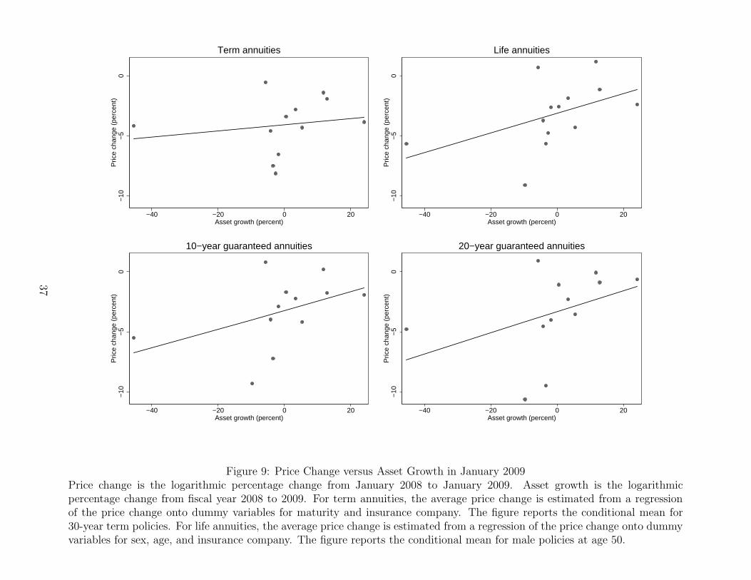
Figure 9 is a scatter plot of the percentage change in annuity prices between January

2008 and 2009 versus asset growth from end of fiscal year 2007 to 2008. The four panels

represent term annuities, life annuities, and 10- and 20-year guaranteed annuities. In each

panel, the 13 dots represent the insurance companies in our sample in January 2009. The

linear regression line shows that there is a strong positive relation between annuity price

changes and asset growth. That is, the price cuts were deeper for those insurance companies

19

that experienced more adverse balance sheet shocks just prior to January 2009.

Our joint interpretation of Figures 8 and 9 is that insurance companies were able to

maintain a low leverage ratio in 2008 and 2009 by taking advantage of statutory reserve

regulation that allowed them to record far less than a dollar of reserves per dollar of future

insurance liability. The incentive to discount prices was stronger for those insurance compa-

nies that experienced more adverse balance sheet shocks and, therefore, had a higher need

to recapitalize.

5.2 Empirical Specification

Let i index the type of policy, j index the insurance company, and t index time. Based on

equation (18), we model the markup as a nonlinear regression model:

log

(Pi,j,t

Vi,j,t

)= − log

(1− 1

εi,j,t

)+ log

(1 + λj,tVi,t/Vi,t

1 + λj,tLj,t/Aj,t

)+ ei,j,t, (25)

where ei,j,t is an error term with conditional mean zero. This empirical specification makes

it clear that the Lagrange multiplier is primarily identified by cross-sectional variation in the

ratio of reserve to actuarial value across different types of policies. As reported in Table 1,

the data for most types of annuities are not available prior to July 1998. We therefore

estimate our pricing model on the sample from July 1998 through July 2011.

We model the elasticity of demand as

εi,j,t = 1 + exp{−β ′Xi,j,t}, (26)

where Xi,j,t is a vector of policy and insurance company characteristics. In our baseline

specification, the policy characteristics are sex and age. The insurance company character-

istics are the A.M. Best rating, the leverage ratio, asset growth, and log assets. We also

include a full set of time dummies to control for any variation in the elasticity of demand

over the business cycle. We interact each of these variables, including the time dummies,

20

with dummy variables that allow their impact on the elasticity of demand to differ across

term annuities, life annuities, and life insurance.

In theory, the Lagrange multiplier depends only on insurance company characteristics

that appear in equation (23). However, most of these characteristics do not have obvious

counterparts in the data except for φ, which is equal to the leverage ratio when the constraint

binds (i.e., φ = L/A). Therefore, we model the Lagrange multiplier as

λj,t = exp{−γ′Zj,t}, (27)

where Zj,t is a vector of insurance company characteristics. In our baseline specification, the

insurance company characteristics are the leverage ratio and asset growth. Our use of asset

growth is motivated by the reduced-form evidence in Figure 8. We also include a full set of

time dummies and their interaction with insurance company characteristics to allow for the

fact that the leverage constraint may only bind at certain times.

5.3 Empirical Findings

Table 2 reports our estimates for the elasticity of demand in the nonlinear regression model

(25). Instead of reporting the raw coefficients (i.e., β), we report the average marginal effect

of the explanatory variables on the markup. The average markup on policies sold by A or

A− rated insurance companies is 3.13 percentage points higher than that for policies sold by

A++ or A+ rated companies. The leverage ratio and asset growth have a relatively small

economic impact on the markup through the elasticity of demand. Every one percentage

point increase in the leverage ratio is associated with a 6 basis point increase in the markup.

Every one percentage point increase in asset growth is associated with a 4 basis point increase

in the markup.

Figure 10 reports the time series for the shadow cost of the leverage constraint for the

average insurance company in our data. The leverage constraint does not bind for most

21

of the sample period. There is evidence that the leverage constraint was binding around

January 2001 with a point estimate of $0.79 per dollar of excess reserves. The leverage

constraint was clearly binding in January 2009 with a point estimate of $4.58 per dollar of

excess reserves. The 95 percent confidence interval ranges from $2.78 to $6.39 per dollar of

excess reserves.

In Table 3, we report the shadow cost of the leverage constraint for the cross section

of insurance companies in our data that sold annuities in January 2009. The table shows

that there is considerable heterogeneity in the shadow cost of the leverage constraint. The

shadow cost is positively related to the leverage ratio and negatively related to asset growth.

In January 2009, MetLife was the most constrained insurance company with a shadow cost

of $13.38 per dollar of excess reserves. Metlife had a relatively high leverage ratio of 0.97 at

the end of 2008 and suffered a balance sheet loss of 10 percent from the end of 2007 to 2008.

American General Life Insurance Company was the least constrained insurance company

with a shadow cost of $1.41 per dollar of excess reserves.

6. Conclusion

This paper shows that financial constraints and the regulation of statutory reserves have a

large and measurable impact on insurance prices. More broadly, this paper provides micro

evidence for a class of macro models based on financial frictions, which is a leading expla-

nation for the Great Recession (see Gertler and Kiyotaki, 2010; Brunnermeier, Eisenbach,

and Sannikov, 2012, for recent reviews of the literature). We feel that this literature would

benefit from further empirical investigation on the cost of these frictions (i.e., structural

estimates of the Lagrange multiplier) in other parts of the financial sector, such as banking

and health insurance.

We also feel that further work is necessary on the optimal regulation of statutory reserves.

The current regulation causes the statutory reserve requirement to vary arbitrarily, both

22

over time and across different types of policies. While this exogenous variation is useful for

identifying the shadow cost of the leverage constraint, it does not seem optimal from the

perspective of insurance regulation. In the context of our model (18), a simple reserve rule

that achieves price stability is to set the reserve value equal to the targeted leverage ratio

times the actuarial value (i.e., Vi = φVi). Under this reserve rule, the insurance price would

always be the Bertrand price (21), even when the leverage constraint binds. Although this

simple rule may not be the socially optimal policy in a fully specified model, it seems like a

good starting point for thinking about optimal regulation.

23

References

A.M. Best Company, Inc. 2011. “Best’s Credit Rating Methodology: Global Life and Non-

Life Insurance Edition.”

Berry-Stolzle, Thomas R., Gregory P. Nini, and Sabine Wende. 2011. “External Financing

in the Life Insurance Industry: Evidence from the Financial Crisis.” Working paper,

University of Georgia.

Brunnermeier, Markus K., Thomas Eisenbach, and Yuliy Sannikov. 2012. “Macroeconomics

with Financial Frictions: A Survey.” Working paper, Princeton University.

Brunnermeier, Markus K. and Lasse Heje Pedersen. 2009. “Market Liquidity and Funding

Liquidity.” Review of Financial Studies 22 (6):2201–2238.

Charupat, Narat, Mark Kamstra, and Moshe A. Milevsky. 2012. “The Annuity Duration

Puzzle.” Working paper, York University.

Gertler, Mark and Nobuhiro Kiyotaki. 2010. “Financial Intermediation and Credit Policy in

Business Cycle Analysis.” Working paper, New York University.

Gurkaynak, Refet S., Brian Sack, and Jonathan H. Wright. 2007. “The U.S. Treasury Yield

Curve: 1961 to the Present.” Journal of Monetary Economics 54 (8):2291–2304.

Hortacsu, Ali and Chad Syverson. 2004. “Product Differentiation, Search Costs, and Com-

petition in the Mutual Fund Industry: A Case Study of the S&P 500 Index Funds.”

Quarterly Journal of Economics 119 (2):403–456.

Kiyotaki, Nobuhiro and John Moore. 1997. “Credit Cycles.” Journal of Political Economy

105 (2):211–248.

Mitchell, Olivia S., James M. Poterba, Mark J. Warshawsky, and Jeffrey R. Brown. 1999.

“New Evidence on the Money’s Worth of Individual Annuities.” American Economic

Review 89 (5):1299–1318.

24

National Association of Insurance Commissioners. 2011. “Accounting Practices and Proce-

dures Manual.”

Rothschild, Michael and Joseph E. Stiglitz. 1976. “Equilibrium in Competitive Insurance

Markets: An Essay on the Economics of Imperfect Information.” Quarterly Journal of

Economics 90 (4):630–649.

Stern, Hersh. 2011. “Annuity Shopper.” Vol. 26, No. 2.

Warshawsky, Mark. 1988. “Private Annuity Markets in the United States: 1919–1984.”

Journal of Risk and Insurance 55 (3):518–528.

Yaari, Menahem E. 1965. “Uncertain Lifetime, Life Insurance, and the Theory of the Con-

sumer.” Review of Economic Studies 32 (2):137–150.

25

Table 1: Summary Statistics for Annuity and Life Insurance PricesMarkup is defined as the logarithmic percentage deviation of the quoted price from the actuarial value. The actuarial value iscalculated using the appropriate basic life table from the American Society of Actuaries and the zero-coupon Treasury yieldcurve. The sample is semiannual from January 1989 through July 2011.

Number of Markup

Sample Insurance StandardPolicy starts in Observations companies Mean Median deviation

Term annuities:5-year January 1993 732 83 6.7 6.5 8.410-year January 1989 988 98 6.9 7.0 5.915-year July 1998 418 62 4.3 4.8 5.620-year July 1998 414 62 3.8 4.4 6.625-year July 1998 339 53 3.4 3.7 7.530-year July 1998 325 50 2.9 2.8 8.8

Life annuities:Life only January 1989 11,879 106 9.8 9.8 8.210-year guaranteed July 1998 7,885 66 5.5 6.1 7.020-year guaranteed July 1998 7,518 66 4.2 4.8 7.5

Universal life insurance January 2005 3,989 52 -4.2 -5.5 17.9

26

Table 2: Structural Model of Insurance PricingThis table reports the average marginal effect of the explanatory variables on the markupthrough the elasticity of demand in percentage points. The model for the elasticity of demandalso includes time dummies and its interaction effects for life annuities and life insurance,which are omitted in this table for brevity. The omitted categories for the dummy variablesare term annuities, A++ or A+ rated, male, and age 50. The t-statistics, reported inparentheses, are based on robust standard errors clustered by insurance company, type ofpolicy, sex, and age. The sample is semiannual from July 1998 through July 2011.

Explanatory variable Average marginal effect

Rating: A to A− 3.13 (17.69)Rating: B++ to B− 9.16 (13.28)Leverage ratio 6.13 (23.55)Asset growth 3.91 (15.08)Log assets 2.31 (40.53)Interaction effects for life annuities:

Rating: A to A− -2.26 (-17.94)Rating: B++ to B− -8.77 (-11.02)Leverage ratio 16.88 (26.27)Asset growth -5.58 (-19.58)Log assets -1.89 (-44.69)Female 0.27 (10.18)Age 55 0.25 (1.74)Age 60 0.60 (3.90)Age 65 0.83 (11.94)Age 70 1.14 (10.25)Age 75 1.45 (2.99)Age 80 1.80 (10.60)Age 85 2.36 (10.41)Age 90 3.28 (6.58)

Interaction effects for life insurance:Rating: A to A− -23.21 (-5.12)Leverage ratio 21.78 (3.02)Asset growth -30.05 (-5.27)Log assets -13.21 (-7.36)Female 0.18 (1.03)Age 30 2.38 (0.21)Age 40 0.62 (0.03)Age 60 0.18 (0.00)Age 70 0.64 (0.31)Age 80 0.65 (0.27)Age 90 24.12 (4.74)

R2 (percent) 48.51Observations 29,570

27

Table 3: Shadow Cost of the Leverage Constraint in January 2009This table reports the shadow cost of the leverage constraint for the cross section of insurance companies in our data that soldannuities in January 2009, implied by our estimated strutural model of insurance pricing.

A.M. Best Leverage Asset Shadow cost ofInsurance company rating ratio growth excess reserves

MetLife Investors USA Insurance Company A+ 0.97 -0.10 13.38Allianz Life Insurance Company of North America A 0.97 -0.03 10.47Lincoln Benefit Life Company A+ 0.87 -0.45 8.76OM Financial Life Insurance Company A- 0.95 -0.04 8.31Aviva Life and Annuity Company A 0.95 0.12 4.44Presidential Life Insurance Company B+ 0.91 -0.06 4.33EquiTrust Life Insurance Company B+ 0.95 0.13 4.12Integrity Life Insurance Company A+ 0.92 0.03 3.85United of Omaha Life Insurance Company A+ 0.91 -0.03 3.65Genworth Life Insurance Company A 0.90 0.00 3.13North American Company for Life and Health Insurance A+ 0.94 0.24 2.44American National Insurance Company A 0.87 -0.02 1.84American General Life Insurance Company A 0.87 0.05 1.41

28

010

020

030

040

0B

illio

ns o

f dol

lars

1994 1999 2004 2009Year

AnnuitiesLife insurance

Figure 1: Annual Premiums for Individual Annuities and Life InsuranceThis figure reports the total annual premiums paid for individual annuities and life insurance,summed across all insurance companies in the Best’s Insurance Reports. The sample is fromfiscal year 1992 through 2010.

29

−30

−20

−10

010

20P

erce

nt

Jan 1989 Jan 1994 Jan 1999 Jan 2004 Jan 2009Date

Average markup95% confidence interval

5−year term annuities

−30

−20

−10

010

20P

erce

nt



−30

−20

−10

010

20P

erce

nt



−30

−20

−10

010

20P

erce

nt



Figure 2: Average Markup of Term AnnuitiesMarkup is defined as the logarithmic percentage deviation of the quoted price from the actuarial value. The actuarial value iscalculated using the appropriate basic life table from the American Society of Actuaries and the zero-coupon Treasury yieldcurve. Average markup is estimated from a regression of markups onto dummy variables for A.M. Best rating and time. Thefigure reports the conditional mean for policies sold by A++ and A+ rated companies. The confidence interval is based onrobust standard errors clustered by insurance company. The sample is semiannual from January 1989 through July 2011.

30

−30

−20

−10

010

20P

erce

nt



Life annuities: Age 50

−30

−20

−10

010

20P

erce

nt



−30

−20

−10

010

20P

erce

nt



−30

−20

−10

010

20P

erce

nt



Figure 3: Average Markup of Life AnnuitiesMarkup is defined as the logarithmic percentage deviation of the quoted price from the actuarial value. The actuarial value iscalculated using the appropriate basic life table from the American Society of Actuaries and the zero-coupon Treasury yieldcurve. Average markup is estimated from a regression of markups onto dummy variables for A.M. Best rating, sex, and time.The figure reports the conditional mean for male policies sold by A++ and A+ rated companies. The confidence interval isbased on robust standard errors clustered by insurance company, sex, and age. The sample is semiannual from January 1989through July 2011.

31

−60

−40

−20

020

Per

cent

Jan 2005 Jan 2007 Jan 2009 Jan 2011Date


Universal life insurance: Age 30

−60

−40

−20

020

Per

cent



−60

−40

−20

020

Per

cent



−60

−40

−20

020

Per

cent



Figure 4: Average Markup of Universal Life InsuranceMarkup is defined as the logarithmic percentage deviation of the quoted price from the actuarial value. The actuarial value iscalculated using the appropriate basic life table from the American Society of Actuaries and the zero-coupon Treasury yieldcurve. Average markup is estimated from a regression of markups onto dummy variables for A.M. Best rating, sex, and time.The figure reports the conditional mean for male policies sold by A++ and A+ rated companies. The confidence interval isbased on robust standard errors clustered by insurance company, sex, and age. The sample is semiannual from January 2004through July 2011.

32

24

68

10P

erce

nt


AnnuitiesLife insurance10−year Treasury

Figure 5: Discount Rates for Annuities and Life InsuranceThis figure reports the discount rates used for statutory reserve valuation of annuities and lifeinsurance (with term greater than 20 years), together with the 10-year zero-coupon Treasuryyield. The sample is monthly from January 1989 through July 2011.

33

.7.8

.91

1.1

1.2

Rat

io o

f res

erve

to a

ctua

rial v

alue


5 year10 year20 year30 year

Term annuities

.7.8

.91

1.1

1.2

Rat

io o

f res

erve

to a

ctua

rial v

alue


Male aged 50Male aged 60Male aged 70Male aged 80

Life annuities

.7.8

.91

1.1

1.2

Rat

io o

f res

erve

to a

ctua

rial v

alue



10−year guaranteed annuities

.7.8

.91

1.1

1.2

Rat

io o

f res

erve

to a

ctua

rial v

alue




Figure 6: Reserve to Actuarial Value for AnnuitiesThis figure reports the ratio of reserve value to actuarial value for various types of annuities. The reserve value is calculatedusing the appropriate loaded life table from the American Society of Actuaries and the discount rate specified by StandardValuation Law. The actuarial value is calculated using the appropriate basic life table from the American Society of Actuariesand the zero-coupon Treasury yield curve. The sample is monthly from January 1989 through July 2011.

34

.81

1.2

1.4

1.6

Rat

io o

f res

erve

to a

ctua

rial v

alue



Figure 7: Reserve to Actuarial Value for Universal Life InsuranceThis figure reports the ratio of reserve value to actuarial value for universal life insurance.The reserve value is calculated using the appropriate loaded life table from the AmericanSociety of Actuaries and the discount rate specified by Standard Valuation Law. The actu-arial value is calculated using the appropriate basic life table from the American Society ofActuaries and the zero-coupon Treasury yield curve. The sample is monthly from January2005 through July 2011.

35

.88

.9.9

2.9

4.9

6.9

8Le

vera

ge r

atio

−5

05

1015

Ass

et g

row

th (

perc

ent)

1989 1994 1999 2004 2009Year

Asset growth (percent)Leverage ratio

Figure 8: Asset Growth and the Leverage Ratio for Life InsurersThis figure reports the median of the growth rate of total admitted assets and the leverageratio for the cross section of insurance companies in our data. The leverage ratio is the ratioof total liabilities to total admitted assets. The sample is from fiscal year 1989 through 2010.

36

−10

−5

0P

rice

chan

ge (

perc

ent)

−40 −20 0 20Asset growth (percent)

Term annuities

−10

−5

0P

rice

chan

ge (

perc

ent)


Life annuities

−10

−5

0P

rice

chan

ge (

perc

ent)



−10

−5

0P

rice

chan

ge (

perc

ent)



Figure 9: Price Change versus Asset Growth in January 2009Price change is the logarithmic percentage change from January 2008 to January 2009. Asset growth is the logarithmicpercentage change from fiscal year 2008 to 2009. For term annuities, the average price change is estimated from a regressionof the price change onto dummy variables for maturity and insurance company. The figure reports the conditional mean for30-year term policies. For life annuities, the average price change is estimated from a regression of the price change onto dummyvariables for sex, age, and insurance company. The figure reports the conditional mean for male policies at age 50.

37

02

46

Dol

lars

(pe

r do

llar

of e

xces

s re

serv

es)


Shadow cost of excess reserves95% confidence interval

Figure 10: Shadow Cost of the Leverage ConstraintThis figure reports the shadow cost of the leverage constraint for the average insurancecompany, implied by our estimated strutural model of insurance pricing. The confidenceinterval is based on robust standard errors clustered by insurance company, type of policy,sex, and age. The sample is semiannual from July 1998 through July 2011.

38

insurance regulation and policy firesales

Documents