integral optimization and some supply...
TRANSCRIPT
INTEGRAL OPTIMIZATION AND SOME SUPPLY CHAIN DEVELOPMENTS
by
RAFAEL GUILLERMO GARCÍA CÁCERES
Advisors
FERNANDO PALACIOS GÓMEZ
JULIÁN ARTURO ARÁOZ DURAND
A dissertation submitted to the Engineering Faculty in partial fulfilment to the
requirements for the degree of
DOCTOR OF PHILOSOPHY IN ENGINERING
UNIVERSIDAD DE LOS ANDES
COLOMBIA
2007

DEDICATION
I would like to dedicate this thesis to my parents, my brothers and to my daughter Maria
Paula and my wife Mónica, without whose support I would not have been able to
complete this work.

ACKNOWLEDGEMENTS
This thesis would not have come into being without the support and help from several
persons and I would therefore like to thank all of them.
The autor is greatly indebted to Dr. Fernando Palacios, Dr. Julián Arturo Aráoz and Dr.
Sergio Torres by their invaluable guidance, support and encouragement through all the
phases of graduate study and thesis preparation. Financial assistance received from
COLCIENCIAS, from the Pontificia Universidad Javeriana, from the Universidad de los
Andes. Finally, I want to thank to Dra. Elena Fernández by its support during my stay in
the Universidad Politécnica de Cataluña.

VITA
1998 - Graduated from Universidad Pedagógica y Tecnológica de Colombia, B,A..
1998 - 1999 - Assistance Ship, Universidad de los Andes, Colombia
2000 - Graduated from Universidad de los Andes, Msc., Colombia
2003 - Management Adviser, Almaviva S.A., Colombia
2003 – Consultant, OMA S.A., Colombia
2001 – 2006, Assistant Profesor, Departamento de Procesos Productivos, Facultad de
Ingeniería, Pontificia Universidad Javeriana, Colombia.
2001 – current, Director of the research group Logístikos. Classified “A” by
COLCIENCIAS
2007 – current, Associate Profesor, Departamento de Procesos Productivos, Facultad de
Ingeniería, Pontificia Universidad Javeriana, Colombia.
Publications
García, R.G., Aráoz, J.A., Palacios, F. (2007). Integral Análisis Method –IAM-.
European Journal of Operacional Research. In press.
Torres, S., García, R.G., Quintero, J.J. (2007). Costos de transacción en los servicios de
consulta externa: el caso de los hospitales de tercer nivel en Bogotá, Colombia. (2006).
Cuadernos de Economía: Latinoamerican Journal of Economics. In press.
Olaya, E.S., García, R.G., Torres, N.S., Ferro, D.C., Torres, S. (2006). Caracterización
del proceso productivo, logístico y regulatorio de los medicamentos. Vitae. 13(2) 69- 82.
García, R.G., Olaya, E.S. (2006). Caracterización de las cadenas de valor y
abastecimiento del sector agroindustrial del café. Cuadernos de Administración. 19(31)
197-217.
García, R.G. Monroy I.M., Guio, O.F. (2005). Análisis del sector generador de energía
eléctrica en Colombia. Revista de la Escuela Colombiana de Ingeniería. 57(1), 35-46

Torres, S., García, R.G., Quintero, J.J. (2005). Formas de CONTRATACIÓN de los
servicios de urgencias: una APROXIMACIÓN desde la economía de los costos de
transacción. Revista de Economía Institucional. 7,12: 209-237.
García, R.G. Caro, MP., Díaz, H., Sánchez, L.L., Carrillo, M.P.(2004). Metodología de
marco de referencia para localización de instalaciones. Ingeniería y Universidad.
8(2),139 – 157.
García, R.G., Correal, M.E. (2003). Análisis de los Componentes del PIB Colombiano.
Revista Ingeniería y Desarrollo, Universidad del Norte. 13(Enero – Julio), 69-84.
García, R.G., López, M., Torres, J.F. (2003). Aproximación a un Modelo de
optimización del despacho de agua en una red de acueducto. Ingeniería. 8(1), 58-63.
Pérez, Y.O, García, R.G. (2002). Medición de la eficiencia relativa de agentes
generadores de energía eléctrica en Colombia. Energética, 28(Diciembre), 27- 46.
Carrillo, M.P., Fiorillo, G.R. García, R.G. (2002). Modelo Analítico de Administración
de cadenas de abastecimiento en PIMES. Revista Ingeniería y Universidad de la
Pontificia Universidad Javeriana. Volumen 6, Numero 2, Julio- Diciembre
Software
García, R.G., Nieto, F., García, O.L. (2006). CMTD - ACADEMIC
García, R.G., Torres, S., Ferro, D.C. (2006). PREFERENTIAL DECISION -
ACADEMIC
Presentations
Intercambio de servicios de cirugía programada en hospitales de Bogotá, un análisis
soportado en SMAA. XIII CLAIO, Montevideo (Uruguay). 2006.
Economic analysis of link between end product dealers and health service promoters of
pharmaceutical supply chain of Bogotá, Colombia. 1er CNC-LOGISTICA. Zaragoza
(Spain). 2007.
Operations Research in Agroindustrial Supply Chain in Colombia. EURO XXI in
Iceland: 21st European Conference on Operational Research, Reykjavik (Island). 2006.

Representación del concepto de administración: una exploración en profesionales
colombianos. Encuentro Internacional en Administración. Cali, Colombia. 2007
Optimizacion of the colombian pharmaceutical supply chain including transaction cost.
Euro XXI in Iceland: 21st European Conference on Operational Research, Reykjavik
(Island). 2006.
Planeación estratégica y táctica de una cadena de abastecimiento doméstica para la
erradicación de minas antipersonales mediante robots In: XIII CLAIO, Montevideo
(Uruguay). 2006.
Optimization model to planning of supply chain on a palm oil plantation. Sixteen
Annual Conference of POMS - OM Frontiers: Winds of Change. Chicago (USA). 2005
Modelación matemática de una cadena de abastecimiento en el sector agroindustrial
colombiano: Palma Africana. XI ELAVIO Latin American Summer Workshop on
Operations Research. Villa de Leyva (Colombia). 2005.
SMAA y Análisis Discriminante Múltiple: aplicaciones al análisis de los límites entre
EPS e IPS de III nivel en Bogotá. XV Simposio de Estadística. Universidad Nacional de
Colombia. Paipa, 2005.
Análisis del sector generador de energía eléctrica en Colombia (año 2001). XV Simposio
Nacional de Estadística. Universidad Nacional de Colombia. Bogotá, 2005.
Determinación de la carga física y el consumo de oxígeno en conductores de carga y
pasajeros en la ciudad de Bogotá. VIII Congreso La Investigación en la Pontificia
Universidad Javeriana. Bogotá (Colombia). 2005.
Intercambio de Servicio de Consulta Externa en Hospitales de Bogotá, Colombia.
Management, Knowledge and Flexibility. Iberoamerican Academy of Management 4th
International Conference. Lisboa (Portugal). 2005
Una aplicación DEA al análisis del sector generador de energía eléctrica en Colombia.
XI ELAVIO Latin American Summer Workshop on Operations Research. Villa de
Leyva (Colombia). 2005.
Formas de CONTRATACIÓN de los servicios de urgencias: una APROXIMACIÓN
desde la economía de los costos de transacción. III Congreso Colombiano y I Encuentro
Andino de investigación de operaciones. Cartagena (Colombia). 2004.

Localización óptima multipropósito de instalaciones bajo incertidumbre. III Congreso
Colombiano y I Encuentro Andino de investigación de operaciones. Cartagena
(Colombia). 2004.
Determination of the Manual Material Handling Capabilities for Workers in Colombia.
ISOES - Conference Proceedings entitled “Quality of Work and Products in Enterprises
of the Future”. Munich (Germany). 2003.
Statistical analysis of the nature of Colombian Gross National Product. Simposio en
Investigación Operativa. Buenos Aires (Argentina). 2003.
Measuring the relative efficiency of electric power generating agents in colombia using
data envelopment analyses analices. Joint International Meeting IST. Istanbul (Turkey).
2003.
Differences between Anthropometrics of Workers and College Students in selected
Measurements. XVII Annual Conference de la International Society for Ergonomics and
Safety (ISOES). Munich (Germany) 2003.
Measuring the relative efficiency of electric power generating agents in Colombia.
Simposio en Investigación Operativa SIO'2003. Buenos Aires.(Argentina).2003.
Approximation to a model of optimal water flow dispatch in an aqueduct network.
Simposio en Investigación Operativa SIO'2003. Buenos Aires (Argentina). 2003.
Análisis de los Componentes del PIB Colombiano. XII Congreso de Colombiano de
Estadística, Simposio Colombiano de Procesos Estocásticos. Universidad Nacional de
Colombia. Bogotá (Colombia).2002.
Análisis de los componentes del Pib Colombiano (versión 1). XII Congreso de
Estadística, Simposio Colombiano de Procesos Estocásticos. Bogotá (Colombia). 2002.
Hypothetic optimization model of supply chain on a palm oil plantation. International
conference on industrial logistics. Montevideo: International Centre for innovation and
Industrial Logistics (ICIIL), 2005. p.193 – 202.
Field of Study

Optimization, Statistics, Applied Mathematical, Logistics, Production, Decision Theory,
Supply Chain Management.
Awards and Honours
Premio Bienal al Investigador Javeriano, 2007
Doctoral Scholarship - Colciencias, 2003
Master Scholarship - Universidad de los Andes (Programa Universidad Empresa), 1998
Best Work of degree Adviser. Industrial Engineering, 2003 and 2005.
Degree of honor in Industrial Engineering - Universidad Pedagógica y Tecnológica de
Colombia (UPTC) – 1998.
Undergraduated Scholarship, UPTC. (1994,1995,1996,1997)

TABLE OF CONTENTS
LIST OF TABLES……………………………………………………. ……….. … . ..... i
LIST OF FIGURES…...…………………………………………………………………iii
OBJECTIVES OF THE RESEARCH………………………………………………… iv
ABSTRACT AND RESEARCH ORGANIZATION…………………………………..vi
INTRODUCTION.…………………………………………………………………….xvii
Practical Application……………….………………………….…………….xvii
Supply Chain Governance Forms…………….……………………………….xx
1. CHAPTER 1. Tactical and operative optimization of the supply chain in the oil palm
industry…………………………………………………………………………………...1
1.1 Introduction……………………………………………………………………2
1.2 Literature review….………………………………………………………….. 6
1.3 The Model……..….………………………………………………………….. 7
1.4 Solution Procedure…………………………………………………………...17
1.5. Conclusions…………………………………………………………………..18
1.6. Sensibility Analysis.………………………………………………………….28
1.7. References……………………………………………………………………29
CHAPTER 2. Planning of a Supply Chain for Anti-Personal Landmine disposal by
means of Robots.………………………………………………………………………..31
2.1 Introduction…………………………………………………………………..32
2.2 Background…………………………………………………………….…….35
2.3 The model……………………………………………………………………36
2.4 Solution Procedure 1…………………………………………………………49
2.5 Solution Procedure 2…………………………………………………………53
2.6. Sensibility Analysis.………………………………………………………….54
2.7. Conclusions…………………………………………………………………..58
2.8. References……………………………………………………………………58
2.9. Appendix A…………………………………………………………………..60

CHAPTER 3. Costos de Transacción y Formas de Gobernación de los Servicios de
Consulta en Colombia: un estudio empírico……. ………………………...................61
3.1 Introducción…………………………………………………………………..62
3.2 Elementos del contexto de los Servicios de Consulta Externa……………….64
3.2.1 Legislación sobre las formas de contratación y pago en el Régimen
Contributivo……………………………………………………………………………..64
3.2.2 La consulta externa en los hospitales de tercer nivel……………………66
3.3 Marco Teórico………………………………………………………………..67
3.4 Metodología de Investigación...……………………………………………...74
3.4.1 Instrumento y medición………………………………………………………….74
3.4.2 Análisis de Información…………………………………………………………78
3.5 Resultados…………………………………………………………………...78
3.5.1 Descripción de la Población…………………………………………………...78
3.5.2 Análisis de las características de la decisión con SMAA.…………………..79
3.5.3 Análisis del error de contratación: Pruebas estadísticas preliminares…..85
3.5.4 Análisis Discriminante Múltiple –ADM-.....................................................87
3.6 Descripción de Resultados.............................................................................91
3.7. Referencias………………………………………………………………….93
3.8. Anexo B..........................................................................................................97
4. CHAPTER 4. Integral Analysis Method – IAM……………………………………1014.1 Introduction……………………………………………………………….
10Error! Bookmark not defined.
4.2 Background………………………………………………………………..103
4.3 The IAM Process………………………………………………………….104
4.3.1 Definition of the Problem ……………………………………………..106
4.3.2 Cardinal Analysis.………………………………………………………106
4.3.3 Ordinal Analysis.………………………………………………………..108
4.3.4 Integration Analysis……………………………………………………………113
4.4 Practical application of IAM……………………………………………..117
4.4.1 Definition of the problem………………………………………………..117

4.4.2 Cardinal Analysis……………………………………………………….119
4.4.3 Ordinal analysis…………………………………………………………122
4.4.4 Integral analysis…………………………………………………………124
4.5 Conclusions……………………………………………………………......126
4.6 References…………………….…………………………………………..126
5. INTRODUCTION REFERENCES ……………………………………………….127

LIST OF TABLES
Table 1.1. Different possible scenarios of the harvesting stage……………………………...20
Table 1.2. Scenarios of the transportation stage between stockpiling centers……………… 22
Table1.3. Scenarios of the transportation stage between CAEs and the plant……………… 25
Table 1.4. Main features of the costs studied in the supply chain…………………………...26
Table 2.1. Average unitary cost percentage structure of the supply chain…………………...55
Table 3.1. Dimensiones de las Formas de Gobernación del Intercambio en el Sector Salud..68
Table 3.2. Síntesis Resultados Análisis de Confiabilidad……………………………………78
Table 3.3. Distribuciones de Probabilidad –Datos porcentuales-…………………………….80
Table 3.4. Utilidades típicas de cada variable para las formas de gobernación alternativas...82
Table 3.5. Rangos de los Vectores de los criterios que soportan a cada alternativa…………82
Table 3.6 . Índices de Aceptabilidad…………………………………………………………84
Table 3.7. Normalidad de los Factores……………………………………………………….86
Table 3.8. Prueba de Correlación entre los Factores………………………………………...86
Table 3.9. Prueba de Homogeneidad de Varianza de las categorías de los Factores………...87
Table 3.10. Prueba de Homogeneidad de las matrices de Covarianza……………………….87
Table 3.11. Pruebas de igualdad de las medias de los grupos……………………………….88
Table 3.12. Coeficientes estandarizados de las funciones discriminantes canónicas………..89
Table 3.13. Coeficientes de Correlación de los Factores con la Función discriminante……..89
Table 3.13. Prueba de Homogeneidad de Varianza de las categorías de los Factores……….89
Table 3.14. Prueba de Validación de la Función Discriminante…………………….……….90
Table 3.16. Tabla de Clasificación…………………………………………………………...91
Table 4.1: Parameters and other symbols of the facilities location problem………………..118
Table 4.2: Stochastic cost parameters………………………………………………………119
Table 4.3. joint cardinal distribution of probability………………………………………...121
Table 4.4. marginal cardinal distribution of probability……………………………………121
Table 4.5. Adjusted joint probability distribution…………………………………………..122
Table 4.6. Expected cardinal value and deviation cardinal values…………………………122

Table 4.7. Expected overall value of the objective and Overall deviation value of the
objective for the location problem……………………………………………………..122
Table 4.8. Likert Table……………………………………………………………………...123
Table 4.9. Ordinal values associated to each class and Ordinal acceptability indexes……..123
Table 4.10. Ordinal ranking central values………………………………………………...124
Table 4.11. Joint integral indexes…………………………………………………………124
Table 4.12. Cardinal and ordinal result variables…………………………………………...124
Table 4.13. Integral acceptability indexes in ordinal ranking………………………………125
Table 4.14. Favourable weight ranges in ordinal ranking 1………………………..............125

LIST OF FIGURES
Figure 1.1. Supply Chain Scheme……………………………………………………………….3
Figure 1.2. Minimum variable costs of transportation between stockpiling centers, according to
transport type……………………………………………………………………………..23
Figure 1.3. Minimum fixed costs of transportation between stockpiling centers, according to
transport type…………………………………………………………………………....23
Figure 1.4. Minimum costs of transportation between stockpiling centers, according to cost
type……………………………………………………………………………………...24
Figure 1.5. Minimum variable costs of transportation between CAEs and the plant, according to
transport type……………………………………………………………………………………26
Figure 1.6. Minimal fixed costs of transport between CAEs and the plant, according to
transport type……………………………………………………………………………26
Figure 1.7. Minimum transport costs between CAEs and the plant, according to cost type…27
Figure 2.1. Effect of demand on minimum cost…………………………………………………56
Figure 2.2. Effect of robot scanning speed on minimum cost……………………………………57
Figure 2.3. Effect of helicopter capacity on minimum cost……………………………………...57

RESEARCH OBJECTIVES
The current research objectives can be summarized as follows:
1. Development of adequate mathematical procedures capable of dealing with
particular supply chain optimization problems.
2. Development of a methodology that allows to integrate cardinal and ordinal
criteria in stochastic optimization contexts.
3. Application of the developed methodology to supply chain practical cases.

ABSTRACT AND RESEARCH ORGANIZATION
The present doctoral dissertation introduces a series of contributions to current
optimization and decision problems, each of them within a single chapter issuing an
article on the topic, and including its corresponding literature review, study cases, and
associated research perspectives. Chapter one presents a mathematical model and a
solution procedure for an african palm oil sector's supply chain, dealing with fruit
collection, raw material transport from collection zones to stock centres, and extraction
of red oil and other primary derivates. The dynamic model developed takes into account
particular plantation conditions and production features, of which access roads to
collection zones and specific harvesting conditions are respective examples in the
current case. The paper presents a solution procedure based on commercial software,
together with a complete sensibility analysis of the most outstanding functioning
conditions of the supply chain.
Chapter two presents a mathematical model, two solution procedures and a sensibility
analysis supporting the strategic and tactical decision making process of an anti-personal
mine robotic erradication system’s supply chain. Strategic decision making includes
production and distribution infrastructure definition, factory location, and supply and
distribution channel selection. The two decision types are integrated in a single MIP
model (which is an aproximation of a more complex stochastic MNLIP), solved by
procedures based on commercial optimization software.
Chapter 3 issues a study on transaction costs resulting from commercial relationships
between Health Insurance Companies1 and Health Service Providers2 in rendering the
external consultation services commanded by the Solidarity and Social Security Health
1 These companies are locally known as “Empresas Promotoras de Salud”, which means “Health Promoting Companies”, and gives raise to their abbreviation as EPSs. 2 These companies are locally known as “Instituciones Prestadoras de Servicios (IPSs)”, which means “Health Providing Institutions”.

General System (SSSHGS)3 in Bogotá, Colombia. In order to obtain the necessary
information for the analysis, a survey was conducted on levels 3 and 4 IPSs, which hold
the largest and more complex service offers. The information was analyzed by means of
Discriminant Multivariate Analysis (DMA) and a Deterministic version of Stochastic
Multicriteria Acceptability Analysis (SMAA). As a result, a complete analysis was
obtained, not only allowing to determine the most efficient governance forms at
reducing the transaction costs between the two mentioned agent types, but also the
reasons why they are established.
Finally, chapter 4 introduces the new Integral Analysis Method (IAM), presenting both
its theoretical background and its practical application to a location problem. This
methodology integrates cardinal and ordinal aspects of combinatorial stochastic
optimization problems in four stages: problem definition, cardinal analysis, ordinal
analysis and integration analysis. Integrating concepts from SMAA, Monte Carlo
Simulation, Optimization Techniques and Probability Elements, IAM was used to
determine an optimal location for a Colombian coffee marketing company.
3 "Sistema general de Solidaridad y Seguridad Social en Salud", stands for its spanish name.

INTRODUCTION AND CONCEPTUAL APPROACH
Advances in optimization have allowed the modelling of a great number of problems,
which have been “solved” with the aid of new computational advances that include
mathematical solution procedures capable of dealing with cardinal variables. The
solution procedures include algorithms to solve non – linear, integer, combinatorial,
stochastic, global, and multiobjective problems, which have succeeded in small and
medium optimization instances. Exceptions are the linear, quadratic, integer and
combinatorial problems with special structures, which can be solved efficiently in large
instances. On the other hand, techniques that allow approximate solutions are now
having relevant success for integer, combinatorial, multiobjective, non – linear and
global problems. Among these techniques there are heuristic, metaheuristic and hybrid
ones (those that combine algorithms and heuristics). But despite such advances, it has
not yet been possible to develop any technique that is capable of handling qualitative
aspects in optimization problems. In sum, it can be said that in many cases, the currently
existing procedures do not allow finding solutions that are more in accordance to reality,
due to epistemologic and technical limitations that make it difficult to treat both
quantitative and qualitative aspects at the same time in these decision contexts. In order
to work out such solutions, an Integral Analysis Method (IAM) is developed in chapter
4.
Practical Application: Supply chains
The outset of the supply chain concept and its practical applications appeared in the
80’s, not only as a response to the globalization process, which germinated by the time,
but also as a consequence of the apparent impossibility that single agents would find to
increase their competitiveness and participation in the market by themselves [Johnson et
al., 1999]. In this sense, various authors [Giannakis and Croom, 2004; Lummus and
Vokurka, 1999] have established that current competition does not actually take place
among firms, but among supply chains.

The need to increase collaborative efforts among different agents, experimented by the
industrial sector [Porter, 1987], along with an inefficient answer on the part of the
academic community, brought up an abundant conceptual proliferation and non-
standardized literature. Such proliferation prevented faster theoretical developments in
supply chain management theory, which was only later incipiently conceived by the
pioneer work of Paulraj [2002]. Such non-standardization has taken place at
fundamental conceptual levels, including for example, discrepancies in the very
definition of what a supply chain is, coming from a variety of literature sources ranging
from APICS dictionary, the Supply Chain Council, the Institute for Supply Chain
Management and the Global Supply Chain Forum, to those provided by different
practitioners and theorists on this issue.
As a result, the supply chain concept has been continuously changing since its inception,
from the initial thought just regarding material control [McKone-Sweet et al., 2005], to a
variety of proposals currently in use [Lambert et al., 2005]. These proposals conceive
the supply chain concept as a series of activities, from raw material to final consumer
stages, involving information and resource flows [Brennan, 1998, Lambert et al, 2005],
and entailing several necessary aspects, like demand management, suppliers, supply
orders, logistics, inventory, and manufacturing planning [Brennan 1998; Quinn, 1997;
Lummus and Vokurka 1999]. Besides these aspects, Lambert et al. [1988] have included
some additional items like customer relationship management, customer service,
manufacturing development and customization. To sum it up, supply chains can be said
to imply a multi-organizational effort to manufacture and place goods, from the
supplier’s supplier to the customer’s customer. That is, all activities involved in getting a
product to its final consumer, including raw material and part sources, manufacturing
and assembly, storage and stock monitoring, order reception and shipment management,
distribution, delivery, and necessary information systems to control it all [Tan, 2001].
Notwithstanding, as will be shown next, not all of these aspects have been dealt with in
the supply chain literature.

Supply chain optimization is a widely developed topic, as it results from the variety and
abundance of works in this field, some of which are referred in the literature reviews
here cited [Aikens, 1985; Cohen and Lee, 1988; Bhatnagar et al., 1993; Geoffrion and
Powers, 1995; Thomas and Griffin, 1996; Vidal and Goetschalckx, 1997; Tsay, 1999
and Goetschalckx et al., 2002], and have led to relevant considerations in supply chain
decision making, which have been recently included by Paulraj [2002] within the
development of a theoretical framework on the topic.
Two types of decision making can be found concerning supply chains: strategic and
tactical, respectively dealing with long and medium term actions [Shapiro, 2001;
Harrison, et al., 2003]. Strategic decisions are the most important ones, since they have a
stronger impact on supply chain financial operation and viability [Shapiro, 2001;
Harrison, et al., 2003]. Their optimization has allowed a 10% average cost reduction,
ranging from 5% to 60% in some cases; while service times have been reduced by 25%
to 75%, averaging 30%. Such improvements have allowed substantial increases in
manufacturing throughput, reliability, and customer satisfaction [Harrison, et al., 2003].
Strategic decisions in optimization contexts have to do with location and capacity of
manufacturing plants and distribution centers, procurement channels, suppliers, and
logistic considerations about distribution [Harrison, et al., 2003].
On the other hand, optimum tactical and operational decisions in the supply chain are
associated to a variety of items, like lead time fulfillment, bill of materials, logistic break
– up, issues concerning international supply chains, distribution and manufacturing
aspects such as scale economies, and the establishing of dynamic and static inventories
and appropriate raw material and product flows in multi – stage supply chains [Harrison,
et al., 2003]. As a pioneer practical application, chapter one presents the tactical
modelling of an African palm oil sector's supply chain, issuing some frequently omitted
aspects in the literature, like periodical programming of the collection and delivery fleet,
or production set-up.

In spite of the advances in strategic and tactical decision making optimization, only few
works have integrated both types of decision within a single model. Such is the scope of
the paper presented in chapter two, in dealing with an antipersonal mine erradication
system’s supply chain.
Supply Chain Governance Forms
A series of different standpoints, namely strategic fields [Williamson, 1991], marketing
[Dwyer et al., 1987], and supply chain management [Grover and Malhotra, 2003] have
clearly recognized how the competitive development of organizations is strongly
affected by the way they interact to exchange goods and services. In this sense, the
supply chain structure has a two-fold effect, comprising both cost reduction [Brennan,
1998; Mckone-Sweet et al., 2005] and generation of added value [Mckone-Sweet et al.,
2005].
Linked to the globalization process and to new developments in computer technology
and telecommunications, and with the consequent competitiveness intensification,
important changes have emerged for supply chains [Lambert et al., 2005]. One of the
most important has to do with the way in which economic agents should deal with one
another in order to minimize their costs. On the one hand, a vertical disintegration
process, encouraged by the need of reducing operational risks has been taking place
[Jones et al., 1997; Lummus and Vokurka, 1999], therefore concentrating organizational
efforts in the development of central competences [Prahalad and Hamel, 1990].
However, such disintegrated structure has been experimented, for example, in the
exchange with intermediate goods and logistic service suppliers with whom marketing
relationships are not clearly established, but (with whom) formalization becomes
imperative, consequently determining the cooperation relationship to be preferred as a
governance form [Heide, 1994], [Shin et al., 2000]. All these factors have rendered
complex exchange relationships [Dwyer et al., 1987], and a high interpenetration degree

among different agents in the chain [Heide, 1994], therefore allowing different
governance forms to coexist.
A governance form is defined as the institutional framework in which contracts support
the transaction of goods and services between agents [Palay, 1984]. The different
governance forms that can be found in supply chains are: vertical integration [Kim and
Frazier, 1996], several agreement types on bilateral cooperation [Arzt and Norman,
2002; Dwyer et al, 1987, Heide, 1994; O’Toole and Donaldson, 2000], supply networks
[Moriarty and Moran, 1990], and market forms [Artz and Norman, 2002].
Although decisions that are only based on operational costs are known not to allow an
overall estimation of supply chain costs (which should also include transaction costs
[Coase, 1937; and Williamson, 1975, 1985, 1991, 1993]), the optimization techniques
that support the supply chain decision making process have been mainly focused on
financial measurements of performance [Beamon, 1998], despite the strategic and
tactical importance of supply chain governance form optimization, which has only
recently been approached [Tsay, 1999] by works related to contractual aspects [Weng,
1995; Gu, 2001]. Governance forms appear then as a tacit deficiency of supply chain
optimization literature, and deserve to be considered as a fruitful and relevant research
perspective [Paulraj, 2002], [Grover and Malhotra, 2003]. For this reason, chapter three
presents a pilot test developed to identify the most efficient governance forms at
reducing transaction costs in a specific echelon of the pharmaceutical supply chain in
Bogotá.

CHAPTER ONE
Send to Applied Mathematical Modelling
Status: Second review

Tactical and operative optimization of the supply chain in the oil palm industry
Rafael Guillermo García Cáceres*
Mario Ernesto Martínez Avella**
Fernando Palacios Gómez ***
Abstract
This paper shows a dynamic mathematical model of the supply chain for the harvest and
oil extraction from oil palm. The mathematical programming model developed has
nonlinear and mixed integer features both in the objective function and the constraints,
implying a NP-hard problem. In the solution process, the nonlinear nature of the
problem is treated, redefining adequately some original variables and modifying certain
constraints; as result, an equivalent MIP model is obtained. The model was validated
using an experiment based in computational simulations.
Key words: Mathematical programming applications, integer programming, linear
programming, logistics.
1.1. Introduction
The plantation where the supply chain actually takes place is divided into sections which
are made up of land plots aligned by furrows sown at appropriate distances so as to leave
the necessary space for plants to grow and to facilitate fruit harvest. Harvest is organized
in groups of workers who load the wheelbarrows; these are pulled by animals force
through rough and difficult-to-transit paths. The various groups of workers are
responsible for harvesting fruit in a pre-established number of land plots; they must left
their daily load at internal stockpiling centers (hereinafter referred to as CAIs) located on
This article is the result of a research project “Optimization of Agro-industrial Chains in Colombia” carried out by the Universidad de la Sabana and the Pontificia Universidad Javeriana with the financial support of COLCIENCIAS (Spanish acronym for Colombian Institute for the Development of Science and Technology ‘Francisco José de Caldas’) and the Universidad de la Sabana.Email: *[email protected], **[email protected], ***[email protected].

the access roads. On the other hand, the harvest zone allotted to each group of workers
must be previously determined per each production cycle.
Figure 1.1. Supply Chain Scheme
The road network is divided into zones which are passed through by truck-type vehicles
in which the fruit are taken from CAIs to larger external stockpiling centers (hereinafter
referred to as CAEs), located on various road intersections. One important consideration
for the vehicles used is that these guarantee the load security under difficult
circumstances: road, weather and geographical conditions. On the other hand,
plantations are connected to main roads for bulk transportation purposes from CAEs to
processing plants, which represents a final transport echelon. Vehicles running through
this echelon must comply with certain technical requirements concerning capacity and
speed. The whole process is supported by equipment used for lifting the fruit from the
floor in stockpiling centers and loading it into vehicles; this task can be performed by
attaching certain devices to the vehicles or independently by cranes or forklift trucks.

The throughput capacity of the harvest plots (CAI’s) is concretely defined by a multiple
of the throughput capacity of the supplying trucks so that these vehicles exclusively
perform trips between the CAI’s and the CAE which is allotted to the harvest zone,
without having to approach other CAI’s in order to fill their maximum capacity. Thus,
by cutting down the trip length, the most efficient flow of prime material is achieved at
this echelon of the supply chain.
Unlike the fruit picking itself, which is carried out in a single-step activity, the transport
of the crop is divided into two stages: the first consists of the hauling between the CAI’s
and the CAE’s, the second between the CAE’s and the oil extraction plant. Both require
a separated organizational scheme. The performance at each echelon is determined by
the actual throughput capacity of the trucks, be they company owned or subcontracted.
The way of assigning the real hauling task for each kind of vehicle varies, because the
reliability on subcontracted trucks depends on their lower availability, since every
horizon planning anew the equal conditions for each cooperative have to be established
due to the fact, that the productivity of each lot differs yearly with the age of trees.
Consequently, the company-owned trucks are assigned to the areas with less prospected
productivity. As becomes obvious, the procurement of work force, animals, and required
vehicles has to be ascertained previously to each harvest season. This includes as well
the computation of trips necessary to be carried out in order to satisfy the balance
between the expected supply and demand. In the Figure 1.1 the graphical presentation of
the supply chain under scrutiny is showed.
As a preventive measure for assuring the continuity of the productive process, it must
begin only when the raw material in stock at the plant has reached a pre-established
minimum amount. This measure is useful to avoid losses caused by over-costs generated
by interruptions unforeseen in the productive system.
The production involved in the extraction process includes red oil obtained from the fruit
flesh, as well as palm oil and palm pulp obtained from the fruit bone by a pressing

process. Other products, such as fibber and husk, are obtained and used as fuel and
fertilizers. These products are then stored and finally sold or consumed in the productive
process.
During the process, raw material inventories are generated in the stockpiling centers, and
in the warehouses where raw material, and finished products are kept in stock, bounded
by their related throughput capacity. Inventories force administrators (particularly in the
case of raw materials) to adopt preventive measures to avoid perishing of crops. In order
to embody this consideration into the development of systematization whose product is
this article, the timing can be tightly linked to time span which the perishable product
allows, because due to the periodicity of the productive cycle of the oil palm and
because of the loss of oil quality caused by fruit over ripeness once the harvesting time
has passed, land plots in their productive time should be totally harvested at the end of
productive cycle.
Some aspects, such as provision capacity and uncertainty of demand are irrelevant in
this supply chain, because it is always possible to have well-adjusted production curves
based on the age of the land plot, and because demand is usually guaranteed by the
market that buys all available production, which late on is sold to refineries (an echelon
which is not being investigated in this article). However, more general considerations
can be taken into account in the latter case as new possible applications of the research.
In order to rationalize production, oil producing companies have opted for different
forms of work organization that foster the intervention of third parties (out sourcing) in
the process. A frequently used organizational form leaves harvest and transportation
tasks to cooperatives subcontracted. Another reason for low competitiveness is the
almost total lack of sophisticated technology for decisions making techniques that would
optimize raw material and product flow in the chain and minimize the costs involved in
harvest, transport and production. In summary, the logistic and production operations in
the palm oil industry are likely to be improved because of the system’s complexity and

the little support available for the decision-making processes that hamper planners’
tasks.
This research project emerged as one of the Government’s measures to improve oil palm
agricultural industry competitiveness. The work presented here includes a description of
the characteristics of the oil palm supply chain; based on the analysis of this chain, a
model for the harvest and oil extraction echelons of the supply chain is presented, which
can be reproduced due to the similar production characteristics shared by other
agricultural industries [FAO, 2004].
1.2. Literature review
One first review was developed by Aikens (1985). The author offers a description of the
relevant aspects on supply chain modelling of single echelon systems with deterministic
demand. The fundamental tactical aspects were associated with distribution of raw
materials and final products. The size of the problems was limited by the absence of a
computationally adequate MIP optimizer. On the one hand, as was indicated by Aikens,
dynamic modelling aspects and handling of inventories associated to an agent were
developed [Cohen and Lee, 1988]. A later development is focused towards a better
coordination of the logistics operations between the different stages within the supply
chain (procurement, production and distribution), a special attention has to be drawn to
the publications by Thomas and Griffin (1996). The considered aspects included:
capacities of the procurement and distribution channels, and bill of materials. With
regard to the solution heuristic procedures supported in commercial software were
developed [Goetschalckx et al., 2002], that resulted in satisfactory practical
performances, which is supported by [Vidal and Goetschalckx, 1997]. Finally, Eskigun
et al. (2005) take into account the constraints in transportation capacity imposed by a
limited number of vehicles in distribution centers, which are sent from production plants
to one single distribution center in a particular period of time. This work is an expansion
of the one carried out by Eskigun et al. (2001).

Some of the work done on the application of mathematical modeling in agro-industrial
supply chains includes that of López et al. (2001), who propose a solution to the problem
of high transportation costs for sugar cane grown in different remote fields and
transported to a central sugar-processing plant. Constraints include the need for steady
central supply, the means used in harvesting, the different types of transportation, and
the supply routes; sugar cane must be taken first to stockpile centers and transported to
the processing plant by train. Finally, Villegas, et al. [2006] introduce a model of the
coffee supply chain in Colombia whose objectives are to minimize costs and to
maximize service level, and involve distribution issues, similar to those being considered
in this article.
1.3. The model
In order to present the MINLP and MIP models, a consistent notation is presented as the
aspects of the supply chain are introduced.
Aspects taken into account
The aspects considered in the model are here treated in detail, as shown next:
Supply available in the planning horizon
Depending on the planning horizon, the harvest operation can be carried out totally or
partially. In the present case the situation is modelled by means of an inequality, which
can eventually be changed for an equality if the planning horizon coincides with the
critical harvesting period, in order to guarantee the quality of the product.
Indexes and Sets:
i : Land plots index, where i Є Ώ
t : Planning horizon index, where t Є T
Γ(i) : Internal stockpiling centers set supplied by land plot i

Parameters:
oit : Supply of raw material at land plot i in time period t. (input quantity / time period t).
Variables:
Xijt : Raw material transported between land plot i and storage deposit j in time period t.
(weight or volume quantity / time period t).
Constraint:
ΩioXTt
ti
Tt Γ(i)j
tij
(1.1)
Mass balance
The model is being conceived as a mass flow through a conservative multi-period
network which begins in the plantation and ends with the end product. Within the span
between harvesting plots and the production plant, stock surveillance of raw material
and products are being carried out, since the conditions of supply and demand influence
considerably the flow of raw material in the multi periodical net. The purpose of mass
balance constraints is to guarantee a conservative flow in the supply chain network.
Constraints modulate decisions concerning the size of inventories in stockpiling centers
and plant warehouses, as well as the flow through transport and harvest zones. The
accumulated stock of each product in a time period is equal to that product’s inventory
in the previous time period plus production minus demand during the period. On the
other hand the stock of raw material in a plant warehouse in a time period is equal to its
inventory in the previous time period, plus the raw material received, minus the raw
material used in production in the next time period. The equations representing these
relations are the following:
Indexes and Sets:
j : index of internal stockpiling centers, where j Є Γ
k : index of external stockpiling centers, where k Є Θ
p : index of products, where p Є P

Parameters:
dpt : Estimated demand of product p in time period t. (quantity of product p / time period
t).
rendp : Quantity of product p / Quantity of raw material. (percentage / product).
Variables:
I▫t : Raw material inventory at storage deposit ▫ in time period t, where ▫ Є (Γ U Θ).
(weight or volume unit / time period t).
JMt : Raw material inventory at storage deposit of plant in time period t. (weight or
volume unit / time period t).
JPpt : Product p inventory in plant warehouse in time period t. (product p units / time
period t)
MPt : Raw material used as production input in time period t. (weight or volume quantity
/ time period t).
Xjkt : Raw material transported between storage deposit j and k in time period t. (weight
or volume quantity / time period t).
Ykt : Raw material transported between CAE k and plant in time period t. (weight or
volume quantity / time period t).
Zpt : Product p produced in time period t. (quantity of product p / time period t).
Constraints:
Mass balance of raw material inventory at plant in the time period:
TtMPYJMJM tt
kk
tt 11 (1.2)
Mass balance of raw material inventory at internal stockpiling center:
TtΓ,jXXIIΘ(j) k
tjk
Ω(j) i
tij
tj
tj
1 (1.3)
Mass balance of raw material inventory at external stockpiling center:

TtΘ,kYXII tk
Γ(k)j
tjk
tk
tk
1 (1.4)
Mass balance of a product inventory in the planning horizon:
TP,tpdZJPJP tp
tp
tp
tp 1 (1.5)
Production
Indexes and parameters:
qp : Quantity of product p / Quantity of raw material. (percentage).
Constraint:
TtP,pMPqZ tp
tp (1.6)
Capacity
As can be seen further below, the flows and stocks are determined by the parameters of
performance and the throughput capacity of each stock. The constraints which occur in
this process are the following:
Indexes and parameters:
cp : Capacity to produce product p. (weight or volume units of product p / time period).
f▫ : Capacity to store raw material at storage deposit type ▫, where ▫ Є (Γ U Θ). (weight
or volume units / storage deposit).
u : Raw material stock capacity of plant warehouse. (weight or volume units).
Constraint:
Plant production capacity:
TtP,pcZ ptp (1.7)

Raw material stock capacity of plant warehouse:
TtuJM t (1.8)
Raw material inventory capacity at stockpiling centers:
Tt,ΘΓfI Ut (1.9)
Distribution capacity
The quantity of raw material transported per echelon in each time period is determined
by the loading capacity of each type of vehicle used, and the number of trips made by
them in the planning horizon; where both vehicles and number of trips are bounded. The
bounds of trip numbers by the vehicles in each echelon of harvesting and transportation
represent average values obtained by experience and which depend on the age of the
plantation the type of vehicle used, load safety and soil conditions in the zone. It must be
highlighted, that the entire character of the issue depends on the parameter of throughput
(load/speed) capacity of the trucks. The pertinent equations to represent this are the
following:
Indexes and Sets:
A : Edges set of the supply chain network. The set A is composed by the three types of
edges associated to the following pairwise sets : (Ώ, Γ)U(Γ, Θ)U(Θ, plant).
v : Vehicle property index, where v Є Ξ.
Parameters:
b▫▪v : Load capacity of type of transport v used between storage deposit ▫ and ▪, where
(▫,▪) Є ((Ώ, Γ)U(Γ, Θ)). (weight or volume units / type of vehicle).
bkv : Load capacity of type of transport v used between storage deposit k and plant.
(weight or volume units / type of vehicle).
h▫▪v : Maximum number of possible trips that a type of transport v can make between
storage deposit ▫ and ▪ in one time period, where (▫,▪) Є ( (Ώ, Γ)U(Γ, Θ)). (trips / time
period).

hkv : Maximum number of possible trips that a type of transport v can make between
CAE k and plant. (trips / time period).
Variables:
L▫▪vt : Number of vehicles type v used for transportation between storage deposit ▫ and ▪
in the time period t, where (▫,▪) Є ((Ώ, Γ)U(Γ, Θ)). (vehicles / time period).
Lkvt : Number of vehicles type v used for transportation between storage deposit k and
plant in the time period t. (vehicles / time period).
N▫▪vt : Number of trips made by transportation vehicle type v between storage deposit ▫
and ▪ in the time period t , where (▫,▪) Є ( (Ώ, Γ)U(Γ, Θ)). (trips / time period).
Nkvt : Number of trips made by transportation vehicle type v between CAE k and plant in
the time period t. (trips / time period ).
Constraints:
Maximum number of trips by echelon:
TtΞ,vA,)(hN ,vvt (1.10)
Quantity of raw material harvested and transported between stockpiling centers:
TtA,)(LNbX ,
Ξv
vtvtvt
(1.11)
Maximum number of trips between external stockpiling centers and plant:
TtvkhN vk
vtk ,, (1.12)
Quantity of raw material transported between external stockpiling centers and plant:
TtΘ,kMNbYΞv
vtk
vtk
vk
tk
(1.13)
Infrastructure Distribution

The corresponding bound for the vehicle fleet assigned to any given harvesting zone and
transportation are, in the case of outsourcing, previously defined through the conditions
of the contract agreed on with the cooperatives. As for the company-owned vehicles, this
depends on the availability of trucks in the respective harvesting zone, which are
determined by the by the transport operation projections and the geographical distances
where they are located in the moment of planning:
Indexes and Sets:
r : Harvest Zone index, where r Є R
s : Index of transportation Zone between Stockpiling Centers, where s Є S
Parameters:
m▫v : Maximum number available of vehicles type v at the zone type ▫ in one given time
period, where ▫ Є (R, S, Θ) (units / time period)
Variables:
M▫vt: Number of vehicles type v used at transportation zone type ▫ in time period t, where
▫ Є (R, S, Θ). (units / time period)
Constraints:
Number of work teams per harvest zone:
TtvR,rLMr(i,j)
vtij
vtr
(1.14)
Maximum number of harvest work teams:
TtvRrmM vr
Rr
vtr
,, (1.15)
Number of vehicles type v per zone of transportation between stockpiling centers:
TtΞ,vS,sLMsj,k)
vtjk
vts
(1.16)

Maximum number of vehicles type v for transportation zone:
Tt,vSsmM vs
Ss
vts
, (1.17)
Maximum number of vehicles type v used between external stockpiling centers and
plant:
Tt,vKkmL vk
Kk
vtk
, (1.18)
Demand
Production in a particular time period plus the input in the previous one must satisfy al
least the demand in that period.
Constraint:
TtPptpdt
pZtpJP ,1 (1.19)
Set up of production
For the production process to start there must be a minimum stock of inventory that
guarantees the continuity of plant production. In this way, interruptions in the production
process are avoided as well as their negative economic effects caused by the lack of
available raw material. This situation is modeled with the aid of binary variables that are
only activated (status = 1) if the minimum levels of inventory in the time period are
satisfied.
Parameters:
BIG : Positive number large enough to model production set-up
Π : Minimum raw material inventory at storage deposit of plant required to start
production (weight or volume units)
ε : Positive number small enough to model production set-up
Variables:
Otherwise0
periodtheinlevelstockminimuntheexceedmaterialrawofleveltheIf1 ttw
Constraint:
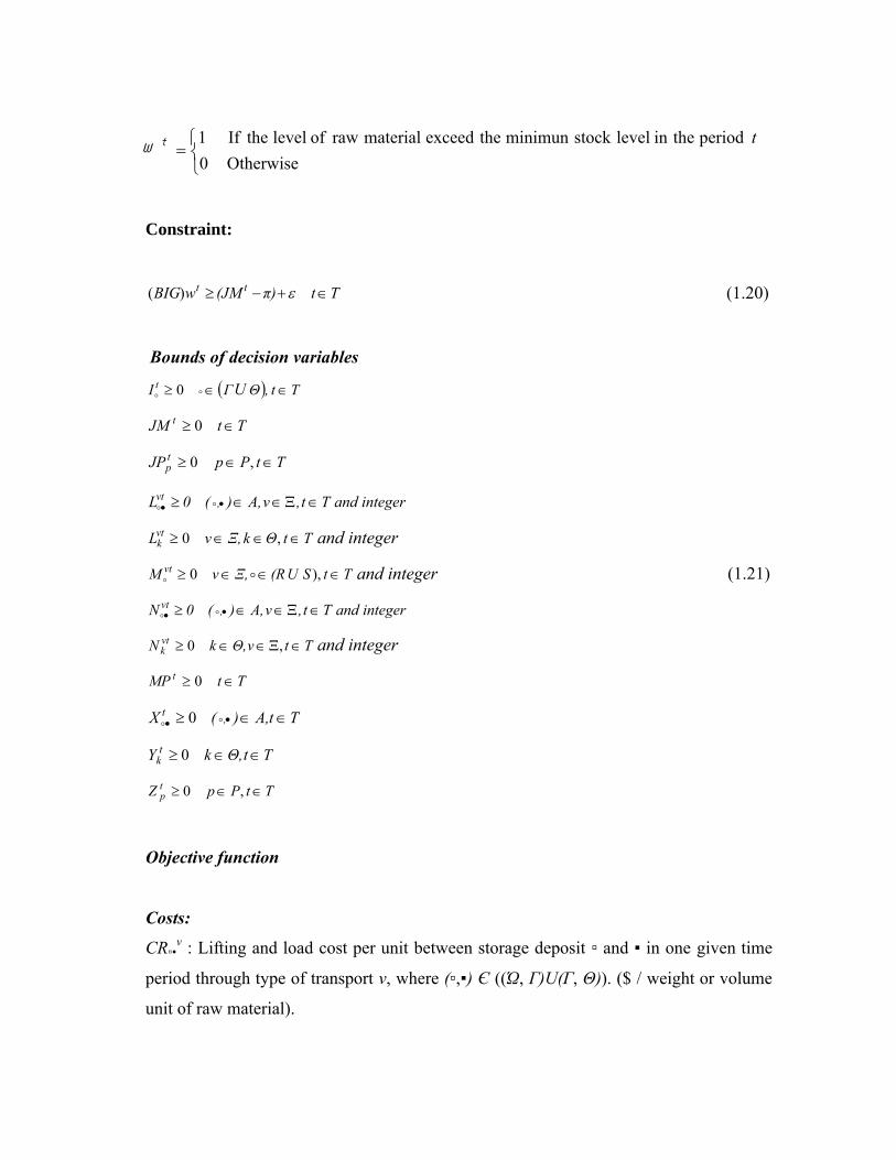
Ttπ)(JMwBIG tt )( (1.20)
Bounds of decision variables
Tt,ΘΓI Ut 0
TtJM t 0
TtPpJP tp ,0
integerandTt,vA,)(0L ,vt
TtΘkΞ,vLvtk ,0 and integer
TtSU(RΞ,vM vt ),0 and integer (1.21)
integerandTt,vA,)(0N ,vt
TtvΘ,kN vtk ,0 and integer
TtMP t 0
TtA,)(X ,t 0
TtΘ,kY tk 0
TtPpZ tp ,0
Objective function
Costs:
CR▫▪v : Lifting and load cost per unit between storage deposit ▫ and ▪ in one given time
period through type of transport v, where (▫,▪) Є ((Ώ, Γ)U(Γ, Θ)). ($ / weight or volume
unit of raw material).

CPp : Production cost per unit of product p. ($ / unit of product p).
CC▫▪v : Transportation cost per trip between storage deposit ▫ and ▪ in one given time
period through type of transport v, where (▫,▪) Є ((Ώ, Γ)U(Γ, Θ)). ($ / weight or volume
unit of raw material).
CCkv : Transportation cost per trip between storage deposit CAE k and plant in one given
time period through type of transport v. ($ / weight or volume unit of input).
CI▫ : Inventory cost per unit of raw material at storage deposit ▫ per time period, where ▫
Є (Ώ, Γ, Θ). ($ / unit of raw material).
CIPp : Inventory cost per unit of finished product p in plant warehouse. ($ / unit of
product p).
CF▫v : Fixed cost of type of transport v at zone ▫ in one time period, where ▫ Є (R, S, Θ).
($ / team in planning horizon).
CS : Set-up cost of production
t t t
t
t Θk Ξv
vtkk
Ξv
vt
p
tpp
t ΘΓ
t
t
t
t Ai,j t Θk Ξv
tk
tk
vk
vk
t Aj,k Ξv
vtjk
vtjk
vj
vjk
Ξv
vtijij
t p
tpp
)U()U( SR
(CS)wLCFMCFJPCIP(CI)I(CI)JM
LNbCCLNbCCXCRZCPMIN:
(1.22)
The objective here is to minimize the operation costs of harvesting and extracting oil
palm and products, taking into account the conditions already mentioned. The costs
presented in equation (1.22) represent respectively: production (C1), load and lifting raw
material inside land plots and CAIs (C2), load and lifting and transporting raw material
between stockpiling centers (C3), load and lifting and transporting raw material between
CAEs and plant (C4), raw material inventory in plant (C5), raw material inventory at
stockpiling centers (C6), product inventory in plant (C7), fixed cost at harvest and
internal loading zone (C8A, C8B), fixed cost at external loading zone (C9), production
set-up (C10).

1.4. Solution Procedure
The model here proposed is a nonlinear, mixed integer mathematical programming
equivalent to a MIP problem using necessary modifications. The process begins with the
transformation of variables in order to eliminate non-linearity:
Transformation of variables
What follows is a description of the transformations made to overcome the nonlinear
nature of the problem.
TtΞ,vA,LNα ,vtvtvt )( (1.23)
Ttv,kLN vtk
vtk
vtk , (1.24)
The equation (1.23) represents the number of trips made between the plots and the CAIs,
and the number of transportation trips made between CAIs and CAEs. On the other hand
the equation (1.24) describes the number of transportation trips completed between
CAEs and the plant.
Substitution of variables and rounding up and modification of constraints
The two new variables are substituted in the objective function. Furthermore, the
variable, defined by equation (1.23) is replaced in equation (1.11), and likewise, the
variable resulting in equation (1.24) is transferred to equation (1.13). On the other side,
these two new variables are redefined and rounded up using the procedure proposed by
Chvátal (1973) – Gomory (1958) which leads to modifying equations (1.10) and (1.12):
Number of trips for harvesting and between stockpiling centers – equation 1.10 -:
The number of trips made by harvesting teams in a particular time period between each
plot-CAI echelon cannot exceed the maximum number established.
TtΞ,vA,Lhα ,vtvvt )( (1.25)

where represents the highest full figure less or equal to the parameter. In order to
continue the procedure followed so far, equation (1.25) is modified. The procedure
replaces the inequality with an equality, including an additional integer variable and
define the bounds of it, as shown next:
TtΞ,vALhα ,vtvtvvt ,)(
(1.26)
Number of trips necessary for transportation between CAEs and plant -equation 1.12-:
Following the same procedure we obtain the expressions, as shown below:
TtΞ,vΘ,kδLhβ vtk
vtk
vk
vtk (1.27)
Bounds of decision variables:
TtΞ,vAα ,vt ,)(0 and integer
TtΞ,vA,,vt )(0 and integer
Ttv,k0β vtk , and integer (1.28)
Ttv,k ,0vtk and integer
The resulting model is made up of equations (1.1) a (1.9), (1.14) a (1.22), equations
(1.11) and (1.13) as modified by the solution procedure, equations (1.26) and (1.27)
suggested by the same procedure; and the bounds and their integer or linear condition
associated to the decision variables.
1.5. Sensibility analysis
The supply chain network (which is similar to the one shown in Figure 1.1) is
constituted by: eight harvest zones, each of them made up of three to five plots and one
CAI; five loading zones, each of which allows one to five CAIs and one CAE; and
finally one production plant. In the harvest zones the number of trips per day ranges

from four to nine; between stockpiling centers from four to eight, and between CAEs
and the plant, from three to eight. The seven periods studied correspond to a week.
Given that the studied network constitutes a considerable part of the entire network of
the company, the obtained results can significantly aid in the decision making process of
the whole supply chain.
The parameters under study were: loading capacity of a typical work team in the harvest
zones; loading capacity of the company owned vehicles used between stockpiling
centers; and of those used between CAEs and the plant; and finally, production capacity
and raw material set up inventory stock size. The conducted analyses show the changes
in the parameters in the directly related costs.
The process of the sensibility analysis implied changing one or two parameters at most,
which are indicated in each case. The offer equation was fixed as an equality (equation
1) and the inventories of the initial and final periods were fixed in 0. The majority of the
constraints contemplated in the model were included, except for those that correspond to
the bounds of the number of vehicles in the harvest and transportation zones (equations
1.15, 1.17 and 1.18). Such procedure takes as an intention to eventually adopt a single
operation system that is capable of rendering a more efficient functioning. The situation
does not suggest unfeasibility because, given the fact that we are dealing with just a
fraction of the network, the solutions can be considered to be optimal, since it is always
possible to satisfy the corresponding number of vehicles.
The different scenarios of the model were executed with the aid of a LINGO 10
commercial software package in a 256 MB RAM portable PC with Pentium 3
CELERON CPU and Windows XP operating system. The integer and linear
optimization gaps were respectively 8*10-5 and 5*10-7. The model comprises 1540
constraints and 10303 variables of which 7903 are integer, and seven are binary; the rest
of them being linear.

Analysis of harvesting capacity:
The sensibility analysis of the harvesting capacity studies the behaviour of the fixed and
variable costs of a significant part of the supply chain, along a series of different
scenarios previously defined by the decision makers, who considered the possible
changes in the parameters: maximum number of trips in each harvest zone; loading
capacity of the harvesting work team; type of animal used for the harvest (in the present
case two types of draught animals were studied, namely mule (type 1) and buffalo (type
2)); and finally, the associate unitary fixed cost of the combinations of these four
parameters, which takes into account different mechanical versions of the animal drawn
wheelbarrow and its maintenance. The treatment of the parameter "animal type" was
mutually exclusive, that is to say, the decision makers wanted the two possibilities to be
studied independently, and that no combinations were accepted between them.
The treatment of the parameters used in this analysis expresses the conditions and the
changes simulated by the model upon the current situation of the system, which is given
by the second scenario (number 2) in Table 1.1. Among such conditions we have ordinal
ones (animal type) and absolute cardinal ones (load capacity (bij), that appears explicitly
in tons). Similarly, the simulated changes include relative absolute ones (in the
maximum number of trips carried out between the plots and CAI associated to each
harvest zone (hij)) as well as percentage changes (in the case of the fixed unitary cost
(CFi)).
Table 1.1: Different possible scenarios of the harvesting stage
Scenario Type hij bij %CFi %C8A CPU Time
1 1 0 0.3 -14.29 22.6 120
2 1 0 0.4 0 0 95
3 1 0 0.5 14.29 -3.98 101
4 1 1 0.3 28.57 172.83 112
5 1 1 0.4 42.86 29.52 100
6 1 2 0.3 100 108.48 53
7 1 2 0.4 142.86 91.71 80

8 2 0 0.7 14.29 -28.09 98
9 2 0 0.8 42.86 -22.96 40
10 2 0 0.9 71.43 -17.52 77
11 2 0 1 100 -17.93 24
12 2 1 0.7 114.29 27.29 66
13 2 1 0.8 142.86 13.89 22
14 2 1 0.9 171.43 30.54 90
15 2 2 0.7 214.29 84.41 87
16 2 2 0.8 242.86 42.03 34
No changes were attributed by the model to the harvesting variable total cost (C2),
because the variable unitary cost (CRij) is established every year in agreement with the
syndicate, in terms of the gathered ton. In consequence, its value remains constant in any
possible scenario under analysis. That is the reason why the total harvesting cost is not
shown in Table 1.1. In this case, the variable that actually supports the decision making
process is the value of the total fixed cost (C8A). As it can be established from the
analysis, the best scenarios are related to the buffalo drawn wheelbarrow proposal,
especially when no harvesting work team current speed increasing changes are
undergone by the wheelbarrow. This condition contrasts with the current one, that
establishes the use of mules.
Analysis of transporting capacity between stockpiling centers:
This particular analysis studies the percentage changes in the variable and fixed costs
resulting from the operation of the vehicles between stockpiling centers in the
transportation zones, as far as they are induced by percentage changes in the througput
capacity of the typical company owned truck (bjk). The specifically studied costs are not
only the total ones (C3 and C8B) but their components too, here discriminated as those
resulting from the operation of the company owned truck fleet (C3P and C8BP) and of
the subcontracted one (C3T and C8BT). The variable costs mainly result from raw
material gathering and fuel supply for the vehicles; whereas the fixed costs result from

vehicle maintenance and insurances. The current condition can be observed in scenario 6
of Table 1.2, together with the rest of the studied scenarios.
Table 1.2: Scenarios of the transportation stage between stockpiling centers
Scenario bjk %C3P %C8BP %C3T %C8BT %C3 %C8B CPU Time
1 0.5 0 0.3 0 0 0 0 44
2 0.6 0 0.4 0 0 0 0 30
3 0.7 0 0.5 0 0 0 0 14
4 0.8 0 0.3 0 0 0 0 14
5 0.9 0 0.4 0 0 0 0 48
6 1 40 0.3 -5.13 -5.56 7.69 0 14
7 1.1 340.19 0.4 -46.69 -58.89 62.34 -5.56 208
8 1.2 428 0.7 -67.95 -90.24 69.23 -16.62 80
9 1.3 441.57 0.8 -73 -92.61 68.53 -16.7 117
10 1.4 451.57 0.9 -81.56 -96.61 63.17 -17.25 110
11 1.5 520 1 -100 -100 66.67 -19.44 184
12 2 600 0.7 -100 -100 92.31 -22.22 76
In order to obtain a clearer analysis of the behaviour of the costs in face of changes in
transporting capacity, the following three figures are used. As for the variable costs,
Table 1.2 shows how the total variable costs increase together with the capacity of the
company owned vehicle. Their biggest percentage change can be observed when the
capacity of the vehicle increases by 10 % above the current condition. This situation
tends to appear when the modelled operation mode determines the company's truck fleet
to dominate over the subcontracted one, as it can be clearly seen in Figure 1.2. The same
figure allows to see how if the capacity of the company owned vehicle falls ten percent
(or more) below the current condition, then the distribution can only be carried out on a
single mode of operation, which is in this case the subcontracted vehicle one. The
opposite situation turns out when the capacity of the vehicle increases by more than 50
% over the current condition.

0
20
40
60
80
100
120
0.5 0.6 0.7 0.8 0.9 1 1.1 1.2 1.3 1.4 1.5 2
Change in the company's own transportation capacity
Per
cent
age
chan
ge in
the
cost
s
%C3P
%C3T
Figure 1.2. Minimum variable costs of transportation between stockpiling centers, according to
transport type
0
20
40
60
80
100
120
0.5 0.6 0.7 0.8 0.9 1 1.1 1.2 1.3 1.4 1.5 2
Change in the company's own transportation capacity
Per
cent
age
chan
ge in
the
cost
s
%C8BP
%C8BT
Figure 1.3. Minimum fixed costs of transportation between stockpiling centers, according to
transport type
The analysis of the fixed costs is supported on Table 1.2 and Figure 1.3. The behavior of
the fixed total costs is in opposition to that of the variable total costs, as far as the former

decrease when the capacity of the company owned vehicles increases, although such
percentage changes are not as big as those of the variable costs. However, the more
remarkable variations in the fixed costs take place under similar conditions to those of
the variable ones. In sum, it can be said that fixed and variable costs present a similar
behavior at this distribution stage.
The following analysis compares the percentage of participation of the fixed and
variable costs in the transportation final costs of this stage. Figure 1.4 shows how the
fixed costs respond for more than 90 % of the costs of the transportation stage. This
explains why the variable costs increase together with the capacity of the company
owned vehicles, which is due to the fact that the decrease in the fixed costs
counterbalances the increase in the variable costs, therefore determining an overall
decrease of the total costs at this transportation stage.
0
20
40
60
80
100
120
0.5 0.6 0.7 0.8 0.9 1 1.1 1.2 1.3 1.4 1.5 2
Change in the company's own transportation capacity
Per
cent
age
chan
ge in
the
cost
s
%C3
%C8B
Figure 1.4. Minimum costs of transportation between stockpiling centers, according to cost type
Analysis of transporting capacity between CAEs and the plant:
This specific analysis studies the percentage changes in the costs of transport operations
between CAEs and the factory, as a consequence of percentage changes in the througput

capacity of the company owned trucks (bk). The studied costs include both the variable
and fixed total costs (C4 and C9) and their discriminated components C4P and C9P for
the proper operation, and C4T and C9T for the subcontracted operation. Given that the
company owned vehicles are provided with load lifting devices, the variable costs at this
transportation stage correspond to those of refueling, whereas the fixed costs mainly
result from vehicle maintenance and insurances. The different studied scenarios are
shown in Table 1.3, where the current operation corresponds to number 6.
Table 1.3: Scenarios of the transportation stage between CAEs and the plant
Scenario bk %C4P %C9P %C4T %C9T %C4 %C9 CPU Time
1 0 0 0 0 0 0 0 95
2 0.2 90 42.86 -4.48 -60 24.74 -5.66 128
3 0.4 190 60.71 -42.54 -84 29.38 -7.55 78
4 0.6 22.5 73.21 -100 -100 -62.11 -8.49 240
5 0.8 10 71.43 -100 -100 -65.98 -9.43 61
6 1 0 0 -100 -100 -69.07 -47.17 65
7 1.2 -7.5 0 -100 -100 -71.39 -47.17 191
8 1.4 -17.5 -14.29 -100 -100 -74.48 -54.72 98
9 1.6 -25 -21.43 -100 -100 -76.8 -58.49 130
10 1.8 -25 -25 -100 -100 -76.8 -60.38 190
11 2 -30 -26.79 -100 -100 -78.35 -61.32 93
12 3 -50 -28.57 -100 -100 -84.54 -62.26 120
The analysis of the transportation costs at this stage is supported on the same three types
of diagrams used in the previous stage. As it can be seen in the table above, the variable
total costs reach a maximum when the capacity of the company owned vehicles is 60 %
of the current one. The biggest percentage decrease occurs when the capacity of the
vehicle is 40% lower than the current condition, which happens when the transport is
totally done by the proper fleet (see Figure 1.5). The figure also allows to see that for the
transport to be carried out with a major participation of the subcontracted fleet, the
current capacity of the vehicle has to be reduced in more than 80 %.

0
20
40
60
80
100
120
0 0.2 0.4 0.6 0.8 1 1.2 1.4 1.6 1.8 2 3
Change in the company's own transportation capacity
Per
cent
age
chan
ge in
the
cost
s
%C4P
%C4T
Figure 1.5. Minimum variable costs of transportation between CAEs and the plant, according to
transport type
0
20
40
60
80
100
120
0 0.2 0.4 0.6 0.8 1 1.2 1.4 1.6 1.8 2 3
Change in the company's own transportation capacity
Per
cent
age
chan
ge in
the
cost
s
%C9P
%C9T
Figure 1.6. Minimal fixed costs of transport between CAEs and the plant, according to transport
type
The analysis of the fixed costs is supported on Table 1.3 and Figure 1.6. The fixed total
costs decline as the capacity of the company owned vehicles raises. Nevertheless, the

percentage changes are not as big as those of the variable costs. Without restricting the
number of vehicles of either transport fleet, the current operation should be carried out
by the company's one. The model predicts indeed, that such operating conditions allow
to reach capacities that are 40% above the current functioning. For capacity decrease
values that are close to 100% below those of the scenario of reference, the two
components of the fixed total costs of the transport operation at this stage show similar
participation percentages.
Figure 1.7 shows the percentage of participation of the fixed and variable costs in the
total transport cost at this stage. Just as in the previous stage, the fixed costs constitute
more than 90% of the total.
0
20
40
60
80
100
120
0 0.2 0.4 0.6 0.8 1 1.2 1.4 1.6 1.8 2 3
Change in the company's own transportation capacity
Per
cent
age
chan
ge in
the
cost
s
%C9
%C4
Figure 1.7. Minimum transport costs between CAEs and the plant, according to cost type
Analysis of production and set-up capacity:
Twelve different scenarios were simulated in each of the two analyses. Given that the
sensibility analysis was limited to just a fraction of the network, and taking the current
capacity as a referential frame, the study of the production (set-up) capacity only reveals
unfeasibility in those scenarios that suffer reductions below 85 % (30 %) of the current
capacity. The analysis allows to establish that production (set-up) costs do not vary as a

result of changes in production capacity; the only cost that exhibits certain variability is
the raw material inventory cost, which diminishes (increases) linearly as the
manufacturing capacity increases.
Cost structure of the supply chain:
The final part of the sensibility analysis presents a preliminary approach to the structure
of the most significant costs of the supply chain. Table 1.4 shows the proportion of the
costs and the variation coefficient, with regards to the average of the 64 different
scenarios studied in the analysis.
Table 1.4: Main features of the costs studied in the supply chain
Cost component C1 C10 C4 C9 C3 C8B C2 C8A
% of participation 0.054 0.023 0.01 0.15 0.004 0.078 0.141 0.541
Variation coeficient 0 0 0.272 0.102 0.853 0.403 0 0.417
According to the table, the highest costs of the chain are those related to the harvesting
stage: fixed cost at harvest zone (C8A); raw material lifting and loading inside land plots
and CAIs (C2); and the loading cost at the external (loading) zone (C9). As it has been
previously deduced, the fixed costs are dominant in the structure of the supply chain of
INDUPALMA. With respect to cost changeability, high variation coefficients can be
found in those costs regarding raw material loading, lifting and transport between
stockpiling centers (C3), as well as in the fixed cost at the harvest zone (C8A) and in the
fixed cost at the internal loading zone (C8B).
1.6. Conclusions and further research
This paper presents a dynamic and innovative mathematical programming for tactical
and operational planning in the supply chain involving oil palm fruit harvesting and the
extraction of products. The model proposed minimizes the fixed costs of the logistic
infrastructure, as well as the variable costs of raw-material inventories, loading and
lifting, transportation and harvesting, and the extraction of derived products. The

dynamic network flow model also illustrates the particular conditions of the supply
chain, thus facilitating decision-making processes concerning the number of work teams
necessary for fruit harvesting in the harvest zones, the number of vehicles required to
transport the raw material from CAIs to CAEs and from CAEs to the plant, and the setup
status of production in each moment of the planning horizon.
The particular conditions of the supply chain imply certain constraints in production,
harvesting, transportation and storage capacity; mass balance; maximum and minimum
bounds in the decision variables in each time period, and finally, a minimum stock to
keep the production system working. The solution proposed involves streamlining the
problem through a convenient transformation of variables.
The most significant contribution of the work here presented is the clear identification of
the number of harvest and transportation vehicles involved in the supply chain, and the
conditions for task organization.
Finally, and considering the hardware tool used, it can be said that CPU times showed
reasonable results
New research possibilities opened up by this work include further analysis of the
conditions under which tasks must be organized based on the theory of transaction costs,
and the inclusion of the refining stage in the process.
1.7. References
Aikens, C.H. (1985), Facility location models for distribution planning. European
Journal of Operational Research. 22 263-279.
Chvátal, V. (1973), Edmonds Polytopes and a hierarchy of combinatorial problems,
Discrete Mathematics 4 (305-337.
Cohen, M.A., Lee, H.L. (1988), Strategic analysis of integrated production-distribution
systems: Models and methods. Operations Research 36 216-228.

Eskigun, E., Uzsoy, R., Preckel, P.V., Beaujon, G. Krishnan, S. (2005), Outbound
supply chain network design with mode selection, lead times and capacitated vehicle
distribution centers. European Journal of Operational Research. 165 182-206.
Eskigun, E., Beaujon, G., Krishnan, S., Uzsoy, R., Preckel, P.V. (2001), General Motors
onbutbound supply chain network design with uncapacitated vehicle distribution
centers, Research Report, General Motors Research and Development Center, 15
December.
FAO. Organización de las Naciones Unidas para la agricultura y alimentación. 2004.
Goetschalckx M., Vidal C.J., Dogan K. (2002), Modeling and design of global logistic
system: A review of integrated strategic and tactical models and design algorithms.
European Journal of Operational Research 143 (1) 1-18.
Gomory, R.E. (1958), Outline of an algorithm for integer solutions to linear programs,
Bulletin of the American Mathematical Society 64 275 – 278.
López, M,E., Fernández, S.M., Plá, L.M. (2001), El problema de transporte de la caña de
azúcar. Reporte de Investigación. Universidad de Holguín. Cuba.
Thomas, D., Griffin, M.C. (1996), Coordinate supply chain management. European
Journal of Operational Research 94 1-15.
Vidal C.J., Goetschalckx M. (1997), Strategic production-distribution models: A critical
review with emphasis on global supply chain models. European Journal of
Operational Research 98 1-18.
Villegas, J. G., Palacios, F., Medaglia, A.L. (2006), Solution methods for the bi-
objective (cost-coverage) unconstrained facility location problem with an illustrative
example, forthcoming in Annals of Operations Research.

CHAPTER TWO
Send to Applied Mathematical Modelling
Status: First review

Planning of a Supply Chain for Anti-Personal Landmine disposal by means of
Robots
Rafael Guillermo García Cáceres*
Fernando Palacios Gómez **
Julián Arturo Aráoz Durand ***
Abstract
The current paper presents a Mixed-Integer-Linear Programming Model (MIP) which
incorporates strategic and tactical management decisions into the supply chain of an
anti-personal landmine robotic detection and disposal system. Originally based on a
mixed-integer-non-linear programming model (MINLP) with stochastic elements, of
which it is an approximation, the MIP model is obtained by means of two solution
procedures that include redefining variables, treating stochastic and non-linear
constraints, and incorporating valid constraints. Finally, a sensibility analysis of the
parameters of the MIP model is presented.
Keywords: mathematical programming applications, integer programming, non-linear
programming, logistics, supply chain, robots, anti-personal landmines
2.1. Introduction
The UN ban on the use of anti-personal landmines as war material (justified by their
devastating impact on the world population, specially civilians who are not involved in
the conflicts) materialised in the 1997 Ottawa Convention, which endeavoured to find an
unanimous agreement on the establishment of observation centres for the surveillance
over the de-mining of contaminated territories, the promotion of necessary measures for
their disposal, the ban on their production and use as well as the destruction of all
existing arsenals [Landmine Monitor Reports, 2003].
The ongoing paper was financed by “Instituto Colombiano para el Desarrollo de la Ciencia y la Tecnología Francisco José de Caldas” (COLCIENCIAS), “Servicio Nacional de Aprendizaje” (SENA), Universidad de los Andes and Pontificia Universidad Javeriana.Email: *[email protected], **[email protected], ***[email protected].

Mine-laying is a common practice in war conflicts due to the low cost and simplicity of
construction of anti-personal mines (at least in low sophisticated devices).
In army operations mines are used in a variety of ways: to block the advance of the
enemy into specific areas, or to lead them into certain other ones where they can be more
effectively attacked; to obstruct their movements during attacks; to prevent them from
using resources in areas that will be abandoned (natural resources, facilities, equipment,
communication routes, etc.); to reinforce natural or artificial obstacles; to prevent enemy
retreat or to facilitate one's own, and to get in the way of the enemy’s logistic support.
Mines have meant another issue in the horror of war because of the damage they cause
to civilians. The main reasons are, on the one hand, that landmine laying and clearance
dynamics is hardly predictable and carelessly registered, and therefore impossible to
analyse. On the other hand, partial mine-clearing of fields, also known in the military
jargon as ‘gap opening’, is a general practice.
The consequences of mine explosions are burns, multiple wounds and infections caused
by splinters. Wounds may have deadly consequences due to the impact of the explosion
itself or to the evolution of the injures received. Besides, there is constant fear amongst
the affected population because of the risk of injure they are permanently exposed to.
The 2003 annual mine report informed that, by 2002, anti-personal mines had already
killed 300.000 people around the world. The number of mutilated people in Angola is
said to be around 20.000 according to the United Nations, and 70.000 according to
“Doctors without Borders”. For a 10 million people population, the rate could go from 1
out of 500 inhabitants, to 1 out of 145. In Somalia, the approximate rate is 1 out of 650,
and in Cambodia, 1 out of 234. In Colombia, the number increased from 216 injured
inhabitants in 2001 to 530 in 2002, between January and April of 2003, 151, and 100 0
casualties and wounded people were reported in average and the following years.

The Red Cross International Committee (RCIC) estimates that 800 people are killed by
mines every month (26 a day), while figures from the U.S. Department of State talk
about 26.000 casualties and wounded people every year (72 per day). According to
estimations published in IDOC Internazionale, for each victim surviving to a mine
explosion, two people have died. In some countries, 75% of the survivors require
amputations.
Figures are difficult to calculate since most highly-mined countries (with a recently
ended conflict or still in conflict) lack the necessary infrastructure to transport and look
after the victims on time.
According to “Physicians for Human Rights” (PHR), a full recovering medical treatment
costs between US$3.000 and US$5.000, while the equipment needed by a child victim to
walk again is priced above US$3.000.
The traditional landmine detection procedure on a land strip that has been classified as
contaminated by mines is first carried out remotely by causing explosions, either by
grenades dropped from aircraft or helicopters, by impacts of artillery shells, or with
special vehicles that detonate landmines by direct contact. In a second step, specialized
personnel are sent in order to detect remaining mines with hand held devices. Given the
many types of mines and the mechanisms used to hide them, it becomes clear that this
procedure is far from being efficient, cost saving, safe or environmentally sustainable.
As a result of advances in robot technology, the latter has emerged as a viable innovative
option for landmine detection and disposal. Although these developments do not allow
large scale applications, it becomes clear that this procedure will enhance safety for
specialised personnel, and is much more environmentally friendly when compared to
other procedures currently in use.

Considering the future viability of this option, a mathematical programming model to
design supply chains for landmine disposal might probably become a sine qua non. The
model would have to encompass technical robot requirements, as well as relevant
production and logistic considerations. Such is the scope of the current paper.
2.2. Background
The following review focuses on some topics generally considered as relevant for
strategic and tactical decision making in supply chains that have additionally been
treated by means of mathematical programming models.
Among the first literature reviews on the topic, the one published by Aikens (1985)
makes a description of the most relevant aspects of supply chain modelling for single
echelon systems with deterministic demand. The fundamental aspects were associated to
facilities location in plants and distribution centres (DCs), as well as raw material and
final product distribution. The problem size was then limited by the absence of a
computationally adequate MIP optimiser.
The evolution of supply chain research has spread out in several directions since then. In
the first place, as properly indicated by the above mentioned author, towards dynamic
modelling considerations and handling of inventories associated with one agent [Cohen
and Lee, 1988]; in the second place, looking forward to some greater satisfaction of the
final consumer [Arntzen et al., 1995]; in the third place, towards the development of
distribution systems [Geoffrion and Powers, 1995]; and last, seeking for a better co-
ordination of logistic operations in different stages of the supply chain (procurement,
production and distribution) [Thomas and Griffin, 1996]. The aspects considered by
these authors included: lead times, procurement and distribution channel capacity, scale
economies and bill of materials, among others. Towards the end of the twentieth
century, due to increased pressures caused by the internationalisation of economy, and
taking in new developments in computational processing, the characterization of the
global supply chain concept was consolidated by Vidal and Goetschalckx (1997). After a

short time, new aspects like reliability, inventories [Vidal and Goetschalckx, 2001] and
uncertain demand had to be considered. In order to solvethese new aspects, optimisation
and heuristic procedures supported by commercial software were developed by
Goetschalckx et al. (2002), resulting in satisfactory practical results [Vidal and
Goetschalckx, 1997]. Although some recent study topics on supply chains have included
uncertainty in the demand [Gupta and Maranas, 2003; Chen and Lee, 2004], no research
on specific supply chain design has been publishedso far. Such is the topic of the current
document, which boasts an incorporation of strategic and tactical aspects in both static
and dynamic contexts, including particular infrastructure and logistics considerations
about distribution and production, together with some other important items like
reliability of procurement channels, factory location, and stochastic demand.
Summarising, the paper presents a model, a solution procedure and a sensibility analysis,
applied to a particular example. In order to explain the model, each of the aspects it
deals with is presented in both conceptual and mathematical contexts.
2.3. The Model
Although more complex, supply chain models integrating strategic and tactical decisions
are known to allow closer approximations to reality than those only linked to either type
of decision [Goetschalckx et al., 2002]. In fact, the medium scale optimisation instances
found in the realm of this particular case make it advisable to apply the former model
type. In order to introduce the MINLP and MIP models, a consistent notation is
presented as the different aspects of the supply chain are introduced.
Aspects taken into account
The different aspects considered in the model are treated in detail in the following
sections.
Procurement reliability
A very important consideration in supply chain strategic management has to do with
channel selection, not only because it involves raw material and supply costs, but

procurement lead times and raw material quality too, which all come up as reliability
requirements in the production stage. Special attention was given in this paper to the
proposals of Vidal and Goetschalckx (2001), who used binary variables to model
procurement channel reliability constraints, and then applied them as relevant choosing
criteria.
Sets
AIP(i,p) : raw material used up by supplier i in product p
IJ(j) : plant j suppliers
J : plant locations
PJ(j) : robot types made in factory j
Parameters
PROBija= reliability of the supply channel that links supplier i with plant j through raw
material a (percentage).
PROlp= reliability goal in the production of robot type p at plant j (percentage)
Variables
otherwise0
materialrawwith plant supplier if1 ajprovidesiva
ij
Expression for supply channel choice reliability:
jPApJjPROPROB pj
jIJi piAIPa
Vaij
aij
,,
(2.1)
Reliability is modelled through the supply compliance percentage required by the
factories for each raw material, which can be obtained by means of a feasible
combination of their suppliers’ reliability percentage measurements.
Bill of Materials (BOM)
The bill of materials constraint has a twofold function in the model, both linking the
procurement and distribution stages (between plants and DZs), and quantifying the raw

material amounts required to satisfy the demand. Given the importance of these two
aspects, this constraint becomes particularly necessary when choosing suppliers and
procurement channels in the planning horizon.
Sets
A : raw material
PA(a) : robot types using raw material type a
RIJ : supply network made up of logistic links between suppliers and plants
RJK : supply network composed of logistic links between plants and DCs
Parameters
qap = amount of type a raw material used for the construction of one type p robot
(resource units / robot)
Variables
xjkp = average periodic amount of type p robots delivered from plant j to DZ k in the
planning horizon (units / planning horizon)
sija= average periodic amount of raw material type a provided by supplier i to
production plant j in the planning horizon (units / planning horizon)
Expression for BOM: The proposal includes a constraint for each factory - raw material
combination required.
AaJjxqs
aPAp
pjk
RJKkj
ap
RIJji
aij
,,, (2.2)
Allocation of DCs regarding one singular supply source
The geographical location of production plants and distribution centres depends on the
particular operational conditions of the army. A national army generally consists of
divisions that are themselves composed of brigades, which are in turn subdivided into
battalions that can have assigned special tasks like engineering, cavalry, artillery,
infantry, special forces, etc. Yet, the division commanding tasks are assigned to higher
level battalions, namely the division ones. To avoid overlapping of competencies, each

brigade has its assigned territory. In this manner, the security and efficiency of army
operations and the monopoly of war material are safeguarded.
Consequently, any decision making endeavours to outline the location of production
plants within division battalions, and their associated DCs in brigade battalions.
Additionally, for army operation security reasons, each DC is responsible for the de-
mining of just one DZ. In modelling this aspect, Geoffrion and Grave’s (1974) proposal
has been used as a referential milestone, as far as it links the aggregate demand of each
DZ to a single procurement source. This constraint is particularly relevant due to the
aforementioned army hierarchy. The correspondent expressions are shown below:
Sets
JK(k) : DZs supplied by facility k
K : demand zones
Variables
otherwise0
DZsuppliesplant if1 kjB jk
Expression for single supply source selection
KkB
kJKjjk
1 (2.3)
Integration of production, distribution and allocation stages
The construction of a robot is typically modular, and it is foreseeable that the main
production activities (assembly or manufacture) are carried out in factories, whereas the
repairing activities are restricted to distribution centers (DCs). However, the constraint
presented here is not only to aim these simple tasks, but also the production of new (or
innovative) robot components. Additionally, in the tactical aspect, the model defines
robot production and distribution for each planning period.

In proposing these constraints we seek to establish a cross link between the strategic and
tactical decisions of the chain. In regards to the former ones, the average aggregate
distribution from plants and DCs is linked to the production periods in the factories, in
order to correctly choose their relative location and assignment. Division and brigade
battalions are usually lodged in strongly guarded locations and have various means of
transportation among which their habitually well maintained roads are the most
common.
Sets
PJK(j,k) : robot types sent from factory j to DZ k
PK(k) : robot types sent to DZ k
T : periods
Parameters
N = number of periods.
Variables
dkp = average periodic amount of type p robots used at DZ k in the planning horizon
(units/period)
yktp = amount of type p robots delivered at DZ k during period t (units / period)
Expression for unique permissible production and distribution source choice for a DC:
kjPJKpRJKkjdBx pkjk
pjk ,,, (2.4)
Expression for link between both average periodical production and periodical
production, delivered at a DZ:
kPKpKkdNy pk
Tt
pkt
, (2.5)
Note that both sides of the balance equation show the aggregated amount of robots at
DZs.

Selection of procurement channels and location of factories
Procurement and location are core decisions in logistics, due to their associated strategic
and tactical potential costs along the entire planning horizon. In addition, each supplier
bases his calculations on a minimum offer, which depends on his procurement policies
and on a maximum supply bound which in turn relates to his production capacity.
Consequently, the suggested model includes throughput capacity constraints for each
supply channel and production plant.
Sets
AIJ(i,j) : raw material types provided by supplier i at plant j
JI(i) : plants provided by supplier i
KJ(j) : DZs supplied by factory j
Parameters
CAPjp = periodic production capacity of plant j for manufacturing type p robot, in the
planning horizon (units / period)
Op = capacity fraction used in the production of type p robots (resource units / robot)
SMAXia = maximum periodic amount of type a raw material provided by supplier i in the
planning horizon (units of raw material / period)
SMINia = minimum periodic amount of type a raw material provided by supplier i in the
planning horizon (units of raw material / period)
Variables
otherwise0
inlocatedisplant theif1 jA j
Logical expression linking suppliers to plants, which becomes necessary because a
procurement channel can only be selected if its supplied plant location is selected too.
jiAIJajIJiJjAv jaij ,,, (2.6)
Expressions for procurement capacity:

jiAIJaiJIjIivSMAXsvSMIN aij
ai
aij
aij
ai ,,, (2.7)
Raw material flow from suppliers to factories depends on procurement channel
reliability. The left (right) side of the above constraint allows to model minimum
(maximum) procurement conditions, traditionally imposed by some suppliers, deriving
from their production and logistic inflow capacity.
Expressions for production capacity:
)(,, jPJpTtJjACAPyO j
pj
jKJk
pkt
p
(2.8)
Robot production is bounded by factory capacity, which can be feasible, and
consequently positive, only if factory location is also feasible.
Scale economies
Operation levels define production and distribution (from plants to DZs) scale
economies in each time period, a relation that can be modelled through mathematical
programming, by defining the production and distribution range sizes for which a related
differential cost has been established. The average unitary cost decreases gradually
along ranges, up to the point where the capacity is saturated. From then on, an increase
can be observed as the demand grows beyond the available capacity and has to be
satisfied either by outsourcing or reinvestment. Scale economies have been considered
in this article because of their relevance to the design of the supply chain.
Sets
E(p) : type p robot production scales
Parameters
GMAXkpe = maximum production bound for type p robots delivered at DZ k in operation
scale e (robot units / period)
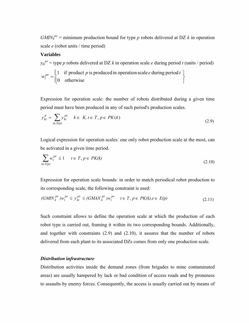
GMINkpe = minimum production bound for type p robots delivered at DZ k in operation
scale e (robot units / time period)
Variables
yktpe = type p robots delivered at DZ k in operation scale e during period t (units / period)
otherwise0
periodduringscaleoperation in producedisproductif1 tepw pe
t
Expression for operation scale: the number of robots distributed during a given time
period must have been produced in any of such period's production scales.
)(, kPKpTt K,kyyE(p)e
pekt
pkt
(2.9)
Logical expression for operation scales: one only robot production scale at the most, can
be activated in a given time period.
PK(k)pTtwE(p)e
pet
,1 (2.10)
Expression for operation scale bounds: in order to match periodical robot production to
its corresponding scale, the following constraint is used:
E(p)PK(k),epTt)w(GMAXy)w(GMIN pet
pek
pekt
pet
pek , (2.11)
Such constraint allows to define the operation scale at which the production of each
robot type is carried out, framing it within its two corresponding bounds. Additionally,
and together with constraints (2.9) and (2.10), it assures that the number of robots
delivered from each plant to its associated DZs comes from only one production scale.
Distribution infrastructure
Distribution activities inside the demand zones (from brigades to mine contaminated
areas) are usually hampered by lack or bad condition of access roads and by proneness
to assaults by enemy forces. Consequently, the access is usually carried out by means of

helicopters. Those aspects of the supply chain that are related to delivery into DZs are
very important due to expensiveness of helicopter fleet operation and buying cost. The
helicopter fleet size can be obtained by means of the following expression:
Variables
HMAXx = minimum number of helicopters used at DZ k in the planning horizon (units)
Expression for helicopter fleet minimum size
TtKkHHMAX ktk , (2.12)
The helicopter fleet minimum size at each DZ corresponds to the maximum number of
helicopters used during a given time period within the studied planning horizon.
Some other considerations about supply chain capacity
As it has been shown, in studying the previous aspects, certain relevant capacity
constraints were added to the supply chain model. Nevertheless, it is necessary to
include some additional capacity considerations. Two relevant constraints are
respectively associated to throughput production capacity due to raw material
procurement bounds, and to the necessary infrastructure to carry out the distribution
process from plants to DCs and within the DZs.
Sets
I : suppliers
PJK(j,k) : robot types delivered from plant j to DZ k.
Parameters
HEk = number of available helicopters in DZ k
XMAXjkp = distribution capacity for type p robot from plant j to DZ k in the planning
horizon (units / period)
ZMAXk = maximum number of feasible helicopter trips in DZ k
βp = helicopter pay load capacity for transporting type p robots (robot units / helicopter)

Variables
Hkt = number of helicopters used at DZ k during period t (units / time period
zkt = number of helicopter trips at DZ k during period t (trips / period)
Expression for distribution capacity bounds, due to supply channel capacity:
jiAIJaTtiJIjIiSMAXyqSMIN a
ijKJk aiPIAp
pkt
apai ,,,,
,
(2.13)
The raw material used for a certain product must be adjusted within the raw material
procurement bounds established by each supplier.
Expression for distribution capacity from plants to DCs:
kjPJKpTtKkJjXMAXy pjk
pkt ,,,, (2.14)
The above constraint takes into account the distribution capacity between plants and
DCs.
Expression for distribution capacity within DZs:
PpTtKkHzy ktktpp
kt ,, (2.15)
The above constraint contemplates both payload capacity and operational frequency of
helicopter trips within DZs.
Expression for maximum number (maximum bound) of helicopters within DZs:
TtKkHEH kkt , (2.16)
Expression for maximum number (maximum bound) of helicopter trips per time period
within DZs:

TtKkZMAXz kkt , (2.17)
Demand
Data collected by the local observatory will allow the classification of an area as
contaminated by mines. The consequent demand for robots is not determined by the
number of mines to be detected, but the extension of the contaminated area, due to the
fact that if a specific land strip is contaminated, then it has to be entirely scanned by
robots, in disregard of how many mines it might have.
As for the robots, it has to be taken into account that a percentage of them will
periodically be rendered useless. Additionally, when considering a Demand Zone (DZ),
the model assumes a stochastic contaminated area which is scanned by robots, where
each robot type has an average scanning speed defined for each period. In order to
suitably model the stochastic area, chance constraints are included [Charnes and Cooper,
1959]; but this requires a certain level of compliance probability for each given
constraint. The associated constraint (eq 2.16) is shown below:
Parameters
α = significance level
θ p = type p robot expected scanning speed in a given planning period (scanned area
units / robot)
φp = expected contingent fraction of type p robots in a given planning period (percentage
/ period)
πp = type p robot estimated operational life span (time units)
Θk(ξ) = mine contaminated stochastic area in DZ k in the planning horizon (area units)
Chance constraint for DZ stochastic area robotic de-mining in the planning horizon
KkwywyP kPp pEe l
pe
lNk
p
lNk
ppppekt
pkt
ppN
t
p
p
pp
p
l
1)()(
1
01,1,
1(2.18)

The above constraints express the minimum permissible target probability required to
scan the mine contaminated area in the planning horizon.
Variable bounds
AaJjIis aij ,,0
)(,,0 kPKpKkJjx pjk
kPKpKkd pk ,0
integerand,,0 kPKpTtKky pkt
integerand,,,0 pEekPKpTtKky pekt
integerand,0 TtKkzkt
integerand,0 TtKkH kt
integerand,0 TtKkHMAX k (2.19)
Objective function
The planning model has to take into account the fixed costs of a series of supply chain
activities, like construction (installation) and operation of factories and DCs, or logistic
flows of raw materials and manufactured products between suppliers, plants, and DZs.
In sum, the fixed costs of the procurement, production and distribution stages.
Additionally, the model not only considers certain fixed costs (e.g., infrastructure) that
can be estimated by assigning them a constant value along the entire planning horizon,
but also those that go through periodical changes (like production and distribution), and
are equally included in the planning horizon. Finally, the model follows Silver and
Perterson’s proposal (1985) of inventory quantification, which includes safety stock
factors, lead times, and inventory cycle factors. The proposal assumes that stochastic
demand and deterministic lead times are independent for each raw material.
Sets
P : robot types

Parameters
Fija = type a raw material inter arrival time from supplier i to plant j (time units /
planning horizon)
Fjkp = type p robot inter arrival time between plant j and DZ k (time units / planning
horizon)
FCI = inventory cycle factor (percentage)
FISja = safety stock factor for type a raw material at plant j (time units / planning
horizon)
FISkp = type p robot safety stock factor at DZ k (time units / planning horizon)
H = holding cost ($ / $ planning period)
Lija = expected lead time for delivering raw material from supplier i to plant j
Ljkp = expected lead time for delivering type p robots from plant j to DZ k (time / raw
material)
Costs:
Cia = procurement cost of raw material a provided by supplier i (including transportation
and duties) ($ / robot)
Ckp = distribution cost of type p robots employed at DZ k (including transportation and
duties) ($ / robot)
Cjkp = cost of type p robot distribution from plant j to DZ k ($ / period)
Cktpe = production cost of type p robots used in DZ k in operation scale e during period t
($ / robot)
CCkt = fuel costs at DZ k in period t ($ / helicopter trip)
CFj = fixed cost of factory j ($/ planning horizon)
CFk = operation fixed cost for DZ k ($ planning horizon)
CH = helicopter cost ($ / helicopter)
CHkt = helicopter operation fixed cost at DZ k during period t ($/period)
CIja = raw material a inventory cost at production site j ($ / planning horizon)
CIkp = type p robot inventory cost at DZ k ($ / period)
CMp = type p robot maintenance cost ($ / robot)

Kkk
Kk Ttktkt
Kk Tt Pp pEe
pet
pkt
pp
KJ(j)k k)PJK(jp
pjk
pjp
ak
pjk
pjk
pk
Kk Pp
pk
pk
JI(i)j j)AIJ(ia
aij
aij
aj
aij
aij
aj
iJIj jiAIJa
aij
ai
Kk Tt kPKp pEe
pet
pkt
pekt
Iiij
Kk Ttktkt
Kkk
CFzCCwyCM
xLFISFFCILHCINdCN
sLFISFFCILHCINsCN
wyCACFHCHHMAXCHMIN
)()1(
)()(
)(
,
,,
)(
(2.20)
2.4. Solution Procedure 1
The design of the supply chain model was based on conceiving the strategic aspects in a
single time period (the planning horizon) and the tactical ones in all periods of the
temporary horizon, therefore having respect for the specific nature of both types of
decision. The following steps are suggested in order to obtain an MIP model, which is
used as an approximation of an MINLP one:
Step 1: approximation to non-linearity
With respect to non-linear constraints, those related to distribution capacity by means of
helicopters at DZs (2.15), procurement reliability (2.1) and stochastic demand area
(2.18) are treated here. First of all, the variables associated to helicopter distribution
capacity constraints had to be redefined. In the case of the reliability constraint (2.1),
logarithmic and absolute value function properties are used. With regards to the
stochastic area expression (2.18), a Gaussian area is assumed and then a deterministic
approximation of such constraint is obtained. In conclusion, as a result of step 1, a less
complex problem is obtained, as shown next:
▪ As for helicopter distribution constraints, given that:
integerandTtKkHz ktktkt , (2.21)
and replacing that expression in eq. (2.15), we have:

TtKky ktpp
kt , (2.22)
Expression for maximum number of periodic distribution trips per fleet at DZ:
TtKkHZMAXHEzMIN ktkkktkt ,, (2.23)
▪ The procurement reliability constraint (2.1) is in turn replaced by the following
equivalent:
jPJpJjPROPROBv p
jjIJi jiAIJa
aij
aij
,)ln()ln(,
(2.24)
In order to deal with the non-linearity associated to the product of the continuum and
binary variables, the approximation suggested by Hanson and Martin (1990) is applied,
including variable redefinition and incorporating additional constraints. The procedure is
carried out as follows:
Assuming that product � x � appears in the model, where � is a binary variable {0.1},
while � is a continuous non-negative variable, then the following procedure can be
carried out:
ΩΔ
ΞMΞΔ
ΩMΞΩΔ )1( (2.25)
where:
MΩ : maximum bound of �, corresponding to a positive integer parameter
MΞ : maximum bound of product � x �, corresponding to a positive integer parameter
The transformation can be used to approximate the non-linearity of equations (2.20) and
(2.4). As a consequence, the following variables are defined and substituted in the
aforementioned constraints:
E(p)ePK(k),pT,tK,kwy pet
pkt
pekt (2.26)

k)PJK(jpK,kJ,jdBx pkjk
pjk , (2.27)
Finally, the following constraints are incorporated to the suggested model
E(p)ePK(k),pT,tK,ky pkt
pekt (2.28)
E(p)ePK(k),pT,tK,kwGMAX pet
pek
pekt (2.29)
E(p)ePK(k),pT,tK,kMwy pet
pkt
pekt )1( (2.30)
k)PJK(jpK,kJ,jdx pk
pjk , (2.31)
k)PJK(jpK,kJ,jBEzx jkkkpjk ,)()(1 (2.32)
k)PJK(jpK,kJjMBdx jkpk
pjk ,)1( (2.33)
The stochastic demand constraint (2.18) is replaced by the expression below (the
corresponding procedure is presented in the Appendix A). In consequence, the stochastic
area in the mentioned equation is simplified into a Gaussian distribution, which is a
commonly encountered condition in practical cases
Kk
Ezl kkPp pEe l
pelNk
ppppekt
ppN
t
p
p
p
p
)()(1
)(
1
01,
1
(2.34)
Step 2: Acquisition of valid constraints
The minimum and maximum objective bounds of the supply chain are obtained by
means of a procedure that stipulates a single production scale range, containing two
linear problems to be solved. In the first (second) one, the minimum (maximum) bound,
is obtained by determining the maximum (minimum) scale cost for each factory-robot-
period combination.
For both models, the associated procedure goes as follows: in the first place, each DZ's
product flow bounds are established:
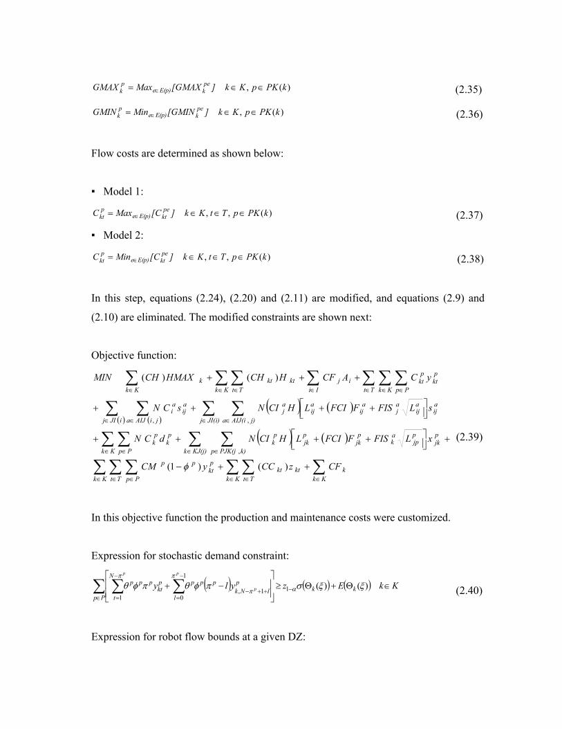
)(, kPKpKk][GMAXMaxGMAX pekE(p)e
pk (2.35)
)(, kPKpKk][GMINMinGMIN pekE(p)e
pk (2.36)
Flow costs are determined as shown below:
▪ Model 1:
)(,, kPKpTtKk][CMaxC pektE(p)e
pkt (2.37)
▪ Model 2:
)(,, kPKpTtKk][CMinC pektE(p)e
pkt (2.38)
In this step, equations (2.24), (2.20) and (2.11) are modified, and equations (2.9) and
(2.10) are eliminated. The modified constraints are shown next:
Objective function:
Kkk
Kk Ttktkt
Kk Tt Pp
pkt
pp
KJ(j)k k)PJK(jp
pjk
pjp
ak
pjk
pjk
pk
Kk Pp
pk
pk
JI(i)j j)AIJ(ia
aij
aij
aj
aij
aij
aj
iJIj jiAIJa
aij
ai
Tt Kk Pp
pkt
pkt
Iiij
Kk Ttktkt
Kkk
CFzCCyCM
xLFISFFCILHCINdCN
sLFISFFCILHCINsCN
yCACFHCHHMAXCHMIN
)()1(
)()(
,
,,
(2.39)
In this objective function the production and maintenance costs were customized.
Expression for stochastic demand constraint:
KkEzyly kkPp l
plNk
ppppkt
ppN
t
p
p
p
p
)()(1
1
01,
1
(2.40)
Expression for robot flow bounds at a given DZ:

PK(k)pTt K,kGMAXyGMIN pk
pkt
pk , (2.41)
Once the problems are solved, the objective function bounds can be determined
Minimum bound –OFMIN–: Min {Model 1}
Maximum bound –OFMAX–: Min {Model 2}
The valid constraint obtained is incorporated to the original model and presented below:
OFMAXCFzCCCM
xLFISFFCILHCINdNC
sLFISFFCILHCINsNC
CACFHCHHMAXCHOFMIN
Kkk
Kk Ttktkt
Kk Tt Pp pEe
pekt
pp
KJ(j)k k)PJK(jp
pjk
pjp
ak
pjk
pjk
pk
Kk Pp
pk
pk
JI(i)j j)AIJ(ia
aij
aij
aj
aij
aij
aj
iJIj jiAIJa
aij
ai
Kk Tt Pp pEe
pekt
pekt
Iiij
Kk Ttktkt
Kkk
)()1(
)()(
)(
,
,,
)(
(2.42)
Summarizing, it can be said that, as a result of the solution procedure, an MIP (and
therefore a more treatable) formulation of the original problem is attained. Such
formulation is made up of equations: 2.2, 2.3, 2.5 to 2.14, 2.16, 2.17, 2.19, 2.22 to 2.24,
2.28 to 2.34, and equation 2.42, together with its associated objective function
2.5. Solution Procedure 2
If the production scale constraints (eq: 2.9, 2.10 and 2.11) are not directly included in the
MNMIP model, but are contemplated later, once the new relaxed MIP problem has been
solved, a new solution procedure can be obtained, as presented next.
Step 1: solving the relaxed MIP problem: the solution of the problem is expressed by
constraints (equations) 2.2, 2.3, 2.5 to 2.8, 2.12 to 2.14, 2.16, 2.17, 2.19, 2.22 to 2.24,
2.31 to 2.34, 2.40, 2.41, and a modified objective function (eq. 2.39) from which the
production cost has been removed, as shown below:
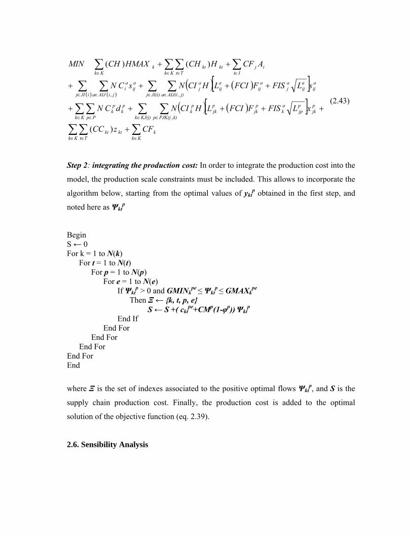
Kkk
Kk Ttktkt
KJ(j)k k)PJK(jp
pjk
pjp
ak
pjk
pjk
pk
Kk Pp
pk
pk
JI(i)j j)AIJ(ia
aij
aij
aj
aij
aij
aj
iJIj jiAIJa
aij
ai
Iiij
Kk Ttktkt
Kkk
CFzCC
xLFISFFCILHCINdCN
sLFISFFCILHCINsCN
ACFHCHHMAXCHMIN
)(
)()(
,
,,
(2.43)
Step 2: integrating the production cost: In order to integrate the production cost into the
model, the production scale constraints must be included. This allows to incorporate the
algorithm below, starting from the optimal values of yktp obtained in the first step, and
noted here as Ψktp
BeginS ← 0For k = 1 to N(k) For t = 1 to N(t) For p = 1 to N(p) For e = 1 to N(e) If Ψkt
p > 0 and GMINkpe ≤ Ψkt
p ≤ GMAXkpe
Then Ξ ← {k, t, p, e} S ← S +( ckt
pe+CMp(1-φp)) Ψktp
End If End For End For End ForEnd ForEnd
where Ξ is the set of indexes associated to the positive optimal flows Ψktp, and S is the
supply chain production cost. Finally, the production cost is added to the optimal
solution of the objective function (eq. 2.39).
2.6. Sensibility Analysis

The sensibility analysis was performed using solution procedure 1, with the aid of a
commercial LINGO 10™ software package. The computing of the scenarios was carried
out on a Pentium-4 2.8 Ghz, 1GB RAM equipment, applying a Win XP-SP2 operational
program. The problem comprises 20 suppliers handling 2 components each, 10 possible
plant locations, 2 products in two production scales, and 20 Gaussian DZs. All possible
combinations of logistic procurement connections were admitted, together with a
distribution network featuring three DCs per production plant. Finally, a 5% Gaussian
significance was used for the demand chance constraint. These problems have 14048
constraints and 4171 variables, of which 1241 are binary. The parameters under scrutiny
were: area size, helicopter capacity and robot speed performance. Instance solutions take
500 seconds in average, with a maximum of 900 seconds. All the program runs were
conducted with a maximum gap of 0.001, and most of the results were probably optimal.
The following table presents the percentage ranking of the average unitary costs that are
part of the objective function:
Table 2.1: Average unitary cost percentage structure of the supply chain
CHkt CFj Cktpe Ci
a CIja Ck
p CIkp CMp CCk
t
64 35.62 0,0725 0.0534 0,0312 0,0044 0,04025 0,05 0,0001
As it can be observed, the highest average unitary costs correspond to the strategic
aspects, which are infrastructure distribution, and plant and distribution centre
installation.
The sensibility analysis is applied by modifying the parameter percentage values and
monitoring their impacts on the total cost of the supply chain.
Demand effect on minimum cost
Although the costs rise in direct relation to the expansion of the demand area, the non-
linear nature of the problem becomes evident when changes in production scale and

distribution infrastructure occur (e.g. more helicopters are required in order to satisfy a
greater demand for robots). The smooth behaviour of the costs in some sections of
Figure 2.1 is due to tactical changes in the supply chain. The slope remains unchanged
as long as no adjustments in production or distribution infrastructure are undertaken in
order to satisfy the demand, as can be observed in Figure 2.1.
0%
5%
10%
15%
20%
25%
-50% -40% -30% -20% -10% 0% 10% 20% 30% 40% 50%
% Demand Change
% C
han
ge M
inim
un
Co
st
Figure 2.1: Effect of demand on minimum cost
Effect of robot scanning speed on minimum cost
Robot scanning speed appears to be the most influential cost factor, since it constitutes
the link between inventory, production and distribution activities in both strategic and
tactical contexts. On the one hand, the costs associated to production and distribution,
diminish as scanning speed increases. On the other hand, inventory costs rise when there
is an increasing number of unused robots during long time periods, as a consequence of
the scanning speed increase. These two tendencies determine a general behaviour,
according to which there is an overall cost percentage drop, marginally decreasing as the
scanning speed is raised, due to the existence of counter-balance costs within the same
objective function. (See figure 2.2).

0%
5%
10%
15%
20%
25%
-40% -30% -20% -10% 0% 10% 20% 30% 40%
% Scan Speed Change
% C
han
ge M
inim
un C
ost
Figure 2.2: Effect of robot scanning speed on minimum cost
Effect of helicopter capacity on minimum cost
Due to the fact that helicopters offer multiple usage possibilities, it is important to
analyze their potential payload percentage per trip. As shown in Figure 2.3, helicopter
payload capacity has a significant impact on distribution costs, and therefore, on overall
costs. Variation in total costs as a result of changes in helicopter payload capacity is
similar to that shown in Figure 2.2, resulting from robot scanning speed, as far as both
parameters have a similar effect on distribution costs at DZs.
0%
2%
4%
6%
8%
10%
12%
-40% -30% -20% -10% 0% 10% 20% 30% 40% 50%
% Helicopter Capacity Change
% C
han
ge
Min
imu
n C
ost
Figure 2.3: Effect of helicopter capacity on minimum cost

2.7. Conclusions
The current paper presents an MIP and an MNMIP models for anti-personal landmine
disposal by means of robots that – following the recommendations found in the cited
references - include and integrate strategic and tactical relevant aspects of the supply
chain. For that reason the model includes certain considerations, such as uncertain
procurement, stochastic inventories in plants, production scales, supply-production-
distribution capacities, particular distribution-production infrastructure, location-
allocation considerations, stochastic demand, and BOM. Additionally, the models detail
optimal helicopter operation by considering each period's trip frequency during the
planning horizon.
For their solution, two procedures are suggested, allowing to convert the original (and
relatively hard) MINLP into a not so hard MIP. The efficiency of the second procedure
tends to improve when the operation scales are considerable enough; otherwise, it
lessens. On the other hand, the first procedure is advantageously explicit, in contrast
with the second one, where the production cost is algorithmically induced.
Finally, the impact of parameter percentage variations on the overall cost is analyzed.
The costs do not substantially differ if percentage variations do not entail changes in
plant operation level or in the number of helicopters used in the distribution. The
suggested solution procedure is considered satisfactory in terms of time for the analyzed
example.
Some of the research perspectives comprise qualitative aspects, while some other
comprise quantitative aspects, all of them potentially relevant for the decision making
process under more specific contexts.
2.8. References
Aikens, C.H. (1985), Facility location models for distribution planning. European
Journal of Operational Research. 22 263-279.

Arntzen, B.C., Brintegrated, G.G., Harrison, T.P., Trafton, L.L. (1995), Global supply
chain management at digital equipment corporation. Interfaces 25 (1) 69-93.
Charnes, A., Cooper, W.W. (1959), Chance- constrained programming. Management
Sciences 5, 73-79.
Chen, C., Lee, W. (2004), Multi-objective optimization of multi-echelon supply chain
networks with uncertain product demands and prices. Computers & Chemical
Engineering 28 1131 – 1144.
Cohen, M.A., Lee, H.L. (1988), Strategic analysis of integrated production-distribution
systems: Models and methods. Operations Research 36 216-228.
Geoffrion, A.M., Graves, G. (1974), Multicommodity distribution system design by
Benders decomposition, Management Science 20(5) 822- 844.
Geoffrion, A.M., Powers, R.F. (1995), Twenty years of strategic distribution system
design: An evolutionary perspective. Interfaces 25 105-127.
Goetschalckx, M., Vidal, C.J., Dogan, K. (2002), Modeling and design of global logistic
system: A review of integrated strategic and tactical models and design algorithms.
European Journal of Operational Research 143 (1) 1-18.
Gupta, A., Maranas, C.D. (2003), Managing demand uncertain in supply chain planning.
Computers & Chemical Engineering 27 1219 – 1227.
Hanson, W., Martin, R.K. (1990), Optimal Bundle Pricing. Management Science 36 (2)
155 – 174.
Landmine Monitor Report : Toward a Mine-Free World. 2003.
Silver, E.R., Peterson, R. (1985), Decision systems for inventory management and
production planning, second ed., New York.
Thomas, D., Griffin, M.C. (1996), Coordinate supply chain management. European
Journal of Operational Research 94 1-15.
Vidal, C.J., Goetschalckx, M. (1997), Strategic production-distribution models: A
critical review with emphasis on global supply chain models. European Journal of
Operational Research, 98 1-18.
Vidal, C.J., Goetschalckx, M. (2001), Modeling the effect of uncertainties on global
logistics systems. Journal of business logistics, 21 (1) 95-120.

2.9. Appendix A
The chance approximation of the stochastic demand constraint is presented in the
following equation:
Kk
wylwyP kPp pEe l
pelNk
plNk
ppppekt
pkt
ppN
t
p
p
pp
p
1)()(
1
01,1,
1 (A1)
Kk
EwylwyEA
Pk
Ppk
pEe l
pelNk
plNk
ppppekt
pkt
ppN
t
p
k
kk
p
pp
p
1)(
)(
)(
)()( )(
1
01,1,
1
(A2)
Kk
Ewylwy
k
Ppk
pEe l
pelNk
plNk
ppppekt
pkt
ppN
t
p
p
pp
p
F
1)(
)()(
1
01,1,
1
(A3)
Under the normal demand assumption
Kkz
Ewylwy
k
Ppk
pEe l
pelNk
plNk
ppppekt
pkt
ppN
t
p
p
pp
p
1)(
1
01,1,
1
)(
)(
(A4)
The following is an approximate deterministic constraint of equation (A1).
Kk
Ezwylwy kkPp pEe l
pelNk
plNk
ppppekt
pkt
ppN
t
p
p
pp
p
)()(1
)(
1
01,1,
1
(A5)

CHAPTER THREE
Send to Cuadernos de Economía: Latinoamerican Journal of Economics
Status: Publicated: v.44, (Noviembre), p.233 - 262, 2007.

Costos de Transacción y Formas de Gobernación de los Servicios de
Consulta en Colombia: un estudio empírico
Sergio Torres Valdivieso*
Rafael Guillermo García Cáceres **
John Jairo Quintero***
Abstract
The present paper considers the extent to which the establishment of the different
governance forms linking hospitals to insurance companies in Bogotá, is carried out
taking into account transaction costs reduction criteria. An empirical test is applied,
making use of the transaction dimensions proposed by Williamson (1985). Hypotheses
are tested by means of a combination of the stochastic multicriteria acceptability
analysis, and multiple discriminant analysis. It is concluded that both hospitals and
insurance companies seek to reduce production costs, while transaction costs are not
relevant to the decision.
Palabras clave: Criterios de decisión, Organización Industrial, Costos de transacción
Aplicaciones en sector salud.
JEL classification: D810, L000, D230
3.1. Introducción
Con la promulgación de la Ley 100 de 1993, se reemplaza el Sistema Nacional de Salud,
que venía operando en Colombia desde 1973, por el Sistema General de Seguridad
Social en Salud –SGSSS-. Uno de los objetivos que se buscaba con la implantación del
SGSSS es el aumento de la eficiencia del sistema, para lo cual se introdujeron las
siguientes modificaciones: i. se separaron las funciones de aseguramiento y prestación
Este artículo es producto de la investigación “Análisis del Impacto de las Formas de Contratación entre Prestadoras y Administradoras de Salud, sobre los Costos de transacción para las Prestadoras de Servicios de Salud de III Nivel de Atención”, la cual a su vez es parte del Proyecto “Optimización de los Elementos Estratégicos de la Cadena de Abastecimiento, Bajo una Perspectiva de los Costos de Transacción: Caso de Medicamentos En Bogotá.”, financiado por Colciencias y la Pontificia Universidad Javeriana.Email: *[email protected], **[email protected], ***[email protected].

de servicios de salud y se permitió la participación del sector privado; ii. la relación
entre aseguradores y prestadores está dada por el modelo de competencia regulada
propuesta por Enthoven (1997) en el cual el estado juega fundamentalmente el papel de
regulador. Estas ideas las retoman Londoño y Frenk (1997) para el planteamiento de este
tipo de reformas en América Latina.
En este contexto está claramente reconocida la importancia de estudiar los sistemas de pago
y formas de contratación de los servicios de salud en Colombia, debido al efecto que éstos
tienen sobre la calidad de los servicios y el desarrollo tecnológico del sector [Gutiérrez, et
al., 1995; Álvarez et al., 2000]. Sin embargo, en los estudios realizados esta visión no se
amplía a la comprensión de las formas de gobernación, que contemplan tanto sistemas de
pago como formas de contratación. Este aspecto ha sido poco estudiado en el sector salud
en Colombia, lo que justifica la realización de esta investigación. El estudio de las formas
de gobernación de la consulta externa es parte de un conjunto de trabajos que exploran los
diversos tipos de servicios de salud como son los servicios de urgencias y la cirugía
programada, los cuales difieren entre sí.
Las investigaciones sobre formas de gobernación del intercambio económico de bienes y
servicios se han basado teóricamente en la economía de costos de transacción,
perspectiva de las capacidades organizacionales y la estrategia y referentes sociológicos
como la teoría institucional o la teoría contingente [Pisano, 1988; Mang, 1994; Lewin y
Volverda, 1999; Torres, 2003]. Este estudio de carácter exploratorio tiene como objetivo
estudiar las formas de contratación de los servicios de consulta externa en las IPS
privadas de tercer nivel de atención en Bogotá desde la Economía de los Costos de
Transacción, debido a que es el referente fundamental para explicar la forma en que se
organiza el sistema económico [Williamson, 1975, 1985, 1991].
La presentación del estudio está organizada de la siguiente forma. En la primera parte
del artículo se presentan los principales rasgos de funcionamiento del Sistema General
de Seguridad Social en Salud en Colombia y algunos aspectos distintivos de la

prestación de servicios de consulta externa. En la segunda parte, se hace una exposición
sobre la economía de los costos de transacción y las hipótesis de allí derivadas. Le sigue
la metodología de investigación, en que se presenta el plan de análisis mediante dos
técnicas matemáticas complementarias. En el siguiente numeral se exponen los
resultados de la investigación y se finaliza con la discusión de los mismos.
3.2. Elementos del contexto de los Servicios de Consulta Externa
3.2.1 Legislación sobre las formas de contratación y pago en el Régimen Contributivo
En Colombia se hace referencia a las formas de pago y no a las formas de gobernación.
En las referencias sobre formas de pago en Colombia los mecanismos más
frecuentemente encontrados en las relaciones entre aseguradores –EPS- y prestadores –
IPS- de servicios de salud son el pago por servicio, pago por paquetes de enfermedades
y pago por capitación [Gutiérrez et al., 1995; Molina, 1995; Torres et al, 2004]. El pago
por servicio se define como el pago realizado por la totalidad de la atención de salud
prestada a un individuo. La remuneración incluye honorarios médicos, suministros,
medicamentos y servicios quirúrgicos. El pago sin embargo, no se puede estipular ex-
ante debido a que la atención depende de los requerimientos de cada paciente y servicio.
El pago por capitación está basado en el concepto de enfermo potencial y no en el de
enfermedad sentida como en el caso anterior. El prestador de servicios tiene a su cargo
la atención de un conjunto determinado de personas. Por cada persona inscrita recibe un
giro periódico de la EPS, sin importar el número de veces que acuda al servicio médico
cada una de las personas capitadas.
El pago por caso es una forma de contratación que contiene elementos de las formas de
pago anteriores. La unidad de medida es el tratamiento global de un tipo de dolencia
específica sobre la que se conocen adecuadamente los protocolos a seguir para su
tratamiento, por lo tanto se conocen adecuadamente los costos de tratamiento.

Teniendo esto como punto de partida, se enuncian los elementos en que la legislación
colombiana se refiere a las relaciones entre IPS y EPS. En primer lugar, en la Ley 100 de
1993 se permite que la forma de gobernación entre EPS e IPS sea la integración vertical.
Aunque una misma persona jurídica no puede ejercer las funciones de aseguramiento y
prestación de servicios de salud, es factible que un mismo grupo empresarial sea
propietario de dos empresas independientes. Por otra parte, atendiendo de forma más
clara el espíritu del pluralismo estructurado sobre el que se construyó el Sistema General
de Seguridad Social en Salud los agentes económicos pueden acudir a dos formas de
gobernación alternas, el mercado para la compra de servicios de salud o establecer
alianzas estratégicas entre organizaciones.
El segundo elemento para comprender la relación entre aseguradores y prestadores de
servicios de salud son las formas de pago. La legislación emitida sobre formas de pago
no es muy amplia y se refiere de forma independiente al Régimen Contributivo y el
Régimen Subsidiado. Respecto al pago por servicios prestados, el primer referente está
en el Decreto 2423 de 1996 en el cual se establecen tarifas, nomenclatura y clasificación
de los procedimientos médicos, quirúrgicos y hospitalarios que se intercambian entre los
aseguradores de los servicios de salud y las IPS públicas y privadas para la atención de
pacientes víctimas de accidentes de tránsito, desastres naturales, atentados terroristas,
atención inicial de urgencias y los demás eventos catastróficos definidos por el Consejo
Nacional de Seguridad Social en Salud. En la práctica este Manual Tarifario funciona
como una referencia que usan aseguradores y prestadores para fijar los precios de
intercambio. Por otra parte, el Decreto 050 de 2003 establece que los pagos a los
prestadores de servicios no pueden tomar más de seis meses desde el momento de
radicación de la cuenta de cobro.
Respecto a la forma de contratación por capitación, el Decreto 050 de 2003 señala las
siguientes condiciones a cumplir: se debe garantizar la adecuada prestación de los
servicios; por esta razón se considera como una práctica insegura contratar a una persona
natural o jurídica para que realice la función de coordinar la red de prestación de

servicios; no se podrá capitar la totalidad de los servicios de más de dos niveles de
atención con la misma IPS, y los pagos a las IPS deben hacerse durante los primeros
diez días de cada mes. Estos son los aspectos que la legislación colombiana tiene en
cuenta para regular las relaciones de contratación entre aseguradores y prestadores.
3.2.2 La consulta externa en los hospitales de tercer nivel
La atención médica en el actual SGSSS de Colombia está establecida según los niveles
de complejidad en la atención, encontrándose tres niveles de atención, siendo el tercer
nivel el de mayor complejidad tecnológica.
El tercer nivel de atención se caracteriza por prestar servicios hospitalarios y
ambulatorios de especialistas en medicina interna, pediatría, ginecología, cirugía general
y ortopedia, entre otras especialidades médicas y quirúrgicas [Malagón et al., 1986], a su
vez cuenta con áreas de urgencias, consulta externa, cirugía, hospitalización y cuidado
intensivo. En síntesis, éste tipo de instituciones atienden los casos de mayor complejidad
médica y tecnológica, lo cual implica la mayor generación de los costos de atención.
La consulta externa se entiende como la actividad alrededor de la que giran los procesos
de especialización médica; siendo el espacio idóneo para diagnosticar, orientar definir la
estrategia terapéutica de un paciente. En la actualidad la consulta externa cobra
importancia en la medida que se torna en la puerta de entrada al sistema, lo que permite
realizar un mayor control de costos. Está claro que se debe dar una interacción entre la
consulta externa de los diferentes niveles de atención.
En Colombia los servicios de consulta externa de los primeros niveles de atención los
realizan las EPS e IPS del primer y segundo nivel de atención, de manera que la consulta
externa del tercer nivel de atención se realiza en IPS del tercer nivel; las cuales, pueden
tener diversas formas de interacción con las EPS y con las IPS de primero y segundo
nivel de atención [Gorbaneff et al., 2004].

3.3. Marco Teórico
Los problemas fundamentales que estudia la economía y que enfrentan las
organizaciones en su vida cotidiana son la producción e intercambio de bienes y
servicios. Desde el punto de vista de la organización de la actividad económica, las
personas involucradas en las actividades productivas pueden solucionar estos problemas
acudiendo a tres tipos de formas de gobernación [Williamson, 1991; Li, 1998; Hage y
Alter, 1997]: el mercado, la integración vertical de diversos agentes económicos en una
estructura jerárquica que toma la denominación de empresa y el establecimiento de
relaciones de cooperación entre agentes usualmente llamadas alianzas estratégicas. Entre
estos tres tipos ideales [Doty y Glick, 1994] de realización del intercambio económico se
pueden encontrar formas más complejas que son producto de la mezcla de las
características fundamentales de los tipos ideales señalados [Torres et al., 2004].
Las formas de gobernación genéricas establecidas en la economía de costos de
transacción tienen vigencia en el sector salud y particularmente en las relaciones de
intercambio que establecen las EPS e IPS. Con el fin de unificar los términos se hablará
de tres (3) formas de gobernación: integración vertical, alianzas estratégicas y mercado
(ver Tabla 3.1).
Es necesario hacer una mención especial sobre los incentivos económicos. Estos van a
estar dados por la forma de gobernación del intercambio y por el sistema de pago que se
use. El tipo de contrato determina la intensidad de los incentivos del agente, siendo bajos
cuando hay un contrato de empleó como es típico en la integración vertical. Por otra
parte, los incentivos se aumentan hasta llegar a su máxima expresión cuando la
propiedad es individual.
Sobre las formas de pago, se debe tener claro que se pueden presentar diversas formas
bajo la misma forma de gobernación. La forma de pago lo que hace es cambiar el
aspecto de la transacción en el que se colocan los incentivos y la distribución del riesgo
entre las partes [Seshadri, 2005]. En la forma de pago por capitación todo el riesgo es

asumido por el agente y le genera un incentivo a la reducción de costos. En el pago por
servicio el riesgo lo asume parcialmente el principal y el agente tiene un incentivo fuerte
a la facturación.
En un intercambio de mercado se puede usar cualquier forma de gobernación con altos
incentivos pero dirigidos de diferentes formas. En las alianzas estratégicas se pueden
usar las tres formas de pago, pero el riesgo se distribuye entre las partes. Finalmente, en
la integración vertical por definición el riesgo lo asume el principal y el agente tiene
bajos incentivos.
Sobre las formas de pago es necesario hacer una aclaración. El pago por capitación
implica que el intercambio no puede ser de tipo “spot”, como consecuencia el
intercambio de mercado tendrá un horizonte de mediano plazo; en tanto, el pago por
servicios es más característico del mercado “spot”.
Tabla 3.1. Dimensiones de las Formas de Gobernación del Intercambio en el Sector Salud
Fuente: Adaptado de Torres et al., (2004).
Formas de GobernaciónAtributos
Integración Vertical Alianzas estratégicas Mercado
Formas de interacción Mandato Acción conjunta Competencia
Mecanismos de control Planeación Confianza Sistema de precios
Marco Legal Laboral Amplio Específico
Propiedad Unificada (bajos) Compartida (Intermedios) Individual (altos)
Capitació
nBajos
Altos para ahorrar bajo
acuerdos de calidad
Altos para ahorrar
Pago por
paquetes Intermedios
Altos para vender
paquetes y altos para
ahorrar dentro del paquete
Incentivos
Económicos
For
mas
de
pago
Pago por
servicio
Altos para gastar bajo
acuerdos de control de
costos
Altos para gastar

Como se ha mostrado, la única opción posible para realizar el intercambio de bienes y
servicios no es el mercado, sino que los agentes pueden acudir a la creación de empresas
y de alianzas estratégicas, ¿de qué depende esta decisión?. Siguiendo la propuesta
teórica de Coase (1937) y Williamson (1975, 1985, 1991), los agentes que buscan
racionalidad económica, mediante la selección de la forma de gobernación de realizar el
intercambio, buscan reducir la suma de los costos de producción y los costos de
transacción.
Los costos de producción están asociados a las actividades productivas directas y se
encuentran representados por los diversos recursos requeridos para la prestación de los
bienes o servicios, tales como el trabajo requerido para la producción, maquinaria y
equipo y materias primas. Los costos de producción están determinados
fundamentalmente por el tipo de tecnología disponible, ya que ésta además de establecer
los costos de maquinaria y equipo afectan también los requerimientos de mano de obra.
Si los agentes económicos seleccionasen las formas de intercambio en función de los
costos de producción, se integrarían verticalmente cuando su consumo agotase las
economías de escala y acudirían al mercado cuando su consumo fuese pequeño en
relación a las economías de escala disponibles [Williamson, 1975].
Por otra parte, los costos de transacción se derivan de las actividades que están
relacionadas con la búsqueda y transmisión de información sobre precios y
características de los bienes, negociación de condiciones de intercambio, redacción y
celebración de contratos, supervisión de las contrapartes para el cumplimiento de los
contratos, demandas y adaptaciones del mismo y protección de los derechos de
propiedad [Milgrom y Roberts, 1993]. Las actividades referidas como generadoras de
costos de transacción tienen una doble naturaleza, contractual, y organizacional; las
cuales en conjunto explican los problemas que se presentan en el intercambio mediante
las formas de gobernación.

Como se puede ver los costos de transacción no tienen relación directa con los costos
productivos, para explicar mejor su naturaleza es adecuada la analogía que hace Arrow
(1962) al compararlos con la fricción de los sistemas mecánicos, del tal forma que son
indeseables pero al mismo tiempo inevitables. Como ocurre con los fluidos que las
pérdidas friccionales dependen de su viscosidad, en la organización económica los
costos de transacción dependen de las características de los bienes que se intercambian.
Las características de los bienes o dimensiones de la transacción que determinan los
costos de transacción son: especificidad de las inversiones, dificultades de medición de
los procesos y resultados, frecuencia de la transacción, incertidumbre en la prestación de
los servicios [Williamson, 1991] y relaciones entre las transacciones [Milgrom y
Roberts, 1993].
Como se dijo anteriormente, todas las formas de gobernación generan costos de
transacción, pero estos dependen de las dimensiones de la transacción. Para la
identificación de cual es la forma de gobernación que genera menores costos de
transacción se debe dar una alineación entre las dimensiones de las formas de
gobernación y las dimensiones de la transacción.
Williamson (1985) afirma que la dimensión que explica la mayor parte de los costos de
transacción es la especificidad de las inversiones, definida para este caso como aquella
situación en la que los recursos involucrados en la prestación de los servicios de salud
son solamente útiles para la prestación de servicios a una EPS, lo que generaría una
dependencia bilateral entre las partes. Estas inversiones que son de utilidad únicamente
entre estos dos agentes, generan cuasirentas compuestas [Hart, 1991], que las partes
involucradas buscarán apropiarse mediante comportamientos oportunistas [Pisano,
1988].
En esta situación de dependencia bilateral, entre el aseguramiento y la prestación de
servicios, sí el intercambio se realiza a través del mercado se generarán altos costos de
transacción, fundamentalmente de tipo contractual. Tales costos, se derivan de las

continuas renegociaciones y adaptaciones del contrato a las nuevas condiciones, las
cuales es necesario realizar en la medida que surgen contingencias que desajustan los
términos iniciales de los contratos [Williamson, 1991].
La forma en que se desajusta intencionadamente el contrato inicial, es mediante argucias
como la revelación incompleta de las características epidemiológicas de la población y
de las características de los procedimientos médicos; o mediante la amenaza de
interrupción del contrato u otras acciones que alteran los términos iniciales del
intercambio [Milgrom y Roberts, 1993].
Los riesgos de interrupción prematura de los contratos de prestación de servicios de
salud, los costos contractuales de renegociación de las condiciones iniciales y los costos
burocráticos en que se incurre para la búsqueda de información aumentan en la medida
que los recursos médicos y los resultados de las intervenciones son coespecializados7.
Como alternativa al intercambio de mercado, las organizaciones pueden integrarse
verticalmente, teniendo como resultado la reducción de los costos de adaptación a
circunstancias cambiantes. Esta reducción de costos, es consecuencia de las virtudes de
la integración vertical para coordinar eficientemente situaciones en las que se debe
transmitir información sobre nuevas condiciones y acordar las acciones a realizar
conforme a las contingencias que se han presentado [Williamson, 1991].
La integración vertical reduce los costos de transacción ante altos niveles de
especificidad de las inversiones para la prestación de servicios de salud, reemplazando
los altos costos contractuales por costos burocráticos requeridos para la coordinación y
control de la prestación de servicios. Bajo la forma de propiedad integrada se reducen
los riesgos de terminación prematura del contrato o de desajustes por la revelación
incompleta de información. Lo anterior se resume en la:
7 Los activos coespecializados son aquellos en que hay una dependencia bilateral (Teece, 1986), esto es que los recursos innovadores -I+D, diseño, ingeniería de producción- no son compatibles con los activos complementarios y viceversa.

Hipótesis 1: Existe una relación directa y positiva entre el aumento de la especificidad
de las inversiones y la preferencia por formas de gobernación con mayores niveles de
integración.
Cuando se establecen mecanismos burocráticos especializados para el intercambio de
determinados servicios es necesario realizar esa transacción repetidas veces para poder
recuperar las inversiones. Esta idea acoge el sentido de las economías de escala
propuestas desde la economía neoclásica, para explicar la selección de las formas de
gobernación. El costo de la estructura organizacional se distribuye entre las
transacciones que se realicen, por lo tanto se propone:
Hipótesis 2: Existe una relación directa y positiva en el aumento de la frecuencia y
duración de la transacción y la preferencia por establecer formas de gobernación con
mayores niveles de integración vertical.
Otra fuente de costos de transacción y de especial relevancia en la prestación de
servicios de salud son las dificultades de medición de la actuación de los agentes que
participan en el intercambio de servicios de salud [Milgrom y Roberts, 1993]. Las
dificultades de medición se definen como las limitaciones que tiene la EPS de
supervisar, expost a la elaboración del contrato, el comportamiento de la IPS en la
prestación de los servicios pactados [Barzel, 1989].
Los comportamientos oportunistas derivados de la especificidad de los activos se deben
a la búsqueda de la apropiación de las cuasirentas compuestas mediante el desajuste del
contrato. Ahora bien, cuando confluye la especificidad de los activos con la existencia
de dificultades de medición, el tipo de comportamiento oportunista que surge para
apropiarse de las cuasirentas compuestas, es evadir los compromisos ampliamente
especificados en la fase ex-ante de la contratación del proyecto [Chi, 1994]8. Una
8 Este tipo de oportunismo, expost a la firma del contrato, afecta los resultados y eficiencia de la transacción, ya que las partes deben hacer un esfuerzo mutuo por controlar las acciones del otro, el cual se denomina riesgo moral.

situación agravante es que tan sólo después de finalizada la contratación es posible
detectar el comportamiento anómalo [Alchian y Woodward, 1988].
Si bajo esta circunstancia la contratación se da en el mercado, la empresa innovadora
incurrirá en altos costos de transacción, de una parte, ex-ante, en la recopilación de
información técnica que le permita ser lo más exhaustiva en la determinación de los
resultados de los servicios de salud, y por otra, en costos burocráticos ex-post necesarios
para comprobar la forma en que se prestan los servicios de salud. La situación se debe en
buena medida a que las acciones y resultados de la prestación de servicios de salud no
son tangibles sino que tienen un amplio componente tácito.
El componente tácito en la prestación de los servicios de salud es el aumento de los
costos de transacción y más grave aún el posible deterioro de los servicios de salud.
Ante ésta situación de ineficiencia, tanto productiva como transaccional, la opción de
integración vertical, en que se establecen estructuras burocráticas de control y se
eliminan los incentivos fuertes, permite la reducción de las posibilidades de
comportamientos oportunistas. Estas ideas se sintetizan en la:
Hipótesis 3: En la medida que aumentan las dificultades de medición en la prestación de
servicios de salud se preferirán formas de gobernación con mayor grado de integración
vertical.
Según Williamson (1985), la tercera fuente de costos de transacción es la incertidumbre
en el comportamiento de los agentes que intercambian, en este contexto la incertidumbre
en la prestación de los servicios de salud se entiende como la dificultad posterior a la
contratación, de determinar las acciones y costos en los que deberá incurrir tanto EPS
como IPS en la prestación del servicio de salud. Esta incertidumbre se relaciona en
primer lugar, con las dificultades de predecir el comportamiento de la IPS en cuanto a la
revelación de los costos de prestación de los servicios, y en segundo lugar, con la

posibilidad de la EPS de enviar pacientes con enfermedades en extremo costosas,
cuando la contratación se da vía capitación.
Hipótesis 4: En la medida que aumenta la incertidumbre en la prestación de los
servicios de consulta externa se prefiere realizar el intercambio de servicios mediante
formas de gobernación con mayores niveles de integración vertical.
3.4. Metodología de Investigación
3.4.1 Instrumento y medición
La unidad de análisis de la investigación fue el intercambio de servicios de consulta
externa entre EPS e IPS. Esto porque para la economía de los costos de transacción
[Williamson, 1975, 1985] es en este espacio económico que es posible detectar los
problemas contractuales en el intercambio.
La encuesta se construyó conforme a trabajos previos empíricos que han operado
variables similares a las usadas en esta investigación. Las variables independientes que
conforman el modelo de investigación se midieron con múltiples proposiciones que
reflejan diversas dimensiones del concepto o variable que se desea medir, permitiendo
que los errores en la medición de las afirmaciones se corrijan mutuamente [Churchill,
1979]. Las proposiciones se miden con una escala Likert de 1 a 5, que permite
identificar el nivel de acuerdo o desacuerdo ante una determinada afirmación relativa a
las variables que se indagan [Albaum, 1997]. Es claro que la medida se hace a partir de
una apreciación de la realidad.
Se efectuó una prueba piloto y como resultado se identificaron problemas de
presentación de las preguntas, se efectuaron los ajustes del instrumento de medición, que
posteriormente fue aplicado a la población.
En primer lugar se realizó el análisis de consistencia interna; este análisis evalúa la
confiabilidad del instrumento de recopilación de información y validez de la

información recolectada. La confiabilidad se refiere al grado en que la medición está
libre de error y se determina mediante la correlación entre los indicadores de cada
variable, la correlación corregida y él coeficiente alfa [Nunnally, 1978; Kerlinger, 1986].
La evaluación de la validez de la información se realiza mediante el análisis factorial de
componentes principales [Churchill, 1979]. Esta prueba confirma si los indicadores
seleccionados de una variable están midiendo el mismo fenómeno. Las pruebas de
confiabilidad y validez se realizan de forma iterativa y son típicos cuando se realizan
encuestas con información cualitativa.
En cada variable se realizó un procedimiento de análisis de la consistencia interna de los
indicadores. La evaluación de la confiabilidad del instrumento se inició con el análisis
de correlación no paramétrico de Taub-Kendall. Se usó éste estadístico debido a la
naturaleza no normal de las variables. Luego se efectuaron análisis de correlación
corregida y finalmente se determinó el coeficiente alfa de Cronbach [Nunnally, 1978]; se
considera un alpha aceptable aquel que es mayor a 0,5.
Los análisis de confiabilidad y validez fueron efectuados paralelamente. Los resultados
fueron consistentes, mostrando que los indicadores removidos presentan problemas de
dimensionalidad. Las variables resultantes fueron operadas como factores con el fin de
reducir información que introduce ruido en las variables. Es necesario resaltar la alta
correlación de los indicadores dentro de los factores resultantes, en todos los casos fue
superior a 0,53.
Teniendo en cuenta los aspectos generales descritos se presenta la operación de las
variables relacionadas con las hipótesis planteadas.
Especificidad de las inversiones. Se midió con cinco indicadores relacionados con las
inversiones no recuperables y la posible situación de monopolio bilateral, conforme a los
trabajos de Lothia et al. (1994) y Torres (2003), los indicadores son: dificultades de
reutilización de las inversiones físicas, IPS competidoras en servicios similares, IPS que

podrían desarrollar servicios similares, pérdida de la rentabilidad de las inversiones
físicas si se destinan a otro servicio, y grado en que es necesario modificarlas o
adaptarlas para que puedan ser usadas en otros servicios. La totalidad de los indicadores
fueron consistentes. El coeficiente alpha final es de 0,79. La carga de los indicadores
resultantes en el factor fue de 0,67, 0,77, 0,76, 0,86 y 0,66, respectivamente y el
porcentaje de la varianza extraída por el factor fue de 56,146%.
Frecuencia del intercambio en la prestación del servicio. La frecuencia y duración del
intercambio en los servicios atendiendo a la idea de repetitividad y su duración temporal
se midió con los siguientes indicadores: Frecuencia con la que intercambian servicios de
consulta externa y tiempo durante el cual se ha prestado el servicio entre la EPS y la IPS.
El coeficiente alpha asociado es de 0,54. La carga de los indicadores en el factor fue de
0,83 en los dos casos y el porcentaje de la varianza extraída por el factor fue de 68.5%.
Incertidumbre en la prestación de los servicios. Siguiendo el trabajo de Torres (2003) e
indagando sobre la utilidad de los diversos mecanismos usados para tratar información
sobre la prestación de servicios de salud, se definieron los siguientes indicadores para la
construcción de ésta variable: Dificultades para establecer cláusulas restrictivas en el
contrato, dificultades para el seguimiento de los protocolos de atención o guías de
manejo, complicaciones en el manejo de los pacientes en consulta externa, dificultades
para llevar a buen término el tratamiento de los pacientes y desigualdad en las conductas
tomadas en el servicio. Para aumentar la confiabilidad del instrumento fue necesario
prescindir de los indicadores dificultades para establecer cláusulas restrictivas en el
contrato y desigualdad en las conductas tomadas en el servicio. El coeficiente alpha
calculado es de 0,66. La carga de los indicadores resultantes en el factor es de 0,62, 0,87
y 0,82, respectivamente y el porcentaje de la varianza extraída por el factor fue de
60,4%.
Dificultades de medición de la actuación. Siguiendo los trabajos empíricos de Erramilli
y Rao (1990) y Kim y Hwang (1992), se midió la variable usando cuatro indicadores

para captar el grado de especialización y de estandarización de los conocimientos
utilizados en la prestación de servicios de salud. Los indicadores definidos son:
dificultad para que el paciente mida resultados de las intervenciones, dificultades para
que la EPS mida resultados, dificultades para que el paciente mida la calidad de los
procesos y dificultad para que la EPS mida la calidad de los procesos. No fue necesario
prescindir de ningún indicador para mejorar la confiabilidad del instrumento. El
coeficiente alpha asociado es de 0,81, las cargas de los indicadores resultantes en el
factor son 0,81, 0,69, 0,89 y 0,83 respectivamente y el porcentaje de la varianza extraída
por el factor es de 66,2%.
Relación con otras transacciones. Algunos estudios sugieren que ésta variable debe ser
incluida en las contrastaciones empíricas [Mang, 1994]. Los cinco indicadores de esta
variable determinados son: necesidad previa de uso de otros servicios de la IPS,
necesidad previa de uso de otros servicios de la EPS, necesidad de uso del servicio de
consulta externa para acceder a otro servicio de la IPS, necesidad de uso del servicio de
consulta externa para acceder a otro servicio de la EPS y la atención del servicio de
consulta externa implica varias transacciones. Fue necesario prescindir de esta variable
para la prueba de las hipótesis; ya que el análisis de la matriz de coherencia de los
indicadores no rechaza la hipótesis nula. Adicionalmente ninguna combinación de
indicadores resultaba en un coeficiente alpha mayor a 0,35. Por lo tanto, siguiendo las
indicaciones de Nunnally (1978) se determinó excluir la variable del modelo empírico
ya que no presentaba garantías que condujeran a responder el estado diseño del proceso.
El número de indicadores que componen cada variable, el alpha de Cronbach asociado y
el porcentaje de la varianza de los indicadores explicada por los factores se presenta en
la Tabla 3.2.
Forma de gobernación: Se construyó como una variable categórica con la posibilidad de
adoptar las opciones de integración vertical, alianzas estratégicas, mercados a largo
plazo (capitación) y mercados a corto plazo (pago por servicio).
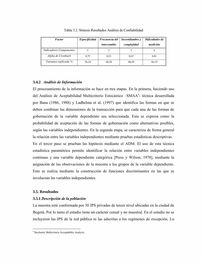
Tabla 3.2. Síntesis Resultados Análisis de Confiabilidad
3.4.2 Análisis de Información
El procesamiento de la información se hace en tres etapas. En la primera, haciendo uso
del Análisis de Aceptabilidad Multicriterio Estocástico –SMAA9- técnica desarrollada
por Bana (1986, 1988) y Ladhelma et al. (1997) que identifica las formas en que se
deben combinar las dimensiones de la transacción para que cada una de las formas de
gobernación de la variable dependiente sea seleccionada. Esta se expresa como la
probabilidad de aceptación de las formas de gobernación como alternativas posibles,
según las variables independientes. En la segunda etapa, se caracteriza de forma general
la relación entre las variables independientes mediante pruebas estadísticas descriptivas.
En el tercer paso se prueban las hipótesis mediante el ADM. El uso de esta técnica
estadística paramétrica permite identificar la relación entre variables independientes
continuas y una variable dependiente categórica [Press y Wilson, 1978], mediante la
asignación de las observaciones de la muestra a los grupos de la variable dependiente.
Esto se realiza mediante la construcción de funciones discriminantes en las que se
involucran las variables independientes.
3.5. Resultados
3.5.1 Descripción de la población
La muestra está conformada por 30 IPS privadas de tercer nivel ubicadas en la ciudad de
Bogotá. Por lo tanto el estudio tiene un carácter censal y no muestral. En el estudio no se
incluyeron las IPS de la red pública ni las adscritas a los regímenes de excepción. Lo
9 Stochastic Multicriteria Acceptability Analysis.
Factor Especificidad Frecuencia del
intercambio
Incertidumbre y
complejidad
Dificultades de
medición
Indicadores Componentes 5 2 3 4
Alpha de Cronbach 0,79 0,53 0,65 0,81
Varianza explicada % 56,14 68,54 60,44 66,19

anterior no implica que los resultados del estudio puedan extrapolarse a toda la
población. Esto porque no se indagó por todas las transacciones que realizaron las IPS
de la muestra con todas las EPS con las que tienen algún tipo transacción, sino que se
indagó por la transacción con una EPS.
Más del 70% prestan sus servicios hace más de 20 años y la totalidad de ellas realizan
procedimientos de alta complejidad. Son centros de referencia nacional para el manejo
de pacientes que se complican a pesar del tratamiento que se les ha dado en otras
instituciones.
Sólo dos de ellas hacen parte de complejos empresariales, y son las clínicas de
Colsubsidio y Saludcoop, mientras que las otras surgieron de manera independiente
aunque muchas tienen alianzas con aseguradoras. La Fundación Cardioinfantil y la
Clínica de la Fundación Abood Shaio se han subespecializado en el manejo de
patologías cardiovasculares, aunque prestan servicios de todas las especialidades
características del nivel. La Clínica del Niño y el Hospital la Misericordia se
caracterizan por atender a la población pediátrica. El Hospital San Ignacio y la Clínica
El Bosque, son universitarios.
Inicialmente, la forma de gobernación de intercambio de servicios de salud contemplaba
cuatro categorías, las cuales se redujeron a dos en el análisis empírico. La razón que
explica este hecho es que en el trabajo empírico la gobernación del intercambio de
servicios de consulta externa se dio mediante pago por servicio y capitación.
3.5.2 Análisis de las características de la decisión con SMAA
A partir de las distribuciones de las respuestas de cada uno de los indicadores de las
variables, se identificó, según las hipótesis, la forma de contratación que genera menores
costos de transacción para cada forma de intercambio. En la tabla 3 se presentan las
distribuciones de las respuestas asociadas a cada indicador utilizado en el análisis.

Los resultados muestran calificaciones relativamente bajas de los indicadores de la
variable de especificidad de las inversiones, lo que se permite pensar que la forma de
gobernación más eficiente es pago por servicio. Los indicadores de la variable
frecuencia del intercambio presentan valores relativamente altos, éste comportamiento
sugiere que la capitación puede ser la forma más eficiente de intercambio. Los
indicadores de incertidumbre en la prestación de los servicios y dificultades de
medición, presentan bajas calificaciones lo que según la teoría de costos de transacción
sugiere que la forma de gobernación a seleccionar sería el pago por servicio.
Tabla 3.3. Distribuciones de Probabilidad –Datos porcentuales-
Dados los anteriores resultados, el tipo de contratación que minimiza los costos de
transacción en la prestación de servicios de consulta externa no es fácilmente
determinable, ya que las variables no muestran una clara línea de decisión sobre la
manera como debe establecerse el intercambio.
Escala Likert de RespuestaVariables
1 2 3 4 5
Esp. 1. Dificultades reutilización inversiones físicas 23,3% 50% 20% 6,7% 0%
Esp. 2. IPS competidoras 20% 46,7% 33,3% 0% 0%
Esp. 3. IPS que podrían desarrollar servicios 23,3% 40% 20% 16,7% 0%
Esp. 4. Pérdida de rentabilidad si cambia de uso 30% 46,7% 20% 3,3% 0%
Esp. 5. Necesidad adaptar servicios 16,7% 16,7% 43,3% 23,3% 0%
Frec. 1. Frecuencia de intercambio 0% 6,7% 6,7% 43,3% 43,3%
Frec. 2. Estabilidad de los contratos 0% 6,7% 36,7% 30% 26,7%
Incert. 1. Dificultades seguimiento de protocolos 73,3% 20% 3,3% 3,3% 0%
Incert. 2. Complicaciones manejo de pacientes 76,7% 20% 0% 3,3% 0%
Incert 3. Dificultades para terminar tratamientos 43,3% 50% 3,3% 3,3% 0%
Dific. 1. Dificultad de medir resultados el paciente 70% 23,3% 6,7% 0% 0%
Dific. 2. Dificultad de medir EPS los resultados 80% 13,3% 3,3% 3,3% 0%
Dific. 3. Dificultad de medir calidad el paciente 80% 16,7% 3,3% 0% 0%
Dific. 4. Dificultad de medir calidad la EPS 70% 23,3% 3,3% 3,3% 0%

Para poder intentar dar solución al problema se puede hacer uso de técnicas que
permiten indagar más a fondo sobre la decisión. El SMAA surge como una herramienta
de decisión adecuada. La técnica indica el aporte de cada criterio a la minimización de
los costos de transacción, expresada en el término utilidad, en cada una de las formas de
gobernación posibles para el intercambio económico. Esto se hace operativo a través de
una adecuada función de utilidad aditiva como la que se presenta a continuación:
j
ijji uwu (3.1)
donde: ui = Utilidad total de la alternativa i; uij = Utilidad del criterio j para la alternativa
i; wj = Peso del criterio j.
El análisis proporciona estimaciones de los pesos de las variables -wj-, que permiten
calcular la utilidad de cada una de las posibles opciones de decisión. La técnica
determina los rangos de las combinaciones de las ponderaciones que hacen a cada una
de las formas de gobernación dominante sobre las demás en términos de utilidad.
También calcula el volumen del conjunto de las combinaciones de pesos de las variables
que hacen dominante a cada alternativa a las que se ha denominado, índices de
aceptabilidad. Finalmente determina los vectores de ponderaciones típicos –promedio-
de cada una de las opciones, como un centroide de cada uno de los hiperespacios que
soportan el dominio de una alternativa. –ver el Anexo B para una descripción detallada
de la metodología de análisis SMAA determinística-.
La utilidad, en este caso normalizada, de cada criterio por alternativa, fue calculada
como el promedio de las percepciones de cada una de las observaciones en las dos
categorías de la variable dependiente. Las utilidades típicas se presentan en la Tabla 3.4.
La variable que presenta una mayor diferencia en su valoración en las dos formas de
gobernación es la frecuencia del intercambio, por lo tanto se esperaría de esta variable
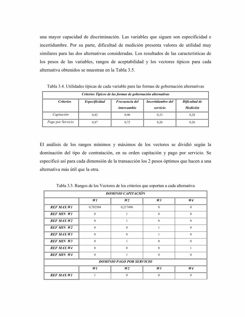
una mayor capacidad de discriminación. Las variables que siguen son especificidad e
incertidumbre. Por su parte, dificultad de medición presenta valores de utilidad muy
similares para las dos alternativas consideradas. Los resultados de las características de
los pesos de las variables, rangos de aceptabilidad y los vectores típicos para cada
alternativa obtenidos se muestran en la Tabla 3.5.
Tabla 3.4. Utilidades típicas de cada variable para las formas de gobernación alternativas
Criterios Típicos de las formas de gobernación alternativas
Criterios Especificidad Frecuencia del
intercambio
Incertidumbre del
servicio
Dificultad de
Medición
Capitación 0,42 0,90 0,33 0,28
Pago por Servicio 0,47 0,72 0,26 0,26
El análisis de los rangos mínimos y máximos de los vectores se dividió según la
dominación del tipo de contratación, en su orden capitación y pago por servicio. Se
especificó así para cada dimensión de la transacción los 2 pesos óptimos que hacen a una
alternativa más útil que la otra.
Tabla 3.5. Rangos de los Vectores de los criterios que soportan a cada alternativa
DOMINIO CAPITACIÓN
W1 W2 W3 W4
REF MAX W1 0,782504 0,217496 0 0
REF MIN W1 0 1 0 0
REF MAX W2 0 1 0 0
REF MIN W2 0 0 1 0
REF MAX W3 0 0 1 0
REF MIN W3 0 1 0 0
REF MAX W4 0 0 0 1
REF MIN W4 0 1 0 0
DOMINIO PAGO POR SERVICIO
W1 W2 W3 W4
REF MAX W1 1 0 0 0

REF MIN W1 0,300194 0 0 0,699806
REF MAX W2 0,782504 0,217496 0 0
REF MIN W2 1 0 0 0
REF MAX W3 0,585838 0 0,414162 0
REF MIN W3 1 0 0 0
REF MAX W4 0,300194 0 0 0,699806
REF MIN W4 1 0 0 0
VECTOR PONDERADO CENTRAL
W1c 0,20995005 0,26339754 0,26847778 0,25817462
W2c 0,66231843 0,05331346 0,10478811 0,17975886
Notación: Capitación, i = 1; Pago por servicio, i = 2; Especificidad, j=1; Frecuencia y Duración del intercambio, j=2; Incertidumbre
y Complejidad del servicio, j=3; Dificultad de Medición de la actuación, j=4.
El vector ponderado central que señala como forma de gobernación más adecuada a la
capitación -W1c- está dado por valores relativamente bajos en todas las dimensiones de la
transacción. Por otra parte, el vector ponderado central que muestra como forma de
gobernación más adecuada al pago por servicio –W2c- está dado por valores
relativamente altos de la especificidad -0,66-, valores bastante bajos de incertidumbre -
0,10- y dificultades de medición -0-17- y valores muy bajos para la frecuencia de la
transacción. En general los resultados son consistentes con las hipótesis; exceptuando el
signo de la especificidad de las inversiones, que muestra un sentido contrario. Valores
más altos cuando la forma de gobernación es el pago por servicio -0,66- que cuando se
opta por la capitación -0,20-.
Los mínimos y los máximos de cada una de las dimensiones que hace preferible
capitación o pago por servicios muestran, en general, que los rangos de dominancia son
bastante amplios. Para la incertidumbre se discuten los resultados continuación. El
vector factible que hace dominante a la capitación sobre el pago por servicio mediante la
maximización de la especificidad es: Especificidad = 0,78, Frecuencia del intercambio =
0,21, Incertidumbre del servicio = 0, Dificultad de Medición de medición = 0. Mientras
que el vector factible que hace dominante a la capitación sobre el pago por servicio
mediante la minimización de la especificidad es: Especificidad = 0, Frecuencia y

Duración del intercambio = 1, Incertidumbre y Complejidad del servicio = 0, Dificultad
de Medición de la actuación = 0.
Por otra parte el límite del rango posible que hace que el tipo de contratación de pago
por servicio sea dominante y que maximiza la ponderación de especificidad es 1, con las
demás ponderaciones de los criterios iguales a cero. A su vez el rango factible que
minimiza el valor de la ponderación del criterio de especificidad hace que éste tome un
valor de 0,3 y la dificultad de medición de la actuación tome 0,699 en la ponderación
con las demás variables ponderadas al 0. Análisis similares se realizan para los demás
criterios.
Tabla 3.6. Índices de Aceptabilidad
Finalmente, en la Tabla 3.6 se presentan los índices de aceptabilidad para cada
alternativa. Éstos muestran que aproximadamente el 93% de las combinaciones factibles
de las ponderaciones de los criterios responden a favor de la contratación de capitación.
Esto implica que la capitación debiese ser la forma de gobernación fundamental
mediante la cual se intercambiasen los servicios de consulta externa.
De lo anterior se puede concluir que la importancia de las variables en la selección de las
formas de contratación de los servicios de consulta externa cambia en función de la
forma de contratación. Si la frecuencia del intercambio es muy alta, es claro que el pago
por servicio es la forma más importante y la decisión se tomará en términos de costos de
operación, no obstante si la frecuencia es baja implica que el servicio se debe realizar
mediante capitación en tanto la especificidad sea alta, debido a la poca importancia de la
frecuencia en ésta forma de gobernación. Para frecuencias moderadamente bajas se debe
evaluar la especificidad, la incertidumbre y las dificultades de medición, variables que
tienen alta importancia en la capitación. Esto quiere decir que si el servicio es poco
Índices de Aceptabilidad (ai)
Capitación 0,930
Pago por servicio 0,070

específico y moderadamente bajas la incertidumbre y dificultades de medición son bajas
se deberá realizar el intercambio mediante pago por servicio, por el contrario si las
frecuencias son altas se debe contratar por capitación.
Como conclusión, dadas las condiciones de consulta externa lo más recomendable en
general es usar capitación, como se muestra en la Tabla 3.6.
3.5.3 Análisis del error de contratación: Pruebas estadísticas preliminares
Para el cumplimiento de las hipótesis estadísticas del ADM se deben satisfacer las
siguientes condiciones:
Normalidad de las variables independientes: la prueba estadística utilizada es la de
Kolmogorov-Smirnov. La hipótesis nula de normalidad de la variable es rechazada
cuando la significancia es inferior a 0,05, lo que implica un 95% de confianza del test.
Correlación entre las variables explicativas: las pruebas estadísticas utilizadas
corresponden a los coeficientes de correlación lineal de Pearson y Taub-Kendall, cuya
Hipótesis nula es la de no correlación entre las variables, la cual es rechazada cuando la
significancia es inferior a 0,05.
El grupo con menor cantidad de observaciones debe ser mayor al número de variables, la
distribución de observaciones entre los grupos debe ser similar y debe haber
homogeneidad de varianzas en las categorías o grupos de la variable dependiente, el
estadístico utilizado es el de Levene el cual se rechaza a un nivel se significancia de
0,05, ante la hipótesis nula de igualdad en la homogeneidad de varianzas en los grupos
de la variable. El último supuesto, siendo ésta la prueba más relevante, es el de igualdad
de las matrices de covarianzas, el estadístico utilizado es el M de Box el cual se rechaza
cuando la significancia es inferior a 0,05 ante hipótesis nula de igualdad entre las
matrices de varianzas-covarianzas de los grupos. Los resultados de éstas pruebas se
presentan a continuación.

Análisis de normalidad de las variables explicativas
La prueba de normalidad fue aplicada a los cuatro factores, sólo se rechazó la hipótesis
nula de ajuste de los datos a una normal en la variable dificultades de medición, con un
alpha de 0,009. Los resultados se presentan en la Tabla 3.7.
Tabla 3.7. Normalidad de los Factores
Variables Especificidad Frecuencia del
intercambio
Incertidumbre Dificultad de
Medición
Significancia 0,856 0,518 0,157 0,009
Análisis de correlación entre las variables explicativas: Se utilizó el coeficiente de
correlación de Pearson y Taúb-Kendall. Los resultados se presentan en la Tabla 3.8. Se
encontró que en general hay baja correlación entre las variables del modelo. La
correlación más alta se encuentra entre frecuencia y especificidad de las inversiones, lo
que se pudo también analizar en el SMAA.
Tabla 3.8. Prueba de Correlación entre los Factores
Variables Especificidad Frecuencia Incertidumbre Dificultades
Especificidad - -0,296 (0,030) 0,041 (0,769) -0,115 (0,416)
Frecuencia - - 0,091 (0,526) -0,015 (0,920)
Incertidumbre - - - 0,248 (0,099)
Dificultad - - - -
En paréntesis la significación estadística.
Análisis de homogeneidad de covarianza:
En la prueba de homogeneidad de varianza de Levene no se rechazó la hipótesis nula de
homogeneidad de varianza en ninguna de las variables. Los resultados se presentan en la
Tabla 3.9.
Tabla 3.9. Prueba de Homogeneidad de Varianza de las categorías de los Factores
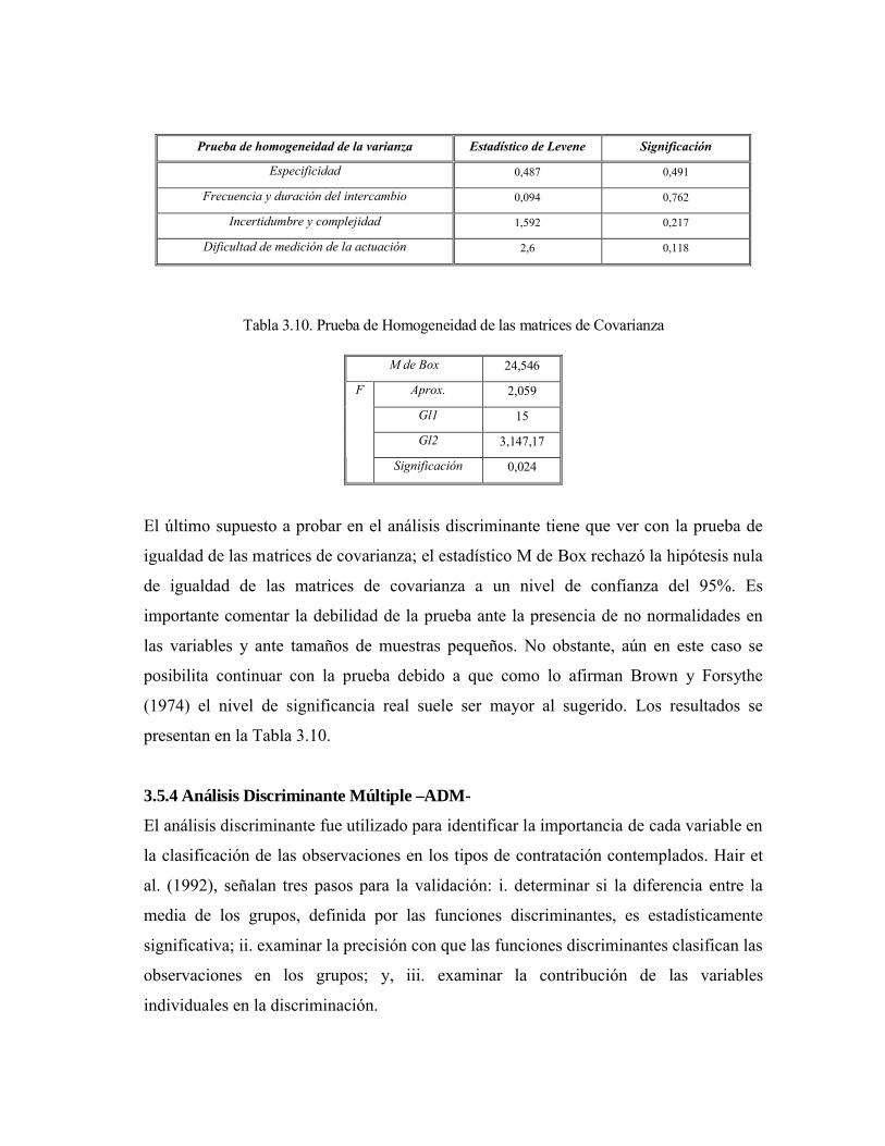
Tabla 3.10. Prueba de Homogeneidad de las matrices de Covarianza
El último supuesto a probar en el análisis discriminante tiene que ver con la prueba de
igualdad de las matrices de covarianza; el estadístico M de Box rechazó la hipótesis nula
de igualdad de las matrices de covarianza a un nivel de confianza del 95%. Es
importante comentar la debilidad de la prueba ante la presencia de no normalidades en
las variables y ante tamaños de muestras pequeños. No obstante, aún en este caso se
posibilita continuar con la prueba debido a que como lo afirman Brown y Forsythe
(1974) el nivel de significancia real suele ser mayor al sugerido. Los resultados se
presentan en la Tabla 3.10.
3.5.4 Análisis Discriminante Múltiple –ADM-
El análisis discriminante fue utilizado para identificar la importancia de cada variable en
la clasificación de las observaciones en los tipos de contratación contemplados. Hair et
al. (1992), señalan tres pasos para la validación: i. determinar si la diferencia entre la
media de los grupos, definida por las funciones discriminantes, es estadísticamente
significativa; ii. examinar la precisión con que las funciones discriminantes clasifican las
observaciones en los grupos; y, iii. examinar la contribución de las variables
individuales en la discriminación.
Prueba de homogeneidad de la varianza Estadístico de Levene Significación
Especificidad 0,487 0,491
Frecuencia y duración del intercambio 0,094 0,762
Incertidumbre y complejidad 1,592 0,217
Dificultad de medición de la actuación 2,6 0,118
M de Box 24,546
Aprox. 2,059
Gl1 15
Gl2 3,147,17
F
Significación 0,024

Tabla 3.11. Pruebas de igualdad de las medias de los grupos
El ADM evalúa la importancia relativa de las variables y la significancia estadística de
la distancia entre la media de los grupos: la significancia de la diferencia entre la media
de los grupos está dada por la prueba F de igualdad de las medias de los grupos, la
hipótesis nula de la prueba establece la igualdad de la media de los grupos. En el paso
siguiente, se analiza la contribución relativa de cada variable a la discriminación global
del modelo, y posteriormente, se estudia la participación de las variables significativas
en la diferenciación entre las dos categorías de contratación de la prestación de los
servicios de consulta externa. Los resultados se ilustran en la Tabla 3.11.
Las variables que son estadísticamente significativas son: frecuencia del intercambio e
incertidumbre, esto significa que la participación en la discriminación de las demás
variables debe ser cuidadosamente analizado.
La contribución relativa de cada variable en el modelo se define a partir de los
coeficientes discriminantes de las funciones incorporadas, los cuales se pueden ver en la
Tabla 3.12. El primer resultado relevante es la identificación de las variables no
significativas. Valores grandes de los coeficientes estandarizados presumen la
importancia de la variable en la discriminación, sin embargo la importancia real de la
variable solo puede estar justificada por el principio de parsimonia.
Pruebas de igualdad de las medias de los grupos F gl1 Gl2 Sig.
Especificidad de los servicios de salud 0,878 1 28 0,357
Frecuencia y duración del intercambio de servicios de salud 15,908 1 28 0,000
Incertidumbre y complejidad consulta externa 3,695 1 28 0,065
Dificultad de medición de la actuación consulta externa 0,474 1 28 0,497

Tabla 3.12. Coeficientes estandarizados de las funciones discriminantes canónicas
Se presentan ponderaciones relativamente altas en la mayoría de las variables en la
función discriminante, con la excepción de especificidad de las inversiones. Para
profundizar en el análisis se estudia la matriz de estructura; esta matriz permite
determinar el grado de correlación dentro de los grupos, entre las variables explicativas
y la variable de estudio. Altos valores de los coeficientes suponen altas correlaciones de
la variable con la función discriminante. Los resultados de la matriz de estructura se
presentan en la Tabla 3.13.
Los análisis permiten confirmar la importancia de la variable de frecuencia del
intercambio de servicios de salud y la poca importancia de la variable de especificidad y
dificultades de medición. Estas dos últimas variables relacionadas con los costos de
transacción no tienen capacidad de discriminación y por lo tanto no deben ser tenidas en
cuenta.
Tabla 3.13. Coeficientes de Correlación de los Factores con la Función discriminante
Matriz de estructura
Función
Frecuencia y duración 0,825
Incertidumbre y complejidad consulta externa 0,398
Especificidad de los servicios -0,194
Dificultad de medición de la actuación 0,142
Coeficientes estandarizados de las funciones discriminantes canónicas Función
Especificidad de los servicios -0,05
Frecuencia y duración del intercambio de servicios 0,921
Incertidumbre 0,536
Dificultad de medición de la actuación 0,121

Análisis posteriores se hacen necesarios para establecer la robustez de la función
discriminante; la cual se da cuando se tienen autovalores altos, alta correlación canónica
y valores pequeños del Lambda de Wilks; este último tiene asociado una prueba chi
cuadrado a la hipótesis nula de no diferencia entre las medias de los grupos, la prueba es
rechazada para valores de significancia inferiores a 0,1. Los resultados se presentan en la
Tabla 3.14.
Tabla 3.14. Pruebas de Validación de la Función Discriminante
De esta información se concluye que la función discriminante es estadísticamente
significativa. La correlación canónica indica que el 60,2% de la varianza de la variable
dependiente es explicada por las variables frecuencia del intercambio y la variable
incertidumbre. La prueba chi cuadrado rechazó la igualdad de las medias de los
centroides de las dos formas de contratación de la prestación de los servicios de consulta
externa a cualquier nivel de confianza.
Valoración de la precisión clasificatoria de las funciones discriminantes. El análisis
discriminante permite determinar las observaciones del servicio de consulta externa que
se clasifican de forma correcta. En 26 de los 30 casos se encontró una clasificación
correcta de las observaciones, esto es un 86,2%. Para que la precisión clasificatoria sea
aceptable debe ser un 25% mayor a la probabilidad proporcional [Hair et al. 1992], que
para el caso es: 50% * 1,25 = 62,5%, por lo tanto el modelo tiene una adecuada
capacidad de clasificar correctamente las observaciones de la población. La tabla 3.15
muestra la clasificación.
Autovalor 0,568
Correlación canónica 0,602
Lambda de Wilks 0,638 (0,000)

Tabla 3.15. Tabla de Clasificación
El porcentaje de observaciones correctamente clasificadas -hit ratio- por las funciones
discriminantes es del 86,7%, siendo bien clasificados el 84,6% de los casos de
capitación y 88,2% de pago por servicio. Es importante resaltar la importancia de cada
una de las dos variables consideradas por los tomadores de las decisiones; en este caso la
discriminación es debida en un 76,7% a la variable de frecuencia del intercambio de
servicios de salud, mientras que el restante 10% se le abona a la variable de
incertidumbre en la prestación de los servicios, la cual aporta únicamente a la buena
especificación de los casos de capitación.
3.6. Discusión de Resultados
El análisis discriminante múltiple muestra que las variables significativas en el modelo
son la frecuencia del intercambio e incertidumbre en la transacción. Esto quiere decir
que en la definición de la forma de gobernación de los servicios de consulta externa
responde fundamentalmente a la reducción de costos de producción mediante el logro de
economías de escala en la prestación del servicio de consulta externa. De forma
adicional, la incertidumbre en los resultados de la consulta externa afecta la forma de
gobernación de este tipo de servicios por parte de las EPS, y apoya a la toma de
decisiones a favor de la capitación cuando se considera alta.
Las aseguradoras contratan la prestación de servicios de consulta externa con las IPS
teniendo en cuenta el número de pacientes que remiten a cada institución. Cuando el
número de pacientes es bajo se contrata por servicios y cuando el número es alto se hace
Resultados de la
clasificación Forma de Contratación Grupo de pertenencia pronosticado Total
Capitación Pago por servicio
Capitación 11 2 13Recuento
Pago por servicios 2 15 17
Contratación 84,6 15,4 100%%
Pago por servicio 11,8 88,2 100%

mediante capitación. En estas circunstancias las IPS se ven forzadas a la reorganización
de los servicios de consulta externa tratando de estandarizar procesos para permitir el
logro de economías de escala y por lo tanto reducir los costos de prestación de los
servicios de salud.
Otro resultado agregado relevante es que solo la incertidumbre en la transacción, como
factor generador de costos de transacción, fue relevante en el modelo empírico. Esto
significa que en la prestación de servicios de consulta externa, la decisión sobre la forma
organizacional del intercambio está poco afectada por la existencia de costos de
transacción. Sin duda existirán costos de transacción y serán diferentes en las dos formas
de gobernación tenidas en cuenta en este estudio, pero no son tomados en cuenta en la
decisión que se está analizando. La implicación de este hallazgo es que posiblemente en
el intercambio de servicios de consulta externa se estén dando ineficiencias
transaccionales por la preponderancia que se le da a los costos de operación en la
prestación del servicio. Sobre este mismo aspecto, también cabe la posibilidad de que
sea un cargo administrativo muy alto el de tipificar la consulta externa para imputar su
costo a una determinada forma de contratación, no obstante a que los análisis favorezcan
a la contratación por capitación.
Por otra parte, la especificidad de las inversiones, además de no ser estadísticamente
significativo en la discriminación de las formas de gobernación muestra que el signo es
contrario al planteado en la hipótesis. Esto puede estar mostrando que en la toma de
decisiones sobre las formas de gobernación son poco importantes los factores asociados
a los costos de transacción. Teniendo en cuenta éstos hallazgos se considera relevante
profundizar sobre las variables transaccionales entre EPS e IPS en la prestación de
servicios de consulta externa10.
10 Una consideración que posiblemente deba hacerse es diferenciar entre las actividades médicas y administrativas. Si se hace referencia a la variable especificidad, altos valores se encontrarán en los procesos administrativos y no médicos. Estos últimos podrían darse cuando alguna EPS tenga una población con ciertas características que impliquen de forma preferencial cierto tipo de tratamiento o de dolencias, como podría ser con la atención de pilotos de aviación.

Por último, posiblemente el establecimiento de mecanismos de comunicación y control
característicos de las jerarquías en las prestación de servicios de consulta externa
mediante formas capitadas se hace con el fin de soportar la prestación del servicio de
salud y disponer de información que permita planear y ajustar actividades futuras, no
para ejercer control de costos y del tipo de servicios que se prestan en cada una de las
intervenciones. Esto porque la EPS, cuando compra de forma capitada lo que busca es
precisamente reducir sus costos de auditoría.
3.7. Referencias
Albaum, G. (1997), The likert scale revisited: an alternative version. Journal of the
Marketing Research Society 19(2) 331-348.
Alchian, A., Woodward, S. (1988), The firm is dead; long live the firm. A review of
Oliver E. Williamson´s: The economic institutions of capitalism”, Journal of
Economic Literature 26 65-69.
Álvarez, B. Pellisé, L., Lobo, F. (2000), Sistemas de Pago a Prestadores de Servicios de
Salud en Países de América Latina y de la OCDE. Revista Panamericana de Salud
Pública 8 55-70.
Arrow, K. J. 1962. Economic Welfare and the Allocation of Resources for Invention,
versión en castellano, Rosenberg, N. Economía del cambio tecnológico, México,
Fondo de Cultura Económica, 1979.
Bana, C. (1986), A Multi-criteria Decision Aid Methodology to Deal With Conflicting
Situations on the Weights. European Journal of Operational Research 26 22-34.
____ (1988), A Methodology for Sensitivity Analysis in Three Criteria Problems: A case
study in municipal management. European Journal of Operational Research, 33:
159-173.
Barzel, Y. 1989. Economic Analysis of Property Rights, Cambridge uk, Cambridge
University Press.
Brown, M.B., Forsythe, A.B. (1974), Robust Tests for the Equality of Variances
Journal of the American Statistical Association, 69: 364-367.

Chi, T. 1994, Trading in Strategic Resources: Necessary Condition, Transaction Costs
Problems And Choice Of Exchange Structure. Strategic Management Journal 15
(4) 271-290.
Churchill, G.A. (1979), A paradigm for developing better values of marketing
constructs. Journal of Marketing Research 16 64-74.
Coase, R. H. (1937), The nature of the firm. Economica, November: 386-405.
Doty, D. H., Glick, W. H. (1994), Typologies as a Unique Form of Theory Building:
Toward Improved Understanding and Modeling. Academy of Management
Review 19 230-251.
Enthoven, A. C. 1997, The Market-based Reform of America`s Health Care Financing
and Delivery System: Managed Care and Managed Competition. A Conference
Sponsored by the World Bank March 10-11.
Erramilli, M.K., Rao, C. P. (1990), Choice of Foreign Market Entry Modes for Service
Firms: Role of Market Knowledge. Management of International Review 30 135-
150.
Gorbaneff, Y., Torres, S., Contreras, N. (2004), Anatomía de la Cadena de Prestación de
Salud en Colombia en el Régimen Contributivo. Cuadernos de Administración
3(6) 88-106.
Gutiérrez, C., Molina, C. G., Wüllner, A. (1995), Las Formas de Contratación entre
Prestadoras y Administradoras de Salud, Fedesarrollo, Bogotá.
Hair, J. F., Anderson, R. E., Tatham, R. L., Black, W. C. (1992), Multivariate Data
Analysis, Prentice Hall, 4a Edición, New Jersey.
Hart, O. (1991), Incomplete Contracts and the Theory of the Firm. Williamson, Oliver,
The Nature of the Firm, Oxford University Press, New York Oxford. 138-158.
Hage, J., Alter, C. (1997), A typology of interorganizational relationships and networks.
Contemporary Capitalism: The embeddedness of institutions, J. R. Hollingsworth
R. Boyer (Eds.), Cambridge University Press. 94-126.
Johnson, R., Wichern, D. (1999), Applied multivariate statistical analysis, Fourth
Edition, Prentice Hall.
Johnson, R., Wichern, D. (1987), The Detection of Influential Observations for
Allocation, Separation, and the Determination of Probabilities in a Bayesian
Framework. Journal of Business and Economic Statistics 5(3) 369-381.
Kim, W. C. Hwang, P. (1992), Global Strategy and Multinationals Entry Mode Choice.
Journal of International Business Studies 23: 29-53.
Kerlinger, F. N. (1986), Foundations of Behavioral Research, Harcout Brace College
Publishers, 4a Edición, Fort Worth.
Lahdelma, R., Hokkanen, J., Salminen, P. (1997), SMAA–Stochastic multiobjetive
acceptability analysis. European journal of operational research,106 137-143.
Lewin, A. Y., Volverda, H. W. (1999), Prolegomena on coevolution: A framework for
research on strategy and new organizational forms. Organization Science 10(5)
519-534.
Li, P. (1998), Toward a Geocentric Framework of Organizational Form: A Holistic,
Dynamic and Paradoxical Approach. Organization Studies 19 829-861.
Londoño, J. L., Frenk, J. (1997), Pluralismo Estructrurado: Hacia un Modelo Innovador
para la Reforma de los Sistemas de Salud en América Latina, Banco
Interamericano de Desarrollo. Documentos de Trabajo No. 353.
Lothia, R., Brooks, C. M., Krapfel, R. E. (1994), What constitutes a transaction specific
asset?. Journal of Business Research 30 261-270.
Malagón, G. y Otros (1986), Administración Hospitalaria, Editorial Médica
Panamericana, Bogotá, Colombia.
Mang, P. Y. (1994), The economic organization of innovation by R&D-Intensive firms:
An empirical analysis of the biopharmaceutical industry, Doctoral Dissertation,
Harvard University, Boston.
Milgrom, P., Roberts, J. (1993), Economía, organización y gestión de la empresa, Ariel
Economía, Barcelona.
Molina, C. (1995), Las Formas de Contratación entre Prestadoras y Administradoras de
Salud en el Nuevo Marco de Seguridad Social, Fundación Social, Bogotá.
Nunnally, J. C. (1978), Psycometric Theory, McGraw Hill, New York.

Pisano, G. P. (1988), Innovation through markets, hierarchies, and joint ventures:
Technology strategy and collaborative arrangements in the biotechnology industry,
Doctoral dissertation, University of California, Berkeley.
Porter, M., Fuller, M. B. (1986), Coalitions and global strategy. In Competition in global
industries, Michael Porter (Ed.), 315-343.
Press, J., Wilson, S. (1978), Chosing Between Logit and Discriminant Analysis. Journal
of Economic Literature 73 699-705.
Rencher, A. C. (1992), Interpretation of Canonical Discriminant Functions, Canonical
Variates and Principal Components. The American Statistician 46 217-225.
Seshadri, S. (2005) Sourcing strategy. Estados Unidos. Springer
Teece, D. J. 1986. Profiting from Technological Innovation: Implications for Integration,
Collaboration, Licensing and Public Policy. Research Policy 15 285-305.
Torres, S. (2003), Firm boundaries in the technological innovation chain: the machine-
tool industry in the Basque Country. Management Research 2(1) 49-65.
____, Gorbaneff, Y., Contreras, N. (2004), Caracterización de las formas de gobernación
del intercambio económico. Cuadernos de Administración 17(27) 63-86.
Steuer, R., (1986), Multiple Criteria Optimization: Theory, Computation, and
applications, John Wiley and sons, New York.
Williamson, O. E. (1975), Markets and hierarchies, analysis and antitrusth implications,
Free Press, New York.
____ (1985), The Economic institutions of capitalism, Free Press, New York.
____ (1991), Comparative economic organization: The analysis of discrete structural
alternatives. Administrative Science Quarterly 36 269-296.

Apéndice B. Análisis de Aceptabilidad Multicriterio Estocástica –SMAA-
Notación:
Constantes:
m = Número de alternativas
n = Número de criterios
Índices:
i є {1, 2, ...m} índice para las alternativas.
j є {1, 2, ...m} índice para los criterios.
Otros símbolos:
gij = Valor del criterio j para la alternativa i
ui = Utilidad total de la alternativa i
uj(gij) = Función de utilidad del criterio j dentro del rango [0,1]
uij = Utilidad del criterio j para la alternativa i
w = Vector de pesos [w1….wn]
wj = Peso para el criterio j
wib = Peso básico favorable para la alternativa i
wic = Peso central del vector para la alternativa i
W = Conjunto de posibles vectores de peso
Wi = Conjunto de vectores de peso favorables para la alternativa i
Metodología:
La técnica se encuentra apoyada en el valor típico de cada criterio para cada alternativa
(gij). A partir de dichas decisiones se calculan las funciones de utilidad de cada criterio j
para cada alternativa i mapeándolas en el intervalo uniforme [0,1]. Se utilizará una
función de utilidad aditiva -la cual no es restrictiva-, de tal manera que la utilidad total
de la alternativa i será el resultado de la suma de los productos de las ponderaciones
convexas factibles de cada criterio por la función de utilidad de cada criterio de la
alternativa i. La descripción matemática se muestra a continuación:

10
)(
jj
jijj
ijjij
wwR*;wW
W, wuwiu
guu
(B.1)
Una alternativa será dominante cuando su función de utilidad supere a las funciones de
utilidad de las alternativas competidoras. Dado que el espacio factible W, es un politopo
convexo de dimensión (n-1), el problema de hallar una solución básica del conjunto de
pesos favorables para la alternativa i, puede ser resuelto a partir de una formulación de
programación lineal. Esta se representa a continuación:
0
1
11
0max
j
jj
j jkjjijj
w
w
,...,m;k, kuwuw
(B.2)
La solución del problema permite determinar si existe por lo menos un vector de pesos
que hagan a la alternativa i dominante. Por razones de la convexidad del politopo el
conjunto solución es una combinación convexa de sus vértices, lo cual se expresa a
continuación:
b
bbbi
bi wwRww 01: (B.3)

Los rangos de los pesos es un factor importante para la toma de la decisión, ya que los
pesos deben cumplir con algunas condiciones impuestas por la naturaleza del problema.
Los rangos pueden ser eficientemente obtenidos a partir de la siguiente formulación:
0
1
11
maxmin
j
jj
j jkjjijj
j
w
w
,...,m;k, kuwuw
)w(
(B.4)
Un resultado importante para la decisión final, es la determinación del índice de
aceptabilidad para cada alternativa, el cual se encuentra definido como la probabilidad
del volumen de los pesos de la alternativa en relación con el volumen de pesos factibles.
Valores cercanos a cero de una alternativa, indica un bajo volumen de combinaciones de
pesos factibles que hacen a la alternativa dominante. La representación matemática se
expresa a continuación:
Wvol
Wvola
dwWvol
ii
w
i
i
(B.5)
Finalmente podemos argumentar que sin conocimiento a priori de las decisiones de los
tomadores de la decisión, el vector de pesos central es la mejor representación de un
decisor típico. Se define como el centro de gravedad del volumen factible de los pesos
de la alternativa; como se expresa en la siguiente ecuación:

i
i
w
wci
dw
wdw
w (B.6)

CHAPTER FOUR
Send to European Journal of Operational Research
Status: Accepted

Integral Analysis Method – IAM
Rafael Guillermo García Cáceres*
Julián Arturo Aráoz Durand**
Fernando Palacios Gómez***
Abstract:
This paper presents the theoretical foundations of the new Integral Analysis Method
(IAM), and its application to a facility location problem. This methodology integrates
the cardinal and ordinal criteria of combinatorial stochastic optimization problems in
four stages: definition of the problem, cardinal analysis, ordinal analysis and integration
analysis. The method uses concepts of Stochastic Multicriteria Acceptability Analysis
(SMAA), Monte Carlo Simulation, Optimization Techniques and Elements of
Probability. The proposed method (IAM) was used to determine optimal locations for
the retail stores of a Colombian coffee marketing company.
Key Words: Multiple Criteria Analysis; Multiple Objective Programming,
Combinatorial Optimization; Simulation; Integral Analysis Method.
4.1. Introduction
Integral Analysis Methodology - IAM - is a decision-making technique that comes out
as a response to the technical difficulties that emerge in considering cardinal and ordinal
variables when they are both relevant to a stochastic optimization problem.
Just like previous techniques developed by the pioneer works of Bana e Costa,
Hokkanen, Lahdelma, Miettinen, Salminen, Makkonen and Tervonen (1998-2007),
Integral Analysis Methodology is used whenever it is impossible or inconvenient to
determine a priori the importance of each of the variables that support the decision.
This article is the result of a research project “Optimization of Agro-industrial Chains in Colombia” carried out by the Universidad de la Sabana and the Pontificia Universidad Javeriana with the financial support of COLCIENCIAS (Spanish acronym for Colombian Institute for the Development of Science and Technology ‘Francisco José de Caldas’) and the Universidad de la Sabana.Email: *[email protected], **[email protected], ***[email protected].
This new methodology for decision-making problem solving is a combination of
optimization techniques (i.e., mathematical programming, heuristics or simulation),
SMAA techniques, probability elements, and the development of new concepts framed
in the four phases proposed: definition of the problem, cardinal analysis, ordinal analysis
and integration analysis.
IAM is based on the technical processing of variables depending on their particular type
(ordinal or cardinal). It’s indicators are expressed in homogeneous units that can be
naturally integrated. The technique is particularly appropriate when the decision
environment is characterized by randomness, and deterministic simplifications are not
acceptable as possible solutions. In simpler contexts the problem can be solved by using
more traditional approaches like optimization or SMAA-type techniques.
4.2. Background
The decision-making process of multicriteria methods is based on the selection of a set
of alternatives by means of preference information provided by the decision-makers
[Keeney and Raiffa, 1976]; [Saaty, 1980]; [Steuer, 1986]; [Zeleny, 1990]; [Vincke,
1992].
However, in public decision making environments, problems may arise when those who
are responsible for the decision making process are unwilling or unable to openly
express their preferences. In order to solve this problem, Bana e Costa (1986, 1988),
introduced a procedure based on indicators that suggested the acceptance of a single
alternative when the decision is supported on three variables. Later on, and based upon
the above mentioned work, Lahdelma, Hokkanen, Salminen, Miettinen and Tervonen
(1998-2007)12 furtherly developed the methodology in various ways: they initially
generalized it into a multi-dimensional space [Lahdelma, et al., 1998], and then,
depending on the nature of each alternative's matrix of variable values, they presented
12 These methodologies are here referred to as Stochastic Multiobjective Acceptability Analysis (SMAA).

more sophisticated treatment mechanisms, such as different versions of SMAA for
imprecise data [Miettinen and Salminen, 1999] and stochastic data values [Lahdelma, et
al., 1998]. In turn, SMAA-O applies for mixed cardinal and ordinal data values
[Lahdelma, et al., 1999] and is currently capable of treating missing and imprecise
preference information as well [Lahdelma, et al., 2003]. Other works include Gaussian
criteria [Lahdelma, et al., 2006], cross confidence factors [Lahdelma and Salminen,
2006a], SMAA-D, which has been developed for Data Envelopment models [Lahdelma
and Salminen, 2006b] and SMAA implementation techniques [Tervonen and
Lahdelma, 2007]. Finally, cardinal and ordinal data can well be dealt with in the new
approach to multi criteria decision methods called Dominance-based Rough Set
Approach [Greco, et al., 2001, 2005], [Slowinski, et al., 2005].
One of the possible limitations of multiobjective decision-making techniques arises
when not all the ranking values are of the same kind. For example, if the prevailing type
is that of ordinal values, the cardinal variables must be expressed in ordinal terms.
On the other hand, in spite of the evident advantages of optimization techniques in
providing optimal solutions to different problems, they do not allow the inclusion of
relevant variables that cannot be expressed in terms of their objectives, and must then be
ignored. In such context, IAM was developed with the purpose of gathering and taking
advantage of the most relevant features of the mentioned techniques.
4.3. The Process of IAM
The two types of variables (ordinal and cardinal) inherent to many optimization
problems have a manifest operational complexity resulting from the metric and
epistemological difficulties that hinder their integration. This difficulty reduces the
possibility of finding well-designed solutions, and allows the use of more-relaxed
approximations. The conflict that arises when dealing with ordinal and cardinal variables
at the same time can be caused by:

The impossibility to express ordinal variables that are relevant to the ‘optimal’
solution of the problem, in cardinal terms (that is, regarding the objective goals). In
this case, such variables are not included and cannot be integrated in the
optimization technique that supports the decision.
The relaxation of cardinal variables as a result of transformations (for example, of
the ordinal type). In this case, important information contained in the variable is lost
and validity problems arise due to the categorization procedure.
Mathematical techniques such as simulation and optimization are commonly used when
the inclusion of the ordinal variables involved in the problem is considered irrelevant, or
when such variables cannot be taken into account due to either information or
implementation restrictions.
On the other hand, some multiobjective decision-making techniques fall into the second
type of inadequate specification, since they show difficulties in the treatment of
causality, and in the finding of suitable solutions to optimize the relevant objectives.
Due to the technical and practical impossibility that arises in homogenizing ordinal
aspects in cardinal terms, optimization techniques often resort to the relaxation of many
aspects that are relevant to the problem, therefore providing sub- optimal solutions.
IAM actually aims to overcome the obstacles that arise with some methodologies that do
not include all the relevant variables of a stochastic problem because they are not
adequately expressed in terms of their objective performance valuation. This
methodology provides the technical means that allow relevant ordinal variables to be
taken into account, therefore attaining closer to reality solutions.
This methodology comprises four steps: Definition of the Problem, Cardinal Analysis,
Ordinal Analysis, and Integration Analysis; which are now explained in more detail:

4.3.1. Definition of the Problem.
At this stage, both the type of problem (cardinal and/or ordinal) and its stochastic or
deterministic nature are established, and so are the objective(s), variables and
performance constraints for the selected models, together with their solving techniques.
Several reliable information collecting mechanisms are necessary to determine the
parameters, together with adequate procedures to estimate them, so that they correspond
to the models in use.
This is the most sensitive step of IAM in terms of consistency, due to methodological
difficulties and restrictions in the information sources. At this point, Delphi techniques
may help to create an atmosphere where agreements between the parties involved in the
project can take place.
4.3.2. Cardinal Analysis.
In a combinatorial problem, if the number of binary decision variables α is an
unrestricted and known quantity, it could entail up to 2α solving possibilities (also called
alternatives). Only then are the characteristics of the cardinal solution analyzed.
Sets and constants
F: Alternatives set
N(*): Number of states of the set *
m: Number of selected alternatives and cardinal rankings associated with them, where m ≤ 2α
Other Symbols
z(i): Cardinal ranking for alternative i
Φk: Binary variable, where Φk є {0, 1}
ei: Binary variable vector for alternative i, where ei = {Φ1, Φ2,… Φm}.
p(ei): Joint cardinal probability distribution for alternative i
p(Φk): Marginal cardinal probability distribution for variable k
hi : Random variable for alternative i
g(hi) : Probability density function for alternative i

Ei: Expected cardinal value for alternative i
2iσ : Variance cardinal value for alternative i
E: Overall central cardinal value
σ2: Overall dispersion cardinal value
In order to deal with the stochastic nature of the parameters employed in optimization
techniques, a Monte Carlo simulation is applied. The mathematical optimization model
is executed as many times as necessary until the results can be estimated with sufficient
precision. As a result of the Monte Carlo simulation, the joint cardinal probability
distribution is obtained.
The marginal cardinal probability distribution can be easily calculated from the joint
cardinal probability distribution, as follows:
(4.1)
The joint cardinal probability distribution mentioned above depends on the interaction
between the probability functions of the random variables of the problem’s parameters.
At this stage of the solution of the problem, a set F, constituted by the m selected
alternatives of interest to be analyzed by the DMs (which correspond to the number of
associated cardinal rankings), comes out as a result of the process. A possible selection
procedure consists in removing of the analysis those alternatives with very low
probability of occurrence. The prevailing alternatives will be studied later, in the ordinal
and integration analysis stages.
On the other hand, the cardinal ranking of each alternative will depend on its probability
of occurrence; the higher the latter, the lower the former.
k)(ep)P( im
ik
1
1

The objective function value associated to an alternative solution is a continuous
random variable hi with an associated density g(hi). The expected cardinal value and the
variance cardinal value of each of the selected alternatives are computed as follows:
(4.2)
Finally, and based upon the expected cardinal values of the alternatives, the overall
central value and the dispersion cardinal value are obtained.
(4.3)
4.3.3. Ordinal Analysis.
The ordinal analysis is based on Stochastic Multiobjective Acceptability Analysis with
ordinal data (SMAA-O) and is restricted to the m alternatives resulting from the cardinal
analysis. This phase is particularly complex because of the difficulties that usually arise
when defining the matrix of typical relative values that will be used as input for SMAA-
O. The utility of each alternative solution is a function of the particular utilities of all its
ordinal variables.
The SMAA-O method allows working with both ordinal and cardinal criteria. Although
widely used, this procedure has the following undesirable feature:
Risk of distorting the information contained in the cardinal variable as a result of the
transformation. When using this method, it is necessary to subordinate the number of
categories of each cardinal variable to the number of ordinal variables. In addition, a
idhhgEhE
idhhghE
iii
ii
iiii
)()(
)(
2
m
i
ii2
m
i
ii
epE(E
epEE
1
1
)()
)(
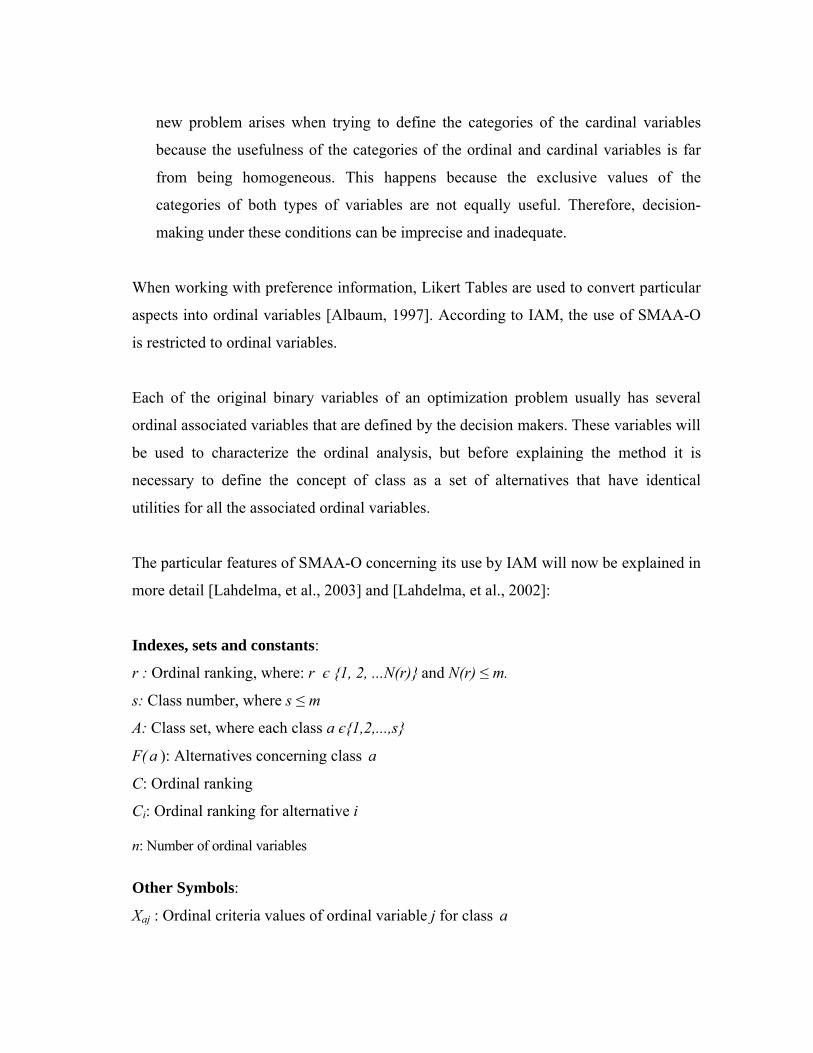
new problem arises when trying to define the categories of the cardinal variables
because the usefulness of the categories of the ordinal and cardinal variables is far
from being homogeneous. This happens because the exclusive values of the
categories of both types of variables are not equally useful. Therefore, decision-
making under these conditions can be imprecise and inadequate.
When working with preference information, Likert Tables are used to convert particular
aspects into ordinal variables [Albaum, 1997]. According to IAM, the use of SMAA-O
is restricted to ordinal variables.
Each of the original binary variables of an optimization problem usually has several
ordinal associated variables that are defined by the decision makers. These variables will
be used to characterize the ordinal analysis, but before explaining the method it is
necessary to define the concept of class as a set of alternatives that have identical
utilities for all the associated ordinal variables.
The particular features of SMAA-O concerning its use by IAM will now be explained in
more detail [Lahdelma, et al., 2003] and [Lahdelma, et al., 2002]:
Indexes, sets and constants:
r : Ordinal ranking, where: r є {1, 2, ...N(r)} and N(r) ≤ m.
s: Class number, where s ≤ m
A: Class set, where each class a є{1,2,...,s}
F( a ): Alternatives concerning class a
C: Ordinal ranking
Ci: Ordinal ranking for alternative i
n: Number of ordinal variables
Other Symbols:
Xaj : Ordinal criteria values of ordinal variable j for class a

wj : Weights vector of ordinal variable j
uj(Xaj) : Mapping of ordinal criteria values of variable j for class a
jr : Random number taken from a [0,1] uniform distribution
εaj : Stochastic cardinal values of criterion ordinal variable j in class a )
raW : Set of favourable weights in ordinal ranking r for class a:
W: Set of non-negative normalized weights
rab : Ordinal acceptability index for class a
rib : Ordinal acceptability index for alternative i
ci: Number of ordinal rankings of alternative i
R i : Ordinal ranking central value for alternative i
V i: Deviation value of the ordinal ranking for alternative i
The ordinal analysis is based on determining the utility values that support each class.
The utility function can be additive, as in the following case:
(4.4)
The process starts by generating random numbers out of a uniformly distributed [0, 1]
interval and sorting them along with 1 and 0 in decreasing order, as shown below:
(4.5)
Such procedure ranks these random numbers just as in previous works [Miettinen et.al.
1999; Lahdelma et al., 2002]. The distinctness of γjr can be ensured by rejecting sets
containing identical values. On the other hand jmax refers to the maximum number of
different rank categories of possible solutions for each of the selected variables.
1321001 max121 maxmax ,..,j,k),,U(γand,γ,γwhere:,γγγ jkjjjjj.......jj
)(Xuww),u(X ajj
n
1jja

These numbers are used as a sample of stochastic cardinal values of criterion ordinal
variable j in class a (εaj ), so that for each class a, the corresponding value is equal to
γjr; thus:
(4.6)
where the elements of ε є X are distributed according to f (ε): }εf{εX , being
(X) the set of stochastic cardinal utilities. All stochastic cardinal assignments must
comply with the following requirements in order to find the weight sets:
(4.7)
Thus, the accepted stochastic cardinal values and convex weights will be those that
conform to the ordinal ranking of the alternative. In order to make sure that each
alternative is assigned an adequate ranking, the (alternatives') utility functions are
compared by means of the following function:
(4.8)
Here each alternative is ranked from 1 to s. The ranking function’s objective is to obtain
the set of feasible variable weights associated to each ranking, by assigning cardinal
utilities. The process is mathematically represented as follows:
(4.9)
Finally, the ordinal acceptability index, which assesses the variation between different
values under ranking r in class a, is calculated through a multidimensional integral over
the criteria distributions and the favourable rank weights:
ajjraj Xr,γε
ajajj ε)(Xu
0111
ρ(false),ρ(true)where:,w),εw,ρ(ε,w)(ε a
s
kkarank
n
jj
n
ar
a
w,w:RwW
r,wεW:wεW
1
10
rank

(4.10)
Each of the alternatives' ordinal ranking can be easily obtained by assigning them to the
ordinal ranking that corresponds to the class to which they belong, so that
(4.11)
Decision making in this ordinal context consists in setting an agreement that is based on
the particular features of the feasible weights and the acceptability indexes; the latter
support the ordinal ranking of each alternative.
Thus, as a result of the cardinal modelling process, a set F of optimal possible solutions
for the combinatorial problem is obtained. This set is made up of m alternatives that
constitute the input of the ordinal analysis, as a result of which, a set of ordinal rankings
(Ci) associated to each alternative is also obtained.
(4.12)
The number of ordinal rankings for each alternative is lower or equal to m, because there
may be some alternatives with zero ordinal acceptability indexes for some ordinal
rankings. Finally, the number of ordinal rankings for the set (C) of alternatives is given
by:
(4.13)
For each alternative, the ordinal ranking central value and its associated (ordinal
ranking) deviation value are given by:
dεdwwfεfbX εw
ar
ra
F(a)ibb ar
ir
mc)N(Cwhere:,s,..,,C iii 21
2
1
:, mN(C)swherecN(C)m
ii

(4.14)
It is important to point out that these two values respectively correspond to the ordinal
ranking expected value and the ordinal ranking variance value, for the class to which the
alternative belongs.
4.3.4. Integration Analysis.
The cardinal and ordinal analyses help to determine a set of results that significantly
support the decision making process. At the same time, these results are the input of the
integration procedure that provides the indicators which are going to facilitate the
analysis of the problem in a broader context.
An important methodological consideration is the selection of the number of both types
of rankings. As it was previously mentioned, removing low probability alternatives may
be an appropriate procedure to limit the number of cardinal solutions. Moreover, the
class concept allows the grouping of the selected alternatives, thus reducing the
complexity of the ordinal analysis. On the other hand, the number of ordinal rankings
that were used in the integration stage may be restricted to the first ranking in most
practical cases. However, decision makers are the ultimate responsibles for the definition
of the problem size in its different analysis stages. The integration ranking of each
alternative is conditioned by the ordinal analysis ranking because each optimal cardinal
solution may have a different ordinal ranking status. The integration analysis is
presented as follows:
The joint integral index is defined as: pr(ei)
m
r
ir
2ii
m
r
ir
i
b)R-(rV
rbR
1
1
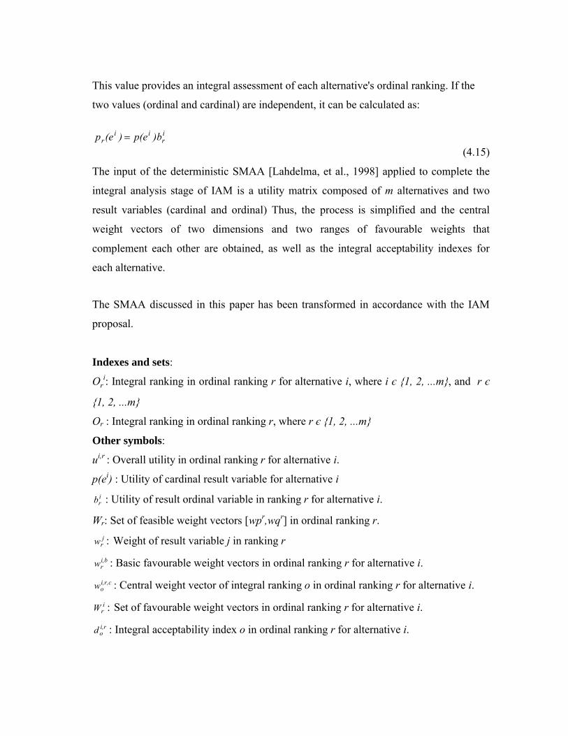
This value provides an integral assessment of each alternative's ordinal ranking. If the
two values (ordinal and cardinal) are independent, it can be calculated as:
(4.15)
The input of the deterministic SMAA [Lahdelma, et al., 1998] applied to complete the
integral analysis stage of IAM is a utility matrix composed of m alternatives and two
result variables (cardinal and ordinal) Thus, the process is simplified and the central
weight vectors of two dimensions and two ranges of favourable weights that
complement each other are obtained, as well as the integral acceptability indexes for
each alternative.
The SMAA discussed in this paper has been transformed in accordance with the IAM
proposal.
Indexes and sets:
Ori: Integral ranking in ordinal ranking r for alternative i, where i є {1, 2, ...m}, and r є
{1, 2, ...m}
Or : Integral ranking in ordinal ranking r, where r є {1, 2, ...m}
Other symbols:
ui,r : Overall utility in ordinal ranking r for alternative i.
p(ei) : Utility of cardinal result variable for alternative i
irb : Utility of result ordinal variable in ranking r for alternative i.
Wr: Set of feasible weight vectors [wpr,wqr] in ordinal ranking r.
jrw : Weight of result variable j in ranking r
i,brw : Basic favourable weight vectors in ordinal ranking r for alternative i.
i,r,cow : Central weight vector of integral ranking o in ordinal ranking r for alternative i.
irW : Set of favourable weight vectors in ordinal ranking r for alternative i.
i,rod : Integral acceptability index o in ordinal ranking r for alternative i.
ir
iir )bp(e)(ep
iro : Number of integral states in ordinal ranking r for alternative i.
pr(ei): Joint integral index in ordinal ranking r for alternative i.
The overall utility of each alternative is based on the typical relative values of its result
(that is, the utility of cardinal and ordinal result variables). An additive utility function
will be used, so that the overall utility of each alternative will be the result of adding the
products of the feasible convex weight of each variable and its associated utility. The
following is the mathematical description:
(4.16)
The set of favourable weight vectors Wr is a one-dimensional simplex in the bi-
dimensional weight space. An alternative is dominant when its utility surpasses those of
all other alternatives. The problem of finding a set of basic favourable weights for
integral ranking o is solved for each ordinal ranking r by means of the following LP:
(4.17)
The set of basic favourable weights wri is a convex polytope that can be represented as a
convex combination of its vertices:
(4.18)
The set of basic favourable weights for each result variable constitutes an important
element in the decision making process, since it must comply with the conditions
imposed by the nature of the problem. These sets can be efficiently obtained for each
ordinal ranking r from the solution of the following LP:
p,qjw
ww
ih,..m,,hbw)p(ewbw)p(ew
to:subject
Max
jr
qr
pr
hr
qr
hpr
ir
qr
ipr
0
1
21
0
b brr
i,brrrr
ir
bbb
α,α,wαw:Rww 01
102
qr
prrrr
ir
qr
ipr
ir
ww,w,RwW
RrW,, wbw)p(ewu

(4.19)
The integral acceptability indexes for each alternative in ordinal ranking r are defined as
the ratio between the alternative's weight volume and feasible weight volume, both in
that same ranking; which gives the alternative an integration ranking o. A low integral
acceptability value o (close to zero) for an alternative in any ordinal ranking r implies a
low number of favourable weight combinations, which makes this (alternative) the
dominant one. The following is the mathematical representation:
(4.20)
Finally, it can be stated that without any prior knowledge of the decision makers’
expertise, the central weight vector is the best representation of a typically non biased
decision maker. The central weight vector in ordinal ranking r for integral ranking o, is
defined as the center of gravity of the polytope:
(4.21)
The set of integral rankings in ordinal ranking r for each alternative i (Ori), is given by
the following states: Ori Є{1, 2,.., m}; which is made up of or
i states:
(4.22)
p,qjw
ww
ih,..m,,hbw)p(ewbw)p(ew
tosubject
w)(
jr
qr
pr
hr
qr
hpr
ir
qr
ipr
jr
0
1
21
maxmin
mo)N(O ir
ir
0
iri
r
i,roi,r
o
w
ri,r
o
WvolWvol
Wvold
dwWvolir
ir
ir
w
wci,ro
dw
wdw
w ,

Therefore, the integration set in a particular ranking Or is presented as the union of sets
Ori:
(4.23)
Since the integral ranking of each alternative is associated to the analyzed ordinal
ranking, different integral sets are created. The number of states resulting from such
integration for an alternative i, is:
(4.24)
4.4. Practical application of IAM
4.4.1 Definition of the problem
The location of logistic facilities is a key strategic factor for a supply chain’s
performance, not only because short and medium term investments are at stake, but also
because the peculiar dynamics of the short term operational costs that emerge once these
facilities have been bought or built, are also affected.
In so far, the mathematical programming models that have been used to support strategic
decision-making in supply chains have mainly focused on the optimization of financial
performance values [Beamon, 1998]. On the other hand, the most relevant aspects
considered there are associated to activities like procurement, distribution, and location-
capacities-logistic specialization of production plants and distribution centers [Geoffrion
and Powers, 1995], [Vidal and Goetschalckx, 1997; 2000], [Sha and Che, 2006]. Other
solution approaches to the facility location problem have been proposed by Figueiredo
and Guimaraes (2003) and Lahdelma et al., (2002). The former proposed a statistical
procedure resorting to logistic and Poisson regressions. Even though this technique
allows the inclusion of ordinal aspects in a context of multiple facility locations, it does
not allow the optimization of the financial goals of the problem. The second approach
2m)N(Oi
2
1
m)where:N(O,OO r
m
i
irr

proposed a solution to the problem of locating several solid waste treatment plants by
using SMAA-O.
The ongoing study case was carried out on OMA S.A., a Colombian company that
purchases and roasts high-quality whole bean coffees and sells them along with a variety
of pastries through its retail stores. One of OMA's key success factors is related to retail
stores location. This problem is treated in this paper.
After the first stage of IAM, the decision supporting managerial considerations
ascertained that the choice of an optimum facility location is linked to certain cost and
revenue constraints. These constraints are in turn related to the way the overall income is
affected by the overall cost and the overall rent. Some other relevant constraints are:
stochastic demand, facility average depreciation cost, and fixed average cost of
operating the facility in the selected location. Finally, procurement was not considered
restrictive.
Given that the unitary deterministic profit of each product was not available, the unitary
stochastic income minus the stochastic unitary cost per economic transaction was used
as a valid approximation. In order to obtain this stochastic profit parameter, and due to
the impossibility to establish its real probability function, its maximum and minimum
bounds were determined, therefore allowing to consider it as a uniform random variable
between them.
The following are the variables that were impossible to express in cardinal objective
terms (considered as ordinal variables in the context of IAM): visibility, distance to the
point of reference, and facility size. These ordinal variables were defined according to
the business policies and the company's client profile. The results obtained for each
selected location can be observed in Table 4.1:

Table 4.1: Parameters and other symbols of the facilities location problemk Visibility Distance Size Ownership
Cost (US$)Capacity(persons)
Demand(transactions)13
1 1 2 2 188 12144 N(4313, 431.3)2 2 3 2 971 18480 N(7410, 741)3 2 1 2 792 2 24151 N(5706, 570.6)4 1 1 3 530 26009 N(1520,152)5 2 1 2 468 20944 N(6033, 603.3)6 1 1 1 360 29920 N(27770, 2777)7 1 1 1 562 36920 N(25262, 2526.2)8 2 1 3 168 14960 N(484, 48.4)9 1 2 2 919 25960 N(5460, 546)
From: [García et al., 2004].
Table 4.2 shows the other stochastic parameters.
Table 4.2: Stochastic cost parametersParameter Adaptation Costs (US$) Cost/Transaction (US$) Income/Transaction (US$)Minimum 6550 0.6 1.0Maximum 952 0.7 1.1
From: [García et al., 2004].
4.4.2 Cardinal AnalysisA new combinatorial mathematical program issuing several relevant features for
domestic supply chains [Geoffrion and Graves, 1974], [Geoffrion and Powers, 1995]
was used to model the problem, applying the following mathematical notation
Constants and indexes:
P: Maximum number of permissible locations
M: Minimum permissible income
N: Number of available locations
Parameters:
Bt : Capacity at facility location t
Dt(ξ) : Stochastic demand at location t
π : Overall cost / overall income (percentage)
13
N(a,b) to denote the normal distribution with mean a and variance b.

Θ : Overall ownership / overall income (percentage)
Costs and revenues:
ut(ξ) : Stochastic income at location t per transaction
Ft : Facility adaptation cost at location t
Et: Facility ownership cost at location t
λt(ξ): Stochastic cost at location t per transaction
Variables:
Yt = Binary variable: 1 if facility t is open, and 0 otherwise.
Objective Function:
(4.25)
Constraints:
Overall cost vs Overall income expression:
(4.26)
Rent costs vs Overall income expression:
(4.27)
Income expression:
(4.28)
MYDu t
P
ttt
1
)()(
P
tt
P
tttttt
P
ttt YEYDYDu
1 11
)()()()(
t
P
itttt
P
ittt
P
tt YEFYDYDu )()()()()(
111
P
tttt
P
tttt
ttt YEYFYDu
11
P
1
)())()((Max

Capacity expression:
(4.29)
Expression for number of facilities:
(4.30)
The model was executed 100.000 times in a GAMS optimization software package,
which corresponds to a 95% level of confidence and 10% error sample, thus
guaranteeing an adequate estimation of the joint probability distribution (see Table 4.3).
Table 4.3: joint cardinal distribution of probability Alternative Considered Facilities Frequency Probability
1 1-2-3-5-7 2200 0,0222 1-2-3-6-7 800 0,0083 1-2-3-7-9 200 0,0024 1-2-5-6-7 6200 0,0625 1-2-5-7-9 200 0,0026 1-3-5-6-7 700 0,0077 1-5-6-7-9 100 0,0018 2-3-5-6-7 55200 0,5529 2-3-5-7-9 4100 0,041
10 2-3-6-7-8 100 0,00111 2-3-6-7-9 5100 0,05112 2-5-6-7-9 24300 0,24313 3-5-6-7-9 700 0,00714 3-5-9-7-9 100 0,001
The input of the marginal probability mass calculation was the joint probability
distribution per alternative, as shown in Table 4.4
Table 4.4: marginal cardinal distribution of probability i 1 2 3 4 5 6 7 8 9
P(Φk=1) 0,104 0,984 0,692 0 0,938 0,932 1 0,001 0,341
P
tt PY
1
1
NtBYD ttt )(

The marginal probability distribution discarded location 4 and showed alternatives 7,
2, 5 and 6 as the most favored options, in order to focus on which, a Pareto analysis
was carried out on over 80% of the solutions, including those showing an occurrence
of more than 1%. Thus, 6 solutions were analyzed and their probability readjusted as
follows (see Table 4.5).
Table 4.5: Adjusted joint probability distribution i Z(i) Included Facilities:
(ei)Frequency Probability: P(ei)
1 6 1-2-3-5-7 2200 0,022657052 3 1-2-5-6-7 6200 0,06385173 1 2-3-5-6-7 55200 0,56848614 5 2-3-5-7-9 4100 0,042224515 4 2-3-6-7-9 5100 0,052523176 2 2-5-6-7-9 24300 0,25025747
In order to determine the density function of each alternative, a Kolmogorov-
Smirnov’s a statistic test of goodness of fit was applied with a 95% confidence level
using SPSS and Crystal Ball. Each alternative's density distribution was adjusted to a
Gaussian function in most of the cases, except for solutions 3 and 4, which did not
follow any theoretical probabilistic model. In these two cases, the sample average
was used as a valid estimator of the corresponding expected values. The expected
objective value and the standard deviation for each solution were estimated. The
results can be seen in Table 4.6.
Table 4.6: Expected cardinal values and deviation cardinal valuesiI 1:1-2-3-5-7 2:1-2-5-6-7 3:2-3-5-6-7
p-value 0.99 0.435 0.00Ei (US$) 48970 72757 72030
Deviation (σi) US$ 3510 3452 6132I 4:2-3-5-7-9 5:2-3-6-7-9 6:2-5-6-7-9
p-value 0.00 0.991 0.879Ei (US$) 62194 71071 72008
Deviation (σ i) (US$) 12565 3883 4166
Finally, the overall cardinal values specified by IAM are shown in Table 4.7

Table 4.7: Expected overall value of the objective and Overall deviation value of the objective for the location problem
E (US$) 71077Deviation (σ) (US$) 8243
4.4.3 Ordinal analysis
The ordinal variables associated to each location were provided by the decision makers
(see Table 4.1).
In order to calculate each alternative's categorical variable ordinal value, its location
ordinal criteria values were added and then classified according to the three categories
specified in the following Likert Table [Albaum, 1997].
Table 4.8: Likert TableCriteria Ordinal value
If it sums < 7.5 1If 7.5 ≤ sums < 12.5 2
If it sums ≥ 12.5 3
As already mentioned, the ordinal analysis is based on SMAA-O, whose inputs are the
preferential ordinal values obtained from Table 4.8, and here presented in Table 4.9,
where it can be seen how ordinal variable 3 (size) is the same for all alternatives.
Therefore this variable was not considered in the analysis. Table 4.9 also includes the
ordinal acceptability indexes for each alternative.
Table 4.9: Ordinal values associated to each class and Ordinal acceptability indexesa F(a) j =1 j = 2 j =3 br
i R=1 r=2 r=31 {1 , 4} 2 2 2 i= 1, 4 0 0 12 {2 , 5 , 6} 1 2 2 i = 2, 5, 6 0.5 0.5 03 {3} 2 1 2 i =3 0.5 0.5 0
The ordinal acceptability index (result variable of the ordinal type) shows that
alternatives 3, 2, 5, and 6, are dominant. Thus, the choice will depend on the importance
given to both visibility and distance variables: if w1 > w2, then alternatives 2-5-6 will
beat alternative 3. On the other hand, alternatives 1 and 4 display a lower performance

when compared to those mentioned before, and are therefore ranked third if w1 and w2
are different; otherwise, they are ranked second.
IAM enables us to calculate joint indicators in order to appropriately evaluate each
alternative. The ordinal ranking central values for each class were defined within the
indicators established by this methodology during the integral analysis stage, therefore
allowing to see how the dominant alternatives (2, 3, 5 and 6) were positioned between
rankings 1 and 2, while options 1 and 4 were in the third ranking.
Table 4.10: Ordinal ranking central values i 1 2 3 4 5 6
R i 3 1,5 1,5 3 1,5 1,5
4.4.4. Integration analysis
In this stage of the process, IAM considers the joint integral index, which is the
acceptability fraction of each alternative on a specific ordinal ranking. Table 4.11
shows the joint probability values:
Table 4.11: Joint integral indexes
Since each ordinal ranking can be seen in context, the number of integration analyses to
be performed depends on the particular needs of the problem. In this case, the analysis
was applied to ordinal ranking 1, as it was the only one that proved to be of interest for
the decision makers.
pr(ei) r=1 r=2 r=3
I =1: {1-2-3-5-7} 0 0 0.023I =2: {1-2-5-6-7} 0.032 0.032 0I =3: {2-3-5-6-7} 0.284 0.284 0I =4: {2-3-5-7-9} 0 0 0.042I =5: {2-5-6-7-9} 0.0265 0.0265 0i =6: { 2-5-6-7-9} 0.125 0.125 0
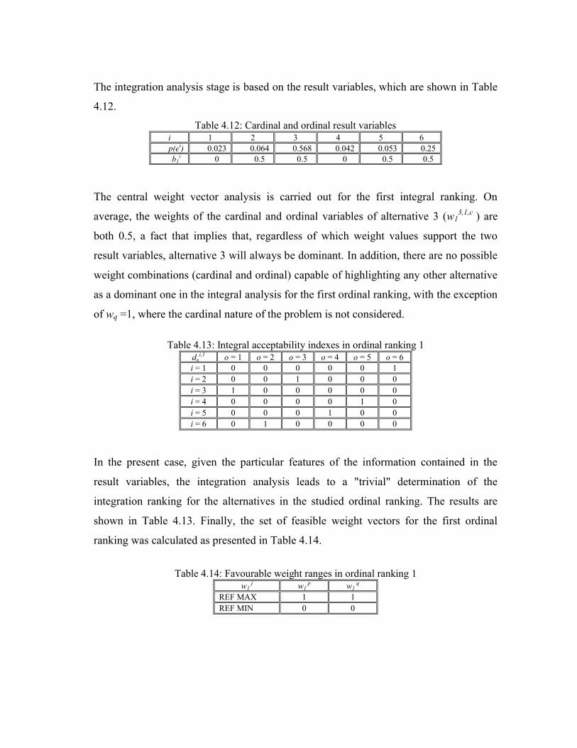
The integration analysis stage is based on the result variables, which are shown in Table
4.12.
Table 4.12: Cardinal and ordinal result variablesi 1 2 3 4 5 6p(ei) 0.023 0.064 0.568 0.042 0.053 0.25b1
i 0 0.5 0.5 0 0.5 0.5
The central weight vector analysis is carried out for the first integral ranking. On
average, the weights of the cardinal and ordinal variables of alternative 3 (w13,1,c ) are
both 0.5, a fact that implies that, regardless of which weight values support the two
result variables, alternative 3 will always be dominant. In addition, there are no possible
weight combinations (cardinal and ordinal) capable of highlighting any other alternative
as a dominant one in the integral analysis for the first ordinal ranking, with the exception
of wq =1, where the cardinal nature of the problem is not considered.
Table 4.13: Integral acceptability indexes in ordinal ranking 1 do
i,1 o = 1 o = 2 o = 3 o = 4 o = 5 o = 6i = 1 0 0 0 0 0 1i = 2 0 0 1 0 0 0i = 3 1 0 0 0 0 0i = 4 0 0 0 0 1 0i = 5 0 0 0 1 0 0i = 6 0 1 0 0 0 0
In the present case, given the particular features of the information contained in the
result variables, the integration analysis leads to a "trivial" determination of the
integration ranking for the alternatives in the studied ordinal ranking. The results are
shown in Table 4.13. Finally, the set of feasible weight vectors for the first ordinal
ranking was calculated as presented in Table 4.14.
Table 4.14: Favourable weight ranges in ordinal ranking 1w1
j w1 p w1
q
REF MAX 1 1REF MIN 0 0

The indicators supplied by IAM allowed establishing that alternative 3 was the most
feasible and useful one, since it presents the best values for the two result variables
(cardinal and ordinal).
The results demonstrated the significant advantages of IAM in the decision making
process. This method allowed the company to express and properly use its expertise in
an orderly and technical way.
4.5. Conclusions
IAM was conceived to deal with problems that have a significant complexity, due to the
necessity of including aspects that cannot be quantified in the objective function of the
combinatorial problems.
IAM is carried out in four stages: the first one establishes the type of problem (cardinal
and/or ordinal) and its stochastic or deterministic nature. In the second stage the
alternatives are selected considering optimization criteria and variability of the cardinal
variables, an analysis in which Monte Carlo Simulation and probability elements are
employed as optimization techniques. In the third stage, the alternatives are further
analyzed by means of SMAA-O and probability elements. In the final stage the
alternatives are analyzed again in both ordinal and cardinal aspects using a transformed
version of deterministic SMAA and probability elements. Conclusions are finally drawn
from the indicators obtained in the three last stages.
The technique allows a deeper analysis of the problem, as far as it provides multiple
indicators that describe the ordinal and cardinal information concerning each of the
alternatives. It must be pointed, however, that in applying IAM to practical cases, the
number of a study’s alternatives needs to be restricted as to make the technique
applicable.

As for the future, three areas of possible further research can be recognized: in the first
place, reliability and validity of a more general methodology that enables researchers to
define the problem and determine the relevance of variables and data collection
processes. In the second place, the identification of new indicators that strengthen the
methodology; and last, the application of the methodology on other optimization
problems in a more general context than the one considered in this article.
4.6. References
Albaum, G. (1997), The Likert scale revisited: an alternative version. Journal of the
Market Research Society 39 (2) 331-348.
Bana E Costa, C.A. (1986), A multicriteria decision-aid methodology to deal with
conflicting situations on the weights. European Journal of Operational Research
26 22-34.
Bana E Costa, C.A. (1988), A methodology for sensitivity analysis in three-criteria
problems: A case study in municipal management, European Journal of
Operational Research 33 159-173.
Beamon, B.M. (1998), Supply chain design and analysis: models and methods,
International Journal of Production Economics 55(3) 281-294.
Birge, J.R. Quasi-Monte Carlo methods for option evaluation. Technical Report,
Department of Industrial and Operations Engineering, University of Michigan
(Ann Arbor, MI), 1994.
Birge, J.R., Louveaux, F.V. Introduction to Stochastic Programming. Springer-Verlag,
New York, 1997.
Brown, P.A., Gibson, D.F. (1972), A quantified model for facility site selection applied
to a multipoint location problem. AIIE Transactions 4 1-10.
Churchill, G.A. (1979), A paradigm for developing better values of marketing
constructs. Journal of Marketing Research 16 64-74.
David, H.A. Order Statistics. Wiley, New York; 1970.

Durbach, I. (2006), A simulation-based test of stochastic multicriteria acceptability
analysis using achievement functions. European Journal of Operational Research
170(3) 923-934.
Dyer, J.S. Remarks on the Analytical Hierarchy Process. Management Science 1990; 3;
249-258.
Figueiredo, O., Guimaraes, P. (2003), A tractable approach to the firm location decision
problem. The Review of Economics and Statistics, Cambridge 85(1) 201-204.
García, R.G., Aráoz, J.A., Palacios, F. (2005a ), The integral analysis method. Reports of
the Departament d’EIO. Sección Informática, Universitad Politécnica Catalunya
DR, 07.
García, R.G., Caro, M.P., Díaz, H., Sánchez, L.L., Carrillo, M.H. (2004), Metodología
marco de referencia para la localización de instalaciones, Ingeniería y Universidad
8(2) 139-157.
García, R.G., Palacios, F., Aráoz, J.A. (2005b ), Implementation of the integral analysis
method in strategic supply chain. Reports of the Departament d’EIO. Secció
Informática, Universitad Politécnica Catalunya DR, 08.
Geoffrion, A.M., Graves, G. (1974), Multicommodity distribution system design by
Benders decomposition, Management Science 20(5) 822- 844.
Geoffrion, A.M., Power, R.F. (1995), Twenty years of strategic distribution system
design: An evolutionary perspective. (Implementation in OR/MS: An evolutionary
view). Interfaces 25(5) 105-128.
Greco, S., Matarazzo, B., Slowinski, R. (2001), Rough sets theory for multicriteria
decision analysis. European Journal of Operational Research 129(1) 1-47.
Greco, S., Matarazzo, B., Slowinski, R. 2005. Decision rule approach. Chapter 13
[in]: J.Figueira, S.Greco and M.Ehrgott (eds.), Multiple Criteria Decision
Analysis: State of the Art Surveys, Springer-Verlag, New York; 2005. p. 507-562.
Hokkanen, J., Lahdelma, R., Miettinen, K., Salminen, P. (1998) Determining the
implementation order of a general plan by using a Multicriteria Method. Journal of
Multi-Criteria Decision Analysis 7 273-284.
Hokkanen, J., Lahdelma, R., Salminen, P. (1999), A multiple criteria decisions model
for analyzing and choosing among different development patterns for the Helsinki
Cargo Harbor, Socio-Economic Planning Sciences 33 1-23.
Hokkanen, J., Lahdelma, R., Salminen, P. (2000), Multicriteria decision support in a
technology competition for cleaning polluted soil in Helsinki. Journal of
Environmental Management 60(4) 339-348.
Kall, P., Wallace, S.W. Stochastic Programming. John Wiley & Sons, New York; 1994.
Keeney, R.L., Raiffa, H. Decisions with Multiple Objectives: Preferences and Value
Tradeoffs. Wiley, New York; 1976.
Khumawala, B.M. (1972), An efficient branch and Bound Algorithm for the warehouse
location problem. Management Science 18 718-732.
Lahdelma, R., Hokkanen, J., Salminen, P. (1998), SMAA - Stochastic Multiobjective
Acceptability Analysis. European Journal of Operational Research 106(1) 137-143.
Lahdelma, R., Makkonen, S., Salminen, P. (2006), Multivariate Gaussian criteria in
SMAA. European Journal of Operational Research 170(3) 957-970.
Lahdelma, R., Miettinen, K., Salminen, P. (2003), Ordinal criteria in Stochastic
multicriteria acceptability analysis. European Journal of Operational Research 147
117-127.
Lahdelma, R., Salminen, P. (2001), SMAA- 2: Stochastic multicriteria acceptability
analysis for group decision making. Operations Research 49(3) 444-454.
Lahdelma, R., Salminen, P. (2006a), Classifying alternatives in SMAA using cross
confidence factors. European Journal of Operational Research 170(1) 228-240.
Lahdelma, R., Salminen P. (2006b ), Stochastic multicriteria acceptability analysis using
the data envelopment model. European Journal of Operational Research 170(1)
241-252.
Lahdelma, R., Salminen, P., Hokkanen, J. (2002), Locating a waste treatment facility by
using stochastic multicriteria acceptability analysis with ordinal criteria. European
Journal of Operational Research 142 345-356.
Martin, R.K. Large Scale Linear and Integer Optimization: A unified approach. Kluwer
Academic Publishers, Boston; 1999.
Miettinen, K., Salminen, P. (1999), Decision – aid for discrete multiple criteria decision
making problems with imprecise data. European Journal of Operational Research
119 50-60.
Pooley, J. (1994) Integrated production and distribution facility planning at Ault Foods.
Interfaces 24(4) 113-121.
Rietveld, P. Multiple Objective Decision Methods and Regional Planning. Studies in
Regional Science and Urban Economics; Volume 7, North Holland Publishing
Company. North-Holland, Amsterdam; 1980.
Rietveld, P., Ouwersloot, H. (1992), Ordinal data in multicriteria decision making, a
stochastic dominance approach to sitting nuclear power plants. European Journal
of Operational Research 56(2) 249-262.
Saaty, T.L. The Analytic Hierarchy Process. McGraw-Hill, New York; 1980.
Schrijver, A. Theory of Linear and Integer Programming. Wiley, New York; 1986.
Slowinski, R., Greco, S., Matarazzo, B. 2005. Rough set based decision support.
Chapter 16 [in]: E.K. Burke and G. Kendall (eds.), Search Methodologies:
Introductory Tutorials in Optimization and Decision Support Techniques,
Springer-Verlag, New York; 2005. p. 475-527.
Steuer, R. Multiple Criteria Optimization: Theory, Computation and applications. Wiley,
New York; 1986.
Tervonen T., Lahdelma R. (2007), Implementing Stochastic Multicriteria Acceptability
Analysis. European Journal of Operational Research 178(2) 500-513.
Torres, S., García, R.G., Quintero, J. (2005), Formas de CONTRATACIÓN de los
servicios de urgencias: una APROXIMACIÓN desde la economía de los costos de
transacción. Economía Institucional 7(12) 97-127.
Vidal C.J., Goetschalckx M. (1997), Strategic production-distribution models: A critical
review with emphasis on global supply chain models. European Journal of
Operational Research 98 1-18.
Vidal, C.J., Goetschalckx, M. (2000), Modeling the effect of uncertainties on global
logistics systems. Journal of Business Logistics 21(1) 95-120.
Vincke, Ph. Multicriteria Decision –Aid. Wiley, New York; 1992.

Watson, S.R., Buede, D.M. Decision Synthesis: The principles and practice of decision
analysis. Cambridge University Press; 1987.
Zeleny, M. Multiple Decision Making. McGraw-Hill, New York; 1982.

INTRODUCTION REFERENCES
Aikens , C.H. (1985), Facility location models for distribution planning. European
Journal of Operational Research 22 263-279.
Artz, K.W., Norman, P.M.. (2002), Buyer-supplier contracting: contract choice and ex-
post negotiation costs. Journal of Managerial Issues 14(4) 399-417.
Bhatnagar, R., Chandra, P., Goyal, S.K. (1993), Models for multi-plant coordination.
European Journal of Operational Research 67 141-160.
Beamon, B.M. (1998), Supply chain design and analysis: models and methods.
International Journal of Production Economics 55(3) 281-294.
Brennan, C.D. (1998), Integrating the healthcare supply chain. Healthcare Financial
Management 52 (1) 31-34.
Coase, R. H. (1937), The nature of the firm. Económica 4 (16) 386-405.
Cohen, M.A., Lee, H.L. (1988), Strategic analysis of integrated production-distribution
systems: Models and methods. Operations Research 36 216-228.
Dwyer, F.R., Schurr, P., Oh, S. (1987), Developing buyer-seller relationships. Journal of
Marketing 51 (2) 11-27
Geoffrion, A.M., Power, R.F. (1995), Twenty years of strategic distribution system
design: An evolutionary perspective. (Implementation in OR/MS: An evolutionary
view). Interfaces 25(5) 105-128.
Giannakis, M., Croom. S. (2004), Toward the development of a supply chain
management paradigm: a conceptual framework. Journal of Supply Chain
Management 40 (2) 27-37.
Goetschalckx M., Vidal C.J., Dogan K. (2002), Modeling and design of global logistic
system: A review of integrated strategic and tactical models and design algorithms.
European Journal of Operational Research 143 (1) 1-18.
Grover, V., Malhotra, M.K. (2003), Transaction cost framework in operations and
supply Chain management research – Theory and measurement. Journal of
Operations Management 21 (4), 457-473.

Gu, Q. Multiple-period Supply Chain Contract Modeling with Dynamic Stochastic and
Price-elastic Demand. Doctoral Dissertation. Florida Atlantic University, Boca
Raton 2001.
Harrison, T.P., Hau, L.L., Neale, J.J., (Eds.). The Practice of Supply Chain
Management: Where Theory and Application Converge. Kluwer Academic
Publishing, Boston, 2003.
Heide, J.B. (1994), Interorganizational governance in marketing channels. Journal of
Marketing 58 (1) 71-85.
Johnson, J.C., Wood, D.F., Wardlow, P.R., Murphy, Jr. Contemporary Logistics. Simon
and Schuster, New York, 1999.
Kim, K., Frazier, G.L. (1996), A typology of distribution channel system: a contextual
approach. International Marketing Review 13 (1) 19-32.
Lambert, D. M., Cooper, M.C., Pagh, J.D. (1998), Supply chain management:
implementation issues and research opportunities. The international Journal of
Logistics 9 (2) 1-19.
Lambert, D.M, García-Dastugue, S., Croxton, K.L. (2005), An evaluation of process-
oriented supply chain management frameworks. Journal of business Logistics 26
(1) 25-51.
Lummus, R.R., Vokurka, R.J. (1999), Defining supply chain management: a historical
perspective and practical guidelines. Industrial Management & Data Systems 99
(1) 11-17.
McKone-Sweet, K., Hamilton, P., Willis, S. (2005), The ailing healthcare supply Chain:
a prescription for change. Journal of Supply Chain Management 40 (1) 4-17.
Moriarty, R.T., Moran, U. (1990), Managing hybrid marketing systems. Harvard
Business Review 68 (Nov.-Dec.) 146-155.
O’Toole, T., Donaldson. B. (2000), Managing buyer-supplier relationships archetypes.
Irish Marketing Review 13 (1) 12-20.
Palay, T.M. Comparative institutional economics: the governance of rail Freight
contracting. Journal of Legal Studies 1984; 13 (June): 265-288.

Paulraj, S.C. A. Towards a unified theory in supply chain management: critical
constructs and their effect on performance. Bussiness Administration Doctoral
dissertation. Cleveland State University, Cleveland, 2002.
Porter, M.E. (1987), Managing value – from competitive advantage to corporate
strategy. Harvard Business Review 65 (3) 43-60.
Prahalad, C.K., Hamel, G. (1990), The core competence of the corporation. Harvard
Business Review (May-June); 79-91.
Quinn, F. J. (1997), What’s the buzz?. Logistics Management 36 (2) 43-46.
Shapiro, J.F. (2001), Modelling the Supply Chain. Duxbury Thomson Learning Inc.,
Pacific Grove (CA).
Shin, H., Collier, D., Wilson, D.D. (2000), Supply management orientation and
supplier/buyer performance. Journal of Operations Management 18(3) 317-333.
Tan, K.C. (2001), A framework of supply chain management literature. European
Journal of Purchasing and Supply Management 7 (1) 39-48.
Thomas D., Griffin, M.C. (1996), Coordinate supply chain management. European
Journal of Operational Research 94 1-15.
Tsay, A.A., Nahmias, S., Agrawal, N. Modeling Supply Chain Contracts: A Review,
Quantitative Modelling for Supply Chain Management. Kluwer Academic
Publishers, Norwell (MA); 1999.
Vidal C.J., Goetschalckx M. (1997), Strategic production-distribution models: A critical
review with emphasis on global supply chain models. European Journal of
Operational Research 98 1-18.
Weng, Z.K. (1995), Modeling quantity discounts under general price–sensitive demand
functions: Optimal policies and relationships. European Journal of Operational
Research 86 (2) 300-314.
Williamson, O.E. Markets and hierarchies; analysis and antitrusth implications. New
York; 1975
______________. The Economic institutions of capitalism. New York; 1985.
______________(1991), Comparative economic organization: The analysis of discrete
structural alternatives. Administrative Science Quarterly 36 (2) 269-296.

______________(1993), Calculativeness; trust and economic organization. Journal of
Law and Economics 36 (2) 453-486.