integrated approach to alm, risk budgeting and alpha

Integrated Approach to ALM, Risk Budgeting and AlphaDetermining an appropriate risk budget for active management has historically taken place without much regard to the determination of the investment strategy. Yet adding active management to the strategy has implications for the absolute risk/return trade-off that lies at the heart of finding the right long-term asset mix in the first place. In this paper we show how the risk budget can be determined as integral part of an ALM study, providing internal consistency between the long and short term aspects of investment policy. The analysis also allows for separation of α and β exposures.

Multi-Asset Solutions Research Papers - Issue 2

For institutional and adviser use only

The concept of “risk budget” has been used in recent years to provide a lodestar for active management of an investment portfolio. The risk budget is traditionally expressed in terms of tracking error relative to a long-term strategic benchmark, which in turn is determined by an Asset-Liability Management (ALM) study. But there usually is a disconnect between the two, as the risk budget is determined exogenously, without regard to the strategic benchmark or the ALM study.

An ALM study will determine the strategic benchmark by finding the optimal trade-off between absolute risk and return, or functions thereof. For a defined benefit pension fund, for instance, the absolute risk/return trade-off might consist of minimising the present value of contributions in the worst case, while ensuring maximum expected funding ratio. The strategic benchmark that follows will embody this trade-off.

Yet by adding active management, and thus tracking error to this benchmark, the trade-off itself is altered. It is therefore important to quantify the impact of active management on the absolute risk/return trade-off. In fact, given the crucial nature of this trade-off, the determination of how much tracking error one can add should be done within the context of an ALM study, and not as an afterthought.

The risk budget and strategic benchmark are interrelated: by adding a risk budget, the strategic benchmark should change. This is because the risk profile of the allocations changes, which in turn affects the trade-off. We can also calculate the information ratio that is required to make up for the additional risk that has been introduced.

There is also a benefit from separating α and β. Traditionally an ALM study has only resulted in finding an optimal mix of long-term β exposures. Given that equity and bond market βs can be modelled with more long-term significance than α, this was a reasonable approach to take1. Now however we can incorporate largely uncorrelated α at the ALM stage into the portfolio as well.

In section 2 we present the conceptual theoretical setting for this paper. We show in particular how in ALM context a strategic benchmark (for β exposure) in combination with a risk budget w(for uncorrelated α) can be derived.

1 By definition α is uncorrelated with β, and can come from a multitude of idiosyncratic sources. This makes the modelling of α much trickier and less reliable than β.

Introduction

1

First Sentier Investors Multi-Asset Solutions Research Papers Issue 2

PassiveVolatility however is not constant over time. It varies in different periods as the economic cycle goes through ups and downs, and markets are perturbed by events. To show this we calculated the annualised volatility of the S&P 500 index using four different time windows: rolling over 12, 24 and 60 months, as well as an expanding window from 1980 until the last data point ending February 2012.

Figure 1

BAD

Objective

GOOD

Acceptable

Unacceptable

Risk

crit

erio

n

S-curve

MRP

ARP

Source: First Sentier Investors

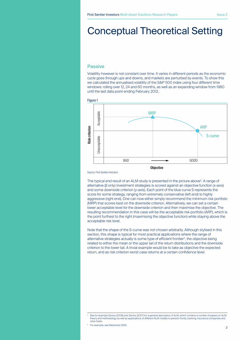
The typical end result of an ALM study is presented in the picture above2. A range of alternative (β only) investment strategies is scored against an objective function (x-axis) and some downside criterion (y-axis). Each point of the blue curve S represents the score for some strategy, ranging from extremely conservative (left end) to highly aggressive (right end). One can now either simply recommend the minimum risk portfolio (MRP) that scores best on the downside criterion. Alternatively, we can set a certain lower acceptable level for the downside criterion and then maximise the objective. The resulting recommendation in this case will be the acceptable risk portfolio (ARP), which is the point furthest to the right (maximising the objective function) while staying above the acceptable risk level.

Note that the shape of the S-curve was not chosen arbitrarily. Although stylised in this section, this shape is typical for most practical applications where the range of alternative strategies actually is some type of efficient frontier3, the objective being related to either the mean or the upper tail of the return distributions and the downside criterion to the lower tail. A trivial example would be to take as objective the expected return, and as risk criterion worst case returns at a certain confidence level.

2 See for example Zenios (2006) and Zenios (2007) for a general description of ALM, which contains a number of papers on ALM theory and methodology as well as applications of different ALM models to pension funds, banking, insurance companies and other fields.

3 For example, see Markowitz (1991).

Conceptual Theoretical Setting

2


ActiveHaving established the appropriate β for the portfolio, in a traditional setting the ALM study would be concluded at this stage. The setting of a risk budget, if any, would take place entirely disjointed from this exercise4. That approach is far from optimal, and the risk budget should be taken into account as it impacts the long-term strategic risk profile.

We employ a two-step approach to overcome this:

i) Overlay an uncorrelated asset with volatility = σ0 and α = 0 and investigate the effect this has on the strategy and the risk/return trade off.

ii) Determine the level of α necessary to compensate for the additional volatility.

By starting off with the admixture of an uncorrelated asset with zero α and with volatility σ0 we can avoid having to make assumptions on manager α. First of all one should realise that adding the overlay introduces new volatilities on both the outcomes for the objective and the downside criterion. This effect is conceptually represented by the circle areas5 around the S-curve in the picture below. The radius of these circles is stylised as σ0. Now connecting the lower ends of this family of circles as the new downside levels leads to a transformation of the S-curve to a new curve, labeled as T0,σ0(S). The reason the T0,σ0(S) in broad terms results in a downward shift from the original S-curve is that the assumption of zero alpha does not affect the expected value of the objective function, but it does worsen the worst-case outcome. In case the objective function is not an expected value, but for instance a percentile in the upper tail of a distribution, the shift from the S-curve to T0,σ0(S) will not be a simple downward translation, but also be subject to more horizontal movement in the graph.

Objective

Risk

crit

erio

n

σ0T0,σ0

(S)-curv e

S-curve

BAD GOOD

Acceptable

Unacceptable


It is clear that the setting changes now. The previous MRP or ARP recommendations turn out to be irrelevant or at least suboptimal since they were derived from the S-curve, which has been superseded by the T0,σ0(S)-curve.

4 For example, see Engstrom (2008), Siegel (2003) and Anson (2004).5 The circular shape is used here only for illustrative purposes. In any given practical case the shape will be different.

3


The new MRP and ARP are shown below.

BAD

Objective

GOOD

UNAC

CEPT

ABLE

ACCE

PTAB

LE

Risk

crit

erio

n

T0,σ0(S)-curv e

T0,σ0(S)

S0

ARP S

MRP S

MRPMRP

ARP = T0,σ0(S0)

T0,σ0(S)

BAD

Objective

GOOD

UNAC

CEPT

ABLE

ACCE

PTAB

LE

Risk

crit

erio

n

ARP = T 0,σ0(S0)

T0,σ0(S)

Tα,σ0(S0)-curve

Tα0,σ0(S0)

S0


Note that the T-curve was derived from the S-curve by adding an uncorrelated asset to the original strategies. In terms of its composition the new MRPT will typically be derived from a strategy close to the previous MRPS , but this certainly does not hold for the new ARPTS), derived from a certain strategy S0, which in general will be considerably more conservative than the original ARPS. One can easily see this also by their different positions on the relevant curves.

Although by definition the new and the old ARP both have the same downside level, it is clear that in terms of the objective the old ARP is superior as it lies further to the right in the graph. This is due to our zero α assumption for the overlay, which has the net effect of adding volatility without any added value.

The next step is to add α to the overlay. A positive α will move the new ARP to the right and upwards, since it will improve the situation on the downside and will also help in achieving the objective. A negative α will do exactly the opposite. The green curve, labelled Tα0,σ0(S0) in the next picture represents this effect for a range of αs.

BAD

Objective

GOOD

UNAC

CEPT

ABLE

ACCE

PTAB

LE

Risk

crit

erio

n

T0,σ0(S)-curv e

T0,σ0(S)

S0

ARP S

MRP S

MRPMRP

ARP = T0,σ0(S0)

T0,σ0(S)

BAD

Objective

GOOD

UNAC

CEPT

ABLE

ACCE

PTAB

LE

Risk

crit

erio

n

ARP = T 0,σ0(S0)

T0,σ0(S)

Tα,σ0(S0)-curve

Tα0,σ0(S0)

S0


4


We highlight one particular point on this curve, namely the point where the value for the objective is equal to the original ARPS. This point, labeled Tα0,σ0(S0), shows superior behaviour with respect to the risk criterion. Therefore, if active management is able to deliver α0 excess return within a tracking error of σ0, or, equivalently an Information Ratio of α0/σ0, it is worthwhile to have S0 as strategy and add an overlay with σ0 volatility, instead of sticking passively to the original (more aggressive) ARPS. In each specific case one can assess the level of this required Information Ratio and take decisions on that basis.

Note that the portfolio Tα0,σ0(S0) is in fact the point on the Tα0,σ0(S)-curve that corresponds to the original strategy S0, as shown in the graph below.

BAD

Objective

GOOD

UNAC

CEPT

ABLE

ACCE

PTAB

LE

Risk

crit

erio

n

ARP = T 0,σ0(S0)

T0,σ0(S)

T α,σ 0(S 0

)-curve

Tα0,σ0(S0)S0

T0,σ0

(S)-curve Tα0,σ0

(S)-curve

BAD

Objective

GOOD

UNAC

CEPT

ABLE

ACCE

PTAB

LE

Risk

crit

erio

n

ARP = T 0,σ0(S0)

T0,σ0(S)

T α,σ 0(S 0

)-curveT α,0

(S 0)-curve

Tα0,0(S0)Tα0,0(S0)

S0S0T0,σ0(S)

MRPMRP

T0,σ0

(S)-curve Tα0,σ0

(S)-curve Tα0,0(S)-curve

Tα0,σ0(S0)Tα0,σ0(S0)


In fact, there is a continuum of curves that we can calculate, depending on one of the parameters α, σ and strategies S0.

BAD

Objective

GOOD

UNAC

CEPT

ABLE

ACCE

PTAB

LE

Risk

crit

erio

n

ARP = T 0,σ0(S0)

T0,σ0(S)

T α,σ 0(S 0

)-curve

Tα0,σ0(S0)S0

T0,σ0

(S)-curve Tα0,σ0

(S)-curve

BAD

Objective

GOOD

UNAC

CEPT

ABLE

ACCE

PTAB

LE

Risk

crit

erio

n

ARP = T 0,σ0(S0)

T0,σ0(S)

T α,σ 0(S 0

)-curveT α,0

(S 0)-curve

Tα0,0(S0)Tα0,0(S0)

S0S0T0,σ0(S)

MRPMRP

T0,σ0

(S)-curve Tα0,σ0

(S)-curve Tα0,0(S)-curve

Tα0,σ0(S0)Tα0,σ0(S0)

4 This is based on a separate calculation using weekly data to capture shorter-term movements.5 Essentially, these are correlations calculated using three and six pairs of data, and therefore are not statistically significant.

Using weekly data we see negative correlations prevailing, approaching –0.8.

5


Maximum Risk BudgetAnother question we can answer using this methodology is whether there exists a maximum risk budget. Going back to the zero α situation for the sake of prudence one can draw T-curves for increasing volatilities σ for the overlay. At a certain point the T-curve will end up tangent to the acceptable level. Going beyond that point will lead to a situation where none of the T-curve portfolios satisfies the risk tolerance criterion. The T-curve will then be entirely below the acceptable level.

Hence the maximum allowed volatility σmax is reached when T0,σ(S) is tangent to acceptable level with only one portfolio satisfying the risk criterion. This portfolio is then the MRP and the ARP at the same time for T0,σmax(S).

7

BAD

Objective

GOOD

UNA

CCEP

TABL

EAC

CEPT

ABLE

Risk

crit

erio

n ARP S

T0,σmax(S)-curve

σma x

MRP = ARPT0,σmax(S) T0,σmax

(S)

BAD

Objective

GOOD

UNA

CCEP

TABL

EAC

CEPT

ABLE

Risk

crit

erio

n

S-curve

MRP SMRP S

T0,σ0(S)-curve

Tα*,σ0(S0)Tα*,σ0(S0)Tαmin ,σ0

( )Tαmin ,σ0( )

S0S0

T0,σ0(S)

MRPMRP

T0,σ0(S)

MRPMRP


Set of passive portfolios below acceptable risk levelSo far we have assumed that an ARP exists. However, this does not hold when the S-curve lies below the acceptable risk level for the entire set of investment strategies as in the graph below. In this case the risk criterion is not met by any of the strategies. Using passive management only, the analysis would be concluded by selecting the MRP, which is the strategy closest to the acceptable risk level.

7

BAD

Objective

GOOD

UNA

CCEP

TABL

EAC

CEPT

ABLE

Risk

crit

erio

n ARP S

T0,σmax(S)-curve

σma x

MRP = ARPT0,σmax(S) T0,σmax

(S)

BAD

Objective

GOOD

UNA

CCEP

TABL

EAC

CEPT

ABLE

Risk

crit

erio

n

S-curve

MRP SMRP S

T0,σ0(S)-curve

Tα*,σ0(S0)Tα*,σ0(S0)Tαmin ,σ0

( )Tαmin ,σ0( )

S0S0

T0,σ0(S)

MRPMRP

T0,σ0(S)

MRPMRP


6


7 This is based on historical data and does not include any stress-testing.

By adding active management however, it is possible to find a strategy that still meets the risk criterion. Again, we start by adding an uncorrelated asset with volatility σ0 and zero α. The resulting T0,σ0(S)-curve lies even further below the acceptable risk level than the original S-curve. The choice of the optimal investment strategy now depends on one’s confidence in active management, with minimal dependence on active management resulting from the MRP on the T-curve. Starting from this point, we can calculate the amount of alpha αmin needed to reach the acceptable risk level. This is shown by the point Tαmin,σ0(MRPT0,σ (S)). However, if it is expected that more α can be generated by active management, a less conservative strategy can be used instead, allowing for a higher upside potential. This is shown by the point Tα*,σ0(S0), which lies on the acceptable risk level and to the right of point Tαmin,σ0(MRPT0,σ (S)).

HedgingThe final topic that we will address in this section is hedging. Hedging has the effect of lowering risk on the one hand, but lowering the objective on the other hand as well, assuming that hedging has a cost. The S-curve will shift up and to the left in this case. This is shown in the tripod below, where it is contrasted with the effect of adding alpha, which improves both the worst case outcome as well as the upside potential.

Increased Hedge Increased Alpha

Increased Tracking Error budget

Because hedging lowers the downside risk (the graph shifts upward), the ARP on the new curve (H-curve) will be less conservative compared to the ARP on the original S-curve. Using a higher hedge ratio implies that at the acceptable risk level, a higher objective value can be realised by applying a hedging strategy. As can be seen from the graph below, the ARP shifts to the right with a higher objective value.

7


BAD

Objective

GOOD

UNA

CCEP

TABL

EAC

CEPT

ABLE

Risk

crit

erio

n

MRP SARP S

S-Curve

H-Curve

MRP H

ARP H

BAD

Objective

GOOD

UNA

CCEP

TABL

EAC

CEPT

ABLE

Risk

crit

erio

n

MRP S0

ARP

Acceptable risk strategiesFixed Risk Budget σmax

25% HR50% HR

75% HR

IncreasedAlpha

Increased Hedge

Increase TrackingError budget

S-curve


The H-curve can obviously be used as the new starting point to apply the risk budgeting approach as presented earlier. The next figure shows acceptable risk portfolios for increasing hedge ratios, based on a fixed risk budget. Here, S0 is the portfolio that corresponds to the ARP on some T-curve using a zero hedge ratio, while for instance the 50% HR portfolio is the strategy corresponding to the ARP on that same T-curve using a 50% hedge ratio.

BAD

Objective

GOOD

UNA

CCEP

TABL

EAC

CEPT

ABLE

Risk

crit

erio

nMRP S

ARP S

S-Curve

H-Curve

MRP H

ARP H

BAD

Objective

GOOD

UNA

CCEP

TABL

EAC

CEPT

ABLE

Risk

crit

erio

n

MRP S0

ARP

Acceptable risk strategiesFixed Risk Budget σmax

25% HR50% HR

75% HR

IncreasedAlpha

Increased Hedge

Increase TrackingError budget

S-curve


8


The graph below shows the combined effect of hedging and adding alpha.

BAD

Objective

GOOD

UNA

CCEP

TABL

EAC

CEPT

ABLE

Risk

crit

erio

nAcceptable Risk Strategy

Minimum Risk Stategy

β-only -curve

β+α+LH -curve

Adding αLiabilityHedging


Although not too hard to visualise in the above stylised form, putting this concept into practice is not entirely straightforward. In order to make the above concept work and showing its applicability in a practical setting, we will have to go through a complete ALM analysis.

9


Anson, M., “Strategic versus Tactical Asset Allocation”, Journal of Portfolio Management, Winter 2004.

Boender, G., Dert, C., Heemskerk, F. and Hoek, H., “A Scenario Approach of ALM, Handbook of Asset and Liability Management”, Volume 2: Applications and Case Studies, Chapter 18, 2007.

Engstrom, S., Grottheim, R., Norman, P. and Ragnartz, C., “Alpha-Beta-Separation: From Theory to Practice”, available at SSRN: http://ssrn.com/abstract=1137673, 2008.

Markowitz, H.M., Portfolio Selection: “Efficient Diversification of Investments”, Second Edition, Blackwell, 1991.

Siegel, B. and Barton Waring, M., “The Dimensions of Active Management”, Journal of Portfolio Management, Spring 2003.

Tsay, R., “Analysis of Financial Time Series”, 2nd Edition, John Wiley & Sons, 2005.

Zenios, S.A. and Ziemba, W., “Handbook of Asset and Liability Management”, Volume 1: Theory and Methodology, Elsevier Publishers, 2006.

Zenios, S.A. and Ziemba, W., “Handbook of Asset and Liability Management”, Volume 2: Applications and Case Studies, Elsevier Publishers, 2007.

References

10


Important InformationThis material has been prepared and issued by First Sentier Investors (Australia) IM Ltd (ABN 89 114 194 311, AFSL 289017) (Author). The Author forms part of First Sentier Investors, a global asset management business. First Sentier Investors is ultimately owned by Mitsubishi UFJ Financial Group, Inc (MUFG), a global financial group. A copy of the Financial Services Guide for the Author is available from First Sentier Investors on its website.This material contains general information only. It is not intended to provide you with financial product advice and does not take into account your objectives, financial situation or needs. Before making an investment decision you should consider, with a financial advisor, whether this information is appropriate in light of your investment needs, objectives and financial situation. Any opinions expressed in this material are the opinions of the Author only and are subject to change without notice. Such opinions are not a recommendation to hold, purchase or sell a particular financial product and may not include all of the information needed to make an investment decision in relation to such a financial product.To the extent permitted by law, no liability is accepted by MUFG, the Author nor their affiliates for any loss or damage as a result of any reliance on this material. This material contains, or is based upon, information that the Author believes to be accurate and reliable, however neither the Author, MUFG, nor their respective affiliates offer any warranty that it contains no factual errors. No part of this material may be reproduced or transmitted in any form or by any means without the prior written consent of the Author.Copyright © First Sentier Investors (Australia) Services Pty Ltd 2020. All rights reserved.

11


integrated approach to alm, risk budgeting and alpha

Documents