integrated decision making in global supply chains...
TRANSCRIPT
INTEGRATED DECISION MAKING IN GLOBAL SUPPLY CHAINS AND NETWORKS
by
Ozlem Arisoy
B.S. in Industrial Engineering, Bogazici University, 2003
M.S. in Industrial Engineering, University of Pittsburgh, 2004
Submitted to the Graduate Faculty of
the School of Engineering in partial fulfillment
of the requirements for the degree of
Doctor of Philosophy
University of Pittsburgh
2007

ii
UNIVERSITY OF PITTSBURGH
SCHOOL OF ENGINEERING
This dissertation was presented
by
Ozlem Arisoy
It was defended on
July 6, 2007
and approved by
Dissertation Director: Bopaya Bidanda, Professor, Industrial Engineering Department
Dissertation Co-Director: Larry J. Shuman, Professor, Industrial Engineering Department
Brady Hunsaker, Assistant Professor, Industrial Engineering Department
Ravindranath Madhavan, Associate Professor, Business Administration
Kim LaScola Needy, Associate Professor, Industrial Engineering Department

iii
Copyright © by Ozlem Arisoy 2007
iv
One of the more visible and often controversial effects of globalization is the rising trend in
global sourcing, commonly referred to as outsourcing, offshoring and offshore outsourcing.
Today, many organizations experience the necessity of growing globally in order to remain
profitable and competitive. This research focuses on the process that organizations undergo in
making strategic decisions of whether or not to go offshore, and then on the location and volume
of these offshore operations.
This research considers the strategic decision of offshoring and sub-divides it into two
components: analysis of monetary benefits and evaluation of intangible variables. In this
research, these two components are integrated by developing an analytical decision approach that
can incorporate quantitative and qualitative factors in a structure based on multiple solution
methodologies. The decision approach developed consists of two phases which concurrently
assess the offshoring decision by utilizing mixed integer programming and multi-attribute
decision modeling, specifically using Analytic Network Process, followed by multi-objective
optimization and tradeoff analysis. The decision approach is further enhanced by employing
engineering economic tools such as life cycle costing and activity based costing. As a result, the
approach determines optimal offshoring strategies and provides a framework to investigate the
optimality of the decisions with changing parameters and priorities.
INTEGRATED DECISION MAKING IN GLOBAL SUPPLY CHAINS AND NETWORKS
Ozlem Arisoy, PhD
University of Pittsburgh, 2007

v
The applicability, compliance and effectiveness of the developed integrated decision
making approach is demonstrated on two real life cases in two different industry types. Through
empirical studies, different dimensions of offshoring decisions are examined, classified and
characterized within the framework of the developed decision approach. The solutions are
evaluated by their value, level of support and relevance to the decision makers. The utilization of
the developed systematic approach showed that counterintuitive decisions may sometimes be the
best strategy.
This study contributes to the literature with a comprehensive decision approach for
determining the most advantageous offshoring location and distribution strategies by integrating
multiple solution methodologies. This approach can be adapted in the corporate world as a tool
to improve global perspective and direction.
vi
TABLE OF CONTENTS
PREFACE.................................................................................................................................... xiv
1.0 INTRODUCTION .............................................................................................................. 1
1.1 MOTIVATION............................................................................................................... 4
1.2 PROBLEM STATEMENT............................................................................................. 9
2.0 LITERATURE REVIEW ................................................................................................. 11
2.1 OFFSHORING ............................................................................................................. 12
2.2 DECISION MODELS IN SUPPLY CHAIN MANAGEMENT.................................. 18
2.2.1 Strategic Supply Chain Models: Supplier Selection............................................. 19
2.2.2 Integrated Models ................................................................................................. 25
2.2.3 Global Supply Network Models ........................................................................... 27
2.2.4 Summary ............................................................................................................... 32
3.0 METHODOLOGY ........................................................................................................... 34
3.1 PROBLEM CHARACTERISTICS .............................................................................. 34
3.2 SOLUTION APPROACH ............................................................................................ 36
3.3 MIXED INTEGER PROGRAMMING........................................................................ 40
3.3.1 Background........................................................................................................... 40
3.3.2 Model .................................................................................................................... 43
3.4 ANALYTIC NETWORK PROCESS........................................................................... 46

vii
3.4.1 Background........................................................................................................... 46
3.4.2 Model .................................................................................................................... 54
3.5 INTEGRATION ........................................................................................................... 57
3.5.1 Background........................................................................................................... 57
3.5.2 Model .................................................................................................................... 60
4.0 OFFSHORE OUTSOURCING EMPIRICAL STUDY: SIMA ....................................... 71
4.1 MATHEMATICAL MODEL FOR SIMA CORPORATION...................................... 76
4.1.1 Model Formulation ............................................................................................... 76
4.1.2 Data Collection ..................................................................................................... 79
4.1.3 Solution................................................................................................................. 81
4.2 ANP MODEL FOR SIMA CORPORATION .............................................................. 88
4.2.1 Model Formulation ............................................................................................... 88
4.2.2 Paired Comparisons .............................................................................................. 98
4.2.3 Synthesis ............................................................................................................. 103
4.3 INTEGRATED MODEL FOR SIMA CORPORATION........................................... 105
4.4 INSIGHTS .................................................................................................................. 111
5.0 CAPTIVE OFFSHORING EMPIRICAL STUDY: XYZ .............................................. 114
5.1 COST ANALYSIS...................................................................................................... 116
5.1.1 The Activity Based Costing Technique .............................................................. 116
5.1.2 Application of ABC ............................................................................................ 118
5.1.3 Illustration........................................................................................................... 124
5.2 MATHEMATICAL MODEL FOR XYZ................................................................... 133
5.2.1 Model Formulation ............................................................................................. 134
viii
5.2.2 Data Collection ................................................................................................... 140
5.2.3 Solution............................................................................................................... 147
5.3 ANP MODEL FOR XYZ ........................................................................................... 148
5.3.1 Criteria Tree and the Decision Network ............................................................. 150
5.3.2 Data Collection and Paired Comparisons ........................................................... 161
5.3.3 Synthesis ............................................................................................................. 167
5.4 INTEGRAGED MODEL FOR XYZ.......................................................................... 168
5.5 INSIGHTS .................................................................................................................. 175
6.0 SUMMARY AND CONCLUSIONS ............................................................................. 178
6.1 COMPARING EMPIRICAL STUDIES..................................................................... 179
6.2 IMPLEMENTATION and VALIDATION ................................................................ 181
6.3 CRITIQUE.................................................................................................................. 186
6.4 FUTURE RESEARCH DIRECTIONS ...................................................................... 191
6.5 SUMMARY................................................................................................................ 195
BIBLIOGRAPHY....................................................................................................................... 197
ix
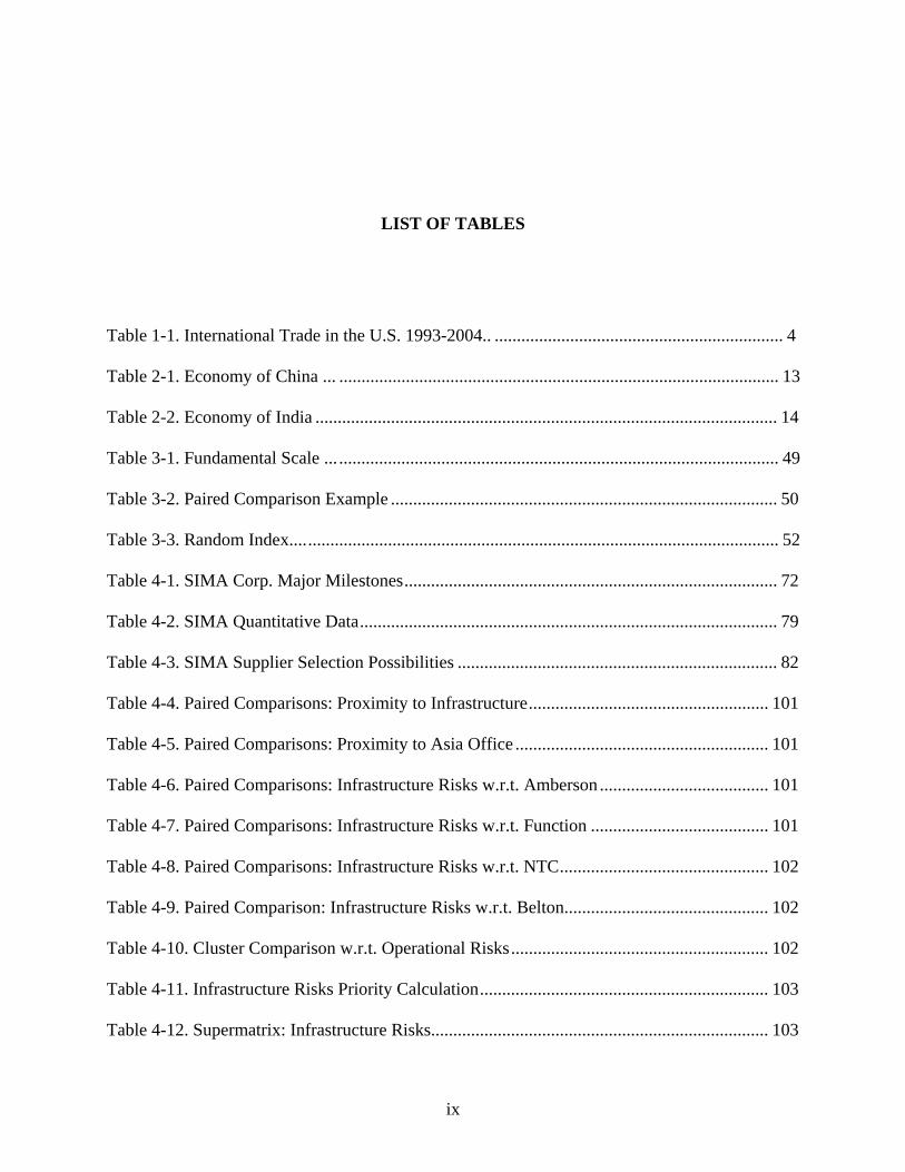
LIST OF TABLES
Table 1-1. International Trade in the U.S. 1993-2004.. ................................................................. 4
Table 2-1. Economy of China ... ................................................................................................... 13
Table 2-2. Economy of India ........................................................................................................ 14
Table 3-1. Fundamental Scale ... ................................................................................................... 49
Table 3-2. Paired Comparison Example ....................................................................................... 50
Table 3-3. Random Index.............................................................................................................. 52
Table 4-1. SIMA Corp. Major Milestones.................................................................................... 72
Table 4-2. SIMA Quantitative Data.............................................................................................. 79
Table 4-3. SIMA Supplier Selection Possibilities ........................................................................ 82
Table 4-4. Paired Comparisons: Proximity to Infrastructure...................................................... 101
Table 4-5. Paired Comparisons: Proximity to Asia Office ......................................................... 101
Table 4-6. Paired Comparisons: Infrastructure Risks w.r.t. Amberson ...................................... 101
Table 4-7. Paired Comparisons: Infrastructure Risks w.r.t. Function ........................................ 101
Table 4-8. Paired Comparisons: Infrastructure Risks w.r.t. NTC............................................... 102
Table 4-9. Paired Comparison: Infrastructure Risks w.r.t. Belton.............................................. 102
Table 4-10. Cluster Comparison w.r.t. Operational Risks.......................................................... 102
Table 4-11. Infrastructure Risks Priority Calculation................................................................. 103
Table 4-12. Supermatrix: Infrastructure Risks............................................................................ 103
x
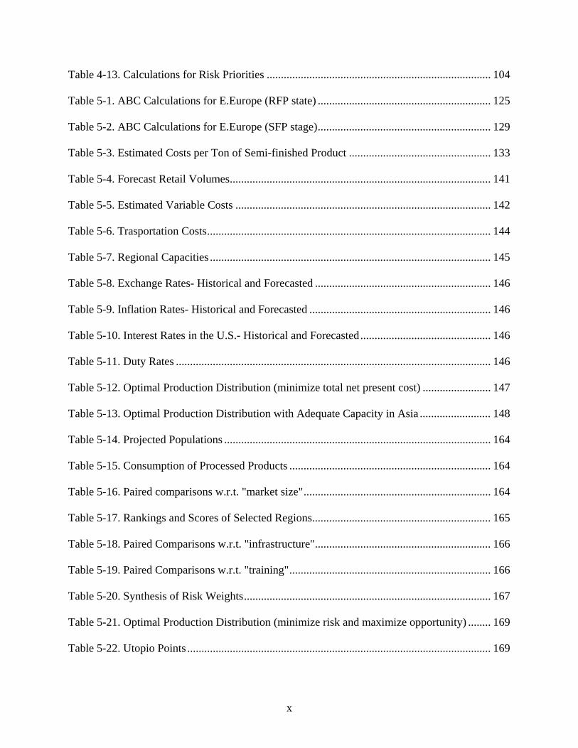
Table 4-13. Calculations for Risk Priorities ............................................................................... 104
Table 5-1. ABC Calculations for E.Europe (RFP state) ............................................................. 125
Table 5-2. ABC Calculations for E.Europe (SFP stage)............................................................. 129
Table 5-3. Estimated Costs per Ton of Semi-finished Product .................................................. 133
Table 5-4. Forecast Retail Volumes............................................................................................ 141
Table 5-5. Estimated Variable Costs .......................................................................................... 142
Table 5-6. Trasportation Costs.................................................................................................... 144
Table 5-7. Regional Capacities ................................................................................................... 145
Table 5-8. Exchange Rates- Historical and Forecasted .............................................................. 146
Table 5-9. Inflation Rates- Historical and Forecasted ................................................................ 146
Table 5-10. Interest Rates in the U.S.- Historical and Forecasted.............................................. 146
Table 5-11. Duty Rates ............................................................................................................... 146
Table 5-12. Optimal Production Distribution (minimize total net present cost) ........................ 147
Table 5-13. Optimal Production Distribution with Adequate Capacity in Asia ......................... 148
Table 5-14. Projected Populations .............................................................................................. 164
Table 5-15. Consumption of Processed Products ....................................................................... 164
Table 5-16. Paired comparisons w.r.t. "market size".................................................................. 164
Table 5-17. Rankings and Scores of Selected Regions............................................................... 165
Table 5-18. Paired Comparisons w.r.t. "infrastructure".............................................................. 166
Table 5-19. Paired Comparisons w.r.t. "training"....................................................................... 166
Table 5-20. Synthesis of Risk Weights....................................................................................... 167
Table 5-21. Optimal Production Distribution (minimize risk and maximize opportunity) ........ 169
Table 5-22. Utopio Points ........................................................................................................... 169

xi
Table 5-23. Pareto Optimal Points- XYZ ................................................................................... 171
xii
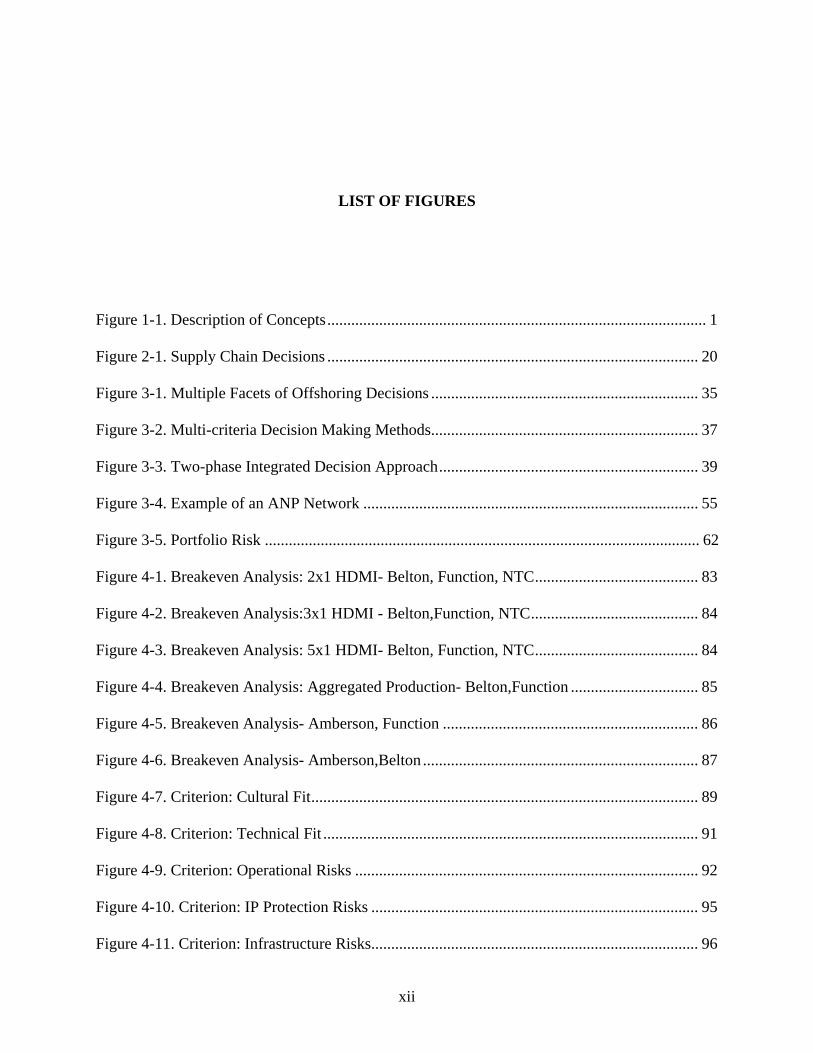
LIST OF FIGURES
Figure 1-1. Description of Concepts............................................................................................... 1
Figure 2-1. Supply Chain Decisions ............................................................................................. 20
Figure 3-1. Multiple Facets of Offshoring Decisions ................................................................... 35
Figure 3-2. Multi-criteria Decision Making Methods................................................................... 37
Figure 3-3. Two-phase Integrated Decision Approach................................................................. 39
Figure 3-4. Example of an ANP Network .................................................................................... 55
Figure 3-5. Portfolio Risk ............................................................................................................. 62
Figure 4-1. Breakeven Analysis: 2x1 HDMI- Belton, Function, NTC......................................... 83
Figure 4-2. Breakeven Analysis:3x1 HDMI - Belton,Function, NTC.......................................... 84
Figure 4-3. Breakeven Analysis: 5x1 HDMI- Belton, Function, NTC......................................... 84
Figure 4-4. Breakeven Analysis: Aggregated Production- Belton,Function ................................ 85
Figure 4-5. Breakeven Analysis- Amberson, Function ................................................................ 86
Figure 4-6. Breakeven Analysis- Amberson,Belton ..................................................................... 87
Figure 4-7. Criterion: Cultural Fit................................................................................................. 89
Figure 4-8. Criterion: Technical Fit .............................................................................................. 91
Figure 4-9. Criterion: Operational Risks ...................................................................................... 92
Figure 4-10. Criterion: IP Protection Risks .................................................................................. 95
Figure 4-11. Criterion: Infrastructure Risks.................................................................................. 96
xiii
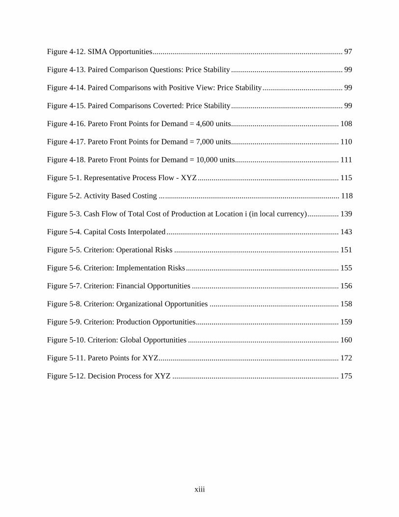
Figure 4-12. SIMA Opportunities................................................................................................. 97
Figure 4-13. Paired Comparison Questions: Price Stability ......................................................... 99
Figure 4-14. Paired Comparisons with Positive View: Price Stability......................................... 99
Figure 4-15. Paired Comparisons Coverted: Price Stability......................................................... 99
Figure 4-16. Pareto Front Points for Demand = 4,600 units....................................................... 108
Figure 4-17. Pareto Front Points for Demand = 7,000 units....................................................... 110
Figure 4-18. Pareto Front Points for Demand = 10,000 units..................................................... 111
Figure 5-1. Representative Process Flow - XYZ........................................................................ 115
Figure 5-2. Activity Based Costing ............................................................................................ 118
Figure 5-3. Cash Flow of Total Cost of Production at Location i (in local currency)................ 139
Figure 5-4. Capital Costs Interpolated ........................................................................................ 143
Figure 5-5. Criterion: Operational Risks .................................................................................... 151
Figure 5-6. Criterion: Implementation Risks .............................................................................. 155
Figure 5-7. Criterion: Financial Opportunities ........................................................................... 156
Figure 5-8. Criterion: Organizational Opportunities .................................................................. 158
Figure 5-9. Criterion: Production Opportunities......................................................................... 159
Figure 5-10. Criterion: Global Opportunities ............................................................................. 160
Figure 5-11. Pareto Points for XYZ............................................................................................ 172
Figure 5-12. Decision Process for XYZ ..................................................................................... 175

xiv
PREFACE
I would like to gratefully acknowledge my dissertation advisor, Dr. Bopaya Bidanda, for his
motivation, inspiration and positive disposition throughout my doctoral study. Additionally, I
would like to extend my sincere gratitude to Dr. Larry J. Shuman who provided me invaluable
advice and generous support. Thank you for believing in me, investing in me and giving
continuous support for my professional and personal development.
Many thanks to my committee members, Dr. Brady Hunsaker, Dr. Ravi Madhavan and
Dr. Kim LaScola Needy for adding value with their expertise and experience. I very much
appreciate suggestions, advice and the insights you brought into this research.
I would like to thank all of the Industrial Engineering faculty members for creating a
spirit of cooperation. Thank you for your commitment to research and education. Special thanks
to Dr. Andrew Schaefer and Dr. Alex Wang for their helpful directions and advice, particularly
in the first years of my study. To my friends from Benedum Hall 10th floor, 5th floor, EGSO and
GPSA. You brought excitement and joy to my life. I wish you all the best in the years to come.
I am grateful to Murat for sharing the best and worst moments of my doctoral dissertation
journey. This dissertation would not be complete without his constant encouragement. Finally, I
would like to dedicate this work to my parents, Nebahat and Emin Arisoy, who have given me
their endless love, support, understanding and everything else that I could ever wish for.

1
1.0 INTRODUCTION
Outsourcing is the transfer of internal functions to an outside corporation whereas “offshore”
outsourcing is the transfer of these functions to overseas locations. A.T. Kearney [1] defines the
relationship between outsourcing and offshoring by classifying the operational transfer into four
parts. The concept of “supply chain and network” in this research is incorporated into this
classification scheme as shown in Figure 1-1.
Captive OffshoringOutsourcing
&Offshoring
Within Company Outside Supplier
Overseas
In DomesticMarket
Domestic Insourcing
Domestic Outsourcing
Global supply chain Global supply network
(local) Supply chain (local) Supply network
Figure 1-1. Description of Concepts
Domestic insourcing and outsourcing happen when the market demand exceeds the
capacity of production (or services) and the company seeks support from either outside suppliers
or inside parties without going outside of the domestic market. These are common practices to
2
enlarge the size of the business temporarily or permanently. On the other hand, a company may
want to broaden its operations by expanding outside of the local region. Typically in these cases
multi-national companies grow globally by investments in different countries. This is called
“captive offshoring.” Instead of making investments, an organization may be willing to go
offshore (perhaps without expanding the market) by contractual agreements with an outside
supplier. By doing so, the risks involved in captive offshoring is mitigated, while some of the
benefits such as lower cost production are accrued. This case is called “offshore outsourcing”
where in many instances the corporations can gain the advantages of international business while
protecting itself from the complications. The term “offshoring” encompasses a company’s
strategic action of going offshore either by outsourcing based on an agreement with a third party
or by investing in an overseas region.
If the operations are performed in-house then the coordination of manufacturing, service
and transportation operations are executed within a chain structure and information flow is
unidirectional against the flow of material. Such a structure is common in a majority of
businesses and it is called a “supply chain.” On the other hand, if the operations are performed
with the participation of outside suppliers, the information and material flows are multi-
directional and their directions may or may not be opposite to each other. Rather than being a
chain, this structure is a “network” of different vendors. Depending on the location of the
operations, the supply chain (or network) is distinguished as global or domestic. This research
focuses specifically on global supply chains and networks with outsourcing and captive
offshoring, which combined is called “offshoring.”
Globalization and offshoring are complementary subjects commonly debated on many
levels. The reality is that globalization is occurring as a result of scientific and technological
3
advancements and its growth likely will escalate. As businesses continue their global expansion
the option of offshoring has also increased as a viable alternative. During this process
organizations encounter decisions concerning the selection of manufacturing and service
locations and the distribution of these manufacturing and service operations. Such strategic
decisions are often assessed from a quantitative point of view where the analyses mostly involve
financial elements. However there are many other factors, including risks and intangible
opportunity variables, which need to be considered with a structured approach for selecting
destination locations and distributions of operations. The purpose of this research is to present a
thorough analysis of offshoring practices and consequently, provide an integrated decision model
that can handle the complexities and multidimensionality of strategic selection of site location
and distribution in order to better optimize global supply chains and networks.
This study first discusses the globalization trend in the world and examines the factors
that lead to the growth of offshoring and the intended and unintended economic and social
consequences in the developed and developing worlds. After a brief discussion, the study focuses
on corporate decisions in going offshore which is followed by the evolution of the supply chain
structure towards a global supply network structure. The literature on corporate decision
making, decision modeling, supply chain management and supplier selection models is
elucidated. Later, the study presents the motivation, development, practice and results of an
integrated decision model that is specifically and extensively built to support offshoring
decisions, including the decision to stay in-house or to go offshore and the decision on where to
locate and how to distribute operations across the world.
4
1.1 MOTIVATION
Globalization is a term that encompasses the increases in the world trade as well as the
borderless worldwide interdependencies within a framework of political and social relationships.
The integration of the global economy through trade has given rise to the interconnectedness of
international economies and politics. Decisions and activities in one part of the world can no
longer remain local; their effects ripple through the societies and economies of multiple
communities in various parts of the world.
The inter-connectedness of national economies, the rapid ascent of countries such as
China and India on the global manufacturing scene, and the pro-active role of the World Trade
Organization, regional alliances, including the European Union, NAFTA and the more fledging
Mercosur (southern Latin America) have all been factors in synergizing this movement towards
Thomas Friedman’s “flat world.”[2] However, the biggest factor has been the high speed
communication links that have arisen over the past ten years which have enabled many high-end,
technical tasks to be performed almost anywhere on the planet.
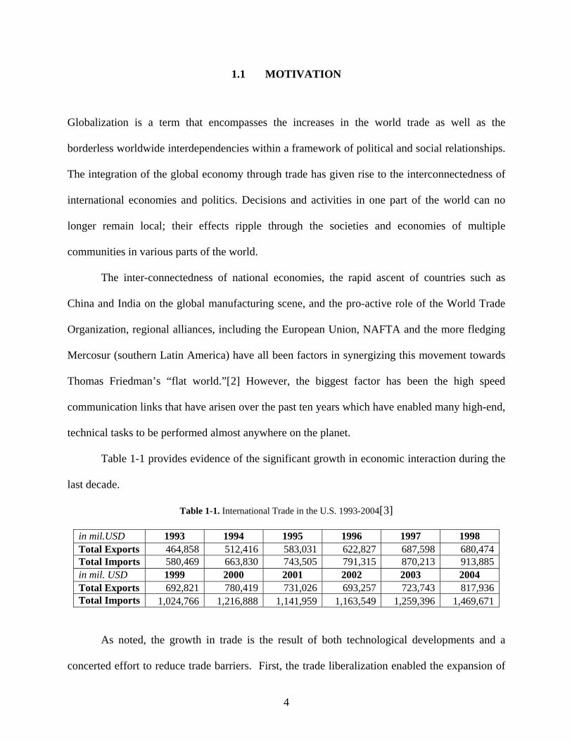
Table 1-1 provides evidence of the significant growth in economic interaction during the
last decade.
Table 1-1. International Trade in the U.S. 1993-2004[3]
in mil.USD 1993 1994 1995 1996 1997 1998 Total Exports 464,858 512,416 583,031 622,827 687,598 680,474 Total Imports 580,469 663,830 743,505 791,315 870,213 913,885 in mil. USD 1999 2000 2001 2002 2003 2004 Total Exports 692,821 780,419 731,026 693,257 723,743 817,936 Total Imports 1,024,766 1,216,888 1,141,959 1,163,549 1,259,396 1,469,671
As noted, the growth in trade is the result of both technological developments and a
concerted effort to reduce trade barriers. First, the trade liberalization enabled the expansion of

5
international relationships. Since 1947, when the General Agreement on Tariffs and Trade
(GATT) was created, the world trading system has benefited from eight rounds of multilateral
trade liberalization, as well as from unilateral and regional liberalization. The last of these eight
rounds (the so-called “Uruguay Round” completed in 1994) led to the establishment of the
World Trade Organization to help administer the growing body of multilateral trade agreements
[4]. Newer organizations such as the European Union and the Mercosur have helped to
accelerate the growth of today’s inter-connected economy (although both the EU and Mercosur
have recently suffered major setbacks in terms of their constitution and the failure to reach a
broader, western hemispheric agreement respectively).
With this trade liberalization in recent years, there have been continuous improvements in
communication and transportation technologies. These two factors have facilitated easy access
to distant locations, especially in large, urban areas around the world. The evolutions in the
Internet and the World Wide Web has had an enormous effect on the communication technology
and the current advances such as wireless networks and quantum computers promise
inconceivable progress for future communications systems.
As a consequence, national boundaries are becoming less important to the large,
multinational corporations who now operate on a global scale. Indeed, as boundaries have
become permeable due to the technological explosion in global communications and low cost
travel, these companies have become transnational, owing allegiance, or even headquarters to no
particular country. This has led to the creation of new markets, new customers, and even a “new
manufacturing order.” Globalization has also spurred competition among companies on an
international scale, especially in the highly developed countries.
6
One result of globalization is the rapid growth of offshore outsourcing or offshoring, i.e.,
the outsourcing of functions and jobs to offshore locations. In the U.S. offshoring has progressed
to the point where it affects everyday lives, from the cars we drive (of which a large portion of
the work and components are outsourced) to computers (which are typically manufactured
offshore and shipped back to the United States) and to electronic diagnostics (where calls are
answered overseas). This phenomenon has implications on our lives and on the jobs that
engineers and scientists will assume both now and in the future. Further, it is something that all
highly developed and even some lesser developed countries must face.
The rapid development of communications systems combined with a competitive need to
find lower cost alternatives without sacrificing quality or performance has resulted in
corporations that operate on a global scale. Rather than this being a new phenomenon, it is part
of a long-term trend that in the U.S. started in the 1970s with manufacturing. Over the past
thirty-plus years an increasing number of U.S. manufacturing jobs, as well as similar jobs in
other highly developed countries, have migrated to countries with substantially lower labor costs.
While these were initially low-end, low-skilled jobs, it is the current movement of high-end,
highly-skilled work that is creating concern within U.S. government, industry and educational
circles. Today the Internet and high-speed data networks enable knowledge tasks to be done
practically anywhere in the world, potentially allowing companies in the developed world to
achieve cost savings or simply to stay competitive enough to remain in business by shifting work
offshore [5]. In addition to the labor cost advantages, the use of English as the medium of
education in such East Asian countries as India and the Philippines has also helped to attract an
increasing amount of outsourced work from the U.S. as well as from European countries and
Japan, Taiwan and Korea. This is especially true as English becomes the primary language of
7
international business [6]. As a result, an increasing movement of work to low-cost countries
continues to appear in certain industries across the developed world.
Due to its significant impact on the economies of both the developing and developed
worlds, offshoring has been subject to many controversial discussions. Although the offshoring
trend drew some attention when blue-collar workers began losing jobs, as U.S. unemployment
rates rose after 2000 and high tech jobs started moving offshore, the effects on the economy of
the current globalization phase is now being questioned. As a result, a large shift towards low-
cost countries has appeared in certain industries at an increasing rate. In fact, offshoring in the
areas of information technology (IT) and business process operations (BPO) has become an
accepted practice [7]. In a frequently cited 2005 report, Forrester Research predicted that 3.3
million U.S. service jobs would be relocated abroad in the next 10 years. Further, McKinsey &
Co. reported that the U.S., Europe and Japan combined are losing 600,000 service and
manufacturing jobs a year [8]. According to Gartner Inc. in another widely cited report, this
trend is likely to continue so that by 2010 one of every four high technology jobs in developed
nations will be outsourced to emerging markets in India, China and elsewhere6. Farrell of
McKinsey and Company has estimated that engineering is the most vulnerable of the professions
relative to offshoring with up to 52% of the jobs at risk 7.
For some people, offshoring is a globalization effort that creates opportunities for future
innovations, contributing to the world economy. For others, it has a destructive effect on local
economies, increasing unemployment rates and weakening the industrial power of the offshoring
country. Above all, offshoring is a result of blending effects coming from globalization and
market competition which actually trigger one another. On one side, world cultures unify
through the rise of communication technologies (a part of globalization) leading to enormous
8
expansion in the consumer and production markets beyond the boundaries of the developed
world. On the other side, political and economic developments, such as privatization of public-
sector organizations and free trade agreements establish a liberated setting for corporations to do
business globally. At the same time, the development of manufacturing processes and
technological enhancements cause a reduction in product life cycles. As a result, both the supply
and demand for low price, high quality and largely customized products (and services) have
increased dramatically. With the growing market competition, big box retailers such as Wal-Mart
and Home Depot gain power over manufacturers. By means of this power shift, retailers have
more incentive for tougher negotiations [9] which leads to an inconceivable chase for low cost
and high quality production and services.
In conclusion, offshoring is not a simple search for lower cost alternatives. It is a
consequence of several intertwined factors that cannot be simply avoided. Companies now go
offshore not simply because of low labor costs. The availability of highly educated young
workers, government subsidies, tax reduction and infrastructural improvement in developing
countries are also attractive for the corporations seeking a competitive edge in the global market.
However, offshoring is not always the best or even the only option for corporations in many
industries. In spite of the immense market competition, in many cases it is more advantageous to
stay in-house for several reasons. The decision as to whether or not to go offshore and where to
go is a complex one. The goal of this research is to investigate the factors that should be
considering in making offshoring decisions and to develop an integrated model that can be
utilized to make the decisions of where (in-house vs. overseas country) and in what proportions
to keep/transfer manufacturing and service operations.

9
1.2 PROBLEM STATEMENT
Today, offshoring stands out as an attractive option for a growing number of companies to
reduce costs of their operational activities by either engaging in direct investment or having
strategic alliances in low-labor-rate countries. From a financial point of view, companies also
anticipate a remarkable reduction in their capital requirements by such moves.
Offshoring ranges from short-term term contracts to long term investments in developing
countries. The decisions of whether or not to go offshore and where and how much
production/service to transfer are important and challenging strategic decisions for corporations.
In many cases, organizational strategies are driven by the economic environment and the market
conditions and for some companies offshoring decisions may be determined by an inevitable
effort to gain competitiveness in the market by lowering the prices and concentrating on the core
competences. However, offshoring does not always lead to greater market share and business
success because there is a much higher complexity in the process. There are numerous
challenges during the implementation, operation and later on supervision of the offshore
processes. According to a Deloitte study [10] 64% of participants brought offshore services back
in-house to regain control and companies recognize the need for improvement in decision-
making.
Global supply networks with offshoring are inherently complex not only because of the
existence of multiple parties and geographical locations, but also because of the
multidimensionality of factors in it. In order to achieve success, corporations need to start by
taking the decision about whether or not to go offshore, where to go offshore and in to what
extend to transfer or keep operations. These decisions involve quantitative and qualitative factors
as well as different expert views. They are sophisticated strategic decisions that need to be
10
analyzed in a comprehensive system. There are various tools such as mathematical modeling
which is a well-established tool to solve decision problems with purely numerical values in
various levels of complexities. In cases where there are many intangible factors, multi-criteria
decision making methods are appropriate to make rational decisions.
In many cases the decisions of going offshore and offshore supplier selection are largely
based on cost analyses where the decision alternatives are evaluated solely on a monetary basis.
The final decision is then often taken by management by considering the intangible factors and
making an approximately good decision based on the results of the cost analysis and intuition.
Although this is the common practice, it may not be the best one. Offshoring has a strategic
importance and affects the performance, profitability and the existence of a corporation. Once an
offshoring decision is made and implemented, it cannot be reversed easily. A small shift from the
optimal decision can have disastrous effects on the competitiveness of the company. Therefore,
it needs preciseness and immense analytical evaluation in a disciplined and structured framework
that can integrate all of the factors in a decision process to generate the best strategic actions.
The offshoring decisions considered in this research are: (1) Whether (or not) to go
offshore, (2) Where to locate operations (selecting suppliers or regions), and (3) How much
production/service to transfer offshore or to keep in-house
This research intends to analyze the nature of offshore outsourcing decisions and develop
a systematic approach by utilizing both mathematical and multi-criteria modeling specifically for
these problems. The objective is to build an integrated decision model that can handle the
multidimensionality of the offshoring decisions involving location selection and distribution of
production and services in global supply networks. A detailed and structured framework of
tangible and intangible factors that should go into such decisions is provided.
11
2.0 LITERATURE REVIEW
The topics of interests in this study can be classified into three areas: offshoring, strategic supply
chain decisions including supplier selection and decision modeling.
There is an extensive literature that discusses the progress, practice and effects of
offshoring. These discussions examine the offshoring phenomenon from different perspectives
and provide background material on the management and decision making process of business
practices that are considered for transferring offshore. They are valuable sources in identifying
the fundamental variables, factors and perceptions that should go into a composite decision
model.
Offshoring is essentially a strategic supply chain decision that includes selection of
suppliers (or regions for investment) and assignment of production and service jobs to those
suppliers (or to the regions). The supply chain management literature presents a large collection
of methods and applications for selecting suppliers, locating businesses, distributing products
and services and managing the relationships in the supply chain. For this reason, the supply chain
management literature provides an invaluable insight on methodologies that can also be utilized
for offshoring decisions.
Decision modeling literature embraces all aspects of decision making (including supply
chain and other business decisions). The application areas and tools for analysis are numerous.
These tools draw from a wide variety of disciplines such as operations research, probability and
12
statistics, economics and psychology. The literature on decision modeling is important in
identifying the most appropriate modeling tools for offshoring decisions in terms of applicability,
ease of use, exhaustiveness and preciseness.
In essence, this study is at the intersection of research on offshoring, supply chain
management and decision modeling. The following literature survey will first present the
evolution of globalization, its consequences on businesses and the concept of offshoring. Then,
a review of supply chain management problems and decision models for strategic decisions in
local and global supply chains will be presented. The last section will provide a detailed
discussion of quantitative and qualitative decision modeling methods that are selected for
developing an integrated approach for offshoring decisions.
2.1 OFFSHORING
The majority of companies operating in the nineteenth and twentieth centuries were vertically
integrated organization that controlled every level of the business including procurement,
production and services. Later, as organizations became horizontal, they spread to multiple
locations in the world, some investing internationally and some procuring globally. The word
“offshoring” and “offshore outsourcing” arose when large parts of organizations such as
manufacturing began to be transferred to low labor rate countries overseas. Although the
phenomenon existed for decades, offshore outsourcing was first identified as a business strategy
in 1989 [11] after Eastman Kodak’s decision to outsource its information technology (IT)
operations. While many businesses were becoming familiar with the idea of offshoring, its
visibility was enhanced with the growth in the number of call centers located in India and rapid
13
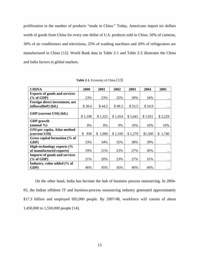
proliferation in the number of products “made in China.” Today, Americans import six dollars
worth of goods from China for every one dollar of U.S. products sold in China. 50% of cameras,
30% of air conditioners and televisions, 25% of washing machines and 20% of refrigerators are
manufactured in China [12]. World Bank data in Table 2-1 and Table 2-2 illustrates the China
and India factors in global markets.
Table 2-1. Economy of China [13]
CHINA 2000 2001 2002 2003 2004 2005 Exports of goods and services (% of GDP) 23% 23% 25% 30% 34% ..Foreign direct investment, net inflows(BoP) (bil.) $ 38.4 $ 44.2 $ 49.3 $ 53.5 $ 54.9 ..
GDP (current US$) (bil.) $ 1,198 $ 1,325 $ 1,454 $ 1,641 $ 1,931 $ 2,229
GDP growth (annual %) 8% 8% 9% 10% 10% 10%GNI per capita, Atlas method (current US$) $ 930 $ 1,000 $ 1,100 $ 1,270 $1,500 $ 1,740 Gross capital formation (% of GDP) 33% 34% 35% 38% 39% ..High-technology exports (% of manufactured exports) 19% 21% 23% 27% 30% ..Imports of goods and services (% of GDP) 21% 20% 23% 27% 31% ..Industry, value added (% of GDP) 46% 45% 45% 46% 46% ..
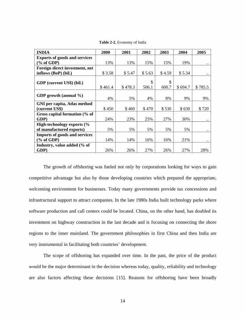
On the other hand, India has become the hub of business process outsourcing. In 2004-
05, the Indian offshore IT and business-process outsourcing industry generated approximately
$17.3 billion and employed 695,000 people. By 2007-08, workforce will consist of about
1,450,000 to 1,550,000 people [14].
14
Table 2-2. Economy of India
INDIA 2000 2001 2002 2003 2004 2005 Exports of goods and services (% of GDP) 13% 13% 15% 15% 19% ..Foreign direct investment, net inflows (BoP) (bil.) $ 3.58 $ 5.47 $ 5.63 $ 4.59 $ 5.34 ..
GDP (current US$) (bil.) $ 461.4 $ 478.3
$ 506.1
$ 600.7 $ 694.7 $ 785.5
GDP growth (annual %) 4% 5% 4% 8% 9% 9%
GNI per capita, Atlas method (current US$) $ 450 $ 460 $ 470 $ 530 $ 630 $ 720Gross capital formation (% of GDP) 24% 23% 25% 27% 30% ..High-technology exports (% of manufactured exports) 5% 5% 5% 5% 5% ..Imports of goods and services (% of GDP) 14% 14% 16% 16% 21% ..Industry, value added (% of GDP) 26% 26% 27% 26% 27% 28%
The growth of offshoring was fueled not only by corporations looking for ways to gain
competitive advantage but also by those developing countries which prepared the appropriate,
welcoming environment for businesses. Today many governments provide tax concessions and
infrastructural support to attract companies. In the late 1980s India built technology parks where
software production and call centers could be located. China, on the other hand, has doubled its
investment on highway construction in the last decade and is focusing on connecting the shore
regions to the inner mainland. The government philosophies in first China and then India are
very instrumental in facilitating both countries’ development.
The scope of offshoring has expanded over time. In the past, the price of the product
would be the major determinant in the decision whereas today, quality, reliability and technology
are also factors affecting these decisions [15]. Reasons for offshoring have been broadly
15
investigated by academicians and industrial experts. According to Deavers [16], four
fundamental changes in the global market lead to the increase of offshoring. These are:
1- Rapid technological change
2- Increased risk and the search for flexibility
3- Greater emphasis on core competencies
4- Globalization
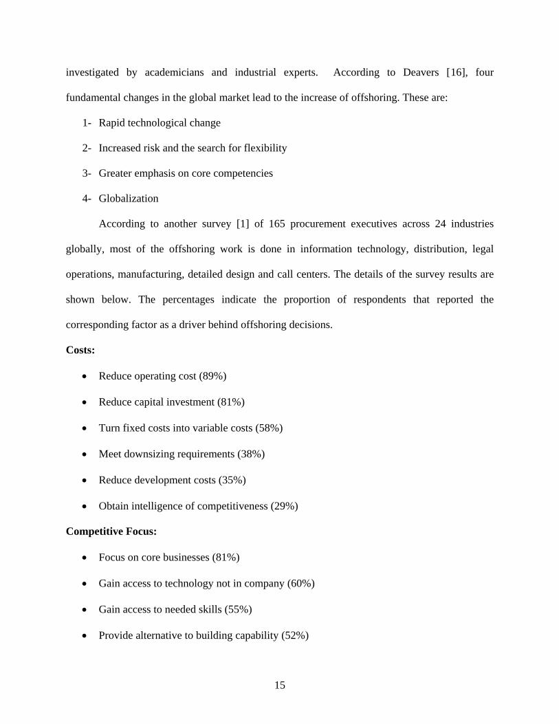
According to another survey [1] of 165 procurement executives across 24 industries
globally, most of the offshoring work is done in information technology, distribution, legal
operations, manufacturing, detailed design and call centers. The details of the survey results are
shown below. The percentages indicate the proportion of respondents that reported the
corresponding factor as a driver behind offshoring decisions.
Costs:
• Reduce operating cost (89%)
• Reduce capital investment (81%)
• Turn fixed costs into variable costs (58%)
• Meet downsizing requirements (38%)
• Reduce development costs (35%)
• Obtain intelligence of competitiveness (29%)
Competitive Focus:
• Focus on core businesses (81%)
• Gain access to technology not in company (60%)
• Gain access to needed skills (55%)
• Provide alternative to building capability (52%)
16
• Create additional capacity (42%)
• Provide backup capabilities (34%)
• Align with policy/philosophy/culture (18%)
Revenue:
• Increase flexibility and responsiveness (60%)
• Increase speed to market (46%)
• Improve quality (42%)
• Reduce customer response time (40%)
• Grow revenue (38%)
• Gain access to markets (22%)
The immediate results can be seen as cost savings and asset reductions in the short term.
Program flexibility, enhanced attention to critical customer service and lower turnover rates are
also some of the direct consequences. Furthermore, several companies pursue international talent
and opportunities for bigger foreign markets through economic investment [17]. In the long
term, good decisions in offshoring practices give competitive advantage by improving
productivity and ensuring concentration on core competences.
On the other hand, the results of offshoring are not always satisfactory. There are
numerous examples of offshoring projects that failed due to unexpected complications.
According to a DiamondCluster survey of 210 companies offshoring IT services, recently there
has been significant decline in offshoring satisfaction levels [18]. The same research also reports
that the number of IT offshoring contracts terminated abnormally has doubled from 2004 to
2005; 36% of survey participants cited poor provider performance as the primary reason whereas
17
change in strategic direction, transfer of function in-house and dissatisfaction in cost savings
were cited by 16%, 11% and 7% of participants, respectively.
Offshoring failures can be broadly categorized into two reasons: financial problems and
operational problems. Financial problems arise when the anticipated cost savings cannot be
realized as a result of wrong assumptions. When production and service costs in a developing
country (such as China and India) are compared to the costs in the U.S., the difference may be
deceptively perceived as cost savings. Yet, the cost differences cannot be fully incurred as
savings due to the hidden costs behind the offshore process. For instance, with any outsourced
service, the expense of selecting a service provider can cost from 0.2% to 2% in addition to the
annual cost of the contract [19]. There are also costs involved in managing the distributed
operations which include travel costs, legal documentation fees and communication expenses.
Managers often need to travel periodically to manage the operations that are miles away. Overall,
when hidden costs are factored in, the cost savings may not be as large as expected.
In addition to the financial problems, offshore failures may appear due to other factors.
Cultural differences and communication difficulties are rapidly becoming challenges that are not
easy to overcome. Even though cultural differences are getting less severe with the development
of media channels and the Internet, perceptions are still not the same. For instance in an Asian
company, a message may not be appreciated without going through different levels of hierarchy
within the organization in contrast to the U.S. Both the practice and the governance of offshoring
needs effort, money and flexibility. Exogenous factors such as political stability, infrastructure
and economical conditions in the country affect the performance of operations. Profits are
directly altered by currency fluctuations and inflation rates. Even if the offshore manufacturer or
service provider meets the technical, quality and capacity criteria, the environmental factors
18
within the region may limit the operations. For this reason a company needs to choose the
country based on not only the cost levels but also on the macro-economic and political
conditions.
Although some factors leading to failure can be eliminated by proper governance and
management, it should be noted that offshoring is not always a good strategy. Among the
primary reasons that a company chooses not to outsource are concerns over loss of control,
intellectual property protection and willingness to keep core activities inside. Company policy
and philosophy are also revealed as a rationale for staying in-house [20]. Moreover,
decentralization of operations globally complicates the supply chain. The fact is that product
flows in global supply networks are slower with a loss in flexibility. For example some
organizations within the fashion industry like American Apparel choose to stay in the U.S. to
maintain their competitiveness in fast product launches.
In summary, offshoring is a complex decision that may lead to both gain and loss of
competitive advantage. It is a strategic decision involving the design and control of an
organization’s global supply network. Its importance and complexity necessitates structured
guidelines for evaluating the short and long term consequences upon the business. The
offshoring decision is a strategic problem in supply chain management, which is commonly
encountered by today’s large corporations.
2.2 DECISION MODELS IN SUPPLY CHAIN MANAGEMENT
Decision models are critical in the evaluation of data to gain greater understanding of the
problem at hand. Decision analyses and models have been of interest to scholars from several
19
research areas, including management science, operations research, mathematics and
psychology. In the last decade, researchers have developed decision models that facilitate
strategic configuration of supply chains. A large part of this research concentrates on strategic
decisions involving facilities, transportation and distribution within local geographic regions.
The complexity of these decision problems escalates as the businesses expand globally and the
supply chains become global supply networks with the inclusion of international partners and
offshoring.
Literature in the supply chain management area is vast and can be classified into four
major decision areas: location, production, distribution and inventory. This study focuses mainly
on strategic location and distribution decisions. The next section presents a review of the
literature with a concentration of location/supplier selection models. As companies grow
internationally, the research on supply chain management expanded to embrace the complexities
in global operations and the decisions specific to offshoring. The latter section will review the
models that are specifically developed for complex supply networks operating in multiple
locations.
2.2.1 Strategic Supply Chain Models: Supplier Selection
Supply chain management decisions are conceived in three levels: strategic, tactical and
operational. Figure 2-1 gives a schematic description of decisions in supply chains. Strategic
decisions are long range and involve designing the supply chain, selecting the size and
geographic locations for manufacturing, service and distribution operations and implementing
control systems. Tactical decisions are medium term and determine the monthly (or weekly)
production schedules, distribution and transportation planning and materials requirements
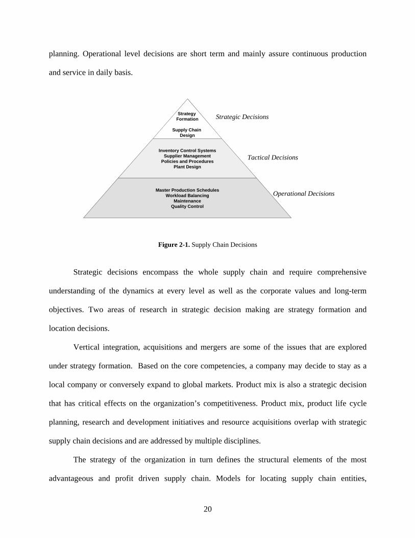
20
planning. Operational level decisions are short term and mainly assure continuous production
and service in daily basis.
Strategy Formation
Supply Chain Design
Inventory Control SystemsSupplier Management
Policies and ProceduresPlant Design
Master Production SchedulesWorkload Balancing
MaintenanceQuality Control
Strategy Formation
Supply Chain Design
Inventory Control SystemsSupplier Management
Policies and ProceduresPlant Design
Master Production SchedulesWorkload Balancing
MaintenanceQuality Control
Strategic Decisions
Tactical Decisions
Operational Decisions
Figure 2-1. Supply Chain Decisions
Strategic decisions encompass the whole supply chain and require comprehensive
understanding of the dynamics at every level as well as the corporate values and long-term
objectives. Two areas of research in strategic decision making are strategy formation and
location decisions.
Vertical integration, acquisitions and mergers are some of the issues that are explored
under strategy formation. Based on the core competencies, a company may decide to stay as a
local company or conversely expand to global markets. Product mix is also a strategic decision
that has critical effects on the organization’s competitiveness. Product mix, product life cycle
planning, research and development initiatives and resource acquisitions overlap with strategic
supply chain decisions and are addressed by multiple disciplines.
The strategy of the organization in turn defines the structural elements of the most
advantageous and profit driven supply chain. Models for locating supply chain entities,
21
determining the capacity of manufacturing and establishing transportation routes are used to
assist strategic supply chain management decisions. This research focuses mainly on decision
models to select locations of suppliers and facilities and determine the distribution of
manufacturing/service products among these locations. These decision models are derived from
different disciplines and their content as well as approach vary depending on the tools used. A
brief summary of the widely-used model types and their applications in location and supplier
selections is given. These models are also analyzed with respect to their appropriateness and
applicability for offshoring decisions.
Mathematical Modeling:
In operations management, the biggest concentration has been on mathematical modeling
of supply chain decisions by using formulations to express elements of the supply chain (i.e.,
product quantities, time, sequence). Location and supplier selection problems are often
formulated as mixed integer programming models by representing the product quantities with
continuous variables and the selections by discrete variables. Geoffrion and Graves [21]
presented the first mixed integer model to find the optimal location of distribution facilities in a
supply chain. The problem is formulated as a multi-commodity capacitated single-period
problem. A solution technique based on Benders Decomposition is developed, implemented and
applied to a real life problem with 17 commodity classes, 14 plants and 45 possible distribution
center sites.
Mixed integer programming (MIP) encompasses decision variables corresponding to both
location selection (binary) and distribution of production/service (continuous). MIP is a reliable
efficient modeling technique for medium size problems and it can support decisions by covering

22
quantitative attributes. It is an appropriate and effective technique to achieve precise, optimal
solutions for offshore supplier and destination selection models. There is a vast literature on MIP
to solve supplier and location selection problems. The MIP methodology and its applications will
be discussed further in the next sections.
Total Cost Models:
Total cost models focus on selecting the supplier which provides products (or services)
with at the least cost over a period of time. Mathematical programming is also used in many of
these models but instead of minimizing only the cost of product, these models minimize the total
cost of procurement by including transportation, invoicing and negotiations. Degraeve and
Roodhooft [22] presented the first total cost model in the context of supplier selection by using
information from management accounting to calculate the total cost of ownership by means of
activity based costing, leading to the selection of the best supplier(s). The authors implemented
the decision model at a large multinational Belgian steel producer and test it for two product
groups. In another publication [23], they compared different supplier selection models and
conclude that mathematical programming combined with activity based costing provide superior
answers.
AHP & ANP:
Analytic Hierarchy Process (AHP) and Analytic Network Process (ANP) are multi-
criteria decision models that fundamentally rely on comparison of entities with respect to criteria
by using a ratio scale. The details of the theory and application of these methods will be
discussed in the next section. These methods have attracted much attention from different areas
23
including supply chain management. There are various applications of AHP and ANP in supplier
and location selection literature. An example is a group decision tool developed by Muralidharan
et al. [24] by integrating the Delphi method and AHP for supplier selection problems.
Confidence intervals of the AHP ratings done by individuals are calculated and depending on the
interquartile range, the ratings are repeated by utilizing the Delphi method. This procedure helps
reduce the effect of individual biases. Even though the AHP and ANP methods may not be as
precise as mathematical modeling in terms of the quantitative decision variables, they provide a
strong tool to quantify intangible values that otherwise are not easily included in a decision
model. It also supports group decision making by integrating perspectives of different
stakeholders.
Multi-objective Programming:
A supplier selection problem involves optimization of multiple objectives which are often
conflicting. Multi-objective programming allows solving multiple objectives by assessing the
tradeoffs between the solutions. More discussion on multi-objective programming can be found
in the next sections. Multi-objective programming is used as a tool in many areas including
supplier selection problems. One of the most recent works combines fuzzy methods with multi-
objective optimization problem. Amid et al. [25] presented a fuzzy multi-objective supplier
selection model in which the objectives are not equally important and have different weights.
The authors applied the model on a numerical example and perform sensitivity analysis. This
model is useful in encompassing different objectives.

24
Multi-attribute Utility:
In economic theory, utility is understood as a numerical representation of a preference
relation; preferences are assumed to satisfy certain conditions of internal consistency, which
ensure that a utility representation exists for preferences and that choosing consistently with
one’s preferences can be represented as the maximization of utility [26]. Utility of a reward is
denoted as a function of that reward (r), and is elicited by asking the decision maker the
indifference point between the preference of r and the preference of a probabilistic combination
of the least and most favorable outcomes. According to utility theory, the decisions are made by
maximizing the utilities of the attributes which affect the decision. For instance if a decision is
solely based on monetary outcomes, the decision maker chooses the alternative which maximizes
the utility of that outcome. If a decision is made based on multiple attributes, the decision
maker’s preference is expressed as a multi-attribute utility function that represents the compound
utility coming from all of the attributes.
Utility theory and multi-attribute utility modeling have been interest to scholars from
different areas, including supply chain management. As an example, Min [27] introduced a
multi-attribute utility approach for international supplier selection problems. The author first
structured the international supplier selection problem into a hierarchy of four levels and then
determined the main attributes such as service performance, quality assurance and
communication. The approach is illustrated with a base-line scenario that involves selecting the
most appropriate foreign supplier that manufactures and sells the components of personal
computers.

25
Conceptual Models:
Conceptual models have been developed in an effort to build a decision and a control
mechanism for corporations. These models are not meant to solve specific decisions in an
analytical framework; rather they are geared towards implementing a business strategy.
The SCOR (Supply Chain Operations Reference) model is a strategic decision making
tool developed by the Supply Chain Council [28]. A process reference model is described as one
that integrates the concepts of business process re-engineering, benchmarking, and process
measurement into a cross-functional framework. THE SCOR model is built in detail to capture
management processes in a supply chain; by using performance metrics the supply chain
performance is monitored and continuously improved. SCOR structurally describes, measures
and evaluates supply chain configurations.
2.2.2 Integrated Models
A more comprehensive evaluation of supply chains requires the integration of performance
factors other than costs. There is a limited amount of research on supplier and location selection
models that utilize multiple methods from different disciplines. As supply chains expand both in
terms of the location dispersion and the complexity of management, the necessity for using
multiple tools increases.
Talluri and Baker [29] proposed a multi-phase mathematical programming approach that
designs an effective supply chain by considering the efficiencies of participating candidates,
capacity and transportation issues. The model incorporated multiple objectives but all of these
objectives are quantitative measures.
26
Ghoudyspour and O’Brien [30] proposed a method that integrates AHP and linear
programming by formulating a linear program with the objective of maximizing the total rating
score of procurement. Each supplier’s score is determined by using an AHP model that includes
quality, cost and service criteria and these scores are multiplied by the amount of procurement
from each associated supplier; their sum is then maximized subject to demand and capacity
constraints. Although the proposed model is an effort to integrate quantitative factors in supplier
selection, the integration is not theorically consistent. The calculation of supplier score involves
the addition of quality, cost and service ratings, however the principal of engineering economic
benefit/cost analysis requires the assessment of incremental differences, rather than a simple
addition. Moreover, the model does not include the fixed costs involved and assumes that the
cost, quality and service values are linearly proportional to the product amount. Such an
assumption is not valid in practical cases where the suppliers usually quote different prices on
different amounts and charge fixed ordering costs.
Instead of finding the best supplier selection, Weber et al. [31] followed a different
approach and illustrate how multi-objective programming and data envelopment analysis can be
used to evaluate the number of suppliers to employ. The authors took into account the fact that
the low cost supplier is not always the one with the best performance. The model finds the non-
inferior set of suppliers whose criteria values are most in line with specified criteria weights.
Although these models have a strong foundation in supply chain design, they lack
complexities that are encountered in global environment. For example political risks and social
opportunities are not taken into account. Recently the research on strategic decisions for supply
chains has broadened to include supply networks that are located internationally. The next
27
section will give an overview of models that are developed specifically for global supplier and
location selection problems with offshoring.
2.2.3 Global Supply Network Models
One effect of globalization is that more organizations are doing business internationally. Today,
supply chains can no longer be defined as series of suppliers that are connected linearly, rather
suppliers have relationships that involve two-way commodity flows with one-to-many
connections. Additionally, these supply networks are located internationally, usually distributed
in different continents. Unlike local supply chains global supply networks include variables that
cannot be controlled by the decision maker. For instance risks associated with macroeconomic
conditions in different regions and cultural as well as social diversity add enormous uncertainty.
Moreover, today’s global variables supply networks mostly embrace offshore practices that
require consideration of multiple both during the decision and process and through the
operations. For this reason, global supply networks are modeled with more sophisticated
formulations to incorporate the complications of various factors. The inclusion of taxes and
duties, fluctuating exchange rates, trade barriers, transfer prices and duty drawbacks is
fundamental for a model to more accurately represent a global supply network problem [32].
Compared to traditional supply chains there is a limited body of literature focusing on the
modeling of global supply networks and offshoring decisions. The number of publications and
researchers interested in the area is increasing rapidly, but still the extent is limited short for the
global supply network problems.
As in the case of traditional supply chains, the decision modeling literature can be
divided into two streams. One stream of literature extensively utilizes operations research
28
techniques to model the decisions and assess the profitability of production (or service)
operations on the basis of quantitative variables. The other stream of literature concentrates on
intangible determinants and evaluates the drivers and consequences of global operations by
examining the business conditions, risk factors, opportunities and other qualitative as well as
quantitative variables.
The mathematical formulation based literature on decision models in global supply
networks mostly includes tools from decision sciences, operations research and economics. A
review of applications was presented by Cohen and Mallik [33] in which the authors discuss the
globalization of supply chains. These models typically include financial parameters and address
global supply network problems to find production quantities, production locations, distribution
routes, etc. The next section provides examples from various disciplines that utilize different
methodologies to model the global supply networks and solve the global supplier and region
selection and production allocation problems.
Arnzten et al. [34] have formulated a global supply chain model (GSCM) that minimizes
a weighted combination of total cost and activity days where the total cost includes production
and inventory costs, taxes, facility fixed charges, production line fixed costs, transportation costs,
fixed costs associated with a particular method of manufacturing, and duty avoidance. This MIP
model is solved for a digital equipment corporation that is in the process of determining plant
charters and allocation of production loads. The model is then utilized to analyze the supply
chain for new products as well as the supply bases for existing commodities. The decision model
is applicable to a multi-stage, multi-product manufacturing environment.
Huchzermeier and Cohen [35] developed a stochastic dynamic programming formulation
for the valuation of global manufacturing options. These options are delineated by distinct time

29
periods that are defined by the available sources of supply, plant capacities, product allocations
to market regions, and open supply linkages within the global supply network. There is a cost
associated with switching between options over the time horizon of the strategic decision. The
model maximizes the global after-tax profits and incorporates option valuation and exchange
rates.
Nagurney et al. [36] developed a framework for the modeling and analysis of global
supply networks. The authors built an extensive mathematical model that includes dynamics of
price and behaviors of supply chain partners. The model maximizes the total profit by deciding
on the amount of product shipments based on the costs as well as the equilibrium prices of
products in different currencies at the various demand markets (countries). It allows for the
analysis and solution of the equilibrium product flows and prices by considering the behavior of
multiple parties (customers, retailers, etc.) in the supply network. The authors apply an iterative
algorithm to compute solutions to several numerical examples.
Grossman and Helpman [37] studied the determinants of outsourcing and model
outsourcing activities as the equilibrium of production and trade between the parties. The authors
presented an economic model of location selection with respect to market conditions, supplies
and demands. The authors first studied how labor supply, country size and technological
investment affect the pattern of outsourcing and location equilibrium. Then they investigated the
role of the contracting environment by incorporating the legal setting of countries. Based on
macroeconomic and product cost data, the authors drew conclusions on how an organization
should proceed in choosing specific locations to transfer activities.
Kouvelis and Munson [38] developed a mixed integer model to represent the cost of
global facility networks by incorporating government subsidies, tariffs and taxations. They
30
presented an MIP formulation that maximizes the net present value of profit subject to demand
and capacity constraints. The model incorporates the time value of money by including the
interest rates on loans and discount rate of after tax cash flows for each country. Based on the
MIP formulation, the authors found the variables which significantly influence the solution and
develop a structural equation by using these variables.
Goetschalckx et al. [39] presented two global logistics system models. The first one is a
non-convex optimization problem that focuses on the transfer prices in a global supply chain
with an objective of maximizing the after tax profit of an international corporation. The second
one focuses on the production and distribution allocation of a single country system when
customers have seasonal demands.
Steenhuis and De Burijn [40] followed a different approach and compare manufacturing
location alternatives in a global supply network by utilizing productivity measures as the basis
for analyzing the international location/industry combination options. GDP values and
dependencies of industries are used to calculate the productivity levels in each country (or
region) and a decision process that can be utilized by both corporations and governments is
suggested.
The other stream of literature concentrates primarily on the qualitative determinants of
global operations such as risk, knowledge bases and market opportunities. Researchers in both
academia and industry have generated various studies that emphasize the value of intangible
attributes in global supplier selection and production allocation decisions.
Bartmess and Cerny [41] stated that capability focused approaches to the facility location
decision in global environment will support a company’s competitive advantage on an enduring
basis. Traditional approaches such as static snap-shot analysis and single functional focus can
31
provide only short-term solutions that will not lead to long-term benefits. Instead, the authors
propose capability focused approaches including non-manufacturing issues and demonstrate the
superiority of these approaches by giving real business examples.
MacCormack et al. [42] examined the impact of qualitative factors on the performance
and efficiency of global supply networks. They called attention to the importance of
incorporating parameters such as exchange rates, tax systems, government regulations and
technological capabilities. The authors presented an overview of the macroeconomic and
business level trends while summarizing the technological advances in production systems and
related trends in management philosophies. After highlighting the insufficiency of cost based
decision models, the authors proposed a new framework for assisting in site location decisions
and a model of the future global manufacturing firm.
The global management consulting firm A.T. Kearney [43] has developed a scheme for
offshore decisions based on the offshore location attractiveness indices of countries. Their report
also highlights the issues that corporations must balance in their strategic offshore decisions.
Countries are evaluated based on corporate surveys, current offshore IT and business process
outsourcing activities, labor skills and availabilities, business environment, infrastructure, culture
adaptability, security of intellectual property, and financial structure.
On the other hand, the Global Outsourcing Report 2005 [44] assesses countries in terms
of two indices: the Global Outsourcing Index (GOI) and the Future Outsourcing Rank (FOR).
According to this report, India and China are the two distinct low-cost labor countries that
emerge as leaders for organizations considering outsourcing. China is mostly known for low cost
manufacturing labor, whereas India has the advantage of an English speaking population and
thus attracts a large amount of Business Process Outsourcing (BPO) and IT contracts.
32
Alternatively, Taiwan and Korea are known as the centers of the semi-conductor industry.
Besides these big players, countries such as Indonesia, Philippines and Malaysia also can
effectively compete for the offshoring business.
Multi-attribute modeling approaches are also exploited in order to integrate intangible
decision variables into supply network decisions. Udo [45] employed the analytic hierarchy
process (AHP) technique to analyze information system outsourcing decisions. The supplier of
choice is selected based on five criteria: strategic importance, stakeholder’s interest, supplier’s
issues, cost of operations and industry environment. The supplier alternatives are assessed by
paired comparisons and the decision is made based on the overall synthesized ranking values
associated with each supplier. In another application, Badri [46] combined AHP with goal
programming for a global facility location allocation problem. The author first defines seven
quantitative goals, including minimizing the total cost and maximizing the environmental
quality. Then, AHP is used to determine weight factors for each goal, and goal programming is
used to solve the aggregate model.
2.2.4 Summary
As more businesses are expanding globally and more processes are outsourced, the need for
detailed global supply network modeling escalates. Supplier selection, determining locations of
suppliers and the allocation of production and services require consideration of quantitative and
qualitative criteria. These decisions often involve many alternatives and conflicting objectives as
well as constraints arising from uncertainties associated with the economy of countries. The
literature includes various applications of supplier and location selections models that utilize
tools like multi-attribute modeling, mathematical modeling, artificial intelligence, expert
33
systems, multivariate statistical analysis and multi-attribute utility models. Some of the models
integrate different tools to incorporate intangible variables, too. However there is not a
systematic approach that:
• Includes all of the quantitative and qualitative criteria involved. There are models which
consider some of these criteria but there is no single model that actually defines the risks
and opportunities and then incorporates these into a decision approach.
• Is designed specifically for global supplier and location selection. In particular, the
offshoring phenomenon is not adequately emphasized as a part of the decision process.
• Uses both continuous and discrete decision variables to represent the supplier and
location selection problem and the problem of allocating products and services.
• Facilitates sensitivity analysis, therefore assists the decision maker in negotiations and
decision changes in case of prospective economical and social variables.
• Encompasses the complexity, interdependency and vastness of criteria in global business
processes and the decisions associated with global practices.
• Deals specifically with the offshoring problems and the decision of whether or not to go
offshore.
This research aims to provide a decision approach that can alleviate these gaps in the
published literature. The next section presents the methodology used in the decision approach
developed in this study.
34
3.0 METHODOLOGY
Offshoring decisions are similar to strategic supply chain decisions involving location selection
and production distribution. The difference is that offshoring decisions are more complex
necessitating an integrated decision making approach that can manage various tangible and
intangible factors. The next section will detail the factors affecting offshoring. Finally, the
methodology for developing an integrated decision making approach is presented.
3.1 PROBLEM CHARACTERISTICS
Although some perceive offshoring as a strategic decision made in response to the inflating cost
competition, in essence it has multiple facets that should be considered during the decision
process. Even though cost is often the primary objective there are many other objectives such as
concentration in core competences. In choosing an offshore supplier and a location a company
wants to minimize the total risk of going offshore while realizing the benefits of it. There also
are several stakeholders who may have conflicting expectations and priorities. For instance, for
shareholders cost reduction is the most important outcome whereas for customers, product and
service quality may be as important as the price. Therefore, the decision needs to be considered

35
not only in terms of different objectives, but also from different perspectives. Figure 3-1 presents
the multiple facets of offshoring decisions in a scheme.
Quantitative V ariables
Objectives
Qualitative V ariables
StakeholdersOffshoring
Decision
Quantitative V ariables
Objectives
Qualitative V ariables
StakeholdersOffshoring
Decision
Figure 3-1. Multiple Facets of Offshoring Decisions
It may be computationally complex but often not very difficult to identify good
offshoring decisions in terms of monetary values. There are well-established mathematical tools
to evaluate the financial factors that can lead to profitable results. On the other hand, financial
factors are only one determinant in the decision space that can make an offshoring process
successful. Offshoring is a long-term strategic action that has risks and benefits that are not
always reflected in a financial statement. Thus, only a decision model that covers all of the
intangible values as well as the monetary objectives can give a reliable offshoring strategy. The
existence of multiple objectives, stakeholders, tangible and intangible values necessitates a
systematic approach that can synthesize strengths of multiple tools.
36
3.2 SOLUTION APPROACH
Operations research tools are commonly used for modeling and optimizing systems with tangible
values. These models are practical and can accurately represent complex systems with several
constraints and variables. For an offshoring decision, cost minimization (or profit maximization)
is a major objective which can be expressed mathematically as a function of production and
service amounts. Transaction costs and other constraints can also be formulated in a
mathematical model. From a cost minimization perspective, mathematical modeling techniques
can give the optimal offshoring decision. Rationale for the selected methodologies are detailed
in the next sections
The cost of operations consists of fixed costs such as asset depreciation (site selection) as
well as variable costs that vary with production and service amount. For this reason, finding the
optimal distribution of products and services in a network of possible alternative suppliers (or
locations) requires inclusion of both discrete and continuous variables in a mathematical model.
Continuous variables represent production and service amounts whereas selection of suppliers is
represented by binary (0-1) variables. Such a problem with a mixture of integer and continuous
variables can ideally be formulated as a mixed-integer programming problem.
Although such a mixed-integer program can find the best supplier and location selection
along with the optimal production and service distributions, it does not embrace the intangible
factors that significantly influence the decisions in offshoring. For example, organizations
operating in a global environment are subject to political risks that exist overseas. Moreover, the
community perspective is a very important issue for global decisions, especially for offshoring
decisions where there are controversial arguments which can affect the welfare of stakeholders.
In order to obtain a comprehensive and reliable decision, the qualitative values associated with
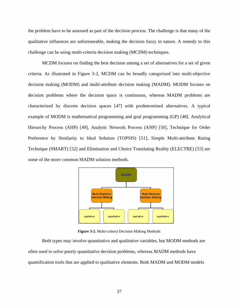
37
the problem have to be assessed as part of the decision process. The challenge is that many of the
qualitative influences are unforeseeable, making the decision fuzzy in nature. A remedy to this
challenge can be using multi-criteria decision making (MCDM) techniques.
MCDM focuses on finding the best decision among a set of alternatives for a set of given
criteria. As illustrated in Figure 3-2, MCDM can be broadly categorized into multi-objective
decision making (MODM) and multi-attribute decision making (MADM). MODM focuses on
decision problems where the decision space is continuous, whereas MADM problems are
characterized by discrete decision spaces [47] with predetermined alternatives. A typical
example of MODM is mathematical programming and goal programming (GP) [48]. Analytical
Hierarchy Process (AHP) [49], Analytic Network Process (ANP) [50], Technique for Order
Preference by Similarity to Ideal Solution (TOPSIS) [51], Simple Multi-attribute Rating
Technique (SMART) [52] and Elimination and Choice Translating Reality (ELECTRE) [53] are
some of the more common MADM solution methods.
Figure 3-2. Multi-criteria Decision Making Methods
Both types may involve quantitative and qualitative variables, but MODM methods are
often used to solve purely quantitative decision problems, whereas MADM methods have
quantification tools that are applied to qualitative elements. Both MADM and MODM models

38
contribute to the decision science literature and have an accepted scientific base. The
applicability of each method depends on the configuration of the specified decision problem.
MADM methods utilize different tools to quantify the intangible values by elucidating
the preferences of decision makers. Utility theory is a widely used tool to derive mathematical
functions based on individuals’ desirability and preferences towards particular actions. However,
in practice obtaining utility functions in such a complex situation with many different attributes
is time consuming, computationally demanding and perhaps not even possible.
Preferences of decision makers can also be elucidated by other tools without expressing
them in terms of mathematical functions. MADM methods such as ELECTRE, TOPSIS, AHP
and ANP can quantify qualitative attributes and find the best selection(s) from a set of outcomes
by eliciting the decision maker’s preference. These methods can be used to evaluate the
intangible factors in a decision method in a much simpler and effective way.
Among these, ANP is the method that can handle complicated decision problems with
multiple stakeholders including dependencies among criteria and alternatives. It can decision
problems in a network structure by means of influence projections. Although the methodology’s
mathematical evaluation may be overwhelming for large problems, its accompanying software
package “Superdecisions [54]” enables assistance and flexibility in its application.
ANP is the generalized version of AHP which is a type of additive weighting method,
developed by Saaty in 70’s. AHP, and later ANP, has been very popular in the decision literature
and has been widely utilized. Both methods are straightforward and easy to use and are
incorporated in software packages that make their applications more convenient. The methods
integrate subjective judgments with numerical data and can monitor the inconsistencies in
subjective judgments.
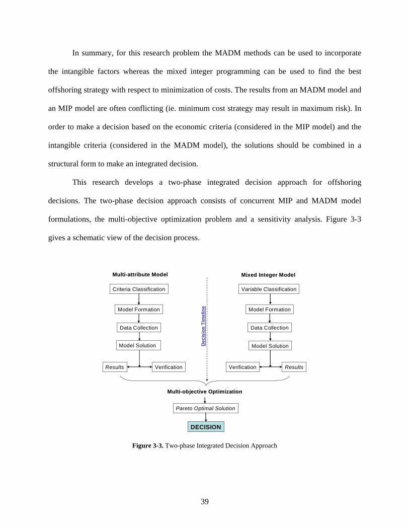
39
In summary, for this research problem the MADM methods can be used to incorporate
the intangible factors whereas the mixed integer programming can be used to find the best
offshoring strategy with respect to minimization of costs. The results from an MADM model and
an MIP model are often conflicting (ie. minimum cost strategy may result in maximum risk). In
order to make a decision based on the economic criteria (considered in the MIP model) and the
intangible criteria (considered in the MADM model), the solutions should be combined in a
structural form to make an integrated decision.
This research develops a two-phase integrated decision approach for offshoring
decisions. The two-phase decision approach consists of concurrent MIP and MADM model
formulations, the multi-objective optimization problem and a sensitivity analysis. Figure 3-3
gives a schematic view of the decision process.
Criteria Classification
Model Formation
Data Collection
Results Verification
Variable Classification
Model Formation
Data Collection
Model Solution
ResultsVerification
MultiMulti--attribute Modelattribute Model Mixed Integer ModelMixed Integer Model
MultiMulti--objective Optimizationobjective Optimization
Pareto Optimal Solution
DECISION
Dec
isio
n Ti
mel
ine
Model Solution
Figure 3-3. Two-phase Integrated Decision Approach

40
The MIP model includes quantitative data whereas the MADM model includes
qualitative factors. These models are independent of each other, therefore can be formed
concurrently. The results of the models are entered into a multi-objective programming problem
that yields a set of Pareto optimal solutions. The decision maker decides on the best offshoring
strategy by evaluating the tradeoffs.
These two phases are presented in detail by first giving an overview of the methodologies
used and then describing the model implementation in offshoring decisions. Selection of the
specific tools (MIP and ANP) is also justified. After the illustration of the two phases, the
integration process is presented.
3.3 MIXED INTEGER PROGRAMMING
3.3.1 Background
Mixed integer programming is a generalization of linear programming in which some of the
decision variables are constrained to be integers. Many production and location problems are
solved as mixed integer programs due to the existence of fixed charges. These are incurred
whenever the activity (i.e. production, transportation) is undertaken. Examples of fixed charges
are setup costs, location rental costs and minimum order quantities. Furthermore, integer values
can also enter into a linear programming model to deal with “if-then” constraints and piecewise
linear functions. Piecewise linear functions can occur as a result of such situations such as price
discounts depending on order quantities and cost reductions due to economies of scale and
training.
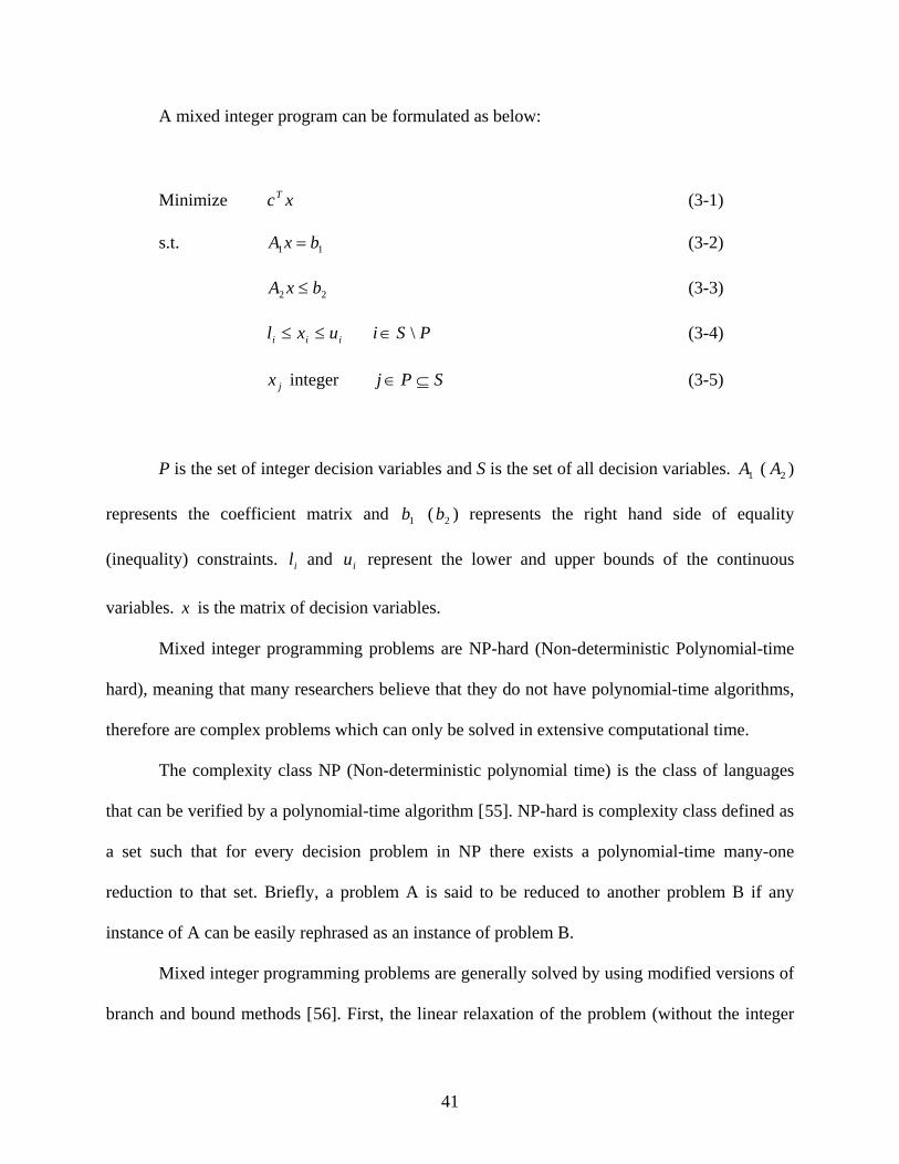
41
A mixed integer program can be formulated as below:
Minimize xcT (3-1)
s.t. 11 bxA = (3-2)
22 bxA ≤ (3-3)
iii uxl ≤≤ PSi \∈ (3-4)
jx integer SPj ⊆∈ (3-5)
P is the set of integer decision variables and S is the set of all decision variables. 1A ( 2A )
represents the coefficient matrix and 1b ( 2b ) represents the right hand side of equality
(inequality) constraints. il and iu represent the lower and upper bounds of the continuous
variables. x is the matrix of decision variables.
Mixed integer programming problems are NP-hard (Non-deterministic Polynomial-time
hard), meaning that many researchers believe that they do not have polynomial-time algorithms,
therefore are complex problems which can only be solved in extensive computational time.
The complexity class NP (Non-deterministic polynomial time) is the class of languages
that can be verified by a polynomial-time algorithm [55]. NP-hard is complexity class defined as
a set such that for every decision problem in NP there exists a polynomial-time many-one
reduction to that set. Briefly, a problem A is said to be reduced to another problem B if any
instance of A can be easily rephrased as an instance of problem B.
Mixed integer programming problems are generally solved by using modified versions of
branch and bound methods [56]. First, the linear relaxation of the problem (without the integer
42
constraints) is solved to optimum. If the optimum solution happens to satisfy integer conditions,
it is the optimal for the MIP problem. If not, additional linear inequality constraints (called
cutting planes) are added to the system in such a way as to remove the suboptimal extreme point
solution. There are several methods of building cutting planes including Gomory’s cuts [57] and
Lift-and-Project cuts [58]. Although MIP problems are difficult to solve, branch and bound
algorithms have been successful in providing optimal solutions.
On the other hand, for large MIP problems optimality may be too difficult to obtain
because of the computational complexity. In some cases, optimality may even be unnecessary
due to the problem’s nature. In these cases, heuristic methods are applied either to obtain a near-
optimum solution or to accelerate the branch and bound method by reducing the number of
iterations to approach the exact optimum. A well known heuristic is Pivot and Shift developed
by Balas et al. [59]. It is an extension to general mixed integer programming of Pivot and
Complement which is a heuristic for finding approximate solutions to binary programming
problems. Tabu search and genetic algorithms are also widely used in developing general
heuristics for MIP problems. A tabu search based method for binary MIP is presented by
Lokketangen and Glover [60] whereas Kostikas and Fragakis [61] apply genetic programming to
MIP by embedding the genetic run into the branch and bound process.
Mixed integer programming is applied to many real life problems: one of its biggest
application areas is in supply chain management. In production planning, integer values are
required to take into account setup times. Problems that are formulated mixed integer
programming include lot sizing [62], production and staff scheduling [63, 64], site location [65]
and transportation [66] problems. Supplier selection in supply chains is mathematically similar
to site location and transportation problems. Due to the existence of both fixed and variables
43
costs, the formulation of this problem is also structured as mixed integer programming. Total
cost of production/ownership approach is also incorporated while modeling the decision
mathematically.
3.3.2 Model
Possible alternative locations for manufacturing/services are considered as supply nodes and
possible locations of product/service sales are considered as demand nodes. Each arc between the
supply and demand points is represented by a variable denoting the volume of
manufacturing/service supplied from the supply point to the demand point. In addition, a binary
variable is associated with each supply node, representing the existence of manufacturing/service
in that location. A general formulation for global supplier selection problem can be structured as
an MIP model.
Indices:
I: Set of supply points - Ii ∈ represents a supply point
J: Set of demand points- Jj ∈ represents a demand point
T: Time horizon (annually divided: t = one year) - Tt ∈ represents a one year period
Decision variables:
tijx = amount of production/service at supplier i and transported to location j (for consumption) at
year t
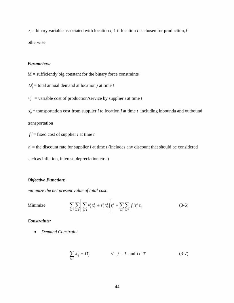
44
iz = binary variable associated with location i, 1 if location i is chosen for production, 0
otherwise
Parameters:
M = sufficiently big constant for the binary force constraints
tjD = total annual demand at location j at time t
tiv = variable cost of production/service by supplier i at time t
tijs = transportation cost from supplier i to location j at time t including inbounda and outbound
transportation
tif = fixed cost of supplier i at time t
tir = the discount rate for supplier i at time t (includes any discount that should be considered
such as inflation, interest, depreciation etc..)
Objective Function:
minimize the net present value of total cost:
Minimize ∑ ∑∑∑ ∑∈ ∈ ∈∈ ∈
+⎥⎦
⎤⎢⎣
⎡+
Iii
Ii Tt
ti
ti
ti
Tt Jj
tij
tij
tij
ti zrfrxsxv (3-6)
Constraints:
• Demand Constraint
tj
Ii
tij Dx =∑
∈
∀ Jj ∈ and Tt ∈ (3-7)
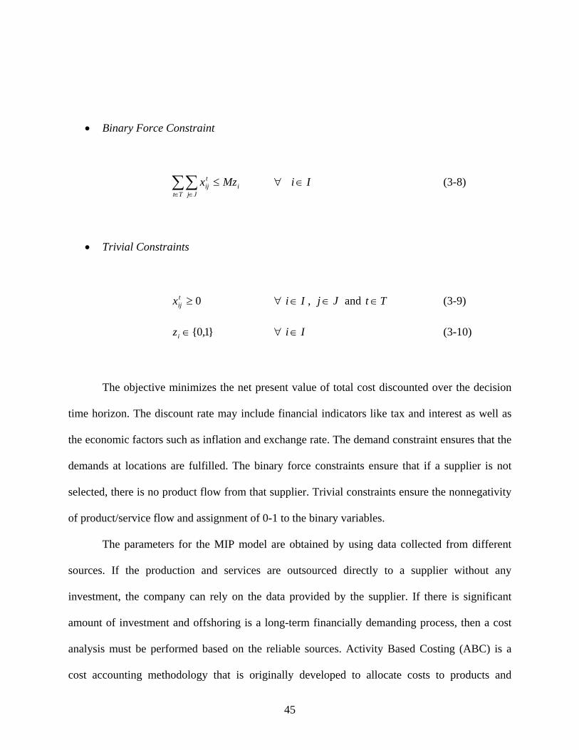
45
• Binary Force Constraint
iTt Jj
tij Mzx ≤∑∑
∈ ∈
∀ Ii ∈ (3-8)
• Trivial Constraints
0≥tijx ∀ Ii ∈ , Jj ∈ and Tt ∈ (3-9)
}1,0{∈iz ∀ Ii ∈ (3-10)
The objective minimizes the net present value of total cost discounted over the decision
time horizon. The discount rate may include financial indicators like tax and interest as well as
the economic factors such as inflation and exchange rate. The demand constraint ensures that the
demands at locations are fulfilled. The binary force constraints ensure that if a supplier is not
selected, there is no product flow from that supplier. Trivial constraints ensure the nonnegativity
of product/service flow and assignment of 0-1 to the binary variables.
The parameters for the MIP model are obtained by using data collected from different
sources. If the production and services are outsourced directly to a supplier without any
investment, the company can rely on the data provided by the supplier. If there is significant
amount of investment and offshoring is a long-term financially demanding process, then a cost
analysis must be performed based on the reliable sources. Activity Based Costing (ABC) is a
cost accounting methodology that is originally developed to allocate costs to products and
46
services. ABC identifies the activities and consumed resources and determines the cost variables
according to the relationship between activities, products/services and consumed resources. This
technique is also utilized to estimate costs by using basic resource costs (i.e. electricity, labor) to
develop the product/service cost.
The MIP model can be solved via various commercial solvers or by developing a solution
algorithm specifically for the problem. In this research, the MIP models are sparse without many
decision variables. Thus, there is no need to develop a specific solution algorithm, rather
commercial solvers can be utilized. Hence, the ILOG Cplex 9.0 with C programming language
interface is used to solve the MIP problem. Cplex uses branch and cut to solve MIP models [67].
It begins by solving the relaxation of the model: i.e., all integrality constraints and special order
sets are ignored. It proceeds by introducing the integrality constraints one by one. Branching
from a parent node occurs as bounds are modified and cuts occur as new constraints are added.
As a result, the solution of the MIP model gives the optimal choice of alternatives and
production/service distributions with respect to minimization of costs.
3.4 ANALYTIC NETWORK PROCESS
3.4.1 Background
In this research Analytic Network Process (ANP) is selected as the MADM method in the
integrated two-phase methodology. As discussed, the ANP is an advanced decision making
technique that is based on the fundamental principles of Analytical Hierarchy Process (AHP). In
fact, AHP is a special case of ANP, where the elements are assumed to be independent of each
47
other. ANP is structured on the same basis of AHP, but it does not assume independence
between criteria and alternatives [68]. ANP can capture complex decision making problems by
incorporating a feedback mechanism and attribute interactions as well as the hierarchical
relationship of alternatives. Multiple expert and multiple criteria features of decision making
problems are intelligently tied together to formulate a network of elements.
According to Saaty [69], there are three elements to a decision problem: goal, criteria and
alternatives. Interactions between these three elements can be defined in a tree structure. Both
AHP and ANP evaluate the alternatives with a bottom-to-top approach. AHP formulates decision
models in a single hierarchy whereas ANP has a network structure with sub-networks where the
criteria are divided into sub models. Dependencies between criteria and alternatives are handled
with feedback mechanisms. In the sub-networks, the feedback mechanism ensures a more
realistic reflection of the intrinsic complexity of organizational decisions. In general, the basic
reasoning behind AHP and ANP are the same. Although the structure of the model is more
complex in ANP, both are based on “comparative judgments.”
Intangible values are quantified using the proposition of ratio scales and the criteria are
compared based on the priority theory. That is, a comparison between two elements is made
according to the intensity (how much?) and dominance (which one?). The priorities of criteria
determine the weight factors in the goal. The comparisons are made by experts/stakeholders. For
a case with n criteria, n(n-1)/2 pair-wise comparisons are made with respect to a common
attribute by each expert. The control mechanism for the consistency of judgments in the
comparisons is the “inconsistency factor” which is calculated from the comparison matrix. The
comparison ratios are entered in a comparison matrix and the priorities are obtained by
48
calculating the eigenvector of this matrix. The priorities represent the conversion of the paired
comparisons of the criteria into a ratio scale.
The steps for building an ANP model start with structuring the network that consists of
hierarchies and dependencies. The goal is considered to be the root of the network, where the
alternatives are assessed by their Benefit, Opportunity, Cost and Risk (BOCR) influences with
respect to the goal. The combination of the goal and its relationship with the major criteria is
called the “control hierarchy.” Under each parent criterion (BOCR), sub-networks are built
according to the specific conditions of the problem. These sub-networks are further divided into
sub-criteria which are connected to different stakeholders. The feedback structure is essential to
ANP and is the element that differentiates ANP from AHP. It represents interactions that
converge toward the goal. Under sub-networks feedback loops can be added to stakeholders and
criteria nodes. Once the network structure is completed, the decision maker (or makers)
performs the paired comparisons between the attributes with respect to their parent criteria.
The fundamental scale of ANP is based on absolute numbers which is described as the
ratio of ratio numbers. Absolute numbers are used to answer the basic question in all paired
comparisons: how many times more dominant is one element than the other with respect to a
certain criterion or attribute. Paired comparisons are always more precise than rating alternatives
independent of each other. Rating and ranking alternatives separately without the knowledge of
entire decision space will create biased solutions. If a person does not have a basis to judge
things relatively, s/he cannot give accurate scores, values or rankings. For instance, when a
person is asked how happy s/he is feeling at the moment, s/he will try to answer by comparing
her/his feelings with past experiences and judgments. Such a comparison is made by first
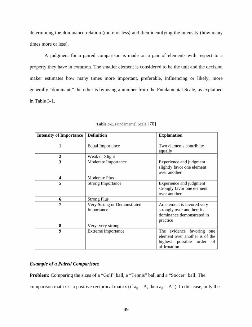
49
determining the dominance relation (more or less) and then identifying the intensity (how many
times more or less).
A judgment for a paired comparison is made on a pair of elements with respect to a
property they have in common. The smaller element is considered to be the unit and the decision
maker estimates how many times more important, preferable, influencing or likely, more
generally “dominant,” the other is by using a number from the Fundamental Scale, as explained
in Table 3-1.
Table 3-1. Fundamental Scale [70]
Intensity of Importance
Definition Explanation
1 Equal Importance Two elements contribute equally
2 Weak or Slight 3 Moderate Importance Experience and judgment
slightly favor one element over another
4 Moderate Plus 5 Strong Importance Experience and judgment
strongly favor one element over another
6 Strong Plus 7 Very Strong or Demonstrated
Importance An element is favored very strongly over another; its dominance demonstrated in practice
8 Very, very strong 9 Extreme importance The evidence favoring one
element over another is of the highest possible order of affirmation
Example of a Paired Comparison:
Problem: Comparing the sizes of a “Golf” ball, a “Tennis” ball and a “Soccer” ball. The
comparison matrix is a positive reciprocal matrix (if aij = A, then aji = A-1). In this case, only the

50
judgments for the upper or lower diagonal of the paired comparison matrix are needed. An
example is shown in Table 3-2.
Table 3-2. Paired Comparison Example
Golf Ball Tennis
Ball Soccer Ball Golf B. 1 3 8 Tennis B. 1/3 1 5 Soccer B. 1/8 1/5 1
For upper diagonal judgments, the questions are:
With respect to size:
1- How much bigger is a tennis ball than a golf ball?
Judgment: Moderately bigger (3)
2- How much bigger is a soccer ball than a golf ball?
Judgment: Very strongly bigger (8)
3- How much bigger is a soccer ball than a tennis ball?
Judgment: Strongly bigger (5)
One should note that the lower diagonal judgments are the reciprocals. For lower
diagonal, the questions will be:
1- How much smaller is a golf ball than a tennis ball?
Judgment: Moderately smaller (1/3)
2- How much smaller is a golf ball than an apple?
Judgment: Very strongly smaller (1/8)
3- How much smaller is a tennis ball than a soccer ball?
Judgment: Strongly smaller (1/5)
51
These kinds of comparisons require observation of sizes of the objects under
consideration. On the other hand, many of the real life decision problems necessitate comparison
of intangible values that are often subject to individual perspectives. For instance, instead of
comparing the sizes of the sports balls, one can ask to compare the popularity of these three
sports. Then, the judgments are based on subjective preferences as well as the data such as the
number of people who watch each sport. If such subjectivity needs to be minimized, the
comparisons should be done by multiple decision makers who have different perspectives and
whose collective judgments will be combined to yield a more objective result. However if by the
nature of the problem, the decision needs based on the preferences of the decision maker,
subjectivity is needed and favored.
Inconsistency in Paired Comparisons:
If a tennis ball is deemed three times bigger than a golf ball and a soccer ball is five times
bigger than a tennis ball, shouldn’t a soccer ball be 15 times bigger than a golf ball? Why is the
comparison value eight instead? Such inconsistency is natural in human thinking as long as it
does not exceed certain values. For ANP judgments, inconsistency under a certain value does not
yield a significant perturbation in the results. The consistency of a comparison matrix is
quantified by a “Consistency Index” which is a measure of deviation of matrix from consistency.
The formula for the consistency index is:1
max
−−
≡n
nλμ where maxλ is the principal (largest)
eigenvalue and n is the dimension of the matrix [71].
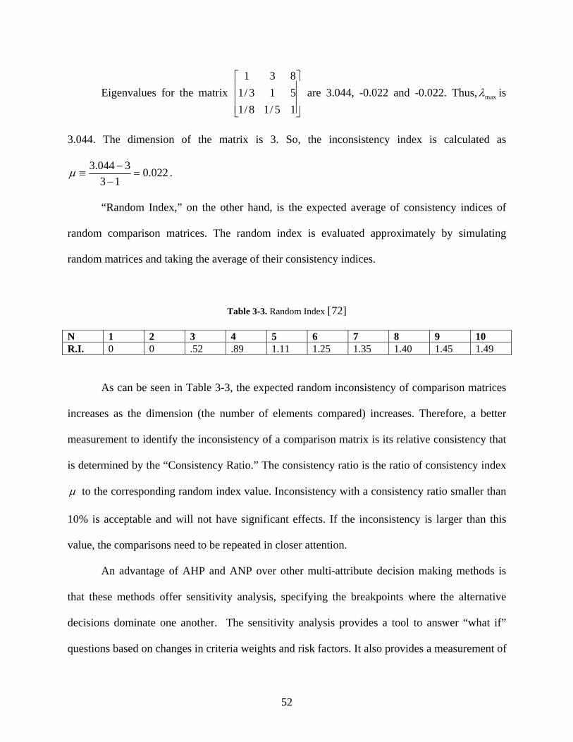
52
Eigenvalues for the matrix ⎥⎥⎥
⎦
⎤
⎢⎢⎢
⎣
⎡
15/18/1513/1831
are 3.044, -0.022 and -0.022. Thus, maxλ is
3.044. The dimension of the matrix is 3. So, the inconsistency index is calculated as
022.013
3044.3=
−−
≡μ .
“Random Index,” on the other hand, is the expected average of consistency indices of
random comparison matrices. The random index is evaluated approximately by simulating
random matrices and taking the average of their consistency indices.
Table 3-3. Random Index [72]
N 1 2 3 4 5 6 7 8 9 10 R.I. 0 0 .52 .89 1.11 1.25 1.35 1.40 1.45 1.49
As can be seen in Table 3-3, the expected random inconsistency of comparison matrices
increases as the dimension (the number of elements compared) increases. Therefore, a better
measurement to identify the inconsistency of a comparison matrix is its relative consistency that
is determined by the “Consistency Ratio.” The consistency ratio is the ratio of consistency index
μ to the corresponding random index value. Inconsistency with a consistency ratio smaller than
10% is acceptable and will not have significant effects. If the inconsistency is larger than this
value, the comparisons need to be repeated in closer attention.
An advantage of AHP and ANP over other multi-attribute decision making methods is
that these methods offer sensitivity analysis, specifying the breakpoints where the alternative
decisions dominate one another. The sensitivity analysis provides a tool to answer “what if”
questions based on changes in criteria weights and risk factors. It also provides a measurement of
53
sustainability and certainty of the final decision. Such an indicator suggests a scheme for the
overall decision and the frequency with which the decision making technique should be repeated
to check the optimality of the solution.
Another advantage of AHP and ANP is their ability to handle complex problems [73].
Complex decision problems consisting of dependent criteria and attributes are usually solved by
utilizing ANP whereas AHP is used for simpler problems with a hierarchical decision structure.
Application areas of ANP are numerous. Examples include R&D project selections [74], policy
planning [75], financial crisis forecasting [76] and supply chain management [77].
An important of benefit of AHP and ANP are their ease of implementation [78]. Many of
the other multi-criteria methods that are based on utility theory may be either too theoretical to
apply or too complex to be appropriate in a corporate decision process. The paired comparison
technique makes the methods easier to comprehend by decision makers.
AHP and ANP methods are sometimes criticized because of claims that the utility based
methodologies are better in terms of theory [79]. A major criticism is the possibility of “rank
reversal.” Rank reversal occurs when different alternatives are added to the problem and the
ranking of alternatives changes with this addition [80]. Another criticism is the large number of
paired comparisons that should be performed in the model solution. Especially as the number of
criteria increases, the number of paired comparisons escalates exponentially. The discussion on
the theory and applicability of multi-criteria decision making methods can further be expanded
[81] but is not pursued further in this research. Overall, the results of AHP and ANP have been
accepted in many problems and its applicability is demonstrated
Here ANP is selected because of its advantages and its applicability to corporate decision
making is demonstrated in many ways. The rank reversal and scale of paired comparisons are not
54
major concerns for the problems in consideration because the decision problem is a strategic
problem that does not require frequent computation and modification. Moreover, for the
complexity and the dependencies of criteria in the decision problem in consideration, using
utility based approaches is not practical, even if possible.
3.4.2 Model
In this research, the Analytic Network Process model is not used as a method to find the
solutions for a decision problem, rather it is used as a tool to quantify the intangible factors that
exist in an offshoring decision. As a result of offshoring, companies seek competitive advantage
by reducing the cost of their production and services. According to an Accenture survey of more
than 800 executives in the United States and Europe, cost savings are still a key offshoring
benefit, but the additional business controls generated by offshoring are driving the trend [82].
Offshoring comes with uncertainties and risks. For instance companies that transfer operations
overseas put their intellectual property and core competencies at risk.
Such intangible values involved in a decision model can broadly be classified into two
groups: “Opportunities” and “Risks.” Opportunities represent the short and long term benefits
that the company realizes as a result of the decision. Risks represent all the possible negative
results that may be incurred as a result of the decision. The magnitude of the risks and
opportunities that a company realizes is based on the supplier choice, the regions selected and the
volume of production and services that are moved overseas. Obviously this magnitude varies
depending on the execution of offshoring after the decision is made, but still a strategic
offshoring decision should be made to minimize the possible risks and maximize opportunities
by finding the best suppliers and the distribution of production/services.
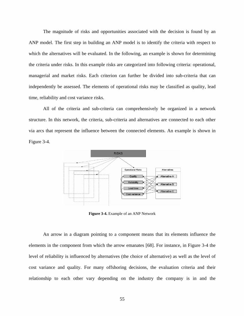
55
The magnitude of risks and opportunities associated with the decision is found by an
ANP model. The first step in building an ANP model is to identify the criteria with respect to
which the alternatives will be evaluated. In the following, an example is shown for determining
the criteria under risks. In this example risks are categorized into following criteria: operational,
managerial and market risks. Each criterion can further be divided into sub-criteria that can
independently be assessed. The elements of operational risks may be classified as quality, lead
time, reliability and cost variance risks.
All of the criteria and sub-criteria can comprehensively be organized in a network
structure. In this network, the criteria, sub-criteria and alternatives are connected to each other
via arcs that represent the influence between the connected elements. An example is shown in
Figure 3-4.
Figure 3-4. Example of an ANP Network
An arrow in a diagram pointing to a component means that its elements influence the
elements in the component from which the arrow emanates [68]. For instance, in Figure 3-4 the
level of reliability is influenced by alternatives (the choice of alternative) as well as the level of
cost variance and quality. For many offshoring decisions, the evaluation criteria and their
relationship to each other vary depending on the industry the company is in and the

56
product/service nature that will be outsourced. Thus, the criteria, sub-criteria and the structure of
the network should be considered for every offshoring decision separately.
After the formation of the network, the next step is to compare the elements based on
their importance. The comparisons are performed as a result of expert analyses. The generic
question is [70]: Given an element (in the same component or in another component) of the
system or given a component of that system, how much more does a second element
(component) of a pair influence that first element (component) with respect to a control sub
criterion (criterion)? The format of the question is based on the relations in the network model.
Priorities are derived from the paired comparisons by taking the matrix eigenvectors and
consequently these priorities are input to a supermatrix. The columns are weighted by priorities
of influence of corresponding components. Then the resulting column stochastic supermatrix is
multiplied by itself with a limit power to obtain the priorities of alternatives with respect to upper
level criteria. Their aggregation with the upper criteria weights gives the synthesized values of
the end result which is a ranking of alternatives. As a result of standardization of alternative
priorities, the solution to the problem can be obtained.
In offshoring decisions the paired comparisons should be based on company executives’
opinions, literature survey, expert reviews [83] and real data from such databases as
Countrywatch [84] and Sourceoecd [85]. Comparisons for country specific criteria may be
evaluated based on newspaper articles, consultant reports and Internet search. Various reports are
published to point out competitive indices for countries, which can be used as a basis for
evaluating suppliers depending on their locations. Moreover historical economic data, such as
inflation rates, can be used as an indicator for stability of resources. Supplier specific
57
comparisons, on the other hand, need individuals who can assess the suppliers based on their
experiences.
The ANP model gives opportunity and risk weights associated with each offshoring
(supplier or in-house/offshore location) alternative. Alternatives are denoted in the set I = {i = 1,
…, n}. The quantified risk associated with alternative i obtained from the ANP model is denoted
as iR whereas the opportunity is denoted as iO .
3.5 INTEGRATION
Multi-attribute decision making methods may be used to determine the best alternative for a
complex decision problem that includes intangible and tangible values. However, continuous
variables such as production amounts cannot be included in a multi-attribute model. On the other
hand, mathematical models give precise optimum answers by considering continuous and
discrete decision spaces as well as production/service constraints. Yet, they cannot include
intangible values that have complex interactive relations. This research combines the strengths of
these two methods by integrating them to develop an approach based on multi-objective
optimization.
3.5.1 Background
Most of the decision problems in real life have multiple conflicting objectives. Multiple
objectives can be optimized by utilizing multi-objective optimization techniques that generate
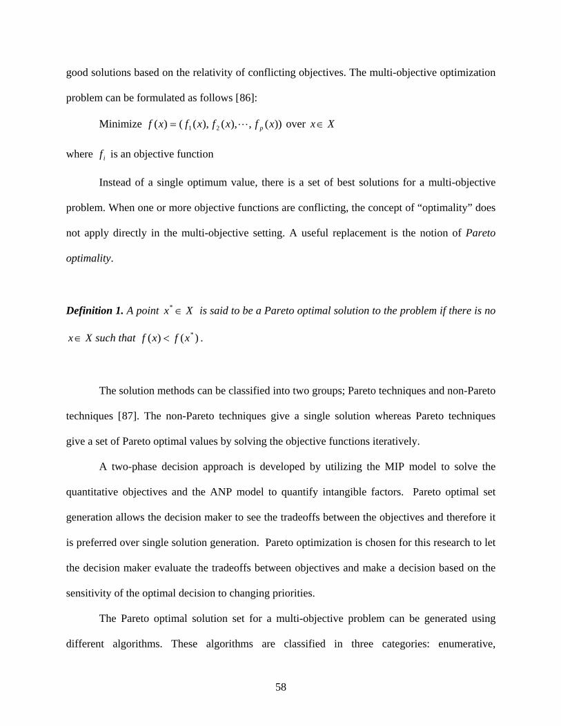
58
good solutions based on the relativity of conflicting objectives. The multi-objective optimization
problem can be formulated as follows [86]:
Minimize ))(,),(),(()( 21 xfxfxfxf pL= over Xx ∈
where if is an objective function
Instead of a single optimum value, there is a set of best solutions for a multi-objective
problem. When one or more objective functions are conflicting, the concept of “optimality” does
not apply directly in the multi-objective setting. A useful replacement is the notion of Pareto
optimality.
Definition 1. A point Xx ∈* is said to be a Pareto optimal solution to the problem if there is no
Xx ∈ such that )()( *xfxf < .
The solution methods can be classified into two groups; Pareto techniques and non-Pareto
techniques [87]. The non-Pareto techniques give a single solution whereas Pareto techniques
give a set of Pareto optimal values by solving the objective functions iteratively.
A two-phase decision approach is developed by utilizing the MIP model to solve the
quantitative objectives and the ANP model to quantify intangible factors. Pareto optimal set
generation allows the decision maker to see the tradeoffs between the objectives and therefore it
is preferred over single solution generation. Pareto optimization is chosen for this research to let
the decision maker evaluate the tradeoffs between objectives and make a decision based on the
sensitivity of the optimal decision to changing priorities.
The Pareto optimal solution set for a multi-objective problem can be generated using
different algorithms. These algorithms are classified in three categories: enumerative,

59
deterministic, and stochastic [88]. Stochastic methods include heuristic search algorithms such as
tabu search, simulated annealing and evolutionary algorithms. Extensive research has been
carried out in recent years in the area of evolutionary algorithms [89]. These algorithms utilize
the Darwinian evolutionary theory to generate a near-to-optimal population by eliminating the
unfit points and reproducing from the fit ones. The advantage of stochastic methods is their
ability to find good solutions for large size problems in a reasonable amount of time. The
disadvantage is that they do not guarantee optimal solutions and their performance depends on
many factors such as the initial population and adjustment parameters.
On the other hand, deterministic algorithms guarantee optimal solutions and give
solutions on the exact Pareto space. For instance, gradient based algorithms and branch and
bound methods can provide exact Pareto values. Enumerative search algorithms are based on
evaluating each possible solution from a given finite search space. For problems with a finite
solution space, enumerative search algorithms can actually give the exact Pareto set.
Computationally enumerative search algorithms are expensive, requiring exhaustive optimization
of objective functions in many iterations.
Another classification of multi-objective optimization methods can be done based on the
articulation of preferences [90]. “No articulation of preferences” methods generally combine the
objective functions in an aggregate function called a global criterion. Examples are: weighted-
sum, compromise programming and min-max methods. “A priori articulation of preferences”
methods include preferences of the decision maker in the optimization approach. Lexicographic
and hierarchical methods involve ordering of objectives according their relative importance.
Many of the “no articulation of preferences” methods such as the weighted-sum method can also
be modified with the preferences. “A posteriori articulation of preferences” methods such as the
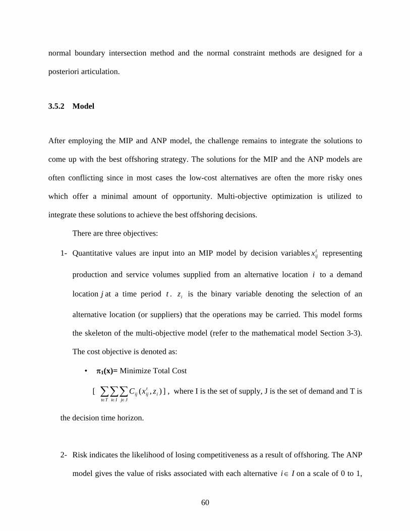
60
normal boundary intersection method and the normal constraint methods are designed for a
posteriori articulation.
3.5.2 Model
After employing the MIP and ANP model, the challenge remains to integrate the solutions to
come up with the best offshoring strategy. The solutions for the MIP and the ANP models are
often conflicting since in most cases the low-cost alternatives are often the more risky ones
which offer a minimal amount of opportunity. Multi-objective optimization is utilized to
integrate these solutions to achieve the best offshoring decisions.
There are three objectives:
1- Quantitative values are input into an MIP model by decision variables tijx representing
production and service volumes supplied from an alternative location i to a demand
location j at a time period t . iz is the binary variable denoting the selection of an
alternative location (or suppliers) that the operations may be carried. This model forms
the skeleton of the multi-objective model (refer to the mathematical model Section 3-3).
The cost objective is denoted as:
• π1(x)= Minimize Total Cost
[ ∑∑∑∈ ∈ ∈Tt Ii Jj
itijij zxC ),( ] , where I is the set of supply, J is the set of demand and T is
the decision time horizon.
2- Risk indicates the likelihood of losing competitiveness as a result of offshoring. The ANP
model gives the value of risks associated with each alternative Ii ∈ on a scale of 0 to 1,
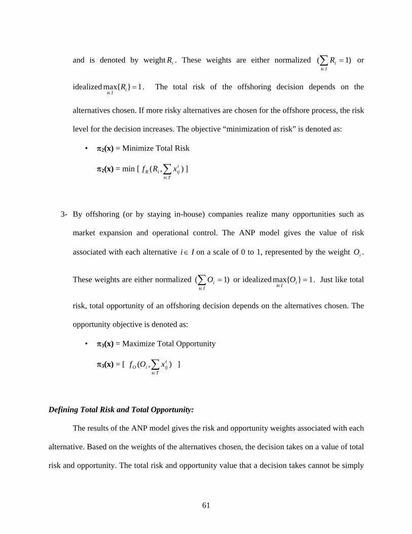
61
and is denoted by weight iR . These weights are either normalized )1( =∑∈Ii
iR or
idealized 1}{max =∈ iIi
R . The total risk of the offshoring decision depends on the
alternatives chosen. If more risky alternatives are chosen for the offshore process, the risk
level for the decision increases. The objective “minimization of risk” is denoted as:
• π2(x) = Minimize Total Risk
π2(x) = min [ ),( ∑∈Tt
tijiR xRf ]
3- By offshoring (or by staying in-house) companies realize many opportunities such as
market expansion and operational control. The ANP model gives the value of risk
associated with each alternative Ii ∈ on a scale of 0 to 1, represented by the weight iO .
These weights are either normalized )1( =∑∈Ii
iO or idealized 1}{max =∈ iIi
O . Just like total
risk, total opportunity of an offshoring decision depends on the alternatives chosen. The
opportunity objective is denoted as:
• π3(x) = Maximize Total Opportunity
π3(x) = [ ),( ∑∈Tt
tijiO xOf ]
Defining Total Risk and Total Opportunity:
The results of the ANP model gives the risk and opportunity weights associated with each
alternative. Based on the weights of the alternatives chosen, the decision takes on a value of total
risk and opportunity. The total risk and opportunity value that a decision takes cannot be simply

62
defined as the sum of risk and opportunity weights of the alternatives chosen because this value
not only depends on the alternatives but also depends on the nature of the risk and opportunity.
For instance, if the risk involved in an offshore process compromises mainly the risk of losing
intellectual property rights, doing business with an additional supplier will add more to the total
risk. On the other hand, if the risk compromises mainly the risk of tardiness in production,
working with diverse set of suppliers will mitigate the level of risk in the process.
In this study, the total risk and opportunity is defined with an analogy from the portfolio
management literature in finance. In finance, the total risk of a portfolio is defined as the sum of
systematic (nondiversifiable) and unsystematic (diversifiable) risks [91]. The unsystematic risk
is the risk that can be “washed out” by diversification, such as organizational changes that affect
only the stocks of a company. The systematic risk is the risk which cannot be diversified away,
such as sudden fluctuations in interest rates and inflation.
number of shares
Risk
5 10 15
Unsystematic Risk
Systematic Risk
Figure 3-5. Portfolio Risk [92]
Analogous to the portfolio risk definition, as depicted in Figure 3-5, in this study risks (or
opportunities) are defined as the sum of diversifiable and nondiversifiable risks (or
opportunities). Diversifiable risks are risks that can be alleviated by distributing the production
or services to multiple locations and suppliers. Risks related to lead time, macro-economic

63
conditions (ie. interest and inflation) and quality are diversifiable. Diversifiable opportunities are
opportunities that are elevated by distributing the production or services to multiple locations,
such as opportunities for future product development, price reduction opportunities and quality
enhancements. On the other hand, nondiversifiable risks are risks that add up as more locations
are in the supply chain. These include intellectual property risks, implementation risks and
management risks. Nondiversifiable opportunities are opportunities that reduce as the production
or services are distributed. For instance, market expansion is an opportunity directly proportional
to the company’s share which is based on the volume of production and services in the region.
Within this framework, the total of diversifiable risks (or nondiversifiable opportunities)
is defined as the sum of individual location risks (or opportunities) weighted by the volume of
production and services at each location. The total of nondiversifiable risks (or diversifiable
opportunities) is defined as the unweighted sum of individual location risks (or opportunities).
Once the total risk and opportunity functions are determined, a multi-objective problem is
formulated consisting of the three objectives and the necessary constraints related to the
offshoring decision. This multi-objective problem is characterized by the following:
• Preference articulation is very difficult without any information about the trade-offs
between the objectives. Moreover, the preferences depend not only on the value of the
objectives but also on the amount of production/services. Therefore, a method that can be
solved without any prior preference articulation is needed.
• In order to show the decision maker the trade-offs, a Pareto optimal solution set needs to
be generated. The Pareto optimal solution set can be plotted as a three dimensional graph
with each axis representing one of the objectives. Visualization of the optimal set helps
the decision maker to see the tradeoffs and make a sound decision based on preferences.
64
• The decision of offshoring usually consists of a small set of a limited number of location
alternatives. Therefore, the multi-objective optimization problem is a small sized problem
that does not necessitate the use of any heuristic optimization methods.
• The objectives for “risks” and “opportunities” have limits determined by the minimum
and maximum risk and opportunity values of the alternatives. Moreover these bounds are
numerically restricted due to the fact that risk and opportunity quantifications must be
between 0 and 1. This feature puts bounds on the search space and creates computational
advantage.
The preferences need to be elucidated a posteriori and due to the small size of the
problem, exact methods are computationally efficient enough to solve such a multi-objective
problem. Therefore two methods are selected to generate the Pareto front: weighted-sum and
epsilon-constraint methods.
Weighted-sum method:
The weighted-sum method is a scalarization method that aggregates the objectives with
associated weights and generates the Pareto optimal points by solving the aggregated objective.
The weighted-sum method is a traditional multi-objective optimization method that is used for
various applications. The multi-objective problem is converted into a scalar problem by
constructing a weighted sum of all objectives. In the literature the weights are often used to
represent preferences, however in cases without any preference articulation the weights can be
used to generate the Pareto front. This also eliminates any problems that can come into play due
to the deficiencies of using weights as preference indicators.
If each objective is denoted by min )(xFi s.t. Xx ∈ for i = 1, … , n

65
The weighted-sum approach solves the problem as follows:
min )(xFwi
ii∑ s.t. Xx ∈
Pareto optimal solutions are obtained by changing the weights. Minimizing the weighted-
sum is a necessary condition for Pareto optimality if the feasible region is convex [93].
Moreover, if 0>iw for all i, minimizing the weighted-sum is a sufficient condition,
guaranteeing that the solutions are always Pareto optimal [94].
If weighted-sum method is used for the multi-objective problem considered in this
research, the cost objective function would dominate the aggregated objective function because
of its relatively large value. In order to prevent one function’s domination due to different orders
of magnitude, transformations must be performed. There are various function transformation
methods in the literature. Marler [90] presents an exhaustive review and comparison of these
methods. As a conclusion, the author proposes that using the upper-lower-bound approach can
improve the performance of the weighted-sum method and using this approach with Pareto-
maximum values provides superior results. Therefore, this method is recommended as a function
transformation approach. Moreover, using convex combination of weights is also recommended
to facilitate a Pareto front with more uniformly scattered optimal points.
Epsilon-constraint method:
The epsilon-constraint method is not a scalarization approach; rather it is in a class called
bounded objective function methods. It solves one of the objective functions (primary objective
function) by adding the other objective functions into the constraint space. The Pareto optimal
points are generated by changing the constraint limits of the objectives.

66
If the primary objective is denoted by min )(xFs and all other objectives are denoted by min
)(xFi ; within the total constraint set Xx ∈ then the epsilon-constraint approach solves the
problem:
min )(xFs s.t. Xx ∈ and ii xF ε≤)( for si ≠
The point that minimizes the primary objective function is denoted by *sx .
Epsilon limit selection can be made by two methods that ensure the satisfaction of Pareto-
optimality conditions. These are “primary-objective” and “pareto-maximum” methods. The
primary-objective approach restricts the epsilons as [95]: )( *0siii xFF ≤≤ ε where the Pareto-
maximum approach replaces )( *si xF with the Pareto-maximum of iF . 0
iF represents the
minimum of function i and )( *si xF is the value of function i at *
sx . The Pareto-maximum approach
is found to give better results when compared to the primary-objective method, however the
points found may sometimes be weak Pareto-optimal (not unique) [96].
In terms of computational efficiency and the quality of the results, both methods have
advantages and disadvantages. The weighted-sum method can generate different optimal points
at each iteration (by changing the weights) whereas the epsilon-constraint method encounters
infeasibility or duplication in some iterations. The epsilon-constraint method does not need any
normalization whereas the weighted-sum approach needs extra computation time due to the
necessity for using transformation functions.
For the specific problem discussed in this research, the epsilon-constraint method is able
to cover the constraint space with less iterations because of the distinct property that the two
objectives have, specifically risks and opportunity objectives are limited by the maximum and
minimum values of risks and opportunities of the alternatives. However research suggests [90]
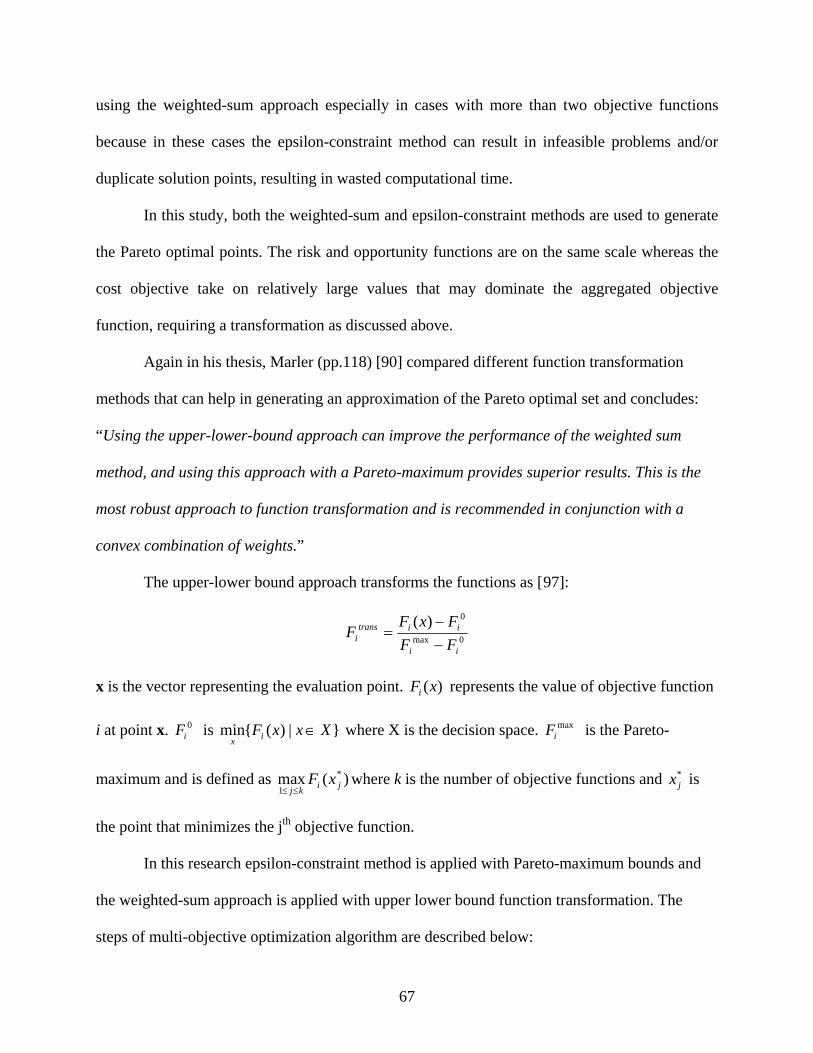
67
using the weighted-sum approach especially in cases with more than two objective functions
because in these cases the epsilon-constraint method can result in infeasible problems and/or
duplicate solution points, resulting in wasted computational time.
In this study, both the weighted-sum and epsilon-constraint methods are used to generate
the Pareto optimal points. The risk and opportunity functions are on the same scale whereas the
cost objective take on relatively large values that may dominate the aggregated objective
function, requiring a transformation as discussed above.
Again in his thesis, Marler (pp.118) [90] compared different function transformation
methods that can help in generating an approximation of the Pareto optimal set and concludes:
“Using the upper-lower-bound approach can improve the performance of the weighted sum
method, and using this approach with a Pareto-maximum provides superior results. This is the
most robust approach to function transformation and is recommended in conjunction with a
convex combination of weights.”
The upper-lower bound approach transforms the functions as [97]:
0max
0)(
ii
iitransi FF
FxFF
−−
=
x is the vector representing the evaluation point. )(xFi represents the value of objective function
i at point x. 0iF is }|)({min XxxFix
∈ where X is the decision space. maxiF is the Pareto-
maximum and is defined as )(max *
1 jikjxF
≤≤where k is the number of objective functions and *
jx is
the point that minimizes the jth objective function.
In this research epsilon-constraint method is applied with Pareto-maximum bounds and
the weighted-sum approach is applied with upper lower bound function transformation. The
steps of multi-objective optimization algorithm are described below:
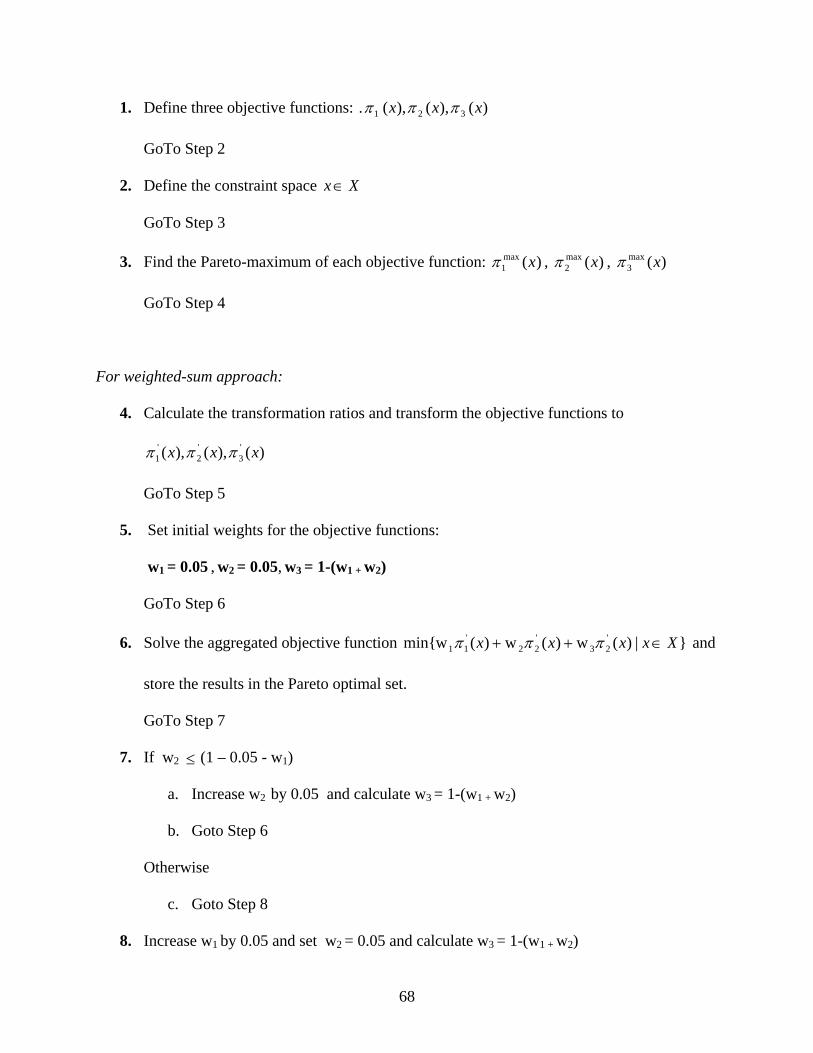
68
1. Define three objective functions: )(),(),( . 321 xxx πππ
GoTo Step 2
2. Define the constraint space Xx ∈
GoTo Step 3
3. Find the Pareto-maximum of each objective function: )(max1 xπ , )(max
2 xπ , )(max3 xπ
GoTo Step 4
For weighted-sum approach:
4. Calculate the transformation ratios and transform the objective functions to
)(),(),( '3
'2
'1 xxx πππ
GoTo Step 5
5. Set initial weights for the objective functions:
w1 = 0.05 , w2 = 0.05, w3 = 1-(w1 + w2)
GoTo Step 6
6. Solve the aggregated objective function }|)(w)(w)(wmin{ '23
'22
'11 Xxxxx ∈++ πππ and
store the results in the Pareto optimal set.
GoTo Step 7
7. If w2 ≤ (1 – 0.05 - w1)
a. Increase w2 by 0.05 and calculate w3 = 1-(w1 + w2)
b. Goto Step 6
Otherwise
c. Goto Step 8
8. Increase w1 by 0.05 and set w2 = 0.05 and calculate w3 = 1-(w1 + w2)
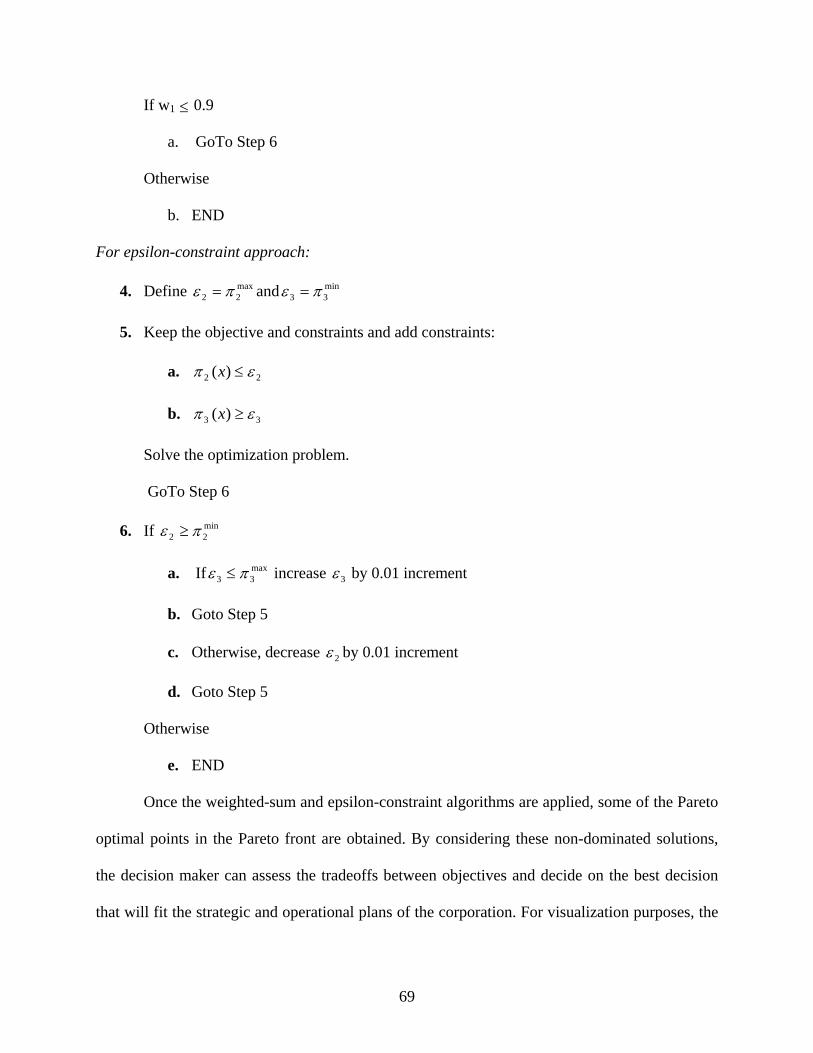
69
If w1 ≤ 0.9
a. GoTo Step 6
Otherwise
b. END
For epsilon-constraint approach:
4. Define max22 πε = and min
33 πε =
5. Keep the objective and constraints and add constraints:
a. 22 )( επ ≤x
b. 33 )( επ ≥x
Solve the optimization problem.
GoTo Step 6
6. If min22 πε ≥
a. If max33 πε ≤ increase 3ε by 0.01 increment
b. Goto Step 5
c. Otherwise, decrease 2ε by 0.01 increment
d. Goto Step 5
Otherwise
e. END
Once the weighted-sum and epsilon-constraint algorithms are applied, some of the Pareto
optimal points in the Pareto front are obtained. By considering these non-dominated solutions,
the decision maker can assess the tradeoffs between objectives and decide on the best decision
that will fit the strategic and operational plans of the corporation. For visualization purposes, the

70
decision maker may be assisted by plotting the Pareto set in a three dimensional graph where
each axis represents one of the objectives. Furthermore, sensitivity analysis and utility elicitation
may be performed to analyze the tradeoffs and make a final decision with respect to the
preferences of the decision maker.

71
4.0 OFFSHORE OUTSOURCING EMPIRICAL STUDY: SIMA
SIMA Products Corporations is a private company which was founded in 1973 and as of 2006
operates in Oakmont, Pennsylvania [98]. SIMA is a leading innovator of consumer electronic
accessories. It designs and creates consumer electronics and sells products to major retailers in
the U.S. market, such as Best Buy and Circuit City. The company started as a small family
business in the photographic accessories industry. Over the years, SIMA has developed a large
supply network consisting of several suppliers around the world as well as its retail network,
which has included not only category-killers like Circuit City and Best Buy, but also niche
players such as Ricoh and local merchandisers.
SIMA is competitive in the consumer electronics industry characterized by very short
product cycles, rapidly changing market opportunities, and a subtle balance of cooperation and
rivalry with suppliers and retailers. Their business model is based on the early identification of
niche market opportunities—typically targeted at highly sophisticated users of mainstream
consumer electronics—that are often too small to be of interest to large consumer electronics
companies. Once the market opportunity is identified, the product has to be designed and
manufactured within a very short period of time. One of the paradoxes of the business is that if a
product turns out to be really successful, it becomes attractive to SIMA’s retailers, who may then
see an opportunity to produce a similar product themselves, rather than to carry SIMA’s product.
Given that product life cycles are so short that a product’s sales begin declining even before the
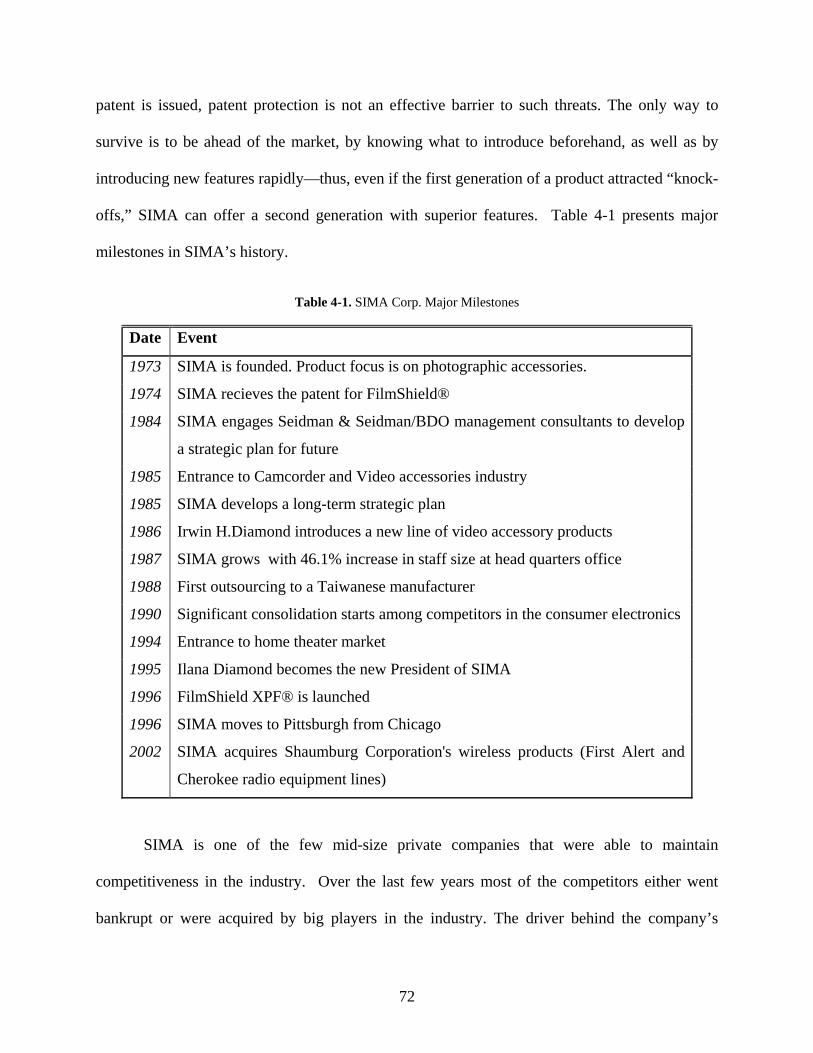
72
patent is issued, patent protection is not an effective barrier to such threats. The only way to
survive is to be ahead of the market, by knowing what to introduce beforehand, as well as by
introducing new features rapidly—thus, even if the first generation of a product attracted “knock-
offs,” SIMA can offer a second generation with superior features. Table 4-1 presents major
milestones in SIMA’s history.
Table 4-1. SIMA Corp. Major Milestones
Date Event
1973 SIMA is founded. Product focus is on photographic accessories.
1974 SIMA recieves the patent for FilmShield®
1984 SIMA engages Seidman & Seidman/BDO management consultants to develop
a strategic plan for future
1985 Entrance to Camcorder and Video accessories industry
1985 SIMA develops a long-term strategic plan
1986 Irwin H.Diamond introduces a new line of video accessory products
1987 SIMA grows with 46.1% increase in staff size at head quarters office
1988 First outsourcing to a Taiwanese manufacturer
1990 Significant consolidation starts among competitors in the consumer electronics
1994 Entrance to home theater market
1995 Ilana Diamond becomes the new President of SIMA
1996 FilmShield XPF® is launched
1996 SIMA moves to Pittsburgh from Chicago
2002 SIMA acquires Shaumburg Corporation's wireless products (First Alert and
Cherokee radio equipment lines)
SIMA is one of the few mid-size private companies that were able to maintain
competitiveness in the industry. Over the last few years most of the competitors either went
bankrupt or were acquired by big players in the industry. The driver behind the company’s

73
success has been its innovation business model that the company has kept as a core competence
even while profit margins in the electronic equipment industry were under pressure and the rate
of product obsolescence continued to accelerate.
The fierce price competition caused by the power shift in the supply chain, forced
companies towards a search for less costly manufacturing opportunities. During the 1980s, the
first signs of the offshore outsourcing trend were apparent with the rising manufacturing
capabilities in Taiwan. The offshore outsourcing scheme became common in 1990s and today
most consumer electronics items are manufactured outside the United States. SIMA was one of
the earliest companies to outsource its manufacturing tasks to Taiwan in late 1980s. At that time,
only the mature products that needed mass production were candidates for offshore outsourcing.
Today, the competition is so strong that offshore outsourcing is necessarily considered for every
product regardless of its phase in the product life cycle.
Working with offshore suppliers for manufacturing of products creates competitive
advantages such as lower product costs and increased concentration on innovation. However it
also creates many problems which may lead to monetary losses as well as withdrawals from the
market. For instance, SIMA had to exit the remote control market because of an unreliable
supplier even though the market in the U.S. had significant business opportunities. Past
experiences showed that the suppliers in Hong Kong and Taiwan are usually more trustworthy in
protecting the intellectual property and maintaining quality control. On the other hand, these
suppliers cannot offer prices as low as the suppliers in China. Chinese suppliers have the
advantages of economies of scale, low raw material costs and labor rates; however they tend to
work with larger companies that can copy the innovative designs of SIMA. Another tradeoff is
between product costs and engineering capabilities. In the past, SIMA has experienced many
74
instances where the products failed only because of miscommunication and lack of technical
expertise of suppliers. The market is very sensitive to price and at the same time customers
demand innovation and superior design. Therefore, it is important to work with suppliers which
can provide high quality engineering services while ensuring a competitive market price for the
product. For SIMA, it is a big challenge to choose suppliers which can provide both low costs
and the high innovative capability that the market seeks.
Although cost is an important determinant in supplier selection, it is only one of the
factors that determine the success of the product. Through the past years, the bad and good
experiences taught SIMA that measures that are not tangible like technology capability should be
a consideration before starting a business with a supplier. SIMA has classified these qualitative
variables under the criterion “experience” because experience seems to be the only standard for
these variables. However, experience by itself cannot be easily measured and it does not reflect
all of the intangible factors that should go into a supplier selection process. In this research, the
qualitative and quantitative measures that should go into the supplier selection decisions of
SIMA are investigated and an integrated systematic decision approach is illustrated for the
selection of a supplier (offshore and inshore) that would manufacture a new product line
designed by SIMA.
In the consumer electronic industry the product life cycles are short, usually ranging from
six months to one year. A major challenge in supplier selection for a consumer electronic product
is the demand fluctuations at each product life cycle phase. SIMA experienced several cases of
their product becoming obsolete when big players entered the market with a similar product
(often with a copied design) and reduced product prices. In the first phase where the product is
launched and the demand grows, the most crucial thing is to protect the design from competitors.
75
Once the product is on the shelf for a certain length of time and is successful, it is inevitably
copied and then price becomes the major factor in competition. Consequently the demand for the
product changes drastically. Therefore, in this research a decision model is built for offshore
supplier selection by assuming different demand volumes. The model shows how the decision
changes depending on the demand volume. This enables the decision makers to conduct scenario
analysis by considering possible outcomes.
As described in the methodology section, the decision approach is implemented in two
phases. First, a mathematical model is formulated to evaluate the quantitative variables involved
in the decision. This model finds the best supplier alternative(s) and the distribution of
manufacturing among the suppliers with respect to the financial considerations. Later, the
qualitative variables are identified and classified into criteria groups. The supplier alternatives
are evaluated with respect to these criteria by constructing an ANP model. The results are later
synthesized to generate the best strategy in terms of both quantitative and qualitative variables.
The process in consideration for offshore outsourcing is the manufacturing of High-
Definition Multimedia Interface (HDMI) switchers. HDMI switchers are used to connect
multiple devices such as play stations and DVD players to one HD (high definition) monitor.
There are three product lines: 2x1 HDMI (with two inputs), 3x1 HDMI (with three inputs) and
5x1 HDMI (with five inputs). Four supplier alternatives are evaluated in terms of their monetary
advantageousness as well as the risks and opportunities they engender.

76
4.1 MATHEMATICAL MODEL FOR SIMA CORPORATION
4.1.1 Model Formulation
The mathematical formulation is a supplier selection model with four possible supplier
alternatives, one demand point and three products. The supplier alternatives are: Amberson
(Taiwan), Function (U.S.A.), NTC (Hong Kong) and Belton (Peoples Republic of China). The
real names of the suppliers have been disguised to protect the confidentiality. The products will
be sold only in the U.S. market, thus there is one demand point and all of the manufactured
products will be shipped to the U.S. The total demand is difficult to estimate before the product
is launched because the demand can fluctuate depending on the product life phase. However, the
proportions of sales for each product line can reliably be estimated based on the current market
information. The mathematical model minimizes the total relevant cost incurred in product
purchases from suppliers.
Assumptions:
• The product life cycle is short (less than one year) and therefore time variables (such as
interest rate) are ignored.
• The capacities of the suppliers are adequate to meet total demand.
• The minimum quantity that can be ordered is 500 units.
Indices:
I: {i = 1,2,3.4} Set of supply points
P: {p = 1,2,3} Set of product types
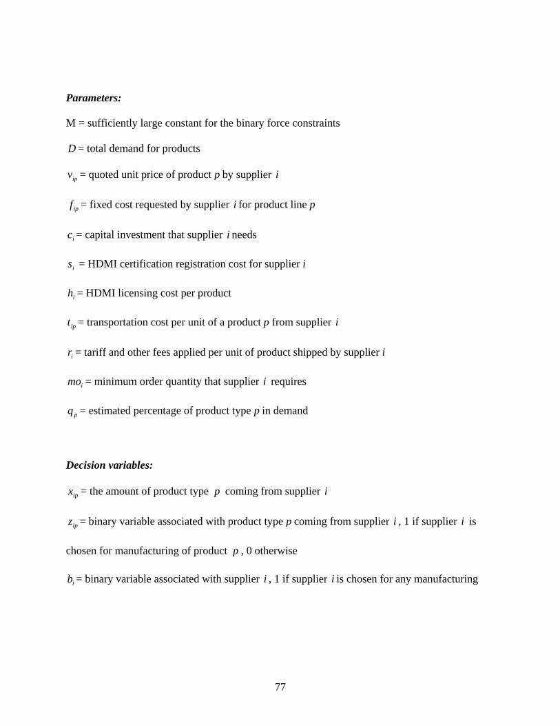
77
Parameters:
M = sufficiently large constant for the binary force constraints
D = total demand for products
ipv = quoted unit price of product p by supplier i
ipf = fixed cost requested by supplier i for product line p
ic = capital investment that supplier i needs
is = HDMI certification registration cost for supplier i
ih = HDMI licensing cost per product
ipt = transportation cost per unit of a product p from supplier i
ir = tariff and other fees applied per unit of product shipped by supplier i
imo = minimum order quantity that supplier i requires
pq = estimated percentage of product type p in demand
Decision variables:
ipx = the amount of product type p coming from supplier i
ipz = binary variable associated with product type p coming from supplier i , 1 if supplier i is
chosen for manufacturing of product p , 0 otherwise
ib = binary variable associated with supplier i , 1 if supplier i is chosen for any manufacturing
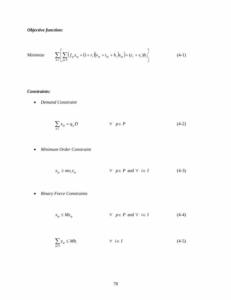
78
Objective function:
Minimize ( )( )( )∑ ∑∈ ∈
⎥⎦
⎤⎢⎣
⎡++++++
Ii Ppiiiipiipipiipip bscxhtvrzf )(1 (4-1)
Constraints:
• Demand Constraint
Dqx pIi
ip =∑∈
∀ Pp ∈ (4-2)
• Minimum Order Constraint
ipiip zmox ≥ ∀ Pp ∈ and ∀ Ii ∈ (4-3)
• Binary Force Constraints
ipip Mzx ≤ ∀ Pp ∈ and ∀ Ii ∈ (4-4)
∑∈
≤Pp
iip Mbz ∀ Ii ∈ (4-5)
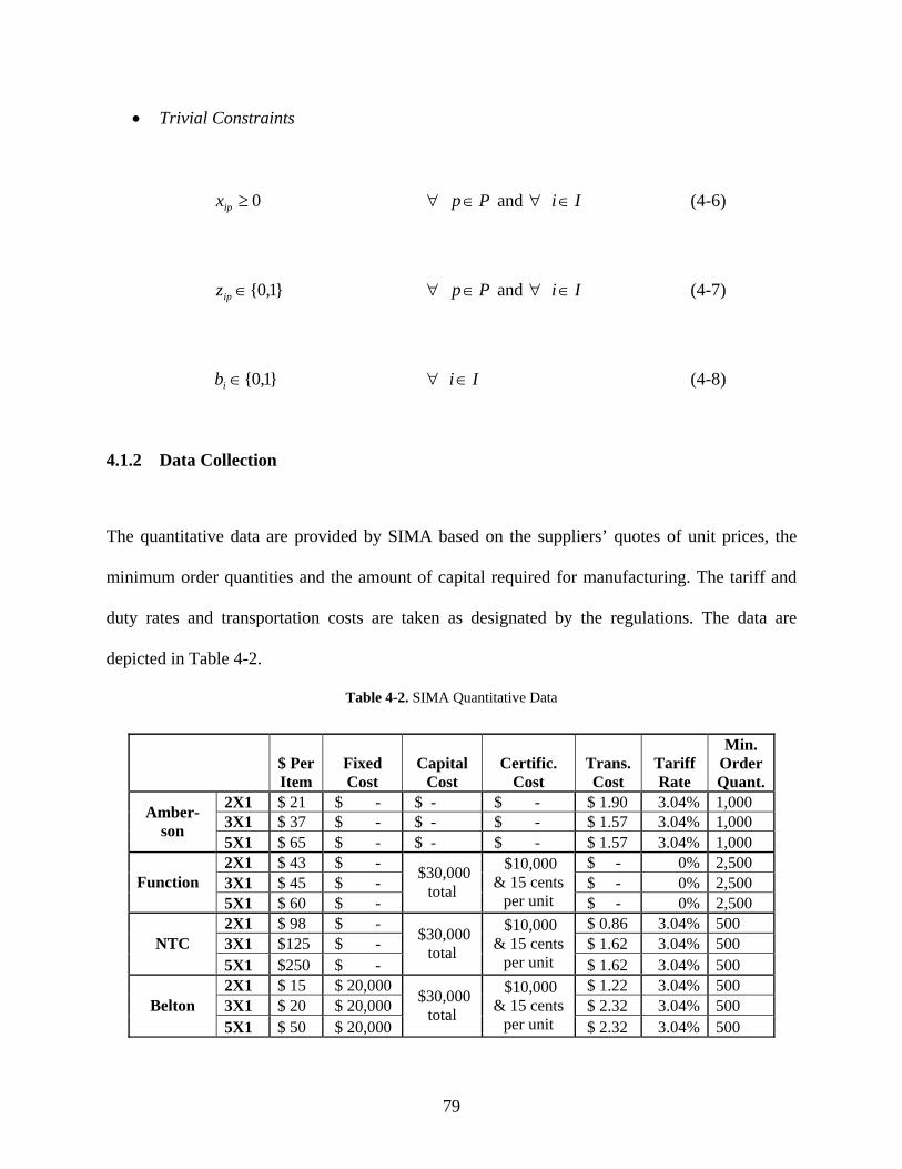
79
• Trivial Constraints
0≥ipx ∀ Pp ∈ and ∀ Ii ∈ (4-6)
}1,0{∈ipz ∀ Pp ∈ and ∀ Ii ∈ (4-7)
}1,0{∈ib ∀ Ii ∈ (4-8)
4.1.2 Data Collection
The quantitative data are provided by SIMA based on the suppliers’ quotes of unit prices, the
minimum order quantities and the amount of capital required for manufacturing. The tariff and
duty rates and transportation costs are taken as designated by the regulations. The data are
depicted in Table 4-2.
Table 4-2. SIMA Quantitative Data
$ Per Item
Fixed Cost
Capital Cost
Certific. Cost
Trans. Cost
Tariff Rate
Min. Order Quant.
2X1 $ 21 $ - $ - $ - $ 1.90 3.04% 1,000 3X1 $ 37 $ - $ - $ - $ 1.57 3.04% 1,000 Amber-
son 5X1 $ 65 $ - $ - $ - $ 1.57 3.04% 1,000 2X1 $ 43 $ - $ - 0% 2,500 3X1 $ 45 $ - $ - 0% 2,500 Function 5X1 $ 60 $ -
$30,000 total
$10,000 & 15 cents
per unit $ - 0% 2,500 2X1 $ 98 $ - $ 0.86 3.04% 500 3X1 $125 $ - $ 1.62 3.04% 500 NTC 5X1 $250 $ -
$30,000 total
$10,000 & 15 cents
per unit $ 1.62 3.04% 500 2X1 $ 15 $ 20,000 $ 1.22 3.04% 500 3X1 $ 20 $ 20,000 $ 2.32 3.04% 500 Belton 5X1 $ 50 $ 20,000
$30,000 total
$10,000 & 15 cents
per unit $ 2.32 3.04% 500

80
As indicated by SIMA, capacity is not a subject of consideration for the four alternative
suppliers because demand usually does not exceed the amount a large supplier can supply.
Belton requires SIMA to pay an extra tooling cost equivalent to $20,000 that will be used to buy
new equipment for each product line. The capital cost includes all the costs incurred for
additional resources and R&D involved in production. Amberson absorbs all of the capital cost
(depreciation, maintenance etc.) whereas the other three suppliers ask for approximately $30,000
for capital. In this case regardless of the amount of products supplied, $30,000 needs to be paid.
LLC is the licensing agent responsible for administering the licensing of the HDMI
specification, promoting the HDMI standard and providing education on the benefits of HDMI to
retailers and consumers [99]. HDMI adopter manufacturers have licensing rights for their end
products in return to registering with HDMI Licensing and cooperating with the HDMI standards
and tests. The first HDMI product produced by a manufacturer in each device category must be
tested at an HDMI Authorized Testing Center. The registration fee for being an HDMI adopter is
$10,000 per year and an additional 15 cents is paid per unit sold. SIMA has a policy asking for
HDMI certification for all of the devices they sell in the U.S. market. Since the life cycle of the
product is not expected to be more than one year, $10,000 is listed as the certification cost and
the quoted unit prices are increased by 15 cents for suppliers who are not registered with HDMI
Licensing.
The transportation cost includes the ocean freight and land transportation of the product
from the supplier. Function has agreed to ship the product with no charge. The same tariff rate
applies to shipments whether they are from mainland China (PRC), Taiwan or Hong Kong. The
tariff rate is 2.7% of total value (rounded to nearest dollar) of the shipment. An additional 0.21%
merchandise processing fee and 0.125% harbor maintenance fee is charged for ocean shipments.
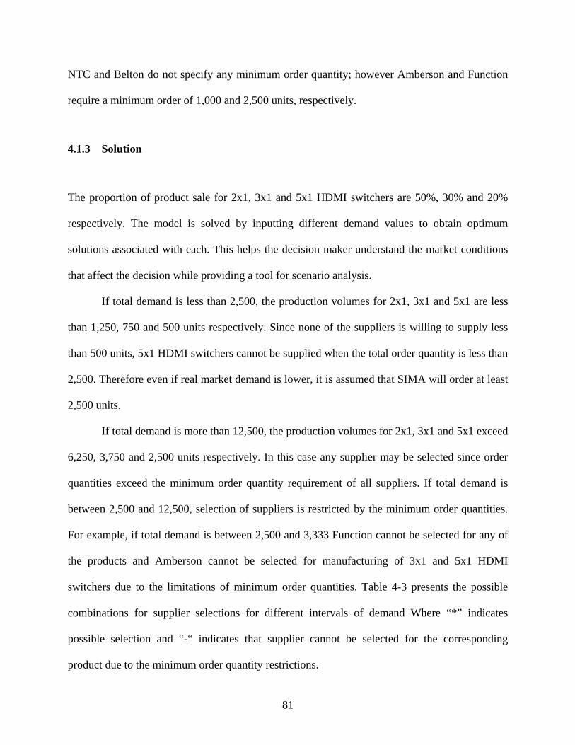
81
NTC and Belton do not specify any minimum order quantity; however Amberson and Function
require a minimum order of 1,000 and 2,500 units, respectively.
4.1.3 Solution
The proportion of product sale for 2x1, 3x1 and 5x1 HDMI switchers are 50%, 30% and 20%
respectively. The model is solved by inputting different demand values to obtain optimum
solutions associated with each. This helps the decision maker understand the market conditions
that affect the decision while providing a tool for scenario analysis.
If total demand is less than 2,500, the production volumes for 2x1, 3x1 and 5x1 are less
than 1,250, 750 and 500 units respectively. Since none of the suppliers is willing to supply less
than 500 units, 5x1 HDMI switchers cannot be supplied when the total order quantity is less than
2,500. Therefore even if real market demand is lower, it is assumed that SIMA will order at least
2,500 units.
If total demand is more than 12,500, the production volumes for 2x1, 3x1 and 5x1 exceed
6,250, 3,750 and 2,500 units respectively. In this case any supplier may be selected since order
quantities exceed the minimum order quantity requirement of all suppliers. If total demand is
between 2,500 and 12,500, selection of suppliers is restricted by the minimum order quantities.
For example, if total demand is between 2,500 and 3,333 Function cannot be selected for any of
the products and Amberson cannot be selected for manufacturing of 3x1 and 5x1 HDMI
switchers due to the limitations of minimum order quantities. Table 4-3 presents the possible
combinations for supplier selections for different intervals of demand Where “*” indicates
possible selection and “-“ indicates that supplier cannot be selected for the corresponding
product due to the minimum order quantity restrictions.
82
Table 4-3. SIMA Supplier Selection Possibilities
Minimum 1,250 1,667 2,500 4,167 Maximum 1,667 2,500 4,167 6,250 Amberson * * * * Function - - * * NTC * * * *
2x1 HDMI
Belton * * * * Minimum 750 1,000 1,500 2,500 Maximum 1,000 1,500 2,500 3,750 Amberson - * * * Function - - - * NTC * * * *
3x1 HDMI
Belton * * * * Minimum 500 667 1,000 1,667 Maximum 667 1,000 1,667 2,500 Amberson - - * * Function - - - - NTC * * * *
5x1 HDMI
Belton * * * * Minimum 2,500 3,333 5,000 8,333 Total
Demand Maximum 3,333 5,000 8,333 12,500
Belton’s unit price quotes are lower than that of Amberson, Function and NTC and
Belton requires a lower minimum order quantity. When compared with NTC and Function, the
only drawback of choosing Belton would be the tooling cost which is $20,000 per production
line. Breakeven analyses are performed to determine how much production volume is needed in
order for Belton to incur a total cost that is less than that of what Function and NTC.
Figure 4-1 illustrates that if production volume is more than 240 units, when compared to
NTC, Belton’s tooling cost for the 2x1 HDMI production line is recovered by its lower unit
costs.
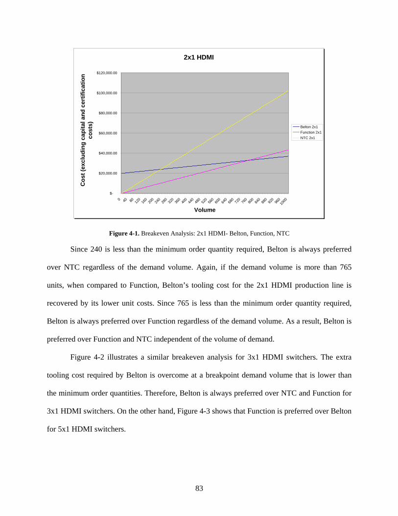
83
2x1 HDMI
$-
$20,000.00
$40,000.00
$60,000.00
$80,000.00
$100,000.00
$120,000.00
0 40 80 120
160
200
240
280
320
360
400
440
480
520
560
600
640
680
720
760
800
840
880
920
960
1000
Volume
Cos
t (ex
clud
ing
capi
tal a
nd c
ertif
icat
ion
cost
s) Belton 2x1Function 2x1NTC 2x1
Figure 4-1. Breakeven Analysis: 2x1 HDMI- Belton, Function, NTC
Since 240 is less than the minimum order quantity required, Belton is always preferred
over NTC regardless of the demand volume. Again, if the demand volume is more than 765
units, when compared to Function, Belton’s tooling cost for the 2x1 HDMI production line is
recovered by its lower unit costs. Since 765 is less than the minimum order quantity required,
Belton is always preferred over Function regardless of the demand volume. As a result, Belton is
preferred over Function and NTC independent of the volume of demand.
Figure 4-2 illustrates a similar breakeven analysis for 3x1 HDMI switchers. The extra
tooling cost required by Belton is overcome at a breakpoint demand volume that is lower than
the minimum order quantities. Therefore, Belton is always preferred over NTC and Function for
3x1 HDMI switchers. On the other hand, Figure 4-3 shows that Function is preferred over Belton
for 5x1 HDMI switchers.

84
3x1 HDMI
$-
$20,000.00
$40,000.00
$60,000.00
$80,000.00
$100,000.00
$120,000.00
$140,000.00
0 40 80 120
160
200
240
280
320
360
400
440
480
520
560
600
640
680
720
760
800
840
880
920
960
1000
Volume
Cos
t(exc
ludi
ng c
apita
l and
cer
tific
atio
n co
sts) Belton 3x1
Function 3x1NTC 3x1
Figure 4-2. Breakeven Analysis:3x1 HDMI - Belton,Function, NTC
5x1 HDMI
$-
$100,000.00
$200,000.00
$300,000.00
$400,000.00
$500,000.00
$600,000.00
$700,000.00
0 95 190
285
380
475
570
665
760
855
950
1045
1140
1235
1330
1425
1520
1615
1710
1805
1900
1995
2090
2185
2280
2375
2470
Volume
Cos
t(exc
ludi
ng c
aptia
l and
cer
tific
atio
n co
sts) Belton 5x1
Function 5x1NTC 5x1
Figure 4-3. Breakeven Analysis: 5x1 HDMI- Belton, Function, NTC
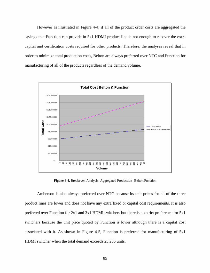
85
However as illustrated in Figure 4-4, if all of the product order costs are aggregated the
savings that Function can provide in 5x1 HDMI product line is not enough to recover the extra
capital and certification costs required for other products. Therefore, the analyses reveal that in
order to minimize total production costs, Belton are always preferred over NTC and Function for
manufacturing of all of the products regardless of the demand volume.
Total Cost Belton & Function
$-
$20,000.00
$40,000.00
$60,000.00
$80,000.00
$100,000.00
$120,000.00
$140,000.00
$160,000.00
$180,000.00
0 40 80 120
160
200
240
280
320
360
400
440
480
520
560
600
640
680
720
760
800
840
880
920
960
100
Volume
Tota
l Cos
t
Total BeltonBelton & 5x1 Function
Figure 4-4. Breakeven Analysis: Aggregated Production- Belton,Function
Amberson is also always preferred over NTC because its unit prices for all of the three
product lines are lower and does not have any extra fixed or capital cost requirements. It is also
preferred over Function for 2x1 and 3x1 HDMI switchers but there is no strict preference for 5x1
switchers because the unit price quoted by Function is lower although there is a capital cost
associated with it. As shown in Figure 4-5, Function is preferred for manufacturing of 5x1
HDMI switcher when the total demand exceeds 23,255 units.
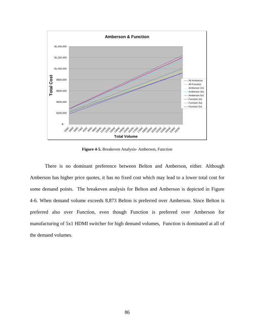
86
Amberson & Function
$-
$200,000
$400,000
$600,000
$800,000
$1,000,000
$1,200,000
$1,400,000
5000
5800
6600
7400
8200
9000
9800
1060
011
40012
20013
00013
80014
60015
40016
20017
00017
80018
60019
40020
20021
00021
80022
60023
40024
200
Total Volume
Tota
l Cos
t
All AmbersonAll FunctionAmberson 2x1Amberson 3x1Amberson 5x1Function 2x1Function 3x1Function 5x1
Figure 4-5. Breakeven Analysis- Amberson, Function
There is no dominant preference between Belton and Amberson, either. Although
Amberson has higher price quotes, it has no fixed cost which may lead to a lower total cost for
some demand points. The breakeven analysis for Belton and Amberson is depicted in Figure
4-6. When demand volume exceeds 8,873 Belton is preferred over Amberson. Since Belton is
preferred also over Function, even though Function is preferred over Amberson for
manufacturing of 5x1 HDMI switcher for high demand volumes, Function is dominated at all of
the demand volumes.
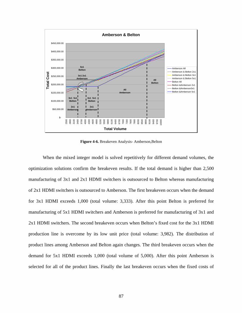
87
Amberson & Belton
$-
$50,000.00
$100,000.00
$150,000.00
$200,000.00
$250,000.00
$300,000.00
$350,000.00
$400,000.00
$450,000.00
2500
2800
3100
3400
3700
4000
4300
4600
4900
5200
5500
5800
6100
6400
6700
7000
7300
7600
7900
8200
8500
8800
9100
9400
9700
1000
0
Total Volume
Tota
l Cos
t
Amberson AllAmberson & Belton 2x1Amberson & Belton 3x1Amberson & Belton 5x1Belton AllBelton &Amberson 2x1Belton &Amberson3x1Belton &Amberson 5x1
3x1 5x1Belton
2x1 Amberson
5x1Belton
3x1 2x1 Amberson
3x1 5x1Belton
2x1 Amberson
AllAmberson
AllBelton
Figure 4-6. Breakeven Analysis- Amberson,Belton
When the mixed integer model is solved repetitively for different demand volumes, the
optimization solutions confirm the breakeven results. If the total demand is higher than 2,500
manufacturing of 3x1 and 2x1 HDMI switchers is outsourced to Belton whereas manufacturing
of 2x1 HDMI switchers is outsourced to Amberson. The first breakeven occurs when the demand
for 3x1 HDMI exceeds 1,000 (total volume: 3,333). After this point Belton is preferred for
manufacturing of 5x1 HDMI switchers and Amberson is preferred for manufacturing of 3x1 and
2x1 HDMI switchers. The second breakeven occurs when Belton’s fixed cost for the 3x1 HDMI
production line is overcome by its low unit price (total volume: 3,982). The distribution of
product lines among Amberson and Belton again changes. The third breakeven occurs when the
demand for 5x1 HDMI exceeds 1,000 (total volume of 5,000). After this point Amberson is
selected for all of the product lines. Finally the last breakeven occurs when the fixed costs of
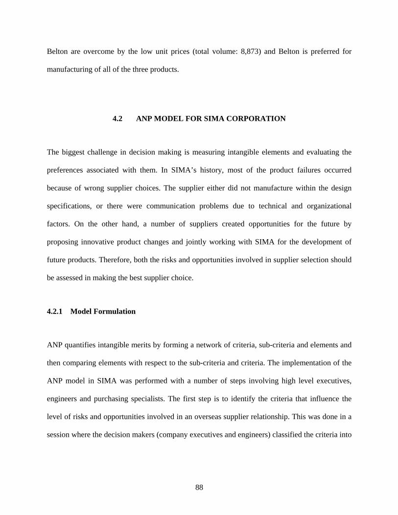
88
Belton are overcome by the low unit prices (total volume: 8,873) and Belton is preferred for
manufacturing of all of the three products.
4.2 ANP MODEL FOR SIMA CORPORATION
The biggest challenge in decision making is measuring intangible elements and evaluating the
preferences associated with them. In SIMA’s history, most of the product failures occurred
because of wrong supplier choices. The supplier either did not manufacture within the design
specifications, or there were communication problems due to technical and organizational
factors. On the other hand, a number of suppliers created opportunities for the future by
proposing innovative product changes and jointly working with SIMA for the development of
future products. Therefore, both the risks and opportunities involved in supplier selection should
be assessed in making the best supplier choice.
4.2.1 Model Formulation
ANP quantifies intangible merits by forming a network of criteria, sub-criteria and elements and
then comparing elements with respect to the sub-criteria and criteria. The implementation of the
ANP model in SIMA was performed with a number of steps involving high level executives,
engineers and purchasing specialists. The first step is to identify the criteria that influence the
level of risks and opportunities involved in an overseas supplier relationship. This was done in a
session where the decision makers (company executives and engineers) classified the criteria into
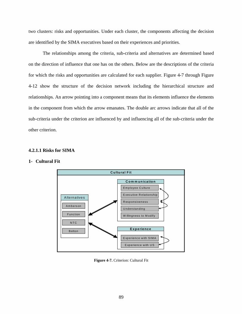
89
two clusters: risks and opportunities. Under each cluster, the components affecting the decision
are identified by the SIMA executives based on their experiences and priorities.
The relationships among the criteria, sub-criteria and alternatives are determined based
on the direction of influence that one has on the others. Below are the descriptions of the criteria
for which the risks and opportunities are calculated for each supplier. Figure 4-7 through Figure
4-12 show the structure of the decision network including the hierarchical structure and
relationships. An arrow pointing into a component means that its elements influence the elements
in the component from which the arrow emanates. The double arc arrows indicate that all of the
sub-criteria under the criterion are influenced by and influencing all of the sub-criteria under the
other criterion.
4.2.1.1 Risks for SIMA
1- Cultural Fit
C u ltu ra l F it
A m b ers on
Func tion
N T C
B elton
A lte rna tive s
A m b ers on
Func tion
N T C
B elton
A lte rna tive s
E xp erienc e w ith S IM A
E xp erienc e w ith U S
E xp erience
E xp erienc e w ith S IM A
E xp erienc e w ith U S
E xp erience
E m p loye e C u ltu re
E xecu tive R ela tionsh ip
C o m m un ica tio n
R esp ons iven ess
U nd ers tan d in g
W illingn ess to M odif y
E m p loye e C u ltu re
E xecu tive R ela tionsh ip
C o m m un ica tio n
R esp ons iven ess
U nd ers tan d in g
W illingn ess to M odif y
Figure 4-7. Criterion: Cultural Fit

90
a) Communication
i. Understanding: When SIMA requests changes in the product such as replacing a part of
an electronic device, the supplier should be able to recognize that the reason behind this
request is to make the product more marketable. If the supplier is having a hard time in
perceiving the needs of the U.S. market and SIMA’s efforts to modify product designs to
fulfill these needs, then the risk of having delays in the product development increases.
ii. Employee culture (western mind): Organizational culture is an important indicator of
how successful the relationship can be with a supplier. An Asian protocol is often
characterized by multi-level, hierarchical organizational structure that may slow down
decision processes.
iii. Responsiveness: Rapid response times to the requests made by SIMA are critical. The
product life cycles are so short that any delay in the production process may result in loss
of the entire market.
iv. Executive relationships: A close relationship between the executives generates trust at
high levels. This is especially true when conducting business in the Far East where the
president (or the CEO) of the company has direct command of the shop floor.
v. Willingness to modify: The supplier should be willing to modify the product in the
direction of SIMA’s request, even if the modification demands major work in the
manufacturing process.

91
b) Experience
i. Experience with U.S. companies: Suppliers that have worked with U.S. companies
should know the appropriate business procedures. Experience with other U.S. companies
mitigates the risks that arise due to the cultural differences.
ii. Experience with SIMA: Suppliers who have worked with SIMA previously know
SIMA’s expectations and requirements. Also, the risks involved with these suppliers can
be foreseen and action can be taken to prevent problems.
2- Technical Fit
Technical Fit
Amberson
Function
NTC
Belton
Alternatives
Amberson
Function
NTC
Belton
Alternatives
Ability to Modify
Engineering Team
Technical Fit
Experience withSimilar Products
Technical Resources
Figure 4-8. Criterion: Technical Fit
i. Ability to complete modifications: A supplier’s technical expertise should be sufficient
to perform product modifications.
ii. Experience with similar product lines: The more experience a supplier has with similar
products, the less is the probability that manufacturing problems will appear.
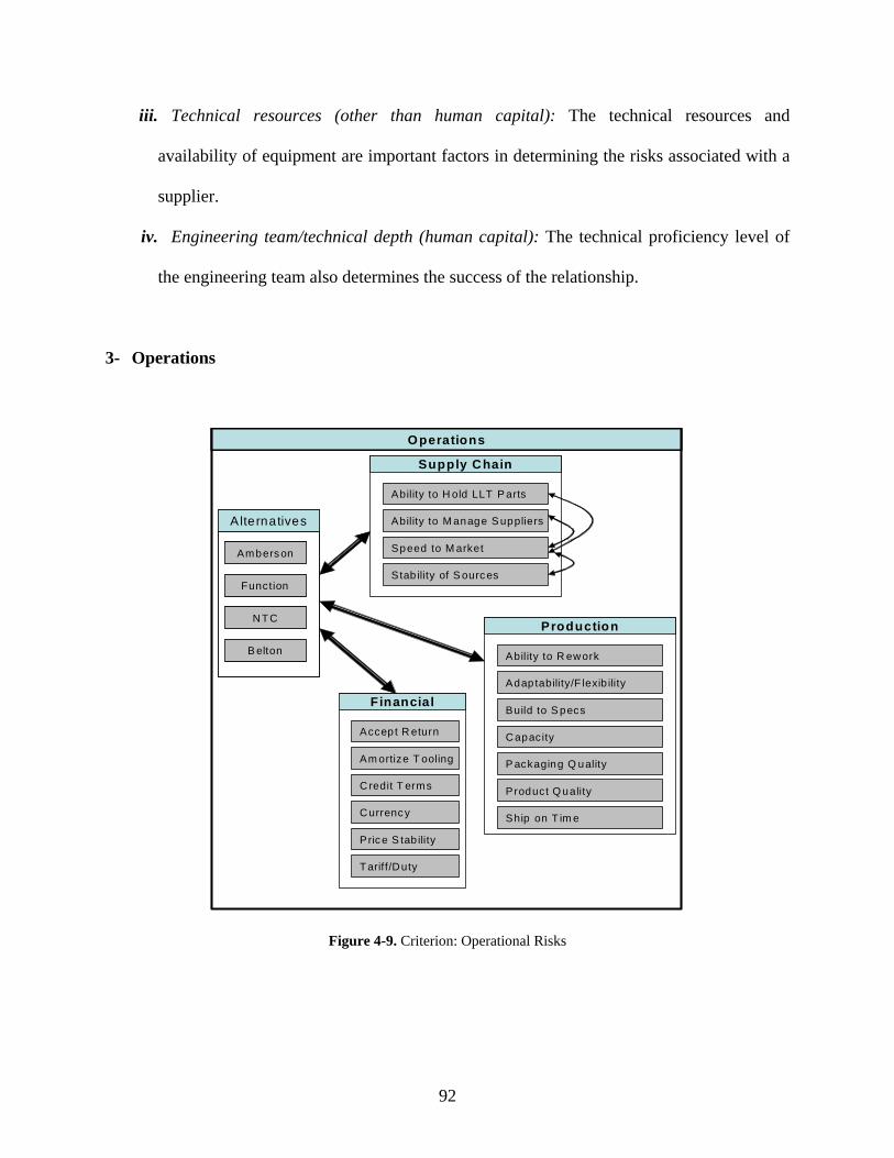
92
iii. Technical resources (other than human capital): The technical resources and
availability of equipment are important factors in determining the risks associated with a
supplier.
iv. Engineering team/technical depth (human capital): The technical proficiency level of
the engineering team also determines the success of the relationship.
3- Operations
Operations
Ambers on
Function
NTC
B elton
Alternatives
Ambers on
Function
NTC
B elton
Alternatives
Ability to H old LLT P arts
Ability to M anage S uppliers
Supply Chain
Stab ility of S ourc es
Speed to M arket
Ability to R ework
Adaptability/F lexib ility
Production
C apacity
Build to S pecs
P ackaging Q uality
Product Q uality
Ship on T im e
Accept R eturn
Am ortize T ooling
Financial
Currenc y
Credit T erms
Pric e S tab ility
Tariff/Duty
Figure 4-9. Criterion: Operational Risks
93
a) Financial
i. Price stability: If the supplier tends to increase prices, or as the economies of scale are
achieved the supplier is not willing to lower the prices, the financial risks are higher.
ii. Tariff/Duty: The tariff and duty restrictions may exist for some regions for particular
products. Moreover, the duty rates and taxes may change in some countries. By looking
at the historical trends and the economic indicators, the risks associated with the location
can be predicted.
iii. Currency: The potency of fluctuating currencies will elevate the risk factors. There is
no currency related risk currently, but the criterion is included for future problems.
iv. Credit Terms: The supplier’s attitude toward the credit term agreement is a factor in
financial risks.
v. Acceptance of returns: Once the product is in the market, product returns will occur due
to defects and other miscellaneous reasons. Risks are lower if a supplier is willing to
accept returns.
vi. Amortization of tooling: The way the supplier calculates the costs is important. For
instance, the tooling amortization may be reflected on the future prices, in which case
SIMA will be paying extra money.
b) Production
i. Quality: The level of product quality that the supplier offers may be predicted by
evaluating the existing or previous products. Poor quality is always a big risk in the U.S.
market.

94
ii. On time shipment: In a market environment with very short life cycles it is important to
work with a supplier that can ship products on time without any delays.
iii. Building to specifications: A supplier that does not manufacture products according to
the exact design specifications creates the risk of losing market share due to
unsatisfactory product features.
iv. Adaptability/ Flexibility: A supplier who has the technical capability and resources to
adapt to last minute changes in design and/or product timeline mitigates the risks
considerably.
v. Packaging quality: The packaging quality is an important factor for a product to be
successful in the market.
vi. Capacity: The sufficiency of the supplier’s maximum capacity for the forecasted
demand.
vii. Ability to rework: A supplier needs to be able to rework returned products.
c) Supply Chain
i. Speed to market: It is essential that the product is launched on time. New and
innovative products are usually launched before Christmas in order to benefit from
consumption boost in that period. Moreover, if a product’s launch is late, the risk of
having a competitor launching the same product is higher.
ii. Stability of sources (their sources): The stability of a supplier’s sources for raw
material and energy is important to ensure the continuity of production.
iii. Ability to manage suppliers (their own): A supplier should be able to manage its own
suppliers to eliminate unexpected delays.
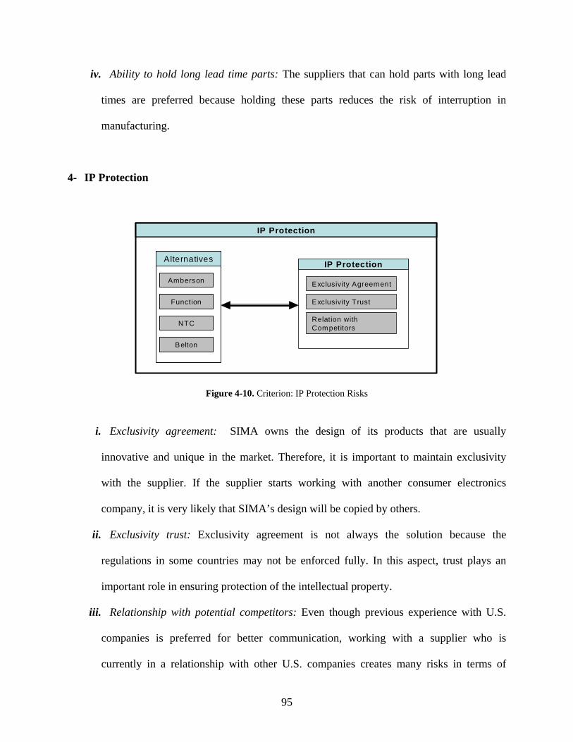
95
iv. Ability to hold long lead time parts: The suppliers that can hold parts with long lead
times are preferred because holding these parts reduces the risk of interruption in
manufacturing.
4- IP Protection
IP Protection
Amberson
Function
NTC
Belton
Alternatives
Amberson
Function
NTC
Belton
Alternatives
Exclusivity Agreement
Exclusivity Trust
IP Protection
Relation with Competitors
Figure 4-10. Criterion: IP Protection Risks
i. Exclusivity agreement: SIMA owns the design of its products that are usually
innovative and unique in the market. Therefore, it is important to maintain exclusivity
with the supplier. If the supplier starts working with another consumer electronics
company, it is very likely that SIMA’s design will be copied by others.
ii. Exclusivity trust: Exclusivity agreement is not always the solution because the
regulations in some countries may not be enforced fully. In this aspect, trust plays an
important role in ensuring protection of the intellectual property.
iii. Relationship with potential competitors: Even though previous experience with U.S.
companies is preferred for better communication, working with a supplier who is
currently in a relationship with other U.S. companies creates many risks in terms of
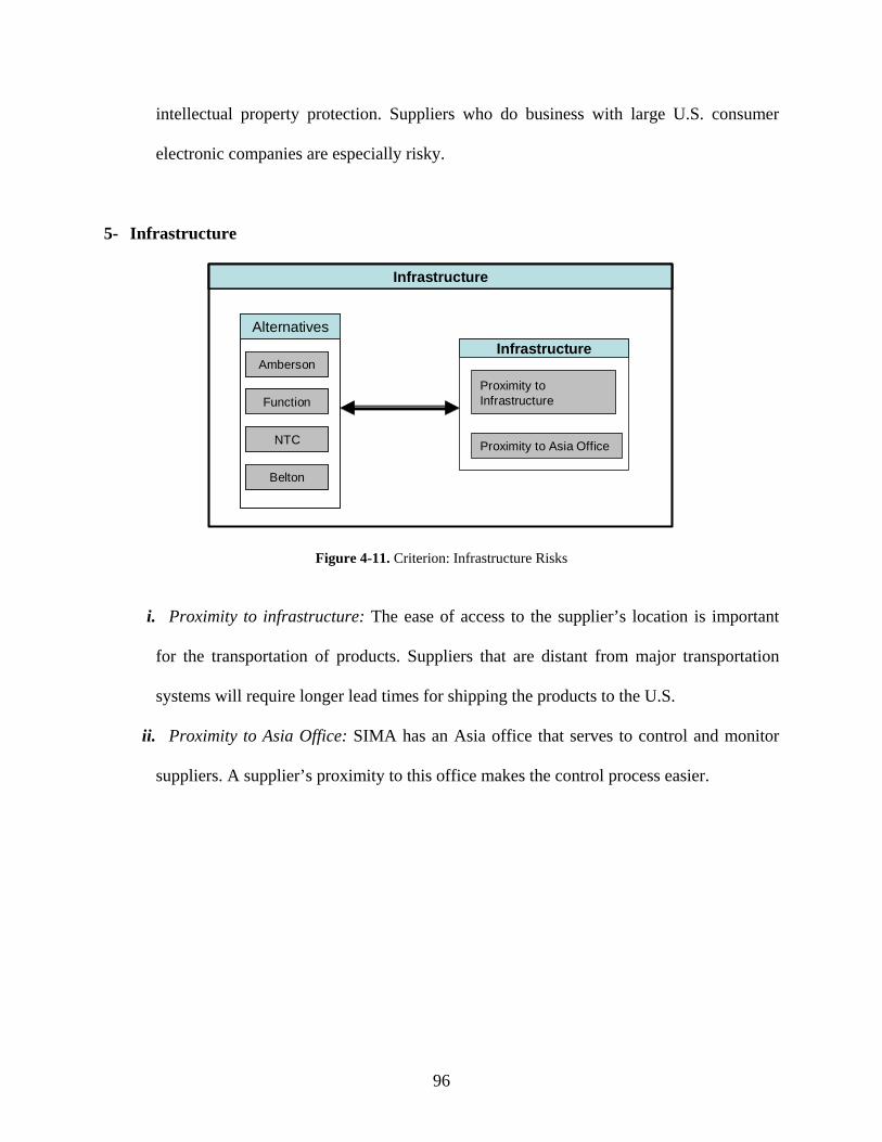
96
intellectual property protection. Suppliers who do business with large U.S. consumer
electronic companies are especially risky.
5- Infrastructure
Infrastructure
Amberson
Function
NTC
Belton
Alternatives
Amberson
Function
NTC
Belton
Alternatives
Proximity toInfrastructure
Infrastructure
Proximity to Asia Office
Figure 4-11. Criterion: Infrastructure Risks
i. Proximity to infrastructure: The ease of access to the supplier’s location is important
for the transportation of products. Suppliers that are distant from major transportation
systems will require longer lead times for shipping the products to the U.S.
ii. Proximity to Asia Office: SIMA has an Asia office that serves to control and monitor
suppliers. A supplier’s proximity to this office makes the control process easier.
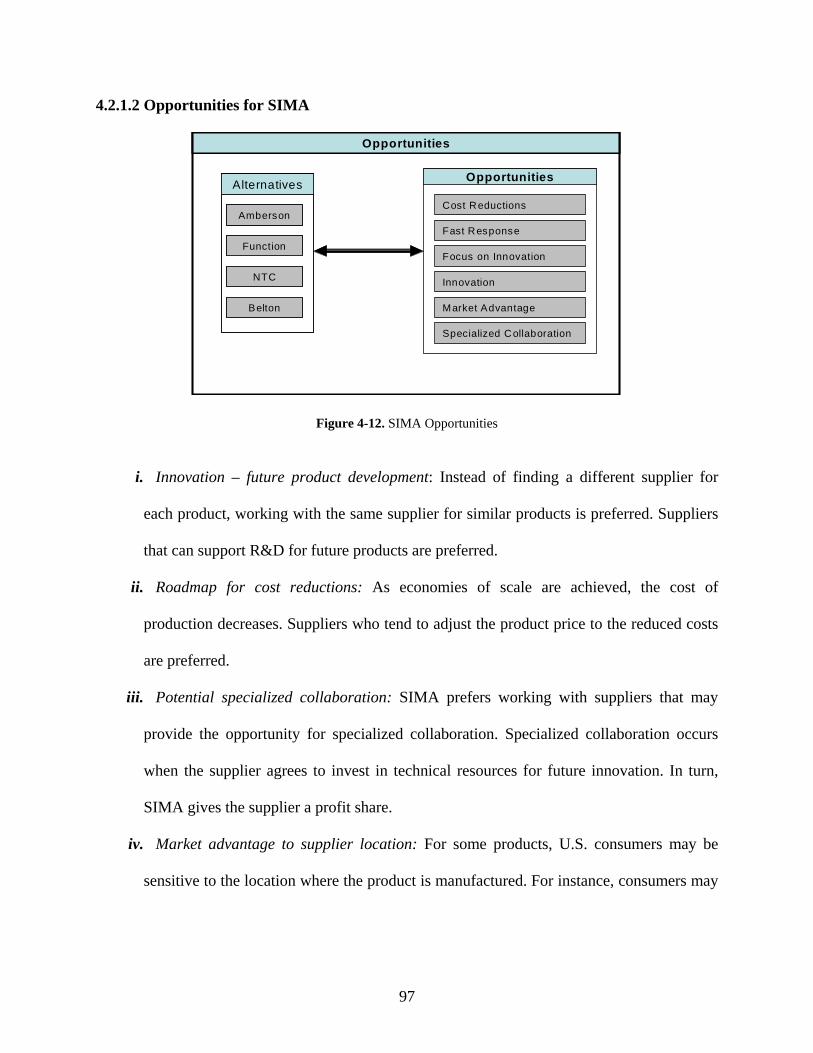
97
4.2.1.2 Opportunities for SIMA
Opportunities
Amberson
Function
NTC
Belton
Alternatives
Amberson
Function
NTC
Belton
Alternatives
Cost Reductions
Fast Response
Opportunities
Innovation
Focus on Innovation
Market Advantage
Specialized Collaboration
Figure 4-12. SIMA Opportunities
i. Innovation – future product development: Instead of finding a different supplier for
each product, working with the same supplier for similar products is preferred. Suppliers
that can support R&D for future products are preferred.
ii. Roadmap for cost reductions: As economies of scale are achieved, the cost of
production decreases. Suppliers who tend to adjust the product price to the reduced costs
are preferred.
iii. Potential specialized collaboration: SIMA prefers working with suppliers that may
provide the opportunity for specialized collaboration. Specialized collaboration occurs
when the supplier agrees to invest in technical resources for future innovation. In turn,
SIMA gives the supplier a profit share.
iv. Market advantage to supplier location: For some products, U.S. consumers may be
sensitive to the location where the product is manufactured. For instance, consumers may
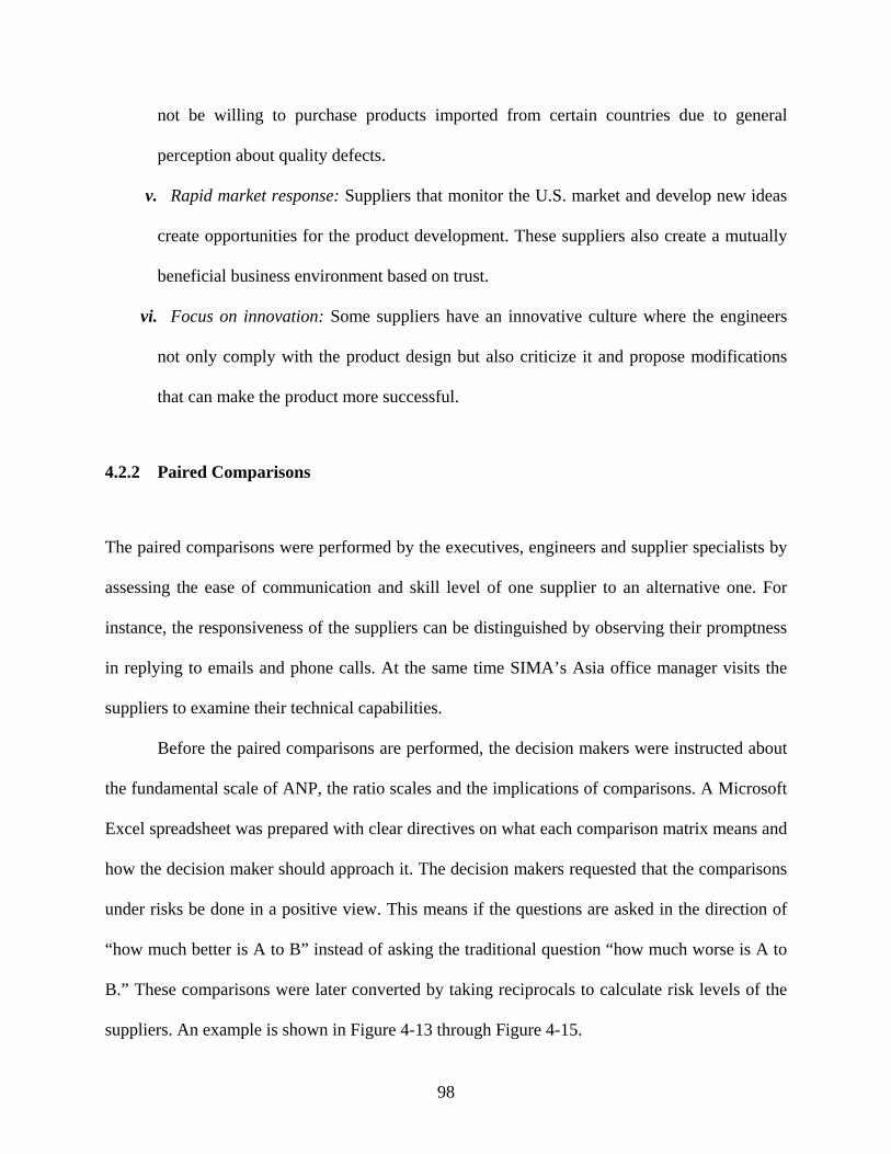
98
not be willing to purchase products imported from certain countries due to general
perception about quality defects.
v. Rapid market response: Suppliers that monitor the U.S. market and develop new ideas
create opportunities for the product development. These suppliers also create a mutually
beneficial business environment based on trust.
vi. Focus on innovation: Some suppliers have an innovative culture where the engineers
not only comply with the product design but also criticize it and propose modifications
that can make the product more successful.
4.2.2 Paired Comparisons
The paired comparisons were performed by the executives, engineers and supplier specialists by
assessing the ease of communication and skill level of one supplier to an alternative one. For
instance, the responsiveness of the suppliers can be distinguished by observing their promptness
in replying to emails and phone calls. At the same time SIMA’s Asia office manager visits the
suppliers to examine their technical capabilities.
Before the paired comparisons are performed, the decision makers were instructed about
the fundamental scale of ANP, the ratio scales and the implications of comparisons. A Microsoft
Excel spreadsheet was prepared with clear directives on what each comparison matrix means and
how the decision maker should approach it. The decision makers requested that the comparisons
under risks be done in a positive view. This means if the questions are asked in the direction of
“how much better is A to B” instead of asking the traditional question “how much worse is A to
B.” These comparisons were later converted by taking reciprocals to calculate risk levels of the
suppliers. An example is shown in Figure 4-13 through Figure 4-15.
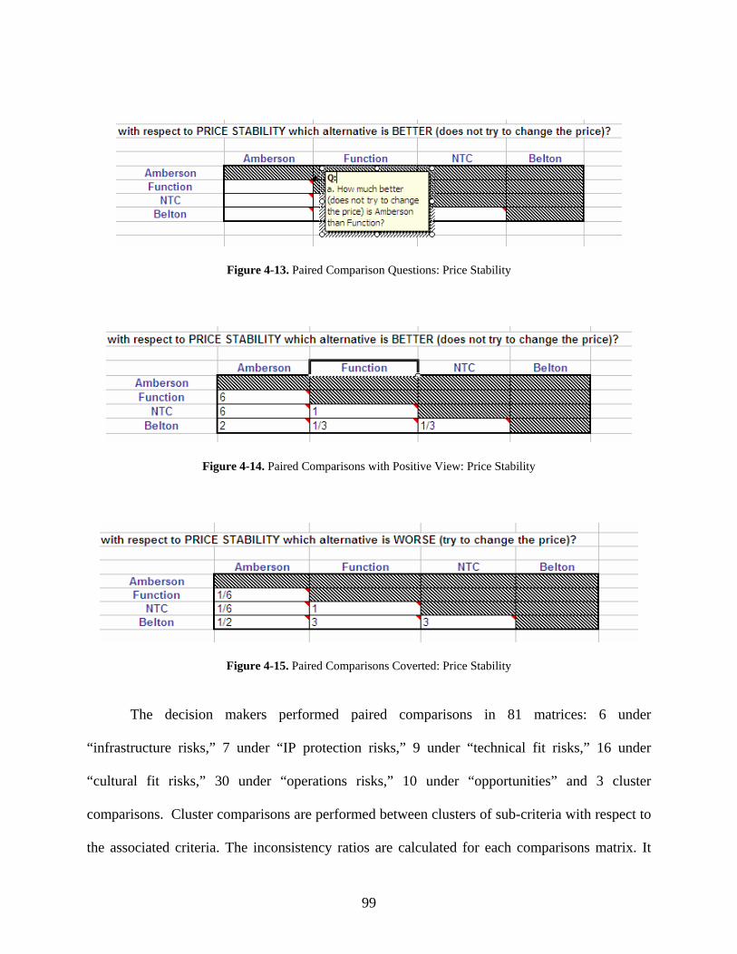
99
Figure 4-13. Paired Comparison Questions: Price Stability
Figure 4-14. Paired Comparisons with Positive View: Price Stability
Figure 4-15. Paired Comparisons Coverted: Price Stability
The decision makers performed paired comparisons in 81 matrices: 6 under
“infrastructure risks,” 7 under “IP protection risks,” 9 under “technical fit risks,” 16 under
“cultural fit risks,” 30 under “operations risks,” 10 under “opportunities” and 3 cluster
comparisons. Cluster comparisons are performed between clusters of sub-criteria with respect to
the associated criteria. The inconsistency ratios are calculated for each comparisons matrix. It
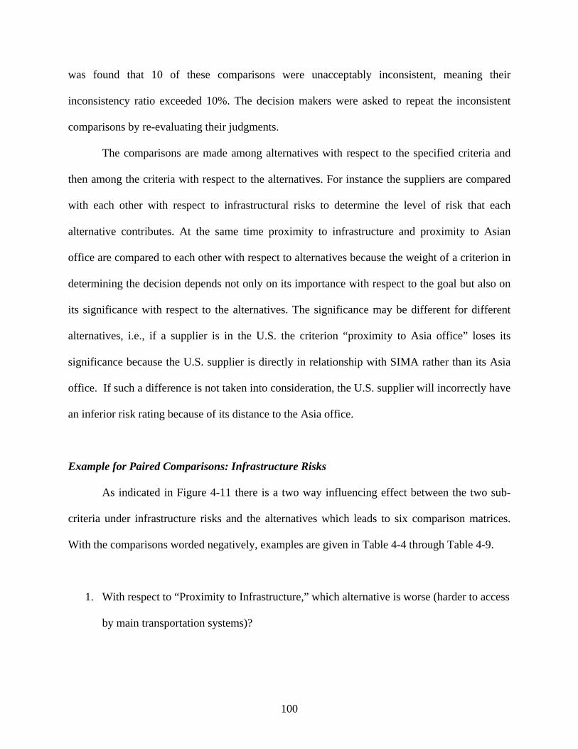
100
was found that 10 of these comparisons were unacceptably inconsistent, meaning their
inconsistency ratio exceeded 10%. The decision makers were asked to repeat the inconsistent
comparisons by re-evaluating their judgments.
The comparisons are made among alternatives with respect to the specified criteria and
then among the criteria with respect to the alternatives. For instance the suppliers are compared
with each other with respect to infrastructural risks to determine the level of risk that each
alternative contributes. At the same time proximity to infrastructure and proximity to Asian
office are compared to each other with respect to alternatives because the weight of a criterion in
determining the decision depends not only on its importance with respect to the goal but also on
its significance with respect to the alternatives. The significance may be different for different
alternatives, i.e., if a supplier is in the U.S. the criterion “proximity to Asia office” loses its
significance because the U.S. supplier is directly in relationship with SIMA rather than its Asia
office. If such a difference is not taken into consideration, the U.S. supplier will incorrectly have
an inferior risk rating because of its distance to the Asia office.
Example for Paired Comparisons: Infrastructure Risks
As indicated in Figure 4-11 there is a two way influencing effect between the two sub-
criteria under infrastructure risks and the alternatives which leads to six comparison matrices.
With the comparisons worded negatively, examples are given in Table 4-4 through Table 4-9.
1. With respect to “Proximity to Infrastructure,” which alternative is worse (harder to access
by main transportation systems)?

101
Table 4-4. Paired Comparisons: Proximity to Infrastructure
Consistency Ratio: 0.080
2. With respect to “Proximity to Asia Office,” which alternative is worse (harder to access)?
Table 4-5. Paired Comparisons: Proximity to Asia Office
Amberson Function NTC Belton Amberson Function 1/8
NTC 1 6 Belton 1 6 1
Consistency Ratio: 0.002
3. With respect to “Amberson” which criterion is more important?
Table 4-6. Paired Comparisons: Infrastructure Risks w.r.t. Amberson
Prox. Infrastructure Prox. Asia Office Prox. Infrastructure Prox. Asia Office 1
Consistency Ratio: 0
4. With respect to “Function” which criterion is more important?
Table 4-7. Paired Comparisons: Infrastructure Risks w.r.t. Function
Prox. Infrastructure Prox. Asia Office Prox. Infrastructure Prox. Asia Office 1/6
Consistency Ratio: 0
Amberson Function NTC Belton Amberson Function 1
NTC 1/6 1/3 Belton 1/3 1 1
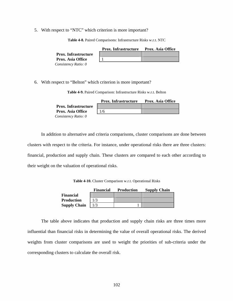
102
5. With respect to “NTC” which criterion is more important?
Table 4-8. Paired Comparisons: Infrastructure Risks w.r.t. NTC
Prox. Infrastructure Prox. Asia Office Prox. Infrastructure Prox. Asia Office 1
Consistency Ratio: 0
6. With respect to “Belton” which criterion is more important?
Table 4-9. Paired Comparison: Infrastructure Risks w.r.t. Belton
Prox. Infrastructure Prox. Asia Office Prox. Infrastructure Prox. Asia Office 1/6
Consistency Ratio: 0
In addition to alternative and criteria comparisons, cluster comparisons are done between
clusters with respect to the criteria. For instance, under operational risks there are three clusters:
financial, production and supply chain. These clusters are compared to each other according to
their weight on the valuation of operational risks.
Table 4-10. Cluster Comparison w.r.t. Operational Risks
Financial Production Supply Chain Financial Production 1/3 Supply Chain 1/3 1
The table above indicates that production and supply chain risks are three times more
influential than financial risks in determining the value of overall operational risks. The derived
weights from cluster comparisons are used to weight the priorities of sub-criteria under the
corresponding clusters to calculate the overall risk.

103
4.2.3 Synthesis
First, for each comparison matrix the priorities are calculated by taking the eigenvectors.
Table 4-11. Infrastructure Risks Priority Calculation
Amberson Function NTC Belton Eigenvector Amberson 1 1 6 3 0.1047 Function 1 1 3 1 0.1675
NTC 1/6 1/3 1 1 0.4409 Belton 1/3 1 1 1 0.2869
Later, under each cluster a stochastic supermatrix is formed where columns are the
priorities associated with all of the comparison matrices under that cluster. In the supermatrix
the cells that do not represent any influence are assigned zero. The limiting power of the
supermatrix is a stabilized matrix with identical columns where elements are the priorities of the
alternatives with respect to the cluster criteria. The supermatrix of infrastructure risks is shown
in Table 4-12 as an example.
Table 4-12. Supermatrix: Infrastructure Risks
Cluster Alternatives Infrastructure Infrastructure Risks Amberson Function NTC Belton Prox.Infra. Prox.Asia
Amberson 0 0 0 0 0.1047 0.0993Function 0 0 0 0 0.1675 0.6879NTC 0 0 0 0 0.4409 0.1064
Alternatives
Belton 0 0 0 0 0.2869 0.1064Infrastructure Prox.Infra. 0.5 0.143 0.5 0.143 0 0 Prox.Asia 0.5 0.857 0.5 0.857 0 0
These priorities are multiplied by the associated cluster weights obtained from the paired
cluster comparisons. The weighted sum in normalized form gives the overall risk and
opportunity priorities of the alternatives. Table 4-13 shows how the values of risks corresponding
to alternatives are calculated.
104
Table 4-13. Calculations for Risk Priorities
Cultural Fit Technical Fit Operations Control Criterion CC limiting CC 0.11466 limiting CC 0.40406 limiting CC 0.19826Normalized 0.11466 0.40406 0.19826
Alternatives Idealized
(CC x Ideal.
) Idealized (CC x
Ideal.) Idealized (CC x
Ideal.)Amberson 0.4399 0.0504 0.0923 0.0373 0.2034 0.0403Function 0.6309 0.0723 0.3118 0.1260 0.6410 0.1271NTC 1.0000 0.1147 1.0000 0.4041 1.0000 0.1983Belton 0.3122 0.0358 0.2739 0.1107 0.2250 0.0446 IP Protection Infrastructure Control Criterion CC
limiting CC 0.21483 limiting CC
0.06819
Normalized 0.21483 0.06819
Alternatives Idealized (CC x
Ideal.) Idealized (CC x
Ideal.) SUM Normal
izedAmberson 0.3067 0.0659 0.1797 0.0123 0.2062 0.1121Function 1.0000 0.2148 1.0000 0.0682 0.6084 0.3308NTC 0.2534 0.0544 0.3372 0.0230 0.7944 0.4319Belton 0.0964 0.0207 0.2695 0.0184 0.2302 0.1251
The opportunity merit is formed of only one cluster, therefore the priorities calculated
from the limiting supermatrix are directly the opportunity priorities of the respective alternatives.
The limiting supermatrix’s columns corresponding with the alternatives are:
• Amberson: 0.24442 Normalized: 0.4888
• Function: 0.07983 Normalized: 0.1597
• NTC: 0.03975 Normalized: 0.0795
• Belton: 0.13599 Normalized: 0.2720
Employing the mathematical notations, the risk and opportunity weights can be expressed as:
1R = 0.1121 2R = 0.3308 3R = 0.4319 4R = 0.1251
1O = 0.4888 2O = 0.1597 3O = 0.0795 4O = 0.2720
105
4.3 INTEGRATED MODEL FOR SIMA CORPORATION
There are three objectives: minimizing total costs, minimizing total risks and maximizing total
opportunities. Minimization of the total cost is modeled and illustrated in Section 4.1. The other
objectives are based on intangible values and can be defined by making use of the results of the
ANP model. For SIMA, risks arise mainly due to the risk of losing the intellectual property
(design of product). Difficulties in communication and management also play an important role
in determining the level of risk. These types of managerial and IP risks are nondiversifiable
because the existence of multiple suppliers means the probability of having a competitor copying
the design and incurring communication problems increases. Thus, it is reasonable to assume
that total risk of the decision is defined by is the sum of the risks associated with each selected
supplier and the objective “minimization of total risks” can be denoted as:
π2(x) = ( )∑∈Ii
iibRmin .
In general, SIMA perceives opportunity as the potential for working with the same
supplier for innovative modifications to the same product and for development of future
products. In an interview the CEO of SIMA clearly stated “It is always better to work with
suppliers that we have dealt with before. Especially anything that is a new technology; i.e., a new
product from ground up should be developed with a long term supplier.” Based on this
perception it is reasonable to assume that working with different suppliers increases the chances
for building trustworthy relationships for future products. Therefore, the opportunities can be
classified as diversifiable, meaning that the total opportunity is defined as the sum of individual
opportunities of the selected suppliers. The objective of maximizing total opportunity can be
denoted as:
106
π3(x) = ( )∑∈Ii
iibOmax .
Since the total risks and opportunities are defined as the sum of individual risk and
opportunity values the direction of optimality is easy to foresee. No matter what the demand is,
maximization of total opportunities requires working with as many suppliers as possible, while
minimization of total risks requires choosing only that one supplier with the minimum associated
risk.
The ranking of risks (from least to most risky) and opportunities (from most to least
opportunistic) is the same: Amberson, Belton, Function and NTC. In order to minimize total
risks, only Amberson should to be chosen as the outsourcing supplier. However if demand does
not exceed 5,000 units, some part of production needs to be outsourced to Belton because
Amberson’s minimum order quantity requirement is not fulfilled for some product types. Since
diversifying to two suppliers is much riskier, in order minimize the total risk Belton is selected
for manufacturing of all of the products. If the total demand exceeds 5,000, then the minimum
order quantity restrictions are not binding and all of manufacturing is outsourced to Amberson.
In order to maximize total opportunities, supplier selection should be as diverse as
possible which leads to distribution of production as much as possible subject to meeting
minimum order quantities. If demand is less than 5,000, the minimum order quantities of
Amberson, NTC and Belton can be satisfied thus the opportunity objective is maximized by
distributing production to these three suppliers. Once demand exceeds 5,000 all of the supplier
minimum order quantities can be satisfied and maximum opportunity is achieved by selecting all
four of the suppliers. Obviously, selecting multiple suppliers results in considerable cost and risk
growth.

107
The multi-objective problem is solved by utilizing the epsilon-constraint multi-objective
optimization method with Pareto maximum bounds. For solving the opportunity objective, a set
of constraints needs to be added in order to ensure that binary variable associated with selection
of the supplier is 0 if there is no production. The set of constraints is:
iiPp
ip bmox ≥∑∈
∀ Ii ∈ (4-9)
Considering the breakeven points for cost, risk and opportunity objectives, the tradeoff
analysis is performed in three segments:
1. Demand between 2,500 and 5,000;
2. Demand between 5,000 and 8,873; and
3. Demand more than 8,873.
Since the ranking of supplier alternatives in terms of opportunities, risks and costs does
not change within the segments, the solution set (selected suppliers) is the same independent of
the demand within each segment. Figure 4-16 through Figure 4-18 depict the Pareto optimal
points for selected demand volumes. These Pareto optimal points illustrate the best supplier
selections and the tradeoffs between objectives. The tradeoffs between objectives may be
evaluated by the decision maker within the framework of the company’s goals and competitive
advantages.
1- Demand between 2,500 and 5,000 units
To illustrate tradeoff characteristics in this region the multi-objective problem is solved
for a demand of 4,600 units and the results are presented in Figure 4-16.

108
RiskRisk
Opportunity
Opportunity
Cos
tC
ost
POINT BPOINT B
POINT CPOINT C
POINT APOINT A
*Min Cost
*Max Opp
*Min Risk
Cost: $220,966Risk: 0.1251Opp.: 0.272Suppliers: Belton
Cost: $216,790Risk: 0.2372Opp.: 0.7608Suppliers: Belton, Amberson
Cost: $295,930Risk: 0.6691Opp.: 0.8403Suppliers: Belton, Amberson,NTC
Figure 4-16. Pareto Front Points for Demand = 4,600 units
The Pareto points are the utopia points for two reasons. First, the minimum order quantity
limits the number of combinations for supplier selection. Second, the total risk and opportunity
values can take on distinct values because they are defined as the sum of individual risk and
opportunity values.
At point “A” maximum opportunity is achieved by working with three different suppliers
however the costs and risks elevate drastically at rates of 37% and 400% respectively. Therefore,
unless opportunity is a very important priority, it is not reasonable to select decision point “A.”
Minimum cost is ensured at point “C” by selecting Belton and Amberson and distributing the
production by minimizing the cost objective. Furthermore, by slightly letting the total cost
increase approximately 2%, the total risk of business can be decreased by approximately 50%
while the total opportunity decreases by approximately 65% at point “B.” Since by sacrificing a
little from cost objective considerably reduces risks and increases opportunities, such a sacrifice

109
is reasonable to make. Therefore, the decision points “B” and “C’ are credible alternatives. The
final decision of choosing whether to outsource to only Belton or to both Belton and Amberson
may be made by assessing the company’s values, past experience and the decision maker’s
opinions.
A more theoretical approach is to elicitate utility functions associated with each
objective. Utility is defined as a measure of happiness (preference) represented on a scale of 0 to
1 where 1 represents the maximum preference and 0 represents the minimum preference. An
efficient method to elicitate utility functions is the certainty equivalent method which finds the
utilities by asking the decision maker his/her preferences in situations where binary choices are
presented between a sure amount and a simple gamble [100]. For instance in this case, in order
to elicit the utility function for “cost” a decision maker is asked to pick the best option in
consequent situations such as “choosing between a sure amount of cost $250,000 in total cost to
a 50-50 chance of incurring a cost of either $200,000 or $300,000. As a result, the utility
functions associated with each objective are derived representing the amount of utility (between
0 and 1) for the objective values. The utilities for the alternatives are calculated by adding the
utility for the corresponding objective values and the final decision is made by choosing the
alternative which gives the maximum total utility.
2- Demand between 5,000 and 8,873 units
To illustrate tradeoff characteristics in this region the multi-objective problem is solved
for a demand of 7,000 units and the results are shown in Figure 4-17.
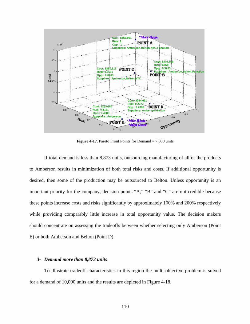
110
POINT APOINT A
POINT BPOINT BPOINT CPOINT C
POINT DPOINT D
POINT EPOINT E
Cost: $466,051Risk: 1Opp.: 1Suppliers: Amberson,Belton,NTC,Function
Cost: $376,659Risk: 0.568Opp.: 0.9205Suppliers: Amberson,Belton,Function
Cost: $367,211Risk: 0.6691Opp.: 0.8403Suppliers: Amberson,Belton,NTC
Cost: $284,631Risk: 0.2372Opp.: 0.7608Suppliers: Amberson,Belton
Cost: $263,865Risk: 0.1121Opp.: 0.4888Suppliers: Amberson
*Min Risk*Min Cost
*Max Opp.
RiskRisk
Opportunity
Opportunity
Cos
tC
ost
Figure 4-17. Pareto Front Points for Demand = 7,000 units
If total demand is less than 8,873 units, outsourcing manufacturing of all of the products
to Amberson results in minimization of both total risks and costs. If additional opportunity is
desired, then some of the production may be outsourced to Belton. Unless opportunity is an
important priority for the company, decision points “A,” “B” and “C” are not credible because
these points increase costs and risks significantly by approximately 100% and 200% respectively
while providing comparably little increase in total opportunity value. The decision makers
should concentrate on assessing the tradeoffs between whether selecting only Amberson (Point
E) or both Amberson and Belton (Point D).
3- Demand more than 8,873 units
To illustrate tradeoff characteristics in this region the multi-objective problem is solved
for a demand of 10,000 units and the results are depicted in Figure 4-18.
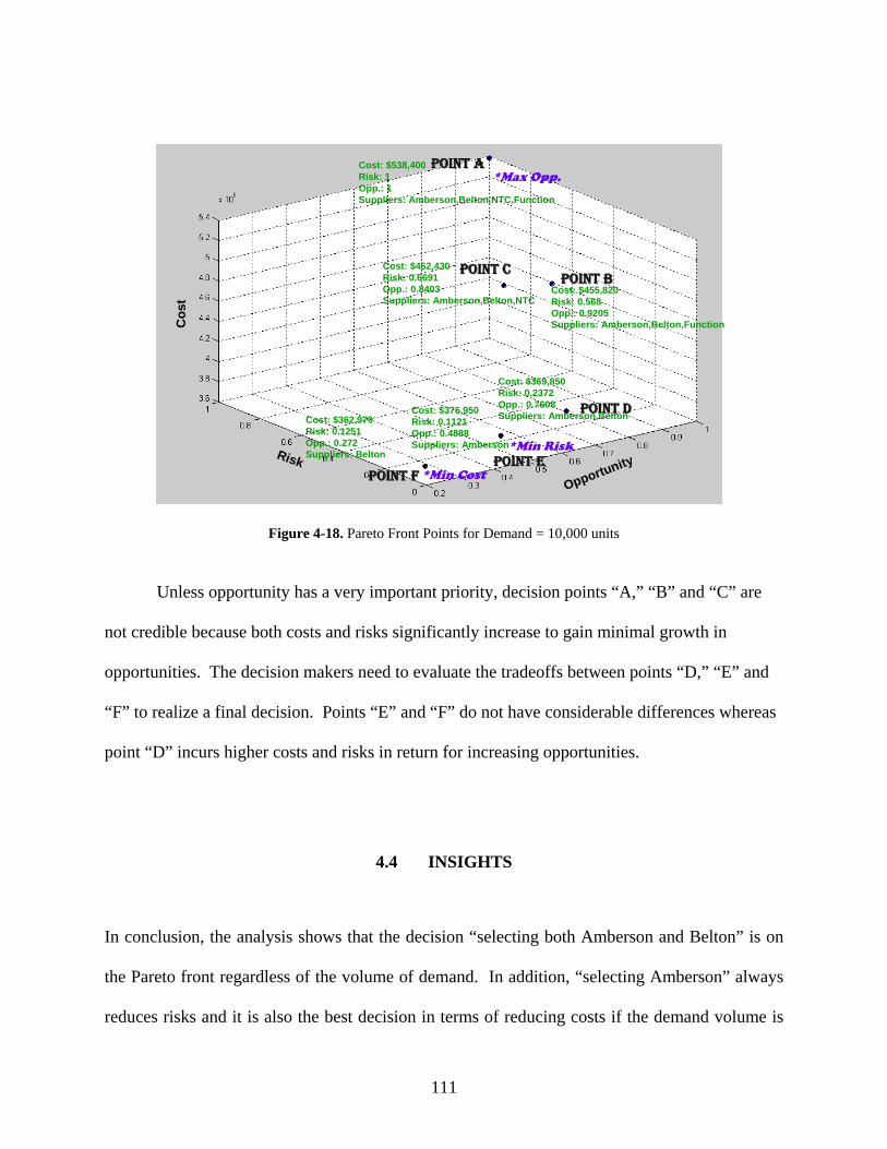
111
POINT APOINT A
POINT BPOINT BPOINT CPOINT C
POINT DPOINT D
POINT EPOINT EPOINT FPOINT F
RiskRisk
Opportunity
Opportunity
Cos
tC
ost
Cost: $538,400Risk: 1Opp.: 1Suppliers: Amberson,Belton,NTC,Function
Cost: $455,820Risk: 0.568Opp.: 0.9205Suppliers: Amberson,Belton,Function
Cost: $452,430Risk: 0.6691Opp.: 0.8403Suppliers: Amberson,Belton,NTC
Cost: $369,850Risk: 0.2372Opp.: 0.7608Suppliers: Amberson,BeltonCost: $376,950
Risk: 0.1121Opp.: 0.4888Suppliers: Amberson
Cost: $362,970Risk: 0.1251Opp.: 0.272Suppliers: Belton
*Min Cost
*Min Risk
*Max Opp.
Figure 4-18. Pareto Front Points for Demand = 10,000 units
Unless opportunity has a very important priority, decision points “A,” “B” and “C” are
not credible because both costs and risks significantly increase to gain minimal growth in
opportunities. The decision makers need to evaluate the tradeoffs between points “D,” “E” and
“F” to realize a final decision. Points “E” and “F” do not have considerable differences whereas
point “D” incurs higher costs and risks in return for increasing opportunities.
4.4 INSIGHTS
In conclusion, the analysis shows that the decision “selecting both Amberson and Belton” is on
the Pareto front regardless of the volume of demand. In addition, “selecting Amberson” always
reduces risks and it is also the best decision in terms of reducing costs if the demand volume is

112
low. On the other hand, “selecting Belton” does not increase risks considerably while offering
the lowest total cost if the demand volume is high. One recommendation is for SIMA to
outsource to Amberson if demand is low and then start shifting production to Belton as demand
increases. The final decision depends on SIMA’s corporate values and the decision makers’
perspectives and experience.
This empirical study leads to broader insights on the process of offshore outsourcing
decisions and the value of employing an integrated decision model that can incorporate tangible
and intangible values. As a result,
• A comprehensive analysis shows that some of the supplier alternatives can be eliminated
from consideration. In this case, NTC and Function are eliminated from the decision
space regardless of the demand volume. Reducing the number of alternatives that have to
be dealt with ensures both a less complex and a more accurate decision process.
• By exploiting the variations in the optimal decision as the parameters change, a decision
can be made based on the product’s entire life cycle rather than solely on the present
values. This allows the company to establish a strategic action plan which may be
executed according to the changing business conditions. For instance, SIMA’s action
plan may be to outsource to Amberson with a contractual agreement that can allow
production to shift to Belton as the product goes through later product life phases.
Another action plan may be to negotiate with Amberson so that it can maintain its
advantageous status by lowering product prices towards the maturity and declining
phases of the product.
• The integrated decision model developed incorporates both tangible and intangible
variables and gives multiple optimal decisions while presenting the tradeoffs between
113
these decision points. These results not only provide answers for the company but also
can be used as a basis of negotiation with the suppliers during offshore outsourcing
relations. If negotiations are only based on costs, a win-win situation cannot be achieved
because changing the unit price favors one side while hurting the other side. Instead,
other variables such as operational and managerial considerations may be included in the
negotiation process to achieve a win-win situation. The results of this analysis explicitly
demonstrate this argument both to the suppliers and to SIMA.

114
5.0 CAPTIVE OFFSHORING EMPIRICAL STUDY: XYZ
The second empirical study is also based on a real case for a global corporation that requested
confidentiality. Hence, the company is referred by the name “XYZ” and the product is referred
as a “perishable food product” without giving the actual names. XYZ is a global U.S.-based
company that produces and markets perishable food items in different regions of the world. Over
the years, the company’s international setting has allowed the operations to expand and diversify
in terms of both volume and quality. Recently, the consequences of globalization began to put
extra pressure on the market competition, forcing the company executives to seriously consider
transferring some of its operations overseas. At the present time, the production for the North
American consumer market takes place in the U.S. by utilizing the latest technologies in
agriculture and processing. However due to the increasing cost of labor and transportation, and
pressure from the market to hold prices steady, the company has given serious thought to cost
reduction strategies. Offshoring became an attractive option for management to maintain the
company’s market share by transferring a part of the manufacturing facility offshore with
contractual agreements supported by regional investments.
Offshoring from the U.S. is being considered for the front-end portion of the production
process where the raw materials are converted to a semi-finished product. The process that is in
consideration for outsourcing is divided into two parts: Raw Food Production (RFP) and Semi-

115
finished Food Production (SFP). Figure 5-1 depicts a representation of the front end process that
is in consideration for offshoring.
Raw Material
Proc. A1
Proc. A2
Proc.A3
Proc. A4
Raw
Product
Proc.B1
Proc. B2
Proc. B3
SemifinishedProduct
Raw Food Production (RFP)
Semi-finished Food Production (SFP)
Proc.C1
Proc. C2
Proc. C3
Proc. C4
End Product
End Food Process
Figure 5-1. Representative Process Flow - XYZ
There are four alternative offshore locations (whose names are not disclosed to maintain
confidentiality). The countries are referred with the regional names; remaining in-house in the
U.S. is also included as an alternative to incorporate the decision of whether or not to outsource.
The alternatives are:
1. Outsource the process to an Asian location
2. Outsource the process to a Middle Eastern location
3. Outsource the processes to an Eastern European location
4. Outsource the process to a South American location
5. Remain in the U.S.
Since the quality of a perishable food product is important, offshore outsourcing with a
subcontractor is not an option. Instead, investment will be made (possibly with a third party
venture) in the region and the semi-finished product processed at the destination will be directly
imported to facilities in the U.S. and Western Europe where the product will be further processed
and sold under the company’s brand name.
116
5.1 COST ANALYSIS
Cost of production plays a major role in assessing alternatives for offshoring. In most of the
global supplier and location selection cases, costs are evaluated on the basis of price quotes that
are typically provided by vendors. This technique may be fairly accurate for consumer items
whose production will not require a capital investment. However, it is not recommended for long
term offshoring practices that require considerable investment because the analyses based on
these values, may be biased not only due to the vendor’s willingness to increase profit margins,
but also because of the possibility that the computational tools that the vendor uses in the
calculation of product costs may not be sufficiently accurate enough. Most vendors would prefer
escalating the depreciation rates, thereby augmenting the overhead, which will result in an over-
estimation of product costs. As in the case of XYZ, the offshoring process may not be done
through a contractual agreement and in such cases it is not correct to base the decision on vendor
quotes, as these quotes may be for lower quality products and may not reflect the real costs that
will be incurred. A more dependable and consistent way for cost assessment is analyzing the
alternatives by calculating the associated product costs through a set of tools based on the actual
core parameters, such as labor wages and inflation rates that can be obtained from objective data
sources. From this standpoint, Activity Based Costing (ABC) is a valuable methodology that can
appropriately be utilized for an unbiased offshoring decision.
5.1.1 The Activity Based Costing Technique
Product costs can be divided into two major groups: direct and indirect costs. Direct labor (DL)
and direct material (DM) costs are considered to be the direct costs, i.e., costs that can be traced
117
directly to the product or process. The remaining costs are grouped as indirect costs such as
overhead (OH) costs, making them difficult to trace to the products or processes. It is the
significant increase of automation in the manufacturing process (and subsequently the reduction
in direct labor) that has led to recognition of the importance of OH costs. Prior methods to
allocate OH to products and processes were based on a particular volume-based metric such as
DL content and became inappropriate in this new highly automated manufacturing environment.
ABC which was first defined by Burns and Kaplan in 1987 [101] is an alternative method for
allocating OH costs to products. ABC not only provides a new method for OH cost allocation,
but also encourages accountants and engineers to identify and study the OH cost drivers. ABC is
based on three major premises:
• cost objects consume activities,
• activities consume resources, and
• this consumption of resources drives costs.
The five steps of ABC process are:
1. identify major cost pools and drivers;
2. identify major activities;
3. link activities to output;
4. develop cost of activities; and
5. determine product cost.
A detailed flow chart for implementing ABC is shown in Figure 5-2.

118
22
11 33 44 55
Figure 5-2. Activity Based Costing [102]
To fully understand product costs, it is best to study these costs across the product life
cycle. Life cycle costing (LCC) and ABC can be readily integrated together as a powerful tool to
study the product cost accumulation [103, 104]. In this study, ABC is utilized to estimate
production and service costs and the LCC tools are used in formulating the MIP’s objective
function which minimizes the total cost over the decision horizon of offshoring.
5.1.2 Application of ABC
The costs are divided into three main groups: Direct Labor, Direct Material, and Overhead. Other
fixed costs such as capital investments that cannot be traced to the product are handled separately
from the ABC analysis and will be included in the next steps of the decision model. The direct
costs are easily traced to the product whereas overhead costs are traced by utilizing the ABC
approach.

119
1- Identify major activities
In the RFP stage the raw product is produced each season, going through a series of
processes: land preparation, pre-fertilization, irrigation, fertilization, seedling, transplantation,
weed protection, fumicide application, insecticide application, crop protection, train vines,
harvesting and hauling. The raw food product goes through different processing machines
during SFP and is converted to a semi-finished product that can be shipped to North America and
Western Europe where it will be further processed to the final product. SFP is a mostly
automated process that includes: water treatment, sorting, heating, finishing, waste recovery,
evaporation, sterilization, filling (packaging) and loading.
In both stages there is a certain order for each activity; e.g., irrigation must be done
before seedling and sterilization before packaging. In general, the order of activities does not
change but the number of repetitions for a given activity may differ based on the climate and soil
conditions. For instance, irrigation times are longer in warmer climates and amounts of
pesticides vary based on the disease vulnerabilities. By the same token, the processing practices
change depending on the region’s economic conditions and technology. In the U.S. and Europe,
most of farming is mechanized whereas, in Asia and the Middle East, manual work is more cost
effective. Specifically, labor costs are relatively low in Asia and Middle East and when
compared with the cost of machine depreciation, manual resources are more profitable. Another
reason is the unavailability of modern machines due either to low purchasing power or the lack
of expertise. For this analysis, the most cost effective practices are selected for each region and
the product costs are estimated based on these “best” practices.

120
2- Identify major cost pools and drivers
In the ABC analysis, the cost pools and drivers are determined by categorizing the
production costs into probable cost pools after a detailed articulation of the processes. RFP costs
can be categorized into four pools: land, labor, input and machine expenses. From each cost
pool, the cost drivers are determined and overhead rates are derived depending on the
relationship between the cost drivers and cost pools. For instance, the driver for the cost pool
“land” is the size of the farm and the associated overhead rate is the rent paid for the farm which
can be expressed in $/acre. The overhead rates are based on the region’s economic conditions
and these differences lead to differentiations in the product cost. The cost drivers corresponding
to the cost pools are land size (acre), manual and operator labor hours (hour/acre), input amount
(pound/acre) and machine hours (hour/acre), respectively. Although land is a fixed expense, it is
traced to the product by considering the amount of production per unit of land.
In SFP, the cost pools are: raw material, labor, energy, package, maintenance and repair
and fixed expenses. Although the fixed expenses in the RFP stage are traced to the product, the
fixed expenses in SFP stage such as capital investment are not traced to the product. This is
because in SFP stage products are shipped outside unlike the RFP stage where products are
directly transferred to processing. Consequently, tax rates become a part of the cost calculation,
and fixed expenses in the SFP stage are included in the cost objective by adjusting it with the tax
rate percentages. Therefore, fixed expenses are excluded from the ABC analysis but are put into
the decision model built in the next stage. The cost drivers corresponding to the cost pools are:
raw material amount (tons), manual and operator labor time (hours/ton), energy usage (gallon or
kWh / ton), package capacity (tons/package) and throughput (tons/year).

121
3- Link activities to output
The activities are linked to the output by determining the amount of time and material
each activity consumes for processing one ton of product. As an example, in the U.S., pre-
fertilization is done by machines and the average duration to prepare an acre of land is about 2.15
hours. In Asia, 22.5 machine (with less technology) hours and 48 man hours are needed to pre-
fertilize one acre of land. The output is linked to the activity by dividing the hours/acre ratio by
the yield (tons/acre) which gives the amount of time spent to produce a ton of product
(hours/ton). For processing machines, the cost of product is traced by determining the usage
capacities (hours/ton). The overhead costs are very high for these types of automation dependent
operations. The utilization of these machines is taken into consideration in order to allocate
energy, water and other overhead costs to the product. For activities involving material input, the
link to the output is determined by the amount of material the activity consumes for the specific
work. The link for activities such as loading and packaging are determined according to the
average loading times and package capacities.
4- Develop cost of activities
Activity costs are developed in two steps. First, the costs are calculated by evaluating the
cost components based on the activity-output relationship and the overhead rates. Direct costs are
calculated by multiplying the time/output ratios with $/time amounts. Indirect costs such as the
depreciation of farm equipment and utility expenses are allocated based on their consumption by
the activities. Depreciation is included in the ABC analysis of the RFP stage but excluded from
the ABC analysis of SFP stage. The reason is that the RFP stage is outsourced to a third party
vendor which will set the price of the product by adding depreciation costs whereas the SFP

122
stage will be transferred offshore and the costs should be calculated more precisely for tax
purposes. Thus, depreciation is allocated to product costs in RFP stage, but considered as a fixed
cost in the SFP stage.
The depreciation life of equipment in the RFP stage is assumed to be five years and
salvage values are considered based on the market value of second hand equipment. Capital
Recovery is calculated by using
CRF (capital recovery factor) = ))1(1( Tr
r−+−
(5-1)
CR = ((P-SV) x CRF) + SV x r, (5-2)
where r represents interest rate, T represents depreciation life, P represents price and SV
represents the salvage value. The capital recovery is traced to the activity by the amount of time
the equipment is used.
In the second step, the costs are adjusted by using the conversion rates such as
concentration percentages and process weight ratios. As mentioned before, yield is used in the
RFP stage to trace the cost of farming activities to the product. In the SFP stage shrinkage and
evaporation occur as the product goes through processing machines and the weight of the
product decreases with each subsequent process. For example, during the heating and finishing
processes, water is evaporated from the product; therefore a ton of product entering the machine
comes out concentrated and, hence, weighing less than a ton. Throughout the calculations the
variable costs are adjusted to the cost of the final product by considering the ratios of
input/output at each machine. Conversion ratios are different for each country depending on the
concentration level of the harvested food and the production efficiency of the machines used.

123
5- Determine cost of product
Finally, costs of activities are added together to determine the overall cost of the product.
A number of factors are taken into consideration in cost calculations. One of the factors that
affect the allocation of asset costs is the scale of the farm that a single producer owns. For
example, depreciation rates for farming equipment in Asia and the Middle East are much higher
than in the U.S. and Europe because the farm equipment is owned by individuals with small
farms.
The feasibility of practices is assessed with respect to the economical and social
constraints in each region. The SFP stage is mostly automated everywhere in the world because
processes require sterilization and therefore are machine intensive. Conversely, almost all of the
activities in the RFP stage can be performed both manually and mechanically. For instance
harvesting can be done both manually by hand picking and mechanically by using harvesting
equipment. In developing countries, agriculture is done mostly manually because the farms are
often owned by individual people who do not have purchasing power to afford mechanical
devices. Moreover, the labor wages are so low that it is more cost effective to utilize manual
work instead of mechanical work. In contrast, farms in the U.S. and Europe are cultivated by
large companies which operate large acres of area. In this case, the mechanical practices are
more efficient since the machine expenses can be distributed over a larger amount of product. In
this study, costs associated with each activity in each region are evaluated for two scenarios:
manual work and machine intensive work. Then, the least costly practice is selected and used for
calculating the overall product cost in the region. For instance, for Asia the harvesting cost is
calculated for both manual and mechanical work. Since the cost of performing the job manually

124
is less than mechanical harvesting, manual harvesting is selected as the best practice and the cost
for manual harvesting is considered in the analysis.
Another factor that needs to be considered for the cost calculations is the yield and
quality of the harvested products. Climate and soil conditions affect the productivity of farms as
well as the product’s quality which is represented by the ratio of solid to liquid in the product.
The more solid the product has, the better its productivity. So, even if production in a specific
area is less costly for some regions, poor productivity can result in higher costs.
5.1.3 Illustration
Table 5-1 shows the activity based costing calculations for the RFP stage in Eastern Europe. The
data for cost drivers such as fertilizer prices, hourly wages and land rents are collected from
public and corporate databases [105]. Consumption of resources is calculated based on
agricultural publications, corporate knowledge and the countries’ productivity conditions (labor
and soil productivity). Costs for each activity are calculated by multiplying the amount of
consumed resource by the cost driver. As mentioned before, the operator and manual labor as
well as the machine operation times are determined by selecting the best practices (the least
costly methods) for each operation. For Eastern Europe the best practice for all of the activities is
found to be an automation intensive operation. Calculations for consumed resources and cost
drivers are explained in the next section.

125
Table 5-1. ABC Calculations for E.Europe (RFP state)
Cost Pool
Cost Comp.
Cost Driver
Unit
Cons. Res.
Unit
Cost
Unit
Land Rent $150 USD/acre 0.0238 acre/ton $3.57 USD/ton Land Land
Overhead $44.12 USD/acre 0.0238 acre/ton $1.05 USD/ton
Operator Labor
$4.00 USD/hour 0.244 hour/ton $0.97 USD/ton Labor
Manual Labor
$3.00 USD/hour 0.822 hour/ton $2.47 USD/ton
Pre-fertilizer
$0.12 USD/gallon 4.28 gallon/ton $0.51 USD/ton
Water $7.50 USD/acin 0.72 acin/ton $5.40 USD/ton Seed $2.65 USD/thou. 0.45 thou./ton $1.19 USD/ton Fertilizer $0.39 USD/ton 1.26 pound/ton $0.49 USD/ton Herbicide $68.22 USD/ounce 0.05 ounce/ton $3.57 USD/ton Fumicide $0.44 USD/gallon 0.93 gallon/ton $0.41 USD/ton Insecticide $4.39 USD/pound 0.34 pound/ton $1.48 USD/ton
Input
Protectant $0.26 USD/pound 0.48 pound/ton $0.12 USD/ton Land Preparation
$18.93 USD/hour 0.05 hour/ton $0.96 USD/ton
Pre-fertilization
$43.41 USD/hour 0.003 hour/ton $0.14 USD/ton
Irrigation Pipe Setup
$8.59 USD/hour 0.06 hour/ton $0.51 USD/ton
Irrigation Pipe Operation
$0.10 USD/acin 0.72 acin/ton $0.07 USD/ton
Fertiliza-tion
$7.04 USD/hour 0.005 hour/ton $0.04 USD/ton
Transplantation
$5.62 USD/hour 0.01 hour/ton $0.05 USD/ton
Weed Protection
$6.59 USD/hour 0.031 hour/ton $0.20 USD/ton
Fumicide Application
$11.00 USD/acre 0.0238 acre/ton $0.26 USD/ton
Insecticide Application
$12.00 USD/acre 0.0238 acre/ton $0.29 USD/ton
Crop Protection
$2.00 USD/acre 0.0238 acre/ton $0.05 USD/ton
Train Vines
$4.69 USD/hour 0.005 hour/ton $0.03 USD/ton
Harvesting $199.35 USD/hour 0.0226 hour/ton $4.51 USD/ton
Mach. Over-head
Hauling $59.63 USD/hour 0.0226 hour/ton $1.35 USD/ton Profit (10%)
$2.97
Total $32.66 USD/ton
126
1- Land and Overhead:
i) Land Rent
• Cost driver: Land rent is 150 USD/acre.
• Consumed resource: The production yield (which depends on soil and climate
conditions) is estimated to be 42 tons/acre. Therefore the consumed resource for a ton of
product is 0.0238 acre/ton.
ii) Land Overhead
• Cost driver: Land overhead includes insurance and assessment costs. Insurance is
estimated to be 27.30 USD/Acre and average assessment cost is 16.80 USD/ton.
According to the yield, consumed resource is .0238 acre/ton.
• Consumed resource: As described above, the consumed resource for a ton of product is
0.0238 acre/ton.
2- Labor:
i) Operator Labor
• Cost driver: The hourly wage for an operator is 4.00 USD/hour.
• Consumed resource: Operator labor is needed for the activities: land preparation, pre-
fertilization, irrigation, fertilization, transplantation, weed protection, fumicide
application, insecticide application, crop protection, train vines, harvesting and hauling.
The duration for an operator to complete a job is calculated by summing all operation
times of all the machines used for that activity. An example: pre-fertilization requires the
utilization of machines: a subsoiler, a ditcher, a triplane, two discs and a mulcher. Their
operation durations are 0.61, 0.15, 0.24, 0.32 and 0.2 hour/acre respectively. The total is

127
1.72 hours/acre. With 25% setup time added, the total pre-fertilization operator duration
is estimated to be 2.15 hours/acre. The same calculations are performed for each activity.
The total amount of time needed for an operator to complete an acre is 10.24 hours. Since
0.0238 acre is needed for a ton of product, the consumed resource is determined as (10.25
x 0.0238) = 0.244 hours/ton.
ii) Manual Labor
• Cost driver: The hourly wage for manual labor is 3.00 USD/hour.
• Consumed resource: Manual labor is needed for transplanting, weed protection,
harvesting and hauling. The total amount of time needed for a worker to manually
complete an acre is 34.56 hours. Since 0.0238 acre is needed for a ton of product, the cost
driver is determined as (34.56 x 0.0238) = 0.822 hours/ton. The manual labor times are
calculated based on the productivity of a man working on a farm. An example: for
manual labor eight men can pre-fertilize an acre of soil in six hours. Thus, 48 hours of
manual work is needed to pre-fertilize an acre. Since automation is used in Eastern
Europe, there is no manual work for pre-fertilization.
3- Input:
• Cost driver: There is a variety of input materials: pre-fertilizer, water, seed, fertilizer,
herbicide, fumicide, insecticide and protectant. Prices and the amounts needed for an acre
of land are identified.
• Consumed resource: The consumed amounts per acre are converted to per ton by
considering the yield of the farm. An example: the pre-fertilizer price is 0.12 USD/gallon
128
and 180 gallons of pre-fertilizer are needed for an acre of soil. Therefore, (180 x 0.0238)
= 4.28 gallons are consumed per ton of product produced.
4- Machine Overhead:
• Cost driver: The cost drivers for the machine overhead are calculated by including
depreciation, repair and setup costs, fuel, lube, insurance and tax expenses of each
machine operated. An example: in pre-fertilization, the subsoiler’s capital recovery is
calculated to be 3,981 USD/year. Insurance is 84.60 USD/year and taxes are 127.80
USD/year. The insurance and taxes are calculated by taking a fixed percentage of the
capital recovery [106]. Estimating that the machine will be used for 366 hours (calculated
from the farm size) per year, the sum of capital depreciated, insurance and taxes per hour
is calculated to be 11.46 USD/hour. Adding the fuel, lube, set-up and repair costs, and the
total is 18.91 USD/hour. The same calculations are performed for every machine utilized
in the process. Then the weighted average of hourly costs of all of the machines is
calculated to determine the average hourly cost for the whole activity. An example: The
usage of subsoiler for pre-fertilization is 0.61. The ratio is determined for other machines
and the weighted average is calculated as: [(0.61 x 18.91) + (0.15 x 10.04) + (0.24 x
15.91) + (0.34 x 26.42) +(0.2 x 9.81) ] / 1.72 = 18.93 USD/hour.
• Consumed resource: Consumed resource for each activity is calculated by summing up
the machine operation times involved in the activity. An example: pre-fertilization
requires the utilization of machines: a subsoiler, a ditcher, a triplane, two discs and a
mulcher. Their operation durations are 0.61, 0.15, 0.24, 0.34 and 0.2 hours/acre
respectively. Adding 25% setup time, the total operation duration is calculated to be 2.15
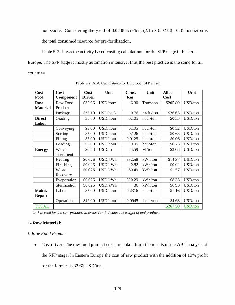
129
hours/acre. Considering the yield of 0.0238 acre/ton, (2.15 x 0.0238) =0.05 hours/ton is
the total consumed resource for pre-fertilization.
Table 5-2 shows the activity based costing calculations for the SFP stage in Eastern
Europe. The SFP stage is mostly automation intensive, thus the best practice is the same for all
countries.
Table 5-2. ABC Calculations for E.Europe (SFP stage)
Cost Pool
Cost Component
Cost Driver
Unit Cons. Res.
Unit Alloc. Cost
Unit
Raw Material
Raw Food Product
$32.66 USD/ton* 6.30 Ton*/ton $205.80 USD/ton
Package $35.10 USD/pack. 0.76 pack./ton $26.63 USD/ton Direct Labor
Grading $5.00 USD/hour 0.105 hour/ton $0.53 USD/ton
Conveying $5.00 USD/hour 0.105 hour/ton $0.52 USD/ton Sorting $5.00 USD/hour 0.126 hour/ton $0.63 USD/ton Filling $5.00 USD/hour 0.0125 hour/ton $0.06 USD/ton Loading $5.00 USD/hour 0.05 hour/ton $0.25 USD/ton Energy Water
Treatment $0.58 USD/m3 3.59 M3/ton $2.08 USD/ton
Heating $0.026 USD/kWh 552.58 kWh/ton $14.37 USD/ton Finishing $0.026 USD/kWh 0.82 kWh/ton $0.02 USD/ton Waste
Recovery $0.026 USD/kWh 60.49 kWh/ton $1.57 USD/ton
Evaporation $0.026 USD/kWh 320.29 kWh/ton $8.33 USD/ton Sterilization $0.026 USD/kWh 36 kWh/ton $0.93 USD/ton Maint. Repair
Labor $5.00 USD/hour 0.2316 hour/ton $1.16 USD/ton
Operation $49.00 USD/hour 0.0945 hour/ton $4.63 USD/ton TOTAL $267.50 USD/ton
ton* is used for the raw product, whereas Ton indicates the weight of end product.
1- Raw Material:
i) Raw Food Product
• Cost driver: The raw food product costs are taken from the results of the ABC analysis of
the RFP stage. In Eastern Europe the cost of raw product with the addition of 10% profit
for the farmer, is 32.66 USD/ton.

130
• Consumed resource: During processing, the raw product loses water, leaving
concentrated solid as the end product. As a result, 15.87% weight of the raw input yields
in the end. Thus (1/0.1587) = 6.3 tons of raw product is needed to get 1 ton of end
product.
ii) Packaging
The end product is sterilized and packed into large containers that can store the food production
while transported to overseas.
• Cost driver: The package cost is 35.10 USD/package.
• Consumed resource: Each package can be filled with 1.32 tons of end product. Thus the
consumed package resource is (1/1.32) = 0.75 packages/ton.
2- Direct Labor:
• Cost driver: The hourly wage for an employee working in a processing plant is estimated
to be 5.00 USD/hour.
• Consumed resource: The amount of time required for each activity is calculated based on
the duration of each operation. The durations are adjusted to the amount of the end
product by considering the amount of product lost through each machine. An example: in
sorting, a worker monitors the raw material as they go through a belt to see if there is any
damaged or unripe product; 50 tons of product can be sorted by a person in an hour. Thus
the consumed time is 0.02 hours/ton of raw product. There is a yield of 15.87% and also
1% of the raw product is lost during sorting. Therefore the consumed time is (0.02 x
0.1587 x 0.99) = 0.126 hours/ton of end product.
131
3- Energy:
i) Electricity
• Cost driver: Electricity costs are calculated by determining the price in each region.
• Consumed resource: The amount of electricity consumed by each machine depends on
the operations. An example: for the evaporation process, 84% of the raw material weight
which consists of water is evaporated to get the concentrated product. The product enters
the process at 74 degrees Celsius temperature. In order for water to evaporate, enough
energy must be used to raise the temperature to 100 Celsius and then convert liquid to
vapor. The specific heat of water is 4.184 kJ/kg.C. Thus (4.184 x 1000 x (100-74)) =
108.78 megaJoules (MJ) of energy is consumed to raise the temperature to 100 Celsius.
To evaporate 84% of it, (334.72 x 1000) = 334.72 MJ of energy is consumed (to make
vapor from one ton of water). The sum is 443.50 MJ which is converted to 123.19 kWh.
Since there is a recovery factor of 50%, a total of (123.19 x 0.50 x 0.84) = 51.66 kWh of
energy is consumed for each ton of raw product entering the evaporation process. The
end product yield is 16%, so the energy needed is adjusted to the end product by dividing
it by 0.16. As a result, 320.29 kWh energy is consumed for each ton of end product
produced.
ii) Water
• Cost driver: Water is listed in the energy category rather than an input, because it is
consumed for washing the product. The price of water used for processing is 0.58
USD/m3.

132
• Consumed resource: 0.57 m3 water are used to wash a ton of entering product; 6.3 tons of
raw product is needed to get one ton of end product. Thus, (0.57 x 6.3) 3.59 m3 water is
consumed for one ton of product.
4- Maintenance and Repair:
i) Labor
• Cost driver: The hourly operator wage rate is 15 USD.
• Consumed resource: Data from an existing plant indicates that labor cost for maintenance
and repair is 75,000 USD/machine for a plant working 85 days per year with a capacity
of 400 ton/hour full shift. The amount of product processed in this plant is calculated to
be (85 x 24 x 400) = 816,000 tons with a yield of (816,000 x 0.1587) = 129,507 tons of
end product. Thus, (75,000 / 15) = 5,000 hours of labor is used to produce 129,509 tons.
(5,000 / 129,507) = 0.0386 hour/ton is needed for maintenance and repair. There are six
machines; therefore total of (0.0386 x 6) = 0.2316 hour/ton is consumed.
ii) Operation
• Cost driver: Operation cost for maintenance and repair is recorded as 100,000
USD/machine for the same plant which operates (85 x 24) = 2,040 machine hours per
year. Thus the cost per machine hour is 49 USD.
• Consumed resource: Since 2,040 hours per machine per year is needed to produce
129,507 tons of end product (2,040 / 129,507) = 0.016 hours is consumed for a ton of end
product. There are six machines, so (0.016 x 6) = 0.0945 machine hours per ton is
consumed. The outcome of the ABC analysis for all of the regions is summarized in
Table 5-3.
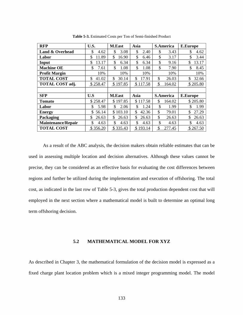
133
Table 5-3. Estimated Costs per Ton of Semi-finished Product
RFP U.S. M.East Asia S.America E.Europe Land & Overhead $ 4.62 $ 3.08 $ 2.40 $ 3.43 $ 4.62 Labor $ 11.89 $ 16.90 $ 6.46 $ 3.17 $ 3.44 Input $ 13.17 $ 6.34 $ 6.34 $ 9.16 $ 13.17 Machine OE $ 7.61 $ 1.08 $ 1.08 $ 7.90 $ 8.45 Profit Margin 10% 10% 10% 10% 10%TOTAL COST $ 41.02 $ 30.14 $ 17.91 $ 26.03 $ 32.66 TOTAL COST adj. $ 258.47 $ 197.85 $ 117.58 $ 164.02 $ 205.80 SFP U.S M.East Asia S.America E.Europe Tomato $ 258.47 $ 197.85 $ 117.58 $ 164.02 $ 205.80 Labor $ 5.98 $ 2.06 $ 1.24 $ 1.99 $ 1.99 Energy $ 56.14 $ 103.10 $ 42.36 $ 79.01 $ 27.29 Packaging $ 26.63 $ 26.63 $ 26.63 $ 26.63 $ 26.63 Maintenance/Repair $ 4.63 $ 4.63 $ 4.63 $ 4.63 $ 4.63 TOTAL COST $ 356.20 $ 335.43 $ 193.14 $ 277.45 $ 267.50
As a result of the ABC analysis, the decision makers obtain reliable estimates that can be
used in assessing multiple location and decision alternatives. Although these values cannot be
precise, they can be considered as an effective basis for evaluating the cost differences between
regions and further be utilized during the implementation and execution of offshoring. The total
cost, as indicated in the last row of Table 5-3, gives the total production dependent cost that will
employed in the next section where a mathematical model is built to determine an optimal long
term offshoring decision.
5.2 MATHEMATICAL MODEL FOR XYZ
As described in Chapter 3, the mathematical formulation of the decision model is expressed as a
fixed charge plant location problem which is a mixed integer programming model. The model

134
combines results from the ABC analysis with other financial and macro-economical data from
public sources.
5.2.1 Model Formulation
In many instances, only the costs of alternatives are included in the objective of an economic
decision model. However, for an offshoring decision, economic conditions of the countries can
have significant impact on cost differences. Therefore, economic indicators such as inflation and
exchange rates should be included by calculating the net present value of cost utilizing
engineering economics principles. The objective value, representing the net present value of the
cost of production/services, is adjusted by incorporating interest inflation, exchange and tax rates
into the total cash flow over the offshoring decision’s life cycle.
Indices:
I= { i = 1,2,….} set of possible supply points
J= { j = 1,2,….} set of demand points
T: Time horizon (annually divided: t = one year) - Tt ∈ represents a one year period
Decision Variables:
Associated with each alternative there are decision variables:
tijx = total amount of production at location i transported to demand location j at period t.
iz = binary variable associated with supply point i, equals 1 if there is production and equals 0 if
there is no production.
135
Assumptions:
• Once the decision is made and the location is selected, the production at that location is not
interrupted for the decision horizon (T).
• The present values of the costs are in USD and remain constant over the decision horizon.
The values change as projected based on the interest, inflation and exchange rates.
• The taxes, duty rates and other trade policy variables remain constant over the decision
horizon.
• Depreciation is calculated linearly along the decision horizon.
• The transfer price (cost of production added with reasonable rate of return) is assumed to be
10% added to the sum of variable and fixed production costs.
• Corporate taxes paid in the destination country is taken into consideration. Tax calculations
in reality should be based on “arm’s length” methodology and the existence of double
taxation treaties between countries. Arm’s length methodology suggests that a corporation
should set the transfer price based on market value. The 10% rate of return is assumed to
obey this convention.
• Each location qhas a maximum supply capacity determined by the climate and economical
conditions of the region.
• The fixed costs (annual fixed expenses and capital) are composed of base portions and
incremental portions expressed as a linear function. The fixed costs linearly increase with the
incremental rate.
• The duties are calculated based on the sum of transfer price and freight costs. In calculating
the duty per item, the fixed expenses are distributed based on the capacity of production.
136
Actual duty rate calculations are more complex involving quotes, subsidies and trade
agreements between countries.
• The expenses are annualized and calculations are based on discrete cash flow analysis.
• The net present value is calculated with a discount based on the interest rates.
Parameters:
M = sufficiently big constant for the binary force constraints (the minimal sufficient constant
should be used to prevent any computational inefficiency)
tjD = the total demand in location j at year t
iv = present variable cost of production/service – taken from the results of the ABC analysis
ijs = present transportation cost from location i to location j (inbound and outbound)
ijd = duty rate for products transported from location i to location j
itx = marginal corporate tax rate in location i
tiq = the cumulative amount of inflation between times 0 and t at location i
tig = forecasted exchange rate between country of location i and USD at time t
te = the cumulative amount of real interest rate between periods 0 and t for USD dollars
0ig = present exchange rate (Foreign Currency / USD) at location i
ifcc = base portion of the annual fixed cost at location i
ik = incremental portion of the annual fixed cost at location i
itcd = base portion of the total capital invested (to be depreciated) at location i
il = incremental portion of the total capital invested at location i
137
iC = capacity limit at location i
Objective Function:
• Variable production cost at location i at time t in local currency:
( ) ∑∈
+=Jj
tijii
ti
ti xvgq 01υ (5-3)
Variable cost at time t at location i in local currency is calculated by first converting the present
cost in USD to local currency and then projecting the result to time t by considering the
cumulative inflation rate.
• Annual fixed cost at location i at time t in local currency:
( ) ⎟⎟⎠
⎞⎜⎜⎝
⎛++= ∑
∈Jj
tijiii
ti
ti xkfccgq 01ϕ (5-4)
Annual fixed cost at time t at location i in local currency is calculated by first converting
the present cost in USD to local currency and then projecting the result to time t by considering
the cumulative inflation rate.
• Total investment capital (to be depreciated) in USD:
∑∑∈ ∈
+=Tt Jj
tijiii xltcdδ (5-5)
The total capital investment consists of the base investment and the incremental capital
increasing with respect to the total production at a location.
138
• Transportation cost from location i to location j at time t in local currency:
( ) tijiji
ti
tij xsgq 01+=ζ (5-6)
• Duty for items from location i to location j at time t in local currency:
( ) tijij
i
iiiiji
ti
tij xs
Cfcc
kvdgq )10.1
10.110.1(1 0 ++++=χ (5-7)
• Corporate tax paid at location i at time t in local currency:
⎥⎦
⎤⎢⎣
⎡+++= ∑
∈Jji
tijiiii
ti
ti fccxkvtxgq 10.0)10.010.0()1( 0τ (5-8)
• Corporate tax deducted at location i at time t in local currency (depreciation value is not
projected over inflation):
⎥⎦
⎤⎢⎣
⎡+= ∑
∈i
Jj
tijii
ti
ti tcdmxltxg )(ω (5-9)
Annual cash flow calculations:
The objective is to minimize the net present value of total costs after taxes. The
parameters are determined either by collecting cost data from the alternative suppliers or by
estimation. These parameters (i.e., variable costs, transportation costs) are expressed in terms of
USD for the initial state of time. Then they are projected to the future by taking into account the
cumulative inflation and exchange rates. The cash flow at a location in local currency can be
represented as shown in Figure 5-3.
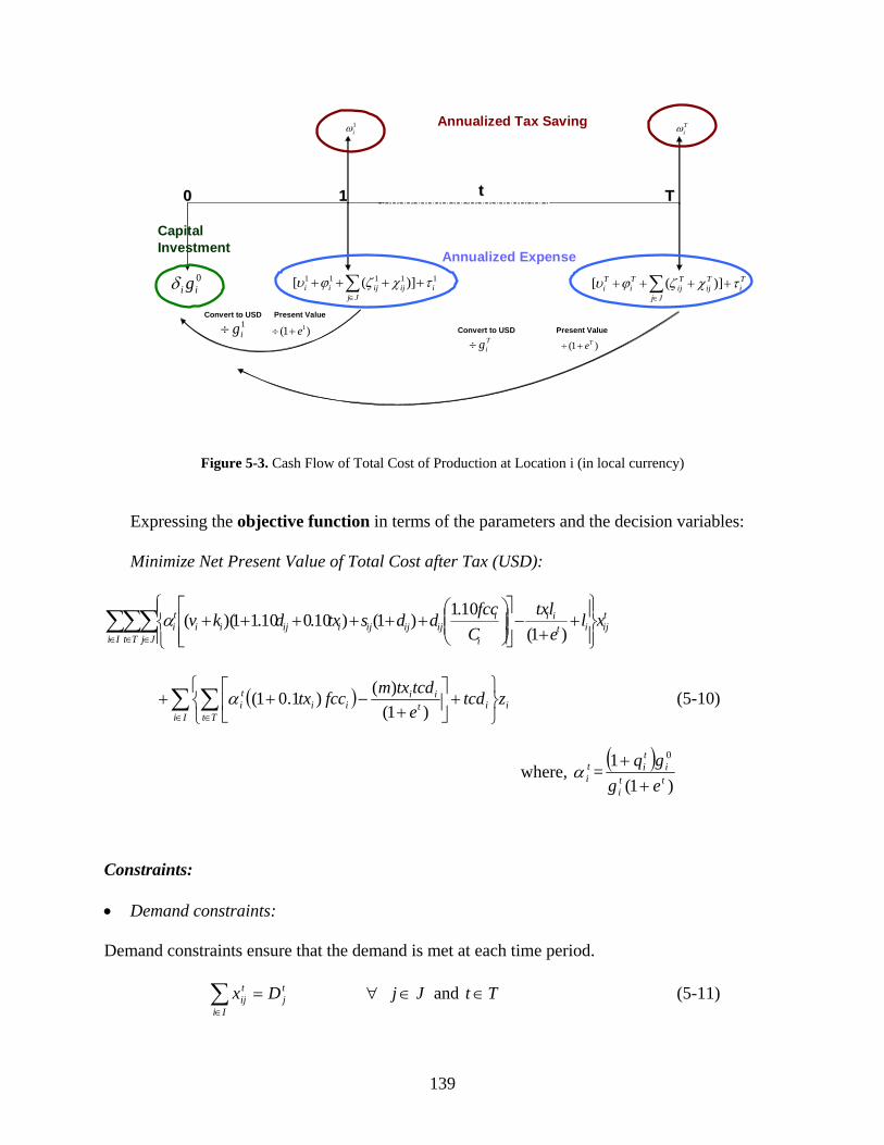
139
0ii gδ 11111 )]([ i
Jjijijii τχζϕυ ++++ ∑
∈
1iω
Ti
Jj
Tij
Tij
Ti
Ti τχζϕυ ++++ ∑
∈
)]([
Tiω
00 11 TTtt
1ig÷ )1( 1e+÷
Convert to USD Present Value
Tig÷ )1( Te+÷
Convert to USD Present Value
Annualized Tax Saving
Annualized Expense
Capital Investment
Figure 5-3. Cash Flow of Total Cost of Production at Location i (in local currency)
Expressing the objective function in terms of the parameters and the decision variables:
Minimize Net Present Value of Total Cost after Tax (USD):
∑∑∑∈ ∈ ∈ ⎪⎭
⎪⎬⎫
⎪⎩
⎪⎨⎧
++
−⎥⎥⎦
⎤
⎢⎢⎣
⎡⎟⎟⎠
⎞⎜⎜⎝
⎛++++++
Ii Tt Jj
tijit
ii
i
iijijijiijii
ti xl
eltx
Cfccddstxdkv
)1(10.1)1()10.010.11)((α
( ) iIi
iTt
tii
iiti ztcd
etcdtxmfcctx∑ ∑
∈ ∈ ⎭⎬⎫
⎩⎨⎧
+⎥⎦
⎤⎢⎣
⎡+
−++)1(
)()1.01(α (5-10)
where, tiα =
( ))1(
1 0
tti
iti
eggq
++
Constraints:
• Demand constraints:
Demand constraints ensure that the demand is met at each time period.
tj
Ii
tij Dx =∑
∈
∀ Jj ∈ and Tt ∈ (5-11)

140
• Capacity constraints:
Capacity constraints ensure that the maximum capacity is not exceeded for each production
location.
iJj
tij Cx ≤∑
∈
∀ Ii ∈ and Tt ∈ (5-12)
• Binary force constraints:
The binary force constraints ensure that production amounts associated for a location is zero if
the location is not chosen.
iTt Jj
tij Mzx ≤∑∑
∈ ∈
∀ Ii ∈ (5-13)
• Trivial constraints:
0≥tijx ∀ Ii ∈ , Jj ∈ and Tt ∈ (5-14)
}1,0{∈tiz ∀ Ii ∈ (5-15)
5.2.2 Data Collection
In XYZ’s case, the five location alternatives for offshoring are denoted by i = 1,2,3,4 and 5,
representing U.S., Middle East, Asia, South America and Eastern Europe respectively. The
demand regions are North America and Western Europe, denoted by j=1 and 2 respectively.
The parameters of the model are set according to the data collected from public and
private sources. The data can be classified into four groups: demand data, cost data, capacity data
and macro-economic indicators. Demand data include the forecasted demand of XYZ sales in the

141
U.S. and Western Europe. The cost data consists of fixed and variable costs of production
associated with each location. Some of the cost values are estimated by the ABC analysis
whereas others are assigned based on data obtained from internal and external sources. The
capacity limits are determined according to the climate and social environment of the regions and
will be described in the next section. The macro-economic indicators include interest rates,
inflation, parities, duty rates and taxes.
A) Demand
The semi-finished product is shipped to the U.S. and Western Europe for further
processing to make the end products; i.e., food condiments sold under a brand name. The total
retail volumes of sauces, dressings and condiments for the decision horizon are presented for
each region in the Table 5-4.
Table 5-4. Forecast Retail Volumes
Total -'000 tons
2004 2005 2006 2007 2008 2009 2010 2011
Western Europe
3,092 3,163 3,222 3,294 3,346 3,410 3,468 3,521
North America
2,723 2,691 2,646 2,583 2,551 2,536 2,535 2,545
Condiments- Avg. 9% of all sauces and condiments Western Europe 278.32 284.67 289.94 296.48 301.15 306.87 312.11 316.89
North America 245.04 242.18 238.15 232.43 229.58 228.20 228.12 229.05
Condiment by XYZ- Avg. 60% share in the U.S. market and 70% in Western Europe Western Europe 194.82 199.27 202.96 207.54 210.80 214.81 218.47 221.82
North America 147.03 145.31 142.89 139.46 137.75 136.92 136.87 137.43
Source: Global Market Information Database by Euromonitor International
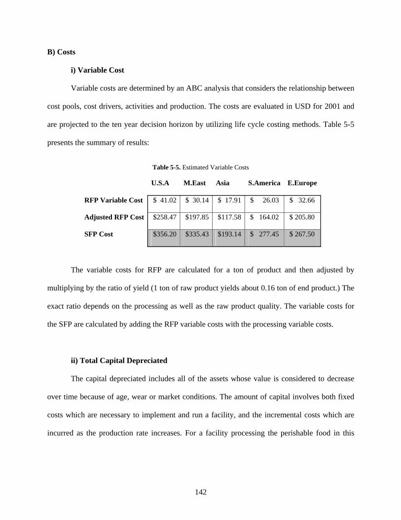
142
B) Costs
i) Variable Cost
Variable costs are determined by an ABC analysis that considers the relationship between
cost pools, cost drivers, activities and production. The costs are evaluated in USD for 2001 and
are projected to the ten year decision horizon by utilizing life cycle costing methods. Table 5-5
presents the summary of results:
Table 5-5. Estimated Variable Costs
U.S.A M.East Asia S.America E.Europe
RFP Variable Cost $ 41.02 $ 30.14 $ 17.91 $ 26.03 $ 32.66
Adjusted RFP Cost $258.47 $197.85 $117.58 $ 164.02 $ 205.80
SFP Cost $356.20 $335.43 $193.14 $ 277.45 $ 267.50
The variable costs for RFP are calculated for a ton of product and then adjusted by
multiplying by the ratio of yield (1 ton of raw product yields about 0.16 ton of end product.) The
exact ratio depends on the processing as well as the raw product quality. The variable costs for
the SFP are calculated by adding the RFP variable costs with the processing variable costs.
ii) Total Capital Depreciated
The capital depreciated includes all of the assets whose value is considered to decrease
over time because of age, wear or market conditions. The amount of capital involves both fixed
costs which are necessary to implement and run a facility, and the incremental costs which are
incurred as the production rate increases. For a facility processing the perishable food in this

143
problem, the total capital depreciation is estimated to have a base cost of 10 million USD. The
incremental cost is estimated by interpolating on the data the obtained from various facilities.
$-$10,000,000$20,000,000$30,000,000$40,000,000$50,000,000$60,000,000$70,000,000$80,000,000$90,000,000
$100,000,000
0 180,000 3,600,000 7,200,000 14,400,000 21,600,000 28,800,000
Total Production (Tons)
Tota
l Cap
ital
Figure 5-4. Capital Costs Interpolated
Therefore, itcd = 10,000,000 USD and il = 3.06 USD/ton for all locations.
iii) Annual Fixed Cost
Annual fixed costs include administrative expenses, indirect labor, insurance and rental.
Although, they are called “fixed,” it is wrong to assume they will remain fixed independent of
the capacity of the facility. Therefore, fixed costs are expressed as having two parts: base cost
and capacity dependent (incremental) costs. Base cost is the total cost that is incurred
independent of the operation of the facility. These include base insurance costs and rental. The
capacity dependent cost is the part that increases incrementally as activity increases.
The annual capital expenses are estimated to equal the amount of annual capital
depreciated linearly. In addition, the insurance cost has a base of 100,000 USD per year plus 1%
of capital. As a result, the annual fixed cost can be expressed as:
000,100)000,000,10(01.1 +÷= Tfcci and 09.3)06.3(01.1 ==ik for all locations.
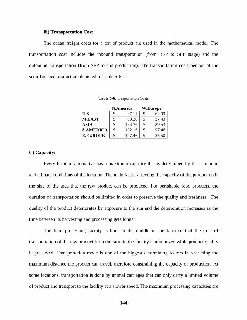
144
iii) Transportation Cost
The ocean freight costs for a ton of product are used in the mathematical model. The
transportation cost includes the inbound transportation (from RFP to SFP stage) and the
outbound transportation (from SFP to end production). The transportation costs per ton of the
semi-finished product are depicted in Table 5-6.
Table 5-6. Trasportation Costs
N.America W.Europe U.S. $ 37.11 $ 62.99 M.EAST $ 99.20 $ 27.43 ASIA $ 164.36 $ 89.53 S.AMERICA $ 102.16 $ 97.46 E.EUROPE $ 107.46 $ 85.50
C) Capacity:
Every location alternative has a maximum capacity that is determined by the economic
and climate conditions of the location. The main factor affecting the capacity of the production is
the size of the area that the raw product can be produced. For perishable food products, the
duration of transportation should be limited in order to preserve the quality and freshness. The
quality of the product deteriorates by exposure to the sun and the deterioration increases as the
time between its harvesting and processing gets longer.
The food processing facility is built in the middle of the farm so that the time of
transportation of the raw product from the farm to the facility is minimized while product quality
is preserved. Transportation mode is one of the biggest determining factors in restricting the
maximum distance the product can travel, therefore constraining the capacity of production. At
some locations, transportation is done by animal carriages that can only carry a limited volume
of product and transport to the facility at a slower speed. The maximum processing capacities are
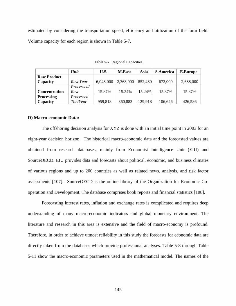
145
estimated by considering the transportation speed, efficiency and utilization of the farm field.
Volume capacity for each region is shown in Table 5-7.
Table 5-7. Regional Capacities
Unit U.S. M.East Asia S.America E.Europe Raw Product Capacity Raw Year 6,048,000 2,368,000 852,480 672,000 2,688,000
Concentration Processed/ Raw 15.87% 15.24% 15.24% 15.87% 15.87%
Processing Capacity
Processed Ton/Year 959,818 360,883 129,918 106,646 426,586
D) Macro-economic Data:
The offshoring decision analysis for XYZ is done with an initial time point in 2003 for an
eight-year decision horizon. The historical macro-economic data and the forecasted values are
obtained from research databases, mainly from Economist Intelligence Unit (EIU) and
SourceOECD. EIU provides data and forecasts about political, economic, and business climates
of various regions and up to 200 countries as well as related news, analysis, and risk factor
assessments [107]. SourceOECD is the online library of the Organization for Economic Co-
operation and Development. The database comprises book reports and financial statistics [108].
Forecasting interest rates, inflation and exchange rates is complicated and requires deep
understanding of many macro-economic indicators and global monetary environment. The
literature and research in this area is extensive and the field of macro-economy is profound.
Therefore, in order to achieve utmost reliability in this study the forecasts for economic data are
directly taken from the databases which provide professional analyses. Table 5-8 through Table
5-11 show the macro-economic parameters used in the mathematical model. The names of the
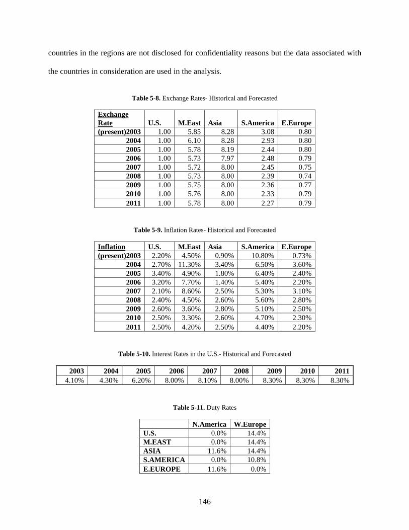
146
countries in the regions are not disclosed for confidentiality reasons but the data associated with
the countries in consideration are used in the analysis.
Table 5-8. Exchange Rates- Historical and Forecasted
Exchange Rate U.S. M.East Asia S.America E.Europe (present)2003 1.00 5.85 8.28 3.08 0.80
2004 1.00 6.10 8.28 2.93 0.80 2005 1.00 5.78 8.19 2.44 0.80 2006 1.00 5.73 7.97 2.48 0.79 2007 1.00 5.72 8.00 2.45 0.75 2008 1.00 5.73 8.00 2.39 0.74 2009 1.00 5.75 8.00 2.36 0.77 2010 1.00 5.76 8.00 2.33 0.79 2011 1.00 5.78 8.00 2.27 0.79
Table 5-9. Inflation Rates- Historical and Forecasted
Inflation U.S. M.East Asia S.America E.Europe (present)2003 2.20% 4.50% 0.90% 10.80% 0.73%
2004 2.70% 11.30% 3.40% 6.50% 3.60% 2005 3.40% 4.90% 1.80% 6.40% 2.40% 2006 3.20% 7.70% 1.40% 5.40% 2.20% 2007 2.10% 8.60% 2.50% 5.30% 3.10% 2008 2.40% 4.50% 2.60% 5.60% 2.80% 2009 2.60% 3.60% 2.80% 5.10% 2.50% 2010 2.50% 3.30% 2.60% 4.70% 2.30% 2011 2.50% 4.20% 2.50% 4.40% 2.20%
Table 5-10. Interest Rates in the U.S.- Historical and Forecasted
2003 2004 2005 2006 2007 2008 2009 2010 20114.10% 4.30% 6.20% 8.00% 8.10% 8.00% 8.30% 8.30% 8.30%
Table 5-11. Duty Rates
N.America W.EuropeU.S. 0.0% 14.4%M.EAST 0.0% 14.4%ASIA 11.6% 14.4%S.AMERICA 0.0% 10.8%E.EUROPE 11.6% 0.0%

147
5.2.3 Solution
The mathematical model when optimized to minimize the total net present value of costs, gives
the optimum objective value of $ 942,712,882 USD total by selecting the U.S., Asia and Eastern
Europe as the regions to implement the production process. The market demand in the U.S. is
fulfilled by the U.S. production facility whereas the Western Europe market is fulfilled by the
production facilities in Eastern Europe and Asia. The results are shown in the Table 5-12.
Table 5-12. Optimal Production Distribution (minimize total net present cost)
to U.S. to W.Europe U.S. plant E.Europe plant Asia plant 2004 147,025 64,903 129,917 2005 145,310 69,350 129,917 2006 142,889 73,038 129,917 2007 139,456 77,620 129,917 2008 137,749 80,885 129,917 2009 136,921 84,891 129,917 2010 136,871 88,556 129,917 2011 137,427 91,907 129,917
Note that the results can easily be interpreted by looking at the cost data that were utilized
in solution of the mathematical model. For Western Europe the production cost in Asia is the
lowest, thus the model first assigns production to the Asia location until the capacity limit is met.
The remaining demand in Western Europe is fulfilled by Eastern Europe facility because the
aggregated production cost with taxes, duties and transportation in Eastern Europe is the next
lowest cost alternative for Western Europe. On the other hand, for the U.S. market, production in
the U.S. comes out to be the most cost advantageous because there are no added duties and
transportation costs are lower.
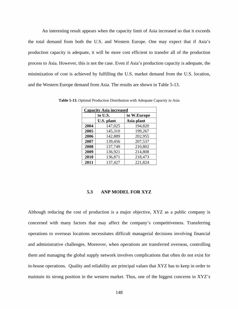
148
An interesting result appears when the capacity limit of Asia increased so that it exceeds
the total demand from both the U.S. and Western Europe. One may expect that if Asia’s
production capacity is adequate, it will be more cost efficient to transfer all of the production
process to Asia. However, this is not the case. Even if Asia’s production capacity is adequate, the
minimization of cost is achieved by fulfilling the U.S. market demand from the U.S. location,
and the Western Europe demand from Asia. The results are shown in Table 5-13.
Table 5-13. Optimal Production Distribution with Adequate Capacity in Asia
Capacity Asia increased to U.S. to W.Europe U.S. plant Asia plant 2004 147,025 194,820 2005 145,310 199,267 2006 142,889 202,955 2007 139,456 207,537 2008 137,749 210,802 2009 136,921 214,808 2010 136,871 218,473 2011 137,427 221,824
5.3 ANP MODEL FOR XYZ
Although reducing the cost of production is a major objective, XYZ as a public company is
concerned with many factors that may affect the company’s competitiveness. Transferring
operations to overseas locations necessitates difficult managerial decisions involving financial
and administrative challenges. Moreover, when operations are transferred overseas, controlling
them and managing the global supply network involves complications that often do not exist for
in-house operations. Quality and reliability are principal values that XYZ has to keep in order to
maintain its strong position in the western market. Thus, one of the biggest concerns in XYZ’s

149
offshoring decision is the possibility of negative reaction from consumers for a food product that
is partly processed outside of the country.
XYZ is also looking for opportunities that can rise as a result of going into a foreign
country. In addition to the organizational and financial benefits, XYZ’s business in developing
countries lead to long term global economic and social effects that in turn may have influence on
XYZ’s market outside of the western world. Although not a significant factor in the decision, it
is worthwhile to include the global consequences as they will affect XYZ’s business in the long
term.
The ANP model is developed to synthesize the intangible factors (including concerns,
benefits and possible opportunities) by evaluating how the decision alternatives contribute to the
factors affecting the outcome of the offshoring process. Each decision alternative (or location in
this case) has a different level of influence in the outcome. For instance a distant production
location from the market creates additional logistical complications when compared to a
production location that is close to the market. Starting a business in a more populated region
may introduce a higher market opportunity compared to starting a business in a less populated
region. As suggested before, in this research the ANP model (like the mathematical model)
captures the decision of whether or not to go offshore by considering “in-house” as an alternative
in the decision model to serve as a baseline of comparison.
As explained in Chapter 3.0 , the intangible factors which XYZ is considering during the
offshoring decision are classified into two: opportunities and risks. Opportunities represent
positive consequences such as benefits arising from emerging markets and prospective
collaborations with outside vendors, whereas risks represent possible negative consequences,
including longer lead times and reduced product quality. The level of opportunity and risk

150
involved in a decision can be described numerically by quantifying all of the contributing
variables. The quantification is achieved by the ANP model where the magnitude of each
alternative’s opportunities and risks are assessed with respect to several criteria. An ANP model
can evaluate the values of opportunities and risks by blending experience, judgment and
historical data using paired comparisons. The next section shows how the ANP is implemented
and used to derive the weights of opportunities and risks for XYZ’s offshoring decision.
First, the criteria that play a role in the decision analysis are determined. The criteria are
further divided into sub-criteria that can separately be considered by the decision maker while
comparing the alternatives. For instance the cluster “risk” can be divided into financial and
operational risks. Financial risks can further be expressed as a combination of market
fluctuations, liabilities and regional economical changes. Such a hierarchy of criteria and sub-
criteria illustrates the spread of influence in the decision making process and allows the decision
maker to identify the extent of influence of the alternatives. The total value of opportunities and
risks associated with each alternative destination are synthesized by considering the alternative
values with respected to the sub-criteria and combining them in the criteria hierarchy with a
bottom to top approach.
5.3.1 Criteria Tree and the Decision Network
For each offshoring decision, the decision criteria should be set individually by considering the
influential factors that will affect the offshoring process. Mainly, all of the factors that create
uncertainty leading to negative consequences are classified under risks whereas all of the factors
that create uncertainty leading to positive consequences are classified under opportunities.
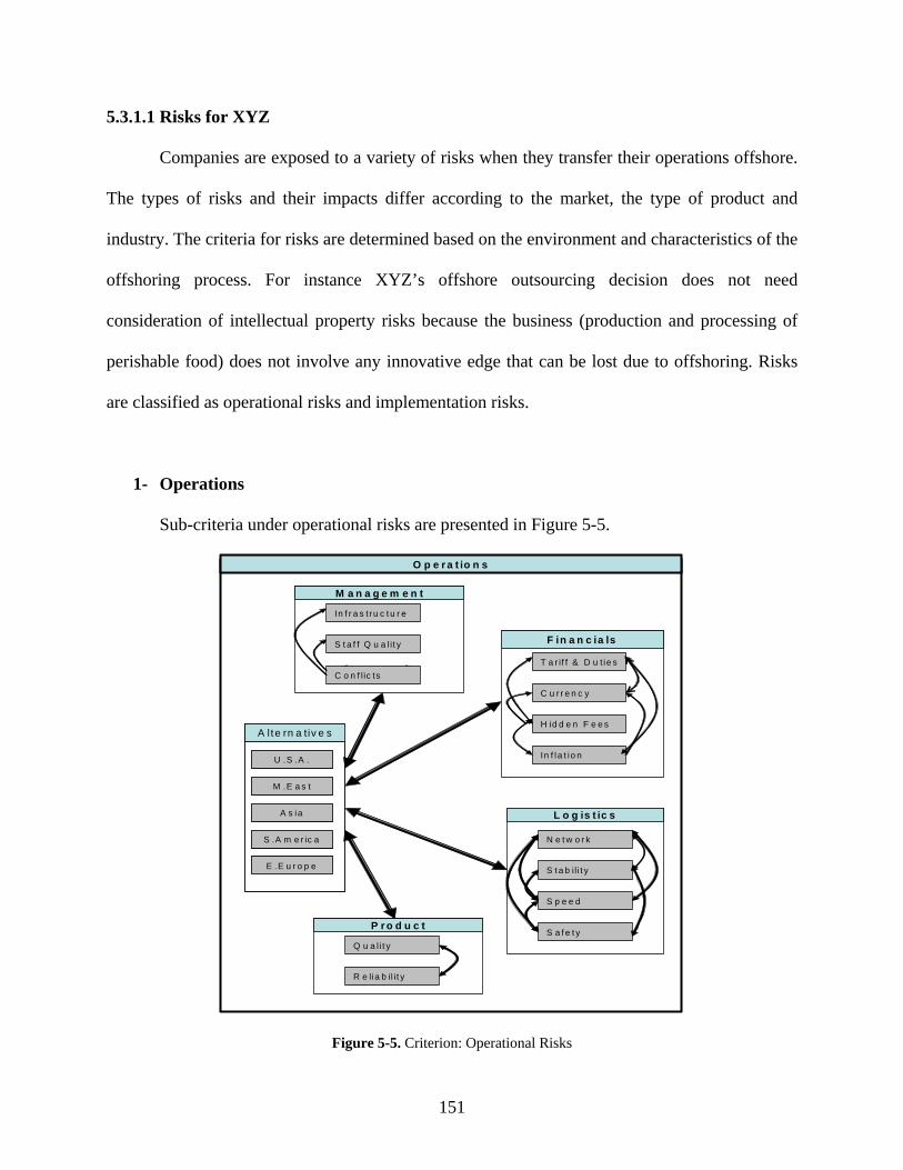
151
5.3.1.1 Risks for XYZ
Companies are exposed to a variety of risks when they transfer their operations offshore.
The types of risks and their impacts differ according to the market, the type of product and
industry. The criteria for risks are determined based on the environment and characteristics of the
offshoring process. For instance XYZ’s offshore outsourcing decision does not need
consideration of intellectual property risks because the business (production and processing of
perishable food) does not involve any innovative edge that can be lost due to offshoring. Risks
are classified as operational risks and implementation risks.
1- Operations
Sub-criteria under operational risks are presented in Figure 5-5.
O p e r a t io n s
T a r if f & D u t ie s
C u r r e n c y
F in a n c ia ls
U .S .A .
M .E a s t
A s ia
S .A m e r ic a
A l te rn a tiv e s
E .E u r o p e
U .S .A .
M .E a s t
A s ia
S .A m e r ic a
A l te rn a tiv e s
E .E u r o p e
H id d e n F e e s
In f la t io n
In f r a s tru c t u r e
S t a f f Q u a l it y
M a n a g e m e n t
C o n f lic ts
N e t w o r k
S t a b ili t y
L o g is t ic s
S p e e d
S a f e t yQ u a li t y
R e lia b il i t y
P r o d u c t
Figure 5-5. Criterion: Operational Risks
152
a) Financial
The financials criterion includes two types of risks: avoidable risks and unavoidable risks.
Unavoidable risks emerge as a result of macroeconomic changes and economic policies of
foreign countries. Some of the macro-economic criteria (such as inflation rates) are
included in the mathematical model as forecasted parameter in calculating the objective
function. However forecasts do not include speculative and drastic changes that may occur
in an economy. The likelihood of such an event happening cannot be known but can be
anticipated based on historical events and the region’s economic and political stability.
Therefore, they are also input into the ANP model.
i. Tariffs and Duties: This is the transaction fee incurred when a commodity is
transported across national borders. The tariff and duty rates are not expected to change
frequently but may be changed by governmental ruling as deemed necessary.
ii. Currency: The currency fluctuations happen as a result of many economic factors that
interact with each other. The exchange rates can be estimated by assuming a steady
economy. However, in some regions extreme events, such as devaluation have occurred
and for these regions such risks should be taken in consideration for future.
iii. Hidden Fees: Hidden fees are costs that were not foreseen in the decision process but
appear during implementation and execution of the decision. Hidden fees in large part
depend on the type of process that is outsourced and the region the operations are located.
Experiences of corporations in certain regions can be used as indicators to estimate the
risk of incurring hidden fees.

153
iv. Inflation: Inflation is an important factor determining the price of raw material, labor
rate and all other expenses. A region with high inflation is an economically unstable
business environment subject to risks.
b) Management
Offshoring may bring managerial risks resulting from inadequate governance, organizational
changes and production deficiencies.
i. Infrastructure: Infrastructural risks arise due to geographical distances and
technological disparities that make communication and control of the processes difficult
to manage.
ii. Staff: With offshoring major organizational changes take place and such changes often
have immense effects on productivity. This can be mitigated by employing change
management principles with technical and communication skills
iii. Conflicts: Conflicts appear as a result of misunderstanding and disagreements within an
organization. As the operations dispense in different locations with different vendors, the
odds for conflicts rise.
c) Product
i. Quality: Quality is the most important factor for consumers especially for a perishable
food product. Even a small decline in the level of quality creates immense risk in the
market.
ii. Reliability: Reliability means the consistency in product quality and on-time delivery.
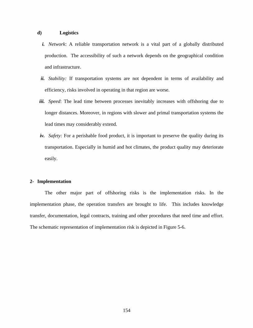
154
d) Logistics
i. Network: A reliable transportation network is a vital part of a globally distributed
production. The accessibility of such a network depends on the geographical condition
and infrastructure.
ii. Stability: If transportation systems are not dependent in terms of availability and
efficiency, risks involved in operating in that region are worse.
iii. Speed: The lead time between processes inevitably increases with offshoring due to
longer distances. Moreover, in regions with slower and primal transportation systems the
lead times may considerably extend.
iv. Safety: For a perishable food product, it is important to preserve the quality during its
transportation. Especially in humid and hot climates, the product quality may deteriorate
easily.
2- Implementation
The other major part of offshoring risks is the implementation risks. In the
implementation phase, the operation transfers are brought to life. This includes knowledge
transfer, documentation, legal contracts, training and other procedures that need time and effort.
The schematic representation of implementation risk is depicted in Figure 5-6.

155
Implementation
Knowledge Transfer
ImplementationU.S.A.
M.East
Asia
S.America
Alternatives
E.Europe
U.S.A.
M.East
Asia
S.America
Alternatives
E.Europe
Training
Management
Investment
Contracts
Figure 5-6. Criterion: Implementation Risks
i. Knowledge Transfer: During the implementation phase, a considerable amount of time
is invested in documentation and communication to transfer the knowledge that exists in-
house. The risks increase as the knowledge transfer gets complicated and massive
because of miscommunication, lack of motivation and capacity.
ii. Training: Training is needed for operators and administrative workers who will be
employed in the offshore location. More training is required when offshoring is done in
regions that lack specialized human and technical capital.
iii. Management: Essential elements for successful implementation are a comprehensive
contract, efficient relationship management, and a structural transition stage. Four basic
management principles are applied: change management, contract management,
stakeholder management, and relationship management. Any deficiency in this stage will
cause failure in the implementation.
iv. Investment: The risk is not the amount of investment that is required; the investment
amount is included while analyzing the cost of the process. Implementation risk consists
of fluctuations in the expenses, the amount of unforeseeable investment that could be
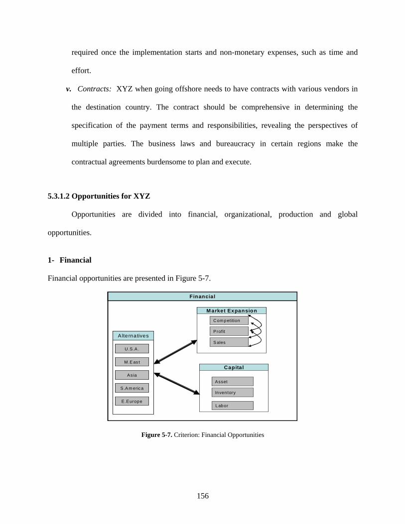
156
required once the implementation starts and non-monetary expenses, such as time and
effort.
v. Contracts: XYZ when going offshore needs to have contracts with various vendors in
the destination country. The contract should be comprehensive in determining the
specification of the payment terms and responsibilities, revealing the perspectives of
multiple parties. The business laws and bureaucracy in certain regions make the
contractual agreements burdensome to plan and execute.
5.3.1.2 Opportunities for XYZ
Opportunities are divided into financial, organizational, production and global
opportunities.
1- Financial
Financial opportunities are presented in Figure 5-7.
Financial
Asset
Inventory
Capital
Com petition
Profit
M arket Expansion
S alesU.S.A .
M.E as t
Asia
S.A m eric a
A lternatives
E.Europe
U.S.A .
M.E as t
Asia
S.A m eric a
A lternatives
E.EuropeLabor
Figure 5-7. Criterion: Financial Opportunities
157
a) Market Expansion
i. Competition: The reduction in production costs are reflected to the market as reduced
prices, adding power to the competitiveness of XYZ brand.
ii. Profit: Cost reductions are not fully reflected to the prices. The difference between the
reduction in cost and prices is gained as an additional profit margin.
iii. Sales: With reduced prices, market share of XYZ can be expected to be higher as the
sales volume and revenue increase.
b) Capital
i. Asset: Machine and capital investments are a part of XYZ’s transfer of production to
overseas. At the same time the in-house assets are considerably reduced with offshoring.
Overall, the asset volume of the company may decline which can be perceived as an
opportunity to elevate return to asset, increasing the shareholder value.
ii. Inventory: The benefit of staying in-house, or transferring operations to a closer
destination is that inventory can be maintained in minimal level with short lead times.
Therefore the probable opportunity value for less distant destinations is higher.
iii. Labor: The cost analysis includes the assessment of low labor rates in alternative
countries. In addition, reduction in labor volume is also a benefit a company may gain in
certain destinations.
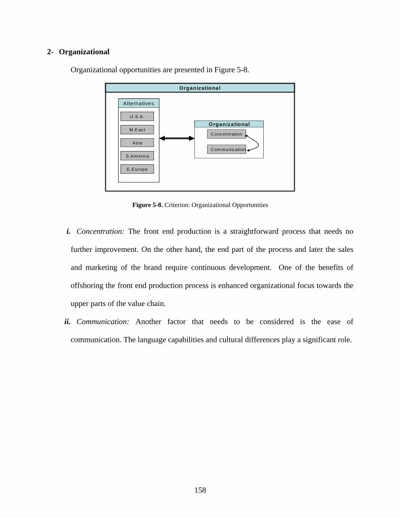
158
2- Organizational
Organizational opportunities are presented in Figure 5-8.
Organizational
Concentration
Com munication
OrganizationalU.S.A .
M.E as t
Asia
S.A m erica
Alternatives
E.Europe
U.S.A .
M.E as t
Asia
S.A m erica
Alternatives
E.Europe
Figure 5-8. Criterion: Organizational Opportunities
i. Concentration: The front end production is a straightforward process that needs no
further improvement. On the other hand, the end part of the process and later the sales
and marketing of the brand require continuous development. One of the benefits of
offshoring the front end production process is enhanced organizational focus towards the
upper parts of the value chain.
ii. Communication: Another factor that needs to be considered is the ease of
communication. The language capabilities and cultural differences play a significant role.

159
3- Production
Production related opportunities include flexibility and productivity as shown in Figure 5-9.
P ro d u c tio n
P rod uc tiv ity
F lex ib ility
P ro d u c tio nU .S .A .
M .E as t
A s ia
S .A m eric a
A lte rn a tive s
E .E urop e
U .S .A .
M .E as t
A s ia
S .A m eric a
A lte rn a tive s
E .E urop e
Figure 5-9. Criterion: Production Opportunities
i. Productivity: Productivity means the efficiency of the production process in terms of
both the amount and the quality of the output. The productivity ranges from region to
region based on the environmental and technical conditions.
ii. Flexibility: Flexibility means being able to make modifications to adjust to the changes
in demand and consumer demands. For instance when the demand spikes at certain times,
flexibility is necessary to increase the production capacity and reduce the transportation
lead time.
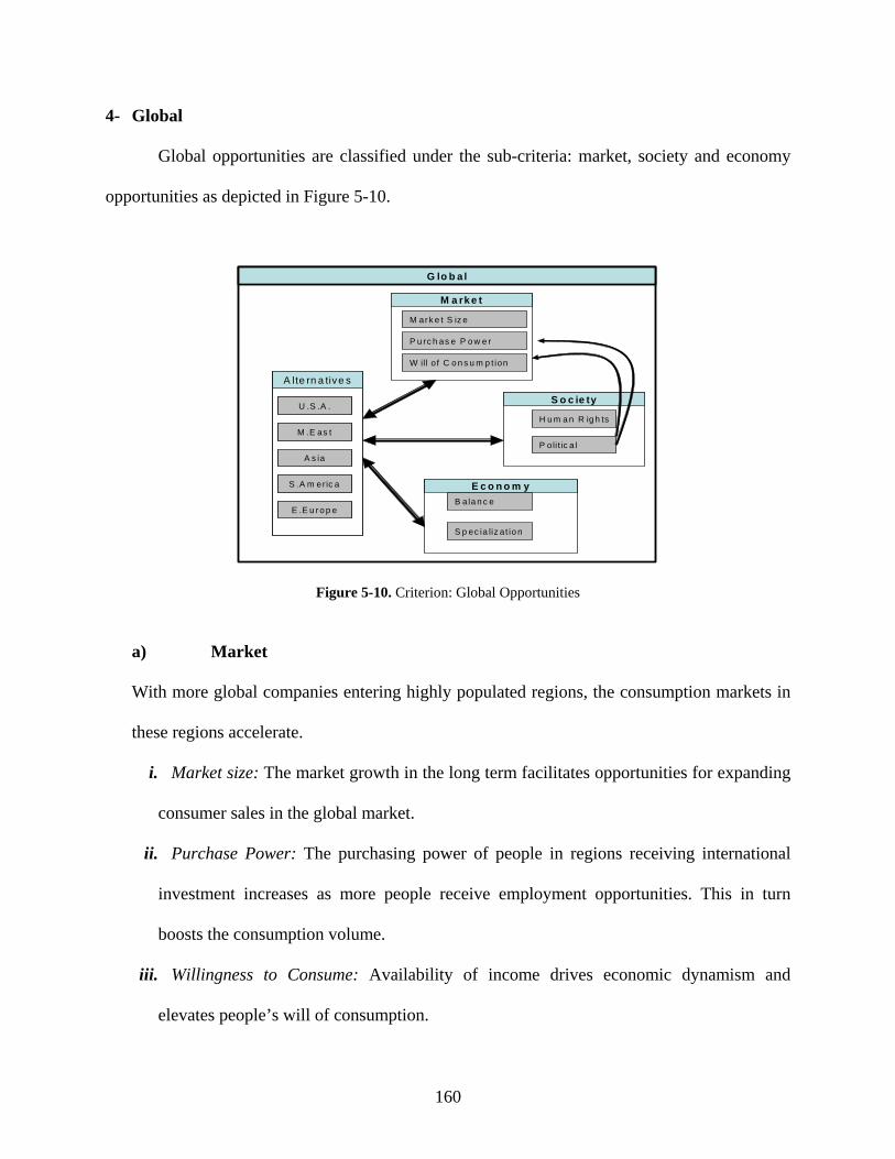
160
4- Global
Global opportunities are classified under the sub-criteria: market, society and economy
opportunities as depicted in Figure 5-10.
G lo b a l
H u m a n R ig h ts
P oli t ic a l
S o c ie tyU .S .A .
M .E as t
A s ia
S .A m eric a
A lte rn a tive s
E .E u ro p e
U .S .A .
M .E as t
A s ia
S .A m eric a
A lte rn a tive s
E .E u ro p eB ala n c e
E c o n o m y
S p ec ia liz at io n
M ark e t S iz e
P u rc h as e P o w e r
M a rk e t
W ill o f C o n s u m p t ion
Figure 5-10. Criterion: Global Opportunities
a) Market
With more global companies entering highly populated regions, the consumption markets in
these regions accelerate.
i. Market size: The market growth in the long term facilitates opportunities for expanding
consumer sales in the global market.
ii. Purchase Power: The purchasing power of people in regions receiving international
investment increases as more people receive employment opportunities. This in turn
boosts the consumption volume.
iii. Willingness to Consume: Availability of income drives economic dynamism and
elevates people’s will of consumption.
161
b) Society
i. Human Rights: The expansion of global trade has social consequences which give rise
to sustainable development of the regions and interdependently help a gradual movement
to protect human rights.
ii. Political: As economies are getting more dependent on each other, an attitude towards
a more democratic and peaceful environment is inevitable.
c) Economy
i. Balance: Industrial advances in developing countries and global trade lead to an
economic balance between regions which in turn ensure a more peaceful environment for
both nations and corporations.
ii. Specialization: In the new global economy countries are beginning to establish
specialized niches leading to growth in productivity, innovation and development.
5.3.2 Data Collection and Paired Comparisons
The paired comparisons are made on a 0-9 scale based on mostly public sources, databases and
literature. Some of the sources are:
• Country macro-economic and social data [109, 110, 111, 112, 113]
The financial and social environment of a country will reflect on the performance of offshoring
processes, consequently defining the success of the business. In the case study presented here, it
is important to note that the agricultural society, its culture and economic status will have direct
effect on the profitability and continuity of production. For instance, in a region where land is
162
owned by individual farmers, it is harder to maintain the product quality and reliability because
common pesticide control cannot be implemented easily. Again, in automation based processes,
the literacy level as well as the technological capabilities determines the ease of implementation.
Databases such as CountryWatch, Europa World and publications by United Nations give
statistical data on the regional economies and social structures. These statistics cannot be directly
applied to paired comparisons in the ANP model but can be synthesized by the decision maker to
make the paired comparisons based on actual data.
Similarly, the economic indicators of a country, such as inflation and trade balance, and
the political conditions demonstrate the stability of the region’s business environment and such
data can be utilized to rate the risks involved in the regions. Opportunities can also be predicted
by looking at the market growth statistics and infrastructural developments. The use of database
statistics in paired comparisons is demonstrated in the following sections.
• Global competitiveness indices [114, 115]
Offshoring is an expanding business practice in many sectors. It attracts attention from
both the corporations seeking a greater competitive edge and consultants that support the
decision processes of corporations as they consider moving their operations offshore. For this
reason, an increasing number of research is conducted to analyze the conditions of doing
business in different countries. Such consulting organizations as McKinsey and AT Kearney and
non-governmental organizations such as World Economic Forum publish competitiveness
indices that rank countries with respect to various aspects (e.g. labor force, education level etc.).
• Agricultural literature [116]
The climate, processing methods, types of diseases and the landscape conditions affect
the productivity and quality of the product. The literature provides a vast pool of resources on

163
measuring agricultural productivity and sustainability in different regions of the world. These
resources serve as valuable tools to compare regions according to their agricultural composition.
• Offshoring publications [117, 118, 119]
Many scholars and professionals carry out extensive research examining and discussing
the drivers, consequences and factors in offshoring. The majority of this research provides
business cases and empirical studies that elucidate the challenges and opportunities of
transferring operations offshore. They also consider the regional difficulties and advantages in
terms of managerial and infrastructural environment and present guidelines to the executives
who are planning to go offshore.
In the ANP decision model, quantification of intangible values is achieved by comparing
the influenced elements with respect to the influence (the criterion). The influence is indicated by
arrows in the network and it determines the structure of paired comparisons that will be made by
the decision maker(s). As discussed above, the paired comparisons, in this empirical study, rely
on public and private data and the opinions of company executives.
Examples of Paired Comparisons:
1- Comparison of alternatives with respect to the “market size” under global opportunities
Although expanding the market outside of the U.S. is not the immediate plan of XYZ, it
will be a future opportunity if the production is transferred to specific regions. Such an
opportunity is not assigned a high weight but it will have minor effects on the decision, therefore
is included in the ANP decision model. The market size opportunity depends on the population
size, competitors in the market and the food culture (the cuisine) of that country. The
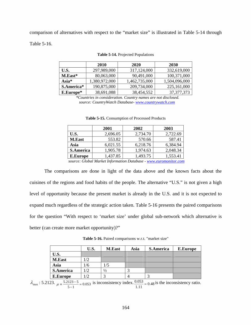
164
comparison of alternatives with respect to the “market size” is illustrated in Table 5-14 through
Table 5-16.
Table 5-14. Projected Populations
2010 2020 2030 U.S. 297,989,000 317,124,000 332,619,000 M.East* 80,063,000 90,491,000 100,371,000 Asia* 1,380,972,000 1,462,735,000 1,504,096,000 S.America* 190,875,000 209,734,000 225,161,000 E.Europe* 38,691,088 38,454,552 37,377,373
*Countries in consideration. Country names are not disclosed. source: CountryWatch Database- www.countrywatch.com
Table 5-15. Consumption of Processed Products
2001 2002 2003 U.S. 2,696.05 2,734.70 2,722.69 M.East 553.82 570.66 587.41 Asia 6,021.55 6,218.76 6,384.94 S.America 1,905.78 1,974.63 2,048.34 E.Europe 1,437.85 1,493.75 1,553.41
source: Global Market Information Database - www.euromonitor.com
The comparisons are done in light of the data above and the known facts about the
cuisines of the regions and food habits of the people. The alternative “U.S.” is not given a high
level of opportunity because the present market is already in the U.S. and it is not expected to
expand much regardless of the strategic action taken. Table 5-16 presents the paired comparisons
for the question “With respect to ‘market size’ under global sub-network which alternative is
better (can create more market opportunity)?”
Table 5-16. Paired comparisons w.r.t. "market size"
U.S. M.East Asia S.America E.Europe U.S. M.East 1/2 Asia 1/6 1/5 S.America 1/2 ½ 3 E.Europe 1/2 3 4 3
maxλ : 5.2123. 053.015
52123.5=
−−
≡μ is inconsistency index. 48.011.1053.0
= is the inconsistency ratio.
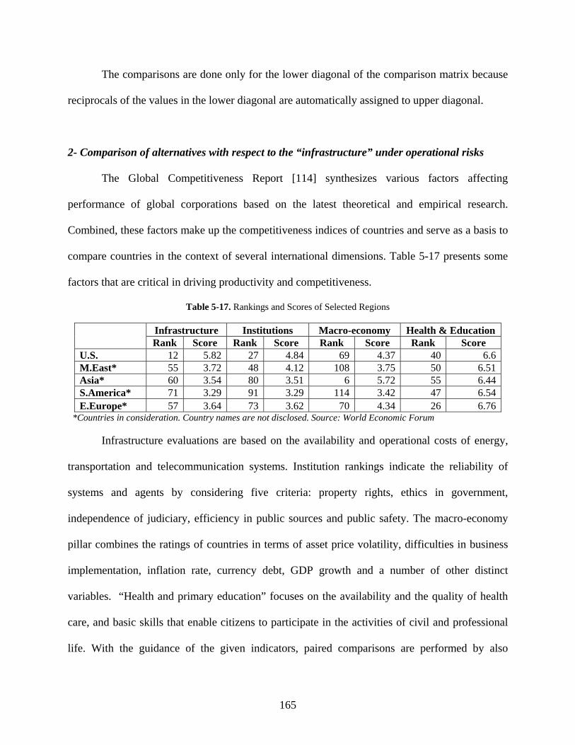
165
The comparisons are done only for the lower diagonal of the comparison matrix because
reciprocals of the values in the lower diagonal are automatically assigned to upper diagonal.
2- Comparison of alternatives with respect to the “infrastructure” under operational risks
The Global Competitiveness Report [114] synthesizes various factors affecting
performance of global corporations based on the latest theoretical and empirical research.
Combined, these factors make up the competitiveness indices of countries and serve as a basis to
compare countries in the context of several international dimensions. Table 5-17 presents some
factors that are critical in driving productivity and competitiveness.
Table 5-17. Rankings and Scores of Selected Regions
Infrastructure Institutions Macro-economy Health & Education Rank Score Rank Score Rank Score Rank Score U.S. 12 5.82 27 4.84 69 4.37 40 6.6M.East* 55 3.72 48 4.12 108 3.75 50 6.51Asia* 60 3.54 80 3.51 6 5.72 55 6.44S.America* 71 3.29 91 3.29 114 3.42 47 6.54E.Europe* 57 3.64 73 3.62 70 4.34 26 6.76
*Countries in consideration. Country names are not disclosed. Source: World Economic Forum
Infrastructure evaluations are based on the availability and operational costs of energy,
transportation and telecommunication systems. Institution rankings indicate the reliability of
systems and agents by considering five criteria: property rights, ethics in government,
independence of judiciary, efficiency in public sources and public safety. The macro-economy
pillar combines the ratings of countries in terms of asset price volatility, difficulties in business
implementation, inflation rate, currency debt, GDP growth and a number of other distinct
variables. “Health and primary education” focuses on the availability and the quality of health
care, and basic skills that enable citizens to participate in the activities of civil and professional
life. With the guidance of the given indicators, paired comparisons are performed by also
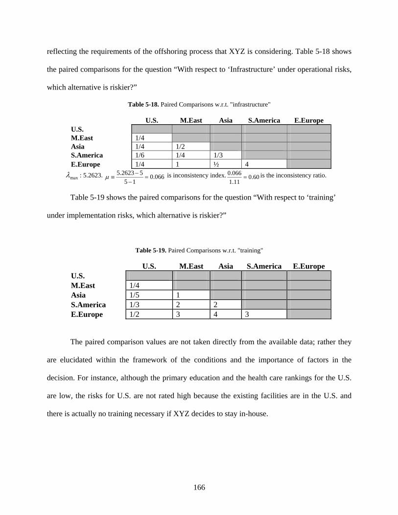
166
reflecting the requirements of the offshoring process that XYZ is considering. Table 5-18 shows
the paired comparisons for the question “With respect to ‘Infrastructure’ under operational risks,
which alternative is riskier?”
Table 5-18. Paired Comparisons w.r.t. "infrastructure"
U.S. M.East Asia S.America E.Europe U.S. M.East 1/4 Asia 1/4 1/2 S.America 1/6 1/4 1/3 E.Europe 1/4 1 ½ 4
maxλ : 5.2623. 066.015
52623.5=
−−
≡μ is inconsistency index. 60.011.1066.0
= is the inconsistency ratio.
Table 5-19 shows the paired comparisons for the question “With respect to ‘training’
under implementation risks, which alternative is riskier?”
Table 5-19. Paired Comparisons w.r.t. "training"
U.S. M.East Asia S.America E.Europe U.S. M.East 1/4 Asia 1/5 1 S.America 1/3 2 2 E.Europe 1/2 3 4 3
The paired comparison values are not taken directly from the available data; rather they
are elucidated within the framework of the conditions and the importance of factors in the
decision. For instance, although the primary education and the health care rankings for the U.S.
are low, the risks for U.S. are not rated high because the existing facilities are in the U.S. and
there is actually no training necessary if XYZ decides to stay in-house.
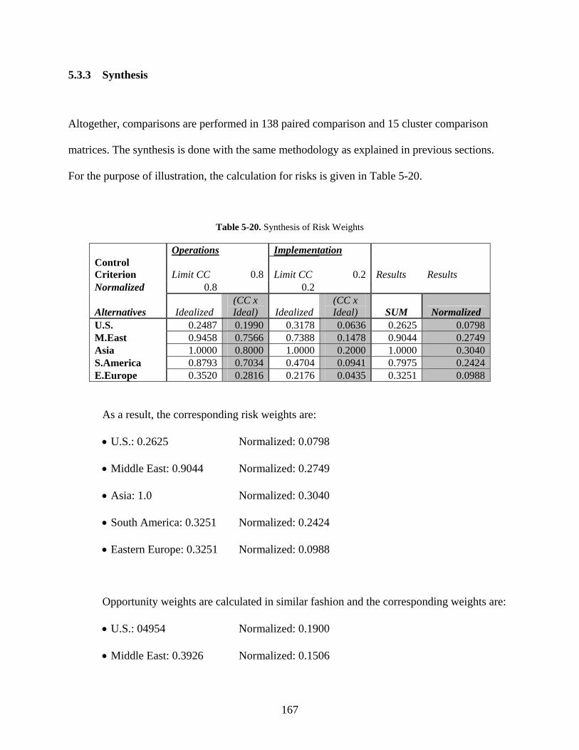
167
5.3.3 Synthesis
Altogether, comparisons are performed in 138 paired comparison and 15 cluster comparison
matrices. The synthesis is done with the same methodology as explained in previous sections.
For the purpose of illustration, the calculation for risks is given in Table 5-20.
Table 5-20. Synthesis of Risk Weights
Operations Implementation Control Criterion Limit CC 0.8 Limit CC 0.2 Results Results Normalized 0.8 0.2
Alternatives Idealized (CC x Ideal) Idealized
(CC x Ideal) SUM Normalized
U.S. 0.2487 0.1990 0.3178 0.0636 0.2625 0.0798M.East 0.9458 0.7566 0.7388 0.1478 0.9044 0.2749Asia 1.0000 0.8000 1.0000 0.2000 1.0000 0.3040S.America 0.8793 0.7034 0.4704 0.0941 0.7975 0.2424E.Europe 0.3520 0.2816 0.2176 0.0435 0.3251 0.0988
As a result, the corresponding risk weights are:
• U.S.: 0.2625 Normalized: 0.0798
• Middle East: 0.9044 Normalized: 0.2749
• Asia: 1.0 Normalized: 0.3040
• South America: 0.3251 Normalized: 0.2424
• Eastern Europe: 0.3251 Normalized: 0.0988
Opportunity weights are calculated in similar fashion and the corresponding weights are:
• U.S.: 04954 Normalized: 0.1900
• Middle East: 0.3926 Normalized: 0.1506
168
• Asia: 0.7175 Normalized: 0.2752
• South America: 0.5471 Normalized: 0.2099
• Eastern Europe: 0.4543 Normalized: 0.1743
5.4 INTEGRAGED MODEL FOR XYZ
There are three objectives in the developed integrated model: minimizing total costs, minimizing
total risks and maximizing total opportunities. Minimization of total costs is achieved by solving
the mathematical model which minimizes the present value of total cost over a decision horizon
subject to demand and capacity constraints. As Section 5.2 indicates, the optimal solution to this
problem is having production plants in Asia, Eastern Europe and the U.S.
The risks in XYZ’s offshoring decision involve mainly macro-economic risks. Even
though there are some implementation risks, their importance weights are much lower.
Therefore, it can be assumed that risks are predominantly diversifiable. On the other hand,
opportunities in large part are based on global and market opportunities, which are
nondiversifiable. Thus, the total risks and opportunities for XYZ in this model are calculated by
taking the average of risk and opportunity values weighted by the production amounts performed
at each location. Thus, the objective of “minimizing total risk” is defined as π2(x) =
∑ ∑∑∑∑∑
∈∈ ∈ ∈
∈ ∈
⎟⎟⎟
⎠
⎞
⎜⎜⎜
⎝
⎛
IiIi Tt Jj
tij
Tt Jj
tij
i x
xRmin and the objective of “maximizing total opportunity” is define as π3(x) =

169
∑ ∑∑∑∑∑
∈∈ ∈ ∈
∈ ∈
⎟⎟⎟
⎠
⎞
⎜⎜⎜
⎝
⎛
IiIi Tt Jj
tij
Tt Jj
tij
i x
xOmax . By replacing the objective function in the mathematical model with
π2(x) and π3(x) one at a time, the optimal solutions for maximum opportunity and risk subject to
demand and capacity constraints are obtained as shown in Table 5-21.
Table 5-21. Optimal Production Distribution (minimize risk and maximize opportunity)
Minimize Risk Maximize Opportunity To U.S. W.Europe U.S. W.Europe
From U.S. U.S. U.S. S.America S.America Asia 2004 147,025 194,820 105,282 41,743 64,903 129,9172005 145,310 199,267 108,014 37,296 69,350 129,9172006 142,889 202,955 109,281 33,608 73,038 129,9172007 139,456 207,537 110,430 29,026 77,620 129,9172008 137,749 210,802 111,988 25,761 80,885 129,9172009 136,921 214,808 155,166 21,755 84,891 129,9172010 136,871 218,473 118,781 18,090 88,556 129,9172011 137,427 221,824 122,688 14,739 91,907 129,917
Therefore, minimization of risks can be achieved by having all of the production at the
less risky location, in the U.S which can satisfy all of the demand required during the decision
horizon. Maximization of opportunities can be achieved by distributing production, starting from
Asia and allocating production to the next opportunistic locations as the capacities permit. The
utopia points (the optimal values for single objective optimizations) give conflicting results as
depicted in Table 5-22.
Table 5-22. Utopio Points
Objective Value Cost Risk Opportunity min.Cost $ 942,712,882 0.1675 0.2181 min. Risk $ 1,114,772,667 0.0798 0.1900 max. Opportunity $ 1,104,697,479 0.2128 0.2278
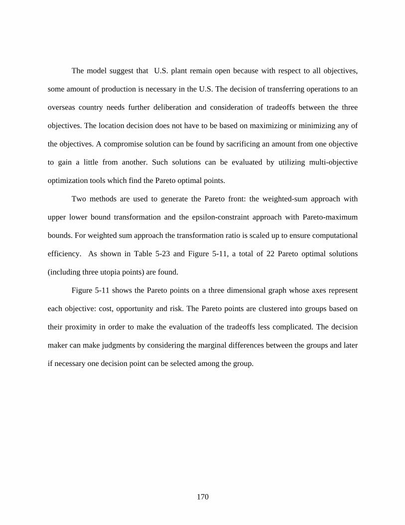
170
The model suggest that U.S. plant remain open because with respect to all objectives,
some amount of production is necessary in the U.S. The decision of transferring operations to an
overseas country needs further deliberation and consideration of tradeoffs between the three
objectives. The location decision does not have to be based on maximizing or minimizing any of
the objectives. A compromise solution can be found by sacrificing an amount from one objective
to gain a little from another. Such solutions can be evaluated by utilizing multi-objective
optimization tools which find the Pareto optimal points.
Two methods are used to generate the Pareto front: the weighted-sum approach with
upper lower bound transformation and the epsilon-constraint approach with Pareto-maximum
bounds. For weighted sum approach the transformation ratio is scaled up to ensure computational
efficiency. As shown in Table 5-23 and Figure 5-11, a total of 22 Pareto optimal solutions
(including three utopia points) are found.
Figure 5-11 shows the Pareto points on a three dimensional graph whose axes represent
each objective: cost, opportunity and risk. The Pareto points are clustered into groups based on
their proximity in order to make the evaluation of the tradeoffs less complicated. The decision
maker can make judgments by considering the marginal differences between the groups and later
if necessary one decision point can be selected among the group.

171
Table 5-23. Pareto Optimal Points- XYZ
Cost Risk Opp. Selected Regions $ 942,712,882 0.1675 0.2181 U.S., Asia, E.Europe $ 943,595,480 0.1628 0.2159 U.S., Asia, E.Europe $ 945,735,349 0.1528 0.2109 U.S., Asia, E.Europe $ 948,125,089 0.1428 0.206 U.S., Asia, E.Europe
Group A
$ 950,884,445 0.1328 0.2011 U.S., Asia, E.Europe Group B $ 951,456,670 0.0912 0.1806 U.S., E.Europe
$ 954,100,581 0.1228 0.1962 U.S., Asia, E.Europe Group C $ 957,602,397 0.1128 0.1913 U.S., Asia, E.Europe Group D $ 970,266,533 0.0897 0.1818 U.S.,E.Europe
$ 973,939,549 0.1652 0.22 U.S., Asia, E.Europe $ 987,777,342 0.1628 0.22 U.S., Asia, E.Europe $ 989,378,032 0.1428 0.21 U.S., Asia, E.Europe Group E
$ 992,469,728 0.1632 0.2217 U.S., Asia, E.Europe $ 993,303,807 0.1228 0.2 U.S., Asia, E.Europe Group F $ 998,978,607 0.1028 0.19 U.S., Asia, E.Europe $ 1,036,179,923 0.1328 0.2102 U.S., Asia Group G $ 1,051,194,558 0.1128 0.2 U.S., Asia, E.Europe
Group H $ 1,055,405,747 0.0928 0.19 U.S., Asia, E.Europe $ 1,077,363,882 0.2028 0.2265 U.S., Asia, S.America $ 1,099,146,067 0.2109 0.2275 U.S., Asia, S.America Group I $ 1,104,697,479 0.2128 0.2278 U.S., Asia, S.America
Group J $ 1,114,772,667 0.0798 0.19 U.S. *Ascending Cost Order
The tradeoffs are assessed by the decision makers to attain a convergence based on their
preferences. Both the relative importance of objectives and the amount of difference in the value
of objectives play a role in making the final decision. First, the decision maker should observe
the maximum and minimum value for each objective. For instance in this problem, the value of
total opportunity changes at most 26% between the least and most opportunistic decision choices
because the opportunity weights associated with alternative locations are similar in value. On the
other hand total risk and total cost vary dramatically with the choice of location.
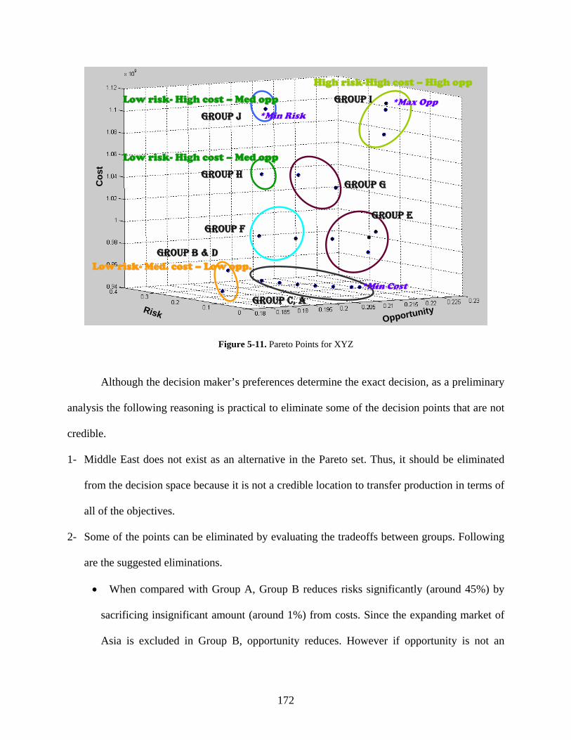
172
OpportunityOpportunityRiskRisk
Cos
tC
ost
Low riskLow risk-- Med. cost Med. cost –– Low Low oppopp..GROUP B & DGROUP B & D
High riskHigh risk--High cost High cost –– High High oppopp
GROUP IGROUP I
GROUP JGROUP J
GROUP HGROUP H
Low riskLow risk-- High cost High cost –– Med Med oppopp
Low riskLow risk-- High cost High cost –– Med Med oppopp
GROUP FGROUP FGROUP EGROUP E
GROUP C, AGROUP C, A
*Min Risk*Max Opp
*Min Cost
GROUP GGROUP G
Figure 5-11. Pareto Points for XYZ
Although the decision maker’s preferences determine the exact decision, as a preliminary
analysis the following reasoning is practical to eliminate some of the decision points that are not
credible.
1- Middle East does not exist as an alternative in the Pareto set. Thus, it should be eliminated
from the decision space because it is not a credible location to transfer production in terms of
all of the objectives.
2- Some of the points can be eliminated by evaluating the tradeoffs between groups. Following
are the suggested eliminations.
• When compared with Group A, Group B reduces risks significantly (around 45%) by
sacrificing insignificant amount (around 1%) from costs. Since the expanding market of
Asia is excluded in Group B, opportunity reduces. However if opportunity is not an

173
important criterion for the corporation, Group A can be eliminated since it escalates the
risks considerably while providing very little cost advantage.
• When compared with Group E, Group I does not provide a significant gain in
opportunity (at most 8%) but it causes both risks and costs to increase significantly.
Unless opportunity is the most important criterion, Group I can be eliminated.
• Adding South America to the selected regions increases opportunity values while
increasing both the risk and cost values. The incremental increase in the opportunity
values by the addition of South America is very small compared to the loss in risks and
costs. Therefore, South America can be eliminated from the decision space.
• If Group E and Group F are compared, one can see that Group E sacrifices significant
amount of risk in return for little gain in opportunity and cost. Therefore, Group E is not
credible.
• Group H, D and B provide similar levels of risks and opportunities while Group H
presents a total cost significantly more than Group D and B. Therefore Group H can be
eliminated.
• Group J (the least risky point) provides the minimum risk by increasing costs
significantly. Group D and Group B sacrifice some from risks to reduce costs and may be
considered instead of Group J. This means, instead of keeping all of the production in the
U.S., XYZ should consider distributing some production to Eastern Europe which may be
more advantageous.
3- Therefore the decision can be reduced to four alternatives: 1- Production only in the U.S.
(high cost, low opportunity, very low risk), 2- Production in the U.S. and Eastern Europe
(medium cost, low opportunity, low risk), 3- Production in the U.S. and Asia (high cost,
174
medium risk and high opportunity) , 4- Production in the U.S., Asia and Eastern Europe
(medium cost, medium risk, high opportunity or high cost, low risk, low opportunity)
4- For the final decision the production schedule should also be reviewed. For instance, the
second point in Group F (cost = $998,978,607, risk = 0.1028, opportunity = 0.19) seems as a
credible alternative. However in this case, production in Asia takes place only for two years.
Therefore, it is not a realistic option.
As a result, the problem is significantly reduced by eliminating the alternatives: Middle
East and South America. Moreover, the analysis clearly suggests that keeping at least a part of
the operations in the U.S. is essential for the optimal decision. The final decision is based on the
company’s objectives and priorities which are determined by exploiting the utilities of costs,
opportunities and risks for XYZ’s stakeholders. In practice, the stakeholders may discuss their
preferences and evaluate the advantages and disadvantages of the alternatives with respect to the
company’s strategic position and vision and find the optimal decision accordingly.
If a more theoretical and scientific approach is needed, utility elicitation methods can be
utilized. The utilities for the alternatives are calculated by adding the utility for the
corresponding objective values and the final decision is made by choosing the alternative which
gives the maximum total utility.
The result is interesting in revealing that two of the alternatives (Middle East and South
America) need not be considered for transferring operations offshore. Moreover, keeping at least
a part of production in the U.S. is essential no matter which objective is prioritized the most.
Without applying the integrated method developed in this study, such a controversial result
would not be expected which would cause a deceptive strategic decision for the company.
175
5.5 INSIGHTS
Figure 5-12 describes the decision process as multiple methods are employed and uncertainty of
the decision reduces while number and type of variables incorporated escalates. The uncertainty
in the beginning involves the uncontrollable uncertainties inherent in the decision problem as
well as the uncertainties due to the intangible variables and cost estimations. The uncontrollable
uncertainties such as the unforeseeable changes in the global economy cannot be eliminated, but
uncertainty can overall be reduced by implementing models that can incorporate intangible
values and provide reliable cost estimation tools.
Math. Model ABC & LCCA ANPMethods
Uncertainty
Quantitative Variables
Time Variables+
+
Quantitative Variables
Quantitative Variables
Qualitative Variables
Time Variables
Integrated Outsourcing Decision Process
Figure 5-12. Decision Process for XYZ
In this case study, when the integrated decision model is applied two of the five
alternatives are eliminated from the decision space because of their inferior objective values. If a
traditional cost analysis is to be performed, one would consider the least costly alternatives,
mainly Asia, Middle East and Eastern Europe. However when all of the facets of the decision are
included by applying the developed integrated method, a contradictory result emerges. Middle

176
East does not appear in any of the non-dominated solutions. All of the non-dominated solutions
include the U.S. alternative even though its production cost (without the addition of
transportation,duties, etc.) is the highest. This means at least a part of the production operations
need to stay in-house.
In conclusion, this empirical study shows the following:
• If offshoring is a long term decision that involves substantial investment, the price quotes
should not be used as a basis of judgment. Instead, the cost of production should be
assessed by utilizing estimation tools (such as ABC) which makes use of economic data
that can reliably be obtained from public databases.
• Although, low production costs in some locations are attractive, adding hidden costs
(such as transportation and duties) reveals that transferring operations to the least costly
regions is not the best strategic decision. Additionally, the decision analysis needs to rely
on life cycle costing of the product in order to incorporate economic indicators in an
international environment.
• In addition to the monetary objectives, the offshoring decision involves many intangible
variables especially for global public companies that operate in multiple locations and
hold considerable shares in multiple markets. The decision should be evaluated from the
perspective of both making the most profit and reducing the risks while opening up
opportunities for future. Employing an integrated method is a necessity for a complex
decision like offshoring.
• With several alternative destinations for offshoring and numerous combinations for
distribution of production, the decision problem gets complicated. An extensive analysis
can help simplify the decision problem by eliminating the inferior alternatives.

177
In summary, this empirical study highlights the necessity for utilizing multiple methods
to incorporate both tangible and intangible variables. It also emphasizes the importance of
applying engineering economic tools in long term offshoring decisions to secure reliability and
accuracy. Most importantly, this empirical study serves as an evidence of the applicability and
usefulness of the developed integrated decision making methodology in offshoring decisions.

178
6.0 SUMMARY AND CONCLUSIONS
Offshoring is a growing trend in today’s global economy. It is a complicated process that leads to
the strategic transformation of a company and affects its organizational structure, the supply
chain system, financial values and many other aspects of the business. Deciding to go offshore
and selecting the best regions and suppliers for operations are challenging tasks that are often
evaluated from financial standpoint without considering other factors which can have far
reaching consequences on the competitiveness of a company.
In this research, an integrated decision approach is developed to incorporate multiple
dimensions of offshoring while taking the life cycle of the decision in consideration. This
integrated decision approach is illustrated through two “real life” cases that have different
characteristics in a similar decision context. In the next section, these two case studies are
compared and the conclusions are drawn from their results. Later, the developed integrated
approach is criticized by evaluating its effectiveness and applicability. The advantages as well as
the disadvantages are presented along with improvement suggestions. In the last sections, related
future research areas are discussed and the contributions of this dissertation to the body of
knowledge are summarized.
179
6.1 COMPARING EMPIRICAL STUDIES
The developed integrated model is applied to two different organizational settings where
offshoring is carried out with different formats considering different product types. The
fundamentals of the decision approach are executed in similar manners. Both problems are
evaluated by incorporating tangible and intangible factors to find the best location (or supplier)
alternatives and the most cost effective distribution of production among these locations. Yet,
there are a number of dissimilarities that require utilization of different methodologies and
modifications in the application of the integrated model. These dissimilarities illustrate how the
developed integrated decision approach can be used in a variety of settings so that a diverse set
of offshoring problems that are commonly faced by today’s corporations can be addressed.
XYZ is a large global public company which is making a location selection for
transformational offshoring involving significant amount of investment over a long time horizon;
whereas SIMA is a mid-size private company that is looking for a specific supplier who can
manufacture products within their innovative design specifications in a very short period of time.
Therefore, in XYZ’s decision model there is an additional monetary uncertainty and complexity
that should be taken into account while analyzing location alternatives. Engineering economic
tools such as Activity Based Costing and Life Cycle Costing are utilized in order to reduce the
cost uncertainties in XYZ’s decision process. On the other hand for SIMA’s decision, offshore
outsourcing is a contractual agreement, so the supplier price quotes can be taken directly as a
basis of calculation.
XYZ’s product is perishable food that requires quality control rather than innovative
design and as a public company, XYZ has to put stakeholder values and global implications into
the criteria set that will determine the risks and opportunities of the regions. Many of these
180
criteria can be assessed by making use of the data and the statistics that are mostly publicly
available. SIMA on the other hand makes fast moving consumer products that require
innovation and need design protection. Thus, the criteria set consists of product and supplier
specific considerations. Therefore, the criteria can be assessed accurately only by company
executives and engineers who acquire extensive knowledge about the product and have
experience with suppliers in overseas.
The approaches followed in the tradeoff analyses differ due to the characteristics of the
problems. In XYZ’s case demand is stable over time and can be forecasted (approximately). The
decision encompasses several years of high volume production that requires initial capital and
investment. Because of its extensive strategic consequences, a change in the total risk value gets
a higher priority than the total cost and the total opportunity. Moreover, within the greater scope
of this decision and also when the size of the company is taken in consideration, slight changes
in the cost are insignificant even though the monetary value of the change may be a very large
amount.
In contrast, SIMA’s total production volume is expected to be lower but it is volatile
depending very much on the product life cycle and the competition in the market. Therefore, it is
desired to have a robust decision whose optimality is maintained with demand changes. During
the product’s life cycle phases, priorities of risks, opportunities and costs change as well. As the
product enters into its mature phase, even slight differences in the cost value become important
because at this stage there is immense price competition. For this reason, small cost differences
play a significant role in decision making. The level of risk averseness is also dependent on the
company’s size and product line and will have affect on how the final decision is made.
181
As a result of the empirical studies, the applicability of the developed integrated decision
approach in diverse settings is illustrated. In both cases, the inferior alternatives are eliminated
from the decision space and the best solutions are identified by incorporating tangible and
intangible values. One of the implications is that although the approach is modified by adding
different methodologies, the basic structure of the decision making process can be employed in a
variety of organizations including private, public, global, local, large and small sized companies.
It can also be applied to long term transformational offshoring as well as short term contractual
offshore outsourcing decisions.
6.2 IMPLEMENTATION AND VALIDATION
The developed integrated decision model provides a tool for decision makers that should be an
improvement over current methods by:
• Presenting multiple “good” solutions whose tradeoffs can be assessed by the decision
maker to attain the best strategic decision.
• Eliminating the bias of intuition by systematically analyzing and incorporating the
intangible variables in a well-established methodology.
• Adding certain important, but often overlooked factors (hidden costs, time variables and
estimations) quantitatively to reduce the inconsistencies that can appear in evaluating
offshore alternatives.
Yet, in order for organizations to implement this integrated model for real world
situations they need to further appraise its strengths and weaknesses. By applying the developed

182
decision approach in two cases, this study demonstrated the model’s applicability and usefulness.
This section will discuss the validation initiatives that were taken during the implementation of
the model on the SIMA and XYZ cases. Later, different approaches will be proposed to escalate
its validation to a higher level.
There is no doubt that validating a model with a significant intangible component is
difficult. Unlike quantitative analysis, qualitative analysis is not a black and white approach.
There are many gray areas that inject subjectivity based on experience and feelings. There is no
“perfect” answer to a decision, such as offshoring, that includes many intangible variables along
with tangible variables which can mostly yield contradictory solutions (e.g.. the least costly
alternative is often the most risky). This research cannot and does not intend to claim that the
solutions resulting from the developed integrated method are the “only” and the “perfect”
solutions. The model itself is an abstraction of the actual setting. Therefore the model needs to be
validated in terms of it being a good abstraction and producing good solutions. Being a good
abstraction means reflecting the decision process accurately whereas good solutions represent
good decisions that direct a corporation to the right offshoring strategy. The validity of the
model also determines the validity of the solution. In summary, in the scope of this research,
validation is defined as “being able to capture the important dimensions of an offshoring decision
in a structured methodology which yields sensible results that can be trusted and respected for
corporations to use in their strategic supply chain and network decisions
In XYZ’s case, the results of the quantitative analysis were utilized by management to
make a decision on where to locate the front-end production process and how much volume to
distribute among these regions. The methodology followed in the analysis was discussed with
the managers and the validity of the methodology and the results were approved. In the end of
183
this analysis the decision makers noted that the final decision would not be based solely on the
quantitative results because qualitative factors needed to be considered. Due to the sensitivity
and confidentiality of the case, the actual decision process implemented by XYZ could not be
pursued further.
For SIMA offshoring decisions involve selecting a supplier who can manufacture the
products in such a manner to meet that product’s short life cycle. Such decisions are strategic but
not long term. Still the consequences of these decisions can be as severe as exiting from the
product market if the supplier fails to provide the required specifications. Such a consequence
has financial implications which can have major effects on this mid-size company. Over the
years, SIMA’s management team developed and refined a management process for selecting and
managing suppliers. Normally (without applying the developed integrated decision approach) the
supplier selection occurs in parallel tracks that are comprised of location, capability and
experience criteria. Ideally a vendor which has a local office is preferred for communication and
documentation convenience but due to the cost considerations, the company often chooses
vendors that quote lower product prices even if they do not have U.S. offices. Then the capability
level of a supplier is assessed by their customer portfolio. Further evaluation is performed on the
selected number of suppliers by assessing their sample products, along with the technical
observations of their manufacturing facilities. Small imperfections in manufacturing capabilities
may be overcome by training and consultancy if the supplier is well-suited and trusted for the
particular product.
During this research, SIMA managers explained that they classify the qualitative
measures under the criterion “experience” since experience is their only indicator that reflects
such measures. Thus, after eliminating the suppliers that do not meet the cost and technical
184
capability standards, SIMA selects the supplier who has been involved in prior business
relationships with SIMA.
Although the experience criterion is a good indicator, SIMA is not always able to find an
experienced supplier for all of the products. Additionally in order to maintain price
competitiveness SIMA may not always be able to choose the most experienced supplier because
there may be other suppliers who offer the same product to SIMA and to the competitors of
SIMA at a much lower price. On the other hand, there is a big risk in working with a new
supplier because of all the unknowns. Thus, supplier selection is a big challenge involving
tradeoffs and uncertainties. Although their existing supplier selection approach gained through
experience has worked well for some products, there is always the chance of missing a good
supplier and losing a competitive edge.
The developed integrated decision approach was attractive to SIMA because they needed
a structured offshore supplier selection process which could present reliable answers by
classifying and evaluating all the factors that are necessary for a successful business relationship.
In this decision model, their existing criteria, such as technical capability and location could be
included in the evaluation of the risks and opportunities associated with the suppliers. Moreover,
the priorities of these criteria, such as insignificance of small imperfections, are incorporated by
assigning weights to them. As a result, the existing intuitive evaluation of suppliers could be
maintained while other factors that normally would be overlooked were captured.
When the managers and employees were introduced to the developed method, they
confirmed that the two-phase approach is a systematic and rigorous approach for analyzing both
the quantitative and qualitative variables. During the implementation of the ANP phase, they
confirmed that most of the results of ANP comply with their intuition while providing a clearer
185
view of the magnitude of the associated intangible factors. There were some counterintuitive
results, too. For instance the risk level of the supplier “Function” was higher than what they had
expected. Normally a U.S. based company would be expected to have lower levels of risks.
However when the criteria under risks were articulated, the results were felt to be realistic.
The results of the case application were confirmed by SIMA. SIMA chose the Taiwanese
supplier (Amberson) for manufacturing of HDMI switchers and in the first phase of the product
life cycle, they encountered success in developing and launching the products in the market.
However, as the market became more competitive, the cost objective gained utmost priority
forcing SIMA to shift production to the lower cost supplier. According to the results, the model
suggests that SIMA negotiate with Amberson to lower the price. SIMA indicated that this
suggestion would be feasible if the demand volumes remain high in the maturity phase. However
the market for HDMI switchers was immediately taken by larger manufacturers and that caused
SIMA’s market share to shrink considerably. In such a price competitive environment,
negotiation with Amberson would not be feasible due to the low projected sale volumes.
The conclusions drawn from the case study were also in line with SIMA’s other
experiences. Interviews with the president indicated that for similar electronic products, the
demand gets higher and it is better to shift production to low cost suppliers as the product goes
into its mature phase. The model revealed that this was not only because of the escalating price
competition but also because with the increasing demand the monetary gains of low cost
suppliers start to even out the higher risks involved with those suppliers. This also became
apparent after several bad experiences which caused major crisis in the company. If such a model
were implemented before, conclusions would be drawn earlier saving the company these
experiences. Another point of validation was the elimination of Hong Kong and the U.S.

186
suppliers. For a majority of product lines, SIMA has been shifting production from Hong Kong
and the U.S to Taiwan and China. The results of the case study justify this shift.
A more extensive validation of the developed integrated decision model can be
performed by applying the methodology in several different settings and later conducting
debriefing sessions where experts can review the model’s competency. The model can further be
enhanced by experimenting on prototypical situations and comparing the approach with other
feasible decision processes that experts use in organizations today. Furthermore, longitudinal
validation lends itself to the offshoring decision to ensure that benefits realized in the short term
are sustained in the long term. Face validation provides a noteworthy reference, but most
important of all the eventual validation of such a developed decision making approach can be
achieved as it is implemented and organizations observe the outcomes of these decisions.
6.3 CRITIQUE
Offshoring is a complicated strategic decision process involving multiple variables, multiple
objectives and multiple stakeholders. The integrated decision approach developed in this
research captures the multi-dimensionality by utilizing different methodologies and blends them
in a decision approach to come up with the best solution alternatives. Yet, one unique solution is
not given to the decision makers as “the” optimal solution. This is the strength of the approach,
rather than a flaw. For such complicated decisions, one cannot expect to obtain a unique solution
that is superior in terms of all of the objectives and variables incorporated in the decision. In fact,
giving one unique solution may be inaccurate and be misleading in a number of ways. Instead,
multiple optimal solutions should be evaluated within a sensitivity analysis framework to

187
structure a decision that is satisfactory from every aspect. In this way, the decision maker can
also see the behavior of the optimal solution with respect to the changes in the parameters and
make his/her decision accordingly.
As illustrated in the empirical studies, one of the several benefits of the integrated
decision approach developed in this study is its ability to eliminate unfavorable offshoring
alternatives from the decision problem. For instance, in XYZ’s case the Middle East is
eliminated from the decision space because Middle East does not appear in none of the “good”
solutions. Again for SIMA, Function and NTC are eliminated from the decision space regardless
of the demand. Elimination of unfavorable alternatives simplifies the decision process by
reducing the number of measures and principles the decision maker needs to consider. It also
provides an opportunity to carry out more accurate decisions by collecting more precise
parameters to input into the model. In XYZ’s case, once the decision problem is reduced further
analysis can be performed by removing some of the assumptions and including other dimensions
(such as the cost of asset reduction in the U.S.) into the problem. In SIMA’s case, once the
decision is reduced to two alternatives, Belton and Amberson, the contractual agreement with the
suppliers may be further negotiated to reach a fair compromise.
A successful start does not always mean that anticipated benefits will continue all the
way through. Loss of direct interactions, distributed supply networks, and cultural differences
challenge achievement of the objective. The complexity of the environment necessitates
continuous monitoring of performance specifications. Any economic, sociologic, or political
alteration in the world can affect the business. Hidden costs behind the operations, such as
logistics and communication costs, are likely to be elevated by a global distortion. Reevaluation
of the offshoring decision should be performed periodically based on industry changes. There is
188
always a possibility that cost-saving expectations may turn into losses due to cost increases or
performance reductions [120]. The developed integrated approach not only provides the tools to
make a strategic offshoring decision but also can be utilized to monitor the performance of that
decision after it is implemented. As actual cost values become apparent and the company gains
experience with the business environment, parameters can be updated to see if the decision
maintains its optimality. If the offshoring process in practice is found to be inferior, the
operations can either be moved to a better location or continued at the same location by
employing improvement initiatives. Since offshoring usually requires long term commitment,
making improvements at the same location may be a more credible option rather than moving the
operations to a different location with the risk of facing new challenges.
The decision approach is primarily developed for application in offshoring decisions to
obtain the optimal location/supplier selections and product/service distributions that will enhance
the competitiveness of a corporation. In addition, this decision approach can be utilized as:
• A tool to give insights on the impacts of different variables in an offshoring decision and
assist management to conceptualize the process before implementing it
• A process for internal management to explain the reasons and implications of offshoring
to the employees by taking account of not only the cost variables but also the intangible
factors
• A basis for negotiations with suppliers and other third party vendors
• A system to control internal and external performance of the offshoring process
• A justification mechanism for upper management
The benefits of the integrated decision approach come with a price. In order to apply this
decision approach, a number of techniques from various disciplines need to be understood.
189
Mathematical programming, multi-objective optimization and Analytic Network Process
modeling are the three essential components of the decision approach. Additional tools such as
ABC and LCC are also employed as needed. Moreover, data collection, model implementation
and solution analysis require time and effort, making the decision process burdensome for
corporations that do not have the resources or the skill sets.
A remedy that may help reduce the method’s complexity is employing simpler
methodologies. For instance replacing Analytic Network Process model with a simpler multi-
criteria decision making method such as Simple Multi-Attribute Rating Technique (SMART) is a
way to simplify the approach. In the SMART technique, a value tree which is similar to ANP’s
criteria network is formed by decomposing the attributes with respect to which the alternatives
are assessed. The attributes need to be independent of each other and free of redundancy.
Alternatives are rated for each attribute beginning from the worst (score of 0) to the best (score
of 100). The attributes are weighted by a technique called “swing weights” and the total value for
each alternative is determined by aggregating the rate of each alternative with the weights of
attributes. The results can be normalized to obtain the normalized weights associated with each
alternative.
A disadvantage of this model is its inability to capture interdependencies among
attributes. The rating method can also be perceived as a disadvantage. Yet, SMART is a much
simpler method that may be preferred in corporate decision making because it requires less
computational time and cognitive effort. For instance in SIMA case, the major complaint was
the large number of paired comparisons required for the ANP model. Moreover, in order to
synthesize the results for ANP, the decision maker has to either calculate the matrix eigenvalues

190
and aggregate them or use the software Superdecisions. In contrast, SMART analysis can easily
be performed on a spreadsheet with straightforward algebraic calculations.
In this research ANP is selected as the multi-attribute decision modeling technique to
quantify intangible values because the paired comparisons method is a realistic approach that can
easily be comprehended by corporate decision makers. Moreover, it can capture
interdependencies and is applicable to complex decisions that include multiple levels of criteria.
On the other hand, different multi-attribute decision modeling techniques may be preferred
depending on the requirements of the decision problem and the decision makers. If the problem
does not involve interdependencies between criteria, simpler multi-attribute decision models can
be utilized. If there is a limited number of criteria and the decision makers are knowledgeable
about probability theory, multi-attribute utility theory may be applied. The choice of the
quantification method also depends on the decision makers’ preferences. In ANP, paired
comparisons are employed as a basis of quantification whereas in other techniques rating, score
assignment and linguistic variables are used to express the values of the intangible variables.
It is important to employ a method for which the decision makers can comfortably
express their ideas. The time and resource restrictions are also important. For instance, in ANP
the paired comparisons take significant time and effort, which may make the method difficult to
apply in cases with time limitations (depending on whether the company is willing to commit the
effort). Some decision models such as utility based methods may not be feasible to apply because
of their theoretical complexity that requires extra knowledge. The accuracy of the decision model
is as well critical and should be investigated.
The integrated decision approach developed in this research provides several benefits to
the corporations that are in the process of deciding whether or not to go offshore, where to
191
transfer operation and in what proportions to distribute production and services among these
locations. The decision model utilizes multiple analytical tools and can be applied to real life
cases as illustrated in the empirical studies. However, its applicability and usefulness may not be
persuasive enough for corporate managers to adapt the approach as a decision support tool
instead of continuing with the traditional cost analysis. Additional effort is needed to introduce
its effectiveness over time.
6.4 FUTURE RESEARCH DIRECTIONS
Uncertainty is inevitable in real life. By the same token, both quantitative and qualitative
variables in offshoring decisions embrace uncertainty. Intuition, expert evaluation, political
factors and other extraneous influences are also intrinsically probabilistic. Thus, uncertainty is
unavoidable for offshoring decisions where the present values are based on an estimate of the
future economic structure and the utilities are determined subjectively. As an extension of this
research, methods may be developed to handle the uncertainty by including elements of
uncertainty and solving the algorithms in a non-deterministic environment.
In a multi-criteria decision problem there are two elements of uncertainty:
1- Inherent uncertainty in both quantitative and qualitative decision variables.
For instance, the present value of an investment depends on economic factors.
2- Subjectivity of the decision maker.
This element is especially important for the qualitative variables where the
quantification is done by the expert evaluation. Experts cannot always be objective
192
while determining the ratio scales of comparison parameters. The probabilistic nature
arising from such subjectivity should be considered in the decision making model.
Inherent uncertainty in quantitative variables can be included in the decision approach in
the mathematical modeling part whereas uncertainty in the qualitative variables can be
represented in the multi-criteria decision modeling part. One way to handle the uncertainty in
quantitative variables is to apply the fuzzy set theory while estimating costs via activity based
costing [121]. Utilizing the fuzzy ABC method enables the decision maker to see the best and
worst case results by calculating cost estimates based on smallest possible, most promising and
largest possible parameters. By solving the decision model with such estimates, the sensitivity of
the decision to different scenarios can be analyzed.
Additionally, the uncertainty in the quantitative variables may be incorporated by
implementing a stochastic mathematical model instead of a deterministic one. In general,
stochastic programs are generalization of deterministic mathematical programs in which some
uncontrollable data are not known with certainty [122]. In stochastic models variables involving
uncertainty are expressed with probability distributions rather than distinct numbers. A stochastic
programming model is formulated in terms of decision stages. First, decisions are taken without
full information, in the latter stages corrective action is taken with full information which is
called recourse. The inherent uncertainty in the qualitative variables can also be handled by
employing probability information into the multi-criteria method.
In offshoring decisions, the decision maker’s attitude directly affects the quantification of
qualitative variables, and therefore determines the numerical values of the intangible criteria
(which are risks and opportunities) associated with the alternatives. One way to handle the
subjectivity of the decision maker is to multiply the decision maker’s judgments (the paired
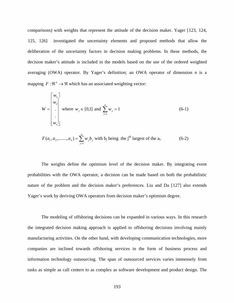
193
comparisons) with weights that represent the attitude of the decision maker. Yager [123, 124,
125, 126] investigated the uncertainty elements and proposed methods that allow the
deliberation of the uncertainty factors in decision making problems. In these methods, the
decision maker’s attitude is included in the models based on the use of the ordered weighted
averaging (OWA) operator. By Yager’s definition; an OWA operator of dimension n is a
mapping ℜ→ℜnF : which has an associated weighting vector:
⎥⎥⎥⎥⎥⎥
⎦
⎤
⎢⎢⎢⎢⎢⎢
⎣
⎡
=
nw
ww
W..2
1
where ]1,0[∈jw and ∑=
=n
jjw
11 (6-1)
∑=
=n
jjjn bwaaaF
121 ),.......,,( with bj being the jth largest of the ai. (6-2)
The weights define the optimism level of the decision maker. By integrating event
probabilities with the OWA operator, a decision can be made based on both the probabilistic
nature of the problem and the decision maker’s preferences. Liu and Da [127] also extends
Yager’s work by deriving OWA operators from decision maker’s optimism degree.
The modeling of offshoring decisions can be expanded in various ways. In this research
the integrated decision making approach is applied to offshoring decisions involving mainly
manufacturing activities. On the other hand, with developing communication technologies, more
companies are inclined towards offshoring services in the form of business process and
information technology outsourcing. The span of outsourced services varies immensely from
tasks as simple as call centers to as complex as software development and product design. The
194
cost structure and the criteria for making offshoring decisions in the service sector differ from
the ones in the manufacturing sector. For instance, service operations may encompass additional
implementation and management cost elements that have significant impact on the total cost.
Furthermore, the cost analysis cannot be performed on product basis, rather it should be based on
activities and processes. The criteria, limitations and priorities also differ and should be
incorporated in the multi-criteria analysis. The offshoring decisions for the service sector can be
evaluated on the foundations of the developed integrated model, however a future research
initiative is necessary to analyze the differences between manufacturing and service offshoring
and adapt the developed integrated model.
Offshore outsourcing is an extensive area that includes many issues that are subject to
further research. Among the plausible operations, determining the right application to offshore
outsourcing is also essential. The products or functions that have already reached maturity are
less risky choices. These applications do not need big changes and can be managed without the
need for direct control. Complexity is also important. More effort is needed to outsource
complex functions. The possibility of failure escalates as the complexity of the job intensifies.
Operations will need close monitoring, which in turn will add to the transaction and
communication costs. Companies may face unsatisfactory negative results if the decision of
which operations to offshoring is not made properly.
Offshoring may also be done in different formats. Linder divides offshore outsourcing
into two categories, conventional and transformational [128]. Conventional outsourcing is
transferring non-core, simple interfaces to another entity whereas transformational outsourcing is
outsourcing to achieve a rapid, sustainable, step-change improvement in enterprise-level
performance. Conventional outsourcing has little flexibility and involves well-understood

195
processes whereas transformational outsourcing involves outsourcing ongoing services that are
critical to the performance of the business. Transformational outsourcing is operationalized by
partnering or investments (do it yourself, merge/acquire or joint venture). In order find the most
appropriate form of offshore outsourcing, a company needs to consider several factors such as
the company’s core competences, industry environment, available options and future goals.
Although these issues (determining the right process and format for offshoring) are
broadly discussed in literature, the number of comprehensive analytical decision models that can
systematical support corporate offshoring decisions is scarce. As globalization accelerates, there
will be more offshoring practices, both successful and unsuccessful, and the necessity of
applying analytical tools for decision making will become more apparent.
6.5 SUMMARY
Traditional methodologies for offshoring decisions are focused on benefit-cost analyses, often
incorporating mathematical programming to determine optimal location selection and
operational distribution. However a strategic decision does not lead to success if made only from
a financial standpoint, excluding potential implications for both the corporation and the
communities.
In this research the traditional decision making approach is expanded by introducing:
• Multi-attribute assessment techniques to incorporate intangible variables that are
important for the welfare of all of the stakeholders.
• Engineering economic tools to realize accurate cost estimations and comprehensive
analysis of the decision over a long time horizon.
196
• Tradeoff analysis to evaluate both tangible and intangible variables for decisions that are
favorable with respect to every aspect of the decision
This research contributes to the literature by developing a novel integrated analytical
decision approach by embracing the strengths of multiple tools to incorporate intangible and
tangible factors with continuous and discrete variables. This decision approach is also
customized to offshoring decisions by exploring the dimensions of offshoring and including the
necessary elements for successful global practices. The application of this integrated decision
approach should not only provide sustainable and better offshoring decisions for the well being
of corporations but also serve as a platform to promote understanding of the key components that
make a prosperous global business structure.
197
BIBLIOGRAPHY
[1] Monczka, R.M., Markham, WJ., Carter, J.R., Blascovich, J.D., & Slaight, T.H. (2005).
Outsourcing Strategically for Sustainable Competitive Advantage. A Joint Study by CAPS Research and A.T. Kearney, Inc.
[2] Friedman, T. L., (2005). The World is Flat: A Brief History of the Twenty-first Century. New York, NY: Farrar, Straus and Giroux
[3] TradeStats Express. Retrieved Feb. 2007 from http://tse.export.gov-
[4] Global Trade Liberalization and the Developing Countries. International Monetary Fund. Retrieved May 2006 from http://www.imf.org/external/np/exr/ib/2001/110801.htm#i November 2001.
[5] Saunders, J. (2003). IT jobs contracted from far and wide. Retrieved Oct. 14, 2003 from www.globeandmail.com.
[6] Schultz, C.L. (2004). Offshoring, Import Competition and the Jobless Recovery. Brookings Institute Policy Brief 136, August 2004.
[7] Bidanda, B., Shuman, L. J., & Arisoy, O. (2005). Manufacturing Outsourcing: Implications for Engineering Jobs & Education. Proceedings of FAIM 2005 Conference. June 2005. Bilboa, Spain.
[8] Farrell, D., Laboissiere M.A., & Rosenfeld, J. (2005). Sizing the Emerging Global Labor Market. The McKinsey Quarterly, No. 3. 93-103.
[9] Young, R., (Producer and Director). (2005). Is Wal-Mart Good for America? PBS Frontline Production
[10] Landis, K.M., Mishra, S., & Porrello K. (2005). Calling a Change in the Outsourcing Market. Deloitte Consulting Publication. April 2005. Retrieved from www.deloitte.com .
[11] Mullin, R. (2006). Managing Outsourced. Journal of Business Strategy. 17(4). 28-38
198
[12] Leggett, K., & Wonacott, P. (2002). The World’s Factory: Surge in Exports from China
Jolts Global Industry. Wall Street Journal. Oct. 10, 2002.
[13] World Bank Data and Statistics. Retrieved October 2006 from www.worldbank.org
[14] Strategic Review 2005. National Association of Software and Service Companies (Nasscom). Retrieved 23 Feb. 2005 from http://www.nasscom.org/strategic2005.asp
[15] Kotabe, M., & Murray, J.Y. (2004). Global sourcing strategy and sustainable competitive advantage. Industrial Marketing Management. 33. 7-14
[16] Deavers, K. (1997). Outsourcing: A Corporate Competitiveness Strategy, Not a Search for Low Wages. Journal of Labor Research. 18(4). 503-519
[17] Bean, L. (2003). The Profits and Perils of International Outsourcing. Journal of Corporate Accounting & Finance. 14(6). 3-10
[18] Weakland, T. (2005). 2005 Global IT Outsourcing Study. DiamondCluster White Paper. Retrieved Spring 2005. www.diamondconsultants.com
[19] Overby, S. (2003). The Hidden Costs of Offshore Outsourcing. CIO Magazine. Sep. 1, 2003
[20] Monczka, R.M., Markham, W.J., Carter, J.R., Blascovich, J.D. & Slaight, T.H. (2005). Outsourcing Strategically for Sustainable Competitive Advantage. A Joint Study by CAPS Research and A.T. Kearney, Inc. accessible from www.atkearney.com
[21] Geoffrion, A.M. (1974). Multicommodity Distribution System Design by Benders Decomposition. Management Science. 20(5). 822-844
[22] Degraeve, Z., & Roodhooft, F.(1999). Effectively selecting suppliers using total cost of ownership. Journal of Supply Chain Management. 35(1). 5-10
[23] Dagraeve, Z., Labro, E., & Roodhooft, F. (2000). An evaluation of vendor selection models from a total cost of ownership perspective. European Journal of Operational Research. 125. 34-58
[24] Muralidharan, C., Anantharaman, N., & Deshmukh, S.G. (2001). Vendor rating in purchasing scenario: a confidence interval approach. International Journal of Operations and Production Management. 21(10). 1306-1325
[25] Amid, A., Ghodsypour, S.H., & O’Brien, C. (2006). Fuzzy multiobjective linear model for supplier selection in a supply chain. International Journal of Production Economics. 104. 394-407
[26] Barbera, S., Hammond, P.J., & Seidl, C. (1998). Handbook of Utility Theory:Volume 2: Extensions. Boston, MA: Kluwer Academic Publishers. 687
199
[27] Min, H. (1994). International Supplier Selection: A Multi-attribute Utility Approach.
International Journal of Physical Distribution & Logistics Management. 24(5). 24-33
[28] SCOR Overview Version 8.0. Supply Chain Council. Retrieved Jan. 2007 from http://www.supply-chain.org
[29] Talluri, S., & Baker, B.C. (2002). A multi-phase mathematical programming approach for effective supply chain design. European Journal of Operational Research. 141. 544-558
[30] Ghodyspour, S.H., & O’Brien, C. (1998). A decision support system for supplier selection using an integrated analytic hierarchy process and linear programming. International Journal of Production Economics. 56-57. 199-212
[31] Weber, C.A., Current, J., & Desai, A. (2000). An optimization approach to determining the number of vendors to employ. Supply Chain Management: An International Journal. 5(2). 90-98
[32] Vidal, C.J., & Goetschalckx, M. (1997). Strategic Production- distribution models: A critical review with emphasis on global supply chain models. European Journal of Operational Research. 98. 1-18
[33] Cohen, M.A. & Mallik, S. (1997). Global Supply Chains: Research and Applications. Production and Operations Management. 6(3)
[34] Arnzten, B.C., Brown, G.G., Harrsion, T.P. & Trafton, L. (1995). Global Supply Chain Management at Digital Equipment Corporation. Interfaces. 25(1). 69-93
[35] Huchzermeier, A., & Cohen, M.A. (1996). Valuing Operational Flexibility Under Exchange Rate Risk. Operations Research. 44(1). 100-113
[36] Nagurney, A., Cruz, J., & Matsypura, D. (2003). Dynamics of Global Supply Chain Supernetworks. Mathematical and Computer Modeling. 37. 963-983
[37] Grossman, G.M., & Helpman, E. (2005). Outsourcing in a Global Economy. Review of Economic Studies. 72(250). 135-159
[38] Kouvelis, P. & Munson, C.L. (2004). Using a Structural Equations Modeling Approach to Design and Monitor Strategic International Facility NetworkS. Pp. 681-798 In Handbook of Quantitative Supply Chain Analysis ed. by Simchi-Levi, D., Wu, D.W., & Shen, Z-J. New York, NY: Springer
[39] Goetschalckx, M., Vidal, C.J., & Dogan, K. (2004). Modeling and design of global logistics systems: A review of integrated strategic and tactical models and design algorithms. European Journal of Operational Research. 143(1). 1-18
200
[40] Steenhuis, H-J., & De Bruijin, E.J. (2004). Assessing Manufacturing Location. Production
Planning and Control. 15(8). 786-795
[41] Bartmess, A., & Cerny, K. (1993). Building Competitive Advantage Through a Global Network of Capabilities. California Management Review. 35(2). 78-102
[42] MacCormack, A.D., Newman, L.J., & Rosenfield, D. (1994). The New Dynamics of Global Manufacturing Site Location. Sloan Management Review. 35(4). 69-80
[43] A.T. Kearney’s 2004 Offshore Location Attractiveness Index (2004). Making Offshore Decisions Retrieved Mar. 2006 from www.atkearney.com
[44] Minevich, M.D., & Richter, F-J. (2005). The Global Outsourcing Report. The CIO Insight Whiteboard. 55
[45] Udo, G.G. (2000). Using analytic hierarchy process to analyze the information technology outsourcing decision. Industrial Management and Data Systems. 100(9). 421-429
[46] Badri, M.A. (1999). Combining the analytic hierarchy process and goal programming for global facility location-allocation problem. International Journal of Production Economics. 62. 237-248
[47] Triantaphyllou, E. (2000). Multi-Criteria Decision Making Methods: A Comparative Study. Boston, MA: Kluwer Academic Publishers
[48] Tamiz, M., Jones, D., & Romero, C. (1998). Goal programming for decision making: An overview of the current state-of-the-art. European Journal of Operational Research. 11(3). 569-581
[49] Saaty, T.L. (1990). How to make a decision: the analytic hierarchy process. European Journal of Oparational Research. 48(1). 9-26
[50] Saaty, T.L. (2004). Fundamentals of the analytic network process- Dependence and feedback in decion-making with a single network. Journal of Systems Science and Systems Engineering. 13(2). 129-157
[51] Yoon, K. (1987). A Reconciliation among Discrete Compromise Solutions. The Journal of Operational Research Society. 38(3). 277-286
[52] Edwards,W., & Barron,F.H. (1994). SMARTS and SMARTER: Improved Simple Methods for Multiattribute Utility Measurement. Organizational Behavior and Human Decision Processes. 60. 306-325
[53] Roy, B. (1991). The outranking approach and the foundations of electre methods. Theory and Decision. 31(1).49-73
201
[54] Sofware information accessible from www.superdecisions.com
[55] Cormen, T.H., Leiserson, C.E., Rivest, R.L., & Stein, C. (2001). Introduction to Algorithms. Second Ed. New York, NY: McGraw- Hill. 981
[56] Dantzig, G.B. (1960). On the Significance of Solving Linear Programming Problems with Some Integer Variables. Econometrica, 28, Jan.1960. 30-44
[57] Nemhauser, G.L., & Wolsey, L.A. (1999). Integer and Combinatorial Optimization. New York, NY: Wiley-Interscience. 236
[58] Balas, E., Ceria, S., & Cornuejols, G. (1996). Mixed 0-1 Programming by Lift-and-Project in a Branch-and-Cut Framework. Management Science. 42(6). 1229-1246
[59] Balas, E., Schmieta, S., & Wallace, C. (2004). Pivot and shift – a mixed integer programming heuristic. Discrete Optimization. 1(1). 3-12
[60] Lokketangen, A., & Glover, F. (1998). Solving 0-1 mixed integer programming problems using tabu search. European Journal of Operational Research. 106. 624-658
[61] Kostikas, K., & Fragakis, C. (2004). Genetic Programming Applied to Mixed Integer Programming. 113-124. In Genetic Programming. Ed. By Keijzer et al. Berlin, Heidelberg: Springer
[62] Belvaux, G., & Wolsey, L.A. (2001) Modeling Practical Lot-Sizing Problems as Mixed-Integer Programs. Management Science. 47(7). 993-1007
[63] Nasr, N., & Elsayed, E.A. (1990). Job shop scheduling with alternative machines. International Journal of Production Research. 28(9). 1595-1609
[64] Beaumont, N. (1997). Scheduling staff using mixed integer programming. European Journal of Operational Research. 98. 473-484
[65] Elson, D.G. (1972). Site Location via Mixed-Integer Programming. Operational Research Quarterly (1970-1977). 23(1). 31-43
[66] Kennington, J.L. (1978). A Survey of Linear Cost Multicommodity Network Flows. Operations Research. 26(2). 209-236
[67] ILOG, Cplex 9.0 Documentation- IloCplex User Manual accessible from www.ilog.com
[68] Saaty, T.L. (2004). Fundamentals of the analytic network process- Dependence and feedback in decision-making with a single network. Journal of Systems Science and Systems Engineering. 13(2). 129-157
202
[69] Saaty, T. L. (2006). Decision Making in Complex Environment. University of Pittsburgh,
lecture notes Spring 2006
[70] Saaty, T. L. (1996). Decision Making with Dependence and Feedback: The Analytic Network Process. Pittsburgh, PA: RWS Publications. 7
[71] Saaty, T. L. (1996). Decision Making with Dependence and Feedback: The Analytic Network Process. Pittsburgh, PA: RWS Publications. 28
[72]Saaty, T. L. (1996). Decision Making with Dependence and Feedback: The Analytic Network Process. Pittsburgh, PA: RWS Publications. 31
[73] Leung, L.C., & Cao, D. (2001). On the efficacy of modeling multi-attribute decision problems using AHP and Sinarchy. European Journal of Operational Research. 132(1). 39-49
[74] Meade, L.M., & Presley, (2002). A. R&D project selection using the analytic network process. IEEE Transactions on Engineering Management. 49(1), 59- 66
[75] Hamalainen, R.P., & Seppalainen, T.O. (1986). The analytic network process in energy policy planning. Socio-Economic Planning Sciences. 20(6). 399-405
[76] Niemira, M.P., & Saaty, T.L. (2004). An Analytic Network Process Model for Financial Crisis Forecasting. International Journal of Forecasting. 20(4). 573-587
[77] Agarwal, A., & Shankar, R. (2003). On-line trust building in e-enabled supply chain. Supply Chain Management. 8(4). 324-334
[78] Braglia, M., Gabbrielli, R. & Miconi, D. (2001). Material Handling Device Selection in Cellular Manufacturing. Journal of Multicriteria Decision Analysis. 10(6). 303-315
[79] Dyer, J.S. (1990). Remarks on the Analytic Hierarchy Process. Management Science. 36 (3). 249-258
[80] Gass, S.I. (2005). Model World: The Great Debate- MAUT versus AHP. Interfaces. An International Journal of Institute for Operations Research and the Management Sciences. 35(4). 308-312
[81] Saaty, T.L. (1990). An Exposition on the AHP in Reply to the Paper “Remarks on Analytic Hierarchy Process”. Management Science. 36 (3). 259-268
[82] Ferrell, K. (2003). Outsourcing’s Benefits May Be More Than Monetary. InformationWeek. Sept. 25, 2003
[83] Minevich, M.D., & Richter, F-J.(2005).Top Spots for Outsourcing.The CIO Insight Whiteboard. March 5, 2005 accessible from www.cioinsight.com
203
[84] http://www.countrywatch.com (Accessible by login)
[85] http://new.sourceoecd.org (Accessible by login )
[86] Sawaragi, Y., Nakayama, H., & Tanino, T. (1985). Theory of Multiobjective Optimization. Orlando, FL: Academic Press
[87] Coello Coello,C.A. (1996). An Empirical Study of Evolutionary Techniques for Multiobjective Optimization in Engineering Design. PhD Thesis. Department of Computer Science. Tulane University
[88] Coello C., Van Veldhuizen D., and Lamont, G., Evolutionary Algorithms for Solving Multi-Objective Problems,Kluwer Academic Publishers, 2002
[89] Coello Coello, C. (2005). Applications of Multiobjective Evolutionary Algorithms. Singapore:World Scientific Publishing Company. 1-23
[90] Marler, T.R. (2005). A Study of Multi-Objective Optimization Methods for Engineering Applications. PhD Thesis, Department of Mechanical Engineering University of Iowa
[91] Ben-Horim, M., & Levy, H. (1980) Total Risk, Diversifiable Risk and Nondiversifiable Risk: A Pedagogic Note. The Journal of Financial and Quantitative Analysis. 15(2).289-297
[92] Ogilvie, J. (2006) Management Accounting and Financial Strategy. CIMA Learning System Strategic Level 2007 series. Burlington, MA: Elsevier.175
[93] Deb, K. (2004). Multi-objective Optimization using Evolutionary Algorithms. New York, NY: John Wiley and Sons. 50-51
[94] Goicoechea, A., Hansen, D.R., & Duckstein, L. (1982) Multiobjective Decision Analysis with Engineering and Business Applications. New York, NY: John Wiley and Sons.
[95] Carmichael, D.G. (1980). Computation of Pareto Optima in Structural Design. International Journal for Numerical Methods in Engineering. 15. 925-952
[96] Cohon, J.L. (1978). Multiobjective Programming and Planning. New York, NY: Academic Press
[97] Koski, J. (1984). Multicriterion Optimization in Structural Design in New Directions. 483-503. In “Optimum Structural Design”, Ed. By Atrek, E., Gallagher, R.H., Ragsdell, K.M.,Zienkiewicz, O.C.
[98] Adapted from a case study performed by Madhavan, R., Bidanda, B., & Arisoy, O. at University of Pittsburgh in 2006

204
[99] Retrieved in April 2007 from www.hdmi.org
[100] Hershey, J.C., & Schoemaker, P.J.H. (1985) Probability versus Certainty Equivalence Methods in Utility Measurement: Are They Equivalent?. Management Science. 31(1). 1213-1231
[101] Bruns, W.J., & Kaplan, R.S. (1987). Accounting & Management: Field Study Perspectives. Boston, MA: Harvard Business School Press, 9., Boston, Mass. 374
[102] Adapted from Needy, K.L. lecture notes “Cost Management”, University of Pittsburgh Spring 2005
[103] Ray, M. R. (1995). Cost management for product development. Journal of Cost Management. 9(1). 52-60
[104] Susman, G. I. (1990)., Product life cycle management: Emerging Practices in Cost Management. Ed. Brinker, B. J. Boston, MA: Warren, Gorham & Lamont. 225-239
[105] OECD Reports on Energy Prices & Taxes. Accessible from www.sourceoecd.org ,
[106] Edwards,W. (2007). Estimating Farm Machinery Costs. Retrieved May 2007 from http://www.extension.iastate.edu/AGDM/crops/html/a3-29.html
[107] Retrieved in Jan. 2007 from www.eiu.com
[108] Retrieved in Jan. 2007 from www.sourceoecd.org
[109] Economist Intelligence Unit (EIU) www.eiu.com (accessible by login)
[110] World Development Indicators www.worldbank.org (accessible by login)
[111] CountryWatch Database www.countrywatch.com (accessible by login)
[112] United Nations Official Document System(ODS) accessible from http://documents.un.org
[113] Europa World Database www.europaworld.com (accessible by login)
[114] Lopez-Claros, A., Altinger, L., Blanke, J., Drzeniek, M., & Mia, I. (2006). The Global Competitiveness Report 2006-2007. World Economic Forum. Sept. 26, 2006.
[115] A.T. Kearney/Foreign Policy Globalization Index. (2006). A.T. Kearney accessed Feb. 2007 from www.atkearney.com
[116] Agricultural Online Access (AGRICOLA) accessible from http://agricola.nal.usda.gov
[117] Power, M., Bonifazi, C., & Desouza, K.C. (2004). The Ten Outsourcing Traps to Avoid. Journal of Business Strategy. 25(2). 37-42
205
[118] Aron, R., & Singh, J.V.(2005) Getting Offshoring Right. Harvard Business Review,
December 2005. 1-10
[119] Hatch, P.J. (2005). Offshore 2005 Research, Preliminary Findings and Conclusions. Ventoro retrieved Mar. 2007 from www.ventoro.com
[120] Bidanda,B., Arisoy, O., & Azim, M. (2007). .14.1 – 14.22. Project Management in Outsourcing Decisions, In “Global Project Management Handbook”. Ed. by Cleland,D.; Gareis, R. New York, NY: McGraw Hill
[121] Nachtmann, H., & Needy, K.L. (2001) Fuzzy Activity Based Costing: A Methodology For Handling Uncertainty in Activity Based Costing. Engineering Economist. 46(4). 245-274
[122] Birge, J.R., & Louveaux, F. (2003). Introduction to Stochastic Programming, New York, NY: Springer Series in Operations Research. 67
[123] Yager, R. R. (1999). Including Decision Attitude in Probabilistic Decision Making. International Journal of Approximate Reasoning. 21 (1). 1-21
[124] Yager, R. R. (2000). Fuzzy Modeling for Intelligent Decision Making Under Uncertainty. IEEE Transactions, Systems Man Cybernet Part B. 30 (1).60-70
[125] Yager, R. R. (2002). On the Valuation of Alternatives for Decision Making under Uncertainty. International Journal of Intelligent Systems. 17. 687-707
[126] Yager, R. R., & Filev, D. P. (1999). Induced Ordered Weighted Averaging Operators. IEEE Transactions, Systems Man Cybernet Part B. 29(2). 141-150
[127] Liu, X., & Da, Q. (2005). A decision tree solution considering the decision maker’s attitude. Fuzzy Sets and Systems. 152. 437-454
[128] Linder, J.C. (2004). Outsourcing for Radical Change: A Bold Approach to Enterprise Transformation. New York, NY: AMACOM. 28