integrated dynamic electric and thermal … · integrated dynamic electric and thermal simulations...

INTEGRATED DYNAMIC ELECTRIC AND THERMAL SIMULATIONS FOR ARESIDENTIAL NEIGHBORHOOD: SENSITIVITY TO TIME RESOLUTION OF

BOUNDARY CONDITIONS

Ruben Baetens1, Roel De Coninck2, 3, Lieve Helsen2 and Dirk Saelens11Building Physics Section, Department of Civil Engineering,

2Applied Mechanics and Energy Conversion Section, Department of Mechanical Engineering,1,2K.U.Leuven, BE-3000 Leuven, Belgium

33E, BE-1000 Brussels, Belgium

ABSTRACTThe sensitivity to time resolution of boundary condi-tions is studied for dynamic integrated simulation ofthermal and electrical networks of a net zero energyresidential neighborhood. Main energy demands orig-inate from domestic electricity consumption of appli-ances and an electricity driven heat pump for spaceheating and domestic hot water production, whereaslocal energy supply is provided by building integratedphotovoltaic (BIPV) systems.Large simultaneity of net power supply at buildinglevel within a residential district results in strong un-derestimation of grid over-voltages for hourly irradi-ance data. The use of minutely meteorological data iscritical for assessment of power losses due to inverterswitch-offs caused by grid voltage increases. On thedemand side, the main deviation is found in a possi-ble correlation of heat pump power demands for SH orDHW but not in the stochastic nature of domestic elec-tricity consumption. Here, sub-hourly demand profilesare less critical if they are not used in grid balancingcontrol strategies at building level.

INTRODUCTIONWith a recent European recast 2010/31/EU oblig-ing to build nearly-zero energy buildings (nZEBs) by2020 (The European Parliament, 2010) and the re-cent communications of the European Commission onthe deployment of a European Smart Grid (EuropeanCommission, 2010), a first step is made towards an in-tegrated approach to tackle climate change while stillmeeting all requests of energy services. Generally,nZEBs face a problem of non-simultaneity betweenlocal energy demand and supply. As such, large scaleimplementation of renewable electricity generation ingeneral and nZEBs in particular will require well de-veloped solutions in the form of energy storage, de-mand side management or both. As such, the planneddevelopments of smart grids and appropriate controlstrategies have to be considered as a necessity for in-tegrated optimization.Simulation-based assessment of the stated problem ofnon-simultaneity requires an integrated multi-domainapproach. Such model is developed in the K.U.Leuven

Energy Institute in Modelica (Baetens and Saelens,2011; De Coninck et al., 2010; Verbruggen et al.,2011) as in fig.1 consisting of the dynamic thermalbuilding response, the dynamics of the domestic hy-dronic heating system, stochastic user behavior andlocal energy supply by means of building integratedphotovoltaic (BIPV) systems in each dwelling, as wellas the low voltage electricity distribution grid betweenthe dwellings. The proposed model differs from exist-ing district models presented in the literature (Heipleand Sailor, 2008; Robinson et al., 2007; Tanimotoet al., 2008; Widen, 2009; Yamaguchi and Shimoda,2010) by combining the dynamics of the hydronic,thermal as well as electric networks at both the build-ing and district level.Within this work, a simulation model dealing withthe grid interaction of residential buildings is set up.The sensitivity of the model is analyzed for varia-tions in time resolution of the applied boundary con-ditions, i.e. residential user behavior and meteoro-logical data influencing the local electricity supply bymeans of BIPVs. Three main reasons may be foundfor the proposed research from a simulation point ofview: First, electricity networks have a much fasterresponse of electricity networks compared to thermalapsects in the built environment which makes electri-cal measures much more sensitive to time resolution ascommon building simulations. Second, the sensitivitygives a first indication of the equivalence of differentassumptions in simulations especially related to dis-tributed generation and energy balancing at buildingdistrict level. Last, the implemented detail strongly in-fluences the amount and detail of required knowledgeon boundary conditions, and the resulting CPU timefor dynamic simulation.In depth comparison allows to formulate an acceptablelevel of required detail and knowledge for the bound-ary conditions of dynamic simulations.

METHODOLOGYAn integrated energy system model for dynamic sim-ulation of a small residential neighborhood of 33dwellings is set up. Herefore, an object-oriented ap-proach based on detailed bottom-up modeling of lo-

Proceedings of Building Simulation 2011: 12th Conference of International Building Performance Simulation Association, Sydney, 14-16 November.

- 1745 -

Figure 1: Representation of the model for integrated dynamic simulation of thermal and electrical energy networksat feeder level. The model includes local electricity generation by means of building integrated photovoltaic(BIPV) systems, stochastic occupant behavior, the thermal building response, the transient behavior of the heating,ventilation and air conditioning system, the building management system (BMS) and the transient response of thelow-voltage electrical distribution grid for a residential neighborhood of 33 dwellings.

cal energy demand and supply has been chosen. Thismodel is simulated using identical parameters but fordifferent time sampling resolution of meteorologicaldata and user behavior. The result is a series of simu-lations of a small district with equal annual electricityand heat demand and production but showing differentresults based on the applied detail in boundary condi-tions. The sensitivity analysis for time resolution ofboundary conditions is carried out towards both elec-trical grid and thermal building performances.Successively, the residential buildings, their thermalnetwork for space heating (SH) as well as domestic hotwater (DHW), and the electrical distribution networkare described.

Residential buildingsFour different detached dwellings as shown in fig.2 areimplemented in the district model. The depicted archi-tectural types of the dwellings are determined as rep-resentative for the Belgian building stock, and are usedin the model based on their statistical spread (Vannesteet al., 2001). With 2010/31/EU (The European Par-liament, 2010) in mind, all dwellings are modeledaccording to a low-energy standard as summarizedin table 1, and as 2-zone (i.e. day and night zone)dwellings for dynamic simulation1. Although only 4different physical building models are implemented,all dwellings will show different results during sim-ulation because of the stochastic user behavior defin-ing the internal gains and the required comfort as ex-plained in Ch..

1Implementation of the dynamic building model is shortly de-scribed in (Baetens and Saelens, 2011). Validation of the modelaccording to ISO 13790 to 13792, and EN 15255 to 15265 is ongo-ing.

Figure 2: Representation of the four architecturaltypes of the implemented dwellings.

All dwellings have an infiltration rate of 0.03 h!1 andmechanically balanced, air-to-air heat-recovery venti-lation (HRV) with an air change rate of 0.5 h!1 anda recovery efficiency of 0.84 (!). To achieve ther-mal comfort in summer conditions, the HRV unit isbypassed when the temperature of the day-zone sur-passes 24"C and is used again when the tempera-ture drops below 19"C. It is supposed that occu-pants open windows when the indoor temperature risesabove 24"C resulting in a natural ventilation rate be-tween 3 and 5 h!1 depending on the available win-dow sizes. Windows are closed again when the in-door temperature drops below 21"C. Summer comfortis further improved by simulating automated exteriorshading by means of a solar screen with a short-wavetransmittance of 0.24 (!) which is lowered at an ir-radiance level of 250 W/m2 and raised again below150 W/m2.

Hydronic heating systemsEach dwelling has a SH and DHW system with iden-tical configuration, consisting of a modulating air-to-water heat pump (HP), a thermal storage tank, a DHWtemperature mixing valve and two radiators, i.e. onefor each building zone as visualized in fig.2. The con-figuration differs for each dwelling on two aspects, i.e.


- 1746 -

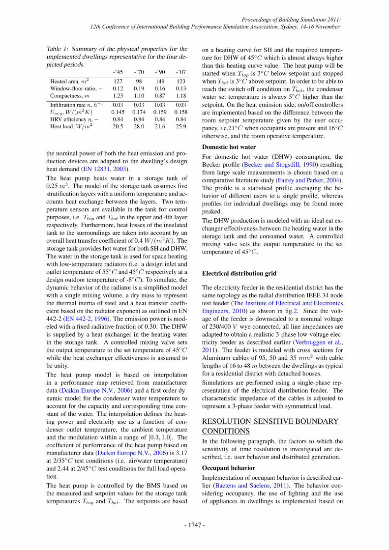
Table 1: Summary of the physical properties for theimplemented dwellings representative for the four de-picted periods.

-’45 -’70 -’90 -’07Heated area, m2 127 98 149 123Window-floor ratio, ! 0.12 0.19 0.16 0.13Compactness, m 1.23 1.10 0.87 1.18Infiltration rate n, h!1 0.03 0.03 0.03 0.03Uavg , W/(m2K) 0.145 0.174 0.159 0.158HRV efficiency !, ! 0.84 0.84 0.84 0.84Heat load, W/m2 20.5 28.0 21.6 25.9

the nominal power of both the heat emission and pro-duction devices are adapted to the dwelling’s designheat demand (EN 12831, 2003).The heat pump heats water in a storage tank of0.25 m3. The model of the storage tank assumes fivestratification layers with a uniform temperature and ac-counts heat exchange between the layers. Two tem-perature sensors are available in the tank for controlpurposes, i.e. Ttop and Tbot in the upper and 4th layerrespectively. Furthermore, heat losses of the insulatedtank to the surroundings are taken into account by anoverall heat transfer coefficient of 0.4 W/(m2K). Thestorage tank provides hot water for both SH and DHW.The water in the storage tank is used for space heatingwith low-temperature radiators (i.e. a design inlet andoutlet temperature of 55"C and 45"C respectively at adesign outdoor temperature of -8"C). To simulate, thedynamic behavior of the radiator is a simplified modelwith a single mixing volume, a dry mass to representthe thermal inertia of steel and a heat transfer coeffi-cient based on the radiator exponent as outlined in EN442-2 (EN 442-2, 1996). The emission power is mod-eled with a fixed radiative fraction of 0.30. The DHWis supplied by a heat exchanger in the heating waterin the storage tank. A controlled mixing valve setsthe output temperature to the set temperature of 45"Cwhile the heat exchanger effectiveness is assumed tobe unity.The heat pump model is based on interpolationin a performance map retrieved from manufacturerdata (Daikin Europe N.V., 2006) and a first order dy-namic model for the condenser water temperature toaccount for the capacity and corresponding time con-stant of the water. The interpolation defines the heat-ing power and electricity use as a function of con-denser outlet temperature, the ambient temperatureand the modulation within a range of [0.3, 1.0]. Thecoefficient of performance of the heat pump based onmanufacturer data (Daikin Europe N.V., 2006) is 3.17at 2/35"C test conditions (i.e. air/water temperature)and 2.44 at 2/45"C test conditions for full load opera-tion.The heat pump is controlled by the BMS based onthe measured and setpoint values for the storage tanktemperatures Ttop and Tbot. The setpoints are based

on a heating curve for SH and the required tempera-ture for DHW of 45"C which is almost always higherthan this heating curve value. The heat pump will bestarted when Ttop is 3"C below setpoint and stoppedwhen Tbot is 3"C above setpoint. In order to be able toreach the switch off condition on Tbot, the condenserwater set temperature is always 5"C higher than thesetpoint. On the heat emission side, on/off controllersare implemented based on the difference between theroom setpoint temperature given by the user occu-pancy, i.e.21"C when occupants are present and 16"Cotherwise, and the room operative temperature.

Domestic hot waterFor domestic hot water (DHW) consumption, theBecker profile (Becker and Stogsdill, 1990) resultingfrom large scale measurements is chosen based on acomparative literature study (Fairey and Parker, 2004).The profile is a statistical profile averaging the be-havior of different users to a single profile, whereasprofiles for individual dwellings may be found morepeaked.The DHW production is modeled with an ideal eat ex-changer effectiveness between the heating water in thestorage tank and the consumed water. A controlledmixing valve sets the output temperature to the settemperature of 45"C.

Electrical distribution grid

The electricity feeder in the residential district has thesame topology as the radial distribution IEEE 34 nodetest feeder (The Institute of Electrical and ElectronicsEngineers, 2010) as shwon in fig.2. Since the volt-age of the feeder is downscaled to a nominal voltageof 230/400 V wye connected, all line impedances areadapted to obtain a realistic 3-phase low-voltage elec-tricity feeder as described earlier (Verbruggen et al.,2011). The feeder is modeled with cross sections forAluminum cables of 95, 50 and 35 mm2 with cablelengths of 16 to 48 m between the dwellings as typicalfor a residential district with detached houses.Simulations are performed using a single-phase rep-resentation of the electrical distribution feeder. Thecharacteristic impedance of the cables is adjusted torepresent a 3-phase feeder with symmetrical load.

RESOLUTION-SENSITIVE BOUNDARYCONDITIONSIn the following paragraph, the factors to which thesensitivity of time resolution is investigated are de-scribed, i.e. user behavior and distributed generation.

Occupant behaviorImplementation of occupant behavior is described ear-lier (Baetens and Saelens, 2011). The behavior con-sidering occupancy, the use of lighting and the useof appliances in dwellings is implemented based on


- 1747 -

Markov-chains and is consistent with the model ofRichardson et al. (Richardson et al., 2010). Bottom-up data concerning household size and installed ap-pliances are determined based on Belgian (FODEconomie, 2008) and European (Richardson et al.,2010) statistics on household sizes and appliance own-ership rates respectively. Based on these data, the out-puts of the model are: presence and activity of thebuilding occupants determining the required thermalcomfort and the use of electric appliances and light-ing resulting in internal heat gains and the real electricpower demand. As such, the occupant behavior influ-ences both the thermal response of buildings and itsgrid impact towards the assessment of distributed gen-eration at feeder level.The original output of the stochastic user profile hasa time resolution of 1 minute. Less detailed boundaryconditions with a resolution of 5, 10, 15, 30 and 60minutes respectively are retrieved as time-arithmeticmeans of the most detailed data.

Distributed generationImplementation of the BIPV system in Modelica is de-scribed earlier (Verbruggen et al., 2011). For localelectricity supply by means of BIPV systems, irradi-ance data with a time resolution of 1 minute are ob-tained artificially using Meteonorm v6.1 for the mod-erate climate of Uccle (Belgium) and the time period1981-2000 based on the Skatveith-Olseth model fordiffuse radiation (Meteotest, 2008). Less detailed so-lar irradiation levels with a resolution of 5, 10, 15,30 and 60 minutes respectively are retrieved as time-arithmetic means of the Meteonorm data in order toobtain equivalent profiles.Sizing of all BIPV systems is based on the total annualelectricity consumption for each dwelling to achieve apredicted level of net ZEB. For this theoretical study,all BIPV systems are modeled to be oriented Southwith an inclination of 34 degrees resulting in the high-est annual production.Due to the resistive character of the feeder, excessivelocal power supply results in an increased feeder volt-age. To avoid excessive voltages, the BIPV system in-verter is curtailed when the voltage at the dwellingsfeeder interface reaches a predefined voltage limit.This limit is set at 110 % of the feeder voltage accord-ing to IEC 60364-6 (IEC 60364-6, 2006). The invertercontrol is given a minimal off-time of 5 min beforetrying to switch on again after voltage disturbances.

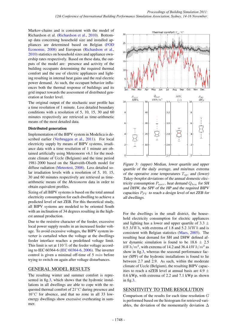
GENERAL MODEL RESULTSThe resulting winter and summer comfort is repre-sented in fig.3, which shows that the hydronic instal-lations in all dwellings are able to cope with the re-quested thermal comfort of 21"C during presence and16"C for absence, and that no zone in all 33 low-energy dwellings show excessive overheating in sum-mer.

Figure 3: (upper) Median, lower quartile and upperquartile of the daily average, and min/max extremaof the operative zone temperatures Top, and (lower)Tukey-boxplot deviations of the annual domestic elec-tricity consumption Puser, heat demand Qhea for SHand DHW, the SPF of the HP and the required BIPVcapacities PPV to reach a design level of net ZEB forall dwellings.

For the dwellings in the small district, the house-hold electricity consumption for electric appliancesand lighting has a lower and upper quartile of 3.3 ±0.5 MWh, with extrema of 1.8 and 5.2 MWh and isconsistent with Belgian statistics (Maes, 2005). Theresulting heat demand for SH and DHW defined af-ter dynamic simulation is found to be 18.6 ± 2.5kWh/m2, with extrema of 14.2 and 36.4 kWh/m2 asshow in fig.3, whereas the seasonal performance fac-tor (SPF) of the hydronic installations is found to liebetween 2.7 and 2.9. As such, within the moderateclimate of Uccle (Belgium), the resulting BIPV capac-ities to reach a nZEB level at annual basis are 4.9 ±0.6 kWp, with extrema of 2.2 and 7.1 kWp as shownin fig.3.

SENSITIVITY TO TIME RESOLUTIONComparison of the results for each time resolution Gis performed based on the histogram for retrieved vari-ables, the deviation of the momentarily deviation !


- 1748 -

Figure 4: (right) Deviations as Tukey-boxplot of themomentarily absolute error ! in time and the Pear-son’s product-moment and Spearman’s rank correla-tion coefficients r, ! for the different implementedtime resolutions G compared to the most-detailed res-olution G1 with 1-minute data, and (left) the overalldensity curve for the resulting power demand and/orinternal heat gain Puser due to occupant behavior (up-per) and the total solar irradiation Psol on a horizontalsurface (lower) respectively.

of the retrieved results, and the Pearson’s product-moment and Spearman’s rank correlation coefficientsr, ! of the retrieved results related to the most detailedassumptions G1 as predicted outcome. Where r de-notes a linear correlation, ! is less sensitive to non-normality of distributions and enables to express theexistence of a correlation between data arrays. Evenfor significant momentarily deviations, possible highcorrelation coefficients may denote that the retrieveddata for most detailed data could be assessed basedon a relationship of retrieved result with less-detaileddata.

Boundary conditionsOccupancy behavior, domestic electricity consump-tion Puser and solar irradiance Psol with different timeresolutions G are used as boundary conditions.Due to the highly stochastic nature of domestic elec-tricity consumption at building level, the impact oftime resolution of user behavior mainly focuses on

peak loads. As shown in fig.4 (upper,left), the over-all occurrence of power loads above 2 kW stronglydiffers. Whereas peak loads up to 8 kW are observedfor a 1-min time resolution G1, the maximum powerloads decrease down to 5 kW for hourly data G60. Al-though the main momentarily error ! (upper,right) isfound small due to the long periods of absence andstandby powers which are unaffected by the time reso-lution, the errors on peak load are also most profoundmomentarily with extrema of 5 kW .Similar analysis can be made for the solar irradiation(see fig.4 (lower)). The deviations on occurrence arefound much smaller and are only found for the 10 %highest irradiations, but the momentarily error raisesup to 0.4 kW/m2 on days with variable weather con-ditions.The depicted error on the extreme loads and the pos-sible large momentarily error may be critical for con-trol algorithms based on the net grid load De Conincket al. (2010). Here, switching on or off the heat pumpis decided based on threshold values of the power bal-ance to improve grid stability by measures at buildingscale. Depending on the sensitivity of time resolution,the use of less detailed data may result in unreliableadjustments and conclusions resulting from control al-gorithms based on dynamic simulations.

Thermal impactAs shown in fig.5 (left), the influence of time reso-lution of boundary conditions on the thermal build-ing response is small. Both annual thermal comfortand electricity consumption of the heat pump for SHand DHW shows little difference for different time fre-quencies.The very high correlation coefficients and the smallmain deviation below 0.2"C of the indoor operativetemperature could be expected from the high thermalinertia of buildings. The small differences are causedby more stable temperature curves and less overshoot-ing by overlapping internal gain peaks and heatinggains for e.g. hourly data. The extrema up to 2.8"Cfor the momentarily deviation of the operative tem-perature are caused by several reasons: (i) shifts intime of the occupancy and thus in switch-on momentsfor SH, (ii) sub-hourly heating patterns which disap-pear in low-frequency boundary conditions and (iii)triggering (or not) of temperature-based control sig-nals e.g. for opening of windows. The latter may beenforced by not taking into account the time constantof controllers in the simulations, whereas the first tworeasons result from coupling the heating pattern to thestochastic occupancy profile.Similar reasons cause large momentarily differences! in the heat pump power up to 3 kW . The largedrop of the Pearson’s product moment correlation co-efficient r down to 0.2 might suggest that the heat-ing sequences of the residential building completelydiffer for the different time resolutions, whereas the


- 1749 -

Figure 5: (right) Deviations as Tukey-boxplot of themomentarily absolute error ! in time and the Pear-son’s product-moment and Spearman’s rank correla-tion coefficients r, ! for the different implementedtime resolutions G compared to the most-detailed res-olution G1 with 1-minute data, and (left) the over-all density curve for the resulting indoor operativetemperatures Top (upper) and the resulting heat pumppower PHP (lower) for SH and DHW respectively.

higher Spearman’s rank correlation coefficient mightsuggest differently. Closer investigation of the heatpump power shows that the large extrema for momen-tarily deviations are caused by (i) time shifts in theheat pump control signals due to deviations in the oc-cupancy profile and (ii) a variance in cycling of theheat pump when comfort is met as not all heating-upperiods are equally long. The different switch-on and-off moments result in the rather high spread on themomentarily deviation as the heat pump power PHP

changes during the heating cycle in each dwelling,whereas the very low correlation factors are caused bythe large discontinuity of heat pump power pattern.The depicted effects might not solely be assigned totime resolution as it is not the information source ofa control algorithm but mainly its result. Within thesimulations, required thermal comfort and SH controlis coupled to the stochastic occupancy profile, whereasreal-life heating patterns are defined by a combina-tion of stochastic behavior and fixed daily householdhabits. Furthermore, current heating systems control

may no longer apply for nZEBs due to reduced (sys-tem and) control efficiencies of hydronic systems forlow heat demands .

Electrical impactThe sensitivity of the electrical impact towards timeresolution is found to be more profound in contrast tothe effect on thermal aspects. The reason is found inthe very fast response time of electrical systems com-pared to thermal effects, but also in the responsive-ness which is defined by both the sensitivity of domes-tic electricity consumption and local electricity gen-eration, as well as the effect of the heat demand forSH and DHW by means of the electricity driven heatpump.

Feeder loads and voltagesAs shown in fig.6 (upper, left), the main deviation onannual base of the net power exchange of a dwelling ismainly made on the net power demand side (denotedby negative values). The overall occurrence of powerloads of 2 to 8 kW strongly deviates and differs fromthe sensitivity of the boundary conditions as shown infig.4 as it includes the electric power demand of theheat pump which coincides with local domestic de-mand. Although the main momentarily deviation !(upper, right) is small due to the long periods of ab-sence unaffected by time resolution, the deviations onpeak load are also found here most profound momen-tarily with extrema up to 9 kW . The high maximumdeviation is due to the correlation between domesticelectricity demands and heat demands at arrival.A smaller deviation is noticed in the occurrence of ahigher net supply (denoted by positive values in fig.6(upper, left)) for 1-minute data compared to hourlydata, whereas the maximum supply is found equal forall data.More importantly, the resulting conclusion on thephysical impact of this net power exchange can befound opposite as depicted for this net power exchangein fig.6 (lower). As shown in fig.6 (lower, left), thelargest deviation is made on the over-voltage of thegrid due to excessive BIPV generation and a result-ing net supply. Here, hourly data G60 result in anunderestimation up to 9V on a maximum daily over-voltages of 18 V compared to the feeder voltage forG1, i.e. a relative deviation of factor 2. The strongunderestimation resulting from the small deviation onthe net power supply at building level is due to thestrong correlation in time of net power supply at feederlevel and a resulting strong accumulation of voltageincreases. Contradictory to the large underestimationof peak power demands at building scale comparedto 1-minute stochastic data G1 (fig.6 (upper, left)),no lower extreme under-voltages are found for hourlysimulations due to the stochastic nature and resultingweak coincidence in time of net power demand. Assuch, the depicted deviation on building scale will notresult in underestimation of grid voltage drops.


- 1750 -

Figure 6: (right) Deviations as Tukey-boxplot of themomentarily absolute error ! in time and the Pear-son’s product-moment and Spearman’s rank correla-tion coefficients r, ! for the different implementedtime resolutions G compared to the most-detailed res-olution G1 with 1-minute data, and (left) the overalldensity curvefor the net electrical power balance atbuilding level Pnet (upper) and the distribution gridvoltage VAC (lower) respectively. Negative values forPnet depict a net demand, positive values a net supplyto the feeder.

Generation lossesWithin this case, the deviation caused by time reso-lution on the increased feeder voltages strongly influ-ences the BIPV generation losses caused by BIPV cur-tailment (and vice versa) at the threshold voltage of253 V as shown in fig.7. The total annual generationloss at feeder level is found 3.6 MWh for G1 wherethis value drops for larger time resolutions to 1.9 MWhfor G60 denoting a strong underestimation of 46% atfeeder level. The total loss denotes 2.5% of the annualdemand for G1 and 1.4% for G60.With a one-minute time resolution G1, 15 of the 33dwellings in the neighborhood suffer from generationlosses (depending on their location within the feedertopology) by BIPV curtailment, compared to 12 forG60. The low number of dwellings indicate that thedepicted error on the level of an individual dwellingwill be larger than on feeder level. When only thedwellings which suffer from curtailment are assumed,the generation losses at level of an individual dwelling

Figure 7: The overall density curve for the result-ing generation loss (left) and (right) the generationlosses

!Ploss per individual dwelling relative to its en-

ergy consumption and absolute in MWh for the totalneighborhood.

average 5.2% of the annual demand with a maximumof 13.1% for G1 (see fig.7(right)), whereas lower val-ues down to an average of 3.6% and a maximum of5.6% for G60 denoting an underestimation up to 57%at building level.The found high errors on the generation losses arecase-sensitive. For a over-dimensioned electricityfeeder no generation losses will occur, whereas foran under-dimensioned feeder will suffer from largevoltage fluctuations and excessive curtailment. Thesefeeder designs will be assessed equally independentof the time resolution as a good or bad solution. Thehigh deviations within this work are caused by the factthat the natural maximum of voltage fluctuation of thefeeder are around the same value as the threshold valuefor BIPV curtailment.

CONCLUSIONSThe sensitivity to time resolution of boundary condi-tions is studied for dynamic integrated simulation ofthermal and electrical system of a residential neigh-borhood designed to be net zero-energy on annual ba-sis. Variation of time resolution for domestic energyconsumption and meteorological data shows the im-portance of sub-hourly data on electricity network in-vestigation, but its usage should always be weightedagainst less detailed data with respect to CPU time,availability and representativeness.Large simultaneity of net power supply at build-ing level in the residential built environment resultsin strong underestimation of grid over-voltages forhourly irradiance data. The use of minutely meteoro-logical data is critical for assessment of power lossesdue to inverter switch-offs caused by grid voltage in-creases. On the demand side, the main deviation isfound in a possible correlation of heat pump power de-mands for SH or DHW but not in the stochastic natureof domestic electricity consumption. Here, sub-hourly


- 1751 -

demand profiles are less critical if they are not used ingrid balancing control strategies.The depicted error on the extreme loads and the possi-ble large momentarily error may be critical for controlalgorithms based on the net grid load. Depending onthe sensitivity of time resolution, the use of less de-tailed data may result in unreliable adjustments andconclusions resulting from control algorithms basedon dynamic simulations. With respect to this, it mustbe noted that the high sensitivity of the electric feederand its resulting losses may not be generalized. Theydepend on the strength of the electric feeder, the feederload (which concerns only a residential load withinthis work) and the set boundary limits with respect tothe natural fluctuations of the feeder.

ACKNOWLEDGEMENTSThe authors gratefully acknowledge the K.U.LeuvenEnergy Institute (EI) for funding this research throughgranting the project entitled Optimal energy networksfor buildings.

REFERENCESBaetens, R. and Saelens, D. 2011. Integrating occu-

pant behaviour in the simulation of coupled electricand thermal systems in buildings. In 8th Int. Mod-elica Conf., March 20-22, Dresden.

Becker, B. R. and Stogsdill, K. E. 1990. Developmentof Hot Water Use Data Base. In ASHRAE Trans-actions, volume 96, pages 422–427, Atlanta, GA.American Society of Heating, Refrigerating and AirConditioning Engineers.

Daikin Europe N.V. 2006. Technical data Al-therma ERYQ007A, EKHB007A / EXHBX007A,EKSWW150-300. Technical report.

De Coninck, R., Baetens, R., Vebruggen, B., Driesen,J., Saelens, D., and Helsen, L. 2010. Modellingand simulation of a grid connected photovoltaic heatpump system with thermal energy storage usingModelica. In 8th Int. Conf. on System Simulationin Buildings, page P177.

EN 12831 2003. Heating systems in buildings -Method for calculation of the design heat load.

EN 442-2 1996. Radiators and convectors - Part 2:Test methods and rating.

European Commission 2010. SEC(2011) 463 final- Smart Grids: from innovation to deployment,COM(2011)202 final.

Fairey, P. and Parker, D. 2004. A Review of Hot Wa-ter Draw Profiles Used in Performance Analysis ofResidential Domestic Hot Water Systems. Techni-cal report, Florida Solar Energy Center, Florida.

FOD Economie 2008. Bevolking - Private, grootte encollectieve huishoudens. Technical report.

Heiple, S. and Sailor, D. J. 2008. Using buildingenergy simulation and geospatial modeling tech-niques to determine high resolution building sectorenergy consumption profiles. Energy and Buildings,40:1426–1436.

IEC 60364-6 2006. Low-voltage electrical installa-tions - Part 6: Verification.

Maes, D. 2005. http://wwwa.vito.be/edisontest/qs/index.asp.

Meteotest 2008. METEONORM Version 6.1 - Edition2009.

Richardson, I., Thomson, M., Infield, D., and Clif-ford, C. 2010. Domestic electricity use: A high-resolution energy demand model. Energy andBuildings, 42(10):1878–1887.

Robinson, D., Campbell, N., Gaiser, W., Kabel, K.,Lemouel, A., Morel, N., Page, J., Stankovic, S.,and Stone, A. 2007. SUNtool A new modellingparadigm for simulating and optimising urban sus-tainability. Solar Energy, 81(9):1196–1211.

Tanimoto, J., Hagishima, A., and Sagara, H. 2008.Validation of methodology for utility demand pre-diction considering actual variations in inhabitantbehaviour schedules. Journal of Building Perfor-mance Simulation, 1(1):31–42.

The European Parliament 2010. Directive 2010/31/EUof the European Parliament and of the Council of 19May 2010 on the nergy performance of buildings(recast).

The Institute of Electrical and Electronics Engineers2010. IEEE 34 Node Test Feeder. Technical report.

Vanneste, D., De Decker, P., and Laureyssen, I. 2001.Sociaal-Economische Enquete 2001. Monografie.Woning en woonomgeving in Belgie. Technical re-port.

Verbruggen, B., Van Roy, J., De Coninck, R., Baetens,R., Helsen, L., and Driesen, J. 2011. Object-oriented electrical grid and photovoltaic systemmodelling in Modelica. In 8th Int. Modelica Conf.,March 20-22, Dresden.

Widen, J. 2009. Distributed Photovoltaics in theSwedish Energy System. PhD thesis.

Yamaguchi, Y. and Shimoda, Y. 2010. District-scalesimulation for multi-purpose evaluation of urbanenergy systems. Journal of Building PerformanceSimulation, 3(4):289–305.


- 1752 -

integrated dynamic electric and thermal … · integrated dynamic electric and thermal simulations...

Documents