integrated dynamic landscape analysis and modeling system
TRANSCRIPT

.’
ANUESD/TM-146
Integrated Dynamic Landscape Analysis andModeling System (IDLAMS):
Programmer’s Manual
Argonne National Laboratory#c+ut
Operated by The University of Chicago,
A
8 %$under Contract W-31-109-Eng-38, for the !0:United States Department of Energy z
\ ~,!#
U.S. Army Corps of Engineers mI14*:Construction Engineering Research us Army corps
Laboratories (USACERL)of Engineersc4MtWCbOh EnglneeA~Reswch Lakwakd+s
USACERL-98/127

Argonne National LaboratoryArgonne National Laboratory, with facilities in the states of Illinois andIdaho, is owned by the United States Government, and operated by theUniversity of Chicago under the provisions of a contract with theDepartment of Energy.
This technical memo is a product of Argonne’s Energy Systems (ES)Division. For information on the Division’s scientific and engineeringactivities, contact:
Director, Energy Systems DivisionArgonne National Laboratory
Argonne, Illinois 60439-4815Telephone (630) 252-3724
DisclaimerThis report was prepared by Argonne National Laboratory, operated bythe University of Chicago on behalf of the U.S. Department of Energy(DOE), as an account of work sponsored by the StrategicEnvironmental Research and Development Program (SERDP). Neithermembers of the University of Chicago, DOE, the U.S. Government, norany person acting on their behalf:
a. Makes any warranty or representation, express or implied,with respect to the use of any information, apparatus,method, or process disclosed in this report or that such usemay not infringe privately owned rights; or
b. Assumes any liabilities with respect to the use of, or damagesresulting from the use of, any information, apparatus,method, or process disclosed in this report.
Reproduced directly from the best available copy.
Available to DOE and DOE contractors from the Office ofScientific and Technical Information, P.O. Box 62, OakRidge, TN 37831; prices available from (423) 576-8401.
Available to the public from the National TechnicalInformation Service, U.S. Department of Commerce,5285 Port Royal Road, Springfield, VA 22161.
.

DISCLAIMER.
Po~ions of this document may be illegiblein electronic image products. Images areproduced from the bestdocument.
available original
.
--r —T, .,,,\
. . . . . . . . . . . . . . ..+ .%, . . .-Y,. . ------- ._— ___

ANUESD~-146
Integrated Dynamic Landscape Analysis andModeling System (IDLAMS):
Programmer’s Manual
by
*Z. Li, *P.J. Sydelko, M.C. Vogt, C.M. Klaus, ●K.A. Majerus, and R.C. Sundell
Center for Environmental Restoration Systems, Energy Systems Division,Argonne National Laboratory, 9700 South Cass Avenue, Argonne, Illinois 60439
June 1998
Work sponsored by Strategic Environmental Research andDevelopment Program (SERDP)Arlington, Virginia
~~SERDPS5tI!@c EnvlcxmMntal ftas”mh
and Dw#cfimnt Pnqmm
Imp!w+ng Mission Rcadircsc ThmiqhEnvimnmenbl Research
*Li and Sydelko are affiliated with Argonne’s Decision and Information Sciences Division; Majerus isaffiliated with the U.S. Army Corps of Engineers, Construction Engineering Research Laboratories(USACERL), Champaign, Illinois.


About IDLAMS
A s funding for conservation continues todecrease, many land managers are facing a
challenge: to balance their goals of providingmultiple land uses, while complying with natumlresource regulations and mhimking negativeenvironmental impacts. Actions to alleviate oneproblem often exacerbate others. A moreintegrated approach to land use planning andnatural resource management is needed. To meetthis need, Argonne National Laboratory and theU.S. Army Construction Engineering ResearchLaboratories havedeveloped thecomputer-basedIntegrated DynamicLandscape Analysisand Modeling System(IDLAMS).
An integrated,dynamic modeling
and decision-support system hasbeen developed to
provide a long-termstrategic approachfor land resource
management.
core vegetation dynamics model that usesgeographic information systems, remote sensing,and field inventory data. A user-friendlycomputer inte~ace allows the land manager tooperate this predictive, decision-support toolwithout the need for substantial computer orenvironmental modeling expertise. The keybenefit of IDLAMS is that it can help landmanagers in three important ways: (1) strivetoward multiple land use objectives using trade-off analysis, (2) evaluate the cost and economics
. ..—.—. -——
IDLAMS supports the multiple objectives ofsustaining natural resources, facilitatingappropriate land use, and complying withregulations. This integrated, dynamic modelingapproach is a promising tool that can helpfederal, state, and private organizations fhlfilltheir land stewardship requirements whilebalancing multiple management objectives andsupporting their primary missions.
All too often, decision-makers face critical landmanagement decisions without sufficientinformation, such as thorough environmentaldam, information about other, competingobjectives; and knowledge of land userequirements. IDLAMS, as developed formilitary use, consists of ecological, erosion, andtraining subroutines, along with advanceddecision-support techniques, all linked with a
of viable alternativesfor managing land use, “
and (3) incorporate“what if’ scenarios into
decision-making.IDLAMS Can dSO
speed up responses toland-use management
issues, improveenvironmental
compliance, and helpbalance diverse land
use needs.
Organizationsinterested in learning
more about IDLAMSshould contact one of
the principal investigators listed on the followingpage.
A user-friendly computer interface allowsthe land manager to operate this
predictive, decision-support tool withoutthe need for substantial computer or
environmental modeling expertise.

POINTS OF CONTACT
Ms. Sydelko, and Ms. Majerus serve as points of contact for this project. For furtherinformation, please contact:
Ms. Pamela J. SydelkoArgonne National LaboratoryAdvanced Computer Applications GroupDecision and Information Sciences Division, Building 9009700 South Cass AvenueArgonne, Illinois 60439-4832
Phone: (630) 252-6727E-mail: sydelkop@smtplink. dis.anl.gov
Ms. Kimberly A. MajerusU.S. Army Corps of EngineersConstruction Engineering Research LaboratoriesNatural Resource Assessment and Management DivisionLand Management LaboratoryUSACEKL CECER LL-NP.O. Box 9005Champaign, Illinois 61826-9005
Phone: (217) 352-6511E-mail: k-majerus@?cecer.army.mil
Dr. Sundell, the IDLAMS Project Manager, maybe contacted ah
Dr. Ronald C. SundellDirector of Environmental Sciences ProgramDepartment of Geography and BiologyNorthern Michigan University1401 Presque IsleMarquette, MI 49855-5342
Phone: (906) 227-1359E-mail: [email protected]
iv

PREFACE
The Integrated Dynamic Landscape Analysis and Modeling System (IDLAMS) is aprototype, integrated land management technology developed through a joint effort betweenArgonne National Laboratory (ANL) and the U.S. Army Corps of Engineers ConstructionEngineering Research Laboratories (USACERL). Dr. Ronald C. Sundell, Ms. Pamela J. Sydelko,and Ms. Kimberly A. Majerus were the principal investigators (PIs) for this project. Dr. Zhian Liwas the primary software developer. Dr. Jeffrey M. Keisler, Mr. Christopher M. Klaus, and Mr.Michael C. Vogt developed thedeckion analysis component of this project. It was developed withfunding support from the Strategic Environmental Research and Development Program (SERDP),a land/environmental stewardship research program with participation from the U.S. Department ofDefense (DoD), the U.S. Department of Energy (DOE), and the U.S. Environmental ProtectionAgency (EPA).
IDLAMS predicts land conditions (e.g., vegetation, wildlife habitats, and erosion status)by simulating changes in military land ecosystems for given training intensities and landmanagement practices. It can be used by military land managers to help predict the futureecological condition for a given land use based on land management scenarios of various levels oftraining intensity. It also can be used as a tool to help land managers compare different landmanagement practices and further determine a set of land management activities and prescriptionsthat best suit the needs of a specific military installation.
The IDLAMS project documentation consists of four reports:
1. IDLAMS Installation Manual,2. IDLAMS Programmer’s Manual*,3. IDLAMS User’s Manual, and4. IDLAMS Final Report.
*Thk programmer’s manual describes the system structure, its components, and the relationship.between components. A detailed explanation is also furnished for each component of the system toprovide useful information for changing system structure, adding new components, or modifyingthe existing models. More detailed information about IDLAMS development, methodology, or usecan be found in the other three reports.

—.
vi

CONTENTS
AboutIDLAMS...
. . . . . . . . . . . . . . . . . . . . . . . . . . . . . . . . . . . . . . . . . . . . . . . . . . . . . . . . . . . . . . . . . . . . . . . . . . . . . . . . . . . . . . . . . . . . . . . Ill
POINTS OF CONTACT ... . . . . . . . . . . . . . . . . . . . . . . . . . . . . . . . . . . . . . . . . . . . . . . . . . . . . . . . . . . . . . . . . . . . . . . . . . . . . . . . . . . iv
PREFACE . . . . . . . . . . . . . . . . . . . . . . . . . . . . . . . . . . . . . . . . . . . . . . . . . . . . . . . . . . . . . . . . . . . . . . . . . . . . . . . . . . . . . . . . . . . . . . . . . . . . . .v
ACKNOWLEDGMENTS .. . . . . . . . . . . . . . . . . . . . . . . . . . . . . . . . . . . . . . . . . . . . . . . . . . . . . . . . . . . . . . . . . . . . . . . . . . . . . . . . . . .x
ACRONYMS.. . . . . . . . . . . . . . . . . . . . . . . . . . . . . . . . . . . . . . . . . . . . . . . . . . . . . . . . . . . . . . . . . . . . . . . . . . . . . . . . . . . . . . . . . . . . . . . . .xi
AESTWKT ... . . . . . . . . . . . . . . . . . . . . . . . . . . . . . . . . . . . . . . . . . . . . . . . . . . . . . . . . . . . . . . . . . . . . . . . . . . . . . . . . . . . . . . . . . . . . . . . . . 1
PROG~RS ~fi . . . . . . . . . . . . . . . . . . . . . . . . . . . . . . . . . . . . . . . . . . . . . . . . . . . . . . . . . . . . . . . . . . . . . . . . . . . . ..l
1
2
3
4.
5
6
7
INTRODUCTION .. . . . . . . . . . . . . . . . . . . . . . . . . . . . . . . . . . . . . . . . . . . . . . . . . . . . . . . . . . . . . . . . . . . . . . . . . . . . . . . . . . . . . . . . . 1
SYSTEM COMPONENTS . . . . . . . . . . . . . . . . . . . . . . . . . . . . . . . . . . . . . . . . . . . . . . . . . . . . . . . . . . . . . . . . . . . . . . . . . . . . . . . .4
2.1
2.2
2,3
2.4
2.5
Graphical User Interface - Tcl/Tk ‘. . . . . . . . . . . . . . . . . . . . . . . . . . . . . . . . . . . . . . . . . . . . . . . . . . . . . . . . . . . . . . . . . .5
GRASS GIS.. . . . . . . . . . . . . . . . . . . . . . . . . . . . . . . . . . . . . . . . . . . . . . . . . . . . . . . . . . . . . . . . . . . . . . . . . . . . . . . . . . . . . . . . .7
IDLAMS Environment .. . . . . . . . . . . . . . . . . . . . . . . . . . . . . . . . . . . . . . . . . . . . . . . . . . . . . . . . . . . . . . . . . . . . . . . . . . . 15
Data Directories and Management .. . . . . . . . . . . . . . . . . . . . . . . . ... . . . . . . . . . . . . . . . . . . . . . . . . . . . . . . . . . . . . . 16
GNUPLOT .. . . . . . . . . . . . . . . . . . . . . . . . . . . . . . . . . . . . . . . . . . . . . . . . . . . . . . . . . . . . . . . . . . . . . . . . . . . . . . . . . . . . . . . . 17
VEGETATION DYNAMICS MODEL... . . . . . . . . . . . . . . . . . . . . . . . . . . . . . . . . . . . . . . . . . . . . . . . . . . . . . . . . . . . . . . 18
3.1 Input File .. . . . . . . . . . . . . . . . . . . . . . . . . . . . . . . . . . . . . . . . . . . . . . . . . . . . . . . . . . . . . . . . . . . . . . . . . . . . . . . . . . . . . . . . . . . 18
3.2 Model Execution .. . . . . . . . . . . . . . . . . . . . . . . . . . . . . . . . . . . . . . . . . . . . . . . . . . . . . . . . . . . . . . . . . . . . . . . . . . . . . . . . . . 19
WILDLTFE HABITAT SUBMODELS . .. . . . . . . . . . . . . . . . . . . . . . . . . . . . . . . . . . . . . . . . . . . . . . . . . . . . . . . . . . . . . 28
EROSION SUBMODEL ... . . . . . . . . . . . . . . . . . . . . . . . . . . . . . . . . . . . . . . . . . . . . . . . . . . . . . . . . . . . . . . . . . . . . . . . . . . . . . . 29
SCENARIO EVALUATION MODEL ... . . . . . . . . . . . . . . . . . . . . . . . . . . . . . . . . . . . . . . . . . . . . . . . . . . . . . . . . . . . . . . 30
6.1
6.2
6.3
6.4
6.5
6.6
IDLAMS Succession Models . . . . . . . . . . . . . . . . . . . . . . . . . . . . . . . . . . . . . . . . . . . . . . . . . . . . . . . . . . . . . . . . . . . . . 30
Decision-Making Strategy . . . . . . . . . . . . . . . . . . . . . . . . . . . . . . . . . . . . . . . . . . . . . . . . . . . . . . . . . . . . . . . . . . . . . . . . 32
Algorithm and Data Representation .. . . . . . . . . . . . . . . . . . . . . . . . . . . . . . . . . . . . . . . . . . . . . . . . . . . . . . . . . . . . . 33
Algorithm Implementation . . . . . . . . . . . . . . . . . . . . . . . . . . . . . . . . . . . . . . . . . . . . . . . . . . . . . . . . . . . . . . . . . . . . . . . . 34
User Input Required . . . . . . . . . . . . . . . . . . . . . . . . . . . . . . . . . . . . . . . . . . . . . . . . . . . . . . . . . . . . . . . . . . . . . . . . . . . . . . . 34
Model Output Produced . .. . . . . . . . . . . . . . . . . . . . . . . . . . . . . . . . . . . . . . . . . . . . . . . . . . . . . . . . . . . . . . . . . . . . . . . . . 34
REFERENCES .. . . . . . . . . . . . . . . . . . . . . . . . . . . . . . . . . . . . . . . . . . . . . . . . . . . . . . . . . . . . . . . . . . . . . . . . . . . . . . . . . . . . . . . . . . 35

FIGURES
Figurel. DL~SSystem Diagrm . .. . . . . . . . . . . . . . . . . . . . . . . . . . . . . . . . . . . . . . . . . . . . . . . . . . . . . . . . . . . . . . . . . . ...3
Figure 2 IDLAMS Directory Hierarchical Diagram . .. . . . . . . . . . . . . . . . . . . . . . . . . . . . . . . . . . . . . . . . . . . . . . . . . . . . .4
Figure 3. Sample Input for the Vegetation Dynamics Model . . . . . . . . . . . . . . . . . . . . . . . . . . . . . . . . . . . . . . . . . . 18
Figure 4. Flow Diagram of Vegetation Dynamics Model Main Function . . . . . . . . . . . . . . . . . . . . . . . . . . . . 19
Figure 5. Flow Diagram of Prescribed Burning Function . . . . . . . . . . . . . . . . . . . . . . . . . . . . . . . . . . . . . . . . . . . . . 20
Figure6. Flow Diagrmof Vegetation Succession Function . . . . . . . . . . . . . . . . . . . . . . . . . . . . . . . . . . . . . . . . ..2l
Figure 7. Flow Diagram of Training Function . . . . . . . . . . . . . . . . . . . . . . . . . . . . . . . . . . . . . . . . . . . . . . . . . . . . . . . . . . 22
Figure8. Flow Diagrmof Planting Function . . . . . . . . . . . . . . . . . . . . . . . . . . . . . . . . . . . . . . . . . . . . . . . . . . . . . . . . ...23
Figure 9 Successional Transitions in the Life of a Landcover Map Cell . . . . . . . . . . . . . . . . . . . . . . . . . . . . . 31
Figure lO Lmdcover mdTrtining Aem Map . . . . . . . . . . . . . . . . . . . . . . . . . . . . . . . . . . . . . . . . . . . . . . . . . . . . . . . ...32
Figure 11 Typical Single-Attribute Utility Functions Graph .. . . . . . . . . . . . . . . . . . . . . . . . . . . . . . . . . . . . . . . . . . 33
Figure 12 Typical Evaluation Model Statistics Report . . . . . . . . . . . . . . . . . . . . . . . . . . . . . . . . . . . . . . . . . . . . . . . . . . 34
TABLES
Tablel Global Files mdtheir Comesponding Models . . . . . . . . . . . . . . . . . . . . . . . . . . . . . . . . . . . . . . . . . . . . . . . . ...6
Table2 Notihem Bobwtite Habitat Model Function hdexes .. . . . . . . . . . . . . . . . . . . . . . . . . . . . . . . . . . . . . . . ...6
Table3 Variables Definedin .idlasrc File . . . . . . . . . . . . . . . . . . . . . . . . . . . . . . . . . . . . . . . . . . . . . . . . . . . . . . . . . 16
Table4 Vtiables Defined by Function grass . . . . . . . . . . . . . . . . . . . . . . . . . . . . . . . . . . . . . . . . . . . . . . . . . . . . . . . . . . . . 16
Table5 Vegetation Categories Defined in Header Fileveg .h . . . . . . . . . . . . . . . . . . . . . . . . . . . . . . . . . . . . . ...26
Table 6 Definitions of Variables for Map Segmentation Functions . . . . . . . . . . . . . . . . . . . . . . . . . . . . . . . . ...27
.. .Vlll

ACKNOWLEDGMENTS
This report was funded by the Strategic Environmental Research and DevelopmentProgram (SERDP). Special thanks go to Dr. Femi Ayorinde, SERDP and Conservation ProgramManager, for his assistance and support of this project. In addition, special appreciation is alsoexpressed to Craig Phillips, Dave Jones, Malcom Ponte, Herb Abel, and the Natural Resourcesstaff at Ft. Riley, Kansas, for their help and cooperation in the development and testing ofIDLAMS.
\

NOTATION
AEc
ASA (ILE)
ASCII
ATTACC
DoD
DOE
DTMs
EPA
ES
GIS
GRASS
GUI
IDLAMS
ITAM
LCTA
MAUF
ms
ODCSOPS
Pc
PI
RUSLE
SAUF
SERDP
Tcl/T’k
USACERL
USACOE
Army Environmental Center
Argonne National Laboratory
Assistant Secretay of the Army, Installations Logistics and Environment
American Standard Code for Information Interchange
Army Training and Testing Area Carrying Capacity
U.S. Department of Defense
U.S. Department of Energy
Digital terrain maps
U.S. Environmental Protection Agency
Energy Systems
Geographic information system
Geographical Resources Analysis Support System
Graphical user interface
Integrated Dynamic Landscape Analysis and Modeling System
Integrated Training Area Management
Land Condition Trend Analysis
Multiple-attribute utility fhnction
Maneuver Impact Mile
Office of the Deputy Chief of Staff for Operations and Plans
Personal computer
Principal investigator
Revised Universal Soil Loss Equation
Single-attribute utility function
Strategic Environmental Research and Development Program
Tool command language/tool kits
U.S. Army Corps of Engineers, Construction Engineering Research Laboratories
U.S. Army Corps of Engineers

1
INTEGRATED DYNAMIC LANDSCAPE ANALYSIS ANDMODELING SYSTEM (IDLAMS):
PROGRAMMER’S MANUAL
by
Z. Li, P.J. Sydelko, M.C. Vogt, C.M. Klaus, K.A. Majerus, and R.C. Sundell
ABSTRACT .
This manual introduces readers to the Integrated Dynamic Landscape Analysis andModeling System (IDLAMS) from theprogrammin g perspective. This manualuses the Fort Riley, Kansas, installation of IDLAMS as an example. The systemstructure, its components, and the relationship between components are explained.A detailed explanation is also furnished for each component of the system toprovide useful information for changing system structure, adding new components,or modi@ing the existing models. The intended users of this manual are thoseresponsible for installing, maintaining, and/or enhancing the IDLAMS system. It isassumed that users possess a good working knowledge of C programminglanguage(s), the UNIX operating system, UNIX shell script languages, theGRASS GIS, and the Tcl/Tk GUI programming language. Copies of the GRASSProgrammer’s Manual and GRASS User’s Reference Manual are essential andshould be very helpful if modifications of the models are desired.
1 INTRODUCTION
The Integrated Dynamic Landscape Analysis and Modeling System (IDLAMS) operatesunder the UNIX operating system and is built upon the Geographical Resources Analysis SupportSystem (GRASS) geographic information system (GIS) (USACERL 1993b). The vegetationdynamics model is the core of IDLAMS; its parts are either written in the C language or built withexisting GRASS fimctions. External models or applications can be written in other languages orcan exist in other GISS, provided that they accept ASCII array kmdcover maps as input and canexport ASCII arrays back into IDLAMS. The entire system is integrated with a graphical userinterface (GUI) that uses the Tcl/Tk programming language. To use this system, a UNIXworkstation running with a SunOS 4.1.3 operating system or an l13M-compatible personalcomputer (PC) running with a UNIX operating system is required. Acceptable performance wasachieved on a Sun SPARC Classic with 32 MB RAM, 2 GB disk space, and a 19-in., 8-bit videodisplay.
IDLAMS has modularity because the GRASS GIS system it builds on is a highly portable,modularized system. This means a user can add new model(s) to the system to enhance itsfunctionality. IDLAMS is designed to be a core system that requires customization when installed

2
at a new site. To modi~ the vegetation dynamics model or add a newstandard GRASS command format or build them with existing GRASS
one, developers can usefunctions. The structure
used for the Fort Riley, Kansas, vegetation dynamics model can be used and modified to fit a newsite’s ecosystem and natural resource management practices. Because C is the programminglanguage for the GRASS system, all new vegetation dynamics function(s) must be implemented inthe C language. A standard C compiler, normally available with a UNIX operating system, isnecessary to compile the GRASS functions and the associated library. The interactions betweenmodels are GIS map layers. Additional models can be interfaced with IDLAMS simply by writingthem to allow the landcover input to come from an ASCII array (exported by IDLAMS usingGRASS function r. out. ascii). If desired, the external model can also pass the final results toIDLAMS as an ASCII array for viewing or passing to additional models. The Tc~k system,versions Tcl 7.3 and Tk 3.6, used to build the GUI is in the public domain (Ousterhout 1995).The Tcl/T’kpackage is included in the IDLAMS delivery package. IDLAMS requires both the“wish” and “expect” components of Tcl/Tk. Developers who wish to add external models toIDLAMS can use Tcl/Tk to add new GUIS to the IDLAMS interface to provide for user input andexecution for external models.
IDLAMS currently consists of four major components:
1. The vegetation dynamics model,2. Wildlife habitat submodels,3. The erosion submodel, and4. A scenario evaluation model.
The vegetation dynamics model is the core of the entire IDLAMS system. The wildlifehabitat submodels and the erosion submodel all use the resultant vegetation cover map from thevegetation dynamics model as their landcover condition input to determine predicted wildlife habitatcondition and soil erosion status. The scenario evaluation model evaluates the effectiveness of theselected land management practices on the basis of results from the vegetation dynamics model,wildlife submodels, and erosion submodel. The evaluations are made by using a multiple-attributeutility function (MAUF). The MAUF is constructed by a weighted sum of an array of single-attribute utility functions (SAUFS). Each SAUF is a measure of the land stewardship in one aspect(for example, notices of violation).
The entire system is integrated by using X-Windows and GUIS (written in the TcV13Cprogramming language) to provide a user-friendly environment. Figure 1 presents a systemdiagram of the IDLAMS system.

3
Vegetation Model
Boa
land Management
“Planting (native)“Planting (erosion control)● Prescribed Burning
Land Use“MIMS
I
Wildlife Submodel
Habitat Suitability
“Game Species● Nongame Species
\
F====Soil Erosion
“RUSLE
I“Utility Functions -
I
Figure 1 IDLAMS System Diagram

4
2 SYSTEM COMPONENTS
The IDLAMS technology consists of links between various components, including software,data sets, files, and shell scripts. An overall representation of the major components of IDLAMS isprovided in Figure 2.
The IDLAMS system consists of two major components, the GRASS GIS system and theIDLAMS models. Additional supporting packages include the TcVI’k (“expect,” including “wish”)language and GNUPLOT graphic utility. All of these packages are distributed together with IDLAMSfor the user’s convenience. However, users might not have to install these supporting packages if theyare already up and running on the host machine. Details of the installation can be found in theIDLAMS Installation Manual.
IDLAMS
mm===
GUI Tcl/Tk Tool Command Language/Tool Kits
GRASS/GIS GRASS 4.1.3 with Vegetation Succession Model
IDLAMS Environment— IDLAMS Integration Package, including:
Wildlife Habitat SubmodelsErosion SubmodelIDLAMS Scenario Evaluation Model
Data Directories IDLAMS Input/Output Maps
GNUPLOT Graphic Software Package
Figure 2 IDLAMS Directory Hierarchical Diagram

5
2.1 Graphical User Interface - Tcl/Tk
IDLAMS is integrated by means of a graphical user interface (GUI) written in the Tcl/Tkprogramming language. The file that serves as the front driver of the system is named idlarns. Thisdriver pops up initial IDLAMS TcUTk GUIS and turns control over to different sunscreens upon theuser’s selection of submodel. The shell scripts for the wildlife and erosion submodels,bw. habitat. sh, hs . habitat. sh, PC habitat. sh, prnc. habitat. sh,rf. habitat. sh, ero. sh, and the habitat area clump function clump2class all reside in thisdirectory, If sites are developing new models or using other applications (e.g., Arc/Info) to generatedata on wildlife, erosion, etc., the developer can add new button(s) to the Tc~k graphical userinterface and make the callback directly connected to new model(s). All other Tcl/Tk code is stored inthe t cl_l ib subdirectory. The system hierarchical block diagram is shown in Figure 2.
There are thirteen subdirectories in the t cl_l ib subdirectory. They are (1) bwt c 1,(2) erotcl, (3) grass, (4) hstcl, (5) idlams, (6) lib, (7) opttcl, (8) pctcl,(9) pmctcl, (10) prj lib, (11) reglib, (12) rf tcl, and (13) vegtcl. Each subdirectorycontains fimctions used to create a set of screens to prompt (navigate) the user to enter necessary inputparameters for a specific model.
The bwt c 1 directory contains TcVTk script files for the northern bobwhite submodel inputinterface. Similarly, subdirectories erotcl, hstcl, pctcl, pmct cl, rf t cl, opt tc1, and
vegtc 1 contain Tcl/Tk script files used to construct Tcl/Tk interfaces for the soil erosion submodel,the Henslow’s sparrow habitat submodel, the greater prairie chicken habitat submodel, the prairie molecricket habitat submodel, the regal fritillary habitat submodel, the scenario evaluation model, and thevegetation succession model, respectively.
The subdirectory /grass contains scripts that set up the grass environment variables andmakes them available to the UNIX operating environment. For scripts in all other subdirectories, thescripts in reglib provide a means for the user to reset the GRASS region (USACERL 1993a,b).
The Tcl/Tk scripts in pr j tcl are designed to open and save simulations that were previouslydeveloped. Finally, 1 ib and idlams collect all functions shared by more than one model.Programmers can develop new public utility functions as necessmy and put them in the lib directory.
Several very important issues must be addressed in writing TcVIk code. The first is that inTc~k, all variables are defined by default as local. To make a variable visible to other functions oreven to another part of the same function, programmers must declare variables explicitly as “global” sothey can be accessed outside the scope in which the variables are defined. This declaration can eitherbe made at the beginning of the function or made outside of the function and then included. To keepcode clean, global variables are declared in * . gl obal files, where * denotes the name of a model.The current version has eight models. Hence, there are nine global variable declaration files, one foreach model and the file Idlams. global for the whole system. The names of these global files andtheir corresponding models are provided in Table 1.

6
Table 1 Global Files and their Corresponding Models
Name of Global File IDLAMS Model
Bw. global Northern Bobwhite habitat submodel
Ero .global Erosion model
Hs .global Henslow’s sparrow habitat submodel
Idlams .global IDLAMS system variables
Opt. global Optimization/decision support
Pc .global Greater prairie chicken habitat submodel
Pmc .global Prairie mole cricket habitat submodel
Rf global Regal fritillary habitat submodel
Veg. global Vegetation succession model
The second issue in writing Tc~k is the scope of functions. To make a function callable byother function(s), a cross reference or index of this function must be created. Table 2 shows theindices for the northern bobwhite habitat model.
Table 2 Northern Bobwhite Habitat Submodel Function Indexes
# Tcl autoload index file, version 2.0
# This file is generated by the “auto_mkindex” command
# and sourced to set up indexing information for one or
# more commands. Typically each line is a command that# sets an element in the auto_index array, where the
# element name is the name of a command and the value is
# a script that loads the command.
set auto_ index (SaveBWProject ) “source $dir/project .tcl”set auto_ index (ReadBWProj ect ) “source $dir/project. tcl”set auto_ index (NewBwProject) “source $dir/project. tcl”set auto_ index (BwMakeHabitatMap) “source$dir/makehabmap. tcl”set auto_ index (NhszDlg) “source $dir/nbrhdsz. tcl”set auto_index(GetNHSz) “source $dir/nbrhdsz.tcl”set auto_index(BwDIDlg) “source $dir/displaying.tcl”set auto_index(BwDisplayInputs) “source$dir/displayinp .tcl”
set auto_index(BwGetCurMap) “source $dir/display.tcl”set auto_index(BwGetMapList) “source $dir/display.tcl”set auto_index(CreateBwMenu) “source $dir/Bwproc.tcl”set auto_index(CreateBwMainWindow) “source $dir/Bwproc.tcl”set auto_index(EnableBwItems) “source $dir/Bwproc.tcl”set auto_index(BwTcl) “source $dir/Bwproc.tcl”set auto_index(SetupBwArgs) “source $dir/args.tcl”
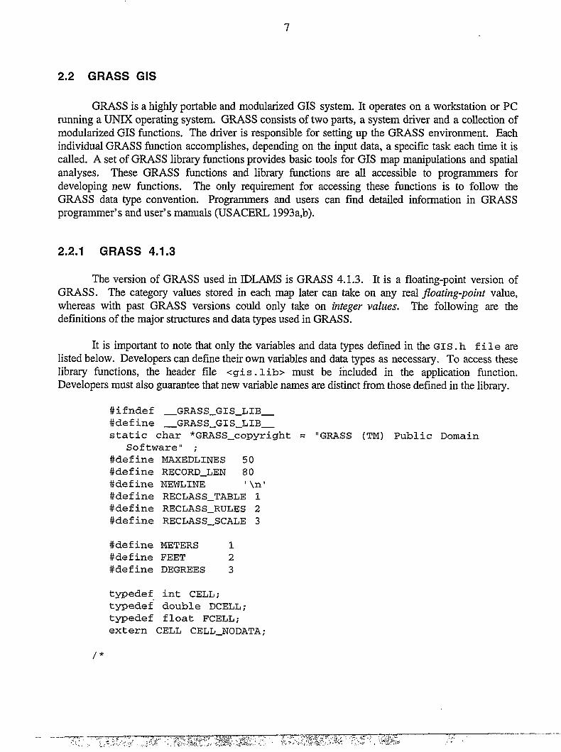
2.2 GRASS GIS
GRASS is a highly portable and modularized GIS system. It operates on a workstation or PCrunning a UNIX operating system. GRASS consists of two parts, a system driver and a collection ofmodularized GIS functions. The driver is responsible for setting up the GRASS environment. Eachindividual GRASS function accomplishes, depending on the input data, a specific task each time it iscalled. A set of GRASS library fimctions provides basic tools for GIS map manipulations and spatialanalyses. These GRASS functions and library functions are all accessible to programmers fordeveloping new functions. The only requirement for accessing these fimctions is to follow theGRASS data type convention. Programmers and users can find detailed information in GRASSprogrammer’s and user’s manuals (USACERL 1993a,b).
2.2.1 GRASS 4.1.3
The version of GRASS used in IDLAMS is GRASS 4.1.3. It is a floating-point version ofGRASS. The category values stored in each map later can take on any real floating-point value,whereas with past GRASS versions could only take on integer values. The following are thedefinitions of the major structures and data types used in GRASS.
It is important to note that only the vmiables and data types defiied in the GIS. h file are
listed below. Developers can define their own variables and data types as necessary. To access theselibrary functions, the header file <gis. 1 ib> must be included in the application function.Developers must also guarantee that new variable names are distinct from those defined in the library.
#if ndef _GRAS S_GI S_L IB_
#clefine _GRASS_GI S_LIB_
static char *GRASS_copyright = “GRASS (TM) Public DomainSoftware” ;
#define MAXEDLINES 50
#clefine RECORD_LEN 80#clefine NEWLINE ,\n,
#define RECLASS_TABLE 1
#define RECLASS_RULES 2
#define RECLASS_SCALE 3
#clefine METERS 1
#clefine FEET 2
#define DEGREES 3
typedef int CELL;
typedef” double DCELL;
typedef flost FCELL;
ext ern CELL CELL_NODATA;
/’

8
enum RASTER_MAP_TYPE{ CELL_TYPE = O,
FCELL_TYPE = 1,
DCELL_TYPE = 2
};doesn’ t
*/
typedef
#clefine
#define
#define
#define
#define
#define
#define
#define
#define
#define
compile on sun :( ?
int RASTER_MAP_TYPE;
CELL_TYPE O
FCELL_TYPE 1
DCELL_TYPE 2
PROJECTION_XY O
PROJECTION_UTM 1
PROJECTION_SP 2
PROJECTION_LL 3
PROJECTION_OTHER 99
PROJECTION_FILE “PROJ_INFO”
UNIT_FILE “PROJ_UNITS “
struct Cell_head
{int format ; /’ max numer of bytes per cell minus 1 ‘/int compressed ; /’ o = uncompressed, 1 = compressed, -1 pre3.-j */
int rows, Cols ; /’ number of rows and columns in the data ‘/int proj ; /’ Projection (see #defines above) ‘/int zone ; /’ Projection zone */double ew_res ; /’ East to West cell size */double ns_res; /* North to South cell size */double north; /’ coordinates of layer ‘/double south; double east;double west;
};
struct _Color_Rule_
{struct
{DCELL value;
unsigned char
} low, high;struct _Color_
red,grn,blu;
.Rule_ *next;struct _Color_Rule_ *prev;
};
struct _Color_Info_
{

9
struct _Color_Rule_ *rules;o int n_rules;
struct
{unsigned char *red;
unsigned char *grn;
unsigned char *blu;
unsigned char *set;
int nalloc;
int active;
} lookup;struct.t
DCELL *vals;
/’ pointers to color rules corresponding to the intervals
between vals */
struct _Color_Rule_ **rules;int nalloc;
int active;
} fp_lookup;
DCELL rein, max;
};
struct Colors
{int version; /* set by read_colors:DCELL shift;
int invert;
int is_float; /’ defined on floatingint null_set; /’ the colors for null
-I=old,l=new */
point raster data? */
are set? */unsigned char null_red, null_grn, null_blu;
int undef_set; /’ the colors for cells not in range are set?*/unsigned char undef_red, undef_grn, undef blu;—struct _Color_Info_ fixed, modular;DCELL cmin, crnax;
};
struct Reclass{
char name[50]; /* name of cell file being reclassed */char mapset[501 ; /’ mapset in which “name” is found */int type/* type of reclass */int num; /’ size of reclass table ‘/
CELL min,max; /’ table
CELL *table ;/* reclass};
struct FPReclass_table
range *;table */
{

10
DCELL dLow, dHigh; /* domain */DCELL rLow, rHigh; /’ range ‘/
};
/’ reclass structure from double to doubleused by r.recode to reclass between types:
int to double, float to int, ...
*/
struct FPReclass {
int defaultDRuleSet /* 1 if default domain rule set */
int defaultRRuleSet; /’ 1 if default range rule set ‘/
int infiniteLeftSet; /’ 1 if negative infinite interval rule
exists */
int infiniteRightSet; /’ 1 if positive infinite interval rule
exists */
int rRangeSet; /’ 1 if range (i.e. interval) is set ‘/int maxNofRules;
int nofRules;
DCELL defaultDMin, defaultDMax;
/*default domain minimum and maximum value ‘/
DCELL defaultRMin, defaultRMax;
/’ default range minimum and maximum value ‘/DCELL infiniteDLeft, infiniteDRight; * neg infinite rule */
DCELL infiniteRLeft, infiniteRRight; /* pos infinite rule */
DCELL dMin, dMax; /* minimum and maximum domain values inrules */DCELL rMin, rMax; /’ minimum and maximum range values in rules
*I
struct FPReclass_table *table;
};
struct Quant_table
{DCELL dLow, dHigh;
CELL CLOW, cHigh;
};

11
struct Quant
{
int truncate_only;
int round_only;
int defaultDRuleSet;
int defaultCRuleSet;
int infiniteLeftSet;
int infiniteRightSet;
int cRangeSet;
int maxNofRules;
int nofRules;
DCELL defaultDMin, defaultDMax;
CELL defaultCMin, defaultCMax;
DCELL infiniteDLeft, infiniteDRight;
CELL infiniteCLeft, infiniteCRight;
DCELL dMin, dMax;
CELL cMin, cMax;
struct Quant_table *table;struct
{DCELL *vals;
/* pointers to Quant rules corresponding to the intervals
between vals */struct Quant_table **rules;
int nalloc;
int active;
DCELL inf_dnin, inf_dmax;
CELL inf_min, inf_max;
/* all values smaller than inf_dmin become inf_min *//’ all values larger than inf_dmax become i.nf_max ‘//’ inf_min and/or i.nf_max can be NULL if there are no inf
rules */
} fp_lookup;
};
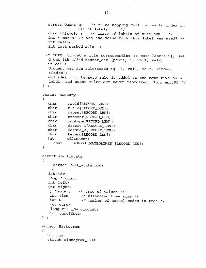
struct Categories
{CELL ncats; /* total number of categories */CELL num; /’ the highest cell values. Only exists
for backwards compatibility = (CELL)
max_fp_values in quant rules */char *title; /’ name of data layer ‘/char *fret; /* printf-like format to generate labels ‘/float ml; /’ Multiplication coefficient 1 ‘/float al; /* Addition coefficient 1 */float m2; /* Multiplication coefficient 2 */float a2; /* Addition coefficient 2 ‘/
12
struct Quant q; /’ rules mapping cell values to index inlist of labels ‘/
char **labels ; /* array of labels of size num ‘/int * marks; /* was the value with this label was used? ‘/int nalloc;
int last_marked_rule ;
/’ NOTE: to get a rule corresponding to cats.labels[i], useG_get_ith_c/f/d_raster_cat (peats, i, vail, va12)
it calls
G_quant_get_ith_rule (&catS->q, i, Vail, Valz, &inde~,&index) ;
and idex ==i, because rule is added at the same time as alabel, and quant rules are never reordered. Olga apr,95 */
};
struct History
{char mapid[RECORD_LEN] ;char title[RECORD_LEN] ;char mapset[RECORD_LEN] ;
char creator[RECORD_LEN] ;char maptype[RECORD_LEN] ;char datsrc_l [RECORD_LEN] ;char datsrc_2[RECORD_LEN] ;char keywrd[RECORD_LEN] ;int edlinecnt;
char edhist[MAXEDLINESl [RECORD_LENl ;
};
struct Cell_stats
{struct Cell_stats_node
{int idx;
1ong *count;int left;
int right;
} *node ; /’ tree of values ‘/int tlen ; /* allocated tree size *Iint N; /* number of actual nodes in tree */int curp;
long null_data_count;
int curoffset;
};
struct Histogram
{int num;
struct Histogram_list

13
{CELL cat;
long count;
] *list;
};
struct Range
{CELL rein;CELL max;
int first_time; /* whether or not range was updated ‘/
};
struct FPRange
{DCELL rein;
DCELL max;
int first_time; /’ whether or not range was updated ‘/
};
/*
** Structure for 1/0 of 3dview files (view.c)*/struct G_3dview{
char pgm_id[401; /* user-provided identifier */float from_to[21 [31; /’ eye position & lookat position ‘/float fov; /* field of view ‘/float twist; /’ right_hand rotation about from_to ‘/float exag; /* terrain elevation exageration */int mesh_freq, poly_freq; /* cells per grid line, cellsper polygon */
int display_type; /’ 1 fOr mesh, 2 for poly, 3 for both */int lightson, dozero, Colorgrid, shading, fringe, surfonly,
doavg; /*bools*/char grid_col[40], bg_col[40], other_col[40]; /’ colors */float lightpos[41; /’ casting, northing, height, I.O for
local 0.0 infin */float lightcol[31; /’ values between 0.0 to 1.0 for red,
grn, blu */
float ambient, shine;
struct Cell_head vwin;
};
struct Key_Value
{int nitems;
int nalloc;
char **key;
char **value;

14
};
struct Option /*{
char *key ; /’int type ; /*int required ; /*
int multiple ;. /*
char *options /*char *key_desc; /*
char *answer ; /*
char *clef ; /’char **answers ;
Structure that stores option info */
Key word used on command line */
Option type ‘/REQUIRED or OPTIONAL */Multiple entries OK */Approved values or range or NULL ‘/
String describing option */Option answer */Where original answer gets saved */
/’ Option answers (for multiple=YES)*/struct Option *next_opt ; /’ Pointer to next option struct ‘/char *gisprompt ; /’ Interactive prompt guidance ‘/int (*checker) () ; /’ Routine to check answer or NULL ‘/int count;
};
struct Flag /’ Structure that stores flag info ‘/
{char key ; /’ Key charchar answer ; /’ Storeschar *description ; /*struct Flag *next_flag ;
};
/’ for G_parsero ‘/#define TYPE_INTEGER
#define TYPE_DOUBLE
#define TYPE_STRING
#define YES
#define NO
#ifndef FILE
#include <stdio.h>
#endif
#include “gisdefs.h”
#include “datetime.h”#include “site.ht’
struct TimeStamp {
DateTime dt[21;
int count;
};/*_GRASS_GIS_LIB_* /
used on command line */
flag state: 0/1 */String describing flag meaning ‘/
/’ Pointer to next flag struct ‘/
1
2
3
10
/* two datetimes ‘/

15
2.2.2 Programming Library
The GISLibra~is tiepfim~progrting tibr~provided with tie GWSS GIS system.This library contains functions needed to access the map database. More than a hundred GRASSlibrary functions are available in the GIS library. Developers can use them anywhere in theirapplications as long as the rules specified in the GRASS Programmer’s Manual and the User’sReference Manual are followed. A detailed explanation of each function is beyond the scope of thismanual. Users and programmers are advised(USACERL 1993a,b).
2.2.3 Segmentation Technique
t; see the relevant GRASS manu-ds and doc~entation
Although detailed explanations on usage of all of the GRASS functions are provided in theGRASS Programmer’s Manual, a few tips on the map segmentation technique might be helpfil toprogrammers, because this technique must be used when a large map layer and multiple map rows areto be manipulated in a model. If the map segmentation technique must be used in a model, attentionshould be given to the following:
1.
2.
3.
4.
5.
6.
The category data must be read as character strings and then converted tocorresponding integer or floating-point datrq
The types of variables designated to receive the category values must be defined asdouble precision if the map to be read is a floating-point map;
The segment buffer must be flushed before the segment fde can be reopened;
The segment buffer must be flushed before the termination of the function;
The program must implement code to remove the segment fde created, thewill not remove it automatically;
library
The addresses of the receiving variables (instead of the variables themselves) mustbe used in reading segmentation fdes.
Additional information concerning the map segmentation technique is provided in later sectionsof this manual. For more details on the map segmentation technique, please see the GRASSProgrammer’s Manual (USACERL 1993a).
2.3 IDLAMS Environment
IDLAMS is built on the GRASS GIS environment. In order to run lllLAMS and GRASS GISfi.mctions, some environment variables must be set at the start up of IDLAMS. An I13LAMS runcontrol file . idl amsrc file is produced when IDLAMS is installed. All of the environmentalvariables necessary to run IDLAMS are defined in this file. Table 3 is an example of the . i dl ams rcfile.

16
Table 3 Variables Defined in . idlamsrc File
GISBASE : /home/grass4.l
GISDBASE : /dataOLOCATION_NAME: riley
MAPSET: DLMS
PAINTER: ppm
DIGITIZER: none
MONITOR: xl
Each time an IDLAMS section starts, the driver program (l) reads the parameters, (2) starts atext fomatinput section fortieuser tomAechmges ifso desired, and(3) exports them as UNIXenvironment variables. In addition, the user must also be prevented from starting another session,which could disturb the integrity of the GIS database. These two important problems are solved inIDLAMS by the function grass. tel. The IDLAMS system calls this fhnction when the user clicksthe CONTINUE button in the first screen. It then picks up the process number, PID, sets up GRASSenvironment variables, and exports them to the UNIX environment. The parameters set by thefunction grass are listed in Table 4.
Table 4 Variables Defined by Function grass
PATH (GISDBASE ): /dataO
LOCATION_NAME: ri 1ey
MAPSET : IDLAMS
PAINTER: ppm
DIGITIZER: none
GISLOCK: pidMONITOR: xlXDRIVER_LEFT : 650XDRIVER_TOP: 5
The last two items are optional for running GRASS. The purpose of setting these parametersis to define the position of the GRASS monitor.
2.4 Data Directories and Management
IDLAMS works directly with GRASS4. 1 GIS maps in a mapset named IDLAMS. The usermust set up this mapset before running IDLAMS. Programmers can find the data structure of GRASSmapsets in the GRASS4. 1 Programmer’s Manual (USACERL 1993a).

17
Users can import maps in formats other than GRASS GIS either via an ASCII fde or directly,by converting the import maps into GRASS format via format converting utility functions (if suchfunctions are available). Similar functions also exist in other GIS packages. In addition, the user canalso find useful tools for map format conversion from the GRASS web page at:
http: //www. cecer. army. roil/grass/
Many GRASS GIS system users have made contributions to this web site.
2.5 GNUPLOT
The IDLAMS technology’s scenario evaluation model utilizes the GNUPLOT software(Williams and Kelley 1993). Within IDLAMS, GNUPLOT is used to produce and display graphics,specifically bar charts, as visual displays to the user. Several bar charts are available to the user as arepresentation of functionality.
It is important to clari~ that the information displayed in the IDLAMS scenario evaluationGNUPLOT bar charts serves only as a representation of the functionality of the GNUPLOT software,linked with single-attribute and multiple-attribute utility finctions that are based upon the objectiveswithin the scope of a larger decision-making process. The inputs and outputs are not meaningfulquantities (values) and currently serve only as placeholders. A programmer, system administrator, oruser who is accessing and running the scenario evaluation model should observe how it operates andthe functionality that it provides, rather than attempting to actually use the scenario evaluation inmaking any decision on the land management alternatives under consideration through IDLAMS.Within IDLAMS, GNUPLOT is utilized only for displaying bar charts for the purposes described inthe previous section, In summary:
“GNUPLOT is a command-line driven interactive function plotting utility for UNIX,MSDOS, and VMS platforms. The software is copyrighted but freely distributed (i.e., youdon’t have to pay for it). It was originally intended as a graphical program which wouldallow scientists and students to visualize mathematical functions and data. GNUPLOThandles both curves (2 dimensions) and surfaces (3 dimensions). Surfaces can be plotted asa mesh fitting the specified fimction, floating in the 3-d coordinate space, or as a contour ploton the x-y plane. For 2-d plots, there are also many plot styles, including lines, points, lineswith points, error bars, and impulses (crude bar graphs). Graphs may be labeled witharbitrary labels and arrows, axes labels, a title, date and time, and a key. The interfaceincludes command-line editing and history on most platforms.”(http://science.nas.nasa.gov/people/woo/ gnuplot_info.html 1998)

18
3 VEGETATION DYNAMICS MODEL
The vegetation dynamics model is the central component of IDLAMS. It takes as input anASCII text fde containing information on the run inputs and environment variables, plus directorystructure (e.g., resolution, geographic region). The output is a GRASS raster map layer.
3.1 Input File
The input file, which contains all information necessary for the model to run a simulation, canbe constructed with any text editor or interface. Figure 3 shows an example of an input file for thevegetation dynamics model.
Line Description
1.
2.
3.
4.
5.
6.
7.
8.
9.
10.
11.
1992 2007
trn. dist
landcover_input_map
himgt .medtrn. 500m. seen
01345
500000
500
500
50000
2
4 15
start ing/ ending year
training map
1andcover map
output map
reclass categories
maneuver impact mi 1es
erosion control planting (at)
native planting (ac )
prescribed burning (at)
successional change (forest)
successional change (early, late)
Figure 3 Sample Input for the Vegetation Dynamics Model
The first line of the input fde consists of two items. The first item is the starting year of thesimulation; the second item is the ending year. The second line provides the name of the trainingintensity distribution map. This map contains a floating-point, normalized training intensity value ineach pixel and is generated for installations by using methodology established through the Land BasedCarrying Capacity Program (Guertin, Rewerts, and Dubois 1997). The third line item in the input fileis the initial landcover map, followed on the fourth line by the name of the desired output map. Thefifth line of the input file consists of five items, which are the categories the user selects to reclass theoriginal categories in the input landcover map. These five new categories are as follows: (1) Forest,(2) Forest/Shrub/Grass Mixture, (3) Disturbed (training darnage), (4) Early Successional, and (5) LateSuccessional, respectively.
The sixth input line is the Maneuver Impact Miles (MIMs), a measure of the training loadcalculated as part of the Army Training and Testing Area Carrying Capacity (AITACC) program(Concepts Analysis Agency 1996). The seventh, eighth, and ninth lines of the input file are theacreages of the land management practices (i.e., erosion control planting, native planting, andprescribed burning, respectively). The tenth and eleventh input lines describe the vegetationsuccession parameters. Of the three parameters defining vegetation succession, the first is the

19
probability (in percent) that a grass pixel changes to forest (line 10). The second and third are thenumber of years it takes for early successional to change into late successional and for damaged tochange into early successional grass categories (line 11). The command line format for calling thevegetation dynamics model is:
r.veg. change input_f ile_name
The input file is built by a series of GUI screens to guide the user in entering necessary inputdata. Cost functions and a display screen have been implemented in the system to dynamicallycalculate and display the costs of the user-selected land management activities. The regional costestimates of land management practices can be found in Gebhart and Warren (1995). These costs areheld in a fde named cost. t c1 in the IDLAMS main directory. The user and/or programmer canchange these numbers by using any text editor. The cost of each activity and the sum of the individualcosts are displayed dynamically on the same screen simultaneously. The input of Maneuver ImpactMiles (MINIs) provides a measure of the land training impact and is consistent with the trend ofcarrying capacity studies in the current efforts on Army Training and Testing Area Carrying Capacity(ATTACC) and Integrated Training Area Management (lTAM) research supported by the Army. Forfurther information concerning these programs, contact the Army Environmental Center (AEC) atAberdeen Proving Ground, Maryland, the Office of the Deputy Chief of Staff for Operations and Plans(ODCSOPS), and the Assistant Secretary of the Army Installations Logistics and Environment (ASA(ILE)) at Headquarters, Department of the Army, Washington, D.C.
3.2 Model Execution
Upon execution of the vegetation dynamics model, the initial age status of the landcover isdetermined by randomly assigning ages within different landcover types in the user-provided initiallandcover map. This is done because the number of years each pixel has been in its current landcoverclass is unknown. Upon execution of the vegetation dynamics model, these pixels then proceedthrough succession into new landcover classes, based on what the user has selected as the timeintervals between each successional stage. If no land management or training takes place in asimulation, vegetation categories simply change via succession at the rates specified by the user.However, as described below, land management and training activities affect succession in variousways. Figures 4 through 8 show flow diagrams for the vegetation dynamics model and its functionalcomponents.
The user-specified acreage (number of acres) of prescribed burning is then applied by selectinga random cell and allowing the “burning” to spread from there to surrounding areas. However, valleyareas defined by a valleydef map are not burned by the prescribed burning. Valleydef is an internalIDLAMS function that identifies the valley boundaries for terrain areas with woody draws (thesedraws shelter the enclosed vegetation from fires). These draws are identified from processing digitalterrain maps (DTMs). The prescribed burning function could be altered to take burning rotation planmaps as input if desired. The prescribed burning will alter landcover classes by (1) speeding up earlysuccessional to late successional and damaged to early successional if the current pixel in the map isearly succession or damaged category, respectively, and (2) preventing late succession fromsucceeding into shrub or forest. The landcover category of a given pixel is then checked, and naturalsuccession takes place if the category of the cell as well as its surrounding pixels meet successioncriteria.

20
Read in Input from .projecfnane File
I Initialize the Area I
I Calculate the MIMs Distribution I
b Calculate the Damage DistributionI
I Category or Age Change caused by Prescribed Fire .—> Prescribed Burn Function
I Categoy Change caused by Natural Vegetation Succession
+I I
(see Figure 4)
Vegetation SuccessionFunction
(see Figure 5)
I Make the Category Changes if Damage Criteria are Met l-+ Training FunctionI I
4
(see Figure 6)
Make Category Changes due to Planting ~ plafltin9 Function(see Figure 7)
I
Figure 4 Flow Diagram of Vegetation Dynamics Model Main Function

21
Generate Random Numbers i and j
mClump the Area for All Cells around Cell CU until the
Area Is Equal to the Number of Acres to Be Burned
‘es+=Yes
Chang etoLateSuccessional
I
No
& No
vYes
Change the Number of Years Required for Vegetation
to Change from Early to Late Successional CategoryE
‘e-Figure 5 Flow Diagram of Prescribed Burning Function
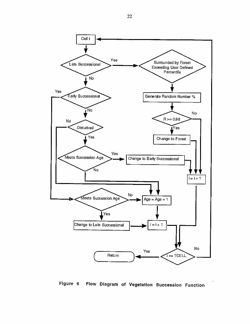
22
I Cell i 1+
‘eNo
-N&+
Yes
Generde Random Number Y. I
e’& 1
1
i= i+l I
+Yes
+
Change to Late Successional [+=q
l?roCE3- “ ‘2I >= TCE LL
Figure 6 Flow Diagram of Vegetation Succession Function

23
MIMs * C = Acres
MIMs * C * TRj= Di
Atot
i
Sort Cells in Order from Highest Di to Lowest Di
Dj * MIMs = DMIMj
(MIMs Put on Cell i)
i-1
SDMIM =z
DMIMj
j=l
No
Yes
dim+
— Change the Category of Cell to Damaged
Figure 7 Flow Diagram of Training Function

24
I Clump Damaged Areas
I List All Areas that Are Greater than 15 Acres
Randotdy Select an Area from the Previously Created List
Plant This Area with Given Type of Grass
&
No *T
Pick a New Area in the List
Yes
IPartly Plant the Last Patch

25
Next, the training impact is distributed onto the landcover map, on the basis of the ManeuverImpact Miles and the training intensity distribution map. The former is the equivalent of AbrahmsMIA1 main battle tank maneuver tracking miles on.an installation caused by all training activities, andthe latter is a 0-1 scale normalized training intensity (Concepts Analysis Agency 1996). The number ofIvDMsapplied to each pixel is determined by multiplying the average MINIs for the whole installationby the training intensity value of the pixel. The number of MIMs applied to each pixel is thenconverted to Mea by multiplying MIMs by the width of the footprint of the MIA1 tank. Thisrepresents the area of the pixel that receives training impact. Thus, the training impact is directly relatedto the training intensity.
A comparison is made between the area affected by training impact and the size of the cell. Foreach pixel, if the total area affected by training is less than 40% of the pixel size and the vegetationcategory of the pixel is early successional grasslands, the pixel remains early successional.Conversely, if the percent affected exceeds 40%, the pixel reverts to damaged grasslands. This 40%cut-off is a best estimate and can be changed if research supports a better estimate in the future.Similarly, the same cut-off rule is applied to pixels representing late successional grasslands, exceptthat the affected area must be greater than or equal to 60% of the pixel for a later successional categoryto become a damaged vegetation category.
Finally, the planting function (erosion control or native species) is applied. This is done byfirst aggregating or “clumping” (r. clump in GRASS) the areas of damaged grasslands and thenrandomly planting only on those damaged areas that exceed 15 acres in size.
The vegetationr .veg. change. TheGRASS subdirectory:
dynamics model is written as a standard GRASS function, namedsource code is placed, as are all other GRASS main raster functions, in the
src/raster/r. veg. change /cmd/
The vegetationdynamicsmodel consistsofsevenfunctions:
main. c
assign_ init_age. c
change_cat. ccheck_change2 forest. c
cseg_get .c,dseg_get .c
planting. c
prescribed_f ire. c
Functionmain. c servesas a driverto (1)read input parameters and maps, (2) initialize mapsegmentation files for input and temporary maps, (3) call other functions to perform vegetationsimulation calculations under given training intensity and land management activities, and (4) producean output vegetation map at the end of the simulation. Function as sign_ini t_age. c randomlyassigns initial age or a representation of the number of years a cell has been in a particular landcovercategory in the input landcover map. Function change_cat. c is designated to change the age or thecategory of the current category if the current category meets conditions set forth for natural successioncategory change. Vegetation categories are all defined in the header fde veg. h. Functions

26
ass ign_ini t_age. c,change_cat. c,and theheaderfileveg. h must be modifiedifthecurrent
classificationcategoriesneed to be changed. Table 5 shows the vegetation categories defined inveg. h.
Table 5 Vegetation
#define C_NODATA
#clefine C_FOREST
#define C_SHRUB
Categories Defined in Header File veg. h
o /*1 /*
2 /’#define C_DISTURBED 3 /’#define C_EARLY 4 /*#clefine C_LATE 5 /*#clefine C_TURF 6 /’#define C_NATIVE 7 /’
Nodata cell category
Forest Category
Shrub Category
Training Damaged Category
Early Successional Category
Late Successional Category
Planted Turflike/Erosion Control
Planted Native Grass
*/
*I
*/
*/
*/
*/
Grass *I
*/
Amapsegmentation technique has been employed inthis vegetation dynamics model. Withthis technique,maps are partitioned into block data inaforrnat that is readable and writeableas ifthewhole map were stored in computer memory, whereas in fact only a fraction of the map is actuallystored inthememory. This technique allows the model to swap only part of a huge map into thecomputer memory at a time and perform manipulations so that the model can handle any size map atany desired level of resolution. This use of map segmentation makes IDLAMS more applicable toinstallations with large data sets.
The map segmentation technique has been implemented as part of the GRASS Iibray function.Programmers can access these functions by including the <s eg. h> header file in the applicationfunction. The call to these functions is the same as to any other library function. However, a fewextra parameters must be defined. In order to make the segmentation library function compatible withthe floating-point map, a modified version of cs eg_get. c and a double-precision floating-pointversion of this function dseg_get. c have to be made. Table 6 shows the parameters defined in theheader file veg. h for the map segmentation technique to function. A complete list and detailedexplanation of the segmentation functions and their required variables can be found in the GRASSProgrammer’s Manual (USACERL 1993a).
Finally, the function plant ing. c assigns a given amount of grass to be planted withinclumped damaged areas. Also, the fimction pres cribed_f ire. c burns a given area clumpedaround a randomly selected cell. More information about the development of the vegetation dynamicsmodel can be found in the IDLAMS Final Report.

27
Table 6 Definitions of Variables for Map Segmentation Functions
/* Define the segmentation variables and assign them values */
#define SROWS 9 /* Number of rows in the segment ‘/
/’ file ‘/
#define SCOLS 13 /’ Number of columns in the segment*//’ file. SROW and SCOL together */
/* define the format of the segment ‘/
/* file. */
#define SWAP_13LOCK 512
/* SWAP_BLOCK defines the size ‘/
/* in byte of the portion of the map *//* retained in memory space ‘/
int trnmap_fd, lndmap_fd;
int age_fd, fireafect_fd;
int temp_fd, valydef_fd;
/’ Define the file descriptors for the *//’ segmentation files used to
/* segment the maps to be opened.
char *lndseg_file, *trnseg_file;
char *ageseg_file, *fireafect_file;
char *tempseg_file, *valydef_file;
/* Define the segmentation files */
int flen, ilen; /* The lengths of floating point ‘/
/* map cell FCELL and the integer
/’ map cell CELL respectively
SEGMENT trnmap_seg, lndmap_seg;/* Define segmentation structures
/* for the training intensity map
/* and the land cover map.
SEGMENT fireafect_seg, age_seg;
*/
*/
*/
*/
*I*/*/
/* Define segmentation structures to ‘/
/*
/’
SEGMENT valy_seg;
/’
/*
/’
SEGMENT temp_seg;
store fire affect and vegetation */
succession criterion */
Define segmentation structure */
forest spread constraint valley */
def map. ‘/
/* Define segmentation structures */
/’ for a working segmentation file ‘/

28
4 WILDLIFE HABITAT SUBMODELS
All wildlife habitat submodels are written in UNIX Bourne shell scripts using GRASSfunctions. If desired, sites can develop these models in other GIS modeling languages (e.g.,ARC/INFO, GRID). The inputs of these models are directly obtained from the Tc~k graphical userinterface. A habitat suitability map is calculated for each wildlife species. The calculations areperformed on the basis of the current Iandcover map or the output map of the vegetation successionmodel and other maps, such as foodplots, soil texture, and nesting area, where applicable. GRASSfunctions r.mapcalc, r. buffer, r.clump, r.reclass, r. stats, and r.neighbors areemployed in the calculation. In addition, an internal function, c lumpz c las ses, has been developedin C language to provide a tool for screening out aggregated areas or “clumps” having a contiguousarea less than the user-specified size.
The command line format of function clumpz! class is:
clump2classes pl p2 p3 p4
where
P’ = r. clump map statistic output (generated using r.s tats);
P’ = user-desired minimum contiguous nesting area size;
P’ = 10,000, a conversion for hectares; and
P4 = output file (this fde is used to pass through r. rec 1ass to reclass the r. clump resultmap into only those meeting the contiguous area criteria).
There are five different wildlife habitat simulation submodels in the current Fort Riley LDLAMSsystem. They are as follows: (1) northern bobwhite (Colinus virginianus), (2) Henslow’s sparrow(Ammodramus hensknvii), (3) greater prairie chicken (Tympanuchus cupido), (4) prairie mole cricket(Grylhu’pa ma@-), and (5) regal fritillary (S’peyeria idalia). Again, users can develop their ownsubmodel(s) as appropriate for specific ecosystems or regions. More information about thedevelopment of the wildlife submodel can be found in the IDLAMS Final Report.

29
5 EROSION SUBMODEL
The soil erosion submodel in lDLAMS calculates the soil erosion status by dividing the resultof the Revised Universal Soil Loss Equation (RUSLE) (Wischrneier and Smith 1978) by soil erosiontolerance, T, factors. The soil erosion model is also implemented in Boume shell programminglanguage by using the GRASS function r. mapcalc. User inputs for this model are (1) K factormap, (2) LS factor map, (3) T factor map, and (4) C factor map. The C factor map is the only factorthat will change on the basis of different vegetation dynamics simulations. The user is provided with atable for manually reclassifying Iandcover to C factor values. For sites implementing the LandCondition Trend Analysis (LCTA), data can be used to reclass landcover into C factor values. Again,sites wishing to implement alternative erosion or watershed models may do so by ensuring that thesemodels can take ASCII kmdcover arrays as input. More information about the development of theerosion submodel can be found in the IDLAMS Final Report.

30
6 SCENARIO EVALUATION MODEL
A complete description of the decision-making process built into IDLAMS is beyond the scopeof this document, and is covered in depth in the IDLAMS Final Report. The following briefdescription is meant only as an introduction to the workings of the scenario evaluation model and adiscussion of topics of interest to programmers.
6.1
naturalseveral
IDLAMS Succession Models
A fundamental theory of operation of the IDLAMS environment involves the simulation ofvegetation succession over time for a given area of land. This simulation can be performed inways, to provide different levels of detail and approximation needed in differ~nt IDLAMS-.
modules. The vegetation dynamics model executes a cell-by-cell succession simulation. The scenarioevaluation model works directly with the result maps from that cell-by-cell simulation. It can alsoexecute a bulk succession simulation and process the more general results for trends. The successionstages used by both the cell-by-cell model and the bulk model are illustrated in Figure 9.

31
Damaged
v
\shrlJb
Figure 9 Successional Transitions in the Life of a Landcover Map Cell
The cell-by-cell model, which predicts succession on the basis of each cell’s neighbors, is veryslow but provides spatial detail regarding what landcover type appears, and where it appears, in a site.Statistics gathered on the final resultant map (using r.stats) are used to score that scenario’s usefulness.Figure 10 illustrates a typical landcover map.

32
Figure 10 Landcover and Training Areas Map
The bulk statistics model gathers statistics at the start of the simulation, using these values onlyto predict the successive Markov state probabilities. In this way, it executes many times faster but atthe cost of true spatial detail associated with the resultant map. The bulk model is called quickly anduses the scenario evaluation model to score different land management practices.
6.2 Decision-Making Strategy
Scenario Evaluation
The decision-making process involves defining, examining, and comparing the effects of landmanagement practices implemented at a given military installation. Any given collection of parametersand a time period over which they are valid and operate is referred to as a scenario. The decision-making process begins by evaluating each scenario result through a systematic process of identifyingland use objectives, assigning objective measures and objective weights, and collecting theseobjectives, measures, and weights into single- and multiple-attribute utility functions that can bemathematically optimized.

33
Scenario Comparison
The parameters selected and the values used to represent them were gathered during a stagedworkshop, where experienced personnel were interviewed through a system of interrelated andcounter-related questions to identi@ and compare the objectives and establish their measures andranked weights (Keeney 1992). The objectives, measures, and weights were combined into single-attribute utility functions, yielding a multiple-attribute utility function score for each scenario. Theutility score values produced are concatenated into a script command line call to GNU software’sGNUPLOT (Williams and Kelley 1993) for visual display to the user (see Figure 11).
.N wf”ii3 e’!$li-$$twfk$a d-i% Wtw?i’ ““
-T
Figure 11 Typical Single-Attribute Utility Functions Graph
Each scenario has a utility (or composite functional usefulness) assigned to it, so themanagement practices modeled by the parameter choice can be compared.
6.3 Algorithm and Data Representation
The environmental objectives are represented by simple category values. Each objective hasassociated with it a series of formal measures and weights for those measures, each represented by anumeric value. These measures are defined through interviews with the user(s) and are combined intosimple algebraic (in this case) utility functions of the form
u(x) =kll u1l (x111,x112,x113) +k12 u12 (x12) +k13 u13 (x131,x132,x133) +k21 u21 (x21) +k22 u22 (x221,x222,x223) +

34
k23 u23 (x23) +
k24 u24 (x24) +
k25 u25(P251 x251 + P252 x252 + P253 x253 + P254 x254)
The evaluationof thesefunctionsintoutilityscoresis straightforward.The collectionof
scenariostatisticsuses only smallamounts of memory, in comparison with storingentirelandcover
maps. Thestatisticsarestoredasdynamic arraysrepresentingsparsematrices.In thisway, memory
is used efficiently and allows reasonably large problems to be addressed.
6.4 Algorithm Implementation
The decision-making process involves evaluating a series of utility functions.functions were first developed and modeled in a spreadsheet environment, wheremathematically validated. The utility functions were then coded in C and UNIX scripts and
All developed code compiles and executes by using standard ANSI C
The utilitythey werevalidated.
compilers.Subdirectories for all the required codes are listed, and the IDLAMS Installation Manual describes howthey are set up for the operation.
6.5 User Input Required
The decision making begins by prompting the user for parameter values through a Tc~k“expect” interface. The “expect” calls capture the input the user is typing in widget fields and storethem in local environment variables. The bulk of these values have preprogrammed defaults, but inorder to execute successfully, the user must select the names of several GIS maps as well. Theindividual map names are captured and stored as global variables.
6.6 Model Output Produced
The output from the scenario evaluation model is a report generated and opened for reviewduring the IDLAMS session (see Figure 12). The report output screen is produced by a Tcl/Tk script.
‘i\ Thatotal.vakxi’h%ru$ilftyftii’m’ ;s0;5?5 ‘ ‘, “ .’ ‘,: $. ,,’~
,.. , ., ...‘ . ..., ,, .,, ,:,:. , /,, -. .,,. .,, ,, ’;’ .’,
Figure 12 Typical Evaluation Model Statistics Report

35
7 REFERENCES
Concepts Analysis Agency, 1996, Evaluation of Land Value Study (ELVS), U.S. Army ConceptsAnalysis Agency, Study Report CAA-SR-96-5, Bethesda, Md.
Gebhart, D.L., and S.D. Warren, 1995, Regional Cost Estimates for Rehabilitation and MaintenancePractices on Army Training Lands, USACERL Technical Report 96/02, Oct.
Guertin, P.J., C.C. Rewerts, and P.C. Dubois, 1997, Training Use Distribution Modeling, U.S.Army Construction Engineering Research Laboratories, Champaign, Ill., CERL Technical Note 97-XXX, Sept., (in preparation), 6 pp.
Internet address: http://science.nas. nma.gov/people/woo/gnuplot_info.htti 1998, June 5, 1998.
Keeney, R., 1992, Value-Focused Thinking, Harvard University Press, Cambridge, Mass.
Ousterhout, J., 1995, TcVI’k Installation and Documentation Directory, University of California atBerkeley, ouster @cs.berkeley.edu.
USACERL: See U.S. Army Corps of Engineers, Construction Engineering Research Laboratories.
U.S. Army Corps of Engineers, Construction Engineering Research Laboratories (USACERL),1993a, Geographic Resources Analysis Support System (GRASS), Version 4.1, Programmer’sManual, M. Shapiro et. al., Champaign, Ill.
U.S. Army Corps of Engineers, Construction1993b, Geographic Resources A.@ysis SupportManual, Champaign, Ill.
Engineering Research Laboratories (USACERL),System (GRASS), Version 4.1, User’s Reference
Williams, T., and C. Kelley, 1993, GNUPLOT, An Interactive Plotting Program, Version 3.5, ~gmmlot-reauest @dartmouth.edu.
Wischmeier, W.H., and D.D. Smith, 1978, Predicting Rainfall Erosion Losses — A Guide toConservation Planning, U.S. Department of Agriculture, Agricultural Handbook No. 537.