integrated force method versus displacement methodfor ... · integrated force method versus...
TRANSCRIPT

NASATechnical
Paper2937
February 1990
.... + _
_ . • -- ...... -
= . • . _,
__ H +++2._ .... - ........
+ ." 2 J -= ='+ "
d
+ :;:..:+_+................++= = =-. _-_
-2_+g -+ ...... = . _ +
Integrated Force Method
Versus DisplacementMethod.............for .........Finite"" ._
Element Analysis
Surya N. Patnaik,
Laszlo Berke, and
Richard H. GaUagher
unclas
H 6k
https://ntrs.nasa.gov/search.jsp?R=19900008765 2018-05-28T13:12:34+00:00Z

L

NASATechnical
Paper2937
1990
tU/L. ANational Aeronautics andSpace Administration
Office of Management
Scientific and TechnicalInformation Division
Integrated Force Method
Versus DisplacementMethod for Finite
Element Analysis
Surya N. Patnaikand Laszlo Berke
Lewis Research Center
Cleveland, Ohio
Richard H. Gallagher
Clarkson University
Potsdam, New York


Summary
A novel formulation termed the "integrated force method"
(IFM) has been developed in recent years for analyzingstructures. In this method all the internal forces are taken as
independent variables, and the system equilibrium equations
(EE'S) are integrated with the global compatibility conditions
(cc's) to form the governing set of equations. In IFM the cc'sare obtained from the strain formulation of St. Venant, and
no choices of redundant load systems have to be made, in
contrast to the standard force method (SFM). This property of
IFM allows the generation of the governing equation to be
automated straightforwardly, as it is in the popular stiffness
method (sM). In this report I_ and su are compared relative
to the structure of their respective equations, their conditioning,
required solution methods, overaI1 computational require-
ments, and convergence properties as these factors influence
the accuracy of the results. Overall this new version of theforce method produces more accurate results than the stiffness
method for comparable computational cost.
Introduction
Solutions of structural mechanics problems must satisfy the
appropriate equilibrium equations (dE'S) and compatibility
conditions (cc's) in addition to the constitutive relations (cg's)
describing material behavior. In what order, and to what
extent, these three requirements are satisfied defines the
method of analysis and the quality of the solution. This reportconcentrates on the relative roles of EE'S and cc's in structural
analysis. The constitutive relations, combinations of proper
mathematical models and experimental results, here are
presumed to be available in valid forms, even though that is
not always the case.This report compares the two most fundamental approaches
to analyzing finite element models of structures: the force
method and the displacement method. The details of these two
methods, and their relative characteristics, were discussed
intensively three decades ago during the early evolution of
computer-automated structural analysis. As is well known, the
displacement method won out for computer automation in the
form of the stiffness method (SM). As briefly discussed herein,the force method available at that time was based on the
concept of redundant selections. It was the result of approaches
developed for hand calculation in the precomputer era and
proved inconvenient to automate and computationally more
costly than the displacement method.A new version of the force method, described herein and
compared with the displacement method, was introduced in
references 1 and 2 and termed "the integrated force method"
(WM). It is shown in a comparison with the early force methods
(ref. 1) that the IFM makes automation as convenient as it is
with the displacement method and yet retains the known
potential for superior stress-field accuracy of finite elementmodels that is associated with force method solution
techniques. Furthermore IFM provides a convenient way toenforce an additional constraint on a finite element model of
a continuum, namely strain compatibility at the interelement
boundaries. This constraint, usually not satisfied, appears to
result in significant improvement in accuracy.
The IFM integrates the system EE'S and the global cc's in
a fashion paralleling approaches in continuum mechanics (e.g.,
the Beltrami-Micheli formulation of elasticity (ref. 3)). The
iFra is a natural way of integrating the use of EE'S and cc's.
In contrast, the classical force method (refs. 4 and 5) (referred
to in this report as "the standard force method" (s_)),
satisfies the cc's through the somewhat ad hoc and artificial
concept of selected redundant internal forces. Consequently,
IFM provides a strong motivation to reexamine the relative
merits of the force and displacement methods within thecontext of the finite element idealization. A project was begun
for that purpose, and its results are presented in this report.
The primary conclusions of the comparison are as follows:
(1) The i_,i inherits from the SFM the ability to operate
directly on stress parameters and thus to provide potentially
more accurate stress results than does the displacementmethod.
(2) The IFM equations for finite element discrete analysis
form a well-conditioned system.
(3) Discrete analysis solutions (stresses and displacements)
obtained by IFM tend to converge to correct solutions more
rapidly, in terms of the number of elements, than the same
solution generated by the stiffness method.
(4) Examples indicate that certain problems can be solved
by IFM in less computation time than by SM.(5) Initial deformation problems are more elegantly treated
by ivra than by SM.
This research indicated that with further development the IFM
can become a robust and versatile analysis formulation and
a viable alternative to the popular displacement method. The
nature of its equations makes the IFrd an attractive candidate

fortheinclusionofinitialdeformationsfromvarioussources(e.g.,manufacturingtolerancesorsignificantthermaleffectsandmaterialnonlinearities).
Historical Background
It is of some interest to briefly revisit the historical evolution
of the various formulations for solving structural mechanics
problems, and specifically that of the displacement and forcemethods.
The concepts of equilibrium of forces and compatibility of
deformations are fundamental to analysis methods for solving
problems in structural mechanics. There was a certain degree
of asymmetry in the developmen t and utilization of these twoconcepts, as described here.
Early on, when hand calculations were used, the forcemethod was favored because it resulted in a much smaller set
of simultaneous equations, usually related to the redundant
forces in a roof or bridge truss, than did the displacementmethod. With the appearance of computers that consideration
lost its importance in favor of ease of automation and low
computational cost.
Equilibrium can be viewed as a more fundamental concept
than compatibility. Engineers have a feel for it, perhaps
because it was practiced consciously or subconsciously by the
first builders of primitive human habitats in the dim past of
human evolution, by the architects of magnificent edifices of
biblical empires, and then by the builders of cathedrals, whofaced the intricate equilibrium problems of Roman and Gothic
arches and domes. If equilibrium was violated, or was
precarious, the construction responded by tumbling down.
Recall that the mere blast of horns is supposed to have caused
certain wails in Jericho to collapse in a much simpler era of
structural analysis and construction practices.
The point is that equilibrium is such a natural concept thatgood engineers have alwayshad a feel for it, and it was the
guidance for most early achievements. In contrast, the more
sophisticated and basically mathematical concept of compati-
bility certainly was not central to the worries of these earlybuilders and architects; it was n0t even known until math-
ematicians defined it only a century ago.
Rational principles to define the equilibrium conditions of
mechanical forces had an early start with the work of
Archimedes (287-212 B.C.) on levers and pulleys. A couple
of millennia passed before the upsurge of rational scientific
thought during the Renaissance brought about further
significant theoretical developments. With the efforts of many
scientists during the centuries that followed, the concepts of
equilibrium and compatibility were finally developed in forms
that eventually became useful for design calculations. Because
it helps to understand how the current computer-automated
analysis practices evolved, the history of this development is
briefly reviewed.
2
Renaissance geniuses like Leonardo da Vinci (1452-1519)
and Gallileo (1564-1642) used the concept of equilibrium in
their work, but even Gallileo, a professor of mathematics, did
not possess the proper mathematical language to express the
fundamental laws governing equilibrium in a continuum. That
had to wait until the introduction of that language (i.e.,
calculus) by Newton (1642-1726) and Leibnitz (1636-1716).
This new mathematical toot attracted many of the great
minds of the Age of Enlightenment, who finally were in the
possession of mathematical language to formulate correct lawsof physics. Elasticity was introduced as a branch of
mathematics, rich in the possible applications of the excitingnew tool of calculus. The Bernoulli brothers and Euler were
enthusiastic early proponents of the use of calculus in
mechanics. Following in their footsteps many great scientistscontributed to the early developments in eiasticity_ A
fundamental contribution was made by Cauchy (1789-1857),
who formulated the equilibrium equations both in the field and
on the boundary for deformable bodies (refs. 3 and 6).
The underlying principle behind the EE'S is force balance,
which can be easily visualized. Equilibrium equations in
general are not sufficient to solve a structural analysis problem;
they have to be augmented by the compatibility conditions.In other words, EE'S are indeterminate in nature, and
determinancy for a continuum is achieved by adding the
compatibility conditions to them.
The compatibility conditions in the field (which are thecounterpart of Cauchy's field equilibrium equations) were
formulated in terms of strains for deformable solids by St.
Venant (ref. 3) in 1864, decades after Cauchy's equilibrium
formulation. Again it took about three decades for the field
cc's of St. Venant to be expressed in terms of stresses byBeltrami and Michell in 1900 (ref. 6).
The cc's on the boundary, which are the counterpart of
Cauchy's stress boundary conditions and are henceforth referredto as "the boundary compatibility conditions" (ncc's), eluded
analysts until their recent formulation in 1986 (ref. 7). In
contemporary elasticity, boundary indeterminancy is alleviated
by using additional displacement boundary conditions (imposed
on a kinematically stable structure) instead of the legitimateBc-c's_-For discrete structures the cc's were formulated in a
way that would not be equivalent to the elasticity theory for
a continuum (the strain formulation of St. Venant).
The development of analysis methods for discrete structures
was also accelerating during the nineteenth century for
practical reasons. The upsurge in scientific discoveries during
the previous centuries was closely followed by theirexploitation for inventions and large-scale industrialization.
The need to qualitatively predict the behavior of various
machinery and constructions became a driving force for thedevelopment of analytical methods.
One of the central problems was to analyze trusses and
frames employed in bridges and buildings. Wooden trusses
had been used since ancient times, and wooden bridges reached
L

spans of over 300 ft by the end of the nineteenth century. The
first book on the analysis of bridge trusses was published in
1847 by Whipple (ref. 8), who had impressive wooden bridges
to his credit. When iron became available in sufficient quantity
to construct iron bridges of various designs, accurate methods
of calculating forces were needed in order to size structuralmembers.
The concepts of statically determinate and indeterminate
structures were introduced. Equilibrium equations written at
joints in terms of forces are sufficient only to calculate or
graphically obtain member forces for statically determinate
trusses. Two theoretical approaches (the force method and the
displacement method) were developed for indeterminate
structures in the second half of the nineteenth century. These
are the foundations of the analytical methods used today.For an indeterminate truss there are more force unknowns
than equations, thus the indeterminancy. Clebsch (1833-1872)
noticed that, if EE'S are written in terms of nodal displace-
ments, the number of equations and displacement unknowns
is identical. With that observation the displacement method
was born, but it was not useful because there was no practical
way to solve the potentially large number of simultaneous
equations by hand, except perhaps by relaxation methods, such
as moment distribution introduced by Hardy Cross in thet930's.
A more useful method was introduced by Maxwell
(1831-1879), who proposed cutting redundant members and
introducing unknown redundant forces at the cuts. The
remaining determinate structure is solved for both applied andredundant loads in order to obtain the internal forces and the
relative displacements at the cuts for all the load systems.
Because the EE'S for determinate trusses essentially represent
a triangular system of equations, their solution is easily
obtained even by hand calculations (refer to appendix A). Next,
in order to reestablish discretized compatibility, the analyst
sets up simultaneous equations that express the conditions at
which the relative displacements due to the external loads areclosed by the redundant loads. The solution of these equations
yields the redundant forces, and superposition of the two sets
of internal loads gives the final solution. This cumbersomemethod is known as the force method and referred to as "the
standard force method" (SFM) in this report. This method
became the analysis method of choice for generations of
engineers because in conventional trusses and rigid frames thenumber of redundant forces, and therefore the number of
simultaneous equations, was usually small--an overridingconsideration before the dawn of the computer age.
One can make the observation at this point that both the force
and displacement methods centered around EE'S. Global
compatibility was not dealt with at a similar conscious level
because it is automatically satisfied in the displacement method
and used only as an ad hoc device to augment the number of
EE'S in the preceding formulation of the force method.
Otherwise no parallel approach was developed that would
satisfy the system EE'S and global cc's simultaneously without
recourse to the concept of redundant selection.
General Description of IntegratedForce Method
All numerical solutions are approximate depending on the
degree to which the EE'S and cc's are satisfied or violated.It is a common observation that stress fields obtained by the
heavily equilibrium-based finite element stiffness method (SM)
in general satisfy neither the EE'S nor the cc's in regions ofstress concentrations or on the interelement boundaries
(ref. 9). Of course SM provides solutions of acceptable
accuracy to many complex problems that could hardly be
analyzed only a couple of decades ago, the accuracy being
dependent mostly on the choice of the finite element model.As will be shown, this accuracy and the efficiency of
computation can be greatly improved by a more directsatisfaction of EE'S and cc's. Recent research on cc's led to
the establishment of the novel formulation termed "the
integrated force method of analysis" (refs. 1, 2, 7, and 10to 16). The _FM explicitly constrains the primary variables
(which are the forces for discrete systems and the stress
resultants for continua) to satisfy both EE'S and cc's within
an element and at nodes and, in addition, the cc's on the
interelement boundaries. The IFMthereby ensures the improved
accuracy of the stress fields. Interelement equilibrium
conditions, in general, are the only conditions not explicitly
imposed by the IFM. The IFM has now been established forstatic, stability, and dynamic analyses of discrete systems and
continua. The basic theory of IFM has been completed withthe formulation of the variational functional for lr_i (ref. 7).
The stationary condition of the IFM variational functional yields
all the known equations of structural mechanics along with
the novel conditions identified as the boundary compatibilityconditions.
The IFM for discrete analysis, similar to SM, is independent
of the concept of redundants and the basis determinate structureselection of the classical force method, referred to earlier as
"the standard force method" (SFM) (ref. 1). The I_ for
continuum analysis is based on EE'S and cc's in the field and
on the boundary. Contemporary analytical methods (continua
or their discrete counterparts) irrespective of analysis
methodology (SVMor SM) totally exclude the consideration of
the boundary compatibility requirements because the acc's
were not known. The IFMutilizes the acc's in analysis (refs. 7,
15, and 16). Reference I compares the IFM to the SFM (ref. 1)
and shows that the SFM developed for hand computation is a
special version of the integrated force method. The SFM Canbe considered as a subset of the IFM, limited to static stress
analysis.
In this report the integrated force method is compared withthe stiffness method. The methods are compared analytically
andnumericallyfor finiteelementsystemstakingintoconsiderationthefollowingfivecriteria:
(1)Computerautomation(2)Solutionaccuracy(3)Stabilityof equationsystems(4)Computationalefforts(5)Versatilityof methods
AstheWM is of recent origin and only research-level software
implementation exists, the comparison is restricted mostly to
basic principles of the formulations. Simple numerical
illustrations are included to clarify issues and to show relative
performances LThe basic difference between the IFM and SFM
solution techniques is illustrated in appendix A for simple
examples.
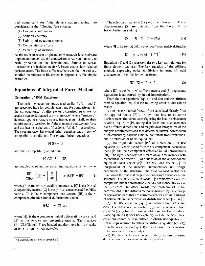
The solution of equation (1) yields the n forces [F]. The m
displacements fX_t J are obtained from the forces IFI by
backsubstitution (ref. 1):
IX] = [J] _[G] [F_ + [fl}0] (2a)
where [J] is the (m ×n) deformation coefficient matrix defined as
[J] = m rows of [[S]-Ilr (2b)
Equations (1) and (2) represent the two key IFM relations for
finite element analysis. The key equation of the stiffness
method, expressing nodal equilibrium in terms of nodal
displacement, has the following form:
[K] IX] = IP] + iPI' (3)
Equations of Integrated Force Method
Generation of IFM Equations
The basic WM equations introduced earlier (refs. 1 and 2)
are presented here for completeness and for comparison with
the SM equations.* A discrete or discretized structure for
analysis can be designated as structure (n,m) where "structure"
denotes type of structure (truss, frame, plate, shell, or their
combination discretized by finite elements) and n,m are force
and displacement degrees of freedoms (fof, do/"), respectively.
The structure (n,m) has m equilibrium equations and r = (n-m)
compatibility conditions. The m equilibrium equations
[BI [F] = _P_f_
and the r compatibility conditions
[CI[G] _F] = _6R]
are coupled to obtain the governing equations of the WM as
[CI[GI _-_ or [SI[FI = [PI ° (1)
where [B] is the (mx n) equilibrium matrix, [C] is the (r x n)
compatibility matrix, [G] is the (n × n) concatenated flexibility
matrix, [P] is the m-component load vector, [6R_ is the r-
component effective initial deformation vector,
[tSR_ = - [C] _31o
where I3]0 is the n-component initial deformation vector, and
[S] is the (n × n)WM governing matrix. The matrices
[B] , [C] , [G], and [S] are handed and they have full-row ranks
of m, r, n, and n, respectively.
*All symbols are defined in appendix B.
where [K] is the (m x m) stiffness matrix and [P]' represents
equivalent loads caused by initial imperfections.
From the IFM equations (eqs. (1) and (2)) and the stiffness
method equation (eq. (3)) the following observations can bemade:
(1) In |FM the internal forces tF_¢_are Calculated directly from
the applied loads IPl'. In SM one has to caiculate
displacements first from loads (by using the load-displacementrelation [K] __X_ -- IP], noting that loads and displacements
have different dimensions and magnitudes) irrespective of the
analysis requirements and then determine internal forces fromdisplacements by backsubstitution, coordinate transformations,
and differentiation or its equivalent.
(2) The right-side vector [P]" of dimension n in !FM
equation (1) is constructed from the m-component mechanical
loads [P] and the r-component effective initial deformations
I3RI. The right-side vector of dimension m in SM includes both
mechanical load vector t_P_Jof dimension m and m-componentequivalent load vector IP] i. The IFM load vector IP]" is
independent of the material characteristics and design
parameters of the structure. The total SM load vector is a
function of the material properties and design variables of thestructure. The SM equivalent loads ;D_ are nonzero even for
compatible initial deformations that do not induce stresses in
the structure. In other words the problem of initial
deformations in the stiffness method is handled by the conceptof equivalent loads that are n0nzei-o even for a frivial s[tuati0n
of compatible initial deformation distribution when [6R] = I0].
(3) The IFM equation (eq. (1)) contains both EE'S and
cc's. The stiffness equation (eql (3)) can be obtained from
equation (1) by transforming variables and backsubstituting.
Since equation (3) does not explicitly include the cc's, these
equations cannot be manipulated to Obtain 1FM equations.
The steps required to obtain the stiffness equation (eq. (3))
from the IFM equation (eq. (1)) are as follows (the derivation
is for mechanical loads only):
(l) Displacements are changed to deformations by using
deformation displacement relations (DDR'S):

[/31 = [B] fiX ] (4)
(2) Deformations are then transformed to forces by usingthe deformation force relation
{/31= [GIIFJ (5)
(3) Force displacement relafonsare obtained fromequafions(4) and (5) as
IF] = [G]-_03]rlXl (6)
(4) The upper portion of the EE of the _FMgoverning equation
(eq. (1), [B] IF} = [P]) is rewritten in displacements to obtain
the stiffness equation
[1131[G]- _[B]r] IX] = IPI (7)
or [K] IXI = [P], where [K] = [B] [G] - _[B] 7-. As mentioned
earlier the integrated force method cannot be obtained from
the stiffness formulation owing to the explicit absence of cc'sin that formulation.
1FM Solution Procedure
The IVMsolution procedure is illustrated in appendix A for
the example of a bar subjected to both mechanical and thermal
loads. The prinicipal steps are as follows:
Step 1: Assembly of the system equilibrium matrix [B].
The system EE matrix 03] is assembled from elemental
equilibrium matrices by standard finite dement techniques.The procedure to generate the elemental equilibrium matrix
is presented in the section "Equilibrium Equations" of this
report.
Step 2: Generation of the global compatibility matrix [C].
The generation of the global compatibility matrix is
presented in the section "Compatibility Conditions." Sincethe deformation displacement relation (eq. (4)) utilizes the EE
matrix 03] and the cc's are obtained from the DDR'S, accuracies
or errors in the equilibrium matrix are likely to be reflectedin the compatibility matrix [C].
Step 3: Generation of the concatenated flexibility matrix [G].
The block diagonal flexibility matrix [G] is obtained as the
diagonal concatenation of elemental flexibility matrices. The
elemental flexibility matrices are obtained by discretizing
complementary strain energy functionals according to standardflexibility techniques.
Step 4: Construction of load vector Ipl ".
The IFM load vector/P]' is assembled from mechanical loads
IPI and initial deformations I_/10 as defined in equation (1).
Step 5: Solution of IFM equation.
The matrix equation (1) is constructed from matrices [13], [CI,
and [G] and load [PI ", and its solution yields the forces. Dis-
placements are obtained by backsubstituting from equations (2).
Equilibrium Equations
The equilibrium equations, written in term of forces at the
grid points of a finite element model, represent the vectorial
summation of n internal forces IFI and m external loads [PI.The nodal EE in matrix notation gives rise to the (m × n)
(n >m)-banded rectangular equilibrium matrix ['B], which is
independent of the material properties and design parameters
of the indeterminate structure (n,m). For finite element analysis
this matrix is assembled from elemental equilibrium matrices.
The elemental equilibrium matrices 03] for bar and beamelements can be obtained from the direct force balance
principle (ref. 4). For continuous structures, such as plates
or shells, very few equilibrium matrices are reported in the
literature (refs. 17 and 18). Equilibrium matrices for the plate
flexure problem are given by Przemieniecki (ref. 17) and
Robinson (ref. 18). Przemieniecki generates the matrix for a
rectangular element in flexure from direct application of theforce balance principle at the nodes. Robinson utilizes the
concept of virtual work to derive the matrix for a rectangular-plate element in flexure. The procedures of Przemieniecki and
Robinson are documented in their books (refs. 17 and 18) andare not repeated here.
Energy-equivalent equilibrium matrices for finite dement
analysis can be obtained from the tVM variational functional
(ref. 7). The procedure to be followed to generate an elemental
equilibrium matrix from the IFM variational functional is
illustrated next for the example of a rectangular-plate element
in flexure. The portion of the IFM functional (ref. 7) that yields
the equilibrium matrix 03] for a plate bending element has the
following well-known form:
ffM. w MUp = _D( xOx2 "[- My_y2 + _YOxOYJdx dy (8)
where Mx, My, and Mxy are the plate bending moments and
02W 02W 02W
_X 2 ' 3y 2' OxOy
represent the curvatures. The plate domain is D and the
coordinates are (x,y).
By appropriate choice of force and displacement functions
the energy scalar Up can be discretized to obtain the elementalequilibrium matrix 03].
Up = IX] r[BI[F/ (9)

wheretheelementaldisplacementdegreesof freedom are
symbolized by Ixl and the elemental force degrees of freedom
by IF].
The force fields have to satisfy two mandatory requirements:
(1) The force fields must satisfy the homogeneous equilibriumequations (here the plate bending equations in the domain).
(2) The force components Fk (k = 1,2 ..... 9) must be
independent of one another. This condition ensures the
kinematic stability of the element. For the rectangular platethe force field is chosen in terms of nine independent forces:
as
(F) =<F1, F2..... F9)
Mx = Ft + F2x + F3y + F4xy
My = F 5 + F6x + FTy + Fsxy
M_=F9t (10)
The variation of the normal moments in the field is linear,
but the twisting moment is constant. The assumed moments
satisfy the mandatory requirements.
The displacement field that should satisfy the continuitycondition (ref. 19) is chosen in terms of 12 variables to match
the three dof (transverse nodal displacement w i and two
rotations Oxiand Oyi per node i for the four nodes) and can bewritten in terms of Hermite polynomials as
w(x,y) = HOl (x)Hol (y)X l + Hot (x)Hll (y)X2
+ Htl(X)Hol(y)X3 + HoI(X)Ho2(y)X4
+ H01 (x)H12(y)Xs + Hi1 (x)H_(y)X6
+ Ho2(x)Ho2(y)X7 + Ho2(x)Ht2(y)Xs
+ H12 (x)Hoz (y)X9 + H02 (x)Hot (y)Xto
+ Ho2(x)Hll(y)Xll + H12(x)Ho1(y)X12
(lla)
In equation (1 la) the Hermite polynomials are defined as
Hol(X) =x 3 _ 3a2x + 2a 3
4a 3
x 3 _ 3a2x - 2a 3Ho2(X) = -
4a 3
X 3_aX 2 _a2x+ a 3HH (x) =
4a 2
x 3 + ax 2 _ a2x - a 3H1", (X) --
- 4a 2
(l lb)
where X 1, X2 ..... X12 are the 12 dof and a and b are the
dimensions of the plate along the x and y directions,
respectively. The Hermite polynomials for the y coordinate
direction can be obtained by changing x and a to y and b,
respectively, in equation (1 lb). The displacement field (eq.(1 la)) gives rise to linear force distribution (eq. (10)) for the
plate bending problem.
The equilibrium matrix is obtained by substituting moments
from equations (10) and displacements from equations (11)
into the energy scalar given by equation (8) and integration.
The equilibrium matrix thus obtained is presented in table I.
The generation of the equilibrium matrix [B] from the IVM
functional is a general procedure applicable to any other typeof element. The matrix obtained from the functional is
henceforth referred to as the consistent equilibrium matrix[B]_.
The two equilibrium matrices of Przemieniecki and
Robinson, depicted in tables II and III, are compared with the
IFM consistent matrix for response accuracy. In this study the
analysis was carried out by WM following the five steps givenin the section "IFM Solution Procedure."
TABLE I.--IFM CONSISTENT EQUILIBRIUM MATRIX [B]s FORRECTANGULAR-PLATE ENDING ELEMENT
0 b 0 - 2b-" 0 0 a - 2a2 - 25 5
0 b2 0 - b3 2a---_2 ab - 2a2b 03 15 -a 5 5
b - ab - 2b2 2ab2 - a2 a35 5 0 0 3 15 0
0 b 0 2b2 0 0 - a 2a---_'_5 5
0 - b2 0 - b3 - 2a2 -- 2aZba ab3 15 5 5
- b - ab 2b2 - 2ab2 0 0 a_22 - a35 5 3 15 0
0 -b
b z0 --
3
-b -ab
0 -b
0 -b23
b -ab
0 -2b2 0 0 -a -2a2 -25 5
0 b3 2a2 2a2b 01"5 a _- ab 5
-2b2 -2ab2 0 0 -a2 --a3 05 5 3 15
0 2b----_2 0 0 a 2a_ 25 5
0 b3 - 2a2 2a2b-- -a ab -- 015 5 5
2b-"_'2 2ab2 0 0 a--_2 a-.-_3 05 5 3 15
=
6

TABLEII.--PREZEMIENIECKI'SEQUILIBRIUM MATRIX TABLE III.--ROBINSON'S EQUILIBRIUM MATRIX _]R FOR
[B]p FOR RECTANGULAR-PLATE BENDING ELEMENT RETANGULAR-PLATE BENDING ELEMENT
[Dimension of element, (a,b).]
0 2 0 0 0 0 0 -__22 -1b a
1 1 0 0 0 0 0 0 0
0 0 0 0 0 0 -1 1 0
-2 20 -- 0 - 0 0 0 0 1
b a
-l 1 0 0 0 0 0 0 0
0 0 -I -1 0 0 0 0 0
0 0 0 -_.22 0 2 0 0 -1a b
0 0 0 0 -1 -1 0 0 0
0 0 l -1 0 0 0 0 0
o o o o o -___22 o 2 ib a
0 0 0 0 1 -I 0 0 0
0 0 0 0 0 0 1 1 0
IFM Consistent Matrix Versus Przemieniecki's Matrix
The elemental discretizations by the IVMand Przemieniecki
approaches are identical in force and displacement degrees offreedoms, with fof = 9 and dof = 12 for both. This gives rise
to identical dimensions of 12 × 9 for both matrices [B] s and
[B]p. In the IFM approach the moment variables are in units
of moment per unit length (such as kip-inch per inch or
kilogram-meter per meter). Przemieniecki concentrates the
moments at the nodes, and this accounts for the dimension
change between the elemental matrices [B]_ and [B]e. Thenumber of nonzero entries in the Przemieniecki matrix is 28.
In contrast, there are 68 entries in the IFM matrix [B]_. The
Przemieniecki matrix can be viewed as a lumped version,
whereas the IFM matrix is consistent. The quality of the
response was ascertained by using both the matrices IBis and
[B]p to solve a finite element model of a clamped square plate
in flexure (plate material, steel; size, 40 in. (I01.6 cm); andthickness, 0.2 in. (5.08 ram)) with a concentrated load at its
center (P = 1000 lb (453.59 kg)). Other analysis features in
[Dimension of element, (a,b).]
0 - b 0 2__ 0 0 - a 2b2 25 5
0 3 0 i-5 a -ab 0
0 0 a23 15 0
0 b 0 -2b2 0 0 -a -2a2 -25 5
0 ----- 0 -- a -ab 03 15
b ab 0 0 3 15 0
o b o 2b2 0 0 a 2a__2 25 5
0 -b2 0 -a -ab 03 15
o 0 3 15 0
-2a20 -b 0 _ 0 0 a -25 5
1"-5 -a -ab 0
-b ab ["--_ _'_--] 0 0 -aZ a,._33 15 0L_Z_A _L_2__]
aBoxedelementshad coefficienl ch,_ged from I/3 in Robinson's maa'ixm 2/5 in IFMconsistentmatrix.
the IFM procedure, such as the flexibility matrix and
compatibility generation scheme, were kept identical for both
cases. The deflection at the plate center was chosen as the
parameter for comparison. This parameter was obtained in IFM
by first calculating forces from equation (1) and then
substituting IFI in equation (2). The displacement for this
problem as given by Timoshenko (ref. 20) had the following
value for the plate depicted in figure 1:
wc = 0.4072 in. (10.343 mm) (12)
The central displacements obtained with the two matrices
([B]_ and [B]p) for the two finite element models are
presented in table IV. Table IV shows that the central
deflection obtained with the Ir_i matrix [B]s converged toTimoshenko's series solution for the first model with four
elements. Przemieniecki's equilibrium matrix [13]e not only
yielded a higher value for the central displacement wc for the

/ /14 _ ?/
Figure 1 .--Clamped plate. Along clamped edges w = Ow/Ox = Ow/Oy = O.
TABLE W.--IFM ANALYSIS RESULTS--RESPONSE BY
PREZEM!ENIECKI MATRIX [B]p VERSUS IFM
CONSISTENT MATRIX [B]s
lTimoshenko's solution, w c = 0.4072 in. (10.343 mm).]
Number of
elements
4
16
Przemieniecki matrix
Central Error,
displacement, percent
in. mm
0.5054 12.8372 24.11
.5509 13.9929 35.29
IFM matrix
Central
displacement,
W c
in. mm
0.4083 10.3708
.4069 10.3353
Error,
percent
0.20
.07
four-element model, but also did not show the tendency of
monotonic convergence for the refined model consisting of16 elements.
IFM Consistent Matrix Versus Robinson's Matrix
The IFM matrix bears a remarkable resemblance to
Robinson's matrix except for the following;
(1) There is a change in sign between the two matrices, The
reason is that the IFM sign convention is opposite to that ofRobinson's notations.
(2) Some of the elements with coefficient 1/3 in Robinson's
matrix [B]R were changed to 2/5 in the IFM consistent matrix.This difference occurred for the 16 elements noted in table lII.
For the test example of a clamped plate, however, the
discrepancy had a negligible effect on the solution for moments
and displacements as shown in table V...... = 7 •
When element geometry becomes complicated, it is rather
difficult to generate the equilibrium matrix by vectorial
summation of forces (ref. 17) or by repeated use of virtual
influence coefficients fief. 18). Therefore it is recommended
that the elemental equilibrium matrices should be generated
by following the In consistent approach (ref. 7).
The equilibrium matrix [B]_ corresponds to three displace-
ment variables per node (displacement w and two rotations
0_ and Oy), giving rise to 12 variables per node. This ideal-ization requires a displacement polynomial with 12 unknowns.
Only 12-term Hermite polynomials are used to satisfy this
requirement. The 12-term Hermite polynomial is known to
cause convergency difficulties in the stiffness method. The
effect of the 12-term Hermite polynomial on solution accuracy
in the integrated force method was examined by using adisplacement function given by equation (13) to obtain another
equilibrium matrix, designated as [13]a. This displacement
function has the following form:
w(x,y) = oq + ot2x + o_3y + or4x2 + o_sxy + ot6y 2
+ OLTX3 + Otsx2y + otgxy 2 + o/loY 3
+ _llX3y + Otl_'y 3 (13)
The constants of the polynomial were related to nodal dof by
following standard finite element techniques, and the 12 x 9
equilibrium matrix [B] a was obtained from equations (8),
(10), and (13). Few coefficients of the matrices [B]_ and [B]aare different.
In order to examine the effect on the solution accuracy, the
clamped plate was analysed by using both equilibrium matrices[B], and [B]a along with the appropriate flexibility and
compatibility matrices as described in the subsection "IFM
Solution Procedure." The plate properties are defined in the
main section "Solution Accuracy." The central displacements
obtained for three idealizations (model 1 has 4 elements,
model 2 has 16, and model 3 has 36) by using the two matriceswere as follows:
(1) For EE matrix [B] s. The central displacements wc forthe three idealizations were 0.2041, 0.2035, and 0.2035 in.
(5.181, 5.169, and 5.169 mm), respectively.
TABLE V.--IFM ANALYSIS RESULTS--RESPONSE BY ROBINSON'S MATRIX [B]R VERSUS
RESPONSE BY IFM CONSISTENT MATRIX lB]s
Number of' Robinson's matrix IFM matrix
elements
4
16
Central
displacement,
wc
in. mm
0.4083 10.3708
.4069 10.3353
Moment at plate
center,
M_=uy
(kip in.)lin. (kg m)/m
0.193 87.544
.241 109.317
Central
displacement,
W c
in. mm
0.4083 10.3708
.4069 10.3353
Moment at plate
center,
(kip in.)lin. (kg m/m)
-0.193 -87,544
-.241 -109.317

(2) For EE matrix [B]a. The central displacements wc forthe three idealizations were 0.2041, 0.2035, and 0.2035 in.
(5.181, 5.169 and 5.169 mm), respectively.
For the problem both matrices gave identical values for the
central displacement. Moments obtained for both cases werealso identical.
In the stiffness method it is a known fact that the solution
is sensitive to the choice of displacement fields (refer to eqs.
(1 l) and (13)). In the IFM displacement fields do not have a
significant effect on solution accuracy. For the plate problem
the two different displacement fields given by equations (1 l)and (13) yielded identical results. This feature of WM is furtherelaborated in the subsection "Element Level Effect."
Compatibility Conditions
The compatibility conditions are constraints on strains, and
for finite element models they are also constraints on member
deformations [/31. The n-component deformation vector isdefined as
I/3} = [G] [F t + I/3}o (14)
where I/3] is the total deformation, [G] is the flexibility matrix,
IF1 represents the member forces, and [/31o is the initial
deformation. When expressed in terms of force variables the
cc's involve two matrices, the flexibility matrix [G] and the
compatibility matrix [C], and can be written as
[C][G] [F] = {6R] (15)
This equation augments the EE'S in the IFM as given in
equation (I). The flexibility matrix [G] is obtained from the
discretization of the complementary strain energy by following
standard techniques. For the plate element example the
flexibility matrix [G]e can be symbolically represented as
1
U c = _ [F] T[Gle{F ]
(16)
where D 1 = (Eh3/12), E is Young's modulus, u is Poisson's
ratio, and h is the plate thickness.
Substituting into equation (16) the moments Mx, My, and
Mxy in terms of forces F1, F 2 ..... F9 as given by equation(10) and integrating yield the (9 x 9) flexibility matrix [G]e
for the rectangular-plate flexure element. The generation ofthe flexibility matrix [G] is reported in the literature (refs. 4,
17, and 18) and will not be repeated here. The system
flexibility matrix [G] for the structure is a block diagonal
matrix. It is obtained as the diagonal concatenation of element
flexibility matrices.
Generation of Compatibility Matrix [C]
The compatibility matrix [C] is obtained by extending
St. Venant's theory of elasticity strain formulation to discrete
structural mechanics (refs. 11 and 12). The procedure is
illustrated by taking the plane stress elasticity problem as an
example. The strain displacement relations (SDR'S) of the
problem are
Ouf-x _ -- |
Ox
t
Ov
ey Oy
Ou Ov
"Yxy= yO--+ Ox
(17a)
In the SDR'S three strains (ex, %., and 3%) are expressed asfunctions of two displacements (u and v). The compatibility
constraint on strains is obtained by eliminating the two
displacements from the three SDR'S, resulting in the single
compatibility condition
°32e_x + 02e2 -- 32TaY = 0
Oy2 Ox2 OxOy(17b)
The two steps of St. Venant's procedure to generate cc's areas follows:
(1) Establish the SDR'S.
(2) Eliminate displacements from the SOR'S to obtainthe cc's.
The equivalents of SDR'S in the mechanics of discrete structures
are the deformation displacement relations (DDR'S);
deformations I/3] of the discrete analysis are analogous to
strains [e] of the elasticity analysis. The DDR'S can be assembled
directly or obtained on an energy basis.
The well-known equality relating internal strain energy and
external work can be written for a discrete structure (n,m) in
the following form:
[F} r[/3} = 2 [X] r[p] (18a)
where IX] are the nodal displacements. Equation (18a) can
be rewritten by eliminating loads IPI in favor of forces IF]
and using the EE (Ill IF] = [PI) to obtain the following
relationship:

1 1IX]r[B][FI = _ IFl rl/3t (18b)
or
_1[FIr([B] r[Xl _ [/3]) = 0 (18c)2
Since the force vector IF] is not a null set, we finally obtain
the following relation between member deformations and nodal
displacements:
[/31 = [B] r IX] (19)
The expression given by equation (19) is the general DDRapplicable to finite element models whose EE'S can be
symbolized as [B] IF1 = [PI- In the DDR n deformations are
expressed in m displacements; thus there are r = (n-m)
constraints on deformations that represent the cc's of the
structure (n,m). The cc's are used to augment the EE'S,
completing them to an n x n set. The r = (n -m) co's, which
are obtained by eliminating m displacements from n DDR, can
be symbolized in matrix notation as
[C] [/3] = [01 (20)
In equation (20), [C] is the (r x n) compatibility matrix. Itis a kinematic relationship and as such it is independent of
design parameters, material properties, and external loads. The
matrix is rectangular and banded. The maximum bandwidth of
cc matrix [C] of an element in a finite element model depends
on the force degrees of freedom (for) of its neighboring
elements. The maximum bandwidths of the compatibility
conditions for the plate in flexure with fof = 9 shown infigure 2 are as follows: the maximum bandwidths (MAW) of
compatibility conditions for the plate can be obtained as afunction of the element location in the finite element model as
Interior element Maw = 81 Zone 1
Boundary element Maw = 54 Zone 2Corner element Maw = 36 Zone 3
Th e generation.of banded comPat!bility., cond!tions - isamenable to computer automation (refs. 11 and 12). The
compatibility conditions of finite element analysis are
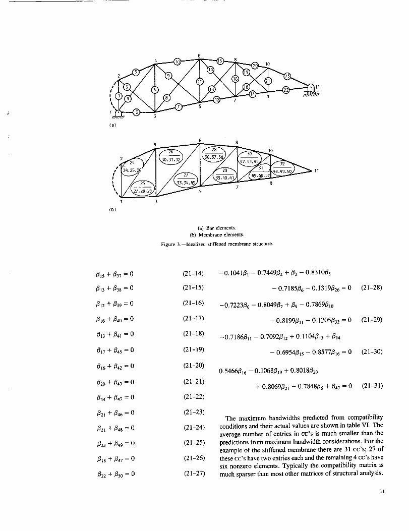
illustrated by taking the example of a stiffened membrane(fig. 3). The finite element model of the structure consists of
9 triangular membrane elements and 23 bars. Each membraneelement has three fof; the bar has one fof. The total number
of force variables is n = 50, consisting of 9 × 3 = 27membrane forces and 23 bar forces. The structure has 11
nodes, each free node has two dof. Node 1 is fully restrained;node 11 is partially restrained. The number of displacement
degrees of freedom m=(lI ×2-2-1)= 19. It hasr = (n-m) = 31 compatibility conditions. The cc's in terms
CBW - BANDWIDTH OF COMPATIBILITY CONDITIONS
EBW - BANDWIDTH OF EQUILIBRIUM EQUATIONS
FEM FINITE ELEMENT DISPLACEMENT METHOD (12 DEGREES OF FREEDOM)
IFM = INTEGRATED FORCE METHOD <NINE DEGREES OF FREEDOM)
PI rt
: I
ZONE 3
i
r
_ --%- iZONE I i
CBW = 9x9 = 81
EBW = 4x12 = t18 :
o , o o
o p
iI
i
CBW _ qx9 = 36EBW hx12 = 48
11.....
[r
0
: 2
o
• CBW = 6x9 = 54 (IFM)
EBW = qx12 = h8 (FEM)
EBW 4x9 _ 36 (IFM)
F
I
L
=
Figure 2.--Bandwidth of compatibility conditions and equilibrium equations
for clamped plate.
of member deformations as obtained from St. Venant's strain
formulation for finite element analysis of the stiffenedmembrane are as follows:
/34 + /326 = 0 (21 - 1)
/31 + _24 = 0 (21-2)
/_5 + /325 = 0 (21-3)
/32 + /327 = 0 (21-4)
/36 +/328 = 0 (21-5)
-- /326 + /329 = 0 (21-6)
/36 +/330 = 0 (21-7) ==
/310 +/331 = 0 (21-8)
/38 -'1- _32 = 0 (21-9)
/37 + /_33 = 0 (21-10)
P]I +/334 = 0 (21-II)
-- /_32 -'l- /335 = 0 (21-12) _
/311 + t336 = 0 (21-13)
l0
6
(a)
6
11
7 $
(b)
(a) Bar elements.
(b) Membrane elemems.
Figure 3.--Idealized stiffened membrane structure.
/315 ''[" /337 = 0 (21-14)
/313 + /33S = 0 (21-15)
812 + 839 = 0 (21-16)
/3t6 + /34O= 0 (21-17)
/313 -k-/341 = 0 (21-18)
1317+ 1345= 0 (21-19)
816 + 842 _---0 (21-20)
/32o+/343 = 0 (21-21)
844 + /347= 0 (21-22)
/_Zl + 1346= 0 (21-23)
/32l -Jr-/348 "_"0 (21--24)
/323 + 849 = 0 (2 1--25)
818 q"/347 = 0 (21--26)
/322 + 850 = 0 (21-27)
-0.1041/31 - 0.7449/32 +/33 - 0.831085
-- 0.7185/36 - 0.1319/326 = 0
-0.7223/36 - 0.8049/37 + 89 - 0.7869/310
- 0.8199/311 - 0.1205/332 = 0
-0.7186811 - 0.7092/312 + 0,1104/313 +/314
- 0.6954/315 - 0.8577/316 = 0
0.5466/316 -- O. 1068/319 + 0.8018820
+ 0.8069/321 - 0.7848/36 +/347 = 0
(21-28)
(21-29)
(21-30)
(21-31)
The maximum bandwidths predicted from compatibilityconditions and their actual values are shown in table VI. The
average number of entries in cc's is much smaller than the
predictions from maximum bandwidth considerations. For the
example of the stiffened membrane there are 31 cc's, 27 of
these cc's have two entries each and the remaining 4 c¢'s have
six nonzero elements. Typically the compatibility matrix ismuch sparser than most other matrices of structural analysis.
I1

TABLE VI.--BANDWIDTH OF COMPATIBILITY CONDITIONS
Prediction from bandwidth Actuals
consideration
Maximum Minimum Maximum Average MinimumT
52 [ 18 6 a3 23-
aRounded to next higher number,
Physical Interpretation of Compatibility Conditions
A finite element model has numerous interelement
boundaries. From the viewpoint of continuum analysis the
boundary compatibility conditions along these interelement
boundaries also have to be satisfied. The conditions along the
element interface can be symbolized as
_RI + 6RII = 0 (22a)
where (6m,6m0 represent the residue in the Bcc's of the two
neighboring elements I and II, respectively. For the membrane
problem the residue 6R can be represented in the followingform (ref. 7):
0 (Ny -- vNx)n x + (N x - vNy)nyTx
- (1 + _,) (Nxy)ny+ _ (N.)nx (22b)
where Nx, Ny, and N_ are the membrane stress resultants and
nx and lqy represent the direction cosines of the outwardnormal for the element interface.
The equality constraint given by equation (22a) ensures
interelement boundary compatibility. The correct stress fieldsshould satisfy the interelement BCC'S given by equation (22a).
Element interphase boundaries could be of complicated
geometry; in consequence it is rather difficult to explicitly
satisfy the interelement BBC'S given by equation (22a) apriori
by choosing appropriate displacement or stress fields, or both.
The satisfaction of interelement strain compatibility, and not
just displacement continuity, is a neglected condition in the
popular stiffness method formulation. In general, stresses
obtained by displacement formulation along the element
interface boundary satisfy neither equilibrium nor compatibilityconditions. (Because of this limitation in the stiffness-based
finite element method, stress computation is typically avoided
at the cardinal node points or along element interphases.)
In the integrated force method interelement BBC'S areautomatically enforced via the cc's
f[C] Ifll = [C] [G] IF_ = t_R_
The cc's between elements at interfaces are satisfied by theconstraints given by equations (21-I) to (21-27). Take
equation (21-12) for example. This constraint enforces
interelement deformation continuity or BCC'S between
membrane elements 26 and 27 along the interelement boundarydefined by nodes 3 to 6 as depicted in figure 4(a). Such
interelement cc's are designated by the symbol (MM),
membrane-to-membrane compatibility, in figure 4(a). Take
the next cc given by equation (21-13). This constraint enforcesdeformation balance conditions between membrane 27 and
bar 11 along the interface defined by nodes 5 and 6. These
types of cc's are symbolized by BM, bar-to-membrane
compatibility, in figure 4(a). The total number of interphase
cc's (both MM and BM) is 27 as shown in figure 4(a). Besides
these cc's there are four bay cc's; these enforce deformation
balance conditions of six adjoining bars as shown infigure 4Co).
In the integrated force method the equilibrium conditions
are satisfied at the nodes [B] iFi = iP], the same as attempted
by the stiffness method. In addition, the following cc's aresatisfied only in the IFM:
(I) Membrane-to-membrane compatibility
(2) Membrane-to-bar compatibility
(3) Compatibility between a group of bars
For this example the EE'S number 19 and the cc's number 31.
The IFM satisfies all 50 equations. In contrast, the stiffnessmethod is based on the 19 EE'S expressed in displacements;
the 31 cc's are more or less ignored. Since it is mandatoryfor the stress fields to satisfy the cc's, their exclusion in the
stiffness method reflects on the accuracy of the stress fields.
Computer Automation of Formulations
Modern structures, because of their complexity, have to be
analyzed by digital computers. Computer automation is
therefore an essential requirement of analysis formulation
despite its other merits and limitations. The integrated force
method satisfies this requirement, since all three matrices
(equilibrium matrix [B], compatibility matrix [C], and
flexibility matrix [G]) are amenable to automatic generation
on a digital computer. Since the stiffness method is known
to be amenable to computer automation, both the IFM and the
SM satisfy this requirement.
Solution Accuracy
E
The accuracy of solutions obtained either by IFM or SM is
of paramount importance in the choice of analysis formulation.
During the formative period of finite element analysis Argyris
(refs. 21 and 22) solved several problems both by theclassical
force method (SFM) and the stiffness method. Scrutiny of thisTake the example of the stiffened membrane shown in figure 3.
m
12

INTERFACE COMPATIBILITIES
(_ MEMBRANE TO MEMBRANE
(_ BAR TO MEMBRANE
6
I 3
(a)
6 6
9
I 3 3
(b)
(a) Interface.
(b) Bay.
Figure 4.--Compatibilities of stiffened membrane structure.
study indicates that the SFM predicted more accurate stress
solutions for almost all examples, including plates and
cylinders, whereas inaccuracies can be noticed in the stiffnesscomputations. The Irr,_ retains all the favorable features of the
classical force method (s_) as far as solution accuracy is
concerned. Consequently Jr'M predictions have to be as accurateas Argyris's SFM results.
To check the accuracy of solutions between the integratedforce method and the stiffness method in the context of finite
element analysis, we developed two plate bending elementsfor the IFM:
(1) A rectangular element with four nodes
(2) A triangular element with three nodes
The quality of solutions obtained by the Ir-_ and the SM was
compared for both types of elements by taking the example
of clamped plate bending under a concentrated load. The plateparameters were as follows:
Size of plate, a = b, in. (cm) ...................... 40 (101.6)
Thickness of plate, h, in. (mm) .................... 0.2 (5.08)
Young's modulus, E, ksi (kg/mm 2) .... 30 000 (21 091.81)
Poisson's ratio, v ............................................... 0.3
Magnitude of concentrated load at
center, P, lb (kg) ............................... 500 (226.795)
In the stiffness method nodal stress parameters calculated by
backsubstituting from grid point displacements are discon-
tinuous and ambiguous (ref. 9). Calculating forces at the nodes
is routinely avoided in the stiffness method. Because of that
the noncontroversial nodal displacement was used in the
comparison. It should, however, be remembered that in the
IVMforces are the primary variables from which displacements
are obtained by backsubstitution.
The central deflection of the plate given by Timoshenko
(ref. 20) is
wc = 0.2036 in. (5.715 mm)
For the stiffness analysis two well-known analysis codes, ASKA
(ref. 23) and MSC/NASTRAN (ref. 24), were used. The types
of plate bending elements used were(1) QUAD-4: Rectangular element with 12 degrees of
freedom. Both ASICAand MSC/NASTRANhave QUAD--4 elements.
(2) TaIB-3: Triangular element of the ASKAprogram with
nine degrees of freedom.
(3) TUBA-3: Higher order triangular element of the ASKA
program with 18 degrees of freedom.
(4) TRIA-3: Triangular element of MSC/NASTRAN with nine
degrees of freedom.
13

The first three elements are well known in the literature and
are popular in practice. The QUAD--4, a quadrilateral element
with six dof per node was used here as a rectangular fiat-plate
element with three dof at grid points with appropriate
specialization. Likewise fiat-plate elements were obtained from
the triangular elements of the general-purpose program.
Analysis by ASKA Code
QUAD-4 is a rectangular element, it has three dof per node,
consisting of transverse displacement w and two rotations (0x
and 0), and its in-plane rotation is restrained. The element
displacement field corresponds to a cubic displacementfunction with 12 constants. TRIB-3 and TUBA-3 of the ASKA
code are triangular elements. TUBA-3 is a higher order element
with 18 degrees of freedom. It has six degrees of freedom per
node consisting of one displacement, two slopes, and three
curvatures. TRIB-3 is a plate element with 9 degrees of
freedom. It has three degrees of freedom per node consisting
of one displacement w and two rotations (0_ and Oy).The results obtained for the central displacement wc by
using ASKAQUAD-4, TRIB-3, and TUBA-3 elements are presentedin table VII for several finite element idealizations, shown in
figure 5. The central displacement obtained by using the ASKA
QUAD-4 element tended to converge to Timoshenko's solutionfor the finite element model with 64 and 100 elements at a
residual error of about 2 percent. As table VII shows, there was
no substantial difference in the convergence rate for the two
triangular elements. As before, the stiffness method required a
very fine mesh of about 128 elements to show some convergencyto the closed-form solution. For the 128-element model the
residual error was about 10 percent for TUBA-3 and 6 percentfor TmB-3.
MSC/NASTRAN Verification
The example of a clamped plate under a central concentrated
load as shown in figure 1 was again solved, this time by using
3t 13 14 15 16
9 10 11 12~.
5 6 7 8
1 I 2 3 4
4 ELEMENTS 16 ELEMENTS
(a)
q ELEMENTS
(b)
8 ELEMENTS 32 ELEMENTS
(a) Rectangular elements.
(b) Triangular elements.
Figure 5.--Discretization of plate by using rectangular and triangular finiteelements•
the QUAD-4 element of the NASA structural analysis codeMSC/NASTRAN. The QUAD-4 elements of the MSC/NASTRANand
ASKA codes are identical with respect to the two fundamental
element characteristics, such as the number of nodes and the gridpoint displacement degrees of freedom. Results obtained for three
models with 4, 16, and 36 elements, respectively, are presentedin table VIII.
As tables VII and VIII show, the agreement in the results
obtained by the two codes (MSC/NASTrAN and ASK-a) forthe
problem was good. For 4 and 16 elements the ASKA results
were marginally better than the MSC/NASTaAN solution.
However, MSC/NASTRANshowed monotonic convergence with
a residual error of 0.29 percent for the 36-element model,
Number of
elements
4
8
16
32
64
103
128
.... TABLE VII.--ASKA CODE ANALYSIS RESULTS
ITimoshenko's solution, w e = 0.2036 in. (5•715 mm).]
QUAD--4 rectangular element
Central Error,
displacement, percent
in. mm
0.0409 1.0388 80.03
.1995 5.0673 2.04
.2092 5.3137 2.75
.2092 5•3137
2•75
TRIB-3 triangular element
Central Error,
displacement, percent
wc
in. mm
0.0860 2.1844 57.76
.0650 1•6510 68.07
• 1547 3.9294 24.01
.1837 4.6660 9.82
TUBA-3 triangular element
Central Error,
displacement, percent
Wc
in. mm
0.0771 1.9583 62.13
.0641 1•628 68.51
.1607 4.0818 21.07
.1910 4.8514 6.18
t
14

TABLEVIII.--MSC/NASTRANANDIFM ANALYSIS RESULTS
[Timoshenko's solution, we = 0.2036 in. (5.1715 mm).]
Number of
elements
4
16
36
NASTRAN QUAD-4
Central Error,
displacement, percent
wc
in. mill
0.027 0.686 86.75
.1914 4.862 6.02
.2042 5.187 .29
IFM rectangular element
Central Error,
displacement, percent
i%
in. mm
0.2041 5.1842 0.20
.2035 5.1689 .05
.2035 5.1689 .05
whereas the ASKA code exhibited a residual error of about
2 percent for a 100-element model.
Analysis by Integrated Force Method
The WM rectangular element assumes cubic distribution for
displacements (eq. (11) or (13)) and linear distribution for forces
(eq. (I0)). This element corresponds to the QUAD-4 element,
which also has three displacement degrees of freedom per node,
consisting of displacement w and two slopes (Ox and 0y) for itsfour nodes. As far as displacement and force degrees of freedom
and number of nodes are concerned, all three elements 0FM,
ASKA, and MSC/NASTRAN) are equivalent. The results obtained
by WM for three different finite element models are given in tableVII/. Remember that in IFM the forces are calculated first and
then the desired displacements are obtained from the forces by
backsubstitution. For the purpose of comparison, however, only
displacement is presented, since only this variable is directlycalculated in the stiffness method as mentioned before.
Table VIII shows that convergence occurred for the first
model, consisting of four elements. If symmetry is taken into
consideration, convergence will occur for a single element. The
residual error for the four-element model was 0.2 percent, and
it was reduced to 0.05 percent for the second model, which had
16 elements. Results obtained for the rectangular element by
using WM and the two well-known displacement-based finiteelement programs (ASKA and MSC/NASTRAN) are presented
graphically in figure 6. The rFM results are barely discernible
from Timoshenko's solution, whereas the ASKAand MSC/NASTRAN
results converge slowly.
MacNeal and Harder (ref. 25) introduced a grading scheme
for the evaluation of finite elements, as follows:
A = less than 2 percent error
B = 2 to 10 percent error
C = 10 to 20 percent error
D = 20 to 50 percent error
F = greater than 50 percent error
The comparative merits of WM, ASKA, and MSC/NASTRANresults on the basis of residual error are given in table IX,
which is based on MacNeal's grading scheme. The WM element
7:
1,25 --
1.00
.75 --
.50 --
.25 --
METHOD
TIMOSHENKO
_"0-_ INTEGRATED FORCE
---{]---- ASKA OUAD-4
-,---L_-_ MSC/NASTRAN QUAD-q
,,'/
,,;/
,,'/
i I t I till I ,
101
NUMBER OF ELEMENTS, LOG (N)
o I I , I,I,I100 102
Figure 6.--Convergence analysis of clarntxxl plate with concentrated load
by using rectangular or quadrilateral finite elements.
scored an "A" grade for the first model, consisting of four
elements only. MSC/NASTRANQUAD--4required 36 elements to
reach "A", and ASKAQUAD--4Was unable to achieve an "A"even with 100 elements.
Results for Triangular Elements
The convergency for the problem using triangular elements
of the IVM and stiffness codes (ASKA and MSC/NASTRAN) is
presented in figure 7. The grades secured by the elements are
given in table IX. The WM result was discernible from the
TABLE IX.--MacNEAL'S GRADE CARD
(a) Rectangular element "report card"
Number of IFM MSC/NASTRAN
elements rectangular QUAD-4
4
16
36
64
100
A
A
A
F
B
A
A
ASKA
QUAD-4
F
B
B
B
(b)Triangular element "relx)rt card"
Number of
elements
4 B
8 A
16
32 ---
128 ---
MSC/NASTRAN
TRIA-3
IFM
rectangular
F
D
C
B
ASKA
TRIB-3 TUBA-3
--- F
F F
C D
B B
15
tt_
a_
1.25 --
1.00
.75 --
•50 --
.25 --
0I00
_THOD
TIMOSHENKO
_..(:)-m INTEGRATEDFORCE---_--- ASKA_IB-3-_-_ ASKATUBA-3--"-<_---- MSC/NASTRANTRIA-3
m;
o--'_ o,/ .-_":""
/
g__J_____ I I IIii[ I I I I l_IIl
101 102
HUMBEROF ELE_NTS, LOG(N)
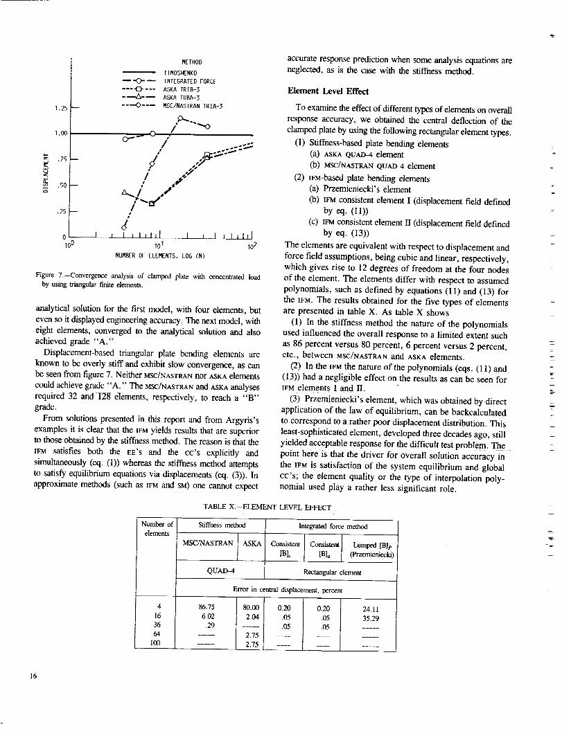
Figure 7•--Convergence analysis of clamped plate with concentrated load
by using triangular finite dements.
analytical solution for the first model, with four elements, but
even so it displayed engineering accuracy. The next model, with
eight elements, converged to the analytical solution and also
achieved grade "A."
Displacement-based triangular plate bending dements are
known to be overly stiff and exhibit slow convergence, as can
be seen from figure 7. Neither MSC/NASTRAN nor ASKA dements
could achieve grade "A." The MSC/NASTRAN and ASKA analyses
required 32 and128 elements, respectively, to reach a "B"
grade.
From solutions presented in this report and from Argyris's
examples it is clear that the IF_ yields results that are superior
to those obtained by the stiffness method. The reason is that the
IFM satisfies both the EE'S and the cc's explicitly and
simultaneously (eq. (1)) whereas the stiffness method attempts
to satisfy equilibrium equations via displacements (eq. (3)). In
approximate methods (such as IFr_ and SM) one cannot expect
accurate response prediction when some analysis equations are
neglected, as is the case with the stiffness method.
Element Level Effect
To examine the effect of different types of elements on overall
response accuracy, we obtained the central deflection of the
clamped plate by using the following rectangular element types.
(1) Stiffness-based plate bending elements
(a) ASKA QUArt-4 element
(b) MSC/NASTRAN QUAD-4 element
(2) r_-based plate bending elements
(a) Przemieniecki's element
(b) Ir'M consistent element I (displacement field defined
by eq. (1 I))
(c) rFM consistent element II (displacement field defined
by eq. (13))
The elements are equivalent with respect to displacement and
force field assumptions, being cubic and linear, respectively,
which gives rise to 12 degrees of freedom at the four nodes
of the element. The elements differ with respect to assumed
polynomials, such as defined by equations (11) and (13) for
the wr, l. The results obtained for the five types of elements
are presented in table X. As table X shows
(1) In the stiffness method the nature of the polynomials
used influenced the overall response to a limited extent such
as 86 percent versus 80 percent, 6 percent versus 2 percent,
etc., between MSC/NASTRAN and ASKA elements.
(2) In the IFM the nature of the polynomials (eqs. (11) and
(13)) had a negligible effect on the results as can be seen for
IFM elements I and II.
(3) Przemieniecki's element, which was obtained by direct
application of the law of equilibrium, can be backcalculated
to correspond to a rather poor displacement distribution. This
least-sophisticated element, developed three decades ago, still
yielded acceptable response for the difficult test problem. The
point here is that the driver for overall solution accuracy in
the n:u is satisfaction of the system equilibrium and global
cc's; the element quality or the type of interpolation poly-
nomial used play a rather less significant role•
TABLE X.--ELEMENT LEVEL EFFECT
Number of
elements
4
16
36
64
100
Stiffness method
MSC/NASTRAN ASKA
QUAD-4
Integrated force method
Consistent Consistent Lumped IB]e
IB]_ [13L CPrzemieniecki)
Rectangular .%menl
Error in central displacement, percent
86.75 80.00 0.20 0.20 24.11
6.02 2.04 .05 .05 35.29
.29 .05 .05
2.75
2.75
r
±
16

Conditioning of Equations ofIFM Versus SM
Finite element analysis requires the solution of a large
number of simultaneous equations. Hence the stability of the
equation is a primary criterion in the choice of analysis
formulation. The Ir_ matrix [S] is not symmetric, whereas
the sM stiffness matrix [K] is symmetric. The matrix [S] is
of higher dimension than the stiffness matrix [K]. The normsof the i_a upper equilibrium matrix [B] and lower cc matrix
[G] in equation (1) differ substantially. It may therefore be
suspected that the IFM equation that contains both EE'S and cc'sis an ill-conditioned system. In order to examine the issue,
we analyzed several problems (1) by scaling the cc's and (2)
without any scaling at all. Scaling had no effect on the solution:
the IV-Mlost only one or two precision points in 14-digit
arithmetic for almost all problems solved.
We further compared IFMand SM equations numerically for
a few different types of structures. The equation stability of
sra is governed by the parameter z, defined as
_rflax
z - (23a)_min
where _max and _kmi n are the maximum and minimum
eigenvalues, respectively, of the symmetric stiffness matrix
[K]. The equation stability of IFM matrix IS] is governed by
the parameter y defined as
Smax
y = -- (23b)Smin
where Sr_x and S_n are the maximum and minimum singular
values, respectively, of the nonsymmetric matrix [S]. Weevaluated z and y for several structure types and some results
are presented in table XI. For the examples solved, the
eigenspace of matrix [S] was much less distorted than that ofthe stiffness matrix [K]; that is,
£e=->> 1 or z>>y (24)
Y
Since z is greater than y, the imcl equations were more stable
than the sM equations. One need not be influenced by the
simple fact that the SM stiffness matrix [K], being symmetric,
should possess better conditioning than the wM matrix [S]. The
reason is that the symmetric stiffness matrix [K] is a productof three matrices, [K] = [B] [G]-I[B] r, and successive
matrix multiplications and inversions deteriorate its stability.
The im,_ matrix [S] is well conditioned. The integrated force
method thus gave rise to a superior set of equations than didthe stiffness method.
TABLE XI.--STABILITY OF EQUATIONS--STIFFNESS
METHOD VERSUS INTEGRATED FORCE METHOD
Type of Stiffness method, Integrated force method
structure z = _max/_kmin Y = Smax/Smin
Truss (6,4)
Truss (16,13)
Truss (26,21)
Truss (36,29)
Frame (9,6)
Frame (18,12)
Frame (27,18)
!Frame (36,24)
Plate (9,6)
Plate (18,12)
Plate (27,18)
Plate (36,24)
16.47
218.50
1 598.10
3 378.37
1 335.96
7 840.99
21 573.55
34 533.71
4 790.65
23 759.55
51 089.50
75 191.74
2.96
3.17
7.31
45.89
3.65
6.96
10.20
7.48
18.75
29.89
56.11
64.56
Sparsities of [B], [C], [S], and [K] Matrices
Comparison of Sparsities
Matrix sparsity and bandwidth are important parameters in
the finite element analysis. These parameters of the compati-
bility matrix [C] were compared with the same parameters of
the equilibrium matrix [B] for three types of structures
designated according to the notation introduced earlier as truss
(101,81), frame (99,66), and plate (99,66). The structures are
shown in figure 8. The properties of the associated symmetricstiffness matrix [K] were included for baseline reference. The
parameters of the matrices are tabulated in table XII. As can
be seen, the sparsities of the EE matrix IB] and the cc matrix
[C] were comparable but smaller than those of the stiffness
matrix [K]. The bandwidths of the matrices [B], [C], and [K]were more or less comparable. Within the bands the matrices
[13] and [C] were sparser than the stiffness matrix [K]. The
flexibility matrix [G] is a concatenated matrix, and its maxi-
mum bandwidth, which depends on the number of force vari-ables of the elements, was much smaller than dimension n of
matrix [S]. The internal sparsity of the flexibility matrix
enhanced the zero population of the system matrix. The
sparsities of the matrices [S], [C], and [B] for three otherstructures are shown in table XII.
From table XII and several other examples solved, it was
a common observation that the governing IFM matrix [S] was
much sparser than the equilibrium matrix [B] or the stiffness
matrix [K]. As already noted, the compatibility matrix [C]
appeared to be the sparsest among the structural analysismatrices ([B], [S], and [K]).
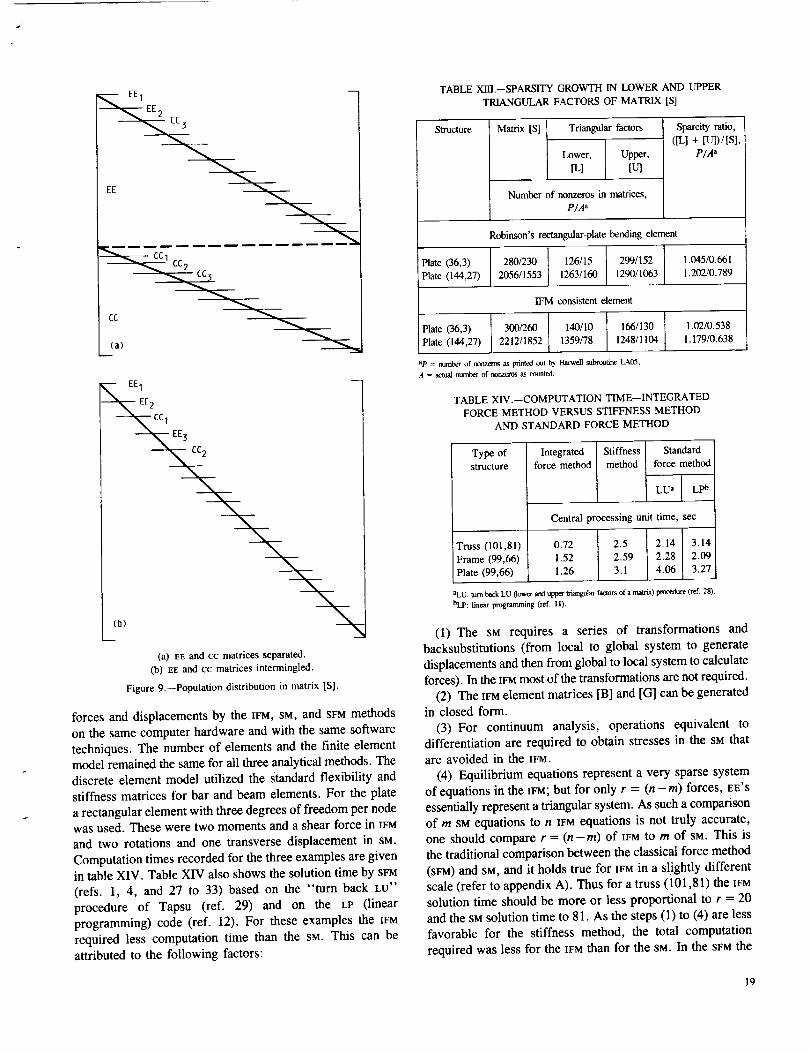
Sparsity Growth During Factorization of Matrix [S]
The WM equation system has population along two diagonals
as depicted in figure 9(a): EE population along the top diagonal
17

® ® ® // @(a)
®
(b)
(c)
(a) Twenty-bay truss.Co) Eleven-sto_ frame.
(c) Eleven-element cantilevered plate.
Figure 8.--Three structures used.
and cc population along the bottom diagonal. This
unconventional feature of the [S] matrix was avoided by
generating adequate numbers of EE'S followed by cc's based
on cc bandwidth information. The process was repeated and
a banded [S] matrix was obtained as depicted in figure 9(b).
Sparse matrix algebra along with a nonsymmetric matrix solver
(LA05 (ref. 26)) is used for IFM analyses. In order to avoid
the deterioration of sparsity during solution, the symmetric
stiffness matrix is typically factored ([K] = [L] [U]), where
the [L] and [U] are upper and lower triangular matrices. The
population inside the band for the symmetri c stiffness matrix[K] is equal to the sum of its factors ([L] + [U]). The question
is, What is the sparsity increase during the factoring of theIS] matrix? This issue (IS] = ILl[U]) was examined
numerically for a few examples, as given in table XIII. The
factoring was carried out by the Harwell library sparse solver
LA05. In the examples solved, the actual nonzero populationof the sum of the triangular matrices (ILl + [U]) was somewhat
less than the sparsity of the [S] matrix. The program LA05,
however, printed a minor growth in sparsity ratio. This
deviation was not a deficiency of the structure of the [S] matrix
but was attributed to the storage scheme used and to the degree
of compaction in the algorithm at the time of printing.
Comparison of Computation Time
The IFM matrix [S] is unsymmetrical and its dimension is
(n x n). The SM matrix [K] is symmetrical and its dimensionis (mx m), where n >_ m. From this information alone, foridentical idealization of a structure with the same number of
elements it can be argued that s0]ution by IFM should be
numerically more expensive than solution by SM. To examine
this issue, we solved three examples (a truss, a frame, and
a plate, each with approximately 100 degrees of freedom) for
TABLE XII.--SPARSITY OF MATRICES [B], [C], AND [K]
Type of
structure
Truss (101,81)
Frame (99,66)
Plate (99,66)
....!Bl lSparsity,percent
IK]
4.82 5.94 14.5
6.85 6.52 17.34
4.53 4.44 25.91
Matrix
Bandwidth
Average Maximum
8 6 10.91 8 6 12
11.45 12.45 10.91 12 14 12
17.18 8.82 17.10 18 16 18
=-_
Ig
'1[
Type of Sparsity ratio
structure
[s] IBI [c]
Truss (176,141) 0.022 0.020 0.034
Plate (144,27) .075 .126 .039
Plate (36,3) .144 .450 .036
18
EEl
EE2
cc
(a)
CC3
(a) EE and cc matrices separated.
(b) EE and cc matrices intermingled.
Figure 9.--Population distribution in matrix [S].
forces and displacements by the IFM, SM, and SFM methods
on the same computer hardware and with the same softwaretechniques. The number of elements and the finite element
model remained the same for all three analytical methods. The
discrete dement model utilized the standard flexibility and
stiffness matrices for bar and beam elements. For the plate
a rectangular element with three degrees of freedom per nodewas used. These were two moments and a shear force in ]FM
and two rotations and one transverse displacement in SM.
Computation times recorded for the three examples are givenin table XIV. Table XIV also shows the solution time by SFM
(refs. 1, 4, and 27 to 33) based on the "turn back LU"
procedure of Tapsu (ref. 29) and on the LP (linear
programming) code (ref. 12). For these examples the IFM
required less computation time than the SM. This can beattributed to the following factors:
TABLE XIII.--SPARSITY GROWTH IN LOWER AND UPPER
TRIANGULAR FACTORS OF MATRIX [S]
Structure Matrix [S] Triangular factors
Lower, Upper,
ILl lU]
Number of nonzeros in matrices,
P/A a
Sparcity ratio,
(ILl + [u])/IS],P/A a
Robinson's rectangular-plate bending element
I Plate (36,3) 280/230 126/15 299/152
Plate (144,27) 2056/1553 12631160 129011063
1.045/0.661
1.20210.789
IFM consistent element
Plate (36,3) 300/260 140/10 166/130 1.02/0.538
Plate (144,27) 2212/1852 1359/78 1248/1104 1.179/0.638
ap = ntanber of nortrexes as printed out by Harwd] subroutine LA05;
A = actthal number of norgeros as counted,
TABLE XW.--COMPUTATION TIME--INTEGRATED
FORCE METHOD VERSUS STIFFNESS METHOD
AND STANDARD FORCE METHOD
Type of Integrated Stiffness Standardstructure force method method force method
LUa ] LPb
Central processing unit time, sec
Truss (101,81) 0.72 2.5 2.14 3.14
Frame (99,66) 1.52 2.59 2.28 2.09
Plate (99,66) 1.26 3.1 4.06 3.27
aLU: turn back LU Oowea" and upper _angular factors of a matrix) procedure fief, 28).
bLp: linear programming (ref. 11).
(1) The SM requires a series of transformations andbacksubstitutions (from local to global system to generate
displacements and then from global to local system to calculateforces). In the IFMmost of the transformations are not required.
(2) The IFM element matrices [B] and [G] can be generatedin closed form.
(3) For continuum analysis, operations equivalent to
differentiation are required to obtain stresses in the SM thatare avoided in the IFM.
(4) Equilibrium equations represent a very sparse system
of equations in the lFM; but for only r = (n-m) forces, EE'S
essentially represent a triangular system. As such a comparison
of m SM equations to n IFM equations is not truly accurate,
one should compare r = (n-m) of IFM to m of SM. This isthe traditional comparison between the classical force method
(SFM) and SM, and it holds true for IFM in a slightly different
scale (refer to appendix A). Thus for a truss (101,81) the IFM
solution time should be more or less proportional to r = 20
and the SMsolution time to 81. As the steps (1) to (4) are less
favorable for the stiffness method, the total computation
required was less for the IFM than for the SM. In the SFM the
19

time requirement was on the higher side because generation
of a self-stress matrix and redundant segregation involveconsiderable computation (ref. 12).
Buckling and Dynamic Response Analyses
Stability and vibration response analyses are routinelyrequired in industry. The standard force method cannot be
formulated to handle such response analyses directly becausein the SFM redundants are treated separately as loads instead
of as part of the original structure (ref. 1). The IFM has no
such limitations and it has been extended for eigenresponseanalysis of both discrete systems and of continua (refs. 1, 10,
and 13). To complete the comparison and illustration of the
IFM versus the SM, we give the stability and vibration responseanalyses of the simple three-bar truss shown in figure 10. For
these response analyses "force mode shape" was taken as the
primary unknown. The inertia and damping parameters werethus written in terms of forces asInertia force:
[MI[X 1 = [M]IJ][GI[F 1 (25)
Damping force:
[D] IX] = [D] [J] [G] [1_} (26)
where [M] and [D] are the mass and damping matrices,respectively.
With the typical assumption that forces and displacementsare harmonic in time, we can write
IF] = [F)meiot (27)
IX) = [X]mei°t (28)
where w is radian frequency, IF],, and [X]m are the force and
displacement mode shapes, respectively, and i is the imaginaryunit.
The im_ dynamic equation can be symbolized as
L [0] j [-_ _rlm (29a)
or
[S][FIm + i0_[D]/{FIm + o2[M]f[Flm = [0] (29b)
Here, [D]/and [M]f are the damping and mass matrices,respectively, of the IFM.
Frequency analysis by the IF_ is illustrated here for a three-
bar truss with a mass m o as depicted in figure 10. Damping
(a)
' "1Ca:
(b)
(a) Frequency analysis.(b) Stability analysis.
Figure 10.--Response analysis of three-bar truss.
and mass of bars were neglected. The matrices [D]f, [S], and[M]f for a truss are as follows:
[D]f = 0 (30)
[S] =
-1 1
01 : 1
1 --1 1
Al A2 A3
(31)
v_L(A3 + _-A2)
--'_LA 3
0.0
L(A 3 - Ai)
-L(A 3 + A I)
0.0
-V_(,4_ + v_42)
-_L(A0
0.0
(32)
m
F1
L
E
20

whereAe = (AlA2 + A2A3 + V_AIA3) and Al, A2, and A 3 are
the areas of members 1, 2, and 3, respectively. For m0 = 0.68slug (1 kgm); A), A2, and A 3 = 1.0, 1.0, and 2.0 in. 2
(645.163,645.163, and 1290.326 mm2); and E = 30 000 ksi
(21 091.81 kg/mm 2) the frequencies of the structure obtained
by solving equation (29a) were
fl = 102.93 Hz and j_ = 155.89 Hz (33)
The mode shapes IF]I and IF]2 for frequencies 3'] and 3_,respectively, were
I -0.996 1IF]I = -0.466
1.000
(34)
- 0.259 t[F]2 = J 0.759
/
__ 1.00o
(35)
Displacement modes were obtained from force modes by
backsubstituting in equation (2). The displacement modes were
1.000 tIx}, = -0.318(36)
(37)
Vibration analysis of the structure by using the ASKAcode wasalso performed, and identical results were obtained. Solutions
of eigenvalue and dynamic excitation problems are reportedin references 10 and 13.
Stability Analysis
The IFM has been extended to stability analysis of structures
(ref. 1). The stability analysis equations were obtained by
following the usual perturbation theory. The key equation for
stability analysis by the IFM is
[SiIF} = X[K]s[JI[G]IF] (38a)
or
[[s] - X[S]bI[FI= [01 (38b)
where lK]g is the geometric stiffness matrix and X is thestability parameter. The matrix [S]b is referred to as "the IFM
stability matrix."
The stability analysis was illustrated once again by usingthe example of a three-bar truss. The stability equation for
the three-bar truss (refs. 2 and 3) for equal bar areas of I in. 2(645.163 mm 2) has the following form:
0.707 + 0.793 (_) 0 0.707 - 0.793 (_)
1 -1 1
IFll 1
IF}2]=O[F}3J
(39)
Solution of the stability equation yielded the following results:
(1) Buckling loads
Pl,c_t = 0.891E, P2.c,7 = 8.248E (40)
(2) Force mode shapes
[Fit =f 1"000 t
0.000
- 1.000
(41)
{F]2 =f 0.500 t
- 1.000
0.500
(42)
(3) Displacement mode shapes
-1.000 t[X]_ = (43)
0.000
(oo Ix)2 = (44)1.000
The stability problem was also solved with the ASKAcode and
identical solutions were obtained for the simple problem.
Both the integrated force method and the stiffness method
can handle gross response analysis; however, the classical
force method cannot be extended to dynamic and stability
analyses of structures.
21
Versatility of Integrated Force Method
The integrated force method is applicable to static, dynamic,
and stability analyses of structures idealized as
(1) Continua (here the analysis utilizes the novel boundary
compatibility conditions)
(2) Discrete structures such as finite element models
The wra has its own variational functional from which the
analysis equations for continua and the appropriate internal
energy equivalent matrices of finite element analysis can be
obtained. The IFM variational functional yields all knownequations of structural mechanics along with the additional
Bee's. The IVM functional can be specialized to obtain the
potential energy and complementary energy functionals. Like
the stiffness method, which is known to be a versatile method,
the lVM is also a versatile analysis formulation.
Concluding Remarks
The features common to the integrated force (IFM) and
stiffness (SM) methods are as follows:
1. Both the iFra and the sra are amenable to computerautomation.
2. Both formulations can handle static, dynamic, and
stability analyses of continua and finite element discretestructures.
3. Both methods have their own variational functionals.
In IFra all internal forces are obtained from loads in a single
step (IS] IF} = [PI'). Displacements are computed from
forces by backsubstitution. In the sr,i displacements are
obtained from loads first ([K] IX] = [PI); then forces are
computed from displacements by backsubstitution.
The IFM bestows appropriate emphasis on equilibrium
equations and compatibility conditions. The SMemphasizes the
equilibrium equations. In finite element analysis the IF_
ensures the satisfaction of element interface compatibility
conditions. In contrast, this condition is neglected in the SMand is expected to be satisfied by way of mesh refinements.
Test examples show that the IFM yields accurate responses
for both stresses and displacements even for very coarse finiteelement models. The SM requires a much finer mesh to match
IFM accuracy.
The IFM equations are better conditioned than the equationsof the stiffness formulation. The IF_t governing matrix [S] is
much sparser than the stiffness matrix [K]. The IFM requires
fewer computations than the SM tO generate an accuratesolution.
The integrated force method is the true force method. It is
free from the concepts of redundants and basic determinatestructure, which deterred automation of the classical force
method,
Lewis Research Center
National Aeronautics and Space AdministrationCleveland, Ohio, April 7, 1989
t
_E_
22

Appendix A
Analysis by Integrated Force Method
This appendix is offered here as an elementary introduction
to the basic concepts of the integrated force method (w_). As
will be shown, the _-_ augments the equilibrium equationsfor indeterminate structures with constraints on element
deformations. These constraints express the requirement that
the structural elements fit together after deformations due toexternal loads. These constraints in the 1_f are written in terms
of member forces and represent the discretized version of the
well-known compatibility conditions of the elasticity theory.This is in contrast to the standard force method (SVM), where
the additional conditions imposed are obtained by ad hoc
selection of redundants and cuts and then requirements are
formulated to close the gaps at the selected cuts.
The essential difference is that the IFM uses global
compatibility conditions, whereas the SFr_ uses selected local
conditions of deformation continuity. The s_ was developed
in the precomputer era; therefore its goal was to generate andsolve a small set of simultaneous equations. When it was
interpreted for computer application, three difficulties
emerged. One was how to automate the arbitrary selections
of the cuts, the second was that the process was more computer
intensive than the competing displacement method, and the
third was the higher level of difficulty in developing a library
of finite elements than in the case of the competing
displacement method. The in overcomes all these difficulties
for the price of an unsymmetrical set of equations, which are,
however, computationally less intentive than the symmetrical
equations of the displacement method.
First a very simple, perhaps overly simple problem, a fixed
bar shown in figure 11, is considered. For this problem the
global compatibility conditions simply state that the sum of
element deformations vanishes after loading. This constraint
on member deformations can be asserted by observation forthis problem. The compatibility condition, however, is
developed systematically. As a more general illustration a
simple truss example follows.
Example 1--Fixed Bar
The ivM analysis process is illustrated by taking the example
of a fixed bar subjected to thermomechanical loads. The bar,
along with its end conditions and analysis parameters, is
depicted in figure 11. The total length of the bar is 3e. It is
idealized by three finite elements consisting of a centralelement and two boundary elements of equal length e. The
cross-sectional areas of the boundary elements At are equal;
the area of the central element is A 2. The bar is made of steel;
its Young's modulus is E; and its coefficient of thermal
expansion is el. The bar is subjected to mechanical loads Pl
and P2 at one-third and two-thirds of its length. The
0 NODE
[] ELEMENT
P1
T2
(a)
FI I'__ F2 I_-,'- F3
"n2 (i) [] (i) []
(a) Fixed bar.
(b) Discretized bar (3,2).
Figure 11 .--Analysis of bar by integrated force method.
temperature distribution of the central element is 7"2. The
temperatures of the boundary elements are equal to /'1.
The problem is to determine the forces and the displacements
in the bar by the IvM. The structure is discretized by using
three elements as shown in figure 11. The force and
displacement degrees of freedom of the structure shown in
figure 11 are as follows:
(1) Force degrees of freedom: Each element is idealizedby one internal force. The bar has three force degrees of
freedom (fof = n = 3; Fl, F2, F3).
(2) Displacement degrees of freedom: The bar has two
displacement degrees of freedom, one at each of its two free
nodes. Its dof = m = 2; X l, X2. The bar for the purpose of
analysis by the iv_ is designated a{ "bar (3,2)" It has m = 2
equilibrium equations and r = (n-m) = 1 compatibilitycondition.
Equilibrium equations.--The two-system equilibrium
equations of the bar are assembled from the three elemental
equilibrium equations:
Element 1 ( refer to fig. 11)
0[,][B](0 = (AI)l I
Element 2
,1-1][13](7) = (A2)2 1
23

Element 3
03] (3) = (A3)0 1
The 2 x 3 system equilibrium matrix [_] is obtained byfollowing the standard finite element assembly technique.
1 -1 0 103] = (A4a)
0 1 -1
The two equilibrium equations can be written as
I't lo 1 -1 P2F3
(A4b)
Compatibility conditions.--The first step in obtaining the
compatibility conditions is to establish the deformationdisplacement relations 1/31= [B] r IXI, refer to eq. (19) of the
main text). The deformation vector 1/31of dimension 3 × 1
corresponds to the three elemental expansions due to forcesEl, F2, and F3, respectively. The deformation displacement
relation has the following form:
_3
1 0
-1 1
0 -1
(A5)
The two displacements are eliminated from the three DDR'S
by simple algebra to obtain one (r = n - m = 3 - 2 = 1)
compatibility condition. The cc in terms of deformations([C] IBI = I01) has the following explicit form:
[ 1 1 1 ] /32 =[01 (A6)
#3
The cc constrains the total elongation of the bars to zero(/31 +/32 +/33 = 0), the same as could have been asserted
also by observation in this case.
From equation (A6) the compatibility matrix [C] is obtained as
[c] = [ I 1 1 ] (A7)
In order to express the cc given by equation (A7) in terms
of forces (refer to eq. (5) of the main text), the flexibility matrix
24
is required. The concatenated flexibility matrix [G] for the
structure has the following standard form:
_L
AlE e[G] =
A2E e
AlE
(A8)
Effective initial deformations.--The right side of equation
(A6) is zero for the case of mechanical loads. If there are
additional prescribed deformations due to some effect (e.g.,
thermal expansion), they are accommodated in the effective
initial deformation vector I_SR] (refer to eq. (1) of the maintext). The effective initial deformation vector is obtained from
initial deformations IBl0 and the compatibility matrix [C]. The
initial deformation vector has the following form:
/320 _ = _ T2
_30_) /'1
(A9)
The effective initial deformation vector [_SR1 is obtained from
the formula ISR] = - [C] 1/310as
I6R] = -c_(2Tl + T2) (AI0)
Take as an example the temperature distributions Tl = To�2
and 7"2= - To. For this temperature profile the effective
initial deformation vector [6R1 = 0. Since I6R] is zero, such
compatible initial deformations do not induce forces in the
structure. This fact was known before the IFM analysis was
begun.
From the definition of matrices [B], [C], and [G] the final
governing IV"Mequation (IS] IFI = IPI') is assembled as
[1101f lt f'l0 1 - 1 F2 = P2
1 At/A 2 1 F 3 fiR*
(A11)
Solution of equation (All) yields the forces from which
displacements are calculated by backsubstitution (from eq. (2)
of the main text).
Numerical results.--The parameters of the example are asfollows:
(1) Lengths of the elements: el = e2 = g3= 10 in.(2) Cross-sectional areas: A_ = A3= 1 in.2; A2 = 2 in. 2
(3) Modulus of elasticity: E = 30 000 ksi
(4) Poisson's ratio: v = 0.3

Case 1, mechanical loads only.--The pressures are
PI = 1000 kips and P2 = 2000 kips. The internal forces are
F I = 1400 kips, F2 = 400 kips, and F3 = - 1600 kips. Thenodal displacements are Xl = 0.4667 in. and X2 = 0.5333 in.
Case 2, mechanical and thermal loads.--The mechanical
loads are as given for case 1. The thermal loads correspond to
the following temperature distribution: 7'1 = 0, T2 = 2000 *C,
and T3 = 0. The internal forces are Fl =--40 kips,
F2=-1040 kips, and F 3=-3040 kips. The nodal
displacements are Xj = - 0.0133 in. and X2 = 1.0133 in.
Case 3, uniform temperature.--In this caseTl = /'2 = 7"3= 2000 *C. The internal forces are
F1 = F2 = F3 =- 3600 kips. There is no displacement(x_ = x_ = o).
Example 2--Five-Bar Truss
Matrix characteristics.--The characteristics of the
governing matrices of the IFM and the SM (IFM matrix versus
stiffness matrix [K]) are numerically illustrated by taking the
example of the five-bar truss shown in figure 12. The design
parameters of the bars of the truss shown in figure 12 are asfollows: The cross-sectional areas of the five bars are
AI = A 3 = A 4 = A 0 and A 2 = As = Ao _/2. The lengths of the
five bars are Ll = I-,3 = L4 = a and I-,2 = L5 = a _-. The
Young's moduli of the five bars are E1 =E2--E3 = E4 = E5 = E. The member forces of the five bars are
(FI, F2, F3, F4, Fs). The member deformations of the five
bars are 03_,/32, B3, B4, Bs). The displacements of the two
free nodes (fig. 12) are (Xl, Xz, X3, X4). The prescribed load
components are (PI, P2, P3, P4). For clarity the matrixcharacteristics were examined for both determinate and
indeterminate problems.
Determinate problem.--A four-bar determinate structure
was generated from the indeterminate truss by eliminating the
fifth bar. For determinate structures the equilibrium equationsrepresent both necessary and sufficient conditions for stress
analysis. There are no compatibility conditions for determinate
structures. The IFM governing equations become
[S] [FI= [B] [FI = IPI
The IVMequations are obtained from the nodal force balance
condition between the member forces IF1and the external loadsIPI (refer to fig. 12).
1 l/v_ 0
0 l/x/2
0 0
0 0
Olf.lII't1 0 F2 P2= (AI2)
0 1 F 3 P3
--1 0 F 4 P4
In the displacement method the system equations are assembled
from the elemental equations by following standard finite
element assembly techniques. The assembled stiffness equation
([K] Ixl = IPl) for the problem has the following form:
P2,X2
a
l Pq, Xq P3"X3
®
(a)
l P2"X2
Pq,Xq
(b>
(a) Indeterminate truss (5,4).
(b) Determinate truss (4,4).
Figure 12 .--Analysis of truss by integrated force method.
PI,X1
: P3"X3
25

AE + AE AE
2 2 3
0.0 0.0
0.0 0.0
0.0 -(_)
oo4
0.0
Ix]I](A13)
From the wM matrix [S] (eq. (A 12)) and the stiffness matrix
[K] (eq. (AI3)) we made the following observations:(1) Both are square matrices of dimension 4 × 4.
(2) The matrix [S] for the determinate truss is a triangular
matrix. For general determinate structures irrespective of their
complexity, the governing matrix [S] after some rearrangement
of rows and columns can be represented as a triangular matrix.
The stiffness matrix _] is not a triangular matrix for determin-
ate systems as can be seen even for this trivial example. The
triangular system of equations requires insignificant computa-
tion, and it can be solved even manually irrespective of the
size or complexity of the problem. This feature of the force
method made it the popular analytical method in theprecomputer era. The classical force method utilizes this
property of the governing matrix even for indeterminate
structures and reduces the number of simultaneous equationsto the order of only the redundants.
(3) The coefficients of matrix IS] tend to be of the same
order of magnitude, and they are dimensionless numbers.
These two features of the matrix ensure that matrix [S] is
numerically stable.The coefficients of the stiffness matrix have the dimensions
of force per unit length. Since the coefficients depend on
material properties and design parameters, an ill-conditioned
stiffness matrix can be easily obtained by changing thoseproperties.
For this simple example or any other complex determinate
system the force method should be followed in analyses forthe following reasons:
(1) The most important variables, namely forces, requiredby design engineers are obtained directly in the force method.
(2) The force method requires_ttle computation; unlike for
the displacement method there are no simultaneous equationsto solve.
(3) Its equations are well conditioned.
From forces [F] the required number of displacements can he
obtained in a small fraction of the total analysis time. It is
inefficient to use the stiffness method or any other formulation
for the stress analysis of determinate problems.
26
Compatibility conditions for determinate structures.-
Determinate structures do not have any compatibility
conditions (co's). This fact is numerically illustrated by the
example of the determinate truss. Generation of cc's for a
determinate system can be attempted by following the two-
step procedure given in the text in the section "Generation
of Compatibility Matrix [C]." In the first step the DDR'S are
established. In the second step the cc's are generated from
the DDR'S by eliminating the displacements.
The DDR'S of the determinate structure can be obtained by
using the equilibrium matrix [/3] as [/3] = [B] r _X]. The DDR'S
for the determinate truss have the following form:
f ]/32
33 =
/34
1 0 0 0
l/x/2 1/_- 0 0
0 1 0 -1
0 0 1 0
(Al4)
In equation (A14) the bar deformations (elongations or
contractions) are represented by (31,132,/33, and/34). The four
deformations can be uniquely determined in terms of the four
displacements as a solution to equation (A 14). In other wordsthere is no constraint on deformations, and as a result deter-
minate structures do not have any compatibility conditions.
Indeterminate problem.--The IFM equilibrium equations(EE's) for the five-bar indeterminate truss can be written as
1 IA/2 0 0 0
0 1/'_- 1 1 0
0 0 0 0 1/v"2
0 0 -1 -1 -1/v_-
(AI5)
The EE'S of the indeterminate problem given by equation (A15)
still contain a triangular factor (as was the case for determinate
structures). However, there are fewer EE'S than unknowns,
since there are four simultaneous equations and five unknown
forces. Equation (A15) cannot be solved for the five unknown
forces, hence the indeterminancy. An additional equation is
required to augment the system to five equations in fiveunknowns, which can be solved for the five member forces.
This additional equation is the compatibility condition.
The cc to augment the 4 × 5 EE for the truss is obtained
in two steps. In the first step the cc in deformations is generatedfrom the DOS. In the next step the cc in deformations is written
in forces by using the constitutive relations.
.11
m
=
,E
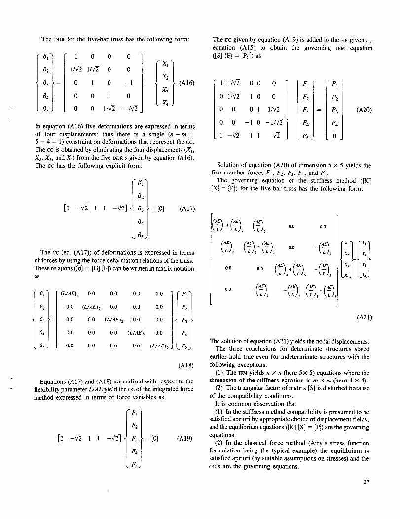
The DDR for the five-bar truss has the following form:
" 81]I
82 II
83 }'----
84
,__sJ
1 0 0
l/x/2- 1/x/-2 0
0 1 0
0 0 1
0 0 1/_/2
0 ] x,
0{tx-1
X30
X4- 1/_/2
(A16)
In equation (A16) five deformations are expressed in terms
of four displacements: thus there is a single (n-m =
5 - 4 = 1) constraint on deformations that represent the cc.
The cc is obtained by eliminating the four displacements (X l,
X 2, X 3, and X4) from the five DDR'S given by equation (A16).
The cc has the following explicit form:
- 8,]
& I
[1 -v_- 1 1 -x/-2] . 8_ _'=[0] (A17)
84 I
_ _sJ
The cc (eq. (A17)) of deformations is expressed in terms
of forces by using the force deformation relations of the truss.
These relations (I8] -- [G] IF]) can be written in matrix notationas
i
• _3 =
_4
(L/AE) 1 0.0 0.0 0.0 0.0
0.0 (L/AE)2 0.0 0.0 0.0
0.0 0.0 (L/AE) 3 0.0 0.0
0.0 0.0 0.0 (L/AE) 4 0.0
0.0 0.0 0.0 0.0 (L/AE)5
"FI"
F2
F3 •
F,
_ F5
(A18)
Equations (A 17) and (A18) normalized with respect to the
flexibility parameter L/AE yield the cc of the integrated force
method expressed in terms of force variables as
[1 -x/2 1 1 -x/_ = [01 (A19)
r- 747372_'1t
rsA
The cc given by equation (A19) is added to the EE given _j
equation (A15) to obtain the governing lrM equation([S] {El = [PI') as
1 1/V_- 0 0 0
0 l/x/2 1 0 0
0 0 0 1 1/_-
0 0 -1 0 -l/x/2
1 -x/2- 1 1 -x/) -
- FI - P1-1i
F2 P2
F3 = P3
I
Fs. OJ
(A20)
Solution of equation (A20) of dimension 5 x 5 yields thefive member forces El, F2, F3, F4, and F5.
The governing equation of the stiffness method ([K]
IX] = IPI) for the five-bar truss has the following form:
xT/, 2-, _-_ o.o o.o
+ 0.0 -, --
2 \L/2 3 _ 3
0.0 0.0 + I - -
4 5 $
0.0 .... +
3 \L/_ 3
-x,]r",l
X'l/"1X,J LP,J
(A21)
The solution of equation (A21) yields the nodal displacements.The three conclusions for determinate structures stated
earlier hold true even for indeterminate structures with the
following exceptions:
(1) The IFM yields n × n (here 5 x 5) equations where the
dimension of the stiffness equation is m × m (here 4 × 4).
(2) The triangular factor of matrix [S] is disturbed because
of the compatibility conditions.It is common observation that
(1) In the stiffness method compatibility is presumed to be
satisfied apriori by appropriate choice of displacement fields,
and the equilibrium equations (IK] IX] = [P]) are the governingequations.
(2) In the classical force method (Airy's stress function
formulation being the typical example) the equilibrium is
satisfied apriori (by suitable assumptions on stresses) and the
cc's are the governing equations.
27

Thequestionis, amongEEandcc whichoneisassumedandwhichoneisenforcedintheintegratedforcemethod?Intheanalysisofindeterminatestructures(refertoIFMgoverningequation[S] IF] = [PI' (eq. (A20) for the indeterminate truss)
both the EE'S and the cc's are simultaneously and explicitly
enforced by the integrated force method. It can be verified
that among the five availabIe methods of structural analysis,
(1) the classical Airy force method, (2) the stiffness method,
(3) the mixed method, (4) the total formulation, and (5) the
integrated force method, only the integrated force method
enforces both EE'S and cc's simultaneously.
The primary IFMvariables are the forces, not a combination
of forces, displacements, and deformations. Therefore theintegrated force method is a direct formulation, and it should
not be confused with the mixed method (in which forces and
displacements are considered as m + n simultaneous primary
unknowns) or with the total formulation (in which forces,
deformations, and displacements are treated as the m + 2n
primary unknowns).
qE
.=
28

Appendix B
Symbols
AI,A2,A3
a,b
03]03]P
[B]R
031,,[B],
[C]
[D]
[O]f
E
e
F
IF]IF] m
f[o][G]e
h
i
[J]
[KI
[K]g
L,e
Lt...L5
_x,My,1%[M]
[Mlf
m
tn o
U_,Uy,Nxyn
n_,ny
IPt
cross-sectional areas of three truss bars
dimension of rectangular element
equilibrium matrix
Prezemieniecki's equilibrium matrix
Robinson's equilibrium matrix
IX equilibrium matrices
compatibility matrix
damping matrix
I_'M damping matrix
Young's modulus
eigen ratio
internal force
force vector of dimension n
force mode shape of dimension n
frequency
flexibility matrix of dimension (n × n)
element flexibility matrix
Hermite polynomials (i,j = 0, 1, 2)
plate thickness
imaginary unity
deformation coefficient matrix of dimension
(m ×m)
stiffness matrix of dimension (m × m)
geometric stiffness matrix of dimension(m X n)
length parameters
lengths of five bars
plate bending moments
mass matrix of dimension (m x m)
lr_ mass matrix
displacement degrees of freedom
lumped mass
membrane stress resultants
force degrees of freedom
direction cosines
mechanical load vector of dimension m
[P]i
Ivl"r
[s]
[Slbt
uc
up/./,V
W
We
XI, X2 ..... XI2
Ix]Ixlm
x,y,z
ol
f3_:
,r
[_RI_R
Ox,Oy
o)
Subscripts:
crt
max, min
Superscript:
T
equivalent loads due to initial imperfections
wM load vector of dimension n
number of compatibility conditions,r=n-m
JFM governing matrix of dimension (n × n)
lF_,l stability matrix
time parameter
complementary strain energy
strain energy
membrane displacement components
transverse displacement
transverse displacement at center
displacement variables
displacement vector of dimension m
displacement mode shape of dimension m
Cartesian coordinates
coefficient of thermal expansion
deformation vector of dimension n
K th deformation component
initial deformation vector
shear strain
effective initial deformation vector
residue in BCC
strain components
rotation about x and y axes
eigenvalue
Poisson's ratio
radian frequency
critical load
maximum or minimum values
transpose of matrix or vector
29

References
1. Patnaik, S.N.: Integrated Force Method Versus the Standard Force
Method. Comput. Struct., vol. 22, no. 2, 1986, pp. 151-163.
2. Patnaik, S.N.: An Integrated Force Method for Discrete Analysis. Int.
J. Numer. Methods Eng., vol. 6, no. 2, 1973, pp. 237-251.
3. Love, A.E.H.: A Treatise on the Mathematical Theory of Elasticity,
Dover, New York, 1944.
4. McGuire, W.; and Gallagher, R.H. : Matrix Structural Analysis. Wiley,
New York, 1979.
5. Gallagher, R.H.; Rattinger, L; and Archer, J.S.: A Correlation Study
of Methods of Matrix Structural Analysis. Agardograph 69, The
MacMillan Co., New York, 1964.
6. Timoshenko, S.: History of Strengths of Material. McGraw-Hill, New
York, 1953.
7. Patnaik, S.N.: The Variational Energy Formulation for the Integrated
Force Method. AIAA J., vol. 24, no. 1, Jan. 1986, pp. 129-137.
8. Whipple, S.: A Work on Bridge Building. Utica, New York, 1847.
9. Stress Recovery at Grid Points, MSC/NASTRAN Applications Manual,
MacNeal-Schwendler Corporation, Los Angeles, CA, 1982, Section 2.2.
I0. Patnaik, S.N.; and Yadagiri, S.: Frequency Analysis of Structures by
Integrated Force Method. J. Sound Vibration, vol. 83, no. 1, July 8,
1982, pp. 93-109.
11. Patnaik, S.N.; and Joseph, K.T.: Compatibility Conditions From
Deformation Displacement Relationship. AIAA J., vol. 23, no. 8, Aug.
1985, pp. 1291-1293.
12. Patnaik, S.N.; and Joseph, K.T.: Generation of the Compatibility Matrix
in the Integrated Force Method. Comput. Methods Appl. Mech. Eng.,
vol. 55, no. 3, May 1986, pp. 239-257.
! 3. Patnaik, S.N.; and Yadagiri, S.! Design for Frequency by the Integrated
Force Method. Comput. Methods Appl. Mech. Eng., vol. 16, no. 2,
Nov. 1978, pp. 213-230.
14. Patnaik, S.N.; and Gallagher, R.H.: Gradients of Behaviour Constraints
and Reanalysis via the Integrated Force Method. Int. J. Numer. Methods
Eng., vol. 23, no. 12, 1986, pp. 2205-2212.
15. Pamaik, S.N.; and Nagaraj, M.S.: Analysis of Continuum by the
Integrated Force Method. Computers Structures, vol. 26, no. 6, 1987,
pp. 899-905.
16. Vijayakumar, K.; Krishna Murty, A.V.; and Pamaik, S.N. : A Basis for
the Analysis of Solid Continua Using the Integrated Force Method. AIAA
J., vol. 26, no. 5, May 1988, pp. 628-629.
17. Przemieniecki, J.S.: Theory of Matrix Structural Analysis. McGraw-
Hill, New York, 1968.
18. Robinson, J.: Integrated Theory of Finite Element Methods. Wiley, New
York, 1973.
19. Gallagber, R.H.: Finite Element Analysis: Fundamentals. Prentice-Hail,
1975.
20. Timoshenko, S.: Theory of Plates and Shells. McGraw-Hill, New York,
1959.
21. Argyris, J.H.: Energy Theorems and Structural Analysis. Butterworth
Scientific Publications, London, 1960.
22. Argyris, J.H.; and Kelsey, S. : The Matrix Force Method of Structural
Analysis With Some New _icat_ons to Aircraft Wings.
ARC-R&M-3034, Aeronautical Research Council, London, Feb. 1956.
23. Argyris, J.H.: ASKA--Automatic System for Kinematic Analysis. Nucl.
Eng. Des., vol. 10, no. 4, Aug. 1969, pp. 441--455.
24. MSC/NASTRAN--NASA Structural Analysis. The MacNeal-Schwendler
Corp., LOs Angeles, CA, 1981.
25. MacNeal R.H.; and Harder, R.L.: A Proposed Standard Set of Problems
to Test Finite Element Accuracy. Finite Elements in Analysis and Design,
vol. 1, no. 1, Apr. 1985, pp. 3-20.
26. Reid, J.K.: Fortran Subroutines for Handling Sparse Linear Programming
Bases. Report AERE-R-8269, Atomic Energy Research Establishment,
1976.
27. Robinson, J.: Automatic Selection of Redundancies in the Matrix Force
Method: The Rank Technique. Canadian Aeronautical J., vol. 11, no. 1,
Jan. 1965, pp. 9-12.
28. Przemieniecki, J.S.; and Denke, P.H.: Joining of Complex Sub-Structures
by the Matrix Force Method. L Airc-raft,voi. 3, no. 3, May-June 1966,
pp. 236-243. _ _
29. Kaneko, I.; Lawo, M.; and Thierauf, G.: On Computational Procedures
for Force Method. Int. J, Numcr, Methods Eng., vol. 18, no. 10, 1982,
pp. 1469-1495.
30. Plemmons, R.J.: A Parallel Block lterative Scheme Applied to
Computations in Structural Analysis. SIAM J. Algebraic Discrete
Methods, vol. 7, no. 3, 1986, pp. 337-347.
31. Heath, M.T.; Plemmons, R.J.; and Ward, R.C.: Sparse Orthogonal
Schemes for Structural Optimization Using the Force Method. SIAM
J. Sci. Slat. Comput., vol. 15, no. 3, Sept. 1984, pp. 514-532.
32. Berke, L. : Optimality 'Criteria Using a Force Method Analysis Approach.
Foundations of Structural Optimization: A Unified Approach, A.J.
Morris, ed., John Wiley & Sons, New York, 1982, pp. 237-269.
33. Fraeijs de Veubeke, B.: Displacement and Equilibrium Models in the
Finite Element Method. Stress Analysis, O.C. Zienkiewicz and G.S.
Holister, eds., John Wiley & Sons, New York, 1965, pp. 145-197.
w
3O


Report Documentation PageNational Aeronaubcs andSpace Administration
1. Report No. 2. Government Accession No. 3. Recipient's Catalog No.
NASA TP-2937
4. Title and Subtitle
Integrated Force Method Versus Displacement Method for Finite
Element Analysis
7. Author(s)
Surya N. Patnaik, Laszlo Berke, and Richard H. Gallagher
9. Performing Organization Name and Address
National Aeronautics and Space AdministrationLewis Research Center
Cleveland, Ohio 44135-3191
12. Sponsoring Agency Name and Address
National Aeronautics and Space Administration
Washington, D.C. 20546-0001
5. Report Date
February 1990
6. Performing Organization Code
8. Performing Organization Report No.
E-4604
t0. Work Unit No.
505-63-1B
11. Contract or Grant No.
13. Type of Report and Period Covered
Technical Paper
14. Sponsoring Agency Code
15. Supplementary Notes
Surya N. Patnaik, National Research Council-NASA Research Associate; Laszlo Berke, Lewis Research Center;
Richard H. Gallagher, Clarkson University, Potsdam, New York 13676.
16. Abstract
A novel formulation termed "the integrated force method" 0FM) has been developed in recent years for
analyzing structures. In this method all the internal forces are taken as independent variables, and the system
equilibrium equations (EE'S) are integrated with the global compatibility conditions (cc's) to form the governingset of equations. In IFM the cc's are obtained from the strain formulation of St. Venant, and no choices of
redundant load systems have to be made, in constrast to the standard force method (SFM). This property of IVM
allows the generation of the governing equation to be automated straightforwardly, as it is in the popular stiffness
method (SM). In this report IFM and SM are compared relative to the structure of their respective equations, their
conditioning, required solution methods, overall computational requirements, and convergence properties as these
factors influence the accuracy of the results. Overall, this new version of the force method produces moreaccurate results than the stiffness method for comparable computational cost.
17. Key Words (Suggested by Author(s))
Finite elements; Integrated force method;
Stiffness method; Flexibility; Compatibility
18. Distribution Statement
Unclassified- Unlimited
Subject Category 39
19. Security Classif. (of this report) 20. Security Classif. (of this page) 21. No of pages
Unclassified Unclassified 36
NASAFORM1626OCT86 *For sale by the National Technical Information Service, Springfield, Virginia 22161
22. Price*
A03
NASA-Langley,1990