integrated geophysical analysis in the northeastern gulf
TRANSCRIPT

University of Nebraska - LincolnDigitalCommons@University of Nebraska - LincolnDissertations & Theses in Earth and AtmosphericSciences Earth and Atmospheric Sciences, Department of
Summer 7-2018
Integrated Geophysical Analysis in theNortheastern Gulf of MexicoMei LiuUniversity of Nebraska-Lincoln, [email protected]
Follow this and additional works at: http://digitalcommons.unl.edu/geoscidiss
Part of the Geology Commons, Geophysics and Seismology Commons, and the Tectonics andStructure Commons
This Article is brought to you for free and open access by the Earth and Atmospheric Sciences, Department of at DigitalCommons@University ofNebraska - Lincoln. It has been accepted for inclusion in Dissertations & Theses in Earth and Atmospheric Sciences by an authorized administrator ofDigitalCommons@University of Nebraska - Lincoln.
Liu, Mei, "Integrated Geophysical Analysis in the Northeastern Gulf of Mexico" (2018). Dissertations & Theses in Earth andAtmospheric Sciences. 109.http://digitalcommons.unl.edu/geoscidiss/109

INTEGRATED GEOPHYSICAL ANALYSIS IN THE NORTHEASTERN GULF
OF MEXICO
By
Mei Liu
A THESIS
Presented to the Faculty of
The Graduate College at the University of Nebraska
In Partial Fulfillment of Requirements
For the Degree of Master of Science
Major: Earth and Atmospheric Sciences
Under the Supervision of Professor Irina Filina
Lincoln, Nebraska
July, 2018

Integrated Geophysical Analysis in the Northeastern Gulf of Mexico
Mei Liu, M.S.
University of Nebraska, 2018
Advisor: Irina Filina
The formation of the Gulf of Mexico (GoM) relates to the breakup of Pangea and
opening of the central Atlantic Ocean. The tectonic history of the basin is still being debated
due to lack of geological constraints. This project addresses the crustal architecture in the
northeastern GoM from integrative analysis of multiple geophysical datasets to provide
constraints for the tectonic reconstruction.
The objectives of this study are: 1) to delineate various tectonic zones (continental
and oceanic domains) and map the boundary between them, 2) to derive physical properties
of the subsurface rocks, 3) to map the major tectonic structures in the study area, such as
the pre-salt basin and the Seaward Dipping Reflectors (SDR) province in continental
domain, and segments of an extinct spreading center with associated transform faults in
oceanic domain, and 4) to establish the spatial and temporal relations between different
tectonic zones and structures.
Three two-dimensional subsurface models were developed in the northeastern
GoM by using consistent physical properties for subsurface rocks. Further, spatial analysis

was performed on gravity and magnetic grids, which allowed mapping of various tectonic
zones and structures.
As a result of this study, two distinct spreading episodes of GoM formation were
identified. The first one, presumably from 160 to 150 Ma, was an ultra-slow spreading
event (estimated full spreading rate of 0.9 cm/yr) that produced thin (~5 km) and dense
(2.95 g/cc) oceanic crust with fast seismic velocities (~7km/s) and high magnetic
susceptibility (0.0075 cgs), most likely composed of gabbro. At ~150 Ma, the spreading
center jumped to the south due to a change in location of the Euler pole. The second
spreading episode was faster (1.1 cm/yr) and produced thicker crust (up to 9 km) composed
of two layers – a basaltic layer (2-4 km thick, Vp = 6-6.5 km/s, density 2.65 g/cc and
magnetic susceptibility 0.007 cgs) on top of a gabbroic one. The ridge propagation resulted
in the asymmetry of the oceanic domain that needs to be accounted for during tectonic
reconstruction.

i
Dedication
This thesis is firstly dedicated to my parents, Yilin Liu and Guangyu Shao.
My mother has taught me how to be an independent woman with courage and love. My
father used his patience and intelligence taught me the virtues of persistence. I would like
to thank them for providing me the opportunity to study abroad even though they have
never been to the U.S. before. I also would like to thank them for always being proud of
me. My parents read this thesis over and over again even though they have to rely on a
dictionary to understand English. These words could never express my gratitude and thanks
to my beloved parents.
This work is also dedicated to my grandparents, the rest of my family, and my
friends. It is your kindness, enthusiasm towards life, and love motivated me to be a better
person.
Last but not least, this thesis is dedicated to Jesse A. Ash who has accompanied me
through every effort of this thesis and provides me endless encouragement.

ii
Acknowledgements
I would like to acknowledge several people have contributed to make this thesis
possible. First of all, I would like to thank my advisor, Dr. Irina Filina, for her guidance
and mentorship on this project. Her knowledge, patience, and enthusiasm pushed my work
to where it is. I would not be able to have this achievement without her kindly assistance.
I would also like to acknowledge Dr. Chris Fielding and Dr. Caroline Burberry for serving
on my committee. Dr. Mindi Searls who provided a lot of valuable feedback on my work
during our weekly meetings.
In addition, I would like thank Dr. Erin Betuel who has provided incredible ideas
to inspire me on this project.
Lastly, I would like to acknowledge the UNL Department of Earth and Atmospheric
Sciences for the financial support and numerous other professors and students for their
kindness support and friendship. Thank you very much!

iii
Table of Contents
List of Figures v
List of Tables vii
CHPATER 1. Introduction to the Study Area 1
1.1 Motivation for the study 1
1.2 Tectonic history of the Gulf of Mexico 7
1.3 Stratigraphy in the northeastern Gulf of Mexico 13
CHAPTER 2. Geophysical Data 16
2.1 Seismic refraction data 16
2.2 Seismic reflection data 21
2.3 Gravity data 30
2.4 Magnetic field 33
2.5 Bathymetry 35
2.6 Earthquakes in the northeastern GoM 35
2.7 Well data 39
CHAPTER 3. Integrated Geophysical Modelling 42
3.1 Models 1A and 1B 42
3.2 Model 2 50
3.3 Model 3 53
Chapter 4. Spatial Analysis of Gravity and Magnetic Fields 60
4.1 Filtering of potential fields 60

iv
4.2 Correlation with 2D subsurface models 63
4.3. Combined Interpretations of the Tectonic Structures in the Study Area 65
4.4 Validation of interpreted geological structures with the literature 67
CHAPTER 5 Discussion 72
5.1 Observations from this study 72
5.2 The ridge jump in literature 73
5.3 Propagating ridge in the GoM 78
CHAPTER 6. Conclusion 87
Reference 89

v
List of Figures
Figure 1 ............................................................................................................................... 1
Figure 2 ............................................................................................................................... 3
Figure 3 ............................................................................................................................... 7
Figure 4 ............................................................................................................................. 15
Figure 5 ............................................................................................................................. 17
Figure 6 ............................................................................................................................. 18
Figure 7 ............................................................................................................................. 19
Figure 8 ............................................................................................................................. 21
Figure 9 ............................................................................................................................. 22
Figure 10 ........................................................................................................................... 25
Figure 11 ........................................................................................................................... 26
Figure 12 ........................................................................................................................... 27
Figure 13 ........................................................................................................................... 27
Figure 14 ........................................................................................................................... 28
Figure 15 ........................................................................................................................... 29
Figure 16 ........................................................................................................................... 30
Figure 17 ........................................................................................................................... 31
Figure 18 ........................................................................................................................... 32
Figure 19 ........................................................................................................................... 33
Figure 20 ........................................................................................................................... 34
Figure 21 ........................................................................................................................... 36
Figure 22 ........................................................................................................................... 40

vi
Figure 23 ........................................................................................................................... 44
Figure 24 ........................................................................................................................... 48
Figure 24 ........................................................................................................................... 48
Figure 25 ........................................................................................................................... 51
Figure 26 ........................................................................................................................... 54
Figure 27 ........................................................................................................................... 61
Figure 28 ........................................................................................................................... 62
Figure 29 ........................................................................................................................... 64
Figure 30 ........................................................................................................................... 66
Figure 31 ........................................................................................................................... 68
Figure 32. .......................................................................................................................... 69
Figure 33 ........................................................................................................................... 70
Figure 34 ........................................................................................................................... 74
Figure 35 ........................................................................................................................... 76
Figure 36 ........................................................................................................................... 77
Figure 37 ........................................................................................................................... 79
Figure 38 ........................................................................................................................... 81
Figure 39 ........................................................................................................................... 82
Figure 40 ........................................................................................................................... 83
Figure 41 ........................................................................................................................... 84
vii
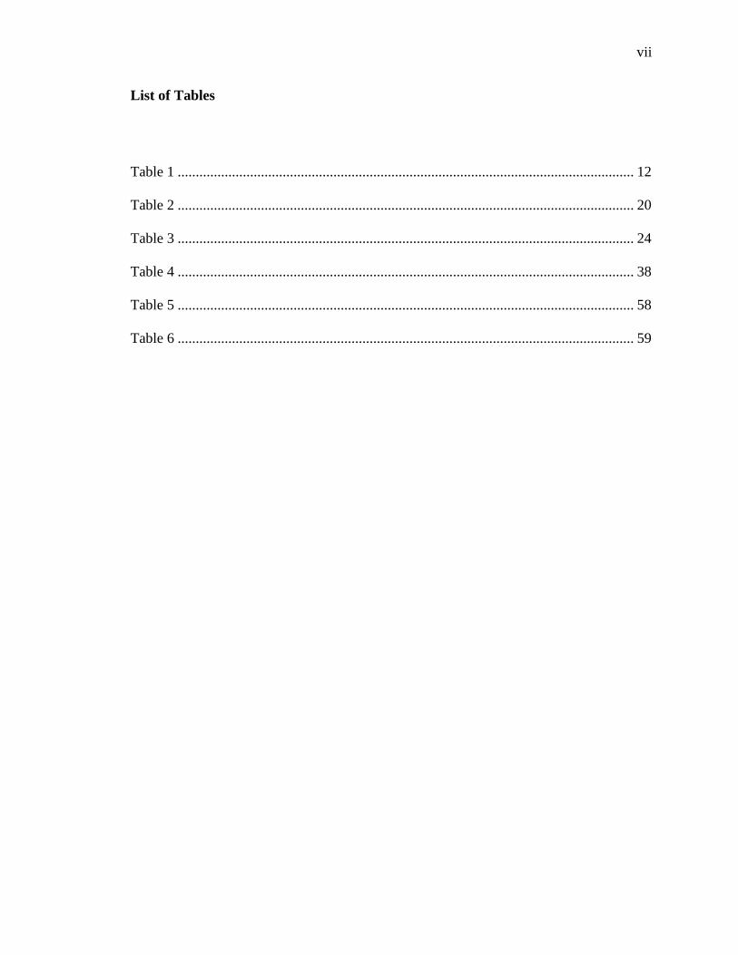
List of Tables
Table 1 .............................................................................................................................. 12
Table 2 .............................................................................................................................. 20
Table 3 .............................................................................................................................. 24
Table 4 .............................................................................................................................. 38
Table 5 .............................................................................................................................. 58
Table 6 .............................................................................................................................. 59
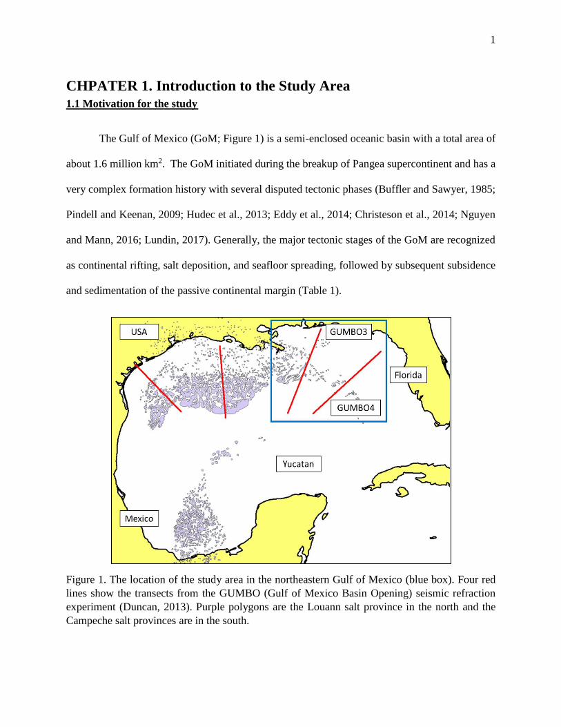
1
CHPATER 1. Introduction to the Study Area
1.1 Motivation for the study
The Gulf of Mexico (GoM; Figure 1) is a semi-enclosed oceanic basin with a total area of
about 1.6 million km2. The GoM initiated during the breakup of Pangea supercontinent and has a
very complex formation history with several disputed tectonic phases (Buffler and Sawyer, 1985;
Pindell and Keenan, 2009; Hudec et al., 2013; Eddy et al., 2014; Christeson et al., 2014; Nguyen
and Mann, 2016; Lundin, 2017). Generally, the major tectonic stages of the GoM are recognized
as continental rifting, salt deposition, and seafloor spreading, followed by subsequent subsidence
and sedimentation of the passive continental margin (Table 1).
Figure 1. The location of the study area in the northeastern Gulf of Mexico (blue box). Four red
lines show the transects from the GUMBO (Gulf of Mexico Basin Opening) seismic refraction
experiment (Duncan, 2013). Purple polygons are the Louann salt province in the north and the
Campeche salt provinces are in the south.

2
According to the published models, the continental rifting initiated in the Late
Triassic (230 Ma, Pindell and Keenan, 2009; Hudec et al., 2013; Eddy et al., 2014; Christeson et
al., 2014; Nguyen and Mann, 2016; Lundin, 2017) and provided the accommodation for deposition
of the pre-salt sediments, such as the Eagle Mill Formation in the northern GoM (Pilger, 1981;
Warwick, 2017) and the La Boca Formation in Mexico (Bartok, 1993). Thick salt was deposited
in a short time interval in the Callovian (~166-163Ma, Salvador, 1991). The presence of multiple
complex salt bodies in the sedimentary section obscures seismic imaging and challenges the study
of the crustal structures within the basin. The oceanic crust formed in the Jurassic (160-140 Ma,
Eddy et al., 2014) during the counterclockwise rotation of the Yucatan crustal block, leaving
behind a series of extinct spreading segments offset by transform faults. As the formation of the
Gulf of Mexico is closely related to the opening of the central Atlantic Ocean, any tectonic
reconstruction of Pangea requires thorough understanding of the GoM’s complex history.
However, the pre-breakup location of the Yucatan block is still not well constrained. This study
aims to provide important constraints for the basin restoration, such as the location of the Seaward
Dipping Reflectors (SDRs) and pre-salt sedimentary provinces as they are supposed to match on
the conjugate margins.
Many tectonic models have been developed for the GoM (Buffler and Sawyer, 1985;
Pindell, 1985; Marton and Buffler, 1994; Kneller and Johnson, 2011; Hudec et al., 2013; Pindell
and Keenan, 2009; Christeson et al., 2014; Nguyen and Mann, 2016, Lundin 2017). However, the
location of the key tectonic structures, such as the ocean-continent boundary (OCB) and extinct
spreading centers with associated transform faults, are still being debated (Figure 2). The published
studies shown in Figure 2 were performed based on one or two geophysical methods. For example,
Sandwell et al. (2014) and Nguyen and Mann (2016) mapped the tectonic structures based on

3
satellite gravity. Interpretations of Hudec et al. (2013) are based on seismic data. Pindell et al.
(2016) used aeromagnetic data to determine the location of key tectonic structures. This study
integrated all publically available geophysical datasets: multiple seismic refraction and reflection
surveys, well logs, gravity and magnetic data.
Figure 2. a) Location of the ocean-continent boundary (OCB) from various publications in the
Gulf of Mexico. b) Location of published extinct spreading ridges and transform faults. The purple
dot is the pole of rotation from Nguyen and Mann, 2016. The black dot is the pole of rotation from
Pindell and Keenan, 2009. The background is vertical gravity gradient from Sandwell et al., 2014.
Figure 2 suggests striking asymmetry in the oceanic domain in the study area. The oceanic
zone to the north of the spreading center is dramatically wider than the one to the south. This was
noted by some of the authors (Hudec et al., 2013; Nguyen and Mann, 2016), but none of the
previously published models discussed the reasons for such an asymmetric spreading in the GoM.
This study addresses the observed high degree of asymmetry in the basin and proposes a
mechanism to explain this observation in the northeastern GoM.
The Gulf of Mexico Basin Opening project (GUMBO, Duncan, 2013) provided new
constraints on the structure of continental and oceanic crust in the northern part of the basin. The

4
four profiles of the GUMBO project targeted the northwestern (GUMBO Line 1), central
(GUMBO Line 2), and eastern U.S. GoM (GUMBO Line 3 and GUMBO Line 4), as shown in
Figure 1. Two recently published papers (Eddy et al., 2014; Christeson et al., 2014) presented the
results of seismic refraction experiments along lines GUMBO3 and GUMBO4 in the northeastern
GoM, featuring two distinct crustal zones in the oceanic domain. To date, none of the tectonic
models have addressed the dramatic variations in crustal thickness and physical properties. This
study provides an explanation for observed lateral variations in the oceanic crust and ties these
distinct crustal zones to different spreading episodes.
The GoM comprises one of the largest petroleum provinces in the world (Whaley, 2006;
Galloway, 2009). The first oil was extracted from the GoM back in 1938 (Galloway, 2009). In
2016, the total GoM production was around 4.5 MMboepd, with 80% liquid content (Erlingsen,
2017). According to the National Outer Continental shelf (OCS) program, the estimated resources
on 160 million acres of the US sector contain about 48 Bbbl of undiscovered technically
recoverable oil and 141 Tcf of undiscovered technically recoverable gas (WorldOil website,
http://www.worldoil.com/news/2018/4/2/boem-announces-date-for-gulf-of-mexico-lease-sale-
251). Despite the long exploration history, the GoM still contains huge hydrocarbon potential. In
addition, the environmental regulation is the strictest in the northeastern GoM and the federal law
bars drilling within 125 miles of Florida’s Gulf coast (Henry, 2017). Therefore, the study area has
received less attention from the petroleum industry than the rest of the US sector of the basin. This
study provides important geological constraints on the tectonic architecture and crustal parameters
of the northeastern GoM that are crucial for the petroleum basin modeling that guides hydrocarbon
exploration.

5
Hartford and Filina (2018) performed similar integrative analysis of various geophysical
datasets in the southern GoM and mapped the extend of the pre-salt basin along the Yucatan
margin, where the pre-salt sediments are confidently imaged (Williams-Rojas et al. 2011;
Sounders et al., 2017; O’Reily et al., 2017). As pre-salt petroleum exploration has gained extreme
success in other basins, such as the Santos basin in Brazil (Diaz, 2018) and Kwanza basin in West
Africa (Koning, 2014), pre-salt plays are emerging in the GoM (Arbouille et al., 2013). However,
there are not many publically available seismic data over the pre-salt basin in the northeastern
GoM. This study uses an integrative approach that combines multiple geophysical and geological
datasets in order to determine the spatial extent and the thickness of the pre-salt deposits in the
northeastern GoM. These are not only important for petroleum exploration, but also can be used
to constrain the tectonic reconstruction of the entire basin, as they should match on the conjugate
margins.
In addition, several crustal earthquakes (with the focal depths below 14 km) occurred in
the middle of the oceanic domain in the study area, but far away from known tectonic structures.
No current tectonic model takes these into consideration although these are large magnitude events
(4.9 – 5.9 on the Richter’s scale). The focal mechanisms developed for two of these earthquakes
suggest compressional stress released along faults that do not correlate with any spreading centers
or transform faults. Our study ties the observed seismicity in the northeastern GoM with a zone of
weakness (pseudofault) between two distinct oceanic domains resulted from two spreading
episodes.
The overarching goal of this study is to better understand the tectonic history of the Gulf
of Mexico and provide an explanation for the several geological and geophysical observations that
are not explained by any published tectonic model. These include known dramatic variations in

6
thickness and physical properties of the oceanic crust, the location of the ocean-continent boundary
(Figure 2a), the location of extinct spreading ridges (Figure 2b), the apparent large degree of
spreading asymmetry of the basin, noted by some authors, but not yet explained, and the
mysterious crustal earthquakes in the center of the basin that are not aligned with any known
geological structures.

7
1.2 Tectonic history of the Gulf of Mexico
Although the tectonic history of the GoM has been debated over decades (Buffler and Sawyer,
1985; Pindell and Keenan, 2009; Hudec et al., 2013; Eddy et al., 2014; Christeson et al., 2014;
Nguyen and Mann, 2016; Lundin, 2017), most researchers agree that the opening of the Gulf of
Mexico basin generally includes three stages as is shown in Figure 3:
Figure 3. Brief tectonic
history of the Gulf of Mexico
modified from Eddy et al.,
2014. Four red lines are four
seismic refraction profiles
(GUMBO1-4).
a) Stage 1: NW-SE
continental rift, marked by
black arrows. YB-Yucatan
Block.
b) Stage 2: salt deposits
started accumulating in the
stretched continental region.
The direction of continental
rift changed from NW-SE to
N-S.
c) Stage 3: the Yucatan block
rotated counterclockwise
away from North America
plate during seafloor
spreading and formed the
GoM basin. Seafloor
spreading ceased in the Early
Cretaceous. Arrows indicate
the rifting direction. YB-
Yucatan Block. OC- Oceanic
crust. ESR-Extinct spreading
ridge. Plus symbols are the
Gulf coast magnetic
anomaly.

8
Stage 1: Continental rifting (Late Triassic-Middle Jurassic, 230 – 158 Ma)
The first stage comprises a continental rift in the Late Triassic to Middle Jurassic (230-
158 Ma) between the Yucatan block, North America, and South America (Pindell and Keenan,
2009; Hudec et al., 2013; Eddy et al., 2014; Christeson et al., 2014; Nguyen and Mann, 2016;
Lundin, 2017). However, the exact timing is still under debate (Table 1). Pindell (1985) proposed
the rifting happened between 190 and 158 Ma, while Hudec et al. (2013) suggested that the rifting
occurred between 240 and 166 Ma (Table 1). It is believed that this initial continental rift was
caused by northwest-southeast stretching (Pindell and Keenan, 2009; Hudec et al., 2013; Eddy et
al., 2014; Nguyen and Mann, 2016). The red beds, such as the Eagle Mill formation in the
northeastern GoM and its equivalents (La Boca Formation) filled the extensional grabens in the
rifting stage (Bartok, 1999; Hudec et al., 2013). Mickus et al. (2009) proposed that continued
rifting formed a volcanic rifted margin in the northwestern part of the basin, resulting in seaward-
dipping seismic reflectors (SDRs) along the Gulf coast. This conclusion is based on the presence
of a pronounced magnetic anomaly along the Texas coastline, known as the Houston magnetic
anomaly after Hall (1990). Volcanic rifted margins usually are formed by rapid, voluminous
emplacement of lavas, dikes, sills, and plutons (Mickus et al., 2009). Pascoe et al. (2016) believe
the volcanic margin interpretation is unlikely and suggest that the zone of high magnetic intensity
represents a suture zone related to the late Paleozoic orogeny during formation of Pangea. A similar
interpretation was proposed by Kneller and Johnson (2011) and Van Avendonk et al. (2015), who
concluded that the rifting was volcanic-poor and resulted in a mantle exhumation in the
northwestern GoM. Eddy et al. (2014) suggest that the SDRs along the eastern GoM margin,
coincident with magnetic highs, may be a part of an “inner wedge” system of syn-rift basins, filled
with basalts and volcaniclastic sediments during continental extension.

9
Stage 2: salt deposition (Late Jurassic, ~158 Ma)
This stage includes a short period of widespread deposition of a thick salt layer that filled
in the Proto-GoM basin. Some researchers believe that this was associated with the final stage of
continental rifting, so the salt was deposited on the stretched continental crust (Pindell, 1985; Bird,
2005; Galloway, 2009; Pindell and Keenan, 2009; Nguyen and Mann, 2016). According to Hudec
et al. (2013), continental rifting continued another 2 Ma after the salt was deposited. However, a
number of models allow salt deposition on oceanic crust (Stern and Dickson, 2010; Padilla-
Sanchez, 2017). Consequently, the origin and timing of salt deposition is still being debated (Table
1). According to Bird et al. (2005), before the sea-floor spreading (next tectonic stage), the Yucatan
block rotated about 22 degrees counterclockwise between 160 Ma and 150 Ma (as a part of
continental rifting), which allowed intermittent seawater influx and produced massive salt
deposition. Dribus et al. (2008) proposed that storm surges from the Pacific entering the Proto-
GoM and eventually forming the evaporites. Pindell and Keenan (2009) suggested the salt was
deposited before the Late Callovian (158 Ma). According to Hudec et al. (2013), an evaporite sump
was isolated from the world ocean and became saline enough to deposit halite between 165 and
161 Ma (Callovian).
Nevertheless, the relationship and timing between the salt and the oceanic crust are still
unclear. Padilla-Sanchez (2017) proposed that the salt was deposited after the oceanic crust (next
stage) was already formed and ceased, i.e. the basin was opened before the salt was deposited.
This study accepts the timing proposed by the majority of the models and assumes that the salt
formed on the stretched continental crust before the seafloor spreading commenced.

10
Stage 3: Seafloor spreading and rotation of the Yucatan Block (Late Jurassic to Early Cretaceous,
162-130 Ma)
Some authors (Stern and Dickinson, 2010, Lundin, 2017) proposed that the GoM is a
backarc basin (BAB, a basin formed via seafloor spreading behind an active subduction zone).
According to Stern and Dickinson (2010), the GoM opened behind the 232-150 Ma old Nazas arc
over an east-dipping subduction zone in Late Jurassic time, beginning ca. 165 Ma. The spreading
ridges in the oceanic domain of the GoM are oriented nearly orthogonally to the Paleo-Pacific
subduction direction (Stern and Dickinson, 2010; Lundin, 2017).
The exact time when the oceanic crust formed and whether the salt was formed on the
oceanic crust or flowed later onto oceanic crust is still being debated (Table 1). Although the
timing, the initial location of the Yucatan, the angle of rotation, and the relationship with salt are
still not well constrained, there is overall agreement that the oceanic crust in the GoM formed
while the Yucatan crustal block rotated counterclockwise from North America. According to
Pindell and Keenan (2009), the seafloor spreading initiated in the very early Oxfordian age
(158 Ma). According to Eddy et al. (2014), between Jurassic to Early Cretaceous(~152-132Ma),
the Yucatan Block rotated about 40 degrees counterclockwise away from the North American
plate, which lead to a separation of the initial salt basin into the northern Louann and the southern
Campeche salt provinces (Figure 1).
Published tectonic reconstruction models have proposed different locations of the Euler
pole, as well as various rotation angles for the Yucatan crustal block (Table 1). The proposed total
angle of rotation is 43 degrees according to Pindell (1985), 37 degrees according to Nguyen and
Mann (2016), and 78+/- 11 degrees according to Lundin (2017). The pole of rotation is located in
11
the region defined by the following coordinates at 79-84 °W, 23-30 °N (Bird et al., 2005; Pindell
and Keenan, 2009; Stern and Dickson, 2010; Nguyen and Mann, 2016).
Most of the tectonic models suggest that the oceanic crust formation started in the western
GoM and propagated to the east (Christeson et al., 2014; Eddy et al., 2014; Pindell and Kennan,
2009; Nguyen and Mann, 2016; Lundin 2017). This conclusion is guided by generally accepted
tectonic reconstruction with the Euler pole located in the region between the Florida Straits and
Northern Cuba as described above. In contrast, Hudec et al. (2013) concluded that seafloor
spreading started simultaneously in the western and eastern parts of the basin and propagated
toward to the center of the basin based on analysis of multiple proprietary seismic datasets in all
parts of the GoM.
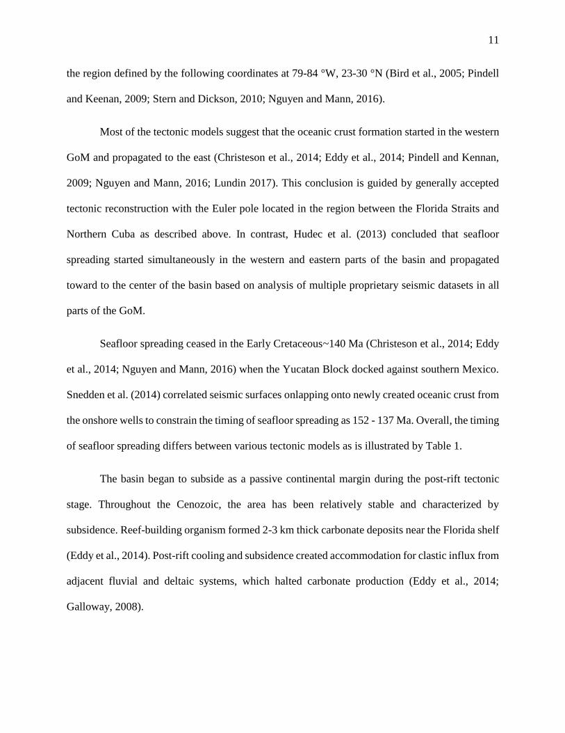
Seafloor spreading ceased in the Early Cretaceous~140 Ma (Christeson et al., 2014; Eddy
et al., 2014; Nguyen and Mann, 2016) when the Yucatan Block docked against southern Mexico.
Snedden et al. (2014) correlated seismic surfaces onlapping onto newly created oceanic crust from
the onshore wells to constrain the timing of seafloor spreading as 152 - 137 Ma. Overall, the timing
of seafloor spreading differs between various tectonic models as is illustrated by Table 1.
The basin began to subside as a passive continental margin during the post-rift tectonic
stage. Throughout the Cenozoic, the area has been relatively stable and characterized by
subsidence. Reef-building organism formed 2-3 km thick carbonate deposits near the Florida shelf
(Eddy et al., 2014). Post-rift cooling and subsidence created accommodation for clastic influx from
adjacent fluvial and deltaic systems, which halted carbonate production (Eddy et al., 2014;
Galloway, 2008).

12
Tab
le 1
. S
um
mar
y o
f pu
bli
shed
tec
tonic
model
s fo
r th
e G
ulf
of
Mex
ico.

13
1.3 Stratigraphy in the northeastern Gulf of Mexico
The sediments in the northeastern GoM consist of siliciclastics, carbonates, and salt (Galloway,
2009). The age of the sedimentary rocks spans from Late Triassic up to recent (Figure 4). During
the first stage of the rifting in the Late Triassic, volcanic clasts and redbeds filled in the grabens
developed on the stretched crust, forming the Eagle Mill Formation in the northern part (Pilger,
1981; Warwick, 2017) and La Boca Formation (Bartok, 1999) in the southern part, which are the
pre-salt deposits. Goswami et al. (2017) suggest a largely clastic lithology with minor amounts of
interbedded volcanics in the pre-salt package. The consequent marine transgression led to marine
water being trapped in the basin, resulting in deposition of the Werner Anhydrite Formation
(Salvador, 1987). During periods of marine influx and evaporation, the Louann salt was deposited
in the basin (Salvador, 1991). The time of salt deposition differs slightly between the models
(Table 1). Wilson (2011) believes the Louann salt was deposited in the basin from Bajocian to
Callovian (~167 to 162 Ma, but an exact age was not provided in the text rather estimated from
the International Chronostratigraphic Chart), while Pindell (1985) suggest the Louann salt was
deposited in the basin around the Callovian (158 Ma). According to Wilson (2011), during the
Early Oxfordian (~160Ma, Late Jurassic), texturally mature aeolian sands were deposited in the
northeastern GoM basin forming the Norphlet Formation. These aeolian quartzose sandstone
facies consist of well-rounded, well-sorted, quartz-rich, hematite-coated sands, deposited with
little to no clay matrix during a Late Jurassic transgression, are also reported by Pearson (2011)
and Steier (2018). The Norphlet Formation is one of the critical reservoir rocks in the northeastern
GoM and is producing in present-day Mississippi, Alabama, Florida, and the deep water
northeastern GoM (Godo, 2017; Steier, 2018). In Oxfordian time (~156 Ma, Late Jurassic), another
marine transgression formed the carbonate unit, known as the Smackover Formation (Wilson,

14
2011), which is the primary source rock in the northeastern GoM. The sea level continued to rise,
and the Haynesville Formation, consisting of sandstone, siltstone, and shales was deposited in the
eastern Gulf region during the Kimmeridgian (~152 Ma, Salvador, 1987) time. At the beginning
of the Early Cretaceous (~150 Ma), the Cotton Valley Formation formed as a primary reservoir
and was intimately interbedded with source rocks in the northern GoM (Galloway, 2009). The end
of the Cotton Valley Formation indicates the beginning of the modern carbonate platform
accumulation (Wilson, 2011). Rimmed carbonate shelf developed during Cretaceous (Galloway,
2008). Paleogene clastic progradation resulted in the deposition of the following formations
(Figure 4): Midway, Wilcox, Claiborne, Jackson, Vicksburg, and Catahoula formations. Among
these formations, Wilcox group comprises a major reservoir in the northern GoM and
characterized as fluvial, deltaic, and shallow marine environment (Fisher and McGowen, 1976).
The Fleming group was deposited as a result of Miocene progradation in the central and
northeastern Gulf (Galloway, 2008). The Neogene deposits progradated in the basin along the
central Gulf margin, while a primarily aggradational carbonate platform formed along the Florida
margin (Galloway, 2008).

15
Figure 4. Stratigraphy of the northeastern
Gulf of Mexico modified from Warwick,
2017.

16
CHAPTER 2. Geophysical Data
2.1 Seismic refraction data
In 2010, the Gulf of Mexico Basin Opening Project (GUMBO) was conducted to study the
lithological composition and structural evolution of the GoM (Duncan, 2013; Eddy et al., 2014;
Christeson et al., 2014). It used Ocean Bottom Seismometers (OBS) and an air-gun seismic source
to collect seismic refraction data in the U.S. Gulf along four profiles (Figure 1): GUMBO1 in the
northwestern GoM, GUMBO2 in the center, and GUMBO3 and 4 in the northeastern GoM. The
length of GUMBO transects ranges from ~300 km to over 500 km. The OBS spacing for transects
in the eastern GoM is 12 km with a time sampling interval of 5 ms and a shot spacing of 150 m
(Duncan, 2013).
GUMBO3 (Figure 5) extends from offshore Florida, across De Soto Canyon, to the center
of the basin. The total length of GUMBO3 is 524 km. Figure 5 shows the interpretation of seismic
refraction data from Eddy et al., 2014. The three layers are defined based on velocity structure,
which are sediments, crust, and mantle. Eddy et al. (2014) also interpreted a carbonate platform
and several salt structures in this line. The line starts in the continental domain and ends in the
oceanic domain with the OCB interpreted by Eddy et al. (2014) to be at the distance of 270-290 km.
The top of the continental crust is at a depth of ~7 km, which is shallower than oceanic crust at
~ 10 km. The continental crust at the beginning of the profile is ~25 km thick, while the oceanic
crust has an average thickness of ~9 km. The oceanic crust near the OCB is thinner (8 km) and its
thickness increases to 10 km at 430 km along model distance. The velocity of the upper oceanic
crust varies between 6 km/s to 6.5 km/s, while the velocity of the lower oceanic crust is 6.5 to
7 km/s.
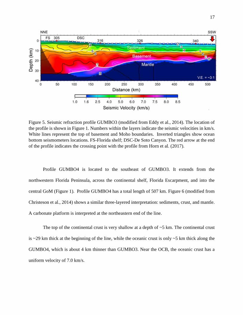
17
Figure 5. Seismic refraction profile GUMBO3 (modified from Eddy et al., 2014). The location of
the profile is shown in Figure 1. Numbers within the layers indicate the seismic velocities in km/s.
White lines represent the top of basement and Moho boundaries. Inverted triangles show ocean
bottom seismometers locations. FS-Florida shelf; DSC-De Soto Canyon. The red arrow at the end
of the profile indicates the crossing point with the profile from Horn et al. (2017).
Profile GUMBO4 is located to the southeast of GUMBO3. It extends from the
northwestern Florida Peninsula, across the continental shelf, Florida Escarpment, and into the
central GoM (Figure 1). Profile GUMBO4 has a total length of 507 km. Figure 6 (modified from
Christeson et al., 2014) shows a similar three-layered interpretation: sediments, crust, and mantle.
A carbonate platform is interpreted at the northeastern end of the line.
The top of the continental crust is very shallow at a depth of ~5 km. The continental crust
is ~29 km thick at the beginning of the line, while the oceanic crust is only ~5 km thick along the
GUMBO4, which is about 4 km thinner than GUMBO3. Near the OCB, the oceanic crust has a
uniform velocity of 7.0 km/s.

18
Toward the end of the profile, the velocity of the top 2.5 km of the oceanic crust drops to
6.0 km/s and to 6.8 km/s in the lower portion of the oceanic crust. Notably, these two profiles are
~125km away from each other, but they show dramatic variations in the oceanic crust, namely in
the crustal thickness and the velocity of compressional seismic waves.
Figure 6. Seismic refraction profile GUMBO4 (modified from Christeson et al., 2014). The
location of the profile is in Figure 1. Refer to Figure 5 for description.
Several vintage seismic refraction points from Ibrahim et al. (1981) were used to validate
the depth of basement and the Moho (Table 2) in the study area. The distribution of seismic
refraction points is shown in Figure 7.

19
Figure 7. Location of seismic refraction points from Ibrahim et al. (1981) in the study area. The
data are listed in Table 2. The three profiles were used to build 2D subsurface models.

20
Tab
le 2
. S
eism
ic r
efra
ctio
n d
ata
from
Ib
rahim
et
al.,
1981.
See
Fig
ure
7 f
or
loca
tion o
f th
ese
refr
acti
on
pro
file
s.

21
2.2 Seismic reflection data
There are seismic reflection profiles along GUMBO3 and 4 transects. Profile Fugro533
(Figure 8) overlaps with GUMBO3 (Eddy et al., 2014). The top of the basement and Moho (blue
and black lines in Figure 8) are interpreted from the GUMBO3 refraction experiment. Salt
structures are located at the model distance of ~170 to 310 km in the sedimentary unit (Eddy et al.,
2014). Reflectors in the basement beneath the salt structures are observed with seaward dips of
~25°-30°, which are interpreted as volcanic seaward dipping reflectors (SDRs) (Eddy et al., 2014).
The SDR layer under the Apalachicola Basin has a width of 100 km and a depth of ~10 km.
Toward the end of the line, an extinct spreading ridge (ESR) is interpreted to be coincident
with the observed half-graben structure from Eddy et al. (2014). Near the OCB, at the distance of
300-400 km along the model, the Moho from GUMBO3 is interpreted at depth of 23 km. However,
there are strong reflectors at a depth of ~17.98 km in the refraction seismic that could also be
interpreted as the Moho (shown with arrows in Figure 8).
Figure 8. Seismic reflection profile Fugro533 (modified from Eddy et al., 2014). The location of
this profile is the same as GUMBO3. The blue line and black line denotes the top of the basement
and Moho interpreted from GUMBO3 respectively. The red arrow indicates an alternative Moho
reflector. AB-Apalachicola Basin; B-MCS Basement; C-carbonate platform; DSC-De Soto
Canyon; ESR- extinct spreading ridge; LDR- landward dipping reflector; SDR-seaward dipping
reflector; SP-Southern Platform.

22
Seismic reflection profile Fugro642 (Figure 9) overlaps with GUMBO4. The top of the
basement seismic reflectors is not associated with strong contrast due to the thick carbonate
platform, which tends to attenuate the signal of deep reflectors (Christeson et al., 2014). In the
deep-water region, there are no significant basement reflections observed, nor is there a clear
landward dipping basement ramp as in GUMBO3 (Christeson et al., 2014).
Figure 9. Seismic reflection profile along Fugro642 (Modified from Christeson et al., 2014). The
dark blue denotes the top of the basement. White arrows mark strong reflectors. ESR—extinct
spreading center. ESR is detected from potential fields and Vp (~6 km/s). Close-up of MoR1is
shown in Figure 26.
Table 3 shows the comparison of depths to basement and Moho from different sources.
The vintage refraction data (location is in Figure 7) suggest ~3-4 km shallower basement than both
GUMBO3 and Fugro533 (Table 3). In terms of Moho depth, Fugro533 is in agreement with
seismic refraction points (Table 3), while GUMBO3 suggests a ~2 km deeper Moho interpretation.
Thus, the vintage refraction data agrees better with seismic reflection data (Fugro533) than with
the seismic refraction line (GUMBO3). These two alternative Moho interpretations led to two
subsurface models developed for profile GUMBO3: Model 1A for seismic refraction data (deep
Moho), and Model 1B for seismic reflection data (shallow Moho). Since the basement and Moho

23
interpretations are in agreement between GUMBO4 and Fugro642 profiles, only one subsurface
model was developed for that line - Model 2.

24
Tab
le 3
. D
epth
to d
iffe
rent
geo
logic
al b
oundar
ies
in k
m f
rom
dif
fere
nt
seis
mic
ex
per
imen
ts.

25
Several additional 2D and 3D seismic reflection surveys were used to validate the basement
structures and to constrain subsurface modeling. The locations of those are shown in Figure 10.
Figure 10. Seismic data used in this project. G3 and G4 are two GUMBO profiles from the Gulf
of Mexico Basin Opening project. Gray box outlines 3D seismic reflection survey from Deighton
et al., 2016. Two green dots indicate the well locations from the Bureau of Ocean Energy
Management website (BOEM). Well No Logs G2468 is next to GUMBO3 and well No. 1 O.C.S.-
G-2516 is located on GUMBO4. Several blue dots indicates the seismic refraction database from
Ibrahim et al., 1981.
The line from Saunders et al., 2016 (thin purple line in Figure 10) partially overlaps
GUMBO3. The seismic reflection image for that line is shown in Figure 11. The basement

26
structures are well imaged in this profile. It was used to validate the location of the extinct
spreading center (mid-ocean valley).
Figure 11. Seismic reflection profile from Saunders et al., 2016. The vertical scale is two-way
travel time in seconds. The yellow line on the right side of the profile is the well in the block Lloyd
ridge 399. The horizontal line bar on the top indicates part of the profile that overlaps with
GUMBO3 profile (Figure 5). The black box outlines the extinct spreading center.
Figure 12 shows another 2D seismic reflection line used for subsurface modeling. Model 3
was developed along the line acquired by ION in 2015 (Horn et al., 2017). This line starts near
GUMBO4, and it crosses GUMBO3 near the end of GUMBO3 (Figure 9). Therefore, this profile
can be used to study the variations between the crustal structures observed between GUMBO3 and
GUMBO4.

27
Figure 12. Seismic reflection profile from Horn et al., 2017. The vertical axis is depth in km. The
black vertical line indicates the crossing point with GUMBO3.
Figure 13 shows 2D seismic reflection profile from Rodriguez (2011). This seismic section
crosses GUMBO3. As the seismic imaging of the crust is not clear, no subsurface model was
developed for this line. Instead, these data were used to constrain the thickness of individual
sedimentary layers in Models 1A and 1B (aligned with GUMBO3).
Figure 13. Seismic reflection profile from Rodriguez, 2011. This vertical scale is two-way travel
time in seconds. The black line close to A' indicates where this profile crosses GUMBO3. This
crossing point was used to constrain the thickness of sedimentary layers for GUMBO 3.
The 3D seismic reflection survey recorded by TGS (Deighton et al., 2017) was used to validate
the location of extinct spreading centers. The location of this survey is shown as a gray box in
Figure 10. Figure 14 shows the depth to basement interpretation from Deighton et al., 2017,

28
featuring the mid-ocean valleys (red color) and interpreted transform faults within the 3D seismic
survey area.
Figure 14. Interpretation from 3D seismic reflection data (Deighton et al., 2017). The location of
the survey is shown as gray box in Figure 10. The background shows depth to basement in time;
red are lows, blue are highs. The red color is TGS’s interpretation of extinct spreading centers and
transform faults. The grey lines show the earlier interpretation from Sandwell et al., 2014.
The profile from FloridaSPAN seismic reflection survey recorded by ION
(https://www.iongeo.com/content/documents/Resource%20Center/Brochures%20and%20Data%
20Sheets/Data%20Sheets/Data%20Library/DS_GEO_FloridaSPAN.pdf) is shown in Figure 15.
This line extends from offshore Florida and crosses GUMBO3 in the continental domain (see
Figure 10 for location). This profile has been used for validating the extent of the pre-salt basin.
According to the interpretations from ION (Figure 15), the pre-salt section ranges in thickness
between 1 and 4 km. The pre-salt thickness is ~3 km in the crossing point with GUMBO3.

29
Figure 15. The profile from FloridaSPAN survey captioned from ION’S website
(https://www.iongeo.com/content/documents/Resource%20Center/Brochures%20and%20Data%
20Sheets/Data%20Sheets/Data%20Library/DS_GEO_FloridaSPAN.pdf). Pre-salt sedimentary
section (indicated by a black arrow) is in between top of basement (red) and salt (purple). Red
arrow marks where it crosses GUMBO3 in the continental region.
The profile from Snedden et al. (2014) extends from the Florida Platform margin to the edge
of the Sigsbee Escarpment (Figure 10). It crosses the extinct spreading center, imaged in seismic
data as a 45-km wide and 2 km deep valley. This profile was used to validate the location of one
extinct spreading center. Figure 16 shows an axial graben in the basement that corresponds to the
extinct spreading center.

30
Figure 16. The profile from Snedden et al. (2014). The vertical scale is depth in meters. The
graben-like structure in the basement is interpreted as an extinct spreading center. Color bar at the
top of the figure indicates the gravity signal from filtered Bouguer anomaly map (Figure 30 a).
The pre-salt section and the OCB from this study is marked in the figure. Red bar indicates gravity
high and blue bar indicates gravity low. The correlation with gravity will be discussed later in
Spatial Analysis and Discussion chapters. Notably, the location of the profile is not well
constrained. CVK- Cotton Valley-Knowles. SH- Sligo-Hosston. NT- Navarro-Taylor. BMT-
Oceanic basement.
2.3 Gravity data
Free-Air gravity field data collected by satellite (Sandwell et al., 2014) were used for this
project (Figure 17). The reported accuracy of the gravity field is about 2 mGal (Sandwell et al.,
2014).

31
Figure 17. Free-air gravity field of the northeastern Gulf of Mexico. The dataset is from Sandwell
et al., 2014. The warm color represents gravity highs and cool colors are gravity lows.
Gravity data are sensitive to the lateral density variations with the subsurface rocks. The
original Free-Air data were used to build potential field models, while the Bouguer gravity
anomaly (Figure 18) was computed for further spatial analysis. The Bouguer correction takes into
account the gravity effect caused by the density contrast between water (density of 1g/cc) and
subsurface rocks with assumed density of 2 g/cc. Equations 1 and 2 were used to calculate the
Bouguer correction. The bathymetry data from Weatherall (2015) were utilized as h in Equation
2.

32
Bouguer anomaly=Free-Air gravity – Bouguer correction (Equation 1)
Bouguer correction= 2*π*G*Δρ*h (Equation 2)
G=Gravitational constant (6.67 *10-11 Nm2/kg2)
Δρ = density contrast (assumed to be -1 g/cc or -1000 kg/m3)
h = thickness of water (from bathymetry data in m)
Figure 18. Bouguer Gravity anomaly of the northeastern Gulf of Mexico. The assumed Bouguer
density is 2.0 g/cc. The bathymetry grid from Weatherall (2015) was used to compute the Bouguer
correction.

33
2.4 Magnetic field
Two magnetic datasets were used for this project. The first one is EMAG2_V3 (Meyer et
al., 2017; Figure 19a); it represents a compilation of satellite data with available airborne, marine
and land surveys from the National Oceanic and Atmospheric Administration (NOAA). The spatial
resolution of EMAG2_V3 is 2-arc-minute. This distance corresponds to approximately 3.6 km in
the GoM region. As the most of this dataset is based on satellite measurements, its resolution is
generally low. Nevertheless, EMAG2_V3 covers the entire study area. The second dataset
comprises several USGS airborne and marine magnetic surveys (Bankey et al., 2002; Figure 19b),
and thus has a better resolution than EMAG2_V3. The magnetic data from USGS has no coverage
offshore Florida, which is within inside of the study area. Therefore, both datasets were used for
different steps through this project. The USGS magnetic data were only used for subsurface
modeling, while the spatial analysis was performed on the EMAG2_V3.
Figure 19. Total Magnetic Intensity of the northeastern Gulf of Mexico. a) The EMAG_V3 from
Meyer et al., 2017. b) The USGS compilation from Bankey et al., 2002.
34
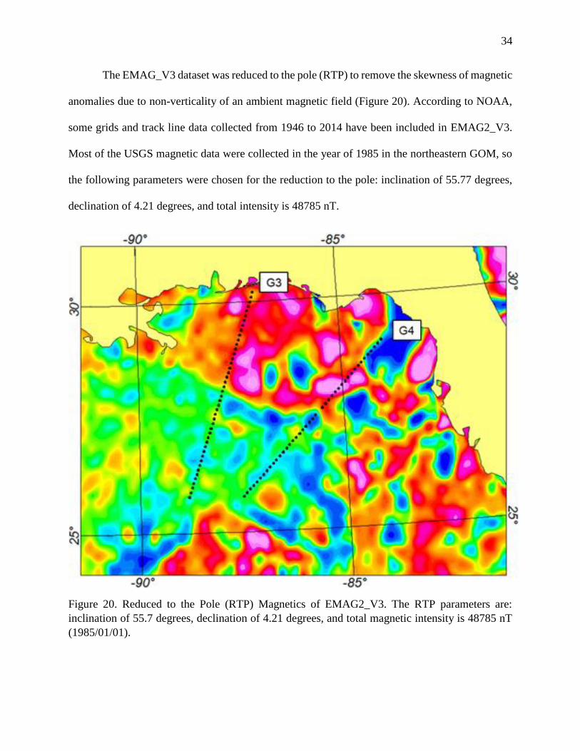
The EMAG_V3 dataset was reduced to the pole (RTP) to remove the skewness of magnetic
anomalies due to non-verticality of an ambient magnetic field (Figure 20). According to NOAA,
some grids and track line data collected from 1946 to 2014 have been included in EMAG2_V3.
Most of the USGS magnetic data were collected in the year of 1985 in the northeastern GOM, so
the following parameters were chosen for the reduction to the pole: inclination of 55.77 degrees,
declination of 4.21 degrees, and total intensity is 48785 nT.
Figure 20. Reduced to the Pole (RTP) Magnetics of EMAG2_V3. The RTP parameters are:
inclination of 55.7 degrees, declination of 4.21 degrees, and total magnetic intensity is 48785 nT
(1985/01/01).

35
2.5 Bathymetry
The bathymetry data used in this study are from British Oceanographic Data Center
(BODC)’s latest satellite data (Weatherall, 2015). The dataset has been gridded with a cell size of
1 km yielding a high resolution of bathymetric features in the basin (Figure 21). The bathymetry
data were used for calculating the Bouguer correction and for validating the locations for seismic
reflection profiles. Since the lines for modeling came from publications, the locations of the lines
were georeferenced from maps. To validate the location, the match between seismic seafloor and
real bathymetry was used. The good match in bathymetric features increases confidence in the
correct location of lines.
2.6 Earthquakes in the northeastern GoM
The earthquake parameters were downloaded from a USGS earthquake catalog
(https://earthquake.usgs.gov/earthquakes/search/). The locations of the earthquakes are plotted on
the bathymetric map (Figure 21). The earthquakes in the study area occurring in the period from
01/01/1800 to 05/06/2018 are listed in Table 4. The majority of the earthquakes in the northeastern
GoM have rather shallow focal depths, i.e. occurred within the sedimentary section. These shallow
earthquakes are caused either by sedimentary slumps (gravity driven slope failure), or by salt
tectonics. The magnitude of these shallow earthquakes is usually low. Although there are only
three deep crustal events (with the focal depth > 14 km) recorded in the USGS catalog, they were
more powerful than all earthquakes that occurred within the sedimentary section. Only two of
these deep events have focal mechanisms reported by the USGS. Both of them are located in the
oceanic region; their focal depth suggests the source in the crust or in the upper mantle. They both
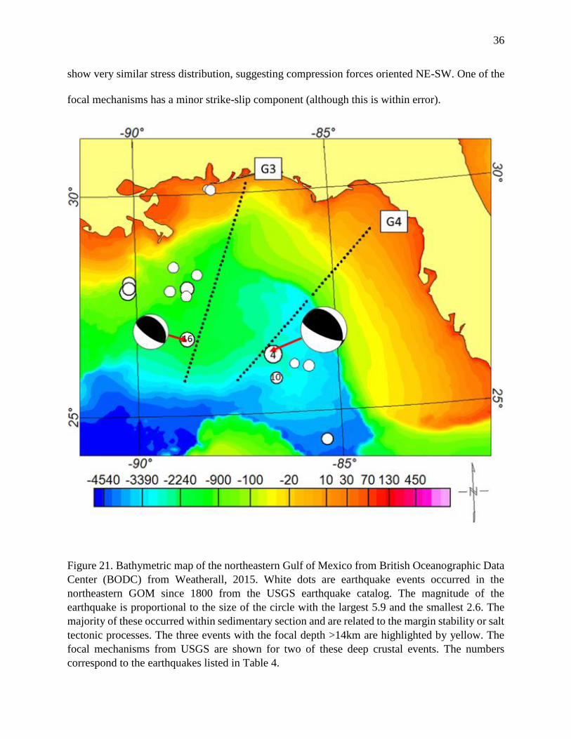
36
show very similar stress distribution, suggesting compression forces oriented NE-SW. One of the
focal mechanisms has a minor strike-slip component (although this is within error).
Figure 21. Bathymetric map of the northeastern Gulf of Mexico from British Oceanographic Data
Center (BODC) from Weatherall, 2015. White dots are earthquake events occurred in the
northeastern GOM since 1800 from the USGS earthquake catalog. The magnitude of the
earthquake is proportional to the size of the circle with the largest 5.9 and the smallest 2.6. The
majority of these occurred within sedimentary section and are related to the margin stability or salt
tectonic processes. The three events with the focal depth >14km are highlighted by yellow. The
focal mechanisms from USGS are shown for two of these deep crustal events. The numbers
correspond to the earthquakes listed in Table 4.

37
One of these crustal events is located next to GUMBO3 (Figure 21; earthquake 16 in Table 4);
it happened in 1978 and had a magnitude of 4.9. The depth of the earthquake was 33 km according
to the USGS earthquake catalog. The strike of the fault is aligned with the orientation of the ridge
segments (Figure 2b), however the earthquake is ~ 60 km to the north of interpreted extinct
spreading centers. USGS lists two possible nodal planes: one with a strike of 319°, dip of 26°, and
a rake of 102°, and another one with a strike of 126°, dip of 65°, and a rake of 84°. Another deep
earthquake with magnitude of 5.9 occurred in near the line GUMBO4 (Figure 21; earthquake 4 in
Table 4). This was the largest earthquake since 1800 in the eastern GoM. The location of
earthquake 4 is in Figure 21. The depth of the earthquake was 14 km. The strike of the fault is also
parallel to the ridge segments. The two suggested nodal planes are: strike of 324°, dip of 28°, and
a rake of 117° or strike of 114°, dip of 65°, and rake of 77°. One more crustal earthquake (number
10 in Table 4) occurred in 1997 at the depth of 33 km in the oceanic region of the northeastern
GoM. There is no information about focal mechanisms of this earthquake.

38
Tab
le 4
. E
arth
qu
akes
occ
urr
ing i
n t
he
stud
y a
rea
since
1800. T
he
eart
hqu
ake
dat
a ar
e fr
om
US
GS
ear
thquak
e ca
talo
g
(htt
ps:
//ea
rthquak
e.usg
s.gov/e
arth
quak
es/s
earc
h/)
. T
he
loca
tions
are
show
n i
n F
igu
re 2
1. T
he
eart
hquak
es w
ith t
he
foca
l dep
th >
14km
are
hig
hli
ghte
d.

39
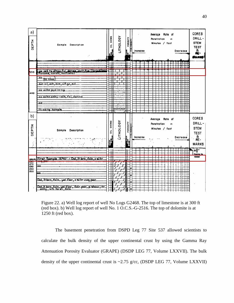
2.7 Well data
Well data were obtained from the Bureau of Ocean Energy Management website
(BOEM). Two well reports were used to constrain the depth to the top of the carbonate
platform along GUMBO3 profile and GUMBO4 profile. The locations of these two wells
are shown in Figure 10. Well No Logs G2468, which was operated by Gulf Oil Corporation
in 1975. The API number of the well is 608224001200. The top of the carbonate platform
is at a depth of 300 ft (Figure 22a). This well is close to GUMBO3 profile and was used to
constrain the model. Well No. 1 O.C.S.-G-2516, which was operated by Texaco Inc,
sampled the cores in 1975. The API number of this well is 608284000000. The top of the
carbonate platform is located at 1250 ft along GUMBO4 profile (Figure 22 b). According
to the biostratigraphy information provided in the well report, the top of the carbonate
platform is younger than upper Cretaceous.
40
Figure 22. a) Well log report of well No Logs G2468. The top of limestone is at 300 ft
(red box). b) Well log report of well No. 1 O.C.S.-G-2516. The top of dolomite is at
1250 ft (red box).
The basement penetration from DSPD Leg 77 Site 537 allowed scientists to
calculate the bulk density of the upper continental crust by using the Gamma Ray
Attenuation Porosity Evaluator (GRAPE) (DSDP LEG 77, Volume LXXVII). The bulk
density of the upper continental crust is ~2.75 g/cc, (DSDP LEG 77, Volume LXXVII)

41
which was used as the constraint for the two-dimensional subsurface modeling in the
following chapter.
The multiple velocity-density pairs from 447 deepwater wells in GoM from
Hiltermann et al. (1998) were used by Filina et al., (2015) to determine the general density-
velocity trend. Although the well data from Hilterman et al. (1998) were not explicitly used
in this study, the derived densities for individual sedimentary layers from Filina et al.
(2015) and Filina (2017) were utilized during the modeling of the gravity data.

42
CHAPTER 3. Integrated Geophysical Modelling
Three 2D subsurface models were built for this project along published seismic
profiles (Figure 7). The first model was aligned with seismic transect GUMBO3 (Eddy et
al., 2014). As the seismic reflection and refraction data for this line show some
disagreement in Moho interpretation (Figures 5 and 8), two versions of Model 1 were
developed. Model 1A followed seismic refraction data (Figure 5), and Model 1B was built
on seismic reflection data, suggesting shallower Moho (Figure 8). The second model was
aligned with line GUMBO4 from Christeson et al., 2014 (Figure 6). The third model was
developed along a seismic reflection line from Horn et al., 2017 (Figure 12).
Generally, the first step in the modeling is to split the subsurface into a number of
layers and then assign the physical properties (density and magnetic susceptibility) of each
layer based on additional constraints, such as well data or published values for various
types of rocks. The potential fields’ response was computed for each model and compared
with the observed signal. The model was then adjusted in order to ensure a good match
between observed and computed signals in both gravity and magnetic data. Thus, the
resultant model should remain geologically valid and agree with all available data –
seismic, gravity, magnetics and wells.
3.1 Models 1A and 1B
Profile GUMBO3 has a total length of 534 km. Both models 1A and 1B were
composed to a depth of 40 km (Figure 23), comprising 19 layers with various densities and

43
magnetic susceptibilities. The top ~10 km consists of seven sedimentary layers with their
modeled densities, respectively: Pleistocene (2.25 g/cc), Pliocene (2.35 g/cc), Miocene
(2.4 g/cc), Paleogene (2.45 g/cc), Mesozoic (2.55 g/cc), salt (2.15 g/cc), carbonates
(2.6 g/cc), and pre-salt (2.55 g/cc). The density values of sediments (excluding the pre-salt
deposits) were converted from velocity from 447 deepwater wells by Hiltermann et al.
(1998) and from Filina (2017). The multiple velocity-density pairs from 447 deepwater
wells in GoM from Hiltermann et al., 1998 were used by Filina et al. (2015) to determine
the general density-velocity trend. All sedimentary layers are assumed to be non-magnetic,
i.e., their magnetic susceptibility is 0 cgs. The profile from Rodriguez (2011) crosses
GUMBO3 (see Figure 10 for location). It was used to constrain the thickness of the
sediments in the first model. The seismic reflection data in the crossing point (Figure 13)
was converted from two-way travel time to depth by using the GUMBO3 seismic velocities
at the same point. The well G2468 (Figure 22) located 8 km away GUMBO3 was used to
constrain the top of the carbonate platform (91.44 m or 300 ft).
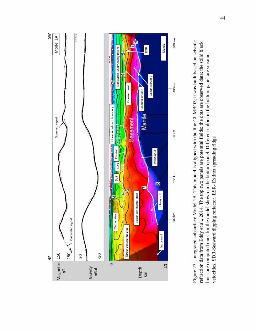
44
Fig
ure
23
. I
nte
gra
ted s
ubsu
rfac
e M
odel
1A
. T
his
model
is
alig
ned
wit
h t
he
line
GU
MB
O3;
it w
as b
uil
t bas
ed o
n s
eism
ic
refr
acti
on d
ata
from
Edd
y e
t al
., 2
014. T
he
top t
wo p
anel
s ar
e pote
nti
al f
ield
s: t
he
dots
are
obse
rved
dat
a; t
he
soli
d b
lack
lines
are
com
pute
d o
nes
for
the
model
show
n i
n t
he
bott
om
pan
el. D
iffe
rent
colo
rs i
n t
he
bott
om
pan
el a
re s
eism
ic
vel
oci
ties
. S
DR
-Sea
war
d d
ippin
g r
efle
ctor.
ES
R-
Exti
nct
spre
adin
g r
idge

45
The crust along this profile changes from a barely stretched continental one in the
beginning of the line to a much thinner oceanic one at the end of the line. The bottom layer
of the model is mantle with a density of 3.3 g/cc and 0 cgs magnetic susceptibility (Filina,
2017). In a continental domain, the crust is composed of two layers – the upper and the
lower continental crust units. The upper continental crust is ~6-~13 km thick. This layer
has a density of 2.75 g/cc constrained by the only basement penetration in the Gulf of
Mexico (DSDP LEG 77, Volume LXXVII) and magnetic susceptibility of 0.003 cgs
(converted from Filina, 2017). The SDRs are modeled in the upper continental crust with
a density of 2.75 g/cc and magnetic susceptibility of 0.005 cgs. The SDRs has a horizontal
extent of 20 km from Eddy et al. (2014) and a depth of 3 km in the upper continental crust.
The pre-salt sedimentary basin is bounded by SDRs in the north and by the OCB in south.
The density of a pre-salt section is assumed to be 2.55 g/cc and magnetic susceptibility is
assumed as 0 cgs. The crustal necking zone – the region in the continental domain where
crustal thickness changes from ~17 km to ~10 km - is located from 200 to 310 km along
the model.
The lower continental crust has not been drilled and was assumed to have a higher
density of 2.9 g/cc (Carlson and Herrick, 1990) and a higher magnetic susceptibility of
0.008 cgs. The magnetic susceptibility is determined during the modeling, but this value is
generally consistent with the range (6.9 +/- 2.0*10-3 cgs) published for the rocks of the
lower continental crust (Schnetzler, 1985). The OCB is interpreted at the distance of 310
km, which is coincident with a prominent magnetic signature. The location of the OCB is
very sensitive to the magnetic signal, so there is not much room to adjust the location for
the OCB. The model suggests the presence of three anomalous bodies (intrusions 1 - 3) in

46
the lower continental crust that span approximately between the following distances: 0 -
29 km, 87 - 140 km and 219 - 310 km. The intrusive bodies are modeled with a density of
2.95 g/cc and magnetic susceptibility of +/-0.01 cgs. The presence of intrusive bodies is
dictated by the magnetic signal. Potential field modeling does not have a unique solution.
The signal calculated for a subsurface model depends on geometries and physical
properties of the rocks in the subsurface. Thus, the depths of these intrusive bodies cannot
be uniquely determined by magnetic data alone. However, several zones of fast seismic
velocities (~7.5 km/s) are mapped in the refraction experiment (Figure5). Intrusion 2 and
3 are coincident with those fast Vp zones, which make them consistent with intrusive
bodies – highly magnetic and fast Vp. Intrusion 1 is not covered by seismic data (shaded
zone in Fiugre5), so it is the least constrained part on Model 1A, but its presence is
suggested by magnetic signal. The first two intrusions require reverse magnetic
susceptibility in order to match the observed magnetic signature.
Toward the center of the basin, oceanic crust was modeled from 310 to ~420 km
along the line. Since the seismic data for this line show some disagreement in the crustal
thickness (see Seismic Reflection Data section), two models were developed for the line
GUMBO3. The first model, shown in Figure 23 includes the oceanic crust composed of
two layers based on seismic velocities (basaltic upper layer with Vp varying from 6 to
6.5 km/s and lower oceanic crustal layer composed of gabbro with velocities of 6.5-
7.5 km/s). However, this crust appears to be thicker than normal from seismic refraction
data. The density of upper oceanic crust is 2.65 g/cc (Carlson and Herrick, 1990) and
magnetic susceptibility is assumed to be 0.007 cgs, which is consistent with the magnetic
susceptibility of basalt (Clark and Emerson, 1991). The density of lower oceanic crust was

47
2.95 g/cc (Carlson and Herrick, 1990) and the derived magnetic susceptibility was
0.008 cgs, which agrees with the magnetic susceptibility of gabbro (Clark and Emerson,
1991). The extinct spreading center, which is observed as a seismic velocity decrease in
the GUMBO3 profile (Figure 5), was also composed of two layers with the same density
as oceanic crustal units, but the magnetic susceptibilities of 0.006 cgs and 0.0009 cgs for
the upper and lower ridge respectively. These values were derived from magnetic modeling
and are within the published range of Schnetzler (1985).
For the alternative model - Model 1B shown in Figure 24 - the seismic reflection
data (Figure 8) were used as a constraint. The difference from the previous model is in the
oceanic domain adjacent to the OCB. In the previous model, the oceanic crust was 10 km
thick based on refraction data (Figure 5). In the seismic reflection data for the same line,
the oceanic crust near the OCB appears to be 4 km thinner. In the alternative model, this
crust was modeled as one layer with density 2.85 g/cc and magnetic susceptibility of
0.0075 cgs. These values were used to model a thinner oceanic crust for the adjacent
Model 2.
48
Fig
ure
24
. In
tegra
ted
subsu
rfac
e M
odel
1B
(t
he
loca
tion
coin
cides
w
ith
Model
1A
).
This
m
odel
is
bas
ed
on
Moho
inte
rpre
tati
on f
rom
sei
smic
ref
lect
ion l
ine
Fu
gro
53
3. T
he
Moh
o f
rom
pre
vio
us
model
(F
igure
23
) is
show
n a
s a
bla
ck l
ine.
To
sati
sfy t
he
obse
rved
pote
nti
al f
ield
s si
gnal
s, t
he
thic
knes
s of
the
upper
conti
nen
tal
crust
was
adju
sted
(se
e te
xt
for
det
ails
).

49
As already stated above, potential fields modeling does not yield a unique solution
for the subsurface structures as it responds to a combination of geometry (thicknesses and
geometric shapes of modeled layers) and physical properties (densities and magnetic
susceptibilities). That is why every potential fields model requires some constraints to
either geometries (from seismic data) and/or physical properties (from wells or from
published values for different types of rocks, such as in Telford et al. (1990). Model 1B
along Fugro533 (Figure 24) shares the same location as Model 1A and GUMBO3. It also
comprises 20 different layers. Most of the structures and physical properties of the
subsurface rocks are the same as in the previous model with the exception of the Moho
interpretation near the OCB, which is imaged shallower in seismic reflection data (Figure
8) than in seismic refraction data (Figure 5). In order to accommodate the misfits in the
gravity and magnetic signals generated due to changes in the crustal thickness and
properties, the boundary between the upper continental crust and the lower continental
crust has been adjusted geometry slightly in Model 1B. The mid-crustal boundary is the
least constrained one, while the basement and Moho are constrained by seismic refraction
database (Ibrahim et al., 1981). Both Model 1A and 1B are geologically valid with the
same physical properties, so no conclusion can yet be drawn as to which model is more
realistic at this stage. The density value of upper continental crust was adjusted to 2.77 g/cc
and of lower continental crust was adjusted to 2.95 g/cc in order to compensate the gravity
mismatch.
50
3.2 Model 2
Model 2 is aligned with GUMBO4 (Figure 6). This model has a total length of
510 km and thickness of 40 km (Figure 25). It comprises 17 layers with various densities
and magnetic susceptibilities. Compared to GUMBO3, the model along GUMBO 4 does
not have salt and SDR layers. The physical properties of all layers are the same as Fugro
533. Similar to GUMBO3, GUMBO4 has ~10 km thick sediments. The thickness of
siliciclastic sedimentary layer was modeled the same as GUMBO3. The top of the
carbonate platform at 381 m (1250 ft) was constrained from the well No. 1 O.C.S.-G-2516
(Figure 22). The necking zone along the line GUMBO4 is located from ~196 km to 295 km,
and shorter than the one observed for GUMBO3.

51
Fig
ure
25. M
odel
2 a
lign
ed w
ith p
rofi
le G
UM
BO
4 f
rom
Chri
stes
on e
t al
., 2
014. R
efer
to
Fig
ure
23
fo
r d
escr
ipti
on
.

52
The OCB is located at 295 km. The oceanic crust close to OCB has been modeled
as a single layer with a density of 2.85 g/cc and magnetic susceptibility of 0.0075 cgs. The
one-layer structure is suggested by the distribution of seismic Vp velocities (Figure 6).
Since the oceanic crust near the OCB does not show significant variations in Vp (7.0 km/s),
only one layer of oceanic crust was used for the segment extending from 295 km to 399 km.
From 399 km to the end of the profile, the oceanic crust has been modeled with two layers
as guided by seismic refraction data. The physical properties of all subsurface rocks are the
same as used for Models 1B. The extinct spreading center corresponds to the velocity
decrease from 460 km-497 km. The extinct spreading ridge (ESR) is located at the end of
the profile, which is consistent with Model 1A and 1B. An additional ESR1 structure was
added in the center of the one-layer segment of the oceanic crust in order to match the
observation from spatial analysis that will be discussed in Chapters 4 and 5. This additional
ridge structure is located roughly in the center of the one-layered oceanic crust and is 5 km
wide, too narrow to be detected from seismic refraction (the distance between the
instruments was 12 km in GUMBO4).
Several intrusive bodies in the lower crust were included in the model, similarly to
the ones shown in models 1A and 1B. However, some of them are slightly different from
those in GUMBO3. The first intrusive body is located in the continental domain at
distances of 73 to 192 km. Unlike GUMBO3, the seismic refraction data along GUMBO4
shows the velocity structure at the mid-crustal boundary is somewhat rugose, so the
intrusive body 1 was placed between the upper and the lower continental crustal units based
on the seismic refraction profile (Figure 6). The intrusion 2 starts at 73 km and ends at
241 km. The intrusion 3 was added based on the magnetic signal from 279 km to 295 km.

53
3.3 Model 3
Model 3 is located along Horn et al.’s (2017) profile (Figure 26). It has a length of
1071 km, extending from offshore Florida to the Yucatan margin (Figure 10). Model 3
consists of 19 layers up to depth of 36 km. The subsurface rocks were assigned the same
physical properties as all four models (Table 5). At this line crosses GUMBO3, the
thicknesses of individual subsurface layers were tied with GUMBO3 at the crossing point.
The thickness of continental crust at the beginning of the line is restricted by GUMBO4
since the lines are only 47 km apart. In addition, the pre-salt deposits and several salt
bodies were included in the model guided by seismic reflection images (Figure 12).

54
Fig
ure
26.
Inte
gra
ted s
ub
surf
ace
model
3. T
his
model
is
alig
ned
wit
h a
pro
file
fro
m H
orn
et
al. (2
017).
The
ph
ysi
cal
pro
per
ties
of
model
ed l
ayer
s ar
e li
sted
in T
able
5.
ES
R-
Ex
tinct
spre
adin
g r
idge.
S
DR
-Sea
war
d d
ippin
g r
efle
ctor.

55
Model 3 crosses two OCBs. The first one is located in the northeastern GoM at
~346 km, which corresponds to a magnetic trough. The second OCB is located in the
Mexican sector approximately 796 km along the line, which also is aligned with a trough
in the magnetic signal. The pre-salt deposits are imaged on the stretched continental
margins on both sides of the profile. The rifting necking zone in the northern part of this
model (248 - 346 km) is comparable to GUMBO4 but shorter than GUMBO3. The
continental crust on both sides of the line was modeled with two layers, i.e. the upper and
lower continental crustal units with the same physical properties as in the other models
(Table 5). Two intrusions were added to the continental crust in the northeastern GoM at
the following distances: 107-246 km (intrusion 1) and 270-322 km (intrusion 2). Both of
the intrusions are located in the lower continental crust in order to fit the gravity and
magnetic signal. Intrusion 1 has a reverse magnetic polarity and is modeled with a magnetic
susceptibility of -0.01 cgs, which is consistent with Model 1A, 1B. Intrusion 2 has a
positive magnetic polarity and is modeled with a magnetic susceptibility of 0.01 cgs, which
is also consistent with Model 1A, 1B, and 2.
As Model 3 is located in the region between GUMBO3 and GUMBO4 lines, it
allows study of the transition zone(s) between two distinct crustal domains imaged by those
profiles. GUMBO3 (Figures 5 and 8) shows generally thicker oceanic crust (9 km thick),
while the oceanic crust along GUMBO4 is dramatically thinner (~5 km) and shows a
different velocity profile (Figure 6). Model 3 (Figure 25) shows three distinct crustal zones
in the oceanic domain. The first zone spans from the OCB in the northeastern part of the
line (346 km) to 447 km; it is consistent with one-layered (gabbroic) thinner crust, similar

56
to the one imaged with Model 2 (GUMBO4) with a density and magnetic susceptibility of
2.85 g/cc and 0.0075 cgs. The extinct spreading ridge in the center of the one-layer crust
(ESR1) was modeled with a density and magnetic susceptibility of 2.85 g/cc and 0.009 cgs.
This distinct feature was observed as gravity low in spatial analysis (See Chapter 4), so it
was added to be consistent with spatial analysis. Further, between 440 km and 638 km, the
crust is consistent with thicker two-layered (basaltic and gabbroic) one, imaged by Models
1A and 1B (GUMBO3) with densities 2.65 g/cc and 2.95 g/cc respectively, and
corresponding magnetic susceptibilities of 0.007 cgs and 0.008 cgs. From 638 km to 796
km (the OCB on the Yucatan side), the oceanic crust was modeled with single gabbroic
layer again. The ESR was determined in a middle of a two-layered segment between 544
km and 612 km in order to match magnetic signal. The changes in the oceanic crustal
structure observed along this line are consistent with the overall variations of oceanic crust
observed for GUMBO3 and GUMBO4 and will be addressed in detail in the Discussion
section below. Notably, the sharp bump at the model distance of 618-638 km has a
magnetic signal that is an artifact in the public magnetic datasets. This bump was not
observed in Pindell et al. (2016)’s regional aeromagnetic data.
From the three models described above, the density and magnetic susceptibility of
subsurface rocks have been derived. They are listed in Table 5. The physical properties of
the corresponding layers that are derived from these four models (Model 1A and 1B, 2, 3)
are either constrained by the well data (sedimentary layers and upper continental crust) or
with published values. The intrusions in the necking zone have consistent positive magnetic
susceptibility. The OCB is located at model distance of 310 km in Model 1A and 1B, at
model distance of 295 km in Model 2, and at model distance of 346 km in Model 3. The

57
derived OCB locations from the four models correspond to magnetic troughs with
uncertainty within 7 km. The ~3 km thick pre-salt section from Model 1A and 1B is
modeled in order to match the magnetic signal, but is not observed from seismic refraction
data (Figure 5), nor can be confidently identified in the seismic reflection data (Figure 8).
There is no pre-salt section in the Model 2 (GUMBO4) and it is only 1 km thick in Model
3. Several intrusions of various magnetic polarity (positive or negative) were modeled
primarily based on the characteristics of Vp from refractions and based on magnetic
anomalies. The depths of major modeled horizons are consistent between all the models as
listed in Table 6.

58
Table 5. Physical properties of the subsurface layers for all three models.
Layer in the model Density (g/cc) Magnetic susceptibility
(cgs)
Pleistocene 2.25 0
Pliocene 2.35 0
Miocene 2.4 0
Paleocene 2.45 0
Mesozoic (including the pre-
salt sediments) 2.55 0
Carbonates 2.6 0
Salt 2.15 0
SDR 2.75 0.005
Upper continental crust 2.75
2.77 for Model 1B 0.003
Lower continental crust 2.9
2.95 for Model 1B 0.008
Intrusions1 and 2 in Models
1A and 1B
Intrusion 1 in Model 3
2.9 -0.01
Intrusion 3 in Models 1A
and 1B
Intrusion 2 and 3 in Model2
2.9 0.01
Intrusion 1 in Model 2 2.75 (upper crust) 0.01
Oceanic crust layer 2 2.65 0.007
Oceanic crust layer 3 2.85 0.008
One layered oceanic crust 2.85 0.0075
ESR (upper layer) 2.65 0.006
ESR (lower layer) 2.95 0.009
ESR1 in one-layered crust 2.85 0.009
Mantle 3.3 0

59
Table 6. The depth to major layers boundaries in km measured at the beginning and the
end of the modeled profiles.
Depth at the beginning of the line,
km Depth at the end of the line, km
Models 1A
and 1B,
GUMBO3
Model 2,
GUMBO4
Model
3,
Horn et
al., 2017
Models
1A and
1B,
GUMBO3
Model 2,
GUMBO4
Model
3,
Horn et
al., 2017
Top of
carbonate 2.07 1.42 2.88 N/A N/A N/A
Top of
basement 7.61 4.98 4.95 9.9 10.15 9.38
Mid-crust
boundary 19.42 19.27 19.25 11.79 12.15 12.34
Moho 33.33 33.35 35.05 19.46 15.52 17.09

60
Chapter 4. Spatial Analysis of Gravity and Magnetic Fields
4.1 Filtering of potential fields
Potential fields (gravity and magnetics) are sensitive to lateral variations in physical
properties of the rocks in the subsurface. Different rocks have different densities and
magnetic susceptibilities (Telford, 1990). Major geological boundaries represent the
contacts between the rocks of different type (OCB, SDR, basement faults). These contacts
are associated with some signals in the potential fields and these signals may be different
amplitude and wavelength depending on the magnitude of the contrast in physical property,
geometry, and depth of the contact between juxtaposed rocks. Hence, the recorded potential
fields represent the superposition of all the signals due to various geological structures in
the subsurface. In order to highlight the specific one that this study focused on, which is
the crustal layer structures, the other signals need to be removed. A series of corrections
were made to take into account the known sources of potential fields’ signals, such as the
Bouguer correction in gravity and reduction to the pole in magnetics. The effects of deeper
sources (Moho and below) could also be removed by estimating and subtracting the
regional trend from the observed potential field. Further, a series of filters (mathematical
transformations) may be applied to highlight the crustal signatures that focus on the regions
where the fields change the most.
The gravity effect of water contacting with unconsolidated sediments of the
seafloor was calculated and removed from the observed Free-Air gravity anomaly (see
Geophysical Data section for details). The resultant Bouguer gravity anomaly is shown in
Figure 18. The regional gravity trend, representing the signal from the deep sources (Moho

61
and below), was computed via application of the upward continuation filter to the Bouguer
gravity anomaly to the level of 40 km and then removed from the Bouguer gravity
anomaly. The resultant residual Bouguer gravity anomaly is shown in Figure 27. It
represents the gravity effects for all sources between the mudline and Moho, such as salt
in the sedimentary cover and variations within the basement. As the salt is generally much
shallower in the section, its signature is usually manifested by short-wavelength anomalies,
while the basement and the rocks variations within the crust are usually associated with
wider anomalies.
Figure 27. (a) Residual Bouguer Gravity of the northeastern Gulf of Mexico calculated for
the satellite gravity data (Sandwell et al., 2014). This gravity anomaly represents the signal
for all the sources between the mudline and the Moho. (b) Residual magnetic anomaly
computed for the EMAG2_V3 dataset (Meyer et al., 2017). These magnetic anomalies
represent the variations in magnetic susceptibilities within the crustal rocks (the sediments
were assumed to be non-magnetic as their magnetic susceptibilities are several orders of
magnitude lower than the igneous and metamorphic rocks).
In magnetic data, reduction to the pole was applied to un-skew the observed
anomalies (see Geophysical Data section for details). The regional trend was calculated by
applying an upward continuation filter with an elevation of 20 km as the magnetic field

62
decays much faster than the gravity field. The resultant residual magnetic anomaly is
shown in Figure 27b.
Before intepreting the geological structures in the residual potential fields, a
number of different filters were applied to test which one highlights them better: the first
vertical derivative filter, various low and high pass filters, and the tilt derivative filter
(Blakey et al., 2016). A tilt derivative of the residual Bouguer gravity map (Figure 28a)
shows the lineaments better than the other tested filters; therefore, most of interpretations
were based on tilt derivative transformation of the residual Bouguer gravity map. This map
(Figure 28a) shows a strong pronounced high that surrounds a series of gravity lows in the
center of the basin.
Figure 28. a) Tilt derivative of residual Bouguer gravity. b) First vertical derivative of the
residual RTP magnetic map.
In magnetic data, the first derivative filter (Figure 28 b) highlights the structures
better than the tilt derivative filter. The first vertical derivative of the residual RTP
magnetic map shows a series of prominent magnetic highs in the center of the oceanic
region that are surrounded by magnetic lows. In general, the magnetic anomalies appear to

63
be less pronounced than the gravity ones. However, some of magnetic high in the center of
the basin correlate with gravity lows (Figure 28 a), while the surrounding magnetic lows
generally coincide with the pronounced gravity high. As the anomalies are better
highlighted in the filtered gravity field than in magnetic data, the spatial analysis was
guided by a filtered gravity map.
4.2 Correlation with 2D subsurface models
As has been stated above, the tilt derivative of residual Bouguer gravity and the
first vertical derivative of RTP magnetics show the clearest lineaments (Figure 28 a, b).
The correlation of the observed lineaments with the geological structures interpreted from
the three modeled profiles is illustrated in Figure 30.

64
Fig
ure
29
. a)
Til
t der
ivat
ive
filt
ered
map
of
resi
du
al B
ou
guer
Ggra
vit
y f
ield
. b)
Ver
tica
l der
ivat
ive
filt
ered
map
of
RT
P
mag
net
ics.
Lin
eam
ents
are
lab
eled
in t
he
map
s. B
lue
line
den
ote
s th
e lo
cati
on o
f S
DR
. O
ran
ge
line
den
ote
s pre
-sal
t
loca
tion. P
urp
le l
ine
den
ote
s th
e lo
cati
on o
f O
CB
. D
ark g
reen
lin
e den
ote
s th
e lo
cati
on o
f youn
g r
idge.
Yel
low
den
ote
s th
e
loca
tion o
f fo
ssil
rid
ge

65
The location of the OCB from the three models, i.e. ~310 km along Models 1A and
1B (GUMBO3), ~295 km along Model 2 (GUMBO4) and ~346 km along Model 3
(between Models 1 and 2) were marked on the tilt derivative of residual Bouguer gravity
and vertical derivative RTP magnetic maps as purple lines (Figure 30). The OCB locations
for all three models correspond to the same gradient in the filtered gravity (edge of a
pronounced high). In magnetic data, they are consistent with linear magnetic low.
Interpreted extinct spreading centers are marked with bright yellow on the maps in
Figure 29. The larger ones, correlating to gravity lows, are outlined by dark green color.
The edge of the pre-salt basin from models 1 and 3 are also marked on both maps with
orange color. These correlate with lows in both gravity and magnetics. The pre-salt section
extends all the way to the edge of the continental domain marked by an OCB. The SDR
province is marked with blue color along Models 1 and 3 as well as Model 2 (GUMBO4)
does not cross either a pre-salt basin or the SDR region. All the locations from 2D
subsurface models are described in the previous chapter.
4.3. Combined Interpretations of the Tectonic Structures in the Study Area
The correlation between the lineaments and interpreted geological structures
allowed extension the interpretations to areas outside of seismic coverage by tracing along
the gradients and lineaments in the filtered potential fields. Figure 30 shows the ocean-
continent boundary, the extinct spreading centers and the extent of the pre-salt deposits
mapped in the study area

66
Fig
ure
30
. M
apped
geo
logic
al s
truct
ure
s in
the
NE
GoM
on f
ilte
red g
ravit
y a
nd m
agnet
ic m
aps.
a)
Til
t der
ivat
ive
of
resi
dual
Bouguer
gra
vit
y m
ap. b)
Ver
tica
l der
ivat
ive
of
RT
P m
agnet
ic m
ap. B
row
n c
ircl
es d
enote
ES
R. T
he
whit
e ci
rcle
s d
enote
foss
il
ridges
. G
rey l
ine
is t
he
OC
B. P
ink p
oly
gon o
utl
ines
the
pre
-sal
t bas
in. B
lue
das
h l
ine
indic
ates
SD
R

67
The OCB is characterized as a gravity high and magnetic low. A Gravity low and
magnetic high refer to all segments of the fossil spreading center in the northeastern GoM.
The northern edge of the SDR province corresponds to gravity low and magnetic low, while
the pre-salt basin is marked by gravity low and magnetic high. The pre-salt basin wedges
out to the east (as confirmed by model 2 (GUMBO4) and is bounded by an SDR province
in the north and by the OCB in the south.
The pre-salt sedimentary basin is 64 km wide along Models 1A and 1B (GUMBO3)
with a thickness of 3 km. The thickness is consistent with FloridaSPAN profile that images
3-4 km thick pre-salt section (Figure 15). There is only a minor amount of pre-salt basin
along Model 3, with a lateral extent of 9 km and a depth of 1 km. No pre-salt was found
along Model 2 (GUMBO4). Therefore, the pre-salt section wedges out to the east
(Figure 30).
4.4 Validation of interpreted geological structures with the literature
Interpretations from this study have integrated seismic refraction, seismic
reflection, gravity, and magnetic data compared to previous analyses. The interpreted
geological structures were validated with several published seismic datasets, including the
OCBs published by Bird et al. (2005); Hudec et al. (2013); Sandwell et al. (2014); Pindell
and Keenan (2009); Christeson et al. (2014); Nguyen and Mann (2016) (Figure 31), the
depth to basement map from 3D survey from Deighton et al. (2016) (Figure 33), and several
seismic reflection profiles from Snedden et al. (2014), FloridaSPAN (2015), and Saunders
et al. (2016) (Figure 33).

68
Figure 21 a shows defined OCBs from different studies. The OCB from this study
is most close to Sandwell et al. (2014) with minor offset in the eastern side of GUMBO4
profile and southern GoM. Pindell and Keenan (2009) and Nguyen and Mann (2016)
placed the OCB further north. Bird et al. (2005) placed the OCB closer to the center of the
basin. Hudec et al. (2013) has a similar interpretation of the OCB where it is close to the
GUMBO profiles but wider than the rest of the OCB from this study. The OCBs derived
from those studies were based on only seismic interpretation or gravity method, while this
study integrates both potential fields and seismic to constrain the location of the OCB.
Figure 31. Comparison of different published OCBs with interpretation from this study.
Three red lines are the integrated subsurface models developed in this study. The
background is vertical gravity gradient from Sandwell et al., 2014.
The comparison between this study’s interpreted extinct mid-ocean ridge segments
generally agree with the interpretations of Sandwell et al. (2014). However, instead of three
continuous spreading centers in the northeastern GoM, this study has interpreted the
69
spreading centers as short isolated segments from spatial analysis (Figure 32). Nguyen and
Mann (2016) interpreted the spreading centers slightly offset to the south (Figure 32).
Figure 32. Comparison of different published spreading centers (Sandwell et al., 2014 and
Nguyen and Mann, 2016) with this study’s interpretation. The purple line is axial valley
along interpreted ridge from this study.
The results of the recent 3D seismic reflection survey (Deighton et al., 2017) agrees
very well with the interpretation herein of extinct spreading centers (Figure 33). The
location of the 3D seismic survey is outlined in Figure 10. The background of this Figure
14 is depth to basement map from 3D seismic reflection survey. The ridges and transform
faults from Deighton et al. (2017) are shown in red. The brown color is the interpretation
of spreading centers from this study. The interpreted spreading centers show good
correlation with mid-ocean valleys. From this 3D survey, at least three segments of mid-
ocean valleys were validated as well as three transform faults (Figure 33).

70
Figure 33. Comparison between TGS’s map (Deighton et al., 2016) of extinct spreading
centers with the ones interpreted in this study from integrated analysis of various
geophysical datasets.
The interpreted SDR province is ~54 km wide and 335 km long. It is ~ 59 km longer
that the one outlined by Eddy et al (2014). The NW edge of the Eddy at al. (2014) SDR
province is coincident with GUMBO3 and appears to be limited by availability of seismic
data. The interpretation from this study is based on the signals in filtered potential fields
data (Figure 30) and the constraints from Models 1 and 3 (Figure 29). Moreover, a similar
SDR province is imaged by multiple seismic reflection profiles in the southern GOM
(Williams-Rojas et al., 2011, Saunders et al., 2017; O’Reily et al., 2017, Horn et al., 2017).

71
Similar integrated geophysical analysis performed in the southern GoM by Hartford and
Filina (2018) outlined an SDR province that is 55 km wide and 360 km long. To be
consistent with the interpretation on the conjugate margin, the SDR province in the study
area was extended to NW of Eddy et al.’s (2014) outline.
The profile from Snedden et al. (2014) crosses the extinct spreading center. The
extent of the gravity low is shown as a horizontal bar on top of the seismic image in
Figure 16, thus validating the interpretation that the extinct spreading ridges are
characterized as gravity lows. This profile also crosses the OCB and the pre-salt basin that
are also marked in Figure 16.
Another seismic reflection profile – the one from Saunders et al. (2016), shown in
Figure 11 - can be used to validate interpreted extinct spreading centers. This profile
partially overlaps the line GUMBO3. The ‘valley’ feature (black box in Figure 11)
corresponds to pronounced gravity low and magnetic high that are interpreted as an extinct
spreading center.

72
CHAPTER 5 Discussion
5.1 Observations from this study
As a result of the potential fields modeling along three seismic lines, the densities
and magnetic susceptibilities of the subsurface rocks were determined (Table 5) and the
location of the key tectonic structures were constrained (Figure 30). The joint spatial
analysis of gravity and magnetic fields, calibrated with three subsurface models, allowed
us to determine the lateral extent and the thickness of the pre-salt sedimentary section, as
well as to characterize the crustal architecture. The location of the OCB, correlated to a
gravity high and magnetic low, was also determined from the integrative analysis of
potential fields.
The width of the necking zone in the continental domain decreases toward to the
east in the study area from 110 km for Models 1A and 1B to 99 km for Model 2 and 98 km
for Model 3. The width of the necking zone may be considered as an additional constrain
for tectonic reconstruction, as it should match on both margins assuming symmetric
continental rifting.
The extinct spreading centers are clearly mapped in gravity data as pronounced
gravity lows. The locations of the spreading centers were confirmed by seismic data
(Figures 11, 14 and 16) and generally agreed with published interpretations (Sandwell et
al., 2014; Figures 32 and 33). However, several new spreading centers were identified in
the Models 2 and 3 (Figures 25 and 26). These new identified features are observed as
small gravity lows and magnetic highs. For example, the new spreading center identified
along Model 3 at distance 394 km (Figure 26) correlates to a small gravity low (Figure

73
30a) and magnetic high (Figure 30b). The presence of these newly identified spreading
centers lead to a hypothesis about ridge propagation in the northeastern GoM – the jump
of the spreading center from the old location (small newly identified features in the
northern part of the oceanic domain) to the south, where the more pronounced (younger)
spreading center is mapped. The older spreading center in the north produced thinner one-
layer crust, while the younger one in the south is associated with thicker, two-layered
oceanic crust. This hypothesis about ridge propagation, suggesting two spreading centers
in the history of the GoM, is also consistent with the observed asymmetry in seafloor
spreading that was noted by some authors (Hudec et al., 2013; Nguyen and Mann, 2016).
5.2 The ridge jump in literature
Ridge jump in the East Pacific Rise (EPR) is clearly seen in bathymetry data (Figure
34). The East Pacific Rise is a fast-spreading ridge with spreading rate of 7-8 centimeter
per year (Rea, 1977). This fast spreading rate agrees well with the overall ridge morphology
represented as axial highs (Carbontte et al., 2000). The jump of the spreading center to the
west led to the formation of a microplate in between the East Pacific Rise and the
Galapagos Rise. The Galapagos Rise (fossil ridge) started spreading about 17-15 Ma
(Eakins and Lonsdale, 2004). Early ridge propagation to the west occurred in 15 Ma
(Eakins and Lonsdale, 2004). In Miocene (~8 Ma), the East Pacific Rise began actively
spreading (Rea, 1976).

74
Figure 34. a) The East Pacific Rise from a global view of GoogleEarth. b) The bathymetry
map of the East Pacific Rise from GeoMapApp. The ridge propagation is clearly seen with
the older ridge segment on the east, and the younger one on the west.
In contrast, the GoM is believed to be a slow spreading system with an estimated
spreading rate of 2.2 centimeters per year (Christeson et al., 2014). As there is an obvious
difference in the spreading rates between GoM and EPR, the fast spreading EPR cannot be
considered as a proper analog for the slow-spreading GOM. However, due to pronounced

75
structural ridges, the EPR bathymetry shows the overall geometry and organization of the
propagation ridge very clearly, so it has been used in this study to illustrate the concept.
The crust in the center of the GoM is covered with over 8 km thick layer of
sediments, so bathymetry data does not show the spreading centers, moreover any ridge
propagation structures. Thus, the filtered gravity data were used to map the extinct
spreading centers (Figure 28a). In order to test the hypotheses that gravity data may be used
to map the ridge propagation, the gravity data over the East Pacific Rise were also filtered.
The same mathematic transformations were applied to the Free-Air gravity over the East
Pacific Rise, downloaded from Sandwell et al. (2014), with two exceptions. The upward
continuation to an elevation of 15 km was applied to compute the regional trend (in contrast
to 40 km for GOM) as the Moho is at a shallower depth over the EPR compared to the
GoM. Then the residual gravity field over the East Pacific Rise was additionally continued
upward to an elevation of 8 km to mimic the presence of the thick sedimentary layer in
order to compare with the GoM.
Filtered gravity map of the EPR was rotated 90 degrees (Figure 35a, b) with the
intention of having a better structural alignment with the features in the GoM (Figure 35c).
The resultant Figure 35b shows both old and young ridges over the EPR as noticeable
gravity lows. The young spreading segments appear to be larger and more pronounced than
the old ones. The filtered gravity over the GoM appears to have a similar pattern of gravity
anomalies, overall suggesting ridge reorganization.

76
Figure 35. a) Bathymetry of the EPR rotated 90 degree counterclockwise in order to better
illustrate the correlation of the propagating ridge segments with the ones in the GoM. b)
Tilt derivative of residual Bouguer of the East Pacific Rise also rotated 90 degrees. Brown
color outlines an active spreading ridge. White color outlines a fossil ridge. Green box
shows pseudofaults – the boundary between old and new oceanic crustal domains, c) Tilt
derivative of residual Bouguer of the GoM. Brown color indicates the younger spreading
ridge. White color outlines fossil ridge. Pseudofaults are marked as purple lines.

77
Migration of the spreading ridge creates a wake of pseudofaults that are oblique to
the ridge axis and point in the direction of offset migration (Kleinrock et al., 1997; Figure
36a). Pseudofaults form a V-shaped wake behind the propagating spreading ridge pointing
in the direction of propagation, marking previous locations of the propagator tip (Screejith
et al., 2016; Figure 36b). The V shape pseudofaults in the East Pacific Rise are observed
from the Google Earth image (outlined with a green box in Figure 36a). In the filtered
gravity map (Figure 35 b), the pseudofaults are characterized by gravity highs in the East
Pacific Rise. The pseudofaults are associated with a vertical trough in the basement
according to an integrative analysis of basement characteristics and gravity data from
Screejith et al., 2016.
Figure 36. a) V shape pseudofaults in the East Pacific Rise from Google Earth. This picture
has been rotated 90 degrees in order to corresponds to Figure 35 a. The pseudofaults are
outlined by green box. b) The mechanisms of forming the V shape pseudofault (modified
from Screejith et al., 2016). PR-Propagating Ridge. RR- Receding Ridge. TC-Transferred
Crust. IPF-Inner Pseudofault. OPF-Outer Pseudofault. FR- Failed Ridge.

78
5.3 Propagating ridge in the GoM
The subsurface models developed for this study (Figures 23, 24, 25 and 26) mapped
three locations that mark a change in the oceanic crustal structures, i.e. the location of
pseudofaults (Figure 35c). Two of the locations along Model 2 and 3 correlate to
pronounced gravity highs in the filtered gravity map. The one from Models 1A and 1B is
characterized as a gravity low. This is because the location of that pseduofault appears to
be overprinted with the transform fault mapped by Deighton et al. (2017) as troughs in the
basement (Figure 14). Furthermore, this location along GUMBO3 was checked with 2D
seismic reflection data, which suggests a valley (white box in Figure 11). This is consistent
with observation from Deighton et al. (2017) that transform faults and extinct spreading
centers are both characterized as axial valleys in the western GoM. Therefore, the
superposition of these two structures - pseudofault (the contact zone between two distinct
crustal domains) and the younger transform fault – complicates the interpretation of the
gravity anomaly. By analogy with the pseudofaults observed over the EPR (Figure 35b),
these three spots are interpreted to mark the pseudofault or a boundary between the old and
new oceanic crustal segments.

79
Figure 37. The location of a pseudofault in the northeastern GoM on the tilt derivative of
residual Bouguer gravity map. The 3D seismic data interpretation from Deighton et al.,
2017 is superimposed on the gravity map. The red transform fault close to GUMBO3
terminates at the pseudofault. The light purple marks show the points of contact between
two distinct crustal domains from three modeled profiles. These correlate to gravity highs.
The dark purple line shows the interpreted boundary between the old oceanic domain in
the north and the young one in the south. Brown outlines denote the young spreading
centers, while the white ones show the old spreading centers that identified from this study.
Grey line shows the OCB interpreted in this study. The bright blue lines in the continental
region overlap three models indicate the location of negatively polarized intrusion. The
green lines overlap three models in the continental region indicate the location of positively
polarized intrusion. The white dots are earthquakes from USGS Earthquake Catalog.
According to Reid and Jackson (1981), there is a positive correlation between
oceanic crustal thickness and spreading rate. Slow spreading results in a thinner oceanic
crust, while a fast-spreading forms the thicker crust. The example of the modern slow
80
spreading ridges is the Mid-Atlantic Ridge with the crust varying in thickness from 2 to
7 km at the Kane fracture zone (Chen, 1992). The fast-spreading systems result in a thicker
crust, like the East Pacific Rise (5-8 km from Chen, 1992). Therefore, the thinner oceanic
crust in the GoM (along the Model 2) appears to be produced by a slower spreading center
than the thicker one from Models 1A and 1B. The thin and dense oceanic crust with fast
seismic velocity (Vp ~7.0 km/s) and high magnetic susceptibility, presumably composed
of gabbro, is most likely produced by ultraslow spreading. This crust was interpreted
immediately to the south of the OCB in the Model 1B (Figure 24) and in the Model 2
(Figure 25); this segment was also modeled twice in the Model 3 (Figure 26) adjacent to
both continental domains. In contrast, the thicker, two-layered crust suggests a faster
spreading rate associated with a higher magma supply. However, the fact that the younger
extinct spreading centers are imaged in seismic reflection data as valleys, rather than ridges,
suggesting that the thicker, two-layered crust was still produced by a relatively slow
spreading ridge (Figures 11, 14 and 16).
According to Snedden et al. (2014), the age of the oceanic crust may be constrained
from the age of the oldest sediments overlying the crust tied to several onshore wells
(Figure 39). That study concluded that the oldest oceanic crust in the northeastern GoM is
155 -160 Ma old and that oceanic crust ceased before 137 Ma ago. The pseudofaults
location that derived from this study is align with the 150 Ma contour line in Figure 39.
Thus, by measuring the width of the oceanic segments on each side of the pseudofault and
using the age from Snedden et al. (2014), the spreading rate of each spreading event may
be estimated. The oceanic segment associated with fossil ridge is 96 km wide on average,
and the estimated spreading rate was 9 mm/yr (full spreading rate) by assuming the first

81
spreading episode lasted 10 Ma. The young crust zone is 146 km wide on average and the
estimated spreading rate was 1.1 mm/yr by assuming the second spreading episode lasted
13 Ma.
The initial spreading rate for the oldest segment is consistent with an ultra-slow
spreading. The younger spreading agrees with the slow spreading centers imaged in seismic
data as valleys (Saunders et al., 2016, Figures 11). The faster spreading rate for the younger
ridge with respect to the fossil ridge is consistent with the generally thicker crust and the
presence of basaltic layer on top of the oceanic layer 3 (gabbro).
Before 150 Ma when the ridge reorganization occurred and the young ridge started
spreading, the segments of the old ridge were aligned. Figure 38 shows the total extent of
the oceanic crust produced by the first seafloor spreading event in the GoM.
Figure 38. The distribution of old oceanic crust produced by a fossil ridge before the
young ridge started spreading. The thick purple line indicates the boundary between the
young crust and old oceanic crust in the northeastern GoM. The dashed purple line is
extrapolated by tracing similar gravity signals (highs). White circles indicate the old
extinct spreading centers.

82
Figure 39. Plate tectonic reconstruction for the eastern GoM modified from Snedden et al.,
2014. Different colors in the background indicate different ages of the crust. The solid
black lines in the center are the proposed spreading centers from Snedden et al., 2014. The
purple marks that overlap with age of 150 Ma indicate the boundary between old spreading
event (brown outlines) and young spreading event (white outlines). Grey line indicates the
OCB from this study.
This study infers that at 150 Ma (age from Snedden et al. 2014, Figure 39), a
presumable change in tectonic stresses occurred leading to a change in the Euler pole. This
resulted in a consequent ridge propagation to the south in the eastern GoM. At the same
time, the ridge propagated to the north in the central GoM (Figure 38). The oceanic crust
in the easternmost part was not spreading before 150 Ma (Figure 40). Thus, the easternmost
part of oceanic domain is characterized by a symmetrical spreading. In contrast, the oceanic
crust to the west appears asymmetric due to ridge propagation.

83
Figure 40. The formation of oceanic crust in the northeastern GoM. The crust in the center
of the study area shows the evidence of ridge propagation to the south, presumably at
150 Ma (Snedden et al., 2014). Brown circles are young extinct spreading centers. White
circles are fossil spreading centers. The crust in the easternmost part of the study area is
symmetric as it initiated after ridge propagation at 150 Ma.
The younger crustal segments are thicker and have basaltic layer on the top, which
was determined from the derived physical properties, namely Vp ranging from 5 to
6.5 km/s, and modeled density of 2.65 g/cc (Carlson and Herrick, 1990). This suggests an
increase in magma supply from older to younger spreading events.

84
The interpreted ridge jump in the GoM is consistent with the finding of Pindell et
al. (2016), who determined the change in the rotation pole between 152 and 145 Ma to the
southeast. Figure 41 shows the boundary between different crusts (early oceanic crust and
late oceanic crust) that was proposed by Pindell et al. (2016) aligns well with the
pseudofaults interpreted in this study.
Figure 41. Map of four primary basement types modified from Pindell et al. (2016) with a
pseudofault zone from this study superimposed (thick purple line). The green crust is
hyper-extended crust/exhumed mantle interpreted by Pindell et al. (2016). The yellow crust
is earlier oceanic crust (Oxfordian-Tithonian, 159-150 MA). The blue crust is later ocean
crust (Tithonian-Top Berriasian, 150-139 MA). White crust is rifted continental margins
in the GoM. See caption details in Figure 39. The red dot in the center is proposed pole1
from Pindell et al. (2016). The red dot at the bottom of the map is the proposed finite pole
for the Yucatán restored from today’s position to the Bathonian position from Pindell et al.
(2016). The green dashes line is the ocean-continent boundary from Pindell et al. (2016).
85
However, the OCB between this study and Pindell et al. (2016) shows some
dramatic discrepancies (Figure 41). The wider OCB from Pindell et al. (2016) resulted
from assumed rifting symmetry that is forced in the model shown in Figure 41. Moreover,
the exhumed mantle, suggested by Pindell et al. (2016), is not supported by this study.
According to Pindell et al., 2016 (Figure 41), the reconstruction of the basin lead to changes
of the Euler Pole three times. This study confirms at least one evidence of the change in
the location of the Euler pole that is related to the ridge propagation, presumably at 150 Ma,
that would relate to Pindell et al.’s jump from Pole 2 (159-150 Ma) to Pole 3 (150-139 Ma).
Furthermore, the pseudofault boundary derived in this study is aligned with the
locations of several crustal earthquakes (Figure 37) that were described in Chapter 2. The
earthquakes focal depth is over 14 km, suggesting they are lithospheric events. However,
they were not aligned with any known tectonic structures. According to this study, they
occurred in a zone of weakness between two distinct crustal domains due to two spreading
episodes. This zone appears to be reactivated with the current compressional stress
(identified from two identical focal mechanisms; Chapter 2). Therefore, the location of
pseudofault is confirmed with the observed seismicity in the study area.
This study concludes that the oceanic crust in the GoM formed in two stages.
The first spreading episode started ~155 to 160 Ma (Snedden et al., 2014) and resulted in
thin, dense, and highly magnetic oceanic crust with a uniform seismic velocity profile
(Vp ~7 km/s). The younger crust shows much thicker, two-layer structure (basaltic layer
overlays gabbroic layer) suggesting an increase in the supply of magmatic material.
Two models were developed along the GUMBO3 as described in Chapter 3
(Figures 23 and 24). The difference between them is the Moho depth in the oceanic region

86
near the OCB. Model 1A assumes thicker oceanic crust consistent with seismic refraction
data (Figure 5). Model 1B was based on reflection data (Figure 8), suggesting a 2 km
thinner crust. Geophysical modeling along Models 1A and 1B did not allow to distinguish
between them. However, Model 1B is more consistent with the ridge reorganization
conclusion as it supports thinner crust associated with fossil ridge. Thus, the integration of
geophysical modeling with tectonic analysis led to Model 1B being preferable than Model
1A.
The timing of ridge propagation (150 Ma) concluded from this study is coincident
with a ridge reorganization suggested by Bird et al. (2007) in the Central Atlantic Ocean.
According to Bird et al. (2007), this major reorganization between 164 Ma and 159 Ma can
be related to plate interactions as North America separated from Gondwana. This is
consistent with the conclusion from Van Avendonk et al. (2011), suggesting a ridge
reorganization in the mid-Atlantic ocean at 153 Ma in order to explain the asymmetric
spreading based on analysis of magnetic anomalies.

87
CHAPTER 6. Conclusion
The major conclusions from this research are:
1) Three integrated geophysical models were developed in the eastern Gulf of Mexico
revealing a volcanic nature of the margin. A series of magmatic intrusions in continental
crust were identified during the modeling that are necessary to explain the high magnetic
anomalies. Some of the intrusions are coincident with zones of fast seismic velocities in
the lower crust, while the others are located in the middle of the crust. Some of the intrusive
bodies require reverse magnetic polarity.
2) This study utilizes multiple geophysical and geological datasets from the public
domains (seismic, potential fields and well data) in order to map the tectonic structures in
the northeastern GoM. The location of the ocean-continent boundary was derived from
spatial analysis of both potential fields, calibrated with three subsurface models. The
ocean-continent boundary is associated with gravity high and magnetic low in the filtered
potential fields maps.
3) Pre-salt deposits accumulated in the northeastern GoM. Based on the subsurface
models, the pre-salt basin is 64 km wide in the western part of the margin (along Model 1)
and pinches out toward to east (absent along Model 2).
4) An SDR province is modeled along Models 1 and 3. The SDR province is absent
along Model 2. The SDRs are aligned with the northern edge of the pre-salt basin. The
average width of SDR province is 54 km, and the length is 335 km.
5) Extinct spreading centers correlate to topographic depressions (valleys) imaged in 2D
and 3D seismic reflection data, suggesting a slow spreading rate. In potential field data, all

88
of them are associated with gravity lows; however, not all of them are related to magnetic
highs in filtered maps. The relationship between magnetic data and extinct spreading
centers is not well defined, presumably due to the low quality of magnetic data.
6) The ridge propagation occurred at 150 Ma (age from Snedden et al., 2014) due to
change in tectonic stresses leading to a jump in Euler pole. The fossil ridge in the north
produced a thinner crust with an ultraslow spreading rate of 0.9 cm/yr (full spreading rate).
The younger ridge produced a thicker crust with standard oceanic structure (basaltic layer
on top of the gabbroic one). The increase in magmatic material supply occurred at the time
of ridge reorganization, leading to thicker than the normal oceanic crust. However, the
estimated full spreading rate for the younger ridge is 1.1 cm/yr, which is characterized as
slow spreading as well and is consistent with the mid-ocean valleys (not ridges) imaged in
seismic reflection data.
7) The boundary between two distinct oceanic crusts (thin crust associated with fossil
ridge and thick crust associated with young ridge), i.e., a pseudofault, corresponds to
gravity high in filtered residual Bouguer gravity. It is well aligned with the strikes of several
crustal earthquakes recorded in GoM, suggesting that the pseudofault represents a zone of
weakness currently being reactivated.
8) The ridge propagation history in the northeastern GoM concluded by this study based
on integrative analysis of seismic, gravity, magnetics, and well data provides a novel way
to reconstruct the eastern Gulf of Mexico. The ridge propagation explains the presence of
two distinct crustal zones in the oceanic domain, the observed asymmetry of the oceanic
crust, and observed seismicity in the northeastern GoM.

89
Reference Arbouille, D., Andrus,V., Piperi, T., and Xu, T., 2013, Sub-salt and Pre-salt Plays-How
Much Are Left To Be Discovered, adapted from presentation at AAPG
http://www.searchanddiscovery.com/pdfz/documents/2013/10545arbouille/ndx_arbouille
.pdf.html.
Bankey et al., 2002, Digital data grids for the magnetic anomaly map of North America,
USGS Open-File Report 02-414.
Bartok, P., 1993, Prebreakup Geology of the Gulf of Mexico-Caribbean: Its Relation to
Triassic and Jurassic Rift Systems of the Region, Tectonics, Vol. 12, No. 2, p.441-459.
Bird, D. E., Burke, K., Hall, S.A., and Casey J. F., 2002, Gulf of Mexico tectonic history:
Hotspot tracks, crustal boundaries, and early salt distribution, AAPG Bulletin, Vol. 89,
No. 3, p. 311-328.
Bird, D. E., Hall, S.A., Burke, K., Casey, J.F., and Sawyer, D.S., 2007, Early Central
Altantic Ocean seafloor spreading history, Geosphere, Vol. 3, No. 5, p. 282-298, doi:
10.1130/GES00047.1.
Blakely, R. J., Connard, G. G., Curto, J. B., 2016, Tilt Derivative Made Easy,
http://www.geosoft.com/media/uploads/resources/tilt_derivative_made_easy_07-
2016.pdf.
Buffler, R., and Sawyer, D., 1985, Distribution of crust and early history, Gulf of Mexico
basin: Gulf Coast Association of Geological Societies Transactions 35, p. 333-344.
Bureau of Ocean Energy Management website, 2018, https://www.boem.gov/.
Carbotte, S. M., Solomon, A., and Ponce-Correa, G., 2000, Evaluation of morphological
indicators of magma supply and segmentation from a seismic reflection study of the East
Pacific Rise 15° 30´-17° N, Journal of Geophysical Research, V. 105, No. B2, p. 2737-
2759.
Carlson, R. L. and Herrick, C. N, 1990, Densities and porosities in the oceanic crust and
their variations with depth and age, Journal of Geophysical Researches, V. 95 (B6),
p. 9153-9170.
Chen, Y. J., 1992, Oceanic Crustal Thickness Versus Spreading Rate, Geophysical
Research Letter, Vol. 19, No. 8, p. 753-756.
Christeson, G. L., Van Avendonk, H. J. A., Norton, I. O., Snedden, J. W. , Eddy, D. R. ,
Karner, G. G., and Johnson, C. A., 2014, Deep crustal structure in the eastern Gulf of
Mexico, Journal of Geophysical Research: Solid Earth, Vol.119, p. 6782-6801.
Clark, D.A. and Emerson, D.W., 1991, Note on rock magnetization characteristics in
applied geophysical studies, Exploration Geophysics, Doi: 10.1071/EG991547.
Diaz, D. C., 2018, New Hydrocarbon Prospectively in Brazil, Geoexpro, V. 14, No. 6.

90
Duncan, M. H., 2013, The northeastern Gulf of Mexico: Volcanic or Passive
MarginSeismic Implication of the Gulf of Mexico Basin Opening Project, [MS thesis]:
The University of Texas at Austin.
DSDP Volume LXXVII, doi:10.2973/dsdp.proc.77.1984.
Deighton, I. C., Winter, F., and Chisari, D., 2017, Recent High Resolution Seismic,
Magnetic and Gravity Data Throws New Light on the Early Development of the Gulf of
Mexico, AAPG, oral presentation.
Eakins, B. W. and Lonsdale, P. F., 2004, Structural patterns and tectonic history of the
Bauer microplate, Eastern Tropical Pacific, Marine Geophysical Researches, DOI
10.1007/s11001-004-5882-4, p. 171-205.
Eddy, D. R.,Van Avendonk, H. J. A, Christeson, G. L., Norton, I. O., Karner, G. D.
Johnson, C. A. and Snedden, J. W., 2014, Deep crustal structure of the northeastern Gulf
of Mexico: Implications for rift evolution and seafloor spreading, Journal of Geophysical
Research: Solid Earth Vol. 119, p. 6802-6822.
Eddy, D.R., 2014, Mesozoic rifting along the eastern seaboard of North America: insights
from the seismic velocity structure of the Newfoundland margin and the northern Gulf of
Mexico, [Ph.D. dissertation], The University of Texas at Austin.
Erlingsen, E., 2017, US Back as Largest GoM Producer, Geoexpro, Vol. 14, No. 1.
Filina, I., Delebo, N., Mohapatra, G., Coble, C., Harris, G., Layman, J., Stickler, M., and
Blangy, J., 2015, Integration of seismic and gravity data-A case study from the western
Gulf of Mexico, Interpretation.
Filina, I., 2017, Crustal distribution in the central Gulf of Mexico from an integrated
geophysical analysis, SEG.
Fisher, W. and McGowen, J., 1967, Depositional systems in Wilcox Group (Eocene) of
Texas and their relation to occurrence of oil and gas, AAPG Bulletin. Available at:
http://archives.datapages.com/data/doi/10.1306/5D25C591-16C1-
11D78645000102C1865D.
Galloway, W. E., 2008, Depositional evolution of the Gulf of Mexico sedimentary basin,
in Sedimentary Basins of the World, edited by A. Miall, p. 505-549.
Galloway, W. E., 2009, Gulf of Mexico, GEO ExPro, Vol. 6, No. 3.
Godinez-Urban, A., Lawton, T.F. , Garza, R.S. M. , Iriondo, A. I. , Weber, B. , and L-
Martinez, M. , 2011, Jurassic volcanic and sedimentary rocks of the La Silla and Todos
Santos Formations, Chiapas: Record of Nazas arc magmatism and rift-basin formation
prior to opening of the Gulf of Mexico, Geosphere, V. 7, No. 1, p. 121-144.

91
Godo, T., 2017, The Appomattox field: Norphlet Aeolian sand dune reservoirs in the
deep-water Gulf of Mexico. In: Merrill, R. K., Sternbach, C. A. (Eds.), Giant fields of
the decade 2000-2010. AAPG Memoir 113, p. 29-54.
Goswami A., Pindell, E. H. J., and Horn, B.W., 2017, Pre-salt in the deepwater Gulf of
Mexico: Evolution and play potential in the syn-rift and sag fill in offshore Mexico,
AAPG Annual Convention and Exhibition, Houston, Texas.
Hall, D.J., 1990, Gulf Coast-East Coast magnetic anomaly I: Root of the main crustal
decollement for the Appalachian-Ouachita orogeny, Geology, Vol. 18, p. 862-865.
Hartford, L. and Irina, F., 2018, Geophysical Analyses of Southern Gulf of Mexico,
AAPG Annual Convention and Exhibition, Salt Lake City, Utah.
Henry, D., 2017, Offhsore drilling oppoenets gear up for Gulf fight, The hill,
http://thehill.com/policy/energy-environment/332141-offshore-drilling-opponents-gear-
up-for-gulf-fight.
Hiltermann, F., Rock property framework for comprehending deep-water seismic
response: Presented at the 14th Annual Gulf Coast Technical Meeting, SEG
Horn, B. W., Hartwig, A. , Faw, J. , Novianti, I. , Goswami, A. , and McGrail, A. , 2017,
Refining Exploration Opportunities in Mexico, Geoexpro, Vol. 14, No. 1.
Hudec, M. R., Jackson, M. P. A., and Peel, F. J., 2013, Influence of deep Louann
structure on the evolution of the northern Gulf of Mexico, AAPG Bulletin, Vol. 97, No.
10, p. 1711-1735.
International Chronostratigraphic Chart, v 2016/12: www. Stratigraphy.org (accessed
July 2018)
Kleinrock, M.C., Tucholke, B.E., Lin, J., Tivey, M.A., 1997, Fast rift propagation at a
slow-spreading ridge, Geology, v. 25, no. 7, p. 639-642.
Kneller, E. A., and Johnson, C. A., 2011, Plate kinematics of the Gulf of Mexico based
on integrated observations from the Central and South Atlantic, Trans. Gulf Coast Assoc.
Geol. Soc., 35, p. 283–299.
Koning, T., 2014, Angola, West Africa: Oil & Gas Production from Pre-Salt Carbonates
to Post-Salt Clastics, from Onshore to Deep Offshore, GeoConvention: Focus.
Lundin, E. R., 2017, The Gulf of Mexico and Canada Basin: Genetic Siblings on Either
Side of North America, GSA Today, Vol.27, No. 1.
Marjanovix, M.S., Carbontte, M., Nedimovix, M.R., Canales, J.P., 2011, Gravity and
seismic study of crustal structure along the Juan de Fuca Ridge axis and across
pseudofaults on the ridge flanks, Geophys.Geochem. Geosyst. V. 12 N. 5.
Marton, G., and Buffler, R. T. , 1994, Jurassic reconstruction of the Gulf of Mexico
Basin, Int. Geol. Rev., 36, p. 545-586.
92
Meyer, B., Saltus, R., and Chulliat, A., 2017, EMAG2: Earth Magnetic Anomaly Grid (2-
arc-minute resolution) Version 3, National Centers for Environmental Information,
NOAA. Model. Doi: 10.7289/V5H70CVX.
Mickus, K., Stern, R.J., Keller, G.R., and Anthony, E.Y., 2009, Potential field evidence
for a volcanic rifted margin along the Texas Gulf Coast, Geology, v. 37, p. 387-390.
Mittelstaedt, E., Ito, G., Behn, M.D., 2008, Mid-ocean ridge jump associated with hotspot
magnatism, Earth and Planetary Science Letters, p. 256-270.
Murad I., 2014, Tectonostratigraphic Stages in the Mesozoic Opening and Subsidence of
the Gulf of Mexico Based on Deep-Penetration Seismic Reflection Data in the Salt-Free
Eastern Part of the Basin, [MS thesis], The University of Houston.
Nguyen, L. C. and Mann, P., 2016, Gravity and magnetic constraints on the Jurassic
opening of the oceanic Gulf of Mexico and the location and tectonic history of the
Western Main transform fault along the eastern continental margin of Mexico,
Interpretation, Vol. 4, No. 1, SC23-SC33.
Nwafor, 2013, Crustal structure of the eastern Gulf of Mexico, [Master thesis], The
University of Alabama.
O’Reilly, C., Keay, J., Birch-Hawlims, A., Bate, D., and Halliday, J., 2017, Regional
Play Types in the Mexican Offshore, Geoexpro, V. 14, No. 4.
Pascoe, R., Nuttall, P., Dunbar, D., Bird, D., 2016, Constraints on the timing of
continental rifting and oceanic spreading for the Mesozoic Gulf of Mexico basin,
Mesozoic of the Gulf Rim and Beyond: New Progress in Science and Exploration of the
Gulf of Mexico Basin, 35TH Annual Gulf Coast Section SEPM Foundation Perkins-
Rosen Research Conference, p. 81-122.
Padilla-Sanchez, R. J., 2017, The Late Triassic-Late Cretaceous Flooding of the Gulf of
Mexico from the Pacific through Mexico, AAPG Annual Convention and Exhibition,
Houston, Texas.
Pearson, O. N., 2011, Undiscovered hydrocarbon resources in the U.S. Gulf Coast
Jurassic Norphlet and Smackover Formations. Gulf Coast Association of Geological
Societies Transactions 61, p. 329-340.
Pilger, R. H., 1981, The Opening of the Gulf of Mexico: Implications for the Tectonic
evolution of the Northern Gulf Coast, Transactions-Gulf Coast Association of Geological
Societies, V.XXXI.
Pindell, J., 1985, Alleghenian reconstruction and subsequent evolution of the Gulf of
Mexico, Bahamas, and Proto-Caribbean, Tectonics, vol. 4, No. 1, p. 1-39.
Pindell, J. L. and Keenan, L., 2009, Tectonic evolution of the Gulf of Mexico, Caribbean
and northern South America in the mantle reference frame; an update, Geological Society
of London, Vol. 328, p. 1-55.

93
Pindell, J., Ernesto, M.C. , Alejandro, C. , Leopoldo, H. , 2016, Aeromagnetic Map
Constrains Jurassic-Early Cretaceous Synrift, Break Up, and Rotational Seafloor
Spreading History in the Gulf of Mexico, Mesozoic of the Gulf Rim and Beyond: New
Progress in Science and Exploration of the Gulf of Mexico Basin, V. 35.
Rea, D. K., 1976, Analysis of a fast spreading rise crest: The East Pacific Rise, 9° to 12°
South, Marine Geophysical Researches 2, p. 291-313.
Rea, D. K., 1977, Local axial migration and spreading rate variations, East Pacific Rise,
31°S, Earth and Planetary Science Letters, Vol. 34, Issue 1, p. 78-84.
Reid, I., Jackson, H.R. , 1981, Oceanic spreading rate and crustal thickness, Marine
Geophysical Research, No. 5, p. 165-172.
Rodriguez, A. B., 2011, Reginal structure, stratigraphy, and hydrocarbon potential of the
Mexican sector of the Gulf of Mexico, [MS Thesis], University of Texas at Austin.
Salvador, A., 1987, Late Triassic-Jurassic paleogeography, and origin of Gulf of Mexico
Basin: AAPG Bulletin, v. 71, p. 419-451.
Salvador, A., 1991, Triassic-Jurassic, in Salvador, A., ed., The Gulf of Mexico Basin:
Boulder, Colorado, Geological Society of America, Geology of North America, v. J, p.
131-180.
Sandwell, D. T., Muller, R. D. , Smith, W. H. F. , Garcia, E. , Francis, R. , 2014, New
global marine gravity model from CryoSat-2 and Jason-1 reveals buried tectonic
structure, Science, Vol. 346, p. 65-67.
Saunders, M., Geiger, L., Rodriguez, K., and Hargreaves, P., 2016, The Delineation of
Pre-Salt License Blocks in the Deep Offshore Campeche-Yucatan Basin, AAPG
presentation.
Schnetzler, C.C., 1985, An Estimation of Continental Crust Magnetization and
Susceptibility From Magsat Data for the Conterminous United States, Journal of
Geophysical Research, V. 90, N. B3, 2617-2620.
Sharma, P. V., 1997, Environmental and Engineering Geophysics. Cambridge University
Press, Cambridge, p. 1-475, http://dx.doi.org/10.1017/CBO9781139171168.002.
Smith, W. H. F., and Sandwell, D. T., 1997, Global seafloor topography from satellite
altimetry and ship depth soundings, Science, v. 277, p. 1957-1962.
Snedden, J. W., Norton, I. O. , Christeson, G.L. , and Sanford, J.C., 2014, Interacting of
Deepwater Deposition and a Mid-Ocean Spreading Center, Eastern Gulf of Mexico
Basin, USA, Gulf Coast Association of Geological Societies Transactions, V. 64, 371-
383.
Scrreejith, K. M., Chaubey, A. K., Mishra, A. , Kumar, S. , and Rajawat, A.S. , 2016,
Pseudofaults and associated seamounts in the conjugate Arabian and Eastern Somali
basins, NW Indian Ocean-New constraints from high-resolution satellite-derived gravity
data, Journal of Asian Earth Sciences.
94
Steier, A., 2018, Jurassic-Cretaceous stratigraphic and structural evolution of the northern
Yucatan margin, Gulf of Mexico basin, [MS thesis], The University of Houston.
Stern, R. J. and Dickinson, W. R., 2010, The Gulf of Mexico is a Jurassic backarc basin,
Geosphere, Vol.6, No. 6, doi: 10.1130/GES00585, p. 739-754.
USGS search earthquake catalog: https://earthquake.usgs.gov/earthquakes/search/.
Van Avendonk, H., V., Lawver, L., and Norton, I, 2011, Kinematic reconstruction of the
central US and conjugate northwest African margin, EarthScope-GeoPRISMS, Science
Workshop for Eastern North America, available at
(http://citeseerx.ist.psu.edu/viewdoc/download;jsessionid=29265751DB7815CD6B8F371
8C847AB20?doi=10.1.1.712.7815&rep=rep1&type=pdf)
Van Avendonk, H. J.A., Christeson, G. L. , Norton, I. O. , and Eddy, D. R. , 2015,
Continental rifting and sediment infill in the northwestern Gulf of Mexico: Geology, 43,
p. 631-634, doi: 10.1130/G36798.1.
Warwick, P., 2017, Geologic Assessment of Undiscovered Conventional Oil and Gas
Resources in The Lower Paleogene Midway and Wilcox Groups, and the Carrizo Sand of
the Claiborne Group, of the Northern Gulf Coast Region, USGS open file report,
https://pubs.usgs.gov/of/2017/1111/ofr20171111.pdf
Weatherall et al., 2015, A New Digital Bathymetric Model of the World's Oceans, Earth
and Space Science, vol. 2, no. 8, p. 331–345.
Whaley, J., 2006, Huge Potential Still Waiting in the Gulf of Mexico, Geoexpro, Vol.3.
No.4.
Williams-Rojas et al., 2012, Hydrocarbon Potential of the Deepwater Portion of the
“Salina del Istmo” Province, Southeastern Gulf of Mexico, Mexico, p. 641-644.
Wilson L. Kevin, 2011, The Origin and Development of the Tampa Embayment
Implications for the Tectonic Evolution of the Eastern Gulf of Mexico, [MS thesis], The
University of Alabama.