integrated multiscale models for the optimal integration of …€¦ · · 2017-12-08integrated...
TRANSCRIPT
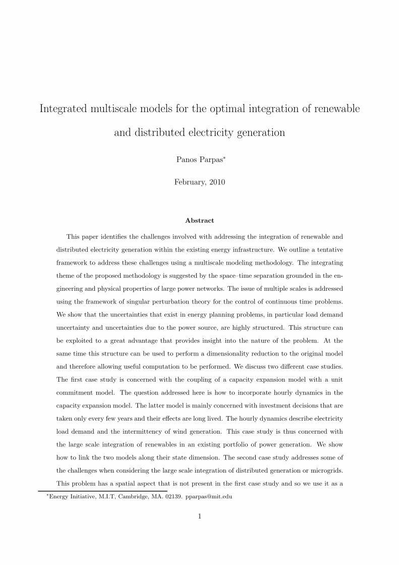
Integrated multiscale models for the optimal integration of renewable
and distributed electricity generation
Panos Parpas∗
February, 2010
Abstract
This paper identifies the challenges involved with addressing the integration of renewable and
distributed electricity generation within the existing energy infrastructure. We outline a tentative
framework to address these challenges using a multiscale modeling methodology. The integrating
theme of the proposed methodology is suggested by the space–time separation grounded in the en-
gineering and physical properties of large power networks. The issue of multiple scales is addressed
using the framework of singular perturbation theory for the control of continuous time problems.
We show that the uncertainties that exist in energy planning problems, in particular load demand
uncertainty and uncertainties due to the power source, are highly structured. This structure can
be exploited to a great advantage that provides insight into the nature of the problem. At the
same time this structure can be used to perform a dimensionality reduction to the original model
and therefore allowing useful computation to be performed. We discuss two different case studies.
The first case study is concerned with the coupling of a capacity expansion model with a unit
commitment model. The question addressed here is how to incorporate hourly dynamics in the
capacity expansion model. The latter model is mainly concerned with investment decisions that are
taken only every few years and their effects are long lived. The hourly dynamics describe electricity
load demand and the intermittency of wind generation. This case study is thus concerned with
the large scale integration of renewables in an existing portfolio of power generation. We show
how to link the two models along their state dimension. The second case study addresses some of
the challenges when considering the large scale integration of distributed generation or microgrids.
This problem has a spatial aspect that is not present in the first case study and so we use it as a
∗Energy Initiative, M.I.T, Cambridge, MA. 02139. [email protected]
1

template to illustrate how one could approach problems with a strong spatial component using a
multiscale framework.
1 Introduction
Due to the manifold of technoeconomic issues that arise in energy planning, the electricity industry
has for a long time relied on complex optimization models to perform its planning. Examples of such
models include unit commitment (decisions on which generators to use), economic dispatch (decide
the optimal level of use for each generator), capacity expansion (decide the optimal generation mix
to meet demand), hydro/thermal scheduling models, optimal power flow models and so on. While
there exists a large body of literature to address the range of challenges faced by the energy industry,
the environment in which these models are used is becoming increasingly complex. This complexity
is driven primarily by two factors. The first factor is the deregulation and re-regulation of electricity
markets. The second driver is the increasing pressure placed on the electricity industry to address
the problem of meeting demand in a sustainable manner. In order to deal with this complexity either
simplified models or heuristic methods are typically used. These approximations, are to a large extend,
uncontrolled and may have a substantial impact on the nature of the obtained solution. In particular
most models ignore the fact that many features, that have important ramifications for the selection of
the optimal policy, exist along multiple temporal and spatial scales. The impact of the optimization
methodology, and the potential inefficiencies of the old heuristics can be seen by two examples taken
from [Bloom, 2009]. The first is from Red Electrica de Espana (rEE), the Spanish national power
distributor. They switched from using heuristic models to an exact optimization methodology and
saved about 50k€-100k€ daily, and reduced emissions by about 2.5% annually (about 100,000 tons of
CO2). A second examples is a large system operator in the east of the United States that saved about
$200 million annually by solving the unit commitment problem by a branch and bound algorithm as
opposed to the heuristic method they used before. These examples illustrate the impact that ad hoc
heuristics can have on the energy industry. Incorporating large amounts of intermittent renewable
generation resources or the integration of distributed sources of electricity generation, makes an already
complex problem more complex. It is therefore important to have robust models that can scale, both
computationally and conceptually, with the increasingly complex issues faced in the energy industry.
2

This paper identifies the challenges involved with addressing the integration of renewable and
distributed electricity generation within the existing energy infrastructure. We outline a tentative
framework to address these challenges using a multiscale modeling methodology. The integrating
theme of the proposed methodology is suggested by the space–time separation grounded in the engi-
neering and physical properties of large power networks. Before we delve into the proposed modeling
methods it is necessary to decompose the implications of the two drivers and sources of the complexity
in which planning decision need to be taken. We refer the interested reader to [Claudio et al., 2008]
for a more complete discussion of these issues. Below we summarize the issues that have repercussions
on the planning models discussed in this paper.
2 Background
The deregulation of the industry means that utilities now have to compete in an open market envi-
ronment. The degree of deregulation varies from country to country, and from state to state in the
US. Despite these variations between regions, as well as the fact that real-time system operation is
still largely a centralized activity, deregulation has completely changed the way electricity generation
and long term planning are performed. In a regulated environment the utilities would pass on the
costs of any risks in generation costs directly to consumers. This approach is no longer possible in an
open market. Consequently, utilities see generation plants as an asset that needs to be risk managed
and optimally utilized. The focus is no longer on cost minimization, but on how to deliver a quality
product in an economically viable manner. However, electricity is different from other assets since
large scale storage is not economically feasible and so it needs to be generated and transmitted at the
same time it is needed. Thus the utility needs to maintain an equilibrium between generation and
demand in a way that ensures the safety and stability of the system, while maximizing asset utilization
at the same time. An important implication of the non-storability of electricity for long term planing,
is that it is not enough to know the total electricity needed, but also when it is needed. A system
under constant demand has dramatically different optimal design than a system facing a demand pro-
file with substantial variations over time. This property of electrical power system design remains the
same even if the total demand required is the same but the demand profile over time is different. One
way to address both the increasing volatility in generation costs as well as the way utilities respond
3

to variations in load is via investing in a portfolio of generation facilities. For example, nuclear plants
have large upfront investment costs, generally lower fuel costs, and are ideal for serving base load.
On the other end of the spectrum, gas turbines are cheap to build but have high fuel costs, and can
be used to meet peak demand. Utilities have also ventured, with mixed results [Parsons, 2008], into
trading. The reason behind the change of business model was either for hedging, risk management
purposes or so as to establish an alternative source of income. Thus considering a large and diverse
number of technologies and economic activities is an important facet of long term planning in the
energy sector. In a nutshell, the consequences of deregulation to capacity expansion decisions are the
increased need to incorporate robust methods for handling uncertainty and the importance of model-
ing load variations. Both of these factors are important if a substantial increase in system efficiency is
to be achieved. All these new facets of the capacity expansion problem need to be considered in view
of many possible current and evolving technologies. It is no longer possible to model each decision
in isolation. A system wide view encompassing not only physical, operational, and safety constraints
but also economic and, as it will be discussed next, environmental constraints as well, is required.
Until recently, and to a large extend even now, the environmental costs of producing electricity have
not been incorporated fully into the price consumers see. The process of internalizing these costs into
the price is currently under way. This requires utilities to think differently about some technologies,
and their role in helping make the transition into a system that can grow sustainably. For example, if
a utility wants to investigate the possibility of including a large amount of wind generation capacity
into their power portfolio, then due to the intermittent nature of wind, daily variations in load and
daily variations in wind speeds become more important. These daily variations will affect the way the
utility manages its reserves, and therefore effects the whole portfolio of generating capacity. Since the
output from a wind turbine increases by the cube of wind speed, using average wind speed will always
underestimate the amount of output available from wind and this can lead to an inefficient system
design. Again a system wide view needs to be taken. Currently, there exist little understanding on
how to, rigorously, capture these daily effects into long term planning.
The rest of this paper is structured as follows: in Section 3 we describe the general framework
we propose in order to capture some of the multiscale challenges described above. In Section 4 we
discuss a case study that couples capacity expansion with a unit commitment model. The results from
4
section 4 are taken from [Parpas and Webster, 2010]. In Section 5 we attempt to apply the methods
from [Parpas and Webster, 2010] to a distributed network planning problem. The analysis in 5 is both
speculative and exploratory in nature. We conclude in Section 6.
3 Overview of the proposed framework
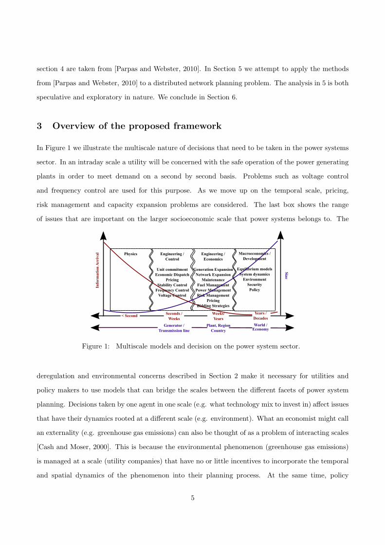
In Figure 1 we illustrate the multiscale nature of decisions that need to be taken in the power systems
sector. In an intraday scale a utility will be concerned with the safe operation of the power generating
plants in order to meet demand on a second by second basis. Problems such as voltage control
and frequency control are used for this purpose. As we move up on the temporal scale, pricing,
risk management and capacity expansion problems are considered. The last box shows the range
of issues that are important on the larger socioeconomic scale that power systems belongs to. The
Info
rm
ati
on
Arr
iva
l
Seconds /
Weeks< Second
Weeks/
Years
Years /
Decades
Engineering /
Control
Unit commitment
Economic Dispatch
Pricing
Stability Control
Frequency Control
Voltage Control
Physics Engineering /
Economics
Generation Expansion
Network Expansion
Maintenance
Fuel Management
Power Management
Risk Management
Pricing
Bidding Strategies
Macroeconomics /
Development
Equilibrium models
System dynamics
Environment
Security
Policy
Size
Generator /
Transmission line
Plant, Region
Country
World / Economy
Figure 1: Multiscale models and decision on the power system sector.
deregulation and environmental concerns described in Section 2 make it necessary for utilities and
policy makers to use models that can bridge the scales between the different facets of power system
planning. Decisions taken by one agent in one scale (e.g. what technology mix to invest in) affect issues
that have their dynamics rooted at a different scale (e.g. environment). What an economist might call
an externality (e.g. greenhouse gas emissions) can also be thought of as a problem of interacting scales
[Cash and Moser, 2000]. This is because the environmental phenomenon (greenhouse gas emissions)
is managed at a scale (utility companies) that have no or little incentives to incorporate the temporal
and spatial dynamics of the phenomenon into their planning process. At the same time, policy
5

instruments (e.g. carbon taxes) are designed with the purpose of mitigating long term environmental
impacts but also have an impact on the choice of technologies and amount of innovation at the firm
level. This type of technological change is not captured in large economic models concerned with
the long time scales. The problem is more complicated than what is shown in Figure 1. Agents on
different scales use different models and with different resolutions. For example, an economist may
use a detailed model of the US economy but only an approximated model for the EU economy. This
multi-model environment introduces additional complications that is beyond the scope of this paper.
Hitherto the problem of bridging the scales has been handled using ad-hoc methods e.g. [Wing, 2006,
Bohringer and Rutherford, 2008]. The objective of this paper is to describe a methodology to address
some aspects of this problem.
The modeling approach proposed in this paper is based on the observation that information per-
taining the issues on the left of Figure 1 arrive at a much faster rate than the information concerning
the issues on the right of the figure. The idea is then to use this property of the problem to identify
an integrated way of approaching these issues that is self-consistent, and transparent. The primary
objective is not to produce more accurate numbers by incorporating intraday variations, but rather
define the representational structures that will allow qualitative and quantitative reasoning about the
effects of different time scales to take place. At the same time this structure can be used to perform
a dimensionality reduction on the original model and therefore allowing useful computation to be
performed.
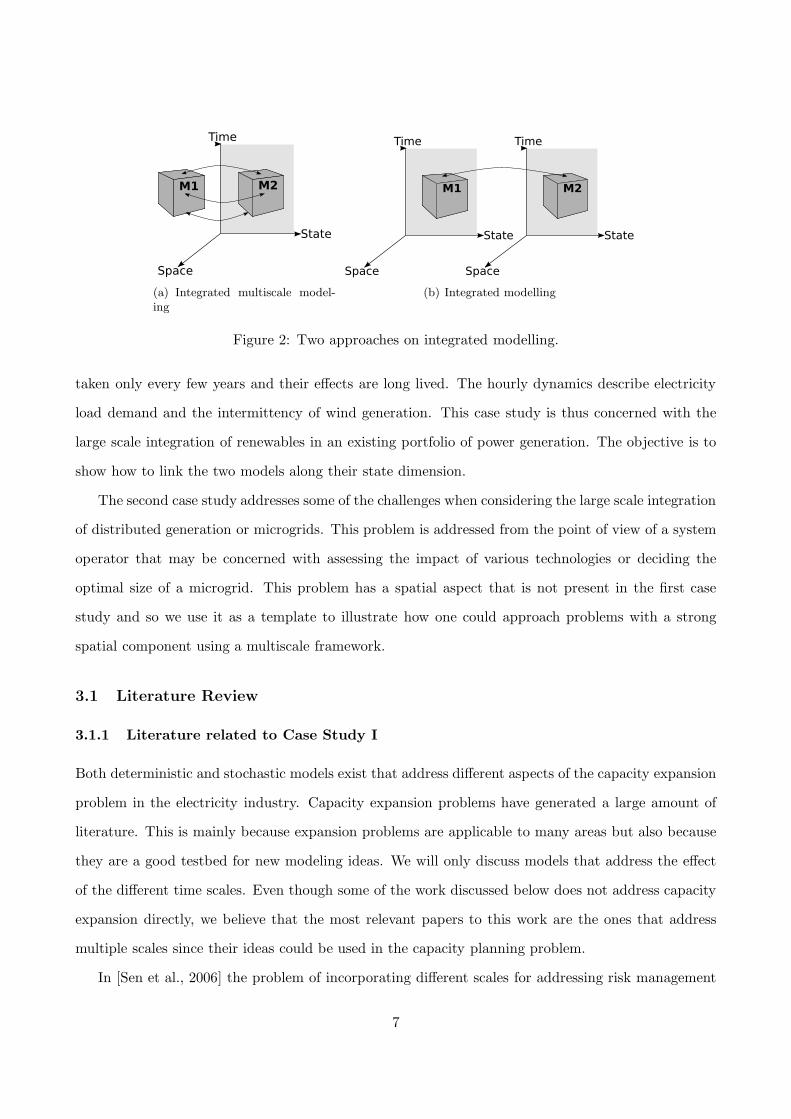
Figure 2(a) shows a pictorial representation of this research programme. Given two models M1 and
M2 that have different dynamics, the aim is to construct bridges along the spatial, temporal and state
dynamics of the two models. Figure 2(b) shows a different approach to integrated modeling where
each model has its own dynamics and the two models interact when needed, e.g. when the output of
one model is used as the input to the other. The proposed approach uses the conceptual framework of
figure 2(b). Both approaches offer viable solutions to integrated modeling. In order to be specific we
only discuss two case studies. These two problems provide a partial implementation of the programme
outlined above. The first case study is concerned with the coupling of a capacity expansion model with
a unit commitment model. The question addressed here is how to incorporate hourly dynamics in the
capacity expansion model. The latter model is mainly concerned with investment decisions that are
6
Time
State
Space
M1 M2
(a) Integrated multiscale model-ing
Time
State
Space
M1
Time
State
Space
M2
(b) Integrated modelling
Figure 2: Two approaches on integrated modelling.
taken only every few years and their effects are long lived. The hourly dynamics describe electricity
load demand and the intermittency of wind generation. This case study is thus concerned with the
large scale integration of renewables in an existing portfolio of power generation. The objective is to
show how to link the two models along their state dimension.
The second case study addresses some of the challenges when considering the large scale integration
of distributed generation or microgrids. This problem is addressed from the point of view of a system
operator that may be concerned with assessing the impact of various technologies or deciding the
optimal size of a microgrid. This problem has a spatial aspect that is not present in the first case
study and so we use it as a template to illustrate how one could approach problems with a strong
spatial component using a multiscale framework.
3.1 Literature Review
3.1.1 Literature related to Case Study I
Both deterministic and stochastic models exist that address different aspects of the capacity expansion
problem in the electricity industry. Capacity expansion problems have generated a large amount of
literature. This is mainly because expansion problems are applicable to many areas but also because
they are a good testbed for new modeling ideas. We will only discuss models that address the effect
of the different time scales. Even though some of the work discussed below does not address capacity
expansion directly, we believe that the most relevant papers to this work are the ones that address
multiple scales since their ideas could be used in the capacity planning problem.
In [Sen et al., 2006] the problem of incorporating different scales for addressing risk management
7

problems such as buying and selling forwards for fuel are addressed in conjunction with the intraday
unit commitment problem. Their model does not address intraday effects from intermittent sources.
They formulate the problem as a multistage stochastic programming problem. The resulting large scale
mixed integer linear programming problem is solved using a nested column decomposition algorithm.
In [Epe et al., 2009] the authors do address the problem of dealing with the intermittency of wind.
Again a multistage stochastic programming approach is taken and the resulting large scale optimization
problem is solved using a recombining tree methodology. In [Pritchard et al., 2005] the operation of a
hydro-electric reservoir is addressed. Their problem also has multiple scales since the supply of power
occurs intraday, in hourly intervals, but the management of the reservoir occurs over monthly scales.
The problem is formulated as a dynamic programming problem. By approximating the decision to
have some desirable properties the different scales can be decomposed. In [Powell et al., 2009] the
problem of multiple scales as well as the intermittency of wind and solar are handled using stochastic
dynamic programming. In order to solve the intractable dynamic programming problem approximate
dynamic programming is used. We refer to the review article in [Wallace and Fleten, 2003] and the
recent book [Weber, 2005] for a more complete overview of both stochastic programming approaches
as well as approaches based on dynamic programming. What all these papers have in common is that
they address the existence of multiple scales using some sort of algorithmic framework. They either
use a decomposition algorithm, approximate dynamic programming, or find some other way to relax
the non-anticipativity constraints in order to make the problem tractable.
To make operational the uncertainty structures present in this class of problems we make use of
the tools from singular perturbation theory for MDPs in continuous time. In some respects some
models already take advantage of this structure. For example the widely used MARKAL model
[Seebregts et al., 2001] uses the concept of a “typical” load to overcome the onerous requirement to
optimize over all possible loads. This type of heuristic is useful, but as we are trying to develop models
to understand the behavior of systems we do not observe it is important to understand why heuristics
work, when they fail, and what can be done instead. For example it is not clear how to extend these
heuristics to handle wind intermittency, or demand elasticity (a major objective of demand response
programs).
The main results for multiscale MDPs are summarized in two excellent books [Sethi and Zhang, 1994,
8

Yin and Zhang, 1998]. Therefore we only comment on the relations between this work and the lit-
erature. In [Jiang and Sethi, 1991] a similar model to ours is proposed. The model is motivated
by a manufacturing system with machines that have failure rates that occur on fast time scales.
However, their model does not address the issue of capacity expansion and demand is also determin-
istic. In [Zhang et al., 1997] another model similar to ours is proposed and is again studied in the
context of manufacturing systems. Their model also has fixed capacity and deterministic demand.
Even though the problem of capacity expansion with multiple scales has been studied, see Ch 10
in [Jiang and Sethi, 1991], their model does not address capacity expansion for Markov Chains with
weak interactions and multiple scales. Moreover all the papers described above are concerned mainly
with manufacturing systems, and in order to carry the results over to the power system sector we
had to devise a new framework. This is because in order to capture some of the basic features of the
energy planning models we needed a model that can handle a Markov chain with weak interactions
both on capacity (to model wind intermittency for example) as well as on the demand dynamics (to
model the demand load dynamics). We also need to handle uncertainties that are not changing fast,
such as the long term demand growth for electricity. In Section 4 we only provide an outline of these
extensions. The details can be found in [Parpas and Webster, 2010].
3.1.2 Literature related to Case Study II
The literature on network planning for power systems is vast. We refer the interested reader to
[Wallace and Fleten, 2003] and [Georgiadis et al., 2008] for a review. However there are currently
no studies that attempt to address the problem of optimal planning in the context of large scale
penetration of distributed generation technologies. There are a few studies that discuss the prob-
lem of a single network [Hawkes and Leach, 2009, Abu-Sharkh et al., 2006]. Some heuristic methods
for this problem are discussed in [Mendez et al., 2006]. In our analysis we rely on the results from
[Chow and Kokotovic, 1985]. The model discussed in [Chow and Kokotovic, 1985] pertains issues at a
smaller scale than the ones we propose to study. Also the work in [Chow and Kokotovic, 1985] has no
controls and is concerned with the deterministic case. We are interested in stochastic optimal control
problems.
9

4 Case Study I: State aggregation for capacity expansion
Before we delve into the details of the model, we first motivate our construction by looking at some of
the characteristics of some real electricity demand data. Hourly electricity load data time series have
a strong periodic component. By far the most widely used method to analyze such data sets is a two
step process. The first step involves identifying the periodic component in order to be able to remove
the trends that are related to time of day, weekend, and any other purely temporal elements. The
second step is to fit some stochastic process to the remaining component (we call this the stochastic
component). Hourly load data for 2007 were used from the PJM midatlantic region (PJM.E). This
data is freely downloadable from the PJM website.
Electricity hourly load demand is modeled as:
H(t) = D(t) + η0(t), t ∈ [0, T ]. (4.1)
The deterministic component is given by,
D(t) = a + bt +
N∑
j=0
cj cos(2πφjt + lj) t ∈ [0, T ]. (4.2)
Thus the deterministic component accounts for a linear trend in demand. The seasonal fluctuations
are super imposed around this linear trend. In our numerical experiments we used N = 5. The
deterministic harmonics of (4.2) are obtained from the peaks of the Fourier transform of the hourly
load data. In a more realistic model these parameters would be uncertain. The term η0 represents
the stochastic component. In order to identify a suitable stochastic process for η0 we fit a maximum
likelihood Markov Chain to the residual component. The residual component is given by,
r(t) = A(t) − D(t),
where A(t) represents the actual data (8760 points). The resulting transition matrix of the Markov
Chain is shown in Figure 3. The states in the Markov Chain represent the amount by which the
hourly load is above or below the deterministic periodic component (for ease of exposition the axis
shows the state number rather than the actual state). What is immediately obvious from this figure
10

is that apart from a few cases the Markov Chain will tend to stay around the same state. Of course
the variations around the state, as well as far away from the diagonal are important since they will
influence the amount of reserves. Figure 3(b) shows the result of the same process but with using
a Markov Chain with only ten states. Using typical states, optimizing over these and summing the
results, essentially assumes a transition matrix as in Figure 3(c) (an identity matrix). However using
typical states will always underestimate the costs of running such a system (this follows from Jensen’s
inequality and will be true for convex models, such as the one studied in this paper). This means that
a certain amount of guesswork will always be required in order to find the level of reserves, or any
other quantity of interest. Therefore, it seems that assuming the problem to be reducible to a few
typical states oversimplifies the problem. In view of the drive towards more efficient management of
increasingly scarce resources it is important to attempt to find better ways of incorporating hourly load
demand that leads to more realistic yet tractable models. Introducing uncertainty into demand load
management will give us a better understanding both of the true costs of the system as well as help
identify strategies to manage the dynamic equilibrium between supply and demand. At the same time
it is obvious from the figure that the data does not completely lack structure. To see the difference, a
process with no structure is shown in Figure 3(d). Therefore assuming a completely general structure
is also not appropriate. Methods that do not take advantage of this highly specialized feature of the
problem are essentially implicitly assuming a structure such as the one shown in Figure 3(d).
We followed a similar procedure for the wind data. We obtained wind data from the NCDC
[NCDC, 2009] website. The wind data contains the wind speeds at an hourly time interval over the
years 2007–2008, in the Buzzard’s bay area in south Massachusetts. The resulting Markov Chain for
wind uncertainty is shown in Figure 4.
The information structure proposed in this paper is shown in Figure 1. We start from the
bottom layer that has all the detailed intraday variations. This information is combined into ag-
gregate states. Finally some other probabilities are devised that control the transitions between
aggregate states. In order to make the structure in Figure 1 operational, we deploy the tools of
singular perturbation theory. Below we describe the main components of this framework. More infor-
mation can be found in [Yin and Zhang, 1998, Zhang et al., 1997, Phillips and Kokotovic, 1981] and
[Parpas and Webster, 2010].
11

(a) A Markov chain with 200 states (b) A Markov chain with 10 states
(c) (d) A structure free transition matrix
Figure 3: Markov transition matrices. (a)-(b) are obtained from a maximum likelihood fit to hourlytime series. (c) is the structure implicitly assumed when considering typical states. (d) was obtainedby a maximum likelihood fit to a white noise process.
12

(a) 20 states (b) 50 states
Figure 4: Markov transition matrices for wind uncertainty. (a)-(b) are obtained from a maximumlikelihood fit to hourly time series
Motivated by the data above we will assume a specific structure for the uncertainties representing
load demand and wind availability. To this end, the transition function is assumed to satisfy:
dP
dτ= p(τ)[Q + ǫW ],
p(0) = I.
(4.3)
where Q = diag(Q1, . . . , Qm). For the purposes of this section, we assume that the m aggregate states
have been identified by some statistical procedure. The ǫ parameter is used to make explicit the
assumption that the transitions inside one of the aggregate states are much more common than the
transitions between aggregate states. Since ǫ is assumed to be small, if we run the system for a small
amount of time then the W matrix will have a small role to play. However, if we run the system for
long periods then the transitions between aggregate states become significant. In order to capture the
latter effects, even as ǫ approaches 0, we stretch the time dimension t = ǫτ . This stretching of time
is what sets singular perturbations apart from regular perturbations. With this change of time (4.3)
13

becomes:
dP
dt= p(t)[
1
ǫQ + W ],
p(0) = I.
We note that we have not made any approximations so far. All we have assumed is that we can
identify the different aggregate states, and that we can specify an ǫ > 0 as a small parameter. This
parameter is used as a measure of the separation of scales. We are now in a position to fully specify
our model.
4.1 The model
We assume that the decision maker can use any of the N generating plants to meet demand
dx(t)
dt=
N∑
i
ui(t) − z(t) + η0(t, ǫ) x(0) = x. (4.4)
Where ui represents the output from the ith plant. x(t) represents the amount of energy not served.
We assume that some suitable penalty is imposed for meeting demand i.e. the cost of each unit of x
is high compared to the cost of production. z(t) represents the demand, and it is assumed to have the
following dynamics,
dz(t)
dt= f(z(t), ξ0(t)) z(0) = z. (4.5)
In (4.4) η0 is the fast scale Markov process that represents the intraday variations in hourly loads.
In (4.5) ξ0 is also assumed to be a finite state Markov process, but this process changes at a slower
rate. The latter process is used to represent uncertainties such as the long term trend demand for
electricity. Information about long term demand arrives at longer time intervals. Therefore it is not
appropriate to model this type of uncertainty as a fast scale process. We use the notation η and ξ, for
the fast, and slow scale dynamics throughout the paper.
We also assume that the decision maker can invest in each of the generating facilities with the
aim of increasing capacity. Some of the plants are allowed to have zero capacity to start with. The
14

cumulative investment, in the ith plant, is given by:
dyi(t)
dt= πi(t) yi(0) = yi, i = 1, . . . , N.
By imposing appropriate upper bounds on the rate of investment, πi, we can ensure that new capacity
cannot appear overnight. We assume that once total investment in plant i reaches level Ki then new
capacity becomes available. Each plant can be expanded once, and the level of investment required is
assumed to be deterministic. Both of these assumptions can be relaxed, but with significant increase
in the complexity of the analysis.
The total available capacity in the ith plant is assumed to be a Markov process, and it is given by:
ηi(ǫ, t) =
ηi1(ǫ, t) t ≤ τi
ηi2(ǫ, t − τi) t > τi
Where τi represents the stopping time:
τi = inf{t | yi(t) = Ki} ∧ T.
The states of ηi1(ǫ, t) and ηi
2(ǫ, t) are given by the set Si1 and Si
2 respectively. Where
Si1 = {si
1,1, si1,2, . . . , s
i1,mi
},
similar notation is used for Si2. We also assume that there exists a one-to-one mapping between states
in Si1 and Si
2, this will be denoted by κ : Si1 → Si
2. We use the notation Si to denote the states of
available capacity in the ith plant.
The Markov process η(t, ǫ) = [η0(t, ǫ), . . . , ηN (t, ǫ)] is assumed to have a generator given by:
dpη(t)
dt= pη(t)[W +
1
ǫQ] (4.6)
Where Q = diag(Q1, . . . , Ql). Furthermore both W and {Qi}li=1 are assumed to be irreducible. The
generator for the ξ variables can be much more general since we will not perform any approximation
15

on this process. The dynamics of ξ are given by,
dpξ(t)
dt= pξ(t)R.
A policy (u(t), π(t)) will be called admissible if it satisfies the dynamics specified above (including
the stochastic bounds on available capacity). Moreover an admissible policy needs to be adapted to
the filtration Ft. The set of all Ft-adapted processes is denoted by Aǫt. For notational simplification
we use w(t) = [x(t), y(t), z(t)] wherever possible.
The objective function and the complete problem are given below.
Jǫs(w, η, ξ;u, π) = E
{N∑
i=1
∫ T
s
e−ρ(t−s)Gi(xs, πi(s), ui(s), ξ(s))ds + e−ρ(T−s)φ(XT )
}
vs(w, η, ξ) = min Jǫs(w, η, ξ;u, π)
dx(t)
dt=
N∑
i
ui(t) − z(t) + η0(t, ǫ) x(s) = x
dz(t)
dt= f(z(t), ξ0(t)) z(s) = z
dy(t)
dt= π(t), y(s) = y (Hǫ)
yi(t) ≤ Ki
0 ≤ ui(t) ≤ ηi(t, ǫ)
(u(t), π(t)) ∈ Aǫt
Where Aǫt denotes the set of admissible controls. Note that the objective is allowed to depend on the
slow Markov process ξ. This may be used to represent uncertainties in operating costs (e.g. fuel costs,
emission costs etc.).
16

4.2 Asymptotic Analysis
As ǫ goes to zero, it can be shown [Parpas and Webster, 2010] that the value function of (Hǫ) is the
solution of the following aggregate problem.
vs(w, k, ξ) = min Js(w, k, ξ;u, π)
dx(t)
dt=
∑
j∈Mη(t)
λη(t)j
( N∑
i
uη(t),ji (s) − z(t) + η
η(t),j0
)x(s) = x
dz(t)
dt= f(z(t), ξ0(t)) z(s) = z
dy(t)
dt= π(t), y(s) = y (H)
yi(t) ≤ Ki
uη(t),ji (t) ∈ Ci(η(t), j)
η(s) = k.
Note that the value function is not a function of η but rather of the current aggregate state the process
is in. Ck(i, j) is the feasible set associated with the ith state inside the jth aggregate set of states for
technology k. In the case with no startup costs then this will simply be given by:
0 ≤ uη(t),ji (t) ≤ η
η(t),ji .
The expectation is taken with respect to the aggregated Markov Chain. That is the Markov Chain
that specifies the probability of moving between clusters of states. The complete derivation of the
approximate problem can be found in [Parpas and Webster, 2010]. The important feature in (H)
is that we only consider aggregate sets of states. This has significant computational advantages.
Additional numerical experiments from [Parpas and Webster, 2010] show that the algorithm used to
solve (H) requires a lot less iterations to converge than when the same algorithm is used on the
original problem. This is because of the so called smoothing property for such problems. We refer the
interested reader to [Parpas and Webster, 2010] for the details.
17

5 Case Study II: Spatial aggregation for distributed generation plan-
ning
Traditionally the physical flow of electricity has been fixed and centrally managed. Large generating
plants (hydro, nuclear or fossil-fired) generate power, and through the high voltage transmission net-
work, it reaches the low voltage network and eventually gets distributed to consumers. The economics
of power generation made this mode of operation efficient. Deregulation, concerns over environmental
impacts of power generation and security issues are challenging this traditional structure of power
generation. Distributed generation is the term used to describe a set of technologies that are located
close to the load demand centers. Since these distributed resources are not centrally managed they
pose a fresh set of challenges for the modeling of power grids. The term microgrid is used to de-
scribe a set of decentralized technologies operating to provide heat and power to a small set of mostly
residential customers. The technologies used in microgrids include both renewables sources such as
solar, wind, but also fossil-fuel based generators. A distinctive feature of microgrids is the empha-
sis on polygeneration. A microgrid can operate in isolation to the large national grid. It may also
operate in tandem with the main grid. The tandem operation will be needed if the microgrid can
not generate enough local power to satisfy local demand, or when too much power is generated and
then it can be sold back to the main grid. More information on the engineering aspects of distributed
generation can be found in [Masters, 2004]. Most studies have looked at the impact of a single mi-
crogrid (e.g. [Hawkes and Leach, 2009, Abu-Sharkh et al., 2006]). With some notable exceptions (see
[Mendez et al., 2006]) the large scale integration of microgrids has not been sufficiently analyzed. The
aim of this section is to show how a large number of microgrids can be analyzed together using similar
techniques as in Section 4.
5.1 The model
The first step in extending the techniques of section 4 is to endow the Markov process, representing the
load demand or any other uncertain quantity such as the availability of wind, with a spatial structure.
This class of stochastic processes are called random fields, see e.g. [Whittle, 1986]. Random fields
have been studied extensively. The optimal control of Markov random fields has received very little
attention compared with the standard Markov decision processes. Most of the work on the control of
18

spatial Markov processes is reviewed in [Chornei et al., 2006].
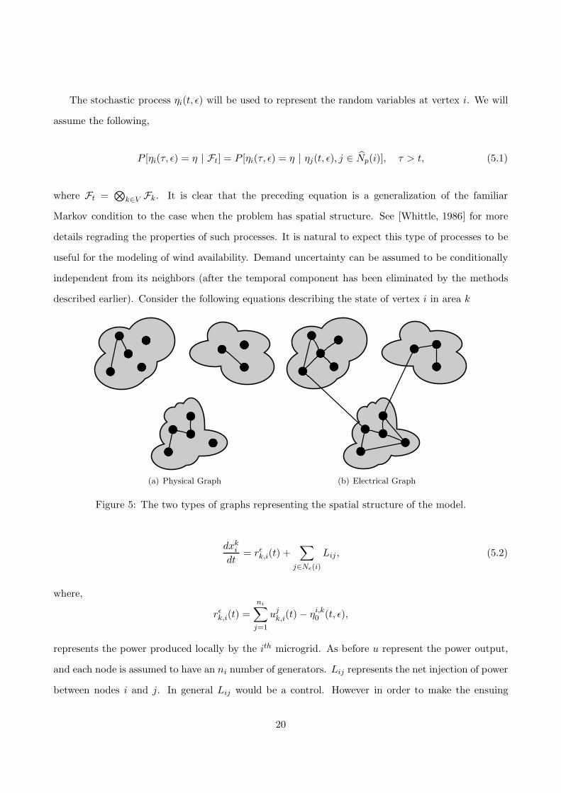
Let Γ = (V,Be, Bp) denote an undirected graph, where V denotes the set of vertices, and Bp
the set of physical edges, and Be the electrical edges. A physical edge exists between each node if
there is conditional dependency (in the sense defined below) between two nodes. An electrical edge
between two nodes means that a node is electrically connected with another node. Obviously this
is an idealization of how a large electrical network might be connected, however when attempting to
incorporate large amounts of intermittent wind generation it becomes important to separate the two
concepts. The graph is illustrated in Figure 5. The electrical graph should be easy to identify given
the actual configuration of the network. The graph related to the physical aspects of the network may
be different, even though one would expect that nodes that are close to each other should belong to the
same neighborhood. Each node on the graph will represent a single source of distributed generation.
Depending on the application this may be down to a single microgrid or a cluster of microgrids.
By k ↔ j we denote that vertex j is connected to vertex k. For each k ∈ Bp we define the set
Np(k) = {j ∈ Bp | k ↔ j} as the set of all neighboring vertices to vertex k. We use Np(k) = Np(k)∪k.
We use similar notation for Be. We further assume that the graph can be split into l different areas.
We use Mk to denote the set of nodes in area k.
At each node on the graph we use cIi (cE
i ) to denote the number of internal (external) connections
at node i. We define,
cI = mini{cI
i } cE = maxi
{cEi } ǫ1 =
cE
cI.
Therefore as ǫ1 gets smaller, one would expect to be able to analyze each area of the graph separately
without much loss of information. Next we define sparsity parameters for each area. We use sIk (sE
k )
to denote the number of internal (external) connections in area k. We use m = mink{|Mk|}. As in
the case of the node sparsity parameter we also define,
sI = mink
{sIk} sE = max
k{sE
k } ǫ2 =sE
mcI.
Intuitively, one would expect to be able to analyze each area separately when ǫ1 and ǫ2 are small
enough. Similar techniques as in the previous section could be used. In what follows we formulate a
simple network in order to make this operational.
19
The stochastic process ηi(t, ǫ) will be used to represent the random variables at vertex i. We will
assume the following,
P [ηi(τ, ǫ) = η | Ft] = P [ηi(τ, ǫ) = η | ηj(t, ǫ), j ∈ Np(i)], τ > t, (5.1)
where Ft =⊗
k∈V Fk. It is clear that the preceding equation is a generalization of the familiar
Markov condition to the case when the problem has spatial structure. See [Whittle, 1986] for more
details regrading the properties of such processes. It is natural to expect this type of processes to be
useful for the modeling of wind availability. Demand uncertainty can be assumed to be conditionally
independent from its neighbors (after the temporal component has been eliminated by the methods
described earlier). Consider the following equations describing the state of vertex i in area k
(a) Physical Graph (b) Electrical Graph
Figure 5: The two types of graphs representing the spatial structure of the model.
dxki
dt= rǫ
k,i(t) +∑
j∈Ne(i)
Lij , (5.2)
where,
rǫk,i(t) =
ni∑
j=1
ujk,i(t) − η
i,k0 (t, ǫ),
represents the power produced locally by the ith microgrid. As before u represent the power output,
and each node is assumed to have an ni number of generators. Lij represents the net injection of power
between nodes i and j. In general Lij would be a control. However in order to make the ensuing
20

analysis tractable we will assume that,
Lij = Lij(xi − xj).
Note that this function must satisfy an energy balance condition,
∑
i
∑
j∈Ne(i)
Lij = 0.
To help make the analysis concrete we assume the following,
Lij =
λij(xj − xi) if i ↔ j
0 otherwise
The general case of nonlinear functions can be handled in a similar way as in [Chow, 1982]. Under
these assumptions the system in (5.2) can now be written as,
dxki
dt= rǫ
k,i(t) +∑
j∈Mk
∑
j 6=i
λij(xkj − xk
i ) +
l∑
m6=k
∑
j∈Mm
λij(xkj − xk
i ). (5.3)
Motivated by the decomposition above, we define LI ∈ Rn×n to be a matrix containing the internal
connections in an area. This implies that LI must be block diagonal. The diagonal entries in this
matrix are chosen to satisfy,
LIii = −
∑
j∈Mk
λij ∀i ∈ Mk ∀k.
The off-diagonal entries of LI are chosen to equal λij provided that i and j belong to the same group.
Similarly we define LE ∈ Rn×n to be a matrix containing external connections. Thus LE satisfies the
following two conditions,
ΛEij =
λij if i 6= j and i ∈ Mk, j ∈ Mm m 6= k
−∑
m6=k
∑j∈Mm
λij if i = j, i ∈ Mk
0 otherwise.
21

Note that by definition L = LI + LE . With the definitions given above we can decompose the system
into its external and internal connections.
dx
dt= rǫ(t) + (LI + LE)x(t), . (5.4)
Define the following aggregate variable,
yk =
|Mk|∑
i=1
xki
|Mk|=
1
|Mk|1T|Mk|
xk,
where 1n denotes a vector of ones of dimension n. We can vectorize the expression above as follows,
y = Cx.
Where,
C , M−1UT ∈ Rl×n,
U , diag(1|M1|, . . . ,1|Ml|) ∈ Rn×n,
M , diag(|M1|, . . . , |Ml|) ∈ Rl×l.
Next we define the first node in each neighborhood as a reference node,
zki−1 = xk
i − xki−1 i = 2, . . . ,Mk.
We will use z = Gx, to denote the equation above in vector form. The matrix G is defined in the
obvious way. It is shown in the Appendix that after some change of variables the following scaled
system can be derived,
dy
dτ= G1r
ǫ(t) + A1y + A2z
ǫ2dz
dτ= G1r
ǫ(t) + ǫ1B1y + B2z.
It can be seen from the system above that ǫ2 is a singular perturbation parameter, while the parameter
ǫ1 serves the role of a regular perturbation parameter. The significance of the system in 5.1 is that it
22

represents a controlled approximation of the aggregated dynamics of the original system. As there are
three small parameters for this problem1, the asymptotic analysis as these parameters tend to zero is
much more complicated. Despite the increased complexity there are several ways one could proceed.
One could solve the optimal control problem by letting ǫ approach to zero. At this limit the dynamics
representing the uncertainties in net power flow in each area would be obtained. The solution will
contain two sources of error. The first is due to taking the limit ǫ → 0. The second source of error is
due to using the aggregated dynamics instead of the correct dynamics. Error estimates for the latter
source of error could then be derived using standard techniques (see e.g. [Chow and Kokotovic, 1985]).
Due to space limitations we omit the detailed implementation of this approach. The details will appear
elsewhere.
6 Conclusions
Optimization models have been used in the electric power industry for a long time. Environmental
considerations and the development of new distributed generation technologies make it necessary to
consider the properties of power networks at multiple scales and from the point of view of multiple
agents. This paper proposed a tentative framework to address some of these challenges.
Appendix
In the Appendix we show how the perturbed dynamics in (5.1) are derived. These calculation were
done in [Chow and Kokotovic, 1985]. One difference in the computations below is the existence of
control variable representing the net injection of power in a node. The other difference is the existence
of uncertainty. Using the same notation as in Section 5, we obtained the following two expressions for
the nodes on the graph,
y = Cx z = Gx,
It follows from [Aoki, 1968] that we can derive the following expression for x,
x = Uy + Wz,
1Remember that ǫ is the singular perturbation parameter for the uncertainties around net power injection.
23
where W = GT (GGT )−1. It follows that,
dy
dt= C
dx
dt= C(rǫ(t) + (LI + LE)x(t))
= C(rǫ(t) + (LI + LE)(Uy(t) + Wz(t)))
= Crǫ(t) + CLEUy(t) + CLEWz(t).
(6.1)
Similarly, for z we obtain the following,
dz
dt= G
dx
dt= G(rǫ(t) + (LI + LE)x(t))
= Grǫ(t) + GLEUy(t) + (GLEW + GLIW )z(t).
(6.2)
The significance of the reformulation of the system above is that the matrix with the internal links
LI appears only in the last expression in the system above. Next we observe that if ǫ1 and ǫ2 are
sufficiently small2 then one would expect the norm of (GLEW + GLIW ) to be much larger than the
other matrixes in (6.1) and (6.2). This motivates the following change of time t1 = ǫ1t. We also rescale
the matrices to that everything is of O(1). We use the following definitions,
A1 ,CLEU
cIǫ2A2 ,
CLEW
cIǫ2
B1 ,GLEU
cIǫ1B2 ,
G(LI + LE)W
cI.
G1 ,G
cI
With the rescaled dynamics introduced above we obtain the following dynamics,
dx
dt1= ǫ2G1r
ǫ(τ) + ǫ2A1y + ǫ2A2z
dz
dt1= G1r
ǫ(τ) + ǫ1B1y + B2z.
The final system is obtained by rescaling the system above in its slow time scale,
τ = ǫ2t1
2Remember that ǫ1 is the perturbation parameter representing the ratio of external to internal connection in aneighborhood. The other parameter ǫ2 represents the permutation parameter that represents the sparsity of the graphin relation to the number of nodes and number of internal connections.
24

dx
dτ= G1r
ǫ(t) + A1y + A2z
ǫ2dz
dτ= G1r
ǫ(t) + ǫ1B1y + B2z.
References
[Abu-Sharkh et al., 2006] Abu-Sharkh, S., Arnold, R., Kohler, J., Li, R., Markvart, T., Ross, J.,
Steemers, K., Wilson, P., and Yao, R. (2006). Can microgrids make a major contribution to UK
energy supply? Renewable and Sustainable Energy Reviews, 10(2):78–127.
[Aoki, 1968] Aoki, M. (1968). Control of large-scale dynamic systems by aggregation. IEEE Trans-
actions on Automatic Control, 13(3):246–253.
[Bloom, 2009] Bloom, J. (2009). Optimization Applications in the Energy and Power Industries.
http://www-01.ibm.com/software/websphere/industries/energy/.
[Bohringer and Rutherford, 2008] Bohringer, C. and Rutherford, T. (2008). Combining bottom-up
and top-down. Energy Economics, 30(2):574–596.
[Cash and Moser, 2000] Cash, D. and Moser, S. (2000). Linking global and local scales: designing
dynamic assessment and management processes. Global Environmental Change, 10(2):109–120.
[Chornei et al., 2006] Chornei, R., Daduna, H., and Knopov, P. (2006). Control of spatially structured
random processes and random fields with applications. Springer Verlag.
[Chow, 1982] Chow, J. (1982). Time-scale modeling of dynamic networks with applications to power
systems. Springer-Verlag.
[Chow and Kokotovic, 1985] Chow, J. and Kokotovic, P. (1985). Time scale modeling of sparse dy-
namic networks. IEEE Transactions on Automatic Control, 30(8):714–722.
[Claudio et al., 2008] Claudio, C., Gomez-Exposito, A., Conejo, A., Canizares, C., and Antonio, G.
(2008). Electric Energy Systems: Analysis and Operation. CRC.
[Epe et al., 2009] Epe, A., Kuchler, C., Romisch, W., Vigerske, S., Wagner, H., Weber, C., and Woll,
O. (2009). Optimization of Dispersed Energy Supply-Stochastic Programming with Recombining
Scenario Trees. Optimization in the Energy Industry, page 347.
25

[Georgiadis et al., 2008] Georgiadis, M., Pistikopoulos, E., and Kikkinides, E. (2008). Energy Systems
Engineering: Volume 5: Energy Systems Engineering. Wiley-VCH.
[Hawkes and Leach, 2009] Hawkes, A. and Leach, M. (2009). Modelling high level system design and
unit commitment for a microgrid. Applied Energy, 86(7-8):1253–1265.
[Jiang and Sethi, 1991] Jiang, J. and Sethi, S. (1991). A state aggregation approach to manufacturing
systems having machine states with weak and strong interactions. Operations Research, 39(6):970–
978.
[Masters, 2004] Masters, G. (2004). Renewable and efficient electric power systems. Wiley, Inter-
science.
[Mendez et al., 2006] Mendez, V., Rivier, J., Fuente, J., Gomez, T., Arceluz, J., Marin, J., and
Madurga, A. (2006). Impact of distributed generation on distribution investment deferral. In-
ternational Journal of Electrical Power and Energy Systems, 28(4):244–252.
[NCDC, 2009] NCDC (2009). National Climatic Data Center,
http://www.ncdc.noaa.gov/oa/ncdc.html.
[Parpas and Webster, 2010] Parpas, P. and Webster, M. (2010). A singular perturbation approach to
multiscale power system capacity expansion. Submitted.
[Parsons, 2008] Parsons, J. (2008). Do Trading and Power Operations Mix? The Case of Constellation
Energy Group 2008. Massachusetts Institute of Technology, Working Papers, Center for Energy and
Environmental Policy Research.
[Phillips and Kokotovic, 1981] Phillips, R. and Kokotovic, P. (1981). A singular perturbation ap-
proach to modeling and control of Markov chains. IEEE Transactions on Automatic Control,
26(5):1087–1094.
[Powell et al., 2009] Powell, W., George, A., Lamont, A., and Stewart, J. (2009). SMART: A Stochas-
tic Multiscale Model for the Analysis of Energy Resources, Technology and Policy. Preprint.
[Pritchard et al., 2005] Pritchard, G., Philpott, A. B., and Neame, P. J. (2005). Hydroelectric reservoir
optimization in a pool market. Math. Program., 103(3, Ser. A):445–461.
26

[Seebregts et al., 2001] Seebregts, A., Goldstein, G., and Smekens, K. (2001). Energy/environmental
modeling with the MARKAL family of models. In Proc. Int. Conf. on Operations Research (OR
2001).
[Sen et al., 2006] Sen, S., Yu, L., and Genc, T. (2006). A stochastic programming approach to power
portfolio optimization. Oper. Res., 54(1):55–72.
[Sethi and Zhang, 1994] Sethi, S. P. and Zhang, Q. (1994). Hierarchical decision making in stochastic
manufacturing systems. Systems & Control: Foundations & Applications. Birkhauser Boston Inc.,
Boston, MA.
[Wallace and Fleten, 2003] Wallace, S. and Fleten, S. (2003). Stochastic programming in energy. In
A., R. and A., S., editors, Handbooks in OR & MS, chapter 10. Elsevier Science.
[Weber, 2005] Weber, C. (2005). Uncertainty in the electric power industry: methods and models for
decision support. Springer Verlag.
[Whittle, 1986] Whittle, P. (1986). Systems in stochastic equilibrium. John Wiley & Sons, Inc. New
York, NY, USA.
[Wing, 2006] Wing, I. (2006). The synthesis of bottom-up and top-down approaches to climate policy
modeling: Electric power technologies and the cost of limiting US CO2 emissions. Energy Policy,
34(18):3847–3869.
[Yin and Zhang, 1998] Yin, G. G. and Zhang, Q. (1998). Continuous-time Markov chains and ap-
plications, volume 37 of Applications of Mathematics (New York). Springer-Verlag, New York. A
singular perturbation approach.
[Zhang et al., 1997] Zhang, Q., Yin, G., and Boukas, E. (1997). Controlled Markov chains with weak
and strong interactions: asymptotic optimality and applications to manufacturing. Journal of
Optimization Theory and Applications, 94(1):169–194.
27