integrated planning and control for convex-bodied nonholonomic … · integrated planning and...

Integrated Planning and Control for Convex-bodiedNonholonomic systems using Local Feedback Control Policies

David C. Conner, Alfred A. Rizzi, and Howie Choset

CMU-RI-TR-06-34

August 2006

Robotics InstituteCarnegie Mellon University

Pittsburgh, Pennsylvania 15213

c 2006 Carnegie Mellon University

Abstract

We present a method for defining a hybrid control system capable of simultaneously addressing theglobal navigation and control problem for a convex-bodied wheeled mobile robot navigating amongst obsta-cles. The method uses parameterized continuous local feedback control policies that ensure safe operationover local regions of the free configuration space; each local policy is designed to respect nonholonomicconstraints, bounds on velocities (inputs), and obstaclesin the environment. The hybrid control systemmakes use of a collection of these local control policies in concert with discrete planning tools in order toplan, and replan in the face of changing conditions, while preserving the safety and convergence guaran-tees of the underlying control policies. In this paper, we provide details of the system models and policydefinitions used to validate the approach in simulation and experiment with a convex-bodied wheeled mo-bile robot. This work is one of the first that combines formal planning with continuous feedback controlguarantees for systems subject to nonholonomic constraints, input bounds, and non-trivial body shape.

c 2006 Carnegie Mellon i

Contents

1 Introduction 1

2 Related Work 32.1 Motion Planning and Control with Nonholonomic Constraints . . . . . . . . . . . . . . . . 32.2 Sequential Composition . . . . . . . . . . . . . . . . . . . . . . . . . . .. . . . . . . . . . 4

3 General Framework 73.1 System Models . . . . . . . . . . . . . . . . . . . . . . . . . . . . . . . . . . . .. . . . . 73.2 Generic Policy Requirements . . . . . . . . . . . . . . . . . . . . . . .. . . . . . . . . . . 8

3.2.1 Simple Inclusion Tests . . . . . . . . . . . . . . . . . . . . . . . . . .. . . . . . . 83.2.2 Contained in Free Space . . . . . . . . . . . . . . . . . . . . . . . . . .. . . . . . 93.2.3 Conditionally Positive Invariant . . . . . . . . . . . . . . . .. . . . . . . . . . . . 103.2.4 Finite Time Convergence . . . . . . . . . . . . . . . . . . . . . . . . .. . . . . . . 10

3.3 Discrete Planning in Space of Policies . . . . . . . . . . . . . . .. . . . . . . . . . . . . . 113.3.1 Extensions to Prepares Definition . . . . . . . . . . . . . . . . .. . . . . . . . . . 113.3.2 Planning in Policy Space . . . . . . . . . . . . . . . . . . . . . . . . .. . . . . . . 12

4 Local Policy Definitions 154.1 Inclusion Test . . . . . . . . . . . . . . . . . . . . . . . . . . . . . . . . . . .. . . . . . . 184.2 Free Configuration Space Test . . . . . . . . . . . . . . . . . . . . . . .. . . . . . . . . . 184.3 Conditional Invariance Test . . . . . . . . . . . . . . . . . . . . . . .. . . . . . . . . . . . 194.4 Vector Field Definition and Convergence Test . . . . . . . . . .. . . . . . . . . . . . . . . 20

5 Policy Deployment Technique 23

6 Current Results 276.1 Robot System and Implementation . . . . . . . . . . . . . . . . . . . .. . . . . . . . . . . 276.2 Navigation Experiments . . . . . . . . . . . . . . . . . . . . . . . . . . .. . . . . . . . . 296.3 Task Level Planning Simulations . . . . . . . . . . . . . . . . . . . .. . . . . . . . . . . . 30

7 Conclusion 33

A Free Space Testing 37

References 41

c 2006 Carnegie Mellon iii

1 Introduction

The problem of simultaneously planning and controlling themotion of a convex-bodied wheeled mobilerobot in a cluttered planar environment is challenging because of the relationships among control, nonholo-nomic constraints, and obstacle avoidance. The objective is to move the robot through its environment suchthat it arrives at a designated goal set without coming into contact with any obstacle, while respecting thenonholonomic constraints and velocity (input) bounds inherent in the system.

Conventional approaches addressing this problem typically decouple navigation and control [12, 31, 33].First, a planner finds a path, and then a feedback control strategy attempts to follow that path. Often themethods assume a point or circular robot body; other non-trivial robot body shapes complicate the problemof finding a safe path, as the path must be planned in the free configuration space of the robot. This leaves thechallenging problem of designing a control law that converges to the one-dimensional path, while remainingsafe with respect to obstacles.

We address the coupled navigation and control problem by generating a vector field along which therobot can “flow.” Unfortunately, determining a global vector field that satisfies all of these objectives forconstrained systems can be quite difficult. Our approach, inspired by the idea ofsequential composition[11],uses a collection of local feedback control policies coupled with a switching strategy to generate the vectorfield. Composing these relatively simple policies induces apiecewise continuous vector field over the union ofthe policy domains. Apolicy is specified by a configuration dependent vector field defined over a local regionof the robot’s free configuration space, termed acell. From this vector field and knowledge of the currentrobot state, the control inputs are determined such that theclosed-loop dynamics flows to the specified policygoal set within the cell. Figure 1 shows four paths induced byinvoking the local policies for four differentinitial conditions in the robot experiments, as will be discussed in Section 6.

−5 0 5−5

−4

−3

−2

−1

0

1

2

3

4

5

x (meters)

y (m

eter

s)

1

2

3

4

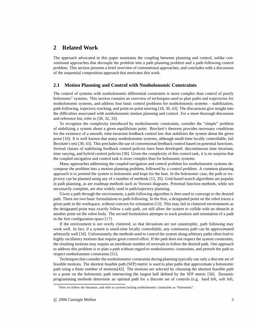
Figure 1: Experimental results of four robot runs using the proposed hybrid control framework. An explicitdesired path is never calculated, the path is induced by sequentially chaining local feedback control policiestogether; the policy ordering is determined by a discrete planner. The induced path preserves the localguarantees of the local polices, and is thus free of collision while respecting the system constraints.

c 2006 Carnegie Mellon 1

A discrete transition relation represented by a graph is induced by the transition between the domain ofone policy to the domain of a second policy containing the policy goal set of the first. On-line planning, andre-planning under changing conditions, becomes more tractable on the graph, allowing us to bring numerousdiscrete planning tools to bear on this essentially continuous problem. By sequencing the local policiesaccording to the ordering determined by a discrete planner,the closed loop dynamics induce the discretetransitions desired by the discrete plan. The overall hybrid (switched) control policy responds to systemperturbations without the need for re-planning. In the faceof changing environmental conditions, the discretegraph allows for fast online re-planning, while continuingto respect the system constraints.

By coupling planning and control in this way, the hybrid control system plans in the discrete space ofcontrol policies; thus, the approach represents a departure from conventional techniques. A “thin” path ortrajectory is never explicitly planned; instead, the trajectory induced by the closed-loop dynamics flows alongthe vector field defined by the active policy, which is chosen according to an ordering determined by a discreteplanner. A plan over the discrete graph associated with the collection of policies corresponds to a “thick” setof configurations within the domains of the associated localpolicies.

This approach offers guaranteed convergence over the unionof the local policy domains. For the methodto be complete, the entire free configuration space must be covered by policy domains (cells). This is adifficult problem due to the multiple constraints on the robot dynamics. Herein, the focus is on deploying a“rich enough” collection of policies that enables the navigation problem to be addressed over the bulk of thefree configuration space.

This paper describes the basic requirements that any local policy must satisfy to be deployed in thisframework; each local policy must be provably safe with respect to obstacles and guarantee convergenceto a specified policy goal set, while obeying the system constraints within its local domain. We develop aset of generic policies that meet these requirements, and instantiate these generic policies in the robot’s freeconfiguration space. The underlying equations are detailed, and examples are provided. Finally, a concretedemonstration of controlling a real mobile robot using a collection of local policies is described.

2 c 2006 Carnegie Mellon

2 Related Work

The approach advocated in this paper maintains the couplingbetween planning and control, unlike con-ventional approaches that decouple the problem into a path planning problem and a path-following controlproblem. This section presents a brief overview of conventional approaches, and concludes with a discussionof the sequential composition approach that motivates thiswork.

2.1 Motion Planning and Control with Nonholonomic Constraints

The control of systems with nonholonomic differential constraints is more complex than control of purelyholonomic1 systems. This section contains an overview of techniques used to plan paths and trajectories fornonholonomic systems, and address four basic control problems for nonholonomic systems – stabilization,path-following, trajectory-tracking, and point-to-point steering [18, 30, 43]. The discussions give insight intothe difficulties associated with nonholonomic motion planning and control. For a more thorough discussionand reference list, refer to [30, 32, 33].

To recognize the complexity introduced by nonholonomic constraints, consider the “simple” problemof stabilizing a system about a given equilibrium point. Brockett’s theorem provides necessary conditionsfor the existence of a smooth, time-invariant feedback control law that stabilizes the system about the givenpoint [10]. It is well known that many nonholonomic systems,although small-time locally controllable, failBrockett’s test [30, 43]. This precludes the use of conventional feedback control based on potential functions.Several classes of stabilizing feedback control policies have been developed: discontinuous time invariant,time varying, and hybrid control policies [30]. Given the complexity of this control task, it is no surprise thatthe coupled navigation and control task is more complex thanfor holonomic systems.

Many approaches addressing the coupled navigation and control problem for nonholonomic systems de-compose the problem into a motion planning problem, followed by a control problem. A common planningapproach is to pretend the system is holonomic and hope for the best. In the holonomic case, the path or tra-jectory can be planned using any of a number of methods [12, 35]. Grid-based search algorithms are popularin path planning, as are roadmap methods such as Voronoi diagrams. Potential function methods, while notnecessarily complete, are also widely used in path/trajectory planning.

Given a path through the environment, a path-following algorithm is then used to converge to the desiredpath. There are two basic formulations to path-following. In the first, a designated point on the robot traces agiven path in the workspace, without concern for orientation [15]. This may fail in cluttered environments asthe designated point may exactly follow a safe path, yet still allow the system to collide with an obstacle atanother point on the robot body. The second formulation attempts to track position and orientation of a pathin the free configuration space [17].

If the environment is not overly cluttered, so that deviations are not catastrophic, path following maywork well. In fact, if a system is small-time locally controllable, any continuous path can be approximatedarbitrarily well [34]. Unfortunately, the methods used to control the system along arbitrary paths often lead tohighly oscillatory motions that require great control effort. If the path does not respect the system constraints,the resulting motions may require an inordinate number of reversals to follow the desired path. One approachto address this problem is to plan a path without regard to nonholonomic constraints, and perturb the path torespect nonholonomic constraints [51].

Techniques that consider the nonholonomic constraints during planning typically use only a discrete set offeasible motions. The shortest feasible path (SFP) metric is used to plan paths that approximate a holonomicpath using a finite number of motions[42]. The motions are selected by choosing the shortest feasible pathto a point on the holonomic path intersecting the largest ball defined by the SFP metric [56]. Dynamicprogramming methods determine an optimal path for a discrete set of controls (e.g. hard left, soft left,

1Here we follow the literature, and refer to systems lacking nonholonomic constraints as “holonomic”.


straight, soft right, hard right) [3, 21, 36]. Probabilistic roadmaps (PRM) and rapidly-exploring randomtrees (RRT) are other discrete approaches to determining feasible paths for nonholonomically constrainedsystems [37, 54]. With the exception of dynamic programming, these discrete methods are not feedbackbased, and require replanning if the system deviates from the desired path.

Even if the planned path respects the nonholonomic constraints, the path must be followed by the robot.The presence of nonholonomic constraints renders path-following a non-linear controls problem. Controllaws based on a Lyapunov analysis [17] or feedback linearization [18, 50] are common. Most path-followingalgorithms assume continuous motion, with a non-stationary path defined for all time. This (temporarily)avoids Brockett’s problem with stabilization to a point [15, 17]. The path-following control policy asymptot-ically brings the error between the desired path and the actual path to zero. Typically, the control policy isconstructed for a specific vehicle and class of paths [2, 17, 15, 55].

The path-following control laws are unaware of environmental obstacles; therefore, for a nonzero initialerror or perturbation during motion, the system may collidewith an obstacle. Path-following may be coupledwith local obstacle avoidance, but this may invalidate the convergence guarantees. Thus, if the errors arelarge enough, the paths must be replanned, starting from thecurrent location.

In addition to path-planning, trajectories that specify when the system arrives at points along the path maybe planned [17, 50]. Trajectory-tracking problems can be problematic if the system is subject to a constraintthat delays the tracking [17]. In this case, the accumulatederror may make the system unstable or requireunreasonably high inputs. Another possible problem is thattrajectory-tracking controls may switch directionsfor certain initial conditions [50]. Unless the time matching along the trajectory is crucial, path-following isoften a better formulation [17, 50].

In related work, several methods – including sinusoidal inputs, piecewise constant inputs, optimal control,and differentially flat inputs – solve the point-to-point steering problem between two positions using openloop controls [34, 43]. These methods are sometimes incorporated into the discrete planning systems. Eachof these methods is an open loop control method that does not respect obstacles. Collision detection mustbe performed after the path is found to determine feasibility in a cluttered environment [27]. These point-to-point steering methods are strictly open loop, and not suitable for feedback control. The inevitable errorsnecessitate repeated applications to induce convergence to the goal point.

There have been a few attempts to address the coupled navigation and control problem for nonholonomicsystems. A method based on potential fields uses resistive networks to approximate the nonholonomic con-straints [14]. This approach requires a discretization of the configuration space, and is therefore subject tonumerical difficulties when calculating derivatives necessary for feedback control. Other approaches defineintegral sub-manifolds in configuration space that containthe goal [25, 29, 41]. On the sub-manifold, thenonholonomic constraints are integrable, and the control naturally respects the constraints. The approachesdrive the system to the sub-manifold, and then along the sub-manifold to the goal. While these methods aresuitable for feedback control implementations, determination of a suitable manifold is sometimes difficult.For systems where the stable manifold is not given in closed form, an iterative process is used to approximatethe manifold. The approaches also involve designing several functions that require insight into the specificproblem and system constraints.

2.2 Sequential Composition

The research presented in this paper uses the technique ofsequential composition, which enables the con-struction of switched control policies with guaranteed behavior and provable convergence properties [11].

The original form of sequential composition uses state regulating feedback control policies, whose do-mains of attraction partition the state space into cells [11]. The control policy can be thought of as a funnel,as shown in Figure 2, where the vertical represents the valueof a Lyapunov function, and the domain is the


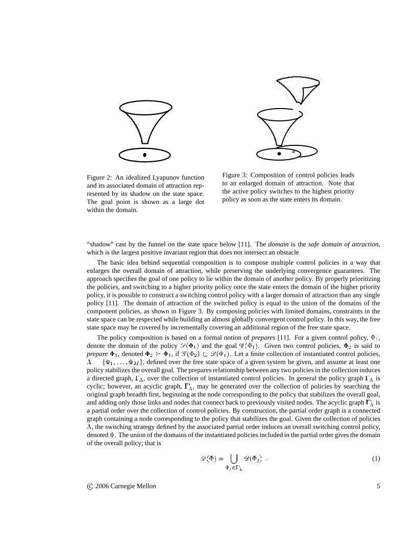
Figure 2: An idealized Lyapunov functionand its associated domain of attraction rep-resented by its shadow on the state space.The goal point is shown as a large dotwithin the domain.

Figure 3: Composition of control policies leadsto an enlarged domain of attraction. Note thatthe active policy switches to the highest prioritypolicy as soon as the state enters its domain.

“shadow” cast by the funnel on the state space below [11]. Thedomainis thesafe domain of attraction,which is the largest positive invariant region that does notintersect an obstacle

The basic idea behind sequential composition is to compose multiple control policies in a way thatenlarges the overall domain of attraction, while preserving the underlying convergence guarantees. Theapproach specifies the goal of one policy to lie within the domain of another policy. By properly prioritizingthe policies, and switching to a higher priority policy oncethe state enters the domain of the higher prioritypolicy, it is possible to construct a switching control policy with a larger domain of attraction than any singlepolicy [11]. The domain of attraction of the switched policyis equal to the union of the domains of thecomponent policies, as shown in Figure 3. By composing policies with limited domains, constraints in thestate space can be respected while building an almost globally convergent control policy. In this way, the freestate space may be covered by incrementally covering an additional region of the free state space.

The policy composition is based on a formal notion ofprepares[11]. For a given control policy,�1,denote the domain of the policyD(�1) and the goalG (�1). Given two control policies,�2 is said toprepare�1, denoted�2 � �1, if G (�2) � D(�1). Let a finite collection of instantiated control policies,� = f�1; : : : ;�Mg, defined over the free state space of a given system be given, and assume at least onepolicy stabilizes the overall goal. The prepares relationship between any two policies in the collection inducesa directed graph,��, over the collection of instantiated control policies. In general the policy graph�� iscyclic; however, an acyclic graph,�0�, may be generated over the collection of policies by searching theoriginal graph breadth first, beginning at the node corresponding to the policy that stabilizes the overall goal,and adding only those links and nodes that connect back to previously visited nodes. The acyclic graph�0� isa partial order over the collection of control policies. By construction, the partial order graph is a connectedgraph containing a node corresponding to the policy that stabilizes the goal. Given the collection of policies�, the switching strategy defined by the associated partial order induces an overall switching control policy,denoted�. The union of the domains of the instantiated policies included in the partial order gives the domainof the overall policy; that is D(�) = [�j2�0�D(�j) : (1)


The overall control policy induced by sequential composition is fundamentally a hybrid control policy [6,8, 24]. The composition of these local policies in a hybrid systems framework enables analysis on the discreterepresentation of the transitions between policy domains [8, 11]. We may analyze whether a goal node isreachable using the partial order graph��, which functions as a finite state automata [24]. Reachabilityof the goal state and decidability of the navigation problemfor a particular collection of policies can bedetermined by the discrete transitions on��, without analyzing the underlying continuous system [24].Thisanalysis may be done prior to, or during, construction of thepartial order.

The stability of the underlying control policies guarantees the stability of the overall switched policybecause the partial order results in monotonic switching [11]. This obviates the need for complex hybrid sta-bility analysis of the form given in [5, 7, 16, 38]. Disturbances are robustly handled provided their magnitudeand rate of occurrence is small compared to the convergence of the individual policies [11].

The system in [11] uses multiple policies to demonstrate theinherent robustness of the technique. Thedeployment of the generic policies – including specification of the setpoints, control policy gains, and pol-icy ordering – is accomplished manually. The deployment uses conservative approximations of the policydomains obtained through experimentation and simulation.

Sequential composition-like techniques have been appliedto mobile robots. Many examples are forsystems without nonholonomic constraints, where the policies are defined over simple cells – polytopes andballs – in configuration space [47, 48, 57]. Other approacheshave used optimal control techniques on discretestate space representations to encode local policies [9, 22].

Sequential composition has also been used to control wheeled mobile robots using visual servoing [28,44]. In these cases, the local control policies were designed based on careful analysis of the system, itsconstraints, and the problem at hand. These later approaches have the key feature that many of the individualpolicies are not designed to converge to a single point. In the later example, the “goal” of the highest prioritypolicy is to drive through a doorway [44]. It is assumed that another control policy becomes active after thevehicle passes through the doorway. This idea offlow-throughpolicies inspired work where generic policiesare defined over polytopes that partition the environment into local cells [13]. This work was followed bysimilar approaches that used different methods of defining the control vector fields over the polytopes [4, 40].

These methods were originally developed for idealized holonomic systems, but may be applied to pointnonholonomic systems using feedback linearization [4]. However, these approaches do not apply to systemswith non-trivial body shapes, and cannot guarantee that thelinearized system does not “cut a corner” betweenpolytopes and collide with an obstacle.

A key feature of these approaches is that the policies are generic, and are therefore amenable to automateddeployment [4, 13, 40]. These approaches also formed the base for later work in applying discrete planningtechniques to specify logical constraints on the ordering of the local policies [19, 20]. Using the policy graph,��, a model checking system generates an open loop sequence of policies whose closed-loop behaviorssatisfy the tasks specified in temporal logic.

In addition to model checking, there has been substantial work in the problem of planning and replanningon discrete graphs. The D* algorithm, originally developedfor grid based path planning, facilitates fastreplanning based on changes in the graph cost structure [53]. A similar, but algorithmically different version,called D*-lite has been applied to graph structures; including those, such as Markov Decision Processes(MDP), that support non-deterministic outcomes [39].


3 General Framework

This section presents the framework used to address the navigation problem described in this paper. First, abrief overview of the robot modeling framework is given. Next, the generic requirements for the the localpolicies are presented. This section concludes with an overview of planning based on the discrete transitiongraph induced by the policies.

3.1 System Models

The robot system consists of a single body that navigates through a planar environment that is cluttered withobstacles. The planar environment, orworkspace, is a bounded subsetW � IR2. Let g = fx; y; �g 2 G �=SE(2) denote the position and orientation, relative to the world frame, of a reference frame attached to therobot body. As the robot moves through its workspace,g evolves on the manifoldSE(2).

To address the navigation problem, the robot body must move along a path that reaches the overall goal,while avoiding obstacles along the way. LetR (g) �W denote the two-dimensional set of workspace pointsoccupied by the body at position and orientationg. The obstacles in the workspace are represented as theunion over a finite set of convex regionsfOkg � W . Thus, for all body positions and orientations,g, alonga collision free path, R (g)\[k Ok = ; :

The robotic systems considered in this paper are driven by wheels in contact with the planar environment;the wheel-to-ground contact generates nonholonomic velocity constraints. The rotation of these wheels maybe represented by internalshapevariables [1]. Thus, the robot configuration is fully specified asq = fg; rg 2Q = G�R, wherer 2 R denotes the shape variables. The shape variable velocitiesare controlled via controlinputsu 2 U � IR2. For kinematic systems,_r = u; for second-order dynamical systems�r = u. This paperis restricted to simple robot models where the nonholonomicconstraints determine a linear mapping,A (q),between velocities in the shape space and the velocity,_g = A (q) _r, of the body fixed frame.

The robot is induced to move along a path by application of thecontrol inputsu 2 U ; the closed-loopdynamics determine the velocity_g via the mappingA (q). The velocity _g determines the robot path. Thecontrol problem is to specify control inputsu 2 U such that the system moves along a collision free path andreaches the overall goal. To be a valid control, the inputs must be chosen from the bounded input spaceU . Asbounded inputs and the mappingA (q) constrain_g, the navigation problem is tightly coupled to the controlproblem.

To address the navigation and control problem in a coupled manner, we define local control policies overlocal regions ofG that are termedcells. Let �i denote theith feedback control policy in a collection ofpolicies and let�i � G denote the local cell. Define the cell�i in a subset ofIR3 that locally representstheSE(2) configuration space; the cells are restricted to compact, full dimensional subsets ofIR3 withoutpunctures or voids. It is assumed that the boundary of the cell, @�i, has a well defined unit normal,n (g),that exists almost everywhere. Thepolicy goal set, denotedG (�i), is a designated region in the local cell;that isG (�i) � �i.

In this framework, the coupled navigation and control problem of moving the robot body through thespace of free positions and orientations of the body fixed frame is converted to a problem of specifying safefeedback control policies over the local cells, and then composing these local policies to address the largernavigation problem. Over each local cell, define a feedback control policy�i : T Q ! U , whereT Qdenotes the tangent bundle over the robot’s configuration space. In other words, the local policy maps thecurrent robot state, whose configuration falls within the local cell, to an input in the bounded set of inputsU associated with the policy. The policy must be designed suchthe flow of _g induced byA (q) Æ �i enters


Figure 4: A cell defines a local region in the space of robot body positions and orientations. In this example,the cell is funnel shaped and the designated goal set is the small opening at the point of the funnel.G (�i). Thus, instead of a specific path, the closed-loop dynamics of the local policy�i induce a vector fieldflow over the cell�i that entersG (�i).3.2 Generic Policy Requirements

For a local policy to be useful in the sequential compositionframework, it must have several properties. First,to be practical, the local policies must have efficient teststo see if a specific local policy can be safely used;that is the system must be able to determine if the current robot state is within the domain of a given policy.Second, to induce safe motion, the cell must be contained in the space of free body positions and orientationsso that collision with any obstacle is not possible while thebody frame is within this cell. Third, under theinfluence of the policy, the induced trajectories must reachthe policy goal set defined within the local cellwithout departing the associated cell from any initial position and orientation within the cell. Finally, thesystem must reach the designated goal set in finite time for any initial condition within the cell.

The requirements discussed below are generic with respect to the given robot model and any specific celldefinition. The focus in the remainder of this section is on the generic policy requirements that enable theproposed hybrid control framework to work with a variety of system models.

3.2.1 Simple Inclusion Tests

A given policy is safe to activate if the robot state is withinthe policy domain,D(�i). The domain, whichdepends upon the policy definition, generally specifies bothconfigurations and velocities. As the policies aredefined over�i � G, the first test of domain inclusion is thatg 2 �i. For kinematic systemsD(�i) = �i,because the state is simply the configuration. Therefore, only the cell inclusion test is needed to check to seeif a policy is safe to activate for the simple models considered in this paper.


As the policies will need to be executed in real time, the cellinclusion test must be simple and relativelyfast. There are several approaches to developing efficient inclusion tests for a given cell. Which approach isconsidered the best largely depends on the specific technique used to define the given cell. As such, discussionof specific tests will be deferred until the cells are defined.Section 4 will present a specific inclusion test forthe cells developed therein.

3.2.2 Contained in Free Space

The second condition is that the cell must be contained in thespace of free positions and orientations,FSG ,of the robot body; that is�i � FSG � G. In other words, any position and orientation within a validcell isfree of collision with an obstacle. LetR�i � W be the composite set of points occupied by the robot overthe entire cell; formally R�i = [g2�iR (g) :Thus,R�i , represents the swept volume of all the points occupied by the robot over all positions and orienta-tions in the cell. The cell�i is contained in the free configuration space ifR�i\[k Ok = ; :Figure 5 shows the representation ofR�i for a given cell.

Testing that the cell is contained inFSG would seem to require constructingFSG , and then performingtests on this complicated space. The conventional approachis to map the obstacles to configuration spaceand expand them based on the Minkowski difference between the obstacle boundaries and the robot body atvarious orientations [35]. Although there exist algorithms to construct these representations for obstacles androbots defined as semi-algebraic sets inSE(2), the resulting representation ofFSG is quite complex. Thiscomplexity can be avoided by testing the cells based on workspace measurements.

Appendix A presents a method for calculatingR�i given a representation of the body and the cell. Bydetermining the boundary,@R�i , the intersection ofR�i with any obstacle can be tested based on workspace

Figure 5:R�i - Extent of robot body in workspace. The projection of the cell boundary is shown as the darkerinner surface. If the minimum signed distance from the boundary@R�i to the closest obstacle is positive, thecell is contained in theFSG .


measurements. If no obstacle intersects the boundary ofR�i and no obstacle is completely contained inthe interior ofR�i , then�i � FSG . Given a representation of@R�i and representations of the obstacles,Appendix A presents an automated procedure for verifying that the cell meets the necessary condition that itis contained inFSG .

3.2.3 Conditionally Positive Invariant

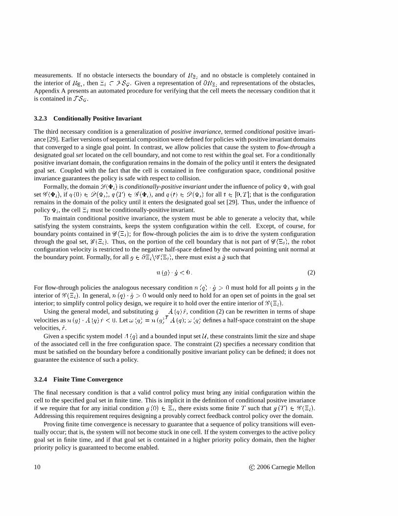
The third necessary condition is a generalization ofpositive invariance, termedconditionalpositive invari-ance [29]. Earlier versions of sequential composition weredefined for policies with positive invariant domainsthat converged to a single goal point. In contrast, we allow policies that cause the system toflow-throughadesignated goalsetlocated on the cell boundary, and not come to rest within the goal set. For a conditionallypositive invariant domain, the configuration remains in thedomain of the policy until it enters the designatedgoal set. Coupled with the fact that the cell is contained in free configuration space, conditional positiveinvariance guarantees the policy is safe with respect to collision.

Formally, the domainD(�i) is conditionally-positive invariantunder the influence of policy�i with goalsetG (�i), if q (0) 2 D(�i), q (T ) 2 G (�i), andq (t) 2 D(�i) for all t 2 [0; T ]; that is the configurationremains in the domain of the policy until it enters the designated goal set [29]. Thus, under the influence ofpolicy�i, the cell�i must be conditionally-positive invariant.

To maintain conditional positive invariance, the system must be able to generate a velocity that, whilesatisfying the system constraints, keeps the system configuration within the cell. Except, of course, forboundary points contained inG (�i); for flow-through policies the aim is to drive the system configurationthrough the goal set,G (�i). Thus, on the portion of the cell boundary that is not part ofG (�i), the robotconfiguration velocity is restricted to the negative half-space defined by the outward pointing unit normal atthe boundary point. Formally, for allg 2 @�inG (�i), there must exist a_g such thatn (g) � _g < 0 : (2)

For flow-through policies the analogous necessary condition n (q) � _g > 0 must hold for all pointsg in theinterior ofG (�i). In general,n (q) � _g > 0 would only need to hold for an open set of points in the goal setinterior; to simplify control policy design, we require it to hold over the entire interior ofG (�i).

Using the general model, and substituting_g = A (q) _r, condition (2) can be rewritten in terms of shapevelocities asn (g) �A (q) _r < 0. Let! (q) = n (g)T A (q); ! (q) defines a half-space constraint on the shapevelocities,_r.

Given a specific system modelA (q) and a bounded input setU , these constraints limit the size and shapeof the associated cell in the free configuration space. The constraint (2) specifies a necessary condition thatmust be satisfied on the boundary before a conditionally positive invariant policy can be defined; it does notguarantee the existence of such a policy.

3.2.4 Finite Time Convergence

The final necessary condition is that a valid control policy must bring any initial configuration within thecell to the specified goal set in finite time. This is implicit in the definition of conditional positive invarianceif we require that for any initial conditiong (0) 2 �i, there exists some finiteT such thatg (T ) 2 G (�i).Addressing this requirement requires designing a provablycorrect feedback control policy over the domain.

Proving finite time convergence is necessary to guarantee that a sequence of policy transitions will even-tually occur; that is, the system will not become stuck in onecell. If the system converges to the active policygoal set in finite time, and if that goal set is contained in a higher priority policy domain, then the higherpriority policy is guaranteed to become enabled.


In general, proving finite time convergence for constrainedsystems can be difficult and must be consid-ered for each policy design in conjunction with its cell and goal set specification. Section 4 addresses thisissue for the specific policies used in this paper.

In summary, policies that respect the system constraints, have simple inclusion tests, are completelycontained in the free configuration space, are conditionally positive invariant, and whose vector field flowconverges to a well defined goal set in finite time may be deployed in the proposed hybrid control framework.Together these four requirements mean that the validity of agiven policy can only be evaluated knowing themappingA (q), the associated cell�i, input spaceUi, and the designated goal set. In Section 4, we describe afamily of policies that admit verification of these necessary conditions, and enable deployment of a collectionof valid policies.

3.3 Discrete Planning in Space of Policies

Given finite time convergence and conditional positive invariance, the closed loop behavior of the controlpolicies induces a discrete transition relation between the cell and its associated goal set. If the goal set ofone policy is contained in the domain of another, the discrete transition relation is defined between policies.Recall from Section 2, that these discrete transitions between policies in a collection,�, may be representedby a directed, generally cyclic, graph structure,��. This allows the continuous dynamics to be representedby the more abstract discrete transitions on the graph. Using appropriate discrete planning tools, severalhigh-level planning problems may be addressed using the underlying feedback control policies that inducethe discrete transitions.

This subsection describes an extension to the conventionaldefinition ofprepares, and the impact on theresulting graph structure. The subsection concludes with adiscussion of the pros and cons of some techniquesfor planning in the space of policies associated with the graph.

3.3.1 Extensions to Prepares Definition

Often the size of a valid cell that satisfies the policy requirements is tied to the size of the specified goal set.To enable larger cells, it is useful to consider policies where several policy domains cover the designatedgoal set, but no single policy domain covers the designated goal set. The conventional definition ofprepares,�j � �i if G (�j) � D(�i), describes a relation between two policies [11]. We extend this definition to arelation between a policy and a set of policies. A selected policy, �i, preparesa set of policies if the goalset of the selected policy,G (�i), is contained in the union of the domains of the policies in the set, that is�i � f�jg if G (�i) � Sj D(�j). Consider Figure 6-a, where�H � f�D;�Gg.

Under the influence of a given control policy, the flow along the induced vector field over a given cell ismathematically determinate; however, from the perspective of the discrete transition relation defined by theprepares relationship, the single policy could result in a transition to any of the policies in the union. In otherwords, while it is possible to determine the subset of the given control policy domain that enters a particularpolicy domain in the union, the resulting calculations are complicated. Restricting the domain representationto simple cells introduces indeterminacy into the graph structure��; this indeterminacy can be represented asanactionwith multiple outcomes, as shown in Figure 6-b. From the point-of-view of the discrete transitionsencoded by��, this indeterminacy results in the outcome being imposed asan external choice that a discreteplanner has no control over. Consider the example paths shown as dotted lines in Figure 6-a. The paths startfrom two different initial conditions, denotedÆ and�, and exit the goal set of�H in different locations,thereby entering different policy domains,�D and�G.

Using this extended definition of prepares allows flexibility in instantiating policies that might otherwisenot be deployable using the conventional definition of prepares. This added flexibility comes at the cost ofadded complexity at the planning stage. If the extended definition of prepares is used to deploy policies,


D

G

H A

B

E

C

F

J I

a) Prepares relationship between a collection of policies.

A

B

H

E

C D

G F

J I

b) Graph representation of the induced discrete abstraction.

Figure 6: This figure shows the relation between a set of policies and the discrete abstraction. The goal sets ofthe policies are the right edges of the bounded regions; either the small end of the funnel shapes or the minoraxis of the half-ellipses. In this example,�H preparesf�D;�Gg. Note, that different initial conditions(denotedÆ and�) in �H lead to different paths through the policy graph.

then the discrete planner must take this indeterminacy intoaccount. Therefore, the design choice to deploypolicies using this extended definition of prepares must be evaluated given the particular planning problemat hand, the constraints in the specific robot model, the environmental complexity, and the available planningtools.

3.3.2 Planning in Policy Space

The discrete policy graph,��, represents the continuous dynamics of the problem as a finite set of transitionsbetween nodes corresponding to policies. Thus, a fundamentally continuous navigation problem is reducedto a discrete graph search over��. If the current configuration is contained in the domain of a policy corre-sponding to a node in��, and a path through�� to the overall goal node exists, then the given navigationproblem is solvable with the collection of currently instantiated policies. Proving that such a graph traversalexists, and ordering the policies to generate a valid traversal, is the specialty of discrete planners.

To facilitate planning, each edge in�� may be assigned a cost. Any non-negative cost is permitted,but the choice of cost impacts the resultant ordering, and hence the overall behavior of the system. In theexperiments presented in this paper, a heuristic cost is assigned based on the relative complexity of each policyand a measure of distance between policy goal sets. By executing the feedback control policies according toan ordering determined by a discrete planner, the trajectories induced by the local policies solve the specifiednavigation problem. Given policies that meet the above requirements, the proposed technique is amenable toany number of discrete planning tools.

The most basic discrete planning approach is to order the policies in the graph according to the assignedcosts [11]. First, a node in the graph is identified as the overall goal node; that is the node corresponding tothe policy that flows to the overall goal set. From this goal node, basic graph search techniques may be usedto order the graph and build the partial order�0�; that is, convert the generally cyclic graph�� into an acyclictree�0�. Dijkstra’s Algorithm, A*, or D*, are natural candidates for this planning [12].

Given the ordered graph,�0�, there are two basic approaches to executing the policies. The simplest isto convert�0� into a total ordering of the policies [11]. Given the currentstate of the system, the hybridcontrol strategy searches for the highest priority policy whose domain contains the current state and executesthat policy. This is simple to implement, and allows the hybrid control system to opportunistically switch toa higher priority policy. The drawback to this approach is that significant search time relative to real timeoperation may be required for large graphs; this approach makes having efficient inclusion tests imperative.


Another approach is to use use the local structure of the tree�0� to guide the search for an active pol-icy. This introduces an internal state where the system mustkeep track of the previously active policy, butallows the system to search a limited number of successors ofthe previously active policy that are expectedto become active. If no successor is valid, the previously active policy is checked. If neither a policy corre-sponding to a successor in the tree nor the previously activepolicy is valid due to some system perturbation,then the hybrid control system can resort to searching the tree as a total order based on the node cost usedduring construction of the tree. This approach will typically require fewer policy domain inclusion tests, butlimits the chance for opportunistic policy switching.

While the choice of switching strategy impacts the induced system trajectory, the convergence guaranteesof the hybrid system are maintained so long as the graph ordering is observed. This inherent flexibility inthe hybrid system approach may be exploited by a high-level planner by selecting a switching strategy forchoosing between valid policies before the system execution, or possibly by using higher-level informationto change the switching strategy on-the-fly. This later possibility is beyond the scope of this current work,but is allowed by the hybrid control framework.

Once the initial ordering is generated, the discrete representation allows for fast re-planning in the event ofchanging conditions. The D* algorithm and its variants are expressly designed to allow for existing plans tobe modified if the cost structure is updated [39, 52]. For example, consider an ordering that uses a policy thatnavigates a particular doorway. If the doorway is unexpectedly closed, the robot may use this new informationto update the graph cost structure – thereby invalidating the policy that passes through the doorway – andreorder the remaining policies. By operating on the discrete policy-based graph, which will generally havefewer nodes than a conventional grid-based path planning graph, the policy-based re-planning step is fasterthan conventional grid-based re-planning, while preserving the guarantees of feedback policies.

One of the key benefits to planning using the ordered graph�0� is the inherent robustness. If an externaldisturbance invalidates a currently active policy, the system can quickly search the ordering for another validpolicy. Consider the case shown in Figure 7, which is a close up of the layout in Figure 6. For the path shown,the system begins executing�G then�F ; during execution of�F an external disturbance moves the stateoutsideD(�F ). By searching the ordered graph,�J may be activated without needing to stop and replan.This allows the system to plan once, and execute many times; in contrast to conventional approaches, thatmust completely re-plan the desired paths in response to significant perturbations.

The biggest drawback to the ordering approach is that only one navigation task at a time can be addressed.This works well for simple navigation tasks, but does not allow for higher level task specifications that requiremultiple goals. Recent work has addressed this issue by combining the policy graph�� with temporal logicspecifications [19, 20]. The approach uses model checking techniques to generate an open loop sequence of

G E F

J I

perturbation

Figure 7: An ordering of policies provides robustness to external disturbances. When an external disturbancemoves the state outsideD(�F ), �J is activated without needing to stop and replan.


policies that satisfy the temporal logic specification. This approach works well for specifying multiple goals,but loses the robustness inherent in the partial order approach.


4 Local Policy Definitions

In defining the local policies, there are several competing goals. First, we desire policies with simple repre-sentations that are easy to parameterize. Additionally, wedesire policies that have simple tests for inclusionso that the system can determine when a particular policy maybe safely used. On the other hand, for a givenpolicy goal set, we want the policy domain to capture as much of the free configuration space as possiblegiven the system constraints. That is, we want the policies to beexpressive. This paper considers how far aset of relatively simple policy parameterizations can be pushed.

To simplify the control policy design problem, the remainder of this paper is limited a particularly simpleclass of robots. First, the mappingA (q) is only a function of the orientation of the robot body; that isA (q) = A (g) = A (�). Second, the robot dynamics are kinematic; that is, the robot directly controlsthe shape variable velocities_r = u for inputsu 2 U . These two restrictions allow the shape variables tobe ignored, and thusq = g. Differential-drive robots, which are widely used, are in this class of robotsprovided their inputs are considered kinematic. This paperwill focus on a specific robot model that meetsthese restrictions – thekinematic unicycle[12, 35]. The kinematic unicycle uses inputs that control ofthe

forward speed,v, and rate of body rotation,!. Given,u = �v !�T 2 U � IR2, the body position andorientation velocity is_g = A (g)u, whereA (g) = 24cos � 0sin � 00 135 : (3)

The mappingA (g), which is defined by the control vector fields that annihilatethe nonholonomic constraints,is fundamental to the policy design techniques developed inthis section.

This section develops a class of generic policies based on a parameterized representation of the cellboundary. First, the basic cell definitions are presented. Given the cell definition, the four requirements fromSection 3.2 are verified. As part of this verification, we use the mappingA (g) to generate a vector fieldthat satisfies the policy requirements and maps a configuration in the cell to a specific control input,u. Theresulting closed-loop dynamics naturally satisfy the nonholonomic constraints inherent inA (g).

The cells,�i, represent a set of configurations in the configuration spaceG. The cells are defined in anIR3 representation ofG relative to a world coordinate frame withfx; y; �g-coordinate axes . We choose todefine generic cells relative to a local coordinate frame attached to the center of the cell’s designated goal set;let ggoal denote the goal set center in the world frame andfx0; y0; �0g denote the coordinate axes of the localreference frame.

Given a generic cell specified in the local coordinate frame,the cell is instantiated in the configurationspace by specifying the location ofggoal and the orientation of the local frame relative to the world frame. Werestrict the policy goal set to lie within a plane orthogonalto the world framex-y plane; thus the local�0-axisis parallel to the world�-axis. We restrict the positivex0-axis, which corresponds to the goal set normal, to bealigned with the robot direction of travel at the configuration corresponding toggoal. Thus, the localx0-axisis normal to the cell goal set, and outward pointing with respect to the cell boundary. Let�goal specify theorientation of thex0-axis, and letggoal = fxgoal; ygoal; �goal +��g 2 IR3. For forward motion, thex0-axisis aligned with the robot heading, and�� = 0. For reverse motion, thex0-axis is opposite the robot heading,therefore�� = ��.

The remainder of this subsection describes the definition ofthe cells relative to this local cell frame. Thatis, a parameterization ofp = fx0; y0; �0g is given. Given the goal set centerggoal, any pointp 2 fx0; y0; �0grepresented in the local generic cell frame can be mapped to apointg 2 G byg (p) = 24cos �goal � sin �goal 0sin �goal cos �goal 00 0 135 p+ 24 xgoalygoal�goal +��35 : (4)


Although similar to a homogeneous transform, the non-standard transformation (4) is required due to theplacement of the cell withinIR3. The cell is both positioned and rotated by�goal; �� is used to position thecell along the�-axis, but does not affect the orientation of the cell.

To define the generic cells, a good definition of the cell’s designated goal set is needed, along with aspecification of the cell boundary. In keeping with sequential composition, the general idea is to “funnel”relatively large regions ofG into the cell’s goal set. This is analogous to the fan-shapedregions of workspacedefined by the optimal paths of car-like systems [56]. Therefore, we chose to define the cells such that theyfan out from the goal set using a generalization of a superquadric surface [26].

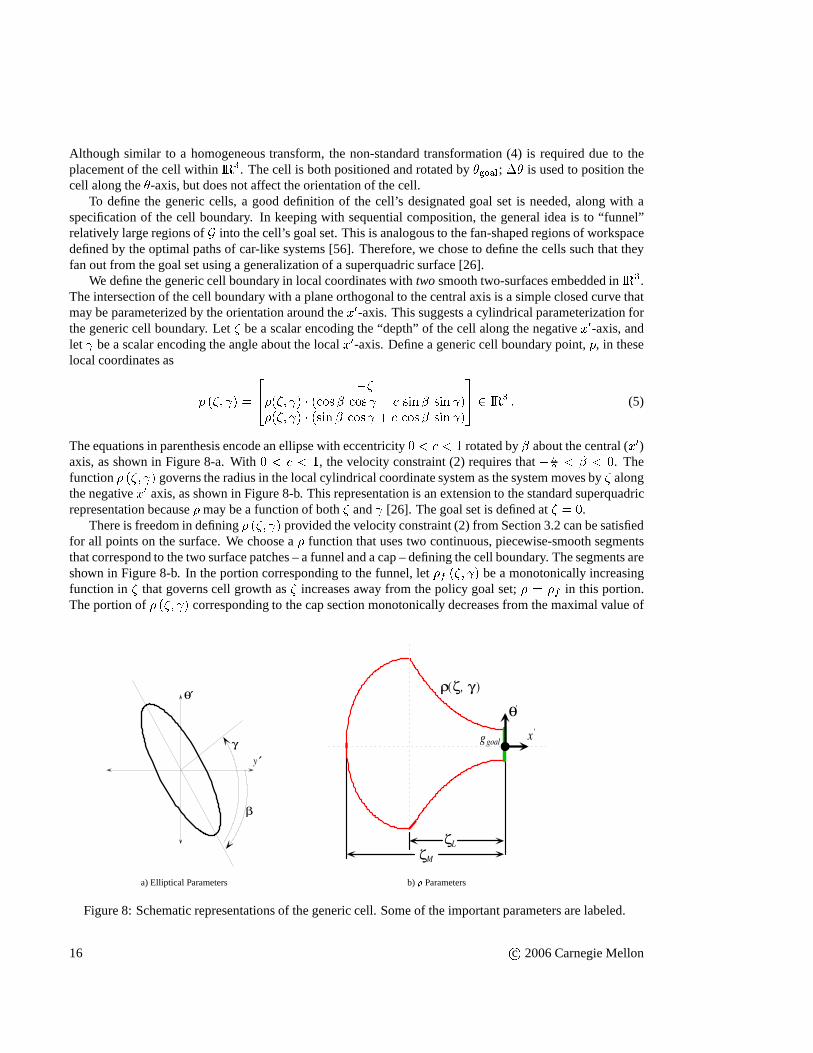
We define the generic cell boundary in local coordinates withtwosmooth two-surfaces embedded inIR3.The intersection of the cell boundary with a plane orthogonal to the central axis is a simple closed curve thatmay be parameterized by the orientation around thex0-axis. This suggests a cylindrical parameterization forthe generic cell boundary. Let� be a scalar encoding the “depth” of the cell along the negativex0-axis, andlet be a scalar encoding the angle about the localx0-axis. Define a generic cell boundary point,p, in theselocal coordinates as p (�; ) = 24 ��(�; ) � (cos� cos � c sin� sin )�(�; ) � (sin� cos + c cos� sin )35 2 IR3 : (5)

The equations in parenthesis encode an ellipse with eccentricity 0 < c < 1 rotated by� about the central (x0)axis, as shown in Figure 8-a. With0 < c < 1, the velocity constraint (2) requires that��2 < � < 0. Thefunction� (�; ) governs the radius in the local cylindrical coordinate system as the system moves by� alongthe negativex0 axis, as shown in Figure 8-b. This representation is an extension to the standard superquadricrepresentation because� may be a function of both� and [26]. The goal set is defined at� = 0.

There is freedom in defining� (�; ) provided the velocity constraint (2) from Section 3.2 can besatisfiedfor all points on the surface. We choose a� function that uses two continuous, piecewise-smooth segmentsthat correspond to the two surface patches – a funnel and a cap– defining the cell boundary. The segments areshown in Figure 8-b. In the portion corresponding to the funnel, let�f (�; ) be a monotonically increasingfunction in� that governs cell growth as� increases away from the policy goal set;� = �f in this portion.The portion of� (�; ) corresponding to the cap section monotonically decreases from the maximal value of

β

θ ′

y ′

γ

a) Elliptical Parameters

g goal

ζ M

ζ L

θ '

x '

ρ ( ζ , γ )

b) � Parameters

Figure 8: Schematic representations of the generic cell. Some of the important parameters are labeled.


�f to zero at the maximal extent of�. Formally, define the complete function as� (�; ) = ( �f (�; ) 0 < � � �L�f (�L; ) p(�M��L)2�(��L)2�M��L �L < � � �M : (6)

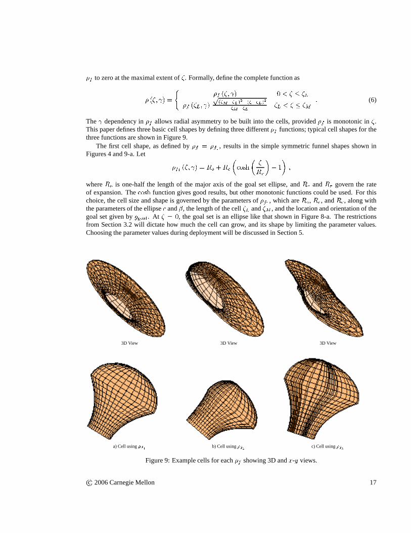
The dependency in�f allows radial asymmetry to be built into the cells, provided�f is monotonic in�.This paper defines three basic cell shapes by defining three different�f functions; typical cell shapes for thethree functions are shown in Figure 9.

The first cell shape, as defined by�f = �f1 , results in the simple symmetric funnel shapes shown inFigures 4 and 9-a. Let �f1 (�; ) = Ro +Re�cosh� �Rr�� 1� ;whereRo is one-half the length of the major axis of the goal set ellipse, andRe andRr govern the rateof expansion. Thecosh function gives good results, but other monotonic functionscould be used. For thischoice, the cell size and shape is governed by the parametersof �f1 , which areRo, Re, andRr, along withthe parameters of the ellipsec and�, the length of the cell�L and�M , and the location and orientation of thegoal set given byggoal. At � = 0, the goal set is an ellipse like that shown in Figure 8-a. The restrictionsfrom Section 3.2 will dictate how much the cell can grow, and its shape by limiting the parameter values.Choosing the parameter values during deployment will be discussed in Section 5.

3D View 3D View 3D View

a) Cell using�f1 b) Cell using�f2 c) Cell using�f3Figure 9: Example cells for each�f showing 3D andx-y views.


The second cell shape, as defined by�f = �f2 , is used to generate a one-sided asymmetric cell, as shownin Figure 9-b. Let �f2 (�; ) = Ro +Re �cosh� �Rr�� 1� � 1 + cos ( � a)2 ;whereRo, Re, andRr are as defined above, and a is used to localize the asymmetry relative to the angleabout the central axis. As with the first function, the goal set at � = 0 is an ellipse.

The third cell shape, as defined by�f = �f3 , is used to generate a two-sided asymmetric cell, as shownin Figure 9-c. This cell is designed to generate a more aggressive turn than the first two cells allow undercondition (2). Let �f3 (�; ) = �Ro +Re�cosh� �Rr�� 1�� 1 +Kg1 exp � (cos ( � g1)� 1)2�g1 !+ Kg2 exp � (cos ( � g2)� 1)2�g2 !! ;whereRo, Re, andRr are as defined above,Kg1 andKg2 specify the relative size for the two wings of thecell,�g1 and�g2 specify the width of the wings, and g1 and g2 localize the wings relative to the angle aboutthe central axis. Unlike the first two functions, the goal setof �f3 is not an ellipse.

Given the classes of generic cells defined by these three functions, it must be shown that instantiations ofthe cells satisfy the necessary conditions given in Section3.2.

4.1 Inclusion Test

Given a cell, the system must check if the current robot position and orientationg 2 G is inside the cell. Theinclusion test makes use of the cylindrical representationof the cell. Givenq = fg; rg 2 Q and a selectedcell, representg in the local cylindrical coordinate frame of the cell asf�q ; q ; �qg, where�q is the distancefrom ggoal along the central axis, q is the angle relative to the ellipse major axis, and�q is the radial distancefrom the cell’s central axis. Since the cell is defined in anIR3 chart ofSE(2), we must also test for inclusionbased ong = fx; y; � + 2n�g wheren 2 f�1; 0; 1g.

The inclusion test uses two steps. The first step tests that0 < �q < �M ; if �q � 0 or �q � �M then thepoint is outside the cell. If the point passes the first test, then find the cell boundary point,pb = f�q ; q; �bgthat corresponds tog = f�q ; q ; �qg, where�q and q are the same and�b is the radius of the boundary pointalong the vector defined by�q and q. These points are shown in Figure 10. From (5), the value of�b is givenas �b (�q ; q) = ��(�q ; q) � (cos� cos q � c sin� sin q)�(�q ; q) � (sin� cos q + c cos� sin q)� = � (�q ; q)p1 + c2 � (c2 � 1) cos (2 q)p2 : (7)

If �q < �b and0 < �q < �M , the configuration is within the cell.

4.2 Free Configuration Space Test

We verify that the cell is contained in the free space of positions and orientations, that is�i � FSG , usingthe approach outlined in Appendix A. The test is for a specificcell using a particular choice of cell parameter


g goal

θ '

x '

ρ b

ζ q

g

p b

Figure 10: Corresponding boundary points. Given a pointg, determine its local cylindrical coordinates,f�q ; q; �qg, and find the corresponding pointpb = f�q ; q; �bg on the cell boundary.

values,fRo; Re; Rr; c; �; �L; �Mg and optionallyf ag or fKg1 ; g1 ; �g1 ;Kg2 ; g2 ; �g2g. Using the param-eterized representation of the cell boundary given in (5), the approach described in Appendix A generates arepresentation ofR�i . The setR�i is tested for intersection with any obstacle. If intersection occurs, the cellparameter values must be modified.

From (5), a point on the cell boundary,g (�; ) = g (p (�; )), and surface normal,n (�; ) = D�g�D gkD�g�D gk ,

can be calculated for the given set cell parameter values. Both g (�; ) andn (�; ) are piecewise smoothfunctions. Given an implicit representation of the robot body boundary, the cell boundary point is analyticallymapped to a point inR�i . By determining points along the boundary ofR�i , intersection with obstacles canbe tested.

Appendix A describes an approach based on a triangulation ofthef�; g parameter space that leads toa projection of the triangulated surface into the workspace. For the deployment presented in this paper, asurface visualization tool was used to visually inspect theprojection for intersection with an obstacle; thisis shown in Figure 5. Future work will automate this test by using the brute force method described inAppendix A.

4.3 Conditional Invariance Test

During instantiation, the cell parameter values must be selected so that the control system can generatevelocities that enforce conditional positive invariance as described in Section 3.2.3. For the models used inthis paper, where_g = A (g)u, condition (2) can be rewritten asn (g (�; ))T A (g (�; ))u < 0 :This condition must hold over the entire cell boundary,@�i. LetU be the bounded input set associated withthis policy, for each pointg (�; ) 2 @�i defineL (�; ) = minu2U n (�; )T A (g (�; ))u : (8)

For a valid cell, condition (2) must hold, such thatL (�; ) < 0 over the entire cell boundary. In other words,at each point on the cell boundary, the system must be able to generate a velocity that is inward pointing withrespect to the cell boundary. Thus, in the worst case over theboundary, a valid cell satisfies the constraintmax�; L (�; ) < 0 : (9)


02

4

−20

2

−0.4

−0.2

0

ζγ

L

Figure 11: Constraint surface forL (�; ) from (8).

Although non-linear, the functionL (�; ) is piecewise smooth and generally “well-behaved” for themappingA (g); therefore, it is feasible to verify that (9) is satisfied fora given set of cell parameter values.Figure 11 shows a typical constraint surface for the cell shown in Figure 4. The ridges shown in the figureare due to switching behavior in the minimization that occurs when the cell boundary normal is parallel tothex-y plane; that is the component in the� direction is zero.

If condition (9) is satisfied for a given cell, then it is possible to define a control law over that cell thatenforces conditional positive invariance. Designing sucha control law, and proving that it provides finite timeconvergence to the cell goal set, is the next topic.

4.4 Vector Field Definition and Convergence Test

To define the control law, we use a family of level sets based onthe cell boundary parameterization givenin (5). This family of level sets is used to define a control vector field that flows to the policy goal set.For g 2 �i, the corresponding level set that passes throughg must be determined; representg in the localcylindrical representation of�i by f�q ; q; �qg.

Recast the cell definition equations given in (5) and (6) in terms of� 0M and� 0L to differentiate the controllevel sets from the cell boundary. These parameters controlthe relative length and size of the internal levelset. Asg 2 �i, the values will have the following relationship0 � � 0L � �q � � 0M � �M . The family of levelsets used for control are defined by (5) with� (�q ; q) = �L (�q ; q) where�L (�q ; q) = �f (� 0L; q) q(� 0M ;�� 0L; )2 � (�q � � 0L; )2� 0M ;�� 0L; : (10)

That is, the control level set is governed the by (6), with�f (� 0L; q) using the same parameter values as thosedefining the cell boundary.

First consider the case� 0M ;= 0 and� 0L;= 0, the level set defined by�q = 0 and q 2 (��; �] correspondsto the policy goal set. Increasing� 0M , while fixing � 0L = 0, generates a family of level sets for0 � �q � � 0Mthat grow out from the goal; these are termed theinner level sets, as shown in Figure 12. By fixing� 0M at itsmaximum value,� 0M = �M , and increasing� 0L, theouter family of level sets grows; these are also shown in


Outer level sets

Inner level sets

g

ζ L '

ζ q

Figure 12: Level Set Definition for control

Figure 12. Thus, giveng = f�q ; q; �qg, the values for� 0M and� 0L must be determined such that the level setpasses throughg. For this to be the case,�L (�q ; q) = �q; thus values for� 0M and� 0L that satisfy�f (� 0L; q) q(� 0M � � 0L)2 � (�q � � 0L)2� 0M � � 0L � �q = 0 (11)

must be found.For configurations within the inner family of level sets,� 0L = 0 and� 0M can be determined in closed-form

from (11). If the configuration is within the outer family of level sets, as shown in Figure 12, then� 0M = �Mand we must determine the value of� 0L that satisfies (11). Unfortunately,� 0L cannot be found in closed form.Fortunately, (11) is a monotonic function of� 0L, which admits a simple numeric root finding procedure.

Given the values of� 0M and� 0L, the level set normal is used to define a constrained optimization over theinput space. The level set normaln (�q ; q) is defined as in Section 4.2 using (5) and (10). The simplestconstrained optimization isu� = argminu2U [n (�q ; q) � A (g (�q ; q))u] s:t: n (�q ; q) �A (g (�q ; q))u < 0: (12)

For a convex polygonal input setU , the solution to this optimization will lie at the vertices of U . To smoothu�, the cost function,[n (�q ; q) � A (g (�q ; q))u], can be augmented by a simple quadratic term.Using u� as the control input drives the system from the outer level sets to the inner level sets, and

then continuously on to the goal. We force all the inner and outer level sets to satisfy (9) at every pointin the cell, which guarantees that a solution to (12) exists.The body velocity_g = A (g)u� will bring thesystem configuration to a “more inward” level set; thus, the system moves a finite distance closer to the goal.Although a formal analytic proof is lacking, experience shows that if the outermost level set correspondingto the cell boundary satisfies (9), all interior level sets will also satisfy (9). This can be checked for variousvalues of�M and�L during deployment.

Given the inputu�, the reference vector field over the cell�i is simplyA (g)u�. In reality, onlyu� isimportant; the vector field is induced by the flow of the systemgiven the control inputs, and is never explicitlycalculated.


5 Policy Deployment Technique

To deploy a policy in this sequential composition framework, we must specify the parameters that governthe location, size, and shape of the cell. Given a specification of these parameters, the requirements fromSection 3.2 must be verified. Currently, we lack an automatedprocess for deploying the policies; therefore,we use a manual, trial and error, process to specify the policy parameters. Future work will develop automateddeployment methods. While there are many possible deployment approaches, this section focuses on theapproach used in the experiments described in Section 6.

The policies are generally deployed sequentially using a backchaining procedure; that is, we test theprepares relationship to ensure the policies prepare at least one policy. We begin instantiating a policy byspecifying that the policy goal set is completely containedwithin the domain of a set of existing policies.Assume at least one safe policy is instantiated; that is, initially � = f�0g where�0 stops the system in asafe configuration.

For the policies presented here, the prepares test can be done by verifying that all points on the policygoal set boundary are contained in the domains of neighboring cells. First, we specifyggoal to lie within thedomain of an existing cell, or set of cells; this is verified automatically using (7). Next, we initialize the policygoal set by specifying the elliptical parameters� andc from (5) and the function� (0; ) by specifying theparameters in�f . We test that the policy goal set boundary does not intersectthe boundary of the neighboringcell, or the boundary of the union of neighboring cells. For this test we use a automated test based on (7) for adense sampling of points around the goal set boundary. The check can also be done visually using Figure 13.We iteratively adjust the parameters, including the policygoal set centerggoal, as needed until the policy goalset is fully contained in the neighboring cell or set of cells. During this iterative process, we also test that thepolicy goal set is valid with respect to the mappingA (g) and chosen input set; that isming2G(�i)maxu2U n (g)T A (g)u > 0 :For g 2 G (�i), n (g) is aligned with the localx0-axis. Assuming that the previously deployed policies arecontained in free configuration space, a valid goal set will lie inFSG.

If the goal set is not contained in a single policy, a simplified version of the extended prepares test(�j � f�ig) is used to test for inclusion in the union of neighboring policy domains. Here, we requirethat each neighboring policy in the union contain the goal center of the policy being tested. This is shownin Figure 14, where the goal center for�D is contained in the cells labeledA, B, andC. Then, for each

J

I

a) Schematic view of prepares test b) Prepares test in 3D c) Prepares test in 3D - close up

Figure 13: Prepares test for policy deployment. In the 3D figures, the goal set of�J and the correspondingpoints on the surface of�i are traced in lighter colors.


θ ′

C

B

A

D

Figure 14: Prepares test for union of policy domains. Here�D � f�A;�B ;�Cg.point on the goal boundary of�j , the maximum of the minimum distance to the cell boundaries is found.For all 2 [��; �] find gj (0; ), a point on the goal set boundary of�j in the world frame. For each�ifind �qi (gj (0; )), qi (gj (0; )), and�qi (gj (0; )) ; then, using (7) find�bi (�qi (gj (0; )) ; qi (gj (0; ))).The goal set prepares the union of neighboring cells ifmin maxf�ig ��bi ��qi (gj (0; )) ; qi (gj (0; ))� �qj (�qi (gj (0; )) ; qi (gj (0; )))�� > 0 :This test is performed automatically based on a dense sampling of points around the the goal set boundary;the result can also be checked visually as in Figure 13.

Given a valid policy goal set, we grow the cell by specifying the parameters that determine the rate ofcell expansion and cell shape, includingRe, Rr, �L and�M . During this process, we must confirm that (9)is satisfied and that the cell remains in the free configuration space. Given these conditions, the requirementsthat we can reach the goal in finite time and have a test for cellinclusion are automatically satisfied given themethods for defining the cell and vector field.

The test that (9) is satisfied is automated by using numericaloptimization to find the maximum value of(8) over thef�; g parameter space. Given a violation of (9), we iteratively adjust the parameters as neededto ensure the requirements are met. Figure 11 can be used to guide the process of modifying parameters byshowing where the violation occurs on the cell boundary.

To verify that a policy is safe with respect to obstacles, we use the expanded cell described in Section 3.2.In these experiments, we graphically verify that the projection of the expanded cell is free of intersection. Wesample thef�; g parameter space with a fine resolution mesh, and calculate the corresponding points on theexpanded cell surface. We project the resulting expanded cell surface mesh into the workspace and visuallycheck for obstacle intersection, as shown in Figure 22-b. Ifcollision occurs, the parameters governing cellsize and shape are adjusted as needed, and both the free spaceand (8) tests are repeated.

Once an instantiated policy has been validated, it may be added to the collection of instantiated policies,�.


Given a collection of instantiated policies, the final step is to specify the prepares graph,��; this step iscompletely automated. The automated graph builder checks the prepares relationship for each policy againstall other policies in the deployment; that is we test for policy goal set inclusion within other cells or sets ofcells as described above. For the deployment used in this paper, collections of up to three cells were testedfor the extended prepares. For policies that have a preparesrelationship, we assign an edge cost heuristicallybased on the path length between the goal center and the prepared cells associated goal center, and a factor forthe policies relative complexity. By assigning a relatively high transition cost between forward and reversepolicies, changes in direction are reduced.

Currently, the trial and error process of policy instantiation takes between two and 30 minutes. The timedepends mainly on the tightness of the corridors and sharpness of the turns being navigated. The final graphgeneration step is fully automated; it took several hours torun for the collection of 271 policies Section 6.The up-front cost of generating the deployment is mitigatedby the ability to reuse the policies by planningmultiple scenarios on the discrete graph.


6 Current Results

The control techniques and cells described in this paper have been validated experimentally on a real mobilerobot. This section describes the robot system used to validate the work, and describes the deployment ofpolicies used in the experiments. Several navigation experiments on the physical robot are discussed. Theseexperiments demonstrate planning and re-planning in the space of deployed control policies. The sectionconcludes with simulation results of planning using temporal logic specifications and model checking toaddress multiple task scenarios.

6.1 Robot System and Implementation

The techniques described in Sections 3 and 4 have been validated on our laboratory robot. This standarddifferential-drive robot, shown in Figure 15, has a convex,roughly elliptical body shape. To simplify cal-culations ofR�i , the composite set of points occupied by the robot body over all positions and orientationsin the cell, the robot body and wheels were tightly approximated by an analytic ellipse centered in the bodycoordinate frame. This is shown in Figure 16. The length of the major and minor axes of the bounding ellipseare1:12 and0:68 meters respectively.

The control policies use the kinematic unicycle model, withthe standard formA (q) = 24cos � 0sin � 00 135 :The inputsu = �v !�T are forward velocity,v, in meters per second, and turning rate,!, in radians persecond.

The policies in the deployment are instantiated by choosingamong a collection of four different inputsets to account for local conditions. The system changes direction by switching between “Forward” and“Reverse” input sets; each having an “Aggressive” and “Cautious” set of values. The numerical values,shown in Figure 17, are based on the velocity limits of the motors, and scaled back for cautious modes andthe reverse input sets. Although the robot is capable of zero-radius turns, the input bounds are chosen tomodel a conventional car-like system with bounded steering. This choice limits the rate of expansion of thecells based on the conditional invariance condition given in (9); the cell shapes would only be limited by theobstacles if zero-radius turns were allowed. This paper uses convex polygonal bounds on each input set; this

Figure 15: Laboratory robot

−0.5 0 0.5−0.5

0

0.5

x (meters)

y (m

eter

s)

Figure 16: Bounding ellipse


−0.4−0.2 0 0.2 0.4 0.6

−0.4

−0.2

0

0.2

0.4

v (m/s)

ω (

radi

ans/

s)

Figure 17: Four sets of bounded steering inputs. Forward Aggressive - , Forward Cautious -}, ReverseAggressive -2, Reverse Cautious -�restriction is for computational convenience, and is not fundamental. Each cell is evaluated with respect to aspecific choice of input set.

For these experiments, a set of polygonal obstacles defines the 10 meter�10 meter world shown inFigure 18-a. The world includes several narrow corridors and openings. The width of the narrow corridorsis approximately one meter. This provides a clearance of approximately 16 centimeters on either side, butprevents the robot from turning around within the corridor.

For these experiments, a total of 271 basic policies of the type described in Section 4 are deployed usingthe techniques described in Section 5. A partial deploymentis shown in Figure 18. Each policy is associatedwith a specific input set from Figure 17. From the collection of instantiated policies,�, the discrete graphrepresentation,��, is determined. The deployment uses the extended definitionof prepares described inSection 3.3.1, so that 15 separate policies prepare 31 different unions of policy domains.

a) Projection of cells into workspace with obstacles b) Representation of cells in 3D C-space

Figure 18: Partial deployment of cells in environment.


6.2 Navigation Experiments

Given an implementation of the policy deployment and graph structure on the robot, the navigation task isspecified as bringing the robot to a designated goal set located in the middle of the lower corridor. Thedesignated goal set is associated with a specific policy, andtherefore, a specific node in the policy graph.This node is specified as the overall goal of these experiments. An ordering of the policy graph from thisoverall goal node is generated using a Mini-max version of D*Lite [39].

D* Lite [39] resolves the indeterminacy described in Section 3.3.1, and provides an efficient way to re-plan in the case where a policy status is changed to invalid after the initial planning stage. Initially, the plannergenerates a partial order,�0�, of the policy graph�� by assigning a cumulative node cost based on the edgecosts determined during graph generation. If a valid path through the ordered graph from a given policy nodeto the designated goal node does not exist, then the node (andcorresponding policy) is flagged as invalid. Asthe planner executes, the effects of invalid nodes propagate through the graph; as a result, a path to the goalfrom a given node is guaranteed to exist if the node remains valid.

During execution, the hybrid policy tests the current estimate of body position and orientation for in-clusion in the cells associated with successors of the currently active policy. If the current configuration isincluded in one of the successor domains, the associated policy is activated. If not, the currently active policyis checked for validity, and executed if it is still valid. Asa final check if this fails, the robot is temporar-ily stopped and�0� is searched for a valid policy. If this final search fails to find a valid policy, the robotterminates execution and reports failure.

The policy switching is completely automatic once the initial start command is given. The system stopswhen it reaches the policy designated as the goal or, if the configuration is not contained within a valid policydomain. If a valid policy is found, the control is calculatedas described in Section 4.4. On our robot, theforward velocity and turning rate calculated by the controlpolicy is converted to wheel speeds used by thelow-level PID motor control loop.

Seven representative tests on the robot are presented; a total of 19 tests were conducted, all in the sameenvironment. The actual data was logged every 0.1 seconds during the robot experiment, and is plotted withthe obstacles shown in the figures. On the plots, the robot symbols are shown every five seconds of traveltime. Although the policies were initially validated in simulation, the results presented here are for actualrobot runs.

For the experiments described in this paper, the robot lacksan external localization system, thereforethe configuration estimates are based on pure dead-reckoning. As a result of dead-reckoning error, inherentin all wheeled-mobile robots, the robot would have crashed into some obstacles had they been physicallypresent. Therefore, we run the robot in an open space, but usethe policies that consider the obstacles shownin Figure 18-a.

Figure 19-a shows the results of four of the robot runs from four different initial conditions and the samegoal node. To emphasize, the paths shown are plotted from dead-reckoned estimates of body position andorientation from an actual robot run. The induced paths are the result of policy ordering that is based onassigned edge costs in the discrete graph; an explicit desired path is never calculated. The paths are labeled(#1 - 4) clockwise from the lower left.

The path labeled #5, shown in Figure 19-b, begins near the same position as for path #1 (shown in Fig-ure 19-a); however, the orientation is approximately 180 degrees different. As the deployment also includespolicies that allow the robot to go in reverse, the robot backs up, stops, and then moves forward to the goal.To avoid damaging the real robot, the system was required to come to a stop before switching between aforward and reverse policy. The policy switching is automatic, with no operator intervention.

Paths #6 and #7, shown in Figure 20, have two features that demonstrate the flexibility of the approach.First, like path #5, they demonstrate automatic forward/reverse switching. In this case, the deployment doesnot include policies that are expressive enough to turn the lower right corner in one continuous motion. Therobot initiates a K-turn, again with the policy switching occurring automatically as dictated by the policy


a) Experimental Runs #1-4 b) Experimental Run #5

Figure 19: Experimental results of five robot runs using the proposed hybrid control framework. The exper-imental runs use the same ordering determined by a discrete planner, only the initial conditions vary. Theprojection of the individual policy domains are shown in light gray. Runs #1 and #5 start at the same position,but 180 degrees apart in orientation. Run #5 automatically backs out of the narrow corridor, and then switchesto forward motion.

ordering. While this points to the need for future research in designing more expressive policies, it alsovalidates the basic approach as the combination of simple policies with discrete planning is still capable ofgenerating expressive motions.

The second feature demonstrated by paths #6 and #7 is that of re-planning in the discrete space of availablepolicies. The robot starts from slightly different initialconditions, but begins to converge to the same vectorfield flow near the K-turn. Just after the K-turn during run #7,the two policies crossing the circular obstacleshown in Figure 20-b are flagged as invalid. This triggers a re-planning step using D* Lite that reorders thepolicies, thereby inducing the robot to take “the long way around” via path #7. This re-planning occurred inreal time, while the hybrid control policy was executing on the robot.

6.3 Task Level Planning Simulations

To demonstrate the utility of planning in the space of control policies, a multiple task scenario is simulatedusing the same robot model, obstacle environment, and policy deployment described above. The scenariois modeled on a mail delivery robot operating in an office environment. The robot, which begins in a givenregion, is tasked with picking up a package at a designated region, and dropping the package off at the mail-room. The robot is also tasked with picking up two packages atthe mail-room, and delivering them to twoseparate locations. The robot is to finish at a designated region.

Each pickup or delivery point is associated with the goal setof a specific policy. Using the labeling ofpolicies in the deployment, the specification may be given as� Start in location BT� Pickup (visit) at either DE or FO, then deliver to GO (mail-room)


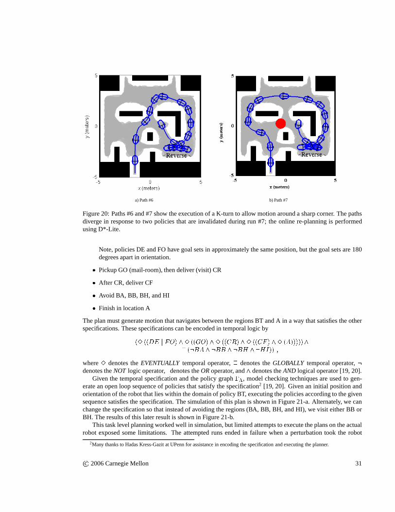
a) Path #6 b) Path #7

Figure 20: Paths #6 and #7 show the execution of a K-turn to allow motion around a sharp corner. The pathsdiverge in response to two policies that are invalidated during run #7; the online re-planning is performedusing D*-Lite.

Note, policies DE and FO have goal sets in approximately the same position, but the goal sets are 180degrees apart in orientation.� Pickup GO (mail-room), then deliver (visit) CR� After CR, deliver CF� Avoid BA, BB, BH, and HI� Finish in location A

The plan must generate motion that navigates between the regions BT and A in a way that satisfies the otherspecifications. These specifications can be encoded in temporal logic by(3 ((DE j FO) ^3 ((GO) ^3 ((CR) ^3 ((CF ) ^3 (A)))))^2 (:BA ^ :BB ^ :BH ^ :HI)) ;where3 denotes theEVENTUALLYtemporal operator,2 denotes theGLOBALLY temporal operator,:denotes theNOT logic operator,j denotes theORoperator, and denotes theAND logical operator [19, 20].

Given the temporal specification and the policy graph��, model checking techniques are used to gen-erate an open loop sequence of policies that satisfy the specification2 [19, 20]. Given an initial position andorientation of the robot that lies within the domain of policy BT, executing the policies according to the givensequence satisfies the specification. The simulation of thisplan is shown in Figure 21-a. Alternately, we canchange the specification so that instead of avoiding the regions (BA, BB, BH, and HI), we visit either BB orBH. The results of this later result is shown in Figure 21-b.

This task level planning worked well in simulation, but limited attempts to execute the plans on the actualrobot exposed some limitations. The attempted runs ended infailure when a perturbation took the robot

2Many thanks to Hadas Kress-Gazit at UPenn for assistance in encoding the specification and executing the planner.


−5 0 5−5

0

5

BT

DE

GO

CF

CR

A

BABBBHHI

x (meters)

y (m

eter

s)

a) Path #1

−5 0 5−5

0

5

BT

DE

GO

CF

CR

A

BBBH

x (meters)

y (m

eter

s)

b) Path #2

Figure 21: Simulation of open loop policy sequences derivedfrom temporal logic specifications.

outside the domain of one of the policies in the open loop sequence. This can be addressed by modifying thepolicies to have a larger domain, thereby making it less likely to escape a policy under perturbation, or byrerunning the model checking based planner with the currentconfiguration as the new initial condition [19].Fundamentally, the open-loop sequences lose the robustness inherent in the partial order approach.

One reason for the system being forced through policies withlimited domains is that the current imple-mentation of the planner does not handle the indeterminacy due to the extended prepares; therefore, edgesconnecting unions of policies were removed from the graph. This forced the system through some policieswith limited domains, making the system much more sensitiveto localization disturbances.


7 Conclusion

The results of simulations and actual robot experiments presented in this paper demonstrate the validity of theapproach, and provide a powerful demonstration of the inherent flexibility of planning in the space of controlpolicies. Policies of the type outlined in this paper enablea large class of discrete planners, including thosethat can handle temporal logic specifications, to work with real, non-ideal, convex-bodied systems operatingin real environments. The approach provides consistent results and maintains the provable guarantees ofthe local control policies, while enabling the flexibility to replan in real time. The sequential compositiontechniques advocated in this paper are generally applicable to a wide variety of control policies — beyondthe flow-through policies described in this paper — providedthe basic requirements that we outline are met.

One shortcoming of this set of experiments is the lack of integrated localization, which prevented the robotfrom running in an actual cluttered environment due to the dependence on dead reckoning. As the ultimatesuccess of the strategy depends on accurate estimates of configuration, future experiments will incorporatevision-based localization that allows the system to estimate its configuration based on the position of knownlandmarks. This will allow testing the control strategy with a fully integrated autonomous system operatingamongst physical obstacles.

Another issue that must be addressed is the time required to instantiate the policies. Currently, the trialand error method used to specify the policy parameter valuesis too time consuming. Future work willincorporate improvements to the deployment scheme that allow faster, more automated deployment. Oneof these improvements, automated methods for testing the inclusion in the free configuration space, wasdiscussed in Section 3.2.2. Work remains in developing automated techniques for specifying the policyparameter values.

A major theoretical issue with the approach is the lack of completeness. The work on automating the de-ployment of local policies will address the completeness issue by automatically deploying additional policieson-line if the current configuration is not contained in the current deployment. That said, there are valid rea-son for not seeking to be complete. By not trying to cover “every nook and cranny” of the free configurationspace, the number of policies is kept reasonable . Limiting the size of the discrete planning problem enablesfaster planning in the space of control policies. By allowing for online deployment when new policies areneeded, the benefits of fast planning can be maintained, while addressing the lack of completeness.

Our immediate research plans are to extend the results to more complicated configuration spaces andsystem models. Specifically, the 4-variable Ackermann steered car, where the mappingA (q) 6= A (g).This structural difference, which necessitates a change inthe control laws, is due toA (q) depending on aninternal shape variable that specifies the steering angle. Additionally, more expressive cell definitions will bedeveloped that allow more aggressive maneuvers relative tothe robot capabilities.


Acknowledgments

The first author would like to acknowledge Sarjoun Skaff and Hyungpil Moon for their assistance with therobot experiments, Maxim Likhachev and Dave Ferguson for helpful discussions and D* Lite code, andHadas Kress-Gazit (UPenn) for generating the task level plans.


A Free Space Testing

This appendix presents an approach to determining the composite set of pointsR�i occupied by a robot bodyover all configurations within a cell�i; that is we determine the swept volume ofR (g) over allg 2 �i. Thisenables testing that a given cell is contained in the free space of positions and orientations of the robot body.The approach presented here is complementary to the approach of expanding obstacles; here we expand thecell.

First, identify the body configuration spaceG withW� IR and map the cell�i toW� IR; in an abuse ofnotation, let�i denote the cell inW� IR. The cell�i � W � IR is expanded to account for the extent of therobot body (Figure 22-a), then the expanded cell is projected toW to yieldR�i (Figure 22-b). It is sufficientto show that no obstacles intersect the boundary ofR�i , denoted@R�i , and that no obstacles are completelycontained in the interior ofR�i . The expansion and subsequent tests depend only on the robotbody shape,the collection of obstacles, and the specific cell shape.

Loosely speaking, the expanded cell is found by calculatingthe Minkowski sum3 ofR (g) and�i, denotedR (g)��i. In this case, however,R (g) is a 2D set inW and both�i andR (g)��i live inW� IR. Anothercomplication is thatR (g) varies withg 2 �i. Thus, the Minkowski sum must be calculated based on aplanar slice of the cell at a given orientation� (Figure 23-a) and the robot body oriented at that orientation.We extend the Minkowski sum definition asR (g)� �i = 8<:24xy�35+ 241 00 10 035 p j g = fx; y; �g 2 �i and p 2 R (f0; 0; �g)9=; ; (13)

whereR (f0; 0; �g) represents the set of robot body points at the origin but rotated by�. This extendeddefinition maps the 2D pointp into the 3D spaceW � IR. This continuous mapping is equivalent to thestandard Minkowski sum of a planar slice of�i at constant orientation with the robot at the same orientation(see Figure 23).

3The Minkowski sum is in contrast to the Minkowski difference, which is used to expand obstacles.

a) Cell expanded to represent robot body extent b)R�i - Extent of robot body in workspace

Figure 22: The cell boundary (dark inner surface) may be expanded to account for the non-trivial robotshape. The minimum signed distance from the boundary@R�i to the closest obstacle is the closest approachof the system to an obstacle under the control of the associated policy. Note, the open face of the goal setis not shown. The goal set will be contained within the domainof another policy, so expanding this set isunnecessary.


a) Cell cut at constant orientation

x

y

b) Robot body at cut boundary point

x

y

c) Boundary of extended cell for cut plane

Figure 23: The calculation of the extended surface is based on a planar Minkowski sum. a) Consider cuttingthe cell at constant orientation. b) The robot body is placedalong the boundary of the cell for this constantorientation. The corresponding point on the extended surface is found by matching normals for the planarcell boundary and the robot body. c) The boundary of the extended cell is calculated.

The composite setR�i is found by projecting the boundary ofR (g) � �i into the workspace using thetrivial projection�xy fx; y; �g = fx; yg 2 W . To determine the boundary, use the convolution surface of@R (g) and@�i. For Minkowski sums of two setsA andB, the boundary ofA � B is a subset of theconvolution of the boundaries@A and@B [45, 46, 49]. That is@ (A�B) � @A � @B, where@A � @B = fa+ b j a 2 @A; b 2 @B; s:t: n@A (a) k n@B (b)g (14)

with n@A (a) the boundary normal toA ata andn@B (b) the boundary normal toB at b. If both sets,A andB, are convex, then@ (A�B) = @A � @B.The convolution surface definition in (14) is extended analogous to the Minkowski extension in (13).

Given a robot configuration point on the cell boundary,g 2 @�i, the corresponding outward pointing normal

to the cell boundary,n (g) = �nx ny n��T , is projected to thex-y plane using the trivial projection�xyn (g) = �nx ny�T . Given a pointp 2 @R (f0; 0; �g), letnR (p) denote the outward pointing normal tothe robot body at orientation�. Then, the robot boundary pointsp such thatnR (p) is parallel to�xyn (g) arefound (see Figure 23-b). The convolution surface@R (g)�@�i, which contains the boundary ofR (g)��i �W � IR, is given by@R (g) � @�i = 8<:24xy�35+ 241 00 10 035 p j g = fx; y; �g 2 �i ; p 2 @R (f0; 0; �g) ; s:t: �xyn (g) k nR (p)9=;

(15)For realistic body representations, this will give a finite number of possible points on the expanded surface.For convex robot bodies, this result gives two potential points; the correct choice is the robot boundary pointwhose normal points in the same direction as the cell boundary normal. Thus, given a piecewise analyticrepresentation of the robot body boundary and a parametric representation of the cell boundary, an exactpiecewise parametric representation of the cell/robot convolution surface,@R (g) � @�i, can be determined.While the convolution surface may define some points on the interior of the expanded cell, the convolutionsurface will contain the expanded cell surface.

Example A.0.1 Elliptical Robot Body.


Consider the elliptical robot body shown in Figure 23-b. In the body reference frame, the robotbody boundary is defined by

�prb = fxrb; yrbg 2 IR2 j f�1 (prb) = 0, where the functionf (prb) =pTrbMprb � 1 with M defined as a2� 2 matrix that encodes the elliptical shape.Use the extended convolution operator (15) to find the point on the expanded cell boundary given a point

on the cell boundary. Letg = fx; y; �g 2 @�i � W� IR represent the configuration of the body referencepoint on the cell boundary, and let the cell surface normaln (g) be given. Define the projected unit vectorn� (g) = �xyn(g)k�xyn(g)k . To determine the expanded cell, the pointp = fxp; yp; �g 2 @R (g)�@�i � W�IRthat corresponds tog must be found.

In the body reference frame, the pointp is given byprb = Rot(�)T �xy (p� g) with Rot(�) the2� 2rotation matrix. Letvp = �xy (p� g), and rewrite the body function asf (p) = vTp Rot(�) M Rot(�)T vp � 1 : (16)

The robot boundary normal in the workspace frame is given bynR (p) = 2Rot(�) M Rot(�)T vp :Sincep, and thusnR (p), is unknown, letk represent the unknownknR (p)k. To satisfy the matchingnormal requirement of the convolution surface, equatenR (p) =k andn� (g) and solve forvp as follows:nR (p)k = n� (g)2Rot(�) M Rot(�)T vp = kn� (g)vp = k2 �Rot(�) M Rot(�)T��1 n� (g)vp = k2Rot(�) M�1 Rot(�)T n� (g) :Substitutevp into (16), and solvef (p) = 0 fork = 2qn� (g)T Rot(�) M�1Rot(�)T n� (g) :Substitutingk into the solution forvp yieldsp = g + 241 00 10 035 vp 2 @R (g) � @�i24xpyp� 35 = 24xy�35+ 241 00 10 035 Rot(�) M�1 Rot(�)T n� (g)qn� (g)T Rot(�) M�1Rot(�)T n� (g)Thus, the pointg = fx; y; �g on the cell boundary is mapped to the pointp = fxp; yp; �g on the convolu-tion surface that contains the expanded cell boundary.

To verify that the set does not intersect an obstacle, the boundary@R�i is found, whereR�i = �xy (@R (g) � @�i).Finding@R�i is equivalent to the silhouette extraction problem in computer graphics. Fortunately, there areseveral existing algorithms that may be used to determine the silhouette of@R (g) � @�i [23].

Given a triangulated surface representation of the expanded cell, a common “brute force” approach isto determine the set of edges that contribute to the projection boundary by examining the adjacent facet nor-mals [23]. The resulting finite set of line segments can be tested for intersection with a obstacle boundary edgeor inclusion of an obstacle vertex inside the projection boundary. The minimum distance from a boundaryline segment to an obstacle may also be determined. The complexity of this approach is linear in the number


of edges in the triangulation. While this brute force approach to silhouette extraction is not appropriate forreal-time calculations, it is easy to implement and is suitable for cell validation during policy instantiation.The accuracy of the technique is determined by the accuracy of the surface triangulation; thus, more trianglesimplies more accuracy. Provided the closest approach to an obstacle is greater than the maximum error in thetriangulation approximation, the cell is contained in the free configuration space.


References

[1] A. M. Bloch et al. Nonholonomic Mechanics and Control. Springer, 2003.

[2] Kwok Wai Au and Yangsheng Xu. Path following of a single wheel robot. InIEEE Conference onRobotics and Automation, pages 2925–2930, San Francisco, CA, USA, April 2000.

[3] J. Barraquand and J.C. Latombe. Nonholonomic multibodyrobots: Controllability and motion planningin the presence of obstacles.Algorithmica, 10:121–155, 1993.

[4] Calin Belta, Volkan Iser, and George J. Pappas. Discreteabstractions for robot planning and control inpolygonal environments.IEEE Transactions on Robotics, 21(5):864–874, October 2005.

[5] Michael S. Branicky. Stability of switched hybrid systems. InProceedings of the 33rd Conference onDecision and Control, pages 3498–3503, 1994.

[6] Michael S. Branicky.Studies in Hybrid Systems: Modeling, Analysis, and Control. PhD thesis, MIT,Dept. of Elec. Eng. And Computer Sci., June 1995.

[7] Michael S. Branicky. Multiple lyapunov functions and other analysis tools for switched and hybridsystems.IEEE Transactions on Automatic Control, 43(4):475–482, April 1998.

[8] Michael S. Branicky. Behavioral programming. InWorking Notes AAAI Spring Symp. on HybridSystems and AI, Stanford, CA, March 1999.

[9] Michael S. Branicky and Gang Zhang. Solving hybrid control problems: Level sets and behavioralprogramming. InProc. American Control Conference, pages 1175–1180, Chicago, IL, June 2000.

[10] R. W. Brockett. Asymptotic stability and feedback stabilization. In Roger W. Brockett, Richard S.Millman, and Hector J. Sussmann, editors,Differential Geometric Control Theory, pages 181–191.Birkhauser Boston, 1983.

[11] R. R. Burridge, A. A. Rizzi, and D. E. Koditschek. Sequential composition of dynamically dexterousrobot behaviors.International Journal of Robotics Research, 18(6):534–555, 1999.

[12] Howie Choset, K. M. Lynch, S. Hutchinson, G. Kantor, W. Burgard, L. E. Kavraki, and S. Thrun.Principles of Robot Motion: Theory, Algorithms, and Implementations. MIT Press, 2005.

[13] David C. Conner, Alfred A. Rizzi, and Howie Choset. Composition of Local Potential Functions forGlobal Robot Control and Navigation. InIEEE/RSJ Int’l. Conf. on Intelligent Robots and Systems,pages 3546 – 3551, Las Vegas, NV, October 2003.

[14] C. I. Connolly and R. A. Grupen. Nonholonomic path planning using harmonic functions. TechnicalReport 94-50, UMass Computer Science, 1994.

[15] C. Canudas de Wit and R. Roskam. Path following of a 2-DOFwheeled mobile robot under path andinput torque constraints. InIEEE International Conference on Robotics and Automation, pages 1142 –1146, April 1991.

[16] R. DeCarlo, M. Branicky, S. Pettersson, and B. Lennartson. Perspectives and results on the stabil-ity and stabilizability of hybrid systems.Proceedings of the IEEE, Special Issue on Hybrid Systems,88(7):1069–1082, July 2000.

[17] F. Diaz del Rio, G. Jimenez, J. L. Sevillano, S. Vicente,and A. Civit Balcells. A generalization of pathfollowing for mobile robots.Journal of Robotic Systems, 18(7):325 – 342, 2001.


[18] A. Deluca, G. Oriolo, and C. Samson.Robot Motion Planning and Control, chapter Feedback Controlof a Nonholonomic Car-Like Robot, pages 171–254. Springer-Verlag, 1998.

[19] George Fainekos, Hadas Kress-Gazit, and George J. Pappas. Hybrid controllers for path planning: Atemporal logic approach. InIEEE Conference on Decision and Control, Seville, Spain, 2005.

[20] George Fainekos, Hadas Kress-Gazit, and George J. Pappas. Temporal logic planning for mobile robots.In IEEE Conference on Robotics and Automation, Barcelona, Spain, 2005.

[21] Th. Fraichard. Motion planning for autonomous car-like vehicles. Ercim News (42):26-28, July 2000.

[22] E. Frazzoli, M.A. Dahleh, and E. Feron. Robust hybrid control for autonomous vehicle motion plan-ning. InProceedings of the 39th IEEE Conference on Decision and Control, volume 1, pages 821–826,Sydney, Austrailia, 2000.

[23] Bruce Gooch. Silhouette extraction. InCourse Notes for Theory and Practice of Non-PhotorealisticGraphics: Algorithms, Methods, and Production Systems. SIGGRAPH, 2003.

[24] Thomas A. Henzinger. The theory of hybrid automata. InProceedings of the 11th Annual Symposiumon Logic in Computer Science (LICS), pages 278–292. IEEE Computer Society Press, 1996.

[25] T. Ikeda, M. Fukaya, and T. Mita. Position and attitude control of an underwater vehicle using variableconstraint control. InProceedings of the 40th IEEE Conference on Decision and Control, volume 4,pages 3758 –3763, 2001.

[26] Ales Jaklic, Ales Leonardis, and Franc Solina.Segmentation and Recovery of Superquadrics, volume 20of Computational imaging and vision. Kluwer, Dordrecth, 2000. ISBN 0-7923-6601-8.

[27] P. Jimenez, F. Thomas, and C. Torras.Robot Motion Planning and Control, chapter Collision DetectionAlgorithms for Motion Planning, pages 255–304. Springer-Verlag, 1998.

[28] George Kantor and Alfred A. Rizzi. Feedback control of underactuated systems via sequential com-position: Visually guided control of a unicycle. InProceedings of 11th International Symposium ofRobotics Research, October 2003.

[29] George A. Kantor and Alfred A. Rizzi. Sequential composition for control of underactuated systems.Technical Report TR-03-23, Robotics Institute, Carnegie Mellon University, Pittsburgh, PA, December2003.

[30] Ilya Kolmanovsky and N. Harris McClamroch. Developments in nonholonomic control problems.IEEEControl Systems, 15:20–36, December 1995.

[31] J.C. Latombe.Robot Motion Planning. Kluwer Academic Publishers, Boston, MA, 1991.

[32] J. P. Laumond.Nonholonomic Motion Planning for Mobile Robots. Centre National de la RechercheScientifique, Laboratoire d’Analyse et d’Architecture desSystemes, 1998.

[33] J. P. Laumond, editor.Robot Motion Planning and Control. Springer-Verlag, 1998.

[34] J. P. Laumond, S. Sekhavat, and F. Lamiraux.Robot Motion Planning and Control, chapter Guidelinesin Nonholonomic Motion Planning for Mobile Robots, pages 1–54. Springer-Verlag, 1998.

[35] S. M. LaValle. Planning Algorithms. Cambridge University Press, Cambridge, U.K., 2006. Availableat http://planning.cs.uiuc.edu/.


[36] Steven M. LaValle. From dynamic programming to RRTs: Algorithmic design of feasible trajectories.In A. Bicchi, H. I. Christensen, and D. Prattichizzo, editors,Control Problems in Robotics, pages 19–37.Springer-Verlag, Berlin, 2002.

[37] Steven M. LaValle and James J. Kuffner. Randomized kinodynamic planning.International Journal ofRobotics Research, 20(5):378–400, May 2001.

[38] Daniel Liberzon and A. Stephen Morse. Basic problems instability and design of switched systems.IEEE Control Systems, pages 59–70, October 1999.

[39] Maxim Likhachev and Sven Koenig. Speeding up the parti-game alorithm. InAdvances in NeuralInformation Processing Systems 15. MIT Press, 2003.

[40] Stephen. R. Lindemann and Steven M. LaValle. Smoothly blending vector fields for global robot navi-gation. InIEEE Conference on Decision and Control, Seville, Spain, 2005.

[41] Gabriel A.D. Lopes and Daniel E. Koditschek. Level setsand stable manifold approximations forperceptually driven nonholonomically constrained navigation. In IEEE/RSJ International Conferenceon Intelligent Robots and Systems, 2004.

[42] Brian Mirtich and John Canny. Using skeletons for nonholonomic path planning among obstacles. InProceedings of IEEE International Conference on Robotics and Automation, pages 2533–2540, May1992.

[43] Richard M. Murray, Zexiang Li, and S. Shankar Sastry.A Mathematical Introduction to Robotic Ma-nipulation. CRC Press, 1994.

[44] Sarangi Patel, Sang-Hack Jung, James P. Ostrowski, Rahul Rao, and Camillo J. Taylor. Sensor baseddoor navigation for a nonholonomic vehicle. InIEEE International Conference on Robotics and Au-tomation, pages 3081–3086, Washington,DC, May 2002.

[45] M. Peternell, H. Pottmann, and T. Steiner. Minkowski sum boundary surfaces of 3D-objects. Technicalreport, Vienna Univ. of Technology, Geometry Preprint Series No 140, 2005.

[46] Martin Peternell and Friedrich Manhart. The convolution of a paraboloid and a parametrized surface.Journal for Geometry and Graphics 7, pages 157–171, 2003.

[47] Arthur Quaid and Alfred A. Rizzi. Robust and efficient motion planning for a planar robot using hybridcontrol. InIEEE International Conference on Robotics and Automation, volume 4, pages 4021 – 4026,April 2000.

[48] Alfred A. Rizzi. Hybrid control as a method for robot motion programming. InIEEE InternationalConference on Robotics and Automation, volume 1, pages 832 – 837, May 1998.

[49] Maria Lucia Sampoli. Computing the convolution and theminkowski sum of surfaces. InSCCG ’05:Proceedings of the 21st spring conference on Computer graphics, pages 111–117, New York, NY, USA,2005. ACM Press.

[50] Nilanjan Sarkar, Xiaoping Yun, and Vijay Kumar. Control of mechanical systems with rolling con-straints: Applications to dynamic control of mobile robots. The International Journal of RoboticsResearch, 13(1):55–69, February 1994.

[51] S. Sekhavat and M. Chyba. Nonholonomic deformation of apotential field for motion planning. InProceedings of IEEE International Conference on Robotics and Automation, pages 817–822, May 1999.


[52] Anthony (Tony) Stentz. The D* algorithm for real-time planning of optimal traverses. Technical ReportCMU-RI-TR-94-37, Robotics Institute, Carnegie Mellon University, Pittsburgh, PA, October 1994.

[53] Anthony (Tony) Stentz. The focussed D* algorithm for real-time replanning. InProceedings of theInternational Joint Conference on Artificial Intelligence, August 1995.

[54] P. Svestka and M. H. Overmars.Robot Motion Planning and Control, chapter Probabilistic Path Plan-ning, pages 255–304. Springer-Verlag, 1998.

[55] A. Tayebi and A. Rachid. A unified discontinuous state feedback controller for the path-following andthe point-stabilization problems of a unicycle-like mobile robot. InIEEE International Conference onRobotics and Automation, pages 31–35, October 1997.

[56] M. Vendittelli, J.P. Laumond, and C. Nissoux. Obstacledistance for car-like robots.IEEE Transactionson Robotics and Automation, 15(4):678–691, 1999.

[57] Libo Yang and Steven M. Lavalle. The sampling-based neighborhood graph: An approach to computingand executing feedback motion strategies.IEEE Transactions on Robotics and Automation, 20(3):419–432, June 2004.


integrated planning and control for convex-bodied nonholonomic … · integrated planning and...

Documents