integrated reservoir management under stochastic conditions
TRANSCRIPT

Integrated Reservoir Management under
Stochastic Conditions
Deepayan Debnath, Art Stoecker, Tracy Boyer, and Larry Sanders;
Department of Agricultural Economics, Oklahoma State University
Stillwater, Oklahoma 74078
Selected paper prepared for presentation at the 2011 Joint Annual Meeting
Western Agricultural and Resource Economics Association and
Canadian Agricultural Economics Society
Bnaff, Alberta, June 29-July 1, 2011
Copyright 2011 by Deepayan Debnath, Art Stoecker, Tracy Boyer, Larry Sanders
All rights reserved. Readers may make verbatim copies of this document for noncommercial
purposes by any means provided that this copyright notice appears on all such copies.

Integrated Reservoir Management under Stochastic
Conditions
Deepayan Debnath1, Art Stoecker
2, Tracy Boyer
3, Larry Sanders
3
Abstract
This study is primarily concerned with the planning and management of a multipurpose
reservoir. An economic optimization model using non-linear programming is developed and
solved using Risk Solver to maximize the net economic benefits derived from different use of
reservoir water under uncertainties. Marketed: urban and rural water supply and hydropower
generation and non-marketed: lake recreation uses are considered directly in the maximization
problem while flood control and downstream releases are incorporated as constraints. Stochastic
inflows to the reservoir are considered to be log normally distributed. Lake Tenkiller because of
its clear water and scenic beauty is chosen for this study. A mass balance equation is used to
determine the level and volume of water in the lake for each period over the year 2010. Both the
value of a visitor day and the number of visitor are the function of lake level which makes it
completely unique. Results show that for Lake Tenkiller it is beneficial to maintain the lake level
at around 634 feet above mean sea level (famsl) until mid-August, and then start drawing down
for hydropower generation. A sensitivity analysis is also performed with different values of
visitor day and peak electricity prices. However, the results remain the same for all different
scenarios making the model completely robust and the solution also satisfies the equi-marginal
principle.
Key words: Economic optimization, Lake levels, Marketed and non-marketed water uses, Non-
linear programming, Recreational benefits, Reservoir management, Stochastic inflows, Value of
a visitor day
Deepayan Debnath, PhD candidate; Dr Art Stoecker, associate professor; Dr. Tracy Boyer,
associate professor; and Dr. Larry Sanders, professor, Department of Agricultural Economics,
Oklahoma State University.
2
Introduction
In the last fifty years reservoir water uses have subsequently changes from flood control
and hydropower generation to in-stream and down-stream recreation and municipal and
industrial water supply, mainly because of rapid growth in population and income. People now
spend a considerable amount of money on recreational activities such as skiing, hiking, boating,
fishing and, etc. Therefore, valuing non market good such as recreational uses and including it in
the management of a multipurpose reservoir is become essential. Often there are conflicts among
these competing uses, and it is even more complex in the absence of formal market. These make
the operation, management, and planning of a multipurpose reservoir very complicated and
difficult. The problem becomes more complicated due to the stochastic nature of the inflows, and
sometimes these reservoirs are older than fifty years, which are above the normal life of a dam
that forced the reservoir to be managed way below the flood-control conservation pool.
Recently, there was a conflict between the state of Georgia, and Florida over the
allocation of Lake Lanier water, which is the primary source of water to the city of Atlanta and
supplies water to Florida’s Apalachicola River where two species of mussel are federally-
protected, even though the lake was initially built for hydropower production (Serrie J. 2009).
The problem is also persistent in the state of Oklahoma where many of its lakes are popular for
recreational uses, unfortunately until now the comprehensive water plan (OWRB, 2008) has
ignored the non-market uses while managing the lake.
The major contribution made in this paper is the development of a stochastic non-linear
optimization model maximizing the net social economic benefits derived from hydropower
generation, recreational uses, and municipal and industrial uses, the model also considers the
flood- control capacity and downstream releases by imposing bounds.

3
Optimization models that partially address the problem of surface water allocation have
been employed for several decades. Ward and Lynch (1996) used an integrated optimal control
model to evaluate the allocation of New Mexico’s Rio Champa basin water between lake
recreation, in-stream recreation, and hydroelectric power generation. The authors found that
water released for hydropower generation yielded higher benefits than managing lake volumes
for recreational uses. Chatterjee et al. (1998) determined the optimal release pattern of reservoir
water for irrigation and hydropower production in the western United States. They showed water
should be released if the value of releasing water for hydropower generation and irrigation is
higher than the value of storing water for other purposes. Hanson et al. (2002) describe how the
reservoir recreational values changed with the lake level. They used contingent valuation to
estimate the impact of water level changes on recreational values. They found that during the
summer months when the recreational benefits are valued most, higher lake levels should be
maintained. Changchit and Terrell (1993) used the chance-constrained goal programming
(CCGP) concept to solve the problem of multiobjective reservoir operation under stochastic
inflows. In their model, water supply for municipal and industrial and downstream water supply
was given the top priority, and the excess amount of water was released through the turbine to
generate hydropower that differs from the current study. However, these studies do not
simultaneously consider marketed (hydropower generation, municipal and industrial water use,
irrigation and other uses) and non-marketed recreational values in reservoir management under
uncertainty.
The present study will show that in summer when the number of visitor depends on the
lake level, a tradeoff occurs between hydropower generation values and the recreational values
that make it different from all other existing literature on reservoir management. This research is

4
unique since it considers the economic benefits derived from hydropower generation,
recreational, municipal and industrial use, flood control level and downstream releases in a
single model, while inflows are considered to be stochastic.
The main objectives of this study are, given stochastic inflows to the reservoir, to (1)
determine the average monthly lake level and release pattern of water from the reservoir that
would maximize the net total economic benefits, (2) compare the changes in the economic
benefits and lake levels between cases when recreational values are directly included in the
objective function as opposed to cases where recreation values are calculated after the
optimization, (3) determine the sensitivity of optimal lake levels to changes in the value of
electricity prices and the value of a visitor day, and (4) compare the economic benefits derived
under stochastic and deterministic condition versus the economic benefits obtained based on
historically managed lake levels and releases.
Study site
In 1953, the United States Army Corps of Engineers (USACE) completed the
construction of the Tenkiller Ferry dam on the Illinois River in northeastern Oklahoma for the
purposes of flood control and hydropower generation. However, Lake Tenkiller has become one
of the most popular recreation lakes in Oklahoma (USACE 2009). According to USACE, it is
one of the finest lakes in Oklahoma. Because of its clean water and abundant recreation facilities,
it is very popular among visitors. It has water related recreational activities such as skiing,
hiking, sailing, and fishing. With a depth of 165 feet and clear water, it is also very popular
among scuba divers. It has a shoreline of about 130 miles and a surface area of 12,650 acres. The
total volume of water in the lake is 654,231 acre-feet at the normal lake level of 632 famsl (feet
above mean sea level). The maximum possible lake elevation is 667 famsl and the maximum

5
depth at the normal lake level is 165 feet (USACE 2010c). Lake levels have varied between
619.9 famsl and 652.6 famsl over the period from 1979 through 2010 (USACE 2010b, 2010c).
Figure 1 shows Lake Tenkiller and the surrounding area.
Methods
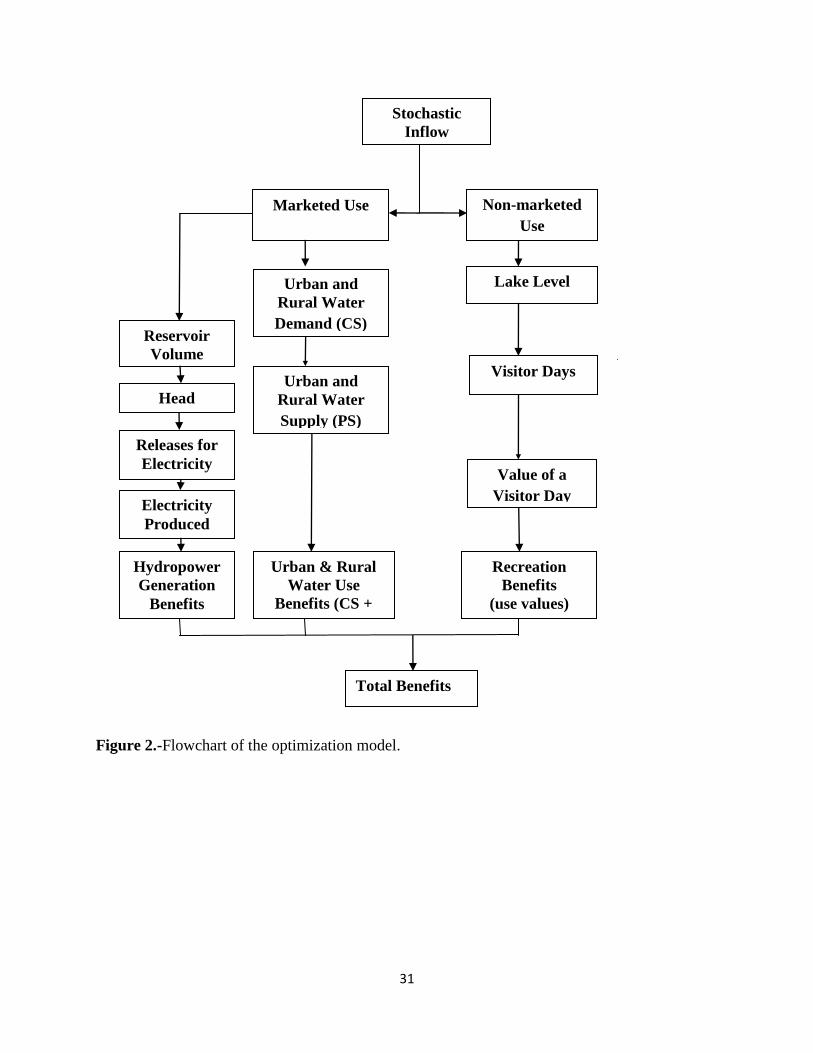
A flowchart representing both hydrologic and economic characteristics of the model is
presented in Figure 2. As shown in this schematic representation, total stochastic inflow of water
was distributed among marketed (urban and rural water supply and hydropower uses) and non-
marketed1 (recreation) uses. The economic benefits derived from recreational uses was obtained
by multiplying visitor days (visitors times the average number of days they spend at the lake) by
the value of a visitor day. Economic benefits of hydropower production were obtained by
multiplying the amount of hydropower produced based on the water released for this purpose and
the head of the reservoir, i.e. average lake level above the turbine by price of electricity.
Economic benefits arising from urban and rural water supply uses depend on consumer surplus
plus producer surplus derived from monthly/weekly water demand (the area below the demand
curve and above the supply curve).
Mathematical Model
A non-linear programming model developed for the Broken Bow reservoir in Oklahoma
(Mckenzie 2003) was modified to allocate Lake Tenkiller water among competing uses given
stochastic monthly or weekly inflows, on-peak and off-peak water demand for hydroelectricity,
urban and rural water supply, and recreational uses for the year 2010. The Frontline Risk Solver
(Fylstra 2010) was used to solve the model. Total net expected economic benefits were
1 In this study non-market valuation is limited to only “use values”. A more extensive study could include “non-use
values such as existence value, bequest values and option values. Thus, restricting the study to use values suggest
more conservative results.

6
maximized over a year period by controlling monthly/weekly releases for hydroelectric power
generation, and urban and rural water supply uses. The limited capacity of the Risk Solver
limited problem size. So stochastic inflows were modeled monthly except during June, July, and
August where they were modeled on a weekly basis. A mass balance equation was used to
determine the monthly/weekly level and volume of water in the lake given the inflows and
outflows. The model was specified as:
Maximize:
))()(()(1
tt
T
t
t URBRBEHBETBE
, (1)
where E(TB) = Expected total economic benefits for the year 2010, E(HBt) = Expected
hydroelectric power generation benefits in month/week t, E(RBt) = Expected recreational
benefits in month/week t, and URBt = Urban and rural water supply benefits in month/week t and
T is the combinations of month and week for the year 2010.
According to USACE (2010C), top of the flood pool for Lake Tenkiller is 667 famsl.
Flood risk management in the model is implicitly considered by always maintaining the lake
level below 6402 famsl. An upper bound of 640 famsl was imposed on the lake level to maintain
flood control capacity. The reservoir mass balance equation (Mckenzie 2003) determines the
ending monthly/weekly reservoir volume from the beginning volume plus expected inflows
(including precipitation), and less outflows (hydropower generation releases and other releases),
and evaporation:
ttttt+ - Ε- Ο Ι + E = VV )(1 (2)
Vmin ≤ Vt ≤ Vmax, Omin ≤ Ot≤ Omax, Vt, It, Ot ≥ 0,
2 8 to 10 feet rise of lake level above the normal pool of 632 famsl results in the picnic area under water. Therefore,
in this study conservatively flood pool level was considered at 640 famsl.

7
where Vt+1 = Volume of water in the reservoir in month/week t+1, Vt = Volume of water in the
reservoir in month/week t, E(It) = Expected inflow of water to the reservoir in month/week t, Ot
= Outflows of water from the reservoir in month/week t, and Et = Evaporation of water from the
reservoir in month/week t, Vmin = Minimum volume of water in the reservoir, Vmax = Maximum
volume of water in the reservoir, Omin = average minimum historical outflows of water from the
reservoir, and Omin = average maximum historical outflows of water from the reservoir. The
bounds on the downstream releases are to protect the trout fishery of lower Illinois river, which
is around ten miles below the dam.
Monthly inflows were tested as to whether or not they could be modeled lognormal
distributions (Wang et al. 2005). The acceptability of using the lognormal function to represent
reservoir inflows over the October 1979 - May 2010 (USACE 2010a, 2010b) period was
confirmed with the Kolmogorov-Smirnov goodness of fit test (Phillips 1972). Simulated average
monthly/weekly inflows and their standard deviations were compared against the historical
monthly/weekly inflows mean and standard deviations, as shown in Table 1.
Hydroelectric Power Generation Benefits
The economic benefits arising from hydroelectric power generation was obtained by
multiplying the amount of electricity produced in each period by the price of electricity (USEIA
2010) for that particular period. Southwestern Power Administration (SWPA) delivered the total
amount of hydroelectricity generated by Lake Tenkiller to the not-for-profit Oklahoma
Municipal Electric Systems at a rate of 2.8 cents per kilowatt-hour (SWPA 2007). However, in
this study, both average wholesale and retail monthly electricity prices were used (USEIA 2010).
Table 2, shows peak and normal average wholesale and retail hydroelectric price used in this
study. Whether incremental amounts of electricity should be valued at the wholesale or retail
8
price depends on the marginal costs of distribution. If the marginal distribution cost is very low
the retail price serves as an upper bound. If the marginal distribution cost is very high, the
wholesale price serves as the lower bound for electricity values. It was assumed that all
electricity generated between 3 pm through 7 pm during the summer months of June, July and
August was sold at a peak rate that was $0.02 per kilowatt hour (OEC 2010) above the wholesale
or retail market price for that particular period.
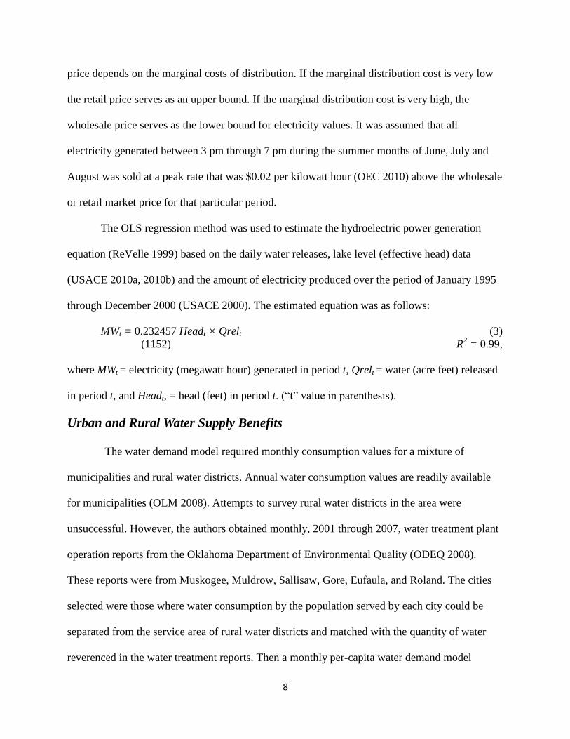
The OLS regression method was used to estimate the hydroelectric power generation
equation (ReVelle 1999) based on the daily water releases, lake level (effective head) data
(USACE 2010a, 2010b) and the amount of electricity produced over the period of January 1995
through December 2000 (USACE 2000). The estimated equation was as follows:
MWt = 0.232457 Headt × Qrelt (3)
(1152) R2 = 0.99,
where MWt = electricity (megawatt hour) generated in period t, Qrelt = water (acre feet) released
in period t, and Headt, = head (feet) in period t. (“t” value in parenthesis).
Urban and Rural Water Supply Benefits
The water demand model required monthly consumption values for a mixture of
municipalities and rural water districts. Annual water consumption values are readily available
for municipalities (OLM 2008). Attempts to survey rural water districts in the area were
unsuccessful. However, the authors obtained monthly, 2001 through 2007, water treatment plant
operation reports from the Oklahoma Department of Environmental Quality (ODEQ 2008).
These reports were from Muskogee, Muldrow, Sallisaw, Gore, Eufaula, and Roland. The cities
selected were those where water consumption by the population served by each city could be
separated from the service area of rural water districts and matched with the quantity of water
reverenced in the water treatment reports. Then a monthly per-capita water demand model
9
(Borland, 1998) was estimated using SAS PROC MIXED (Littell et al. 2008). The city and
annual variables were considered to be random.
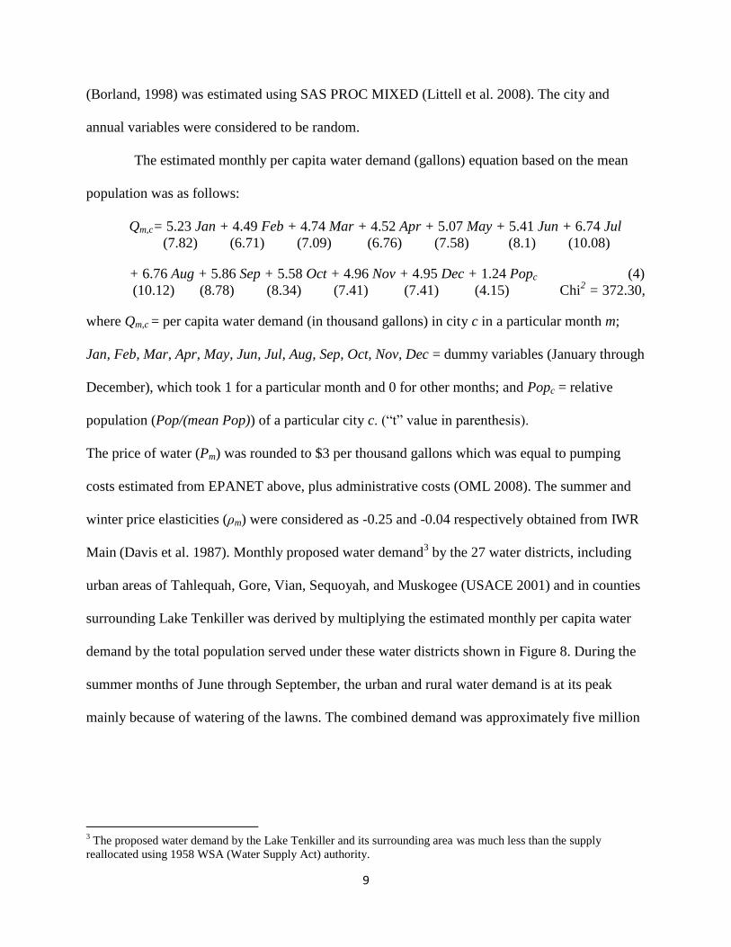
The estimated monthly per capita water demand (gallons) equation based on the mean
population was as follows:
Qm,c= 5.23 Jan + 4.49 Feb + 4.74 Mar + 4.52 Apr + 5.07 May + 5.41 Jun + 6.74 Jul
(7.82) (6.71) (7.09) (6.76) (7.58) (8.1) (10.08)
+ 6.76 Aug + 5.86 Sep + 5.58 Oct + 4.96 Nov + 4.95 Dec + 1.24 Popc (4)
(10.12) (8.78) (8.34) (7.41) (7.41) (4.15) Chi2 = 372.30,
where Qm,c = per capita water demand (in thousand gallons) in city c in a particular month m;
Jan, Feb, Mar, Apr, May, Jun, Jul, Aug, Sep, Oct, Nov, Dec = dummy variables (January through
December), which took 1 for a particular month and 0 for other months; and Popc = relative
population (Pop/(mean Pop)) of a particular city c. (“t” value in parenthesis).
The price of water (Pm) was rounded to $3 per thousand gallons which was equal to pumping
costs estimated from EPANET above, plus administrative costs (OML 2008). The summer and
winter price elasticities (ρm) were considered as -0.25 and -0.04 respectively obtained from IWR
Main (Davis et al. 1987). Monthly proposed water demand3 by the 27 water districts, including
urban areas of Tahlequah, Gore, Vian, Sequoyah, and Muskogee (USACE 2001) and in counties
surrounding Lake Tenkiller was derived by multiplying the estimated monthly per capita water
demand by the total population served under these water districts shown in Figure 8. During the
summer months of June through September, the urban and rural water demand is at its peak
mainly because of watering of the lawns. The combined demand was approximately five million
3 The proposed water demand by the Lake Tenkiller and its surrounding area was much less than the supply
reallocated using 1958 WSA (Water Supply Act) authority.
10
gallons per day. The consumer surplus4 derived from urban and rural water supply was
calculated by integrating the price flexibility form of the demand function.
ttt
Q
tt dQQCSt
)(0
, (5)
where CSt = consumer surplus in month/week t, αt = (Pt – δt Qt) intercept of the inverse demand
function, and δt = (Pt /Qt)×(1/ρt) slope of the inverse demand function.
The total welfare derived from urban and rural water supplies was obtained by
subtracting the supply (pumping) cost from the consumer surplus.
Lake Recreation Benefits
In this study, the assumption that the number of monthly lake visitor was dependent on
deviations of the lake from its normal level of 632 famsl was tested using monthly data from
1955 through 2010. Monthly visitor data from the period of 1975 through 2010 September were
obtained from USACE (2010a). Secondary data over the period of 1955 through 1974 published
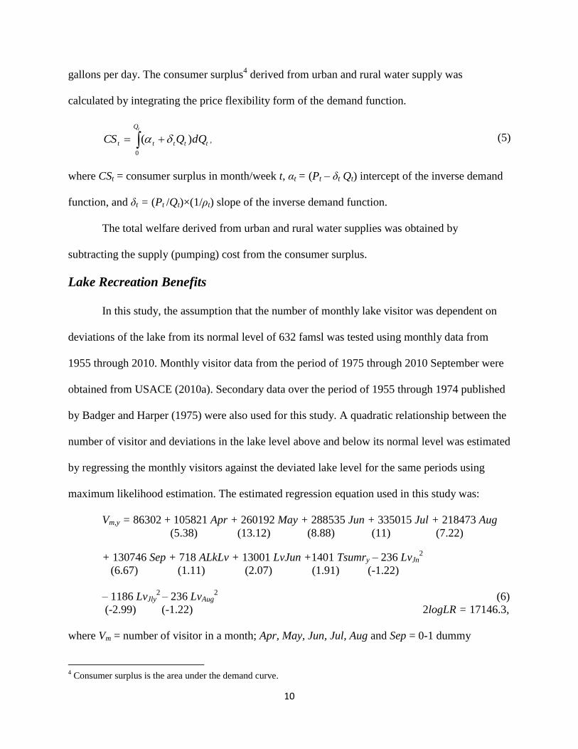
by Badger and Harper (1975) were also used for this study. A quadratic relationship between the
number of visitor and deviations in the lake level above and below its normal level was estimated
by regressing the monthly visitors against the deviated lake level for the same periods using
maximum likelihood estimation. The estimated regression equation used in this study was:
Vm,y = 86302 + 105821 Apr + 260192 May + 288535 Jun + 335015 Jul + 218473 Aug
(5.38) (13.12) (8.88) (11) (7.22)
+ 130746 Sep + 718 ALkLv + 13001 LvJun +1401 Tsumry – 236 LvJn2
(6.67) (1.11) (2.07) (1.91) (-1.22)
– 1186 LvJly2
– 236 LvAug2
(6)
(-2.99) (-1.22) 2logLR = 17146.3,
where Vm = number of visitor in a month; Apr, May, Jun, Jul, Aug and Sep = 0-1 dummy
4 Consumer surplus is the area under the demand curve.

11
variables which were 1 in the indicated month and zero otherwise; Tsumry = time trend for
months June, July, and August (the number of visitor in other months did not vary significantly
with time)for the year y; ALkLv = difference between the actual and normal lake level (632
famsl) when the lake level is below the normal level else zero; LvJun = discrete variable to test if
visits to the lake in June were more sensitive to lake levels than in other months; LvJn2, LvJly
2,
LvAug2 = squares of the difference between the actual and normal lake level (632 famsl) for the
months of June, July, and August respectively (“t” value in parenthesis). The only significant
trend in the number of visitor was during June, July, and August. The time trend in summer
visitors 1401, is measured by the variable Tsumry. The effect of the LvJun variable when
combined with the ALkLv (average lake level) and the quadratic terms is to make the June
visitors more sensitive with respect to lake levels above and below the normal level as shown in
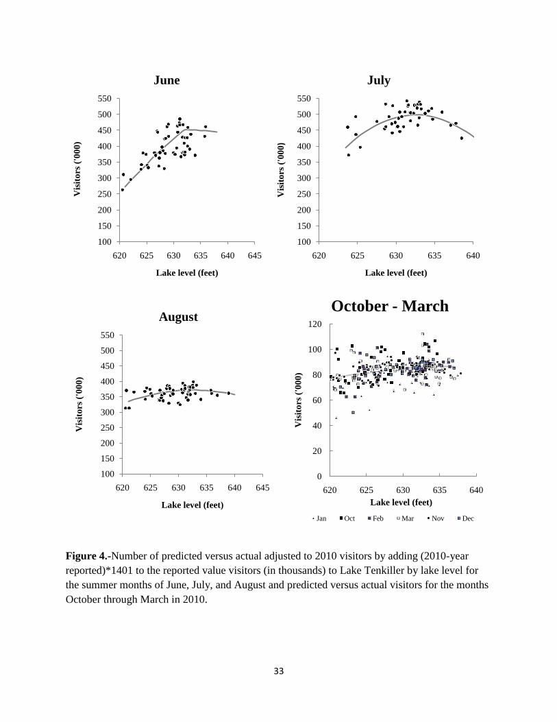
panel a of Figure 4.
The number of monthly visitors was found to increase with lake levels until it reached the
normal level of 632 famsl in June, July, and August, mainly because the visitors are sensitive to
the lake level for Lake Tenkiller, which is famous for skiing, hiking and scuba diving. As
implied by the quadratic lake level terms in equation 6, the number of visitors began to decline
when the lake level increased above 632 famsl during the months of June, July and August. Any
lake level below the normal pool will reduce the depth for scuba divers while any level above the
normal pool will results in the flash flood and also increase the navigational hazard. Figure 4
shows the effect of the lake level on visitors in July was stronger than in June or August. It
should be noted that both the predicted number of visitors at each lake level and the actual
number of visitors have been adjusted to 2010 values. The actual number of visitor has been
adjusted upward by an amount equal (2010 –Year reported)*1401, where 1,401 in the summer

12
time trend coefficient mentioned earlier. Finally, monthly visitors were then converted into
visitor days by multiplying the total monthly visitors by the average number of days each visitor
spend at the lake. However, for Lake Tenkiller on average each visitor spends a single day at the
lake (USACE 2010a).
According to economic guidance memorandum (Carlson, 2009) based on the unit day
value method, the value of a visitor day ranges between $3.54 and $10.63 for general recreation.
However, Gajanan et al. (1998) found that the economic value of lake recreation derived from
motor boating and waterskiing ranges between $9.85 and $45.61, and it varies across different
ecoregions in United States. Boyer et al. (2008) estimated the recreational value of Lake
Tenkiller as part of a larger random utility travel cost model for all lakes in Oklahoma and found
the value of a visitor day to Lake Tenkiller was around $191 in 2008, the highest value for any
Oklahoma lake. Badger and Harper (1975) using travel cost method found that the value of a
visitor day at Lake Tenkiller was $4.67, which is equivalent to around $24 in 2010 prices.
Two values for a visitor day were used in this study. The low value was $10 per visitor
day as per Carlson (2009). The upper value was $50 per day (about one-fourth the value
estimated by Boyer et al. (2008)).
An additional study by Roberts et al. (2008) had shown that the willingness to pay for a
visitor day at Lake Tenkiller declined by $0.82 for each foot the lake was below the normal
level. Figure 5(a) and 5(b) show how the value of a visitor day was decreased in the model from
$50 and $10 (when the lake level was 632 famsl or more), to $43 and $3 per day (when the lake
level was 624 famsl or less). Total recreational benefits were calculated by multiplying the
visitor days (obtained from the estimated number of visitor) by the value of a visitor day at the
indicated lake level. Table 3, shows the recreational benefits derived from different lake levels

13
for the month of August 2010. This study is also unique as both the number of visitor and the
value of a visitor day vary with the level of the reservoir.
Results
Effect of Including Recreation as an Optimizing Variable
Effect of explicitly including or not including recreation benefits in the lake management
optimization function (Objective 2) and its impact on the net economic benefits were measured
by comparing two scenarios. In the first scenario, economic benefits were maximized with
respect to releases for hydropower generation, and public water supply uses only. Recreational
benefits were calculated post optimization from resulting lake levels. In the second scenario, net
economic benefits were maximized with respect to recreation, hydropower generation, and
public water supply. Hydropower was assumed to be sold at the peak retail electricity prices
shown in Table 2 and the base visitor day was assumed to be worth $50 in both scenarios. Table
4 shows that net annual economic benefits were $214.09 million when optimized with respect to
hydropower and public water supply use, and recreation benefits were determined after the
optimization. When recreational benefits were directly considered in the economic optimization
model (scenario 2), the net annual economic benefits were $217.77 million. The estimated
annual gain of $3.68 million from the lake resource was approximately 1.72 percent. Recreation
benefits were increased by $3.8 million or three percent while the value of hydropower
generation declined by approximately $0.09 million, shown in Figure 9. The ratio of the increase
in recreation benefits per dollar of hydropower loss was 42 to 1. Public water supply uses
remained essentially unchanged between scenarios 1 and 2, because in the case of Lake
Tenkiller, the proposed demand for domestic water use is much more inelastic than the demand
for recreational and hydropower generation use.

14
When focusing on hydropower in scenario 1, the optimal strategy was to raise lake levels
from the normal 632 to 640 feet above mean sea level (Figure 6), to increase head and power
generation during the summer months when both hydropower price and demand were at their
peak. However, when recreation was considered (scenario 2), in the objective function, the
optimal strategy was to maintain levels slightly above the normal pool of 632 famsl from May
through mid August and maximize visitor numbers during the summer. It should be noted that
historical levels are very close to scenario 2 levels on May and June but are lower from July
through October. This indicates the current management strategy is not one of strictly
maximizing hydropower production.
The model was further used to calculate the net economic benefits given the historical
average lake levels shown in Figure 6. The purpose was to estimate the net total economic
benefits that would be obtained in the year 2010 if the lake levels were constrained to average
historical lake levels of years 1979-2010, with estimated 2010 visitor numbers and public water
demands. It was found that for year 2010, total annual economic benefits derived from the
average historical lake levels would be around $215.03 million, which was around $2.74 million
lower than in scenario 2, with recreation benefits in the objective function. That is, the historical
(1979-2010) levels were near optimal shown in Figure 6 except for July through October. One of
the reasons for these levels is the early draw down to meet the peak electricity demand. It is also
worth noting that optimal lake levels obtained from the stochastic optimization model are higher
and much closer to the historical levels than the levels obtained under deterministic optimization
shown in Figure 7. This is because with lognormal inflows, the mean inflow is greater than the
more likely median inflow. Releasing more water under the expectation of receiving a mean
inflow would increase the number of years when the actual level was below normal. There was

15
around $219.87 million total economic benefits derived under deterministic condition which was
around $2.10 million higher than the stochastic solution. The comparison of the total economic
benefits among these three different situations (stochastic, deterministic and historical) was
shown in Figure 10. The optimal stochastic lake levels from June through mid-July are almost
identical to the average historical levels.
Sensitivity of Optimal Lake Levels to Recreation Values and Electricity Prices
Further the model was solved with three different combinations of values for a visitor day
and peak electricity prices. These combinations were: (i) $50 value of a visitor day – peak retail
hydroelectricity prices, (ii) $10 value of a visitor day – peak retail hydroelectricity prices and (iii)
$10 value of a visitor day – peak wholesale hydroelectricity prices. These are scenarios 2, 3, and
4 respectively. Optimal number of visitor and the amount of hydropower produced under 2, 3,
and 4 are shown in Table 4. The results show there is very little different between the three
solutions. That is even when recreation is valued at $10 per day and electricity is prices at peak
retail rates, there was a little increase in hydropower production when the electric prices
increased from wholesale to retail and the value of a visitor day was decreased from $50 to $10.
The optimal August lake level remains above the average historical August level for all three
scenarios shown in Figure 8. However, maintaining a normal lake level of around 632 famsl
during the summer months of June, July, and August for Lake Tenkiller was beneficial to
maximize both the recreational and hydropower generation benefits since any lake level above
and below the normal lake level of 632 famsl would definitely reduce the number of visitor for
those months. By contrast, in the model where hydroelectric power generation benefits were the
main concern of the management (lake recreational benefits were not included in the objective
function), then it would be beneficial to increase the lake level (head) above the turbine and

16
release water during the summer months when the electricity price was at its peak. The results
show that during June, July, and August, when the number of visitor was at its peak, the lake
level should be maintained two to three feet above the normal lake level of 632 famsl and some
of the releases for hydroelectric power generation should be shifted to the spring and fall periods.
The Scenario 2 results predict that there were around 241,018 more visitors compared to scenario
1, if the lake level were maintained slightly above the normal level through mid August, as
shown in Figure 11. The main increase of 188,118 visitors was predicted to occur in July.
In Table 6, the August visitor days were predicted to reach a maximum of 381,830 visitor
days at the normal lake level of 632 famsl (Table 3). So, as the level is lowered from 637 to 636
famsl, additional 13.72 thousand acre feet are released and $88.34 thousand dollars of electricity
are generated. As the lake level is lowered toward normal (from 637 to 636 feet), the number of
visitor increases, adding and $21.24 thousand in recreational benefits for a total of $109.58
thousand. The total value of economic benefits derived from the lake resource continues to
increase though by smaller amounts until the lake level has reached 632 famsl. At this level, for
the month of August, there is the highest number of visitor days (Table 3). The increase in the
aggregate lake value is the change in the value of electricity produced plus the gain in the
recreational value (number of visitor days multiplied by $10 per day). However, as the level is
lowered below 632 the value of the visitor day declines as shown in Figure 5b. While the decline
from $10 per day at 632 famsl to $9.18 famsl seems small, the value of total recreation benefits
at 631 feet is obtained by multiplying 380,886 visitor days by $9.18 (Table 3). Thus, the value of
recreation benefits declines by $321,858 for the one foot decline between 632 and 631 famsl
which are three times greater than the value of additional electricity generated. Thus, for Lake
Tenkiller, the finding is that total economic benefits derived from the lake resource are

17
maximized by maintaining the lake level two to three feet above normal in June, July and
declining to the normal lake level of 632 famsl by mid August. That is inclusion of recreation
values as a variable in the optimization model indicates a higher than the historical level should
be maintained during July and August to increase recreational benefits.
Results obtained from this optimization model satisfy the equi-marginal principle while
allocating Lake Tenkiller water among (a) recreational use, (b) hydroelectric power generation
use, and (c) urban and rural water supply use. That is, it is not possible to take one additional
acre foot of water from hydropower and transfer it to urban and rural water use or to recreational
use and increase the total economic benefits arising from Lake Tenkiller water uses. The
marginal value or shadow price of water in each alternative use must be equal when measured at
the lake. Table 7, column (2) shows the marginal cost of treatment and delivering an acre foot of
water. The marginal price of water delivered for urban and rural water supply use is higher by
the amount of treatment and delivery cost of water supplying to the surrounding area of Lake
Tenkiller ($257.64). This result occurs because the users are usually charged only the cost of
treatment and delivery, but not the cost of holding water for alternative uses. Thus the consumer
receives water at a subsidized rate. The price difference between the true delivered marginal cost
of water and cost of treatment and delivery of one acre foot of water is the opportunity cost (cost
that the lake managers are incurring by not using one acre foot of water for other purposes) of
water at the lake shown in column 7 of Table 7.
Discussion
The results are interesting since neither urban and rural water supply use nor recreational
use was considered the primary uses when the dam was constructed (USACE 2009). The results
show the value of electricity that could be generated by releasing more water and lowering the

18
lake level below the normal level of 632 famsl in the summer period is more than offset by
reduced recreation benefits. This result differs from the results obtained by Ward and Lynch
(1996) for reservoirs in New Mexico. This difference is in part because the number of monthly
summer visitors to Lake Tenkiller varies from 400 to over 500 thousand and there is a change in
willingness to pay due to the change in the lake level, in part, because the head above the
turbines is lower for Lake Tenkiller than for the Rio Chama Basin of New Mexico. It was also
found that in the absence of stochastic inflows the model overestimates total economic benefits.
The optimal management plan is also influenced by the head of the reservoir. If the reservoir had
higher elevation (head) over the turbine, then the value of hydroelectric power generation would
increase relative to the lake recreational benefits. The results indicate that the average lake level
maintained over the years 1979-2010 would provide near optimal 2010 benefits except for mid
July through October. Therefore, for Lake Tenkiller it is suggested that the releases for
hydropower generation should be delayed till mid August
The economic optimization model developed and used in this study is able to test several
different management policies. This type of model could be used to identify the economic
impacts of different types of allocation patterns by controlling the releases. The model’s ability
to allocate water among multiple uses over the different time period under stochastic inflows and
to change the optimal usage pattern under different conditions makes it a unique and valuable
tool for the governmental policy analysis. This model is also helpful in any further cost benefit
analysis since it provides the shadow price (opportunity cost) of water at the lake. The modeling
approach used in this study may be useful for the policy makers to compare different
management scenarios and compare the impact of each strategy on the net economic benefits.

19
This can help water managers and policy makers to test different water management policies and
implement them while managing a reservoir.
Acknowledgements
The authors were grateful to Oklahoma Water Resources Research Institute (OWRRI),
Oklahoma Water Resources Board (OWRB) and U.S. Geological Survey (USGS) for financially
supporting this research work.
References
Badger DD, Harper WM. 1975. Assessment of pool elevation effects on recreation and
concession operations at Tenkiller Ferry Lake. Department of Agricultural Economics,
Oklahoma State University, OK.
Boland JJ. 1998. Forecasting Urban Water Use: Theory and Principles. P. 77-94. In: Baumann
DD, Boland JJ, Hanemann WM, editors. Urban water demand management and planning.
New York (NY): McGraw-Hill, Inc.
Boyer T, Stoecker A, Sanders L. 2008. Decision support model for optimal water pricing
protocol for Oklahoma water planning: Lake Tenkiller case study FY Oklahoma Water
Resource Research Institute, Stillwater OK.
Carson B. 2009. Economics Guidance Memorandum, 10-13, unit day value for recreation, fiscal
year 2010. Department of the Army (USACE), Washington (DC).
Chatterjee B, Howitt RE, Sexton RJ. 1998. The optimal joint provision of water for irrigation
and hydropower. J Environ Econ Manage. 36:295-313.
Changchit C, Terrell MP, 1993. A multiobjective reservoir operation model with stochastic
inflows. Comput Ind. Eng. 24(2): 303-313.
20
Davis WY, DM Rodrigo, Optiz EM, Dziegielewski B, Baumann DD, Boland JJ, 1987. IWR-
MAIN Water Use Forcasting System, Version 5.1: User’s Manual and System
Description, Prepered for U.S. Army Corps of Engineers, Planning and Management
Consultants, Ltd., Carbondale III.
Debnath D, Stoecker A, Boyer T, Sanders L. 2009. Optimal allocation of reservoir water: a case
study of Lake Tenkiller. Southern Agricultural Economic Association, Atlanta.
[EPA] Environmental Protection Agency. "EPANET2".
http://www.epa.gov/nrmrl/wswrd/dw/epanet.html. Accessed 12 June 2008.
Fylstra D. 2010. Frontline Solvers – Developers of the Excel Solver. Nevada (NV): Frontline
Systems Inc.
Gajanan BG, Berstrom J, Teasley RJ, Bowker JM, Cordell HK. 1998. An ecological approach to
the economic valuation of land- and water-based recreation in the United States. Evriron
Manag. 22:69-77.
Hanson TR, Hatch LU, Clonts HC. 2002. Reservoir water level impacts on recreation, property,
and nonuser values. J Am Water Res Assoc. 38:1007-1018.
Littell RC, Milliken GA, Stroup WW, Wolfinger RD, Schabenberger O. 2008. SAS® for mixed
models 2nd
ed. North Calolina (NC): SAS Institute Inc.
Kent MM, Mather M. 2002. What drive U.S. population growth? Pop Bul. 57: 4.
Mckenzie RW. 2003. Examining reservoir managing practices: the optimal provision of water
resources under alternative management scenario. PhD dissertation. Stillwater (OK):
Oklahoma State University.

21
Murry MN, Barbour K, Hill B, Stewart S, Takatsuka Y. 2003. Economic effects of TVA lake
management policy in east Tennessee. Center for Business and Economic Research, The
University of Tennessee, Knoxville, TN.
[OEC] Oklahoma Electric Cooperative. 2010. Electric service rates.
http://www.okcoop.org/services/rates.aspx. Accessed 28 December 2010.
[OML] Oklahoma Municipal League. 2008. Oklahoma municipal utility cost in 2008. A report of
Oklahoma Conference of Mayors (OCOM), Municipal Electric systems of Oklahoma
(MESO).
[OWRB] Oklahoma Water Resources Board 2008. Strategic plan 2008-2012.
[ODEQ] Oklahoma Department of Environmental Quality. 2008. Public Water Supply Systems.
Records from monthly operation reports filed by water system managers. Tulsa (OK).
Phillips DT. 1972. Applied goodness of fit testing. AIIE Monograph, American Institute of Industrial
Engineers, Norcross (GA).
ReVelle C. 1999. Optimizing reservoir resources: including a new model for reservoir reliability,
New York (NY): John Wiley & Sons, Inc.
Roberts D, Boyer T, Lusk J. 2008. Environmental preference under uncertainty. Ecol Econ.
66:584-93.
Serrie J. 2009. Water wars “Man versus Mussel” Fox news blogs.
http://onthescene.blogs.foxnews.com/2009/02/25/water-wars-man-versus-mussel/
Accessed 20 Apr 2010.
Singer JD. 1998. Using SAS PROC MIXED to fit multilevel models, hierarchical models, and
individual growth models. J Edu Behav Stat. 24:323-355
[SWPA] Southwestern Power Administration. 2007. Annual Report. Independent Accounts’
Review Report.

22
[USACE] United States Army Corps of Engineers. 2000. 1995-2000 WCDS Tulsa
District:Tenkiller lake hydropower generation information. http://www.swt-
wc.usace.army.mil/PowerGen.html. Accessed 09 Apr 2008.
[USACE] United States Army Corps of Engineers. 2001. Tenkiller wholesale water treatment
and conveyance system study phase iii- additional preliminary designs and cost estimates,
Tulsa (OK).
[USACE] United States Army Corps of Engineers. 2009. Lake Tenkiller information. USACE.
http://www.tenkiller.net/lakeinfo.html. Accessed 24 Nov 2009.
[USACE] United States Army Corps of Engineers. 2010a. Record of monthly lake attendance:
Lake Tenkiller. Tulsa Districts Office, Tulsa (OK).
[USACE] United States Army Corps of Engineers. 2010b. 1979-1994 Record of monthly charts
for Lake Tenkiller. Tulsa Districts Office, Tulsa (OK).
[USACE] United States Army Corps of Engineers. 2010c. 1995-2010 Monthly charts for
Tenkiller Lake. http://www.swt-wc.usace.army.mil/TENKcharts.html. Accessed 14 Nov
2010.
[USEIA] United States Energy Information Administration. 2010. Current and historical monthly
retail sales, revenues and average revenue per kilowatt-hour by state and by sector (Form
EIA-826). http://www.eia.doe.gov/cneaf/electricity/epm/table5_3.html. Accessed 16 Feb
2010
Wang YC, Yoshitani J, Fukami K. 2005. Stochastic multiobjective optimization of reservoirs in
parallel. Hydrol Process. 19:3551-67.
Ward FA, Lynch TP. 1996. Integrated river basin optimization: modeling economic and
hydrologic interdependence. Water Res Bull. 32:1127-38.

23
Table 1.-Simulated average monthly inflows and standard deviation compared with historical
average inflows and standard deviation (1979-2010).
Historical Inflow (Ac-ft)
Simulated Inflow (Ac-ft)
Month Average
Standard
Deviation Average
Standard
Deviation
Jan 109,190 103,977
109,034 101,854
Feb 109,935 79,689
109,839 78,741
Mar 164,909 116,659
164,752 115,131
Apr 165,468 122,134
165,377 121,443
May 150,209 124,650
150,330 125,042
Jun week 1 26,041 20,695
26,021 20,510
Jun week 2 26,495 28,011
26,442 27,310
Jun week 3 33,492 55,420
33,534 54,739
Jun week 4 23,753 43,666
23,627 40,694
Jul week 1 18,046 26,716
17,966 25,274
Jul week 2 12,774 16,508
12,756 16,033
Jul week 3 8,484 6,621
8,494 6,748
Jul week 4 9,127 10,060
9,117 9,854
Aug week 1 7,366 10,104
7,521 12,792
Aug week 2 8,855 9,634
8,835 9,374
Aug week 3 6,753 5,829
6,760 5,876
Aug week 4 4,927 3,052
4,924 3,031
Sepr 42,178 50,478
42,098 49,152
Oct 67,228 110,225
67,620 114,918
Nov 92,538 95,267
92,449 94,092
Decr 116,470 117,299 116,310 115,115

24
Table 2.-Wholesale and wholesale peak and retail and retail peak
electricity price per kilowatt-hour for the year 2010.
Month
Wholesale
electricity
price
Wholesale
peak
electricity
price
Retail
electricity
price
Retail peak
electricity
price
Jan $0.05 $0.05 $0.07 $0.07
Feb $0.05 $0.05 $0.08 $0.08
Mar $0.04 $0.04 $0.07 $0.07
Apr $0.04 $0.04 $0.07 $0.07
May $0.04 $0.04 $0.07 $0.07
Jun $0.05 $0.07 $0.07 $0.07
Jul $0.05 $0.07 $0.08 $0.10
Aug $0.06 $0.08 $0.08 $0.10
Sep $0.04 $0.04 $0.08 $0.10
Oct $0.03 $0.03 $0.07 $0.07
Nov $0.03 $0.03 $0.07 $0.07
Dec $0.04 $0.04 $0.07 $0.07

25
Table 3.-Visitor days, value of a visitor day starting at $10 and recreational
benefits for different lake levels for the month of August 2010.
Lake level Visitor days
Value of a visitor
day
Recreation
benefits
638 373,334 10.00 3,733,340
637 375,930 10.00 3,759,300
636 378,054 10.00 3,780,540
635 379,706 10.00 3,797,060
634 380,886 10.00 3,808,860
633 381,594 10.00 3,815,940
632 381,830 10.00 3,818,300
631 380,876 9.18 3,496,442
630 379,450 8.36 3,172,202
629 377,552 7.54 2,846,742
628 375,182 6.72 2,521,223

26
Table 4.-Comparison of total economic benefits from Lake Tenkiller when recreational values
were and were not included in the objective function for 2010.
Recreational values in objective
function***
Recreational values not in objective.
function***
Recreation* benefits $ 126,392 Recreation
* Benefits $ 122,593
Hydropower**
benefits $ 6,890 Hydropower**
benefits $ 6,977
Rural water supply (RWS) $ 84,518 Rural water supply (RWS) $ 84,518
Total benefits (with recreation in
objective function) $ 218,099
Total benefits (without recreation
in objective function) $ 206,969
*Recreation valued at $50 per visitor day when lake level is 632 feet and above; **Hydropower valued at the
average monthly retail peak electricity price; ***values in thousand dollars

27
Table 5.-Sensitivity of the estimated number of monthly visitors and hydropower production to
changes in the value of a visitor day from $50 per visitor day to $10 per visitor day when
hydropower is valued at 2010 wholesale or retail peak electricity prices.
Visitors Hydropower-generation
Scenario 2 3 4 2 3 4
Value of a
visitor day $50 $10 $10
$50 $10 $10
Monthly
Electricity
Price Retail Retail Wholesale
Retail Retail Wholesale
Month Number
MwH
Jan 86,302 86,302 86,302
9,235 9,198 9,234
Feb 86,302 86,302 86,302
8,455 8,417 8,454
Mar 86,302 86,302 86,302
11,130 11,140 11,129
Apr 191,597 191,597 191,597
8,917 8,937 8,917
May 345,555 345,555 345,555
13,716 13,717 13,712
Jun week 1 104,851 104,839 104,840
3,144 3,165 3,143
Jun week 2 104,779 104,768 104,772
1,813 1,784 1,812
Jun week 3 105,595 105,583 105,591
2,797 2,818 2,794
Jun week 4 105,568 105,561 105,567
3,391 3,356 3,387
Jul week 1 123,920 123,932 123,916
1,459 1,551 1,458
Jul week 2 124,237 124,237 124,237
2,098 2,119 2,096
Jul week 3 124,180 124,175 124,181
614 618 613
Jul week 4 123,982 123,972 123,981
419 325 419
Aug week 1 92,913 92,910 92,913
385 386 385
Aug week 2 92,827 92,822 92,827
582 584 581
Aug week 3 93,009 93,008 93,009
127 116 127
Aug week 4 92,420 92,430 92,420
731 581 731
Sep 215,739 215,755 215,766
2,520 2,524 2,518
Oct 86,219 86,256 86,244
2,485 2,557 2,483
Nov 86,302 86,302 86,302
9,301 9,656 9,293
Dec 86,302 86,302 86,302
9,494 9,520 9,485
Total 2,558,899 2,558,909 2,558,926
92,812 93,068 92,769

28
Table 6.-Effect of releasing water to create a one foot decline in the lake level from 637 to 630
feet above sea level on hydropower values and recreational benefits for August of 2010.
Level
Volume
of
release
(Ac-Ft)
Changes in
hydro-electric
value*
Change in
number of
visits
Changes in
Recreation
benefits**
Total change
in net
economic
benefits
637-636 13,722 $88,335.03 2,124 21,240 $109,575
636-635 13,524 $86,417.26 1,652 16,520 $102,937
635-634 13,335 $84,571.25 1,180 11,800 $96,371
634-633 13,153 $82,792.14 708 7,080 $89,872
633-632 12,979 $81,075.45 236 2,360 $83,435
632-631 12,811 $79,417.07 -954 -321,858 -$242,441
631-630 12,650 $77,813.36 -1,426 -324,240 -$246,426 *electricity is valued at $0.07 per kilowatt hour; ** value of a visitor day at $10

29
Table 7.-Actual delivery cost of water, acre feet of water released for hydropower production,
megawatt-hours (MwH) of hydropower produced, hydroelectric power generation benefits,
shadow price for hydropower production, and the per unit price of water at the Lake Tenkiller for
the year 2010 obtained from the optimization model when recreation values were included in the
objective function.
Month
Actual
cost of 1
acre foot
of water
Water
releases for
hydro-
power
(acre feet)
Hydro-
power
production
with
recreation
(MwH)
Hydro-power
production
benefits
Shadow
price for per
1000 KwH
of hydro-
power
productiona
Price of
1 acre
foot of
water at
the
lakeb
Jan $263.27 114,721 9,234 $646,358 $70.00 $5.63
Feb $263.82 104,928 8,454 $648,387 $76.70 $6.18
Mar $263.15 136,255 11,129 $751,214 $67.50 $5.51
Apr $263.48 106,039 8,917 $618,847 $69.40 $5.84
May $263.44 165,000 13,712 $957,066 $69.80 $5.80
Jun week 1 $263.68 38,119 3,143 $230,298 $73.27 $6.04
Jun week 2 $263.69 21,946 1,812 $132,774 $73.27 $6.05
Jun week 3 $263.68 33,894 2,794 $204,716 $73.27 $6.04
Jun week 4 $263.61 41,566 3,387 $248,181 $73.27 $5.97
Jul week 1 $263.96 17,911 1,458 $113,218 $77.65 $6.32
Jul week 2 $263.90 25,990 2,096 $162,760 $77.65 $6.26
Jul week 3 $263.90 7,614 613 $47,631 $77.70 $6.26
Jul week 4 $263.90 5,193 419 $32,514 $77.60 $6.26
Aug week 1 $263.91 4,770 385 $29,911 $77.69 $6.27
Aug week 2 $263.91 7,213 581 $45,208 $77.81 $6.27
Aug week 3 $263.92 1,572 127 $9,868 $77.70 $6.28
Aug week 4 $263.89 9,085 731 $56,811 $77.72 $6.25
Sep $263.82 31,224 2,518 $192,846 $76.59 $6.18
Oct $263.75 30,241 2,483 $184,740 $74.40 $6.11
Nov $263.61 114,890 9,293 $685,801 $73.80 $5.97
Dec $263.40 117,551 9,485 $677,240 $71.40 $5.76 Note: Shadow Price: the extra amount of cost incurred in order to produce one additional unit of hydropower
a Column (6) is equal to Column (5) divided by Column (4),
b Column (2) minus $257.64 (supply cost of per acre
foot of water) is equal to column (7), b Column (7) is also equal to Column (5) divided by Column (3)

30
Figure 1.-Lake Tenkiller and its surrounding areas in Northeast Oklahoma.
31
Figure 2.-Flowchart of the optimization model.
Stochastic
Inflow
Reservoir
Volume
Lake Level
Releases for
Electricity
Visitor Days
Electricity
Produced
Recreation
Benefits
(use values)
Hydropower
Generation
Benefits
Urban & Rural
Water Use
Benefits (CS +
PS)
Total Benefits
Marketed Use Non-marketed
Use
Urban and
Rural Water
Demand (CS)
Head
Value of a
Visitor Day
Urban and
Rural Water
Supply (PS)

32
Figure 3.-Predicted urban and rural water demand (acre feet) for each month by the Lake
Tenkiller and its surrounding area for the year 2010.
0
200
400
600
800
1,000
1,200
Jan Feb Mar Apr May Jun Jul Aug Sep Oct Nov DecMo
nth
ly R
ura
l a
nd
Urb
an
Wa
ter D
ema
nd
(Acr
e fe
et)
Month
33
Figure 4.-Number of predicted versus actual adjusted to 2010 visitors by adding (2010-year
reported)*1401 to the reported value visitors (in thousands) to Lake Tenkiller by lake level for
the summer months of June, July, and August and predicted versus actual visitors for the months
October through March in 2010.
100
150
200
250
300
350
400
450
500
550
620 625 630 635 640 645
Vis
ito
rs (
'00
0)
Lake level (feet)
June
100
150
200
250
300
350
400
450
500
550
620 625 630 635 640
Vis
ito
rs (
'00
0)
Lake level (feet)
July
100
150
200
250
300
350
400
450
500
550
620 625 630 635 640 645
Vis
ito
rs (
'00
0)
Lake level (feet)
August
0
20
40
60
80
100
120
620 625 630 635 640
Vis
ito
rs (
'00
0)
Lake level (feet)
October - March
Jan Oct Feb Mar Nov Dec

34
Figure 5a.-$50 per visitor day at Lake Figure 5b.-$10 per visitor day at Lake
Tenkiller as a function of lake level Tenkiller as a function of lake level.
$0
$10
$20
$30
$40
$50
$60
610 620 630 640 650
Va
lue
of
vis
ito
rs d
ay
(V
D)
Lake level (feet)
Value of a visitor day at $50
$0
$10
$20
$30
$40
$50
$60
610 620 630 640 650
Va
lue o
f v
isit
ors
da
y (
VD
)
Lake level (feet)
Value of a visitor day at $10

35
Figure 6.-Comparison between average historical monthly/weekly lake levels for Lake Tenkiller
from 1979-2010 with the optimal lake levels for 2010 when recreational values were and were
not included in the optimization model.
622
624
626
628
630
632
634
636
638
640
642La
ke le
vel
Month/week
Act. Avg With rec. Without rec.

36
Figure 7.-Comparison between average historical monthly/weekly lake levels for Lake Tenkiller
from 1979-2010 with the optimal stochastic lake levels for 2010 and with the optimal
deterministic lake levels for 2010 (recreational values in the objective function).
624
626
628
630
632
634
636
638
640La
ke le
vel
Month/week
Act. Avg Stochastic Deterministic

37
Figure 8.-Optimal lake level with recreational values included in the model for the year 2010
when (i) value of a visitor day is $50 and retail peak price of hydropower; (ii) value of a visitor
day is $10 and retail peak price of hydropower; and (iii) value of a visitor day is $10 and
wholesale peak price of electricity.
620
625
630
635
640
645
650La
ke L
eve
l
Month/week
Optimal lake level with retail peak electricity price and $50 per visitor day
Optimal lake level with retail peak electricity price and $10 per visitor day
Optimal lake level with wholesale peak electricity price and $10 per visitor day

38
Figure 9.-Tradeoff between the loss in hydroelectric power generation values versus gain in lake
recreational values when recreational values were included in the objective function for year
2010.
0.00
0.50
1.00
1.50
2.00
2.50
3.00
3.50
4.00
Gain in rec. Loss in hydro. Unchanged RWS

39
Figure 10.-Comparison between the total economic benefits derived for the year 2010 under
three different situations: Stochastic, deterministic and average historical lake levels.
$212
$213
$214
$215
$216
$217
$218
$219
$220
Stoc Det Hist
Tota
l Be
ne
fits
(m
illio
n)

40
Figure 11.-Comparison of optimal number of monthly visitor for Lake Tenkiller when
recreational benefits were and were not included in the objective function for the year 2010 with
the average historical monthly visitors.
0
50,000
100,000
150,000
200,000
250,000
300,000
350,000
400,000
450,000
500,000
Jan Feb Mar Apr May Jun Jul Aug Sep Oct Nov Dec
Vis
ito
rs
Month
Average actual visitors
Optimal projected 2010 visitors with recreation values
Optimal projected 2010 visitors without recreation values