integrated source/receptor- influence analysisintegrated source/receptor- based methods for source...

Integrated Source/Receptor- Based Methods for Source Apportionment and Area of

Influence Analysis

U.S. EPA STAR PM Source ApportionmentProgress Review Workshop

June 21, 2007

Jaemeen Park, Talat Odman, Yongtao Hu, Florian Habermacher, and Ted RussellGeorgia Institute of Technology

Overview

• Introduction• Source apportionment of PM2.5

– Primary PM2.5 using CMAQ– Regional/Secondary PM2.5 using CMAQ-DDM– Improving emission inventories

• Using metal tracer species• Inverse modeling using CMAQ-DDM

• Area of Influence Analysis

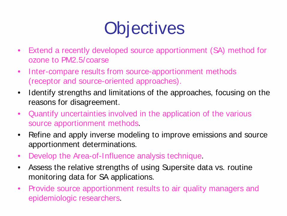
Objectives• Extend a recently developed source apportionment (SA) method for

ozone to PM2.5/coarse• Inter-compare results from source-apportionment methods

(receptor and source-oriented approaches).• Identify strengths and limitations of the approaches, focusing on the

reasons for disagreement.• Quantify uncertainties involved in the application of the various

source apportionment methods.• Refine and apply inverse modeling to improve emissions and source

apportionment determinations.• Develop the Area-of-Influence analysis technique.• Assess the relative strengths of using Supersite data vs. routine

monitoring data for SA applications.• Provide source apportionment results to air quality managers and

epidemiologic researchers.

Approach• Apply various modeling tools to conduct source apportionments

– CMAQ-DDM3D– CMB

• Regular, Molecular Marker, LGO w/gases

– PMF– Inverse modeling (CMAQ-DDM-FDDA)

• Use the extensive data from the Supersites, SEARCH, ASACA and STN– Focus on SE, particularly Atlanta:

• Atlanta Supersite: Extensive PM and gaseous data in summer 1999• SEARCH: SE, detailed PM and gaseous data since 1998• ASACA: Atlanta, daily PM composition since 1999

– Larger scale focus using ESP data (July-August, 2001; January, 2002)

• Conduct uncertainty assessments

Study Area and Periods

SEARCH monitoring sites• Urban sites : Atlanta, Jefferson St. (JST) Birmingham

(BHM), Gulf port (GFP), Pensacola (PNS)• Suburban sites: Pensacola (OLF)• Rural sites: Oak Grove (OAK), Centreville (CTR),

Yorkshire (YRK)

Modeling periods:August 1999July 2001 January 2002July 2005January 2006

Base inventoriesEPA NEI

Point sources in GeorgiaEPA NEI 2002 (draft),

CEM dataForest fire, land clearing debris in 2002

VISTAS, 2005Residential meat cooking

New emissions were added

ASACA

Presenter�

Presentation Notes�

JST and CTR sites were used for comparisons among CMAQ, CMB-RG and PMF results in order to see that accuracy of CMAQ results may affect �

DDM-Sensitivity analysis based Source Apportionment

• Given a system, find how the state (concentrations) responds to incremental changes in the input and model parameters:

Inputs (P)

ModelParameters

(P)

Model

Sensitivity Parameters:

State Variables:( )( )C x,t

( )S C Pij

i

jx, t =

⎛

⎝⎜

⎞

⎠⎟

∂∂

If Pj are emissions, Sij are the sensitivities/responses to emission changes, e.g.., the sensitivity of ozone to Atlanta NOx emissions

• Define first order sensitivities as

• Take derivatives of

• Solve sensitivity equations simultaneously

jiij ECS ∂∂= /)1(

Sensitivity Analysis with Decoupled Direct Method (DDM):

The Power of the Derivative

iiiii ERCC

tC

++∇∇+−∇=∂∂ )()( Ku

iiiii ERCC

tC K u ++∇∇+∇−=∂∂ )()(

Advection Diffusion Chemistry Emissions

ijijijij ESSt

Sij )( )( δ++∇∇+∇−=

∂

∂JSKu

DDM compared to Brute Force

Emissions of SO2

Sul

fate

j

iij

CSε∂∂

=

EB EA

CB

CA

bA

BAij

CCSεε −

−≈

CΔ

EΔ

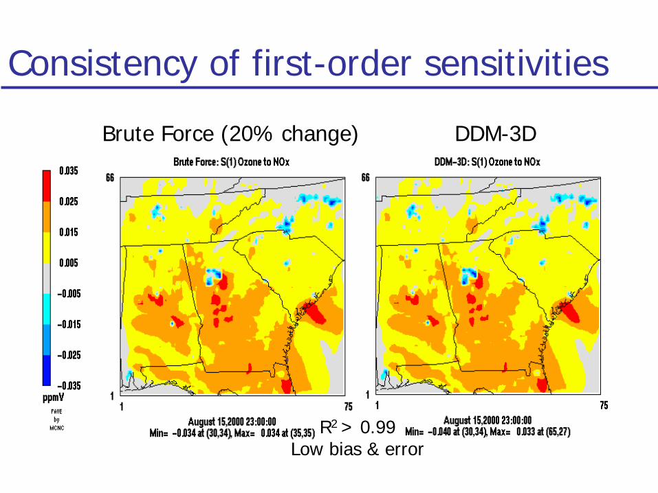
Consistency of first-order sensitivities

Brute Force (20% change) DDM-3D

R2 > 0.99Low bias & error

Advantages of DDM-3D•

Computes sensitivities of all modeled species to many different parameters in one simulation–

Can “tell”

model to give sensitivities to 10s of parameters in the same run

•

Captures small perturbations in input parameters–

Strangely wonderful•

Avoids numerical errors sometimes present in sensitivities calculated with Brute Force

•

Lowers the requirement for computational resources

Evidence of Numerical Errors in BF

NH4

sensitivity to domain-wide SO2

reductions

NOx reductions at a point

In recent study, brute force led to multiple maxima and minima being due to noise.

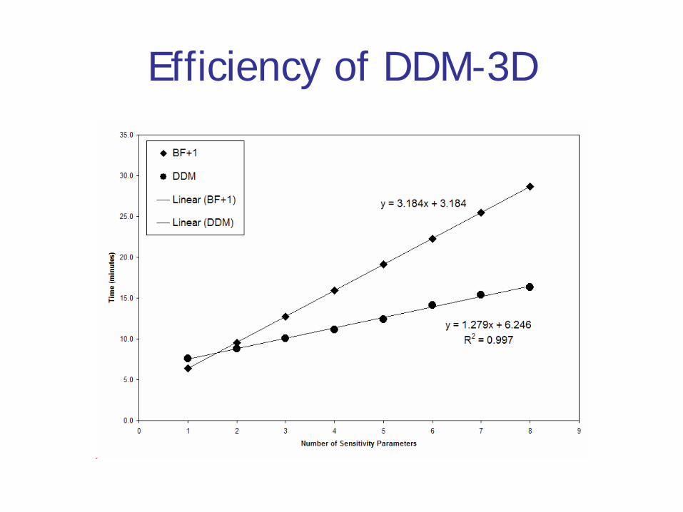
Efficiency of DDM-3D

Regional Source Apportionment of PM 2.5

Using Direct Sensitivity: Application to GeorgiaSources of Atlanta PM2.5

-5

0

5

10

15

20

11.98 17.98 20.92 12.82 10.46 19.54 19.59 15.54 18.87 24.83 25.60 24.37 18.54

6-Jul 7-Jul 8-Jul 9-Jul 10-Jul 11-Jul 12-Jul 13-Jul 14-Jul 15-Jul 16-Jul 17-Julaverage

Date and Concentration (ug/m3)

Sens

itivi

ty (u

g/m

3)

BC SO2BC ANH4BC ASO4Primary* ECPrimary* OCPrimary* SO4Other SecondarySC VOCSC SO2SC NOxNC VOCNC SO2NC NOxTN VOCTN NH3TN SO2TN NOxAL NH3AL SO2AL NOxN.GA NH3N.GA NOxBranch SO2Branch NOxAtlanta VOCAtlanta NH3Atlanta SO2Atlanta NOx

Intercomparison of Source Apportionment Methods

• Apply a variety of methods to relatively rich data base of PM in the SE– Supersite, SEARCH, ASACA, STN

• Methods– CMAQ-DDM– PMF– CMB-Regular (typical anaysis using STN-type data)– CMB-Molecular Marker (using organic molecular speciation)– CMB-LGO (optimized, using gas phase species, w/wo re-

optimization of source profiles)• Adding gaseous species really helps: Don’t stop monitoring CO, SO2

and NOx!• Re-optimization of profiles made smaller difference

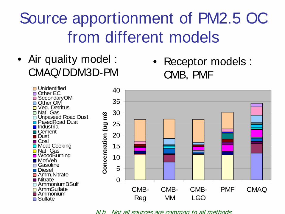
Source apportionment of PM2.5 OC from different models

• Air quality model : CMAQ/DDM3D-PM

0

5

10

1520

25

30

35

40

CMB-Reg

CMB-MM

CMB-LGO

PMF CMAQ

Con

cent

ratio

n (u

g m

3

UnidentifiedOther ECSecondaryOMOther OMVeg. DetritusNat. GasUnpaveed Road DustPavedRoad DustIndustrialCementDustCoalMeat CookingNat. GasWoodBurningMotVehGasolineDieselAmm.NitrateNitrateAmmoniumBSulfAmmSulfateAmmoniumSulfate

• Receptor models : CMB, PMF

N.b. Not all sources are common to all methods

Looking at Uncertainties: Monte Carlo Analysis of CMB with Latin Hypercube Sampling (LHS)

•

Assume log-normally distributed variables in source profiles and ambient data•

PM2.5 data from Atlanta, GA (EPA STN): Jan 02 ~ Nov 03 (# of data points: 212)

•

Construct CDF for each variable using uncertainties•

Divide into 500 equal probable intervals

•

Sample from each variable PDF 500 times•

Constrain source profiles

•

500 simulations using CMB

1.0

0.8

0.6

0.4

0.2

0.0

Cum

ulat

ive

Prob

abilit

y

2.82.62.42.2random variable, x

)1(1∑=

≤n

iif

Uncertainty vs. Source Contribution

6

5

4

3

2

1

0

Unc

erta

inty

, μg/

m3

1612840

Source Cont, μg/m3

CMB defaultMC-LHS

NH4HSO4

1:1

1:2

5

4

3

2

1

0U

ncer

tain

ty, μ

g/m

3121086420

Source Cont, μg/m3

CMB dafaultMC-LHS

(NH4)2SO4

1:1

1:2

1

0

Unc

erta

inty

, μg/

m3

86420

Source Cont, μg/m3

NH4NO3

1:1

1:2

CMB defaultMC-LHS

2

1

0

Unc

erta

inty

, μg/

m3

1086420Source Cont, μg/m3

CMB dafaultMC-LHS

Wood Burning

1:1 1:2

2

1

0

Unc

erta

inty

, μg/

m3


CMB dafaultMC-LHS

Motor Vehicles

1:1 1:2

2

1

0

Unc

erta

inty

, μg/

m3

543210

Source Cont, μg/m3

CMB dafaultMC-LHS

Dust

1:1 1:2

If Sj < jsσ non-detectable source

Uncertainty vs. Source Contribution

2

1

0

Unc

erta

inty

, μg/

m3


CMB dafaultMC-LHS

Pulp &Paper Pro.

1:1

1:2

4

3

2

1

0

Unc

erta

inty

, μg/

m3


CMB dafaultMC-LHS

Coal Power Plant

1:1

1:2

2.0

1.5

1.0

0.5

0.0

Unc

erta

inty

, μg/

m3


CMB dafaultMC-LHS

Mineral Pro.

1:1

1:2

5

4

3

2

1

0

Unc

erta

inty

, μg/

m3


CMB dafault500 runs

Oil Combustion

1:1

1:2

1.2

1.0

0.8

0.6

0.4

0.2

0.0

Unc

erta

inty

, μg/

m3

0.80.60.40.20.0Source Cont, μg/m3

CMB dafaultMC-LHS

Metal Pro.

1:1

1:2

If Sj < jsσ non-detectable source

Daily Variation: PMF vs. CMB-LGO

1 7 12 14 15 16 17 18 19 20 21 22 23 24 25 26 27 28 29 30 31

Monthly Average0

5

10

15

20

25

30

Wood SmokeNitrateCoal combustion SulfateIndustry factor 2Soil Industry factor 1Motor VehicleUndeterminedFine mass

JST, Jan., 2002

Sampling date

CMB Source Apportionment

0

5

10

15

20

25

30

1/14/

02

1/16/

02

1/18/0

2

1/20/0

2

1/22/0

2

1/24/

02

1/26/

02

1/28/

02

1/30/

02

OTHROCM.V.SDUSTCEMSulfateCFPPAMNITRBURN

PMF

Note daily variability in relative source contributions

0

1

2

3

0 1 2 3

CMAQ (36km) [μg m-3]

CM

B-M

M [ μ

g m

-3]

Averaged contribution over the eight SEARCH stations for July 2001 and January 2002

Diesel GasolinePower Plant Road DustWood Burning Meat CookingNatural Gas Other organic massOther mass

r = 0.74 CMB = 1.04 * CMAQ

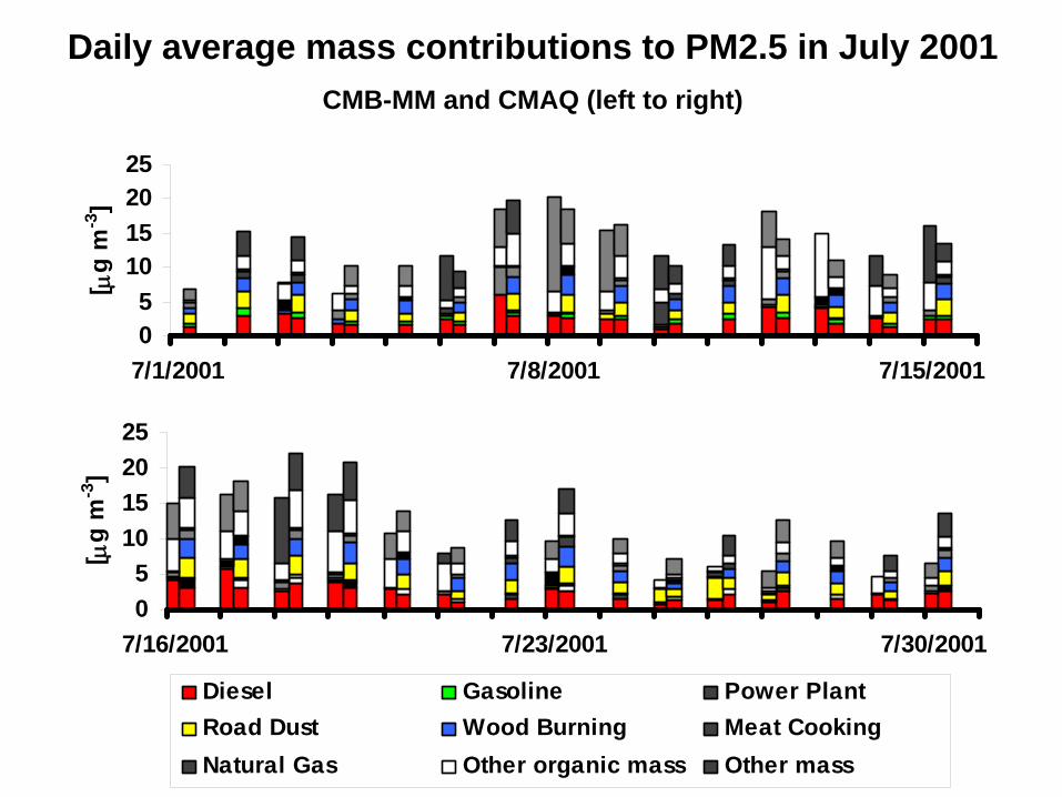
Mass contributions to PM2.5: Comparison of CMB-MM and CMAQ

•

Average of source contributions looks pretty good, particularly just looking at source impacts, but…

Disaggregated some: not so good•

If we look at the results by specific source at individual stations, not quite so good, and further, look at daily agreement…

0

2

4

0 2 4

CMAQ (36km)[μg m-3]

CM

B-M

M [ μ

g m

-3]

Monthly contributions in SEARCH stations

for July 2001 and January 2002

DieselGasolineRoad dustWood burning

r = 0.39

05

10152025

7/16/2001 7/23/2001 7/30/2001

[ μg

m-3

]

05

10152025

7/1/2001 7/8/2001 7/15/2001

[ μg

m-3

]

Daily average mass contributions to PM2.5 in July 2001CMB-MM and CMAQ (left to right)

Diesel Gasoline Power PlantRoad Dust Wood Burning Meat CookingNatural Gas Other organic mass Other mass

0%

20%

40%

60%

80%

100%

1 2 3 4 5 6 7 8 9 10 11 12 13 14 15 16 17 18 19 20 21 22 23 24 25 26 27 28 29 30 31 32 33 34 35 36 37 38 39 40 41 42 43 44 45 46 47 48 49 50 51 52 53 54 55 56 57 58 59 60 61 621 2 3 4 5 6 7 8 9 10 11 12 13 14 15 16 1718 19 20 21 22 23 24 2526 27 28 2930 31

JANUARYJULY

0%

20%

40%

60%

80%

100%

1 2 3 4 5 6 7 8 9 10 11 12 13 14 15 16 17 18 19 20 21 22 23 24 25 26 27 28 29 30 31 32 33 34 35 36 37 38 39 40 41 42 43 44 45 46 47 48 49 50 51 52 53 54 55 56 57 58 59 60 61 621 2 3 4 5 6 7 8 9 10 11 12 13 14 15 16 1718 19 20 21 22 23 24 2526 27 28 2930 31

JULY JANUARY

Fraction of primary PM2.5 - JST

CMAQ

CMB- LGO

Little daily variationSignificant daily variation

■■

LDGVLDGV ■■

HDDVHDDV ■■

SDUSTSDUST ■■

BURNBURN ■■

CFPPCFPP

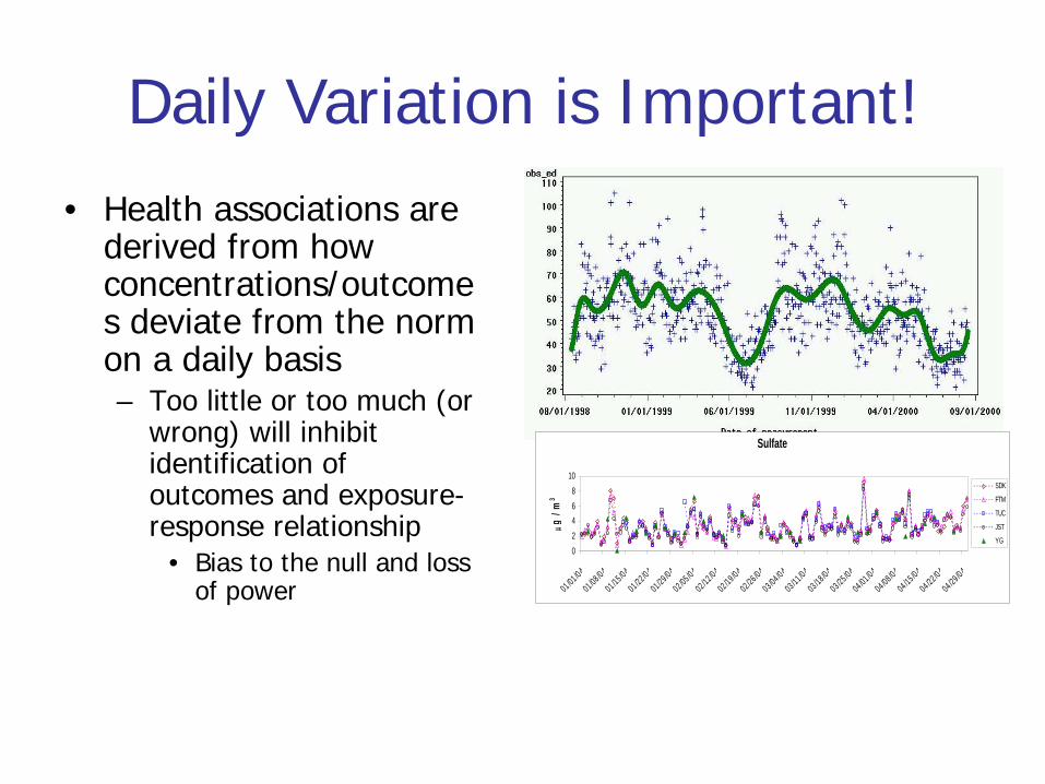
Daily Variation is Important!• Health associations are

derived from how concentrations/outcome s deviate from the norm on a daily basis– Too little or too much (or

wrong) will inhibit identification of outcomes and exposure- response relationship

• Bias to the null and loss of power

Sulfate

02468

1001 /01 /0401 /08 /0401 /15 /0401 /22 /0 401 /29 /0 402 /05 /0 402 /12 /0 402 /19 /0 402 /26 /0 403 /04 /0 403 /11 /0 403 /18 /0403 /25 /0404 /01 /0404 /08 /0404 /15 /0404 /22 /0 404 /29 /0 4

μg /

m3

SDK

FTM

TUC

JST

YG

Cautionary notes on receptor and emissions-based air quality models

• Both approaches– Tend to agree relatively well on average – (usually) identify large vs. small sources

• Sometimes by their absence• Receptor models

– Methods, based on largely the same data, give different results• Significant uncertainties

– Gives more temporal variation in source impacts at a specific receptor site

• Too much? (reasons to think so)– Not apparent how to conduct thorough evaluation and uncertainty

analysis for all methods• Emissions-based models

– Propagate uncertainties in variety of inputs and process descriptions– Have less day-to-day variability (probably too little)

• Meteorological models and inventories do not capture temporal variability well

• May be more spatially representative– Can have obvious disagreements with the data

• At least we know there is a problem!

Application to Health Effects Associations

•

Used CMB-LGO and PMF*•

Applied in an emergency department time-series study (Rollins School of Public-Health, Emory University)

•

Relative Risks (RRs) associated with change in inter-quartile-range of 3-day moving averages of PM2.5 levels were estimated using Poisson generalized linear models.

* - Kim et al., Atm Env 38, 3349-3362, 2004

All respiratory (262 daily ED visits) Upper Respiratory Infection (161 daily ED visits)

0.90

0.95

1.00

1.05

1.10

Diesel

- PMF

Diesel

- CMB-LG

O

Gasoli

ne - P

MF

Gasoli

ne - C

MB-LGO

Mobile

- PMF

Mobile

- CMB-LG

O Zn Fe ECPM2.5 CO

Diesel

- PMF

Diesel

- CMB-LG

O

Gasoli

ne - P

MF

Gasoli

ne - C

MB-LGO

Mobile

- PMF

Mobile

- CMB-LG

O Zn Fe ECPM2.5 CO

Source-specific RRs: Mobile sources

All respiratory (263 daily ED visits) All cardiovascular (86 daily ED visits)

Diesel- PMF,CMB-LGO

Mobile- PMF

PM2.5CO

EC

FeGas- PMF

CO

Source-specific RRs: “Other” OC

0.90

0.95

1.00

1.05

1.10

1.15

1.20

Other O

C OCPM2.5

Gasoli

ne - P

MF

Other O

C OCPM2.5

Gasoli

ne - P

MF

Other O

C OCPM2.5

Gasoli

ne - P

MF

Other O

C OCPM2.5

Gasoli

ne - P

MF

Other O

C OCPM2.5

Gasoli

ne - P

MF

Other O

C OCPM2.5

Gasoli

ne - P

MF

Asthma/ Wheeze (54)

COPD (13) URI (161) Pneumonia(34)

All respiratory(263)

All CVD (86)

“Other” OC“Other” OC

“Other” OC

“Other” OC

“Othe

r”OC OC PM 2.5

Preliminary results… further analysis appears to reduce other OC association

Analysis of Area of Influence (AOI)

• To identify which sources or regions might impact a specific receptor

• Uses source based sensitivity and AOI to determine the spatial distribution of emission influences – Evaluate the impact of specific existing sources– Predict the impact of future sources

• Uses source based sensitivity fields to generate receptor- based sensitivity fields

• Method is based on the DDM-3D functionality in CMAQ• Computationally less intensive than adjoint modeling for

multiple receptors

AOI Development – Reverse Fields

• Using the complete set of forward sensitivities (at each point in the domain), receptor oriented fields can be computed at any point using an inverse transformation:

),(*, txs lkij

),,(* txxz rij

Forward sensitivity field for a source at k

Reverse sensitivity for receptor located at rx

),(*)() ,(1

*,

* txsxwtxxz l

N

kkijkrij ∑

=

=

AOI Development - Forward Fields/Back Inversion

1. Choose a receptor2. Calculate forward sensitivities of pollutants to emissions at 25 points & interpolation

3. Estimate backward sensitivities

4. Final AOI

Inversion

• The receptor based sensitivity field is known automatically after the interpolation

),(),( ,, txStxZ rkijkrij =

k1

Sk1

Z (k1 )

Forward Field k1 Influence of k1 on

k2

Sk2

Z (k2 )


k3

Sk3

Z (k3 )


k4

Sk4

Z (k4 )


AOI at

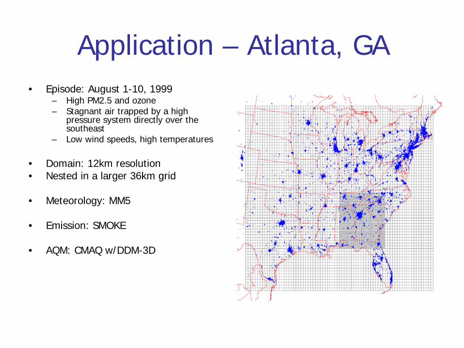
Application – Atlanta, GA• Episode: August 1-10, 1999

– High PM2.5 and ozone– Stagnant air trapped by a high

pressure system directly over the southeast

– Low wind speeds, high temperatures

• Domain: 12km resolution• Nested in a larger 36km grid

• Meteorology: MM5

• Emission: SMOKE

• AQM: CMAQ w/DDM-3D

Modeled PM2.5* Levels2.5

*Aitken and Accumulation Modes of Sulfate, Nitrate, Ammonium, EC, OC, and “unspecified”

Calculated Sensitivities

• Emissions– SO2

– NOX

– NH3

– anthropogenic VOC– elemental carbon

• Endpoint Pollutants– Total PM2.5

– Sulfate– Nitrate– Ammonium– EC– Anthropogenic SOA– Ozone

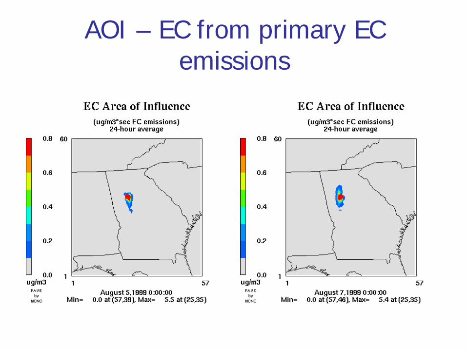
AOI – EC from primary EC emissions

AOI – Sulfate from SO2 Emissions

HYSPLIT Trajectories

Research Papers• Source apportionment of PM2.5 using different models

(A. Marmur, 2006; S. Lee, 2007; J. Baek, 2007)– CMAQ, CMB-MM, CMB-RG, CMB-LGO, PMF

• Improving emission inventories using tracer species (J. Baek, 2007)

• Regional source apportionment (S. Napelenok, 2006)• Improving emission inventories using inverse modeling

(S. Park, 2006; J. Baek, 2007; Y. Hu, 2007)• Area of influence (F. Habermacher, 2007; S. Napelenok,

2006, S. Kwon, 2007)• Use of SA results in Epidemiologic Studies (A. Marmur,

2006; J. Sarnet, 2006, 2007)

Summary• Sensitivity analysis based source apportionment fast

– Reduces numerical noise issues• No one source apportionment technique is a winner

– Too many reasons to list• Application of SA to epidemiologic studies has a number of model-

dependent issues– Capturing diurnal, day-to-day and spatial variability/representativeness

• Area of Influence (AOI) approach is a computationally effective method to get complete fields of both reverse and forward sensitivities– Extensible to other models and planning (prescribed fires)

• Inverse modeling using, metals, ions and EC/OC suggests major biases in inventories– Need to be investigated… don’t take as truth

Diesel Gasoline Road dust Wood burning

One issue:

Daily variation of fraction of major PM2.5 sources at JST

0

0.5

1

CM

AQ

0

0.5

1

CM

B-M

M

7/1/01 7/15/01 7/30/01 1/1/02 1/15/02 1/30/02

7/1/01 7/15/01 7/30/01 1/1/02 1/15/02 1/30/02

Inverse Modeling Using STN Tracer Species

Source apportionmentusing CMAQ

Source profiles Used in CMB

Tracer species concentration

Observations

Scaling factors

Improved CMAQ simulations

MultiplicationRegression analysis

obs

CMAQ

before

after

Quantitative Analysis: Regression analysis using tracer species

• Assumptions– Tracer species such as trace metals are non-reactive

and conservative in the atmosphere• Advantages

– Require less resources• Combined with CMAQ Tracer & DDM methods

– Site specific information– Source specific information

• Mobile sources: EC, OC and Zn• Wood combustion: K, EC• Road/soil dust: Al, Si, Ca

Regression analysis using tracer species – each species

• Representative tracers such as– EC– Silicon– Potassium– Zinc– Aluminum

• Can be used as a guideline to scaling factors of each source categories

integrated source/receptor- influence analysisintegrated source/receptor- based methods for source...

Documents