integrated status and effectiveness monitoring program (isemp) imws€¦ · ·...
TRANSCRIPT
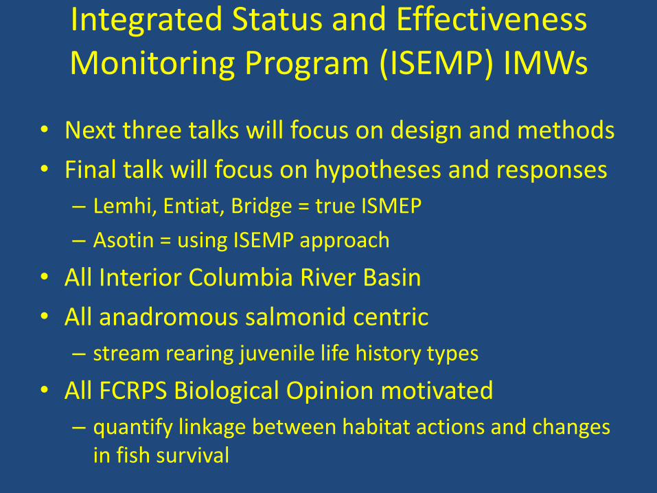
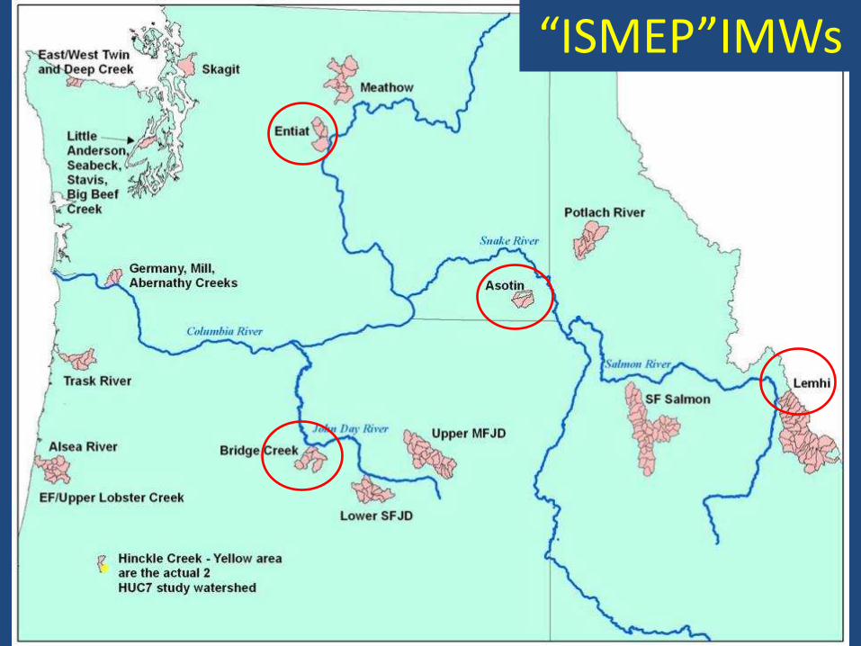
Integrated Status and Effectiveness Monitoring Program (ISEMP) IMWs
• Next three talks will focus on design and methods
• Final talk will focus on hypotheses and responses
– Lemhi, Entiat, Bridge = true ISMEP
– Asotin = using ISEMP approach
• All Interior Columbia River Basin
• All anadromous salmonid centric
– stream rearing juvenile life history types
• All FCRPS Biological Opinion motivated
– quantify linkage between habitat actions and changes in fish survival
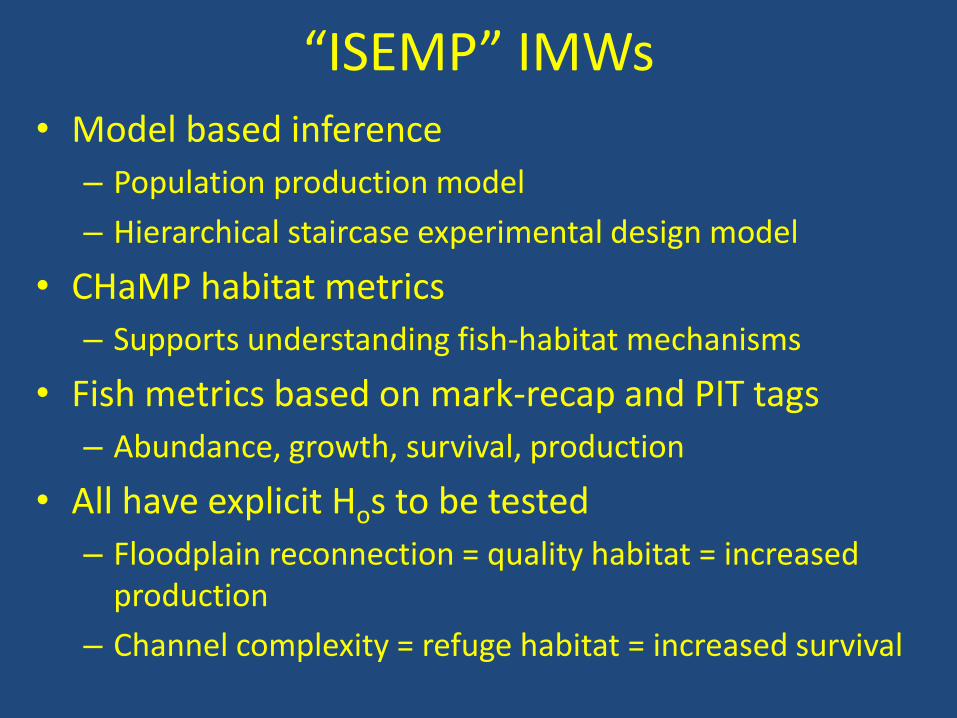
“ISEMP” IMWs • Model based inference
– Population production model
– Hierarchical staircase experimental design model
• CHaMP habitat metrics
– Supports understanding fish-habitat mechanisms
• Fish metrics based on mark-recap and PIT tags
– Abundance, growth, survival, production
• All have explicit Hos to be tested
– Floodplain reconnection = quality habitat = increased production
– Channel complexity = refuge habitat = increased survival

Watershed Production Model -Multi-Stage Beverton-Holt
where - N i,t = number of fish at life stage (i), time (t)
- Ni+1, t+1 = number of fish in next life-stage (i+1) and time (t+1)
- pi,t = productivity, or maximum survival rate for life-stage (i)
- c i,t = capacity, or maximum numbers that survive life-stage (i)
(Moussalli & Hilborn 1986)
ti
titi
ti
ti
Ncp
NN
,
,,
,
1,1 11
t
t
tSb
aSR
1
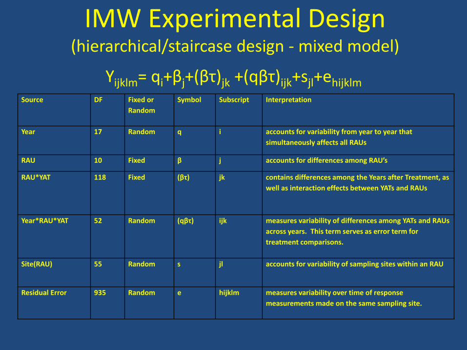
Yijklm= qi+βj+(βτ)jk +(qβτ)ijk+sjl+ehijklm Source DF Fixed or
Random
Symbol Subscript Interpretation
Year 17 Random q i accounts for variability from year to year that
simultaneously affects all RAUs
RAU 10 Fixed β j accounts for differences among RAU’s
RAU*YAT 118 Fixed (βτ) jk contains differences among the Years after Treatment, as
well as interaction effects between YATs and RAUs
Year*RAU*YAT 52 Random (qβτ) ijk measures variability of differences among YATs and RAUs
across years. This term serves as error term for
treatment comparisons.
Site(RAU) 55 Random s jl accounts for variability of sampling sites within an RAU
Residual Error 935 Random e hijklm measures variability over time of response
measurements made on the same sampling site.
IMW Experimental Design (hierarchical/staircase design - mixed model)
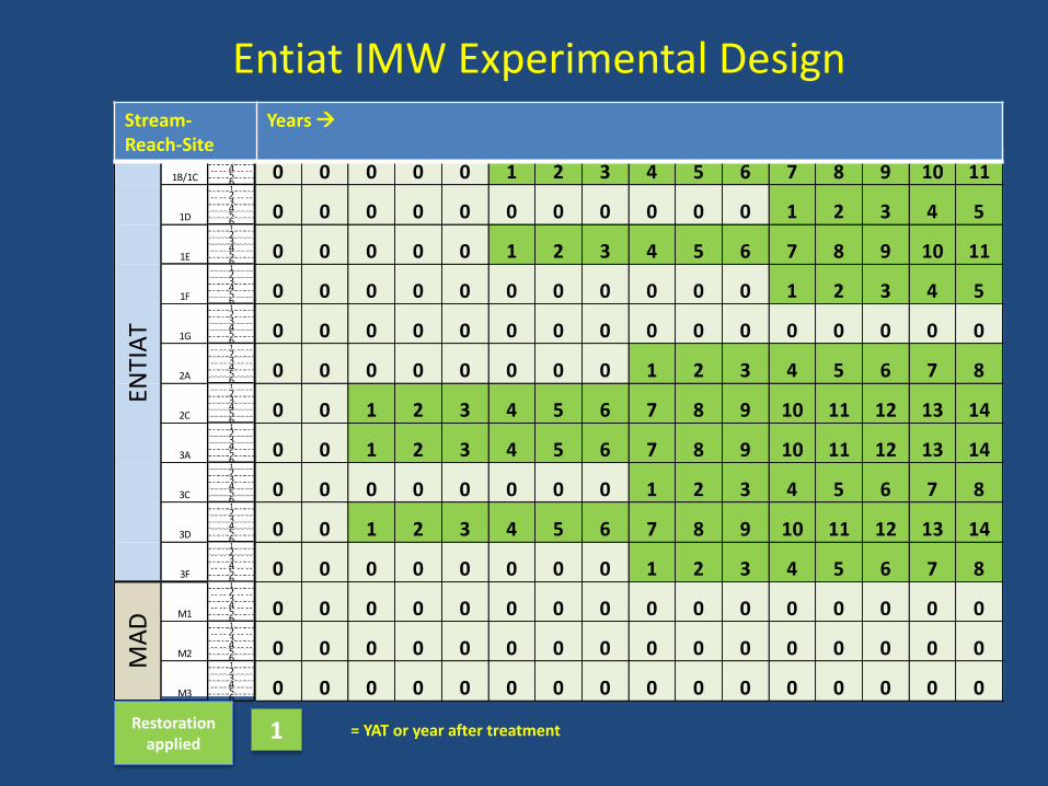
123456123456123456123456123456123456123456123456123456123456123456123456123456123456
1D
1E
1F
1G
2A
2C
3A
3C
1 2 3 4 5 6
10 11
1 2 3 4 5
3D
3F
MA
D M1
M2
M3
ENTI
AT
1B/1C
1 2 3 4 5 6 7 8 9
7 8 9 10 11
6
1 2 3 4 5 6
13
1 2 3 4 5 6 7 8 9
7 8 9 10 11 12
7 8 9 10 11 12
10 11 12
14
1 2 3 4 5
13
1 2 3 4 5
14
7 8
13
0
3 4 5 6
14
7 81 2 3 4 5 6
1 2 3 4 5 6 7 8
1 2
0
0 0 0 0 0
0 0 0 0
0 0 0 0 0 0 0 0 0 0 0 0 0
0 0 0 0 0
0 0 0 0 0
0 0 0 0 0
0 0
0
0 0 0 0 0
0 0
0 0
0 0
0 0
0 0
0 0
0 0
0 0
0 0 0 0 0 0
0 0 0
0 0 0 0 0 0
0 0 0 0 0 0
0
0 0 0 0 0 0
0 0 0
0 0 0
0 0 0 0 0
0 0 0 0 0 0 0 0 0 0 0 0 0 0
0 0 0 0 0
0 0 0 0 0
Restoration applied
1 = YAT or year after treatment
Entiat IMW Experimental Design Stream-Reach-Site
Years

“ISEMP” IMWs
• These four IMWs are not clones
• Common framework to support learning, but each has different rehabilitation methods and strengths
Intensively Monitored
Watersheds
“ISMEP”IMWs
Intensively Monitored
Watersheds
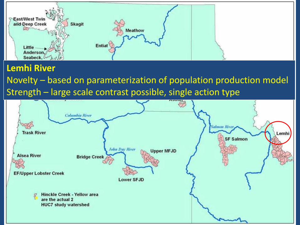
Lemhi River Novelty – based on parameterization of population production model Strength – large scale contrast possible, single action type
Intensively Monitored
Watersheds
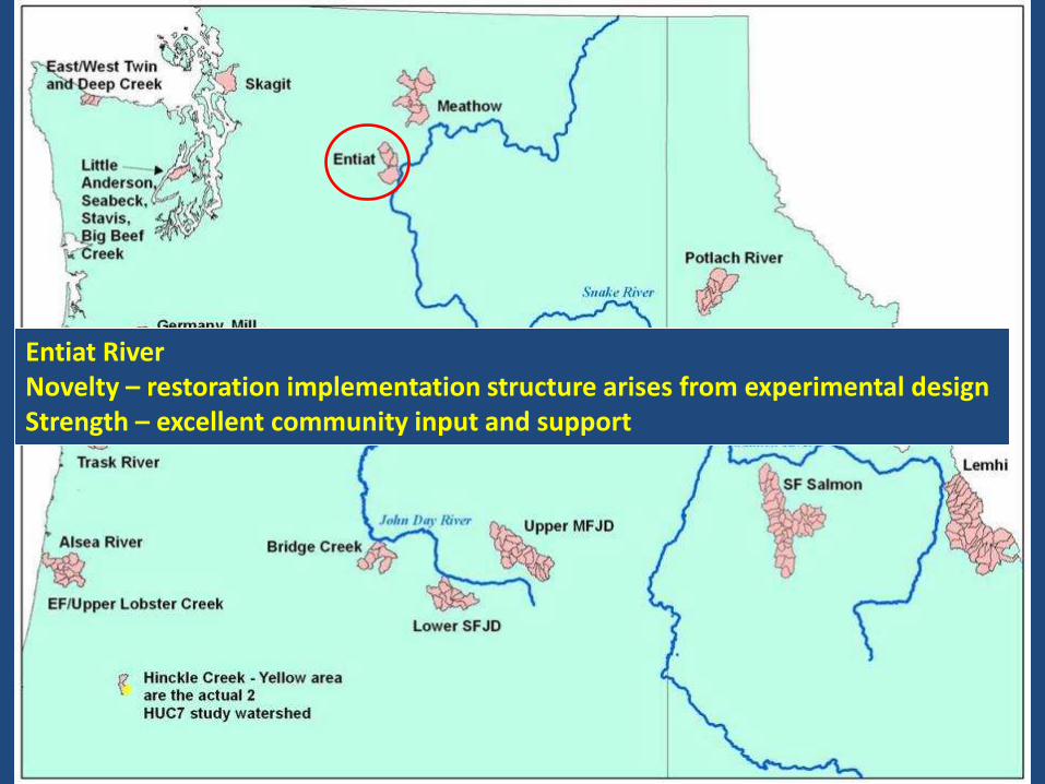
Entiat River Novelty – restoration implementation structure arises from experimental design Strength – excellent community input and support
Intensively Monitored
Watersheds
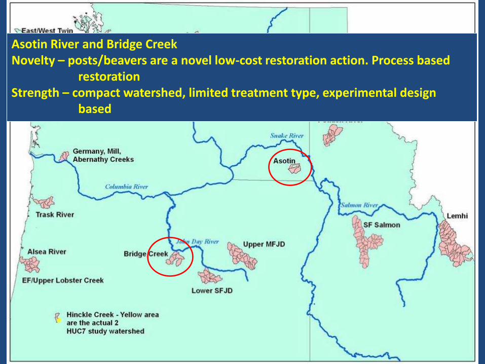
Asotin River and Bridge Creek Novelty – posts/beavers are a novel low-cost restoration action. Process based
restoration Strength – compact watershed, limited treatment type, experimental design
based

Data Management
• Common framework, including intentional contrast amongst “ISEMP” IMWs supports learning
• BUT – diversity of methods, participants, locations, large-scale/long term requires strong attention to
– Data Management
– QA/QC
– Storage/retrieval
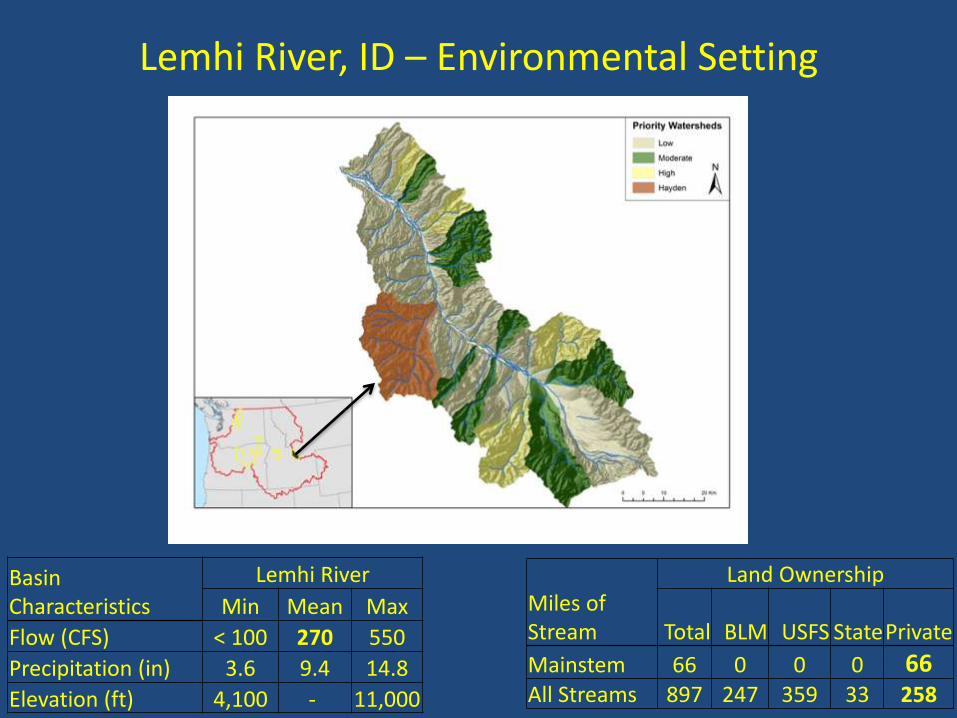
Lemhi River, ID – Environmental Setting
Miles of Stream
Land Ownership
Total BLM USFS State Private
Mainstem 66 0 0 0 66 All Streams 897 247 359 33 258
Basin Characteristics
Lemhi River
Min Mean Max
Flow (CFS) < 100 270 550
Precipitation (in) 3.6 9.4 14.8
Elevation (ft) 4,100 - 11,000

300+ diversions
1,500 cfs
Lemhi River Limiting Factors

Lemhi River Limiting Factors
Loss of Tributary Habitat
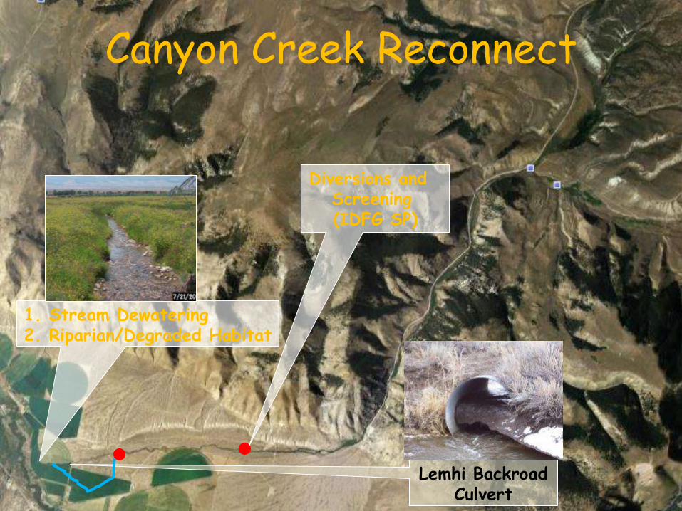
Canyon Creek Reconnect
1. Stream Dewatering 2. Riparian/Degraded Habitat
Diversions and Screening (IDFG SP)
Lemhi Backroad Culvert

LSC Reconnect Projects Flow Limited
L52 Removal (TNC/USBWP)
Little Spring Creek Rehab (TU)
Lower Diversion Removal (USBWP)
Fencing (IDFG/TU/USBWP)
Spring Creek/Pond Rehab (IDFG)
HWY 28 Culverts (USBWP)

Lemhi River – Assumptions
• Assumptions/Hypotheses:
– productivity limited by habitat quantity and quality
– life stage specific survival/abundance is a function of habitat quantity and quality
– those relationships can be modeled

Lemhi River - Watershed Model -Multi-Stage Beverton-Holt
where - N i,t = number of fish at life stage (i), time (t)
- Ni+1, t+1 = number of fish in next life-stage (i+1) and time (t+1)
- pi,t = productivity, or maximum survival rate for life-stage (i)
- c i,t = capacity, or maximum numbers that survive life-stage (i)
- Moussalli & Hilborn (1986)
ti
titi
ti
ti
Ncp
NN
,
,,
,
1,1 11
t
t
tSb
aSR
1
How to relate to habitat?
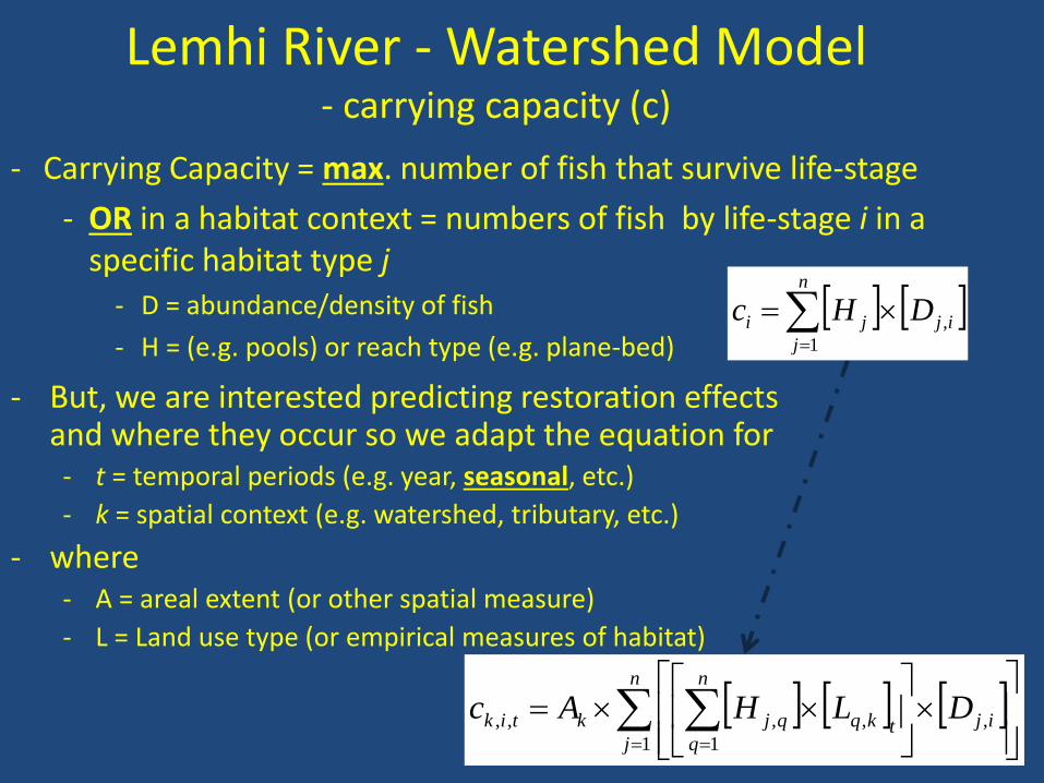
Lemhi River - Watershed Model - carrying capacity (c)
- Carrying Capacity = max. number of fish that survive life-stage
- OR in a habitat context = numbers of fish by life-stage i in a specific habitat type j
- D = abundance/density of fish
- H = (e.g. pools) or reach type (e.g. plane-bed)
- But, we are interested predicting restoration effects and where they occur so we adapt the equation for - t = temporal periods (e.g. year, seasonal, etc.)
- k = spatial context (e.g. watershed, tributary, etc.)
- where - A = areal extent (or other spatial measure)
- L = Land use type (or empirical measures of habitat)
ij
n
j
ji DHc ,
1
n
j
ij
n
qtkqqjktik DLHAc
1
,
1
,,,,

Lemhi River – Monitoring Approach • Information needs:
– adult escapement – brood-year specific juvenile abundance/survival in
tributary and mainstem habitat – habitat quantity/quality
• Response Design – LGD run decomposition via IPTDS – GRTS-distributed juvenile PIT tagging
• recap/re-sight via repeat surveys, IPTDS, and RSTs
– GRTS-distributed habitat sampling CHaMP – fish/habitat relationships described by
survival/abundance and contrast across tributaries
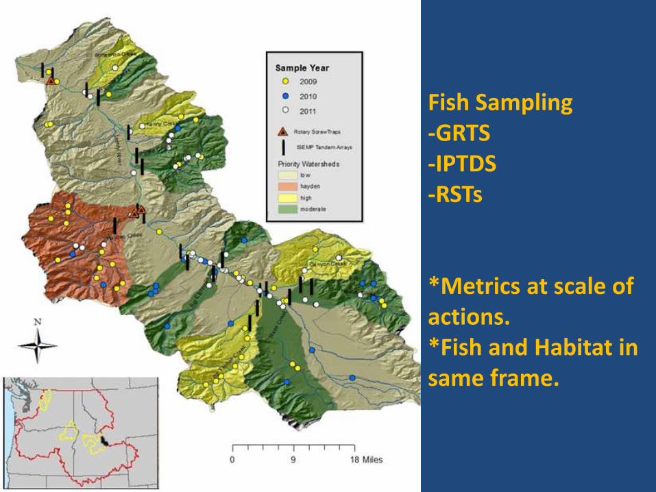
Fish Sampling -GRTS -IPTDS -RSTs *Metrics at scale of actions. *Fish and Habitat in same frame.
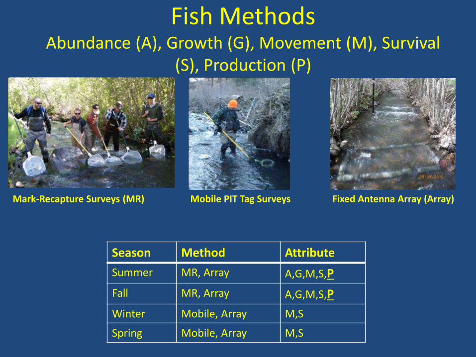
Fish Methods Abundance (A), Growth (G), Movement (M), Survival
(S), Production (P)
Mark-Recapture Surveys (MR) Mobile PIT Tag Surveys
Fixed Antenna Array (Array)
Season Method Attribute
Summer MR, Array A,G,M,S,P
Fall MR, Array A,G,M,S,P
Winter Mobile, Array M,S
Spring Mobile, Array M,S

Available Habitat: 285.1 km
LWD per km: 94.5 m3
Fine Sediment: 24.5 %
D50: 62.0 mm
Pool
Glide
Riffle
Mainstem Lemhi & Hayden
n = 40

Pool
Riffle Available Habitat: 23.4 km
LWD per km: 83.7 m3
Fine Sediment: 18.3 %
D50: 53.5 mm
Bohannon Creek
n = 2
Pool
Riffle
Glide
Available Habitat: 86.2 km
LWD per km: 24.7 m3
Fine Sediment: 26.6 %
D50: 22.3 mm
Kenny Creek
n = 3
Pool
Glide
Riffle Available Habitat: 64.0 km
LWD per km: 70.7 m3
Fine Sediment: 34.2 %
D50: 29.3 mm
Canyon Creek
n = 12
Pool
Glide
Riffle
Available Habitat: 103.0 km
LWD per km: 45.9 m3
Fine Sediment: 20.8 %
D50: 44.9 mm
Big Timber
n = 11
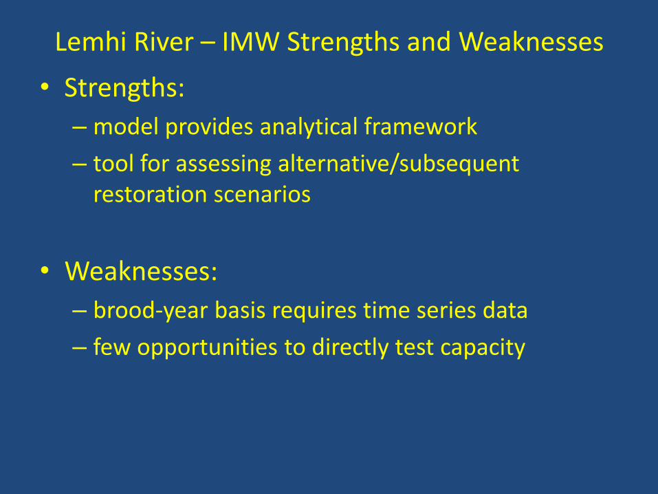
Lemhi River – IMW Strengths and Weaknesses
• Strengths:
– model provides analytical framework
– tool for assessing alternative/subsequent restoration scenarios
• Weaknesses:
– brood-year basis requires time series data
– few opportunities to directly test capacity
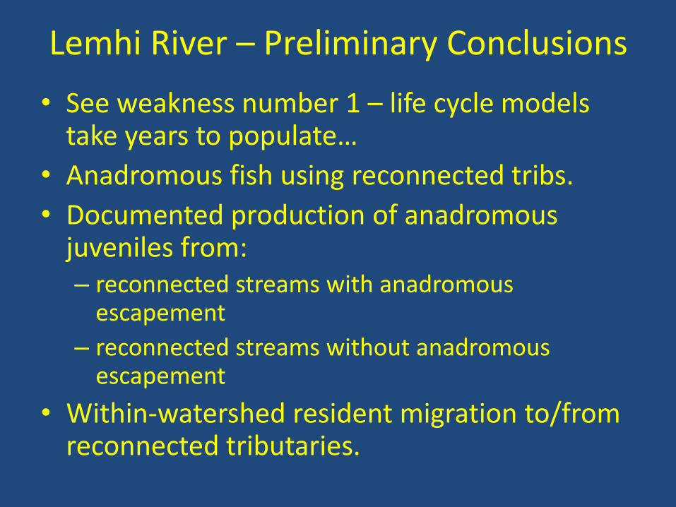
Lemhi River – Preliminary Conclusions
• See weakness number 1 – life cycle models take years to populate…
• Anadromous fish using reconnected tribs.
• Documented production of anadromous juveniles from: – reconnected streams with anadromous
escapement
– reconnected streams without anadromous escapement
• Within-watershed resident migration to/from reconnected tributaries.

Entiat IMW
Photo courtesy of Mike Cushman
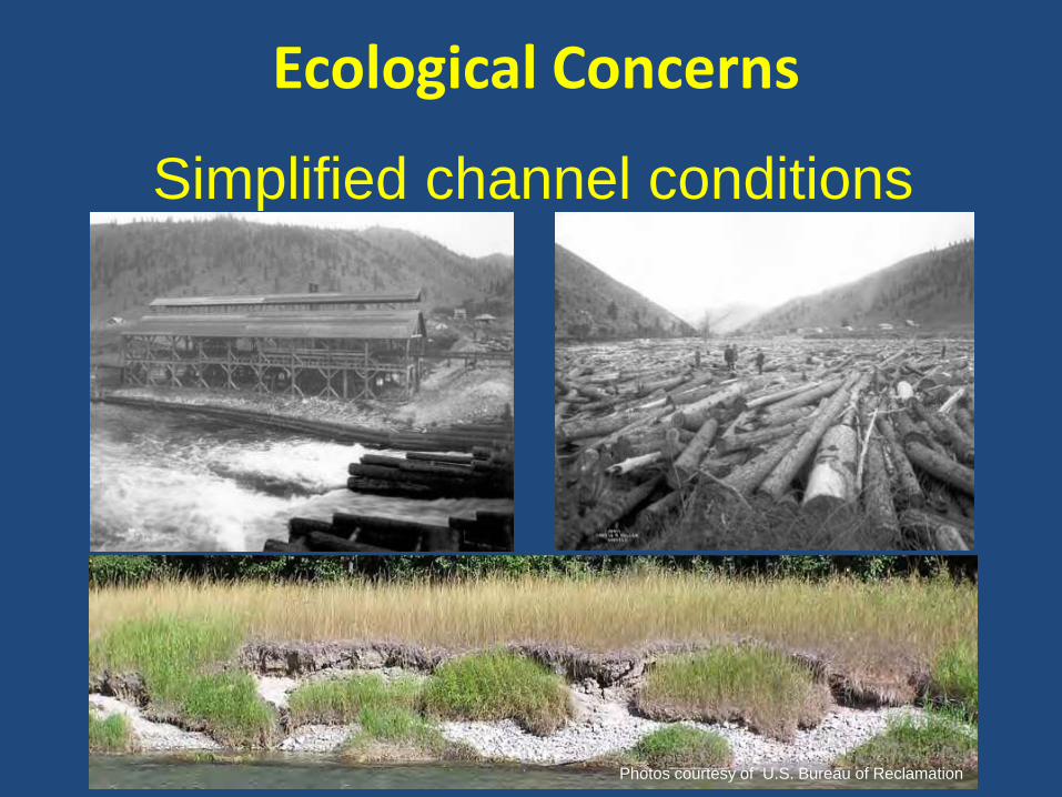
Ecological Concerns
Simplified channel conditions
Photos courtesy of U.S. Bureau of Reclamation
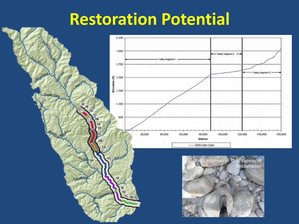
Restoration Potential
Photo courtesy of U.S. Bureau of
Reclamation

Entiat IMW Design
Valley Segment
Habitat Action Implementation Reach 2012
2014
2017
2020
VS3
3F
RM26
3E
3D
3C
3B
3A
VS2
2D
2C
2B
2A
VS1
1G
1F
1E
1D
1C
1B
1A
RM0
Temporary Control
Habitat Restoration Actions
No Identified Actions
Internal Control, never treated
Effectiveness Monitoring
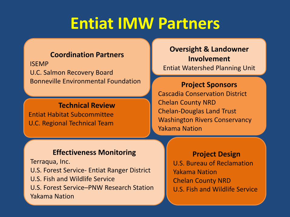
Terraqua, Inc. U.S. Forest Service- Entiat Ranger District U.S. Fish and Wildlife Service U.S. Forest Service–PNW Research Station Yakama Nation
Technical Review Entiat Habitat Subcommittee U.C. Regional Technical Team
Oversight & Landowner Involvement
Entiat Watershed Planning Unit
Project Design U.S. Bureau of Reclamation Yakama Nation Chelan County NRD U.S. Fish and Wildlife Service
Project Sponsors Cascadia Conservation District Chelan County NRD Chelan-Douglas Land Trust Washington Rivers Conservancy Yakama Nation
Coordination Partners ISEMP U.C. Salmon Recovery Board Bonneville Environmental Foundation
Entiat IMW Partners
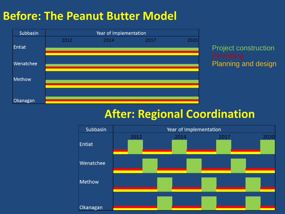
Before: The Peanut Butter Model
Planning and design Permitting Project construction
After: Regional Coordination
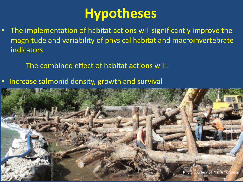
Photo courtesy of Yakama Nation
Hypotheses • The implementation of habitat actions will significantly improve the
magnitude and variability of physical habitat and macroinvertebrate indicators
The combined effect of habitat actions will:
• Increase salmonid density, growth and survival

Habitat Monitoring
Photo courtesy of Mike
Cushman
• Monitoring since
2005
• CHaMP since 2011
Channel Unit
Information
• Large wood
• Substrate type
• Undercut banks
• Fish cover
Site Information
• Total Drift Biomass
• Riparian Structure
• Solar Input
• Alkalinity
• Conductivity
• Temperature

Habitat Monitoring – Topographic Surveys
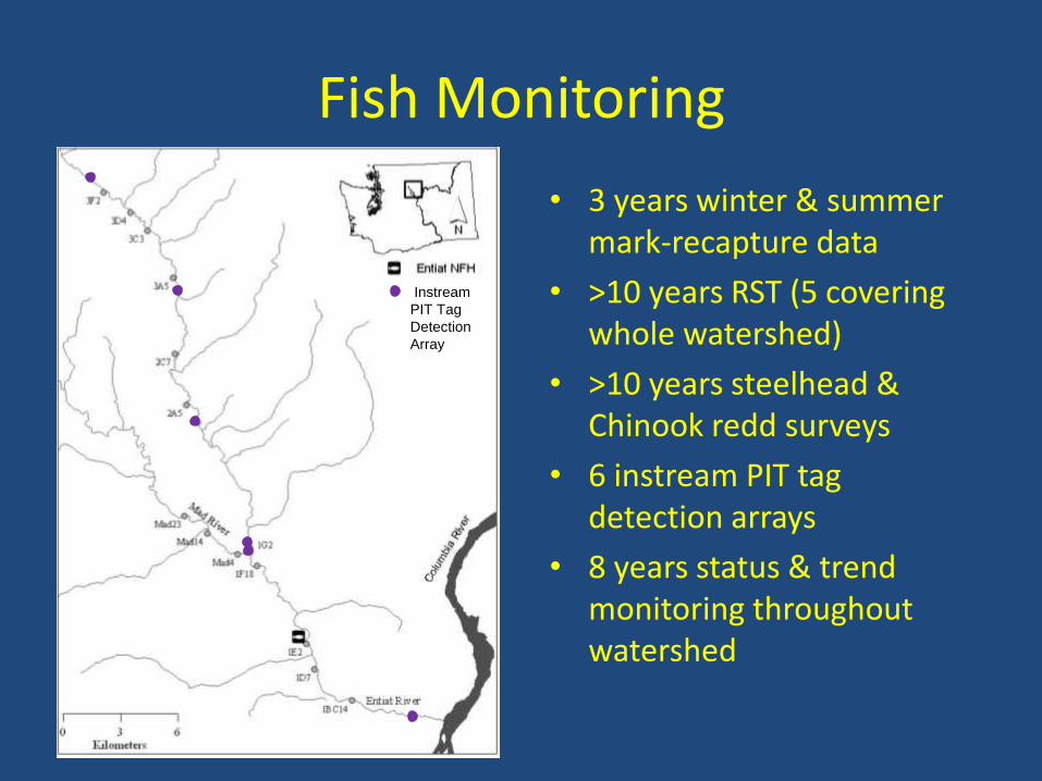
Fish Monitoring
• 3 years winter & summer mark-recapture data
• >10 years RST (5 covering whole watershed)
• >10 years steelhead & Chinook redd surveys
• 6 instream PIT tag detection arrays
• 8 years status & trend monitoring throughout watershed
IInstream
PIT Tag
Detection
Array

Strengths
• Community and collaborator support
• Well-coordinated effort
• Based on an experimental design with pulsed implementation – increase power to detect fish response
• Lots of monitoring

Challenges
• Limited restoration potential due to geomorphology and sociological constraints
• Massive coordination effort
• Access to private land
• Sampling large river
• Funding

Asotin Creek Intensively Monitored Watershed, southeast Washington
Presenter: Stephen Bennett Eco Logical Research Inc.
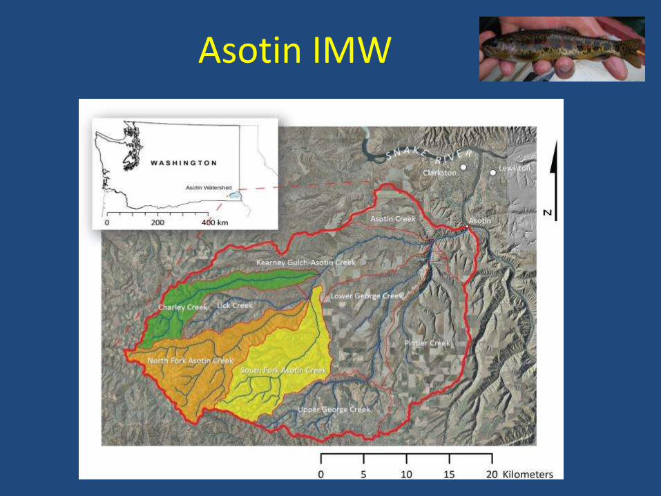
Asotin IMW
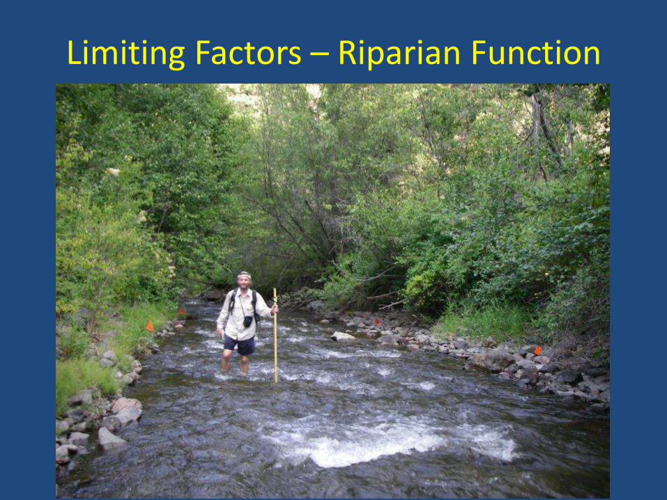
Limiting Factors – Riparian Function
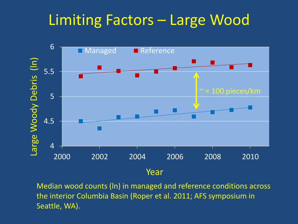
Limiting Factors – Large Wood
4
4.5
5
5.5
6
2000 2002 2004 2006 2008 2010
Managed Reference
Year
Larg
e W
oo
dy
Deb
ris
(ln
)
Median wood counts (ln) in managed and reference conditions across the interior Columbia Basin (Roper et al. 2011; AFS symposium in Seattle, WA).
~ = 100 pieces/km

Restoration Philosophy
• Let the River Do the Work (Zeedyk and Clothier 2009)
• Minimal impact
• Cheap and Transferable
• $100s/structure
• <10-15 m BFW (much of steelhead extent)
• Substitute density for stability
• 50 structures/km x 12 km = 600

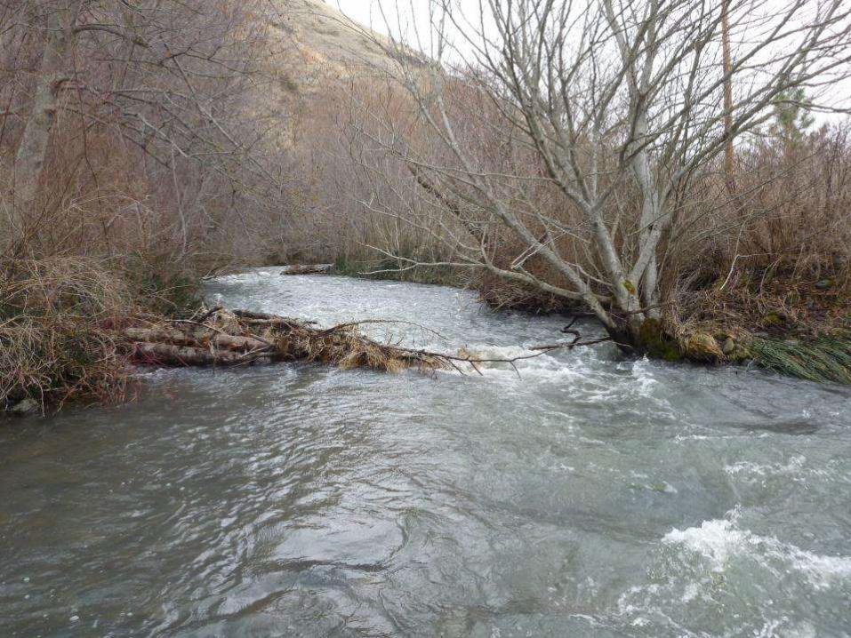
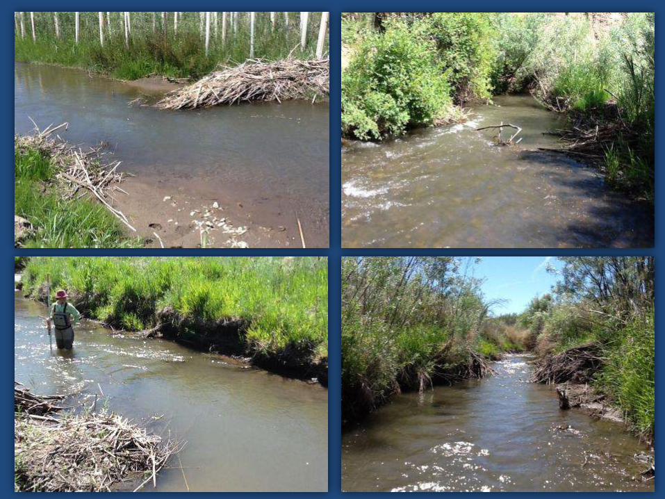
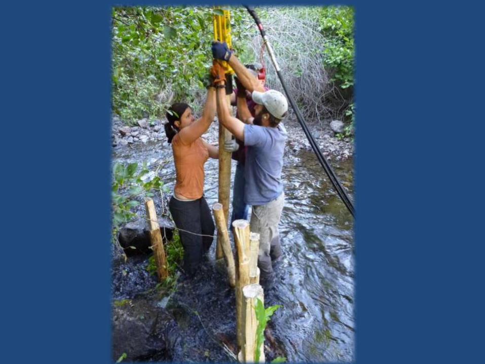
Restoration with PALS
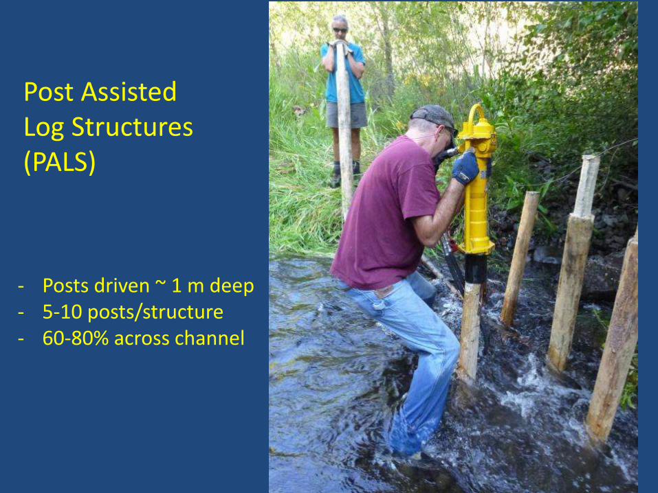
Post Assisted Log Structures (PALS)
- Posts driven ~ 1 m deep - 5-10 posts/structure - 60-80% across channel
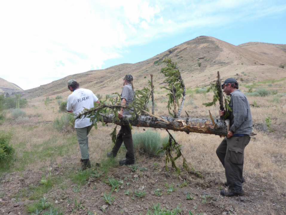

Posts - $20-50 LWD - donates (USFS) Labor - $50-150 $70-200
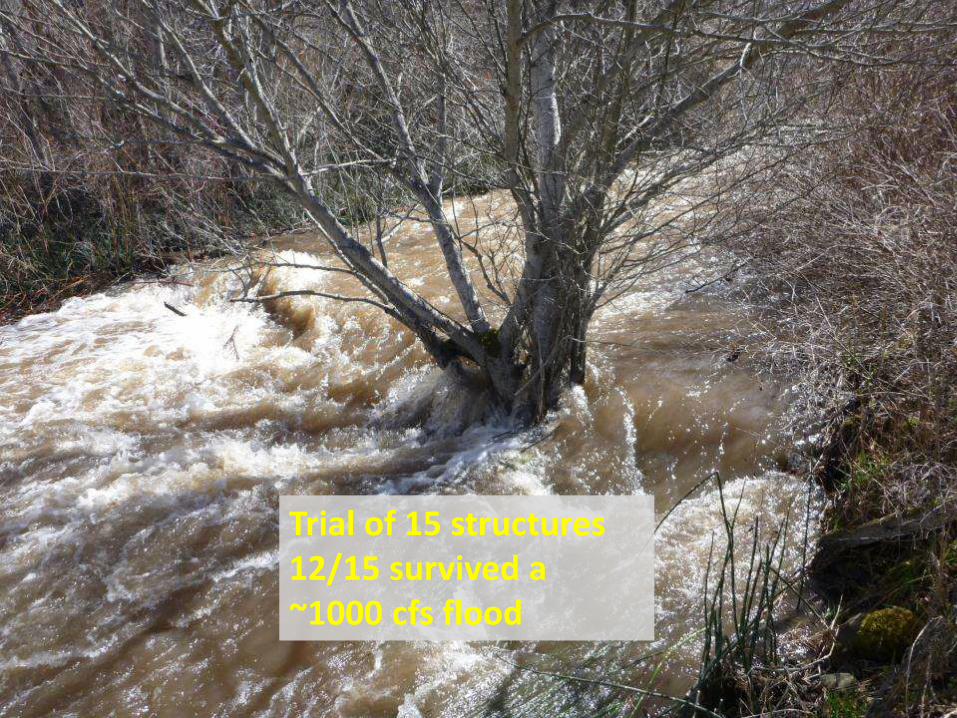
Trial of 15 structures 12/15 survived a ~1000 cfs flood
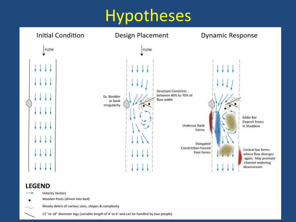
Hypotheses

Testing Habitat Hypotheses CHaMP Surveys
- DEM of Difference (DoD)
Pre-Treatment
Post-Treatment
= DoD
DEM = grid of x,y,z coordinates Using GIS Subtract “z” (elevation) for each x,y location Post – Pre treatment DEM = Change due to restoration Red = Erosion Blue = Deposition
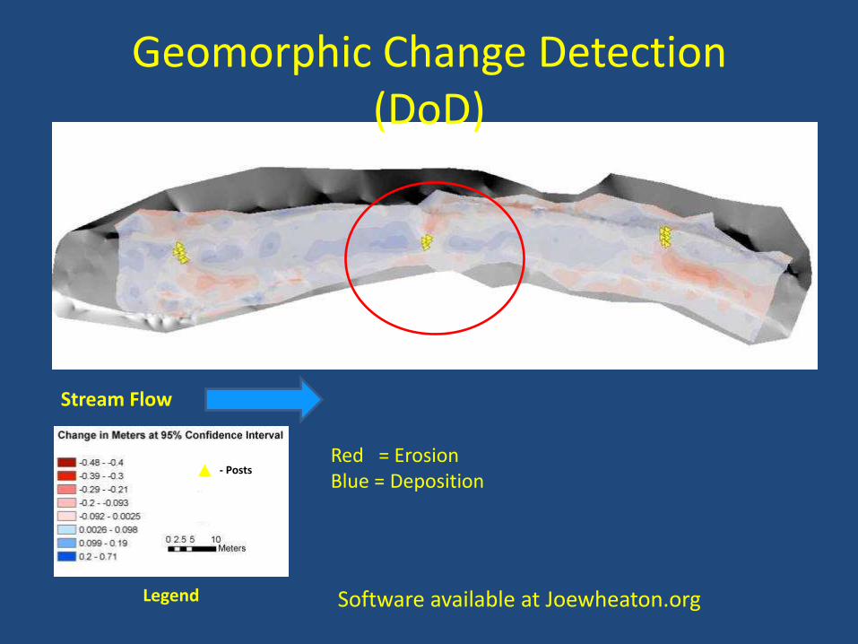
Stream Flow
Legend
- Posts
Geomorphic Change Detection (DoD)
Software available at Joewheaton.org
Red = Erosion Blue = Deposition

Experimental Design
Asotin Creek IMW experimental design. One treatment section will be treated each year starting in 2012. All other sections remain as controls.
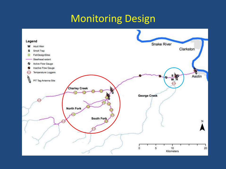
Monitoring Design

Fish Methods Abundance (A), Growth (G), Movement (M), Survival
(S), Production (P)
Mark-Recapture Surveys (MR) Mobile PIT Tag Surveys
Fixed Antenna Array (Array)
Season Method Attribute
Summer MR, Array A,G,M,S,P
Fall MR, Array A,G,M,S,P
Winter Mobile, Array M,S
Spring Mobile, Array M,S
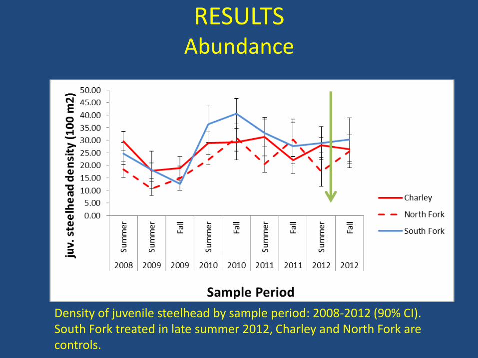
RESULTS Abundance
Density of juvenile steelhead by sample period: 2008-2012 (90% CI). South Fork treated in late summer 2012, Charley and North Fork are controls.

Conclusions
The Good
• Restoration approach feasible, cheap, effective, and highly transferable
• Design and Monitoring infrastructure robust – Ready to detect a change!
Not So Good
• Hard to keep time series going
• Funding Uncertainty

Acknowledgements Collaborators and Funding
Landowners and Sponsors
Thornton & Koch Families
Nick Bouwes and Nick Weber - Eco Logical Research, Inc., Providence, UT Joe Wheaton , Florie Consolati - Watershed Sciences, Utah State University, Logan, UT Chris Jordan, Michael Pollock, Jason Hall - NOAA Fisheries Service, Northwest Science Center Carol Volk- South Fork Research, Inc.
The ecological impacts of stream restoration: providing structures to assist beavers to aggrade an incised channel to
benefit endangered steelhead
Made possible by BPA and BLM

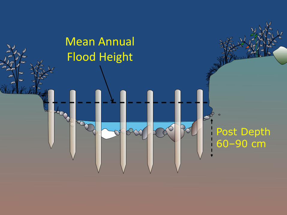
Mean Annual Flood Height
Post Depth 60–90 cm
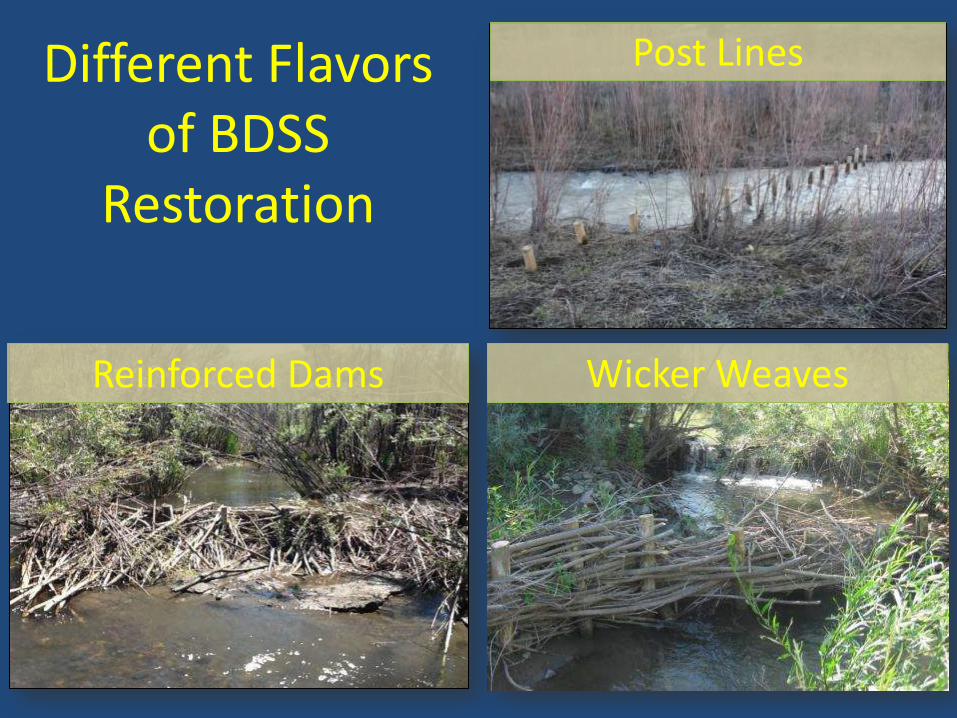
Different Flavors of BDSS
Restoration
Post Lines
Reinforced Dams Wicker Weaves

Beaver dam support structures
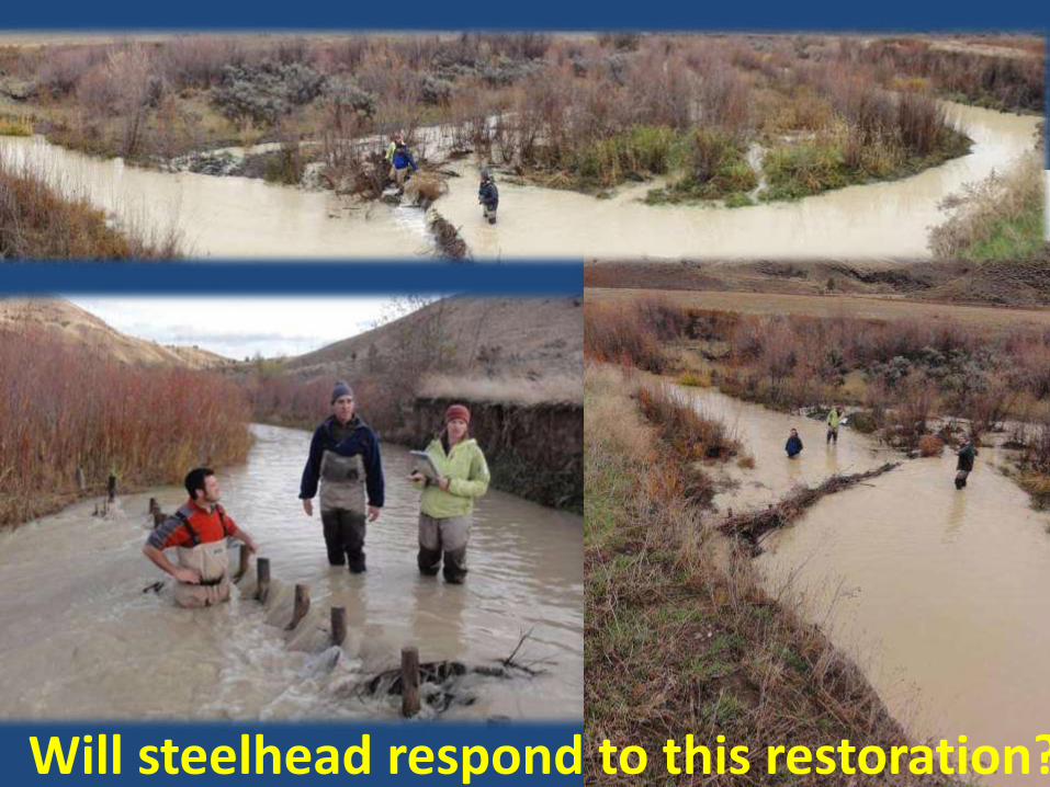
Will steelhead respond to this restoration?
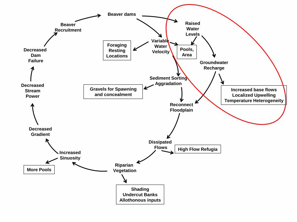
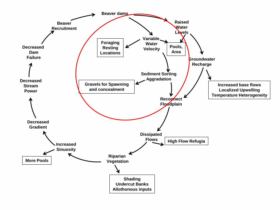
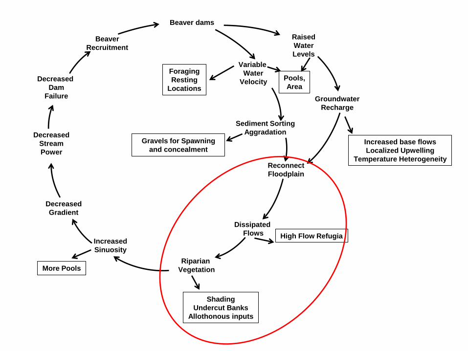
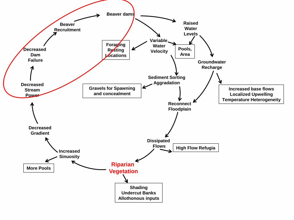
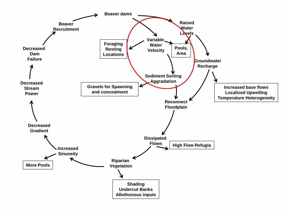
Beaver dams
Raised
Water
Levels
Variable
Water
Velocity
Sediment Sorting
Aggradation
Groundwater
Recharge
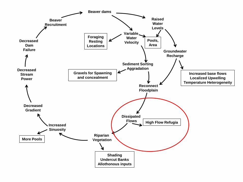
Reconnect
Floodplain
Pools,
Area
Dissipated
Flows Increased
Sinuosity
Decreased
Gradient
Beaver
Recruitment
Decreased
Dam
Failure
Decreased
Stream
Power
Increased base flows
Localized Upwelling
Temperature Heterogeneity
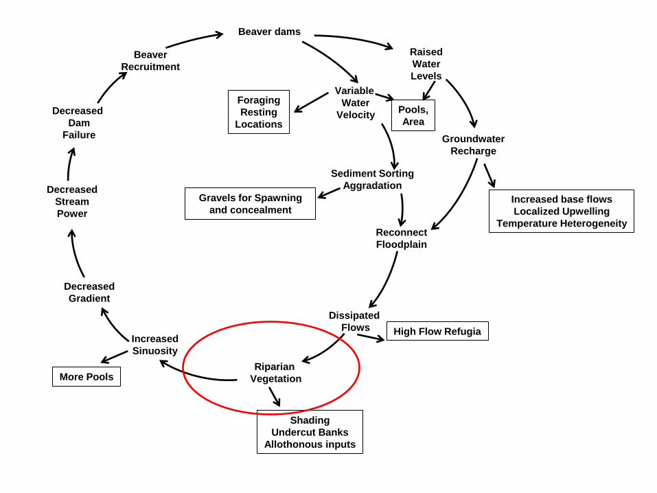
Riparian
Vegetation
Gravels for Spawning
and concealment
Foraging
Resting
Locations
High Flow Refugia
Shading
Undercut Banks
Allothonous inputs
More Pools
Beaver dams
Raised
Water
Levels
Variable
Water
Velocity
Sediment Sorting
Aggradation
Groundwater
Recharge
Reconnect
Floodplain
Pools,
Area
Dissipated
Flows Increased
Sinuosity
Decreased
Gradient
Beaver
Recruitment
Decreased
Dam
Failure
Decreased
Stream
Power
Increased base flows
Localized Upwelling
Temperature Heterogeneity
Riparian
Vegetation
Gravels for Spawning
and concealment
Foraging
Resting
Locations
High Flow Refugia
Shading
Undercut Banks
Allothonous inputs
More Pools

Expectations
More habitat (e.g. pools) More refugia (high flows, predators) More food More habitat complexity
Heterogeneity in: topography velocities temperature substrate
Increase in steelhead abundance, survival, growth and production
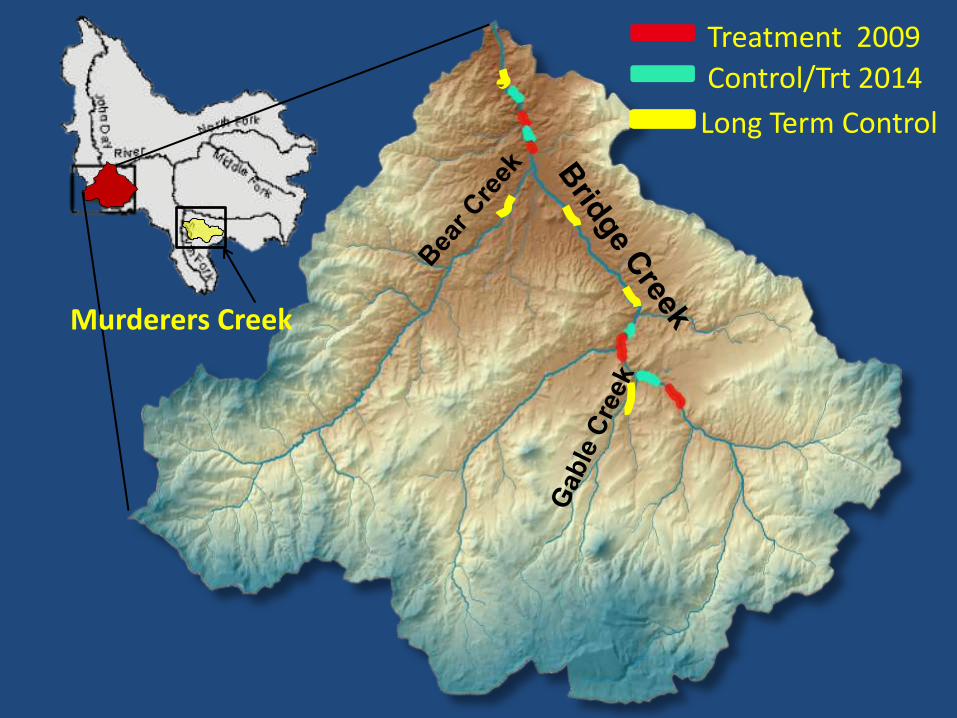
Treatment 2009
Control/Trt 2014
Long Term Control
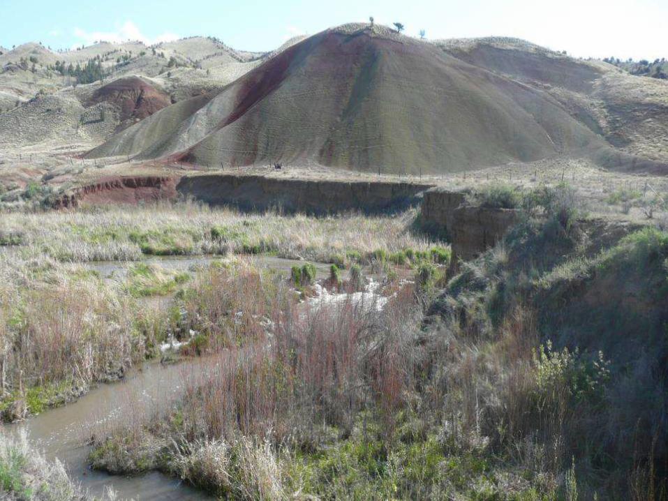
Murderers Creek
Beaver dams
Raised
Water
Levels
Variable
Water
Velocity
Sediment Sorting
Aggradation
Groundwater
Recharge
Reconnect
Floodplain
Pools,
Area
Dissipated
Flows Increased
Sinuosity
Decreased
Gradient
Beaver
Recruitment
Decreased
Dam
Failure
Decreased
Stream
Power
Increased base flows
Localized Upwelling
Temperature Heterogeneity
Riparian
Vegetation
Gravels for Spawning
and concealment
Foraging
Resting
Locations
High Flow Refugia
Shading
Undercut Banks
Allothonous inputs
More Pools
BDS Structure
DEM of Difference
Beaver dams
Raised
Water
Levels
Variable
Water
Velocity
Sediment Sorting
Aggradation
Groundwater
Recharge
Reconnect
Floodplain
Pools,
Area
Dissipated
Flows Increased
Sinuosity
Decreased
Gradient
Beaver
Recruitment
Decreased
Dam
Failure
Decreased
Stream
Power
Increased base flows
Localized Upwelling
Temperature Heterogeneity
Riparian
Vegetation
Gravels for Spawning
and concealment
Foraging
Resting
Locations
High Flow Refugia
Shading
Undercut Banks
Allothonous inputs
More Pools

Inset floodplain frequently inundated
Beaver dams
Raised
Water
Levels
Variable
Water
Velocity
Sediment Sorting
Aggradation
Groundwater
Recharge
Reconnect
Floodplain
Pools,
Area
Dissipated
Flows Increased
Sinuosity
Decreased
Gradient
Beaver
Recruitment
Decreased
Dam
Failure
Decreased
Stream
Power
Increased base flows
Localized Upwelling
Temperature Heterogeneity
Riparian
Vegetation
Gravels for Spawning
and concealment
Foraging
Resting
Locations
High Flow Refugia
Shading
Undercut Banks
Allothonous inputs
More Pools

What About the Fish?
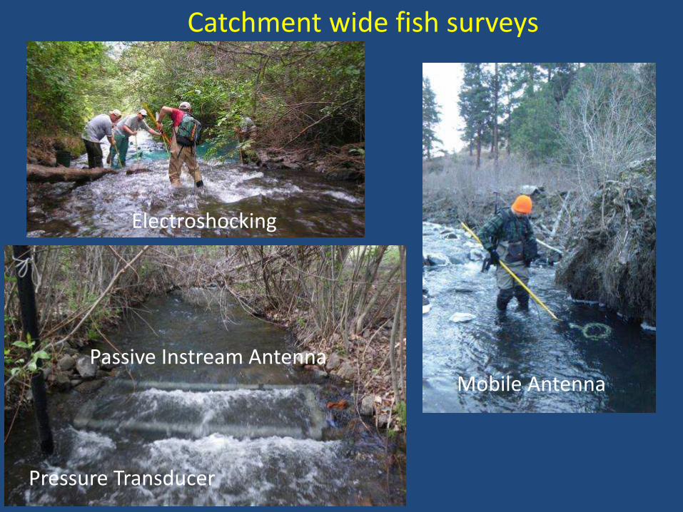
Passive Instream Antenna Mobile Antenna
Pressure Transducer
Catchment wide fish surveys
Electroshocking
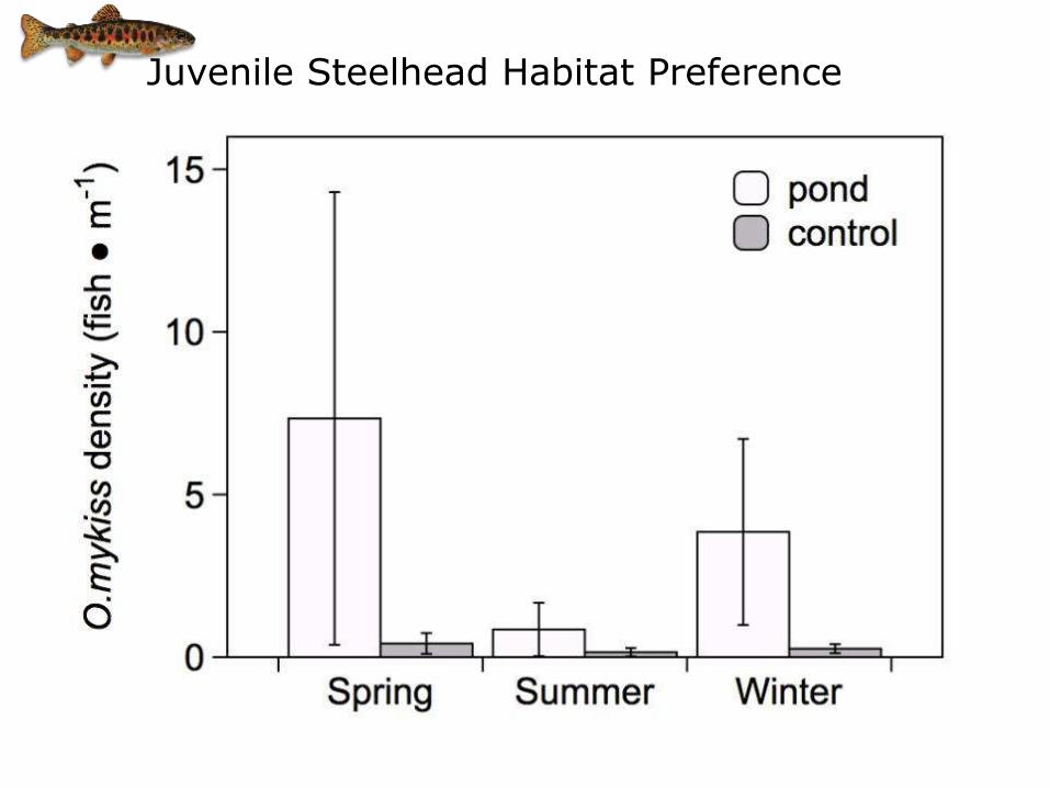
Juvenile Steelhead Habitat Preference
-20
0
20
40
60
80
100
120
Win
ter
Spri
ng
Fall
Win
ter
Spri
ng
Fall
Win
ter
Spri
ng
Fall
Win
ter
Spri
ng
Fall
Win
ter
Spri
ng
Fall
Win
ter
Spri
ng
Fall
O. m
ykis
s d
ensi
ty (
no
./1
00
m2)
Bridge (trt) Murderers (cntrl)
Pre-restoration Post-restoration
2007 2008 2009 2010 2011 2012
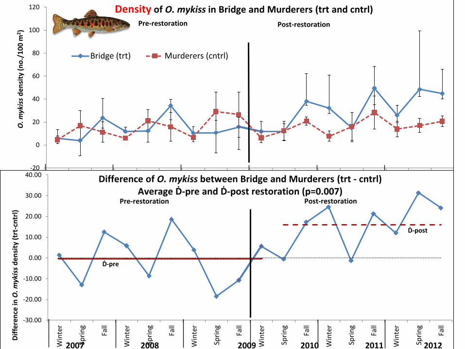
Density of O. mykiss in Bridge and Murderers (trt and cntrl)
-30.00
-20.00
-10.00
0.00
10.00
20.00
30.00
40.00
Win
ter
Spri
ng
Fall
Win
ter
Spri
ng
Fall
Win
ter
Spri
ng
Fall
Win
ter
Spri
ng
Fall
Win
ter
Spri
ng
Fall
Win
ter
Spri
ng
Fall
Dif
fere
nce
in O
. myk
iss
den
sity
(tr
t-cn
trl)
2007 2008 2009 2010 2011 2012
Difference of O. mykiss between Bridge and Murderers (trt - cntrl) Average Ḋ-pre and Ḋ-post restoration (p=0.007)
Pre-restoration Post-restoration
Ḋ-pre
Ḋ-post

0.00
0.20
0.40
0.60
0.80
1.00
1.20
Fall
Win
ter
Sum
mer
Fall
Win
ter
Sum
mer
Fall
Win
ter
Sum
mer
Fall
Win
ter
Sum
mer
Fall
Win
ter
O. m
ykis
s su
rviv
al s
eas
on
Bridge (trt) Murderers (cntrl)
Pre-restoration Post-restoration
2007 2008 2009 2010 2011 2012
Survival of O. mykiss in Bridge and Murderers (trt and cntrl)
0.00
0.20
0.40
0.60
0.80
1.00
1.20
1.40
1.60
Fall
Win
ter
Sum
mer
Fall
Win
ter
Sum
mer
Fall
Win
ter
Sum
mer
Fall
Win
ter
Sum
mer
Fall
Win
terR
atio
of
O.m
ykis
s su
rviv
al (
trt/
cntr
l)
2007 2008 2009 2010 2011 2012
Ratio of Survival O. mykiss in Bridge and Murderers (trt/cntrl) Geomean Ṙ-pre and Ṙ-post restoration (p<0.001)
Ṙ-pre
Ṙ-post
Pre-restoration Post-restoration
-5
0
5
10
15
20
25
30
35
40
Sum
me
r
Fall
Win
ter
Sum
me
r
Fall
Win
ter
Sum
mer
Fall
Win
ter
Sum
me
r
Fall
Win
ter
Sum
me
r
Fall
Win
ter
Sum
me
r
O. m
ykis
s gr
ow
th (
g/se
aso
n)
Bridge (trt) Murderers(cntrl)
2007 2008 2009 2010 2011 2012
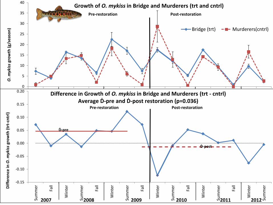
Growth of O. mykiss in Bridge and Murderers (trt and cntrl) Pre-restoration Post-restoration
-0.15
-0.10
-0.05
0.00
0.05
0.10
0.15
0.20
Sum
mer
Fall
Win
ter
Sum
mer
Fall
Win
ter
Sum
mer
Fall
Win
ter
Sum
mer
Fall
Win
ter
Sum
mer
Fall
Win
ter
Sum
merD
iffe
ren
ce in
O. m
ykis
s gr
ow
th (
trt-
cntr
l)
2007 2008 2009 2010 2011 2012
Difference in Growth of O. mykiss in Bridge and Murderers (trt - cntrl) Average Ḋ-pre and Ḋ-post restoration (p=0.036)
Ḋ-pre
Ḋ-post
Pre-restoration Post-restoration
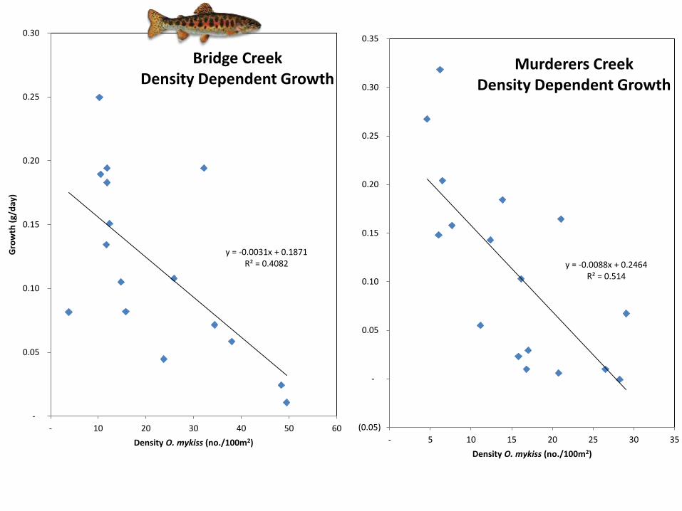
y = -0.0088x + 0.2464 R² = 0.514
(0.05)
-
0.05
0.10
0.15
0.20
0.25
0.30
0.35
- 5 10 15 20 25 30 35
Gro
wth
(g/
day
)
Density O. mykiss (no./100m2)
Murderers Creek Density Dependent Growth
y = -0.0031x + 0.1871 R² = 0.4082
-
0.05
0.10
0.15
0.20
0.25
0.30
- 10 20 30 40 50 60
Gro
wth
(g/
day
)
Density O. mykiss (no./100m2)
Bridge Creek Density Dependent Growth
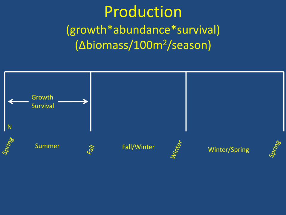
Production (growth*abundance*survival)
(Δbiomass/100m2/season)
Summer Fall/Winter Winter/Spring
Growth Survival
N

-50
0
50
100
150
200
250
300
350
400
450
Fall
Win
ter
Sum
me
r
Fall
Win
ter
Sum
me
r
Fall
Win
ter
Sum
me
r
Fall
Win
ter
Sum
me
r
Fall
Win
ter
Pro
du
ctio
n (
Δg/
10
0m
2/s
eas
on
) Bridge (trt) Murderers (cntrl)
2007 2008 2009 2010 2011 2012
Production of O. mykiss of Bridge and Murderers (trt and cntrl) Pre-restoration Post-restoration
-200
-100
0
100
200
300
400
Fall
Win
ter
Sum
mer
Fall
Win
ter
Sum
mer
Fall
Win
ter
Sum
mer
Fall
Win
ter
Sum
mer
Fall
Win
ter
Dif
fere
nce
in P
rod
uct
ion
(tr
t-cn
trl)
2007 2008 2009 2010 2011 2012 2012
Difference in Production of Bridge and Murderers (trt - cntrl) Average Ḋ-pre and Ḋ-post restoration (p=0.10)
Ḋ-pre
Ḋ-post
Pre-restoration Post-restoration
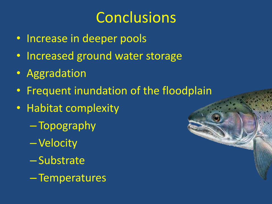
Conclusions • Increase in deeper pools
• Increased ground water storage
• Aggradation
• Frequent inundation of the floodplain
• Habitat complexity
– Topography
–Velocity
– Substrate
– Temperatures
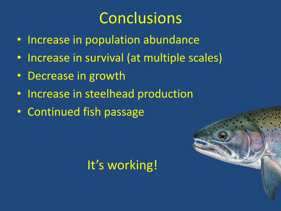
Conclusions • Increase in population abundance
• Increase in survival (at multiple scales)
• Decrease in growth
• Increase in steelhead production
• Continued fish passage
It’s working!