integrated supply chain design for sustainable and
TRANSCRIPT

INTEGRATED SUPPLY CHAIN DESIGN FOR SUSTAINABLE AND RESILIENTDEVELOPMENT OF BIOFUEL PRODUCTION
BY
YUN BAI
DISSERTATION
Submitted in partial fulfillment of the requirementsfor the degree of Doctor of Philosophy in Civil Engineering
in the Graduate College of theUniversity of Illinois at Urbana-Champaign, 2013
Urbana, Illinois
Doctoral Committee:
Professor Yanfeng Ouyang, ChairProfessor Imad L. Al-QadiProfessor Ximing CaiProfessor Madhu KhannaProfessor Jong-Shi Pang

ABSTRACT
The U.S. biofuel industry has been experiencing phenomenal growth during the last decade,
which may be partially attributed to the Energy Policy Act of 2005 and the Energy Inde-
pendence and Security Act of 2007. With such a sharp increase in biofuel demand, ethanol
manufacturing infrastructure must be significantly expanded. The booming industry can
have profound impacts on the economy, environment and society at national, regional and
local levels. It also imposes challenges to the existing infrastructure systems that support
the rapidly growing biofuel supply chain under the ethanol production mandate.
The economic feasibility and environmental sustainability of biofuel industry will be
highly dependent on the strategic design of the biomass-to-biofuel supply chain. Many
factors play important roles in the optimal design of a biofuel supply chain, such as the
regional geographical features (e.g., land and water resources), economic structure (e.g.,
availability, type and price of feedstock and energy), spatial distribution of demand, and
transportation infrastructure (network, modes and cost). They are also interdependent and
influenced by the configuration of a biofuel supply chain. As such, advanced decision tools
and systems analysis are in urgent need to provide viable strategies and design guidelines on
how biofuel production facilities and the supporting infrastructure should be expanded to
achieve the nation’s ambitious targets, and also insights into the potential economic, social,
and environmental impacts of the biofuel supply chain.
ii

We first review state of the art studies on biofuel development and its social economic
impacts, with a focus on transportation infrastructure, food versus fuel debate and farmland
use. We also discuss the competition between biofuel supply chain and the existing food
supply chain, as well as possible business scenarios between farmers and biofuel manufac-
turers. We then explore the various models developed for biofuel supply chain design and
biofuel logistics problems in existing literature, including statistical, simulation and opti-
mization models. For the theoretical and methodological literature that is closely related to
this problem, we review the classic facility location and supply chain design models and their
variations, such as the location equilibrium problem, network design problem, and the reli-
able facility location problem. We also briefly talk about some existing solution algorithms
to solve these optimization models.
The technical part of this dissertation starts with an integrated biofuel supply chain
model in which the shipment routing of both biomass feedstock and fuel product and the
resulting traffic congestion impact are incorporated to decide optimal locations of biofuel
refineries. A Lagrangian relaxation based heuristic algorithm is introduced to obtain near-
optimum feasible solutions efficiently. To further improve optimality, a branch-and-bound
framework (with linear programming relaxation and Lagrangian relaxation bounding proce-
dures) is developed. Numerical experiments are conducted to demonstrate that the proposed
algorithms solve the problem effectively. An empirical Illinois case study and a series of sen-
sitivity analyses are conducted to show the effects of highway congestion on refinery location
design and total system costs. We then build on this work to develop a more complex model
iii

by considering highway pavement rehabilitation decisions under pavement deterioration and
traffic user equilibrium with congestion in highway transportation networks. A reformulation
and iterative penalty method is applied to convert the bilevel network design problem into
a solvable single level mixed integer nonlinear program.
We further extended our models to account for uncertainties and risks in biofuel supply
chain design. We proposed a stochastic version of our supply chain design model that deals
with feedstock supply and ethanol demand uncertainties. From this model, the optimal sup-
ply chain configuration should well balance the trade-off between the expected operational
efficiency under uncertainties and the capital investment cost for building refineries. Monte
Carlo method is adopted to approximate the probabilistic distribution of spatial depen-
dent supply and demand and expected total system cost. Besides the feedstock supply and
ethanol demand uncertainties, bio-ethanol facilities and infrastructure are also susceptible
to disruption hazards. We further applies discrete and continuous reliable facility location
models to the design of reliable bio-ethanol supply chains for the State of Illinois (one of
the main biomass supply states in the U.S.) so that the system can hedge against potential
operational disruptions. The impacts of both site independent and dependent disruptions
are analyzed with a series of numerical experiments. Sensitivity analysis is also conducted to
show how refinery failure probabilities and penalty cost (for ethanol production reduction)
affect optimal supply chain configuration and the total expected system cost.
Another major issue that we address in this work is the allocation of farmland between
food and fuel productions, which has caused intensive concerns over food security and envi-
iv

ronmental sustainability. To this end, we develop game-theoretic models to find the optimal
design of a biofuel supply chain under farmers’ land use choice and feedstock market equi-
librium, and draw insights on different possible business partnerships between the biofuel
industry and farmers. To solve the game theoretic models, we develop a solution approach
that transforms the original discrete mathematical program with equilibrium constraints
(DC-MPEC) into to a solvable mixed integer quadratic programming (MIQP) problem. In
the last chapter, we further build on this work to analyze how possible governmental regula-
tions/policies on agricultural land use and greenhouse gas (GHG) emission would affect the
optimal biofuel supply chain design. We also develop two iterative relaxation algorithms to
solve larger scale DC-MPEC problem instances more effectively and efficiently.
In this work, a range of analytical approaches and customized solution algorithms (such as
Lagrangian relaxation, linear relaxation, branch and bound, reformulation, penalty method,
quasi-probabilistic method, and Monte-Carlo method) are developed to solve large-scale in-
stances of these models efficiently. The proposed models and solution algorithms are tested
in various empirical case studies, and the results not only provide insights on the potential
economic, social, and environmental impacts of the biofuel industry, but also provide guide-
lines for its sustainable development. The methodology framework can also be applied to
transportation planning and supply chain design problems in many other contexts.
v

Acknowledgements
I owe my deepest gratitude to my advisor, Professor Yanfeng Ouyang, for his tremendous
help in selection of the topic and in completion of the dissertation work. It was he who led me
into the field of operations research, provided me with the vision, and helped me with many
excellent ideas and advice throughout my graduate study. There have been ups and downs
in this process, but I could have not had any achievements on research without his support
and guidance. He has not only taught me the scientific knowledge, but also influenced me
with his passion and scientific rigor. I feel very fortunate to study under his guidance.
I would also like to thank the four other committee members, Professor Imad L. Al-Qadi,
Professor Ximing Cai, Professor Madhu Khanna and Professor Jong-Shi Pang, for spending
their time reviewing this work and providing valuable comments and suggestions. They
helped me expand my vision with their expertise in specific areas, and inspired me to come
up with some of the topics and research ideas in my dissertation. In particular, I would like
to thank Professor Jong-Shi Pang, who has collaborated with me on the last two technical
chapters in my dissertation, for contributing great ideas to this work on solving the highly
challenging problems.
vi

I am also grateful for the great opportunity I had to conduct research in the field of
transportation engineering. I would also like to express my thanks to all UIUC professors
from whom I have taken courses and learned knowledge. I would like to thank all my
former and current colleagues in my research group and my friends who have helped me in
both research and life, including Seungmo Kang, Xiaopeng Li, Fan Peng, Taesung Hwang,
Seyed Mohammad Nourbakhsh, Leila Hajibabai, Weijun Xie, Xin Wang, Yu-Ching Lee, etc.
Special thanks go to Seungmo Kang, Xiaopeng Li, Fan Peng, Taesung Hwang and Leila
Hajibabai, who collaborated with me on a number of research and course projects.
Finally, I would like to thank my family. They are my most important people, and it is
their love that supports me to finish my doctoral study.
This work is mainly supported by the US National Science Foundation through Grants
EFRI-RESIN #0835982. The Caterpillar Simulation Center at the University of Illinois
Research Park has also financially supported the last two semesters of my graduate study
at the University of Illinois.
vii

Contents
1 Introduction . . . . . . . . . . . . . . . . . . . . . . . . . . . . . . . . . . . . 1
2 Literature Review . . . . . . . . . . . . . . . . . . . . . . . . . . . . . . . . . 15
3 Biofuel Supply Chain Planning under Traffic Congestion . . . . . . . . . 32
4 Joint Optimization of Biofuel Supply Chain Design and Highway Pave-ment Rehabilitation Plan Under Traffic Equilibrium . . . . . . . . . . . . 59
5 Biofuel Supply Chain Design under Uncertainties and Risks . . . . . . . 82
6 Biofuel Supply Chain Design under Competitive Agricultural Land Useand Feedstock Market Equilibrium . . . . . . . . . . . . . . . . . . . . . . . 119
7 Biofuel Supply Chain Design under Farmland Use Regulations . . . . . . 142
8 Conclusions and Future Research Opportunities . . . . . . . . . . . . . . . 174
References . . . . . . . . . . . . . . . . . . . . . . . . . . . . . . . . . . . . . . . 182
Appendix A Proof for Propositions . . . . . . . . . . . . . . . . . . . . . . . . 193
viii
Chapter 1
Introduction
1.1 Motivation
As the need for alternative renewable energy continues to increase, the emerging biofuel in-
dustry in the U.S. has continued to boom as the nation aims to reduce transportation related
emissions and dependence on imported oils. Besides the domestic demand for alternatives
to high-priced foreign oil, a series of ambitious environmental policies provided remarkable
government support and subsidies, such as the Energy Independence and Security Act of
2007 (EISA) and the Food, Conservation, Energy Act (FCEA) of 2008. As such, the annual
production of ethanol from energy crops has grown from 200 million gallons in 1983 to about
13 billion gallons by the end of 2010. The congressional mandate EPA (2007) further requires
the annual production to reach 36 billion gallons by 2022, and over 80% of the mandated
increase is required to be based on cellulosic biomass feedstocks such as crop residues (e.g.,
corn stover) and dedicated energy crops (e.g., switchgrass and miscanthus). Corn starch-
based ethanol has become a significant energy source in the U.S. (Brown et al., 2007), while
1

new technologies are being developed for cellulosic biomass which is the so-called the “second
generation” of ethanol (US EPA, 2007).
Biofuel development is generally deemed as a promising way to enhance socio-economic
and environmental sustainability, however, such rapid development has far-reaching yet com-
plex impacts on critical issues such as food security for a growing global population. Massive
production of biofuel and related energy crops has already exerted impacts on the U.S. econ-
omy and the agriculture business modes. According to Oladosu et al. (2011) and IAPC
(2012), the share of corn being used for ethanol production has increased up to more than
40% in 2010 compared to only 10% in 2004/2005, and corn prices reached record high levels
in 2010/2011 that were more than 2.5 times higher than those in 2005. In observance of
the mandatory ethanol production requirement, this industry still has large room to grow
as the technology is advancing toward maturity. The ethanol manufacturing infrastructure
(particularly the cellulose-based ones) needs to be significantly expanded to provide suffi-
cient production capacity and ensure overall efficiency and reliability of the bioenergy supply
chain. These concerns impose great challenges to develop a sustainable supply chain system
that involves multiple interdependent stages (e.g., biomass production, harvesting, storage,
processing, and transportation) at regional, national or even global levels. Therefore, the
strategic design and planning for the biofuel supply chain system is particularly critical for
the long term commercial viability, and sustainability of the industry.
The biofuel supply chain design problem has several layers of decisions: number and
location of refineries, size of refineries, farmland allocation, supply scouring and demand
2
allocation, biomass and ethanol transportation, bio-product supply chain configuration etc.
Many factors play important roles in an optimal design, such as farmland and feedstock
price, ethanol demand, facility and labor cost, transportation infrastructure, water supply,
environmental concerns, as well as community resistance. These factors make the different
layers of decisions highly interdependent on each other, and thus highly complex to find an
optimal design of such a supply chain system.
1.1.1 Biorefinery Location and Traffic Congestion Impact
Biorefinery location decision is a key to the strategic bio-ethanol supply chain design.
It directly determines feedstock shipment and product (i.e., ethanol) distribution. Huge
capital investment is generally required to build a biorefinery plant, even for one with a
moderate size; for example, a corn-based biorefinery with a 100 MGY (million gallons per
year) capacity costs roughly $200 million (Swenson, 2008). As large biorefineries become
more and more popular, the investment in refinery construction constitutes a major portion
of the total supply chain cost.
One of the major operational costs in biofuel supply chain systems is from transporta-
tion of the bulky biomass feedstock (and ethanol), due to the low energy density of biomass
(especially cellulosic biomass such as miscanthus grass, switch grass, and corn stover) (Ja-
cobson et al. 2009). Moreover, transporting biomass and biofuel is concerned to worsen
the traffic congestion condition in the U.S. highway system which already has dramatically
increasing freight flows (Vedenov et al., 2010). The biofuel transportation cost in general
is proportional to the shipping distance, however, the large amount of heavy truck traffic
3
for biomass and biofuel can incur significantly higher transportation cost under severe traffic
congestions, and also social cost for public users due to excessive fuel consumption and travel
time. As such, biofuel logistics should be planned cautiously to minimize both its loss and
the social cost.
Furthermore, biomass transportation decisions (i.e., routing) should be considered en-
dogenously with refinery location decisions. On one hand, a large number of trucks must be
added to the highway network in order to ship sufficient low-energy-density biomass to satisfy
the enormous ethanol production requirement. The construction of biorefineries, therefore,
directly induces or diverts day-to-day traffic demand and alters the congestion pattern (and
hence transportation costs) in the network. On the other hand, the decision on refinery lo-
cations directly depends on the spatial distribution of biomass supply, ethanol consumption,
and the associated shipment costs. The congestion caused by biomass and ethanol shipment
may result in transportation cost increase and community resistance, which in turn are likely
to influence refinery location decisions. Hence, separating the decisions of bio-refinery lo-
cation and shipment routing and omitting the road congestion impact (especially in areas
with heavy background traffic) may not only cause unnecessary high transportation cost, but
also impose a negative socio-economic impact on the general public. As such, planning of
bio-refinery locations and biofuel logistics should be made cautiously for the long-run opera-
tions efficiency, in which the investment in refinery construction and operations, the cost for
biomass and ethanol transportation, and the related socio-economic impact are minimized.
4

1.1.2 Impact of Biofuel Supply Chain on both Traffic and Pave-ment Deterioration
As we just discussed, establishment of the new biofuel industry results in a booming
freight transportation demand for shipments between farms, refineries and gas stations. The
induced traffic, specifically heavy vehicle traffic, not only increases roadway congestion, but
also accelerates deterioration of pavement refineries.
Once refineries are constructed, most new transportation demands concentrate on espe-
cially the nearby local areas. Many of the existing local roads already do not have enough
capacity to accommodate the existing traffic loads. Therefore, the growth of biofuel indus-
tries potentially imposes pressure on highway operations and pavement quality, and may
result in damaged pavement conditions, more frequent rehabilitation activities (and more
user and agency costs), as well as thousands or millions of the existing individual road users
switching routes. As such, beyond just the direct congestion caused by the new traffic de-
mand for biofuel freight shipments as we discussed in chapter 3, there could be additional
congestion from travelers’ route changes due to highway maintenance and adverse pavement
condition.
The consequences could increase the public travel cost and lower the transportation
efficiency of the freight shipment, and the negative effect will in turn affect the optimal
refinery locations (Figure 1.1). These endogenous relationships have long been ignored in
the biofuel supply chain design literature. Therefore, the design of new large-scale biofuel
supply chains should simultaneously account for location of refineries, shipment routing
as well as the impacts on the highway networks. For maximum social benefit, pavement
5

infrastructure rehabilitation plans should be jointly optimized in the biofuel supply chain
design framework (i.e., refinery location, shipment routing) under traffic user equilibrium.
Figure 1.1: Interactions among refinery location, shipment and rehabilitation planning
1.1.3 Impact on Food Market and Farmland Use Implication
Large-scale production of energy crops has been impacting on the U.S. economy and
imposes challenges to resource supply systems that are associated with different stages of
the bio-fuel supply chain. In particular, the expected dramatic increase in U.S. biofuel
consumption induces new demand for bio-energy crops including first and second generations
of biomass. The new outlet for agricultural commodities results in competition between food
and energy use and as a result increases food prices. According to O’Brien and Woolverton
(2009), the U.S. average corn prices per bushel have increased dramatically since 2006, and
climbed up from $3.04 per bushel in the 2006/07 marketing year up to $4.20 during the
2007/08 marketing year. Biofuel production has been criticized for reducing food supply
and lifting up food prices to the record high in recent years (Rajagopal et al., 2009).
6

Figure 1.2: Demand and supply curve of corn under market equilibrium.
Regional agricultural pattern and feedstock market fluctuation should be integrated as
part of the biofuel supply chain design. The regional economic structure (e.g., availability,
type, and price of feedstocks, spatial distribution of supply and demand) not only affects
the biofuel supply chain design, but is also influenced by the supply chain configuration.
The massive expansion of the biofuel industry diverts a large amount of agricultural crops
as energy feedstocks, and in turn affects farmland allocation, feedstock market equilibrium,
and agricultural economic development in local areas. For example, in the advent of a new
biofuel refinery, farmers who used to ship corn to nearby local markets may be attracted to
sell corn as biofuel feedstock. As a result, the existence of biofuel refinery may boost local
corn price, resulting in higher cost on feedstock procurement (Mcnew and Griffith, 2005).
As such, having a large centralized refinery can decrease ethanol production costs through
economy of scale but may result in higher cost on feedstock procurement and production
distribution.
On the other hand, different business partnership that could be formed between farmers
7

and biofuel manufacturers also affect their investment decisions, individual profitability and
the welfare of the entire supply chain. In reality, farmers face a wide variety of risks such
as unforeseeable changes market prices. Although farmers can make operational decisions
each year, they also need to make long-term plan on whether to utilize their farmland to
grow crops or enroll part of their land in the Conservation Reserve Program (CRP), and
what types of crops to grow in the next few years. Given the high cost of building refineries,
transporting biomass feedstocks and inflexibility of changing farmland use, both farmers and
biofuel manufacturers would be interested in long-term contracts that ensure incentives for
farmers to grow sufficient feedstock supply and for manufacturers to invest on production
facilities (Keeney and Hertel, 2009). Hence, agricultural business modes should be integrated
as part of the biofuel supply chain design.
1.1.4 Risks and Uncertainties in Biofuel Supply System
The conventional biofuel supply chain design problem assume the input parameters (such
as bio-crop yield, demand and market price of ethanol) are deterministic, however, in reality
many stochastic factors could actually affect the operation of a biofuel supply chain. For
example, environmental condition could affect crop yield and then feedstock supply, while
policy changes and ethanol price fluctuation influence the local demand, etc. Due to these
uncertainties, a supply chain could to be designed robust enough to minimize the expected
total cost allowing for these potential fluctuations in resource supply and demand in the
system.
In addition, like many other facilities, bio-ethanol refineries are susceptible to disruption
8

hazards such as water scarcity, flooding, routine maintenance, or adverse weather condition
(Schill, 2008; Stillwater, 2002). Once refinery disruption happens, excessive operational cost
may occur due to the reallocation of biomass supply to more distant refineries. In addition,
huge gasoline price volatility and enormous societal cost (associated with producer or con-
sumer surplus) may be induced (Finizza, 2002). Therefore, in view of refinery disruption risk,
bio-ethanol supply chain design questions (e.g., how many and where to build biorefineries,
what sizes the refineries should be, and how to distribute feedstock to refineries) need to
be addressed systematically to develop economical, reliable and sustainable infrastructure
systems that are suitable for satisfying the mandatory future ethanol demand.
1.2 Objectives and Contributions
This Ph.D. research aims to develop comprehensive modeling frameworks for biofuel sup-
ply chain decision-making in a system level and spatial network scale. We focus on incorpo-
rating the interdependencies among infrastructure systems, and the social-economic impacts
of the emerging biofuel industry into an integrated supply chain design framework to pro-
vide guidelines for planners and policy makers to develop a sustainable and resilient biofuel
economy. Our studies will also provide a deeper understanding of the risks, uncertainties,
potential disruptive consequences in the biofuel supply chains.
In this dissertation work, we first review the recent studies on the key issues in biofuel
supply chain, and the classic supply chain models and their many variations, such as trans-
portation network models, user equilibrium, game theoretical models, location equilibrium
9

problems, as well as stochastic facility location problem. We then build upon the state-of-
art modeling approaches and solution techniques to develop innovative system optimization
models. We also develop customized solution algorithms which efficiently solve for optimal
solutions of the key decisions (e.g., refinery location, farmland/crop allocation). More impor-
tantly, we integrate important economic factors and social impacts into the network supply
chain system design problem. Our methodologies under different scenarios and concerns
provide insights on what are the best practices for the industry to establish a sustainable
supply chain maximizing the overall social benefit.
First, this study addresses the questions on (i) how the ever-growing shipment demand
from the booming bio-energy production industry may impose pressure on the existing trans-
portation systems, and (ii) how the biofuel production infrastructure should be expanded
so that the related negative social-economic impacts (e.g., traffic congestion) are minimized.
To the best of the authors’ knowledge, however, the bidirectional relationship between bio-
refinery location and biomass logistics has not been carefully studied. Specifically, the im-
pacts of biomass shipments on roadway congestion (and transportation costs) have been
generally ignored in the bio-energy supply chain design literature. To fill this gap, we for-
mulate an integrated mathematical model in which the shipment routing of both feedstock
and product and the resulting traffic congestion impact are incorporated to decide optimal
locations of biofuel refineries. Several custom-designed solution algorithms are proposed,
including a Lagrangian relaxation heuristic, a branch-and-bound algorithm with a linear
relaxation bounding, and a branch-and-bound algorithm with Lagrangian relaxation bound-
10

ing. Numerical experiments with several testing examples demonstrate that the proposed
algorithms solve the problem effectively. An empirical Illinois case study and a series of sen-
sitivity analyses are conducted to show the effects of highway congestion on refinery location
design and total system costs.
We continue to build on this model to address the relationship among biofuel supply chain
configuration, traffic equilibrium and pavement rehabilitation planning. The objective is to
build a more comprehensive integrated model to minimize the total system cost including the
transportation costs (for freight shipments and the public travelers) and infrastructure invest-
ments for both biofuel supply chain refineries and pavement rehabilitation activities. In our
modeling framework, realistic pavement performance models from the literature (Tsunokawa
and Schofer, 1994; Li and Madanat, 2002; Ouyang and Madanat, 2004) are used to account
for the impact of traffic on highway pavement refineries. The integration of refinery location,
shipment routing, and pavement rehabilitation makes the problem very challenging to solve.
The refinery location which involves integer variables is generally NP-hard, while pavement
rehabilitation models are highly non-linear. Besides, the bi-level nature of this problem (in
the form of NDP under UE) adds another layer of complexity. Given the hardness of this
problem, we develop an innovative solution algorithm that decomposes the original problem
into a series of solvable sub-problems, and effectively implement it on a hypothetical test
network. The Lagrangian relaxation algorithm is applied to separate the integer refinery
location variables, and the continuous bi-level sub-problem is further reformulated into an
equivalent single level model which can be solved in an iterative procedure.
11

We also extend our models to account for uncertainties and risks in biofuel supply chain
design. We proposed a stochastic version of our supply chain design model that deals with
feedstock supply and ethanol demand uncertainties. From this model, the optimal supply
chain configuration should well balance the trade-off between the expected operational ef-
ficiency under uncertainties and the capital investment cost for building refineries. Monte
Carlo method is adopted to approximate the probabilistic distribution of spatial dependent
supply and demand and expected total system cost by generating a large number of scenar-
ios. Our methodology is applied to a small test example and a series of numerical results are
discussed. Besides the feedstock supply and ethanol demand uncertainties, bio-ethanol facil-
ities and infrastructure are also susceptible to all kinds of disruption hazards, and the risk of
operation disruptions compromises the efficiency and reliability of the energy supply system.
We further applies discrete and continuous reliable facility location models to the design of
reliable bio-ethanol supply chains for the State of Illinois (one of the main biomass supply
states in the U.S.) so that the system can hedge against potential operational disruptions.
The discrete model is shown to be suitable for obtaining the exact optimality for small or
moderate instances, while the continuous model has superior computational tractability for
large-scale applications. The impacts of both site independent and dependent disruptions
are analyzed with a series of numerical experiments. Sensitivity analysis is also conducted to
show how refinery failure probabilities and penalty cost (for ethanol production reduction)
affect optimal supply chain configuration and the total expected system cost.
We further propose game-theoretic models that incorporate farmers’ decisions on land use
12

and market choice into the biofuel manufacturers’ supply chain design problem, including
a bilevel Stackelberg game and a single level cooperative game. The models determine
the optimal number and locations of biorefineries, the required prices for these refineries
to compete for feedstock resources, as well as farmers’ land use choices between food and
energy. Using corn as an example of feedstock crops, spatial market equilibrium is utilized to
model the relationship between corn supply and demand, and the associated price variations
in local grain markets. The proposed methodology is illustrated using an empirical case
study of the Illinois State. The computation results reveal interesting insights into optimal
land use strategies and supply chain design for the emerging “biofuel economy”.
The food versus fuel competition is essentially the competition for farmland. To model
the land competition under possible governmental regulation scenario for preserving food
production, we extend the Stackelberg game model to consider a cap-and-trade system sim-
ilar as that in the electricity market in Chen et al. (2011) and Zhao et al. (2010). In such
a cap-and-trade system, the government imposes an upper limit for the total land used
for growing energy crop in the entire supply chain network (i.e., to ensure minimum food
production) and allocates some free initial allowances for each farm. These allowances are
tradable among farmers with some additional benefit/cost (e.g., credits or trading price) for
every acre of land used for energy crops. Beside, given that commercial solvers would fail to
solve large scale instances of such a DC-MPEC model, we develop two customized iterative
relaxation algorithms with Lagrangian relaxation (LR) or linear program (LP) relaxation to
decompose and solve the problem. Our algorithms are shown to be a significant improvement
13

in terms of solving large scale DC-MPECs compared to the direct reformulation approach
that we developed earlier. Our numerical results provide insights into how such possible
governmental regulation/policy on agricultural land use and GHG emission would affect the
optimal biofuel supply chain design.
Although these studies focus on the biofuel production industry, the proposed method-
ologies can be easily generalized to be applied to other similar type of problem. For example,
our methodologies can be used to improve transportation planning and supply chain design
in other contexts (e.g., traffic impact studies for city planning). We can also adapt our model
to other emerging industries that encompass competitive effects with existing supply chains.
14

Chapter 2
Literature Review
This chapter reviews the existing models for biofuel supply chain design and biofuel logistics
problem including statistical, simulation and optimization models. We further explore the
state-of-art literature on social-economic impact of the rapid biofuel development, with a
focus on the fuel versus fuel debate and the impact on transportation infrastructure. We also
discuss the competition of the biofuel supply chain with existing food supply chain, farmland
use implication as well as possible business scenarios between farmers and manufacturers. For
the theoretical and methodological side of literature that is closely related to this problem,
we review the classic supply chain design models and their variations, including reliable
facility location problem under probabilistic disruptions, location equilibrium problems, and
network design problems.
15

2.1 Biofuel Supply Chain and Biomass Logistics Mod-
eling
In recent years, research has been conducted to address biomass logistics and biorefinery
location problems, using a variety of methodologies such as mathematical programming,
simulation, or Geographic Information System (GIS) based modeling. Sokhansanj et al.
(2006) built a dynamic integrated supply chain and logistics model to simulate the col-
lection, storage, and transport of agricultural biomass to a bio-refinery. The model uses
inter-connected discrete events and queues to simulate the entire network of material flow
from farms to a bio-refinery. The Western Bio-energy Assessment Team (2008) developed
an integrated model of biofuel supply chains by combining a spatially-explicit resource in-
ventory and assessment, biofuel production technologies, and transportation costs. They
used GIS with an infrastructure system cost optimization model to develop supply curves
of biomass feedstock throughout the western US. Other GIS-based optimization models
have also been developed to consider various factors such as feedstock availability, local bio-
fuel demand (Eathington and Swenson, 2007), or biomass prices variability (Panichelli and
Gnansounou, 2008). A multi-region, multi-period mixed integer mathematical programming
model was developed by Mapemba (2005) to determine the cost for delivering a steady flow
of lignocellulosic biomass feedstock to optimally located biorefineries. The bio-refinery lo-
cation problem has also been modeled as a discrete facility location problem and solved as
an integer-program. For example, Tursun et al. (2008) optimized the total cost includ-
ing transportation and processing of biomass, transportation of ethanol, capital investment
16

and operations for biorefineries. Kang et al. (2009) presented a multi-year supply chain
model for production of ethanol (both corn and cellulosic) and by-products. These studies
simply estimated transportation costs in the transportation network with the shortest path
distances.
Another group of studies focus on the cost effectiveness of biomass transportation through
competing modes. Kumar et al. (2006) proposed a multi-criteria assessment methodology
that integrates economic, social, environmental, and technical factors to rank alternatives
for biomass transportation. Several alternative transportation modes for biomass feedstock
and ethanol are evaluated in Searcy et al. (2007). A comprehensive comparison between
rail and truck reveals that railroad transportation is economical only when the shipment
distance exceeds 200 km (Mahmudi and Flynn, 2006). Due to the relatively higher cost
associated with shipping bulky feedstock biomass, it is generally recommended that biore-
fineries should be located near the source of biomass supply (normally within 80 km). Ku-
mar et al.(2006), Mahmudi and Flynn (2006) both analyzed the cost effectiveness of different
biomass transportation modes; the former proposed a multi-criteria assessment methodology
that integrates economic, social, environmental, and technical factors to rank alternatives
for biomass transportation, while the latter made a statistical comparison between rail and
truck transportation modes and found the economical distance for transshipment. With
similar statistical tools, Searcy et al. (2007) suggested that the optimal biorefinery location
should be close to the source of biomass rather than to the consumption point because of
the relatively high cost of moving feedstock.
17

2.2 Social Economic Impacts of Biofuel Supply Chain
2.2.1 Traffic Congestion and Challenges to Transportation Infras-tructure
Transporting biomass and biofuel is concerned to worsen the traffic congestion condition
in the U.S. highway system which already has increased freight flows (Vedenov et al., 2010).
Kang et al. (2010) suggests that truck as the major carrier for shipping biomass feedstock
to nearby refineries could lead to heavy traffic congestion and hence possible community
resistance. According to Ahmedov et al. (2009), the substantial increase of biomass and
biofuel transportation demand have affected traffic flows and in the U.S. highway network.
Their work evaluated the impact of biofuel energy policies, which mandated higher produc-
tion levels of biofuels, on grain transportation flows and the resulting traffic congestion in
the U.S. transportation network. In addition, Sexton and Zilberman (????) discussed an-
other indirect cause of traffic congestion due to biofuel production by reducing the price of
transportation fuel (by increasing supply) and increasing vehicle miles traveled by gasoline
consumers.
Trucking currently seems to be the most economical mode for biomass transportation.
While the growing biofuel industry may divert corn shipment traffic from export and feed
use, it is arguable that the diverted corn shipment traffic on highways is insignificant. First
of all, the majority of the future increase of ethanol production is from cellulosic biomass
(e.g., grass, corn stover). According to the 2007 EPA mandate, from 2007 to 2022 corn-
based ethanol will increase only 50% (from 10 billion gallon to 15 billion gallon) while
18
cellulosic ethanol will increase from zero to 22 billion gallons. As a result, the corresponding
shipment demand increase can be mainly attributed to the projected cellulosic biomass
(and ethanol) transportation, which is a net addition to the traffic in the highway network.
Furthermore, the cellulosic biomass is normally much bulkier than corn, hence it imposes
a much higher shipment demand (in terms of truckloads) than corn. In addition, existing
long-haul shipment of corn (for feed or export) are normally by rail or barge (Brown et al.,
2007), and hence the truck traffic diverted from corn export or feed use is likely to be of
minor significance. In addition, alternative transportation modes (e.g., barge, rail) would
require heavy investment in the infrastructure systems, because the existing systems are not
designed for (or readily available to) the emerging biofuel industry. For example, the current
pipeline infrastructure is not suitable for ethanol transportation due to erosion concerns.
2.2.2 Economic Impact of Biofuel Production
In view of the prospect of the biofuel industry, some researchers have raised concerns over
biofuel’s long-term socio-economic impacts including: e.g., the food-versus-fuel debate and
the new link between energy and agriculture markets (Chen et al., 2010; Johansson and Azar,
2007; Rajagopal et al., 2009; Walsh et al., 2003), the strategic changes in agricultural land
use (e.g., regular food crop production vs. Conservation Reserve Program (CRP) (USDA,
2011b)) and feedstock production (e.g., mix of feedstocks) required to support the biofuel
production goals (Khanna et al., 2008; Dicks et al., 2009), and the divergence between the
privately profitable and the socially optimal designs (Ervola and Lankoski, 2011). The food
versus fuel dilemma is essentially due to the limited resources (e.g., farmland). In other
19

words, the impact of biomass feedstock production on the food market is ultimately due to
the competition for farmland allocation between conventional food crops and energy crops.
Economic theories (e.g., partial and general equilibrium models) and simulation methods
have been used to estimate global and national impacts of the expanding biofuel industry
on macro-economic performance. For example, Rajagopal et al. (2009) and Chen et al.
(2010) examined the food-versus-biofuel trade-off in terms of losses and gains in consumer
surplus in different socio-economic sectors. Benjamin and Houee-Bigot (2007) focused on the
world arable crop markets and simulated the impact of alternative national and international
agriculture policies under land availability constraints using a partial equilibrium model.
Tyner and Taheripour (2008) conducted a firm-level ethanol refinery analysis and compared
break-even corn and ethanol prices under zero profit conditions. Rajagopal et al. (2009) built
a partial equilibrium multi-market framework to model the interactions between supply and
demand in food and fuel markets. In comparison, general equilibrium models capture the
economic implications at the global level rather than that at regional, industry or commodity
levels (e.g., Dicks et al. (2009); Feng and Babcock (2008); Gehlhar et al. (2010); Keeney and
Hertel (2009); Tyner and Taheripour (2008)). Simulation models were frequently utilized to
predict the growth of the ethanol industry with the gasoline/additives demand (Gallagher
et al., 2003), and bioenergy crop production and land use patterns under various agricultural
policies and bioenergy prices scenarios (Dicks et al., 2009; Walsh et al., 2003). The Biofuel
and Environment Policy Analysis Model (Chen et al., 2010) incorporated GHG emission and
social welfare implications to simulate market equilibrium for fuel, biofuel, food/feed crops
20

and livestock during 2007-2022.
These existing economic models, unfortunately, rely heavily on aggregated historical data,
but did not explicitly capture the mechanism behind the competition between the new bio-
fuel industry and existing food markets or the competitive behaviors of farmers, so they can
hardly provide useful insights in this regard (Tyner and Taheripour, 2008). While making
decisions on farmland allocation, refinery industry distribution, and ethanol production and
consumption (Berkes et al., 2003; Berkes and Seixas, 2005), state-of-the-art research on bio-
fuel supply chains generally adopts a sequential optimization approach to solve sub-problems
individually. For example, models for refinery planning generally assume that farmland use
and government regulations are already given. Similarly, it is a common practice to model
public agencies’ decisions assuming shipment demand from origins (e.g., farms) to destina-
tions (e.g., bio-refineries) are known (Meyer and Miller, 2001). These modeling approaches
unfortunately fail to address complex, dynamic interactions among various components of
the bio-energy supply chain.
2.2.3 Farmer and Manufacturer Partnership and Farmland UseImplication
While farmers and biofuel companies seek to maximize their own profits, factors such
as site-specific feedstock availability, price and transportation cost directly interrelate the
farmers’ decisions on farmland use to the industry’s decision on supply chain design.
On the other hand, different business partnership that could be formed between farmers
and biofuel manufacturers also affect their investment decisions, individual profitability and
21

the welfare of the entire supply chain. In reality, farmers face a wide variety of risks such as
unforeseeable changes in market prices. Although farmers can make operational decisions
each year, they also need to make long-term plans on whether to utilize their farmland
to grow crops or enroll in the CRP, and what types of crops to grow in the next few years
(Mapemba, 2005). Given the high cost of building refineries, transporting biomass feedstocks
and inflexibility of changing farmland use, both farmers and biofuel manufacturers would
be interested in long-term contracts that ensure incentives for farmers to grow sufficient
feedstock supply and for manufacturers to invest on production facilities (Larson et al.,
2008). (Mcnew and Griffith, 2005) developed a spatial econometric model to quantify the
local impact of introducing an ethanol plant on regional corn prices. Biofuel production was
found to push up crop prices, and therefore investing in refineries or contracting with biofuel
companies could also be beneficial to farmers. However, the existing studies are very relevant
but have not captured the economic behavior of buyers and sellers in local crop markets in
the biomass production models.
2.3 Supply Chain System Problems and Its Variations
2.3.1 Classic Facility Location Problem
The refinery location problems essentially fall into the general class of facility location
problems. Facility location studies can be traced back to its original formulation in 1909 and
the Weber Problem (Weber, 1957). Daskin (1995) have systematically introduced classic
discrete location models for deterministic problems. We review a one of the most relevant
22

facility location problem, the fixed charge facility location problems, mainly referring to
Daskin (1995). Fixed charge facility location problem balances the trade-off between one
time fixed cost for building facility and operating cost in order to minimize total system cost.
The one-time facility investment cost can be prorated over years or the long-term operating
cost can be aggregated to unify cost horizon. In this problems, facilities can be built at
locations in candidate set J to serve customers, and customer demand is distributed in a set
of nodes I and each i ∈ I generates λi units of demand. Let fj denote the unified one-time
building cost of a facility at j. The binary integer decision variables x = xjj∈J indicate
where to build facilities; i.e., a facility is built at j if xj = 1. Let dij denote the travel
distance from customer i to facility j. Auxiliary variables y = yiji∈I,j∈J is introduced,
where yij = 1 if customer i is served by facility j. The uncapacitated fixed charge facility
location (UFL) model can be formulated as follows:
minx,y
∑j∈J
fjxj +∑i∈I
∑j∈J
λidijyij, (2.1a)
subject to ∑j∈J
xj ≤ N, (2.1b)
∑j∈J
yij = 1,∀i ∈ I (2.1c)
yij ≤ xj,∀i ∈ I, j ∈ J , (2.1d)
xj ∈ 0, 1,∀j ∈ J , (2.1e)
23

yij = 0, 1, ∀i ∈ I, j ∈ J . (2.1f)
In this model, no more than N ≤ |J | facilities can be built in total due to the budget
constraint. The models (2.1) lay the foundation of many location models that have been used
in designing optimal supply chains. It can be extended in a variety of ways to deal with more
complex supply chain design problems. In complex supply chain systems, multiple stages of
service and interactions among facilities, and conflicting or competing objectives of the supply
chain participants may be incorporated into the fixed charge location model. Moreover,
detailed transportation routing can to be taken into account when the transportation cost
is significant.
2.3.2 Location-Equilibrium Problem, Network Design Problem andMathematical Programs with Equilibrium Constraints
The location-equilibrium problem was first proposed by Tobin and Friesz Tobin and
Friesz (1986) for locating a firm’s production facilities and determining production levels
while considering the impact on spatial equilibrium market prices. Variational inequalities
(Facchinei and Pang, 2003) were employed to model the competition among exiting firms
and new entrants, and the existence of equilibrium solution to these problems was proven
by Friesz et al. (1989). The location-equilibrium problem were further extended in Miller
et al. (1992a) by adding explicit product shipment variables, and a heuristic algorithm based
on sensitivity analysis methods was proposed. In contrast to previous papers where a large
locating firm enters a market with numerous price-taking small firms, Miller et al. (1992b)
24

considered the Stackelberg leader-follower oligopolistic competition and embedded the reac-
tion of Cournot firms into the location/production/shipping problem of the Stackelberg firm.
Other studies have considered multi-market oligopolistic spatial competition with heteroge-
neous production and logistics costs (Wu and Lin, 2003), alternative spatial pricing policies
(Hanjoul et al., 1990), and location and uniform pricing of new facilities (Aboolian et al.,
2008; Serra and Revelle, 1999). While some heuristic algorithms were described, the main
contributions of these early papers lie mainly in the identification of the applied problems
and their practical significance and in the formulation of mathematical programming models
for their subsequent study.
The rigorous analysis of the Stackelberg problem in the operations research literature,
including the development of efficient, provably convergent algorithms, did not begin until
the publication of the monograph Luo et al. (1996) that introduced the class of mathematical
programs with equilibrium constraints, abbreviated as MPECs. This monograph has inspired
a systematic investigation of the mathematical properties and solution algorithms for the
MPEC; this has resulted in a fairly advanced local theory based on standard nonlinear
programming on one hand and nonsmooth analysis on the other hand, and in a host of
computational algorithms for such problems. Several nonlinear programming solvers on the
neos site, such as filter, knitro, snopt, all have built-in functions to handle the special
equilibrium (mainly, complementarity) constraints that are the distinguished feature of an
MPEC and make this a challenging problem to solve.
Another school of research focuses on the network design problem (NDP) which de-
25

termines the optimal configuration of a network to achieve specified objectives, such as the
design of a transportation network, information network or supply chain network. This prob-
lem has long been recognized as a challenging one. Abdulaal and LeBlanc (1979) formulated
NDP with equilibrium constraints as an unconstrained non-linear optimization problem.
Yang and Bell (1998) reviewed variants of NDP models with multiple objective functions,
one of which accounts for the elasticity of travel demand by consumers. Some related al-
gorithms such as Iterative-Optimization-Assignment Algorithm, Link Usage Proportional
based Algorithm and Sensitivity Analysis-based Algorithm are also studied. Later, the same
authors proposed an equivalent single level problem to bi-level NDP by taking advantage of
the continuous and differentiable properties of the implicit user-equilibrium constraint. A
gap function was created, for which Augmented Lagrangian method can be employed to give
an exact local solution (Meng et al., 2001). Ban et al. (2006) further developed this idea by
transforming the lower level problem into a complementarity slackness condition for a single
level problem (Mathematical Programming with Complementarity Constraints, MPCC) and
used a Gauss-Seidel decomposition scheme to resolve the possible dimensionality issues. Lu
(2006) proposed an exact integer optimization formulation for network design problems un-
der User Equilibrium (UE) and deterministic travel demand; the non-linear model included a
quadratic objective, linear constraints, and mixed-integer optimization problem. Later, Shen
and Wynter (2011) proposed a single level convex optimization formulation to approximate
the bi-level structure; their method can be considered as a special case of the UE assignment
problem with elastic demand. Hence, it can be solved effectively using the standard path-
26

based traffic assignment algorithms (Shen and Wynter, 2011). In general, the NDP under
UE is a difficult problem because it is NP-hard in its general form (Johnson et al., 1978),
and it involves a large number of variables in many network contexts. Furthermore, it is
an instance of MPEC, which is a generalization of the bi-level optimization problem (Lu,
2006). The state of the art research mainly focuses on linear/quadratic program with linear
complementarity constraints (LP/QPCC) (Bai et al., 2011a; Hu et al., 2008, 2011a; Mitchell
et al., 2011). However, to the best of the authors’ knowledge, there are hardly any exact
algorithms that can efficiently solve MPEC with discrete variables (DC-MPEC), which the
NDP belongs to, especially for those involving nonlinear objectives/constraints.
2.3.3 Facility Location Problem under Uncertainties
The aforementioned models on biofuel supply chain all assume the parameters involved in
the design decisions deterministic, however, in reality many stochastic factors could actually
affect the design and operation of biofuel supply chain, such as, environmental factors that
affect bio-crop yield, farmland and crop prices, capital investment cost and transportation
cost, demand and market price of bio-ethanol, policy changes, etc. Due to these uncertainties,
a supply chain needs to be designed robust and flexible enough to achieve minimum expected
total cost in the uncertain environment. Literature has recognized the stochastic supply
chain design problems and developed many variations of the problem. Among them, supply
and demand uncertainties have been studied most extensively (Guillna et al., 2005; Schtz
et al., 2009). The decision on refinery locations directly depends on the spatial distribution
and quantity of biomass supply and ethanol consumption. The optimal refinery locations
27

should well balance between the expected operational efficiency under uncertainties and
the investment cost for building refineries. Therefore, the supply and demand uncertainties
should be considered to make refinery location and biomass transportation routing decisions.
MirHassani et al. (2000) applied scenario analysis and Benders decomposition for solving
a supply chain design problem under uncertain demand, and similarly Lucas et al. (2001)
applied scenario analysis and LR. Besides, Alonso-Ayuso et al. (2003) developed a branch-
and-fix algorithm to solve a problem with binary first-stage decisions and continuous second-
stage decisions.
2.3.3.1 Reliable Facility Location Problem under Disruptions
In deterministic and known settings, traditional facility location studies mainly focused on
efficiency and leanness of facility location design. However, it has been realized recently that
such “optimal” design may also be vulnerable to substantial operational risks from imperfect
information and underlying uncertainties (e.g., demand variations and facility disruptions).
Supply chain reliability and resilience against such risks have gained increasing attention.
Earlier literature examined facility congestion that arises from demand uncertainties and at-
tempted to enhance system availability by providing redundancy (Daskin, 1982, 1983; Ball
and Lin, 1993; Revelle and Hogan, 1989; Batta et al., 1989). After a series of devastating
disasters in recent years (e.g., 2005 Hurricane Katrina, 2003 U.S. Northeast blackout, 2008
China and 2009 Haiti Earthquakes), people have recognized the adversary impacts of poten-
tial disruptions on the supply side that may be caused by natural disasters, power outages,
operational incidents, labor actions or terrorist attacks. As a result, reliable facility location
28

models have been developed to design supply chains that can hedge against the impacts
of facility disruptions. Snyder and Daskin (2005) proposed a discrete integer programming
model for the reliable uncapacitated fixed charge location problem, assuming that facility
disruptions occur independently with equal probability. Cui et al. (2009) developed not
only a generalized discrete model to allow for site-dependent facility disruption probabili-
ties but also an alternative continuous model that significantly improves the computational
tractability. Li and Ouyang (2009) further generalized this continuous model to address
spatial correlations that may exist among facility disruptions. These models have also been
applied to deploy traffic surveillance sensors in highway and railroad networks (Ouyang et al.,
2009; Li and Ouyang, 2010a, 2010b). Compared with the traditional counterparts, the reli-
able models have significantly improved system reliability and reduced the expected overall
cost across normal and disruption scenarios.
2.3.4 Mathematical Modeling and Solution Approach
2.3.4.1 Lagrangian Relaxation
Discrete facility location problem including its variations mathematically belongs to the
category of mixed integer programming (MIP) problems. MIPs are generally difficult to
solve because of their intrinsic combinatorial complexity. LR-based approach, however, has
been proven to be powerful for separable integer programming problems and applied to
various supply chain design problems (Daskin, 1995; Li and Ouyang, 2011). Given a MIP,
the hard coupling constraints are first relaxed and put into the objective functions as a
penalty by the introduction of Lagrangian multipliers. The relaxed problem can then be
29

decomposed into subproblems (i.e., usually either continuous problems or simple integer
programs) which are relatively easier to solve. Multipliers are then iteratively adjusted
based on the levels of constraint violation. The dual function is maximized in this multiplier
updating process, and the values of the dual function serve as lower bounds to the optimal
feasible cost (Geoffrion and Graves, 1974). At termination of such updating iterations, simple
heuristics can be applied to adjust subproblem solutions to form a feasible result satisfying
all constraints. The subgradient method is commonly used to search for the optimal values
of dual variables, where the subgradient direction is obtained from the minimum solution
of the relaxed problem, and the multipliers are updated along this subgradient direction
(Zhao and Luh, 1998). As an effective decomposition method for solving facility location
and network design problems, LR will be extensively used throughout this dissertation to
solve different types of biofuel supply chain design problems.
2.3.4.2 MPEC
To date, MPEC is an established mathematical framework that has broad applications in
hierarchical decision making and optimal design. Particularly relevant to our research is the
linear/quadratic program with linear complementarity constraints (LP/QPCC) (Bai et al.,
2011a; Hu et al., 2008, 2011b; Mitchell et al., 2011), so is that with discrete design variables,
which the authors in Gabriel et al. (2010) and Garcia-Bertrand et al. (2006) have termed a
discretely-constrained (DC-)MPEC.
Most analytical achievements for solving the MPECs have been around the continuous
problems, including the group of developed commercial solvers. However, the DC-MPECs
30

have not been extensively studied in literature, and to date there is few approaches that
can efficiently solve such problems or is applicable to large scales problems. In a related
paper by Gabriel and Leuthold (2010), the authors introduced an MPEC formulation for
a network-constrained energy market. On one hand, under the boundedness of the deci-
sion variables, a DC-MPEC can be formulated as a mixed integer programming problem;
on the other hand, recent advances on the LP/QPCC have included the development of
specialized techniques such as branch-and-cut, logical Benders, disjunctive programming,
lift-and-relaxation, domain decomposition, and convexification of bilinearity to handle the
complementarity constraints. Therefore, one of the contributions of this dissertation work is
utilizing the existing theory of the LR algorithm and recent advances on MPECs to develop
a customized solution approach to solve the competitive supply chain design problem, and
the methodological exploration to tackle this novel class of DC-MPEC problems.
31

Chapter 3
Biofuel Supply Chain Planning underTraffic Congestion
3.1 Introduction
To fulfill the enormous ethanol production requirement, large number of truck traffic
is induced to the highway system in order to ship sufficient low-energy-density biomass to
supply daily production and customer demand. Without systematic supply chain plan-
ning, it would add to the severe congestion pattern (and hence transportation costs) in the
part of transportation network where there is already heavy freight flow. The congestion
caused by biomass and ethanol shipment may result in transportation cost increase and
community resistance, which in turn influences refinery location decisions. Separating the
decisions of bio-refinery location and shipment routing and omitting the road congestion im-
pact (especially in areas with heavy background traffic) may not only cause unnecessary high
transportation cost, but also impose a negative socio-economic impact on the general public.
As such, biomass transportation decisions (i.e., routing) should be considered endogenously
with refinery location decisions.
32

The bidirectional relationship between bio-refinery location and biomass logistics has
rarely been studied in existing literature. In light of this gap, this chapter proposes a
comprehensive mathematical model to explicitly incorporate shipment routing decisions and
traffic congestion impact into the facility location problem, while the objective is to minimize
the total cost including the transportation costs (for shipment and for the traveling public)
and the cost for infrastructure investment. The biomass and ethanol routing part of the
problem generally can be modeled as a traffic assignment problem, which determines traffic
flow on a network that achieves certain optimal criteria (e.g., user equilibrium or system op-
timum). Such problems can be solved efficiently by the convex combination method (Frank
and Wolfe, 1956; Sheffi, 1985), the disaggregated simplicial decomposition method (Larsson
and Patriksson, 1992), the gradient projection method (Jayakrishnan et al., 1994), and the
origin-based assignment method (Bar-Gera, 2002), among others. The refinery location part
of the problem generally can be modeled as a fixed-charge facility location problem, which
is NP-hard but can be solved effectively by techniques such as Lagrangian relaxation. To
solve the integrated model which addresses both facility location and shipment routing, we
propose a variety of solution approaches based on combinations of Lagrangian relaxation
(LR), linear programming (LP) relaxation, branch-and-bound (B&B) and convex combina-
tion. The proposed methodologies are applied to hypothetical test cases, an empirical case
study, and a series of sensitivity analyses. Numerical results show that the proposed solution
algorithms effectively solve the proposed problem, and it is also shown that the integration
of biorefinery location decisions and biomass shipment routing decisions has a significant
33

social-economical impact.
3.2 Model Formulation
This section presents a mixed integer nonlinear program (MINLP) with a nonlinear ob-
jective function that integrates the conventional fixed-charge facility location model and the
traffic assignment model to simultaneously address biorefinery location and shipment rout-
ing decisions under traffic congestion. We use Is and Id to denote respectively the set of
biomass supply regions and the set of ethanol demand regions. Region i ∈ Is produces a
predetermined quantity of biomass supply 1, hsi , that needs to be shipped to refineries. Sim-
ilarly, region i ∈ Id demands a predetermined amount of ethanol, hdi , in the same unit, that
needs to be shipped from refineries. For simplicity, we assume that the total biomass supply∑i∈Is
hsi equals the total demand∑i∈Id
hdi in this study 2. Let J be the set of candidate facility
locations. Building a refinery facility at location j ∈ J requires a fixed investment mj for a
production capacity of Cj. The facility investment and capacity vary across locations due to
social-economical factors such as land price and availability. We need to determine a subset
of locations for refinery constructions via the following binary decision variables:
Yj =
1, if a facility is built at candidate site j
0, otherwise
1The unit of biomass supply is the equivalent hourly passenger car flow. It is converted from truckloadsbased on typical biomass weight, volume, and truck-load per hour using passenger car equivalence factor fortrucks (HCM, 2000).
2In case the biomass supply and ethanol demand are unbalanced, a dummy node can be added to representa virtual biomass supply (or ethanol demand) region that can process the excessive biomass supply (or ethanoldemand).
34

Given the refinery locations, biomass and ethanol need to be shipped to or from refineries
through a transportation network. Let A denote the set of network links. Note that biomass
or ethanol can be shipped to or from any refinery as long as its capacity has not been
exceeded. For convenience, we add to the network (i) an imaginary sink node Ss for biomass
shipments and an imaginary source node Sd for ethanol shipments, and (ii) a set V of virtual
links that connect candidate location j ∈ J to Ss and Sd if a refinery is actually built at
j; see Figure 3.1. As such, each biomass supply region can be regarded as an origin of a
biomass shipment trip (with volume hsi ) and node Ss is the (only) destination, while node Sd
can be regarded as the origin of all ethanol shipment trips and each ethanol demand region
is a destination. As such, any feasible solution guarantees that all truck flows that originate
from the source node or reach the sink node go through at least one constructed refinery,
and the biomass and ethanol deliveries are endogenously determined.
Figure 3.1: Illustration of network representation with the source and sink nodes and virtual
links
35

On each roadway link a ∈ A, link flow xa consists of background traffic flow ba, biomass
truck flow and ethanol truck flow. In this study, for simplicity we assume that the background
traffic flow is fixed and independent of biomass or ethanol shipments3. We use f s,ik to denote
biomass flow on any possible path k ∈ Ks,i from supply region i ∈ Is to the sink node Ss
and fd,ik to denote ethanol flow on any possible path k ∈ Kd,i from the source node Ss to
ethanol demand region i ∈ Id, whereKs,i is set of possible paths from supply region i ∈ Is to
node Ss, and Kd,i is the set of paths from node Sd to region i ∈ Id. The total link traffic flow
can be expressed as xa = ba+∑i∈Is
∑k∈Ks,i
f s,ik δs,ia,k +∑i∈Id
∑k∈Kd,i
fd,ik δd,ia,k, where δs,ia, k=1 if link a is a
part of path k ∈ Ks,i connecting O-D pair i−Ss (orδs,ia,k= 0 otherwise), and similarly for δd,ia,k.
The travel time on this link, ta(xa), is a function of the total link flow xa. Correspondingly,
we use vsj and vdj to denote the link flow on the virtual links in V , such that
vsj =∑i∈Is
∑k∈Ks,i
f s,ik ∆s,ij,k,
vdj =∑i∈Id
∑k∈Kd,i
fd,ik ∆d,ij,k,
where ∆s,ij,k = 1 if node j is on path k ∈ Ks,i and ∆s,i
j,k = 0 otherwise and similar is ∆d,ij,k. Note
that vsj andvdj also represent the refinery throughput at location j.
Using parameters and decision variables described above, the following mathematical
program minimizes the total system cost while satisfying all biomass and ethanol shipment
3This simplifying assumption could be unrealistic, and it may overestimate the congestion impact ofbiomass/ethanol shipments. Our model can be easily generalized by performing traffic assignment onthe background traffic demand as well. This chapter, however, chooses to stay focused and considerbiomass/ethanol traffic routing only.
36

needs:
minimizeY,x, f ,v
∑j∈J
mjYj + α∑a∈A
xata(xa) (3.1a)
subject to xa = ba +∑i∈Is
∑k∈Ks,i
f s,ik δs,ia,k +∑i∈Id
∑k∈Kd,i
fd,ik δd,ia,k, ∀a ∈ A (3.1b)
vsj =∑i∈Is
∑k∈Ks,i
f s,ik ∆s,ij,k, ∀j ∈ J (3.1c)
vdj =∑i∈Id
∑k∈Kd,i
fd,ik ∆d,ij,k, ∀j ∈ J (3.1d)
∑k∈Ks,i
f s,ik = hsi , ∀i ∈ Is (3.1e)
∑k∈Kd,i
fd,ik = hdi , ∀i ∈ Id (3.1f)
vsj ≤ CjYj, ∀j ∈ J (3.1g)
θvsj = vdj , ∀j ∈ J (3.1h)∑i∈Is
hsi ≤∑j∈J
CjYj, (3.1i)
Yj ∈ 0, 1 , ∀j ∈ J (3.1j)
f s,ik ≥ 0, ∀i ∈ Is, k ∈ Ks,i (3.1k)
fd,ik ≥ 0, ∀i ∈ Id, k ∈ Kd,i (3.1l)
The objective function (3.1a) minimizes the costs for building refineries, shipping biomass
and ethanol within the supply chain, and the total travel cost for the public traffic 4. Pa-
4This objective function addresses system-optimal traffic assignment for all traffic. Other objectives (e.g.,user equilibrium or considering only biomass shipment delay) can be easily implemented in (3.1a) by slightlymodifying the second term. The modeling framework and solution approach presented in this study will stillapply.
37

rameter α converts travel time to travel cost 5, and it also captures the relative weight of
total travel cost against the cost for building refineries. Constraints (3.1b) state that the
traffic flow on link a is the sum of the background traffic and the equivalent passenger car
flow rate for shipping biomass and ethanol. Constraints (3.1c) and (3.1d) ensure that the
flow on each virtual link (j, Ss) and (j, Sd) is the sum of the biomass or ethanol flows on
all paths that pass through nodej. Constraints (3.1e) and (3.1f) ensure that the sum of all
biomass flows out of a biomass supply region is equal to the supply at that region, and that
the total ethanol shipment flow into a demand region is equal to the demand at that region.
Constraints (3.1g) impose that the refinery throughput vsj at candidate site j can be any
nonnegative value up to the refinery capacity if there is a facility at candidate location j
(i.e., Yj = 1), and vsj should be zero otherwise. Constraints (3.1h) enforce flow conservation
at the refineries; i.e., the inbound biomass flow can be converted into an equivalent amount
of outbound ethanol flow. The volume-based converting factor is denoted by parameter
θ. Constraint (3.1i) ensures that the total available capacity of refineries exceeds the total
biomass supply. Although (3.1i) is redundant given constraints (3.1c), (3.1e) and (3.1g), we
still keep it in the formulation to help improve solution efficiency. Constraints (3.1j)-(3.1l)
define the binary and nonnegative variables.
3.3 Solution Techniques
To solve the integrated model in (3.1a)-(3.1l), we first develop an LR based heuristic
5This model assumes that the transportation cost is proportional to the travel time. In general, travelcost may also consist of a fixed cost component that is not strictly proportional to travel time. However,in this study, it is reasonable to assume that predetermined amounts of biomass and ethanol are shipped infull truckloads, and hence the fixed cost component can be omitted from the model.
38

algorithm to provide an upper bound (i.e., a feasible solution) and a lower bound. In order
to reduce the optimality gap, B&B frameworks with either LP relaxation or LR bounding
are also introduced.
3.3.1 Lagrangian Relaxation Based Heuristic
We first propose an LR approach to provide lower bounds to the optimal objective value of
the original MINLP model in (3.1a)-(3.1l) 6. We choose to relax constraints (3.1g) and (3.1h)
in order to decouple decision variables vsj with Yj and vdj . The relaxed constraints (3.1g) and
(3.1h) are moved to the objective function with nonnegative Lagrangian multipliers µ = µj
and unrestricted multipliers µ′ = µ′j, and the relaxed problem becomes:
minimizeY,x, f ,v
∑j∈J
mjYj + α∑a∈A
xata(xa) +∑j∈J
µj(vsj − CjYj
)+∑j∈J
µ′j(θvsj − vdj
)subject to (3.1b)− (3.1f) and (3.1i)− (3.1l)
(3.2)
3.3.1.1 Relaxed Subproblems and Lower Bounds
It is well-known that for any combination of µ and µ′, the objective function in (3.2) is a
lower bound of the original objective function (3.1a). Note that (3.2) can be rewritten as a
function of the multipliers µ and µ′:
6See Fisher (1981) and Daskin (1995) for more detail on the LR approach.
39

ZD(µ, µ′) = minimizeY,x, f ,v
∑j∈J
(mj − µjCj)Yj +α∑a∈A
xata(xa) +∑j∈J
(µj + θµ′j
)vsj +
∑j∈J
(−µ′j
)vdj
(3.3)
which can be further decomposed into the following two sub-problems.
Subproblem 1: (facility location)
minimizeY
∑j∈J
(mj − µjCj)Yj
Subject to (3.1i)− (3.1j)
(3.4)
The optimal solution to this subproblem can be obtained as follows: given any Lagrangian
multiplier µj, set Yj = 1 if (mj − µjCj) < 0 and 0 otherwise. Let W =∑i∈Is
hsi −∑j∈J
CjYj.
If W ≤ 0, the solution Yj is optimal. If W > 0, the total available capacity of the current
refineries is insufficient to meet the total demand. Then among those j ∈ J1 = j ∈ J :
Yj = 0, additional locations need to be selected until∑i∈Is
hsi ≤∑j∈J
CjYj while minimizing
additional cost. This can be solved as the following 0-1 knapsack problem:
minimizeY
∑j∈J1
(mj − µjCj)Yj
Subject to Yj ∈ 0, 1 , ∀j ∈ J1
∑j∈J1
CjYj ≥ W
(3.5)
40

Subproblem 2: (traffic assignment)
minimizex, f ,v
∑a∈A
xa [αta(xa)] +∑j∈J
(µj + θµ′j
)vsj +
∑j∈J
(−µ′j
)vdj
subject to (3.1b)− (3.1f) and (3.1k)− (3.1l)
(3.6)
In the traffic assignment framework, the Lagrangian multipliers µj and µ′j in (3.6) can
be interpreted as constant travel times on the virtual link (j, Ss) and (j, Sd); i.e., tj(vsj ) =
µj + θµ′j and tj(vdj ) = −µ′j. Then, the convex combination method (Frank and Wolfe, 1956)
can be used to solve this subproblem.
3.3.1.2 Feasible Solution and Upper Bounds
The solutions to the relaxed subproblems may not be feasible to the original problem. How-
ever, such solutions can be used to generate feasible solutions (which provide upper bounds
to the optimal objective value), as follows.
a) Based on the optimal facility location Y 1j from subproblem 1, a simple traffic as-
signment problem can be solved to obtain the optimal flow pattern. Here, in order to make
sure that all biomass flow goes only to built refineries, the travel times on those virtual links
with Y 1j =0 are set to infinity. An upper bound Z1
UB of original problem can be constructed
by solving a capacitated traffic assignment problem with side constraints:
41
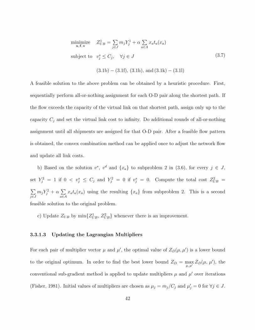
minimizex, f ,v
Z1UB =
∑j∈J
mjY1j + α
∑a∈A
xata(xa)
subject to vsj ≤ Cj, ∀j ∈ J
(3.1b)− (3.1f), (3.1h), and (3.1k)− (3.1l)
(3.7)
A feasible solution to the above problem can be obtained by a heuristic procedure. First,
sequentially perform all-or-nothing assignment for each O-D pair along the shortest path. If
the flow exceeds the capacity of the virtual link on that shortest path, assign only up to the
capacity Cj and set the virtual link cost to infinity. Do additional rounds of all-or-nothing
assignment until all shipments are assigned for that O-D pair. After a feasible flow pattern
is obtained, the convex combination method can be applied once to adjust the network flow
and update all link costs.
b) Based on the solution vs, vd and xa to subproblem 2 in (3.6), for every j ∈ J ,
set Y 2j = 1 if 0 < vsj ≤ Cj and Y 2
j = 0 if vsj = 0. Compute the total cost Z2UB =∑
j∈JmjY
2j + α
∑a∈A
xata(xa) using the resulting xa from subproblem 2. This is a second
feasible solution to the original problem.
c) Update ZUB by minZ1UB, Z
2UB whenever there is an improvement.
3.3.1.3 Updating the Lagrangian Multipliers
For each pair of multiplier vector µ and µ′, the optimal value of ZD(µ, µ′) is a lower bound
to the original optimum. In order to find the best lower bound ZD = maxµ, µ′
ZD(µ, µ′), the
conventional sub-gradient method is applied to update multipliers µ and µ′ over iterations
(Fisher, 1981). Initial values of multipliers are chosen as µj = mj/Cj and µ′j = 0 for ∀j ∈ J .
42

Then in iteration n, the multiplier is updated for ∀j ∈ J such that:
µj,n+1 = max
0, µj,n − φn(CjYj,n − vsj,n
), (3.8)
µ′j,n+1 = µ′j,n + φn(θvsj,n − vdj,n
). (3.9)
The step size φn+1 is updated such that:
φn+1 =λn [ZUB − ZD(µn, µ
′n)]∑
j∈J
[(CjYj,n − vsj,n
)2+(θvsj,n − vdj,n
)2] , (3.10)
where λn is a control parameter. λn =2 is used for an initial value and it is decreased
by a small amount if ZD(µ, µ′) does not improve after a specified number of iterations.
The iteration terminates when certain criteria are satisfied (e.g., the maximum number of
iterations is reached or ZUB − ZD(µn, µ′n) becomes smaller than a certain tolerance). The
LR algorithm may not always find the exact optimal solution to the original problem; i.e.,
a residual gap may exist between the lower and upper bounds (due to the fact that the
constraints vsj −CjYj ≤ 0 may not be tight even at optimum). In other words, if the optimal
solutions of vsj are not all close to the built refinery capacities, there would be a duality gap.
In such cases, we propose two branch-and-bound (B&B) frameworks to further improve the
solution toward optimality.
43

3.3.2 Branch and Bound
If the duality gap is still non-negligible even after a large number of LR iterations, B&B
can be used to further reduce the gap. We first introduce the traditional B&B approach with
LP relaxation bounding. Then we present an alternative B&B approach with LR bounding.
3.3.2.1 Branch and Bound with LP Relaxation Bounding
We propose to branch on decision variables Yj in conjunction with LP relaxation bounding.
Given the objective function (3.1b), if the integrality constraints (3.1j) are relaxed for some
j ∈ J ′, then constraints (3.1g) will be equivalent to vsj = CjYj for j ∈ J ′. Hence, the optimal
solution to this relaxed problem always satisfies
Yj = vsj/Cj, ∀j ∈ J ′. (3.11)
minimizeY,x, f ,v
∑j∈J\J ′
mjYj + α∑a∈A
xata (xa) +∑j∈J ′
(mj/Cj) vsj
subject to Yj ∈ 0, 1, ∀j ∈ J\J ′
(3.1b)− (3.1f), (3.1h), (3.1i), (3.1k)− (3.1l), and (3.11)
(3.12)
This LP relaxation reduces back to a traffic assignment problem with side constraints in
the B&B context, if (i) variables Yjj∈J\J ′ are the branched variables and hence∑
j∈J\J ′mjYj
can be regarded as a constant term, and (ii) value mj/Cj is regarded as a constant travel
cost for virtual link flow vsj . This problem again can be solved by the convex combination
algorithm. The B&B algorithm uses a depth-first search procedure to determine the next
44

variable to branch on. The major steps are as follows:
a) Initialize J ′ = J . Relax all integrality constraints (3.1j) in the original MINLP (3.1a)-
(3.1l).
b) Select the branching variables by a greedy method. We compute the marginal cost of
adding one candidate location from set J ′ to J\J ′. Then the decision variable with the
smallest marginal cost is branched next.
c) Solve the LP relaxation (3.12) above as a capacitated traffic assignment problem with
side constraints. Here we used the modified Frank-Wolfe algorithm presented by Daganzo
(1977a, b). A heuristic technique is devised when assign outbound flow from refineries to
ensure constraints (3.1i) are satisfied.
d) At the beginning of the B&B algorithm, the upper bound from the LR algorithm in
section 7.2.2.1 is adopted as an initial upper bound. Whenever the objective value of the LP
subproblem at the current branching node is larger than the upper bound, further branching
from this node is not necessary. There are three criteria to trim the depth first search tree:
(i) if the subproblem at the current node does not yield any solution (i.e., infeasible),
(ii) if the objective value of the current node is larger than the current upper bound,
(iii) if the optimal solution at the current node is feasible to the original MINLP.
The efficiency of the B&B algorithm (e.g., the percentage of trimmed branches) highly
depends on the quality of the lower bound provided at each branching node (Fisher, 1981).
If the algorithm takes too much time to finish the search, some tolerance may be applied to
the lower bound to trim more branches in B&B algorithms.
45

3.3.2.2 Branch and Bound with LR Bounding
It is well-known that LR provides a tighter lower bound than LP relaxation (Fisher, 1981).
Hence, although our LP relaxation problem is much easier to solve, it is worthwhile to
incorporate an LR bounding procedure into a similar B&B framework. Here, the LR based
lower bound procedure is applied to solve an LR subproblem at each branching node, where
the decision variables Yj’s for ∀j ∈ J\J ′ have been branched on. We use piecewise functions
to represent the travel time of virtual links; i.e., for ∀j ∈ J\J ′, tj(vsj ) = 0 if Yj=1 and
tj(vsj ) → ∞ if Yj=0 . Thus the LR subproblem at a branching node can be rewritten as
follows:
minimizeY,x, f ,v
∑j∈J\J ′
mjYj +∑
j∈J\J ′vsj[tj(v
sj ) + θµ′j
]+ α
∑a∈A
xata(xa) +∑j∈J ′
(mj − µjCj)Yj
+∑j∈J ′
(µj + θµ′j
)vsj +
∑j∈J
(−µ′j
)vdj
subject to Yj ∈ 0, 1, ∀j ∈ J\J ′
(3.1b)− (3.1f), (3.1h), (3.1i), and (3.1k)− (3.1l),
(3.13)
In the branch-and-bound algorithm, if a parent node is not trimmed, the sub-gradient
optimization discussed in section 7.2.2.1 is applied to the corresponding subproblems at the
two child nodes. The variable Yj, ∀j ∈ J ′, with the biggest violation to the relaxed constraints
vsj ≤ CjYj will be branched next. The multiplier µj and µ′j for the LR subproblems at child
nodes are initialized with the best multipliers obtained at the parent node (Mazzola, 1998).
46

3.4 Numerical Tests
A set of numerical experiments are performed to test the computational performance of
the suggested solution algorithms. All algorithms are coded in VC++ and run on a desktop
computer with 2.20 GHz CPU and 1.99 GB memory.
The proposed model is applied to three examples, (i) a 12-node network from Daskin
(1995), as shown in Figure 3.2(a), (ii) the Sioux Falls network (Bar-Gera, 2009), as shown in
Figure 3.2(b), and (iii) the Anaheim network (Bar-Gera, 2009), as shown in Figure 3.2(c).
In all three examples, every network node is both a biomass shipment origin and ethanol
shipment destination. A subset of the nodes is chosen as the refinery candidate sites. The
BPR (U.S. Bureau of Public Roads) function is adopted as the link performance function,
ta(xa) = t0a
(1 + 0.15
(xaCa
)β), (3.14)
where β = 4, and t0a and Ca are respectively the free flow travel time and the traffic capacity
of roadway link a (Sheffi, 1985). In all cases α = 1 is used and the maximum iteration
numbers for traffic assignment subproblems in LR heuristics, traffic assignment subroutine
in LR and LP procedures, and LR subproblems in B&B are 100, 50 and 100, respectively.
47

(a) (b)
(c)
Figure 3.2: (a)A 12 Node Network (b)The Sioux Falls Network (c)The Anaheim Network
48

Some of the computational results are shown in Table 3.1. For all test examples, the
solutions found by the LR based heuristic (without B&B) are in fact quite close (i.e., less
than 1%) to the true optimal solutions or best known feasible solutions (found by the B&B
algorithms). However, in all cases the LR based heuristic method leaves a small residual gap
between the upper and lower bounds. In the 12 nodes and the Sioux Falls cases, B&B with
LP and B&B with LR successfully closed the residual gap and found the optimal solution. In
the Anaheim network example, due to the relatively larger scale, LR based heuristic method
is able to provide a good feasible solution within a reasonable amount of computation time.
The B&B with LP or LR takes a very long time but improves the solution.
Table 3.1: Computational Results of the Test Problems
In general, the LR based heuristic method produces acceptable near-optimum solutions
within a relatively short computation time, but it may leave a small residual gap between the
upper and lower bounds. In such cases, the B&B algorithms with either LP or LR bounding
procedure are able to close (or reduce) the gap. We do note that for large scale problems,
we may not always be able to guarantee the exact optimal solution.
49

3.5 Illinois Case Study
Illinois is currently one of the leading states for U.S. bio-ethanol production, and it is
expected to produce a large share of the national ethanol mandate for years 2007-2022 (Kang
et al., 2008). Therefore we conduct an empirical case study for the State of Illinois in 2022.
The purpose is not only to illustrate the proposed methodology in a realistic context, but
also to cast insights into the impacts of biofuel industry expansion on the transportation
system.
3.5.1 Assumptions and Data Preparation
Figure 3.3.2.2 illustrates the Illinois transportation network, which has 98 nodes (the
centroids of counties 7 and major junctions in the interstate highway network) and 374 links
(interstate highway and local highway). Each node represents both an origin of biomass
supply and a destination of ethanol consumption.
According to the 2007 EPA mandate, the national target for ethanol production is 15
billion gallons from corn and 21 billion gallons from cellulosic biomass and other renewable
biomass in 2022 (U.S. EPA, 2007). We assume that Illinois produces 45% of national ethanol
from all its 102 counties (Syngenta, 2006). The amount of corn and cellulosic biomass
produced in each county in 2022 is calculated based on the share of corn biomass production
in year 2008 (Khanna et al., 2008; Kang et al., 2008). The biomass and ethanol truck flow
is estimated based on full-truck load in volume and then unified to an equivalent number
of passenger cars per hour. The general criteria for selecting biorefinery locations include
7A few county centers close to the intersections of interstate highway are aggregated as one node.
50

access to major transportation facilities, water availability and proximity to biomass supply
regions (Peluso et al., 1998; SEARCY, 2007). In Illinois, water is sufficiently available from
major surface water sources and underground aquifers in most counties (Tursun et al., 2008).
Therefore, we selected 20 candidate biorefinery locations including major interstate highway
junctions and centroids of those counties with large biomass supply.
The refinery capacity is assumed to be 300 million gallons per year and the annual
prorated cost for building such a refinery is $27,000,000 (Kang et al., 2008). The construction
cost is originally obtained from the “Dry Mill Simulator” component of Farm Analysis and
Solution Tools (FAST) by Ellinger (2008). The refinery construction cost is further prorated
into hourly cost by assuming 20 years of service life and 260 days per year and 9 hours per day
as the effective working time for the biomass and ethanol shipping. The hourly background
traffic flow and the roadway information are obtained from the National Transportation
Atlas Database (RITA, 2008) and the Illinois daily traffic database (IDOT, 2007). As a base
scenario, the potential background traffic volume in 2022 is projected from 2007 data with
a 3% annual growth rate. The BPR link performance function (3.14) is again adopted. The
capacity of interstate highway and local highway is assumed to be 2200 and 1700 passenger
car per hour per lane (pcphpl) respectively (HCM, 2000). The free flow speeds on interstates
and local highway are assumed to be 65 mph and 55 mph respectively. Link travel cost is
estimated by the travel time on each link multiplied with an assumed value of travel time
α=$20/hour-passenger car ($20/hr-pc) 8. A thorough sensitivity analysis with regard to
8Various studies have obtained estimates of time values for different traveler types and travel conditions.Generally, the value of travel time depends on many factors, such as purpose of trip, wage rate, region,year, type of vehicle, etc. The recommended value of hourly travel time per person is around 50%-120% of
51

these parameters is presented in section 3.5.3.
Figure 3.3: Transportation network used for analysis in the State of Illinois
3.5.2 Computational Results and Analysis
To study the impact of traffic congestion on the total system cost, two designs are consid-
ered while the values of parameters α, β and the annual traffic growth rate are assumed to be
20 ($/hr-pc), 4 and 3%, respectively. The first design (ignoring the congestion effect) is ob-
tained from a regular fixed charge facility location problem in which all biomass and ethanol
shipment traffic in 2022 are simply assigned along shortest-distance paths. The second de-
hourly wage rate (Litman, 2009), and the median hourly wage rate in Illinois ranges from $11 to $26 by jobtypes (PayScale, 2010). Considering that the average occupancy for passenger cars is 1.59 passengers per car(U.S.DOT, 2009), a rough range of the average value of travel time per hour per passenger car is between$8 and $42.
52

sign is obtained from the proposed model (3.1a)-(3.1l) which considers travel congestion and
optimizes shipment routing. A fairly good feasible solution is found in the second design by
LR heuristic algorithm within about 490 seconds but leaving a small 0.76% gap. The B&B
algorithm with LR bounding reduces the residual gap to 0.3% after solving 149 B&B nodes
in 14933 seconds 9.
For comparison, we compute the itemized costs of both designs under the same maximum
0.3% gap tolerance in Table 3.2. However, the congestion experienced by the shipment fleet
and the public (i.e., background flow) are quite different. For example, compared to the
benchmark, the design with congestion consideration saves biomass shipment cost by more
than 59.84%, while the public total travel cost is reduced by 0.50%. Meanwhile, the impact
of biofuel traffic to the general public is smaller when congestion is considered in the design.
For example, the net increase of the total public travel cost (background flow cost) is only
by 0.16% after loading the biomass and ethanol shipment flow, whereas the number is 0.67%
for the benchmark design. We also note that the benchmark design tends to build fewer
refineries to save fixed cost, leading to much higher transportation cost for both the biofuel
industry and the general public.
9It is possible to further reduce the gap to 0.1% after solving 931 B&B nodes in about 92800 seconds.
53

Table 3.2: Comparison of Two Designs in the Illinois Case Study
We have shown that transportation cost can be reduced for the biofuel company at the
optimal solution compared to the benchmark model. This provides an incentive for the
biofuel company to take these optimal routes considering the congestion effect. Besides,
toll can also be added in the network to influence drivers’ route choice towards the optimal
routings for shipping biomass and biofuel. However, it is not immediately obvious to see on
how tolls on different roads should be set to induce drivers to take right routes that achieve
the social optimum. It is worthy of investigation in another research topic to find out the
optimal toll levels in a road network to minimize the congestion.
3.5.3 Sensitivity to Parameters
The optimal system design and congestion impact depend, to some extent, on the value
of several important parameters, such as the time value α, annual traffic growth rate and the
BPR parameter β. The base-case parameters are the same as those in the previous section;
i.e., α = 20, β = 4 and the annual traffic growth rate is 3%. In the sensitivity analysis,
only one parameter varies at a time, while other parameters remain unchanged. We hence
conduct a series of sensitivity analyses to examine the impact of these parameters. All cases
54

are solved with B&B with LR to a 0.3% optimality gap.
Figure 3.3.2.2 shows how the value of α influences the optimal number of refineries and
roadway congestion impact (i.e., percentage increase of the total transportation cost due
to biomass/ethanol shipments), when all other parameter values are the same as those in
the base scenario. When α increases within the range [10, 60] (implying a larger weight on
transportation cost), more refineries are built to save transportation cost. When α drops
below 10, the optimal number of refineries stays at about six in order to meet the total
production requirement. When α exceeds 60 (a very high value), all 20 candidate locations
have been chosen to build refineries. It can also be seen that when α increases from 0 to
10, the congestion impact decreases slightly. However, as more refineries are built to save
transportation cost (when α > 20), the congestion level becomes generally insensitive to the
value of α .
Figure 3.4: Impact of time value α on the optimal number of refineries and the resulting
congestion
55

Figure 3.3.2.2 illustrates the sensitivity of the optimal number of refineries and congestion
impact to the annual background traffic growth rate. Under higher annual traffic growth rate,
the optimal number of refineries is larger. This is intuitive because when the background
traffic approaches capacity, the model would choose to build more refineries to reduce high
transportation cost. We also observe that the congestion level generally declines when back-
ground traffic growth rate increases, probably because more refineries are built so that the
biomass and ethanol shipment demand (and congestion impact) decreases. Obviously, the
refinery infrastructure design affects, and is affected by, the roadway congestion pattern.
Figure 3.5: Impact of annual traffic growth rate on the optimal number of refineries and the
resulting congestion
Figure 3.3.2.2 illustrates the sensitivity of the optimal number of refineries and congestion
impact to the BPR function parameter β. It seems that the number of refineries is insensitive
to the value of β. When β < 1, the link costs are insensitive to the biomass/ethanol traffic,
56

and hence the congestion impacts are low. As β increases, the link costs become more
sensitive to the biomass/ethanol flow added to the network, and the congestion impact
becomes more evident. When β > 3, the cost component (xa/Ca)β in the BPR function is
reduced sharply since most links have xa/Ca < 1, thus resulting in diminishing congestion
impact.
Figure 3.6: Impact of parameter β on the optimal number of refineries and the resulting
congestion
In our experiments, we also find that the computation time of the B&B algorithms tends
to decrease gradually (for the same gap tolerance) when any of the parameters (i.e., α, β, or
the annual traffic growth rate) increases. This is probably because larger parameter values
imply higher weight of transportation cost or larger impact of biofuel related shipment on
existing traffic. As such, the optimal solution tends to include more refineries, which leads to
more branch cuts in the early stages of the B&B algorithm. For extremely large parameter
57

values, all 20 locations will be chosen, and the B&B algorithm would directly search down
to the optimal branch because all other branches bear much higher objective values.
58

Chapter 4
Joint Optimization of Biofuel SupplyChain Design and Highway PavementRehabilitation Plan Under TrafficEquilibrium
As discussed in Chapter 3, expansion of the biofuel industries leads to construction of
new refineries, which induce additional traffic demand in the highway network for shipping
massive amount of biomass and ethanol to or from these refinery locations. This imposes
pressure on the existing highway transportation infrastructure especially due to the heavy
trucks, which has a major impact on not only the traffic congestion but also highway pave-
ment deterioration. Hence, it is important to design a biofuel supply chain in a holistic
manner, simultaneously taking into account the routing of the trucks as well as the impact
on pavement rehabilitation planning.
This chapter presents an integrated modeling framework for a biofuel supply chain de-
sign which incorporates traffic routing under congestion and pavement rehabilitation under
deterioration, which is an extension of chapter 3. Our model minimizes the total refinery
investment, transportation delay, along with life cycle costs of the pavement refineries. This
59

model is an extension of the MINLP problem (3.1), but a different type of mathematical
program, i.e., a bi-level MINLP, which is developed to simultaneously determine the optimal
number and location of refineries, optimal routing of biomass and ethanol shipments, and
optimal pavement rehabilitation frequency and intensity under traffic equilibrium of existing
road users. A reformulation and LR solution framework is developed to solve the problem
and get optimal solutions. A numerical case study on a hypothetical transportation network
is conducted, and the computational results show that the proposed algorithm is able to
solve the problem effectively.
The model formulation and solution methodology are sufficiently generic to address
general network design problems under user equilibrium for the expansion of any traffic-
attraction refineries (e.g., stadium and shopping malls).
4.1 Model Formulation
This section proposes a bi-level mixed integer non-linear program to simultaneously address
refinery location, materials/products shipment and background traffic routing under con-
gestion, and pavement rehabilitation. The objective is to (i) model the impact of biofuel
supply chain expansion on the supporting transportation infrastructures; and (ii) minimize
the total costs related to the biofuel supply chain (refinery construction, materials/products
transportation cost, public travel delay) and the pavement infrastructures.
4.1.1 Pavement Rehabilitation and Life-cycle Cost
In this section, we first present the pavement deterioration and rehabilitation models that
60

we adopt to derive the user and agency cost functions. We focus on a network pavement
rehabilitation problem, in which the highway network in the study area is represented by a
set of highway links A and a set of nodes V . We consider an infinite time horizon, in which
the cost for the agency during each rehabilitation interval can be prorated into average
cost per unit time. Each single road segment in the network needs an individual pavement
rehabilitation plan. We follow the notations in Ouyang and Madanat (2006) and adopt their
analytical results for a single pavement’s rehabilitation optimization model. All variables
in the pavement model should be associated with a link a ∈ A; for the ease of notation,
however, we will omit subscript a in this section, and will add it later.
Let τ1, τ2, ... denote the discrete time points for rehabilitation activities on each link. Our
decision variables include the time interval between two consecutive rehabilitation activities,
∆τ , and the rehabilitation intensity (i.e., thickness of the overlay), w, on each road segment.
The agency costs for pavement rehabilitation include a fixed initial cost of labor, operation,
etc., and a variable cost dependent upon rehabilitation intensity. According to Ouyang and
Madanat (2006), the agency cost M(w) for a rehabilitation activity of intensity w on one
link with the length l can be modeled as a linear function:
M(w) = l ∗m1 ∗ w, (4.1)
where m1 ≥ 0 is a cost parameter for paving each unit thickness of rehabilitation materials
per unit length of pavement and l is the length of pavement. In practice, m1 usually includes
the set-up cost for constructing pavement, so the total agency cost can be calculated in
61

proportion to the thickness. Assuming a constant bulk specific gravity (i.e., 92%-95%)
and width of the pavement (i.e., 44 feet for two lance highway), we can calculate m1 for
constructing per mile of pavement segment for each inch of overlay based on the material
cost (per ton).
We denote s(τ) as a continuous pavement condition indicator (i.e., roughness) at time
τ ∈ (τi, τi+1), and according to Paterson (1990), the effectiveness in reducing roughness can
be represented as a function of intensity and the road condition before resurfacing (Ouyang
and Madanat, 2006):
∆s(b) = s(τ−i )− s(τ+i ) = G(w, s(τ−i )) =
g1w
g2 + g3/s(τ−i ), (4.2)
and,
w ≤ g2s(τ−i ) + g3, (4.3)
where s(τ−i ) and s(τ+i ) are the values of the pavement roughness before and after the reha-
bilitation activity, and g1 ≥ 0, g2 ≥ 0, g3 ≥ 0 are constant parameters based on empirical
data in Paterson (1990).
User cost includes the transportation cost for freight traffic in the new biofuel supply
chain and the travel cost for the existing road users. Both parts can be further divided into
vehicle operating cost and delay cost; the former is approximately proportional to pavement
roughness, thus the vehicle operating cost per unit time-length, cr(·), can be modeled as a
62

linear function of s(t) as follows.
cr(s(t)) = c1s(t) + c2, ∀t (4.4)
where c1 ≥ 0 and c2 ≥ 0 depend on the properties of the pavement, and they are assumed
to be fixed over time. However the delay cost, is a function of factors such as traffic volume
and road capacity that are not directly related to pavement roughness. It is assumed that
the travel time t(x, z) on each link can be modeled by the commonly used BPR function
(U.S. Bureau of Public Roads), i.e.,
t(x, z) = t0
1 + α
(x+ z
ψ
)β(4.5)
where x denotes biofuel related freight flow, z represents the background traffic flow which
are the traffic related to the existing OD demand, and ψ denotes the link capacity (Sheffi,
1985). Therefore, the user cost per unit time per passenger car1 can be written as follows.
C(x, z) = c0t(x, z) + l(c1s(t) + c2), (4.6)
where c0 ≥ 0 is the value-of-time coefficient that converts travel time into cost.
1To unify the cost components, both biofuel and background traffic volumes are converted into theequivalent number of pc/hr. The detailed converting factor can be found in Highway Capacity Manual(HCM, 2000).
63

Figure 4.1: Deterioration trajectory for a single pavement segment
Pavement roughness on each road segment increases continuously over time between con-
secutive rehabilitation activities, and this process is often described by an exponential func-
tion as below (Tsunokawa and Schofer, 1994; Li and Madanat, 2002; Ouyang and Madanat,
2004):
s(t) = F (s(τ+), t− τ) = s(τ+)eb(t−τ), ∀τ, (4.7)
where variable b > 0 denotes the pavement deterioration rate, which depends on pavement
facility characteristics and traffic volume.
Note that roughness is not the only pavement performance index, but in this work, we
use roughness for simplicity. Pavement rehabilitation triggering condition (i.e., the failure
criteria) can be dominated by structural or functional (e.g., roughness) distress. Pavement
deterioration is due to fatigue, rutting, environmental cracks and the combined effects.
Ouyang and Madanat (2006) showed that the pavement roughness under the optimal
rehabilitation plan should exhibit a cyclic trajectory that has a saw-tooth shape with a
constant threshold roughness for triggering rehabilitation at s∗ = s(τ−i ) for all τi. As in
64

Figure 4.1, the area under the trajectory represents the user cost, and the vertical jumps
represents the agency cost. The trigger roughness as a function of deterioration rate b is as
follows:
s∗(b) =r(m1g3)
c1g1(x+ z) + (b− r)m1g2
, (4.8)
where parameter r is the annual discount rate. Therefore, the optimal rehabilitation intensity
is also a function of b, as follows,
w∗(b) = g2r(m1g3)
c1g1(x+ z) + (b− r)m1g2
+ g3. (4.9)
The change in roughness after each optimal rehabilitation activity ∆τ is as follows:
∆s(b) = (s∗(b)−∆s(b))eb∆τ , (4.10)
and therefore,
∆τ(b) = log(∆s(b)
s∗(b)−∆s(b))b−1. (4.11)
With these analytical results, we can derive the average user cost and agency cost per
unit of time. The user cost under the optimal rehabilitation plan can be written as a function
of traffic and deterioration rate, as follows
65

C(x, z, b) = c0t(x, z) + l
(c1(x+ z)
r(m1g3)
c1g1(x+ z) + (b− r)m1g2
(2g1 − 1)log−1 g1
1− g1
+ c2
).
(4.12)
Furthermore, the prorated annual agency cost becomes the following.
M(b) =π1(x+ z)b+ π2b
2
π3 + π4b+ π5(x+ z), (4.13)
where π1 = lc1g1(g3m1), π2 = lm21g2g3, π3 = −rm1g2log( g1
1−g1 ), and π4 = m1g2log( g11−g1 ), and
π5 = g1c1log( g11−g1 ).
As is mentioned earlier, this work adopts the simplified pavement performance model in
Ouyang and Madanat (2006) that does not reflect the combined effects of structural and
functional damage. So it is worthwhile to study how to incorporate the more advanced
pavement performance model. One immediate step to improve this research is to develop a
realistic pavement condition deterioration function with traffic based on other more advanced
pavement performance models, such as the MEPDG model in the Mechanistic-Empirical
Pavement Design Guide (MEPDG) (NCHRP, 2004).
4.1.2 Supply Chain Design
This section introduces the notation and formulation of the integrated biofuel supply chain
design model. We let J represent the set of candidate locations to build refineries with a
maximum capacity of hj and a fixed cost of ηj, j ∈ J . The selection of locations for refineries
66

is determined by a set of binary decision variables yj, j ∈ J, where yj = 1 if a refinery is
built at j ∈ J or yj = 0 otherwise. We let I and N represent the sets of biomass supply (i.e.,
farms) and demand locations (i.e., gas stations), respectively, while Qi and Qn represent the
total amount of biomass from farmer i ∈ I and total demand for ethanol by gas station
n ∈ N respectively. Variables qiju and qjnu denote the decision variable of the transportation
demand between farm i ∈ I, candidate location j ∈ J , and gas station n ∈ N . In a given
highway network G(V,A), traffic goes through the set of links A. Let f ija denote the path
flow from farm i ∈ I and gas station n ∈ N on link a ∈ A. Let xa denote the shipment flow
on link a ∈ A. In addition, there is a background traffic flow za on each link a ∈ A.
The mathematical optimization model for the integrated biofuel supply chain design can
67
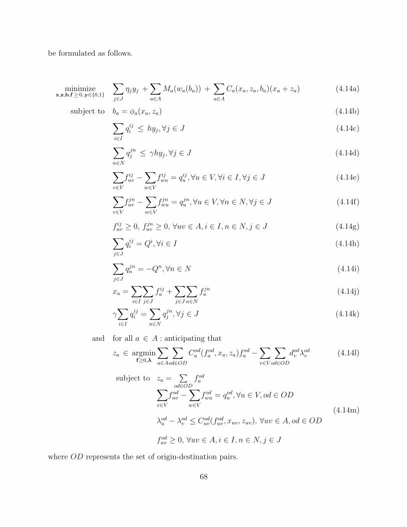
be formulated as follows.
minimizex,z,b,f ≥ 0,y∈0,1
∑j∈J
ηjyj +∑a∈A
Ma(wa(ba)) +∑a∈A
Ca(xa, za, ba)(xa + za) (4.14a)
subject to ba = φa(xa, za) (4.14b)∑i∈I
qiji ≤ hyj,∀j ∈ J (4.14c)
∑n∈N
qjnj ≤ γhyj,∀j ∈ J (4.14d)
∑v∈V
f ijuv −∑w∈V
f ijwu = qiju , ∀u ∈ V, ∀i ∈ I,∀j ∈ J (4.14e)
∑v∈V
f jnuv −∑w∈V
f jnwu = qjnu ,∀u ∈ V, ∀n ∈ N,∀j ∈ J (4.14f)
f ijuv ≥ 0, f jnuv ≥ 0, ∀uv ∈ A, i ∈ I, n ∈ N, j ∈ J (4.14g)∑j∈J
qiji = Qi,∀i ∈ I (4.14h)
∑j∈J
qjnn = −Qn,∀n ∈ N (4.14i)
xa =∑i∈I
∑j∈J
f ija +∑j∈J
∑n∈N
f jna (4.14j)
γ∑i∈I
qiji =∑n∈N
qjnj ,∀j ∈ J (4.14k)
and for all a ∈ A : anticipating that
za ∈ argminf≥0,λ
∑a∈A
∑od∈OD
Coda (f oda , xa, za)f
oda −
∑v∈V
∑od∈OD
dodv λodv (4.14l)
subject to za =∑
od∈ODf oda∑
v∈V
f oduv −∑w∈V
f odwu = qodu ,∀u ∈ V, od ∈ OD
λodu − λodv ≤ Coduv(f
oduv , xuv, zuv), ∀uv ∈ A, od ∈ OD
f oduv ≥ 0, ∀uv ∈ A, i ∈ I, n ∈ N, j ∈ J
(4.14m)
where OD represents the set of origin-destination pairs.
68

The objective function (4.14a) minimizes the total system cost which includes refinery
construction investment, pavement agency cost, and user cost, respectively. Constraints
(4.14b) define the pavement deterioration rate on each link a ∈ A as a function of total
traffic. Constraints (4.14c) (and (4.14d)) ensure that the supply (and demand) throughput
at each candidate refinery location cannot be greater than its maximum production capacity.
Constraints (4.14e) indicate the transportation demand for biomass in farm i ∈ I and ethanol
for gas station n ∈ N . Constraints (4.14g) define the non-negativity constraints. Constraints
(4.14h) and (4.14i) stipulate that the sum of all biomass flows out of all farms should be
equal to the total supply at that refinery, and all ethanol shipment flows into a gas station
should be equal to the total demand at that point. Constraints (4.14j) defines the link flow
for freight traffic on each link. Constraints (4.14k) ensure flow conservation at the refinery
j ∈ J , indicating that the inbound biomass flow converts to the equivalent ethanol outbound
flow at each refinery; parameter γ is the volume-based convertor from biomass to ethanol.
Finally, the lower level problem (4.14l) with constraints (4.14m) define the background (i.e.,
public) traffic flow za on each link a ∈ A.
4.2 Solution Technique
We apply the Lagrangian relaxation (LR) approach to separate the discrete location variables
(sub-problem 1) from all other continuous variables (sub-problem 2) (Bai et al., 2011b). We
first relax constraints (4.14c) and (4.14d) and add them as penalty terms to the objective
with Lagrangian dual variables µ1 = µ1j ≥ 0 and µ2 = µ2
j ≥ 0. This procedure leads to
69

the following relaxed problem:
L(µ1,µ2) = minimizey∈0,1 x,z,b,≥ 0
∑j∈J
ηjyj +∑a∈A
Ma(wa(ba)) +∑a∈A
Ca(xa, za, ba)(xa + za)
+∑j∈J
µ1j(∑i∈I
qiji − hyj) +∑j∈J
µ2j(∑n∈N
qjnj − γhyj) (4.15)
subject to (4.14b) and (4.14e)− (4.14m).
With no other constraints on y, the above relaxed problem can be decomposed into two
sub-problems. One sub-problem contains only binary variables.
(Sub-problem 1)
minimizey
∑j∈J
(ηj − h(µ1j + γµ2
j))yj
subject to yj ∈ 0, 1 , ∀ j ∈ J
(4.16)
and the other sub-problem is a continuous bi-level nonlinear program (NLP).
(Sub-problem 2)
minimizex,z,b≥ 0
∑a∈A
Ma(wa(ba)) +∑a∈A
Ca(xa, za, ba)(xa + za) +∑j∈J
µ1j
∑i∈I
qiji
+γ∑j∈J
µ2j
∑n∈N
qjnj (4.17)
subject to (4.14b), (4.14e)− (4.14m), (4.14k), and∑i∈I
qiji ≤ h (4.18)∑n∈N
qjnj ≤ γh. (4.19)
Note that we added two additional constraints (4.18) and (4.19) (redundant to the original
70

problem) to facilitate the solution speed for sub-problem 2.
For any given µ, sub-problem 1 can be solved by simple inspection. Sub-problem 2
contains only continuous variables, but it is still difficult to solve. We will present a complete
algorithm to solve sub-problem 2 in Section 4.2.1. As such, the relaxed problem (4.15) can
be solved, and the relaxed objective provides a lower bound to the original problem (4.14).
Standard framework of the LR algorithm can be used to iteratively search for the optimal
value of dual multipliers µ based on a conventional sub-gradient method. In iteration ε, µ
can be updated by:
µ1j,ε+1 = max
0, µ1
j,ε + tε
(∑i∈I
qiji − hyj)
)(4.20)
µ2j,ε+1 = max
0, µ2
j,ε + tε
(∑n∈N
qjnj − γhyj)
)(4.21)
where tε denotes the step size in the εth iteration. There are multiple ways to update the
step size; however, one popular choice is as follows:
tε+1 =ξε (UB − LB)∑
j∈J
((∑i∈I
qiji − hyj)2 + (∑n∈N
qjnj − γhyj)2), (4.22)
where ξε is a scalar control parameter that can be gradually reduced over the iterations.
4.2.1 Solving Sub-Problem 2
For any given value of µ, subproblem 2 is still challenging because it is a bi-level NLP. We
adopt the analytical results in (Lu, 2006) so that subproblem 2 can be reformulated into an
71

equivalent single level problem and solved by an iterative procedure.
We introduce a large enough penalty parameter, θ > 0, on the objective function in
(4.14l) and add it in the upper level objective function (4.14a). We also plug function
ba = φ(xa, za) into the model so as to reduce the number of variables. Now, we have a single
level problem as follows.
minimizex,z≥0,q
∑a∈A
Ma(xa, za) +∑a∈A
Ca(xa, za)(xa + za) +∑j∈J
µ1j
∑i∈I
qiji + γ∑j∈J
µ2j
∑n∈N
qjnj
+θ(∑a∈A
∑od∈OD
Coda (f oda , xa)f
oda −
∑v∈V
∑od∈OD
dodv λodv ) (4.23)
subject to (4.14b), (4.14e)− (4.14i) and (4.14m).
where
Ma(xa, za) = lm1
(g2r(m1g3)
c1g1(xa + za) + (φ(xa, za)− r)m1g2
+ g3
), (4.24)
Ca(xa, za) = c0ta(xa, za) + lc1r(m1g3)
c1g1(xa + za) + (φ(xa, za)− r)m1g2
(2g1 − 1)log−1 g1
1− g1
+ lc2
(equation (A.12) Appendix A).
Proposition 1. With a large enough θ, the bi-level problem in (4.17)-(4.19) is equivalent to
the single level optimization problem in (4.23).
Proof. The lower level user equilibrium objective is non-negative (see Lu, 2006, Theorem 3):
∑a∈A
∑od∈OD
Coda (f oda , xa, za)f
oda −
∑v∈V
∑od∈OD
dodv λodv ≥ 0. (4.25)
72

Since arc flow f is said to be in UE if and only if there exists a λ ∈ R|od|×|V | such that the
lower level optimization problem has an optimal value of zero (Lu, 2006). If parameter θ
takes a large enough positive value, the term (4.25) will be forced to become zero, and thus
the UE condition will be satisfied. Therefore, the objective function will be exactly the total
system cost. This completes the proof.
We use an iterative procedure to solve sub-problem 2. First, an initial value for θ is
chosen, and the single level problem (4.23) is solved by an NLP algorithm. If we find an
optimal solution to this problem, we check the value of the lower level problem in (4.14l): if
the objective value is zero we terminate the algorithm, otherwise we increase the value of θ
and again solve the NLP problem using the updated θ. If the optimal solution to (4.23) is
not found, we decrease θ and solve the NLP problem using this updated value.
To make sure that the lower bound we obtained from solving the relaxed problem (4.15)
is valid, we need to solve sub-problem 2 in (4.23) to exact optimality. We know that if
sub-problem 2 is convex, any local optimal solution is also global optimal. Therefore, as
long as we find a local optimal solution to sub-problem 2 in (4.23), the objective value of the
relaxed problem in (4.15) is optimal and thus is a valid lower bound to the original problem
in (4.14).
To simplify our problem, we further assume that the pavement deterioration rate is a
linear function of traffic volume; i.e.,
ba = φ(xa, za) = e0xa + e1za + e2. (4.26)
73

Then the following proposition holds.
Proposition 2. In an optimal solution, if αω2 − λ ∗ γ − 2Ω1Ω2Ω3 ≥ 0, e2 − r > 0, and
g1 > 0.5, then the objective function (4.23) and constraints (4.14m) are convex.
(where α = π1e0 + π2e20, ω = π3 + π4e2, λ = π1e0 + 2π2e0e2, and γ = π4e0 + π5, Ω1 =
lc1r(m1g3)(2g1 − 1)log−1 g11−g1 , Ω2 = (e2 − r)m1g2, Ω3 = c1g1 +m1g2e0.)
Proof. See Appendix A.
With this Proposition, we have derived the sufficient condition for problem (4.23) to be
a convex program over a non-empty feasible region.
4.2.2 Algorithm Framework
The complete algorithm framework to solve problem (4.14) is as follows.
74

Step 1. Initialize µ0.
Step 2. Solve sub-problem 1 in (7.24) by simple inspection.
Step 3. Solve sub-problem 2.
Step 3.1. Initialize θ0.
Step 3.2. Solve (4.23) under θk by an NLP algorithm, such as interior point method.
Step 3.3. If the optimal solution for (4.23) is found, go to Step 3.4.; otherwise, decreaseθk to θk+1 = θk
δ, then go to Step 3.2.
Step 3.4. If∑
a∈A∑
od∈ODCoda (f oda , xa)f
oda −
∑v∈V∑
od∈ODdodv λ
odv = 0, terminate; other-
wise, increase θk to θk+1 = ρθk, then go to Step 3.2.
Step 4. Find feasible solution to the original problem.
Step 4.1. Fix the values of the continuous variables from sub-problem 2 and solve thelocation decision variables; i.e., set (x, z,λ, f ,q) = (x, z,λ, f ,q)sub2, and theny = 1 if (
∑i∈I q
iji )sub2 > 0 and y = 0 if (
∑i∈I q
iji )sub2 = 0.
Step 4.2. Fix the value of location decision variables y to the relaxed problem fromsub-problem 1 under the current µn, and solve the original problem; i.e., sety = ysub1 and solve (x, z,λ, f ,q) using fixed y.
Step 4.3. Find the best feasible solution from Step 4.1. and Step 4.2.
Step 4.4. Update the upper bound if there is any improvement compared to the currentsolution, and go to Step 5.
Step 5. Compute the optimality gap, terminate if gap is less than tolerance, otherwiseupdate the value of µ according to (4.20)-(4.22), then go to Step 2.
4.3 Numerical Results
The proposed solution procedure is coded in GAMS and run on a desktop computer with
2.67 GHz CPU and 2.00 GB memory. We used Knitro solver to solve the NLP problem
(4.23). We apply our solution algorithm to a hypothetical network with 7 nodes and 32
links; see Figure 4.2. There are 10 OD pairs in this example and 3 candidate locations at
75

nodes 3, 4, and 5. The raw material supply points are at nodes 1 and 2, and the demand
points are at nodes 6 and 7.
Figure 4.2: Hypothetical network
We experiment on 10 cases with randomly generated OD demand data and investi-
gate the effect of parameter θ on the solution and the computation time. The pave-
ment related parameters are from Ouyang and Madanat (2006) and Ouyang (2007): m1 =
11, 000 $/mm/mile and g1 = 0.66, g2 = 0.55mm/QI, g3 = 18.3mm, c0 = 1 $/hr/pc and
c1 = 0.00002 $/QI/veh/year, c2 = 0, e1 = 1.136 × 10⁻⁵ hr/pc/year, e2 = 0.107 year−1. The
discount rate is r = 0.07 year−1. These parameter values satisfy the conditions in Proposition
2.
The biofuel supply chain parameters include the maximum capacity of a production
refinery, h = 2000 per year, the fixed cost for construction a refinery of this size, η = 1.286×
105 $/year, and the volume-based convertor from supply flow to demand flow, γ = 1/2. The
average speed on the network links is assumed to be 65mph, and the free flow travel time on
each link equals length over speed. The link capacity is ψ = 4400 pc/hr, and the constants
76

in the BPR function are α = 0.15 and β = 4.
The algorithm efficiently converges to near-optimum solutions for all test problem in-
stances. With the initial value of θ0 = 105 for all 10 cases, the results including the number
(κ) and location of refineries (%), refinery construction cost (Υ), agency cost (σ), delay cost
(ν), vehicle operating cost (ϕ), user cost (κ), optimality gap, and computation time are
shown in Table 4.1, respectively.
Table 4.1: Total costs and computation times for 10 cases with randomly generated trafficdata
Case κ % Υ (×108 $) σ (×109 $) ν (×109 $) ϕ (×108 $) κ (×109 $) gap (%) run time (Sec)
1 2 3,5 9.000 3.558 2.770 1.828 2.953 0.8 42512 2 3,5 9.000 3.560 2.635 1.705 2.805 0.3 42783 2 3,5 9.000 3.558 2.757 1.820 2.939 2.5 31344 2 3,4 9.000 3.559 2.820 1.789 2.999 1.1 42495 2 4,5 9.000 3.557 2.939 1.887 3.128 1.3 232686 2 3,4 9.000 3.556 3.142 1.906 3.333 0.05 8167 2 4,5 9.000 3.554 3.183 2.018 3.385 0.03 10008 2 3,5 9.000 3.559 2.665 1.750 2.840 0.06 3809 2 3,4 9.000 3.558 3.049 1.811 3.230 0.3 949210 2 3,5 9.000 3.555 3.052 1.961 3.248 1.8 4336
We have also conducted a series of sensitivity analyses to draw managerial insights into
the effects of initial θ value on the computation time. The results are shown in (Figure 4.3),
where θ0 ∈ 102, 5× 10², 103, 5× 10³, 5× 10⁴, 105, 5× 10⁵, 106, 15× 105 is used as the initial
value of θ.
77

Figure 4.3: Sensitivity analysis for θ0
Note that in general, the higher value of θ0, the less computation time is needed to reach
the optimality. According to Step 3 of our solution algorithm in Section 4.2.2, if θ is small
and the optimal solution to the UE problem (4.14l)-(4.14m) is not found, we need to increase
θ through more iterations to finally get the optimal solution. This generally requires more
computation time. Furthermore, the number of iterations to find the optimal value of θ is
small if the initial value is large enough, because it guarantees that the objective in the lower
level problem in (4.14a) is zero, i.e.,∑
a∈A∑
od∈ODCoda (f oda , xa)f
oda −
∑v∈V∑
od∈ODdodv λ
odv = 0.
Therefore, we need less computation time to reach the optimality.
To draw some insights from the optimal solution into the optimal design, we compare the
solution of our proposed model with a benchmark solution which is computed by ignoring
the pavement impact. We obtain the benchmark solution from a model similar to the one
we developed in chapter 3. We choose case 1 as an example for the purpose of comparison,
78

and the itemized costs are shown in Table 4.2.
Table 4.2: Comparison of the benchmark solution and the optimal solution
Scenariorefinerylocation
refineryconstructioncost (×109 $)
biomass ðanol trans-portation cost(×109 $)
agencycost(×109 $)
delay cost(×109 $)
vehicleoperat-ing cost(×109 $)
totalusercost(×109 $)
totalsocialcost(×109 $)
benchmark so-lution
3,5 0.90 0.74 12.57 3.25 0.72 3.32 16.34
optimal so-lution to theproposedmodel
3,5 0.90 1.51 5.42 3.67 0.075 3.75 10.00
Comparing the results of the two scenarios, we can see that the proposed model with
joint pavement rehabilitation optimization dramatically reduces the total social cost. In the
benchmark solution, a dominant cost is the agency cost, which is much higher than other
cost components and its counterpart in the optimal solution. This is because if the impact
of pavement deterioration is ignored, there could be certain links with large amount of traffic
forming some kind of “bottlenecks” which would have consequently high deterioration rates.
Since deterioration function is exponential with respect to traffic volume in our model 2, the
agency cost in the benchmark solution becomes significant. While if the impact of traffic on
pavement is considered, the traffic at user equilibrium tends to distribute more evenly in the
network, so that the impact on the whole network pavement condition is modest.
Note that the total user cost in the benchmark solution is smaller than that in the social
optimal solution. This makes sense in that under current parameter values, the delay cost is
the major component, and the benchmark solution actually minimizes the total delay cost
plus the refinery location cost. Therefore without considering the pavement rehabilitation
2This can be seen from equations (4.7) and (4.26).
79

cost, it is likely to provide lower bounds on the user cost. In other words, in the social optimal
design, some of the flow has to be rerouted to save pavement rehabilitation cost, thus may
probably leads to higher user cost. However, given the much lower agency cost, our optimal
solution minimizes the total social cost, which is consistent with our incentives in finding
sustainable biofuel supply chain design solutions with minimal negative social impacts.
For Case 1, the optimal pavement roughness trajectory for road segment 8 is shown in
Figure 4.4, and the deterioration rate b8 = 0.08 year−1, ∆τ(b8) = 9.2 years, and s∗(b8) =
39.8QI, and ∆s(b8) = 20.2QI. The dashed trajectory is from the benchmark solution,
which has a slightly shorter rehabilitation cycle.
Figure 4.4: Optimal roughness trajectories for pavement segment 8 in the hypothetical
network
Our model assumes a centralized system in which all decisions (for both a biofuel company
and the pavement maintenance agency) are made toward the social optimal. Although the
biofuel company in general does not consider the agency cost, its decisions on refinery location
80

and shipment routing affects the long run sustainability of the industry and the society. Our
model shows that the impacts can be significant. So the government may need to add tax
or regulation to the biofuel industry for the damage on pavement. This model gives us
what the best the biofuel industry can do to minimize its impact on the transportation
infrastructure and the social cost, and thus provides the government with some guidelines
on making policies in the future.
81

Chapter 5
Biofuel Supply Chain Design underUncertainties and Risks
In this chapter, we extend our models to account for uncertainties and risks in biofuel
supply chain design. We develop a stochastic version of our supply chain design model that
deals with feedstock supply and ethanol demand uncertainties. From this model, the optimal
supply chain configuration should well balance the trade-off between the expected operational
efficiency under uncertainties and the capital investment cost for building refineries. Monte
Carlo method is adopted to approximate the probabilistic distribution of spatial dependent
supply and demand and expected total system cost by generating a large number of scenarios.
Our methodology is applied to a small test example and a series of numerical results are
discussed.
Besides the feedstock supply and ethanol demand uncertainties, bio-ethanol facilities and
infrastructure are also susceptible to all kinds of disruption hazards, such as water scarcity,
flooding, routine maintenance, or adverse weather condition (Schill, 2008; Stillwater, 2002).
The risks of operation disruptions compromise the efficiency and reliability of the energy
supply system. We applies the discrete and continuous reliable facility location models
82

to the design of reliable bio-ethanol supply chains for the State of Illinois (one of the main
biomass supply states in the U.S.) so that the system can hedge against potential operational
disruptions. The impacts of both site independent and dependent disruptions are analyzed
with a series of numerical experiments.
5.1 Supply and Demand Uncertainties in Biofuel Sup-
ply Chain Network
In most of existing supply chain models, biomass supply and demand is normally assumed
to be exogenous and deterministic. In reality many stochastic factors could actually affect the
design and operation of biofuel supply chain, such as, environmental factors that affect bio-
crop yield, farmland and crop prices, capital investment cost and transportation cost, demand
and market price of bio-ethanol, policy changes, etc. Due to these uncertainties, a supply
chain needs to be designed robust and flexible enough to achieve minimum expected total cost
in the uncertain environment. In this section, we propose a mixed integer nonlinear program
(MINLP) that integrates the conventional fixed-charge facility location model and the traffic
assignment model to simultaneously address biorefinery location and biofuel feedstock and
final product shipment routing decisions under supply and demand uncertainties.
83

Figure 5.1: Methodology framework
The framework of the methodology is shown in Figure 5.1. There are two types of input
data, deterministic data, such as highway capacities and fixed costs for building refineries,
and stochastic data, such as corn supply and ethanol demand. The problem is formulated as
a scenario-based stochastic programming model. Monte Carlo simulation is used to generate
multiple scenarios (i.e., sets of realized random variables) from the stochastic data. The
scenarios and the deterministic data are used as the input to the model. The model is solved
with LR. Feasible solution is obtained by applying Lagrangian heuristic to the solution to the
relaxed problem. In the following subsections, we will first introduce the model formulation
and Lagrangian relaxation algorithm, and then introduce the Monte Carlo simulation method
84

used to generate scenarios.
5.1.1 Model Formulation
Let Is and Id denote respectively the set of corn supply regions (farms) and the set of
ethanol demand regions (gas stations). Farm i ∈ Is produces hsi amount of corn supply that
needs to be shipped to refineries, and region i′ ∈ Id demands hdi′ amount of ethanol, in the
same unit, that needs to be shipped from refineries. Both hsi and hdi′ are random variables
in our problem and follows certain probability distribution with respectively probability
distribution functions gsi (hsi ) and gdi′(h
di′). Correlations exist among random variables hsi ,∀i ∈
Is and among hdi′ , ∀i′ ∈ Id. For example, the corn supply of the farms depends on the yield
of farm lands and will be all affected if some natural disaster happens. Let J be the set of
candidate refinery locations. A refinery at location j ∈ J has a fixed production capacity
of Cj and requires a fixed investment mj, which may vary across locations due to social-
economical factors such as land price. Assume that at most P facilities can be built due to
limited resources. If there is no limitation, we can let P = |J |. We need to determine a
subset of locations for refinery constructions via the following binary decision variables:
Yj =
1, if a facility is built at candidate site j
0, otherwise
Given the selected refinery locations, corn and ethanol need to be shipped to or from
refineries through a transportation network. Let A denote the set of network links. Note
that corn or ethanol can be shipped to or from any refinery as long as its capacity is not
85

exceeded. For convenience, we add to the network an imaginary sink node Ss for corn
shipments, an imaginary source node Sd for ethanol shipments, and a set V of virtual links
that connect candidate location j ∈ J to Ss and Sd, as shown in Figure 5.2. Each farm is
regarded as an origin of a corn shipment trip (with volume hsi ) and node Ss is the (only)
destination. Node Sd is regarded as the origin of all ethanol shipment trips and each ethanol
demand region is a destination. As such, in any feasible solution, all truck flows transporting
corn and originating from the source node go through at least one constructed refinery, and
so do those transporting ethanol and reaching the sink node. The corn and ethanol deliveries
(shipment routes) are endogenously determined in the model.
Figure 5.2: Illustration of entire network representation including the dummy refineries.
On each roadway link a ∈ A, link flow xa consists of background traffic flow ba, corn truck
flow and ethanol truck flow. In this study, for simplicity, we assume that the background
traffic flow is fixed and independent of corn or ethanol shipments. We use f s,ik to denote
corn flow on any possible path k ∈ Ks,i from farm i ∈ Is to the sink node Ss and f i′,dk to
denote ethanol flow on any possible path k ∈ Ki′,d from the source node Sd to gas station
86

i′ ∈ Id, where Ks,i is set of all possible paths from farm i ∈ Is to node Ss, and Ki′,d is the
set of all possible paths from node Sd to gas station i′ ∈ Id. The total link traffic flow can be
expressed as xa = ba+∑i∈Is
∑k∈Ks,i
f s,ik δs,ia,k +∑i∈Id
∑k∈Ki′,d
f i′,dk δi
′,da,k , where δs,ia, k = 1 if link a is a part
of path k ∈ Ks,i connecting O-D pair i−Ss, or δs,ia,k = 0 otherwise; and similarly for δi′,da,k . The
travel time on link a ∈ A, ta(xa), is a function of the total link flow xa. Correspondingly, we
use vsj and vdj to denote the link flow on the virtual links in V , such that
vsj =∑i∈Is
∑k∈Ks,i
f s,ik ∆s,ij,k,
vdj =∑i′∈Id
∑k∈Ki′,d
f i′,dk ∆i′,d
j,k ,
where ∆s,ij,k = 1 if node j is on pathk ∈ Ks,i, or ∆s,i
j,k = 0 otherwise; and similarly for ∆i′,dj,k .
Note that vsj and vdj also represent the refinery throughput at location j.
It is possible that only a part of the corn supply is utilized and transported to refineries,
or only a part of the ethanol demand is met. This happens when supply and demand are not
balanced, or supply/demand is so high that it is not economical to utilize/satisfy all of it.
Therefore, a link is added from every farm to the sink node to discharge the possible surplus
corn flow, and a link is also added from the source node to every gas station to satisfy the
extra demand. The flow from source Ss to gas station i′ ∈ Id is represented by variable f i′,d
0
and that from farm i ∈ Is to sink Sd is represented by variable f s,i0 . These flows neither incur
any costs nor generate any benefits. Let y = Yj, x = xa ∪ vdj and h = hsi ∪ hdi′.
Let B denote the benefit generated by a unit of ethanol transported to gas station. Let θ be
87

the conversion rate of corn and ethanol, i.e., one unit of corn can produce θ units of ethanol.
The problem is formulated as follows:
(M1):
miny
Eh
[minx
(∑j∈J
(mjYj −Bvdj ) + α∑a∈A
(xa − ba)ta(xa)
)]
= miny
(∑j∈J
mjYj + Eh
[minx
(α∑a∈A
(xa − ba)ta(xa)−B∑j∈J
vdj
)])(5.1)
subject to xa = ba +∑i∈Is
∑k∈Ks,i
f s,ik δs,ia,k +∑i∈Id
∑k∈Ki′,d
f i′,dk δi
′,da,k , ∀a ∈ A (5.2)
vsj =∑i∈Is
∑k∈Ks,i
f s,ik ∆s,ij,k, ∀j ∈ J (5.3)
vdj =∑i∈Id
∑k∈Ki′,d
f i′,dk ∆i′,d
j,k , ∀j ∈ J (5.4)
∑k∈Ks,i
f s,ik + f s,i0 = hsi , ∀i ∈ Is (5.5)
∑k∈Ki′,d
f i′,dk + f i
′,d0 = hdi′ , ∀i′ ∈ Id (5.6)
vsj ≤ CjYj, ∀j ∈ J (5.7)
θvsj = vdj , ∀j ∈ J, l ∈ L (5.8)∑j∈J
Yj ≤ P (5.9)
Yj = 0, 1 , ∀j ∈ J (5.10)
f s,ik ≥ 0, ∀i ∈ Is, k ∈ Ks,i ∪ 0 (5.11)
f i′,dk ≥ 0, ∀i′ ∈ Id, k ∈ Ki′,d ∪ 0 (5.12)
88

Objective function (5.1) minimizes expected system costs, including the costs of building
refineries and transporting corn and ethanol, minus the benefits from ethanol transported
to gas stations. Parameter α converts travel time to travel cost, and it also captures the
relative weight of total travel cost against the cost for building refineries and the benefit from
ethanol. Constraints (5.2) state that the traffic flow on link a is the sum of the background
traffic and the equivalent passenger car flow rate for shipping corn and ethanol. Constraints
(5.3) and (5.4) ensure that the flow on each virtual link (j, Ss) and (j, Sd) is the sum of the
corn or ethanol flows on all paths that pass through node j. Constraints (5.5) and 5.6
ensure that the sum of all corn flows out of a corn supply region is equal to the supply at
that region, and that the total ethanol shipment flow into a demand region is equal to the
demand at that region. Constraints 5.7 impose that the refinery throughput vsj at candidate
site j can be any nonnegative value up to the refinery capacity (in traffic volume of corn
unit) if there is a facility at candidate location j (i.e., Yj = 1 ), or vsj should be zero otherwise.
Constraints (5.8) enforce flow conservation at the refineries; i.e., the inbound corn flow can
be converted into an equivalent amount of outbound ethanol flow. Constraint (5.9) is the
budget constraint to ensure no more than P refineries are built. Constraints (5.10) - (5.12)
define the binary and nonnegative variables.
89

5.1.2 Solution Algorithms
5.1.2.1 Scenario Generation
In this study, we assume that the average supply per farm, hs = 1|Is|∑i∈Is
hsi , and the average
demand per gas station, hd = 1
|Id|∑i′∈Id
hdi′ , follow some probability distributions and are
independent. They are affected by global uncertainty factors such as natural disasters. We
also assume that hsi and hdi′ follow some probability distributions. They are affected by both
global uncertainty factors and local uncertainty factors. Therefore, they can be written as:
hsi = hs + ∆hsi , ∀i ∈ Is,
hdi′ = hd + ∆hdi′ , ∀i′ ∈ Id,
where ∆hsi and ∆hdi′ are all independent random variables and only represent local uncer-
tainty factors. For simplicity, we omit the superscripts s and d for hsi and hdi′ , and use hi
to represent both of them. We also do so for Is and Id. There are two stages to generate
random variates hi : first h is generated, and then ∆hi for each i ∈ I. Two variance reduc-
tion techniques, antithetic sampling and stratified sampling (Glasserman, 2004), are applied
when generating random variates. Stratified sampling is applied in the first stage. The real
line is partitioned into k intervals of equal probability under the probability distribution of
h. Because there are two variates to generate: hs and hd, and each of them are generated
in k intervals, there are totally k2 strata. We generate the same number of variates in each
90

stratum. Antithetic sampling is applied in the second stage. For each pair of hs and hd
generated in stage 1, ∆hs1, . . . ,∆hs|Is|, ∆hd1, . . . ,∆h
d
|Id| are generated and are used as one
scenario. Then their antithetic variates ∆hs1, . . . ,∆hs|Is|, ∆hd1, . . . ,∆h
d
|Id| are used as a sec-
ond scenario. Therefore, for each pair of hs and hd, two scenarios are obtained. Intuitively,
antithetic sampling can help improve the solution quality. The refineries tend to be located
close to the farms/gas stations with high supply/demand, so negative dependence in the in-
puts produce negative correlation between the outputs, which is the condition for antithetic
sampling to reduce the variance.
5.1.2.2 Decompose scenarios - Lagrangian Relaxation
M1 can be written as miny∈Y
Eh
[min
x∈Xy,h
z(y,x)
], where Xy,h is the solution space of x, and Y
is that of y. Xy,h is dependent on both y and h. This is a two-stage stochastic program
(Ahmed, 2004), where y are the first stage variables optimized outside of the expectation
sign, and x are the second stage variables optimized within the expectation sign. Because
the random variables in h are continuous and may have a very large number, and Xy,h
is the solution space of a mixed integer program, such stochastic programs are generally
very difficult to solve, even without the first stage variables y. One way to solve such
problems is to use scenario-wise decomposition. Instead of solving the exact model M1,
l = 1, . . . , |L| scenarios, each with a set of random variates hl, are generated, and model
miny∈Y
1|L|
|L|∑l=1
minxl∈Xy,hl
z(y,xl) is used to approximate M1, where xl is the second-stage variables
in scenario l. The model is then formulated as follows:
91

(M2)
miny
∑j∈J
mjYj +1
|L|
|L|∑l=1
minxl
(α∑a∈A
(xa,l − ba)ta(xa,l)−B∑j∈J
vdj,l
) (5.13)
subject to xa,l = ba +∑i∈Is
∑k∈Ks,i
f s,ik,lδs,ia,k +
∑i∈Id
∑k∈Ki′,d
f i′,dk,l δ
i′,da,k , ∀a ∈ A, l ∈ L (5.14)
vsj,l =∑i∈Is
∑k∈Ks,i
f s,ik,l∆s,ij,k, ∀j ∈ J, l ∈ L (5.15)
vdj,l =∑i∈Id
∑k∈Ki′,d
f i′,dk,l ∆i′,d
j,k , ∀j ∈ J, l ∈ L (5.16)
∑k∈Ks,i
f s,ik,l + f s,i0,l = hsi,l, ∀i ∈ Is, l ∈ L (5.17)
∑k∈Ki′,d
f i′,dk,l + f i
′,d0,l = hdi′,l, ∀i′ ∈ Id, l ∈ L (5.18)
vsj,l ≤ CjYj, ∀j ∈ J, l ∈ L (5.19)
θvsj,l = vdj,l, ∀j ∈ J, l ∈ L (5.20)∑j∈J
Yj ≤ P (5.21)
Yj = 0, 1 , ∀j ∈ J (5.22)
f s,ik,l ≥ 0, ∀i ∈ Is, k ∈ Ks,i ∪ 0, l ∈ L (5.23)
f i′,dk,l ≥ 0, ∀i′ ∈ Id, k ∈ Ki′,d ∪ 0, l ∈ L (5.24)
The first stage variables Yj can be split into multiple instances Yj,l for each scenario l.
Then the model becomes:
92

(M3)
miny,x
1
|L|
|L|∑l=1
(∑j∈J
mjYj,l + α∑a∈A
(xa,l − ba)ta(xa,l)−B∑j∈J
vdj,l
)(5.25)
subject to (5.14) − (5.18), (5.20), (5.22), (5.24)
Yj,1 = Yj,2 = . . . = Yj,l, ∀j ∈ J (5.26)
vsj,l ≤ CjYj,l, ∀j ∈ J, l ∈ L (5.27)∑j∈J
Yj,l ≤ P, ∀l ∈ L (5.28)
Yj,l = 0, 1 , ∀j ∈ J, l ∈ L (5.29)
where (5.26) are called “non-anticipativity” constraints. They are the only constraints which
interrelate the variables across different scenarios. We solve this model using LR (Fisher,
1981). (5.26) is relaxed and the problem is decomposed into subproblems, one for each
scenario. The objective of the relaxed problem is:
(M4)
miny,x
1
|L|
|L|∑l=1
(∑j∈J
(mjYj,l −Bvdj,l) + α∑a∈A
(xa,l − ba)ta(xa,l)
)+
|L|∑l=2
∑j∈J
ξj,l(Yj,l − Yj,1)
(5.30)
where ξj,l, l = 2, . . . , |L| are LR multipliers for constraints (3.b). Define ξj,1 = −|L|∑l=2
ξj,l. The
objective of each subproblem l ∈ L becomes:
93
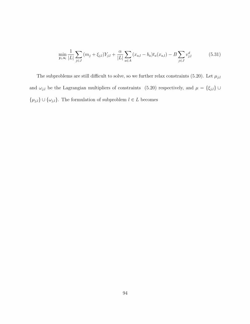
minyl,xl
1
|L|∑j∈J
(mj + ξj,l)Yj,l +α
|L|∑a∈A
(xa,l − ba)ta(xa,l)−B∑j∈J
vdj,l (5.31)
The subproblems are still difficult to solve, so we further relax constraints (5.20). Let µj,l
and ωj,l be the Lagrangian multipliers of constraints (5.20) respectively, and µ = ξj,l ∪
µj,l ∪ ωj,l. The formulation of subproblem l ∈ L becomes
94

(M5)
ZD,l(µ) = minyl,xl
1
|L|∑j∈J
(mj + ξj,l)Yj,l +α
|L|∑a∈A
(xa,l − ba)ta(xa,l)−B∑j∈J
vdj,l
+∑j∈J
µj,l(vsj,l − CjYj,l) +
∑j∈J
ωj,l(θvsj,l − vdj,l)
= minyl,xl
1
|L|∑j∈J
(mj + ξj,l − µj,lCj)Yj,l +α
|L|∑a∈A
(xa,l − ba)ta(xa,l)
+∑j∈J
(µj,l + θωj,l)vsj,l −
∑j∈J
(B + ωj,l)vdj,l (5.32)
subject to xa,l = ba +∑i∈Is
∑k∈Ks,i
f s,ik,lδs,ia,k +
∑i∈Id
∑k∈Ki′,d
f i′,dk,l δ
i′,da,k , ∀a ∈ A (5.33)
vsj,l =∑i∈Is
∑k∈Ks,i
f s,ik,l∆s,ij,k, ∀j ∈ J (5.34)
vdj,l =∑i∈Id
∑k∈Ki′,d
f i′,dk,l ∆i′,d
j,k , ∀j ∈ J (5.35)
∑k∈Ks,i
f s,ik,l + f s,i0,l = hsi,l, ∀i ∈ Is (5.36)
∑k∈Ki′,d
f i′,dk,l + f i
′,d0,l = hdi′,l, ∀i′ ∈ Id (5.37)
∑j∈J
Yj,l ≤ P (5.38)
Yj,l = 0, 1 , ∀j ∈ J (5.39)
f s,ik,l ≥ 0, ∀i ∈ Is, k ∈ Ks,i ∪ 0 (5.40)
f i′,dk,l ≥ 0, ∀i′ ∈ Id, k ∈ Ki′,d ∪ 0 (5.41)
Each of the subproblems can be decomposed into two parts. Part 1 is a facility location
95
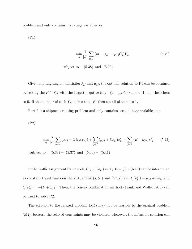
problem and only contains first stage variables yl:
(P1)
minyl
1
|L|∑j∈J
(mj + ξj,l − µj,lCj)Yj,l (5.42)
subject to (5.38) and (5.39)
Given any Lagrangian multiplier ξj,l and µj,l, the optimal solution to P1 can be obtained
by setting the P ’s Yj,l with the largest negative (mj + ξj,l−µj,lC) value to 1, and the others
to 0. If the number of such Yj,l is less than P , then set all of them to 1.
Part 2 is a shipment routing problem and only contains second stage variables xl:
(P2)
minxl
α
|L|∑a∈A
(xa,l − ba)ta(xa,l) +∑j∈J
(µj,l + θωj,l)vsj,l −
∑j∈J
(B + ωj,l)vdj,l (5.43)
subject to (5.33)− (5.37) and (5.40)− (5.41)
In the traffic assignment framework, (µj,l+θωj,l) and (B+ωj,l) in (5.43) can be interpreted
as constant travel times on the virtual link (j, Sd) and (Ss, j); i.e., tj(vsj,l) = µj,l + θωj,l and
tj(vdj,l) = −(B + ωj,l). Then, the convex combination method (Frank and Wolfe, 1956) can
be used to solve P2.
The solution to the relaxed problem (M5) may not be feasible to the original problem
(M2), because the relaxed constraints may be violated. However, the infeasible solution can
96

be used to generate feasible solutions (which provide upper bounds to the optimal objective
value) using Lagrangian Heuristics. Because (5.26) may be violated, y∗relax,l of different
scenarios l ∈ L may have different values. For each candidate location j ∈ J , count the
number of times that it is selected by a scenario, i.e., yj =∑l∈L
Y ∗relax,j,l. The candidate
locations are sorted by yj, and then are added to a set J∗ one by one from the ones with
the highest yj, until no locations with a positive yj left. Every time a j ∈ J is added to J∗,
we fix the values of y, i.e., set Yj,l = 1 for all l ∈ L if j ∈ J∗, and Yj,l = 0 otherwise. After
y is fixed, M2 becomes a capacitated shipment routing problem, and is solved using traffic
assignment algorithms (e.g., Frank and Wolfe, 1956; Daganzo, 1977(a, b)) for each scenario.
Let ZUB be the objective value of the current best solution we have so far. The obtained
solution becomes the new current best solution if its objective value is lower than ZUB. ZUB
serves as the upper bound of the objective value of M2, but it may not be a upper bound of
M1.
For any Lagrangian multipliers µ, ZD(µ) =∑l∈L
ZD,l(µ) is a lower bound to the optimal
value of M2. In order to find the best lower bound Z∗D = maxµ
ZD(µ), the conventional
subgradient method is applied to update multipliers µ over iteration steps (Fisher, 1981) as
is discussed in section 7.2.2.1.
If the optimal solutions of vsj are not all close to the built refinery capacities, there would
be a duality gap. In such cases, we further apply branch-and-bound (B&B) frameworks
discussed in section 3.3.2 to further improve the solution toward optimality.
97

5.1.3 Numerical Analysis
The Sioux Falls network shown in Figure 3.2(b) is adopted to test our proposed method-
ology, which has 24 vertices and 76 links in the transportation network. Both average supply
and demand, i.e., hs and hd, follow normal distributions with variance equals 1/5 of mean
(they are actually normal distributions truncated at point 0 because hs and hd cannot be
negative; the truncated tail has a probability of 2.9× 10⁻⁷ ). The differences between local
supply/demand and the average supply/demand, i.e., ∆hsi and ∆hdi′ follow standard normal
distributions (they are also truncated so that hi is non-negative). The BPR (U.S. Bureau of
Public Roads) function (3.14) is adopted as the link cost function.
First we need to decide the appropriate number of scenarios for using M2 to approximate
M1. We fixed the refinery build costs to be $50,000 per refinery, and run the algorithm for
different number of scenarios. The results are shown in Figure 5.3. In both (a) and (b),
the most left points are from the instance where there is only one scenario (i.e., |L| = 1 )
and the expected supply/demand is used for all farms/gas stations in this scenario. This is
actually the deterministic version of the problem. The other points in the figures are from the
instances where the scenarios are generated by Monte Carlo simulation. It can be seen that
when |L| is small, the best objective value obtained by the model fluctuates dramatically
across the problem instances. As |L| increases, the objective value gradually converges.
Theoretically when |L| tends to infinity the optimum objective value of M2 equals that of
M1. The converged value is very different from the case when one scenario with expected
supply/demand is used, which indicates that the deterministic model is not able to address
98
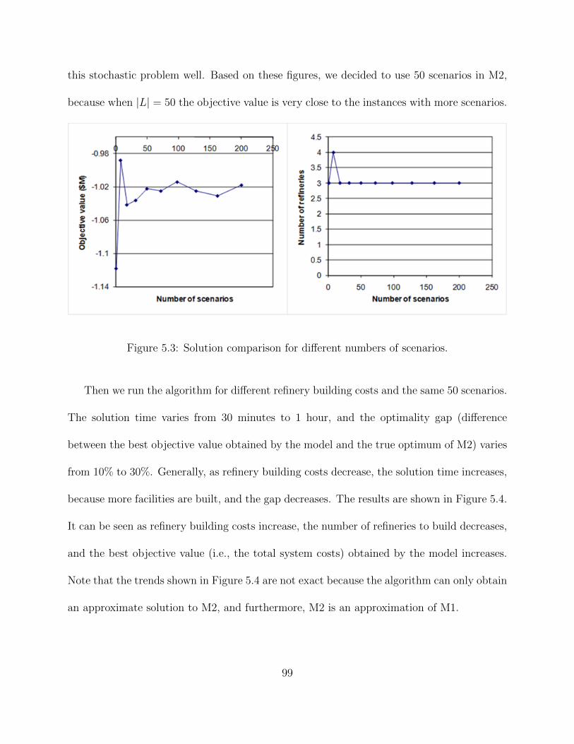
this stochastic problem well. Based on these figures, we decided to use 50 scenarios in M2,
because when |L| = 50 the objective value is very close to the instances with more scenarios.
Figure 5.3: Solution comparison for different numbers of scenarios.
Then we run the algorithm for different refinery building costs and the same 50 scenarios.
The solution time varies from 30 minutes to 1 hour, and the optimality gap (difference
between the best objective value obtained by the model and the true optimum of M2) varies
from 10% to 30%. Generally, as refinery building costs decrease, the solution time increases,
because more facilities are built, and the gap decreases. The results are shown in Figure 5.4.
It can be seen as refinery building costs increase, the number of refineries to build decreases,
and the best objective value (i.e., the total system costs) obtained by the model increases.
Note that the trends shown in Figure 5.4 are not exact because the algorithm can only obtain
an approximate solution to M2, and furthermore, M2 is an approximation of M1.
99

Figure 5.4: Solution comparison for different refinery building costs.
5.2 Reliable Biorefinery Location Design: An Illinois
Case Study
This sections focuses on designing bio-ethanol supply chains that not only operate effi-
ciently in the normal (i.e., disruption-free) scenario but also are able to provide sufficient
back-ups to minimize cost increase and negative social impacts under refinery disruptions.
Both discrete and continuous reliable location models are applied to the State of Illinois,
where (i) a significant amount of the nation’s biomass supply and bioethanol is produced,
and (ii) the state has already geared up toward a rapid expansion of bio-ethanol production
infrastructure.
We will first review the discrete reliable uncapacitated facility location model and La-
grangian relaxation based solution approach by Cui et al. (2010). This approach generally
can solve small to moderate instances to the exact optimality. Then we present a continuum
100

approximation approach based on the work by Cui et al. (2010) and Peng and Ouyang
(2010). This approach is suitable for large-scale instances with slow-varying conditions, and
can obtain approximated near-optimum solutions within much shorter time.
5.2.1 Discrete Model
Following the formulation of reliable uncapacitated facility location problem (RUFL)
in Cui et al. (2010), let J = 0, 1, · · · , |J | − 1 denote the set of candidate locations
where refinery facilities can be potentially built to collectively “serve” a set of farms, I =
0, 1, · · · , |I| − 1, where farm i ∈ I produces λi bushels of corn each year. Building a
refinery at location j ∈ J requires a prorated annual construction cost fj; transporting each
bushel of corn from farm i to refinery j imposes a yearly transportation cost dij.
A refinery, if built at candidate location j, is subject to a site-dependent disruption
probability qj. Assume refinery disruptions are independent and in each disruption scenario
(i.e., the pattern/combination of refinery disruptions), only functioning refineries can produce
bio-ethanol; the failed ones completely halt all their production lines. To hedge against such
disruption risks, each farm i is assigned to a subset of at most R ≥ 1 refineries. The refineries
in this subset are labeled with rank r = 0, 1, · · · , R − 1, which represents the priority for a
refinery to serve the demand from farm i. In other words, the rank-r refinery is the farm’s
(r+1)th choice for service. In the normal scenario (i.e., no refinery disruption), the rank-0
refinery serves the demand. If rank-0 refinery has failed, the rank-1 refinery takes over.
Such takeover continues based on the rank until all R assigned refineries have failed, and
then farm i lose service and incurs a penalty cost φi due to lost service and adverse social
101

impacts. For convenience, we incorporate this penalty cost into the model by defining a
preinstalled virtual “emergency” facility j = |J | with qJ = 0 that serves farm i at rank R
with transportation cost diJ = φi. For the simplicity of notation, we define J ′ = J⋃|J |.
The primary decision variables X := Xjj∈J determine where the refineries are built,
such that
Xj =
1, if a refinery is built at location j;
0, otherwise.
We also define two sets of auxiliary variables. The first set Y = Yijri∈I,j∈J ′,r=0,··· ,R
decides the assignment of farms to refineries; i.e.,
Yijr =
1, if refineryj is assigned to customeri at rankr;
0, otherwise.
The second set of variables P = Pijri∈I, j∈J ′,r=0,··· ,R specifies the probability of farm
i being served by refinery j at rank r. The objective is to determine the optimal refinery
locations and demand allocation plans to minimize the sum of facility construction cost
and total expected transportation cost across all disruption scenarios. The mathematical
program can be written as follows:
102

(RUFL)
minimizeX,Y,P
∑j∈J
fjXj +∑
i∈I
∑j∈J ′
∑R
r=0λidijPijrYijr (5.44)
subject to∑
j∈JYijr +
∑r
s=0YiJs = 1, ∀i ∈ I, r = 1, · · ·R (5.45)∑R−1
r=0Yijr ≤ Xj, ∀i ∈ I, j ∈ J (5.46)∑R
r=0YiJr = 1, ∀i ∈ I (5.47)
Pij0 = 1− qj, ∀i ∈ I, j ∈ J ′ (5.48)
Pijr = 1− qj∑k∈J
qk1− qk
Pik(r−1)Yik(r−1), ∀i ∈ I, j ∈ J ′, r = 0, 1, · · ·R (5.49)
Xj ∈ 0, 1, ∀j ∈ J (5.50)
Yijr ∈ 0, 1, ∀i ∈ I, j ∈ J ′, r = 0, 1, · · ·R (5.51)
This model can be solved by a customized Lagrangian relaxation (LR) algorithm that is
developed in Cui et al. (2010). The basic idea is to relax constraints (5.46) and add them
into the objective (5.44) with multipliers µ = µij. The relaxed RUFL model (RRUFL) is
as follows.
(RRUFL)
minimizeX,Y,P
∑j∈J
(fj −∑
i∈Iµij)Xj +
∑i∈I
∑j∈J
∑R
r=0(λidijPijr + µij)Yijr
+∑
i∈I
∑R
r=0λidiJPiJrYiJr (5.52)
subject to (5.45) and (5.47)− (5.51) (5.53)
103

Cui et al. (2010) showed that the RRUFL model can be simplified by approximating
variables Pijr into some fixed values. Let j0,j1, · · · , j|J |−1 be an ordering of all candidate
locations such that qj0 ≤ qj1 ≤ · · · ≤ qj|J |−1. Define βr =
∏r−1k=0 qjk, and replace the variable
probability Pijr with (1 − qj)βr. After this approximation, the problem can be solved in
linear time and provides a lower bound of the original objective (1.1) (but not necessarily
feasible). Then the solution of X is plugged back into model RUFL, and with fixed X values
the original RUFL can be easily solved to obtain a feasible solution (or an upper bound).
Note that the true optimum is always between the two bounds. After obtaining these two
bounds, the LR algorithm updates multipliers µ iteratively using the standard subgradient
method (Fisher 1981). In many cases, LR can close the optimality gap between the lower
and upper bounds and hence yield the exact optimal solutions after a few iterations. In case
a non-zero residual gap is present, the LR algorithm can be embedded into a branch and
bound (BB) procedure to effectively close the gap.
5.2.2 Continuous Approximation Model
Newell (1971) and Daganzo and Newell (1986) proposed a continuous approximation
(CA) method to efficiently solve a variety of logistics problems in a continuous setting. In our
context, we consider a 2-dimensional space S ⊂ R2, where the construction cost f , demand
density λ, penalty cost φ and disruption probability q are all continuous functions of point x ∈
S. The CA approach looks for the optimal continuous facility density, γ∗(x), or equivalently,
the optimal influence area size of a facility, A∗(x) = [γ∗(x)]−1, that minimizes the cost
per unit of area z (A(x), x) near location x. For the reliable uncapacitated facility location
104

problem, Cui et al. (2010) gave the following closed-form approximation of z (A(x), x); i.e.,
z (A(x), x) ≈ f(x)
A(x)+ φ(x)λ(x)[q(x)]R + λ(x)G (R, q(x))
√A(x).
Here, G (R, q) can be related to the expected travel cost in a homogeneous plane R2 (i.e.,
where all parameters f , λ, φ and q are independent of x). A close approximation of G(R, q)
is given by Li and Ouyang (2009):
G(R, q) ≈ 2
3√π
R∑r=0
(1− q)qr[(r + 1)3/2 − r3/2
].
For notation simplicity, we ignore argument x from now on (unless specified otherwise),
and (3) becomes:
z =f
A+ φλqR + λG(R, q)
√A
Given any neighborhood x, the optimal influence area size that minimizes (5) is:
A∗ ≈(
f
λG(R, q)
)2/3
and the corresponding cost per unit area is:
z∗ ≈ 2f 1/3(λG(R, q))2/3 + φλqR
Intuitively, the optimal total costs Z∗ and the optimal number of facilities n∗ are the inte-
105

grations of z∗ and γ∗ on S:
Z∗ =
∫S
z ∗ dx,
n∗ =
∫S
γ∗dx =
∫S
(A∗)−1dx.
5.2.2.1 Discrete Data and Location Design
In real-world applications, the CA approach needs to address several challenges. First, the
input data such as f , λ, φ and q may be defined (or available) only at a subset of discrete
points xk : k ∈ K in S (e.g., via spatial aggregation or sampling). Such discrete data could
be either (i) aggregated data; e.g., service demand λk, (ii) sampled data; e.g. penalty φk,
facility cost fk and disruption probability qk. These discrete data must be transformed
into continuous functions as input to the CA approach. Second, while the CA output γ∗
(e.g., facility density) has been shown repeatedly to provide very good estimates of the exact
optimal solution, it is not yet the actual solution that can be readily implemented. The CA
approach can be used to estimate system cost from discrete input (Peng and Ouyang, 2010).
The idea is to use nearest neighbor interpolation and Voronoi diagrams to convert the data
into continuous functions, taking the discrete points xk as Voronoi generators. Note that
when there are |K| generators, it takes O (|K| log |K|) time and O (|K|) memory space to
generate a Voronoi diagram (Fortune, 1986). Because the Voronoi diagram is only related to
data point location xk but not data values, it only needs to be constructed once for each
set xk. For example, let Sk be the set of Voronoi polygons, such that Sk is generated
from point xk, and⋃k∈KSk = S. The demand density can be simply estimated from the
106

discrete demand λk as follows,
λ(x) = λk/ |Sk| , ∀x ∈ Sk,∀k ∈ K,
The penalty cost, facility cost, and disruption probability can be estimated from the following
formulas:
φ(x) = φk, f(x) = fk, q(x) = qk, ∀x ∈ Sk,∀k ∈ K.
Sometimes the discrete points for demand information and facility information do not
overlap. For example, λk may be defined on xk : k ∈ K, while fj is defined on
yj : ∀j ∈ J . If the Voronoi polygons is constructed based on xk, f(x) could be defined
as
f(x) = fj(k), ∀x ∈ Sk, ∀k ∈ K,
where j(k) ∈ J is the index of location yj which is the closest to location xk; i.e., j(k) =
arg minj
‖yj − xk‖. The continuous functions generated from this method will have constant
values within each Voronoi polygon. As a result, the optimal cost per unit area z∗k and
optimal influence area size A∗k are also constant within this polygon. The total cost and
total facility number, Z∗ and n∗, can be approximated by
Z∗ ≈∑
k∈K|Sk| z∗k,
n∗ ≈∑
k∈K|Sk| /A∗k,
107

which can be solved in linear timeO (|K|).
To obtain near-optimum implementable solutions from the CA output, Ouyang and Da-
ganzo (2006) proposed a disk model to convert the continuous facility density function γ∗
into a set of discrete locations. After n∗ is estimated, the algorithm finds a set of n∗ round
disks which cover most of S. A disk centered at x0 has size A∗(x0). The locations of disk
centers are determined by exerting forces to disks and iteratively adjusting their positions.
Finally the disk centers are relocated to their nearest discrete candidate locations as the
built facilities. Interested readers are referred to Ouyang and Daganzo (2006) and Ouyang
(2007) for more details.
If the input data is discrete, Fan and Ouyang (2010) further propose a variant of the
disk model that (i) converts discrete data into continuous functions to calculate A∗, and (ii)
obtains a discrete feasible solution. A slightly different conversion algorithm is proposed for
(i), because in many cases a disk covers multiple demand points. The continuous functions
at x0 is dynamically updated based on information of all data points covered by the disk.
For example, for a disk centered at x0, with Sd being its circumscribed square and K(Sd)
being the set of discrete points covered by Sd. The farm demand density in this disk, λ(x0),
can be calculated as:
λ(x0) =
∑k∈K(Sd) λk
|Sd|,
where the total covered demand∑
i∈K(Sd) λk can be obtained by an orthogonal range counting
query in O (log |K|) time if data λk is stored in a range tree data structure (Luecker, 1978).
108

Other functions, such as φ(x0), can be estimated similarly by
φ(x0) =
∑k∈K(Sd) φk
|K(Sd)|,
while for f(x0) and q(x0), we could use
f(x0) = fj(x0) and q(x0) = qj(x0),
which each requires a nearest neighbor query. Such query takes O (log |K|) computation time
on average for randomly distributed discrete points if the data is stored in a kd-tree data
structure (Moore, 1991).
5.2.3 Data Preparation
This section describes the refinery infrastructure design case study for Illinois in the
year of 2022. In Illinois, surface water and aquifers are widely available, and the interstate
and local highways are easy to access in most counties (Tursun et al., 2008). Therefore we
assume that every centroid of the |J | = 102 Illinois counties is a candidate refinery location,
as shown in Figure 5.2.2.1(a). Ethanol refineries may be disrupted by site-independent
hazards such as power outages, operational incidents, labor actions. We assume that these
refinery disruptions are independent of each other. In addition, Illinois is covered by a dense
web of rivers (including primarily the Mississippi River and Illinois River) that pose major
flooding threats to refineries in Illinois, as shown in Figure 5.2.2.1(b). Most data we used is
the same as described in section 3.4 in chapter 3.
109

Figure 5.5: Input data for the Illinois case study.
We refer to Kang et al. (2008) to calculate the travel distance from each biomass supply
point to each candidate location along the shortest-distance path in the GIS highway network
provided by the Bureau of Transportation Statistics National Transportation Atlas Database
(RITA, 2008). Assuming that third-party carriers are used, the cost for shipping a bushel of
corn is $0.0016 per km (Mcvey et al. 2007). Since the CA model measures distances by the
Euclidean metric (instead of the highway network), all Euclidean distances are inflated by
a factor of 1.206 so that the average Euclidean distance is the same as the average highway
distance.
110

The probability for a refinery to be caught in a flood highly depends on the location
and geographical configuration. Therefore, we define the disruption probability as follows:
qj = q + q if county j is in a flood-prone area, or qj = q otherwise; the site-independent
component q counts for multiple common disruption hazards, and the site-dependent com-
ponent q represents local flooding probability. The value of probability q is estimated to be
0.05, based on refinery disruption records in California from 1997 to 2001 (Finizza, 2002).
However, very limited flooding frequency data are publicly accessible. We simply assume
that all counties along the Mississippi River and Illinois Rivers have relatively high risks of
flooding, and we will examine a range of q values in the sensitivity analysis.
We assume that a farm incurs a penalty cost after the three assigned refineries have all
been disrupted; i.e. R = 3. The penalty cost value (per unit biomass supply) is approxi-
mated by the net social cost due to the corresponding ethanol supply loss (Finizza, 2002).
Basically, refinery disruptions may lead to biomass supply loss and hence ethanol shortage.
For simplicity, we assume that the ethanol price is at equilibrium in an efficient market. In
case of disruptions, incremental supplies are sourced out of precautionary inventories and/or
from distant sources, which would raise local ethanol price. According to the 2002 California
Energy Commission (CEC) report, the price response at the time of a disruption is almost
instant. The mechanism of price rise to clear the market is in accordance with ethanol de-
mand elasticity. In the interim after the disruption and before the price return to normal,
the impact on the net social cost is contributed by a loss of consumer surplus (which is a
standard measure of societal benefit from an industry). In this sense, the penalty cost used
111

in this study can be interpreted as the net societal cost or the total loss of consumer surplus.
By applying the method and empirical data in Finizza (2002), we obtain a 5.96 total loss of
consumer surplus in the society. Therefore, the unit equivalent penalty cost φi, ∀i is roughly
φ:=15.
5.2.4 Numerical Results
This section presents numerical results of the case study. All solution algorithms are im-
plemented on a personal computer with 3.0 GHz CPU and 2GB memory. The LR algorithm
is coded in C++, while the CA approach is coded in MATLAB.
5.2.4.1 Impact of Refinery Disruptions
To understand the impact of refinery disruption on the bio-ethanol supply chain performance,
we run both the LR algorithm and the CA approach for three cases:
Case 1: all built refineries are robust and never fail (i.g., qj = 0, ∀j);
Case 2: all built refineries are subject to a homogeneous disruption probability qj =
q, forallj;
Case 3: all built refineries are also under the threat of flooding, so that the disruption
probability qj is heterogeneous across location j.
The results are shown in Table 5.1. It can be seen that LR and BB can obtain the
exact optimal solutions within half an hour. As the disruption probabilities increase, the
expected transportation cost increases significantly, while the normal transportation cost
reduces (which indicates that less biomass supply can be processed by its nearest refineries
112

because of disruption). As a result, the total cost rises considerably. Figure 5.2.4.1 and 5.2.4.1
show the impact of disruption risks on the optimal facility deployment. We see that cases 0
and 1 have the same location design, indicating that in this case, having q =0.05 alone is not
enough to affect the optimal locations of refineries. However, in case 3, the flooding threat
forces one refinery to move out of the flood-prone area (i.e., to avoid high disruption risk)
and another to be relocated (i.e., to back up the other relocated refinery), as indicated by
the arrows in Figure 5.2.4.1(b). When flooding risk is present (case 3), if we use the refinery
deployment from case 1 (or 2), the expected transportation cost across disrupted cases will
increase by 12% (although the total costs increase only by 0.37% due to the large fixed
investments). Therefore, facility disruption risks should not be ignored in supply network
design, especially when the disruption consequences are devastating.
Table 5.1: Summary of model solutions for different cases.
113

The CA model yields the estimated total costs Z∗ and the optimal number of refineries
n∗ almost instantaneously, while the errors are very small compared with the real optima.
The results of the disk model are obtained within 0.3 second, while the gap is about 10%.
This relatively large gap may be due to several reasons. First, the disk model is suitable
for large-scale problems with slow-varying conditions. However, the scale of our problem
instance is not large (only 102 data points) while the demand density (i.e., production of
corn) is spatially heterogeneous. It can be seen from Figure 5.2.4.1 that discrete model tends
to locate facilities to counties with high corn yield and low flood probabilities, even if they
are close to the geographical boundary. In contrast, the disk model generally is not able to
do so, especially when the location is very near the boundary, as shown in Figure 5.2.4.1. In
addition, the disk model uses the adjusted Euclidean distances, which may not be a close
approximation to the real highway distances. Finally, we use highly-aggregated biomass
production data and a small set of discrete candidate locations. If the biomass supply data
have a higher spatial resolution or if the facilities are allowed to be located anywhere in the
state, the disk model will be expected to have a better performance.
114

(a) (b)
Figure 5.6: LR and BB solution of refinery deployment.
Figure 5.7: CA disk model solution for case 3.
5.2.4.2 Sensitivity Analysis
In our case study, the refinery disruption probability and the penalty cost are estimated from
an empirical study in California. Those parameter values may not be suitable for Illinois due
to geographical, climate, and political differences. Hence, we apply the LR+BB algorithm
115

to conduct sensitivity analysis over a range of possible values. Figure 5.8 shows how the
total cost and the number of installations change with disruption probabilityq. We see that
the refinery number slightly increases with q (however, the refinery deployment may change
considerably). The total cost increases with q dramatically for larger q.
Figure 5.8: Sensitivity analysis on common disruption probability q (q = 0, φ = 15).
Figure 5.9 shows how the total cost and the number of installations change with the
flooding probability q. Again, both the refinery number and the total cost increase with q.
The cost increases faster for larger q. This strongly hints that facility disruption risks, if
present, should not be ignored in cost analysis.
116

Figure 5.9: Sensitivity analysis on flooding probability q (q = 5%, φ = 15).
Figure 5.10 shows how the penalty cost φ affects the results. Both the number of in-
stallation and the total cost increase sharply when φ is small. Once φ exceeds 1 (about
the maximum transportation cost per bushel), the influence diminishes. This is probably
because high penalty costs would force farmers to send out as much biomass as possible to
backup refineries even if they are far away, and as a result very little biomass supply actually
incurs the penalty cost.
117

Figure 5.10: Sensitivity analysis on penalty cost φ (q = 5%, q = 0).
118

Chapter 6
Biofuel Supply Chain Design underCompetitive Agricultural Land Useand Feedstock Market Equilibrium
6.1 Methodology
The competition between food and fuel use of feedstock supply is essentially about farm-
land allocation. Without loss of generality, we consider corn as the representative biofuel
feedstock and agricultural commodity in our context, because corn is one of the targeted
commodities in the food-versus-fuel debate. However, our proposed methodology can be
used to directly address land allocation among any food or bioenergy crops, such as the
second generation biomass feedstock.
6.1.1 Spatial Network Description and Notation
We consider a set of spatially distributed feedstock suppliers (i.e. farmers) I who provide
resources (i.e., corn) to a set of local markets M in a geographical region. Farmer i ∈ I
can produce a fixed total amount of corn gi per year. We also consider a set of candidate
biofuel refinery locations J for a biofuel company. We assume that the maximum capacity
119

of a refinery that can be built at location j ∈ J is cj, and the cost to build and operate
such a refinery can be prorated into annual equivalent cost of hj. Social-economic factors
(e.g. land price and availability, labor cost, etc) make hj vary across sites. We denote the
unit transportation cost ($/bushel) from farm i ∈ I to local market m ∈ M and candidate
refinery location j ∈ J as dij and dim, respectively. We assume that the unit price of
producing ethanol from one bushel of corn is pe(fJ), and it is determined by the inverse
demand function of total ethanol sold in the supply chain fJ := [fij]i∈I,j∈J with the production
cost for converting corn to ethanol included.
McNew and Griffith Mcnew and Griffith (2005) showed with empirical data that building
a biofuel refinery can raise the corn price in local markets and alter the spatial distribution of
price around the production and demand centers, as a direct result of the supply and demand
relationship. As illustrated in Figure 6.1, in an imperfectly competitive corn market, new
demand for biofuel feedstock shifts the joint corn demand curve to the right; with the supply
curve remaining the same, the equilibrium market price of corn increases from pm to p′m. As
a result, under market equilibrium, the total amount of corn supply for food (and livestock
feed) use decreases and the corn price increases (Pfuderer and Castillo, 2008).
In our analysis, we consider that a group of biofuel refineries can affect the market corn
price, and hence the system shows imperfectly competitive market behavior. Corn, as one of
major source of food and feed supply, is usually assumed to have inelastic demand (Schnepf,
2006; Pfuderer and Castillo, 2008). Thus, the impact of biofuel refinery on corn prices is
non-negligible, and we incorporate basic ideas of spatial equilibrium model with imperfectly
120

Figure 6.1: Demand and supply curve of corn under market equilibrium.
competitive market into the biofuel refinery location modeling framework (Gallagher et al.,
2003). On the other hand, the price at a certain refinery location depends on the biofuel
manufacturer’ offer, but it is also closely related to the local market price, since the biofuel
manufacturer needs to bid for corn supply from farmers. Hence, the site-specific corn price
at refinery locations is another important decision for a biofuel company in its supply chain
design 1.
The decision variables of the problem are as follows:
x := (xj)j∈J : binary refinery location variables, where xj = 1 if location j is selected
to build a refinery or xj = 0 otherwise;
1Since we focus on local bio-refinery investment, the global market price of the agricultural commodityis not likely to be affected (e.g., due to the addition of a few bio-refineries). Hence, for simplicity importsand exports of agricultural commodities are not considered in this study. In fact, these factors could beaddressed in our model by considering additional sources of supply or demand near the boundary of thestudy area.
121

pJ := (pj)j∈J : corn prices offered at candidate refinery locations;
fM := [fim]i∈I,m∈M : corn flow from farms to local markets;
fJ := [fij]i∈I,j∈J : corn flow from farms to candidate refinery locations;
q := (qm)m∈M : the total amount of corn supplied to local markets;
pM := (pm)m∈M : market equilibrium prices of corn at local markets.
6.1.2 Noncooperative Stackelberg Game Formulation
Consider a non-corporative scenario, where a biofuel company constructs building refiner-
ies in multiple locations and offers certain prices to procure feedstock, and a set of spatially
distributed farmers reacts accordingly to maximize their individual profits. The problem
can be regarded as a Stackelberg leader-follower game with facility location decisions and
formulated as a bilevel DC-MPEC problem.
We assume that each farmer i ∈ I with a fixed total yield gi has the option to ship
and sell corn to local grain markets or to nearby refineries, but the farmers themselves bear
the transportation cost. The profit of farmer i ∈ I under its corn flow decision vector
fi ,(fik
)k∈M∪J
2 is
π ( fi ) =∑m∈M
( pm − dim ) fim +∑
j∈J :xj=1
( pj − dij ) fij . (6.1)
Here, it is implicitly assumed that fi do not affect the costs that are associated with pro-
ducing corn, and these costs are excluded from π ( fi ). Therefore, only prices pm, pj and
2The hat in fi and fik is used to distinguish the decisions of farmer i from those of other farmers in I.
122

transportation cost dim, dij affect farmer i’s unit profit from selling corn (to local markets or
refineries). The corn price at local market m ∈ M can be estimated by corn demand curve
pm = ψm(fM), where the total amount of corn supplied to local market m is qm :=∑
i∈I fim.
Given refinery locations and corn price offers, the land use optimization problem for a
generic farmer i ∈ I is as follows, where fi′j for i′ 6= i is exogenous to this optimization:
maximizefi≥ 0
∑m∈M
( pm − dim ) fim +∑
j∈J :xj=1
( pj − dij ) fij (6.2)
subject to∑
k∈M∪J
fik ≤ gi (6.3)
and fij +∑i′ 6=i
fi′j ≤ cj xj ∀ j ∈ J. (6.4)
The objective function in (6.2) maximizes the profit for individual farmer i ∈ I. Constraint
(6.3) enforces that outbound corn flow from farm i should be no more than the corn yield gi
of that farm. Constraints (6.4) ensure that corn can only be shipped and sold to candidate
location j only if there is a refinery built at j and the total flow throughput should not
exceed the capacity of the refinery.
In biofuel supply chains, the biofuel manufacturer makes investment decisions to maxi-
mize the total profit. The decisions include the number and location of refineries and the
price offers to the farmers for feedstock supply. We formulate the optimization problem for
123
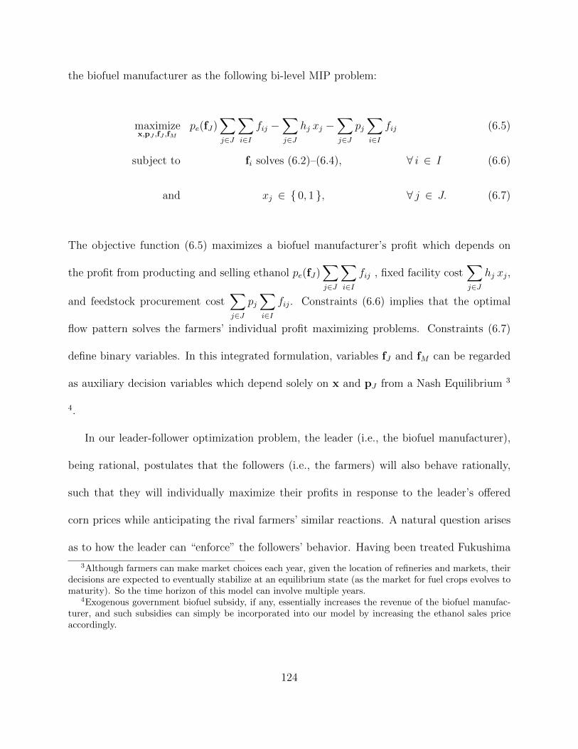
the biofuel manufacturer as the following bi-level MIP problem:
maximizex,pJ ,fJ ,fM
pe(fJ)∑j∈J
∑i∈I
fij −∑j∈J
hj xj −∑j∈J
pj∑i∈I
fij (6.5)
subject to fi solves (6.2)–(6.4), ∀ i ∈ I (6.6)
and xj ∈ 0, 1 , ∀ j ∈ J. (6.7)
The objective function (6.5) maximizes a biofuel manufacturer’s profit which depends on
the profit from producting and selling ethanol pe(fJ)∑j∈J
∑i∈I
fij , fixed facility cost∑j∈J
hj xj,
and feedstock procurement cost∑j∈J
pj∑i∈I
fij. Constraints (6.6) implies that the optimal
flow pattern solves the farmers’ individual profit maximizing problems. Constraints (6.7)
define binary variables. In this integrated formulation, variables fJ and fM can be regarded
as auxiliary decision variables which depend solely on x and pJ from a Nash Equilibrium 3
4.
In our leader-follower optimization problem, the leader (i.e., the biofuel manufacturer),
being rational, postulates that the followers (i.e., the farmers) will also behave rationally,
such that they will individually maximize their profits in response to the leader’s offered
corn prices while anticipating the rival farmers’ similar reactions. A natural question arises
as to how the leader can “enforce” the followers’ behavior. Having been treated Fukushima
3Although farmers can make market choices each year, given the location of refineries and markets, theirdecisions are expected to eventually stabilize at an equilibrium state (as the market for fuel crops evolves tomaturity). So the time horizon of this model can involve multiple years.
4Exogenous government biofuel subsidy, if any, essentially increases the revenue of the biofuel manufac-turer, and such subsidies can simply be incorporated into our model by increasing the ethanol sales priceaccordingly.
124

(2011); Krawczyk (2007) to a certain extent in the context of a “generalized Nash game”
via a penalty approach and a price mechanism, this enforcement issue in the present bilevel
context is not as straightforward as in the situation of the references; for one thing, the
treatment there is aimed at the “coupled constraints” (6.4) which are known to be the
source of computational challenges for solving such games in general. In the leader-follower
formulation as a bilevel optimization problem, the leader makes no attempt to enforce the
followers’ responses; instead, the leader postulates such responses and includes them as
constraints in the leader’s optimization. The investigation of the leader’s enforcement of the
followers’ responses is worth further study but is outside the scope of this study.
6.1.3 Solution Approach
We further assume that the corn demand functions pm = ψ(qm), ∀m ∈ M follow a
special case of linear inverse demand functions, i.e., pm = ψ(qm) = a1m − a2m
∑i∈I
fim, where
coefficients a1m > 0 and a2m > 0 are respectively the intercept and slope of the inverse
demand function for any m ∈ M . The Stackelberg game model (6.5)–(6.7) can then be
125

formulated as the following bi-level mixed-binary integer program:
maximizex,pJ ,fJ ,fM
pe(fJ)∑j∈J
∑i∈I
fij −∑j∈J
hj xj −∑j∈J
pj∑i∈I
fij
subject to xj ∈ 0, 1 , ∀ j ∈ J
and for all i ∈ I : anticipating f−i, pJ , and x,
fi ∈ argmaxfi≥ 0
∑m∈M
[a1m − a2m
(fim +
∑i′ 6=i
fi′m
)− dim
]fim
+∑
j∈J :xj=1
( pj − dij ) fij
subject to
∑k∈M∪J
fik ≤ gi
and fij +∑i′ 6=i
fi′j ≤ cj xj ∀ j ∈ J.
(6.8)
Subsequently, we will show that the sum of bilinear terms∑j∈J
pj∑i∈I
fij in the objective
function of (6.8) can be rewritten as a convex quadratic function of the decision variables;
see (7.12), similar to the derivation in Hobbs et al. (2000).
Shared by all the farmers, the coupled constraints∑i∈I
fij ≤ cjxj for all j ∈ J is satisfied
at any solution of the farmers’ Nash Equilibrium problem. By the boundedness constraints∑k∈M∪J
fik ≤ gi, whose Lagrange multiplier we denote λi, it follows that the farmers have
common multipliers for the former coupled constraints, which we denote ρj for j ∈ J . Writ-
ing down the Karush-Kuhn-Tucker (KKT) optimality conditions of farmer i’s optimization
126

problem, we deduce, for all i ∈ I:
0 ≤ fim ⊥ dim − a1m + a2m
(fim +
∑i′∈I
fi′m
)+ λi ≥ 0, m ∈ M
0 ≤ fij ⊥ dij − pj + λi + ρj ≥ 0, j ∈ J such that xj = 1
0 ≤ λi ⊥ gi −∑m∈M
fim −∑
j∈J :xj=1
fij ≥ 0
0 ≤ ρj ⊥ cj −∑i∈I
fij ≥ 0, j ∈ J such that xj = 1
0 = fij j ∈ J such that xj = 0.
Without loss of generality, we may assume that
a1m ≥ mini∈I
dim, ∀m ∈ M.
Otherwise, if a1m < mini∈I
dim for some market m, then fim = 0 for all i ∈ I, implying that no
farmer will sell to that market m. Under this assumption, the above KKT conditions yield
λi ≤ max
maxm∈M
( a1m − dim ) , maxj∈J :xj=1
( pj − dij ) , 0
, ∀ i ∈ I, (6.9)
which clearly holds if λi = 0; whereas if λi > 0, then there must exist either an m ∈M such
that fim > 0 or a j ∈ J with xj = 1 such that fij > 0. Thus (6.9) always holds, which yields
a valid bound of the multipliers λi in terms of the (variable) locational prices pj offered by
the biofuel manufacturer and the nonnegative constant maxm∈M
( a1m − dim ). In order to derive
127

a constant bound of these multipliers, we first observe that from the same KKT conditions,
we can derive
∑j∈J
pj∑i∈I
fij =∑i∈I
∑m∈M
fim dim +∑
j∈J :xj=1
fij dij + gi λi
+
∑j∈J :xj=1
cj ρj +∑m∈M
∑i∈I
[a2m
(fim +
∑i′∈I
fi′m
)− a1m
]fim,
(6.10)
which expresses, for fixed x, the (nonconvex) sum of products∑j∈J
pj∑i∈I
fij in terms of the
sum of a convex (since a2m > 0) quadratic function of the sale variables fim and a linear
function of the multipliers λi and ρj. Next we derive an upper bound for the sum∑j∈J
pj∑i∈I
fij,
which we will use to bound the multipliers. Specifically, since x = 0, yielding fij = 0 for
all i ∈ I and j ∈ J , is always feasible, it follows that an optimal solution of the biofuel
manufacturer’s profit must be non-negative; thus,
pe(fJ)∑j∈J
∑i∈I
fij −∑j∈J
hj xj −∑j∈J
pj∑i∈I
fij ≥ 0.
This implies, ∑j∈J
pj∑i∈I
fij ≤ pe(fJ)∑j∈J
∑i∈I
fij −∑j∈J
hj xj.
128

Hence,
∑i∈I
gi λi +∑
j∈J :xj=1
cj ρj
≤ pe(fJ)∑j∈J
∑i∈I
fij −∑j∈J
hj xj +∑m∈M
∑i∈I
[a1m − a2m
(fim +
∑i′∈I
fi′m
)]fim
≤ ∆ , maximumfi≥ 0;xj ∈0,1
pe(fJ)
∑j∈J
∑i∈I
fij −∑j∈J
hj xj
+∑m∈M
∑i∈I
[a1m − a2m
(fim +
∑i′∈I
fi′m
)]fim
subject to∑
k∈M∪J
fik ≤ gi, ∀ i ∈ I
and∑i∈I
fij ≤ cj xj, ∀ j ∈ J.
Hence, for each j ∈ J with xj = 1, we obtain the following bound 5 for pj:
pj ≤ ρj + mini∈I
(λi + dij ) ≤ ∆
cj+ min
i∈I
(∆
gi+ dij
).
5This bound can also be used for pj corresponding to xj = 0 because such a pj has no effect on the innerand outer objective functions.
129

Therefore, for all i ∈ I,
λi ≤ min
[∆
gi, max
maxm∈M
( a1m − dim ) , maxj∈J :xj=1
( pj − dij ) , 0
]
≤ min
[∆
gi, max
maxm∈M
( a1m − dim ) , maxj∈J :xj=1
(∆
cj+ min
i∈I
(∆
gi+ dij
)− dij
), 0
], λi.
(6.11)
Thus to upper bound the multipliers and prices, it suffices to solve a mixed concave quadratic
maximization integer program to obtain the scalar ∆ (assuming that pe(fJ) is a linear func-
tion of the total sales∑j∈J
∑i∈I
fij with nonpositive slope); from ∆ the desired bounds for λi,
ρj and pj can be obtained readily. The resulting bound could presumably be tightened by
refining the above derivations.
Formulation as a mixed integer program. We want to bound the sum fim +∑i′∈I
fi′m
from the above. If fim > 0, then
dim − a1m + a2m
(fim +
∑i′∈I
fi′m
)+ λi = 0,
which yields,
fim +∑i′∈I
fi′m ≤a1m − dim
a2m
.
If fim = 0, then
fim +∑i′∈I
fi′m ≤∑i 6=i′∈I
gi ′ .
130

Also, we have
fim +∑i′∈I
fi′m ≤ gi +∑i′∈I
gi ′ .
Hence,
fim +∑i′∈I
fi′m ≤ min
max
(a1m − dim
a2m
,∑i 6=i′∈I
gi ′
), gi +
∑i′∈I
gi ′
, f sum
im (6.12)
Moreover, for all j ∈ J with xj = 1, we have
λi + ρj ≤∆
min ( gi, cj ), ξij (6.13)
Utilizing (7.12), (7.15), (6.12), and (7.19), we obtain a mixed integer programming for-
mulation of the Stackelberg game (6.8):
131

maximizex,pJ ,fJ ,fM
pe(fJ)∑j∈J
∑i∈I
fij −∑j∈J
hj xj −∑i∈I
∑m∈M
fim dim +∑
j∈J :xj=1
fij dij
−∑i∈I
gi λi −∑
j∈J :xj=1
cj ρj −∑m∈M
∑i∈I
[a2m
(fim +
∑i′∈I
fi′m
)− a1m
]fim
subject to xj ∈ 0, 1 , ∀ j ∈ J
si ∈ 0, 1 , ∀ i ∈ I
yj ∈ 0, 1 , ∀ j ∈ J
zik ∈ 0, 1 , ∀ i ∈ I, ∀ k ∈ M ∪ J
and for all i ∈ I, all m ∈ M , and all j ∈ J :
0 ≤ fim ≤ gi zim
0 ≤ dim − a1m + a2m
(fim +
∑i′∈I
fi′m
)+ λi
≤(dim − a1m + a2m f
sumim + λi
)( 1− zim )
0 ≤ fij ≤ cj zij
0 ≤ dij − pj + λi + ρj ≤[dij + ξij
]( 1− zij )
0 ≤ λi ≤ λi si
0 ≤ gi −∑
k∈M∪J
fik ≤ gi ( 1− si )
0 ≤ ρj ≤∆
cjyj
0 ≤ cj xj −∑i∈I
fij ≤ cj ( 1− yj )
0 ≤ pj
and for all j ∈ J,
xj + yj ≥ 1
xj ≥ zij, ∀ i ∈ I.
(6.14)
132

The upshot of the above derivation is that the original bi-level DC-MPEC formulation
(6.8) of the Stackleberg game is transformed into an equivalent mixed concave quadratic
maximization integer programming problem (7.21); the latter can be directly solved by
existing MIQP solvers (e.g., CPLEX).
6.1.4 A Cooperative Model
An alternative scenario is the case where farmers and the emerging biofuel industry
cooperate to achieve system optimum for the entire supply chain. This scenario could happen
for example if the farms are acquired by the industry and become its subsidiaries. To this
end, we formulate an mixed-integer nonlinear programming model that optimizes biorefinery
locations taking into consideration the bidirectional effect on suppliers’ profit-maximizing
strategies, as follows:
maximizex,pJ ,fI
pe(fJ)∑j∈J
∑i∈I
fij −∑j∈J
hj xj −∑
j∈J :xj=1
dijfij+
∑i∈I
∑m∈M
(ψm(fM)− dim) fim
subject to∑
k∈M∪J
fik ≤ gi, ∀ i ∈ I
∑i∈I
fij ≤ cj xj, and xj ∈ 0, 1 , ∀ j ∈ J.
(6.15)
The objective function maximizes the net profit of the farmers and the biofuel industry.
Note that the industry’s feedstock procurement cost and the farmers’ revenue from sales
to the industry have cancelled out. The constraints are similar to those described in the
133

noncooperative model.
6.2 Numerical Example
6.2.1 Data Preparation
The proposed models and solution approaches are used to design a small scale corn-based
biofuel supply chain for the State of Illinois (a major agricultural state producing 40% of
the corn ethanol consumed in the United States in 2008). The centroids of the top corn
production counties (based on 2008 production data) are selected to represent individual
farms (Kang et al., 2010; Khanna et al., 2008). The candidate bio-refinery locations are
selected based on accessibility to major interstate highways (Kang et al., 2010; Bai et al.,
2011b), and a set of local grain markets are considered based on proximity to the farms.
The transportation distances are obtained from the National Transportation Atlas Database
(RITA, 2008), while the transportation cost rate is assumed to be $0.0035 per bushel per
mile by semi-trailers (Mcvey et al., 2007). Figure 6.2 is an illustration of one of the networks
with 10 farms, 10 candidate refinery locations and 10 local grain markets.
134

Figure 6.2: An example of Illinois network
In the case study, we assumed a 10-year service life of biorefineries, and the fixed cost
parameter for building refineries is amortized into annual cost to be consistent with other cost
components. The refinery capacity at all candidate locations can be up to 200 million gallons
per year (MGY) and the prorated refinery construction cost is roughly 18 million dollars per
100 MGY capacity per year (Ellinger, 2008). We use a constant ethanol production profit
at pe ≡ $1.42 per gallon (Brown et al., 2007; Gehlhar et al., 2010) and the corn-to-ethanol
conversion factor of 2.8 gallon per bushel (Chen et al., 2010). The corn demand curve at
each local market is assumed linear and static (Karp and Mccalla, 1983), with a1m = $4.4
per bushel and a2m = $0.04 per million bushels annually for all m ∈ M . These coefficients
are approximated based on the corn price information in (Anderson and Coble, 2010) and
USDA AMS cash price report (USDA-AMS, 2010).
Table 6.1 summarizes some computational results for cases with varying refinery capac-
135
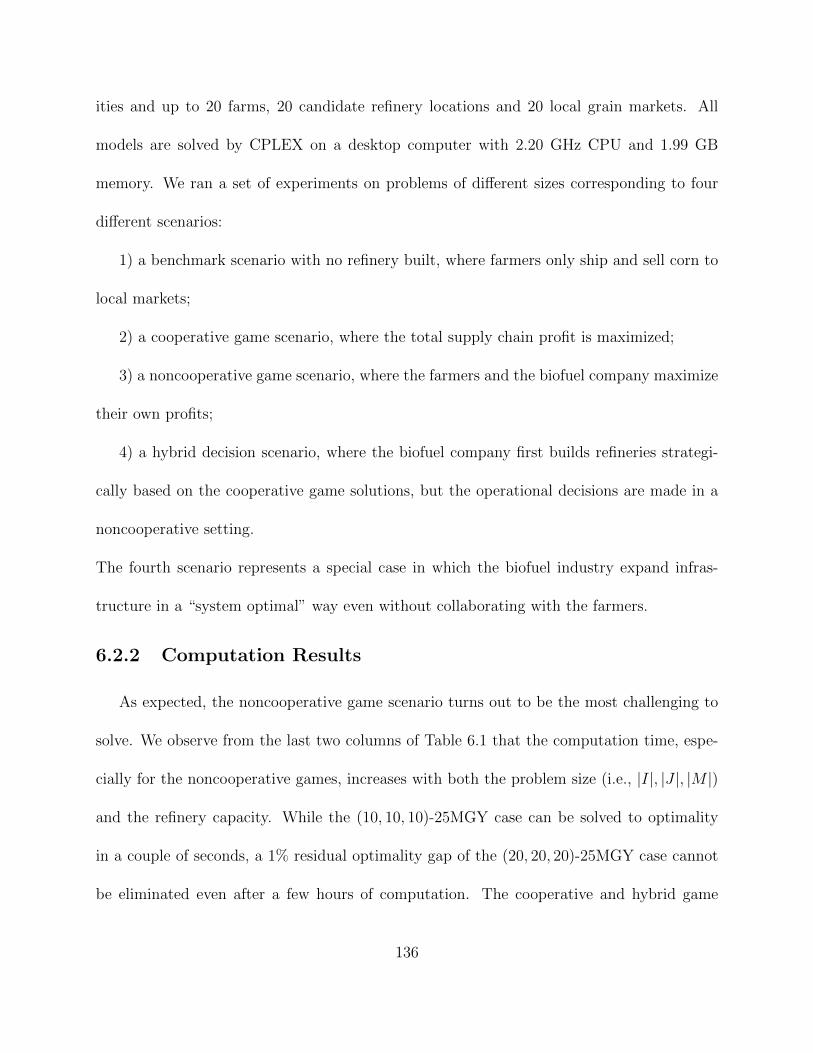
ities and up to 20 farms, 20 candidate refinery locations and 20 local grain markets. All
models are solved by CPLEX on a desktop computer with 2.20 GHz CPU and 1.99 GB
memory. We ran a set of experiments on problems of different sizes corresponding to four
different scenarios:
1) a benchmark scenario with no refinery built, where farmers only ship and sell corn to
local markets;
2) a cooperative game scenario, where the total supply chain profit is maximized;
3) a noncooperative game scenario, where the farmers and the biofuel company maximize
their own profits;
4) a hybrid decision scenario, where the biofuel company first builds refineries strategi-
cally based on the cooperative game solutions, but the operational decisions are made in a
noncooperative setting.
The fourth scenario represents a special case in which the biofuel industry expand infras-
tructure in a “system optimal” way even without collaborating with the farmers.
6.2.2 Computation Results
As expected, the noncooperative game scenario turns out to be the most challenging to
solve. We observe from the last two columns of Table 6.1 that the computation time, espe-
cially for the noncooperative games, increases with both the problem size (i.e., |I|, |J |, |M |)
and the refinery capacity. While the (10, 10, 10)-25MGY case can be solved to optimality
in a couple of seconds, a 1% residual optimality gap of the (20, 20, 20)-25MGY case cannot
be eliminated even after a few hours of computation. The cooperative and hybrid game
136

instances can all be solved quite efficiently.
Table 6.1: Computation results for the Illinois case study
The optimal design of biofuel supply chain (e.g., the number of refineries) and the corre-
sponding total system profit (for both farmers and industry) vary significantly across cooper-
ative versus noncooperative scenarios. In most cases the biofuel industry tends to construct
more refineries when the farmers are cooperative, and as a result, the system incurs higher
biofuel production, lower transportation cost, and an increase in total profit by about 13-
30%. This observation underscores the potential economic benefits from farmer-industry
cooperation. The whole system could be better off if we can design effective pricing and in-
centive mechanisms for the industry to drive the noncooperative farmers toward cooperation.
As such, the industry will achieves higher profit while part of the gain is shared equitably
with the farmers.
We also observe that the introduction of the biofuel industry has a significant impact on
137

the agricultural business (in contrast to the “no refinery” case). After the refineries are built,
some of the farmers are willing to sell part of their corn yield to nearby refineries rather
than local grain markets, sometimes even when transportation costs are higher, because
the refineries may offer even higher corn prices. Meanwhile, the corn prices in local food
markets may also be significantly boosted due to supply reduction. For example, for the
(20, 20, 20)-25MGY case, our computation shows that the average market price of corn
at equilibrium increases by roughly 6.2% and 24.3% in the cooperative and noncooperative
scenarios, respectively. These effects are obviously in favor of the farmers, but there are
also socio-economic and environmental cautions, e.g., increase in transportation distance
and GHG emission. For example, the results show a general increase in transportation cost
when the biofuel industry is introduced (e.g., $92-$125 million for the (20, 20, 20)-25MGY
case), which has mainly resulted from the larger quantity of corn yield shipped and sold
to farther outlets (due to higher market prices). These findings could provide insights for
further studies on the GHG emissions and energy consumption involved in biomass logistics.
138

(a) (b)
Figure 6.3: Supply/demand pattern of optimal solutions in the (10, 10, 10)-50MGY case
These computational results also demonstrate the fact that the biofuel industry does
have the capability to attract a significant amount of farmland for energy production, which
in turn influences the food markets. With higher feedstock prices at refineries, a significant
portion of agriculture land is allocated by the farmers to grow energy biomass. In our exam-
ples, for the (20, 20, 20)-25MGY case, almost half (44%) of the farmland is used for energy
production in the noncooperative game scenario. When farmers and industry cooperate, an
even higher percentage (86%) of land is allocated to energy. The supply/demand pattern
and transportation distances of a (10, 10, 10)-50MGY case are shown in Figure 6.3.
Finally, the results for the hybrid decision scenario have also shown that in most cases by
building refineries in a “system optimal” way even without cooperation with farmers, biofuel
manufacturers may increase the total profit of the whole supply chain while sacrifice a small
part of its own benefit. In this case, potentially all parties could be better off compared with
139

the pure noncooperative scenario if certain leverages for benefit reallocation are used.
6.2.3 Social Welfare Estimation
The solutions of our models have provided implications on how biofuel supply chain
profitability and the impacts on local feedstock markets vary under different business part-
nership scenarios. Our model results can be further utilized to analyze social welfare; e.g.,
by estimating the social surpluses as follows:
Social welfare = (CS + PS)biofuel + (CS + PS)biomass feedstock
where CS and PS stand for consumer and producer surpluses respectively.
In this case study, we assume that the biofuel manufacturer is a price taker in the ethanol
market and the ethanol price remains constant. As such, the biofuel consumer surplus is
identical in all scenarios. The producer surplus of both biofuel and biomass feedstock equals
respectively the net profits of the biofuel manufacturer and farmers. Consumer surplus of
biomass feedstock can be computed by∑m∈M
∫ q∗m
0
(ψ(qm)− p∗m) dqm, where p∗m and q∗m are
respectively the equilibrium supply and price in food market m ∈M . The social welfare for
each scenario is shown in Table 6.2.
140

(|I|, |J|, |M|)Refinery capacity
Scenario PS of biofuel CS of biomass PS of biomass Social Welfare
(10, 10, 10) 25 MGY no biofuel 0 541 1130 1671(10, 10, 10) 25 MGY cooperative 2110 8 191 2309(10, 10, 10) 25 MGY noncooperative 263 190 1580 2033(10, 10, 10) 25 MGY hybrid 249 187 1581 2017(10, 10, 10) 50 MGY no biofuel 0 541 1130 1671(10, 10, 10) 50 MGY cooperative 2106 6 171 2283(10, 10, 10) 50 MGY noncooperative 248 194 1576 2018(10, 10, 10) 50 MGY hybrid 239 186 1586 2011(10, 10, 10) 100 MGY no biofuel 0 541 1130 1671(10, 10, 10) 100 MGY cooperative 2080 8 184 2272(10, 10, 10) 100 MGY noncooperative 227 199 1565 1991(10, 10, 10) 100 MGY hybrid 221 193 1620 2034(20, 15, 10) 25 MGY no biofuel 0 575 1162 1737(20, 15, 10) 25 MGY cooperative 3599 10 203 3812(20, 15, 10) 25 MGY noncooperative 831 489 1929 3249(20, 15, 10) 25 MGY hybrid 817 477 1947 3241(20, 15, 10) 100 MGY no biofuel 0 575 1162 1737(20, 15, 10) 100 MGY cooperative 3545 8 132 3685(20, 15, 10) 100 MGY noncooperative 780 519 1879 3178(20, 15, 10) 100 MGY hybrid 774 495 2344 3613(20, 20, 20) 25 MGY no biofuel 0 287 1148 1435(20, 20, 20) 25 MGY cooperative 3572 4 167 3743(20, 20, 20) 25 MGY noncooperative 855 251 1852 2958(20, 20, 20) 25 MGY hybrid 849 273 1903 3025
Table 6.2: Social welfare for all scenarios (million $/year)
In all cases, our results indicate that biofuel production, regardless of the business part-
nerships, generally increases the net social welfare compared to the no-refinery status quo.
This supports our incentive to develop an economically feasible biofuel industry. However,
the consumer surplus of corn significantly decreases because of biofuel production, from which
we can say that its impact on food market is substantial. Furthermore, it is not a surprise to
see that the cooperative scenario generates highest social welfare since this scenario implies
system optimum. Note that under this scenario, the surplus of the manufacturer is much
higher than that of farmers. This is because our model does not consider a “compensation”
mechanism that re-distributes the manufacturer’s profit gain to the farmers.
141

Chapter 7
Biofuel Supply Chain Design underFarmland Use Regulations
Large-scale production of energy crops has direct impacts on the U.S. economy. Biofuel
production has been believed as one of the major drivers behind the price increase of corn and
other down-stream food products in the US in recent years, and thus is concerned as a risk of
the nation’s food security. According to Oladosu et al. (2011) and IAPC (2012), the share of
corn being used for ethanol production has increased up to more than 40% in 2010 compared
to only 10% in 2004/2005, and corn prices reached record high levels in 2010/2011 (e.g., more
than 3.5 times as high as those in 2005). In light of the ever increasing food demand and food
price, the development of a biofuel supply chain is concerned to have far-reaching impacts
on food security for a growing global population, and impose challenges to the resource
supply systems. The expected increase in U.S. biofuel consumption induces further demand
for bio-energy crops including first and second generations of biomass. The new outlet for
these agricultural commodities results in competition between food and energy use, which
essentially is due to limited farmland use. In other words, the impact of biomass feedstock
production on the food market is ultimately due to the competition for farmland allocation
142

between conventional food crops and energy crops. The potential impacts on farmland use
include the direct land use change (i.e., conversion of land from some other use directly
into biomass production) and indirect land use change (i.e., a cascade of land-use off-set
elsewhere) (USDA, 2011a). These impacts make it critical for policy makers to regulate the
agricultural industry to protect the food supply. The land allocation between food and fuel
have profound impacts on the agricultural economy, food security domestically and globally
and thus is a pressing problem to be taken into account on the question how the biofuel
industry should be expanded. As such, it is timely to study possible regulations/policies on
the current and marginal land use in prevention of future food crisis.
In this chapter, we explore possible governmental regulation scenarios on farmland use,
and model it into the biofuel manufacturer’s supply chain problem. We propose a Stackelberg-
Nash game framework with land use constraints to model the competitive supply chain design
problem under governmental land use regulation. However, it is hard to impose these con-
straints directly on farmers, so we focus on studying how to implement these regulations on
farmers’ land use choice to reach the government’s goal in total energy land use reduction.
To design a mechanism that provides them with incentives to limit energy crop production,
we propose a cap and trade system which is shown to theoretically attain the same effect as
directly imposing the land use constraints.
Our proposed Stackelberg-Nash game models on biofuel supply chain design fall into the
category of discretely constrained mathematical program with equilibrium constraints (DC-
MPEC). DC-MPECs have not been extensively studied in literature, and to date there is few
143

approaches that can efficiently solve such problems or is applicable to large scales problems.
Another major contribution of this chapter is the utilization of the existing theory of the
LR algorithm and recent advances on MPECs to develop a customized solution approach
to solve the competitive supply chain design problem, and the methodological exploration
to tackle this novel class of DC-MPEC problems. Specifically, we develop two adaptive
relaxation algorithms with Lagrangian relaxation (LR) and linear program (LP) relaxation to
decompose the DC-MPEC problem into simpler subproblems. Both algorithms are shown to
be effective in solving the proposed DC-MPEC model for even large scale instances. Finally,
we apply our model and solution approach to a numerical example in Illinois, and conduct
a before and after analysis to illustrate the impact of the proposed land use regulation
on the biofuel supply chain design and regional land use pattern. The proposed cap and
trade system is found to improve the total benefit for both the food and fuel supply chains.
Managerial insights can also be drawn for policy makers to maximize the social benefit and
for biofuel companies to design a sustainable biofuel supply chain.
7.1 Land Use Regulation Models
In this section, we model the agricultural regulations by limiting land use for energy pur-
pose to protect the food supply chain from losing excessive farmland to the energy industry.
We propose two competitive biofuel supply chain design models for a biofuel company, in
which the biofuel company needs to establish a new biofuel supply chain by building biore-
fineries anticipating farmers land use at market equilibrium. We first propose a base model
with land use constraints, and later we will propose an equivalent model which implements
144

the land use constraints to farmers through a cap and trade mechanism.
We follow the notation and modeling framework in our previous chapter, so we will focus
on integrating the land use constraints into the supply chain design model. Suppose the
biofuel company can select refinery locations out of a set J of candidate locations, and we
denote this decision by binary decision variable xj ∈ 0, 1,∀j ∈ J . Building a refinery
at location j ∈ J of capacity cj incurs a fixed cost hj. Another decision variable for the
company is the price offer to farmers for procuring biomass feedstock at each refinery, which
we denote as pj, j ∈ J . There are also a set I of farmers and a set M of food markets (e.g.,
local grain elevators, ports of exportation) discretely located in the study region. We assume
that farmer i ∈ I owns initially gi units of farmland and the total available land (including
marginal land) is L, and each farmer faces a farmland allocation problem. Specifically, in this
problem, variables fim, fij, and ri for all j ∈ J,m ∈M are used to denote farmer i’s decision
variables on how much land to grow and sell food crops to each market and energy crops to
refineries, as well as to enroll in the CRP respectively. As such, the total land that farmer i
actually allocates is∑
k∈M∪J fim + ri. We further assume farmers bear transportation cost
dim and dij from each farm i ∈ I to each market m ∈M and to each refinery location j ∈ J .
In this model, we also assume perfect competitive markets for food crops, fuel and farm-
land, the prices of which are determined by market equilibrium. We denote the inverse
demand functions for food crops in food market m ∈ M as ψm(fM), for biofuel as pe(fM),
and for farmland as D−1(dl), which are essentially the prices at market equilibrium. Besides,
there is also a compensation price pr(r) for each unit of reserved land which is a function of
145

the overall land enrollment in the CRP.
7.1.1 Base Model with Land Use Constraints
One straightforward way to model the land use regulation is to impose land use con-
straints. As such, we propose land use constraints as follows:
L −∑i∈I
( ∑k∈M∪J
fik + ri
)≥ 0, (7.1a)
L− 1
α
∑i∈I
∑j∈J
fij ≥ 0. (7.1b)
where constraint (7.1a) ensures the total land for allocation is limited to the total available
land, and constraint (7.1b) stipulates that the total land use for growing energy crops should
not exceed a percentage α of the total land L, which is an input parameter of the model
that can be predetermined by policy makers.
As such, given refinery locations x and biomass procurement prices associated with these
refineries pJ , the optimization problem for a generic farmer i ∈ I to determine its land use
146

decision vector fi ,(fik
)k∈M∪J
is proposed as follows 1:
maximizefi, ri≥ 0
∑m∈M
[ψm(fM)− dim ] fim +∑
j∈J :xj=1
( pj − dij ) fij + pr(r)ri (7.2a)
subject to fij +∑i′ 6=i
fi′j ≤ cj xj, ∀ j ∈ J (7.2b)
L −∑i′∈I\i
( ∑k∈M∪J
fi′k + ri′
)−
( ∑k∈M∪J
fik + ri
)≥ 0, (7.2c)
and L− 1
α
∑i′∈I\i
∑j∈J
fi′j −1
α
∑j∈J
fij ≥ 0. (7.2d)
The objective function in (7.2a) maximizes the profit for farmer i ∈ I. Constraints in
(7.2b) ensure that feedstocks can only be shipped and sold to candidate location j only if
there is a refinery built there and the total inbound flow should not exceed the maximum
capacity cj. We rewrite constraints (7.1a) and (7.1b) to (7.2c) and (7.2d) to differentiate
farmer i’s decision variable fij with those of other farmers fi′j, ∀i ∈ I\i, since they are
exogenous to farmer i’s problem.
Besides, we denote the shadow prices of constraint (7.2c) and (7.2d) by pl and pa, which
can be regarded as the implicit prices for farmland at equilibrium. Therefore, if we use dl =∑i∈I(∑
k∈M∪J fik + ri)
to denote the total demand for farmland, then we have an additional
market clearing condition outside all of the farmers’ problems to model the farmland market
1The hat in fi and fik is used to distinguish the decision variables of this farmer i from those of otherfarmers in set I.
147

equilibrium:
dl =∑i∈I
( ∑k∈M∪J
fik + ri
)(7.3a)
0 ≤ pl + pa ⊥(L − dl
)≥ 0, (7.3b)
0 ≤ dl ⊥(pl + pa −D−1(dl)
)≥ 0. (7.3c)
The biofuel company tries to enter the market and makes decisions on location of new
refineries xj, ∀j ∈ J and the prices pj, ∀j ∈ J to procure biomass feedstocks from farmers.
For each realization of the company’s supply chain design decision, farmers react to it by
allocating their land use and product distribution accordingly and their decisions collec-
tively form a Nash equilibrium that solves (7.2)-(7.3). Our complete model is essentially a
Stackelberg-Nash game, and we formulate it into the following DC-MPEC problem:
maximizepJ≥0,x
pe(fJ)∑j∈J
∑i∈I
fij −∑j∈J
hj xj −∑j∈J
pj∑i∈I
fij (7.4a)
subject to xj ∈ 0, 1 , ∀ j ∈ J, (7.4b)
and fi solves (7.2)–(7.3), ∀ i ∈ I.
The objective function (7.4a) maximizes the biofuel company’s profit which depends on the
revenue from producing and selling the biofuel pe(fJ)∑j∈J
∑i∈I
fij, the fixed cost for building
refineries∑j∈J
hj xj, and the biomass feedstock procurement cost∑j∈J
pj∑i∈I
fij. Constraints
(7.4b) define binary variables.
148

7.1.2 Equivalent Model under Cap and Trade Mechanism
In the last subsection, we introduce a base model that directly imposes land use con-
straints to farmers. To design a mechanism that provide incentives for farmers to limit their
land use for producing energy crop, we propose an equivalent model under a cap and trade
system that implements the land use constraints in the base model. We will show later that
this model achieves the same effect on the manufacturer and farmers decisions as the base
model does.
In our cap-and-trade system, the government sets an upper limit E for the total land use
on energy crop. It also allocates some initial free allowances for each farm i ∈ I. We follow
the capacity-based allocation rule proposed in Chen et al. (2011) to determine the land use
allowances granted to farmers for growing energy crops. Under this rule, the allowance to
a generic farm is in proportion to the its land capacity, which equals to the initially owned
land plus the rented or purchased land (or minus the leased or sold land) by that farmer.
Specifically, we assume an allocation parameter α = E/L as the free allowance granted per
unit acre (i.e., percentage of per unit of land yield). Therefore the initial allowance for farm
i is α(∑
k∈M∪J fik+ri). Farmers need to trade for extra allowance if they want to grow more
energy crops than the initial allocation, and the trading price is a variable denoted as p′a.
Finally, the model allows trading of farmland at a price p′l which is defined under market
equilibrium. Therefore, beyond the farmers’ decision problem, the following market clearing
149

conditions determine p′a and p′l:
0 ≤ p′a ⊥
(E −
∑i∈I
∑j∈J
fij
)≥ 0, (7.5a)
0 ≤ p′l ⊥(L − dl
)≥ 0, (7.5b)
0 ≤ dl ⊥(p′l −D−1(dl)
)≥ 0, (7.5c)
dl =∑i∈I
( ∑k∈M∪J
fik + ri
). (7.5d)
where variable dl denotes total land use demand across all farms, and D−1(dl) denotes the
inverse demand function to determine land price under market equilibrium.
As such, we present our extended Stackelberg-Nash model under the land use cap and
trade system as follows:
150

maximizepJ≥0,x
pe(fJ)∑j∈J
∑i∈I
fij −∑j∈J
hj xj −∑j∈J
pj∑i∈I
fij
subject to xj ∈ 0, 1 , ∀ j ∈ J
0 ≤ p′l ⊥(L − dl
)≥ 0,
0 ≤ dl ⊥ ( p′l −D−1(dl) ) ≥ 0,
0 ≤ p′a ⊥
(E −
∑i∈I
∑j∈J :
fij
)≥ 0,
dl =∑i∈I
( ∑k∈M∪J
fik + ri
),
and for all i ∈ I : anticipating f−i,x, pJ
fi ∈ argmaxfi, ri≥ 0
∑m∈M
[ψm(fM)− dim ] fim +∑j∈J
( pj − dij ) fij + pr(r) ri
−p′l
( ∑k∈M∪J
fik + ri − gi
)+ p′a
[α
( ∑k∈M∪J
fik + ri
)−∑j∈J
fij
]
subject to fij +∑i′ 6=i
fi′j ≤ cj xj, ∀ j ∈ J.
(7.6)
In this model, a generic farmer i incur additional cost or receive additional revenue from
trading farmland in the land market −p′l(∑
k∈M∪J fik + ri − gi)
, and land use allowance
with other farmers +p′a
[α(∑
k∈M∪J fik + ri
)−∑
j∈J fij
].
Next we will show that the above model under cap and trade system (7.6) is equivalent
to the base model in (7.4), which means the proposed cap and trade mechanism results in
the same effect as directly imposing the land use constraints to farmers.
151

Proposition 3. Assuming that the optimal solution to problem (7.4) exists, and function∑m∈M ψm(fM)fim is concave with respect to fim for all i ∈ I, then there also exists an
optimal solution to problem (7.6) with the same objective value. Furthermore, any optimal
solution to problem (7.6) can always be used to construct an optimal solution to the base
model (7.4).
Proof. Let’s first look at model (7.4). Given that pl and pa are defined as shadow prices of
constraints (7.2c) and (7.2d), and by plugging in E = αL, the Lagrangian of each farmer i’s
problem can be written as follows:
Li(ρ, pa, pl) = maxfi, ri≥ 0
∑m∈M
[ψm(fM)− dim ] fim +∑j∈J
( pj − dij ) fij + pr(r)ri
−∑j∈J
ρj(fij +∑i′∈I\i
fi′j − cj xj)
+pl
L − ∑i′∈I\i
( ∑k∈M∪J
fi′k + ri′
)−
( ∑k∈M∪J
fik + ri
)+pa
L− 1
α
∑i′∈I\i
∑j∈J
fi′j −1
α
∑j∈J
fij
(7.7)
152

We further derive the KKT conditions for each farmer i’s problem:
0 ≤ fim ⊥ dim − ∂fimψm(fM )∂fim
+ pl ≥ 0, m ∈ M
0 ≤ fij ⊥ dij − pj + ρj + pa/α + pl ≥ 0, j ∈ J
0 ≤ ri ⊥ pl − pr(r) ≥ 0,
0 ≤ ρj ⊥ cj xj −∑i∈I
fij ≥ 0, j ∈ J
0 ≤ pl ⊥ L −∑i∈I
( ∑k∈M∪J
fik + ri
)≥ 0,
0 ≤ pa ⊥ L− 1
α
∑i∈I
∑j∈J
fij ≥ 0.
(7.8)
Following the same procedure, we can also derive the KKT conditions for each farmer’s
problem in model (7.6):
0 ≤ fim ⊥ dim − ∂fimψm(fM )∂fim
+ p′l − αp′a ≥ 0, m ∈ M
0 ≤ fij ⊥ dij − pj + ρj + p′a + p′l − αp′a ≥ 0, j ∈
0 ≤ ri ⊥ p′l − αp′a − pr(r) ≥ 0,
0 ≤ ρj ⊥ cj xj −∑i∈I
fij ≥ 0, j ∈ J
(7.9)
Suppose we know that the optimal solution to problem (7.6) is s1 , (x∗,p∗J , f∗, r∗, p′∗a , p
′∗l ).
We can always construct an optimal solution s2 , (x∗, p∗J , f∗, r∗, p∗a, p
∗l ) to (7.4) as follows:
153

x∗j = x∗j , p∗j = p∗j , f
∗ik = f ∗ik, r
∗i = r∗i , ∀i ∈ I, j ∈ J, k ∈ J ∪M
p∗a = αp′∗a ,
p∗l = p′∗l − αp′∗a .
(7.10)
To see that solution s2 defined in (7.10) is optimal to (7.4), we need to represent the
solution s1 by s2, and plug it back into the KKT condition in (7.9) of problem (7.6), and then
we will see that s2 satisfies the KKT condition in (7.8) of problem (7.4). Therefore, due to the
concavity of each farmer’s problem, the constructed solution (f∗, r∗, p′∗a , p′∗l ) in s2 solves the
Nash equilibrium among farmers and satisfies the market clearing condition. Furthermore,
s1 is optimal to problem (7.6), we proved that the solution s2 that we constructed from s1
is also optimal to (7.4).
The model (7.6) above lays the foundation for us to develop a set of methodologies to
address this competitive supply chain planning problem under land use regulations. We will
concentrate on developing an efficient solution approach to solve this model and study how
this cap-and-trade land use regulation mechanism could affect the economic behaviors of the
biofuel company, farmers, and food/land markets and collectively the optimal design of such
a biofuel supply chain.
7.2 Solution Approach
In this section, we develop a complete solution approach to solve the proposed bilevel
Stackelberg-Nash game model in section 7.1.2.
154

7.2.1 Disjunctive Reformulation Method
To develop a solution approach to solve the problem, we assume linear food crop demand
in markets, i.e., function pm = ψ(qm) = a1m − a2m
∑i∈I fim. The disjunctive reformulation
procedure that we derive here follows the same logic as in Bai et al. (2012), in which we
explore the Karush-Kuhn-Tucker (KKT) condition and develop an equivalent single level
MIQP for the multilevel Stackelberg-Nash game model.
Shared by all the farmers, the coupled constraints in (7.2b) for all i ∈ I are satisfied
at any solution of the farmers’ Nash Equilibrium, it follows that the farmers have common
multipliers for the coupled constraints, which we denote ρj for j ∈ J . Write down the
Karush-Kuhn-Tucker (KKT) optimality conditions of farmer i’s optimization problem with
155

market clearing conditions, and we deduce, for all i ∈ I:
0 ≤ fim ⊥ dim − a1m + a2m
(fim +
∑i′∈I
fi′m
)− αp′a + p′l ≥ 0, m ∈ M (7.11a)
0 ≤ fij ⊥ dij − pj + ρj + (1− α)p′a + p′l ≥ 0, j ∈ J (7.11b)
0 ≤ ri ⊥ p′l − pr(r)− αp′a ≥ 0, (7.11c)
0 ≤ ρj ⊥ cj xj −∑i∈I
fij ≥ 0, j ∈ J (7.11d)
0 ≤ p′l ⊥(L − dl
)≥ 0, (7.11e)
0 ≤ dl ⊥(p′l −D−1(dl)
)≥ 0, (7.11f)
dl =∑i∈I
( ∑k∈M∪J
fik + ri
), (7.11g)
0 ≤ p′a ⊥
(E −
∑i∈I
∑j∈J
fij
)≥ 0. (7.11h)
Subsequently, we found that the sum of bilinear terms∑
j∈J pj∑
i∈I fij in the leader’s
objective function can be rewritten as a convex quadratic function of the decision variables;
see (7.12), similar to the approach in Hobbs et al. (2000) and Bai et al. (2012):
∑j∈J
pj∑i∈I
fij = p′l L +∑i∈I
∑m∈M
fim dim +∑m∈M
∑i∈I
[a2m
(fim +
∑i′∈I
fi′m
)− a1m
]fim
+∑i∈I
∑j∈J
fij dij +∑j∈J
cj ρj + p′a ( E − αL) − pr(r)∑i∈I
ri
(7.12)
which expresses, for fixed x, the (nonconvex) sum of products∑
j∈J pj∑
i∈I fij in terms of
the sum of a convex (since a2m > 0) quadratic terms of the land use variables fim and a
156
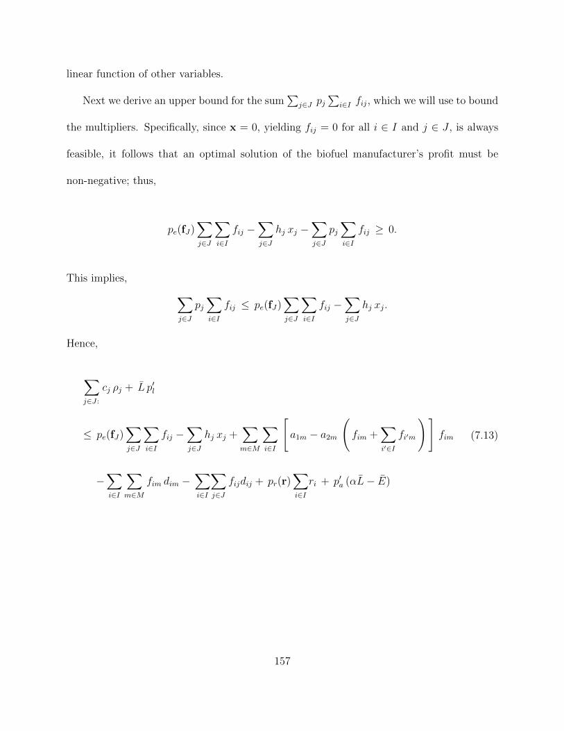
linear function of other variables.
Next we derive an upper bound for the sum∑
j∈J pj∑
i∈I fij, which we will use to bound
the multipliers. Specifically, since x = 0, yielding fij = 0 for all i ∈ I and j ∈ J , is always
feasible, it follows that an optimal solution of the biofuel manufacturer’s profit must be
non-negative; thus,
pe(fJ)∑j∈J
∑i∈I
fij −∑j∈J
hj xj −∑j∈J
pj∑i∈I
fij ≥ 0.
This implies, ∑j∈J
pj∑i∈I
fij ≤ pe(fJ)∑j∈J
∑i∈I
fij −∑j∈J
hj xj.
Hence,
∑j∈J :
cj ρj + L p′l
≤ pe(fJ)∑j∈J
∑i∈I
fij −∑j∈J
hj xj +∑m∈M
∑i∈I
[a1m − a2m
(fim +
∑i′∈I
fi′m
)]fim
−∑i∈I
∑m∈M
fim dim −∑i∈I
∑j∈J
fijdij + pr(r)∑i∈I
ri + p′a (αL− E)
(7.13)
157

Also, from (7.11c), we have p′a ≤ 1α
(p′l − pr(r)), therefore, we derive
∑j∈J :
cj ρj +E
αp′l
≤ pe(fJ)∑j∈J
∑i∈I
fij −∑j∈J
hj xj +∑m∈M
∑i∈I
[a1m − a2m
(fim +
∑i′∈I
fi′m
)]fim
−∑i∈I
∑m∈M
fim dim −∑i∈I
∑j∈J
fijdij + pr(r)∑i∈I
ri −1
αpr(r) (αL− E)
≤ ∆ , maximumx∈0,1, f ≥ 0, r≥ 0
pe(fJ)
∑j∈J
∑i∈I
fij −∑j∈J
hj xj −∑i∈I
∑m∈M
fim dim + pr(r)∑i∈I
ri
+∑m∈M
∑i∈I
[a1m − a2m
(fim +
∑i′∈I
fi′m
)]fim
−∑i∈I
∑j∈J
fijdij −1
αpr(r) (αL− E)
subject to (7.2b).
(7.14)
Therefore, we derive
ρj ≤∆
minj∈J(cj), ρj, ∀j ∈ J
pl ≤ minα∆
E,D−1(0) , pl,
pa ≤1
α(pl − pr(r)) ≤, pa.
(7.15)
158

Hence, for each j ∈ J with , we obtain the following bound 2 for pj:
pj ≤ ρj + 1αpl + min
i∈I(dij)−
1− αα
pr(r)
≤ ∆
minj∈J(cj)+ minα∆
E,D−1(0) + min
i∈I(dij) −
1− αα
pr(r) , pj.
(7.16)
Thus to upper bound the multipliers and prices, it suffices to solve a mixed concave quadratic
maximization integer program to obtain the scalar ∆ (assuming that pe(fJ) is a linear func-
tion of the total sales∑
j∈J∑
i∈I fij with nonpositive slope); from ∆ the desired bounds for
λ, ρj, pa and pj can be obtained readily. The resulting bound could presumably be tightened
by refining the above derivations.
Formulation as a mixed integer program. We also bound the sum fim +∑i′∈I
fi′m from
the above:
fim +∑i′∈I
fi′m ≤ max
(a1m − dim + αpa
a2m
, L
), f sum
im (7.17)
and
dim−a1m+a2m
(fim +
∑i′∈I
fi′m
)−αpa+pl ≤
(dim − a1m + a2m f
sumim + pl
), γim (7.18)
Moreover, for all j ∈ J with , we have
pl + ρj ≤∆
min(Eα, cj
) , ξj (7.19)
2This bound can also be used for pj corresponding to xj = 0 because such a pj has no effect on the innerand outer objective functions.
159

and
dij − pj + ρj + (1− α)pa + pl ≤[dij + ξj + (1− α)pa + pl
], γij (7.20)
Using (7.12), (7.15), (7.17), and (7.19), we obtain a mixed integer programming formu-
160

lation of the Stackelberg-Nash game (7.6):
maximizex,pJ , f , r, pa, pl
pe(fJ)∑j∈J
∑i∈I
fij −∑i∈I
∑m∈M
[dim + a2m
(fim +
∑i′∈I
fi′m
)− a1m
]fim −
∑j∈J
hjxj
−∑i∈I
∑j∈J
fijdij −∑j∈J
cjρj + pa(αL− E)− Lpl + pr(r)∑i∈I
ri (7.21a)
subject to xj, yj ∈ 0, 1 , ∀ j ∈ J (7.21b)
ui ∈ 0, 1 , ∀ i ∈ I (7.21c)
s, v, w ∈ 0, 1 , (7.21d)
zij, zim ∈ 0, 1 , ∀ i ∈ I, j ∈ J, m ∈ M (7.21e)
and for all i ∈ I, all m ∈ M , and all j ∈ J :
0 ≤ pj ≤ pjxj (7.21f)
0 ≤ fim ≤ L zim (7.21g)
0 ≤ dim − a1m + a2m
(fim +
∑i′∈I
fi′m
)− αpa + pl ≤ γim (1− zim) (7.21h)
0 ≤ fij ≤ cj zij (7.21i)
0 ≤ dij − pj + ρj + (1− α)pa + pl ≤ γij(1− zij) (7.21j)
0 ≤ ri ≤ L ui (7.21k)
0 ≤ pl − pr(r)− αpa ≤ (pl − pr(r)) (1− ui) (7.21l)
0 ≤ ρj ≤ ρj yj (7.21m)
0 ≤ cj xj −∑i∈I
fij ≤ cj ( 1− yj ) (7.21n)
dl =∑i∈I
( ∑k∈M∪J
fik + ri
)(7.21o)
0 ≤ pl ≤ pl s (7.21p)
0 ≤ L− dl ≤ L ( 1− s ) (7.21q)
0 ≤ dl ≤ L w (7.21r)
0 ≤ pl −D−1(dl) ≤ pl ( 1− w ) (7.21s)
0 ≤ pa ≤ pa v (7.21t)
0 ≤
(E −
∑i∈I
∑j∈J
fij
)≤ E (1− v) (7.21u)
and for all j ∈ J,
xj + yj ≥ 1xj ≥ zij, ∀ i ∈ I.
(7.21v)
161

The upshot of the above derivation is that the original bi-level DC-MPEC formulationof
the Stackelberg-Nash game is transformed into an equivalent mixed concave quadratic max-
imization integer programming problem (7.21); the latter can be directly solved by existing
MIQP solvers (e.g., CPLEX) or customized algorithms. Next, we will focus on developing
LR and LP based decomposition schemes to efficiently solve (7.21).
7.2.2 LR and LP based Adaptive Algorithms
In this section, we develop an adaptive relaxation algorithm that decomposes the big
MIQP model in (7.21) so as to solve it more efficiently compared to directly using commercial
solvers. We adopted two ways of relaxation techniques, LP relaxation and LR, in the same
iterative algorithm framework. Compared with LR, LP relaxation is more straightforward,
therefore, we will mainly focus on introducing our algorithm framework with LR.
7.2.2.1 Relaxed Problem
First, we introduce the LR procedure we used to decompose the problem (7.21) in an iterative
framework. Note that constraints (7.22a) and (7.22b) involve a large number of binary
variables especially when the problem is large, and this makes the MIQP (7.21) challenging
to solve for large scale problems. So we choose to relax (7.22a) and (7.22b) and add them
to the objective function as a penalty term with Lagrangian dual variables π1 = π1ij ≥ 0,
162

π2 = π2ij ≥ 0, π3 = π3
im ≥ 0, π4 = π4im ≥ 0.
fij ≤ cj zij, ∀j ∈ J, i ∈ I (7.22a)
dij − pj + ρj + (1− α)p′a + p′l + λ ≤ γij ( 1− zij ) ∀j ∈ J, i ∈ I (7.22b)
fim ≤ L zim, ∀m ∈M, i ∈ I (7.22c)
dim − a1m + a2m
(fim +
∑i′∈I
fi′m
)− αp′a + p′l ≤ γim ( 1− zim ) , ∀m ∈M, i ∈ I.
(7.22d)
where we denote γij , dij − pj + ρj + (1 − α)p′a + p′l and γim , dim − a1m + a2m ( fim +∑i′∈I fi′m )− αp′a + p′l. In addition, let V denote the solution space of the relaxed problem
(7.23) and q(π) represent the optimal objective value of the objective function of the relaxed
problem as a function of π, i.e.,
q(π) = maximizex,pJ , f , r, pa, pl ∈V
pe(fJ)∑j∈J
∑i∈I
fij −∑j∈J
hjxj −∑i∈I
[∑m∈M
fimdim +∑j∈J
fijdij
]−∑j∈J
cjρj − Lpl + pr(r)∑i∈I
ri
−∑m∈M
∑i∈I
[a2m
(fim +
∑i′∈I
fi′m
)− a1m
]fim + pa(αL− E)−
∑i∈I
∑j∈J
π1ij(fij − cjzij)
−∑i∈I
∑j∈J
π2ij(γij − γij(1− zij))−
∑i∈I
∑m∈M
π3ij(fim − Lzim)−
∑i∈I
∑m∈M
π4ij(γim − γij(1− zim))
(7.23)
The above relaxed problem can be decomposed into two subproblems:
163

(Sub-problem 1)
maximizez
∑i∈I
∑j∈J
(π1ijcj − π2
ij γij) zij +∑i∈I
∑m∈M
(π3ijL− π4
ij γim) zim
subject to (7.21e)
(7.24)
(Sub-problem 2)
maximizex,pJ , f , r, pa, pl
pe(fJ)∑j∈J
∑i∈I
fij −∑j∈J
hjxj −∑i∈I
[∑m∈M
fimdim +∑j∈J
fijdij
]−∑j∈J
cjρj
−∑m∈M
∑i∈I
[a2m
(fim +
∑i′∈I
fi′m
)− a1m
]fim + pa(αL− E)− Lpl + pr(r)
∑i∈I
ri
−∑i∈I
∑j∈J
(π1ij fij + π2
ij γij − π2ij γij)
−∑i∈I
∑m∈M
(π3im fim + π4
im γim − π4im γim)
subject to (7.21b)− (7.21d), (7.21f), (7.21k)− (7.21u)(7.25)
Under given π, subproblem 1 in (7.24) can be solved by simple inspection, while sub-
problem 2 in (7.25) is MIQP involving much fewer number of binary variables compared to
(7.21) (about |I|×(|J |+|M |)|I|×(|J |+|M |)+2|J |+|I| less). As such, the relaxed problem (7.23) can be solved
separately.
The LP relaxation of problem (7.21) is much more straightforward, i.e., we simply relax
the binary variables zim, zij related to constraints (7.22) to be continuous over [0, 1], so that
the LP relaxed problem also provides an upper bound for (7.21). The optimal solution to
the LR (or LP relaxed) problems (x∗,p∗J , f∗, r∗, p′∗l , p′∗a ) may violate the relaxed constraints.
164

However, they could be used to help obtain feasible solutions to problem (7.21), which
provides a lower bound (LB) to the true optimal objective value. We will discuss more
details regarding this procedure in the following subsection.
7.2.2.2 Computing Feasible Solutions
A key step of the relaxation algorithm in subsection 7.2.2.1 is to obtain good feasible solutions
to the original problem. We adopted the following procedure to construct a feasible solution
based on an optimal solution (x∗, p∗J) to the LR or LP relaxed problem.
If we fix the values of the variables x, pJ to be (x∗, p∗J), now to get a feasible solution for
the rest of variables, we are facing the following single level mixed complementarity problem
(MCP). By solving (7.26), we can make sure all constraints are satisfied, and thus obtain a
feasible solution.
0 ≤ fij ⊥ dij − p∗j + ρj + (1− α)p′a + p′l ≥ 0, j ∈ J
0 ≤ ρj ⊥ cj x∗j −
∑i∈I
fij ≥ 0, j ∈ J
and (7.11a), (7.11c), (7.11e)− (7.11h)
(7.26)
7.2.2.3 Adaptive Relaxation Algorithm Framework
We mainly focus on introducing our algorithmic framework based on LR, since the LP
relaxation subroutine can adapted to this algorithm in a similar manner.
To find the optimal values of the Lagrangian multipliers which leads to primal optimum,
165

we update them over iterations. The Lagrangian dual of problem (7.21) is
q∗ = minπ≥ 0
q(π).
Standard procedure of LR algorithm can be used to iteratively search for the optimal value
of dual variables π and solve the original problem. For any π, q(π) is an upper bound (UB)
to the original optimum of (7.21). The conventional sub-gradient method can be applied
to update π over iterations (Fisher, 1981). For example, in iteration n, π1 and π2 can be
updated by:
π1ij,n+1 = max
0, π1
ij,n + tn(fij − cjzij), ∀j ∈ J, i ∈ I,
π2ij,n+1 = max
0, π2
ij,n + tn(γij − γij(1− zij)), ∀j ∈ J, i ∈ I.
where tn denotes the step size in nth iteration. There are multiple ways to update the step
size (Bazaraa and Sherali, 1981; Li and Ouyang, 2011). However, one popular choice is to
update tn+1 as follows:
tn+1 =
ξn(q(πn)−LB)∑i∈I
(∑j∈J
((fij − cjzij)2 + (γij − γij(1− zij))2)+
∑m∈M
((fim − Lzim
)2+ (γim − γim(1− zim))2
)) .
where ξn is a scalar control parameter. Practical experience of LR algorithm has suggested
that it is suitable to use ξn = 2 as an initial value and gradually decrease it by a small amount
166

if q(πn) does not improve after a specified number of iterations. The algorithm terminates
when certain stopping criteria are satisfied (e.g., the maximum number of iterations is reached
or the duality gap is smaller than a tolerance).
Now we are ready to present the complete algorithm framework for solving problem and
resultantly the original DC-MPEC problem. Let F denote the complete constraint set of the
relaxed problem in (7.23), and R denote the set of the constraints (7.22), so F ∪R represent
the feasible region of the original problem (7.21). The complete algorithm framework to
solve problem (7.21) is as follows.
Step 1. Initialize the constraint set Θ0 = ∅ ∪ F , upperbound and lowerbound, andLagrangian multiplier π0.
Step 2. In iteration n, construct the relaxed problem with constraints in set Θn, andsolve the subproblems. Update the best upperbound (UB) if the current solutionprovides the tightest bound.
Step 3. Compute feasible solutions (lowerbounds) based on the solution of the relaxedproblem in step 2. Update the best lowerbound (LB) if the current solutionprovides the best objective value.
Step 4. Compute the optimality gap between UB and LB, i.e., (UB-LB)/UB. If thegap is below a user defined tolerance, terminate.
Step 5. For LR procedure, update Lagrangian multiplier πn+1 using subgradientmethod.
Step 6. Inspect the solution of the relaxed problem in step 2 by comparing the vio-lations in the current set of relaxed constraints rn ⊂ R. Choose 10 constraints(denote as v) with the highest violation in rn and add them back to the constraintset, i.e., rn+1 = rn\v. Hence the whole constraint set in a new iteration becomesΘn+1 = Θn ∪ v = rn+1 ∪ F . Go to step 2.
As for the LP relaxation based algorithm, a similar procedure applies. The only difference
167

is that we relax and gradually adding back the integrality constraints for zij, zim instead of
constraints (7.22), and step 5 can be eliminated as there is no multiplier to update in each
iteration.
7.3 Numerical Example
7.3.1 Computation Performances
To test the computational performances of our LR and LP based adaptive relaxation
algorithms and compare with commercial solvers, we apply our methodology to two problems:
one is the model without land use constraints (denote as P1) 3 and the other is our extended
model in (7.6) with land use constraints (denote as P2). For the ease of comparison, we
use the same problem setting and data sets: 1) the study area is State of Illinois where a
single biofuel company is planning to build multiple ethanol plants potentially in each county
centers; 2) we consider corn as the single feedstock type provided by farmers (i.e., farmers).
Top corn production counties (based on 2008 production data) are selected to represent
individual farms and county level corn supply data is used (Kang et al., 2010; Khanna et al.,
2008); 3) The candidate bio-refinery locations are selected based on accessibility to major
interstate highways (Kang et al., 2010; Bai et al., 2011b), and a set of local grain markets
are chosen based on proximity to the farms. 4
For the purpose of comparison, we implemented several problem instances with different
scales (i.e., |I|, |J |, |M |) from (30, 30, 30) to (50, 50, 50) and different levels of bio-refinery
3P1 is similar as the model we proposed in our previous work Bai et al. (2012).4Other data resources and parameter values are stated in detail in Bai et al. (2011b).
168

plant capacity from small size 25MGY to large size 100MGY. The LR procedure is coded in
GAMS script. Commercial solver CPLEX is used to solve the LR subproblems, and solver
PATH is used to solve the MCP subproblems. All models are solved on a desktop computer
with 2.20 GHz CPU and 1.99 GB memory.
In this case study, the following values are assumed for the cap and trade parameters:
α = 30%, E = α ∗ L = 0.3L, CRP land price pr(r) = $1/unit land 5, and the inverse
demand function for land D−1(dl) = 3.0− 0.0001dl. Computation results for P1 are listed in
Table 7.1. From these results, we can see that in general our proposed LR (and LP) based
relaxation algorithm significantly outperforms the solvers to directly solving the MIQP. Our
proposed algorithms not only greatly reduce the computation time for solving the small
cases, such as (20, 15, 10) and (20, 20, 20), but also solve those difficult problems which
CPLEX fails to solve. Besides, It successfully finds optimal or near optimal solutions to
the large cases above (30, 30, 30). As the problem scale increases, the adaptive relaxation
algorithms are more computationally beneficial. Furthermore, by comparing LR and LP
subroutines, we can see that the former shows superiority in terms of optimality gap for
larger problems, such as the (50, 50, 50) case. The rationality is that the LP based relaxation
algorithm is relatively a little naive since it gradually narrows the feasible region by simply
adding back constraints; whereas the LR procedure provides a smart way of approaching to
dual optimality by updating the multipliers, so that the computation efforts from previous
iterations can be utilized. Similar patterns in computational results are shown for P2 in
5To unify all variables and parameters, the land unit we used is the land equivalence for producing onebushel of corn
169

Table 7.2.
Table 7.1: Comparison of different solution methods on P1.
Table 7.2: Comparison of different solution methods on P2.
Meanwhile, we can also see that as the problem size increases, more computation effort
is needed and the duality gaps increases. From our computation experience, although the
relaxed problem by LR or LP is much easier to solve compared to the original MIQP, we
170

learned that solving the relaxed problem (such as the subproblem 2 in LR) still requires the
majority of computational effort. Furthermore, different capacity levels also affect the level
of difficulty, e.g., the 25MGY cases are relatively easier to solve compared with the 50 or
100 MGY cases.
7.3.2 Land Use Implications
Besides the computational observations on solution algorithms, our model also provides
implications on the optimal design of biofuel supply chain, farmland allocation patterns and
the effect of land use regulation scheme. Table 7.3 is a comparison of the optimal solutions
between P1 and P2, i.e., with and without the land use policy on the case (30, 30, 30).
Table 7.3: Comparison of itemized costs of P1 and P2 on the (30, 30, 30) case.
Under the current parameter values, the CRP land for all farmers is zero in these cases.
This is because a low CRP price is used in the model. However, we found that if plugged in
with a high enough value for pr(r), the model would result in part of the total land chosen
as CRP land. Note that all of the land is used for either biomass or food crop in the three
171

cases, so the total land demand and land price are also the same.
As expected, with the land use regulation mechanism, the optimal number of refineries
decreases and the total land use for producing biomass is reduced accordingly in all three
cases. The percentage of land use for biomass is exactly equal to the regulated cap, i.e.,
E/L. Therefore, we have a non zero price pa for the land use allowance. It means that
growing biomass and producing ethanol are in general profitable for most farms and the
biofuel manufacturer, so that farmer’s willingness to pay for the allowance is positive, and
the manufacturer’s willingness to pay for biomass is high enough to procure up to the amount
corresponding the land use limit. The price for biomass procurement in P2 is actually higher
than that in P1, the reason is that now the competition between land use is in favor of food
market, because farmers can get extra credits by selling the permits instead of consuming
them. As a result, this allowance price pa is partially added on to the biomass procurement
price.
Furthermore, it can be seen that although the biofuel manufacturer’s profit shrinks by
a small portion, the profit for the whole supply chain actually increases. Under the current
model setting, we can conclude that the government regulation helps improve the overall
economic benefit of the whole supply chain. However, this conclusion may not be accurate
since we did not consider the impact on fuel markets and substitute goods such as gasoline.
7.4 Conclusion
We have proposed a possible land use regulation scenario and integrate it into the com-
172

petitive biofuel supply chain design problem that addresses the interactions among biofuel
industry expansion, farmers land use, and food, fuel, farmland markets. We presented a
base Stackelberg-Nash game model with land use constraints, and further a cap and trade
mechanism that implements the land use constraints. We further developed two solution
algorithms to solve the DC-MPEC models, i.e., LR and LP based adaptive relaxation algo-
rithms, and showed their effectiveness and efficiencies in solving different sizes of problems.
In addition, insights are drawn from a comprehensive numerical study in the context of Illi-
nois. Under the land use constraint, less farmland is used to produce energy crops, and as a
result fewer refineries are built. The proposed cap and trade system results in less profit for
the biofuel manufacturer, but more profit for the entire food and fuel supply chain.
Future work should address more detailed problems in the cap and trade system, such as
how policy makers could determine the optimal land use cap E which we assume a constant
in this chapter, and what would be a good allowance allocation policy by comparing different
allocation rules. It is also of interest to explore possible contract scenarios between farmers
and biofuel manufacturers under governmental regulations, and their effects on risk reduction
and the biofuel supply chain design.
173

Chapter 8
Conclusions and Future ResearchOpportunities
8.1 Conclusions
In this work, we have developed several mathematical models to address the biofuel sup-
ply chain system design. We have incorporated or accounted for various factors such as
feedstock price dynamics, and operation disruption risks, as well as economic and social
impacts including impacts on the traffic network, food market and land use. The biofuel
supply chain is such a complex system of subsystems (e.g., transportation, refinery opera-
tion, farmland, water supply, etc), that it is extremely challenging to build a system model
encompassing details of all the subsystems together. We followed the approach to start from
a simple classic model and build upon it to incorporate more factors or extend to broader
horizons step by step.
We first assessed the impact of biomass and ethanol traffic and introduced it into the tra-
ditional facility location design model to decide the optimal location of refineries and biomass
and ethanol transportation flow patterns that minimize the total system cost. An MINLP
174

optimization model is proposed to address the bio-refinery location problem and biomass and
ethanol traffic assignment problem in an integrated framework. The methodology proposed
in this study is actually quite general; it can also be used to improve other transportation
planning and supply chain design (e.g., traffic impact studies for city planning) wherever
a strong bidirectional relationship exists between road congestion pattern and new facility
location choices. An LR based heuristic algorithm is proposed to solve the model, and two
B&B algorithms (with LR or LP relaxation bounding procedures) are introduced to further
improve the solution to optimality. Several hypothetical example problems are used to ex-
amine the effectiveness of the three algorithms. The LR heuristic algorithm is shown to find
good feasible solutions within a relatively short time. It often leaves a small optimality gap
which can be closed by the B&B algorithms for small or moderate size problems. For larger
scale networks, the B&B algorithm with LP or LR can still be used to reduce the optimality
gap. In the Illinois case study, we compare the model results with a benchmark solution (i.e.,
not considering congestion), and the congestion-related costs caused by biomass shipment
flow are estimated. The proposed solution considerably reduced the transportation costs of
biomass shipments, compared with the benchmark result. It is also shown that the conges-
tion experienced by the public can be reduced by the proposed model. Finally, we presents
a series of sensitivity analyses to reveal how the values of social-economic parameters affect
the optimal design.
Then, we extended the model to address a joint optimization problem of biofuel supply
chain design and pavement rehabilitation activities. The integrated model addresses the
175

impact of biofuel supply chain expansion on the supporting transportation infrastructures
and minimizes the total costs related to the biofuel supply chain (refinery construction and
materials/products transportation cost), the existing roadway users (public travel delay) and
the pavement infrastructures (agency cost and vehicle operating cost). A bi-level MINLP
was proposed to simultaneously determine the production refinery location, biomass and
ethanol shipment flow, and pavement rehabilitation plan. To solve this challenging problem,
a LR based algorithm was used to decompose the original model into sub-problems, and an
iterative penalty method is developed to solve the bi-level nonlinear sub-problem. A numer-
ical study on a hypothetical transportation network was conducted. Computational results
showed that the proposed algorithm was able to solve the problem effectively. Managerial
insights were also drawn to show the effect of the joint optimization compared with the
benchmark model ignoring the impacts on pavement.
We further studied two stochastic biofuel supply chain design problem as an extension
of the deterministic supply chain design model that we have developed. We first addressed
a stochastic biofuel supply chain design problem under feedstock supply and final product
demand uncertainties by Monte Carlo method. A scenario based stochastic program is
proposed and an LR based solution algorithm is developed for this specific problem. Stratified
sampling and antithetic sampling methods are implemented to generate possible supply and
demand scenarios based on certain probabilistic distributions. This methodology is applied
to the Sioux Falls network example and a series of numerical results are obtained. We solved
the problem under different number of samples of supply and demand scenarios. It is found
176
that the solution (such as optimal number of refineries and total cost) follows a trend to
converge to a steady value. It is found that the more scenarios are generated and plugged
into the problem, the more accurate solution will be obtained. In addition, we performed a
sensitivity analysis of the optimal solution to problem M2 with respect to the fixed refinery
investment cost. Considering 50 scenarios, the model produced consistent results of the
optimal number of selected refineries and the total costs as the fixed refinery building cost
increases.
Furthermore, we addressed a reliable supply chain design problem through a case study
of the ongoing biorefinery infrastructure planning in the State of Illinois. Reliable facility
location design models are applied to determine optimal refinery locations that can hedge
against the risk of refinery operation disruptions and the consequence of enormous social
disbenefits. Both a discrete and a continuous version of the reliable location models have
been implemented. The data sets used in this case study are extracted from the Illinois
biomass supply databases and various technical reports on refinery disruptions. From the
case study, we found that the reliable location models can efficiently solve the supply chain
design problem while each offers certain unique advantages. For example, the discrete model
solution achieves better optimality while the continuum model has superior computational
tractability. From our numerical results, we find that the optimal refinery locations tend
to be at places with high biomass supply and low disruption probability. The sensitivity
analysis further reveals how refinery disruption probabilities and penalty cost from service
loss affect optimal location design and total expected system cost.
177

Another key issue related to biofuel supply chain development is the interactions among
biofuel supply chain design, agricultural land use and local food market, so we switched focus
to the economic behaviors of the stakeholders in the biofuel supply chain, and incorporate
them into the supply chain design model. We mainly developed a bi-level noncooperative
game model (the Stackelberg leader-follower game) in the form of DC-MPEC: the upper
level problem determines the optimal biofuel refinery locations and feedstock procurement
prices that maximize a biofuel company’s profit; and the lower level problems are individual
farmers’ land use optimization problem. The solution approach that transforms the prob-
lem into an MIQP based on KKT conditions is developed under the assumption of linear
demand function. We further proposed a cooperative game model. It is found that the
advent of a new biofuel supply chain will alter the equilibrium of corn demand/supply and
spatial corn price pattern. Under the optimal supply chain design scheme, building refiner-
ies will have significantly different effects on the average corn market price under different
industry scenarios (cooperative vs. noncooperative). Besides, the existence of biorefineries
provides new land use choices for farms in the proximity. Farmers who use to sell corn to
local food markets will ship part of the corn to nearby refineries where more profits could
be earned. Finally, compared with the noncooperative game scenario, the system-optimal
objective for biofuel supply chain design under the cooperative game scenario is shown to
save transportation cost and to generate higher profit for the whole supply chain.
We then build on our previous work to develop a competitive supply chain design model to
account for the possible governmental regulations/policies on agricultural land use and GHG
178

emission for the emerging biofuel industry. A land use permit cap-and-trade mechanism and
a life cycle GHG emission constraint are adopted to model the government’s incentives to
limit the land usage for biomass crops and emission associated with biofuel production. We
develop two iterative solution algorithms based on LR and LP to transform, decompose, and
solve such highly challenging problems. An equivalent DC-MPEC formulation is introduced
to facilitate reformulating it into an MIQP, and LR and LP relaxation methods are applied
to decompose the original DC-MPEC into easier subproblems. Finally, an effective way of
obtaining feasible solutions to the original DC-MPEC problem is introduced to help search
for the optimal solution and provide lowerbounds of the optimal objective value. A set of
numerical experiments illustrates computational performance of the proposed methodoloty.
In most tested cases, the iterative relaxation algorithm based on LR or LP is able to find
optimal (for small scale problems) or near-optimum solutions (for moderate or large scale
problems) within a reasonable amount of time. Compared with our previous MIQP reformu-
lation method, the iterative approach shows superior performances for larger scale problems,
which is able to find good feasible solutions for the cases which were originally unsolvable
by many other methods. Insights are also drawn from the numerical results.
In summary, our proposed methodology can be implemented to find optimal design so-
lutions of other emerging chain in a competitive market environment in many contexts and
other network design problems with equilibrium constraints. Our solution algorithms for
MIP, MINLP and DC-MPEC also provide useful practices for solving similar types of math-
ematical programs.
179

8.2 Future Research Opportunities
Overall, we can see many future research opportunities in biofuel supply chain design
problems. Methodologically, the limitation of the LR based method mainly lies in the non-
negligible duality gap for some large cases, so further research efforts shall be devoted to
improve the quality of both upper and lower bounds. In the modeling side, our modeling
framework can be used as a helpful analytical tool to evaluate the potential impacts on
different policies scenarios for land use, emission or other environmental regulations. For
example, the biofuel is believed to save GHG emission compared to fossil fuel, so production
credit or tax reduction may be given by government in favor of biofuel. It is interesting
to look into how these possible leverages would affect the optimal design of a economically
and socially sustainable biofuel supply chain. Noting the variance of social welfare across
different business scenarios, it is particularly of interest to design effective mechanisms that
will provide the non-cooperative parties with incentives to cooperate, thereby enabling the
overall system to achieve a higher overall welfare. Future study could also consider more
sophisticated land competition among different kinds of conventional food corps and energy
crops such as cellulosic biomass. Besides, to maximize net social benefit, the impact of
biofuel supply chain design on food and fuel consumer surpluses could be considered in the
objective of biofuel supply design problem.
In addition, we have dealt with uncertainties on supply/demand and production dis-
ruption in this work, however, there are many more complex unpredictable factors such as
weather and economy that affect a biofuel supply chain from its upstream suppliers to down
180

stream customers, as well as other supporting subsystems such as water supply and trans-
portation infrastructure. It would be interesting to look into the cascading effects of the
unexpected changes in one subsystem to all others in the biofuel production and distribution
processes and how to design a system to be robust and resilient against all possible adverse
conditions.
Although this dissertation work addressed biofuel supply chain design with the impacts
of several subsystems, such as the transportation, agricultural land use and food market
equilibrium, there are other important infrastructure subsystems or factors that play roles
in the long run sustainability of the biofuel industry, such as water supply for both irrigation
and ethanol production, biomass crop production and collection, fuel market of different
substitute goods, and uncertainties from natural and social environments. None of the
proposed models includes all details of every subsystems. It is an extremely challenging
problem to model the comprehensive system of subsystems with different decision making
integrated simultaneously, but such model will be valuable to provide clearer visions for
policy makers, manufacturers and suppliers on the prosperity of this new industry to meet
the national demand.
181

References
Abdulaal, M., LeBlanc, L., 1979. Continuous equilibrium network design models. Trans-
portation Research Part B: Methodological 13 (1), 19–32.
Aboolian, R., Berman, O., Krass, D., 2008. Optimizing pricing and location decisions for
competitive service facilities charging uniform price. Journal of the Operational Research
Society 59 (11), 1506–1519.
Ahmedov, Z., Power, G. J., Vedenov, D., Fuller, S., Mccarl, B., Vadali, S., July 2009. A
spatial equilibrium model of the impact of bio-fuels energy policy on grain transportation
flows. In: Proceedings of Agricultural & Applied Economics Association 2009 Annual
Meeting. Milwaukee, Wisconsin.
Anderson, J., Coble, K., 2010. Impact of renewable fuels standard ethanol mandates on the
corn market. Agribusiness 26 (1), 49–63.
Bai, L., Mitchell, J., Pang, J., 2011a. On Convex Quadratic Programs with Complementarity
Constraints. Manuscript. Rensselaer Polytechnic Institute.
182

Bai, Y., Hwang, T., Kang, S., Ouyang, Y., 2011b. Biofuel refinery location and supply chain
planning under traffic congestion. Transportation Research Part B 45 (1), 162–175.
Bai, Y., Ouyang, Y., Pang, J., 2012. Biofuel supply chain design under competitive agricul-
tural land use and feedstock market equilibrium. Energy Economics, In Press.
Ban, X., Liu, H., Lu, J., Ferris, M., 2006. Decomposition scheme for continuous network
design problem with asymmetric user equilibria. Transportation Research Record: Journal
of the Transportation Research Board 1964 (1), 185–192.
Bazaraa, M., Sherali, H., 1981. On the choice of step size in subgradient optimization.
European Journal of Operational Research 7 (4), 380–388.
Benjamin, C., Houee-Bigot, M., July 29-August 1 2007. Measuring competition between
non food and food demand on world grain markets: Is biofuel production compatible with
pressure for food production? Selected Paper Prepared for Presentation at the American
Agricultural Economics Association Annual Meeting.
Berkes, F., Colding, J., Folke, C. E., 2003. Navigating Social-Ecological Systems: Building
Resilience for Complexity and Change. Cambridge University Press, Cambridge, UK.
Berkes, F., Seixas, C., 2005. Building resilience in lagoon social-ecological systems: a local-
level perspective. Ecosystems 8, 967–974.
Brown, R., Orwig, E., Nemeth, J., Rocha, C., 2007. The economic potential for ethanol
expansion in illinois.
183

Chen, X., Huang, H., Khanna, M., Onal, H., April 2010. Meeting the mandate for biofuels:
Implications for land use, greenhouse gas emissions and social welfare. In: Proceedings of
the Nber Meeting on Agricultural Economics and Biofuels.
Chen, Y., Liu, A., Hobbs, B., 2011. Economic and emissions implications of load-based,
source-based, and first-seller emissions trading programs under california ab32. Operations
Research 59 (3), 696–712.
Daskin, M., 1995. Network and Discrete Location: Models, Algorithms, and Applications.
John Wiley, New York.
Dicks, M., Campiche, J., Ugarte, D., Hellwinckel, C., Bryant, H., Richardson, J., 2009.
Land use implications of expanding biofuel demand. Journal of Agricultural and Applied
Economics 41 (2), 435–453.
Ellinger, P., 2008. Ethanol plant simulator. department of agricultural and consumer eco-
nomics, university of illinois at urbana-champaign, urbana, il.
EPA, U., 2007. Renewable fuel standard implementation.
URL http://www.epa.gov/otaq/renewablefuels/index.htm.
Ervola, A., Lankoski, J., 2011. Agriculture and climate change: Socially optimal production
and land use. In: Proceedings Ofeuropean Association of Environmental and Resource
Economists 18th Annual Conference. Rome.
Facchinei, F., Pang, J., 2003. Finite-Dimensional Variational Inequalities and Complemen-
tarity Problems, Volumes I and Ii. Springer-Verlag, New York.
184

Feng, H., Babcock, B., 2008. Impacts of Ethanol on Planted Acreage in Market Equilibrium.
Center for Agricultural and Rural Development, Iowa State University, Ames, Ia, Usa,
http://www.card.iastate.edu/publications/synopsis.aspx?id=1081.
Fisher, M., 1981. The lagrangian relaxation method for solving integer programming prob-
lems. Management Science 27 (1), 1–18.
Friesz, T., Tobin, R., Miller, T., 1989. Existence theory for spatially competitive network
facility location models. Annals of Operations Research 18 (1), 267–276.
Fukushima, M., 2011. Restricted generalized nash equilibria and controlled penalty algo-
rithm. Computational Management Science 8 (3), 201–218.
Gabriel, S., Leuthold, F., 2010. Solving discretely-constrained mpec problems with applica-
tions in electric power markets. Energy Economics 32, 3–14.
Gabriel, S., Shim, Y., Conejo, A., De La Torre, S., Garcia-Bertran, R., 2010. A benders
decomposition method for discretely constrained mathematical programs with equilibrium
constraints. Journal of the Operational Research Society 61, 1404–1419.
Gallagher, P., Shapouri, H., Price, J., Schamel, G., Brubaker, H., 2003. Some long-run effects
of growing markets and renewable fuel standards on additives markets and the us ethanol
industry. Journal of Policy Modeling 25 (6-7), 585–608.
Garcia-Bertrand, R., Conejo, A., Gabriel, S., 2006. Electricity market near-equilibrium under
locational marginal pricing and minimum profit conditions. European Journal of Opera-
tions Research 174, 457–479.
185

Gehlhar, M., Somwaru, A., Dixon, P., Rimmer, M., Winston, R., 2010. Economywide impli-
cations from us bioenergy expansion. American Economic Review: Papers and Proceedings
100 (2), 172–177.
Geoffrion, A., Graves, G., 1974. Multicommodity distribution system design by benders
decomposition. Management Science 20 (5), 822–844.
Hanjoul, P., Hansen, P., Peeters, D., Thisse, J., 1990. Uncapacitated plant location under
alternative spatial price policies. Management Science 36 (1), 41–57.
HCM, 2000. Highway Capacity Manual (HCM). Transportation Research Board.
Hobbs, B., Metzler, C., Pang, J., 2000. Strategic gaming analysis for electric power networks:
An mpec approach. IEEE Transactions on Power Systems 15, 638–645.
Hu, J., Mitchell, J., Pang, J., Bennett, K., Kunapuli, G., 2008. On the global solution of
linear programs with linear complementarity constraints. Siam Journal on Optimization
19, 445–471.
Hu, J., Mitchell, J., Pang, J., Yu, B., 2011a. On linear programs with linear complementarity
constraints. Journal on Global Optimization, 1–23.
Hu, J., Mitchell, J., Pang, J., Yu, B., 2011b. On linear programs with linear complementarity
constraints. Journal on Global Optimization, 1–23.
IAPC, 2012. Usda agricultural projections to 2021. Tech. rep.
186

Johansson, D., Azar, C., 2007. A scenario based analysis of land competition between food
and bioenergy production in the u.s. Climatic Change 82 (3), 267–291.
Johnson, D., Lenstra, J., Kan, A., 1978. The complexity of the network design problem.
Networks 8 (4), 279–285.
Kang, S., Onal, H., Ouyang, Y., Scheffran, J., Tursun, D., 2010. Optimizing the biofuels
infrastructure: Transportation networks and biorefinery locations in illinois. In: Khanna,
M., Scheffran, J., Zilberman, D., Dinar, A., Zilberman, D. (Eds.), Handbook of Bioenergy
Economics and Policy. Vol. 33 of Natural Resource Management and Policy. Springer New
York, pp. 151–173.
Karp, L., Mccalla, A., 1983. Dynamic games and international trade: An application to the
world corn market. American Journal of Agricultural Economics 65 (4), 641–650.
Keeney, R., Hertel, T., 2009. The indirect land use impacts of u.s. biofuel policies: the im-
portance of acreage, yield, and bilateral trade responses. American Journal of Agricultural
Economics 91 (3), 895–909.
Khanna, M., Dhungana, B., Clifton-Brown, J., 2008. Costs of producing miscanthus and
switchgrass for bioenergy in illinois. Biomass & Bioenergy 32 (6), 482–493.
Krawczyk, J., 2007. Numerical solutions to coupled-constraint (or generalised nash) equilib-
rium problems. Computational Management Science 4 (2), 183–204.
Larson, J., English, B., He, L., 2008. Economic analysis of farm-level supply of biomass feed-
187

stocks for energy production under alternative contract scenarios and risk. In: Proceedings
of Integration of Agricultural and Energy Systems Conference. Atlanta, GA.
Li, X., Ouyang, Y., 2011. Reliable sensor deployment for network traffic surveillance. Trans-
portation Research Part B 45 (1), 218–231.
Li, Y., Madanat, S., 2002. A steady-state solution for the optimal pavement resurfacing
problem. Transportation Research Part A: Policy and Practice 36 (6), 525–535.
Lu, Y., 2006. Robust transportation network design under user equilibrium. Master’s thesis.
Luo, Z., Pang, J., Ralph, D., 1996. Mathematical Programs with Equilibrium Constraints.
Cambridge University Press, Cambridge, England.
Mapemba, L., 2005. Cost to deliver lignocellulosic biomass to a biorefinery. Ph.D. thesis,
the Oklahoma State University.
URL http://bioeconomyblog.blogspot.com/2007/06/dissertation-cost-to-deliver.html.
Mcnew, K., Griffith, D., 2005. Measuring the impact of ethanol plants on local grain prices.
Review of Agricultural Economics 27 (2), 164–180.
Mcvey, M., Vaughn, M., Baumel, C., August 2007. Semis compared by farm size. Feedstuffs.
Meng, Q., Yang, H., Bell, M., 2001. An equivalent continuously differentiable model and a
locally convergent algorithm for the continuous network design problem. Transportation
Research Part B: Methodological 35 (1), 83–105.
188

Meyer, M., Miller, E., 2001. Urban Transportation Planning: a Decision-Oriented Approach,
Second Edition. New York: Mcgraw-Hill.
Miller, T., Friesz, T., Tobin, R., 1992a. Heuristic algorithms for delivered price spatially
competitive network facility location problems. Annals of Operations Research 34 (1),
177–202.
Miller, T., Tobin, R., Friesz, T., 1992b. Network facility-location models in stackelberg-nash-
cournot spatial competition. Papers in Regional Science 71 (3), 277–291.
Mitchell, J., Pang, J., Yu, B., 2011. Optimization methods and software. Submitted to
Journal on Global Optimization.
O’Brien, D., Woolverton, M., 2009. How grain ethanol plants affect local grain prices.
Oladosu, G., Kline, K., Uria-Martinez, R., Eaton, L., 2011. Sources of corn for ethanol
production in the united states: a decomposition analysis of the empirical data. Biofuels,
Bioproducts and Biorefining 5 (6), 640–653.
Ouyang, Y., 2007. Pavement resurfacing planning on highway networks: a parametric policy
iteration approach. ASCE Journal of Infrastructure Systems 13 (1), 65–71.
Ouyang, Y., Madanat, S., 2004. Optimal scheduling of rehabilitation activities for multiple
pavement facilities: exact and approximate solutions. Transportation Research Part A
38 (5), 347–365.
189

Ouyang, Y., Madanat, S., 2006. An analytical solution for the finite-horizon pavement resur-
facing planning problem. Transportation Research, Part B: Methodological 40 (9), 767–
778.
Paterson, W., 1990. Quantifying the effectiveness of pavement maintenance and rehabilita-
tion. In: Sixth REAAA Conference Proceedings. Vol. 1. Kuala Lumpur, Malaysia.
Pfuderer, S., Castillo, M., 2008. The impact of biofuels on commodity prices. department
for environment, food and rural affairs. Tech. rep.
Rajagopal, D., Sexton, S., Hochman, G., Roland-Holst, D., Zilberman, D., et al., 2009.
Model estimates food-versus-biofuel trade-off. California Agriculture 63 (4), 199–201.
RITA, 2008. National transportation atlas database 2008.
URL http://www.bts.gov.proxy2.library.illinois.edu/
Schnepf, R., 2006. Price determination in agricultural commodity markets: a primer. crs
report for congress. Tech. rep.
URL http://www.nationalaglawcenter.org/assets/crs/rl33204.pdf.
Serra, D., Revelle, C., 1999. Competitive location and pricing on networks. Geographical
Analysis 31 (2), 109–129.
Sexton, S., Zilberman, D., ???? Biofuel impacts on climate change, the environment and
food - report to the renewable fuels agency. Tech. rep., Department of Agricultural and
Resource Economics, University of California, Berkeley.
190
Sheffi, Y., 1985. Urban Transportation Networks: Equilibrium Analysis with Mathematical
Programming Methods. Prentice Hall.
Shen, W., Wynter, L., 2011. A new one-level convex optimization approach for estimating
origin-destination demand. Tech. Rep. W1104-065, IBM Research Report: Matheatics.
Tobin, R., Friesz, T., 1986. Spatial competition facility location models: Definition, formu-
lation and solution approach. Annals of Operations Research 6 (3), 47–74.
Tsunokawa, K., Schofer, J., 1994. Trend curve optimal control model for highway pavement
maintenance: case study and evaluation. Transportation Research Part A 28 (2), 151–166.
Tyner, W., Taheripour, F., 2008. Biofuels, policy options, and their implications: Analy-
ses using partial and general equilibrium approaches. Journal of Agricultural and Food
Industrial Organization 6 (2), 1–17.
USDA, 2011a. Measuring the indirect land-use change associated with increased biofuel
feedstock production: A review of modeling efforts - report to congress. Tech. rep., the
USDA Economic Research Service and Office of the Chief Economist.
USDA, F., 2011b. Conservation reserve program (crp).
URL http://www.fsa.usda.gov/
USDA-AMS, 2010. Grain prices at illinois interior country elevators.
URL http://www.ams.usda.gov/mnreports/gx gr113.txt.
Vedenov, D., Fuller, S., Power, G., Ahmedov, Z., Vadali, S., Burris, M., 2010. Bio-fuels
191

energy policy and grain transportation flows: Implications for inland waterways and short
sea shipping. Tech. rep., Research and Innovative Technology Administration, Department
of Transportation.
Walsh, M., De La Torre Ugarte, D., Shapouri, H., Slinsky, S., 2003. Bioenergy crop produc-
tion in the united states: Potential quantities, land use changes, and economic impacts on
the agricultural sector. Environmental and Resource Economics 24 (4), 313–333.
Weber, A., 1957. Theory of the Location of Industries. University of Chicago Press, IL.
Wu, T., Lin, J., 2003. Solving the competitive discretionary service facility location problem.
European Journal of Operational Research 144 (2), 366–378.
Yang, H., Bell, M., 1998. Models and algorithms for road network design: a review and some
new developments. Transport Reviews 18 (3), 257–278.
Zhao, J., Hobbs, B. F., Pang, J. S., 2010. Long-run equilibrium modeling of emissions
allowance allocation systems in electric power markets. Operations Research 58 (3), 529–
548.
Zhao, X., Luh, P., 1998. Fuzzy gradient method in lagrangian relaxation for integer program-
ming problems. In: Decision and Control, 1998. Proceedings of the 37th IEEE Conference
on. Vol. 3. IEEE, pp. 3372–3377.
192

Appendix A
Proof for Propositions
Proposition 2. In an optimal solution, if αω2 − λ ∗ γ − 2Ω1Ω2Ω3 ≥ 0, e2 − r > 0, and
g1 > 0.5, then the objective function (4.23) and constraints (4.14m) are convex.
(where α = π1e0 + π2e20, ω = π3 + π4e2, λ = π1e0 + 2π2e0e2, and γ = π4e0 + π5, Ω1 =
lc1r(m1g3 +m2)(2g1 − 1)log−1 g11−g1 , Ω2 = (e2 − r)m1g2, Ω3 = c1g1 +m1g2e0.)
Proof. According to (4.2), (4.8), and (4.9), we expand equation (4.11) which results in
the following formulation.
∆τ(b) = log(g1
1− g1
)b−1, (A.1)
where g1 ≥ 0.5. Then, based on (4.1), and (4.9) the prorated agency cost per unit length
per year will be as follows.
M(b) =l(m1w
∗(b) +m2)
∆τ(b), (A.2)
M(b) =π1(x+ z)b+ π2b
2
π3 + π4b+ π5(x+ z), (A.3)
193

where π1 = lc1g1(g3m1 + m2), π2 = lm21g2g3 + lm1m2g2, π3 = −rm1g2log( g1
1−g1 ), and π4 =
m1g2log( g11−g1 ), and π5 = g1c1log( g1
1−g1 ). Let X.= x+z denotes the total flow, and b = φ(X) =
e0X + e2 (according to (4.14b), and assuming e0 = e1 , ∀a ∈ A) define the deterioration rate
of the pavement as a function of total traffic. Therefore, the M(X) is as follows.
M(X) =π1X(e0X + e2) + π2(e0X + e2)2
π3 + π5X + π4(e0X + e2). (A.4)
Thus, the first and second order derivatives of M(X) with respect to X are as follows.
dM
dX=dM
db
db
dX=π1π3e2 + 2π2π3e0e2 + (π1e0 + π2e
20)((π4e0 + π5)X2 + 2(π3 + π4e2)X)
(π3 + π4e2 + (π4e0 + π5)X)2e0,
(A.5)
d2M
dX2=d2M
db2
db
dX+dM
db
d2b
dX2=
2π3(π2π3 − π1π4)
(π3 + π4e2 + (π4e0 + π5)X)3e0. (A.6)
Inserting back the πi, i = 1, ..., 4 values, we will have
d2M
dX2=
αω2 − λ ∗ γlog3 g1
1−g1 (m1g2e2 − rm1g2 + (c1g1 +m1g2e0)X)3, (A.7)
where α = π1e0 +π2e20, ω = π3 +π4e2, λ = π1e0 +2π2e0e2, and γ = π4e0 +π5. Now, we derive
the average cost due to pavement condition for daily users according to (4.3) as follows.
C(x, z, b) = c0t(x, z) + lc1s(t) + c2. (A.8)
194

Therefore,
C(x, z, b) = c0t(x, z) +
∫ ∆τ
0(lc1s(t) + c2)dt
∆τ, (A.9)
To derive the average user cost due to the roughness, we assume that the traffic do not vary
over time for simplicity.
∫ ∆τ
0(lc1s(t) + c2)(x+ z)dt∫ ∆τ
0(x+ z)dt
≈∫ ∆τ
0(lc1s(t) + c2)dt
∆τ= (2g1 − 1)log−1 g1
1− g1
lc1s∗ + c2. (A.10)
Then,
C(x, z, b) = c0t(x, z) + (2g1 − 1)log−1 g1
1− g1
lc1s∗ + c2, (A.11)
and, according to (4.8) the user cost under optimal rehabilitation plan as a function of
traffic and deterioration rate can be written as below.
C(x, z, b) = c0t(x, z) + lc1r(m1g3 +m2)
g1c1(x+ z) + (b− r)m1g2
(2g1 − 1)log−1 g1
1− g1
+ c2. (A.12)
Then, cr(b) will be as follows.
cr(X) =Ω1
Ω2 + Ω3X, (A.13)
where Ω1 = lc1r(m1g3 + m2)(2g1 − 1)log−1 g11−g1 , Ω2 = (e2 − r)m1g2, Ω3 = c1g1 + m1g2e0.
Thus, the first and second order derivatives of cr(b) with respect to b are as the following.
dcrdX
=−Ω1Ω3
(Ω2 + Ω3X)2, (A.14)
195
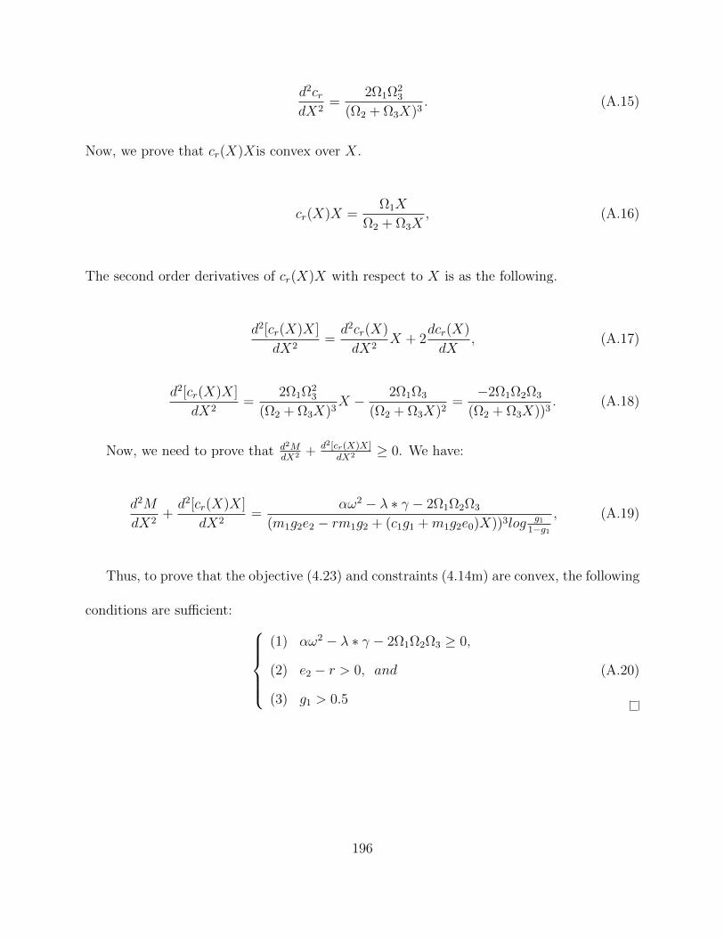
d2crdX2
=2Ω1Ω2
3
(Ω2 + Ω3X)3. (A.15)
Now, we prove that cr(X)Xis convex over X.
cr(X)X =Ω1X
Ω2 + Ω3X, (A.16)
The second order derivatives of cr(X)X with respect to X is as the following.
d2[cr(X)X]
dX2=d2cr(X)
dX2X + 2
dcr(X)
dX, (A.17)
d2[cr(X)X]
dX2=
2Ω1Ω23
(Ω2 + Ω3X)3X − 2Ω1Ω3
(Ω2 + Ω3X)2=−2Ω1Ω2Ω3
(Ω2 + Ω3X))3. (A.18)
Now, we need to prove that d2MdX2 + d2[cr(X)X]
dX2 ≥ 0. We have:
d2M
dX2+d2[cr(X)X]
dX2=
αω2 − λ ∗ γ − 2Ω1Ω2Ω3
(m1g2e2 − rm1g2 + (c1g1 +m1g2e0)X))3log g11−g1
, (A.19)
Thus, to prove that the objective (4.23) and constraints (4.14m) are convex, the following
conditions are sufficient: (1) αω2 − λ ∗ γ − 2Ω1Ω2Ω3 ≥ 0,
(2) e2 − r > 0, and
(3) g1 > 0.5
(A.20)
196